feeding of nickel-based alloys - university of...

Feeding of Nickel-Based Alloys

Kent D. Carlson, Shouzhu Ou and Christoph Beckermann

Department of Mechanical and Industrial Engineering

The University of Iowa, Iowa City, IA 52242

Abstract

Building on the successful creation of more accurate, less conservative feeding distance rules for carbon and low alloy (C&LA) and high alloy steel castings, a similar project is underway to develop feeding distance rules for the nickel-based alloys CZ-100, M-35-1 and CW-12MW, as well as for the austenitic stainless steel CN-7M. Casting trials were performed at five foundries to produce experimental feeding distance results for a total of 55 plates of varying lengths. In order to develop the property databases necessary to simulate these alloys, temperature data was recorded for each alloy during the casting trials. This measured data was then used in conjunction with material property simulation to develop the necessary property data for each alloy, including the solidification path. This property data was used to simulate the casting trials. Good agreement between the simulation results and the radiographic testing results for the castings has been obtained. Future work will include the development of general feeding and risering rules for these high-nickel alloys.

becker

Text Box

Carlson, K.D., Ou, S., and Beckermann, C., “Feeding of Nickel-Based Alloys,” in Proceedings of the 58th SFSA Technical and Operating Conference, Paper No. 3.3, Steel Founders' Society of America, Chicago, IL, 2004.

1. Introduction Feeding distance in a steel casting is defined as the distance over which a riser can provide feed metal resulting in a sound casting. This is an important concept for steel foundries, because knowledge of feeding distances allows foundries to produce sound castings with a reasonable number of risers, which helps to maximize casting yield. Due to the importance of feeding distances, a great deal of effort has been expended to develop rules to determine riser feeding distances in steel castings. In 1973, the Steel Founders’ Society of America (SFSA) published a foundry handbook entitled Risering Steel Castings[1]; this handbook provided charts, nomographs and equations for calculating feeding distances for carbon and low alloy (C&LA) and several high alloy steels. While the feeding guidelines in this handbook have been widely used in industry for the past thirty years, it is generally accepted that these rules can be overly conservative in many situations. To address the need for more accurate, less conservative feeding rules, the present authors developed a new set of C&LA feeding distance rules[2-4], followed by an analogous set of rules for high alloy steel grades CF-8M, CA-15, HH, HK and HP[5]. Both sets of rules were developed by performing plate casting trials and performing corresponding casting simulations of these trials. Through this work, a correlation was developed between the Niyama criterion (a local thermal parameter) and radiographic soundness. It was found that the same correlation was valid for both C&LA and high alloy steels. Once this correlation was established, a large number of simulations were performed in order to determine feeding distances for a wide variety of casting conditions. Based on the resulting information, a new set of feeding distance rules was designed to produce radiographically sound castings at 2 pct sensitivity. The new feeding distance rules are valid for both C&LA and high alloy steels. Rules are provided for end-effect feeding distance and lateral feeding distance for top risers, as well as feeding distance for side risers. In addition, multipliers are provided to apply these rules with end chills and drag chills, as well as to tailor these rules to different steel alloy compositions, sand mold materials and pouring superheats. These new rules are shown to provide longer feeding distances in most casting situations than previously published rules. Based on the success of these new feeding distance rules, the steel foundry industry (through the SFSA) expressed interest in the development of similar feeding distance rules for four additional alloys: three nickel-based alloys (CW-12MW, CZ-100 and Monel-35-1) and an austenitic stainless steel (CN-7M) with a large nickel component. The nominal compositions for each of these alloys are provided in Table 1. The research plan is to develop these rules in a manner similar to the C&LA and high alloy rules discussed in the previous paragraph: plate casting trials performed in conjunction with corresponding casting simulations will provide correlations between simulation variables and experimental results. Once correlations are developed, extensive simulation will be used to develop feeding distance rules for a wide range of casting conditions. One substantial difference between the current feeding distance development and the previous work by the present authors is the need in the present study to determine thermophysical properties (solidification path, thermal conductivity,

2

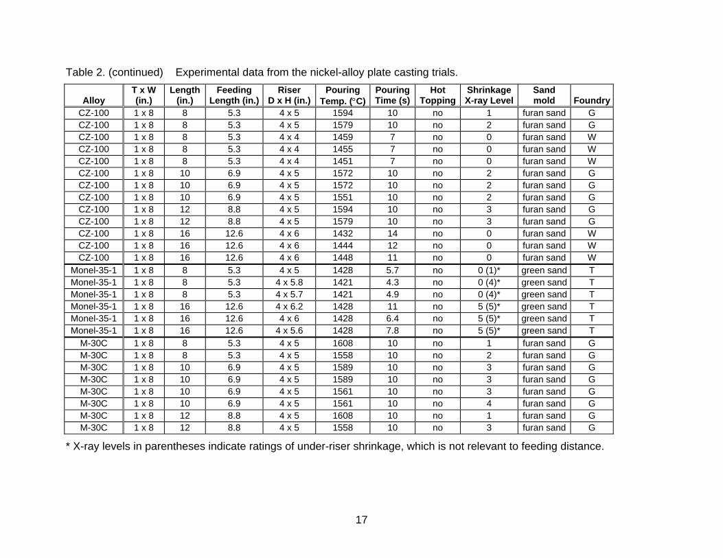
density, etc.) for these nickel alloys. For the C&LA and high alloy steels, a significant amount of property data was already available. This is not true for the present alloys. Property data was determined in the present work by coupling solidification temperature measurements of these alloys, taken during the casting trials, with property data computed from the software package JMatPro[6]. This package determines the solidification path and all casting-relevant material properties for a given alloy composition through thermodynamic calculations. The feeding distance development for these high-nickel alloys is currently well underway; this paper is intended to provide a progress report on the development. Section 2 describes the casting trials and provides the results of these trials. Section 3 describes the collection of thermocouple data during these casting trials that was necessary to develop property databases for the current alloys, and then Section 4 details the property database development for these alloys. Section 5 describes the casting simulations and presents the simulation results to date, and Section 6 discusses the current status and ongoing work in the project. 2. Casting Trials Five foundries participated in the nickel-alloy feeding distance trials. All foundries cast multiple lengths of 1 in. thick by 8 in. wide plates, using lengths chosen to produce plates ranging from completely sound to very unsound. A schematic of the general casting configuration is given in Figure 1. In terms of gating, this schematic is approximate; each foundry used a typical gating system for this type of casting. Trial data such as alloy composition, sand mold composition, pouring temperature and pouring time were collected during the trials, for later use in simulations. The alloy compositions measured during the casting trials are listed below each alloy’s nominal composition in Table 1. Note that the alloy M-30C appears in this table. This is because Foundry G cast M-30C rather than M-35-1; while these alloys are similar (compare the nominal compositions in Table 1), their resulting properties are different enough to warrant distinguishing between the alloys. Another important note regarding Table 1 is that the CW-12MW compositions cast by both Foundries N and G are out of specification. Foundry N has a molybdenum content that is slightly below specification, and Foundry G has both molybdenum and iron contents that are out of specification. In the latter case, the foundry ran out of pure molybdenum, and was forced to use charge metal containing both iron and molybdenum to raise the molybdenum content. After the plates were cast, the foundries had each plate examined using radiographic testing (RT) according to ASTM E94[7] procedures, using E446[8] reference radiographs (for casting sections up to 2 in. thick). Based on this examination, an ASTM shrinkage RT level was assigned to each plate. Table 2 lists the details for each plate cast by each foundry, including alloy, plate length, riser size, sand mold type, and resulting shrinkage x-ray level for the plate. Note that some plates have two shrinkage levels listed, with one in parentheses. In these cases, the first value is the shrinkage rating for the plate away from the riser, and the value in parentheses is a rating for the under-riser shrinkage. Because under-riser shrinkage is related to riser size and not feeding

3

distance, the under-riser ratings will not be used to develop feeding distance correlations. The experimental shrinkage RT results from the casting trials are presented in Figures 2 – 5. In each of these figures, the feeding length for each plate cast is plotted against its resulting ASTM shrinkage x-ray level. The feeding length (FL), shown schematically in Figures 2 – 5, is defined as the distance from the riser to the furthest point in the casting section being fed by that riser. The feeding length is purely geometrical; it should not be confused with the feeding distance (FD) defined in the introduction, which is the longest distance over which a riser can provide feed metal to produce a sound casting. In Figures 2 – 5, the hollow symbols represent the individual plates, with different symbols representing the different casting foundries. The numbers to the left of the hollow symbols indicate how many plates that symbol represents. The solid squares represent the average x-ray level for all plates with a given feeding length. The bold numbers to the right of these solid squares indicate their numerical value. The error bars associated with these squares indicate one standard deviation around the mean. Note that the mean and standard deviation values shown on these figures are not intended to provide valid statistical information; the number of plates at each feeding length is too small to provide any meaningful data. These are merely included to provide some indication about how the average x-ray levels change with feeding length, and to show the amount of scatter at a given feeding length. In these figures, notice that for a given foundry, the x-ray level tends to increase with feeding length. However, the x-ray levels for a given alloy seem to vary from foundry to foundry. This is currently being investigated. 3. Temperature Measurement As mentioned in the introduction, it was necessary to collect temperature data during the solidification of the alloys investigated in this work, in order to develop the property databases that would be used to simulate the casting trials. All temperature measurements were performed at A.G. Anderson, during their casting trials of the alloys CN-7M, CZ-100, CW-12MW and M-30C. Due to the high temperatures to which the thermocouples would be subjected during these trials (see Table 2), B-type thermocouples (Pt-6%Rh – Pt-30%Rh) were used. B-type thermocouples have a maximum operating temperature of about 3100°F (1700°C)[9]. The two types of thermocouple assemblies that were used are shown in Figure 6. In both arrangements, the thermocouple wire was encased in a two-hole high purity alumina ceramic insulating tube. In one arrangement, Figure 6a, the insulating tube was inserted into a closed-end fused quartz tube. In the other, Figure 6b, the insulating tube was inserted into a closed-end alumina ceramic protection tube, which was then inserted into an open-end fused quartz tube. In all thermocouple assemblies, the base end of the thermocouple (i.e., the end opposite the thermocouple bead) was sealed with a high-temperature alumina cement, to minimize convective and conductive heat losses. It should be noted that the original design of the thermocouple assemblies was the same as shown in Figure 6, but without the fused quartz tubes. A test of the original assemblies was performed at Keokuk Steel Castings, and all four of the thermocouples tested (two of each type shown in Figure 6) failed within one minute of pouring. Although there were

4

several possible reasons for failure, the most likely candidate was that thermal shock had cracked the alumina tubing and broken the thermocouple wires. To remedy this, fused quartz tubes were added to the remaining thermocouples that were to be taken to A.G. Anderson for the temperature measurements. Fused quartz is essentially immune to thermal shock (due to an extremely small thermal expansion coefficient), and it was thought that adding quartz tubes could prevent the thermocouple assemblies from being destroyed during the temperature measurement process. Schematics of the rigging used for the thermocouple plate trials are shown in Figure 7. Two plates, one 8 in. and one 12 in. long, were cast in each mold. For each alloy, one 12 in. plate was rigged with two thermocouples. Three thermocouples are shown in Figure 7a to indicate the three different possible thermocouple locations. This was necessary because there were three different sizes of thermocouples (see Figure 8):

• mid-plate thermocouple: the middle thermocouple in Figure 7a, that extends 5 in. into the plate, was 12 in. long and had an outer diameter (OD) of 0.394 in. (10 mm). This thermocouple had both an alumina protection tube and a fused quartz tube, as shown in Figure 6b.

• end-plate thermocouple (8 mm OD): the top thermocouple in Figure 7a, extending 0.5 in. into the plate, was 7.5 in. long and had an OD of 0.315 in. (8 mm). This thermocouple also had both an alumina protection tube and a fused quartz tube, as shown in Figure 6b. It was essentially a smaller version of the mid-plate thermocouple.

• end-plate thermocouple (6 mm OD): the bottom thermocouple in Figure 7a, extending 0.5 in. into the plate, was 7.5 in. long and had an OD of 0.236 in. (6 mm). This thermocouple had a fused quartz tube but no alumina protection tube, as shown in Figure 6a.

Each thermocoupled plate was cast with one mid-plate thermocouple, and one of the two end-plate thermocouples. The 6 mm OD end-plate thermocouples were used for CN-7M and CW-12MW, and the 8 mm OD end-plate thermocouples were used for CZ-100 and M-30C. To create holes in the mold into which the thermocouples could be inserted, holes of the appropriate size (6 mm, 8 mm or 10 mm) were drilled in both the side of the flask and the 12 in. plate pattern. Steel tubes of the same diameter as the corresponding thermocouples were inserted through the holes in the flask and into the holes in the plate pattern, and then the sand was poured into the flask and packed around these tubes. The tubes were then taken out so the mold could be removed from the flask, and then the thermocouples were inserted, as shown in Figure 9. The points where each thermocouple exited the mold were then covered in high temperature glue, to hold the thermocouples in place, prevent metal from exiting the mold, and to further limit convection and conduction heat losses. Before each alloy was poured, the two thermocouples were connected to a Personal Daq[10] portable data acquisition system. A measurement duration of 610 ms was used,

5

with an acquisition rate of 0.667 Hz. This provided the most accurate reading possible, and produced an output from each thermocouple every 1.5 seconds. The error inherent in a B-type thermocouple is about +/- 2 or 3°C[9]. The data acquisition was largely successful. Six of the eight thermocouples were completely successful in recording temperature data, while two thermocouples failed during solidification. The two that failed were in two different alloys, so at least one complete cooling curve was obtained for each alloy. Substantial data was obtained even for the two thermocouples that failed: in the CZ-100 trial, the 8 mm OD end-plate thermocouple failed after five minutes, and in the CW-12MW trial, the 10 mm mid-plate thermocouple failed after ten minutes. In both cases, the metal was mostly solidified when the thermocouples failed. The temperature data collected during these trials will be presented in the next section. 4. Property Database Development The temperature data recorded for each alloy was then used in conjunction with simulation to determine the material properties of each alloy before, during and after solidification. For each alloy, the measured composition was input into the software package JMatPro[6], which determines the solidification path and all casting-relevant material properties through thermodynamic calculations. Once these properties were calculated, they were input into the casting simulation software MAGMASOFT[11], and the thermocouple casting trials were simulated using the casting data collected during the trials. The thermocouples were included as a user-defined material in the MAGMASOFT simulations, and temperature and cooling rate versus time curves were output for various locations in the vicinity of the thermocouple beads. These predicted temperature and cooling rate curves were then compared with the measured curves, and adjustments to several aspects of the simulations were made to bring these curves into agreement, as described below. Plots showing the measured temperature and cooling rate curves together with the final simulated curves for each alloy are shown in Figures 10 – 13; these figures will be used to explain the adjustments that were made. The scale on the left of Figures 10 – 13 is for the temperature curves, while the scale on the right is for the cooling rate curves. Before comparing the measured and predicted temperatures, it is necessary to establish the liquidus (TL) and solidus (TS) temperatures, which denote the beginning and end of solidification, respectively, from the measured data. Both of these temperatures are obtained from the mid-plate thermocouple data (Figures 10a – 13a), because the end-plate thermocouples are subject to a significant conduction error, as explained in more detail below. The liquidus temperature is determined from a local peak in the cooling rate curve (see, for example, the left side of Figure 10a). Note that the cooling rate scale (right side of the plot in Figure 10a) increases from top to bottom, so this peak in the cooling rate curve is actually a local minimum in the cooling rate, caused by the onset of latent heat release as solidification begins. The liquidus temperature can also be seen as a kink in the temperature curve, from a very steeply descending slope to a much shallower slope (see the upper left of Figure 10a). For each of the four alloys, the minimum cooling rate corresponding to the liquidus

6

temperature is indicated by a vertical dashed line with arrows on each end in Figures 10a – 13a. The liquidus temperature is then given by the intersection of the vertical dashed line with the measured temperature curve, as indicated by a thick horizontal dashed line in the figures. The solidus temperature is determined from the measured cooling rate and temperature curves in a similar manner. At the location of the solidus, the cooling rate curve shows a local trough. Again, because the cooling rate scale on the right of these figures increases from top to bottom, a local trough is actually a local maximum in the cooling rate, brought about by the end of latent heat release at the end of solidification. For each of the four alloys, the maximum cooling rate corresponding to the solidus temperature is indicated by another vertical dashed line with arrows on each end in Figures 10a – 13a. The location of the maximum cooling rate is obvious for all alloys, except for CW-12MW (Figure 12a). This can be attributed to the mid-plate thermocouple in this casting failing prematurely. Nonetheless, it was possible to make a reasonable estimate of the location of the maximum cooling rate by checking the measured cooling rates for the end-plate thermocouple. The solidus temperature is now given by the intersection of the vertical dashed line with the measured temperature curve, as indicated by a thick horizontal dashed line in Figures 10 – 13. The measured liquidus and solidus temperatures are also summarized in Table 3. The estimated uncertainties in the measured liquidus and solidus temperatures are 3 oC and 10 oC, respectively. The first step in bringing the measured and simulated temperatures into agreement was to perform a time shift on the experimental data. The experimental time was shifted until the simulated and measured temperatures matched where the thermocouple reading first begins to decrease after its initial rise (see, for example, the upper left corner of Figure 10a). This time shift was necessary for two reasons. First, when the temperature measurements were taken, the data recorder was turned on a few minutes before pouring occurred, so the beginning of filling cannot be readily determined from the data. Second, there is a delay in thermocouple response time created by the insulating effect of the alumina and quartz tubes that protected the thermocouple beads. This explains why the mid-plate thermocouples, which were the largest thermocouples with the thickest insulating layers (10 mm OD quartz tubing), have longer time shifts than the end-plate thermocouples. The next step was to modify the thermal conductivity of the liquid metal in the simulation. This was done because the simulation neglects convection in the liquid. Convection enhances cooling of the liquid metal early in the casting process, before solidification begins. After some trial-and-error, the liquid metal thermal conductivity was multiplied by 2.5. This value was chosen because it brought the simulation cooling rate before solidification into agreement with the experimental data. This can be clearly seen on the far left sides of Figures 10 – 13 from the excellent agreement in the steeply decreasing temperatures before the liquidus is reached. Next, it was necessary to determine the effective thermal conductivity and other properties of the thermocouples themselves. The thermocouples were included in the casting simulations in order to model the effect of conduction losses on the

7

thermocouple readings. As shown in Figures 7 and 9, the thermocouples extended through the mold into the atmosphere, and it was noticed during the casting trials that the ends of the thermocouple tubes were glowing red hot. The heat conduction away from the thermocouple bead, along the tubes to the atmosphere, will generally result in readings that are lower than the metal temperature would be at the location of the bead. One indication of this effect can be seen for the end-plate thermocouple in Figures 10b and 12b: the measured end-plate temperatures never reach the liquidus temperature. There are many uncertainties involved in the thermal modeling of each thermocouple. The exact location of the thermocouple bead is not known, since the bead is inside a closed-end ceramic or quartz tube. Also, the thermal conductivity must account for many materials, including the ceramic insulators and tubes and the quartz tubes, as well as the air gaps present (see Figure 6). Finally, due to discretization limits in the simulation, the entire cross-section of the thermocouple must be represented by only a few control volumes, so it would be impossible to accurately represent the many materials that are in the thermocouple. Due to all of these complexities, it was decided that the best course of action would be to choose a single, effective thermal conductivity for the entire thermocouple arrangement. In addition, it was necessary to determine the location within the simulated thermocouple to assign to the thermocouple bead. This can be understood from the simulation grid arrangement inset into Figure 10a, for example. This picture shows part of the top-view cross-section that cuts through the middle of the plate and thermocouples. The top edge of this grid picture is the end of the plate, where the thermocouples are inserted. The long thermocouple that extends to the middle of the plate (mid-plate thermocouple) is on the left, and the short thermocouple that only extends a small distance into the plate (end-plate thermocouple) is on the right. Considering the mid-plate thermocouple, there are three cells (p2, p3 and p4) for which the temperatures predicted by the simulation are plotted in Figure 10a. The first cell, p2, is actually outside of the thermocouple (thus providing the actual metal temperature at this location), while p3 and p4 are both inside the thermocouple. Notice that these three predicted temperature curves are very similar, indicating that this region of the casting is relatively isothermal, and that conduction losses for the mid-plate thermocouples are small. On the other hand, the three predicted temperature curves for the end-plate thermocouple (at locations p8, p9 and p10 in Figure 10b) show differences of up to 30 oC at certain times. This indicates that the end-plate thermocouple is indeed experiencing significant conduction losses, as expected based on its location in the plate and the small amount of mold between the plate and the atmosphere. Based on this information, the end-plate thermocouple readings were used to determine the effective thermal conductivity. After some trial-and-error, a value of 10 W/m-K was selected for the effective thermal conductivity of the thermocouples, which seems realistic. Other, less important effective properties of the thermocouples were chosen as 2,700 kg/m3 for the density and 1,300 J/kg-K for the specific heat. Another adjustment that was required to obtain agreement in some instances was a slight adjustment to the composition. This was done in order to match the simulated liquidus temperatures from JMatPro with the measured values. Adjustment of the composition to obtain the measured liquidus temperature with JMatPro can be justified by the fact that there could be small inaccuracies in the measured compositions, that

8

there are local fluctuations in the composition away from the originally measured values (due to segregation, for example), and that there are some inaccuracies in the JMatPro thermodynamic database. For reference, the measured and adjusted compositions for the thermocouple trials are provided in Table 1. Care was taken to keep the adjustment amounts for each element as small as possible. The adjustments are not unique in that somewhat different adjustments could also produce agreement between the measured and predicted liquidus temperatures, but they are believed to be reasonable. In one instance, CN-7M, no adjustment was necessary, so the simulation composition is the same as that of Foundry G. For CZ-100, CW-12MW and M-30C, however, the simulation chemistry was adjusted from the Foundry G chemistry to obtain agreement. For CW-12MW, since the measured chemistries from Foundries G and N were significantly different (both were out of specification, but one was more so than the other), simulations for each of these casting trials used different chemistries. The chemistry given for the simulations for Foundry G is the chemistry adjusted from the measured values for Foundry G to match liquidus; the chemistry listed for the simulations for Foundry N are the same as the measured values for Foundry N. An example of the effect of adjusting the chemistry on the simulated liquidus temperature is shown for CZ-100 in Figure 14. Note that the curves generated with the adjusted chemistry match the measured liquidus temperature. Comparing the two curves labeled “2% cut-off”, it can be seen that the adjustment made to the composition of the CZ-100 alloy primarily causes a shift of the solid fraction versus temperature curve to lower temperatures, while preserving the general shape of the solidification path curve. Table 3 lists the liquidus temperatures predicted by JMatPro for both the measured and the adjusted compositions. A final adjustment was made in order to obtain agreement between the measured and predicted solidus temperatures. This was necessary because of the method used by JMatPro to model solidification. JMatPro employs a Scheil approach (infinitely fast diffusion in the liquid, no diffusion in the solid) for all elements except carbon and nitrogen, which are modeled with a lever rule approach (infinitely fast diffusion in both the liquid and solid). This is done because carbon and nitrogen are fast-diffusing elements in the solid. The use of this approach requires the definition of a solid fraction cut-off; if no cut-off is specified, the JMatPro approach produces a solidification path that asymptotically approaches a solid fraction of unity with decreasing temperature, but never actually reaches it. In addition, this cut-off can account for the formation of carbides or other phases when solidification is nearly complete. When a cut-off value is specified in JMatPro, say 2% for the sake of discussion, the simulation considers the material completely solidified when there is 2% liquid left (i.e., the material is 98% solidified). It then smoothes the end of solidification path, using a method not revealed to the user, so that it does not abruptly reach the solidus. An example of the effect that this has on the solidification path is seen in Figure 14, where the solidification path produced by two different cut-off values (2% and 8%) is shown. A number of cut-off values were tried for each of the adjusted alloy compositions, until the predicted solidus matched the measured solidus. Table 3 lists the cut-off values obtained in this manner, as well as the latent heat values, for each alloy. For the base-line JMatPro simulations with the measured compositions, an arbitrary cut-off value of 2% is always used. For

9

the adjusted compositions, the cut-off value reflects the matching of the measured and predicted solidus temperatures, as explained above. It can be seen that the cut-off values range from 2% to 15% and that the different cut-offs shift the solidus temperature by up to 150 oC. The higher cut-off values cause significant changes in the solidification path that are unlikely to be very realistic. Nonetheless, it was decided that for the purposes of the present study it is more important to match the measured and predicted solidus temperatures than to attain an accurate solidification path. Since the cut-off value for M-30C is only 2%, this solidification path is likely to be quite accurate. The final property curves predicted by JMatPro and used in the simulation of the casting trials are summarized for CN-7M, CZ-100, CW-12MW, M-35-1 and M-30C in Figures 15 – 18. These curves were generated using the chemistries labeled as “Simulation” in Table 1. In the case of CW-12MW, the curves shown in Figures 15 – 18 are for the Foundry N chemistry, since the Foundry G chemistry is notably out of specification. The solid fraction curves for these alloys are shown in Figure 15. This figure demonstrates why M-35-1 and M-30C were treated separately; although they have nearly the same liquidus and similar solidus temperatures, they have very different solidification paths. Figure 16 contains the density curves for these alloys. All of the nickel-base alloys have similar density curves. The CN-7M curve is of a similar shape, but the density is lower at any given temperature than for the nickel-base alloys. The thermal conductivity curves are provided in Figure 17. The CN-7M and the CW-12MW curves are very similar. The remaining nickel-base alloys have conductivity curves that are also similar to each other, but with significantly higher conductivity values than CN-7M and CW-12MW. Finally, the specific heat curves are shown in Figure 18. These curves are all relatively similar. Returning now to Figures 10 – 13, generally good agreement can be observed between the measured and predicted temperatures and cooling rates for both the mid-plate and the end-plate thermocouples. The mid-plate thermocouple comparisons (Figure 10a – 13a) show small deviations between the measured and predicted temperatures that occur between the liquidus and solidus temperatures, near the end of solidification. These deviations can be attributed to the use of relatively high cut-off values in some cases to achieve agreement between the measured and predicted solidus temperatures, as explained previously (Table 3). The change in the solidification path produced by the cut-off (see Figure 14) causes the latent heat release in the simulation to be inaccurate. It would have been possible to make further, “manual” adjustments to the solidification path for each of the alloys (Figure 15), but this would have meant abandoning the use of JMatPro for obtaining the material properties altogether. The end-plate thermocouple comparisons (Figure 10b – 13b) are also good other than that the conduction error appears to be underestimated for two of the casting trials (Figures 10b and 13b). Further adjustments to the end-plate thermocouple effective thermal conductivity used in the simulations would have been possible, but the present choice appears to produce reasonable overall agreement for most casting trials. Note from Figure 12b that the accounting for the conduction error in the simulations, through the inclusion of the thermocouples, is able to approximately reproduce the measured effect that the end-plate thermocouple does not reach the liquidus temperature.

10

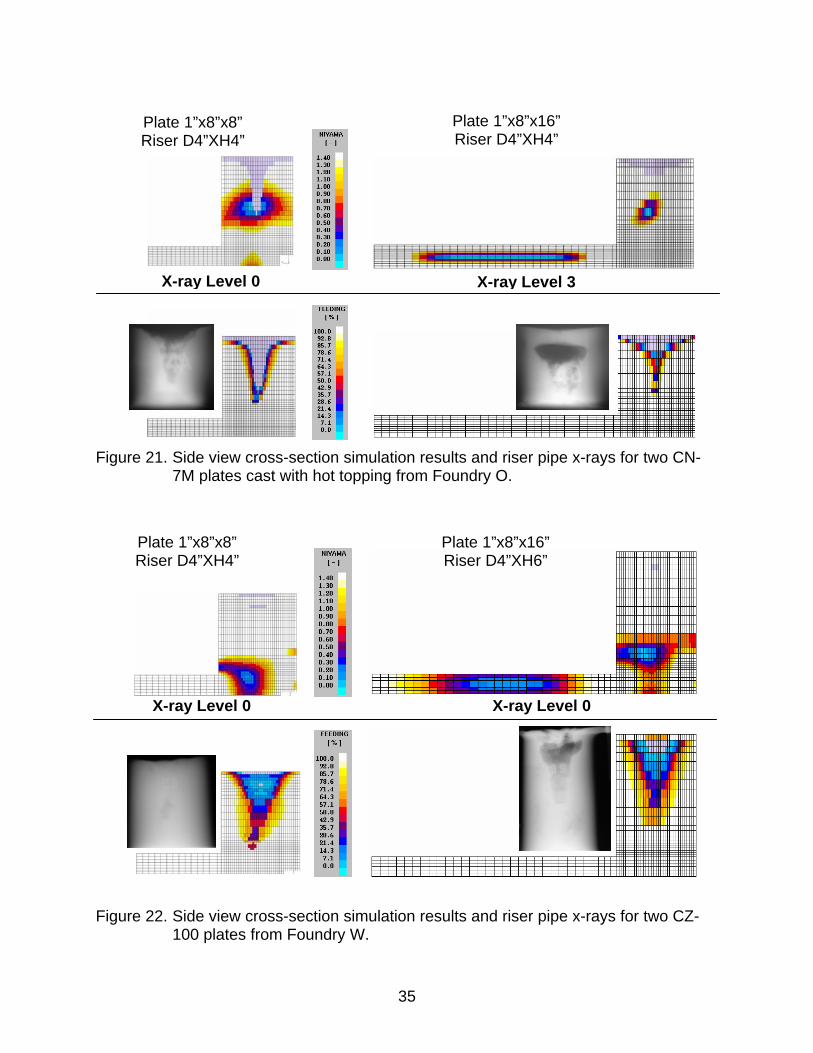
5. Casting Trial Simulations Based on the information collected during the plate casting trials, and using the material property data for each alloy described in the previous section, MAGMASOFT simulations were performed for each plate listed in Table 2 for which unique casting data is available. Special care was taken to specify a realistic thermal boundary condition at the top of the riser for those cases where no hot topping was used (Table 2). In MAGMASOFT, the default boundary condition at the top of the riser corresponds to the use of hot topping. The simulations of the plate casting trials provide the distribution of the Niyama criterion as well as the feeding percentage throughout the castings. The Niyama criterion[12] is a local thermal parameter defined as TG &/ [K1/2s1/2mm-1], where G is the temperature gradient and T& is the cooling rate[2]. The feeding percentage represents the amount of each control volume that contains solid metal; it is equal to one minus the porosity percentage. Due to limitations of the feeding algorithm currently used in MAGMASOFT, no feeding percentages are predicted along the centerline inside the plates, away from the riser, even if a large amount of porosity is revealed by the x-rays (see figures below)[2,3]. Therefore, the feeding percentages are only used to compare simulated and measured riser pipes. The correlation between the x-ray indications inside the plate and the simulation results must rely on the Niyama criterion. Generally, a smaller Niyama value corresponds to a higher probability of porosity occurring in the plate. Our previous work on C&LA and high alloy steels[2-4] indicated a critical Niyama value of 0.1 below which porosity indications become visible on an x-ray film such that a level of 1 or greater would be assigned. The following comparisons between predicted Niyama values (and feeding percentages) and shrinkage indications and levels from x-rays are intended to shed some light on this correspondence between simulation and casting trials for the present high-nickel alloys. Figure 19 shows simulation and x-ray results from two of the CN-7M plates cast at Foundry O. The upper panels show the Niyama values together with the measured x-ray levels. It can be seen that for the short plate (left side) there is no Niyama indication below 1.4 other than for a small indication in the riser; the measured x-ray level for this plate is 0 (i.e., completely sound). For the longer plate (right side), a large region with Niyama values below 0.1 can be observed along the centerline; the measured x-ray level for this plate is 3. The lower panels show the predicted feeding percentages together with x-rays of the un-cut risers and photographs of the cut risers. For these plates, no hot topping was used. It can be seen that the riser is frozen off at the top and that the riser pipe consists of an internal shrinkage cavity. For both plates, good agreement exists between the predicted riser pipes and what can be discerned from the x-rays and photographs. Figure 20 shows top views, cut at the mid-plate thickness, of the predicted Niyama values for the same two plates, together with the top-view x-ray of the longer plate. For the longer plate, a good correlation can be observed between the shrinkage indications on the x-ray and the region where Niyama values below approximately 0.1 are predicted. Since the shorter plate is radiographically sound (x-ray level 0), no image of the x-ray is included in Figure 20. All predicted Niyama values for this plate are above 1.4. Figure 21 shows a comparison of the predicted feeding

11

percentages and Niyama values with riser x-rays for two plates of the same alloy and dimensions as in Figures 19 and 20, but for a case where a hot topping was used. For the shorter plate (left side) excellent agreement exists between the predicted feeding percentages and the riser pipe indications on the x-ray. Note that the hot topping caused the riser pipe to be open at the top. For the longer plate, the agreement is not as good, primarily because the hot topping does not appear to have been effective in the casting trial; a thick solid layer can be observed on the x-ray at the top of the riser, and the riser pipe consists of an internal shrinkage cavity, as if no hot topping was applied. Figure 22 shows similar results for two plates made of CZ-100. No Niyama indications below 1.4 are predicted for the shorter plate other than inside and right below the riser. The measured x-ray level for this plate is 0 (completely sound). For the longer plate, a fairly large region of Niyama values below 1.4 is predicted inside the plate, but all Niyama values are above 0.2. No internal shrinkage indications are apparent on the x-ray for this plate, as indicated on the figure (x-ray level 0). The riser pipes are reasonably well predicted by the feeding percentages for both the short and the long plate (lower panels of Figure 22). No hot topping was used. For the shorter plate, the internal riser pipe on the x-ray appears smaller than what is predicted. This could be attributed to the presence of a depression at the top of the riser on the x-ray that is not predicted in the present simulation. It is possible that an adjustment in the thermal boundary conditions at the top of the riser would produce better agreement for this riser. The predicted Niyama distributions for two CW-12MW plates are compared to the corresponding top-view x-rays in Figure 23 (no riser x-rays are available for these plates). Both plates show a shrinkage indication directly below the riser, while the Niyama values in this region are all above 1.4. This discrepancy can be attributed to the simulation predicting a riser pipe that is shorter than the pipe the casting trials produced. The shorter plate itself, away from the riser, is radiographically sound (x-ray level 0) and all Niyama values are above 1.4. The longer plate has level 4 indications along the centerline, extending almost throughout the length of the plate. The predicted Niyama values below 1.4 approximately coincide with this shrinkage pattern. The minimum Niyama values inside the longer plate are below 0.1. Figures 24 and 25 show the predicted Niyama and feeding percentage distributions and the corresponding x-rays for two M-35-1 plates. Good agreement can be observed between the feeding percentages and the riser pipes on the x-rays (lower panels in Figure 24), although the depth of the riser pipe for the shorter plate is somewhat over predicted. The Niyama predictions also show a good correspondence with the x-rays, as can be seen in Figure 25. The short plate has a level 4 indication below the riser that coincides with Niyama values between about 0.4 and 1.0. The remainder of the plate is radiographically sound (x-ray level 0) and all Niyama values are above 1.4. The longer plate has several level 5 indications along the centerline on the top-view x-ray. These correspond very well with the predicted Niyama values at the same locations. The minimum Niyama value in the level 5 region is about 0.1.

12

Figure 26 plots the predicted minimum Niyama values for all casting trial plates as a function of the feeding length of the plates. Here, ‘feeding length’ should not be confused with ‘feeding distance’; the feeding length is simply the length to be fed, as explained in the inset in Figure 26. Even though the results correspond to five different high-Ni alloys, the minimum Niyama values show the same trend: they decrease with increasing feeding length length. A very similar trend was observed in our previous studies on C&LA and high alloy steels[2-4], but a direct comparison cannot be made because the plate lengths and W/T ratios were different. The longer plates typically have a higher x-ray rating level, while the shortest plates are usually sound. This indicates that the Niyama criterion can be used as an indicator of soundness and as a tool to determine feeding distances. A plot of the measured x-ray levels versus the predicted minimum Niyama values is not included in this paper, because some of the x-ray ratings still needed to be verified at the time of writing. 6. Conclusions A total of 55 plates of varying length were cast at five foundries in an effort to develop feeding distance rules for the nickel-based alloys CZ-100, M-35-1 and CW-12MW, as well as for the austenitic stainless steel CN-7M. In order to develop the property databases necessary to simulate these alloys, temperature data was recorded for each alloy during the casting trials. This measured data was then used in conjunction with material property simulation (JMatPro) to develop the necessary property data for each alloy. This paper documents the property data obtained, and foundries interested in using them should contact the authors. A comparison of the radiographs taken of the plates and the risers with the corresponding MAGMASOFT casting simulation results reveals generally good agreement. The riser pipes correlate well with the feeding percentage predictions in MAGMASOFT, while the shrinkage indications on the x-rays for those plates where the feeding distance was exceeded are well predicted by the Niyama criterion. The study will be completed within the next few months by first establishing a direct, quantitative correlation between the measured x-ray levels and the predicted minimum Niyama values. Then, a large number of additional simulations will be conducted to establish general feeding and risering rules. The rules will be tailored to the alloy composition, casting conditions and geometry, and soundness desired, as in our previous C&LA and high alloy steel work[2-4]. Acknowledgements This work was prepared with the support of the U.S. Department of Energy (DOE) Award No. DE-FC36-02ID14225. However, any opinions, findings, conclusions, or recommendations expressed herein are those of the authors, and do not necessarily reflect the views of the DOE. We are indebted to Malcolm Blair and Raymond Monroe of the SFSA for their work in helping organize the trials and recruiting members to participate. Most importantly, we thank the participants in the plate casting trials (A.G. Anderson, Ancast, Southern Alloy, Stainless Foundry & Engineering, and Wollaston

13

Alloy) for their substantial investments of both time and resources. This work could not have been accomplished without their shared efforts. In particular, we are very grateful to Vasile Ionescu of A.G. Anderson, for his help in organizing, preparing for, and performing the thermocouple casting trials. References 1. Risering Steel Castings, Steel Founders' Society of America, Barrington, Illinois,

1973. 2. K.D. Carlson, S. Ou, R.A. Hardin and C. Beckermann: “Development of New

Feeding-Distance Rules Using Casting Simulation: Part I. Methodology,” Metall. Mater. Trans. B, 2002, vol. 33B, pp. 731-740.

3. S. Ou, K.D. Carlson, R.A. Hardin and C. Beckermann: “Development of New Feeding-Distance Rules Using Casting Simulation: Part II. The New Rules,” Metall. Mater. Trans. B, 2002, vol. 33B, pp. 741-755.

4. Feeding & Risering Guidelines for Steel Castings, Steel Founders' Society of America, Barrington, Illinois, 2001.

5. K.D. Carlson, S. Ou and C. Beckermann: “Feeding and Risering of High Alloy Steel Castings,” 2003 SFSA Technical and Operating Conference, 2003.

6. JMatPro, Sente Software Ltd., Surrey Technology Centre, 40 Occam Road, GU2 7YG, United Kingdom.

7. ASTM E94-00, Annual Book of ASTM Standards, Volume 03.03: Nondestructive Testing, American Society for Testing and Materials, 2002.

8. ASTM E446-98, Annual Book of ASTM Standards, Volume 03.03: Nondestructive Testing, American Society for Testing and Materials, 2002.

9. Manual on the Use of Thermocouples in Temperature Measurement, ASTM Special Technical Publication 470B, American Society for Testing and Materials, 1981.

10. Personal Daq, IOTech, Inc., 25971 Cannon Road, Cleveland, Ohio 44146, USA. 11. MAGMASOFT, MAGMA GmbH, Kackerstrasse 11, 52072 Aachen, Germany. 12. E. Niyama, T. Uchida, M. Morikawa and S. Saito: Am. Foundrymen’s Soc. Int. Cast

Met. J., 1982, vol. 7 (3), pp. 52-63.

14

15

Table 1. Compositions for the alloys of interest, given in weight percent. Nominal composition entries that are single numbers rather than number ranges indicate the maximum weight percentage for that element.

Alloy C Mn Si P S Cr Ni Cu Mo Cb W V Fe

Nominal 0.07 1.5 1.5 0.04 0.04 19 -22 27.5 -30.5 3 - 4 2 - 3 balance

Foundry G 0.019 0.76 0.34 0.023 0.01 19 27.54 3.9 2.1 46.3

Foundry O 0.05 0.59 0.57 0.015 0.025 20.5 28.6 3.51 2.26 43.88 CN-7M

Simulation 0.019 0.76 0.34 0.023 0.01 19 27.54 3.9 2.1 46.3

Nominal 1 1.5 2 0.03 0.03 balance 1.25 3 Foundry W 0.735 0.869 1.57 0.001 0.003 96.5 0.057 0.265 Foundry G 0.76 0.46 0.79 0.001 0.006 97.29 0.01 0.68 CZ-100

Simulation 0.86 1.5 0.89 0.06 0.01 94 1.2 1.48

Nominal 0.12 1 1 0.04 0.03 15.5 - 17.5 balance 16 - 18 3.75 -

5.25 0.2 - 0.4 4.5 - 7.5

Foundry G 0.03 0.2 0.54 0.029 0.018 15.6 52.78 15.2* 3.77 0.23 11.6* Simulation

(for G) 0.04 0.3 0.7 0.02 0.03 15.6 52.6 16 3.77 0.23 10.7*

Foundry N 0.06 0.67 0.76 0.005 0.015 17.3 55.25 15.8* 4.1 0.24 5.8

CW-12MW

Simulation (for N) 0.06 0.67 0.76 0.005 0.015 17.3 55.25 15.8* 4.1 0.24 5.8

Nominal 0.3 1.5 1 - 2 0.03 0.03 0.03 balance 26 - 33 1 - 3 3.5 Foundry G 0.02 1.07 1.54 0.001 0.005 60.72 31.95 1.3 3.4 M-30C

Simulation 0.12 1.07 1.54 0.001 0.005 60.72 32 1.3 3.4 Nominal 0.35 1.5 1.25 0.03 0.03 balance 26 - 33 0.5 3.5

Foundry T 0.181 1.129 1.035 0.0047 0.004 0.3 64.58 30.88 0.005 0.03 1.87 M-35-1

Simulation 0.181 1.129 1.035 0.0047 0.004 0.3 64.58 30.88 0.005 0.03 1.87

* Note: entries listed in red are out of specification.

16

Table 2. Experimental data from the nickel-alloy plate casting trials.

Alloy T x W (in.)

Length (in.)

Feeding Length (in.)

Riser D x H (in.)

Pouring Temp. (°C)

Pouring Time (s)

Hot Topping

Shrinkage X-ray Level

Sand mold

Foundry

CN-7M 1 x 8 8 5.3 4 x 5 1608 10 no 2 furan sand G CN-7M 1 x 8 8 5.3 4 x 5 1558 10 no 2 furan sand G CN-7M 1 x 8 8 5.3 4 x 4 1496 7 no 0 furan sand O CN-7M 1 x 8 8 5.3 4 x 4 1492 7 no 0 furan sand O CN-7M 1 x 8 8 5.3 4 x 4 1487 7 no 0 furan sand O CN-7M 1 x 8 8 5.3 4 x 4 1496 7 yes 0 furan sand O CN-7M 1 x 8 10 6.9 4 x 5 1589 10 no 2 furan sand G CN-7M 1 x 8 10 6.9 4 x 5 1589 10 no 3 furan sand G CN-7M 1 x 8 10 6.9 4 x 5 1561 10 no 3 furan sand G CN-7M 1 x 8 10 6.9 4 x 5 1561 10 no 3 furan sand G CN-7M 1 x 8 12 8.8 4 x 5 1608 10 no 5 furan sand G CN-7M 1 x 8 12 8.8 4 x 5 1558 10 no 5 furan sand G CN-7M 1 x 8 16 12.6 4 x 4 1496 10 no 4 furan sand O CN-7M 1 x 8 16 12.6 4 x 4 1492 10 no 3 furan sand O CN-7M 1 x 8 16 12.6 4 x 4 1487 10 no 2 furan sand O CN-7M 1 x 8 16 12.6 4 x 4 1496 10 yes 3 furan sand O

CW-12MW 1 x 8 8 5.3 4 x 5 1584 10 no 2 furan sand G CW-12MW 1 x 8 8 5.3 4 x 5 1521 10 no 3 furan sand G CW-12MW 1 x 8 8 5.3 4 x 4 1588 4 no 0 (3)* furan sand N CW-12MW 1 x 8 8 5.3 4 x 4 1579 4 no 0 (3)* furan sand N CW-12MW 1 x 8 8 5.3 4 x 4 1571 4 no 0 (3)* furan sand N CW-12MW 1 x 8 10 6.9 4 x 5 1558 10 no 2 furan sand G CW-12MW 1 x 8 10 6.9 4 x 5 1558 10 no 3 furan sand G CW-12MW 1 x 8 12 8.8 4 x 5 1584 10 no 4 furan sand G CW-12MW 1 x 8 12 8.8 4 x 5 1521 10 no 5 furan sand G CW-12MW 1 x 8 16 12.6 4 x 4 1560 7 no 2 (3)* furan sand N CW-12MW 1 x 8 16 12.6 4 x 4 1552 8 no 2 (3)* furan sand N CW-12MW 1 x 8 16 12.6 4 x 4 1541 9 no 4 (4)* furan sand N

* X-ray levels in parentheses indicate ratings of under-riser shrinkage, which is not relevant to feeding distance.

17

Table 2. (continued) Experimental data from the nickel-alloy plate casting trials.

Alloy T x W (in.)

Length (in.)

Feeding Length (in.)

Riser D x H (in.)

Pouring Temp. (°C)

Pouring Time (s)

Hot Topping

Shrinkage X-ray Level

Sand mold

Foundry

CZ-100 1 x 8 8 5.3 4 x 5 1594 10 no 1 furan sand G CZ-100 1 x 8 8 5.3 4 x 5 1579 10 no 2 furan sand G CZ-100 1 x 8 8 5.3 4 x 4 1459 7 no 0 furan sand W CZ-100 1 x 8 8 5.3 4 x 4 1455 7 no 0 furan sand W CZ-100 1 x 8 8 5.3 4 x 4 1451 7 no 0 furan sand W CZ-100 1 x 8 10 6.9 4 x 5 1572 10 no 2 furan sand G CZ-100 1 x 8 10 6.9 4 x 5 1572 10 no 2 furan sand G CZ-100 1 x 8 10 6.9 4 x 5 1551 10 no 2 furan sand G CZ-100 1 x 8 12 8.8 4 x 5 1594 10 no 3 furan sand G CZ-100 1 x 8 12 8.8 4 x 5 1579 10 no 3 furan sand G CZ-100 1 x 8 16 12.6 4 x 6 1432 14 no 0 furan sand W CZ-100 1 x 8 16 12.6 4 x 6 1444 12 no 0 furan sand W CZ-100 1 x 8 16 12.6 4 x 6 1448 11 no 0 furan sand W

Monel-35-1 1 x 8 8 5.3 4 x 5 1428 5.7 no 0 (1)* green sand T Monel-35-1 1 x 8 8 5.3 4 x 5.8 1421 4.3 no 0 (4)* green sand T Monel-35-1 1 x 8 8 5.3 4 x 5.7 1421 4.9 no 0 (4)* green sand T Monel-35-1 1 x 8 16 12.6 4 x 6.2 1428 11 no 5 (5)* green sand T Monel-35-1 1 x 8 16 12.6 4 x 6 1428 6.4 no 5 (5)* green sand T Monel-35-1 1 x 8 16 12.6 4 x 5.6 1428 7.8 no 5 (5)* green sand T

M-30C 1 x 8 8 5.3 4 x 5 1608 10 no 1 furan sand G M-30C 1 x 8 8 5.3 4 x 5 1558 10 no 2 furan sand G M-30C 1 x 8 10 6.9 4 x 5 1589 10 no 3 furan sand G M-30C 1 x 8 10 6.9 4 x 5 1589 10 no 3 furan sand G M-30C 1 x 8 10 6.9 4 x 5 1561 10 no 3 furan sand G M-30C 1 x 8 10 6.9 4 x 5 1561 10 no 4 furan sand G M-30C 1 x 8 12 8.8 4 x 5 1608 10 no 1 furan sand G M-30C 1 x 8 12 8.8 4 x 5 1558 10 no 3 furan sand G

* X-ray levels in parentheses indicate ratings of under-riser shrinkage, which is not relevant to feeding distance.

18

Table 3. Simulated and measured values of liquidus and solidus temperatures, with simulated values of latent heat.

Solidus

Alloy Liquidus

TL (ºC) TS (ºC) Solidification

cut-off (%) Latent heat

(J/g) Measurement – thermocouple data 1392.5 1300

JMatPro: Measured G composition 1392.5 1151 2 195.9 CN-7M

JMatPro: Adjusted G composition 1392.5 1300 15 174.3

Measurement – thermocouple data 1376.9 1243 JMatPro: Measured G composition 1402.2 1274 2 268 CZ-100 JMatPro: Adjusted G composition 1376.9 1243 8 238

Measurement – thermocouple data 1359.5 1207

JMatPro: Measured G composition 1369.5 990 2 220

JMatPro: Adjusted G composition 1359.5 1207 11 191.6 CW-12MW

JMatPro: Measured N composition 1350 1206 11 191.8

Measurement – thermocouple data 1303.1 1192.6

JMatPro: Measured G composition 1312.5 1178 2 205 M-30C

JMatPro: Adjusted G composition 1303.1 1192.6 2 195

M-35-1 JMatPro: Measured T composition 1303.6 1196 2 198

19

Figure 1. General configuration for the nickel-alloy plate casting trials.

riser

casting

gating drag

T

cope HR

W

mold

FL DR

L

side-view cross section

top-view cross section

20

Figure 2. Casting trial results: feeding length versus shrinkage x-ray level for CN-7M plates.

0.67

2.75 2.75

5

-1

0

1

2

3

4

5

6

0 2 4 6 8 10 12 14

Feeding Length, FL (in.)

AST

M S

hrin

kage

X-r

ay L

evel

Foundry G (8 plates)Foundry O (8 plates)Mean X-ray Level +/- 1 Standard Deviation

D W

FL

L

W/T = 8

CN-7M (16 plates total)

4

2 1 2

3 1

1

2

21

Figure 3. Casting trial results: feeding length versus shrinkage x-ray level for CZ-100 plates.

0

3

2

0.6

-1

0

1

2

3

4

5

6

0 2 4 6 8 10 12 14


AST

M S

hrin

kage

X-r

ay L

evel

Foundry G (7 plates)

Foundry W (6 plates)Mean X-ray Level +/- 1 Standard Deviation

D W

FL

L

W/T = 8

CZ-100 (13 plates total)

33

1

1 3

2

22

Figure 4. Casting trial results: feeding length versus shrinkage x-ray level for CW-12MW plates.

4.5

2.5

1

2.67

-1

0

1

2

3

4

5

6

0 2 4 6 8 10 12 14


AST

M S

hrin

kage

X-r

ay L

evel

Foundry G (6 plates)

Foundry N (6 plates)

Mean X-ray Level +/- 1 Standard Deviation

DR

WFL

L

W/T = 8

CW-12MW (12 plates total)

3

1 1 2

1 1

1 1

1

23

Figure 5. Casting trial results: feeding length versus shrinkage x-ray level for Monel-35-1 and M-30C plates.

0.6

1.5

5

3.25

-1

0

1

2

3

4

5

6

0 2 4 6 8 10 12 14


AST

M S

hrin

kage

X-r

ay L

evel

Foundry G, M-30C (8 plates)Foundry T, M-35-1 (6 plates)Mean X-ray Level +/- 1 Standard Deviation

D W

FL

L

W/T = 8

M-30C & Monel-35-1 (14 plates total)

3

1 1

1 1

3

1

3

24

Figure 6. Cross-sectional schematics of thermocouple assemblies (a) without an

alumina protection tube, and (b) with an alumina protection tube.

(a)

(b)

fused quartz 2-hole alumina insulator

alumina protection tube

B-type thermocouple wire

thermocouple bead

25

Figure 7. Schematics of the rigging used for the thermocouple trials.

(b) side view

HR = 5”

T = 1”

10 ppi filter

(a) top view

DR = 4”

L = 8”

W = 8” (both plates)

DR = 4”

L = 12”

thermocouples (2 of these 3 used for each plate)

1.5” 1.5”

5”

0.5”

D = 3”

3”

26

Figure 8 Picture of the three different thermocouples used in the trials. Figure 9 Mold cope, with two thermocouples inserted.

mid-plate thermocouple (10 mm OD)

end-plate thermocouple 1 (8 mm OD)

end-plate thermocouple 2 (6 mm OD)

27

700

800

900

1000

1100

1200

1300

1400

1500

0 400 800 1200 1600 2000 2400 2800

Time, s

Tem

pera

ture

, ºC

-1.5

-1

-0.5

0

0.5

1

Coo

ling

rate

, ºC

/s

TL = 1376.9 ºC

TS = 1243 ºC

MeasurementSimulation at p2Simulation at p3 Simulation at p4

-1

-0.5

0

0.5

1.0

1.5

CZ-100mid-plate thermocouple

(TC time delay 26s)

700

800

900

1000

1100

1200

1300

1400

1500

0 400 800 1200 1600 2000 2400 2800

Time, s

Tem

pera

ture

, ºC

-1.5

-1

-0.5

0

0.5

1

Coo

ling

rate

, ºC

/s

CZ-100end-plate thermocouple

(TC time delay 22s)


TL = 1376.9 ºC

TS = 1243 ºC

TC failure

-1

-0.5

0

0.5

1.0

1.5

(a)

(b)

Figure 10. Measured and simulated CZ-100 temperature and cooling rate curves for (a) mid-plate thermocouple (TC); and (b) end-plate TC.

28

700

800

900

1000

1100

1200

1300

1400

1500

0 400 800 1200 1600 2000 2400

Time, s

Tem

pera

ture

, ºC

-1.5

-1

-0.5

0

0.5

1

Coo

ling

rate

, ºC

/s


TL = 1392.5 ºC

TS = 1300 ºC

-1

-0.5

0

0.5

1.0

1.5

CN-7Mmid-plate thermocouple

(TC time delay 32s)

700

800

900

1000

1100

1200

1300

1400

1500

0 400 800 1200 1600 2000 2400

Time, s

Tem

pera

ture

, ºC

-1.5

-1

-0.5

0

0.5

1

Coo

ling

rate

, ºC

/s

CN-7Mend-plate thermocouple

(TC time delay 6s)


TL = 1392.5 ºC

TS = 1300 ºC

-1

-0.5

0

0.5

1.0

1.5

(a)

(b)

Figure 11. Measured and simulated CN-7M temperature and cooling rate curves for (a) mid-plate thermocouple (TC); and (b) end-plate TC.

29

700

800

900

1000

1100

1200

1300

1400

1500

0 400 800 1200 1600 2000

Time, s

Tem

pera

ture

, ºC

-1.5

-1

-0.5

0

0.5

1

Coo

ling

rate

, ºC

/s

TL = 1359.5 ºC


TC failure

-1

-0.5

0

0.5

1.0

1.5

TS = 1207 ºC

CW-12MWend-plate thermocouple

(TC time delay 30s)

700

800

900

1000

1100

1200

1300

1400

1500

0 400 800 1200 1600 2000

Time, s

Tem

pera

ture

, ºC

-1.5

-1

-0.5

0

0.5

1

Coo

ling

rate

, ºC

/s

CW-12MWend-plate thermocouple

(TC time delay 10s)

TL= 1359.5 ºC

TS = 1207 ºC


TC failure

-1

-0.5

0

0.5

1.0

1.5

Figure 12. Measured and simulated CW-12MW temperature and cooling rate curves for

(a) mid-plate thermocouple (TC); and (b) end-plate TC.

(b)

(a)

30

700

800

900

1000

1100

1200

1300

1400

1500

0 400 800 1200 1600 2000 2400 2800

Time, s

Tem

pera

ture

, ºC

-1.5

-1

-0.5

0

0.5

1

Coo

ling

rate

, ºC

/s


TL = 1303.1 ºC

TS = 1192.6 ºC

-1

-0.5

0

0.5

1.0

1.5

M-30Cmidd-plate thermocouple

(TC time delay 30s)

700

800

900

1000

1100

1200

1300

1400

1500

0 400 800 1200 1600 2000 2400 2800

Time, s

Tem

pera

ture

, ºC

-1.5

-1

-0.5

0

0.5

1

Coo

ling

rate

, ºC

/s

MeasurementSimulation at p8Simulation at p9 Simulation at p10 TL = 1303.1 ºC

TS = 1192.6 ºC

-1

-0.5

0

0.5

1.0

1.5

M-30Cend-plate thermocouple

(TC time delay 5s)

(a)

(b)

Figure 13. Measured and simulated M-30C temperature and cooling rate curves for (a) mid-plate thermocouple (TC); and (b) end-plate TC.

31

0

0.1

0.2

0.3

0.4

0.5

0.6

0.7

0.8

0.9

1

1100 1125 1150 1175 1200 1225 1250 1275 1300 1325 1350 1375 1400

Temperature, ºC

Solid

frac

tion

Foundry G adjusted chemistry

2% cut-off

8% cut-off

FoundryG original chemistry

CZ-100Measured liquidus temperture

TL = 1376.9 ºC

Figure 14. Variations in the simulated solidification path for CZ-100 due to changes in

the metal chemistry and the simulation cut-off percentage.

0

0.1

0.2

0.3

0.4

0.5

0.6

0.7

0.8

0.9

1

1150 1200 1250 1300 1350 1400

Temperature, ºC

Solid

frac

tion

CN-7M

CW-12MW(N composition)

CZ-100

M-35-1

M-30C

Figure 15. Simulated solid fraction curves.

32

7000

7200

7400

7600

7800

8000

8200

8400

8600

8800

9000

0 200 400 600 800 1000 1200 1400 1600

Temperature, ºC

Den

sity

, kg/

m3

M-35-1


CZ-100

CN-7M

M-30C

Figure 16. Simulated density curves.

0

10

20

30

40

50

60

70

80

90

0 200 400 600 800 1000 1200 1400 1600

Temperature, ºC

Ther

mal

Con

duct

ivity

, W/(m

K)

M-35-1


CZ-100

CN-7M

M-30C

Figure 17. Simulated thermal conductivity curves.

33

0

100

200

300

400

500

600

700

800

0 200 400 600 800 1000 1200 1400 1600

Temperature, ºC

Spec

ific

Hea

t, J/

(kgK

)


CN-7M

CZ-100

M-35-1 & M-30C

Figure 18. Simulated specific heat curves.

Figure 19. Side view cross-section simulation results and riser pipe x-rays for two CN-

7M plates from Foundry O.

X-ray Level 3 X-ray Level 0

Plate 1”x8”x16” Riser D4”XH4”


34

Figure 20. Top view cross-section simulation results for two CN-7M plates from Foundry

O, with plate x-ray for long plate.

X-ray Level 3

X-ray Level 0



35

Figure 21. Side view cross-section simulation results and riser pipe x-rays for two CN-

7M plates cast with hot topping from Foundry O. Figure 22. Side view cross-section simulation results and riser pipe x-rays for two CZ-

100 plates from Foundry W.







36

Figure 23. Top view cross-section simulation results for two CW-12MW plates from

Foundry N, shown with corresponding plate x-rays.

Figure 24. Side view cross-section simulation results and riser pipe x-rays for two M-35-

1 plates from Foundry T.


X-ray Level 4 (4) X-ray Level 0 (3)



Plate 1”x8”x8” Riser D4”XH5.7”


37

Figure 25. Top view cross-section simulation results for two M-35-1 plates from Foundry

T, shown with corresponding plate x-rays.




38

0

0.2

0.4

0.6

0.8

1

1.2

1.4

1.6

1.8

2

2.2

2.4

2.6

2.8

4 5 6 7 8 9 10 11 12 13 14


Min

imum

Ny

Valu

e, (K

1/2 s1/

2 mm

-1)

Alloy M-30C (8 PLATES) Alloy M-35-1 (6 PLATES)Alloy CZ-100 (13 PLATES)Alloy CW-12MW (12 PLATES)Alloy CN-7M (16 PLATES)

W

FL

L

W/T = 8

13

813

21

Figure 26. Feeding length versus minimum Niyama value for the simulations of all

casting trial plates.

feeding of nickel-based alloys - university of...

Documents