Feed  Following  

CompSci  590.03  Instructor:  Ashwin  Machanavajjhala  

 

1  Lecture  17  :  590.04  Fall  15  

Feed  Following  Architecture  

Lecture  17  :  590.04  Fall  15  

connec%ons,  events  

queries  

?  

2  

Feed  Queries  •  Each  user  may  ask  queries  related  to  the  events  generated  by  the  

producers  they  follow    –  Recent  events  are  more  important  than  older  ones  –  Collect  events  from  all  or  subset  of  producers  –  Filter  events  based  on  category  

•  K  most  recent  events  (based  on  criterion  q)  generated  by  producers  that  the  consumers  follow  

•  Queries  may  be  posed  by  users,  or  posed  on  behalf  of  them  by  websites    –  When  reading  a  new  arNcle,  Google/Yahoo  retrieves  the  latest  k  tweets  

that  the  user  is  following  related  to  this  arNcle.    

Lecture  17  :  590.04  Fall  15   3  

Constraints  •  Latency:  Most  queries  must  be  answered  very  quickly.    

•  Freshness:  Ideally  a  user  would  like  the  answer  to  their  query  to  reflect  the  current  state  of  events  generated  by  the  producer.  –  But  event  processing  is  not  instantaneous  

•  Relaxed  Freshness:  e.g.,  Answers  may  miss  events  that  were  generated  in  the  last  few  seconds.    

Lecture  17  :  590.04  Fall  15   4  

Constraints  •  Time  ordered:  If  e1  was  generated  before  e2,  them  e1  precedes  

e2  in  the  output.    

•  Gapless:  Suppose  e1,  e2  and  e3  were  all  generated  by  the  same  producer,  and  they  all  saNsfy  the  query.  If  e1  and  e3  are  output,  then  e2  should  also  be  output.        

•  No  duplicates  

Lecture  17  :  590.04  Fall  15   5  

Formalizing  Feed  Following  •  Feed  Query:  K  most  recent  events  (based  on  criterion  q)  

generated  by  producers  that  the  consumers  follow  –  E.g.,  latest  K  events.  –  E.g.,  latest  K  events  related  to  sports.    

•  Performance  Constraints  (SLAs):    –  Latency:  pL%  of  queries  must  be  answered  in  less  than  tL  Nme.    –  Freshness:  pF  %  of  the  queries  must  return  a  feed  that  was  up-­‐to-­‐date  in  

the  last  tF  Nme  units.  

•  Minimize  Cost(s):      –  Possible  bo_lenecks:  CPU,  communicaNon,  memory  footprint  

Lecture  17  :  590.04  Fall  15   6  

Push  vs  Pull    •  Pull:  on  receiving  a  customer  query,  pull  events  from  each  

producer  that  saNsfy  the  query,  and  construct  the  query  answer.  

•  Push:    ConNnuously  keep  track  of  the  consumer  feed  (answer).  When  a  producer  generates  a  new  event,  push  it  to  the  consumers  who  follow  the  producer  and  update  their  feeds.  

•  Which  is  beDer?      

Lecture  17  :  590.04  Fall  15   7  

Push  vs  Pull  •  Bob  follows  Alice  

•  If  Alice  creates  an  event  once  a  day,  but  Bob  queries  for  events  every  5  minutes  –  Push  >  Pull  

•  If  Alice  generated  events  every  second,  but  Bob  queries  once  a  day  –  Pull  >  Push  

Lecture  17  :  590.04  Fall  15   8  

Cost  model  

•  H:  cost  of  pushing  an  event  to  a  consumer’s  feed    •  Push  model:    

Pay  a  cost  of  H  for  every  event  that  is  generated  in  the  system.    

Lecture  17  :  590.04  Fall  15   9  

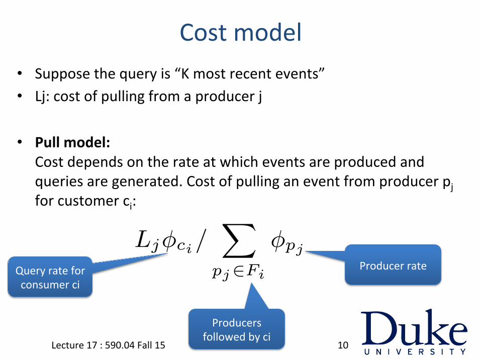
Cost  model  •  Suppose  the  query  is  “K  most  recent  events”  •  Lj:  cost  of  pulling  from  a  producer  j  

•  Pull  model:    Cost  depends  on  the  rate  at  which  events  are  produced  and  queries  are  generated.  Cost  of  pulling  an  event  from  producer  pj  for  customer  ci:    

Lecture  17  :  590.04  Fall  15   10  

Notation Descriptionpj Producerci Consumerfij “Follows:” consumer ci follows producer pj

Fi The set of all producers that consumer ci followsH The cost to push an event to ci’s feedLj The cost to pull events from pj

ej,k The kth event produced by pj

φpjpj ’s event frequency

φcici’s query frequency

kg Events to show in a feed (global coherency)kp Max events to show per producer in a feed

(per-producer coherency)λm Latency achieved in MinCost

λl Target latency of LatencyConstrainedMinCost

σij Decrease in latency by shifting eij from pull to pushϵij Extra cost from shifting eij from pull to push

Table 1: Notation

examine the optimization problems posed by aggregatingproducers.

3.1 Model and AssumptionsRecall the connection network G(V, F ) from Section 2.1.

This graph is a bi-partite graph from producers to con-sumers. When consumer ci performs a query, we must pro-vide a number of events for ci’s feed. We consider both of thecoherency cases introduced in Section 2. In the global case,we supply the most recent kg events across all producersin Fi. In the per-producer case, we supply the most recentkp events for each producer in Fi. Table 1 summarizes thenotation we use in this section.The decisions we make for storing producer events and

materialized consumer feeds determine the cost to push orpull events. We denote H as the cost to push an event toci’s feed, and Lj as the cost to pull a small constant numberof events from producer pj . Lj might vary between produc-ers if we obtain their streams from different systems. Weassume kp and kg are both small enough that Lj will be thesame for each. Note that we assume that multiple eventscan be retrieved using a pull from a single producer. Thisis true if we have stored the events from producer streams,clustered by producer; a single remote procedure call canretrieve multiple events; and the disk cost (if any) for re-trieving events is constant for a small number of events (e.g.since any disk cost is dominated by a disk seek). We do notconsider the cost to ingest and store producer events; thiscost would be the same regardless of strategy.Furthermore, we assume that the H and Lj costs are con-

stant, even as load increases in the system. If the systembottleneck changes with increasing event rate or producerfanout, this assumption may not be true. For example, wemay materialize data in memory, but if the number of con-sumers or producer fan-out changes, the data may grow andspill over to disk. This would change the push and pull coststo include disk access. Usually we can provision enough re-sources (e.g. memory, bandwidth, CPU etc.) to avoid thesebottleneck changes and keep H and Lj constant. Our anal-ysis does not assume data is wholly in memory, but doesassume the costs are constant as the system scales.

3.2 Cost OptimizationWe now demonstrate that the appropriate granularity for

decision making is to decide whether to push or pull indi-vidually for each producer/consumer pair.

3.2.1 Per-Producer CoherencyWe begin with the per-producer coherency case. For ci,

pj and event ej,k, we derive the lifetime cost to deliver ej,kto ci. The lifetime of ej,k is the time from its creation to thetime when pj has produced kp subsequent events.

Claim 1. Assume that we have provisioned the systemwith sufficient resources so that the costs to push and pull anindividual event are constant as the system scales. Further,assume pull cost is amortized over all events acquired withone pull. Then, the push and pull lifetime costs for an eventej,k by pj for ci under per-producer coherency are:

Push cost over ej,k’s lifetime = H

Pull cost over ej,k’s lifetime = Lj(φci/φpj )

Proof: Push cost is oblivious to event lifetime; we pay Honce for the event. Pull cost does depend on lifetime. Eventej,k has lifetime kp/φpj . Over this lifetime, the number oftimes ci sees ej,k is φci(kp/φpj ). The cost to pull ej,k is(Lj/kp) (Lj amortized over each pulled event). Thus, life-time cost for ej,k is (Lj/kp)φci(kp/φpj ) = Lj(φci/φpj ). ✷

Then, we can conclude that for a given event, we shouldpush to a given consumer if the push cost is lower than pull;and pull otherwise. Since the push and pull cost depend onlyon producer and consumer rates, we can actually make onedecision for all the events on a particular producer/consumerpair. We can derive the optimal decision rule:

Lemma 1. Under per-producer coherency, the policy whichminimizes cost for handling events from pj for ci is:

If (φci/φpj ) >= H/Lj , push for all events by pj

If (φci/φpj ) < H/Lj , pull for all events by pj

Proof: The push vs. pull decision draws directly from thecosts in Claim 1. ✷

3.2.2 Global CoherencyUnder global coherency, ci’s feed contains the kg most

recent events across all producers in Fi.

Claim 2. Assume that we have provisioned the systemwith sufficient resources so that the costs to push and pull anindividual event are constant as the system scales. Further,assume pull cost is amortized over all events acquired withone pull. Then, the push and pull lifetime costs for an eventej,k by pj for ci under global coherency are:

Push cost over ej,k’s lifetime = H

Pull cost over ej,k’s lifetime = Ljφci/∑

pj∈Fi

φpj

Proof: The proof for the global case is similar to the per-producer case, with a few key differences. Producer fre-quency is an aggregate over all of Fi: φFi =

∑pj∈Fi

φpj .

Event ej,k has lifetime kg/φFi , and its amortized pull cost isL/kg. We substitute these terms in the per-producer anal-ysis and reach the push and pull costs for global coherency.We omit the complete derivation. ✷

We can then derive the optimal decision rule for a (pro-ducer, consumer) pair in the global coherency case.

Query  rate  for  consumer  ci  

Producers  followed  by  ci  

Producer  rate  

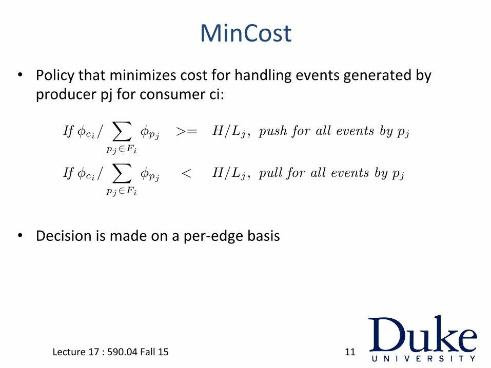
MinCost  •  Policy  that  minimizes  cost  for  handling  events  generated  by  

producer  pj  for  consumer  ci:    

•  Decision  is  made  on  a  per-­‐edge  basis  

Lecture  17  :  590.04  Fall  15   11  

Lemma 2. Under global coherency, the policy which min-imizes cost for handling events from pj for ci is:

If φci/∑

pj∈Fi

φpj >= H/Lj , push for all events by pj

If φci/∑

pj∈Fi

φpj < H/Lj , pull for all events by pj

Proof: The push vs. pull decision draws directly from thecosts in Claim 2. ✷We summarize our main findings from Lemmas 1 and 2.

Under per-producer coherency, the lifetime cost for an eventfor a particular consumer is dependent on both consumerfrequency and the event’s producer frequency. Under globalcoherency, lifetime cost for an event is dependent on bothconsumer frequency and the aggregate event frequency ofthe producers that the consumer follows.

3.2.3 MinCost

We have shown how to minimize cost for individual pro-ducer/consumer edges. We now show that such local deci-sion making is globally optimal.

Theorem 1. For per-producer coherency, the MinCost so-lution is derived by separately choosing push or pull for eachproducer/consumer pair, with push vs. pull per pair deter-mined by Lemma 1.

Proof: We minimize global cost by minimizing the cost paidfor every event. Similarly, we minimize the cost for an eventby minimizing the cost paid for that event for every con-sumer. Lemma 1 assigns each edge push or pull to minimizethe cost paid for events between the edge’s consumer andproducer. Further, no assignment made on any one edgeimposes any restrictions on the assignments we can maketo any other edges. Therefore, minimizing cost for everyconsumer and event minimizes global cost. ✷

Theorem 2. For global coherency, MinCost is derived byseparately choosing push or pull for each consumer, withpush vs. pull per consumer determined by Lemma 2.

Proof: The proof mirrors that of Theorem 1. In this case,Lemma 1 assigns all edges either push or pull. Again,no edge assignment restricts any other edge assignments.Therefore, minimizing cost for every consumer and eventminimizes global cost. ✷Theorems 1 and 2 have important theoretical and prac-

tical implications. The ability to separately optimize eachedge makes minimizing overall cost simple. Moreover, asquery and event rates change over time and new edges areadded, we do not need to re-optimize the entire system. Wesimply optimize changed and new edges, while leaving un-changed edges alone, and find the new MinCost plan.We also observe that any system is subject to different

query and event rates, and skew controlling which consumersor producers contribute most to these rates. To find theMinCost, however, there is no need to extract or understandthese patterns. Instead, we need only separately measureeach consumer’s query rate and compare it to the event rateof the producers that the consumer follows (either individ-ually or in aggregate).

3.3 Optimizing Query LatencyTo this point, our analysis has targeted MinCost. We

now consider LatencyConstrainedMinCost, which respectsan SLA (e.g. 95% of requests execute within 100 ms). Min-Cost may already meet the SLA. If not, we may be able toshift pull edges to push, raising cost, but reducing work atquery time, and meet the SLA. We might also move to apush-only strategy and still not meet a very stringent SLA.In this section we analyze the case where pushing helps, butat a cost. We ultimately provide a practical adaptive algo-rithm that approximates LatencyConstrainedMinCost.

Suppose MinCost produces a latency of λm, while La-tencyConstrainedMinCost requires a latency of λl, whereλl < λm. Intuitively, we can shift edges that are pull inMinCost to push and reduce latency. Formally, we defineσij as the decrease in global latency gained by shifting eijto push. We define ϵij as the penalty from doing this shift.Formally, ϵij = φpj (H − Lj(φci/φpj )) for per-producer co-herency; this is the extra cost paid per event for doing pushinstead of pull, multiplied by pj ’s event rate.

Consider the set of edges pulled in MinCost, R. To findLatencyConstrainedMinCost, our problem is to choose asubset of these edges S to shift to push, such that

∑S σij ≥

(λm − λl) and∑

S ϵij is minimized. Solving for S is equiva-lent to the knapsack problem [19], and is therefore NP-hard.We sketch this equivalence.

Lemma 3. LatencyConstrainedMinCost is equivalent toknapsack.

Proof sketch: We start by reducing knapsack to Laten-cyConstrainedMinCost. Consider the standard knapsackproblem. There exists a weight constraint W and set of nitems I, where the ith item in I has value vi and weightwi. The problem is to find a subset of items K such that∑

i∈K wi ≤ W and∑

i∈K vi is maximized. We can convertthis to an equivalent problem of finding the set of itemsK′ omitted from the knapsack. Assume

∑i∈I wi = T .

The problem is to find K′ such that∑

i∈K′ wi ≥ T − Wand

∑i∈K′ vi is minimized. Through variable substitution

(omitted), we show the omitted knapsack problem is La-tencyConstrainedMinCost. We can similarly reduce Laten-cyConstrainedMinCost to knapsack. This verifies the twoproblems are equivalent. ✷

3.3.1 Adaptive AlgorithmWe are left with two issues. First, knapsack problems are

NP-hard [19]. Second, we have defined σij as the reductionin latency from shifting fij to push; in practice, we find thatwe can not accurately predict the benefit gained by shiftingan edge to push. We now show how we handle both issueswith an adaptive algorithm.

Though we do not know the exact latency reduction fromshifting an edge to push, choosing a higher rate consumershould result in a greater reduction, since this benefits morefeed retrievals. Therefore, we set σij = φci , estimate the∑

φci that does reduce latency by (λm − λl), and solve forS. We measure whether S exactly meets the SLA. If not,we adapt: if latency is too high, we solve for a larger

∑φci :

if latency is too low, we solve for a smaller∑

φci .We want a solution that incurs only incremental cost when

we adjust the target∑

φci . Moreover, the knapsack problemis NP-hard, so our solution must provide a suitable approx-imation of the optimal solution. To address both concerns,

Latency  Constrained  Problem  •  Pull  strategy  may  reduce  cost,  but  increases  query  latency.    

•  If  pL%  of  the  queries  are  required  to  have  low  latency,  then  one  may  need  to  change  some  of  the  edges  from  Pull  to  Push.  

•  Equivalent  to  a  Knapsack  problem.    

Lecture  17  :  590.04  Fall  15   12  

Summary  Push  vs  Pull  

•  If  a  consumer  queries  the  system  more  ojen  than  its  producer  create  updates,  then  use  Push  

•  If  a  producer  creates  updates  more  ojen  than  queries  from  a  consumer,  then  use  Pull  

Lecture  17  :  590.04  Fall  15   13  

OPEN  RESEARCH  PROBLEMS  

Lecture  17  :  590.04  Fall  15   14  

Open  QuesNons  •  View  SelecNon:  

–  which  views  to  materialize    

•  View  Scheduling:  –  when  to  build  views,  when  to  incrementally  maintain  and  when  to  expire  views  

•  View  Placement:  –  OpNmally  place  views  in  a  distributed  semng  

•  Access  control  and  fine  grained  queries  

•  Handling  Changes  in  the  ConnecNons  graphs  

Lecture  17  :  590.04  Fall  15   15  

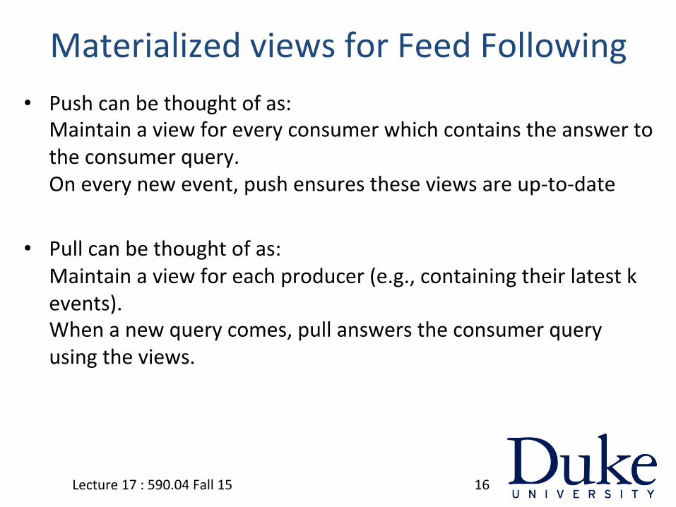
Materialized  views  for  Feed  Following  •  Push  can  be  thought  of  as:  

Maintain  a  view  for  every  consumer  which  contains  the  answer  to  the  consumer  query.  On  every  new  event,  push  ensures  these  views  are  up-­‐to-­‐date  

•  Pull  can  be  thought  of  as:    Maintain  a  view  for  each  producer  (e.g.,  containing  their  latest  k  events).  When  a  new  query  comes,  pull  answers  the  consumer  query  using  the  views.    

Lecture  17  :  590.04  Fall  15   16  

View  SelecNon  Which  type  of  views  should  be  materialized?    OpNmizaNon  Criterion:  •  Update:  Cost  of  maintaining  views  when  a  new  event  enters  the  

system  •  Query:  Cost  of  generaNng  a  user  feed  from  views  •  Memory  footprint:  Total  size  of  all  views  

Lecture  17  :  590.04  Fall  15   17  

View  SelecNon  

Query:  Return  latest  k  events  produced  by  friends.  Design  1:  One  view  per  consumer  (with  latest  k  events  from  friends)  

     

   

   

   

carl  

doris  

eric  

frances  

   george  

   

   

   

   

carl  

doris  

eric  

frances  

   george  

producers   consumers  

Lecture  17  :  590.04  Fall  15   18  

View  SelecNon  Query:  Return  latest  k  events  produced  by  friends.  Design  1:  One  view  per  consumer  (with  latest  k  events  from  friends)  

 Update:  O(degree(producer))  Query:    O(1)  Memory  footprint:  O(#  consumers)  

Lecture  17  :  590.04  Fall  15   19  

View  SelecNon  

Query:  Return  latest  k  events  produced  by  friends.  Design  2:  One  view  per  producer(with  latest  k  events  from  producer)  

     

   

   

   

carl  

doris  

eric  

frances  

   george  

   

   

   

   

carl  

doris  

eric  

frances  

   george  

producers   consumers  

Lecture  17  :  590.04  Fall  15   20  

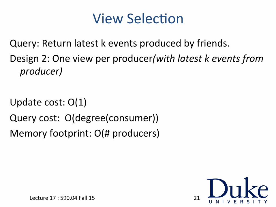
View  SelecNon  Query:  Return  latest  k  events  produced  by  friends.  Design  2:  One  view  per  producer(with  latest  k  events  from  producer)  

 Update  cost:  O(1)  Query  cost:    O(degree(consumer))  Memory  footprint:  O(#  producers)  

Lecture  17  :  590.04  Fall  15   21  

View  SelecNon  

Query:  Return  latest  k  events  produced  by  friends.  Design  3:  One  view  per  set  of  producers  S  (with  latest  k  events  from  producer  in  S)  

     

   

   

   

carl  

doris  

eric  

frances  

   george  

   

   

   

   

carl  

doris  

eric  

frances  

   george  

producers   consumers  

Lecture  17  :  590.04  Fall  15   22  

View  SelecNon  

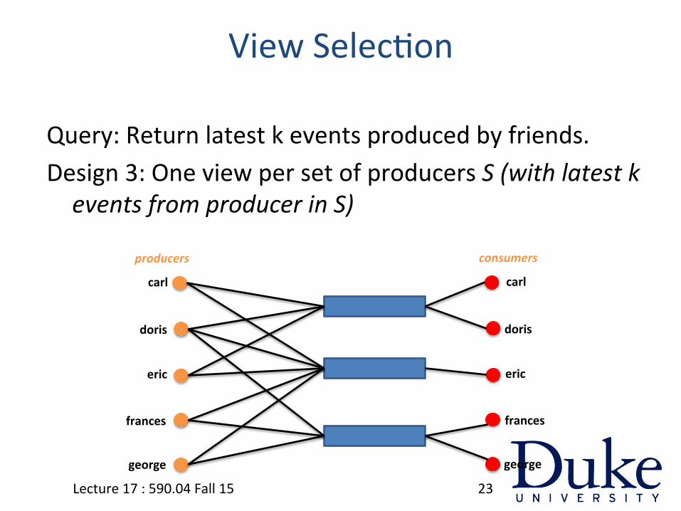
Query:  Return  latest  k  events  produced  by  friends.  Design  3:  One  view  per  set  of  producers  S  (with  latest  k  events  from  producer  in  S)  

     

   

   

   

carl  

doris  

eric  

frances  

   george  

   

   

   

   

carl  

doris  

eric  

frances  

   george  

producers   consumers  

Lecture  17  :  590.04  Fall  15   23  

View  SelecNon  

Query:  Return  latest  k  events  produced  by  friends.  Design  3:  One  view  per  set  of  producers  S  (with  latest  k  events  from  producer  in  S)  

     

   

   

   

carl  

doris  

eric  

frances  

   george  

   

   

   

   

carl  

doris  

eric  

frances  

   george  

producers   consumers  

Lecture  17  :  590.04  Fall  15   24  

View  SelecNon  

•  Subset  of  Twi_er  social  graph  

•  400,000  consumers  •  79,842  producers  

•  Design  3:  70,926  views  –  5.6x  improvement  over  

consumer  views  –  12%  improvement  over  

producer  views  

   

0  

100  

200  

300  

400  

Consumer   Producer   Design  3  

Num

ber  o

f  Views  (x  1000)    

Memory  Footprint  

Lecture  17  :  590.04  Fall  15   Skip>>>   25  

View  Scheduling  We  do  not  need  all  views  at  all  Nmes.    When  do  we  evict  them/let  

them  grow  stale  and  when  do  we  rebuild/refresh  them?      •  May  be  able  to  predict  when  users  will  pose  queries.    

•  In  certain  cases,  there  is  a  fixed  schedule  for  queries  –  Regression  tasks  on  a  codebase  are  always  run  at  the  same  Nme  everyday.    

Lecture  17  :  590.04  Fall  15   26  

Signature  Scheduling  

Feasibility  of  view  scheduling:    users  typically  have  a  diurnal  access  pa_ern    

 •  Based  on  access  logs  generate  access  signature          

Lecture  17  :  590.04  Fall  15   27  

Signature  Scheduling  

Hit  Rate:  percentage  of  queries  answered  with  fresh  results    Schedule  Refresh  Threshold:  number  of  queries  a  consumer  must  make  in  training  to  get  signature  refreshes    

Lecture  17  :  590.04  Fall  15   28  

View  Placement  How  to  opNmally  place  views  in  a  distributed  semng?    OpNmizaNon  criteria:  Update:  Number  of  machines  to  be  accessed  to  update  views  on  a  

new  event  Query:  Number  of  machines  to  be  accessed  to  answer  a  user  query  Size  of  each  machine    

Lecture  17  :  590.04  Fall  15   29  

View  Placement  Suppose  consumer  views  must  be  distributed  on  2  machines,  at  

most  3  views  per  machine  

   

   

   

   

carl  

doris  

eric  

frances  

   george  

   

   

   

   

carl  

doris  

eric  

frances  

   george  

producers   consumers  

Lecture  17  :  590.04  Fall  15   30  

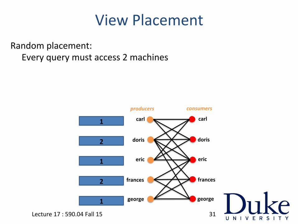
View  Placement  Random  placement:    

Every  query  must  access  2  machines  

   

   

   

   

carl  

doris  

eric  

frances  

   george  

   

   

   

   

carl  

doris  

eric  

frances  

   george  

producers   consumers  

1  

2  

1  

2  

1  

Lecture  17  :  590.04  Fall  15   31  

View  Placement  Intelligent  placement:    

Carl  and  Doris  only  need  to  access  one  machine.    

   

   

   

   

carl  

doris  

eric  

frances  

   george  

   

   

   

   

carl  

doris  

eric  

frances  

   george  

producers   consumers  

1  

1  

1  

2  

2  

Lecture  17  :  590.04  Fall  15   32  

Open  QuesNons  •  View  SelecNon  •  View  Scheduling  •  View  Placement  

•  Access  control  and  fine  grained  queries  

•  Handling  Changes  in  the  ConnecNons  graph  

•  Answering  more  complex  aggregate  queries  over  recent  events  

Lecture  17  :  590.04  Fall  15   33