feedback control of linear siso systems - … · 3 closed-loop system in study and design of...
TRANSCRIPT
1
Feedback Control ofLinear SISO systems
Process Dynamics and ControlProcess Dynamics and Control
2
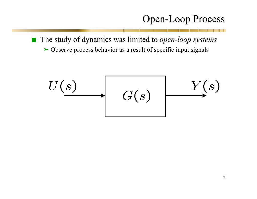
Open-Loop ProcessOpen-Loop Process
The study of dynamics was limited to The study of dynamics was limited to open-loop systemsopen-loop systemsObserve process behavior as a result of specific input signals
3
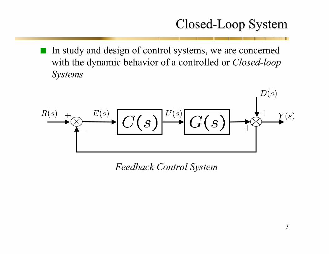
Closed-Loop SystemClosed-Loop System
In study and design of control systems, we are concernedwith the dynamic behavior of a controlled or Closed-loopSystems
Feedback Control System
4
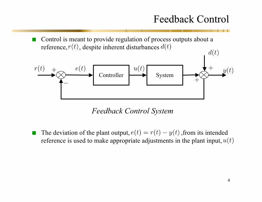
Feedback ControlFeedback Control
Control is meant to provide regulation of process outputs about areference, , despite inherent disturbances
The deviation of the plant output, ,from its intendedreference is used to make appropriate adjustments in the plant input,
Feedback Control System
SystemController
5
Feedback ControlFeedback Control
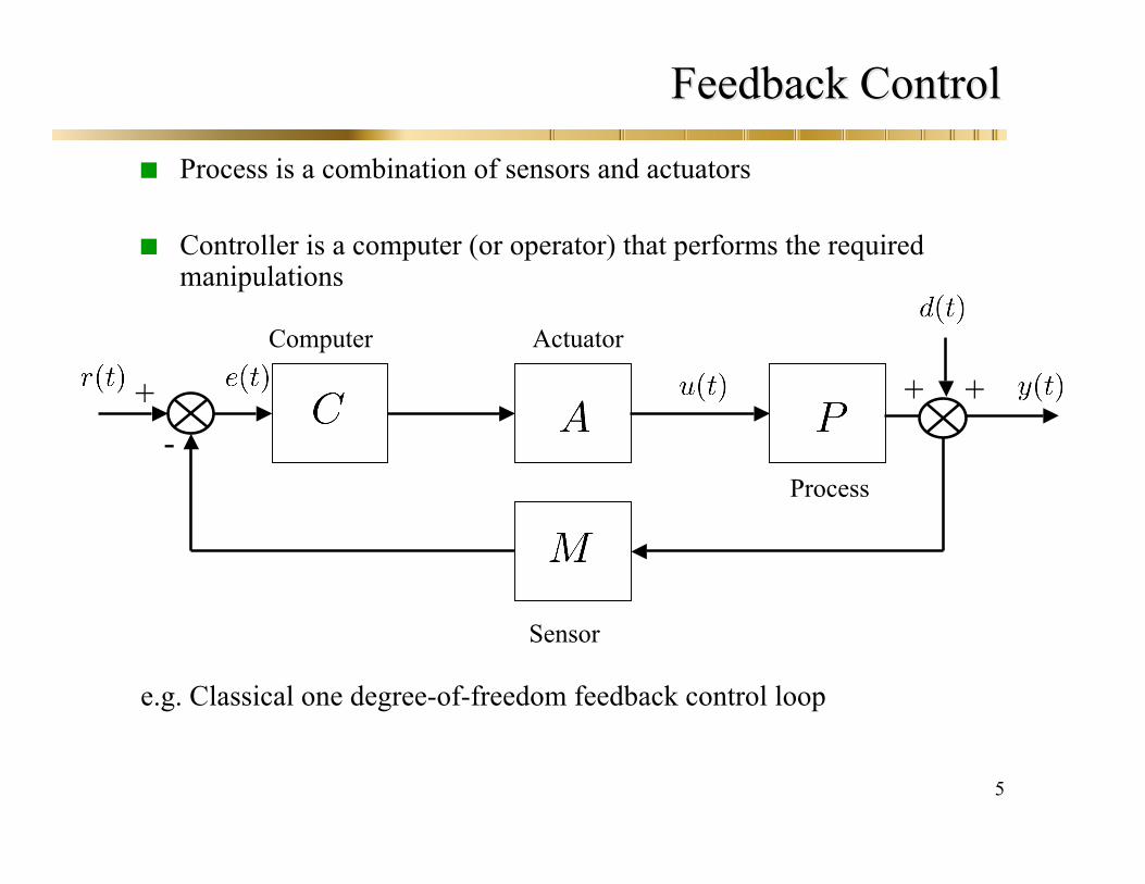
Process is a combination of sensors and actuators
Controller is a computer (or operator) that performs the requiredmanipulations
e.g. Classical one degree-of-freedom feedback control loop
Computer Actuator
Process
Sensor
-+++
6
Closed-Loop Transfer FunctionClosed-Loop Transfer Function
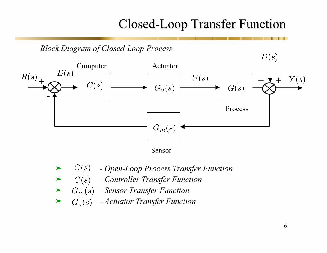
Block Diagram of Closed-Loop Process
- Open-Loop Process Transfer Function - Controller Transfer Function - Sensor Transfer Function - Actuator Transfer Function
Computer Actuator
Process
Sensor
-+++
7
Closed-Loop Transfer FunctionClosed-Loop Transfer Function
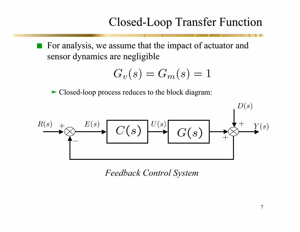
For analysis, we assume that the impact of actuator andFor analysis, we assume that the impact of actuator andsensor dynamics are negligiblesensor dynamics are negligible
Closed-loop process reduces to the block diagram:Closed-loop process reduces to the block diagram:
Feedback Control System
8
Closed-loop Transfer FunctionsClosed-loop Transfer Functions
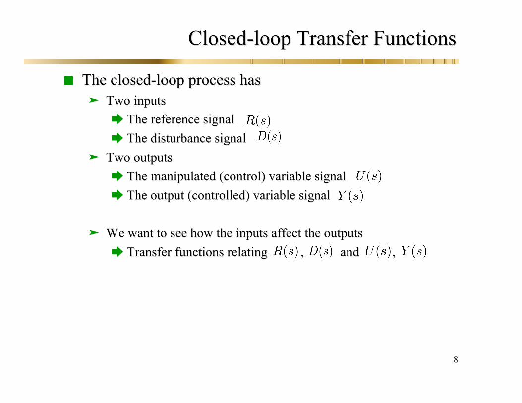
The closed-loop process hasThe closed-loop process has Two inputsTwo inputs
The reference signalThe reference signal The disturbance signal The disturbance signal
Two outputsTwo outputs The manipulatedThe manipulated (control) variable signal(control) variable signal The The output (controlled) variable signaloutput (controlled) variable signal
We want to see how the inputs affect the outputsWe want to see how the inputs affect the outputs Transfer functions relatingTransfer functions relating ,, and , and ,
9
Closed-loop Transfer functionClosed-loop Transfer function
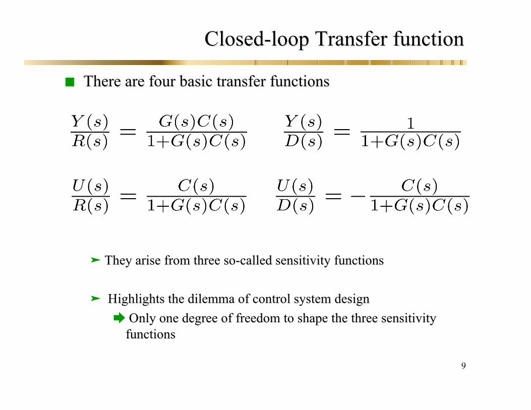
There are four basic transfer functionsThere are four basic transfer functions
They arise from three so-called sensitivity functionsThey arise from three so-called sensitivity functions
Highlights the dilemma of control system designHighlights the dilemma of control system design Only one degree of freedom to shapeOnly one degree of freedom to shape the three sensitivitythe three sensitivity
functionsfunctions
10
Closed-loop Transfer FunctionsClosed-loop Transfer Functions
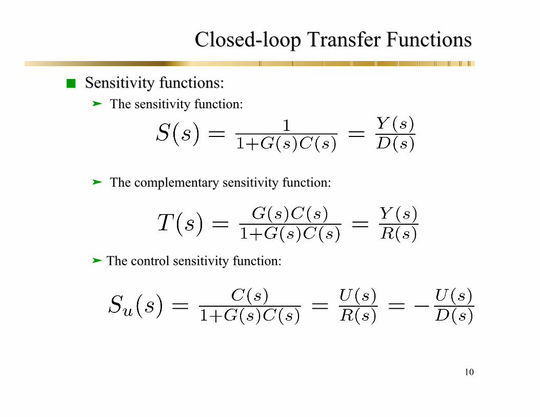
Sensitivity functions:Sensitivity functions: The sensitivity function:The sensitivity function:
The complementary sensitivity function: The complementary sensitivity function:
The control sensitivity function:The control sensitivity function:
11
Closed-loop Transfer FunctionsClosed-loop Transfer Functions
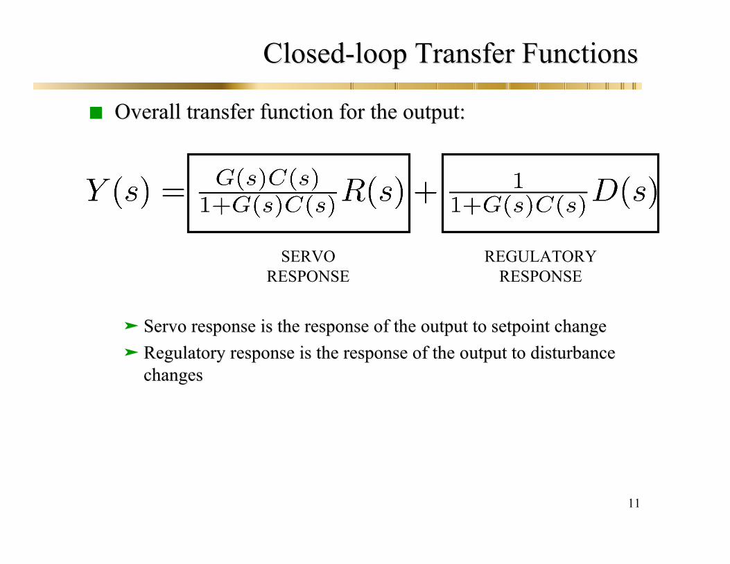
Overall transfer function for the output:Overall transfer function for the output:
Servo response is the response of the output to Servo response is the response of the output to setpoint setpoint changechange Regulatory response is the response of theRegulatory response is the response of the output to disturbanceoutput to disturbance
changeschanges
REGULATORYRESPONSE
SERVORESPONSE
12
Closed-loop Transfer FunctionsClosed-loop Transfer Functions
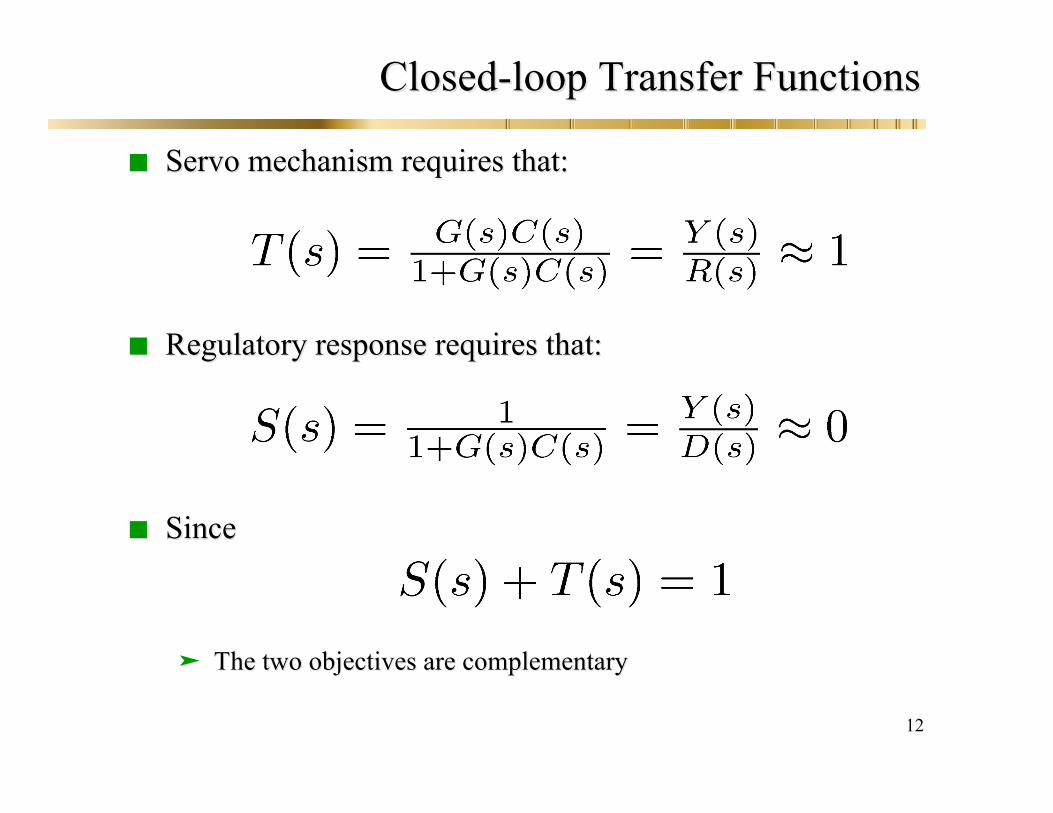
Servo mechanism requires that:Servo mechanism requires that:
Regulatory response requires that:Regulatory response requires that:
SinceSince
The two objectives are complementaryThe two objectives are complementary
13
Closed-loop Transfer FunctionsClosed-loop Transfer Functions
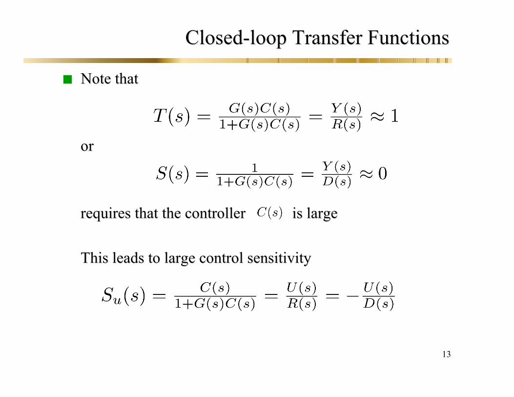
Note thatNote that
oror
requires that the controllerrequires that the controller is largeis large
This leads to large control sensitivityThis leads to large control sensitivity

14
PID ControllerPID Controller
Most widespread choice for the controller is the PID controller
The acronym PID stands for:P - ProportionalI - IntegralD - Derivative
PID Controllers:greater than 90% of all control implementationsdates back to the 1930svery well studied and understoodoptimal structure for first and second order processes (given
some assumptions)always first choice when designing a control system
15
PID ControlPID Control
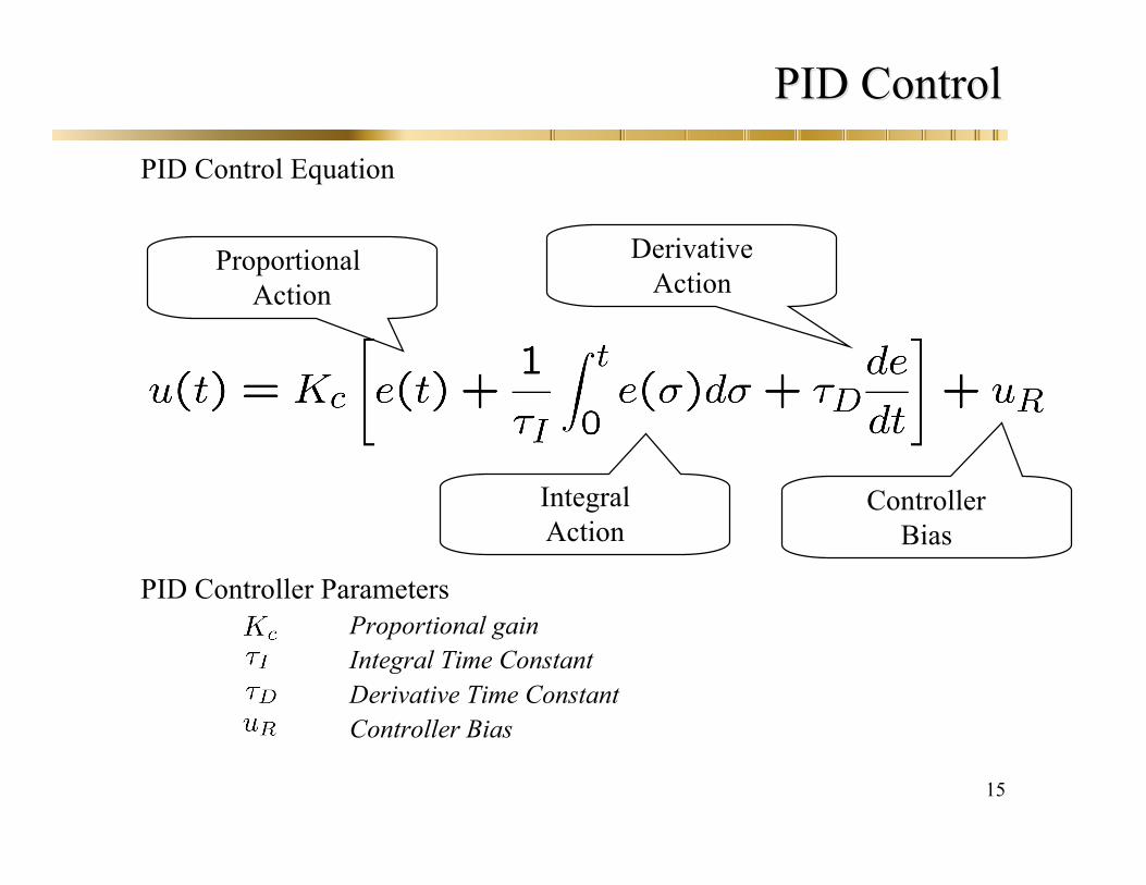
PID Control Equation
PID Controller ParametersKc Proportional gain
Integral Time ConstantDerivative Time ConstantController Bias
Proportional Action
IntegralAction
DerivativeAction
ControllerBias
16
PID ControlPID Control
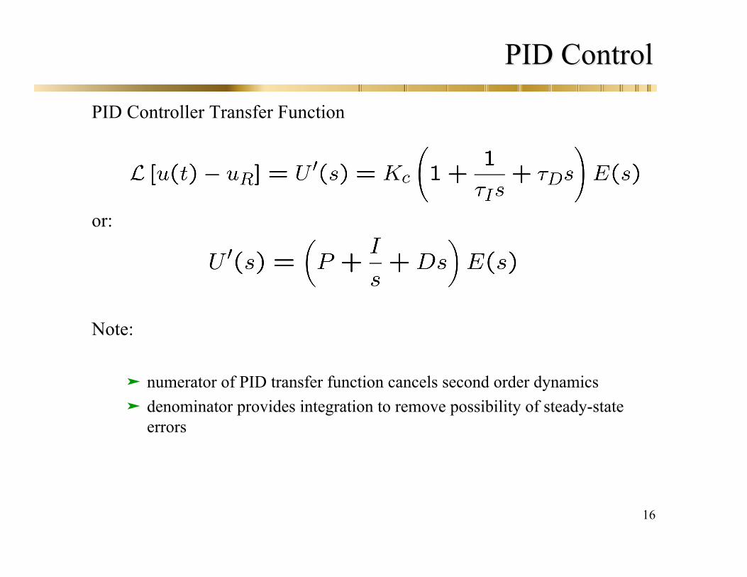
PID Controller Transfer Function
or:
Note:
numerator of PID transfer function cancels second order dynamics denominator provides integration to remove possibility of steady-state
errors
17
PID ControlPID Control
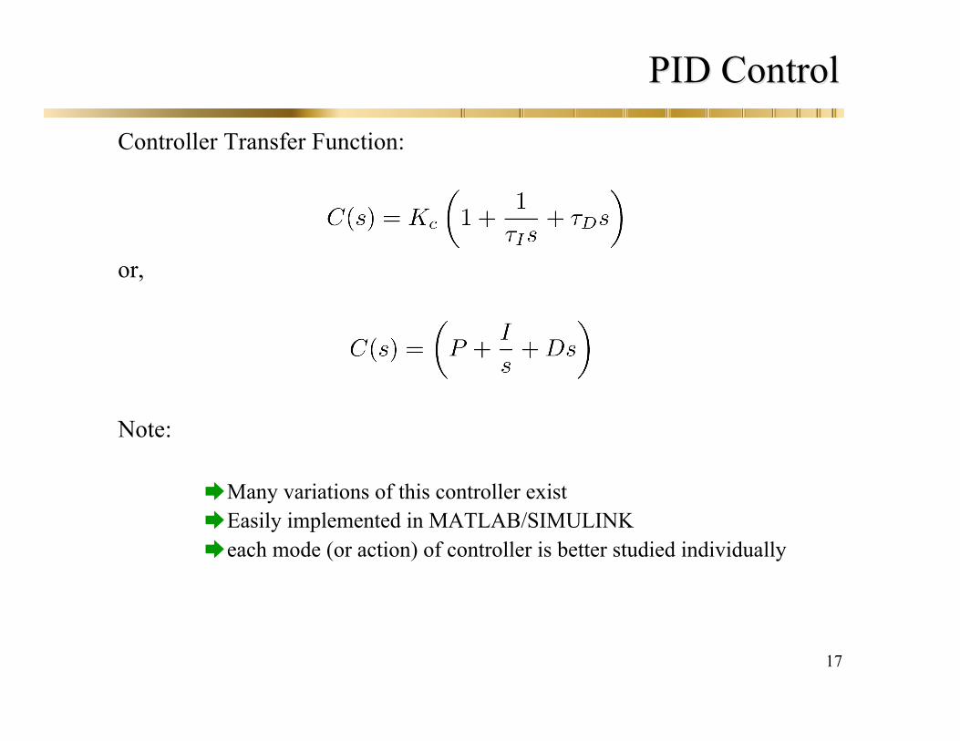
Controller Transfer Function:
or,
Note:
Many variations of this controller existEasily implemented in MATLAB/SIMULINKeach mode (or action) of controller is better studied individually
18
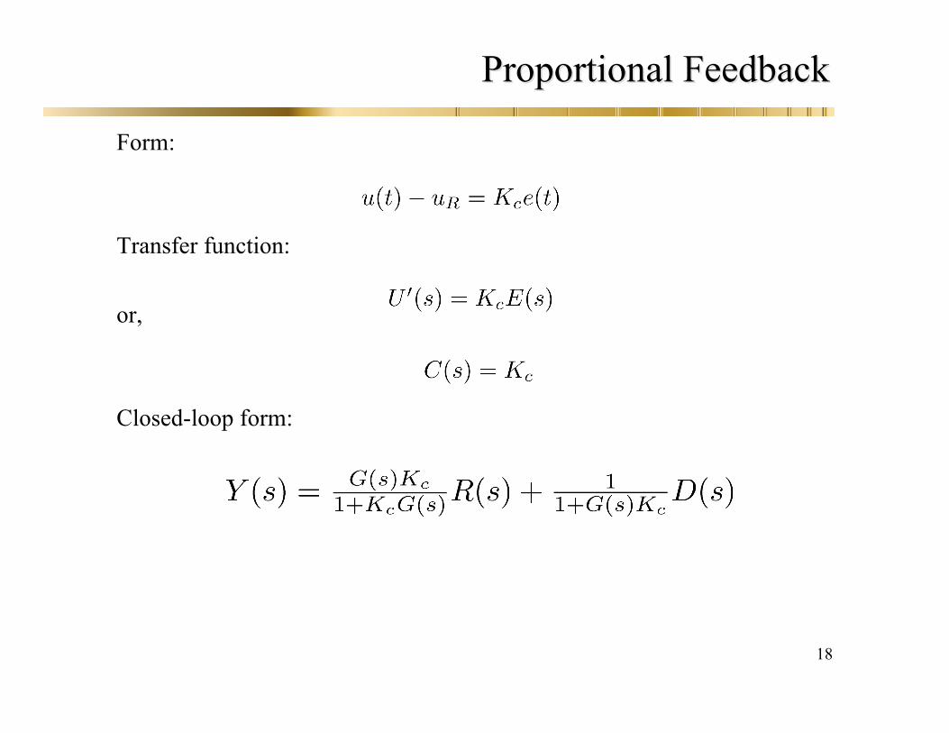
Proportional FeedbackProportional Feedback
Form:
Transfer function:
or,
Closed-loop form:
19
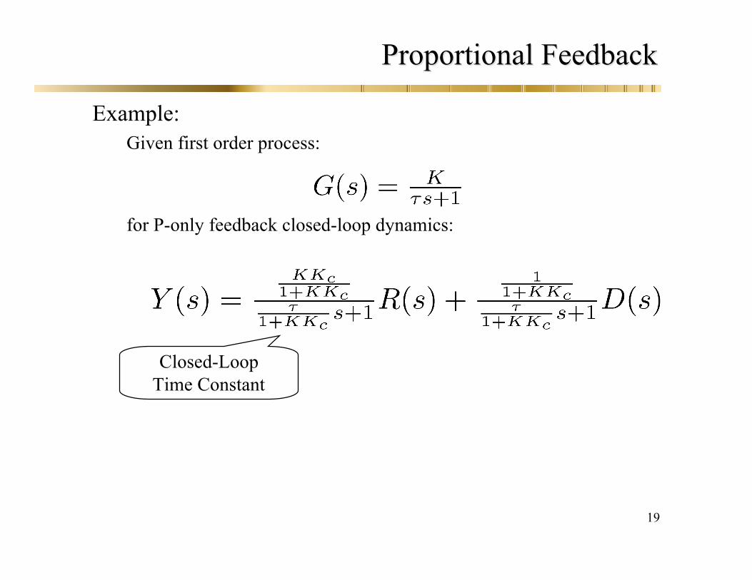
Proportional FeedbackProportional Feedback
Example:Given first order process:
for P-only feedback closed-loop dynamics:
Closed-LoopTime Constant

20
Proportional FeedbackProportional Feedback
Final response:
Note: for “zero offset response” we require
Possible to eliminate offset with P-only feedback (requires infinitecontroller gain)
Need different control action to eliminate offset (integral)
Tracking Error Disturbance rejection
21
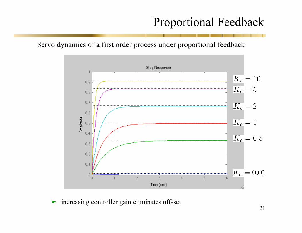
Proportional Feedback
Servo dynamics of a first order process under proportional feedback
increasing controller gain eliminates off-set
22
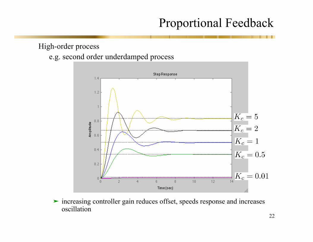
Proportional Feedback
High-order processe.g. second order underdamped process
increasing controller gain reduces offset, speeds response and increasesoscillation
23
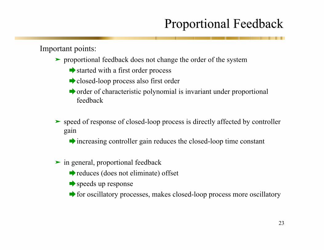
Proportional FeedbackProportional Feedback
Important points: proportional feedback does not change the order of the system
started with a first order processclosed-loop process also first orderorder of characteristic polynomial is invariant under proportional
feedback
speed of response of closed-loop process is directly affected by controllergain increasing controller gain reduces the closed-loop time constant
in general, proportional feedback reduces (does not eliminate) offset speeds up response for oscillatory processes, makes closed-loop process more oscillatory
24
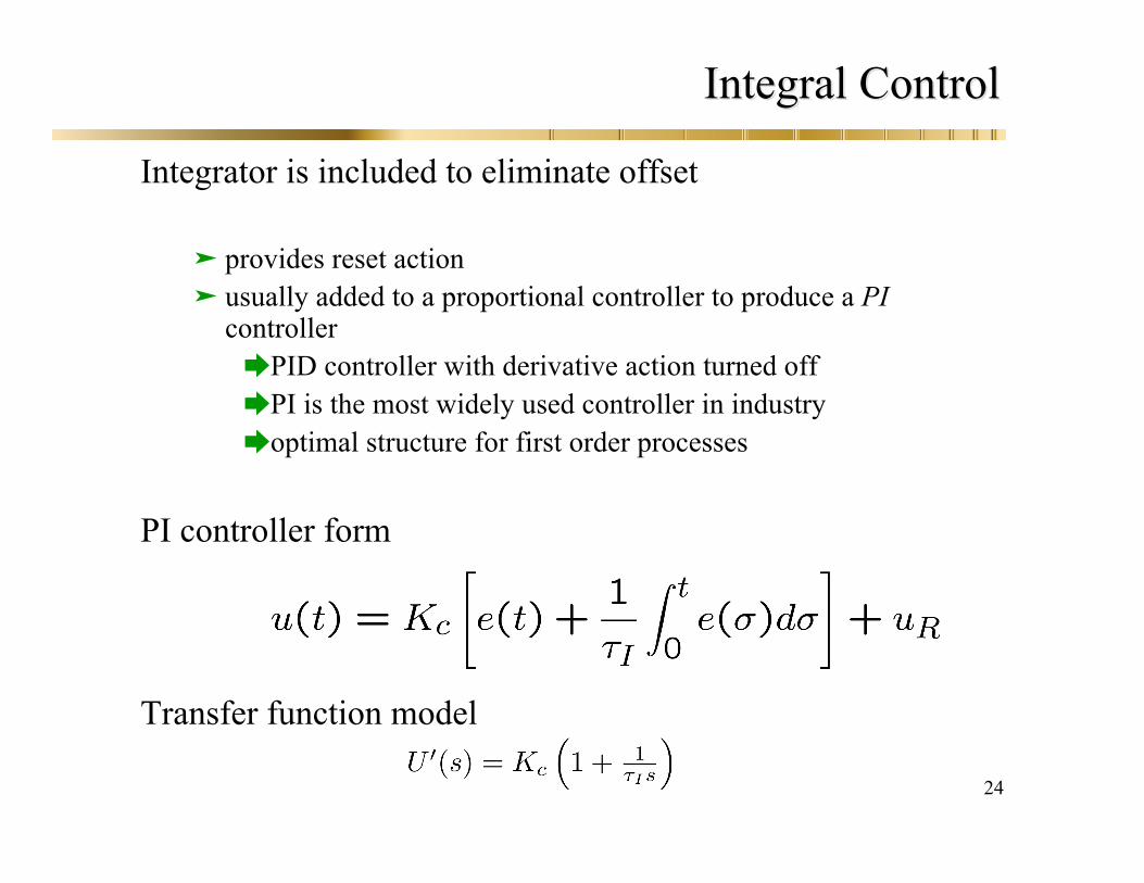
Integral ControlIntegral Control
Integrator is included to eliminate offset
provides reset action usually added to a proportional controller to produce a PI
controllerPID controller with derivative action turned offPI is the most widely used controller in industryoptimal structure for first order processes
PI controller form
Transfer function model
25
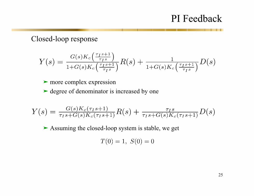
PI FeedbackPI Feedback
Closed-loop response
more complex expression degree of denominator is increased by one
Assuming the closed-loop system is stable, we get
26
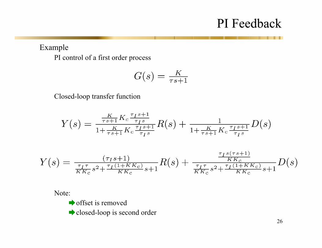
PI FeedbackPI Feedback
ExamplePI control of a first order process
Closed-loop transfer function
Note:offset is removedclosed-loop is second order
27
PI FeedbackPI Feedback
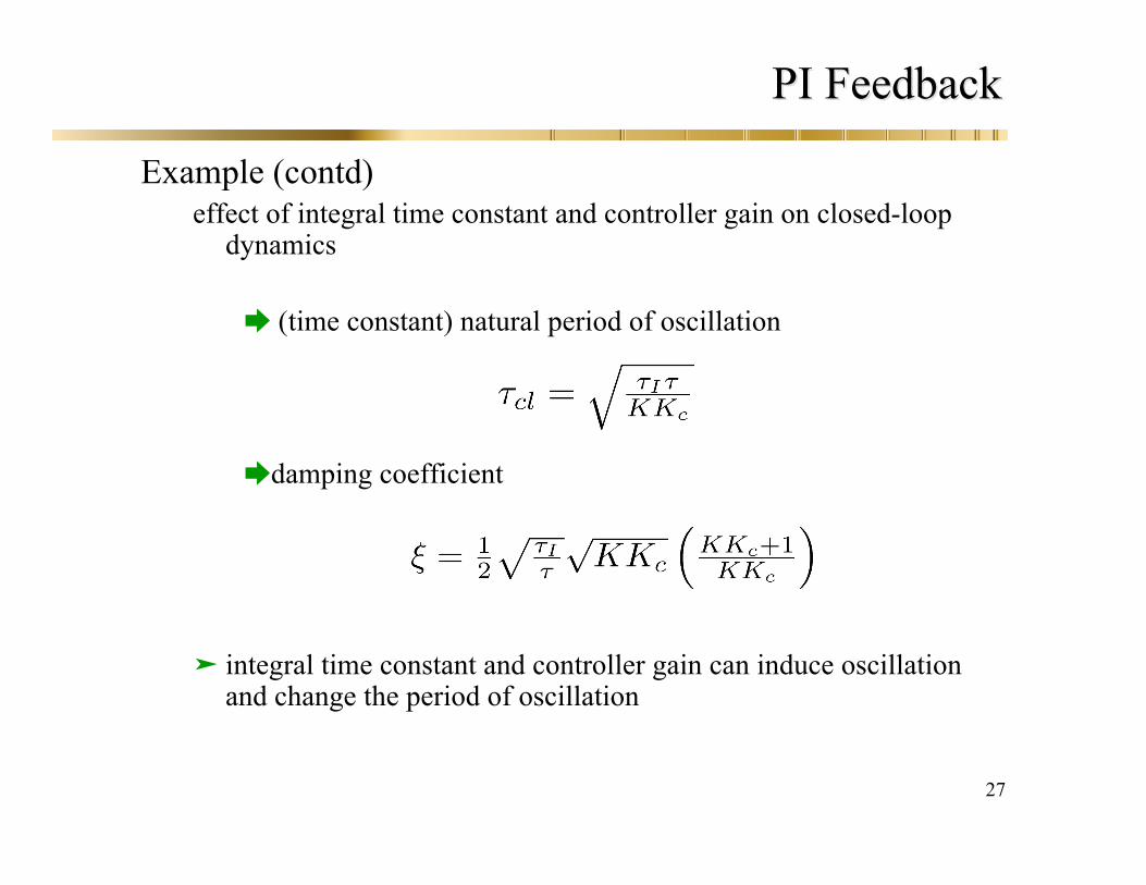
Example (contd)effect of integral time constant and controller gain on closed-loop
dynamics
(time constant) natural period of oscillation
damping coefficient
integral time constant and controller gain can induce oscillationand change the period of oscillation
28
PI Feedback
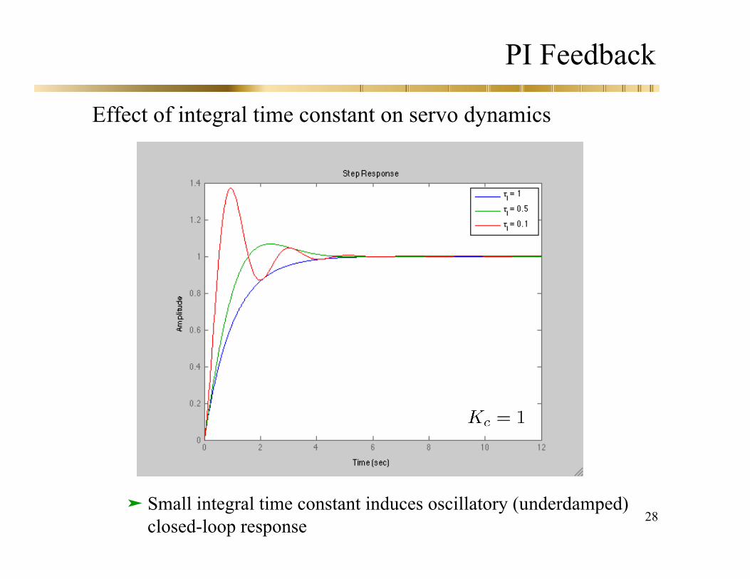
Effect of integral time constant on servo dynamics
Small integral time constant induces oscillatory (underdamped)closed-loop response
29
PI Feedback
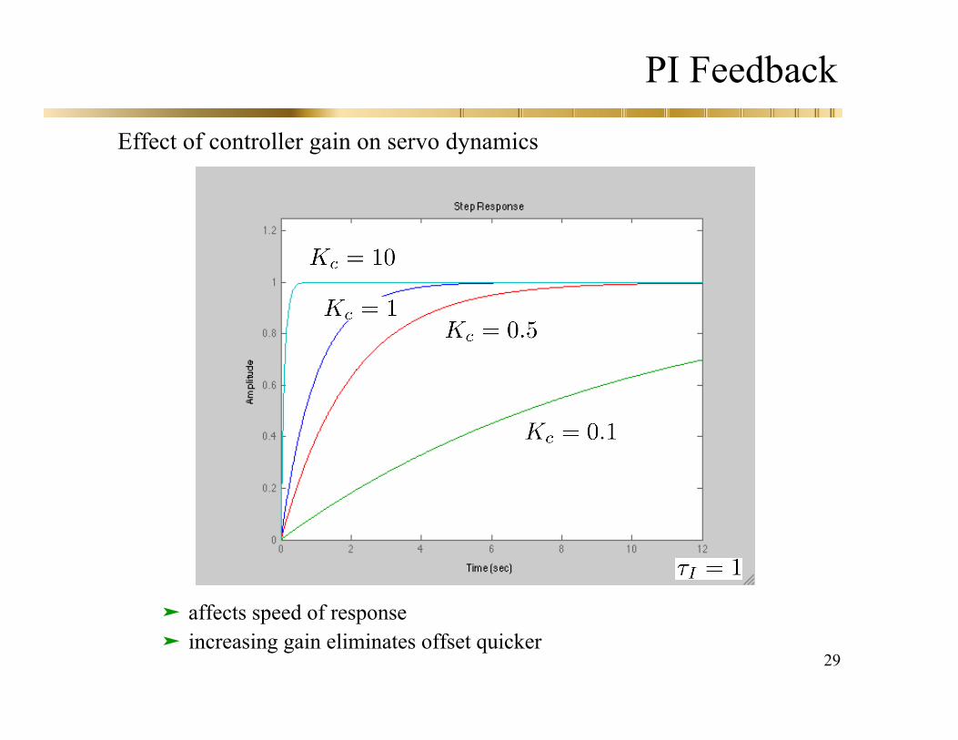
Effect of controller gain on servo dynamics
affects speed of response increasing gain eliminates offset quicker
30
PI Feedback
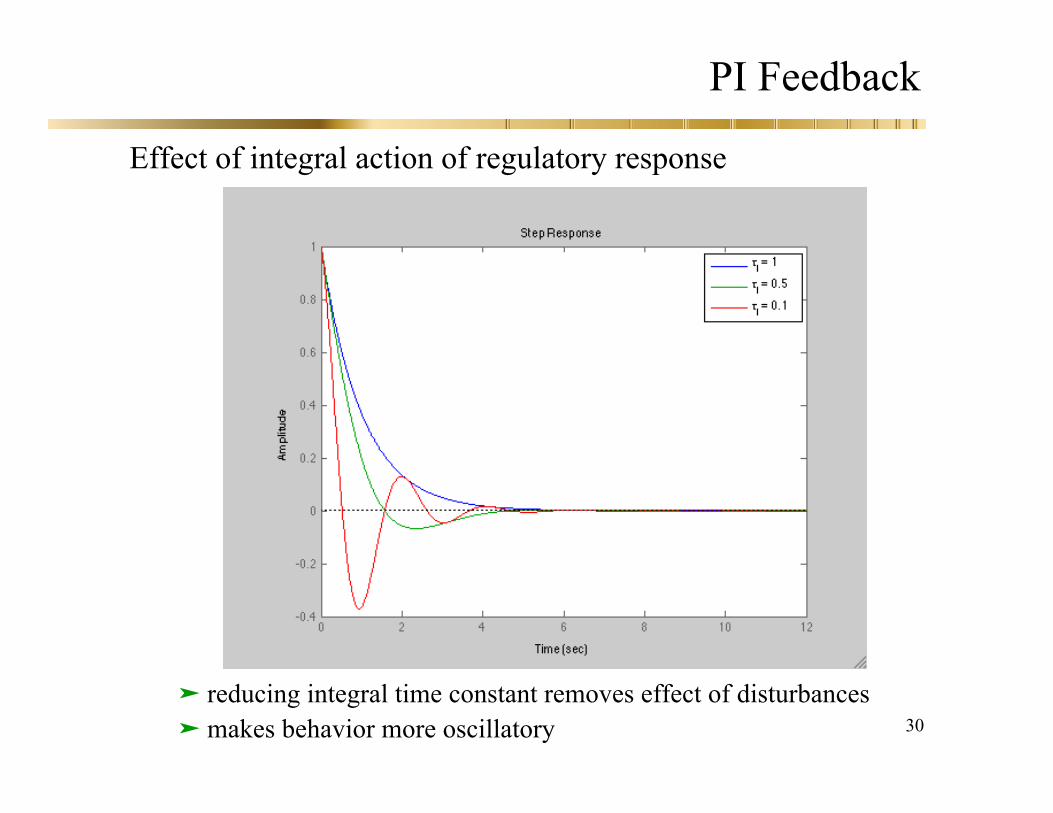
Effect of integral action of regulatory response
reducing integral time constant removes effect of disturbancesmakes behavior more oscillatory
31
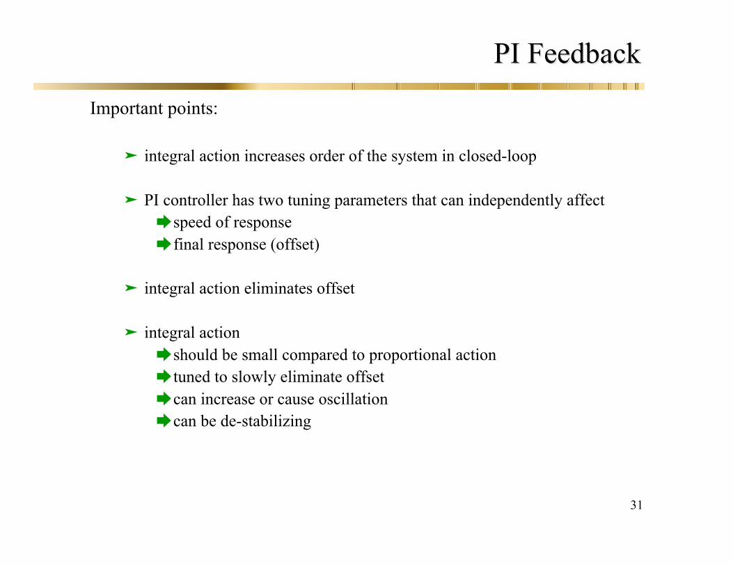
PI FeedbackPI Feedback
Important points:
integral action increases order of the system in closed-loop
PI controller has two tuning parameters that can independently affect speed of response final response (offset)
integral action eliminates offset
integral action should be small compared to proportional action tuned to slowly eliminate offsetcan increase or cause oscillationcan be de-stabilizing
32
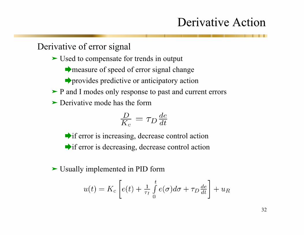
Derivative ActionDerivative Action
Derivative of error signalUsed to compensate for trends in output
measure of speed of error signal changeprovides predictive or anticipatory action
P and I modes only response to past and current errorsDerivative mode has the form
if error is increasing, decrease control actionif error is decreasing, decrease control action
Usually implemented in PID form
33
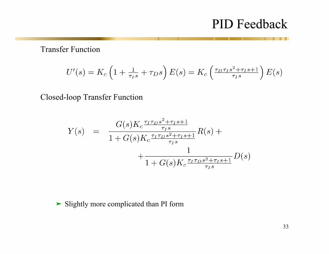
PID FeedbackPID Feedback
Transfer Function
Closed-loop Transfer Function
Slightly more complicated than PI form
34
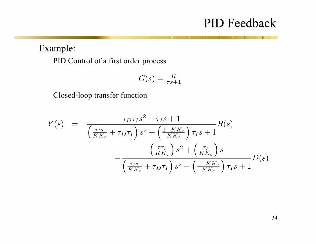
PID FeedbackPID Feedback
Example:PID Control of a first order process
Closed-loop transfer function

35
PID Feedback
Effect of derivative action on servo dynamics
Increasing derivative action leads to a more sluggish servo responseIncreasing derivative action leads to a more sluggish servo response
36
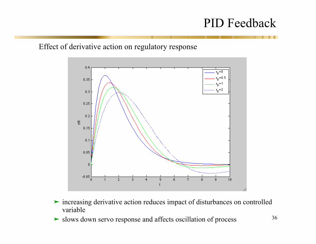
PID Feedback
Effect of derivative action on regulatory response
increasing derivative action reduces impact of disturbances on controlledvariable
slows down servo response and affects oscillation of process
37
PD FeedbackPD Feedback
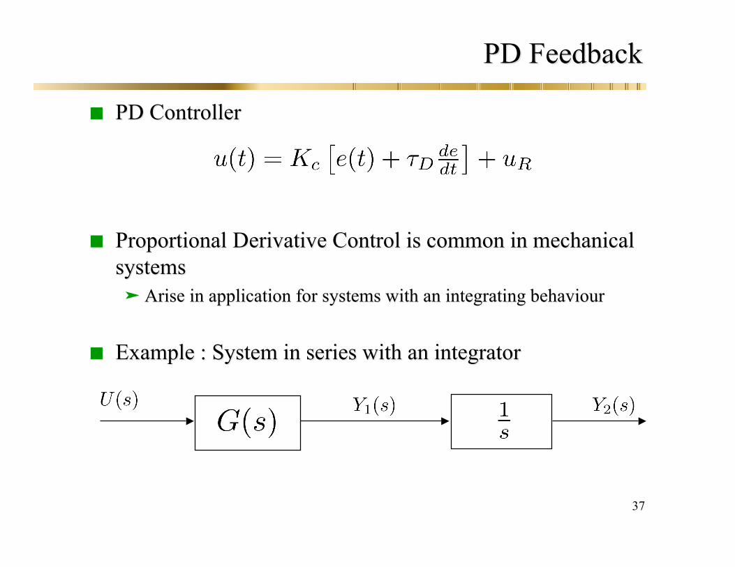
PD ControllerPD Controller
ProportionalProportional Derivative Control is common in mechanicalDerivative Control is common in mechanicalsystemssystems Arise in application for systems with an integratingArise in application for systems with an integrating behaviourbehaviour
Example : System in series with an integratorExample : System in series with an integrator
38
PD FeedbackPD Feedback
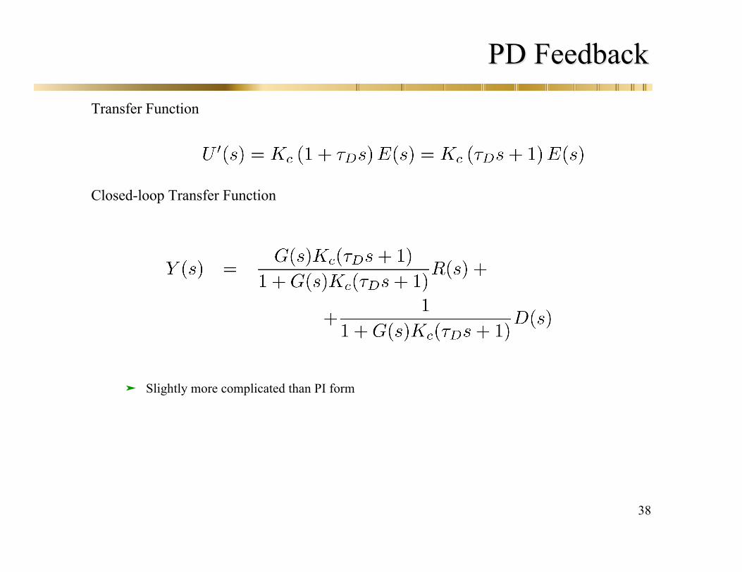
Transfer Function
Closed-loop Transfer Function
Slightly more complicated than PI form
39
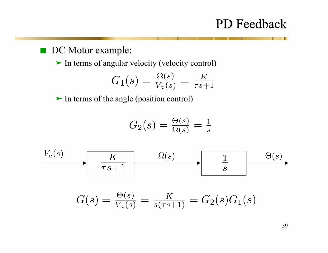
PD FeedbackPD Feedback
DCDC Motor example:Motor example: In terms of angular velocityIn terms of angular velocity (velocity control)(velocity control)
In terms of the angle (position control)In terms of the angle (position control)
40
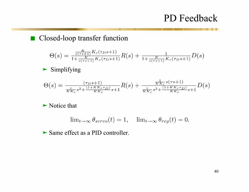
PD FeedbackPD Feedback
Closed-loop transfer functionClosed-loop transfer function
SimplifyingSimplifying
Notice thatNotice that
Same effect as a PID controller.Same effect as a PID controller.
41
Derivative ActionDerivative Action
Important Points:
Characteristic polynomial is similar to PI derivative action does not increase the order of the system adding derivative action affects the period of oscillation of the process
good for disturbance rejectionpoor for tracking
the PID controller has three tuning parameters and can independentlyaffect, speed of response final response (offset) servo and regulatory response
derivative action should be small compared to integral actionhas a stabilizing influencedifficult to use for noisy signalsusually modified in practical implementation
42
Closed-loop Stability
Every control problem involves a consideration of closed-loop stability
General concepts:
Bounded Input Bounded Output (BIBO) Stability:
An (unconstrained) linear system is said to be stable if the outputresponse is bounded for all bounded inputs. Otherwise it is unstable.
Comments:Stability is much easier to prove than instabilityThis is just one type of stability
43
Closed-loop Stability
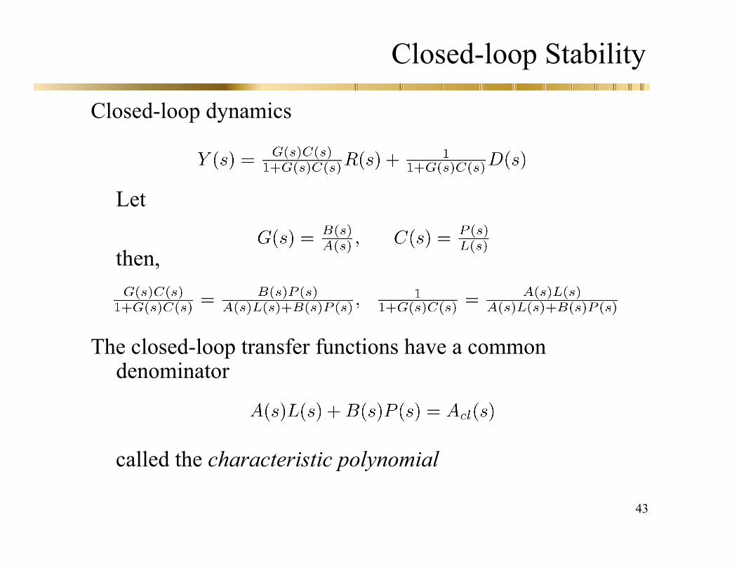
Closed-loop dynamics
Let
then,
The closed-loop transfer functions have a commondenominator
called the characteristic polynomial
44
Closed-loop stability
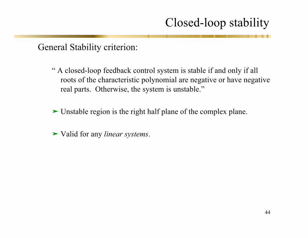
General Stability criterion:
“ A closed-loop feedback control system is stable if and only if allroots of the characteristic polynomial are negative or have negativereal parts. Otherwise, the system is unstable.”
Unstable region is the right half plane of the complex plane.
Valid for any linear systems.
45
Closed-loop Stability
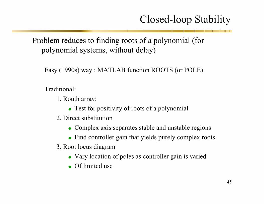
Problem reduces to finding roots of a polynomial (forpolynomial systems, without delay)
Easy (1990s) way : MATLAB function ROOTS (or POLE)
Traditional:1. Routh array:
Test for positivity of roots of a polynomial2. Direct substitution
Complex axis separates stable and unstable regions Find controller gain that yields purely complex roots
3. Root locus diagram Vary location of poles as controller gain is varied Of limited use
46
Closed-loop stability
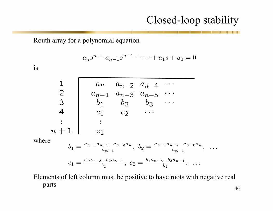
Routh array for a polynomial equation
is
where
Elements of left column must be positive to have roots with negative realparts
47
Example: Routh Array
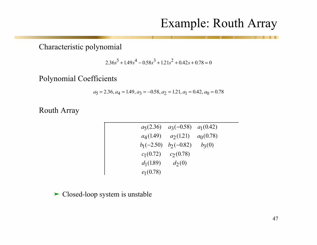
Characteristic polynomial
Polynomial Coefficients
Routh Array
Closed-loop system is unstable
2 36 149 058 121 0 42 0 78 05 4 3 2. . . . . .s s s s s+ ! + + + =
a a aa a ab b bc cd de
5 3 1
4 2 0
1 2 3
1 2
1 2
1
2 36 058 0 42149 121 0 782 50 082 00 72 0 78189 00 78
( . ) ( . ) ( . )( . ) ( . ) ( . )( . ) ( . ) ( )( . ) ( . )( . ) ( )( . )
!
! !
a a a a a a5 4 3 2 1 02 36 149 058 121 0 42 0 78= = = ! = = =. , . , . , . , . , .
48
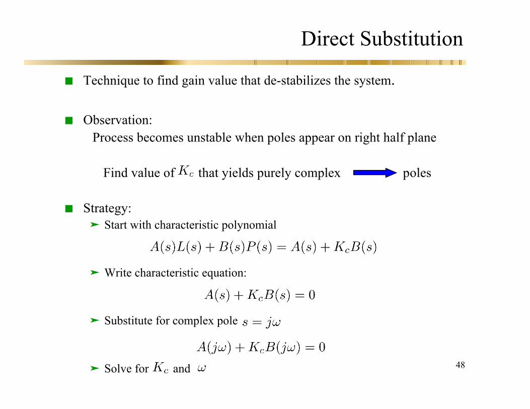
Direct Substitution
Technique to find gain value that de-stabilizes the system.
Observation: Process becomes unstable when poles appear on right half plane
Find value of that yields purely complex poles
Strategy: Start with characteristic polynomial
Write characteristic equation:
Substitute for complex pole
Solve for and
49
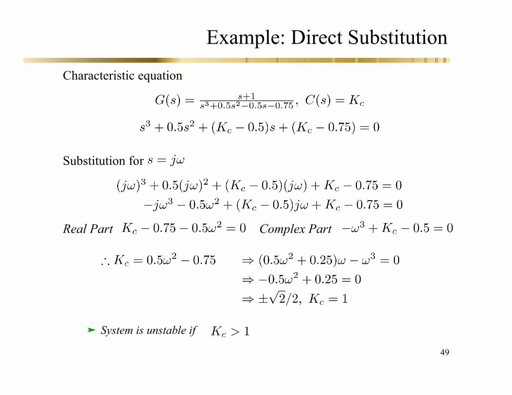
Example: Direct Substitution
Characteristic equation
Substitution for
Real Part Complex Part
System is unstable if
50
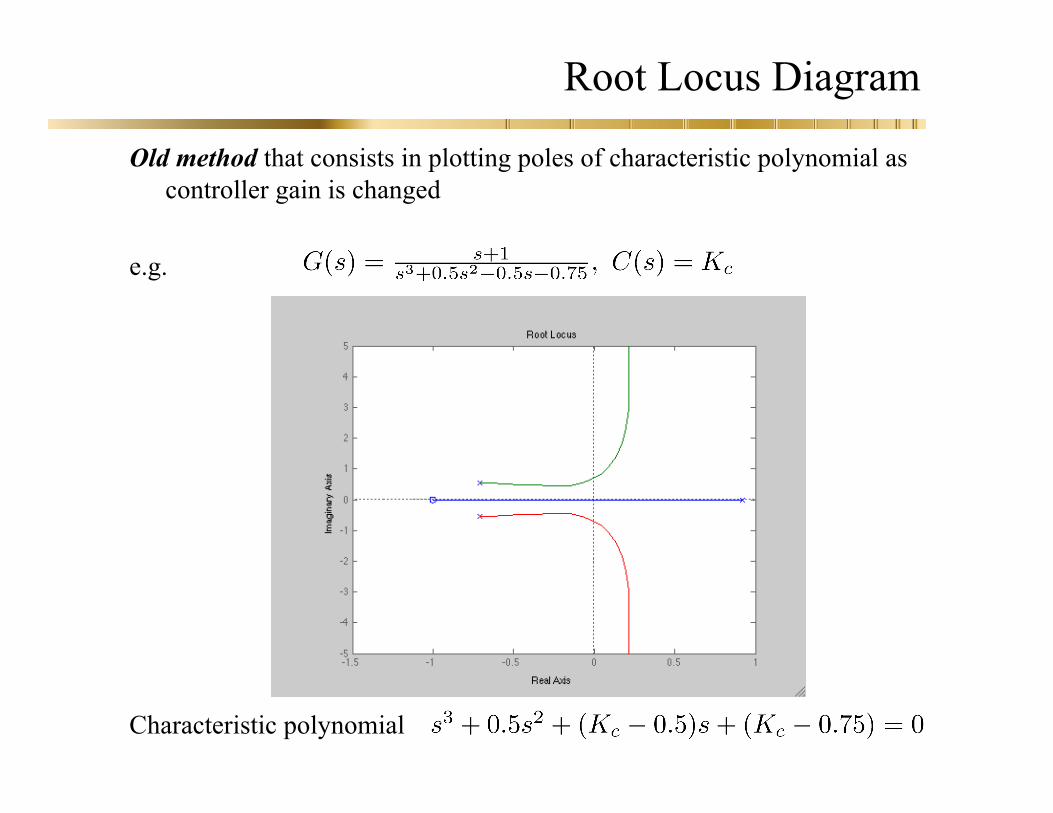
Root Locus Diagram
Old method that consists in plotting poles of characteristic polynomial ascontroller gain is changed
e.g.
Characteristic polynomial
51
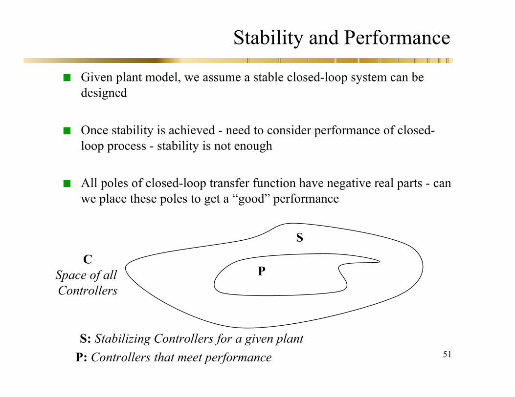
Stability and Performance
Given plant model, we assume a stable closed-loop system can bedesigned
Once stability is achieved - need to consider performance of closed-loop process - stability is not enough
All poles of closed-loop transfer function have negative real parts - canwe place these poles to get a “good” performance
S: Stabilizing Controllers for a given plantP: Controllers that meet performance
S
PC
Space of all Controllers
52
Controller Tuning
Can be achieved by Direct synthesis : Specify servo transfer function required and calculate
required controller - assume plant = model
Internal Model Control: Morari et al. (86) Similar to direct synthesisexcept that plant and plant model are concerned
Pole placement
Tuning relations:Cohen-Coon - 1/4 decay ratiodesigns based on ISE, IAE and ITAE
Frequency response techniquesBode criterionNyquist criterion
Field tuning and re-tuning
53
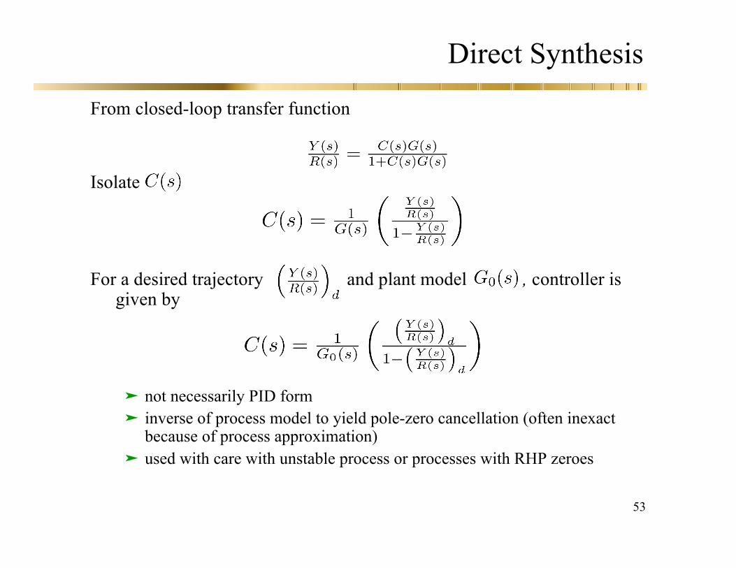
Direct Synthesis
From closed-loop transfer function
Isolate
For a desired trajectory and plant model , controller isgiven by
not necessarily PID form inverse of process model to yield pole-zero cancellation (often inexact
because of process approximation) used with care with unstable process or processes with RHP zeroes
54
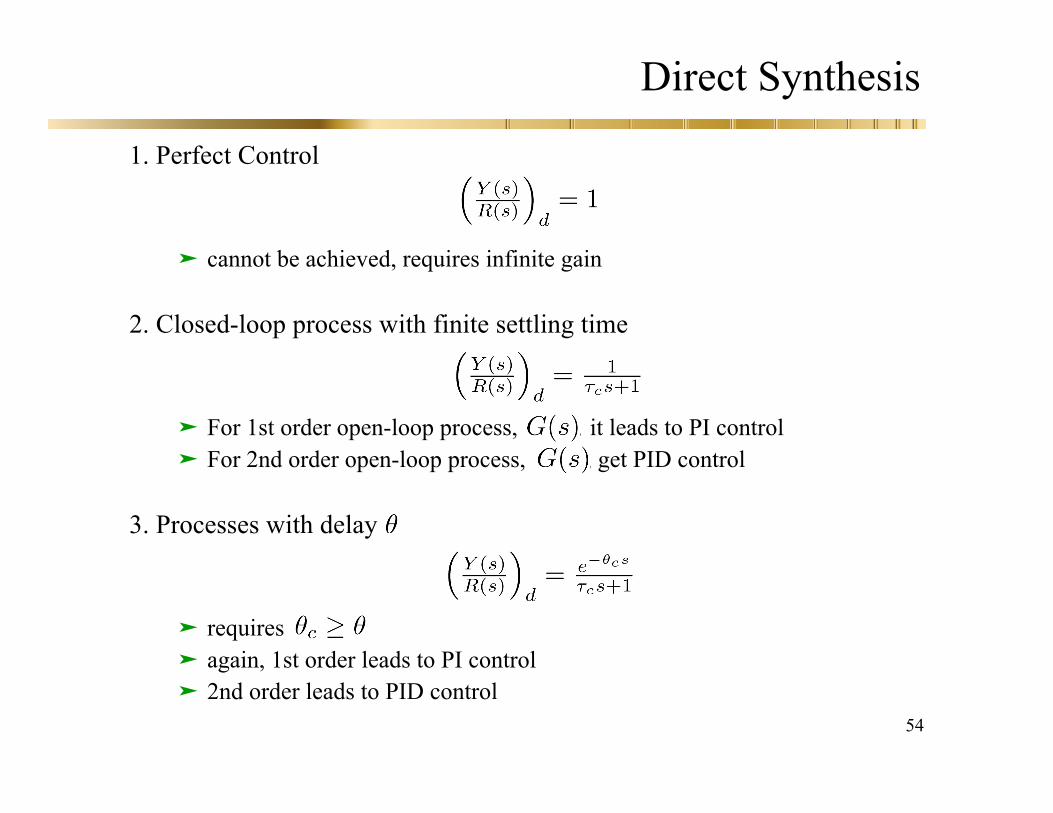
Direct Synthesis
1. Perfect Control
cannot be achieved, requires infinite gain
2. Closed-loop process with finite settling time
For 1st order open-loop process, , it leads to PI control For 2nd order open-loop process, , get PID control
3. Processes with delay
requires again, 1st order leads to PI control 2nd order leads to PID control
55
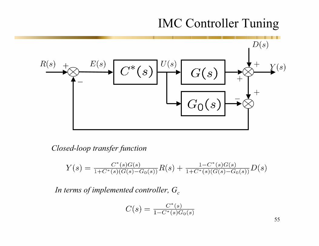
IMC Controller Tuning
Closed-loop transfer function
In terms of implemented controller, Gc
56
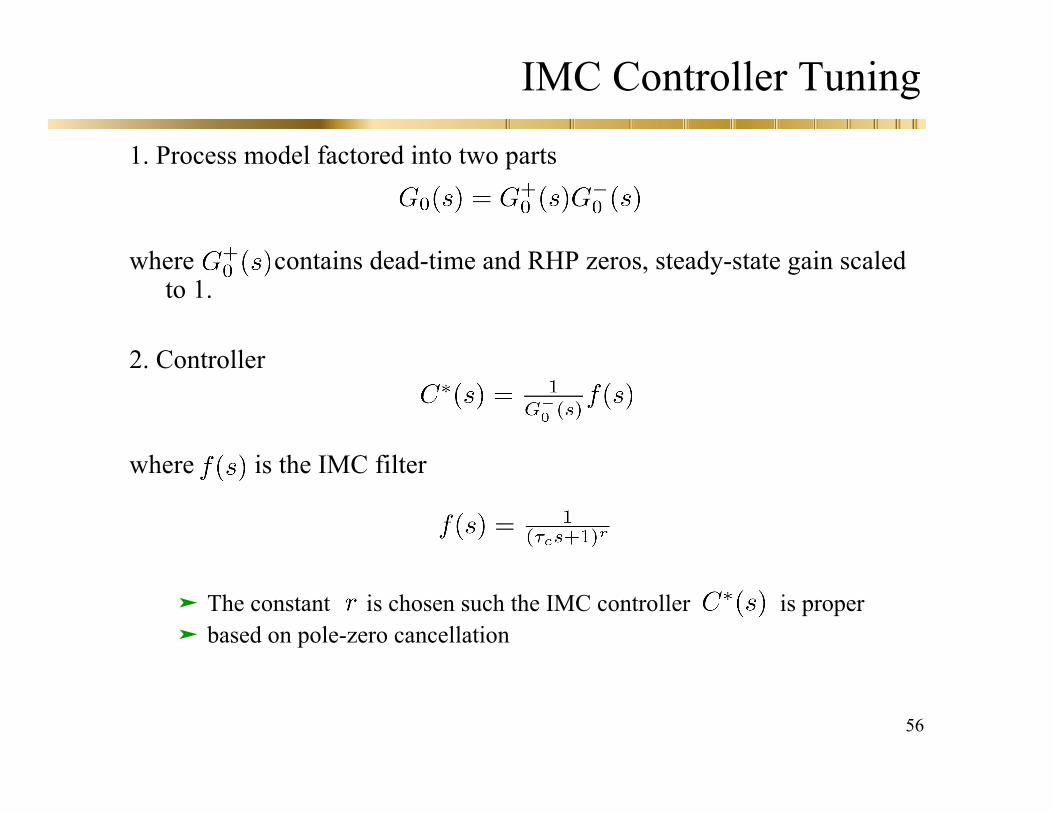
IMC Controller Tuning
1. Process model factored into two parts
where contains dead-time and RHP zeros, steady-state gain scaledto 1.
2. Controller
where is the IMC filter
The constant is chosen such the IMC controller is proper based on pole-zero cancellation
57
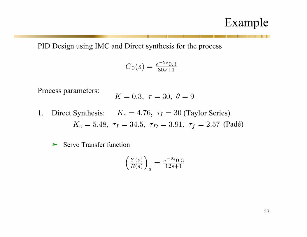
Example
PID Design using IMC and Direct synthesis for the process
Process parameters:
1. Direct Synthesis: (Taylor Series) (Padé)
Servo Transfer function
58
ExampleExample
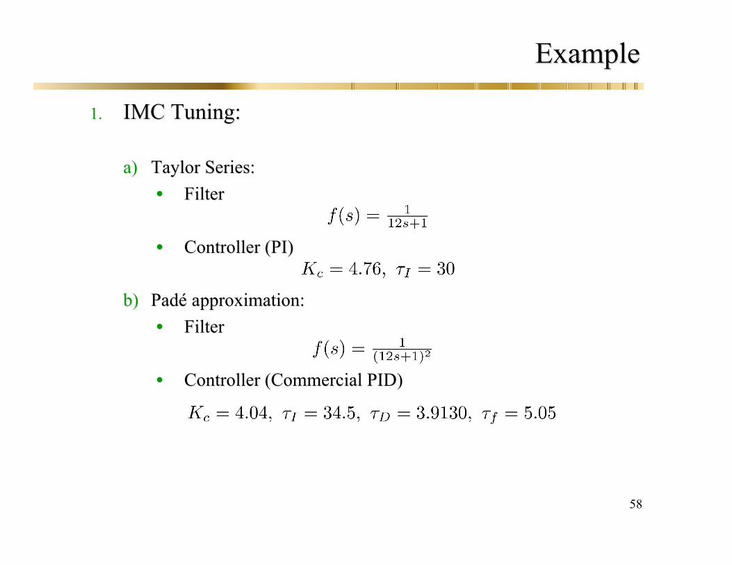
1.1. IMC Tuning:IMC Tuning:
a)a) Taylor Series:Taylor Series:•• FilterFilter
•• Controller (PI)Controller (PI)
b)b) PadPadé é approximation:approximation:•• FilterFilter
•• Controller (Commercial PID)Controller (Commercial PID)
59
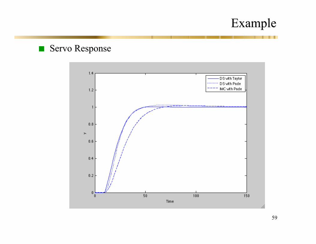
ExampleExample
Servo ResponseServo Response

60
ExampleExample
Regulatory responseRegulatory response
61
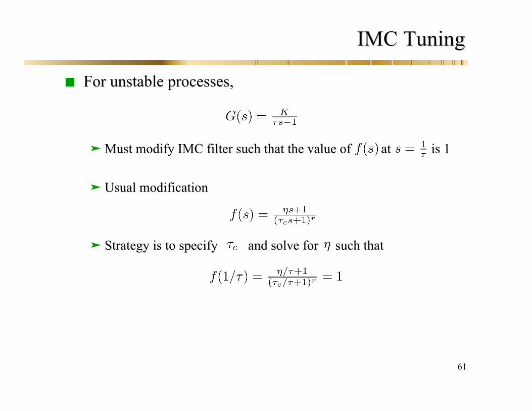
IMC TuningIMC Tuning
For unstable processes,For unstable processes,
Must modify IMC filter such that the value of atMust modify IMC filter such that the value of at is 1is 1
Usual modificationUsual modification
Strategy is to specifyStrategy is to specify and solve forand solve for such thatsuch that
62
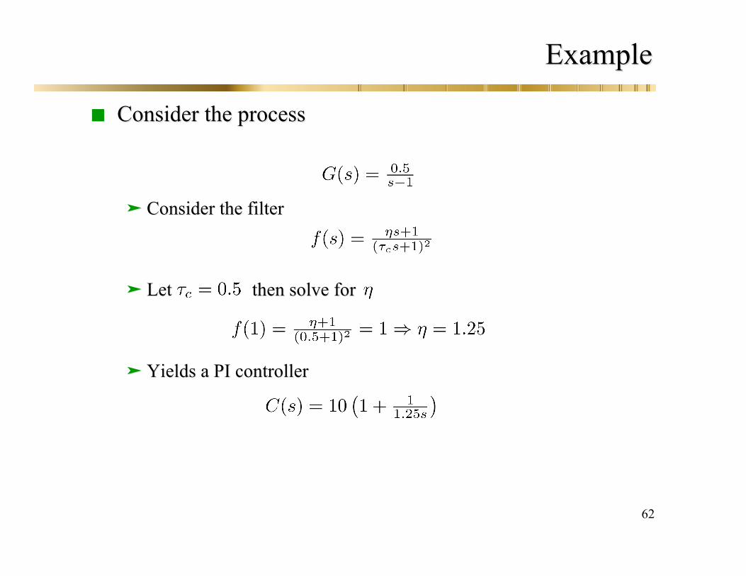
ExampleExample
Consider the processConsider the process
Consider the filterConsider the filter
Let then solve forLet then solve for
Yields aYields a PI controllerPI controller
63
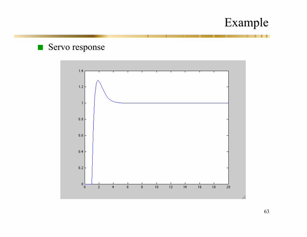
ExampleExample
Servo responseServo response
64
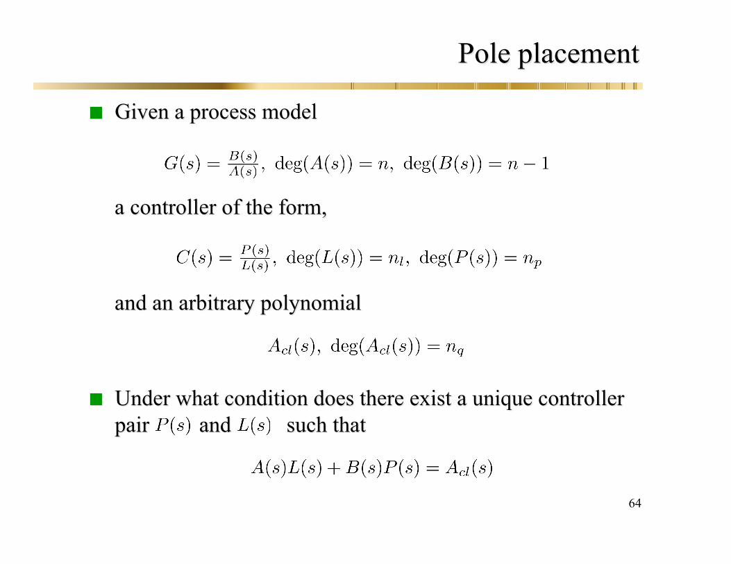
Pole placementPole placement
Given a process modelGiven a process model
a controller of the form,a controller of the form,
and an arbitrary polynomialand an arbitrary polynomial
Under what condition does there exist a unique controllerUnder what condition does there exist a unique controllerpair and such thatpair and such that
65
Pole placementPole placement
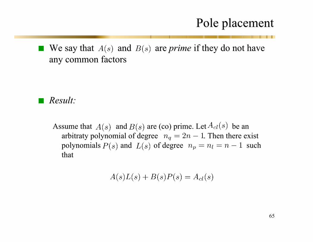
We say thatWe say that andand are are primeprime if they do not have if they do not haveany common factorsany common factors
Result:Result:
Assume that Assume that and and are (co) prime. Let are (co) prime. Let be anbe anarbitraty arbitraty polynomial of degreepolynomial of degree . Then there exist. Then there existpolynomialspolynomials and of degreeand of degree suchsuchthatthat
66
Pole PlacementPole Placement
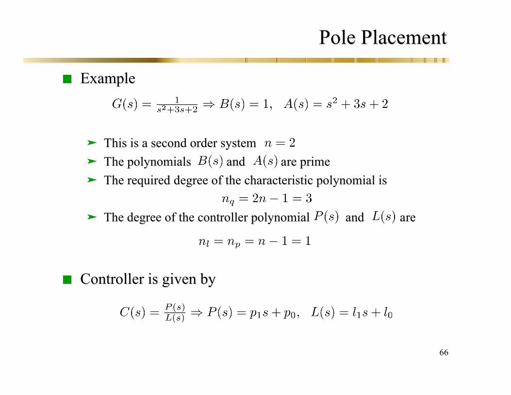
ExampleExample
This is a second order systemThis is a second order system The polynomialsThe polynomials andand are primeare prime The requiredThe required degree of the characteristic polynomial isdegree of the characteristic polynomial is
The The degree of the controller polynomialdegree of the controller polynomial andand areare
Controller is given byController is given by
67
Pole PlacementPole Placement
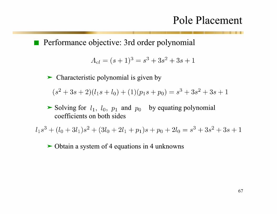
Performance objective:Performance objective: 3rd order polynomial3rd order polynomial
Characteristic polynomialCharacteristic polynomial is given byis given by
Solving forSolving for and and by equating polynomialby equating polynomialcoefficients on both sidescoefficients on both sides
Obtain a system of 4 equations in 4 unknownsObtain a system of 4 equations in 4 unknowns
68
Pole PlacementPole Placement
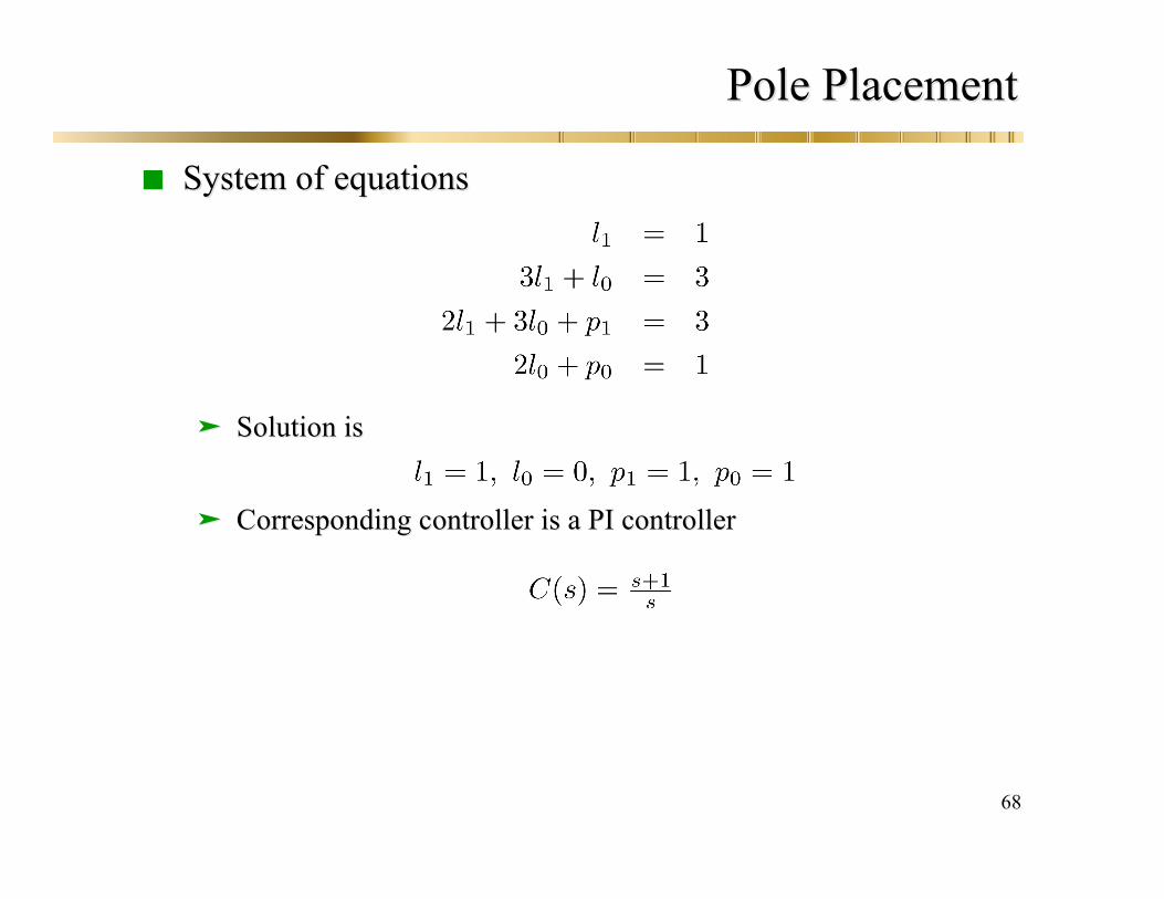
System of equationsSystem of equations
Solution isSolution is
CorrespondingCorresponding controller is a PI controllercontroller is a PI controller
69
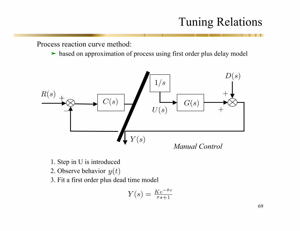
Tuning Relations
Process reaction curve method: based on approximation of process using first order plus delay model
1. Step in U is introduced2. Observe behavior3. Fit a first order plus dead time model
Manual Control
70
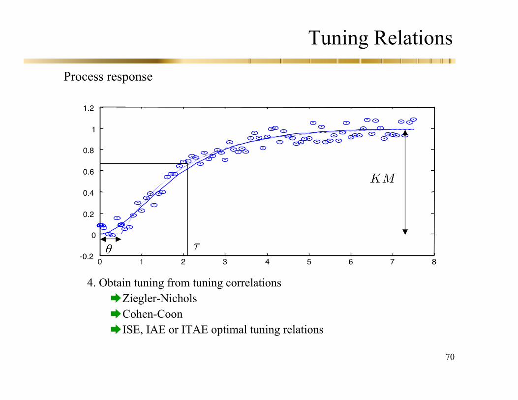
Tuning Relations
Process response
4. Obtain tuning from tuning correlationsZiegler-NicholsCohen-Coon ISE, IAE or ITAE optimal tuning relations
0 1 2 3 4 5 6 7 8-0.2
0
0.2
0.4
0.6
0.8
1
1.2
71
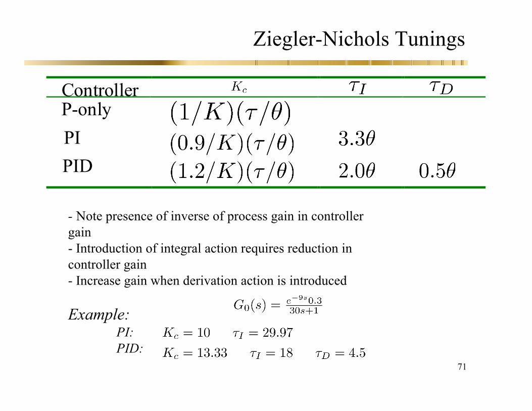
Ziegler-Nichols Tunings
Controller
PI-only
- Note presence of inverse of process gain in controllergain- Introduction of integral action requires reduction incontroller gain- Increase gain when derivation action is introduced
Example:PI:PID:
PID
P
72
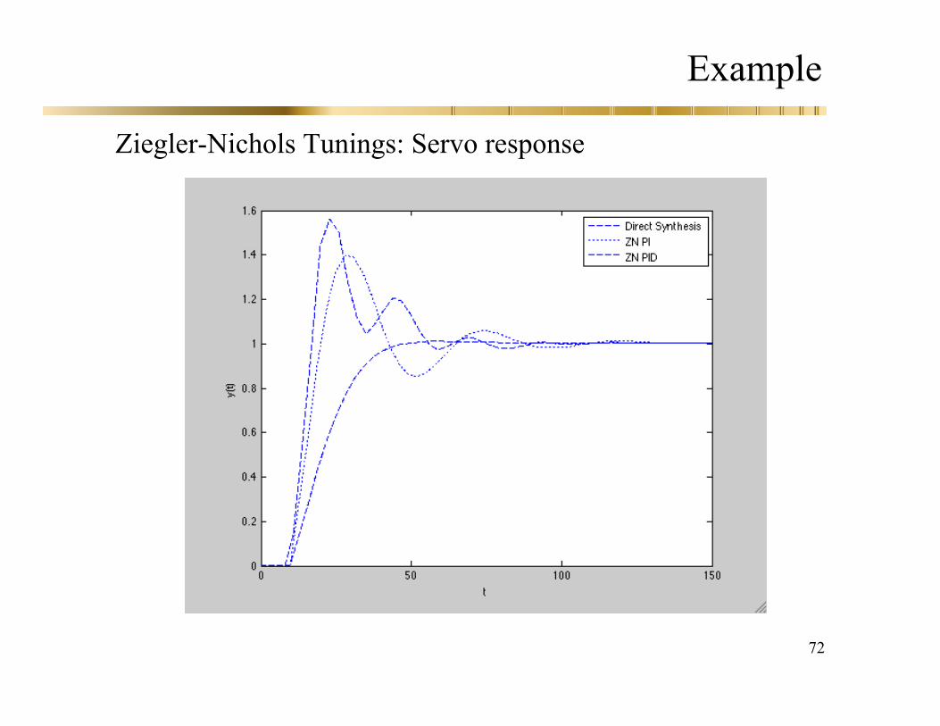
Example
Ziegler-Nichols Tunings: Servo response
73
Example
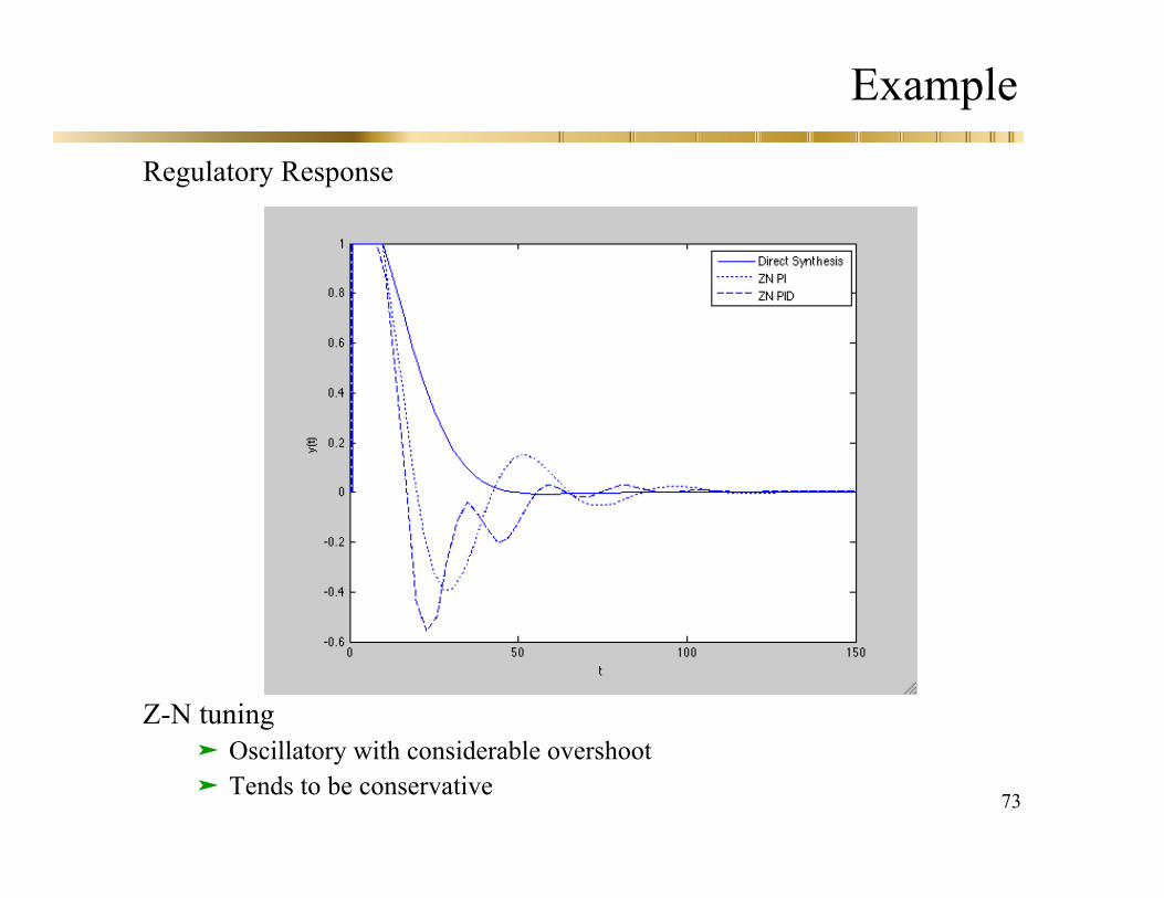
Regulatory Response
Z-N tuning Oscillatory with considerable overshoot Tends to be conservative
74
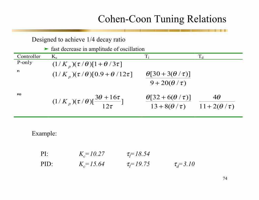
Cohen-Coon Tuning Relations
Designed to achieve 1/4 decay ratio fast decrease in amplitude of oscillation
Example:
PI: Kc=10.27 τI=18.54PID: Kc=15.64 τI=19.75 τd=3.10
Controller Kc Ti TdP-only ]3/1)[/)(/1( !""! +pKPI
]12/9.0)[/)(/1( !""! +pK)/(209)]/(330[
!"!""
++
PID
]12163
)[/)(/1(!
!""! +pK )/(813
)]/(632[!"!""
++
)/(2114
!""
+
75
Tuning relations
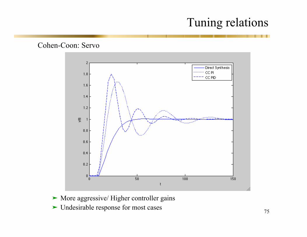
Cohen-Coon: Servo
More aggressive/ Higher controller gains Undesirable response for most cases

76
Tuning Relations
Cohen-Coon: Regulatory
Highly oscillatory Very aggressive
77
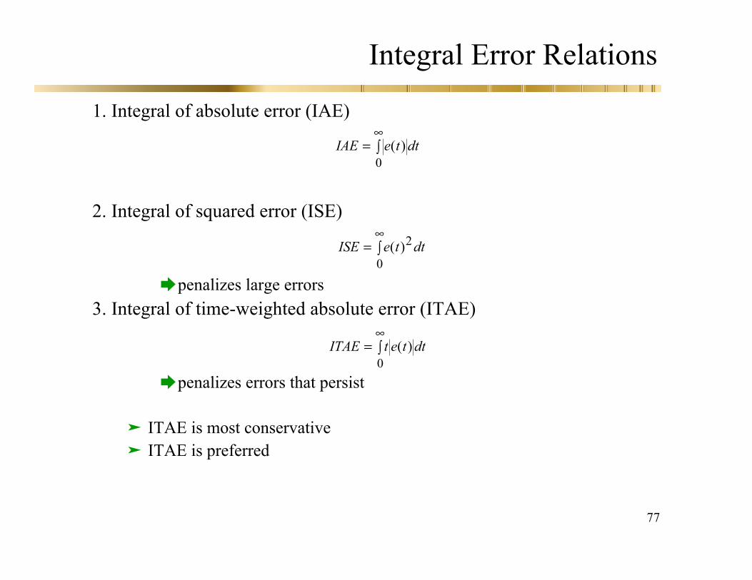
Integral Error Relations
1. Integral of absolute error (IAE)
2. Integral of squared error (ISE)
penalizes large errors3. Integral of time-weighted absolute error (ITAE)
penalizes errors that persist
ITAE is most conservative ITAE is preferred
ISE e t dt= !"( )2
0
ITAE t e t dt= !"( )
0
IAE e t dt= !"( )
0

78
ITAE Relations
Choose Kc, τI and τd that minimize the ITAE:
For a first order plus dead time model, solve for:
Design for Load and Setpoint changes yield different ITAE optimum
!!
!!"
!!"
ITAEK
ITAE ITAEc I d
= = =0 0 0, ,
Type ofInput
Type ofController
Mode A B
Load PI P 0.859 -0.977I 0.674 -0.680
Load PID P 1.357 -0.947I 0.842 -0.738D 0.381 0.995
Set point PI P 0.586 -0.916I 1.03 -0.165
Set point PID P 0.965 -0.85I 0.796 -0.1465D 0.308 0.929
79
ITAE Relations
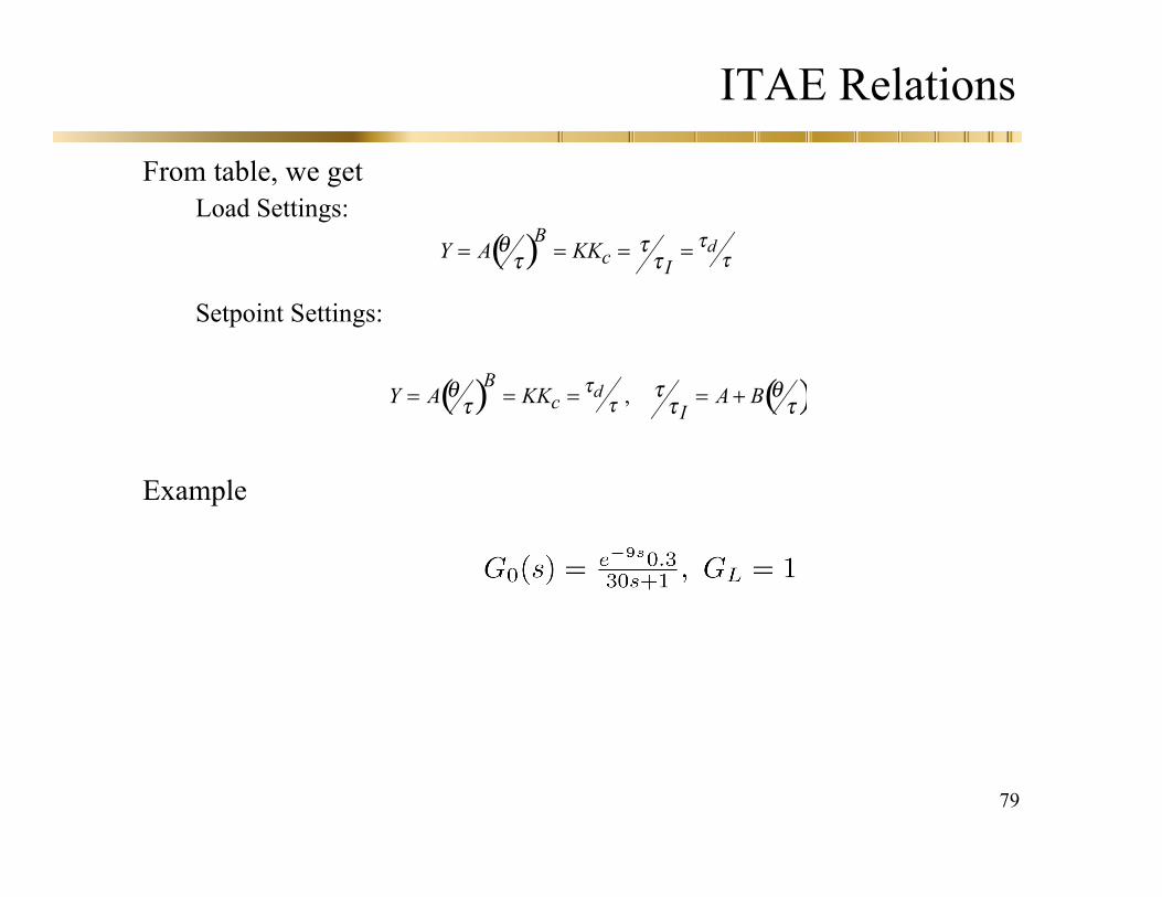
From table, we getLoad Settings:
Setpoint Settings:
Example
( ) ( )Y A KK A BB
c Id= = = = +!
"""
!"
"" ,
( )Y A KKB
c Id= = = =!
"""
""
80
ITAE Relations
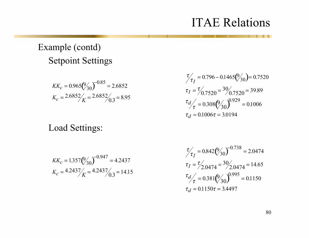
Example (contd)Setpoint Settings
Load Settings:
( )KK
K K
c
c
= =
= = =
!1357 4 2437
4 2437 4 24370 3 1415
930
0 947. .
. .. .
.( )
( )
!!
! !
!!
! !
I
I
d
d
= =
= = =
= =
= =
"0842 2 0474
2 0474302 0474 14 65
0 381 930 01150
01150 34497
930
0 738
0 995
. .
. . .
. .
. .
.
.
( )KK
K K
c
c
= =
= = =
!0 965 2 6852
2 6852 2 68520 3 8 95
930
085. .
. .. .
.( )
( )
!!
! !
!!
! !
I
I
d
d
= " =
= = =
= =
= =
0 796 01465 0 7520
0 7520300 7520 39 89
0 308 930 01006
01006 30194
930
0 929
. . .
. . .
. .
. .
.
81
ITAE Relations
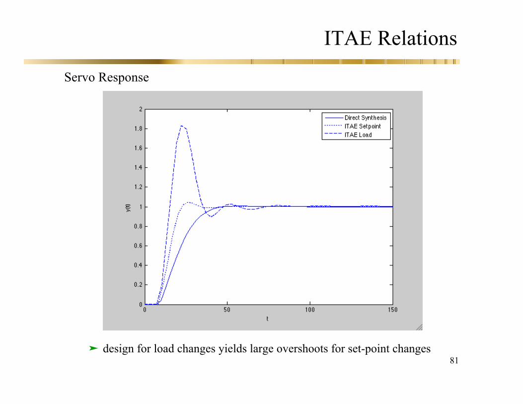
Servo Response
design for load changes yields large overshoots for set-point changes
82
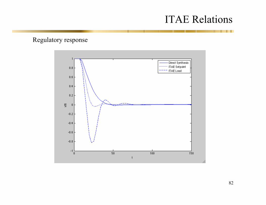
ITAE Relations
Regulatory response
83
Tuning Relations
In all correlations, controller gain should be inversely proportional toprocess gain
Controller gain is reduced when derivative action is introduced
Controller gain is reduced as increases
Integral time constant and derivative constant should increase asincreases
In general,
Ziegler-Nichols and Cohen-Coon tuning relations yield aggressivecontrol with oscillatory response (requires detuning)
ITAE provides conservative performance (not aggressive)
!"
!"
!!
dI= 0 25.