Federal Reserve Bank of Dallas

presents

RESEARCH PAPER

No. 9310

Does It Matter How Monetary Policy is Implemented?

by

Joseph H. Haslag, Research DepartmentFederal Reserve Bank of Dallas

and

Scott E. Hein, Finance DepartmentTexas Tech University

March 1993

This publication was digitized and made available by the Federal Reserve Bank of Dallas' Historical Library (FedHistory@dal.frb.org)

Federal Reserve Bank of Dallas

presents

RESEARCH PAPf:lfl

No. 831m

Does It Matter How Monetary Policy is Implemented?

by

Joseph H. Haslag, Research DepartmentFederal Reserve Bank of Dallas

and

Scott E. Hein, Finance DepartmentTexas Tech University

March 1993

Does It Matter How Monetary Policy is Implemented?

Joseph Haslag, Research DepartmentFederal Reserve Bank of Dallas

and

Scott Hein, Finance DepartmentTexas Tech University

The views expressed in this article are solely those of the authors and shouldnot be attributed to the Federal Reserve Bank of Dallas or to the FederalReserve System.

*

Does It Matter How Monetary Policy is Implemented?

Joseph H. Haslag*

and

Scott E. Hein**

Abstract: In the U.S., existing monetary base measures add anadjustment factor for changes in reserve requirementratios to high-powered money, de facto treating thepolicy actions as having the same effect. Yet, theorypredicts that the effects of changes in reserverequirements on prices and output are different fromthe effects of changes in high-powered money. Weestimate structural VARs, looking at the degree towhich the Fed offsets changes in reserve requirementsand whether the policy actions have differentialeffects on output growth and inflation.'

Research Department, Federal Reserve Bank of Dallasand Department of Economics, Southern Methodist University

•• First National Bank at Lubbock Distinguished Professor,Finance Department, Texas Tech University

, The authors gratefully acknowledge helpful suggestionsand comments from Sadhara Alanger, John Duca, Jerry Dwyer, KenEmery, Scott Freeman, Bill Gavin, Greg Huffman, Evan Koenig, JeffMercer, Allan Meltzer, Mark Wynne, and participants at the TexasTech Finance workshop. Of course, any errors are solely our own.We would also like to thank Ben Bernanke for providing hisprograms to estimate the structural VAR. The views expressedherein do not necessarily represent the views of the FederalReserve Bank of Dallas nor the Federal Reserve System.

1. Introduction

Monetary policy in the U. S. is implemented through open

market operations, discount window borrowings, and changes in

reserve requirement ratios. In open market operations and

discount window borrowings, the monetary authority changes

nominal balance-sheet quantities. In contrast, changes in

reserve requirement ratios represent a tax on intermediated

deposits. since the tools differ in this regard, there is a

natural question as to whether the economic response depends on

how monetary policy implemented. Yet, Federal Reserve system

monetary base measures do not differentiate between the three

tools. Implicitly, the monetary base measure treats changes in

reserve requirement ratios as having the same effects as changes

in nominal quantities due to open market operations or discount

window borrowing. By using the monetary base measure as the

chief policy indicator, one presumes that the economic effects of

the alternative policy tools are quantitatively similar. Plosser

(1989) explicitly questions the validity of this restriction:

" ..•monetary base numbers are peculiar mixtures of real and

nominal elements of monetary policy. The practice of adjusting

the base figures for reserve requirement changes confuses real

and nominal disturbances" (p. 261).2

2 Plosser (1989) and Haslag and Hein (1992) have separatelyprovided evidence suggesting that differences emerge in Grangercausality tests. For example, changes in reserve requirementshelp to predict changes in both output growth and inflation,whereas changes in high-powered money growth only help to predictchanges in inflation.

1

The importance of the monetary base in policy discussions

has increased over recent years. Brunner (1981), Meltzer (1984),

Poole (1982), Friedman (1984), and McCallum (1988) have argued

that the monetary base should be the centerpiece of monetary

policy. But, are the quite diverse monetary policy tools

adequately summarized in one measure?' If the answer to this

question is yes, the implication is that policymaker need not

care how monetary policy is implemented because the effects of

are similar. Consequently, the amalgam monetary base measure

adequately captures the thrust of alternative policy actions. In

contrast, using the monetary base in empirical analysis is not as

problematic if the evidence suggests that changes in reserve

requirement ratios have the same effect as changes in high-

powered money.

In addition to the policy implications, the monetary base is

frequently used in empirical studies. By not separating out the

effects of changes in reserve requirement ratios and high-powered

.money,.empirical work using adjusted monetary base measures

, Some people might suggest looking solely at the FederalReserve's balance sheet, considering high-powered money. Thepotential problem is that high-powered money could omit importantinformation in the conduct of monetary policy. Haslag and Hein(1989) provide evidence consistent with the notion that changesin high-powered money are coordinated with changes in reserverequirements. Focusing on high-powered money would give adistorted view of monetary policy for those cases: a decrease inhigh-powered money signals a contractionary monetary policyaction. Now suppose that the open market sale offsets a lowerreserve requirements. More will said of this type of coordinatedmonetary policy when we directly test the hypothesis that the Feduses open market operations to offset changes in reserverequirements.

2

implicitly impose the condition that the effects of changes in

reserve requirement ratios and changes in high-powered money base

are equal.

The purpose of this paper is to empirically investigate

whether the macroeconomic effects of changes in the Federal

Reserve's balance sheet--high-powered money--are significantly

different from the effects of changes in reserve requirement

ratios. Plosser (1989) and Haslag and Hein (1992) find that

different policy actions have different predictive qualities in

atheoretical macroeconomic settings. In contrast to those

earlier works, our focus is on interpreting structural

differences.' Here, the competing hypothesis--whether

differential output growth or inflation effects are indicated in

the data--is tested, using a structural VAR. More specifically,

we test the validity of the equality restriction imposed in the

monetary base measures, focusing on the monetary policy effects

on real GOP growth and inflation, both contemporaneously and over

time.

Two main findings are presented in this paper. First, we

find evidence that the Fed systematicallY offsets changes in

reserve requirements with changes in high-powered money. Thus,

the Fed smooths the effects of changes in its blunt instrument--

reserve requirements--with open market operations. For example,

• Here, we use the term structural in the sense that themodel is motivated by explicit economic theory [see Bernanke(1986)] .

3

the Fed partially offsets the amount of reserves freed by

lowering reserve requirements with open market sales. Hence, the

net effect of lowering reserve requirements is a higher growth

rate for the monetary base, but not as much as would be suggested

by isolated analysis of reserve requirement changes.

Second, the data are consistent with the hypothesis that

there are significant differential effects on both inflation and

output growth. These differences are not indicated in the

contemporaneous relationships, but emerge over time. Thus, the

empirical results suggest that the way in which monetary policy

is implemented does matter in the sense that the paths of output

growth and inflation differ (significantly) when one changes the

contribution to monetary base growth from reserve requirements

and high-powered money by equal magnitudes.

The paper is organized as follows. In section 2, the

literature is reviewed and the testable hypothesis are

identified. We empirically test the restriction that changes in

reserve requirement ratios are equal to changes in high-powered

money in section 3. In addition, we specify alternative models

to check the robustness of the findings. The dynamic responses

are plotted and discussed in section 4. section 5 provides a

brief summary of the results.

2. competing Hypotheses

Do changes in reserve requirements and high-powered money

have equal-sized effects on prices? The theoretical literature

4

appears split on this issue. Romer (1985) examines this question

in a general equilibrium model. He finds that an increase in the

reserve requirement does not affect steady state inflation (p.

183). In contrast, Romer's model predicts that changes in high­

powered money do affect the inflation rate.

Freeman (1987) specifies an overlapping-generations model in

which reserve requirements are necessary for agents to hold fiat

money. Both capital and government bonds offer strictly higher

rates of return. Using Freeman's model, however, one can show

that the elasticity of the inflation rate to a change in reserve

requirements is equal to the elasticity to a change in high­

powered money.

These studies establish the null and alternative hypotheses

for the effects of changes in reserve requirements on inflation.

In short, Freeman's model predicts that changes in reserve

requirements and changes in high-powered money will have equal­

sized effects on the inflation rate. This model provides a

theoretical justification for adding the reserve adjustment

measures to high-powered money, as is currently done. This is

the null hypothesis in our subsequent empirical work.

Conversely, the Romer model predicts differential effects for the

different policy actions, establishing the basis for the

alternative hypothesis.

Another empirical issue is the relationship between high­

powered money and changes in reserve requirements. Dwyer and

Saving (1986) describe the government as having a patent on money

5

creation. In this framework, reserve requirements serve as a

licensing fee. Dwyer and Saving argue that the government's

revenue from money creation is independent of whether base money

is issued directly or created through the banking system. In

their setup, the licensing fee establishes the allocation of

revenues between government and public sources, but does not

affect the size of the revenues. In other words, the government

can generate the same amount of seignorage revenue with a lower

growth rate of high-powered money growth when reserve

requirements are lowered. Therefore, Dwyer and Saving provide a

theoretical justification for a relationship between reserve

requirements and high-powered money in which both are tools

capable of generating seignorage revenue.

In practice, Dwyer and Saving's model predicts that, for a

given level of seignorage revenue, the Fe~ systematically offsets

changes in reserve requirements with open market operations.'

Hence, there is some coordination between the different monetary

policy actions. However, the standard textbook of monetary

policy examines the effects of each policy action as if reserve

requirements and open market operations are conducted

independently. Here, the null hypothesis is that monetary policy

actions are not coordinated. If a relationship is evident in the

, Muelendyke (1992) states that the Fed does offset changesin reserve requirements with open market operations. Haslag andHein (1989) provide evidence that a negative correlation betweenhigh-powered money and the st. Louis reserve adjustment magnitUde(RAM) is present.

6

structural model, the question then is whether the offset is full

or partial.

Table 1 presents the null hypothesis that we explicitly test

in the paper. As Table 1 shows, we concentrate on three main

hypothesis in our empirical work. These hypothesis bear on the

issue of whether the adjusted monetary base measures are

justified to add the reserve adjustment measure and high-powered

money. In addition to the two hypothesis regarding the effects

on inflation and the simultaneous policy actions (H1 and H2), we

consider the hypothesis of equal-sized effects on output growth

denoted H3. 67 The next section implements the strategy to test

these hypothesis.

6 Champ and Freeman (1990) find that high-powered money andreserve requirements will have differential effects on investmentand output, deriving a closed-form solution for the capitalstock. Champ and Freeman assume that agents have a requiredreserves constraint, not a percentage-of-intermediated depositconstraint. For our purposes, finding differential effects issufficient to motivate the empirical investigation.

7 A literature has developed that examines whether reserverequirements affect the stability of output. The modelsgenerally focus on the 0 and 100 percent reserve requirementcases. The basic idea is that reserve requirements stabilize thedemand for money, and mitigate the transmission of monetaryshocks to the real sector. Baltensperger (1982), for example,finds that reserve requirements do stabilize the money stock, butnot necessarily increase the stability of output growth andinflation. Horrigan (1988) argues that, in general, reserverequirements do affect output variability. However, when thegovernment targets interest rates, he finds that reserverequirements are irrelevant for economic stabilization. Thesehypothesis are explicitly about the relationship between thevariance of output and reserve requirements. Here, we are moreinterested in the differential effects on the level of outputgrowth, if any, resulting from changes in reserve requirementsand changes in high-powered money growth.

7

3. Model Estimation

In this section, we estimate structural VARs to test whether

the changes in reserve requirements and changes in high-powered

money have the same effects on economic activity. We consider

several different sets of identifying assumptions, thereby

checking the robustness of the results. In addition to looking

at the contemporaneous coefficients estimated in the particular

orthogonalization, we use impulse response functions to consider

if dynamic differences are suggested by the data.

Three main hypothesis are tested in the empirical section:

(i) to what extent, if any, does the Fed systematically offset

changes in reserve requirements with open market operations; (ii)

is the effect of a change in reserve requirements significantly

different from the effect of a change in high-powered money; and

(iii) is the effect of a change in reserve requirements

significantly different from the effect of a change in high­

powered money. The last two questions bear directly on whether

one should use a simple sum approach when constructing the

monetary base. Since the monetary base is used extensively in

empirical work, the answer could support this practice or could

raise serious questions regarding the appropriate interpretation

of results obtained with the simple sum measure.

3.1 Data and Related Issues

The conventional measure of changes in reserve requirement

ratios is the reserve adjustment magnitude (RAM) constructed by

the Federal Reserve Bank of st. Louis. Formally, RAMt = (rb -

8

r<) 'D<, where r is a Kx1 vector of reserve requirement ratios and

D is a Kx1 vector of deposit types against which reserves must

legally be held. The sUbscript b refers to the period identified

as the base period and t denotes the current time period. RAM

not only changes when changes in reserve requirement ratios

occur, but RAM also changes when deposit levels change,

reflecting changes in the vector of deposit types, as long as r b

¢ r<. Haslag and Hein (1993) have constructed an alternative

measure that separates out changes in RAM due to changes in

deposits from changes in reserve requirement ratios. Like RAM,

the Haslag-Hein measure--denoted RSI--adds high-powered money to

the reserve adjustment factor, imposing the condition that a $1

increase in high-powered money is equivalent to $1 freed by lower

reserve requirement ratios.

Formally, ARSI< = r<' D< - r<-1' D<-1 (where A is the difference

operator) for the week in which changes in reserve requirement

ratios occur. It is easy to show that ARAM< = r b' AD< - ARSI< for

periods in which changes in reserve requirement occur and A~ =

rb'AD< - r<'AD< for periods in which no changes in reserve

requirement ratios occur. We use RSI as our measure throughout

the empirical analysis because changes in this measure are

straightforwardly interpreted as changes in reserve requirement

ratios. The data used in this investigation are quarterly and

9

are, except for RSI, seasonally adjusted."

Following the definition of the monetary base, high-powered

money growth and RSI growth are defined in (centered) percentage-~

change form relative to the monetary base; that is, H t = 4H/[(MBt

+ MBt _,)/2] and RSl t = 4RSlf[(MBt + MBt _ 1 )/2], respectively, where H

denotes the level of high-powered money and MB is the monetary

base. These two variables are used separately in explaining

macroeconomic behavior. The measure of output is real GDP, while

inflation is measured as the fixed-weight GDP deflator

(1982=100).

One property of our definition of the monetary base

components is that permanent changes in reserve requirements show

up as one-time changes in RSI, and hence, RSI. Note that RSI

will follow a pattern identical to a series with infrequent,

permanent shocks. Balke and Fomby (1992) show that one will fail

to reject the hypothesis of a unit root in time series subject to

infrequent, permanent shocks. Constructing our series in

percentage-change form relative to the monetary base serves two

purposes. First, and most important, the approach permits us to

directly test whether a change in monetary base due to a change

in reserve requirements has a different effect on macroeconomic

" See Haslag and Hein for a detailed description of the RSImeasure. We also used the st. Louis RAM to capture the effectsof changes in reserve requirements. RSI is not seasonallyadjusted since there is no apparent seasonality regarding whenthe Fed elects to change reserve requirements. The main findingsreported in this paper are not affected by substituting RAM forRSI. Tables and charts using RAM instead of RSI are availablefrom the authors upon request.

10

variables under the assumption that the monetary base should beA A

constructed as a simple-sum measure. Second, both RSI and Hare

stationary series."

3.2 Estimation methodology

The estimation procedure is the structural VAR methodology

presented in Blanchard and Watson (1986), Bernanke (1986), and

Sims (1986). The procedure is employed in two estimation steps.

The first step involves estimating a vector autoregression which

is represented as:

(9)

where Xc = [RSI c He mm2 c INFc GOP c ], where mm2 is the growth rate

of the M2 money mUltiplier, INF is inflation measured by theA

fixed-weight deflator, GOP is real GOP growth, 4 is the number

of lagged values included, a is the estimated vector of reduced-

form coefficients, and Uc is the vector of reduced-form

residuals.

In the second step, recall that one can represent the

product of structural parameters and the reduced-form errors, u c '

as the structural disturbances (see Bordo, Schwartz, and

• Sims, Stock, and Watson (1990) state the conditions inwhich statistical inference is valid with non-stationary series.While we may suffer from over-differencing from the standpoint ofthe effects on output and prices, the contributions to monetarybase growth due to RSI and high-powered money are appropriate forlooking at output growth and inflation.

11

Rappaport (1991), for example); that is, the errors from the

structural equations. Formally, let v< denote the "structural"

disturbances. The reduced-form errors are characterized as v< =

then use the observed, reduced-form error terms and the

identifying assumptions to estimate the structural coefficients.

The reduced-form error terms are conceptually constructed as

unanticipated innovations to the series. Thus, the identifying

restrictions are applied to testing the effects of unanticipated

innovations on variables and represent a rational expectations

model. 10

Table 2 reports the findings from the exclusion restrictions

obtained from estimating the first step, namely estimating the

unrestricted VAR using four lagged values of the variables. For

each variable in the system, the null hypothesis is that

coefficients on the lagged values of the excluded variable (the

column heading) are jointly equal to zero. The row heading

identifies the equation in which we are testing the exclusion

hypothesis. Table 2 presents the results obtained when one uses

10 Blanchard and Quah (1989) looked at a structural VAR inwhich they identified permanent and temporary shocks to output.King, Plosser, Stock and Watson (1991) extended Blanchard andQuah to consider the presence of cointegrating relationshipsbetween the series in the structural VAR. In this way, the dataidentified long-run relationships. Here, we use contemporaneousidentifying restrictions in our analysis. We tested forcointegrating relationships between the policy variables (whichare non-stationary in levels) and output and prices. Theevidence does not support the existence of a long-runrelationship of this sort between the policy variables andeconomic activity.

12

the VAR system described above.

For the null hypothesis that changes in reserve requirement

ratios help predict changes in output growth, the F-statistic is

4.01. The five-percent critical value is 2.45. Thus, the

evidence from Table 2 suggests that changes in reserve

requirement ratios do temporally precede movements in output

growth. This finding is similar to that of Haslag and Hein

(1992), although a different VAR system is specified and the

measure of reserve requirements (RAM vs. RSI) is different.

In addition, the reduced-form parameters suggest that

changes in source base growth provide predictive content for

future output growth as the F-statistic is 2.98. However, the F­

statistic is 1.37 under the null hypothesis that changes in high­

powered money help to predict changes in the inflation rate, (the

10-percent critical value is 1.99) rejecting the notion that

movements in high-powered money temporally precede changes in

inflation. There is also evidence suggesting that changes in the

M2 money mUltiplier temporally precedes changes in output growth

(the F-statistics is 4.62), but none of the money variables help

to predict changes in the inflation rate.

We estimate the following structural VAR (note that the

letter u with sUbscripted variable names represent the reduced­

form, or one-step-ahead forecast, errors from the first step

estimation). We hereafter refer to this specification as the

Control model:

13

(la) U RS1 = Zlt

(lb) Us = P, u RS ' + {3 2 u"",2 + {33 u 1NF + z2 t

(lc) u,."" = P4 U 1NF + {35 U GDP + z3 t

(ld) u 1NF = {36 U RS1 + {37 Us + z4 t

(le) UeDP = {3. U RS1 + P. u B + {3 IOu,."" + z5r.I

where u with a sUbscript denotes the innovation from the reduced­

form equation.

Equation (la) postulates that innovations in RSI are a

structural disturbance. Equation (lb) specifies that movements

in high-powered money respond contemporaneously to innovations in

RSI, indicating that changes in reserve requirement ratios are

contemporaneously offset ({3, < 0) by changes in high-powered

money. This specification examines the Fed's willingness to

coordinate different types of monetary policy actions;

specifically testing whether there is any contemporaneous

coordination of reserve requirement changes and money growth. If

so, the evidence gives further credence to the notion that the

monetary authority uses fiat money to offset the effects of

changes in reserve requirements. In addition, equation (lb)

specifies that high-powered money responds to movements in the

money mUltiplier. This specification can be motivated as the Fed

trying to aChieve its M2 target path. Hence, reductions in M2

money mUltiplier would be met be increases in base growth.

Equation (lc) is a money demand function. We postulate that

innovations in inflation and income affect the demand for M2

14

assets. We assume that innovations in the money multiplier do

not affect the inflation rate, but can affect the output."

Equations (ld) and (Ie) represent the contemporaneous models

of inflation and output growth, respectively. In these

specifications, we can test directly whether innovations in

reserve requirements and high-powered money have differential

contemporaneous effects.

The top portion of Table 3 reports the estimated

contemporaneous coefficients for the structural VAR described in

equations (la-e). Three key conclusions are illustrated in these

results. First, note the strong, negative coefficient on the

reserve requirement variable in the high-powered money equation.

The evidence, therefore, suggests that decreases in reserve

requirements, for example, are contemporaneously (within quarter)

offset by open market sales. Note also that the coefficient on

RSI is significantly less than one (in absolute values), so that

the Fed, on average, only partially accommodates changes in

reserve requirement ratios with open market operations. In other

words, changes in reserve requirements have an activist component

to them, but much less than suggested by this tool in isolation.

11 King and Plosser (1984) argue that base m~mey isresponsible for changes in prices. Movements in the moneymultiplier reflect "real" factors affecting output determination.Thus, a broader money measure (M2, for example, separated intoits base and money mUltiplier components) is the appropriatemeasure to gauge monetary policy in their real business cyclemodel. We consider the contemporaneous role of each component inaffecting output growth and inflation in other structural VARsthat are used to monitor the robustness of our findings.

15

Second, the coefficient on high-powered money in the

inflation equation is significant at the 10-percent level. The

coefficient on RSI is not significant even at marginal levels.

Under the null hypothesis that the coefficient on high-powered

money is equal to the coefficient on RSI, the t-statistic is

0.52. Hence, one cannot reject the null hypothesis that the

effects of changes in high-powered money have the same

contemporaneous effect on inflation as changes in reserve

requirement ratios.

Third, none of the variables are significant in the output

equation. Testing whether the coefficient on RSI is equal to the

coefficient on high-powered money, the t-statistic is 0.94. The

findings, therefore, indicate that neither RSI nor Hare

contemporaneously correlated with output growth. Moreover, the

effects of changes in reserve requirements and high-powered money

on output growth are not statistically differently from one

another.

The middle portion of Table 3 reports the estimated

contemporaneous coefficients for a modified version of the model

used in Sims (1986) paper. Here, the main modification to Sims

structure is that the M1 money supply is separated into its money

mUltiplier, high-powered money and RSI components. Other

differences include using the implicit price deflator as the

price measure and GNP as the output measure. In addition, the

sample period is 1948-90.

Generally, the results from the modified-Sims model support

16

the findings reported in the Control model. In particular, there

is a negative contemporaneous relationship between changes in

reserve requirements and changes in high-powered money. The

results from the modified-Sims model also indicate that the Fed

systematically and partially offsets the increase in monetary

base growth due lower reserve requirements by reducing the

contribution due to high-powered money growth. The modified-Sims

model excludes reserve requirements and high-powered money from

the output growth equation. In the inflation equation, neither

high-powered money nor RSI has a significant contemporaneous

relationship with inflation. More importantly for our purposes,

the coefficients are on RSI and H are not significantly different

from one another (t-value = -1.14).

Finally, we specify a third structural VAR, one in which

supply shocks playa prominent role. In particular, the relative

price of energy is included to account for the chief shocks

hitting the economy during the 1970s. The bottom portion of

Table 3 reports the contemporaneous effects from this supply­

shock model. As in the models above, changes in reserve

requirements are contemporaneously correlated with changes in

high-powered money and this is a partial offset. The evidence

indicates that general price level changes are not

contemporaneously related to changes in the relative price of

energy, suggesting that energy prices move one-for-one with the

price level (equation 2). In addition, inflation is posited as a

function of shocks to the relative price of energy and output

17

growth. Neither energy price shocks nor output growth

contemporaneously affect the inflation rate. Note that the

contemporaneous coefficients on high-powered money and the M2

money multiplier are significant and positively related to

changes in output growth.

We test for equal-sized coefficients on the monetary

variables in both the inflation and output growth equations. The

t-values calculated under the null that the contemporaneous

coefficient on RSI is equal to the contemporaneous coefficient on

Hare -0.80 and -0.67 for the inflation and output growth

equations, respectively.'2

In short, we find evidence suggesting that the Fed partially

offsets changes in reserve requirement ratios with open market

operations. Second, the evidence suggests that the

contemporaneous effects of changes in high-powered money growth

and RSI on either inflation or output growth are not

significantly different from one another.

4. Dynamic Responses

'2 We tried other structural VARs differing primarily interms of the contemporaneous reaction functions for both RSI andH. These structural VARs are not reported because they typicallydid not converge. The Bernanke procedure uses a nonlinearmethodology to solve the simultaneous equations. When the modelsdo not converge, standard errors are not obtained and thehypotheses in which we are interested cannot be tested.

Note further that the data do not include the interwarperiod (1929-45) which may be very different from the resultsobtained using postwar data. There is some conjecture that theFed used reserve requirement changes without offsetting openmarket operations during the 1930s.

18

We use impulse response functions to compare different

monetary policy actions over time. Milton Friedman (1969) gave

considerable support to these experiments when he concluded that

there is a lagged effect between monetary policy and changes in

economic activity. Thus, it is more likely that differential

effects present in the estimated relationships will show up in

effects over time rather than in the contemporaneous effects.

Two sets of experiments are investigated here. The first

set looks at the impulse responses for one-percentage-point

innovations to reserve requirements and high-powered money,

separately. The second set examines the responses to a

simultaneous changes in RSI and H such that monetary base is

constant. This second experiment takes into account the partial

accommodation observed in the structural model.

Here, the result that the Fed typically offsets changes in

reserve requirements with high-powered money has important

implications. The impUlse response function uses the

contemporaneous specifications (the identifying restrictions) and

the reduced-form models. One implication is that the impulse

response function is conceptually similar to a total derivative,

incorporating contemporaneous ("direct") channels and reduced­

form ("indirect") channels. For our purposes, the

contemporaneous relationship between high-powered money growth

and RSI indicates an immediate response by to innovations in RSI.

As such, the experiment with an innovation in RSI is not one in

which other monetary policy actions are held constant. In the

19

first set of experiments, we proceed with an innovation in RSI,

recognizing the partial offset in H is present.

4.1 rndependent monetary policy innovations

In the first experiment, innovations to RSI and to high­

powered money are considered. As we found in the contemporaneous

equations, a partial offset of changes in reserve requirements is

present. with this caveat, we interpret these results as the

effects of each policy action, holding the other policy action

constant. Such evidence bears indirectly on the issue of whether

the effects of the two policy actions are equal-sized. The

impulse responses, therefore, are illustrate the effects of each

action over time.

Chart 1 plots the dynamic response to a one-percentage-point

increase in RSI, which contributes a one-time change in monetary

base growth,' using the Control model. Ninety-percent confidence

intervals are included. The top panel in chart 1 is the

inflation-rate response. As the chart shows, the inflation-rate

responses are not significantly different from zero during the

first few quarters after the reserve requirement shock. However,

in the fifth quarter after the change in reserve requirements,

the inflation rate is significantly above zero, and the impulse

response function remains above zero for about ten quarters. The

interpretation is that a (one-time) one-percentage-point increase

in RSI (a decrease in reserve requirements) results in

temporarily higher inflation.

The bottom panel in Chart 1 plots the impulse response

20

function for output growth, again assuming a 1-percentage-point

increase in RSI and again using the Basic model. According to

the chart, during the first two quarters after the reserve

requirement shock, output growth is significantly higher. Thus,

the evidence supports the notion that a one-time change in the

reserve requirement ratio results a temporarily higher growth

rate in output. 13 This experiment takes into account the partial

offsetting of reserve requirement changes using open market

operations. Recall the theoretical model predicted that using

open market operations to partially offset changes in reserve

requirements would result in changes in both output growth and

inflation.

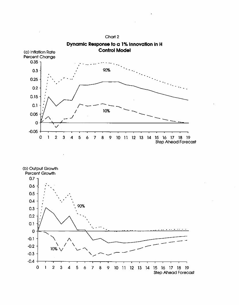
Chart 2 plots the dynamic responses given a one-percentage­

point increase in high-powered money. The top panel of Chart 2

shows the effects of the increase in high-powered money growth on

the inflation rate. As Chart 2 shows, the effect of higher base

money growth rises through the first few quarter, and decays

slowly as the impulse response function is still significantly

above zero 20 quarters after the innovation occurs.

Chart 2 also shows that the effect that an innovation to

high-powered money has on output growth. The bottom panel shows

13 Lougani and Rush (1991) find evidence that changes inreserve requirements do help to explain movements in outputgrowth and investment. Note that the path for investmentspending growth is qualitatively the same as output growth in allof our experiments. As such, our evidence lends further supportto Lougani and Rush. Note also that they use the ratio ofadjusted monetary base to high-powered money as their measure ofchanges in reserve requirements.

21

that increases in high-powered money have a negative effect on

output growth about 3 years after the innovation occurs. This

effect is significant at the 10 percent level (p-value is 0.097).

The economic interpretation is that a one-time change in high­

powered money growth has significant, temporary effects on output

growth, which first rises and then falls. Statistically, the

pattern of the response probably reflects the fact that the

innovation to high-powered money growth is stationary so that the

series tends towards it (sample) mean after an innovation occurs.

Charts 3 and 4 plot the same set of impulse response

functions presented in Charts 1 and 2, except now using the

modified-Sims structure and Supply-shock models, respectively.

The results from both models are qualitatively similar to those

reported in the Control model. There is some difference in the

timing of the significant effects, but the direction of the

significant effects match the main findings presented in the

Control model quite closely. The results from the supply-shock

differ somewhat. For example, there is no significant decline in

output growth to a one-percentage-point increase in RSI.

Just looking at the charts, it is striking how similar the

inflation rate and output growth responses are. Specifically,

the effects of a change in RSI and in high-powered money are

quite similar in shape and magnitude. Generally, the inflation

rate response peaks somewhere between the first and second year

after the innovation and then slowly decays. In addition, the

peak response is between 0.15 and 0.30 percentage points. This

22

pattern is observed regardless of whether the innovation is in

RSI or H.

The output growth responses are also quite similar to each

type of policy shock. Generally, the output growth response is

more like a cycle with the maximum effect observed two quarters

after the innovation and output growth falling below zero some

time after the first year post-innovation. The peak response is

typically between one-quarter and one-half a percentage point.

The similarity in magnitude and shape is, like the inflation rate

response, invariant to the source of the innovation.

The evidence thus far suggests that the two policy actions

have equal-sized effects. Clearly, what one would want is a test

in which equal-sized policy innovations are considered (either

independently or simultaneously). The experiments considered

thus far violate the standard of same-sized innovation, because

of the contemporaneous relationship between shocks to RSI and

high-powered money. In short, the innovation to RSI is partially

offset whereas the innovation to high-powered money is not. The

next section sets up an experiment in which the contemporaneous

relationship is exploited.

4.2 Coordinated monetary policy innovations

In the final set of experiments, we consider the effects of

a one-percentage-point positive innovation in RSI that is matched

by a one-percentage-point reduction in high-powered money. The

significant, negative relationship between RSI and high-powered

money implies that a partial offset is already built into the

23

model. Let -b denote the contemporaneous percentage change in H

to a one-percentage-point change in RSI. We then specify a (b-l)

innovation to high-powered money such that the change in RSI and

high-powered money exactly offset each other in the period in

which the shock occurs. Because the reduced-form system

indicates different dynamic responses to these two coordinated

monetary policy actions, the impulse responses are not

necessarily zero. Note also that the size of b-l differs across

the different structures we estimated; the innovation to high­

powered money is -0.28, -0.32, and -0.46 for the Control,

modified-Sims, and Supply shock models, respectively.

Charts 5 and 6 plot impulse response functions for inflation

and output growth where the innovation is the coordinated

monetary policy action described above. Panels (a), (b), and (c)

correspond to the Control, the modified-Sims, and the supply­

shock models, respectively. The results are fairly similar

across the different structures. The general characterization is

that significant, temporary increases to both output growth and

inflation are present shortly after the coordinated policy

innovation. So that the effects of using open market operations

to fUlly offset changes in reserve requirements resemble the

effects of the (endogenous) partial offset. Lowering reserve

requirement results (temporarily) in higher output growth and

higher inflation.

As Chart 5 shows, the effect of the monetary policy actions

on the inflation rate is significant for only one quarter in the

24

supply-shock model, by far the shortest significant duration in

any of the three models. Chart 6 reveals another difference;

specifically, the modified-Sims model indicates that output

growth first increases and then declines in response to the

coordinated monetary policy actions. The patten for output

growth is similar to the other two models, but the responses are

not significantly different from zero.

The presence of significant effects in the coordinated

policy experiment is interpreted as evidence against the simple­

sum approach. Suppose no significant effects were present. In

this contradictory case, one could argue that coordinating

monetary policy actions does not significantly affect economic

activity. When considered against the findings from the non­

coordinated experiments, the absence of monetary policy effects

would suggest that holding the monetary base constant and

changing both reserve requirements and open market operations

does not affect economic activity. In this sense, the simple sum

measure of the monetary base is justified. Conversely, our

findings indicate that holding monetary base constant (at least

contemporaneously) does not insure that economic activity is

unaffected. Indeed, the effects of changes in reserve

requirements and high-powered money are sUfficiently different

that employing same-size changes in each type of policy tool will

still yield statistically significant effects on output growth

and inflation. Thus, even in the weak sense of neutrality

employed here, the simple sum is not justified in terms of the

25

dynamic effects of the different monetary policy actions.

5. Summary and Conclusion

Movements in the monetary base reflect changes in high­

powered money, changes in reserve requirements ratios, or both.

The use of the monetary base measure in empirical work implicitly

restricts the effects of these different policy actions to be

equal. Yet, some theoretical models predict that changes in

high-powered money and changes in reserve requirements have

differential inflation and output growth effects. We investigate

the empirical relevancy of this constraint. We do so in a

framework which explicitly recognizes the Fed may attempt to

coordinate policy by using tools together. The specific

empirical question is whether the Fed systematically offsets

changes in reserve requirements with open market operations. If

so, is the offset full or partial? The answers to these

questions are of general macroeconomic interest insofar as they

.investigate whether it matters how monetary policy is

implemented. There is also a practical issue, the monetary base

currently adds high-powered money to a dollar index measure of

changes in reserve requirements, treating the effect that each

variable has on economic activity as equal.

In examining this issue, we estimate three different

structural VARs to test whether the two effects are significantly

different for two macroeconomic variables: output growth and

inflation. First, the evidence suggests that the Fed does

26

partially offset changes in reserve requirements with open market

operations. The first experiment examines how a one-percentage­

point decrease in reserve requirements, which is partially

offset, affects inflation and output growth. In all the cases,

the evidence suggests that the contemporaneous effects of changes

in the monetary base due to high-powered money developments and

changes in the monetary base due to reserve requirement ratio

developments are not significantly different from one another.

with partial accommodation, the impulse response functions

indicate that decrease in reserve requirements result temporarily

in both significantly higher inflation rate and output growth.

Another experiment "rigs" a full-accommodation case. The results

suggest that output growth and inflation are significantly

different in this case as well.

In short, the evidence indicates that using the existing

monetary base measures in empirical work is problematic. The

measures impose the restriction that changes in reserve

requirements have equal-sized effects in whatever relationship

the monetary base is used as an explanatory variable. Yet, the

evidence suggests that differential effects are present as

indicated in the impulse response functions.

One issue for future research is to examine the welfare

implications of the Fed's partial accommodation strategy. Is

there an alternative coordination scheme that raises agent's

welfare? Freeman examines the welfare implications of reserve

requirements in a setting in which money is held because reserve

27

requirement exist. Mourmouras and Russell (1992) suggest that

models with different rationales for valuing fiat money may yield

different welfare implications. In short, the two questions for

future research is to compare welfare under this coordination

scheme and other tax policies, and whether these welfare

implication are sensitive to different money demand

specifications also deserve further investigation.

28

References

Balke, Nathan S. and Thomas B. Fomby, 1991. "Shifting Trends,Segmented Trends, and Infrequent Permanent Shocks," Journalof Monetary Economics, 28(1), 61-86.

Baltensperger, Ernst, 1982. " Reserve Requirements and EconomicActivity," Journal of Money, Credit, and Banking, 14(2),205-15.

Bernanke, Ben S., 1986. "Alternative Explanations of the Money­Income Correlation," Carnegie-Rochester Conference on PublicPolicy, 25, 49-100.

Blanchard, Olivier and Danny Quah, 1989. "The Dynamic Effects ofAggregate Supply and Demand Disturbances," American EconomicReview, 79, 655-73.

Blanchard, Olivier and Mark Watson, 1986. "Are All BusinessCycles Alike," NBER Working Paper, #1392.

Bordo, Michael D., Anna J. Schwartz, and Peter Rappaport, 1991."Money versus Credit Rationing: Evidence for the NationalBanking Era, 1880-1914, NBER Working Paper no. 3689.

Brunner, Karl, 1981. "The Case Against Monetary Activism,"Lloyd's Bank Review, no. 139, 20-39.

Champ, Bruce and Scott Freeman, 1990. "Money, Output, andNominal National Debt," American Economic Review, June,80 (3), 390-97.

Freeman, Scott, 1987. "Reserve Requirements and OptimalSeignorage," Journal of Monetary Economics, 19, 307-14.

Friedman, Milton, 1984. "Monetary Policy for the 1980s," in JohnH. Moore, ed., To Promote Prosperity: u.S. Domestic Policyin the Mid-1980s, (Hoover Institution, Stanford, CAl.

Haslag, Joseph H. and Scott E. Hein, 1989. "Reserve Requirements,the Monetary Base and Economic Activity," Federal ReserveBank of Dallas Economic Review, March, 1-16.

-------- 1992. "Macroeconomic Activity and Monetary PolicyActions: Some Preliminary Evidence," Journal of Money,Credit, and Banking, November, p.431-46.

-------- 1993. "Constructing an Alternative Measures of Changesin Reserve Requirement Ratios," Federal Reserve Bank ofDallas Working Paper no. 9306.

29

Horrigan, Brian, 1988. "Are Reserve Requirements Relevant forEconomic Stabilization?, Journal of Monetary Economics, 21,91-105.

King, Robert G. and Charles I. Plosser, 1984. "Money, Credit,and Prices in a Real Business Cycle," American EconomicReview, June, 74, 363-380.

King, Robert G., Charles I. Plosser, James H. Stock, and Mark W.Watson, 1991. "Stochastic Trends and Economic Fluctuations,"American Economic Review, 81(4), 819-40.

Lougani, Prakesh and Mark Rush, 1991. "The Effect of Changes inReserve Requirements on Investment and GNP," unpublishedmanuscript, University of Florida.

MCCallum, Bennett T., 1988. "Robustness Properties of a Rule forMonetary Policy," Carnegie-Rochester Conference Series Q!lPublic Policy, 29:173-203.

Meltzer, Allan, H., 1984. "Overview," in Price Stability andPublic Policy, a Symposium sponsored by the Federal ReserveBank of Kansas City, 209-22.

Mourmouras, Alex and Steven Russell, 1992. "optimal ReserveRequirement, Deposit Taxation, and the Demand for Money,"Journal of Monetary Economics, 30, 129-42.

Muelendyke, Anne Marie, 1992. "Federal Reserve Tools in theMonetary Policy Process in Recent Decades," unpublishedmanuscript.

Plosser Charles, I., 1989. "Money and Business Cycles: A RealBusiness Cycle Interpretation," Federal Reserve Bank of st.Louis 14th Annual Economic Policy Conference.

Poole, William, 1970. "Federal Reserve Operating Procedures,"Journal of Money, Credit, and Banking, 14(4),575-96.

Romer, David, 1985. "Financial Intermediation, ReserveRequirements, and Inside Money," Journal of MonetaryEconomics, 16, 175-94.

Sims, Christopher A., 1980. "Macroeconomics and Reality,"Econometrica, January, 48, 1-23.

------, 1986. "Are Forecasting Models Usable for PolicyAnalysis?" Federal Reserve Bank of Minneapolis QuarterlyReview, Winter, 2-16.

30

-----, James H. stock, and Mark W. Watson, 1990. "InferenceLinear Time Series Models with Some unit Roots,"Econometrica, January, 58, 113-44.

31

in

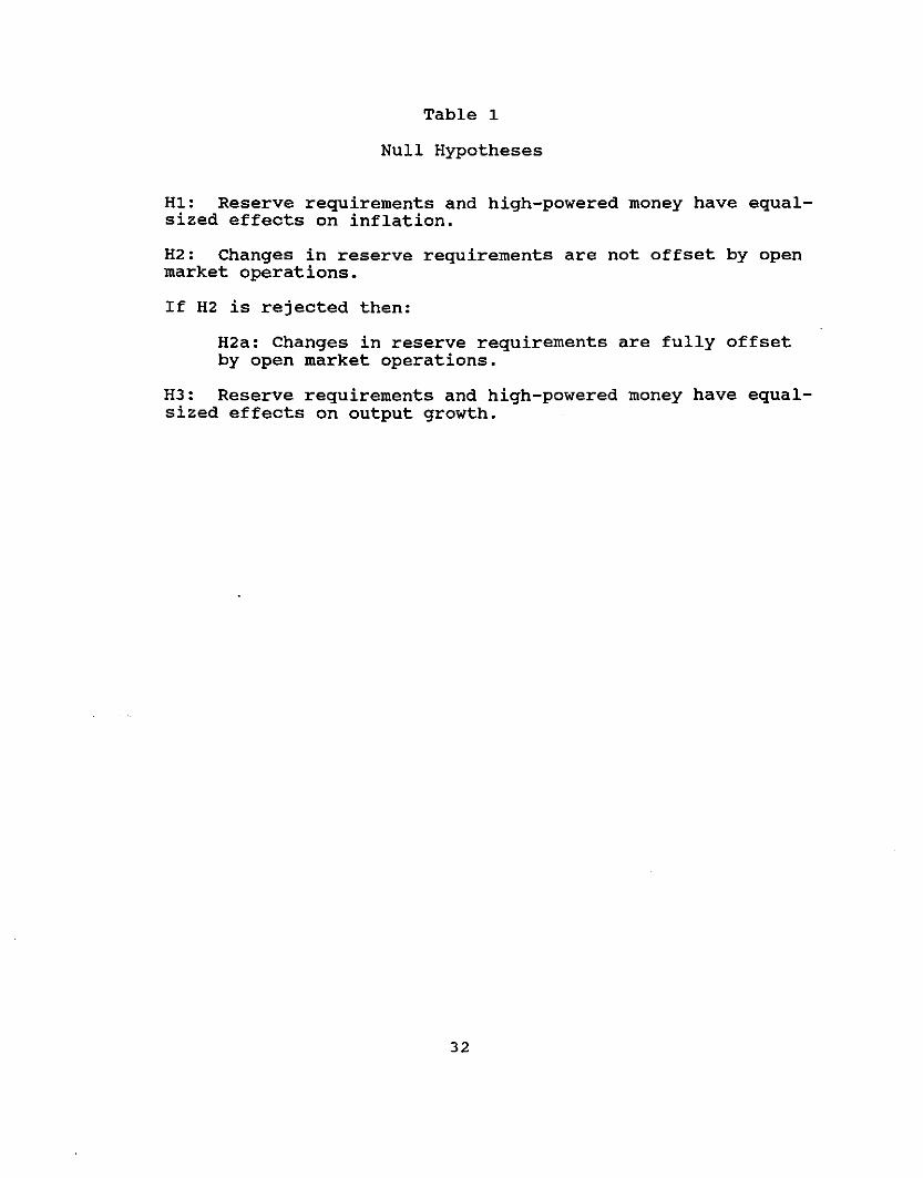
Table 1

Null Hypotheses

H1: Reserve requirements and high-powered money have equal­sized effects on inflation.

H2: Changes in reserve requirements are not offset by openmarket operations.

If H2 is rejected then:

H2a: Changes in reserve requirements are fully offsetby open market operations.

H3: Reserve requirements and high-powered money have equal­sized effects on output growth.

32

Table 2

Tests of Exclusion Restrictions

A A A A

Model [RSI< H< mm2< INF< GOP<]

A A A

Equation RSI H IlIllI2 INF GOPA

RSI 2.55** 0.68 0.75 2.61** 3.33**

A

H 4.77** 14.16** 2.55** 0.58 0.91

A

mm2 0.39 1.17 8.01** 2.23* 0.42

INF 0.68 1. 37 1.06 50.70** 2.45**

A

GOP 4.01*· 2.98** 4.62** 4.27** 0.56

* Indicates that the null hypothesis is rejected at the 10% level.

** Indicates that the null hypothesis is rejected at the 5% level.

33

Table 3

Control Model, 1959-90

(2) = -0.72"" RSI<(0.071)

- 0.509"" mm2<(0.081)

- 0.259 INF< +. z2<(0.21)

(3)

(4)

mm2< = 0.006 INF< + 0.878 GDP< + Z3<(0.459) (0.753)

INF< = 0.088 RSI< + 0.158" H< + z4<(0.082) (0.106)

(5) GDP< = -0.121 RSI< + 0.441 H<(0.323) (0.505)

0.758 mm2< + z5<(0.731)

----------------------------------------------------------------------Modified Sims Model 1948-91

(2) INV< = -0.003 RSI<(0.242)

+ 0.011" r< + e2<(0.002)

(3) r< = -0.429 RSI< + 0.247 H< + 0.014 mm1< + e3<(6.089) (3.424) (0.186)

(4)

(5)

H< = -0.685" RSI< - 0.001 r<(0.065) (0.001)

y< = 0.199" INV< + 0.003" r<(0.028) (0.001)

+ 0.083 y< + 0.271" P< + e4<(0.051) (0.095)

- 0.083 mm1< + e5<(0.170)

(6) P< = -0.034 RSI, + 0.001 r<(0.041) (0.001)

+ 0.017 Ht(0.018)

- 0.012 y< + e6<(0.043)

(7) U< = -1.147 INV< - 0.098" r<(0.935) (0.025)

- 16.161" y<( 2.332)

- 4.752 Pt + e7<(3.606)

(8) mm1 t = 0.001 r< + 0.140 Yt - 0.108 Pt + e8t(0.001) (0.130) (0.114)

34

Table 3 (cont.)

Supply-Shock Structural Model, 1959-90

(2) = -9.987 Pt + w2 t(27.397)

(3) = -0.54** RSIt

(0.089)- 0.336" mm2 t

(0.074)+ 0.162 Pt + w3 t

(0.25)

(4)

(5)

mm2 t = -0.022 RPEt(0.028)

Pt = -0.024 RSI t +(0.09)

0.168 Pt + w4 t(0.215)

0.157 RPEt + 0.079 Ht - 0.027 Yt + w5t(0.235) (0.091) (0.072)

(6) = 0.171 RSIt - 0.003 RPEt +(0.179) (0.06)

0.336" Ht + 0.295 mm2 t + W6t(0.167) (0.146)

Note: standard errors are in parentheses

35

Chart 1

Dynamic Response to a 1% Innovation in RSIControl Model

-- -.... - - ..

- . -~

'.

,-'"

(a) Inflation RatePercent Change

0.35

0.30

0.25

0.20

0.15

0.10 ,.- ........ 10%0.05 I "'-- - .................

I '-_0.00 -F=-""'_=-_=----,-----------.:.......----=-=-----_-::::-

-0.05 +--r---.---.-----r-.--.,....--r---.---.--,-----,.--..--r---.---.--,-----,.--~

o 1 2 3 4 5 6 7 8 9 10 11 12 13 14 15 16 17 18 19Step Ahead Forecast

(b) Output GrowthPercent Change

1.00

•0.80

\

0.60

-,

" 90%, '0.40

0.20

..- - .. - -- - -- - -- - -

0.00 1-~1:0%;;\-"--~/\~'====\~==~=:- -~-~._~.~-~- ~-~~~-==:===-=====:-=-:==--0.20 \ I \ __ -

v --, /---0.40 +--.---,----,-.---.--,.--,'+--.---,----,-,--.,----,--,----,-.---.--,.--.,

o 2 3 4 5 6 7 8 9 10 11 12 13 14 15 16 17 18 19Step Ahead Forecast

(a) Inflation RatePercent Change

0.35

Chart 2

Dynamic Response to a 1% Innovation in HControl Model

0.3 90%

.'0.25

0.2

0.15

01 / - --. ---...../ 10% ----.....

0.05..J --- ___

--- ---o¥---"r-~----------------:::::"-==-~

-0.05 -I---'-~-r------.-,..---r--,-~-r------.-,.---r---,-~-r------.-,.---r--,

o 1 2 3 4 5 6 7 8 9 10 11 12 13 14 15 16 17 18 19Step Ahead Forecast

••,

, '

,,.,

(b) Output GrowthPercent Growth

0.7

0.6

0.5

0.4

'.

'.90%

4 5 6 7 8 9 10 11 12 13 14 15 16 17 18 19Step Ahead Forecast

2 3

0.3

0.2

0.1o -k--co-----~=>,,.----:...--~~~--~-'-.-'-..:...;-:...;.:.=.• ..:.• ..:.--::....:...::....

.........-0.1 '\ /\ __--02 \ / \ - --

. 10% V\..-......... _ --0,3 '\. ,.,. -""'- -.-' - -

-0.4 +--.--___r-.__~-.-----,----,.__~-,-~~-~~~___r-.__~_.__~

o

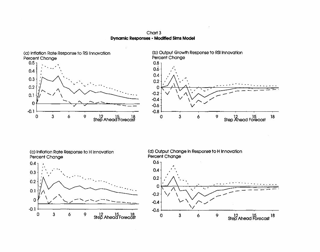
Chart 3Dynamic Responses - Modified Sims Model

•,

12 15 18Step Ahead Forecast

963

•,

(b) Output Growth Response to RSI InnovationPercent Change0.80.60.40.2

j.--.J \\ • _... --O~I 1\ ---.. ---.~ .. --

-0.2 VI \ V }~.. , '---' ~ .;::==::=:::>- - .-0.4-0.6-0.81--~-_----~--~---

o

0.3

0.2 1of \,

v~

...

O'~r...... / \

~ ------ . --....

"- ........ _--"- ;;I :.7 ------0.1

0 3 6 9 12 llj: 1~Step Ahead oreca

(a) Inflation Rate Response to RSllnnovationPercent Change

0.5

0.4

--

12 15 18Step Ahead Forecast

9

,...--

63

,

_ .... _--- .. _---0.2kI \ -'. ... '.' .~ _o I\~ '.

-0.2

-0.4 j \;-0.6

o

(d) Output Change in Response to H InnovationPercent Change

0.6

0.4

12 15 18Step AheaaForecaSt

... , ..

9

-.

6

'.

3

,. ~ ~, ,,

"-Of ',,/ '-.../- ..... "'--"'--- _

O. 111/\ . - - ~__________ '. -

0.3

0.2

(c) Inflation Rate Response to H InnovationPercent Change

0.4

-0.1 -1-1-------_-_-__-~o

Chart 4Dynamic Responses - Supply Shock Model

9 12 15 18Step Ahead Forecast

•, .I \. ~ ... ~

(b) Output growth response to RSI InnovationPercent Change0.8

,.0.6

0.4

0.2 / \

~r"A\~~:,'0:~~~~:~~~::-.L_~/C-__v'=-----=-_---:-=-_-;;_~_-0.4 Io 3 6

~ - .

12 15 18Step Ahead Forecast

-- .

96

/ . '

3

'.

(0) Inflotion rote responses to RSllnnovotionPercent Chonges0,30

0,25

0.20

0,15

0.10

0,050,00r.... '\ ' '\ ~-.....--- --~J __ ,

-0,05o

(c) Inflation Rote Change in Response to HPercent Change0,4

.---.-------

9 12 15 18Step Ahead Forecast

63

.I • ,.'

\ 1\ \ r-_- -----./ \ / \ "'-/

.; /

0.2

o

-0.2

0.4

(d) Output Growth Changes In Response to HPercent Change0.6

-0.4 +-1--~--~----~--~---o

- . -- - .

12 15 18Step Ahead Forecast

9

-_.--~.

6

",

3

/,0.3

0.2

'" - -0.11 I-.../ ./ ....... _

./01'-" .... j

-0.1 1o

Chart 5Dynamic Responses In Inflation Rates

Full Accomodation Experiment

(0) Control Model (b) Modified Sims ModelPercent Change Percent Change

0,25, 0,400,351

r • , ", '0.2 1 . . , .

, . .~ . , . 0.30.. . ,

0.151 . 0.25-.. 0.20 . \

."0,1 1 : / ~ , . . ~

~ - ...0.15 ....

/\0,051:1 ----- 0.10 ·r'..; \ V"/" I v ------ ...

Ok ," < ....... ,e ......

0,05 '-,}~, 0,00 f\ .....= .....-, ,-I ------ V '-/

=00::::: ____

-0,05 I -0.05a 3 6 9 lAh 15 18 a 3 6 9 ~ 15 18

Step ead Forecast Step ead Forecast

"

"~~ - ,

~ ..

\ /"--/ ,--/--'--- ---

3 6 9 12 15 18Step Ahead Forecast

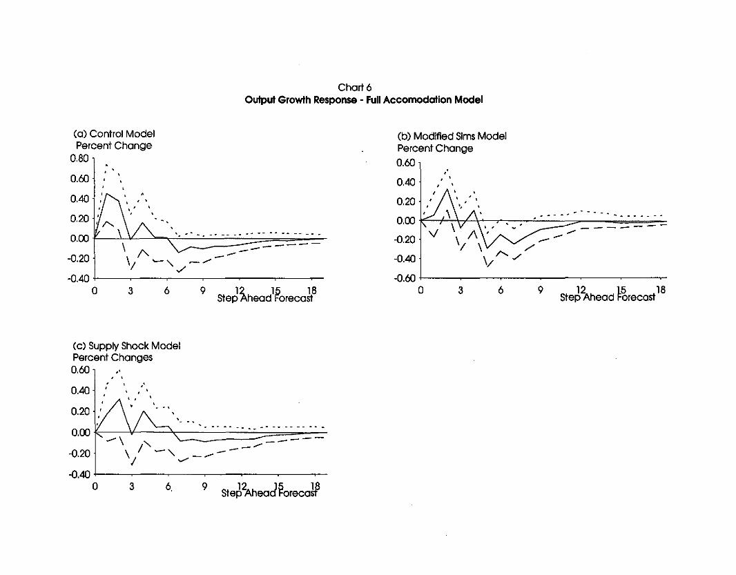
Chart 6output Growth Response - Full Accomodation Model

12 15 18Step Ahead Forecast

96

, ~ ............

3

,., .,

(b) Modified Sims ModelPercent Change0.60

0,40

0,20

0,00 .~/ \\/,\", , '. , • - -' - .• - .. - .-0,20 ,,~~ - .••....

-0,40 - --

-0.60 O~I-~~--;--~---::----~9 12 15 18

Step Ahead Forecast6

,, ,

3

(a) Control ModelPercent Change

0,80

0.60

0,40

0.20 f" \_::: \/; 0=-_ .... -~~~~. -~.-/ --, ~/---

-0,40 I ./,o '

(c) Supply Shock ModelPercent Changes0,60 1 .',

Ste~2Ahead~orecaMl96.3

.•0.40

0,20

\/~'-"'-""-"--''''''''''0.00 ; ~ .----\ '- --

/..... _......

-0.20 '; - '\, ...... --

-0.40-I------------~-~-o

RESEARCH PAPERS OF THE RESEARCH DEPARTMENTFEDERAL RESERVE BANK OF DALLAS

Available, at no charge, from the Research DepartmentFederal Reserve Bank of Dallas, Station K

Dallas, Texas 75222

9201 Are Deep Recessions Followed by Strong Recoveries? (Mark A. Wynne andNathan S. Balke)

9202 The Case of the "Missing M2" (John V. Duca)

9203 Immigrant Links to the Home Country: Implications for Trade, Welfare andFactor Rewards (David M. Gould)

9204 Does Aggregate Output Have a Unit Root? (Mark A. Wynne)

9205 Inflation and Its Variability: A Note (Kenneth M. Emery)

9206 Budget Constrained Frontier Measures of Fiscal Equality and Efficiency inSchooling (Shawna Grosskopf, Kathy Hayes, Lori Taylor, William Weber)

9207 The Effects of Credit Availability, Nonbank Competition, and Tax Reform onBank Consumer Lending (John V. Duca and Bonnie Garrett)

9208 On the Future Erosion of the North American Free Trade Agreement (William C.Gruben)

9209 Threshold Cointegration (Nathan S. Balke and Thomas B. Fomby)

9210 Cointegration and Tests of a Classical Model of Inflation in Argentina, Bolivia,Brazil, Mexico, and Peru (Raul Anibal Feliz and John H. Welch)

9211 Nominal Feedback Rules for Monetary Policy: Some Comments (Evan F.Koenig)

9212 The Analysis of Fiscal Policy in Neoclassical Models' (Mark Wynne)

9213 Measuring the Value of School Quality (Lori Taylor)

9214 Forecasting Turning Points: Is a Two-State Characterization of the BusinessCycle Appropriate? (Kenneth M. Emery & Evan F. Koenig)

9215 Energy Security: A Comparison of Protectionist Policies (Mine K. YOcel andCarol Dahl)

9216 An Analysis of the Impact of Two Fiscal Policies on the Behavior of aDynamic Asset Market (Gregory W. Huffman)

9301 Human Capital Externalities, Trade, and Economic Growth(David Gould and Roy J. Ruffin)

9302 The New Face of Latin America: Financial Flows, Markets, and Institutions in the1990s (John Welch)

9303 A General Two Sector Model of Endogenous Growth with Human andPhysical Capital (Eric Bond, Ping Wang, and Chong K. Yip)

9304 The Political Economy of School Reform (S. Grosskopf, K. Hayes, L. Taylor,and W. Weber)

9305 Money, Output, and Income Velocity (Theodore Palivos and Ping Wang)

9306 Constructing an Alternative Measure of Changes in Reserve RequirementRatios (Joseph H. Haslag and Scott E. Hein)

9307 Money Demand and Relative Prices During Episodes of Hyperinflation(Ellis W. Tallman and Ping Wang)

9308 On Quantity Theory Restrictions and the Signalling Value of the Money Multiplier(Joseph Haslag)

9309 The Algebra of Price Stability (Nathan S. Balke and Kenneth M. Emery)

9310 Does It Matter How Monetary Policy is Implemented? (Joseph H. Haslag andScott E. Hein)