feature extraction and dimension reduction with
TRANSCRIPT

Feature Extraction and Dimension Reduction
with Applications to Classification
and the Analysis of Co-occurrence Data
a dissertation
submitted to the department of statistics
and the committee on graduate studies
of stanford university
in partial fulfillment of the requirements
for the degree of
doctor of philosophy
Mu Zhu
June 2001

c© Copyright by Mu Zhu 2001
All Rights Reserved
ii

I certify that I have read this dissertation and that in my
opinion it is fully adequate, in scope and quality, as a disser-
tation for the degree of Doctor of Philosophy.
Trevor J. Hastie(Principal Advisor)
I certify that I have read this dissertation and that in my
opinion it is fully adequate, in scope and quality, as a disser-
tation for the degree of Doctor of Philosophy.
Jerome H. Friedman
I certify that I have read this dissertation and that in my
opinion it is fully adequate, in scope and quality, as a disser-
tation for the degree of Doctor of Philosophy.
Robert J. Tibshirani
Approved for the University Committee on Graduate Studies:
iii
Abstract
The Internet has spawned a renewed interest in the analysis of co-occurrence data. Cor-
respondence analysis can be applied to such data to yield useful information. A less well-
known technique called canonical correspondence analysis (CCA) is suitable when such data
come with covariates. We show that CCA is equivalent to a classification technique known
as linear discriminant analysis (LDA). Both CCA and LDA are examples of a general fea-
ture extraction problem.
LDA as a feature extraction technique, however, is restrictive: it can not pick up high-
order features in the data. We propose a much more general method, of which LDA is a
special case. Our method does not assume the density functions of each class to belong to
any parametric family. We then compare our method in the QDA (quadratic discriminant
analysis) setting with a competitor, known as the sliced average variance estimator (SAVE).
Our study shows that SAVE over-emphasizes second-order differences among classes.
Our approach to feature extraction is exploratory and has applications in dimension re-
duction, automatic exploratory data analysis, and data visualization. We also investigate
strategies to incorporate the exploratory feature extraction component into formal proba-
bilistic models. In particular, we study the problem of reduced-rank non-parametric dis-
criminant analysis by combining our work in feature extraction with projection pursuit
density estimation. In the process, we uncover an important difference between the forward
and backward projection pursuit algorithms, previously thought to be equivalent.
iv

Finally, we study related mixture models for classification and show there is a direct con-
nection between a particular formulation of the mixture model and a popular model for
analyzing co-occurrence data known as the aspect model.
v

Acknowledgments
Microsoft’s Bill Gates and Yahoo’s Jerry Yang are perhaps two of the most celebrated icons
in our new economy. Bill Gates and I went to the same college: I got my degree; he didn’t.
Jerry Yang and I went to the same graduate school: I am about to finish my degree; he still
hasn’t. People say it is much better to be a drop-out these days: Only those drop-outs go
on to make their millions, while those who stay behind will have to prepare to live a very
humble life.
At a time like this, I must thank those who have supported me as I choose to go on
the less popular (and much less financially-rewarding) path of personal intellectual satis-
faction. These include my parents and sister. When I went to college, there were only
two students directly admitted from China. The other, much smarter than I am, has gone
back to China and started his Internet business. Now living his life as a business executive
under the spot light, he has become a cultural phenomenon that has inspired a whole new
generation in China to regard MBA as the ultimate Holy Grail in one’s academic career.
Under such social influences, it must be very difficult for any parents to support what I chose
to do. I owe them a great deal for their understanding and feel extremely grateful and proud.
In the same regard, I am also lucky to have a supporting wife. We have shared similar
values, and have not had to defend our personal convictions in front of one another. This
is a blessing, especially for those who respect the value of a tranquil and satisfying personal
inner-life.
vi

For someone who so highly values intellectual satisfaction, I am very lucky to have cho-
sen Professor Trevor Hastie as my mentor. He gave me the exact kind of guidance that
I need and feel comfortable with. I am a very independent person. If I were asked to
work on a problem, 99% of the time I would end up hating it. Trevor did not force me
to work on a particular problem, nor did he force me to work in a certain way. As his
student, I have the freedom to wander in the magical kingdom of science and enjoy myself.
The kingdom of science is so vast that a novice like me will occasionally get lost. When
this happened, Trevor pointed me in the right directions. They were not the directions
that would lead to a known destination, however, for this would have spoiled all the fun.
Instead, they were directions that would allow me to continue a journey of my own. As
a result, my career as a graduate student has turned out to be most fulfilling and rewarding.
I’ve also had the privilege to receive the same kind of guidance on occasion from professors
such as Rob Tibshirani, Jerry Friedman and Brad Efron. Together with Trevor, they have
also influenced me a great deal through their own life-time work. For the opportunity to
study with these incredible professors, I owe the most to Professor Jun S. Liu — I would
never have chosen to study statistics or come to Stanford had I not met Jun when I was an
undergraduate.
Finally, I’d like to thank Helen Tombropoulos for proof-reading my manuscript, and for
the fine example that she has set as a very strong and perpetually optimistic person.
Mu Zhu
Stanford, California
June 2001
vii

Preface
This preface is primarily meant to be a reading guide for the committee members. It gives
detailed section and page numbers pointing to the most important contributions in this
thesis. Other readers should go directly to Chapter 1.
For enhanced readability, every chapter begins with a brief outline, except for chapter
1, which is an introductory chapter in itself. These short outlines contain the main flow of
ideas in this thesis, and state the main contributions from each chapter. The main chapters
— those that contain new methodological contributions — are chapters 2, 4, 5 and 6. A
detailed break-down of the chapters is as follows:
Chapter 1 is an introduction. We start with the analysis of co-occurrence data and re-
lated applications (example 1, p. 2; example 2, p. 4). In section 1.4 (p. 8), we introduce
the problem of analyzing co-occurrence data with covariates (examples 3 and 4, p. 8). The
general problem of feature extraction is then introduced in section 1.5 (p. 10) and its im-
portance explained in section 1.6 (p. 11).
Chapter 2 is devoted to establishing the equivalence between linear discriminant analy-
sis (LDA), a well-known classification technique with a feature extraction component, and
canonical correspondence analysis (CCA), a common method for analyzing co-occurrence
data with covariates. We first review the two techniques. The equivalence is shown in
section 2.3 (p. 20-26), both algebraically and model-wise. In sections 2.4 and 2.5 (p. 26-29),
we point out the fundamental limitations of LDA (and hence CCA) — that it cannot pick
up high-order features in the data — and motivate the need for a generalization.
viii

Chapter 3 is a review of various classification techniques. The most important section
is section 3.2.5 (p. 39), where we point out how the materials of this thesis fit into the
statistical literature of classification.
In chapter 4, we develop a general technique for identifying important features for clas-
sification. The main method and the basic heuristics for its implementation are given in
sections 4.3 and 4.4 (p. 44-50). Sections 4.6.3 (p. 53) and 4.7 (p. 55-61) describe two useful
and practical strategies for finding multiple features, one by orthogonalization and another
by feature removal.
In chapter 5, we specialize our general approach developed in chapter 4 to the case of
quadratic discriminant analysis (QDA) and compare our method with a competitor: the
sliced average variance estimator (SAVE). The most important conclusion is that SAVE
over-emphasizes second-order information (section 5.3, p. 73-77; section 5.4.3, p. 85 and
section 5.4.4, p. 86).
In chapter 6, we combine our general feature extraction technique with projection pursuit
density estimation (PPDE) to produce a general model for (reduced-rank) non-parametric
discriminant analysis (section 6.2, p. 101-103). In section 6.1 (p. 90-101), we review PPDE
and uncover an important difference between the forward and backward projection pursuit
algorithms, previously thought to be equivalent. This difference has significant consequences
when one considers using the projection pursuit paradigm for non-parametric discriminant
analysis (section 6.2.2, p. 106-108).
In the last chapter, chapter 7, we review some related mixture models for discriminant
analysis (MDA). The main contribution of this chapter is in section 7.6 (p. 124), where we
point out a direct connection between a certain variation of MDA and a natural extension of
Hofmann’s aspect model for analyzing co-occurrence data with covariates. A brief summary
of the entire thesis is then given in section 7.7 (p. 125).
ix

Contents
Abstract iv
Acknowledgments vi
Preface viii
1 Introduction 1
1.1 Co-occurrence Data . . . . . . . . . . . . . . . . . . . . . . . . . . . . . . . 1
1.2 Correspondence Analysis and Ordination . . . . . . . . . . . . . . . . . . . 3
1.3 Aspect Model . . . . . . . . . . . . . . . . . . . . . . . . . . . . . . . . . . . 7
1.4 Co-occurrence Data with Covariates and Constrained Ordination . . . . . . 8
1.5 The General Problem of Feature Extraction . . . . . . . . . . . . . . . . . . 10
1.6 The Significance of Feature Extraction . . . . . . . . . . . . . . . . . . . . . 11
1.7 Organization . . . . . . . . . . . . . . . . . . . . . . . . . . . . . . . . . . . 13
2 Co-occurrence Data and Discriminant Analysis 15
2.1 Correspondence Analysis with Covariates . . . . . . . . . . . . . . . . . . . 15
2.2 Linear Discriminant Analysis (LDA) . . . . . . . . . . . . . . . . . . . . . . 17
2.2.1 Gaussian Discrimination . . . . . . . . . . . . . . . . . . . . . . . . . 17
2.2.2 Linear Discriminant Directions . . . . . . . . . . . . . . . . . . . . . 18
2.2.3 Connections . . . . . . . . . . . . . . . . . . . . . . . . . . . . . . . . 19
2.3 Equivalence Between CCA and LDA . . . . . . . . . . . . . . . . . . . . . . 20
2.3.1 Algebra for LDA . . . . . . . . . . . . . . . . . . . . . . . . . . . . . 21
2.3.2 Algebra for CCA . . . . . . . . . . . . . . . . . . . . . . . . . . . . . 23
x
2.3.3 Algebraic Equivalence . . . . . . . . . . . . . . . . . . . . . . . . . . 24
2.3.4 Model Equivalence . . . . . . . . . . . . . . . . . . . . . . . . . . . . 25
2.4 Flexible Response Curves and Flexible Class Densities . . . . . . . . . . . . 26
2.5 The Limitations of LDA . . . . . . . . . . . . . . . . . . . . . . . . . . . . . 28
2.6 Summary . . . . . . . . . . . . . . . . . . . . . . . . . . . . . . . . . . . . . 29
3 Classification 30
3.1 Modeling Posterior Probabilities . . . . . . . . . . . . . . . . . . . . . . . . 31
3.1.1 Logistic Regression . . . . . . . . . . . . . . . . . . . . . . . . . . . . 31
3.1.2 Generalized Additive Models (GAM) . . . . . . . . . . . . . . . . . . 32
3.1.3 Projection Pursuit Logistic Regression . . . . . . . . . . . . . . . . . 33
3.2 Modeling Class Densities . . . . . . . . . . . . . . . . . . . . . . . . . . . . . 33
3.2.1 Gaussian Discrimination . . . . . . . . . . . . . . . . . . . . . . . . . 34
3.2.2 Regularization . . . . . . . . . . . . . . . . . . . . . . . . . . . . . . 35
3.2.3 Flexible Decision Boundaries . . . . . . . . . . . . . . . . . . . . . . 36
3.2.4 Non-Parametric Discrimination . . . . . . . . . . . . . . . . . . . . . 38
3.2.5 Theoretical Motivation of the Thesis . . . . . . . . . . . . . . . . . . 39
3.3 Connections . . . . . . . . . . . . . . . . . . . . . . . . . . . . . . . . . . . . 39
3.4 Other Popular Classifiers . . . . . . . . . . . . . . . . . . . . . . . . . . . . 40
4 A General Methodology for Feature Extraction 42
4.1 Data Compression . . . . . . . . . . . . . . . . . . . . . . . . . . . . . . . . 42
4.2 Variable Selection . . . . . . . . . . . . . . . . . . . . . . . . . . . . . . . . . 43
4.3 Feature Extraction . . . . . . . . . . . . . . . . . . . . . . . . . . . . . . . . 44
4.4 Numerical Optimization . . . . . . . . . . . . . . . . . . . . . . . . . . . . . 48
4.5 Illustration . . . . . . . . . . . . . . . . . . . . . . . . . . . . . . . . . . . . 50
4.6 Finding Multiple Features . . . . . . . . . . . . . . . . . . . . . . . . . . . . 51
4.6.1 Optimal Discriminant Subspaces . . . . . . . . . . . . . . . . . . . . 52
4.6.2 Sequence of Nested Discriminant Subspaces . . . . . . . . . . . . . . 53
4.6.3 Orthogonal Features . . . . . . . . . . . . . . . . . . . . . . . . . . . 53
4.7 Non-orthogonal Features . . . . . . . . . . . . . . . . . . . . . . . . . . . . . 55
4.7.1 Exploratory Projection Pursuit . . . . . . . . . . . . . . . . . . . . . 56
xi

4.7.2 Finding Non-orthogonal Features via Feature Removal . . . . . . . . 58
4.8 Examples . . . . . . . . . . . . . . . . . . . . . . . . . . . . . . . . . . . . . 61
5 Feature Extraction in the Gaussian Family 68
5.1 Feature Extraction for QDA . . . . . . . . . . . . . . . . . . . . . . . . . . . 69
5.1.1 LR(α) When pk = N(µk,Σk) . . . . . . . . . . . . . . . . . . . . . . 69
5.1.2 Data Standardization . . . . . . . . . . . . . . . . . . . . . . . . . . 70
5.2 Sliced Average Variance Estimator (SAVE) . . . . . . . . . . . . . . . . . . 72
5.3 Comparison . . . . . . . . . . . . . . . . . . . . . . . . . . . . . . . . . . . . 73
5.3.1 A Numerical Example . . . . . . . . . . . . . . . . . . . . . . . . . . 74
5.3.2 Order of Discriminant Directions . . . . . . . . . . . . . . . . . . . . 77
5.3.3 SAVE(α) vs. LR(α) . . . . . . . . . . . . . . . . . . . . . . . . . . . 77
5.4 Feature Extraction with Common Principal Components . . . . . . . . . . . 80
5.4.1 Uniform Dissimilarity . . . . . . . . . . . . . . . . . . . . . . . . . . 80
5.4.2 Special Algorithm . . . . . . . . . . . . . . . . . . . . . . . . . . . . 84
5.4.3 SAVE(α) vs. LR(α): An Experiment . . . . . . . . . . . . . . . . . . 85
5.4.4 Example: Pen Digit Data . . . . . . . . . . . . . . . . . . . . . . . . 86
5.5 Conclusion . . . . . . . . . . . . . . . . . . . . . . . . . . . . . . . . . . . . 87
6 Reduced-Rank Non-Parametric Discrimination 89
6.1 Projection Pursuit Density Estimation . . . . . . . . . . . . . . . . . . . . . 90
6.1.1 Forward Algorithm . . . . . . . . . . . . . . . . . . . . . . . . . . . . 91
6.1.2 Backward Algorithm and Its Difficulties . . . . . . . . . . . . . . . . 92
6.1.3 A Practical Backward Algorithm . . . . . . . . . . . . . . . . . . . . 94
6.1.4 Non-equivalence Between the Forward and Backward Algorithms . . 94
6.1.5 Projection Pursuit and Independent Component Analysis . . . . . . 100
6.2 Regularized Non-Parametric Discrimination . . . . . . . . . . . . . . . . . . 101
6.2.1 Forward Algorithm . . . . . . . . . . . . . . . . . . . . . . . . . . . . 103
6.2.2 Backward Algorithm . . . . . . . . . . . . . . . . . . . . . . . . . . . 106
6.3 Illustration: Exclusive Or . . . . . . . . . . . . . . . . . . . . . . . . . . . . 108
xii

7 Mixture Models 113
7.1 Mixture Discriminant Analysis (MDA) . . . . . . . . . . . . . . . . . . . . . 114
7.2 LDA as a Prototype Method . . . . . . . . . . . . . . . . . . . . . . . . . . 115
7.3 K-means vs. Learning Vector Quantization (LVQ) . . . . . . . . . . . . . . 115
7.3.1 Separate K-means . . . . . . . . . . . . . . . . . . . . . . . . . . . . 115
7.3.2 Learning Vector Quantization (LVQ) . . . . . . . . . . . . . . . . . . 116
7.4 Extensions of MDA . . . . . . . . . . . . . . . . . . . . . . . . . . . . . . . . 118
7.4.1 Shrinking Centroids . . . . . . . . . . . . . . . . . . . . . . . . . . . 118
7.4.2 Competing Centroids . . . . . . . . . . . . . . . . . . . . . . . . . . 118
7.5 Illustrations . . . . . . . . . . . . . . . . . . . . . . . . . . . . . . . . . . . . 120
7.6 Aspect Model with Covariates . . . . . . . . . . . . . . . . . . . . . . . . . . 124
7.7 Summary . . . . . . . . . . . . . . . . . . . . . . . . . . . . . . . . . . . . . 125
A Eigenvalue Problems 126
A.1 The Basic Eigenvalue Problem . . . . . . . . . . . . . . . . . . . . . . . . . 126
A.2 The Generalized Eigenvalue Problem . . . . . . . . . . . . . . . . . . . . . . 127
A.3 Principal Components . . . . . . . . . . . . . . . . . . . . . . . . . . . . . . 128
A.4 Linear Discriminant Analysis . . . . . . . . . . . . . . . . . . . . . . . . . . 128
B Numerical Optimization 129
B.1 The Generic Optimization Algorithm . . . . . . . . . . . . . . . . . . . . . . 129
B.2 Choice of Descent Direction . . . . . . . . . . . . . . . . . . . . . . . . . . . 130
B.2.1 Steepest Descent . . . . . . . . . . . . . . . . . . . . . . . . . . . . . 130
B.2.2 Newton’s Method . . . . . . . . . . . . . . . . . . . . . . . . . . . . . 130
B.3 Choice of Step Size . . . . . . . . . . . . . . . . . . . . . . . . . . . . . . . . 131
C Density Estimation 132
C.1 Kernel Density Estimation . . . . . . . . . . . . . . . . . . . . . . . . . . . . 132
C.2 The Locfit Package in Splus . . . . . . . . . . . . . . . . . . . . . . . . . . 133
Bibliography 134
xiii

Chapter 1
Introduction
In e-commerce applications, a particular type of data structure called co-occurrence data
(or transposable data as coined by professor Art Owen of Stanford University) arises quite
often. Due to the fast-growing e-commerce market, researchers in data-mining and artificial
intelligence, as well as statistics, have spawned a renewed interest in analyzing datasets of
this form, especially on a large scale.
1.1 Co-occurrence Data
Co-occurrence data come in the form of a matrix, Y , whose entry yik ≥ 0 is an indicator or
a frequency count of the co-occurrence of two (categorical) variables ξi ∈ X = ξ1, ξ2, ..., ξIand ηk ∈ Y = η1, η2, ..., ηK. A generic co-occurrence matrix is illustrated in table 1.1.
η1 ... ηK
ξ1 y11 ... y1K
ξ2 y21 ... y2K...
.... . .
...ξI yI1 ... yIK
Table 1.1: A generic co-occurrence matrix Y . Each entry yik can be a binary indicator ora frequency count of the event that ηk and ξi has co-occurred.
Data arranged in this format are usually known in classical statistics as contingency tables.
1

CHAPTER 1. INTRODUCTION 2
They occur in a wide range of real applications. Various classical methods, such as log-
linear models, exist for analyzing data of this form. The Internet has revived a tremendous
amount interest in the techniques for analyzing this type of data on a much larger scale.
Here is a real example from a Silicon Valley start-up.
Example 1 (Personalization) Most commercial web-pages contain a number of adver-
tising items. These sites usually have a large database of possible products to advertise,
but can show you only a few on each web-page. Therefore every time you visit a web-page,
a few such items are selected and displayed. In some cases, the selection is random. In
Customer Item 1 Item 2 ... Item 10
1 3 4 ... 22 5 4 ... 43 4 4 ... 3...
......
. . ....
35 4 3 ... 536 4 3 ... 437 2 1 ... 3
Table 1.2: Real consumer preference data from a pilot test project conducted by an Internetcompany in the Silicon Valley.
other cases, especially when you log on using an existing personal account, the host site
would know something about you already (e.g., from your past transaction records) and
would actually try to select items that would most likely cater to your individual tastes and
catch your attention in order to increase their sales. This process is known in the industry
as personalization. They can do this by analyzing (mining) their customer database. Table
1.2 shows an example of one such database. It is a co-occurrence matrix, with
X = ξi = Customer 1, Customer 2, ..., Customer 37
and
Y = ηk = Item 1, Item 2, ..., Item 10.
In this case, 37 customers were asked to rate 10 different products using a 1-5 scale. More

CHAPTER 1. INTRODUCTION 3
often than not, such explicit ratings are not available. Instead, these will be binary indi-
cators (e.g., whether a customer has purchased this item before) or frequency counts (e.g.,
the number of times a customer have clicked on this item in the past), which can still be
interpreted as measures of consumer preferences.
1.2 Correspondence Analysis and Ordination
A classic statistical problem for contingency tables is known as ordination. The goal of
ordination is to put the categories ξi and ηk into a logical order. To achieve this goal,
we seek to find a score for each row category ξi and a score for each column category ηk
simultaneously. Let zi and uk be these scores. The categories can then be ordered using
these scores: items with similar scores are more likely to occur (co-occur) together. Suppose
that we know all the uk’s, then we should be able to calculate the zi’s by a simple weighted
average (see below), and vice versa. Therefore,
zi =
∑Kk=1 yikuk∑K
k=1 yik
and uk =
∑Ii=1 yikzi∑I
i=1 yik
.
It is well-known that the solution for the reciprocal averaging equations above can be ob-
tained from a simple eigen-analysis (see [23]). In matrix notation, we can write the above
equations as
z ∝ A−1Y u and u ∝ B−1Y T z,
where A = diag(yi·) with yi· =∑K
k=1 yik, and B = diag(y·k) with y·k =∑I
i=1 yik. Thus, we
have
z ∝ A−1Y B−1Y T z and u ∝ B−1Y T A−1Y u
suggesting that z and u are eigenvectors of A−1Y B−1Y T and B−1Y T A−1Y , respectively.
However, the eigenvectors corresponding to the largest eigenvalue of 1 is a trivial vector
of one’s, i.e., 1 = (1, 1, ..., 1)T . Hence one identifies the eigenvectors corresponding to the
next largest eigenvalue as the best solution. For more details, see [30], p. 237-239, and [17],

CHAPTER 1. INTRODUCTION 4
section 4.2. This technique is known as correspondence analysis. The scores zi and uk are
scores on a (latent) ordination axis, a direction in which the items can be ordered.
One way to find these eigenvectors is by iteration, outlined in algorithm 1.1. The essence
Algorithm 1.1 Iterative Correspondence Analysis
1. Start with an arbitrary initial vector z = z0 6= 1, properly standardized, so that
I∑
i=1
yi·zi = 0 and
I∑
i=1
yi·z2i = 1.
Note since 1 is an eigenvector itself, starting with 1 will cause the iteration to “stall”at the trivial solution.
2. Let z = A−1Y u.
3. Let u = B−1Y T z and standardize z.
4. Alternate between steps (2) and (3) until convergence.
of this iteration procedure is the well-known power method to find the solutions to the
eigen-equations above. For more details, see [19], p. 197-198.
Example 2 (Ecological Ordination and Gaussian Response Model) In the ecolog-
ical ordination problem, Y = yik is a matrix whose element measures the abundance of
species k at site i. Naturally, some species are more abundant at certain locations than
others. There are reasons to believe that the key factor that drives the relative abundance
of different species is the different environment at these locations. The ordination problem
is to identify scores that rate the sites and species on the same (environmental) scale, often
called the environmental gradient in this context, or simply the ordination axis in general.
Sites that receive similar scores on the environmental gradient are similar in their envi-
ronmental conditions; species that receive similar scores on the environmental gradient are
similar in terms of their biological demand on environmental resources.
Correspondence analysis can be used to compute these scores. For many years, ecologists

CHAPTER 1. INTRODUCTION 5
have been interested in the simple Gaussian response model, which describes the relation-
ship between environment and species. Let zi be the environmental score that site i receives
and uk be the optimal environmental score for species k. Then the Gaussian response model
(see [37]) says that
yik ∼ Poisson(λik),
where λik depends on the scores zi and uk through
log λik = ak −(zi − uk)
2
2t2k.
The parameter tk is called the tolerance of species k. So the rate of occurrence of species
k at site i is described by a Gaussian curve that peaks when site i receives a score on the
environmental gradient that is optimal for species k, namely uk. Figure 1.1 provides an
illustration of this model.
site 1 site 2 site 3 site 4 site 5
species 1 species 2
Figure 1.1: Illustration of the Gaussian response model in the context of ecological ordina-tion. This graph depicts a situation where the (environmental) conditions at site 2 are closeto optimal for species 1, whereas site 3 is close to optimal for species 2.

CHAPTER 1. INTRODUCTION 6
Under the Poisson model, the maximum likelihood equations for zi and uk can be easily
obtained and are given by
zi =
∑Kk=1(yikuk)/t
2k
∑Kk=1 yik/t
2k
−∑K
k=1(zi − uk)λik/t2k
∑Kk=1 yik/t
2k
and
uk =
∑Ii=1 yikzi∑I
i=1 yik
−∑I
i=1(zi − uk)λik∑I
i=1 yik
.
In [37], it is argued that under certain conditions, the leading term in the maximum likeli-
hood equations dominates, whereby the equations can simply be approximated by
zi =
∑Kk=1(yikuk)/t
2k
∑Kk=1 yik/t
2k
and uk =
∑Ii=1 yikzi∑I
i=1 yik
.
If a further simplifying assumption is made — namely, all species have the same tolerance
level, or tk = t = 1 — then these equations reduce exactly to the reciprocal averaging
equations of correspondence analysis.
Although originated in the ecological research community, the Gaussian response model can
be viewed as a general probabilistic model for co-occurrence data. Instead of a single latent
score, each category ηk can be thought to have a response curve fk on a latent scale. The
probability of co-occurrence between ηk and ξi will be high if fk peaks at or close to xi, the
score for category ξi on the same latent scale.
Clearly, there are different ways of scoring (and ordering) the ξi’s and ηk’s. In fact, the
successive eigenvectors of A−1Y B−1Y T and B−1Y T A−1Y also lead to particular orderings
of the ξi’s and ηk’s, respectively, each on an ordination axis that is orthogonal to those
previously given. Hence a plot of these scores on the first two ordination axes, known as a
bi-plot, gives us a 2-dimensional view of the relationship among the ξi’s and ηk’s. There are
different scalings one could use to create a bi-plot, which lead to different ways the bi-plot
should be interpreted. It is, however, not directly related to our discussion here, and we
simply refer the readers to [30] for more details.

CHAPTER 1. INTRODUCTION 7
Example 1 (Personalization — Continued) The concept of ordination can be readily
applied to the personalization problem described in example 1. Figure 1.2 is a bi-plot of the
consumer preference data in table 1.2 as a result of correspondence analysis. We can see
Low-Dimensional RepresentationReal Test Data
Scale 1
Sca
le 2
1
2
3
4
5
6
7
8
9
10
1
2
3
4
5
6
7
8
9
10
11
12 1314
15
16
17
18
19
20
21
22
23
2425
26 27
28
2930
31
32
33
34
35
36
37
Figure 1.2: Real test data from a pilot study conducted by a Silicon Valley start-up, where 37customers were asked to rate 10 products. Circled numbers are products; un-circled numbersare customers. Shown here is a 2-dimensional representation of the relative position of thesecustomers and the products.
that products 2, 3, 4, 10 are close together and are, therefore, similar in the sense that they
tend to attract the same group of customers. Likewise, products 5 and 8 are far apart and,
therefore, probably appeal to very different types of customers. Hence if your past record
shows that you have had some interest in product 2, then you are likely to have an interest
in products 3, 4, and 10 as well.
1.3 Aspect Model
Instead of assigning scores to the categories, one can model the probabilities of co-occurrence
directly. One such model is the aspect model (see [24]), which is based on partitioning the
space of X × Y into disjoint regions indexed by several latent classes, cα = c1, c2, ..., cJ.Conditional on the latent class, the occurrence probabilities of ξi and ηk are modeled as
CHAPTER 1. INTRODUCTION 8
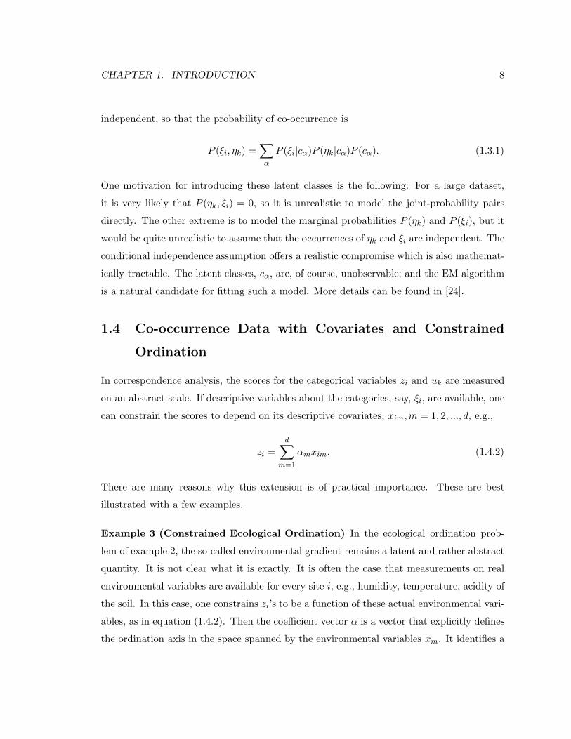
independent, so that the probability of co-occurrence is
P (ξi, ηk) =∑
α
P (ξi|cα)P (ηk|cα)P (cα). (1.3.1)
One motivation for introducing these latent classes is the following: For a large dataset,
it is very likely that P (ηk, ξi) = 0, so it is unrealistic to model the joint-probability pairs
directly. The other extreme is to model the marginal probabilities P (ηk) and P (ξi), but it
would be quite unrealistic to assume that the occurrences of ηk and ξi are independent. The
conditional independence assumption offers a realistic compromise which is also mathemat-
ically tractable. The latent classes, cα, are, of course, unobservable; and the EM algorithm
is a natural candidate for fitting such a model. More details can be found in [24].
1.4 Co-occurrence Data with Covariates and Constrained
Ordination
In correspondence analysis, the scores for the categorical variables zi and uk are measured
on an abstract scale. If descriptive variables about the categories, say, ξi, are available, one
can constrain the scores to depend on its descriptive covariates, xim,m = 1, 2, ..., d, e.g.,
zi =
d∑
m=1
αmxim. (1.4.2)
There are many reasons why this extension is of practical importance. These are best
illustrated with a few examples.
Example 3 (Constrained Ecological Ordination) In the ecological ordination prob-
lem of example 2, the so-called environmental gradient remains a latent and rather abstract
quantity. It is not clear what it is exactly. It is often the case that measurements on real
environmental variables are available for every site i, e.g., humidity, temperature, acidity of
the soil. In this case, one constrains zi’s to be a function of these actual environmental vari-
ables, as in equation (1.4.2). Then the coefficient vector α is a vector that explicitly defines
the ordination axis in the space spanned by the environmental variables xm. It identifies a

CHAPTER 1. INTRODUCTION 9
direction in which the demands on environmental resources are the most different between
different species. This problem is known as constrained ordination.
Example 4 (Targeted Marketing) Table 1.3 provides an illustration of a typical sce-
nario in a marketing study. The left side of the table is a co-occurrence matrix, much like in
example 1. The right side of the table contains some covariates for each shopper. One can
Shopper Games Wine Flowers Age Income Gender
1 1 0 0 21 $10K M2 1 1 0 59 $65K F3 0 1 1 31 $45K M
Table 1.3: Illustration of a typical scenario in a targeted marketing study. The left side of thetable is a co-occurrence matrix. The right side of the table contains descriptive informationabout each shopper that can be used to come up with useful prediction rules for targetedmarketing.
apply correspondence analysis to find the scores for each shopper and product. Based on
the scores, we can conclude that products whose scores are close tend to be bought together
and, similarly, shoppers whose scores are close are similar in their purchasing patterns.
Now suppose there comes a new customer. A very important question in targeted mar-
keting is to ask if we can identify a subset of the products that this customer may be
particularly interested in. Here, the scores we computed from correspondence analysis do
not help us, because we don’t know how to assign a new score to a new observation.
The aspect model suffers from a similar problem. One can certainly fit an aspect model for
the co-occurrence matrix on the left side. But given a new customer in X , we can’t predict
his relative position with respect to the other customers.
However, with the additional information about each shopper (the covariates), we can learn
not only the consumption patterns for each individual customer in our existing database,
but also the general consumption patterns for particular types of customers. In this case,
as long as we know how to describe a new customer in terms of these covariates, we may
be able to predict directly what items may interest him/her. For mass marketing, we are

CHAPTER 1. INTRODUCTION 10
usually much more interested in particular types of customers rather than each individual
customer per se, where the concept “type” can be defined quite naturally in terms of the
covariates.
1.5 The General Problem of Feature Extraction
The environmental gradient, or the ordination axis, is an informative feature in the ecolog-
ical ordination problem. Roughly speaking, an informative feature is a scale on which we
can easily differentiate a collection of objects into various sub-groups. The environmental
gradient is an informative feature because it is a direction in which the species and the sites
are easily differentiable: species (sites) that are far apart to each other in this direction are
more different than species (sites) that are close together.
Either intentionally or unconsciously, we are very good at extracting informative features in
our everyday lives. For instance, we can easily identify a person’s gender from a distance,
without examining any detailed characteristics of the person. This is because we know a
certain signature for the two genders, e.g., hair style, body shape, or perhaps a combination
of the two. Sometimes we haven’t seen an old friend for many years. When we see him
again, he has either gained or lost some weight, but we can usually still recognize him with
little difficulty.
It is therefore quite obvious that it is unnecessary for us to process every characteristic
of an object to be able to identify it with a certain category. We must have recognized some
especially informative features. In general, the following observations seem to hold:
• Many variables are needed to describe a complex object.
• We almost surely don’t need to process all of these variables in order to identify an
object with a particular category.
• On the other hand, any single variable by itself is probably not enough unless the
categorization is extremely crude.
CHAPTER 1. INTRODUCTION 11
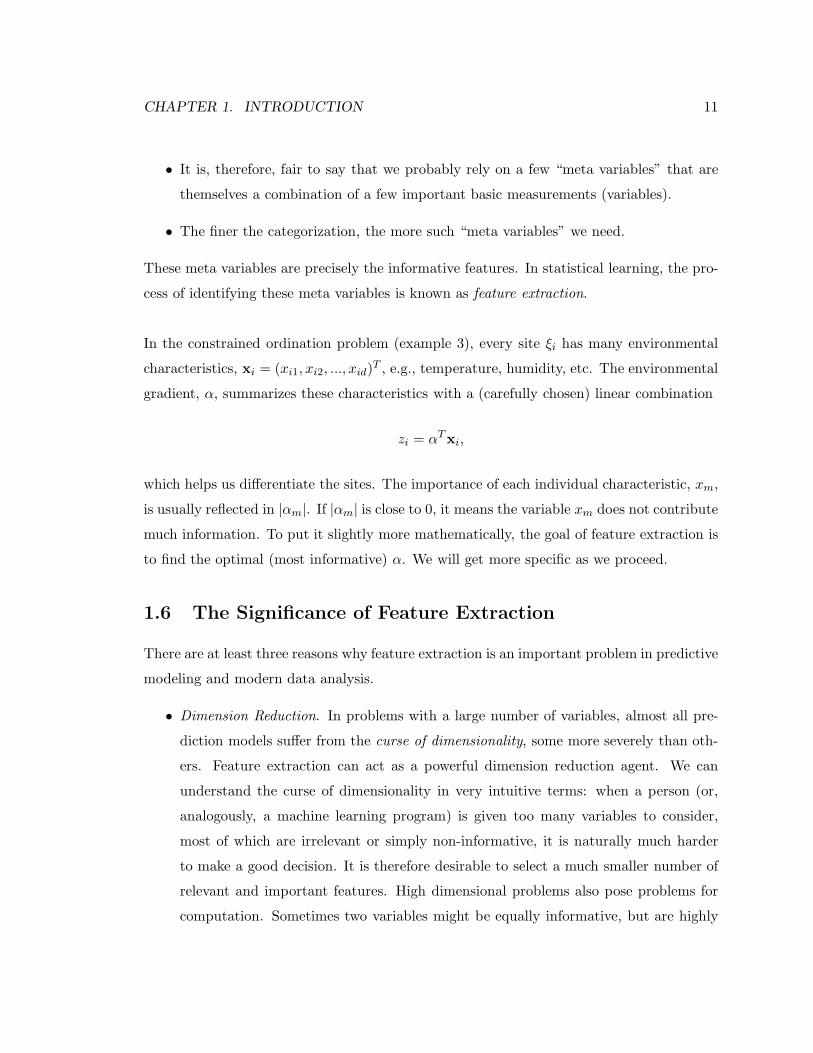
• It is, therefore, fair to say that we probably rely on a few “meta variables” that are
themselves a combination of a few important basic measurements (variables).
• The finer the categorization, the more such “meta variables” we need.
These meta variables are precisely the informative features. In statistical learning, the pro-
cess of identifying these meta variables is known as feature extraction.
In the constrained ordination problem (example 3), every site ξi has many environmental
characteristics, xi = (xi1, xi2, ..., xid)T , e.g., temperature, humidity, etc. The environmental
gradient, α, summarizes these characteristics with a (carefully chosen) linear combination
zi = αTxi,
which helps us differentiate the sites. The importance of each individual characteristic, xm,
is usually reflected in |αm|. If |αm| is close to 0, it means the variable xm does not contribute
much information. To put it slightly more mathematically, the goal of feature extraction is
to find the optimal (most informative) α. We will get more specific as we proceed.
1.6 The Significance of Feature Extraction
There are at least three reasons why feature extraction is an important problem in predictive
modeling and modern data analysis.
• Dimension Reduction. In problems with a large number of variables, almost all pre-
diction models suffer from the curse of dimensionality, some more severely than oth-
ers. Feature extraction can act as a powerful dimension reduction agent. We can
understand the curse of dimensionality in very intuitive terms: when a person (or,
analogously, a machine learning program) is given too many variables to consider,
most of which are irrelevant or simply non-informative, it is naturally much harder
to make a good decision. It is therefore desirable to select a much smaller number of
relevant and important features. High dimensional problems also pose problems for
computation. Sometimes two variables might be equally informative, but are highly
CHAPTER 1. INTRODUCTION 12
correlated with each other; this often causes ill behavior in numerical computation,
e.g., the problem of multicollinearity in ordinary least squares. Feature extraction is,
therefore, also an important computational technique.
• Automatic Exploratory Data Analysis. In many classical applications, informative
features are often selected a priori by field experts, i.e., investigators pick out what
they believe are the important variables to build a model. More and more often
in modern data-mining applications, however, there is a growing demand for fully
automated “black-box” type of prediction models that are capable of identifying the
important features on their own. The need for such automated systems arises for two
reasons. On the one hand, there are the economic needs to process large amounts of
data in a short amount of time with little manual supervision. On the other hand, it is
often the case that the problem and the data are so novel that there are simply no field
experts who understand the data well enough to be able to pick out the important
variables prior to the analysis. Under such circumstances, automatic exploratory data
analysis becomes the key. Instead of relying on pre-conceived ideas, there is a need
(as well as interest) to let the data speak for itself.
• Data Visualization. Another application of feature extraction that shares the flavor
of exploratory data analysis is data visualization. The human eye has an amazing
ability in recognizing systematic patterns in the data. At the same time, we are
usually unable to make good sense of data if it is more than three dimensional. To
maximize the use of the highly developed human faculty in visual identification, we
often wish to identify two or three of the most informative features in the data so that
we can plot the data in a reduced space. To produce such plots, feature extraction is
the crucial analytic step.
In dimension reduction, automatic exploratory data analysis and data visualization, feature
extraction is usually not the final goal of the analysis. It is an exercise to facilitate com-
putation and model building. But feature extraction can also be an important scientific
problem on its own.
Example 5 (Human Brain Mapping Project) Different parts of the human brain are

CHAPTER 1. INTRODUCTION 13
responsible for performing different tasks. In the human brain mapping project, scientists
try to understand different regions in the brain and associate each region with the primary
task it is responsible for. They do so by comparing images of the brain — obtained through
positron emission tomography (PET) or functional magnetic resonance imaging (fMRI) —
scanned while the subject performs a certain task (active state) with those scanned while
the subject rests (control state). The digitalized images consist of thousands of pixels.
Each pixel corresponds to a spot in the brain and can be treated as a variable. Rather than
building a predictive model using these variables to tell the images apart (active vs. control
state), a much more important scientific question is to identify specific regions of the brain
that are activated while the subject performs the task. In other words, the interest lies in
identifying the most important variables (pixels) that differentiate the active state from the
control state.
1.7 Organization
In this thesis, we study the feature extraction problem in its generality, with particular
focus on its applications to classification and the analysis of co-occurrence data (especially
with co-variates).
In chapter 2, we review a popular method for constrained ordination called canonical cor-
respondence analysis (CCA), originally developed by ecologists in the context of example
3. We then establish a formal equivalence between CCA and a well-known classification
technique called linear discriminant analysis (LDA). This connection provides us with some
crucial insights and makes various techniques for discriminant analysis readily applicable to
the analysis of co-occurrence data. However, there are some apparent limitations to CCA.
We show how we can understand these limitations in terms of the restrictive assumption of
LDA, and how one can overcome the limitations of CCA by generalizing LDA to quadratic
and, ultimately, non-parametric discriminant analysis. The restrictive assumption in LDA
is that the density function in each class is modeled as a Gaussian with a common covari-
ance matrix across all classes. By non-parametric discriminant analysis, we mean that the
density function in each class is modeled non-parametrically.
CHAPTER 1. INTRODUCTION 14
Before we proceed, we first provide an overview of various techniques for classification in
chapter 3. This material is relevant because in our development, we make various connec-
tions and references to other classification methods. An overview of this kind also makes it
clear where our work should fit in the vast amount of literature in classification and pattern
recognition.
The problem of non-parametric discriminant analysis is then studied in some detail in
chapters 4, 5 and 6, which constitute the main segments of the thesis.
In chapter 7, we revisit a related approach in discriminant analysis: namely, mixture dis-
criminant analysis (MDA), developed by Hastie and Tibshirani in [20]. We focus on an
extension to MDA, previously outlined in [22] but not fully studied. It turns out that this
extension actually corresponds to a natural generalization of Hofmann’s aspect model when
we have covariates on each ξi ∈ X .

Chapter 2
Co-occurrence Data and
Discriminant Analysis
In section 1.4, we came across the problem of analyzing co-occurrence data with covariates.
Example 3 depicts the canonical case (an application in the field of environmental ecology)
where an extension to correspondence analysis, known as canonical correspondence analysis
(CCA), was first developed. In this chapter, we give a detailed review of CCA and show
that it is equivalent to linear discriminant analysis (LDA), a classification technique with a
feature extraction component. Although in the ecological literature, people have made vague
connections between CCA and other multivariate methods such as LDA, the equivalence
has never been explicitly worked out and is not widely known. In the context of this thesis,
the equivalence between CCA and LDA serves as vivid testimony that the feature extraction
problem (the main topic of this thesis) is a fundamental one in statistics and is of interest
to a very broad audience in the scientific and engineering community.
2.1 Correspondence Analysis with Covariates
Suppose that associated with each category ξi ∈ X , there is a vector of covariates, xi =
(xi1, xi2, ..., xid)T ; one can then constrain the score zi to be a function of xi, the simplest
15

CHAPTER 2. CO-OCCURRENCE DATA AND DISCRIMINANT ANALYSIS 16
one being a linear function of the form
zi =
d∑
m=1
αmxim,
or in matrix form
z = Xα.
This is known as canonical correspondence analysis (CCA) and was first developed by Ter
Braak in [38]. The vector α defines (concretely) an ordination axis in the space spanned by
the covariates and is a direction in which the ηk’s and ξi’s can be easily differentiated. An
immediate advantage of this approach is that the ordination axis, instead of being a latent
scale, is now expressed in terms of the covariates; this allows easy interpretation.
The standard implementation is to insert a regression step into the reciprocal averaging
algorithm for correspondence analysis (algorithm 1.1). Note step (4) in algorithm 2.1 is
Algorithm 2.1 Iterative CCA
1. Start with an arbitrary initial vector z = z0 6= 1, properly standardized.
2. Let u = B−1Y T z.
3. Let z∗ = A−1Y u.
4. Let α = (XT AX)−1XT Az∗.
5. Let z = Xα and standardize z.
6. Alternate between steps (2) and (5) until convergence.
merely the weighted least-squares equation to solve for α. For more details, see [38]. It is
easy to see that the iteration algorithm solves for α and u that simultaneously satisfy
Xα ∝ A−1Y u

CHAPTER 2. CO-OCCURRENCE DATA AND DISCRIMINANT ANALYSIS 17
and
u ∝ B−1Y T Xα.
These are the same equations as the ones for correspondence analysis, except that z is
now expressed in the form of z = Xα. We now show that CCA is in fact equivalent to a
well-known classification technique called linear discriminant analysis (LDA).
2.2 Linear Discriminant Analysis (LDA)
2.2.1 Gaussian Discrimination
Given data yi, xini=1, where yi ∈ 1, 2, ...,K is the class label, and xi ∈ Rd is a vector
of predictors, the classification problem is to learn from the data a prediction rule which
assigns each new observation x ∈ Rd to one of the K classes. Linear discriminant analysis
assumes that x follows distribution pk(x) if it is in class k, and that
pk(x) ∼ N(µk,Σ)
Notice the covariance matrix is restricted to being the same for all K classes, which makes
the decision boundary linear between any two classes and, hence, the name linear discrim-
inant analysis. In particular, the decision boundary between any two classes j and k is
(assuming equal prior probabilities)
logp(y = j|x)
p(y = k|x)= 0 ⇐⇒ log
pj(x)
pk(x)= 0
or
(x− µj)T Σ−1(x− µj)− (x− µk)
T Σ−1(x− µk) = 0, (2.2.1)
a linear function in x because the quadratic terms xT Σ−1x cancel out. The distance
dM (x, µk)= (x− µk)
T Σ−1(x− µk) (2.2.2)

CHAPTER 2. CO-OCCURRENCE DATA AND DISCRIMINANT ANALYSIS 18
is known as the Mahalanobis distance from a point x to class k.
2.2.2 Linear Discriminant Directions
There is another way to formulate the LDA problem, first introduced by Fisher in [8].
Given data yi, xini=1, where yi ∈ 1, 2, ...,K is the class label and xi ∈ Rd is a vector of
predictors, we look for a direction α ∈ Rd in the predictor space in which the classes are
separated as much as possible. The key question here is: what is an appropriate measure
for class separation? Later we shall come back to address this question in more detail in
section 4.3. For now, it suffices to say that when Fisher first introduced this problem, he
used the following criterion:
maxα
αT Bα
αT Wα, (2.2.3)
where B is the between-class covariance matrix and W , the within-class covariance matrix.
Given any direction α ∈ Rd, if we project the data onto α, then the numerator of (2.2.3) is
the marginal between-class variance and the denominator, the marginal within-class vari-
ance. Hence large between-class variability (relative to the within-class variability) is used
as an indicator for class separation. This criterion has a great intuitive appeal, and the
solution to this optimization problem can be obtained very easily. From Appendix A, we
know that the optimal solution is simply the first eigenvector of W−1B. The solution to
this problem is usually called the linear discriminant direction or canonical variate.
In general, the matrix W−1B has min(K−1, d) non-zero eigenvalues. Hence we can identify
up to this number of discriminant directions (with decreasing importance). In fact, given
the first (m− 1) discriminant directions, the m-th direction is simply
argmaxα
αT Bα
αT Wαsubject to αT Wαj = 0 ∀ j < m.
This is the feature extraction aspect of LDA. The optimal discriminant directions are the
extracted features; they are the most important features for classification.

CHAPTER 2. CO-OCCURRENCE DATA AND DISCRIMINANT ANALYSIS 19
2.2.3 Connections
The two seemingly unrelated formulations of LDA are, in fact, intimately connected. From
equation (2.2.1) we can see that a new observation x is classified to the class whose centroid
is the closest to x in Mahalanobis distance. For a K-class problem, the K class centroids
lie on a (K − 1)-dimensional subspace, S. Therefore, one can decompose dM (x, µk) into
two orthogonal components, one lying within S and one orthogonal to S. The orthogonal
components are the same for all x and are therefore useless for classification. It is usually
the case that d≫ K. It can be shown (see [20]) that the K− 1 discriminant directions also
span the subspace S. What’s more, let A be the (K − 1)-by-d matrix stacking α1, ..., αK−1
as row vectors, and define
x∗ = Ax,
µ∗k = Aµk,
and it can be shown (see [20]) that classification based on Mahalanobis distances is the
same as classification based on Euclidean distances in the new x∗-space:
class(x) = argmink
‖x∗ − µ∗k‖.
What is more, if we use only the first M < K − 1 discriminant directions for classification,
it can be shown (see [20]) that this is the same as doing LDA using the usual Mahalanobis
distance but constraining the K class centroids to lie in an M -dimensional subspace. This
is called reduced-rank LDA. It is often the case that reduced-rank LDA has a lower misclas-
sification rate than full-rank LDA on test data. The reason for the improved performance
is, of course, well-known: by using only the leading discriminant directions, we have thrown
away the noisy directions and avoided over-fitting. Therefore, reduced-rank LDA is a vivid
example of the practical significance of feature extraction.

CHAPTER 2. CO-OCCURRENCE DATA AND DISCRIMINANT ANALYSIS 20
2.3 Equivalence Between CCA and LDA
It is known that correspondence analysis, canonical correlations, optimal scoring and linear
discriminant analysis are equivalent (e.g., [17] and [18]). Since canonical correspondence
analysis is simply an extension of correspondence analysis, its equivalence to canonical cor-
relations and discriminant analysis should follow directly. This equivalence, however, is not
widely known. In this section, we shall formally derive the equivalence.
Heuristically, an easy way to understand the equivalence is through the optimal scoring
problem:
minθ,β;‖Y θ‖=1
‖Y θ −Xβ‖2.
If we expand the co-occurrence matrix into two indicator matrices, one by row (X), and
another by column (Y ), as illustrated in table 2.1; and if we do optimal scoring on Y and
X, then it is well-known (e.g., [17] and [30]) that the optimal scores, θ and β, are the same
as the row and column scores, u and z, from correspondence analysis. Moreover, if we treat
YN×K XN×I
Obs η1 ... ηK ξ1 ... ξI
1 1 ... 0 1 ... 02 1 ... 0 1 ... 0...
.... . .
......
. . ....
N 0 ... 1 0 ... 1
Table 2.1: Co-occurrence data represented by two indicator matrices, Y and X. For exam-ple, for every count of (η3, ξ2) co-occurrence, a row (0, 0, 1, 0, ..., 0) is added to Y and a row(0, 1, 0, ..., 0) is added to X.
the ηk’s as K classes and the ξi’s as I (categorical) predictors (each represented by a binary
indicator as in matrix X), then the optimal score β is also the same as the best linear
discriminant direction, aside from a scaling factor.
If each ξi is associated with a set of covariates, xi = (xi1, xi2, ..., xid)T , then we can expand
the co-occurrence matrix into indicator matrices as before, one by row (X) and another
CHAPTER 2. CO-OCCURRENCE DATA AND DISCRIMINANT ANALYSIS 21
YN×K XN×d
Obs η1 ... ηK x1 ... xd
1 1 ... 0 x11 ... x1d
2 1 ... 0 x21 ... x2d...
.... . .
......
. . ....
N 0 ... 1 xN1 ... xNd
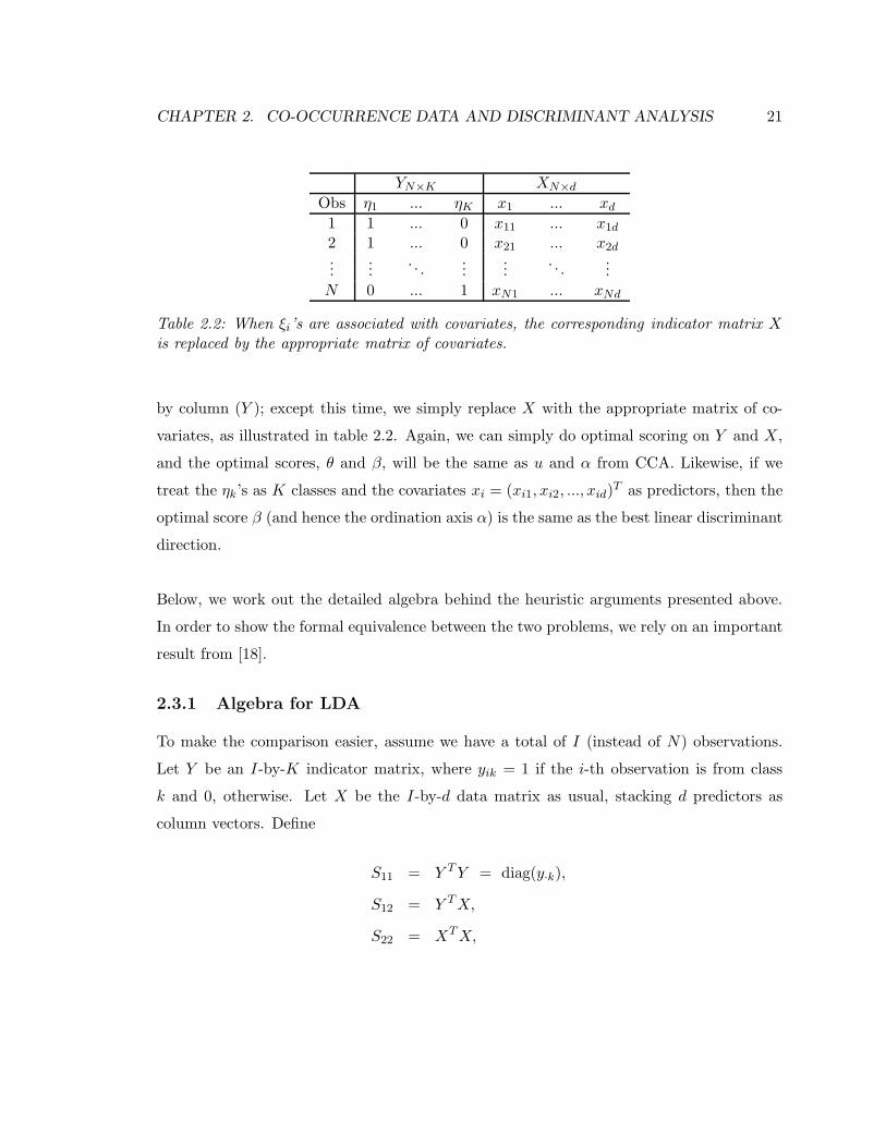
Table 2.2: When ξi’s are associated with covariates, the corresponding indicator matrix Xis replaced by the appropriate matrix of covariates.
by column (Y ); except this time, we simply replace X with the appropriate matrix of co-
variates, as illustrated in table 2.2. Again, we can simply do optimal scoring on Y and X,
and the optimal scores, θ and β, will be the same as u and α from CCA. Likewise, if we
treat the ηk’s as K classes and the covariates xi = (xi1, xi2, ..., xid)T as predictors, then the
optimal score β (and hence the ordination axis α) is the same as the best linear discriminant
direction.
Below, we work out the detailed algebra behind the heuristic arguments presented above.
In order to show the formal equivalence between the two problems, we rely on an important
result from [18].
2.3.1 Algebra for LDA
To make the comparison easier, assume we have a total of I (instead of N) observations.
Let Y be an I-by-K indicator matrix, where yik = 1 if the i-th observation is from class
k and 0, otherwise. Let X be the I-by-d data matrix as usual, stacking d predictors as
column vectors. Define
S11 = Y T Y = diag(y·k),
S12 = Y T X,
S22 = XT X,

CHAPTER 2. CO-OCCURRENCE DATA AND DISCRIMINANT ANALYSIS 22
with S21 = ST12 = XT Y . It is shown in [18] that the discriminant direction, α, can also be
obtained by solving the following canonical correlations problem (up to a scale factor):
maxα, u
uT S12α
s.t.
αT S22α = 1 and uT S11u = 1.
The solution to this problem is, of course, standard (e.g., Appendix A of [17]). We simply
apply the singular value decomposition (SVD) to the matrix
M = S−1/211 S12S
−1/222 .
Suppose the first right singular vector is α∗; then the best α is simply given by
α = S−1/222 α∗.
By the well-known connection between SVD and spectral decomposition of symmetric ma-
trices, α∗ is also the first eigenvector of
MT M = S−1/222 S21S
−111 S12S
−1/222 .
It is also easy to see that if x is an eigenvector of P−1/2QP−1/2, then P−1/2x is an eigenvector
of P−1Q, e.g., Theorem A.9.2. of [30]. Therefore, this implies the discriminant direction,
α = S−1/222 α∗, is simply an eigenvector of
Γα = S−122 S21S
−111 S12.
Similarly, from the left singular vectors of M , or eigenvectors of MMT , we can see that u
is an eigenvector of
Γu = S−111 S12S
−122 S21.

CHAPTER 2. CO-OCCURRENCE DATA AND DISCRIMINANT ANALYSIS 23
2.3.2 Algebra for CCA
In CCA, Y is an I-by-K co-occurrence matrix and X an I-by-d matrix of covariates. We’ve
shown in section 2.1 that the essence of CCA is to solve simultaneously for α and u from
Xα ∝ A−1Y u and u ∝ B−1Y T Xα,
where, again, A = diag(yi·) and B = diag(y·k) (see section 1.2). Noting that X is not a
square matrix and, hence, not invertible, whereas XT AX is, we get
α ∝(
(
XT AX)−1
XT Y)
u,
u ∝(
B−1Y T X)
α,
which leads us to a set of eigen-equations:
α ∝(
(
XT AX)−1
XT Y)
(
B−1Y T X)
α,
u ∝(
B−1Y T X)
(
(
XT AX)−1
XT Y)
u.
To see the equivalence between CCA and LDA, simply write
S11 = B = diag(y·k),
S12 = Y T X,
S22 = XT AX,
with S21 = ST12 = XT Y , and we can see that ordination direction, α, is simply an eigenvector
of
Ψα = S−122 S21S
−111 S12
and u, an eigenvector of
Ψu = S−111 S12S
−122 S21.

CHAPTER 2. CO-OCCURRENCE DATA AND DISCRIMINANT ANALYSIS 24
2.3.3 Algebraic Equivalence
Now compare the Ψ’s with the Γ’s, and it is clear that the only “difference” between the or-
dination direction and the discriminant direction lies in the differences between S22 and S22.
This “difference,” however, can be easily removed upon noticing that data matrices, X
and Y , are organized differently for the two problems. For the discrimination problem,
each row contains information for exactly one observation (occurrence). For the CCA prob-
lem, however, each row contains information for all observations (occurrences) of ξi. Instead
of being a binary indicator, each entry of Y , yik, is the count of the total number of ob-
servations (occurrences) of ηk and ξi together. These observations, regardless of their class
membership (ηk), share the same row in the covariate matrix X. Therefore, the i-th row of
X must be weighted by the total number of ξi, which is yi· =∑K
k=1 yik. The proper weight
matrix, then, is given by
diag(yi·) = A.
Therefore, S22 = XT AX is simply the properly weighted version of S22 = XT X.
To this effect, if we rearrange the matrices Y and X to fit the standard format for dis-
criminant analysis and compute Γ, we obtain exactly the same matrix Ψ. Thus, to obtain
the ordination direction, we can form the matrix Ψ as usual from Y and X and find its
eigen-decomposition. Alternatively, we can first expand the matrices Y and X to contain
exactly one observation per row — the i-th row of Y will be expanded into a total of yi·
rows, each being a binary indicator vector; the i-th row of X will be replicated yi· times
(since all yi· observations share the same xi) to form the expanded version of X. We can
then obtain the ordination direction by doing an eigen-decomposition on Γ, constructed
from the expanded versions of Y and X.
Remark 2.1 Our argument shows that the equivalence between canonical correspondence
analysis and discriminant analysis can be derived using well-known results in multivariate
analysis and matrix algebra. But this connection is not widely understood. The disguise is

CHAPTER 2. CO-OCCURRENCE DATA AND DISCRIMINANT ANALYSIS 25
perhaps largely due to the different ways the data are organized. This is a vivid example
of how the seemingly trivial task of data organization can profoundly influence statistical
thinking.
2.3.4 Model Equivalence
We now point out a direct connection between the probabilistic models for discriminant
analysis and the Gaussian response model for co-occurrence data (see example 2, p. 4),
without referring to optimal scoring or canonical correlations as an intermediate agent.
Consider the space E spanned by the covariates, xm,m = 1, 2, ..., d. Every ξi can then
be mapped to a point xi = (xi1, xi2, ..., xid)T ∈ E , and the relative frequency of ηk can be
described by a response function pk(x) in E . Now think of this as a K-class classification
problem, where the ηk’s are the classes and pk(x) is the density function for class k (or
ηk). The quantity of interest for classification is the posterior probability of class k given
a point xi ∈ E , i.e., P (y = k|x = xi), or P (ηk|ξi), the conditional occurrence probability
of ηk given ξi. Suppose pk(x) is Gaussian with mean µk and covariance Σk. This means
µk is the optimal point for class k (or ηk) in the sense that the density for class k (or the
relative frequency for ηk) is high at µk ∈ E . In terms of co-occurrence data, this means for
any given ξi, if xi = µk, then the co-occurrence between ξi and ηk will be highly likely.
The ordination axis is a vector α ∈ E . Now let uk, zi be the projections of µk, xi onto
α, respectively, and let fk(z) be the projection of pk(x) on α. It follows that fk(z) is a
univariate Gaussian curve, with mean uk and variance t2k, where
t2k= αT Σkα.
Now let πk be the prior (occurrence) probability of class k (or ηk), then by Bayes Theorem
and using information in the direction of α alone, we get
P (ηk|ξi) = P (y = k|z = zi) ∝ πkfk(zi) ∝(
πk
tk
)
exp
−(zi − uk)2
2t2k
,

CHAPTER 2. CO-OCCURRENCE DATA AND DISCRIMINANT ANALYSIS 26
or
log P (y = k|z = zi) = bk −(zi − uk)
2
2t2k, (2.3.4)
where we have collapsed the proportionality constant, the prior probability πk and the tol-
erance parameter tk into a single constant bk.
Now recall the Gaussian response model (example 2), where yik ∼ Poisson(λik). It fol-
lows that conditional on ξi,
(
(yi1, yi2, ..., yiK)
∣
∣
∣
∣
K∑
k=1
yik = Ni
)
∼ Multinomial
(
Ni; pi1 =λi1
Ni, pi2 =
λi2
Ni, ..., piK =
λiK
Ni
)
,
where pik is the conditional probability of ηk given ξi. So directly from the Gaussian response
model, we can also derive that
log pik = log λik − log Ni = ak −(zi − uk)
2
2t2k− log Ni = bk −
(zi − uk)2
2t2k,
where bk = ak − log Ni. Note that since the probability is conditional on ξi, Ni can be
considered a constant.
Therefore, the Gaussian response model for co-occurrence data is the same as the (low-
rank) Gaussian model for discriminant analysis in the sense that they specify exactly the
same posterior probabilities, P (ηk|ξi) and P (y = k|z = zi). Recall from example 2 that
CCA further assumes that the tolerance level is the same for all ηk, which, in the discrimi-
nation context, is equivalent to assuming that all classes have the same covariance matrix,
i.e., LDA.
2.4 Flexible Response Curves and Flexible Class Densities
Let us now summarize what we learned from our discussions above and gain some important
insights:
• Algebraically, the discriminant directions in LDA are equivalent to the ordination axes
CHAPTER 2. CO-OCCURRENCE DATA AND DISCRIMINANT ANALYSIS 27
in CCA.
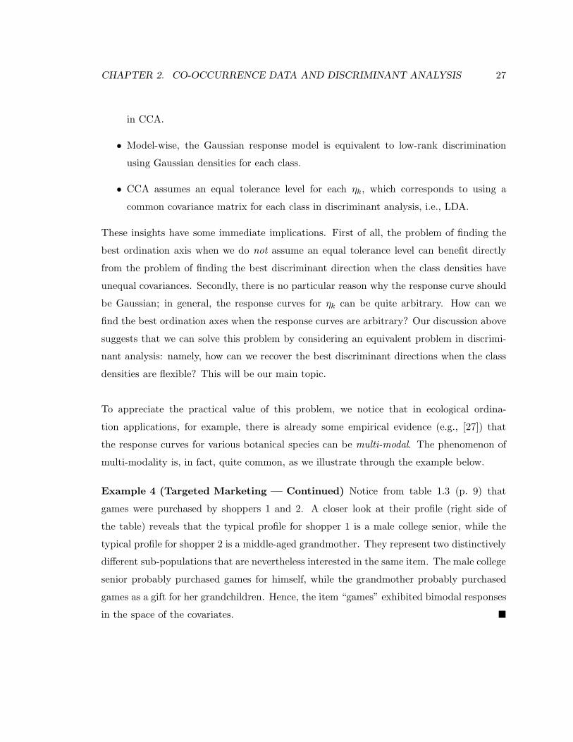
• Model-wise, the Gaussian response model is equivalent to low-rank discrimination
using Gaussian densities for each class.
• CCA assumes an equal tolerance level for each ηk, which corresponds to using a
common covariance matrix for each class in discriminant analysis, i.e., LDA.
These insights have some immediate implications. First of all, the problem of finding the
best ordination axis when we do not assume an equal tolerance level can benefit directly
from the problem of finding the best discriminant direction when the class densities have
unequal covariances. Secondly, there is no particular reason why the response curve should
be Gaussian; in general, the response curves for ηk can be quite arbitrary. How can we
find the best ordination axes when the response curves are arbitrary? Our discussion above
suggests that we can solve this problem by considering an equivalent problem in discrimi-
nant analysis: namely, how can we recover the best discriminant directions when the class
densities are flexible? This will be our main topic.
To appreciate the practical value of this problem, we notice that in ecological ordina-
tion applications, for example, there is already some empirical evidence (e.g., [27]) that
the response curves for various botanical species can be multi-modal. The phenomenon of
multi-modality is, in fact, quite common, as we illustrate through the example below.
Example 4 (Targeted Marketing — Continued) Notice from table 1.3 (p. 9) that
games were purchased by shoppers 1 and 2. A closer look at their profile (right side of
the table) reveals that the typical profile for shopper 1 is a male college senior, while the
typical profile for shopper 2 is a middle-aged grandmother. They represent two distinctively
different sub-populations that are nevertheless interested in the same item. The male college
senior probably purchased games for himself, while the grandmother probably purchased
games as a gift for her grandchildren. Hence, the item “games” exhibited bimodal responses
in the space of the covariates.

CHAPTER 2. CO-OCCURRENCE DATA AND DISCRIMINANT ANALYSIS 28
2.5 The Limitations of LDA
To further motivate our study, we now construct an example where LDA is clearly insuffi-
cient.
Example 6 (Bimodality) The left panel in figure 2.1 shows a case where x = (x1, x2)T
is uniform inside the unit square (0, 1)2 and
y =
2 if x1 ∈(
13 , 2
3
)
,
1 otherwise.
In this case it is obvious that x1 is the important discriminant direction. But LDA consis-
Data
0.0 0.2 0.4 0.6 0.8 1.0
0.0
0.2
0.4
0.6
0.8
1.0
1
1
1
1
1
1
1
1
1
1
1
11
1
2
2
2
1
1
11
1
1
2
2
1
2
1
2
1
1
2
2
1
1
1
2
1
1
1
1
2
2
1
2
2
2
1
2
1
1
2
2
1
21
1
1
1
1
1
1
2
2
1
2
1
1
1
2
2
2
1
1
1
2
2
2
2
2
1
1
1
11
1
2
2 1
2
1
1
2
1
1
1
1
22
2
1
1
2
1
2
1
2
1
1
1
1
1
1
1
2
1
2
2 1
1
2
2
1
1
1
2
211
1
21
1
1
2
1
11
1
11
1
1
1
1
2
2
2
2
2 1
1
2
1
1
1
2
2
2
2
1
1
2
1
2
1
1
22
1
2
1
2
2
2
1
1
1
2
1
2
111
1
1
1
1
2
12
1
1
1
2
1
2
2
1
1
2
2 2
11
2
2
1
2
2
1
11
1
2
1
1
2
1 2
2
1
1
1
22
2
12
1
1 1
2
1
1
1
1
2
1
1
1
21
1
1
1
1
2
1
2
1
1
1
1 2
1
1
2
1
1
1
1
1
2
2
1
1
2
1
2
1
1
1
1
1
2
1
1
2
1
2
11
1
1
1
1
12
2
1
2
2
12
11
1
1
1
12
1
1
2
1
1
1
11
2
1
1
1
2
1
12
2
2
2
1
2
1
2
1
1
2
2
2
1
1
22
1
2
2
1
1
1
1
1
12
1
1
1
2
2
1
1
1
11
2
11
2
1
1
1
1
1
21
1
1
1
1
2
2
2
2
2
1
2
2
1
2
11
21
1
2
2
1
2
2
1
2
2
1
1
1
1
1
2
2
2
1
1
2
1
2
2
1
1
2
2
22
1
1
1
2
1
2
1
1
11
1
2
2
12
12
2
1
1
2
1
1
1
2
2
2
1
1
2
2
2
1
12
21
2
2
1
1
1
2
1
2
2
2
2
1
1
1
1
2
2 1
1
1
2
2
2
1
1
1
11
2
2
1
2
1
1
1
2
1
1
1
1
2
21
2
1
2
1
2
1
1
2
0.0 0.2 0.4 0.6 0.8 1.0
05
1015
LDA
Figure 2.1: Left: The horizontal axis is clearly the best discriminant direction for this case.Right: Histogram (100 simulations) of cos(θ), where θ is the acute angle formed betweenthe horizontal axis and the discriminant direction resulting from LDA. LDA clearly fails torecover the best discriminant direction.
tently fails to find this direction as the discriminant direction. We simulated this situation
100 times. Each time, we computed the cosine of the acute angle formed between the
horizontal axis and the discriminant direction obtained from LDA. If LDA were to work
correctly, we’d expect most of these values to be close to 1. The right panel of figure 2.1
shows that this is not the case at all.
The reason why LDA fails in example 6 is that the class centroids coincide, i.e., there is no
discriminatory information in the class means — all such information is contained in the
variances of the two classes. This points out a fundamental limitation of LDA. As we shall

CHAPTER 2. CO-OCCURRENCE DATA AND DISCRIMINANT ANALYSIS 29
show in chapter 4, LDA is guaranteed to find the optimal discriminant directions when the
class densities are Gaussian with the same covariance matrix for all the classes. But when
the class densities become more flexible, LDA can fail, such as in example 6.
Remark 2.2 Later we found a specific proposal elsewhere (section 9.8 of [6]) which ad-
dresses the problems illustrated in example 6. Their specific method, however, can only
extract one type of discriminatory information, i.e., when all such information is contained
in the variances but not in the centroids. Consequently, the method is not of much practical
value. It is interesting to note that the authors did express regret in their writing that a
direct feature extraction method “capable of extracting as much discriminatory informa-
tion as possible regardless of its type” would require a “complex criterion” which would be
“difficult to define” (p. 339). By the end of this thesis, all such difficulties will have been
resolved and we shall see that the “complex criterion” is not so complex after all.
2.6 Summary
By now, it should be clear that the ordination axis in the analysis of co-occurrence data
is the same mathematical concept as the discriminant direction in classification problems.
There is also an intuitive reason behind this mathematical equivalence: Both the ordina-
tion axis and the discriminant direction are projections in which items, or classes, are easily
differentiable — it is a direction in which similar items come together and different items
come apart. In chapter 1, we referred to such projections as informative features.
We are now ready to move on to the main part of this thesis, where we shall focus on
the generalization of LDA, which will ultimately allow us to find the most informative fea-
tures when the class densities are quite arbitrary. The underlying equivalence between CCA
and LDA implies that our generalization will allow ecologists to solve the constrained ordi-
nation problem without restricting the response curves to lie in any particular parametric
family.

Chapter 3
Classification
Linear discriminant analysis (LDA) is a basic classification procedure. In this chapter, we
offer a systematic review of various techniques for classification. This material will allow us
to make various connections between our work and the existing literature.
From a statistical point of view, the key quantity of interest for classification is the posterior
class probability: P (y = k|x). Once this is known or estimated, the best decision rule is
simply
y = argmaxk=1,2,...,K
P (y = k|x),
provided that the costs of misclassification are equal. The statistical problem of classi-
fication, therefore, can usually be formulated in terms of a model for the posterior class
probabilities, i.e.,
P (y = k|x) = gk(x).
By selecting gk from different functional classes, one can come up with a great variety of
classification models. We shall review a few of the most widely used models for gk in section
3.1. This formulation puts the classification problem in parallel with the other statistical
learning problem where the response is continuous, namely, regression. Recall the regression
30

CHAPTER 3. CLASSIFICATION 31
function is simply
E(y|x) = g(x)
for y ∈ R. Thus in the regression problem, we try to estimate the conditional expectation;
in the classification problem, we try to estimate the conditional probability. The key point
here is that the model is always regarded as being conditional on x, so the marginal infor-
mation in x is not used.
A slightly different formulation that uses the marginal information in x is possible. By
Bayes Theorem,
P (y = k|x) ∝ πkpk(x),
where πk is the prior probability of class k and pk(x), the density function of x conditional
on the class label k. Here the methods will differ by choosing the pk’s differently. We shall
review some of the most widely used models for pk(x) in section 3.2.
These two approaches are apparently not completely independent of one another. A certain
model for pk, for example, will correspond to a certain model for gk. We briefly discuss this
correspondence in section 3.3.
3.1 Modeling Posterior Probabilities
3.1.1 Logistic Regression
To start our discussion, recall the basic binary-response logistic regression model:
logP (y = 1|x)
P (y = 0|x)= β0 +
d∑
m=1
βmxm. (3.1.1)
The left-hand side is usually called the log-odds. One reason why we model the log-odds
rather than the posterior probability itself is because a probability must lie between 0 and 1,

CHAPTER 3. CLASSIFICATION 32
whereas the log-odds can take values on (−∞,∞), making it easier to model. A deeper rea-
son is because the binomial distribution belongs to an exponential family and the log-odds
is actually its natural parameterization. The coefficients in this model can be estimated by
maximum likelihood via iterative re-weighted least-squares (IRLS). For more details, see
[31].
The basic logistic regression model is a very common tool for a two-class classification
problem. When there are K > 2 classes, this model generalizes to
logP (y = k|x)
P (y = K|x)= βk0 +
d∑
m=1
βkmxm (3.1.2)
for k = 1, 2, ...,K − 1.
3.1.2 Generalized Additive Models (GAM)
We can further generalize the logistic regression model to allow a transformation on each
predictor before it enters the model:
logP (y = k|x)
P (y = K|x)= βk0 +
d∑
m=1
βkmfkm(xm). (3.1.3)
These models are called Generalized Additive Models. Of course, we have to put some
restrictions on fkm. Usually a smoothness constraint is imposed by adding a penalty term
to the log-likelihood such as
d∑
m=1
λkm
∫ ∞
−∞
(
f′′
km(xm))2
dxm.
Typically, additive models are fitted iteratively by back-fitting. For generalized additive
models, it is necessary to combine the IRLS algorithm with back-fitting. For more details,
see [19].

CHAPTER 3. CLASSIFICATION 33
3.1.3 Projection Pursuit Logistic Regression
Yet another level of generalization can be achieved, for example, by considering
logP (y = k|x)
P (y = K|x)= βk0 +
M∑
m=1
βkmfkm(αTkmx). (3.1.4)
Besides fitting the smooth functions fkm, we must fit the αkm’s as well. Again, the model
is fitted iteratively. For fixed αkm’s, the model is the same as (3.1.3). For fixed fkm’s, the
αkm’s can be estimated by the Gauss-Newton algorithm, where, of course, we will need to
estimate f′
km as well. Therefore this model is fitted by embedding a Gauss-Newton loop
into a back-fitting loop, which is then embedded into the standard IRLS loop for logistic
regression. See [34] for more details.
Theoretically, this model is important because it has been shown in [7] that the right-
hand side is flexible enough to approximate any smooth function provided that M is large
enough. The work which we shall present in Chapter 6 is closely related to a special case
of this model. We shall then come back to this point.
3.2 Modeling Class Densities
There is a connection between classification, hypothesis testing and density estimation. For
any two classes i, j, the posterior odds is simply the prior odds times the likelihood ratio:
P (y = i|x)
P (y = j|x)=
(
πi
πj
)(
pi(x)
pj(x)
)
.
Therefore, instead of specifying a model for the posterior class probabilities, a classification
problem can also be approached by specifying a model for the class-densities, pk(x). For
simplicity, we will assume πk = 1/K ∀ k for the rest of our discussion.

CHAPTER 3. CLASSIFICATION 34
3.2.1 Gaussian Discrimination
We start with pk(x) ∼ N(µk,Σk). In this case, an observation will be classified to
argmaxk=1,2,...,K
P (y = k|x) = argmaxk
log P (y = k|x)
= argmaxk
log pk(x)
= argmink
(
(x− µk)T Σ−1
k (x− µk)
2+
log 2π|Σk|2
)
= argmink
(dM (x;µk,Σk) + constk) ,
where dM (x;µk,Σk) is the well-known (and familiar) Mahalanobis distance (see section 2.2).
In this setting, the decision boundary between classes i and j is
bi,j = x : dM (x;µi,Σi) + log |Σi| = dM (x;µj ,Σj) + log |Σj |.
The simplest case here is to assume the classes share the same covariance structure, namely
Σ1 = Σ2 = ... = ΣK . In this case, the quadratic term, xT (Σi − Σj)x, drops out and the
decision boundary becomes linear (LDA). We already reviewed this important material in
section 2.2.
The equal-covariance assumption is a strong one and it creates a big bias. Quadratic
discriminant analysis, or QDA, allows Σk’s to vary; this produces a quadratic decision
boundary; and, hence, the name. Although QDA reduces the bias of LDA, it does so by
making a sacrifice in the variance. In particular, the number of parameters to be estimated
is
Kd + Kd(d + 1)
2.
For high-dimensional problems when d is large, the problem can become ill-posed. For this
reason, LDA is still a popular method despite its bias. Due to its low variance and stability,
it sometimes outperforms the less restrictive methods even when the assumptions are clearly
violated.

CHAPTER 3. CLASSIFICATION 35
3.2.2 Regularization
Regularization can improve the performance of QDA. In [12], the covariance matrices are
shrunk twice: once toward a pooled estimate, and once toward the identity matrix. In
particular, let S be the pooled sample covariance. It is suggested that we take
Sk(λ) = λSk + (1− λ)S,
and
Sk(λ, γ) = γSk(λ) + (1− γ)tr
(
Sk(λ)
p
)
I,
and use Sk(λ, γ) as the proper estimate of Σk. The λ = 0 case corresponds to LDA, and
the λ = 1 case corresponds to QDA. Thus, Sk(λ) shrinks Sk toward a pooled estimate
and becomes more stable than Sk. The motivation behind shrinking Sk(λ) further toward
the identity matrix is slightly deeper. Recall that for Gaussian discrimination, the decision
boundary depends on dM (x;µk,Σk), the Mahalanobis distance. The spectral decomposition
of Σk gives
Σk = VkDkVTk =
d∑
i=1
dikvikvTik.
Therefore,
Σ−1k =
d∑
i=1
(
vikvTik
dik
)
,
and
dM (x;µk,Σk) =
d∑
i=1
(
(
vTik(x− µk)
)2
dik
)
.
Hence directions associated with the small eigenvalues are weighted more heavily for clas-
sification. But at the same time, it is a well-known fact that the sample covariance matrix
S tends to overestimate the large eigenvalues and underestimate the small eigenvalues of
Σ. Shrinking the covariance matrices toward the identity is aimed at correcting this problem.
CHAPTER 3. CLASSIFICATION 36
Another (more classical) approach for regularization is to impose some structure on the
covariance matrices. A systematic treatment is given in [1], where structures of various lev-
els of flexibility are imposed on the covariance matrices based on their eigen-decompositions:
Σk = λkBkDkBTk .
Here λk normalizes Dk so that det(Dk) = 1. This scheme also gives us a nice way to
interpret the basic elements of the covariance matrices:
• λk controls the volume,
• Bk controls the orientation of the principal axes, and
• Dk controls the shape or stretch
of the ellipsoids. Different levels of regularization can then be achieved by forcing some (but
not all) of these elements to be identical across classes. This work is based on an earlier
predecessor called the common principle component (CPC) model (see [9]). For K groups,
the CPC models them as N(µk,Σk), where
Σk = BDkBT
and Dk is a diagonal matrix, so that the column vectors of B define the set of common
principal components. A detailed description of how to fit the CPC model by maximum-
likelihood via the FG-algorithm is given in [9].
3.2.3 Flexible Decision Boundaries
For Gaussian discrimination, the decision boundaries are at most quadratic. In this regard,
flexible discriminant analysis (FDA) is proposed in [21] to accommodate even more flexible
decision boundaries. Let Y be an n × K indicator matrix and X be an n × p matrix of
predictors. Consider the optimal scoring problem, which is equivalent to LDA (see section
2.3 and [18]):
minθ,β;‖Y θ‖=1
‖Y θ −Xβ‖2.

CHAPTER 3. CLASSIFICATION 37
Here θ(Y ) = Y θ : 1, 2, ...,K 7→ R assigns each class a score, so that a classification
problem where the responses are unordered is turned into a regression problem where the
responses are ordered. For fixed θ, β = (XT X)−1XT Y θ is simply the ordinary least-squares
solution, so
θ = argmin‖Y θ‖=1
‖Y θ −X(XT X)−1XT Y θ‖2
= argmin‖Y θ‖=1
θTY T (I −H)T (I −H)Y θ where H= X(XT X)−1XT
= argmin‖Y θ‖=1
θTY T (I −H)Y θ since (I −H)T (I −H) = I −H
= argmax‖Y θ‖=1
θT Y T Y θ where Y = HY.
This gives a simple algorithm for solving the optimal scoring problem (algorithm 3.1). The
Algorithm 3.1 Optimal Scoring Algorithm
1. Let B = (XT X)−1XT Y and Y = XB.
2. Obtain θ as eigenvectors of Y T Y , subject to θT (Y T Y )θ = 1.
3. Obtain β = Bθ.
resulting β’s are equivalent to the linear discriminant directions from LDA. FDA generalizes
LDA by generalizing the regression step to allow non-parametric and adaptive regression,
e.g., smoothing-splines, MARS. Incorporating these non-parametric regression methods es-
sentially means a basis expansion on the original predictors and LDA in the expanded space.
A linear decision boundary in the expanded space becomes non-linear in the original space.
In the new (enlarged) space, LDA often becomes ill posed. A solution is provided in [18].
Simply consider a penalized optimal scoring problem of the following form:
minθ,β;‖Y θ‖=1
‖Y θ −Xβ‖2 + λβT Ωβ,
where Ω is a penalty matrix. This is called penalized discriminant analysis (PDA).
Remark 3.1 Lately, Support Vector Machine (SVM) has become a popular classifier. The

CHAPTER 3. CLASSIFICATION 38
mathematical problem for SVM is formulated as one of finding the best separating hyper-
plane. A separating hyperplane, of course, produces a linear decision boundary. There an
idea similar to that of basis expansion is used to produce non-linear decision boundaries.
Though popular and fascinating on its own, SVM is not as relevant to this thesis. More
details can be found, for example, in [14].
3.2.4 Non-Parametric Discrimination
More generally, one does not have to assume that the class densities are Gaussian. With
more flexible density functions, the decision boundaries also become more flexible. Esti-
mating a multivariate density function, however, is an extremely difficult problem due to
the curse of dimensionality. For this reason, one rarely works with non-parametric density
functions directly. Instead, various approximations have been studied. Here we review the
two most popular ones.
Example 7 (Gaussian Mixtures) Modeling each class as a mixture of Gaussians, e.g.,
pk(x) =
Rk∑
r=1
πkrφ(x;µkr,Σ),
one can approximate a more flexible non-parametric density function. Maximum likelihood
estimates for the parameters — µkr,Σ as well as the mixing proportions πkr — can be
obtained quite readily using the EM algorithm. We will come back to mixture models in
chapter 7.
Example 8 (Naive Bayes) Naive Bayes avoids multivariate densities by introducing a
strong independence assumption. For x = (x1, x2, ..., xd)T ∈ R
d, it is assumed that
pk(x) =
d∏
m=1
pkm(xm). (3.2.5)
That is, we assume the joint density for each class is simply the product of the marginal
densities. Such a strong assumption may seem unreasonable, but Naive Bayes performs
remarkably well in many classification problems and is a very popular classifier. Due to

CHAPTER 3. CLASSIFICATION 39
the independence assumption, the density function is highly biased. But this allows us to
by-pass the dimensionality problem and reduce the variance of the problem. A heuristic
but convincing argument for its good performance is that classification results depend on
the density function only through the posterior odds; therefore, it is often not necessary to
model the underlying densities perfectly. Another advantage of Naive Bayes is that it is
easy to deal with both real-valued and categorical predictors, because different models can
be used for each individual predictor.
3.2.5 Theoretical Motivation of the Thesis
Non-parametric discriminant analysis provides another motivation for the general feature
extraction problem. First of all, we notice that non-parametric discriminant analysis has
rarely been treated in the literature, and feel that some work is needed in this area. Secondly,
due to the curse of dimensionality, it is quite natural that our focus should first rest upon
the dimension reduction problem. Therefore our problem — that of extracting informative
features to separate the classes when the class densities are flexible — arises very naturally
from these considerations.
3.3 Connections
The materials in sections 3.1 and 3.2 are closely related. Different models of pk will lead to
different models of gk. A detailed study of these connections can be found in [35].
Example 9 (LDA and Logit) In LDA, pk ∼ N(µk,Σ). One can easily work out the
implied posterior odds:
logP (y = k|x)
P (y = K|x)= log
πk
πK+ log
pk(x)
pK(x)
= logπk
πK+ (µk − µK)T Σ−1x− (µk − µK)T Σ−1(µk − µK)/2
= βk0 + βT x
with βT = (µk − µK)T Σ−1, and βk0 collects all the other constant terms. So for LDA, the
posterior log odds is a linear function in x, the same as logistic regression.
CHAPTER 3. CLASSIFICATION 40
Example 10 (Naive Bayes and GAM) The posterior odds for the Naive Bayes model
is
logP (y = k|x)
P (y = K|x)= log
πk
πK+ log
pk(x)
pK(x)
= logπk
πK+
d∑
m=1
logpkm(x)
pKm(x)
= βk0 +
d∑
m=1
fkm(xm)
with fkm = log(pkm/pKm). In other words, the posterior log odds for the Naive Bayes
method is an additive model in x.
So what’s the difference? The main difference is that the models are estimated differently.
In logistic regression and GAM, the parameters are estimated by maximizing the conditional
likelihood. In LDA and Naive Bayes, the parameters are estimated by maximizing the full
likelihood. There are different advantages to both approaches. We will not go into details
here, but refer interested readers to [35].
3.4 Other Popular Classifiers
There are, of course, many other classifiers: e.g., neural networks, CART (Classification
and Regression Trees), SVM (Support Vector Machines) and K-nearest neighbor. A very
good review can be found in [14]. Both neural networks and CART can be thought of as
using even more complicated functions gk to model the posterior probability P (y = k|x).
K-nearest neighbor works a bit differently. It is a prototype method. For every point x in
the predictor space, define N (x) to be the subset of K closest neighboring points in the
learning sample (with respect to some proper metric). Then
class(x) = argmaxk=1,2,...,K
∑
xi∈N (x)
1yi=k.
We shall say more about prototype methods in chapter 7.

CHAPTER 3. CLASSIFICATION 41
Recently, majority-vote classifiers have received a tremendous amount of attention, such
as Bagging (see e.g., [3]) and Boosting (see e.g., [13]). These methods work by iteratively
resampling the data B times, building a separate classifier each time, and taking a majority
vote (among all B classifiers) in the end. Bagging resamples the data by taking simple
Bootstrap samples, whereas Boosting adaptively puts more weight on the easily misclassi-
fied training points with each iteration. A good review can be found in [14] and [26]. These
wonderful classifiers, however, do not bear a direct relationship with this thesis.

Chapter 4
A General Methodology for
Feature Extraction
In section 2.2, we saw that LDA can find features that are important for classification.
But in section 2.5, we presented a simple example where LDA fails to recover the best
discriminant direction. In this chapter, we start our study of the feature extraction problem.
Our approach is general and will ultimately overcome the fundamental limitations of LDA.
4.1 Data Compression
As we mentioned in section 1.6, one important reason for feature extraction is dimension
reduction. Sometimes practitioners simply use standard dimension reduction techniques to
select features.
The most commonly used method for dimension reduction is probably principal compo-
nent analysis (PCA). For supervised learning problems such as classification, PCA does not
make use of the information contained in the class labels. There is, of course, no reason
why the direction of the largest variance should coincide with the best direction for class
separation.
Another popular method for dimension reduction and data compression is the dictionary
42

CHAPTER 4. A GENERAL METHODOLOGY FOR FEATURE EXTRACTION 43
method, widely used in image processing. An image consisting of thousands of pixels is a
high-dimensional object. The goal of image compression is to represent an image, x ∈ Rd,
as x ≈ Φβ, where the columns of Φ are elements from a dictionary, e.g., a 2-D wavelet
package. Compression is achieved by biasing the coefficient β to be sparse, i.e., with lots
of zero elements. While these dictionaries provide a set of basis functions that have vari-
ous optimal properties for representation, they are not necessarily optimal for the task of
discrimination or pattern recognition, e.g., the task of recognizing works by Picasso, Van
Gogh and Monet, because the dictionaries are pre-constructed without supervision.
For pattern recognition tasks, it is clear that the most relevant features must be acquired
with some supervision: i.e., the algorithm must actively use the information contained in the
class labels. Unsupervised dimension reduction techniques such as PCA are not appropriate
in general.
4.2 Variable Selection
One approach that allows the class labels to guide us in recognizing the important features
is variable selection. Suppose we can define an index, I(xm), that measures the amount of
discriminatory information contained in the variable xm, then the important features can
be defined to be the set:
xm : I(xm) > c, m = 1, 2, ..., d
for some threshold c. However, there is an inherent problem in the variable selection ap-
proach to feature extraction, which we illustrate with a simple example.
Example 11 (Dimension Selection) Consider x ∈ R2 and x ∼ N(µk, I) for k = 1, 2,
where µ1 = (−1,−1)T and µ2 = (1, 1)T . Figure 4.1 depicts this scenario. Clearly, the
feature that is optimal for discrimination is one-dimensional: it is the (1, 1)T direction. But
it is also clear that both dimensions contribute equally to any sensible measure of class
separation due to symmetry. Therefore, variable selection techniques can not effectively
reduce the dimensionality of this problem.

CHAPTER 4. A GENERAL METHODOLOGY FOR FEATURE EXTRACTION 44
x1
x2
-4 -2 0 2 4
-4-2
02
4
11
1
11
1
1
11
1
1
1
1
1
1
1
111 1
1
1
1
1
1
1
11
1
1
111
1
1
11
1
1
1
1
1
1
1
1
1
1
1
1
12
2
2
2
2
2
2
2
222
2
2
2
2
22
2
2
2
22
2
2
22
2 2
2 22
2
2
22
2
2
2
22
2
2
22
2
22
2
2
2
Figure 4.1: Two spherical Gaussian classes in R2. Both coordinates contribute equally to
class separation. But the best discriminant direction is the 45-degree line.
In general, the variable selection approach processes the variables one by one; it is, therefore,
not a genuine multivariate method in spirit. In this thesis, we adopt the more direct
multivariate approach that considers all the variables simultaneously.
4.3 Feature Extraction
The best definition of the feature extraction problem that we can find is given by Brian
Ripley in [33], section 10.4:
Feature extraction is generally used to mean the construction of linear combina-
tions αT x of continuous features which have good discriminatory power between
classes.
Every textbook in multivariate analysis, e.g., [30], invariably states in its introductory chap-
ter the important role of linear combinations in multivariate analysis. Much of the existing
paradigm for multivariate analysis is about finding the appropriate linear combination in
different contexts. While it may seem an exciting endeavor to challenge and revolutionize
the existing paradigm, we are not ambitious enough to do so in this thesis.
CHAPTER 4. A GENERAL METHODOLOGY FOR FEATURE EXTRACTION 45
We share Brian Ripley’s view and, therefore, to us the fundamental question for feature
extraction is one of measuring class separation along a given projection. What does it
mean mathematically for a linear combination to “have good discriminatory power”? As
we reviewed in section 2.2, Fisher has already provided one possible criterion:
αT Bα
αT Wα.
To better understand Fisher’s criterion, let us view it from a likelihood framework. Suppose
given y = k, x ∼ pk(x), where pk(x) is the density function for class k. Consider
H0 : The classes are the same.
HA : The classes are different.
In this framework, a natural candidate for measuring relative class separation along a fixed
direction α is the (marginal) generalized log-likelihood-ratio:
LR(α) = logmax
pk
∏Kk=1
∏
xj∈Ckp(α)k (αT xj)
maxpk=p
∏Kk=1
∏
xj∈Ckp(α)(αT xj)
, (4.3.1)
where p(α)k (·) is the marginal density along the projection defined by α for class k; p(α)(·),
the corresponding marginal density under the null hypothesis that the classes share the
same density function; and the notation “xj ∈ Ck” means the j-th observation belongs to
class k. We can then show that Fisher’s criterion is simply a special case of LR(α) when
pk(x) is assumed to be N(µk,Σ).
Result 4.1 If pk(x) = N(µk,Σ), then maximizing LR(α) is equivalent to Fisher’s LDA.
Proof Suppose pk(x) ∼ N(µk,Σ). Under H0, let µ be the pooled MLE for µ = µk, k =
1, 2, ...,K, and we know that S, the sample total covariance matrix, is the MLE for Σ. Under
HA, let µk be the MLE for µk, and we know that W , the sample within-class covariance
CHAPTER 4. A GENERAL METHODOLOGY FOR FEATURE EXTRACTION 46
matrix, is the MLE for the common covariance matrix Σ. Then
LR(α) = log
∏Kk=1
∏
xj∈Ck
(
1√2παT Wα
exp
−(αT xj − αT µk)2
2αT Wα
)
∏Kk=1
∏
xj∈Ck
(
1√2παT Sα
exp
−(αT xj − αT µ)2
2αT Sα
)
= (1st Term) + (2nd Term)− (3rd Term).
In particular,
1st Term =N
2log
(
αT Sα
αT Wα
)
is the total number of observations (N =∑K
k=1 nk),
2nd Term =
∑Kk=1
∑
xj∈Ck(αT xj − αT µ)2
αT Sα
=αT(
∑Kk=1
∑
xj∈Ck(xj − µ) (xj − µ)T
)
α
αT Sα
=(N − 1)
(
αT Sα)
αT Sα
= N − 1
and similarly,
3rd Term =
∑Kk=1
∑
xj∈Ck(αT xj − αT µk)
2
αT Wα
=αT(
∑Kk=1
∑
xj∈Ck(xj − µk) (xj − µk)
T)
α
αT Wα
=(N −K)
(
αT Wα)
αT Wα
= N −K.

CHAPTER 4. A GENERAL METHODOLOGY FOR FEATURE EXTRACTION 47
Therefore,
LR(α) =N
2log
(
αT Sα
αT Wα
)
+ K − 1
=N
2log
(
αT (W + B)α
αT Wα
)
+ K − 1
=N
2log
(
1 +αT Bα
αT Wα
)
+ K − 1.
Since maximizing a log(1 + f(x)) + b is equivalent to maximizing f(x), we conclude
maxα
LR(α) ⇐⇒ maxα
αT Bα
αT Wα,
which is the criterion for Fisher’s LDA.
This simple result nevertheless leads to two very important insights:
1. It shows that when each class has a Gaussian density with a common covariance
matrix, Fisher’s linear discriminant directions are optimal (in the Neyman-Pearson
sense).
2. It suggests a natural way to generalize Fisher’s linear discriminant direction when
the class densities are more general, for example, when they have different covariance
matrices, or when they are completely outside the Gaussian family altogether.
More specifically, for arbitrary class density functions, pk, and a fixed direction, α, let
p(α)k , p(α) denote the non-parametric maximum-likelihood estimates of p
(α)k , p(α), respec-
tively; our goal is, then, to seek α that maximizes the generalized log-likelihood-ratio,
which reduces to
LR(α) =
K∑
k=1
∑
xj∈Ck
log p(α)k (αT xj)−
K∑
k=1
∑
xj∈Ck
log p(α)(αT xj). (4.3.2)
It is important to note that the statistic LR(α) is defined generally. We are free to restrict pk
to any desirable family of density functions. Often, one would like to work with a parametric
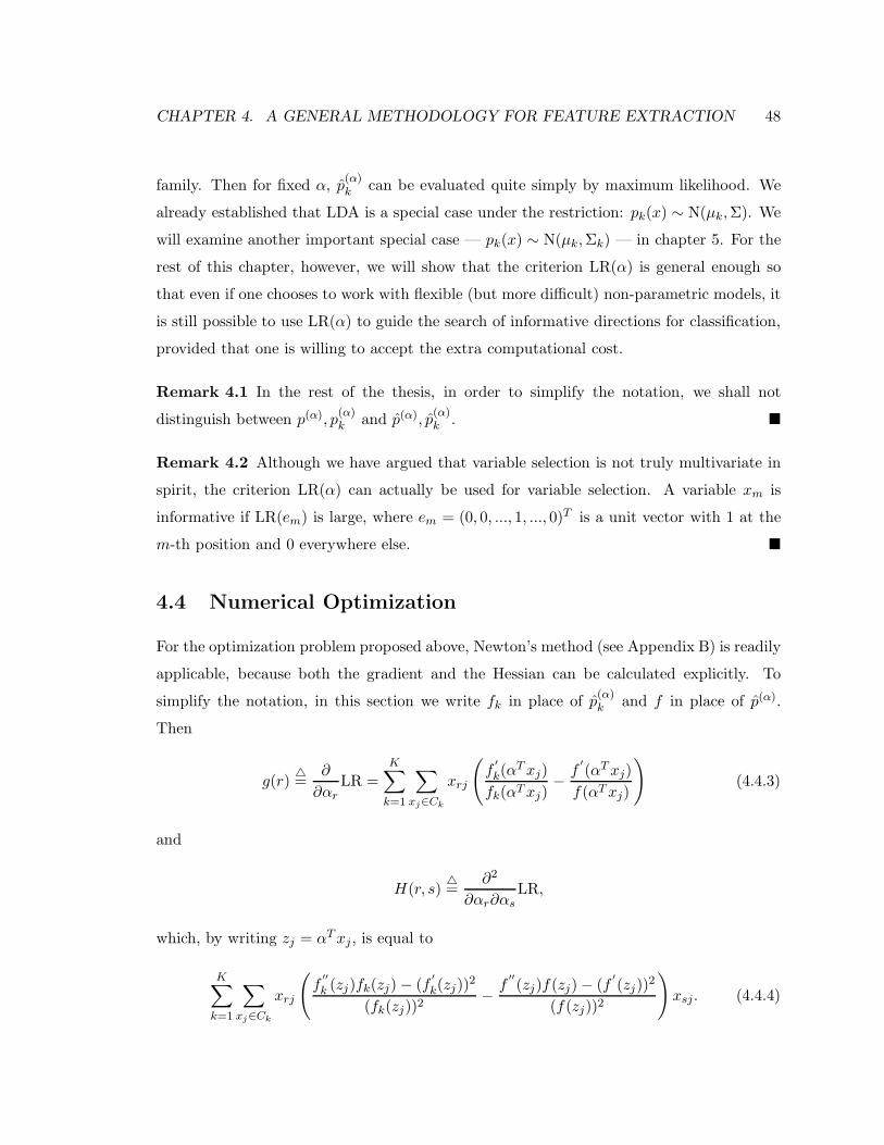
CHAPTER 4. A GENERAL METHODOLOGY FOR FEATURE EXTRACTION 48
family. Then for fixed α, p(α)k can be evaluated quite simply by maximum likelihood. We
already established that LDA is a special case under the restriction: pk(x) ∼ N(µk,Σ). We
will examine another important special case — pk(x) ∼ N(µk,Σk) — in chapter 5. For the
rest of this chapter, however, we will show that the criterion LR(α) is general enough so
that even if one chooses to work with flexible (but more difficult) non-parametric models, it
is still possible to use LR(α) to guide the search of informative directions for classification,
provided that one is willing to accept the extra computational cost.
Remark 4.1 In the rest of the thesis, in order to simplify the notation, we shall not
distinguish between p(α), p(α)k and p(α), p
(α)k .
Remark 4.2 Although we have argued that variable selection is not truly multivariate in
spirit, the criterion LR(α) can actually be used for variable selection. A variable xm is
informative if LR(em) is large, where em = (0, 0, ..., 1, ..., 0)T is a unit vector with 1 at the
m-th position and 0 everywhere else.
4.4 Numerical Optimization
For the optimization problem proposed above, Newton’s method (see Appendix B) is readily
applicable, because both the gradient and the Hessian can be calculated explicitly. To
simplify the notation, in this section we write fk in place of p(α)k and f in place of p(α).
Then
g(r)=
∂
∂αrLR =
K∑
k=1
∑
xj∈Ck
xrj
(
f′
k(αT xj)
fk(αT xj)− f
′
(αT xj)
f(αT xj)
)
(4.4.3)
and
H(r, s)=
∂2
∂αr∂αsLR,
which, by writing zj = αT xj, is equal to
K∑
k=1
∑
xj∈Ck
xrj
(
f′′
k (zj)fk(zj)− (f′
k(zj))2
(fk(zj))2− f
′′
(zj)f(zj)− (f′
(zj))2
(f(zj))2
)
xsj. (4.4.4)

CHAPTER 4. A GENERAL METHODOLOGY FOR FEATURE EXTRACTION 49
Therefore, to estimate g and H, all we need to know is how to estimate a univariate marginal
density and its first two derivatives. This is a relatively easy problem when pk belongs to
a specific parametric family. When pk is modeled non-parametrically, it is also a manage-
able problem (see [36] and Appendix C). We do this once conditionally on each class to
obtain fk, f′
k, f′′
k , and once unconditionally over the entire training sample to obtain f, f′
, f′′
.
There are many different methods for density estimation. Most of them are theoretically
equivalent. Here we only give an outline to the most straight-forward kernel method. Using
a kernel estimator, we can estimate a univariate density as well as its first two derivatives
using the following estimating equations (see e.g., [36]):
f(z) =1
nb1
n∑
i=1
w
(
z − zi
b1
)
,
f′
(z) =1
nb22
n∑
i=1
w′
(
z − zi
b2
)
,
f′′
(z) =1
nb33
n∑
i=1
w′′
(
z − zi
b3
)
,
where w(·) is a kernel density function.
Remark 4.3 In terms of the mean-squared-error criterion for univariate density estimation,
we know the optimal order for choosing the bandwidths, b1, b2, b3, are O(n−1/5), O(n−1/7)
and O(n−1/9), respectively (see e.g., [36]). The choice of the bandwidth parameter has
been an area of intensive research over the past several decades. One might want to be
more particular about the choice of the smoothing parameters, b1, b2, b3, in this problem.
For example, one might argue that the usual mean-squared-error criterion is not the cor-
rect criterion for this problem, since the ultimate goal is not the correct estimation of
the densities per se, but finding the most informative discriminant direction. Thus, one
might be tempted, instead of using the optimal bandwidths for kernel density estimates,
to directly optimize the generalized log-likelihood-ratio criterion, LR(α, b1, b2, b3), over the
smoothing parameters themselves. While we acknowledge such concerns to be reasonable
and well-grounded, we prefer, for the purposes of this thesis, to view the univariate density
estimation problem simply as a separate module for our problem and focus on the most
CHAPTER 4. A GENERAL METHODOLOGY FOR FEATURE EXTRACTION 50
relevant conceptual issues instead.
Remark 4.4 In fact, we prefer to choose bandwidths that are larger than usual, which will
result in over-smoothing. Since the Newton iterates depend heavily on the calculation of
the gradient and the Hessian, it is often desirable to over-smooth the derivatives in order
to avoid numerical instability in the optimization procedure. Note that extremely accurate
estimation of the first two derivatives of the univariate density is not crucial, as long as it
can be ensured that the Newton iterates are generally moving in the correct direction. For
any numerical algorithm to find a meaningful optimum in the objective function, it is much
better to have a smooth function than a wiggly one, or else we get trapped at various local
optima all the time.
Remark 4.5 Every iteration in the numerical optimization routine requires the estimation
of the gradient and the Hessian. Therefore a fast module is needed for non-parametric
density estimation (as well as the derivatives). In our Splus implementation, we use the
Locfit library provided by Clive Loader. More details are in Appendix C and [29].
4.5 Illustration
Therefore the basic feature extraction problem for us is the following optimization problem:
maxα
LR(α).
This is the basis of all numerical procedures in this thesis. In section 4.3, we presented the
theoretical justification for considering such a problem as the basis for feature extraction; in
section 4.4 we presented the heuristics for its numerical implementation. Before we expand
on this basic idea, we illustrate our basic methodology with an example.
Example 6 (Bimodality — Continued) Again, we consider the situation in example 6
(section 2.5), a canonical case where LDA fails. Instead of LDA, we now find the discrim-
inant directions by maximizing LR(α). Figure 4.2 shows the result. The success of LR(α)
is self-evident.

CHAPTER 4. A GENERAL METHODOLOGY FOR FEATURE EXTRACTION 51
Data
0.0 0.2 0.4 0.6 0.8 1.0
0.0
0.2
0.4
0.6
0.8
1.0
1
1
1
1
1
1
1
1
1
1
1
11
1
2
2
2
1
1
11
1
1
2
2
1
2
1
2
1
1
2
2
1
1
1
2
1
1
1
1
2
2
1
2
2
2
1
2
1
1
2
2
1
21
1
1
1
1
1
1
2
2
1
2
1
1
1
2
2
2
1
1
1
2
2
2
2
2
1
1
1
11
1
2
2 1
2
1
1
2
1
1
1
1
22
2
1
1
2
1
2
1
2
1
1
1
1
1
1
1
2
1
2
2 1
1
2
2
1
1
1
2
211
1
21
1
1
2
1
11
1
11
1
1
1
1
2
2
2
2
2 1
1
2
1
1
1
2
2
2
2
1
1
2
1
2
1
1
22
1
2
1
2
2
2
1
1
1
2
1
2
111
1
1
1
1
2
12
1
1
1
2
1
2
2
1
1
2
2 2
11
2
2
1
2
2
1
11
1
2
1
1
2
1 2
2
1
1
1
22
2
12
1
1 1
2
1
1
1
1
2
1
1
1
21
1
1
1
1
2
1
2
1
1
1
1 2
1
1
2
1
1
1
1
1
2
2
1
1
2
1
2
1
1
1
1
1
2
1
1
2
1
2
11
1
1
1
1
12
2
1
2
2
12
11
1
1
1
12
1
1
2
1
1
1
11
2
1
1
1
2
1
12
2
2
2
1
2
1
2
1
1
2
2
2
1
1
22
1
2
2
1
1
1
1
1
12
1
1
1
2
2
1
1
1
11
2
11
2
1
1
1
1
1
21
1
1
1
1
2
2
2
2
2
1
2
2
1
2
11
21
1
2
2
1
2
2
1
2
2
1
1
1
1
1
2
2
2
1
1
2
1
2
2
1
1
2
2
22
1
1
1
2
1
2
1
1
11
1
2
2
12
12
2
1
1
2
1
1
1
2
2
2
1
1
2
2
2
1
12
21
2
2
1
1
1
2
1
2
2
2
2
1
1
1
1
2
2 1
1
1
2
2
2
1
1
1
11
2
2
1
2
1
1
1
2
1
1
1
1
2
21
2
1
2
1
2
1
1
2
0.0 0.2 0.4 0.6 0.8 1.0
020
4060
80
LR
Figure 4.2: Left: The horizontal axis is the best discriminant direction for this case. Right:Histogram (100 simulations) of cos(θ), where θ is the acute angle formed between the hor-izontal axis and the discriminant direction resulting from maximizing LR(α). We recoverthe correct direction most of the time.
Remark 4.6 Figure 4.2 shows that our procedure still produces wrong directions occa-
sionally. This reflects the existence of local maxima in some simulations. The existence of
local maxima is relative to the bandwidth we select. With a larger bandwidth, the objec-
tive function becomes smoother, and it is less likely for the procedure to be trapped at a
local maximum. In our simulation, we’ve used a common bandwidth for every realization.
Apparently this bandwidth is not appropriate for every single realization. This also reflects
the inherent difficulty in numerical optimization. One solution to avoid local maximum in
practice is to take large steps in the beginning to get into a local neighborhood of the true
maximum and use Newton steps only in the local neighborhood. This strategy is adopted,
for example, by Friedman in exploratory projection pursuit [11]. We will come back to
projection pursuit later.
4.6 Finding Multiple Features
Fisher’s LDA finds more than one discriminant direction. Since it is an eigen-decomposition
problem, one usually goes beyond the first eigenvector to consider a few more eigenvectors
(of decreasing importance). How, then, should one go about finding subsequent directions
when our new problem is no longer an eigen-decomposition problem? Here we investigate
several possibilities.
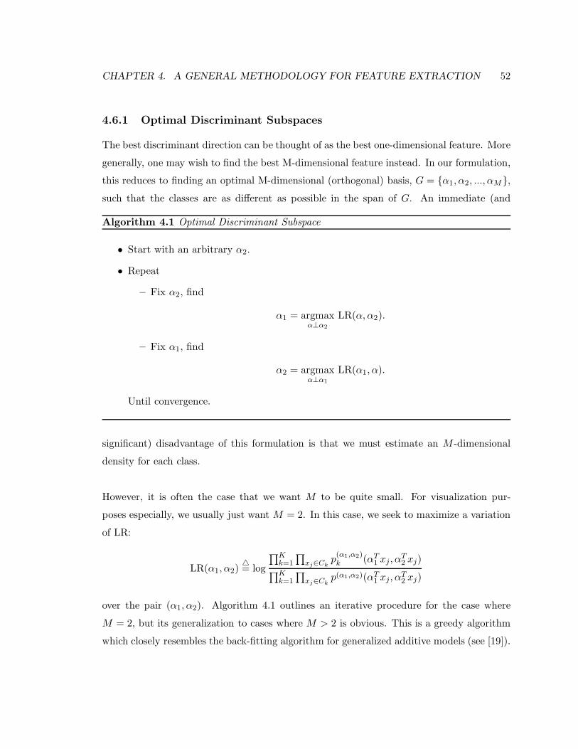
CHAPTER 4. A GENERAL METHODOLOGY FOR FEATURE EXTRACTION 52
4.6.1 Optimal Discriminant Subspaces
The best discriminant direction can be thought of as the best one-dimensional feature. More
generally, one may wish to find the best M-dimensional feature instead. In our formulation,
this reduces to finding an optimal M-dimensional (orthogonal) basis, G = α1, α2, ..., αM,such that the classes are as different as possible in the span of G. An immediate (and
Algorithm 4.1 Optimal Discriminant Subspace
• Start with an arbitrary α2.
• Repeat
– Fix α2, find
α1 = argmaxα⊥α2
LR(α,α2).
– Fix α1, find
α2 = argmaxα⊥α1
LR(α1, α).
Until convergence.
significant) disadvantage of this formulation is that we must estimate an M -dimensional
density for each class.
However, it is often the case that we want M to be quite small. For visualization pur-
poses especially, we usually just want M = 2. In this case, we seek to maximize a variation
of LR:
LR(α1, α2)= log
∏Kk=1
∏
xj∈Ckp(α1,α2)k (αT
1 xj, αT2 xj)
∏Kk=1
∏
xj∈Ckp(α1,α2)(αT
1 xj, αT2 xj)
over the pair (α1, α2). Algorithm 4.1 outlines an iterative procedure for the case where
M = 2, but its generalization to cases where M > 2 is obvious. This is a greedy algorithm
which closely resembles the back-fitting algorithm for generalized additive models (see [19]).

CHAPTER 4. A GENERAL METHODOLOGY FOR FEATURE EXTRACTION 53
4.6.2 Sequence of Nested Discriminant Subspaces
We can simplify the computation considerably if we restrict our attention only to a sequence
of nested subspaces; that is, we force the best m-dimensional discriminant subspace to
contain the best (m−1)-dimensional subspace (algorithm 4.2). For M = 2, we can see that
Algorithm 4.2 Nested Discriminant Subspaces
• Find the optimal 1-dimensional discriminant subspace
α1 = argmaxα
LR(α).
• For m = 2 to M :
– Let spanα1, α2, ..., αm−1 be the (m− 1)-dimensional discriminant subspace.
– Find
αm = argmaxα⊥αj ,j<m
LR(α1, α2, ..., αm−1, α)
EndFor
this is a much simplified version of algorithm 4.1. It terminates in one step without the
back-fitting loop and, therefore, reduces the computation by a significant amount. But for
moderately large M , we are still “cursed,” since we still have to estimate density functions
in M dimensions.
4.6.3 Orthogonal Features
To avoid estimating multivariate densities, one can use an even cruder approximation (see
algorithm 4.3), where we focus only on 1-dimensional features and simply force all the fea-
tures to be orthogonal. This is a very practical algorithm, because it requires very little
effort to go beyond the first feature. The orthogonality constraint is not entirely unreason-
able and is, in fact, standard practice in multivariate statistics, e.g., principal component
analysis, etc.

CHAPTER 4. A GENERAL METHODOLOGY FOR FEATURE EXTRACTION 54
Algorithm 4.3 Orthogonal Feature Extraction
• Find
α1 = argmaxα
LR(α).
• For m = 2 to M :
– Orthogonalization: Let P be a projection operator that projects x ontospanα1, α2, ..., αm−1. That is, if Q is a matrix that stacks αj , j = 1, 2, ...,m−1as column vectors, then
P = Q(QT Q)−1QT ,
and let
x←− (I − P )x.
– Find
αm = argmaxα
LR(α).
EndFor

CHAPTER 4. A GENERAL METHODOLOGY FOR FEATURE EXTRACTION 55
However, in classical multivariate statistics, one often assumes that the data follow a multi-
dimensional Gaussian distribution, so there is a natural coordinate system in which it is
interesting and meaningful to focus on features that are orthogonal to one another. In
particular, if x ∼ N(µ,Σ), then it is natural to sphere the data, i.e., let x∗ = Σ−1/2x, and
consider orthogonal directions in the transformed space. In terms of the original space, αj
and αm are orthogonal if αTj Σαm = 0. Sometimes, we say that they are orthogonal with
respect to the metric Σ.
For non-Gaussian data, no such natural metric exists. In fact, for data separated into
K classes, even if we assume that the data in each class are Gaussian, it is still not clear
what the appropriate metric is, unless one assumes, as in LDA, that all the classes share
a common covariance matrix. In practice, one often spheres the data prior to the analysis.
This is the same as using the total covariance matrix as an ad-hoc metric for orthogonal-
ization.
In general, there is no reason why the total covariance matrix is the appropriate metric. In
the next section, we focus on a strategy that does not use orthogonality as a constraint on
the subsequent directions. Before we proceed with the details, we feel it is important to add
that orthogonal features are still useful for some applications, such as data visualization,
despite its ad-hoc-ness.
4.7 Non-orthogonal Features
Whether it is subspace optimization or searching for directions one at a time, the algo-
rithms we’ve presented so far can find as many features as the dimensionality of the data.
This alone is an important improvement over Fisher’s LDA. Recall the between-class co-
variance matrix has at the most min(K − 1, d) non-trivial eigenvectors and it is often the
case that K ≪ d. Although our goal is dimension reduction, it may be undesirable for
high-dimensional problems to have the number of discriminant directions be restricted by
the total number of classes, K (usually quite small), especially when the class densities
are, for example, multi-modal. Consider a 2-class problem (K = 2) in d = 100 dimension.

CHAPTER 4. A GENERAL METHODOLOGY FOR FEATURE EXTRACTION 56
While for classification it is probably not necessary to use 100 discriminant directions, we
may nevertheless need to use a few more directions than just one (K − 1 = 2− 1 = 1). On
the other hand, we are usually not concerned with being unable to extract more features
than the dimensionality of the data. After all, our goal is dimension reduction!
The reason we can’t find more features than the dimensionality of the data is that the
informative features are always constrained to be orthogonal to one another. This is a more
serious problem, due to the unavoidable ad-hoc-ness in choosing a proper metric, as we in-
dicated in section 4.6.3. One systematic way to find non-orthogonal features is to eliminate
all previously discovered features in the data before proceeding to search for new features.
4.7.1 Exploratory Projection Pursuit
The feature extraction problem can be viewed as an exploratory projection pursuit problem.
Algorithm 4.4 provides a generic exploratory projection pursuit procedure, first proposed
by Friedman in [11]. Step (1) is simply a numerical optimization step. Step (2) needs
Algorithm 4.4 Exploratory Projection Pursuit
• Repeat
(1) Find α = argmax I(α), where I(α) is a (problem-specific) projection index whichis large for directions with interesting features.
(2) Transform the data
x←− h(x)
so that the projection index reaches its minimum along α, without changing xin all directions orthogonal to α.
• Stop when no interesting features can be found.
some further clarification. In [11], the projection index I(α) is taken to be a measure of
deviation from normality, and directions are chosen to maximize this measure. Hence the
procedure seeks the most non-Gaussian direction in the data. In this context, step (2)
means to transform the data so that its marginal distribution along α is exactly Gaussian.

CHAPTER 4. A GENERAL METHODOLOGY FOR FEATURE EXTRACTION 57
In particular, let z = αTx, then a transformation is incurred on z:
z′ = Φ−1(Fz(z))= γ(z),
where Φ(·) is the standard Gaussian cdf and Fz is the marginal cdf of z, so that γ(·) is a
monotonic one-to-one transformation and z′ has a standard Gaussian distribution. Let A
be an orthogonal rotation matrix such that
z= Ax =
αTx
A∗x
, (4.7.5)
which can be constructed using the Gram-Schmidt procedure (e.g., page 307 of [10]). Then
the entire transformation process can be summarized in the following diagram:
xh−−−→ h(x)
yA
x
A−1
zt−−−→ t(z)
(4.7.6)
where
t(zj) =
γ(zj) for j = 1,
zj for j > 1.(4.7.7)
Hence
h(x) = A−1t(Ax).
Remark 4.7 Theoretically speaking, when a transformation is incurred to remove the in-
teresting features in α2, one might introduce some additional features back in α1. Friedman
states in [11] that this is not a serious problem in practice and does not warrant any deep
concern.

CHAPTER 4. A GENERAL METHODOLOGY FOR FEATURE EXTRACTION 58
4.7.2 Finding Non-orthogonal Features via Feature Removal
The exploratory projection pursuit algorithm can be easily adapted to fit our feature ex-
traction problem (algorithm 4.5). We simply use LR(α) as the projection index. Again,
Algorithm 4.5 Non-Orthogonal Feature Extraction via Feature Removal
• Repeat
(1) Find the most informative feature in the data, α = argmax LR(α), the optimaldiscrimininant direction.
(2) Transform the data
x←− h(x)
so that the direction α contains the least informative feature, i.e., so that thereis no class separation in the α direction.
• Stop when the classes are more or less the same along all directions.
we must be more specific about step (2). What does it mean to say that there is no class
separation along α? It means the marginal density along α must be the same for all classes,
i.e., p(α)k (·) = p(α)(·) for some common p(α)(·). Since we are free to specify this common
density, we might just as well choose p(α)(·) = g(·), the standard Gaussian, for simplicity.
Hence h(x) remains the same as in equation (4.7.6).
This algorithm is also very practical. The transformation h(·) involves only an orthogo-
nal rotation and a one-dimensional monotonic transformation. To add to the theoretical
consistency of our presentation, we present a result that relates this procedure to the clas-
sical LDA.
Result 4.2 If pk(x) = N(µk,Σ) for class k, then algorithm 4.5 yields the same discriminant
directions as LDA.
Proof Since x ∼ N(µk,Σ) for class k, result 4.1 tells us that in this special case, our

CHAPTER 4. A GENERAL METHODOLOGY FOR FEATURE EXTRACTION 59
projection index, LR(α), is equivalent to
αT Bα
αT Wα.
We now proceed in three steps:
1. Without loss of generality, we assume that Σ = I, so that W is also identity. For
arbitrary Σ, this can be achieved by a simple transformation Σ−1/2x. Let B be
the between-class covariance matrix as usual. Without loss of generality, we further
assume that the first eigenvector of B is α = (1, 0, 0, ..., 0)T . Although this is usually
not the case, we can always apply an orthogonal rotation so that it is. Now, by
definition we have Bα = λ1α. We then partition B so that B11 is a scalar and get
B11 B12
B21 B22
1
0
=
B11
B21
=
λ1
0
which implies that B11 = λ1 and B21 = BT12 = 0, where 0 = (0, 0, ..., 0)T is a vector
of zeros. This implies that the matrix B has a special block-diagonal form:
B =
λ1 0T
0 B22
and λ1 is its largest eigenvalue.
2. Now consider LDA in this simple setting. The best discriminant direction is the first
eigenvector of B, α. The next best discriminant direction is the second eigenvector
of B, call it β. Due to the special form of the matrix B, it is easy to verify that its
second eigenvector must have the following form:
β =
0
β2
,
where β2 is the first eigenvector of B22. To be more specific, note that β is constrained
to be orthogonal to α. Since α = (1, 0, 0, ..., 0)T , this means the first element of β
CHAPTER 4. A GENERAL METHODOLOGY FOR FEATURE EXTRACTION 60
must be 0 and we have Bβ = λ2β, or
λ1 0T
0 B22
0
β2
=
0
B22β2
=
0
λ2β2
.
That is, β2 is an eigenvector of B22. But λ2, being the second largest eigenvalue of B,
is clearly the largest eigenvalue of B22. So β2 is, in fact, the first eigenvector of B22.
3. In the exploratory projection pursuit procedure, after the best discriminant direction
α has been identified, the transformation γk(·) is applied in that direction to class
k. In our simple setting, γk(·) is simply applied to the first coordinate, x1. Since
x1 ∼ N(µk,1, 1),
γk(x1) = Φ−1(Fx1(x1))
= x1 − µk,1
is simply a location shift. Therefore, after the transformation the new between-class
covariance has the following form:
B∗ =
0 0T
0 B22
since the class means have been made identically 0 for all classes in the first coordinate
but have stayed the same in all other coordinates. Furthermore, the location shift γk(·)does not change W , the within-class covariance. The next best discriminant direction
is simply the first eigenvector of B∗. Let β∗ be such a vector; the special form of B∗
implies immediately that
β∗ =
0
β∗2
,
where β∗2 is the first eigenvector of B22. This establishes that β∗ is the same as β.
Such an argument can be carried out repeatedly. Once the first two directions have been
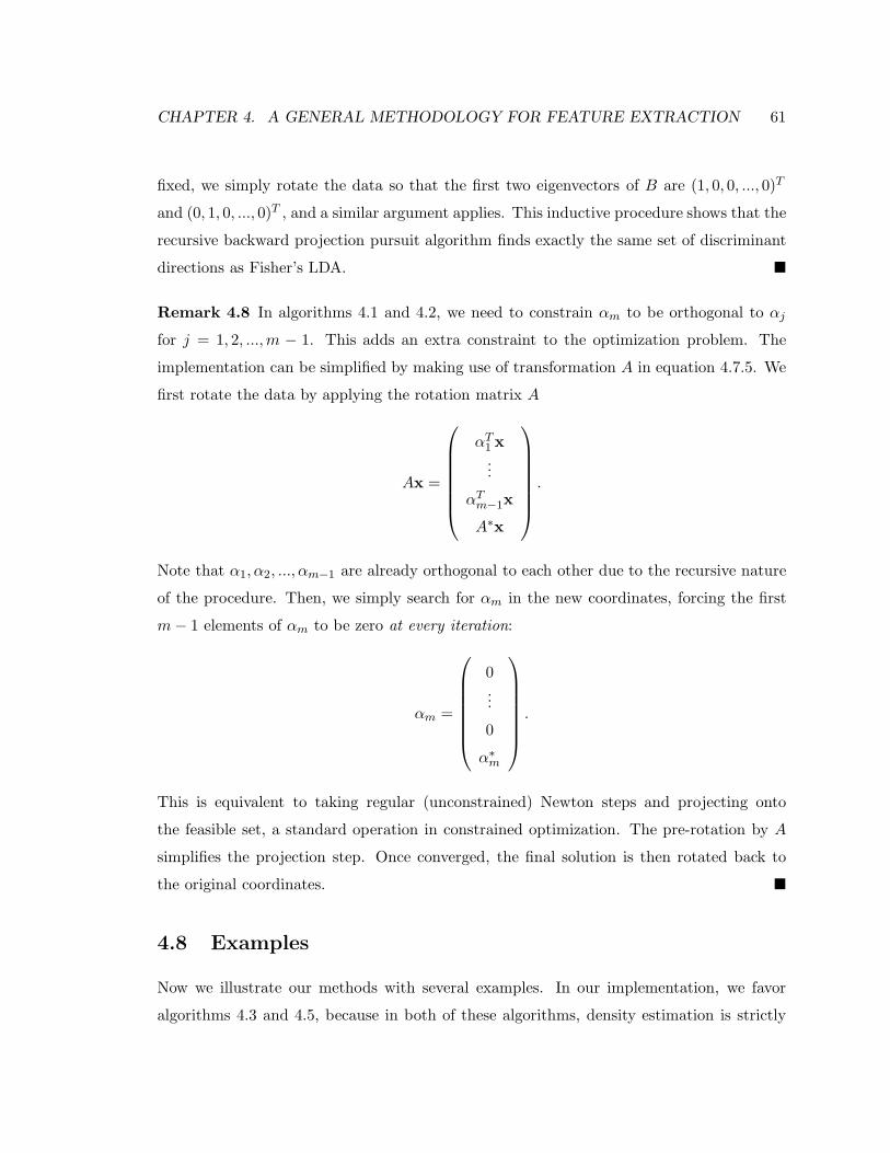
CHAPTER 4. A GENERAL METHODOLOGY FOR FEATURE EXTRACTION 61
fixed, we simply rotate the data so that the first two eigenvectors of B are (1, 0, 0, ..., 0)T
and (0, 1, 0, ..., 0)T , and a similar argument applies. This inductive procedure shows that the
recursive backward projection pursuit algorithm finds exactly the same set of discriminant
directions as Fisher’s LDA.
Remark 4.8 In algorithms 4.1 and 4.2, we need to constrain αm to be orthogonal to αj
for j = 1, 2, ...,m − 1. This adds an extra constraint to the optimization problem. The
implementation can be simplified by making use of transformation A in equation 4.7.5. We
first rotate the data by applying the rotation matrix A
Ax =
αT1 x...
αTm−1x
A∗x
.
Note that α1, α2, ..., αm−1 are already orthogonal to each other due to the recursive nature
of the procedure. Then, we simply search for αm in the new coordinates, forcing the first
m− 1 elements of αm to be zero at every iteration:
αm =
0...
0
α∗m
.
This is equivalent to taking regular (unconstrained) Newton steps and projecting onto
the feasible set, a standard operation in constrained optimization. The pre-rotation by A
simplifies the projection step. Once converged, the final solution is then rotated back to
the original coordinates.
4.8 Examples
Now we illustrate our methods with several examples. In our implementation, we favor
algorithms 4.3 and 4.5, because in both of these algorithms, density estimation is strictly
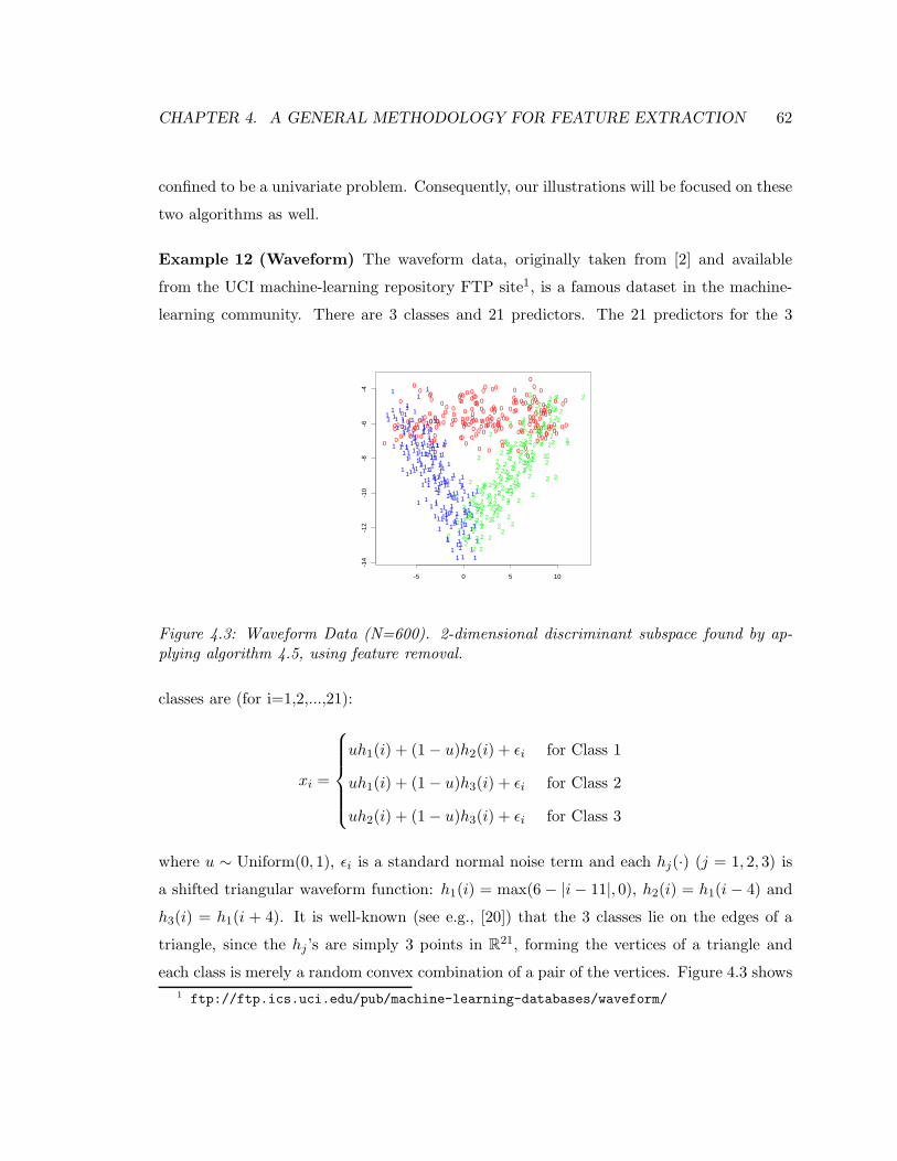
CHAPTER 4. A GENERAL METHODOLOGY FOR FEATURE EXTRACTION 62
confined to be a univariate problem. Consequently, our illustrations will be focused on these
two algorithms as well.
Example 12 (Waveform) The waveform data, originally taken from [2] and available
from the UCI machine-learning repository FTP site1, is a famous dataset in the machine-
learning community. There are 3 classes and 21 predictors. The 21 predictors for the 3
-5 0 5 10
-14
-12
-10
-8-6
-4
2
22
2
0
2
0 0
01 0
2
2
0
2
0
1
1
2
2
1
2
0
2
0
1
1
2
1
2
0
0
1
0
1
1
2
1
2
2
0
2
2
0
2
2
1
0
2
1
1
0
2
0
1
2
02
0
1
0
2
1 11
2
1
0
1
0
0
2
21
1
1
11
1
2
1
1
2
1
0
0
2
1
2
0
2
1
0
2
0
2
0
21
2
1
0
1
12
0 0
1
1
0
2
2
2
1
1
12
0
2
0
2
1
0
1
2
1
1
2
2
0
0
211
0
0
0
2
0
2
2
0 0
2
2
0
0 0
1
1
2
1
1
1
2
0
2
0
2
0
2
2
0
0 0
2
1
0 0 0
0
2
2
1
1
2
1
2
2
2
0
0
2
0
0
12
0
11
22
2
0
2
1
0
1
0
1
1
0
1
21
0
2
1
2
11
0
0 0
1
2
1
0
0
2
2
2
1
2
0
1
2
1
1
0
1 0
1
1
1 2 2
2
0
2
0
2
2
0
0
0
1
2
2 0
1
0
1 0
0
2
1
0
0
1
1
0 0
1
0
1
2
2
1
0
2
1
0
2
2
1
0
1
2
1
0 0
1
1
2
2
0
0
2
0
0
1
2
0
1
2
02 0
2
02
0
2
2
0
0 0
0
1
0
1
2
1
1
0
01
1
1
2
22
0
21
0
2 0
0
2
0
1
2
0
1
0
0
221
2
1
0
1
0
1
1
2
0
2
0
1
1
1
1
0
2
1
0 0
2
2
0 0
0
11
2
2
2
1
2
1
0
2
0 02
0 0
2
1
0
2
1
2
2
0
1
2 2 0
1
1
0 0
1
2
0
1
0 0
1
1
01
2
1
0
0
21
2
2
0
0
0
2
1
2
2
22
1
0
1 22
1
1
2
0
2
2 0
2
0
1
2
1
0
1
2
1
2
1
0
1
2
1
0
1
0
1
1 2
2
1
2
2
0
1
0
2
2
0 01 0
1
0
1 0 0
2
1 02
1
0
11
1
2
1
0
0
2
1
0
2
0
2
0
2
1
0
01 0
01
2
2
1
2
1
1
2
2
11
2
21
0
1
2
2
1
1
0
0
2
0
22
2
1 0
2
0
1
2
2
0
2
1
1
0
1
0
1
0
1
2
1
1
0
2
0
0
1
11
1
2
1
1
1
21
0
2
1
1 1
0
22
1
22
1
2
1
0
1
2
2
01
22
0
1
2
0
2
0 0
1 22
0
1
1
0
1
Figure 4.3: Waveform Data (N=600). 2-dimensional discriminant subspace found by ap-plying algorithm 4.5, using feature removal.
classes are (for i=1,2,...,21):
xi =
uh1(i) + (1− u)h2(i) + ǫi for Class 1
uh1(i) + (1− u)h3(i) + ǫi for Class 2
uh2(i) + (1− u)h3(i) + ǫi for Class 3
where u ∼ Uniform(0, 1), ǫi is a standard normal noise term and each hj(·) (j = 1, 2, 3) is
a shifted triangular waveform function: h1(i) = max(6 − |i− 11|, 0), h2(i) = h1(i − 4) and
h3(i) = h1(i + 4). It is well-known (see e.g., [20]) that the 3 classes lie on the edges of a
triangle, since the hj ’s are simply 3 points in R21, forming the vertices of a triangle and
each class is merely a random convex combination of a pair of the vertices. Figure 4.3 shows
1 ftp://ftp.ics.uci.edu/pub/machine-learning-databases/waveform/
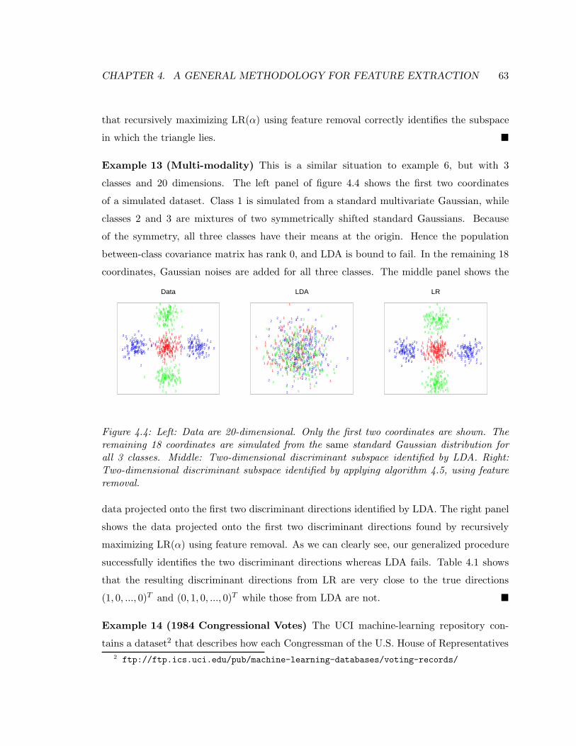
CHAPTER 4. A GENERAL METHODOLOGY FOR FEATURE EXTRACTION 63
that recursively maximizing LR(α) using feature removal correctly identifies the subspace
in which the triangle lies.
Example 13 (Multi-modality) This is a similar situation to example 6, but with 3
classes and 20 dimensions. The left panel of figure 4.4 shows the first two coordinates
of a simulated dataset. Class 1 is simulated from a standard multivariate Gaussian, while
classes 2 and 3 are mixtures of two symmetrically shifted standard Gaussians. Because
of the symmetry, all three classes have their means at the origin. Hence the population
between-class covariance matrix has rank 0, and LDA is bound to fail. In the remaining 18
coordinates, Gaussian noises are added for all three classes. The middle panel shows the
Data
11111
1
1
1 11
1
1
1
11
1
1
1
1 1
1
1
11
1
1
1
1
1
1
11
1
1
1
11
11
11
1
1
1
1
11 1
1
111
11
1
11
1
1
11
1
111
1
1
1
11
1
1
1
11 111
11
1
1
1
1 1
1
11 1 1
111
1
1
11 1
1
1
1
1
1 1
1
1
1 11
1
11 1
11
1
1
1
1
1
1
1 111
1
1
1
1
1
1
1
1
1
1
111
111
1
111 1
1 1
1
11
1
1
1
1
11 1
1
1
1
1
1
1
1
1
1
1 1
1
1
111
1 1 111
11
1
11
1
11
1
1
1
1
1
11
11
11
1
1
2 22
2222
2
2
2
22
2
2 22 2
2
22
2
22
2
22 2
2
22
2
2
22
2
2
2
2
2 2
2
2
2
222 2
2
2
2
2 2
222
22 2
2
2
2
2
2
2
2
2
222
2
2
2
2
2
2
2222
2
22 2
2
2
2
22
22 22 2
2
22
222
222
2
2
22
2
2
2
2
2
22
222
2
2
2 2
2
2
2
2 2
2
2
2
222
2
22
222
2
2
2
2
222
2
222
2
222
2
22
2 2
2
2
2 22
2
222
222
22
2
2
2
2
2
2
2
2
2
2
22
2 2
22 2
22
2
2
22
22
22
2
2
3
3
33
3
33
3333
3
3
3
3
3 3
3
3
3
3
3
3
3
3
3
333
3
3
33
333
3
33
3
3
3
3
33
3
3
33
3
33
3
33
33
33 3
3
3
333
3
33
3
3
3
33
3
3
3
33 3
3
3
3
3
3
3
33
33
3
33
3
33
3
3
3
3
3
3
3
3
3 3333
3
3
3 3
3
33
3
3
33
33 3
3
3
3
3
3
3
3
3
3
3
3 3
3
3333
333
3
33
3
33
3
3
3
3
3
3
3
33
3
333
3
3
33 3 3 33
3
3
3 3
3
3
3
33
3 3
3
3
33
33
3
33
3 3
3 3
3
3
3
3
3
33
LDA
1
1
11
11
1
1
1
111
1
11
1
1
1
1
1
1
1
1
11
1
1
1
1
1
1
1
1
1
1
1
1
1
1
1
1
1
1
1
1
1
1
1
1
1
11
11
1
11
1
1
1
11
1
1
1
1
1
1
11
1
1 1
11
11
11
1
1
1
1
1
1
1
1
1
1
11
1
1
1
1
1
1 1
1
1
1
11
1
1
1
1
1
1
1
1
1
1
1
1
1
1
11
11
1
1
1
1
1
1
1
1
1
1
1
1
1
1
1
1
1
11
1
1
1
1
1
1
1
1
1
1
1
1
1
1
1
1
1
1
11
1
1
11
1
1
1
1 1
1
1
11
1
11
1
1
1
1
11
11
1
1
1
1
1
1
1
1
1
1
1
1
1
1
11
2
2
2
2
2
2
2
2
2
2
2
2
2
2
2
22
2
2 2
2
2
2
2 2
2
2
2
2
2
2
2
2
2
2
2
2
2
2
22
2
2
2
2
2
2
22
2
2
22
22
2
2
2
2
22
2
2
2
2
2
2
22
2
2
2
2
2
22
2
2
2
2
2
2
22 2
22
2
2
2
2
22
2
2
2
2
2
2
2
2
2
2
2
2
2
2
2
2
2
22
22
2
2
2
2
2
2
22
2
2
2
2
2
2 2
2
2
2
2
2
2
2
2
2
22
2
2
2
2
2
2
2
2
2
2
2 2
2
2
2
2
2
2
2
2
22
2
2
2
2
22
2
2
2
2
2
2
2
2
2
2
2 2
2
22
2
2
2
2
2
2
2
2
2
2
2
2
2
2
2
2
2
33
3
333
3
3
3
3
3
333
3
3
3
3 3
3
3
3
3
3
3
3
3
333
3
33 3
3
33
3
3
3
3
3
3
33
3
33
33
3
3
3
3
3
3
3
33
3
333
33
3
3
3
3
3
3
3
3
33
3
3
3
3
3
3
3
3
3
3
3
3
3
3
3
3
3
3
3
33
3
3
33
3
3
3
3 3
3
3
3
3
3
3
3
3
3
3
3
33
3
3
3
3
33
3 3
3
3
3
33
3
3
3
3
3
3
3
3
3
3
3
3
3
3
3
3 3
3
3
3
3
3
3
3
33
3
3
3
3
3
3
33
3
3
3
333
3
3
3
3
3
3 3
3
3
3
3
3
3
3
3
3
3
3
3
3
3
3 33
3
3
3
3
3
LR
111
111
11
11
1
1
1
11 1
1
1
11
1
1
111
1
1
1
1
1
11
1
1
1
11
11
11
1
1
1
1
11
1
1
111
11
1
11
1
1
111
1 11
1
1
1
11
1
1
1
111 11
11
1
1
1
11
1
111
1
1
11
1
1
1 11
1
1
1
111
1
1
11
1
1
1 11
111
1
1
11
1
1111
11
1
1
1
1
1
1
1
1
1
11
1 11
1
1
1
11
111
11
1
1
1
1
1
11
1
1
1
1
1
11
1
1
11
1
1
111
11
11 1
1 1
1
1
1
1
11
1
1
1
11
11
11
11
1
1
2
2 2
2
222
2
22
2 22
22222
2 22
2 2
2
2 22
2
2
2
22
2
2
2
2
2
2
22
2
2
222
22
2
2
2
22
22 2
22
2
2
2
2
2
2
2
2
2
2 2
2
2
2
2
2
2
2
2 2 2 2
2
2
22
2
2
2
222 2
2 22
222
2 222
2 2
2
2
2
2
2
2
2
2
2
2
2
2 22
2
2
22
2
22
22
2
2
2
22
2
2
2 2
22
22
2
22
222
2
2 22
2
2 22
2
22
22
2
2
22
2
2
222
2
22
22
2
2
2
2
2
2
2
2
2
2
22
22
2 222
2
2
2
22
2 22 2
22
3
3
33
3
33
333
33
3
3
3
333
3
3
33
3
3
3
3
33 3
3
3
33
33 3
3
3
33
3
3
33
33
3
33
3
33
3
333
3
333
3
3
33 3
3
3
3
3
3
3
33
3
3
3
33
3
33
33
3
3
33
3
3
3
33
3
33
3
3
3
3
3
3
3
3
3333
3
3
3
33
33 3
3
3
33
333
3
3
3
3
3
3
3
3
3
3
33
3
33
3 3333
3
333
3
3
3
3
3
3
3
3
3
33
3
33 3
3
3
3 33
33
3
3
3
33
3
3
3
33
33
3
3
3 3
3
3
3
33
33
33
3
3
3
3
3
3
3
Figure 4.4: Left: Data are 20-dimensional. Only the first two coordinates are shown. Theremaining 18 coordinates are simulated from the same standard Gaussian distribution forall 3 classes. Middle: Two-dimensional discriminant subspace identified by LDA. Right:Two-dimensional discriminant subspace identified by applying algorithm 4.5, using featureremoval.
data projected onto the first two discriminant directions identified by LDA. The right panel
shows the data projected onto the first two discriminant directions found by recursively
maximizing LR(α) using feature removal. As we can clearly see, our generalized procedure
successfully identifies the two discriminant directions whereas LDA fails. Table 4.1 shows
that the resulting discriminant directions from LR are very close to the true directions
(1, 0, ..., 0)T and (0, 1, 0, ..., 0)T while those from LDA are not.
Example 14 (1984 Congressional Votes) The UCI machine-learning repository con-
tains a dataset2 that describes how each Congressman of the U.S. House of Representatives2 ftp://ftp.ics.uci.edu/pub/machine-learning-databases/voting-records/
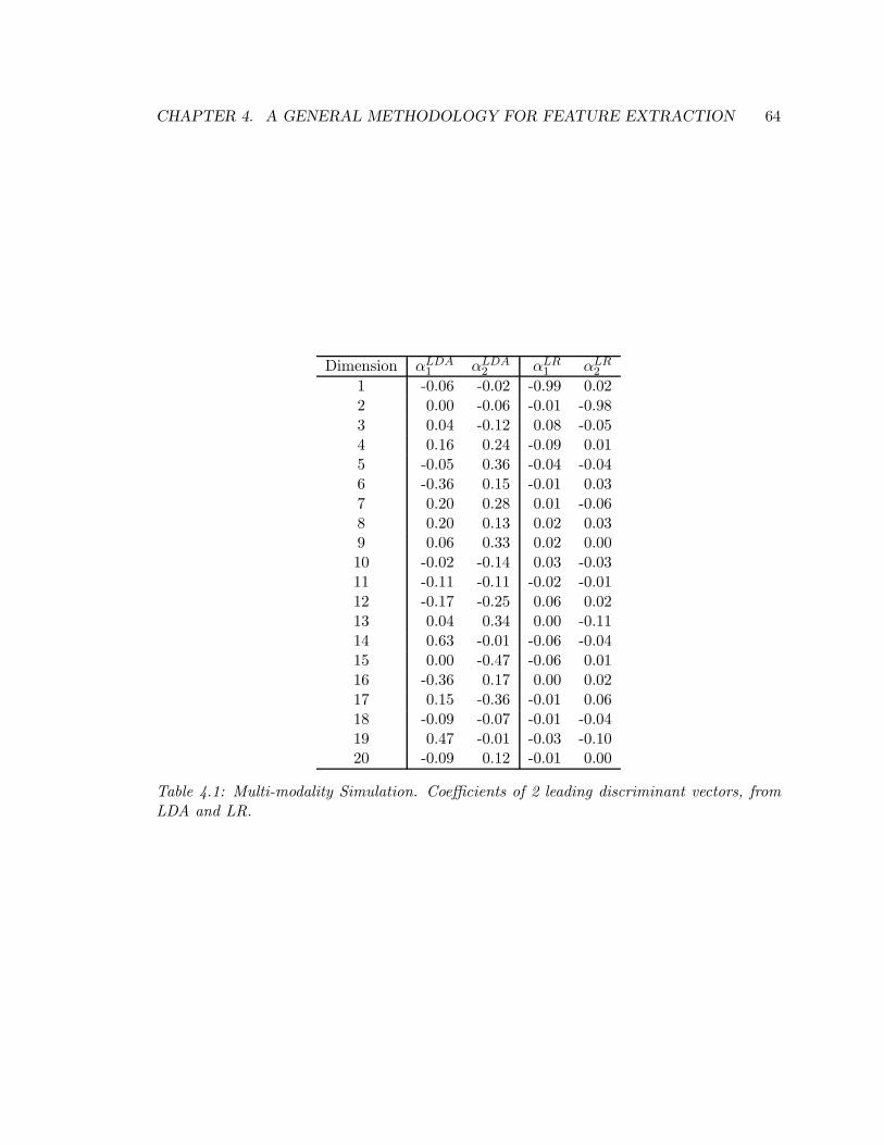
CHAPTER 4. A GENERAL METHODOLOGY FOR FEATURE EXTRACTION 64
Dimension αLDA1 αLDA
2 αLR1 αLR
2
1 -0.06 -0.02 -0.99 0.022 0.00 -0.06 -0.01 -0.983 0.04 -0.12 0.08 -0.054 0.16 0.24 -0.09 0.015 -0.05 0.36 -0.04 -0.046 -0.36 0.15 -0.01 0.037 0.20 0.28 0.01 -0.068 0.20 0.13 0.02 0.039 0.06 0.33 0.02 0.0010 -0.02 -0.14 0.03 -0.0311 -0.11 -0.11 -0.02 -0.0112 -0.17 -0.25 0.06 0.0213 0.04 0.34 0.00 -0.1114 0.63 -0.01 -0.06 -0.0415 0.00 -0.47 -0.06 0.0116 -0.36 0.17 0.00 0.0217 0.15 -0.36 -0.01 0.0618 -0.09 -0.07 -0.01 -0.0419 0.47 -0.01 -0.03 -0.1020 -0.09 0.12 -0.01 0.00
Table 4.1: Multi-modality Simulation. Coefficients of 2 leading discriminant vectors, fromLDA and LR.

CHAPTER 4. A GENERAL METHODOLOGY FOR FEATURE EXTRACTION 65
voted on 16 key issues in 1984. There are 435 Congressmen in the original database, of which
232 (124 Democrats and 108 Republicans) have a complete record (with a clear “yes” or
“no” vote recorded on all 16 issues). In the case where a Congressman’s vote on a certain
LDA
0 2 4 6
-20
24
d
rd
dd
dd
r
dr
d
rd r
r
rddd
ddd
rrr
rrrdrr
rd
r
r
dd
d
d
r
rr
d
rr
d
dd
d
d
d
d
d
d
dr
d
dr
d r r
d
rrr
dd
r
r
r
d
r
d
r
dd
rrr
dd
d
r
rr
d
d
d
r
ddddddd
dd
d
d
r
d
rd
d
rd
d
r
r
d
r
d r
rrr
rd
d
r
d
ddrr
d
r
d
d
r
d ddd
r
r
dd
r
r
r
r
rd
r
d
d
dd r
d
d
r
rr
rr
rd r
d
d
r
r
d
d
d
d
r
d
rdrd
dd
rr
r
d
rr
r
r
d
r
r
r
rr
dd
r
r
d
drr
d rr
d
d
d
d
r
d
d
rrr
d
dr
r
d
rd
r
d
d
d
r
d
dd
d
r
r
d
LR
-0.2 0.0 0.2 0.4 0.6 0.8 1.0 1.20.
00.
51.
0
d
r
d
dd
dd
r
d
r
d
r
d
r
rr
d
ddd
d
d
r
rr
rrr
d
r
rr
d
r
r
d
d
d
d
rrr
d
rr
d
d
dd
d
d
d
d
d
d
r
dd
rdr
r
d
rr
r
d
d
r
rr
d
r
d
rd
d
r
r
r
d
d
d
rr
r
d
d
dr
d
ddd
d
d
d
d
d
d
d
r
d
r
d
d
r
d
d rr
d
r
d
r rrr
r
d
d
r
d
d
d
rr
d
r
d
d
rd
ddd
r
r
dd
rrrrr
d
r
d
d
dd
r
d
d
rrrr
rr
d
r
d
d
rr
d
d
d
d
r
d
r
d
r
dd
d
rrr
dr
rrr
d
rr
r
rr
dd
r
r
d
d
r
rd
rr
dd
d
d
r
d
d
r
rr
d
d
r
r
d
r
d
r
d
dd
r
d
d
d
d
r
r
d
Figure 4.5: Congressional Votes Data. Left: Two-dimensional subspace identified by LDA— the second direction is not meaningful because the between-class covariance matrix for a 2-class problem has rank 1. Right: Two-dimensional subspace identified by applying algorithm4.3.
issue is not a clear “yes” or “no,” it is often the case that he simply voted “present” to avoid
conflicts of interest. Hence the missing values are not missing at random. However, here we
simply use this dataset for illustration purposes and do not intend to provide a complete
analysis. Therefore, to simplify the matter, we simply use the 232 complete records.
The left panel of figure 4.5 shows the 2-dimensional LDA subspace. Apparently, it is easy to
distinguish Democrats from Republicans using the voting records. Interestingly, we can see
that 1 Republican voted like a Democrat, and 6 Democrats voted like a Republican. The
right panel of figure 4.5 shows the 2-dimensional discriminant subspace found by algorithm
4.3, using orthogonalization. We see the same basic separation between Democrats and
Republicans as above. But we also see an additional feature.
It seems that the voting patterns among Democrats are more polarized and form two sepa-
rate groups (clusters). LDA will never find such a bimodal feature. In fact, for this 2-class

CHAPTER 4. A GENERAL METHODOLOGY FOR FEATURE EXTRACTION 66
problem, LDA can only find one meaningful discriminant direction. In this case, it is clear
that there is more information in the data, and that LDA is insufficient.
The additional information is obviously important. It would have been extremely inter-
esting to examine the two sub-groups within the Democrats, for example. The Republicans
might also have recognized from this chart that there were three “lonely” Democrats that
did not belong to either of the two Democratic clusters. Various interest groups could have
Issue α1 α2
Handicapped Infants 0.03 -0.04Water Project Cost Sharing -0.01 0.00Budget Resolution -0.10 0.03Physician Fee 0.99 -0.61El Salvador Aid -0.04 0.30Religious Groups in Schools -0.01 0.00Satellite Test 0.03 -0.06Nicaraguan Contras Aid 0.01 0.01Mx Missile -0.02 0.01Immigration 0.03 0.04Synfuels Corporation -0.06 0.14Education Spending 0.01 -0.14Superfund Right To Sue 0.00 0.08Crime 0.10 0.69Duty Free Exports -0.03 0.05South Africa Export 0.02 -0.01
Table 4.2: Congressional Votes Data. Displayed here are coefficients of the two leadingdiscriminant directions along with the summaries of the issues.
used such information to their strategic advantage — even politicians can’t undermine the
power of effective data visualization!
Table 4.2 summarizes the coefficients of the feature vectors. These coefficients can es-
sentially be interpreted in the same manner as regular regression coefficients and give us
a clue on the important issues that are most responsible for dividing the Democrats and
the Republicans. For example, we can see that the most important issue that divided the
two parties was physician fee. The critical issue that divided the Democrats internally was

CHAPTER 4. A GENERAL METHODOLOGY FOR FEATURE EXTRACTION 67
whether one had voted consistently on the physician fee issue and the crime issue.
Remark 4.9 The predictors in example 14 are binary (“yes” or “no”) rather than real-
valued. Strictly speaking, there is no density function associated with such variables. But
for practical purposes, it is reasonable to assume that while each Congressman’s votes are
discrete, his/her implicit position on each issue is continuous, e.g., one is 95% in favor of
issue A and 35% in favor of issue B, etc.

Chapter 5
Feature Extraction in the Gaussian
Family
In chapter 4, we developed a general methodology (framework) for direct feature extraction.
We focused on an ambitious approach where we did not assume the class densities to lie
in any particular parametric family. The main computational requirement lies in the esti-
mation of the first two derivatives of these non-parametric density functions. Fortunately,
we only have to do so on a low-dimensional subspace, most often just on a one-dimensional
projection. This is the crucial element that makes it feasible for us to be ambitious. We are
also blessed by the extensive literature on the one-dimensional density estimation problem,
which gives us the freedom to choose from a great variety of methods. Nonetheless, evalu-
ating the derivatives for these non-parametric density functions remains the computational
bottleneck in our procedure.
Given our general framework, however, it is very easy to develop special variations. These
can be faster and numerically more stable as well. In this chapter, we will focus on the spe-
cial case of pk(x) ∼ N(µk,Σk), Throughout our presentation, we also compare our special
variation with a competitive approach, recently proposed by Cook and others (see [4] and
[5]), called Sliced Average Variance Estimator (SAVE). We show that SAVE is a special ap-
proximation to our approach and in fact, does not work as well as ours. In particular, SAVE,
as a generalization to LDA, goes too far into the other extreme due to its ad-hoc-ness, while
68

CHAPTER 5. FEATURE EXTRACTION IN THE GAUSSIAN FAMILY 69
our method, developed with careful theoretical considerations, behaves in a near-optimal
manner.
5.1 Feature Extraction for QDA
Recall from chapter 3 that quadratic discriminant analysis (QDA) refers to the case where
pk(x) ∼ N(µk,Σk). In the case of LDA, since the covariance matrices are identical across
classes, the notion of “class separability” is straightforward: the best discriminant direction
is simply the one in which the class centroids are as far apart (with respect to the proper
metric) from each other as possible.
In the case of QDA, however, the notion of separability becomes fuzzier. For any fixed
direction, we must trade off the separation in the centroids with the overall spread caused
by the variances. The fact that the variances are different across classes makes it difficult
to specify the trade-off explicitly in an intuitive manner. Recall the quote mentioned in
remark 2.2.
5.1.1 LR(α) When pk = N(µk, Σk)
Our general framework for feature extraction provides a convenient solution. In the QDA
setting, let Sk be the sample estimate of Σk and S = var(x) be the total covariance matrix;
it is easy to verify that
LR(α) ∝K∑
k=1
(nk
N
)
(
log αT Sα− log αT Skα)
+ const, (5.1.1)
where nk is the number of observations belonging to class k and N =∑
nk is the total
number of observations. We want to maximize LR(α) over all unit vectors in order to find
the best discriminant direction. Again, we can use Newton’s method. The gradient is given
by
g =
K∑
k=1
(nk
N
)
(
Sα
αT Sα− Skα
αT Skα
)
(5.1.2)

CHAPTER 5. FEATURE EXTRACTION IN THE GAUSSIAN FAMILY 70
and the Hessian by
H =
K∑
k=1
(nk
N
)
(
(αT Sα)S − SααT S
(αT Sα)2− (αT Skα)Sk − SkααT Sk
(αT Skα)2
)
. (5.1.3)
We immediately obtain an optimal feature extraction algorithm for QDA. Note the compu-
tation here involves only matrix multiplication, which is greatly simplified from the general
algorithm in chapter 4.
Remark 5.1 To the extent that people often use Gaussian models for non-Gaussian data,
this procedure can be treated as a generic dimension reduction method prior to performing
classification. Our empirical experiences suggest that this procedure is fairly robust against
apparent departures from Gaussianity. Its robustness, together with its computational
advantages, makes it a very practical procedure.
5.1.2 Data Standardization
One can also standardize the data as a preprocessing step. This will become relevant when
we compare our method with others in section 5.3. Standardization also simplifies the
expressions algebraically. Let z = S−1/2x. In the z-space, we write the total covariance as S′
and the covariance for class k as S′k. It is easy to verify that S′
= var(z) = S−1/2SS−1/2 = I
and S′k = S−1/2SkS
−1/2. Furthermore, in the z-space, we have
LR(αz) ∝K∑
k=1
(nk
N
)
(
− log (αTz S′
kαz))
+ const (5.1.4)
since S′ = I and αTz S′αz = αT
z αz = 1. Similarly, expressions for the gradient and Hessian
can also be simplified and we have
gz =K∑
k=1
(nk
N
)
( −S′kαz
αTz S′
kαz
)
(5.1.5)

CHAPTER 5. FEATURE EXTRACTION IN THE GAUSSIAN FAMILY 71
and
Hz =K∑
k=1
(nk
N
)
(
S′kαzα
Tz S′
k − (αTz S′
kαz)S′k
(αTz S′
kαz)2
)
. (5.1.6)
Let α∗z be the maximizing solution, that is,
α∗z = argmax
‖αz‖=1
K∑
k=1
(nk
N
)
(
log (αTz S′αz)− log (αT
z S′kαz)
)
which is, by plugging in the identities S′ = S−1/2SS−1/2 and S′k = S−1/2SkS
−1/2, the same
as
argmax‖αz‖=1
K∑
k=1
(nk
N
)(
log (αTz S−1/2SS−1/2αz)− log (αT
z S−1/2SkS−1/2αz)
)
.
By comparing equation (5.1.1) with the above, it is clear that the maximizing solution in
the original x-space is simply α∗ = S−1/2α∗z, aside from a scale factor. When posed in the
original space, the constraint on the optimization problem is ‖α‖ = 1, whereas in the new
space the constraint becomes ‖αz‖ = 1, or αT Sα = 1, causing the solution to be off by a
scale factor. We can simply normalize the solution as a final step to get back exactly the
same solution.
Remark 5.2 In our implementation, we allow standardization as a free option, which can
be turned on or off by the user. It has been our empirical experience that convergence is
usually achieved with fewer iterations when the standardization option is turned on.
Remark 5.3 In chapter 4, we laid out several strategies for finding successive discriminant
directions (features). The two strategies that we favor both work recursively. After a feature
has been identified, a certain transformation is invoked on the data and the procedure is
repeated on the transformed data. To avoid a nested sequence of transformations, it is
important to undo the standardization at the end of each iteration so that when a new loop
is started, we always start everything in the original space.
CHAPTER 5. FEATURE EXTRACTION IN THE GAUSSIAN FAMILY 72
5.2 Sliced Average Variance Estimator (SAVE)
Recently in [5], Cook and Yin proposed using the Sliced Average Variance Estimator (SAVE)
to find discriminant directions for QDA. SAVE is a variant of a well-known dimension re-
duction technique called Sliced Inverse Regression (SIR) (see [28]), and was first proposed
by Cook in [4].
In particular, SAVE works with standardized variables so that S= var(x) = I. Let Sk
be the covariance matrix for class k, as above; SAVE then applies an eigen-decomposition
to the following kernel:
K∑
k=1
(nk
N
)
(I − Sk)2 (5.2.7)
and chooses its leading eigenvectors as discriminant directions. It is shown in [5] that under
certain conditions, if the class densities form a location-scale family, then all the discrim-
inant information for y given x is contained in the SAVE subspace. We will not go into
details here about the theory and simply refer the readers to [5].
Apart from this theoretical result, however, it is not intuitively obvious why the eigen-
decomposition in SAVE yields good discriminant directions. To gain some intuition, we
consider a simple case where
Sk = UΛkUT ,
i.e., the class covariance matrices have common principal axes. Then the SAVE kernel
K∑
k=1
(nk
N
)
(I − Sk)2

CHAPTER 5. FEATURE EXTRACTION IN THE GAUSSIAN FAMILY 73
has the same eigenvectors as Sk, and its eigenvalue corresponding the j-th eigenvector uj is
simply
K∑
k=1
(nk
N
)
(1− λjk)2, (5.2.8)
where λjk is the marginal variance along uj for class k.
Now consider the classical spherical Gaussian example, where pk(x) ∼ N(0,Σk) and Σk =
UΛkUT as above. Since all classes have the same mean, the between-covariance matrix B
is zero, and LDA is destined to fail. It is easy to see the most informative directions for
classification are those in which the variances differ the most among the classes. Since the
between-class covariance matrix B is zero, the within-class covariance matrix is the same
as the total covariance, which is identity since the data are standardized, i.e., W = I. Since
W is a weighted average of the Sk’s, it follows that the mean eigenvalue for the Sk’s is 1 in
all directions. Equation (5.2.8) is, therefore, a weighted sum-of-squares measure of how the
marginal variances (along uj) differ across the K classes. In this case, directions in which
the variances differ the most will correctly be chosen as the leading discriminant directions.
To see that SAVE also works in the plain LDA setting, note that for LDA, Sk = W for all
k, and we have
K∑
k=1
(nk
N
)
(I − Sk)2 =
K∑
k=1
(nk
N
)
(I −W )2 = B2.
But B2 and B has the same eigenvectors, so SAVE is equivalent to LDA.
5.3 Comparison
In this section, we compare our QDA variation of LR(α) with SAVE. First, we note that
SAVE maximizes
SAVE(α) = αT
(
K∑
k=1
(nk
N
)
(I − Sk)2
)
α (5.3.9)
CHAPTER 5. FEATURE EXTRACTION IN THE GAUSSIAN FAMILY 74
over all unit vectors α. To make the comparison easier, we work with standardized variables
as well. We worked out the relevant expressions in the standardized z-space in section 5.1.2.
From here on, we will set aside the z-space and simply work with the original x-space while
assuming it has already been properly standardized. In particular, we maximize (see section
5.1.2)
LR(α) ∝K∑
k=1
(nk
N
)
(
− log αT Skα)
+ const. (5.3.10)
Equations (5.3.9) and (5.3.10) summarize the main difference between our method and
SAVE.
Remark 5.4 These simplified equations, such as (5.3.10), might create the impression that
only second-order information contained in the covariance matrices is involved, and that
somehow the first-order information contained in the class centroids is not used. This is
not true. Since S = B + W , the first-order location information, naturally contained in the
between-class covariance (B), is also contained in S. Because the standardization is with
respect to S, in the new space each covariance matrix Sk contains some location information
as well.
5.3.1 A Numerical Example
It is most straightforward to see the difference between SAVE and LR with a numerical
example.
Example 15 (Mean Separation vs. Variance Difference) For simplicity, we stay in
R2 and let there be only K = 2 classes of equal prior probability (n1 = n2 = N/2).
Furthermore, let B and the Sk’s all have common eigenvectors. Without loss of generality,
simply assume that B and the Sk’s are all diagonal. In particular, we have
µ1 = (−√
0.5, 0)T , µ2 = (√
0.5, 0)T =⇒ µ = (0, 0)T

CHAPTER 5. FEATURE EXTRACTION IN THE GAUSSIAN FAMILY 75
x1
x2
-4 -2 0 2 4
-4-2
02
4
212
1
21
1 2
11
2
1
2
1
2
2
121
1
21
2
22
112
1
2
1
2
1
1
2
1
1
2
1
2
1
1
1
1
21
1
1
1
2
1
2
2111
22
2
1
2
1
2 2
1
2
1
2
1
1
2
1
2
1
2
1
2
2
21
2
2
11
1
2
2
1
1
2
1
1
2
1
2
1
1
21
2
1 2
22
1
1
1
2
21
1
1
2
2
2
11
2
2
21
1
2
12
2 2
1
2
11
11
1
2
2
2
2
2
1
1
2
1
21
1
2
1
22
2
2
2
1
2
2
2
1
2
1
2
2
1
1
2
2
1
2
2
2
1
2
2
2
1
2
21
1
1
11
2
2
1 2
1 2
2
1
2
1
2
1
2
121
1
1
Figure 5.1: Simulated data. Two Gaussians. There is a mean shift between the two classesin x1 but no difference in the marginal variances. The means in x2 are identical for the twoclasses while the marginal variances differ.
and
S1 =
0.5 0
0 0.3
, S2 =
0.5 0
0 1.7
so that
B =
0.5 0
0 0
, W =S1 + S2
2=
0.5 0
0 1
, S =
1 0
0 1
.
The data for this case are shown in figure 5.1. In this simple case, the two eigenvectors for
the SAVE kernel are simply the coordinate axes, x1 (the direction of mean separation) and
x2 (the direction of variance difference). Table 5.1 shows the values of LR(α) and SAVE(α)
LR(α) SAVE(α)
α = x1 0.69 0.25α = x2 0.34 0.49
Table 5.1: Evaluation of LR(α) and SAVE(α) at the two SAVE eigenvectors.
evaluated at x1 and x2. We can see that SAVE will conclude that x2 is more important for

CHAPTER 5. FEATURE EXTRACTION IN THE GAUSSIAN FAMILY 76
discrimination, while our criterion LR will conclude that x1 is the more important direction.
From figure 5.1, it is hard to tell on an intuitive level exactly which direction is more
important for discrimination. However, in this simple case, we know the optimal decision
rule if we were only to use one of the directions. If the decision were to be based on x1
alone, then the optimal rule would be
y1 =
1 if x1 ≤ 0,
2 if x1 > 0.(5.3.11)
If the decision were to be based on x2 alone, then the optimal rule would be
y2 =
1 if |x2| ≤ 0.795,
2 if |x2| > 0.795.(5.3.12)
Using these rules, we can compute the misclassification error. The results are listed in
table 5.2. Clearly, x1 is a much better discriminant direction than x2; yet if allowed to pick
Method Misclassification Error
y1 15.9%y2 30.2%
Table 5.2: Bayes misclassification rate for two different 1-dimensional decision rules.
only one direction, SAVE would pick x2 while LR would pick x1.
In fact, in this case, x1 is not just the better direction, it is indeed the best discriminant di-
rection. It is not just an accident that the best direction turns out to be one of the common
eigen-directions. Some theory will follow in section 5.4.1. For now, we simply show with a
graph that x1 is the best direction. Since we are in R2, we can write α = (cos(θ), sin(θ))T .
It is then possible to trace LR(α(θ)) as θ passes from 0 to 2π, using, e.g., equation (5.3.10).
Figure 5.2 shows the result, and it is clear that LR(α) achieves its maximum at θ = 0, π, 2π,
i.e., at α = (±1, 0)T .
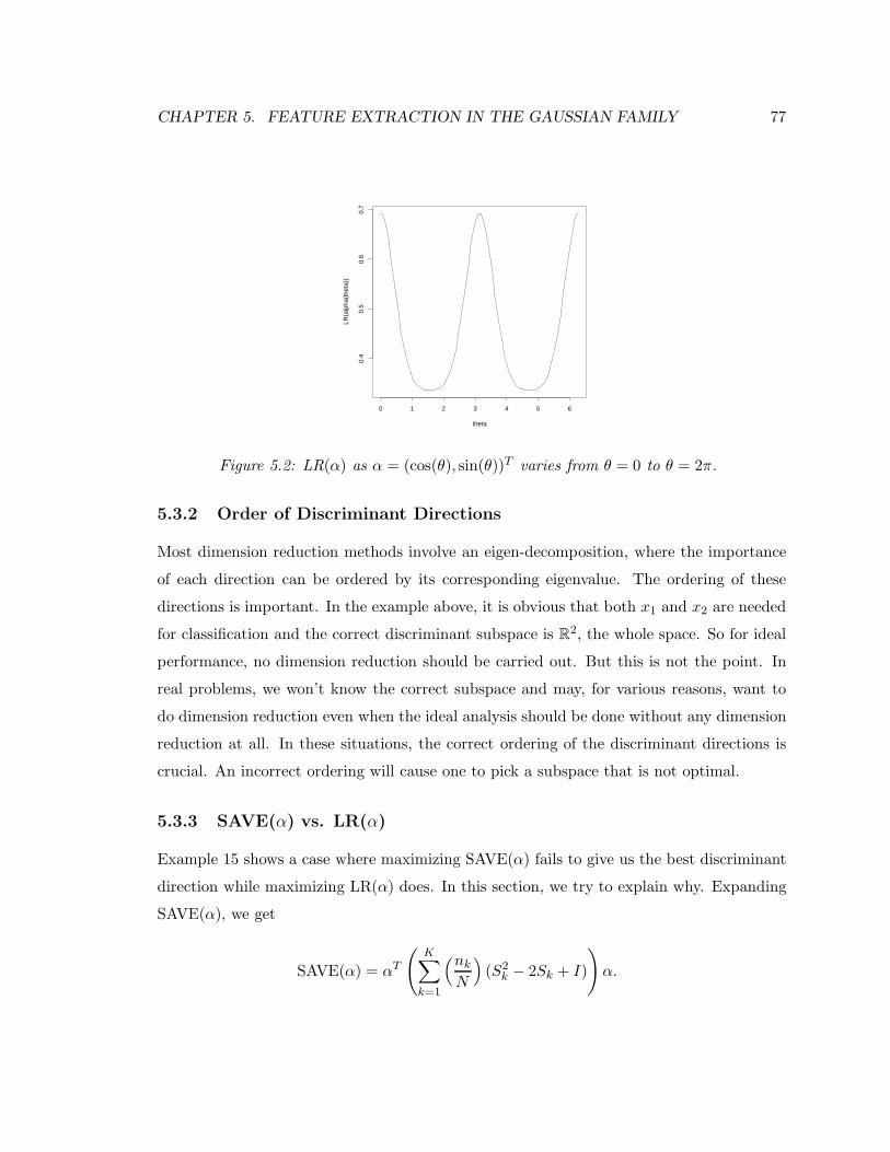
CHAPTER 5. FEATURE EXTRACTION IN THE GAUSSIAN FAMILY 77
theta
LR(a
lpha
(the
ta))
0 1 2 3 4 5 6
0.4
0.5
0.6
0.7
Figure 5.2: LR(α) as α = (cos(θ), sin(θ))T varies from θ = 0 to θ = 2π.
5.3.2 Order of Discriminant Directions
Most dimension reduction methods involve an eigen-decomposition, where the importance
of each direction can be ordered by its corresponding eigenvalue. The ordering of these
directions is important. In the example above, it is obvious that both x1 and x2 are needed
for classification and the correct discriminant subspace is R2, the whole space. So for ideal
performance, no dimension reduction should be carried out. But this is not the point. In
real problems, we won’t know the correct subspace and may, for various reasons, want to
do dimension reduction even when the ideal analysis should be done without any dimension
reduction at all. In these situations, the correct ordering of the discriminant directions is
crucial. An incorrect ordering will cause one to pick a subspace that is not optimal.
5.3.3 SAVE(α) vs. LR(α)
Example 15 shows a case where maximizing SAVE(α) fails to give us the best discriminant
direction while maximizing LR(α) does. In this section, we try to explain why. Expanding
SAVE(α), we get
SAVE(α) = αT
(
K∑
k=1
(nk
N
)
(S2k − 2Sk + I)
)
α.
CHAPTER 5. FEATURE EXTRACTION IN THE GAUSSIAN FAMILY 78
By a second-order Taylor expansion (log x ≈ −x2/2 + 2x − 3/2) on LR(α), we can get
(noting the constraint αT α = 1)
LR(α) ∝K∑
k=1
(nk
N
)
(
1
2(αT Skα)2 − 2(αT Skα) + (αT Iα)
)
+ const
= αT
(
K∑
k=1
(nk
N
)
(SkWαSk − 2Sk + I)
)
α + const,
where
Wα =1
2ααT .
Therefore, we can see that SAVE(α) is essentially a second-order approximation to LR(α),
but with an added simplification that Wα = I. We are not able to develop an intuition for
this simplification. In example 15, we saw that this simplification might have caused SAVE
to identify the incorrect discriminant direction.
Remark 5.5 In this chapter, LR(α) has been adapted specifically to QDA. Therefore,
one might wonder if the success of LR(α) over SAVE(α) in example 15 is specific to the
underlying classes being Gaussian. Here, we create a very similar situation, except this time
the data are generated from uniform (very non-Gaussian) densities. The data (left panel of
figure 5.3) are generated as follows:
Class 1 : x1 ∼ Uniform(0.5, 1), x2 ∼ Uniform(0, 1)
Class 2 : x1 ∼ Uniform(0, 0.6), x2 ∼ Uniform(1/3, 2/3)
We can easily verify in a similar fashion that x1, the direction of mean separation, is still
the better discriminant direction than x2, the direction of variance difference. The middle
and right panels of figure 5.3 show LR(α) and SAVE(α) (both computed using sample
covariances) as α goes around the unit circle from 0 to 2π. Again, we see that SAVE
continues to favor x2 (θ = π/2, 3π/2) while LR favors x1 (θ = 0, π, 2π).
Remark 5.6 We’ve emphasized the importance of being able to order the discriminant

CHAPTER 5. FEATURE EXTRACTION IN THE GAUSSIAN FAMILY 79
Data
x1
x2
0.0 0.2 0.4 0.6 0.8 1.0
0.0
0.2
0.4
0.6
0.8
1.0
11
1
1
1
1
1
1
1
1
1
1
1
1 1
11
1
1
1
1
1
1
1
1
1
1
1
1
1
11
1
11
1
1
1
1
1
1
1
1
1
1
1
1
1
1
1
1
1
1
11
1
1
1
1
1
1
11
1
1
11
1
1
1
1
111
1
1
1
11
1
1
1
1
1
1
1
1
11
1
1
1
1
1
1
1
1
1
1
1
2 22
2
2
2
2
2
2
2 2
22
2
2
22
2
22
2
22
2
2
2
22
2
2
2
22
2
22
2
2
2
22
2 2
2
2
2
2
2
2
2
2
2
2
22
22
2
2
2
2
2
2
2
22 2
22
2
2
2
2
2
2
2
22
22
2
22
2
2
2
2
2
2 2
2
222
2
2
22
22
LR
theta
0 1 2 3 4 5 6
0.6
0.8
1.0
1.2
SAVE
theta
0 1 2 3 4 5 6
1.05
1.10
1.15
1.20
1.25
Figure 5.3: LR vs. SAVE on uniform data.
directions correctly. Since LR is optimized numerically, it is possible for our procedure to
be trapped in a local maximum, thereby giving the wrong ordering as well. This problem
may seem to be even more serious in our general implementation where we incorporate
non-parametric methods for estimating the (marginal) densities. However, such problems
can usually be mitigated quite effectively by selecting large bandwidths when estimating the
densities. Figure 5.4 shows the LR function for the uniform example above as α goes around
the unit circle, estimated using our general implementation and with different bandwidths.
With a large bandwidth, the local maximum essentially disappears.
LR: Bandwidth=0.6
theta
0 1 2 3 4 5 6
4060
8010
012
0
LR: Bandwidth=0.9
theta
0 1 2 3 4 5 6
4060
8010
0
Figure 5.4: LR computed on simulated data as depicted in figure 5.3, using non-parametricdensity estimates with different bandwidths. A low bandwidth leads to a rough estimate witha local maximum while a large bandwidth smoothes away the local maximum.
CHAPTER 5. FEATURE EXTRACTION IN THE GAUSSIAN FAMILY 80
5.4 Feature Extraction with Common Principal Components
In the preceding sections of this chapter, we often used a simple case to help us gain
some intuition and insight, i.e., a special case where the Sk’s all have common eigenvectors
Sk = UΛkUT where
Λk = diag(λ1k, λ2k, ..., λdk).
This is called the common principal component (CPC) model and was extensively studied
by Flury (see [9]). In this section, we develop a variation for feature extraction in this
special case.
5.4.1 Uniform Dissimilarity
Example 15 actually satisfies the CPC model. There we noticed that LR(α) achieved
its maximum at one of the common eigenvectors. This did not just happen accidentally.
Result 5.1 below tells us that under the CPC model, it is often unnecessary to search over
the entire space for the optimal discriminant direction. Instead, we can usually restrict our
attention to a finite set of directions: namely, the common eigen-directions, u1, u2, ..., ud.
This provides a great deal of analytic convenience, which we exploit in section 5.4.3 to gain
some further insights. To prove this result, we need some definitions.
Definition 5.1 A vector w ∈ Rd is called a weighting if
d∑
j=1
wj = 1, and wj ≥ 0 ∀ j.
Definition 5.2 We define the average eigenvalue of Sk with respect to weighting w as
φk(w)=
d∑
j=1
wjλjk.

CHAPTER 5. FEATURE EXTRACTION IN THE GAUSSIAN FAMILY 81
Definition 5.3 Suppose the Sk’s have common eigenvectors, Sk = UΛkUT , then the eigen-
directions ui and uj are dissimilar with respect to weighting w if
∑
k
(nk
N
)
(
λik
φk(w)
)
6=∑
k
(nk
N
)
(
λjk
φk(w)
)
. (5.4.13)
They are uniformly dissimilar if they are dissimilar with respect to all weightings w ∈ Rd.
Result 5.1 Suppose the Sk’s have common eigenvectors, Sk = UΛkUT . If uj and ui are
uniformly dissimilar for all j 6= i, then LR(α) as in equation (5.3.10) is maximized by the
eigen-direction uj for which
K∑
k=1
(nk
N
)
(− log λjk) (5.4.14)
is the largest.
Proof Since the Sk’s have common eigen-directions, we can simply choose to work in the
basis of u1, u2, ..., ud. By writing out LR(α) explicitly, our problem becomes
maxK∑
k=1
(nk
N
)
− log
d∑
j=1
α2jλjk
subject tod∑
j=1
α2j = 1.
The Lagrangian function for this constrained optimization problem is
K∑
k=1
(nk
N
)
− log
d∑
j=1
α2jλjk
− θ
d∑
j=1
α2j − 1
and the first order conditions are
∑
k
2(nk
N
)
αjλjk∑
jα2
jλjk
− 2θαj = 0 ∀ j,
or
αj
[
∑
k
(nk
N
)
(
λjk
φk(α2)
)
− θ
]
= 0 ∀ j,
CHAPTER 5. FEATURE EXTRACTION IN THE GAUSSIAN FAMILY 82
where
φk(α2)
=∑
j
α2jλjk.
Therefore, for every j, either
αj = 0
or
∑
k
(nk
N
)
(
λjk
φk(α2)
)
= θ. (5.4.15)
Since the eigen-directions are uniformly dissimilar for every j 6= i, this means there exists
at the most one j = j∗ for which (5.4.15) can be true. The fact∑d
j=1 α2j = 1 means that
the optimal α must be 1 at the j∗-th position and 0 everywhere else. Plugging this back to
the objective function, we get
LR(α) ∝K∑
k=1
nk (− log λj∗,k) + const.
Obviously, the correct j∗ that maximizes this is
j∗ = argmaxj
K∑
k=1
nk (− log λjk) .
This ends the proof.
Remark 5.7 Here is how one should understand the notion of uniform dissimilarity. φk(w)
is a weighted average of the eigenvalues within class k, averaged across dimensions; hence
λjk/φk(w) can be regarded as a standardized eigenvalue. Then
∑
k
(nk
N
)
(
λjk
φk(w)
)

CHAPTER 5. FEATURE EXTRACTION IN THE GAUSSIAN FAMILY 83
can be regarded as a weighted average of the (standardized) eigenvalues in the j-th eigen-
direction, averaged across classes. Hence the notion of uniform dissimilarity means the
following: no matter how you standardize the eigenvalues within each class, when averaged
across classes the eigenvalues for all the eigen-directions are still different from one another.
This is intuitive. If any two eigen-directions are not “dissimilar” enough, it will be hard for
us to distinguish their discriminatory power.
Remark 5.8 In example 15, it is easy to verify that the two eigen-directions are uniformly
dissimilar: there is no w between 0 and 1 such that
0.5
0.5w + 0.3(1 − w)+
0.5
0.5w + 1.7(1 − w)=
0.3
0.5w + 0.3(1 − w)+
1.7
0.5w + 1.7(1 − w).
Our result then implies that we just have to compare the two eigen-directions according to
e1 =1
2(− log 0.5− log 0.5) ≈ 0.69,
e2 =1
2(− log 0.3− log 1.7) ≈ 0.34.
Since e1 > e2, we arrive at the same conclusion as before (section 5.3.1): i.e., x1 is the best
discriminant direction.
Remark 5.9 In the unlikely event that there is a particular weighting w for which all the
eigen-directions can be “similarized” in the sense that
∑
k
(nk
N
)
(
λik
φk(w)
)
=∑
k
(nk
N
)
(
λjk
φk(w)
)
∀ i 6= j,
then any α with α2m = wm for m = 1, 2, ..., d would be a stationary point. But since such
w “similarizes” all the directions, we conjecture that any corresponding α is more likely to
be a minimizer rather than a maximizer, if not a saddle point.
Remark 5.10 In the less extreme case that there is a particular weighting w for which
some (but not all) eigen-directions, say ui and uj , can be “similarized” in the sense that
∑
k
(nk
N
)
(
λik
φk(w)
)
=∑
k
(nk
N
)
(
λjk
φk(w)
)
,

CHAPTER 5. FEATURE EXTRACTION IN THE GAUSSIAN FAMILY 84
then any α with α2m = wm for m = 1, 2, ..., d could potentially be a stationary point. But
for it to actually be a stationary point, the first order condition still requires that at most
two of the αm’s be non-zero, namely αi and αj. We conjecture that the chance for such a
coincidence is very small.
5.4.2 Special Algorithm
Result 5.1 allows us to design another specialized feature extraction algorithm (see algo-
rithm 5.1). It is worth pointing out that this special algorithm is not suitable when the
Algorithm 5.1 Feature Extraction under Common Principal Components
1. Standardize the data: z = S−1/2x.
2. Fit a common principal component model for the K classes. This can be achievedby the FG algorithm, developed by Flury and Gautschi (see [9] for details and itsconvergence properties). Denote the common eigenvectors uj , j = 1, 2, ..., d.
3. For each Sk, compute λjk = (UT SkU)jj, j = 1, 2, ..., d, where Mjj denotes the (j, j)-thdiagonal element of the matrix M .
4. Return S−1/2uj as the features in the original space. The importance of these featuresfor discrimination is ranked according to equation (5.4.14).
CPC model does not hold, because the CPC-basis is not necessarily an optimal basis for
discrimination. The only criterion used for constructing the CPC-basis is simultaneous
diagonalizability (see [9]). Therefore CPC is a dictionary method and result 5.1 merely
provides a recipe (criterion) for ranking and selecting the correct variables within the CPC-
dictionary. As we illustrated in example 11, section 4.2, variable selection inside a dictionary
that is not optimally constructed for discrimination may not be as effective as direct feature
extraction. For example, in section 4.5 of [9], Flury concluded that the CPC model does not
fit the Fisher’s Iris data — a canonical dataset for feature extraction — “at any reasonable
level of significance.”
Since it is not necessary to search over the entire space, it might appear (falsely) that
algorithm 5.1 is a faster algorithm. Here, it is worth pointing out that the FG-algorithm

CHAPTER 5. FEATURE EXTRACTION IN THE GAUSSIAN FAMILY 85
needed to find the CPC-basis is not a fast algorithm. In this sense, the need to consider only
a finite number of directions is primarily an analytic convenience, rather than a practical
one.
On the other hand, numerical optimization using variations of Newton’s method has its
own problems, e.g., the problem of local solutions. In this sense, using the FG-algorithm
and evaluating the common principal directions by equation (5.4.14) can be a numerically
more stable alternative, especially when the data can be reasonably approximated by the
CPC model.
5.4.3 SAVE(α) vs. LR(α): An Experiment
In section 5.3.3, we offered one explanation of why LR works better than SAVE. We showed
that SAVE is a second-order approximation to LR with an extra mysterious simplification
that can’t easily be justified. Result 5.1 allows us to conduct a simple experiment on ex-
ample 15 to gain some further insight.
We first fix everything along x2 for both classes as they were before and, again, force
the two classes to have the same marginal variance along x1. Let µ1 = (−√
b, 0)T and
µ2 = (√
b, 0)T , where b is a now free parameter. Since result 5.1 is derived for standardized
data, the value b affects not only the mean separation between the two classes, but also
their marginal variances along x1: If b is large, the between-class variance is large, forcing
the within-class variance to be small, and vice versa. In particular, the marginal variance
along x1 must be 1 − b for both classes. Therefore b is only free to move within the unit
interval.
As b changes, the Bayes misclassification rate of y1 will change. We can imagine as b
moves from 1 to 0, x1 will at some point cease to be the best discriminant direction and x2
will take over. Therefore the first question we ask is: at what value of b does this reversal
take place? As b changes, the maxima for LR(α) and SAVE(α) will also change. Note that
there is no need to be concerned about directions other than x1 and x2, due to result 5.1,
so we simply ask: at what value of b will LR(α) and SAVE(α) start to pick x2 over x1 as
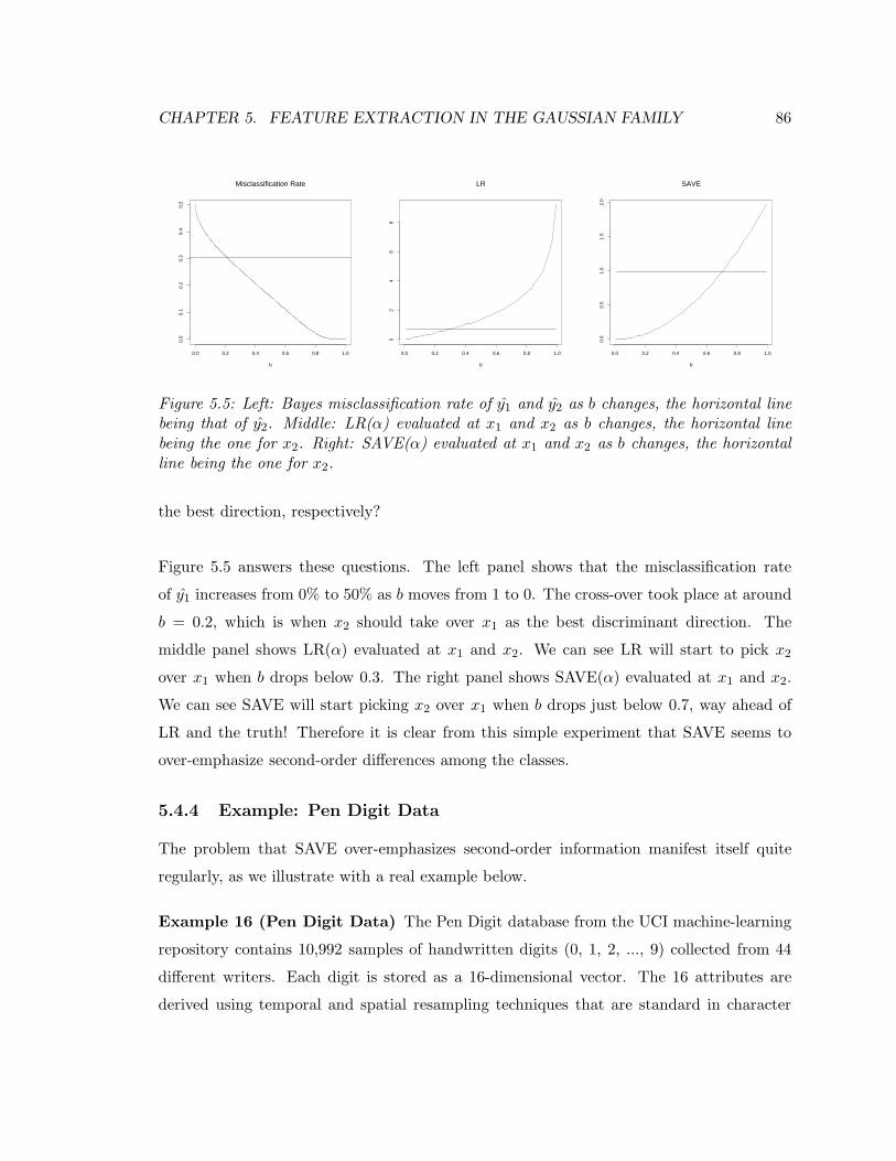
CHAPTER 5. FEATURE EXTRACTION IN THE GAUSSIAN FAMILY 86
Misclassification Rate
b
0.0 0.2 0.4 0.6 0.8 1.0
0.0
0.1
0.2
0.3
0.4
0.5
LR
b
0.0 0.2 0.4 0.6 0.8 1.0
02
46
8
SAVE
b
0.0 0.2 0.4 0.6 0.8 1.0
0.0
0.5
1.0
1.5
2.0
Figure 5.5: Left: Bayes misclassification rate of y1 and y2 as b changes, the horizontal linebeing that of y2. Middle: LR(α) evaluated at x1 and x2 as b changes, the horizontal linebeing the one for x2. Right: SAVE(α) evaluated at x1 and x2 as b changes, the horizontalline being the one for x2.
the best direction, respectively?
Figure 5.5 answers these questions. The left panel shows that the misclassification rate
of y1 increases from 0% to 50% as b moves from 1 to 0. The cross-over took place at around
b = 0.2, which is when x2 should take over x1 as the best discriminant direction. The
middle panel shows LR(α) evaluated at x1 and x2. We can see LR will start to pick x2
over x1 when b drops below 0.3. The right panel shows SAVE(α) evaluated at x1 and x2.
We can see SAVE will start picking x2 over x1 when b drops just below 0.7, way ahead of
LR and the truth! Therefore it is clear from this simple experiment that SAVE seems to
over-emphasize second-order differences among the classes.
5.4.4 Example: Pen Digit Data
The problem that SAVE over-emphasizes second-order information manifest itself quite
regularly, as we illustrate with a real example below.
Example 16 (Pen Digit Data) The Pen Digit database from the UCI machine-learning
repository contains 10,992 samples of handwritten digits (0, 1, 2, ..., 9) collected from 44
different writers. Each digit is stored as a 16-dimensional vector. The 16 attributes are
derived using temporal and spatial resampling techniques that are standard in character

CHAPTER 5. FEATURE EXTRACTION IN THE GAUSSIAN FAMILY 87
LDA
10 15 20
-14
-12
-10
-8-6
-4
99
9
9
9
0
0
9
0
6
6
6
0 0
9
0
9
6
0
9
6
0
0
6
9
9
0
9
0
0
0
9
0
0
9
9
0
6
9
6
6
0
0 0
0
0
0
6
9
0 0
9 9
6
6
0
9
6
0
6
0
6
0
0
6 6
9
0
6
9
0
9 0
6
6
66
0
99
6
6
0
6
6
9
0
9
0
0
6
9
0
0 0
6
0
6
9
6
6
9
0
66
9
0
99
9
6
0 0
9
6
6
0 0
9
6
6
66
09
9
0
9
9
0
6
0
0
9
0
6
9
6
0
0
6
9
0
6
6
9
0
6
6
6
9
6
6
9
6
9
0
9
6
0
9
0
0
9
6
0
9
0
0 0
99
6
0
6
0
0
6
9
0
6
0
99
09
0
0
9 9
0 0
9
666
0 0
99
0
6
6
0
9
0 0
6
6
0
9
6
0 0
666
0
0
09
9
0
9
9
0
6
9
0
6
6 9
0
6
9
6
6
6
0
6 6
6
0
0
6
6
6 6
99
6 6
9
0
9
9
6
0
6
0
9
9
9
0 0 0
6
66
0
9
9
9
0
9
09
0
0
0
6
0
0 0
6
9
9
0
6
9
6
9
9
0
6 6
0
6
9
0
6
9
6
6
0
99
0 0
0
6
6
0
66
99
0
0
0
0
0
0
99
6
09
9
66
0
9
0
9
66
9
9
9
9
6
9
0
6
6
0
6
0
9
6
6
9
0
6
6
9
0
6
9
0
6
0
6
0 0
0
9
6
0
6
9 9
6 9
0
0
6
0
6
0
66
6
9
0
0
0
9
0
6
0
9
6
9
99
0
0
0 0
9
9
6
6
0
9
9
0
6
0
6
9
9
0
6
0
9
0
0 0
6
0
0
0
9
9
0 0
99
0
9
6
9
9
6
0
9
6
0
0
0
6
9
9
9
0
0
6
9
6
6
999
9
6
9
0
9
6
6
9
6
6
9
0 0
0 0
9
6
6
66
0
0
6
9
66
0
0
6
66
9
6
0
6 9
9
0
9
6
6
69
0 0
9
0
9
6
0
9
66
9
0
0
9
0
6
6
9
0
9
0
9
0
6 9
66
0
6
6
6
0
9
0
0
6
0
0 0
6
0
9
0
0
9
6
6
9
6
6
9
6
9
0
9
6
0
0
0
6
0
6
9
0
6
6
6
0
0
0
99
6
0
0
9
0
9
0
6
6
0
66
0
6
9
6
0
6
9
9
9 9
6
9
0
9
0
0 0
9
0
9
9
6
6
9
0
0
6
66
6
0
9
6
9
66
9
6
0
99
6
0
9
6
9
0
6
09
0
6
0
6
9
0 0
0
9
9
6
9
0
9
6
0
6
9 0
9
0
6
9
6
6
0
9
6
6
9
0
0
0
6 6
0
9
0
9
99
0
9
0 0
6
6
9
6
6
6
0 0
9
9
6
9
9
0
9
0
0
69
9
9
6
0
9
6
9
9
9
99
9
0
6
0
0 0 0
0
66
0
0
6
9
0
6
9 9
0 0 0 0
6
6
0
6
9
0
0
9
0
6
9
6
9
0
6
6
9
0
0
9
0
0
666
0
9
0
6
66
0
6
6
9
6
0
6
66
9
66 9
0
9
9
0
6 6
0
6
6
6
6
6
9
0
0
99
6
0
9
9
0
0
6
9
0
9
99
6
9
0
9
9
9
9
0 0
9
9 9
9
6
0
6
6
9
0
6
0
0
0
6
6
0
0
0
6
0
6
0
9
0
6
0
6
0
6 6
6
0
6
0
9
0
0
6
6
0
99
9
6
0
9
6
9
0
9
6
9 9
99
6 6
9
0
0
99
0
0
0
9
6
99
9
0
6
9
0
9 9
9
9
9
6
9
6
9
0
99
6
9
66
0
09
9
0 0
6
6
6
9
9
0
6
9
9
0
6
99
6
9
0 0
9
0
6
9
9
6
6
6
0
6
0
0
6
9
0
99
6
0
9
0
0
6
99
6
0
9
9
9
66
9
0
99
9
6
0
0
0
0
0
9
0
6
0 0
0
9
6
0 0 0
6
9
0
66
6
9
6
0
6
6
0 0 0 0 0
66
9
9
9
9
6
9
6
6
9
6
9
6 6
9
99
9
6
9
0
6
6
9
6
99
69
6
0
9
0 0
9
6
0 0
SAVE
-2 0 2 4
-20
24
9
9
9
9
9
0 0
9 066
6 0 0
9
09
6 0
9
6 0
069
9
0
9
0
0
0
9
0 0
9
9
06
9
6
6 0 0 0
0
0
0
6
9
0 0
9
9
66
0
9
6 0 6 06 0
066
9 0 6
9
0
9
0
6
66
6 0
9
9
66
066
9
0
9
0
06
9
0 0 06 0
6
9
6
6
9
066
9
0
9
9
96
0 0
9
66 0
0
9
6
666
0
9
9
0
99
06 0
0
9 0
6
9
6
0 06
9
0
669
0
6
6
6
9
66
9
69
0
96
09
0 0
9
6 0
9
0
0 09
9
6
06
0
0
6
9
0
6
0
9
9
0
9 0 0
9
9
0
0
9
6
66 0 0
9
9
06
6
0
9
0 06 6
09
6
0
0
6
66
0 0
0
9
9
0
9
9
0
6
9
0
66
9
06
9
666 066 6 0
0 6666
9
9
66
9
0
9
9
6 06 0
9
9
9 0
0
06
66
09
9
9
0
9
0
9
0 0 0 6 0
0 0
6
9
9 0 6
9
69
9
0
66 0
69
0
6
9
6
6 0
9
9
0 0 0
6
6 066
9
9
0
0 0
0 0
0
9
9
6 0
99 6
6
0
9
0
9
66
9
9
99
6
9
06
6 06 0
9
669
0
66
9
0
6
9
06 0
6 0 0
0
9
6 06
9
96
9
0 0 6 06 0 666
9
0
0
0
9
0 6 0
9
6
9
99
0 0 0 0
9
966
0
9
9
06
0
6
9
9
0
6 0
9
0 0 0
6
0
0
0
9
9
0 0
9
9
0
9
6
9
9
6 0
9
6
0 0
06
9
99
0 06
9 6 69
99
9
6
9
0
9
66
9
66
9
0 0
0
0
9
666
6 0
0
6
9
6
6
0 0
666
9
6 0
6
9
9
0
9
66
6
9
0 0
9 0
9
6 0
9
66
9
0 09 0 6
6
9
0
9
0
9
06
9
6
6 0
666
09 0
06 0
0 06
0
9 0 0
9
6
6
9
6
6
9
6
9
0
9
6 0
0 0
6
06
9
06
66
0
0
0
9
9
6
0 0
9
0
9
066
0
66 06
9
6 0 6
9
9
9
9
6
9
0
9
0
0
0
9
0
9 9
66
9
0
06
6
66
0
9
6
9
66
9
6
0
9
9
6 0
9
69
06
0
9
06 0
69 0 0
0
9
9
6
9
0
9
6
06
9
0
9
06
9
6
6 0
9
66
9
0 0
066
0
9
0
9
99 0
9
0
06
6
9
6
66 0 0
9
9
6
9
9
0
9 0
06
9
9
9
6
0
9
6
9
9
99
9
9
06
0 0
0 0 06
6
0 0
6
9
06
9
9
0 0
0 06
6 0
6
9
0 0
9
06
9
6
9
066
9
0 0
9
0 0 6 6 6 0
9
0 666
0
6
6
9
6
06 6
6
9
66
9
0
9
9
0 66 0
666 6
6
9
0
09
9
6
0
9
9
0
069
0
9
9
9
6
9
0
9
9
9
9
0 09
9
9
9
6 0
669
0 6
0
0
06
6 0
0 0 6
0
6 0
9
0
6 06
0
66
6 0
6 09
0 0
6
6
0
9
9
9
6
09
6
9
0
9
6
9
9
9
9
6
69
0
0
99
0
0 0
9
6
9
9
9
06
9
0
9
9
9
9
9
6
9
6
9 0
99
6
9
6
6
0
0
9
9 0
06
6
6
99 06
9
9
06
9
9
6
9
0
0
9
0
6
9
9
666
0
6 0
06
9
0
9
9
6 0
9
0
0
6
9
9
6
0
9
9
9
66
9
0
9
9
96 0
0 0 0
0
9
06
0 0 0
9
6 0
0 06
9
0
666
9
6 0
6
6
0 0 0 0
06
6
9
9
9
9
6
9
669
6
9
6
6
9
9
9
9
6
9
0
66
9
6
9
9
69
6 0
9
0 0
96
0
0
LR
-4 -3 -2
-4-3
-2-1
99
9
9
9
0
0
9
0
6
6
6
0 0
9
0
9
6
0
9
6
0
0
6
9
9
0
9
0
0 0
9
0
0
9
9
0
6
9
6
6
0
0 0
0
0
0
6
9
0 0
99
6
6
0
9
6
0
6
0
6
0
0
66
9
0
6
9
0
9 0
6
6
6 6
0
99
6
6
0
6
6
9
0
9
0
0
6
9
0
0 0
6
0
6
9
6
6
9
0
66
9
0
9
9
9
6
0 0
9
6
6
0 0
9
6
6
6
6
09
9
0
9
9
0
6
0
0
9
0
6
9
6
0
0
6
9
0
6
6
9
0
6
6
6
9
6
6
9
6
9
0
9
6
0
9
0 0
9
6
0
9
0
0 0
99
6
0
6
0
0
6
9
0
6
0
9
9
0
9
0 0
99
0 0
9
66 6
0 0
9
9
0
6
6
0
9
0 0
6
6
0
9
6
0 0
66
6
0 0
09 9
0
9
9
0
6
9
0
6
69
0
6
9
66
6
0
66
6
0
0
6
6
66
9
9
66
9
0
99
6
0
6
0
9
9
9
0
0 0
6
66
0
9
9
9
0
9 0
9
0
0
0
6
0
0 0
6
9
9
0
6
9
6
9
9
0
66
0
6
9
0
6
9
6
6
0
9
9
0 0
0
6
6
0
66
9
9
0
0
0
0
0
0
9
9
6
09
9
66
0
9
0
9
66
9
9
9
9
6
9
0
6
6
0
6
0
9
6
6
9
0
6
6
9
0
6
9
0
6
0
6
0 0
0
9
6
0
6
99
69
0
0
6
0
6
0
66
6
9
0
0
0
9
0
6
0
9
6
9
9 9
0
0
0 0
9
9
6
6
0
9
9
0
6
0
6
9
9
0
6
0
9
0
0 0
6
0
0
0
9
9
0 0
99
0
9
6
9
9
6
0
9
6
0
0 0
6
9
99
0 0
6
9
66
99
9
9
6
9
0
9
66
9
66
9
0 0
0 0
9
6
6
66
0 0
6
9
66
0
0
6
66
9
6
0
69
9
0
9
6
6
69
0 0
9
0
9
6
0
9
66
9 0
0
9
0
6
6
9
0
9
0
9
0
6
9
66
0
6
6
6
0
9
0
0
6
0 0 0
6
0
9
0 0
9
6
6
9
6
6
9
6
9
0
9
6
0
0
06
0
6
9
0
6
6
6
0
0
0
99
6
0
0
9
0
9
0
6
6
0
66
0
6
9
6
0
6
9
9
99
6
9
0
9
0
0
0
9
0
9
9
6
6
9
0 0
6
66
6
0
9
6
9
66
9
6
0
99
6
0
9
6
9
0
6
0
9
0
6
0
6
9
0 0
0
9
9
6
9
0
9
6
0
6
9
0
9
0
6
9
6
6
0
9
6
6
9
0
0
0
6
6
0
9
0
9
99
0
9
0 0
6
6
9
66
6
0
0
9
9
6
9
9
0
9
0
0
69 9
9
6
0
9
6
99
9
9
9
9
0
6
0
0 0 0
0
6 6
0
0
6
9
0
6
99
0 0 0 0
6
6
0
6
9
0
0
9
0
6
9
6
9
0
6
6
9
0
0
9
0
0
66
6
0
9
0
6
6 6
0
6
6
9
6
0
6
66
9
66
9
0
9
9
0
66
0
6
6
6
6
6
9
0
09
9
6
0
9
9 0
0
6
9
0
9
99
6
9
0
9
9
9
9
0 0
9
99
9
6
0
6
6
9
0
6
0
0
0
6
6
0
0
0
6
0
6
0
9
0
6
0
6
0
66
6
0
6
0
9
0
0
6
6
0
99
9
6
0
9
6
9
0
9
6
99
9
9
66
9
0
0
99 0
0 0
9
6
99
9
0
6
9
0
9
9
99
9
6
9
6
9
0
99
6
9
6
6
0
0
9
9
0 0
6
66
9
9
0
6
9
9
0
6
99
6
9
0 0
9
0
6
9
9
6
6
6
0
6
0
0
6
9
0
99
6
0
9
0 0
6
9
9
6
0
9
9
9
6
6
9
0
9
9
9
6
0
0
0
0
0
9
0
6
0 0
0
9
6
0 0 0
6
9
0
66
6
9
6
0
6
6
0 0 0
0 0
6
6
9
99
9
6
9
6
6
9
6
9
66
9
99
9
6
9
0
6
6
9
6
99
69
6
0
9
0 0
9
6
0 0
Figure 5.6: Pen Digit Data. Shown here are test data projected onto the leading 2 discrim-inant directions found by LDA, SAVE and LR, respectively.
recognition. More details are available from the UCI FTP site1. For our purposes, it suffices
to state that this is a 10-class problem in a 16-dimensional space. The dataset is divided
into a learning set (7494 case) and a test set (3498 cases).
For better graphical display, we only select the 6’s, 9’s and the 0’s, three easily confus-
able digits, as an illustration. For this 3-class sub-problem, there are 2219 cases in the
training set and 1035 cases in the test set. We apply LDA, SAVE and LR to the 3-class
sub-problem. In each case, we search for the 2 leading discriminant directions. We then
project the test data onto these 2 directions. Figure 5.6 shows the results. This is a real
problem, so we don’t know the true discriminant subspace. However, from the graphs, it
is clear that LDA separates the classes reasonably well. SAVE, on the other hand, picks a
subspace in which the 9’s have a much larger variance than the 0’s and the 6’s, while LR
picks essentially the same subspace as LDA.
5.5 Conclusion
Our examples in section 4.8 demonstrate that LDA as a feature extraction method is often
insufficient, and our criterion, LR, is capable of picking up important (high-order) features
that LDA leaves over. Our experiment in section 5.4.3 and the Pen Digit example in sec-
tion 5.4.4 deliver another important message. Here we see the strength (and robustness)
1 ftp://ftp.ics.uci.edu/pub/machine-learning-databases/pendigits/

CHAPTER 5. FEATURE EXTRACTION IN THE GAUSSIAN FAMILY 88
of LR over SAVE. While it is flexible enough to pick up high-order differences among the
classes, LR captures the right amount of trade-off and does not over-emphasize high-order
information when first-order differences are dominant.
SAVE originated as a variant of a well-known dimension reduction technique called Sliced
Inverse Regression (SIR) (see [28]). Both SIR and SAVE were first proposed as dimension
reduction techniques for regression problems. In essence, SIR consists of two steps. First,
it discretizes the regression response, y, into y. Then it performs LDA on the discretized
response. The discretization step converts a regression problem into a classification prob-
lem, so that the inverse regression function, E(x|y), is analogous to the class centroid, µk,
in the classification context.
SAVE was proposed because SIR, like LDA, apparently only uses the first-order information:
E(x|y). While SAVE attempts to consider second-order information, var(x|y) (analogous
to Sk), an important point we’ve made in this chapter is that it seems to over-emphasize
second-order information. It is therefore natural for us to suggest using the LR criterion
on discretized responses as a general dimension reduction technique for regression. We will
not, however, go into details in this thesis.

Chapter 6
Reduced-Rank Non-Parametric
Discrimination
So far in this thesis, we have focused on the general problem of dimension reduction and
feature extraction. Professor Jerome Friedman once commented that while the dimension
reduction problem is intellectually interesting on its own, its practical significance remains
unclear because it is not obvious how one should proceed afterwards. The correct under-
standing of this comment, we believe, is that it will be more valuable to incorporate di-
mension reduction and feature extraction components into predictive probabilistic models
(and come up with useful reduced-rank models), rather than develop stand-alone dimension
reduction techniques that are purely exploratory. In this chapter, we investigate one such
reduced-rank model that arises naturally in the context of our investigation.
In section 4.7, we considered the exploratory projection pursuit method for finding sub-
sequent discriminant directions. In chapter 3, we saw that most of the recent development
in discriminant analysis took place within the Gaussian framework, i.e., the density for the
k-th class is Gaussian, pk(x) ∼ N(µk,Σk), with various assumptions on µk and Σk. Extend-
ing discriminant analysis to a more general setting, where the class densities are modeled
non-parametrically, has always been a very hard problem, because it is extremely difficult
to estimate a multi-dimensional density function non-parametrically.
89
CHAPTER 6. REDUCED-RANK NON-PARAMETRIC DISCRIMINATION 90
In this regard, the rich projection pursuit paradigm allows a relatively easy integration
of the general dimension reduction technique developed in the previous chapters into a
non-parametric density model, making non-parametric discriminant analysis a practical
possibility.
First, we give a fairly detailed review of projection pursuit density estimation. There
are two associated algorithms, previously believed to be equivalent. Our study shows that
in the actual implementation the two algorithms differ non-trivially and actually lead to
different models. This difference has never been discovered elsewhere.
We then proceed to adopt these projection pursuit density models for non-parametric dis-
criminant analysis. Here we shall see that the difference in the two projection pursuit
algorithms will have significant consequences.
6.1 Projection Pursuit Density Estimation
Using projection pursuit, one can estimate an arbitrary high-dimensional density function
with
p(x) = p0(x)M∏
m=1
fm(αTmx). (6.1.1)
This was first proposed in 1984 in [15]. We start with an initial guess p0(x), usually an
easy-to-estimate parametric model such as a multivariate Gaussian, and find a series of
ridge modifications to get closer to the actual density function itself. Alternatively, one can
express this model recursively. At the m-th iteration, let pm−1(x) be the latest estimate of
p(x); then the goal is to find α and fm(·) to update the estimate by
pm(x) = pm−1(x)fm(αT x).
It is shown in [15] that for every fixed α the optimal ridge modification, fm(αT x), which
makes the updated estimate, pm(x), the closest (in terms of cross-entropy) to the true

CHAPTER 6. REDUCED-RANK NON-PARAMETRIC DISCRIMINATION 91
density, p(x), is given by
f(αT x) =p(α)(αT x)
p(α)m−1(α
T x). (6.1.2)
This is quite intuitive: for a given direction α, we simply divide out the marginal of our
current estimate and replace it with the correct marginal of the true density. If we keep on
doing this in all projections, we eventually get the true density itself. In practice we only
update in a few directions to get the best approximation. This is achieved by choosing a
direction, α, that maximizes the cross-entropy between pm(x) and p(x) at every step.
The most attractive and ingenious aspect of this method is that it avoids the “curse of
dimensionality” by decomposing the difficult high-dimensional density estimation problem
into a series of univariate density estimation problems.
6.1.1 Forward Algorithm
By equations (6.1.1) and (6.1.2), it is clear that at each iteration, m, we need to estimate
two univariate densities, p(α)(αT x) and p(α)m−1(α
T x). In fact, for the purpose of finding the
best direction, α, we need to estimate at least their first derivatives as well. In section 4.4,
we briefly addressed the problem of derivative estimation. Here we will treat these two
problems as a single block and simply refer to it as density estimation; but keep in mind
that it involves derivative estimation as well.
For a fixed direction, α, p(α)(αT x) is easy to estimate: we simply project the data onto
α and get z = αT x, and then estimate a univariate density (and its derivatives) for z. The
difficulty lies in the estimation of p(α)m−1(α
T x), the marginal density of the current density
estimate (and the related derivatives). The solution proposed in [15] is to use Monte Carlo
sampling:
• Since we know the current density estimate, pm−1(x), we can use Monte Carlo method
to draw a sample from pm−1(x), u1, u2, ..., uN.

CHAPTER 6. REDUCED-RANK NON-PARAMETRIC DISCRIMINATION 92
• Given u1, u2, ..., uN ∼ pm−1(x), p(α)m−1(α
T x) is then estimated by standard tech-
niques using the projected data, αT ui; i = 1, 2, ...,N.
Here we omit the details of Monte Carlo sampling. It is a separate topic on its own and is
not crucial for our presentation. A clear outline is given in the appendix of [15]. The entire
algorithm is contained in algorithm 6.1. The need for Monte Carlo makes the computation
Algorithm 6.1 Forward Projection Pursuit Density Estimation
• Start with p0(x), say, N(µ,Σ).
• For m = 1 to M :
– Choose a direction, α, where the distance between pm−1(x) and p(x) (in termsof cross-entropy) is the largest.
– Draw a Monte Carlo sample from pm−1(x) and estimate p(α)m−1(α
T x).
– Estimate p(α)(αT x) directly from the data.
– Update the density estimate by
pm(x) = pm−1(x)p(α)(αT x)
p(α)m−1(α
T x).
EndFor
quite cumbersome. A computationally more feasible method appeared three years later in
[11].
6.1.2 Backward Algorithm and Its Difficulties
In 1985, Huber (see [25]) discussed an alternative approach. Instead of constructing p(x) in
a forward fashion (called “synthetic” in [25]) from an initial guess p0(x), the whole process
can be turned backwards (called “analytic” in [25]). That is, we start with p(x) and move it
toward a target density q(x) by a series of ridge modifications, where q(x) is a simple known
density, say, the standard Gaussian. Here we expand this idea into a concrete outline for

CHAPTER 6. REDUCED-RANK NON-PARAMETRIC DISCRIMINATION 93
Algorithm 6.2 Backward Projection Pursuit Density Estimation
• Start with p0(x) = p(x), the actual density we wish to estimate.
• For m = 1 to M :
– Determine a direction, α, for ridge modification. Usually, we choose a directionwhere the distance between pm−1(x) and q(x) is the largest. Again, the distancebetween two densities is measured by the cross-entropy.
– Modify pm−1(x) in the α direction toward q(x). After the modification, the newdensity becomes
pm(x) = pm−1(x)q(α)(αT x)
p(α)m−1(α
T x),
where q(α)(·) = g(·) is usually the univariate standard Gaussian density.
EndFor
an algorithm (see algorithm 6.2). The entire process leads to the following model:
pM(x) = p0(x)M∏
m=1
q(αm)(αTmx)
p(αm)m−1 (αT
mx),
where pM (x) is sufficiently close to the target density, q(x). When turned backwards, this
equation gives a model for estimating the original density p(x) = p0(x):
p0(x) = q(x)M∏
m=1
p(αm)m−1(αT
mx)
q(αm)(αTmx)
. (6.1.3)
At a theoretical level, there is no apparent difference between the forward approach and
this backward approach; in fact, the two approaches seem entirely equivalent.
But it is not difficult to see from the algorithm we outline above that a difficulty remains
similar to that in the forward algorithm. At the m-th iteration, we must estimate p(αm)m−1 (·),
the marginal density of pm−1(x). Actually, this is even harder to achieve in this case. Be-
cause we start with something we know in the forward algorithm, we can actually evaluate

CHAPTER 6. REDUCED-RANK NON-PARAMETRIC DISCRIMINATION 94
pm−1(x) at every iteration; this allows us to draw Monte Carlo samples from it. Whereas
in the backward algorithm, we start with the density we wish to estimate, so we don’t even
know how to evaluate pm−1(x). As a result, even the computationally expensive Monte
Carlo is infeasible.
6.1.3 A Practical Backward Algorithm
A practical backward algorithm appeared two years later in [11], which we have already
seen in section 4.7.1 where it was presented slightly differently.
The key idea is as follows: at every iteration the density function changes due to the ridge
modification, so we transform the data as we go along in order to conform to the evolving
density (algorithm 6.1.3). The transformation of the data within every iteration is the key
element that makes the backward algorithm work, because we can now estimate p(α)m−1(α
T x)
directly from the (transformed) data. In fact, we don’t even need to resort to Monte Carlo.
In this sense, this algorithm provides a significant improvement over the forward algorithm.
But as we shall show in the next section, a significant price has to be paid for this computa-
tional simplification. This algorithm actually changes the density model of equation (6.1.3).
This important difference has not been discovered elsewhere and leads us to conclude that,
at a practical level, the forward and backward algorithms are not equivalent.
6.1.4 Non-equivalence Between the Forward and Backward Algorithms
We now study the backward algorithm in more detail. First, we show that equation (6.1.4)
is true.
Lemma 6.1 Suppose (x,y) ∼ p(x, y), where p(x, y) is the density for (x,y), x is one-
dimensional and y is multi-dimensional. Let
x′ = Φ−1(Fx(x))= γ(x), (6.1.5)
where Φ(·) is the standard normal cdf, and Fx is the marginal cdf of x. Let p′(x′, y) be the

CHAPTER 6. REDUCED-RANK NON-PARAMETRIC DISCRIMINATION 95
Algorithm 6.3 Feasible Backward Projection Pursuit Density Estimation
• Start with p(x), the actual density we wish to estimate.
• Repeat:
1. Determine a direction, α, for ridge modification.
2. Construct a transformation x′ = h(x) so that the marginal density of x′ agreeswith the target density, q, in the α direction, while in all directions orthogonal toα, it agrees with the original density, p. If we pick q to be the standard Gaussian,we can see that h(x) is exactly the same as defined in section 4.7.1:
h(x) = A−1(t(Ax)),
where A and t(·) are defined by equations (4.7.5) and (4.7.7), and the transfor-mation h(x) is defined by equation (4.7.6). In the next section we show thath(x) has density:
pm(h(x)) = pm−1(x)q(α)(γ(αT x))
p(α)m−1(α
T x), (6.1.4)
where q(α)(·) = g(·) is simply the univariate standard Gaussian density (Result6.1).
3. Let
x←− h(x).
EndRepeat
• Stop when the density of x is close enough to the target density, q.
CHAPTER 6. REDUCED-RANK NON-PARAMETRIC DISCRIMINATION 96
density for (x′,y); then
p′(x′, y) = p(γ−1(x′), y)
(
g(x′)
px(γ−1(x′))
)
. (6.1.6)
Remark 6.1 While (6.1.6) is the standard way of representing the density for (x′,y), we
prefer to write it as
p′(γ(x), y) = p(x, y)
(
g(γ(x))
px(x)
)
, (6.1.7)
because (x,y) is the original variable, and a transformation is applied to obtain (x′,y) =
(γ(x),y) and (6.1.7) allows us to keep track of the original and the transformed data more
directly. This will become handy as we go a few steps deep into the recursive iteration,
where it is much easier to keep track of a series of γ’s rather than a series of γ−1’s.
Proof By conditioning, we have
p′(x′, y) = p′(y|x′)p′x′(x′).
Since we only applied a monotonic transformation to x and didn’t do anything to y, we
have
p′(y|x′) = p(y|x),
for x′ = γ(x). And by definition of x′
p′x′(x′) = g(x′),
where g(·) is the standard normal density. Hence,
p′(x′, y) = p(y|x)g(x′)
=
(
p(x, y)
px(x)
)
g(x′)
= p(γ−1(x′), y)
(
g(x′)
px(γ−1(x′))
)

CHAPTER 6. REDUCED-RANK NON-PARAMETRIC DISCRIMINATION 97
or
p′(γ(x), y) = p(x, y)
(
g(γ(x))
px(x)
)
.
because x′ = γ(x).
The validity of equation (6.1.4) follows directly from the following theorem.
Result 6.1 Suppose x ∼ p(x). Then the density for h(x), where h(x) is defined by equation
(4.7.6), is given by
p′(h(x)) = p(x)
(
g(γ(αT x))
p(α)(αT x)
)
, (6.1.8)
where p(α)(·) is the marginal density of x in the α direction.
Proof Recall from section 4.7.1 that h(x) is defined as
xh−−−→ h(x)
yA
x
A−1
zt−−−→ t(z)
where A is an orthogonal rotation matrix such that
z= Ax =
αTx
A∗x
and
t(zj) =
γ(zj) for j = 1,
zj for j > 1.
The following diagram summarizes our notation for the density functions of x, z, h(x) and

CHAPTER 6. REDUCED-RANK NON-PARAMETRIC DISCRIMINATION 98
t(z):
p(x)h−−−→ p′(h(x))
yA
x
A−1
pz(z)t−−−→ p′z(t(z))
It now follows from the lemma that in the z-space,
p′z(t(z)) = pz(z)
(
g(γ(z1))
pz1(z1)
)
, (6.1.9)
where pz1(·) is the marginal density of z1. But the fact that z = Ax implies
pz(z) =1
|A| p(A−1z) =1
|A| p(x),
p′z(t(z)) =1
|A| p′(A−1t(z)) =1
|A| p′(h(x)).
Hence, (6.1.9) now implies
p′(h(x)) = p(x)
(
g(γ(αT x))
p(α)(αT x)
)
,
since by the definition of A, we have z1 = αTx.
With this result, we can now work out the details for the backward projection pursuit algo-
rithm and see that it transforms the density in successive steps, according to the following:
p0(x) = p(x),
p1(h1(x)) = p0(x)
(
g(γ1(αT1 x))
p(α1)0 (αT
1 x)
)
,
p2(h2(h1(x))) = p1(h1(x))
(
g(γ2(αT2 h1(x)))
p(α2)1 (αT
2 h1(x))
)

CHAPTER 6. REDUCED-RANK NON-PARAMETRIC DISCRIMINATION 99
and so on, where hm(x) transforms x in the αm direction as in the previous section and
leaves all orthogonal (relative to αm) directions unchanged. For simplicity, write
ρ0(x) = x,
ρ1(x) = h1(x),
ρ2(x) = h2 · h1(x),
...
ρM (x) = hM · hM−1 · ... · h1(x),
and we have, at the end of M iterations,
pM(ρM (x)) = p0(x)
M∏
m=1
(
g(γm(αTmρm−1(x)))
p(αm)m−1 (αT
mρm−1(x))
)
, (6.1.10)
where, again, pM(·) is sufficiently close to q(·). Turning this backwards, we get a model for
the original density:
p(x) = q(ρM (x))M∏
m=1
(
p(αm)m−1 (αT
mρm−1(x))
g(γm(αTmρm−1(x)))
)
. (6.1.11)
Note that this model is not at all the same model as equation (6.1.3) and, hence, is not equiv-
alent to the model given by the forward algorithm. Why is this the case? Here is the reason:
In the forward algorithm, as well as in equation (6.1.3), no transformation is introduced
to the original data, which makes it hard for us to estimate p(α)m−1(α
T x). But in the back-
ward algorithm, we actually transform the data at every step. This eliminates the need
for Monte Carlo, because the transformation makes the data conform to the density pm(x)
rather than to the original density p0(x) = p(x), which we start with. This allows us to
estimate p(α)m−1(α
T x) directly from the (transformed) data. In fact, recall that if we didn’t
introduce these transformations, the backward algorithm would have been hopeless in prac-
tice because even Monte Carlo would have been infeasible (see section 6.1.2). However, in
order to wrap around the entire process to obtain an estimate of the original density (prior

CHAPTER 6. REDUCED-RANK NON-PARAMETRIC DISCRIMINATION 100
to any of the transformations induced within the algorithm), we must unfold the entire
sequence of transformations.
In other words, in the forward algorithm, we must pay a price in Monte Carlo. In the
backward algorithm, although we can avoid the Monte Carlo step, we must pay a price (not
so much a computational one) to keep track of the sequence of transformations. Either way,
nothing comes out entirely free.
Despite the computational saving, the resulting density model from the backward algo-
rithm is much more cumbersome, because it involves the entire sequence of transformations
— although theoretically one can still use this model for density estimation as long as one
keeps good track of all the transformations. Notice that all of these transformations involve
only an orthogonal rotation and a monotonic one-dimensional transform. In terms of com-
putational cost, this is indeed cheaper than Monte Carlo. However, the resulting model is
cumbersome. In fact, it is no longer a clean-cut projection pursuit density model.
6.1.5 Projection Pursuit and Independent Component Analysis
It is important to point out that algorithms 4.4 and 6.1.3 are, in fact, the same exploratory
projection pursuit algorithm proposed in [11] by Friedman. We’ve simply presented it with
a slightly different emphasis depending on the context of our discussion. In section 4.7.1,
where our focus was the feature extraction problem, we emphasized the selection step, i.e.,
finding the interesting direction. In section 6.1.3, where our focus was the density estima-
tion problem, we emphasized the transformation step, i.e., transforming the data so that
the data conform to a density which we know how to compute.
Although the consequence of this exploratory projection pursuit algorithm is a more cum-
bersome density model, the algorithm itself is a perfectly valid one, especially in the context
of exploratory data analysis, such as finding interesting (e.g., non-Gaussian) directions in
the data. Recall that in section 4.7, we adopted the algorithm for the special purpose of
finding discriminant directions.

CHAPTER 6. REDUCED-RANK NON-PARAMETRIC DISCRIMINATION 101
The usefulness of exploratory projection pursuit is being re-discovered elsewhere, too. For
example, a connection has just recently been discovered between exploratory projection
pursuit and independent component analysis (ICA) (see [14], Chapter 13). ICA has an
extensive literature on its own. The original motivation of ICA is the well-known cocktail
party problem, where signals from several independent speakers are mixed together before
entering into each audio channel. In order to make sense of the mixed speech, we must be
able to unscramble the mixed signals and separate out the underlying independent signals,
i.e., identify independent components. Let X be the mixed signals (a multi-dimensional
object because the mixed signals are picked up from several different channels), properly
sphered to have unit variance in all directions. ICA seeks linear transformations of X,
Y = XA, such that the components of Y = (Y1, Y2, ..., YM )T are as independent as possible.
Let
H(Y ) = −∫
p(y) log p(y)dy
be the entropy of Y , then for properly constrained A (e.g., AT A = I and det(A) = 1), it
is shown in [14] that the components of Y are near-independent when∑
H(Ym) is small.
Since for fixed variance, the Gaussian distribution has the largest entropy, this means we
want to make Ym as non-Gaussian as possible. That is, ICA tries to find directions in
the data which have the maximal deviation from normality, an objective suitable for the
original exploratory projection pursuit algorithm!
6.2 Regularized Non-Parametric Discrimination
The model in (6.1.1) is a non-parametric model for a high-dimensional density and provides
a very appealing model for non-parametric discriminant analysis. In particular, we model
the density for class k as
pk(x) = p0(x)M∏
m=1
fmk(αTmx), (6.2.12)
CHAPTER 6. REDUCED-RANK NON-PARAMETRIC DISCRIMINATION 102
where from section 6.1 we know the ridge modification, for fixed αm, is simply
fmk(αTmx) =
p(α)k (αT
mx)
p(α)m−1,k(α
Tmx)
.
That is, we start with a common initial guess for all the classes, and augment each density
with a series of ridge modifications to distinguish the classes. Notice we force the ridge
directions to be the same for all the classes. In fact, at every iteration, we choose αm to
be the direction in which some measure of class difference is maximized. In section 4.3, we
proposed one such measure, namely, LR(α). Hence, the selection of ridge directions is a
feature extraction problem, for which we can fully exploit the materials in chapter 4. There
are several immediate advantages to this approach:
• We have a flexible, non-parametric model for the density functions in each class,
which allows us to model flexible decision boundaries, while still avoiding the “curse
of dimensionality.”
• The complexity of the model can be easily regularized by selecting only a few directions
where there are significant differences across classes.
• Therefore, although this is a density-based classification method, we actually do not
waste any effort in directions which may contain interesting features in the density
function itself but do not contribute to class differentiation.
• Because the initial density is common for all the classes, the decision boundary between
class k and K simply depends on the ratio of the augmenting ridge functions. In
particular, the decision boundary is characterized by
M∏
m=1
fmk(αTmx)
fmK(αTmx)
=
M∏
m=1
gmk(αTmx) = 1
or
M∑
m=1
log(gmk(αTmx)) = 0.
CHAPTER 6. REDUCED-RANK NON-PARAMETRIC DISCRIMINATION 103
This implies that there is a generalized projection pursuit additive model (see [34]
and section 3.1.3) for the posterior log-odds:
logp(y = k|x)
p(y = K|x)= log
πk
πK+ log
pk(x)
pK(x)= βk +
M∑
m=1
log(gmk(αTmx)),
where βk= log(πk/πK). Therefore, just as LDA leads to logistic regression and Naive
Bayes leads to GAM (section 3.3), non-parametric discriminant analysis using projec-
tion pursuit density leads to projection pursuit logistic regression. These connections
make it clear that this particular non-parametric model for discriminant analysis is
one level up from Naive Bayes in terms of its generality. Of course, our model is not
fully general because the αm’s are constrained to be the same for all k, but apparently
for good reasons.
Remark 6.2 The close connection between projection pursuit density estimation and pro-
jection pursuit logistic regression is also exploited in [14] for performing ICA. In particular,
it is shown that one can find independent components by first sphering the data and then
fitting a (constrained) projection pursuit logistic regression model on a two-class problem,
where one class is just the data (the mixed signals) themselves and the other, a background
class generated from a standard Gaussian density.
6.2.1 Forward Algorithm
Based on model (6.2.12), we can easily adapt the forward projection pursuit algorithm to a
procedure for non-parametric discrimination (algorithm 6.4). The computation, of course,
is quite involved. At every step, we must estimate a different ridge function for each class.
By equation (6.1.2), we know that for each ridge function fmk(·), we must estimate two
marginal densities, one of which requires Monte Carlo sampling (see section 6.1.1).
Remark 6.3 This remark outlines the key elements for maximizing LR(α) when pk(x) is

CHAPTER 6. REDUCED-RANK NON-PARAMETRIC DISCRIMINATION 104
Algorithm 6.4 Forward Projection Pursuit Discriminant Analysis
• Start with p0,k(x) = p0(x) ∀ k = 1, 2, ...,K, where p0(x) ∼ N(µ,Σ), and µ and Σ canbe estimated with maximum likelihood using the entire training set.
• For m = 1 to M :
– For fixed α, augment the density model for every class according to
pm,k(x) = pm−1,k(x)fmk(αT x).
and define
LR(α) = log
∏Kk=1
∏
xj∈Ckpm,k(xj)
∏Kk=1
∏
xj∈Ckpm(xj)
= log
∏Kk=1
∏
xj∈Ckpm−1,k(xj)fmk(α
T xj)∏K
k=1
∏
xj∈Ckpm−1(xj)fm(αT xj)
.
– Find αm = argmax LR(α). (See remark 6.3.)
– Update the density for each class:
pm,k(x) = pm−1,k(x)fmk(αTmx)
EndFor
CHAPTER 6. REDUCED-RANK NON-PARAMETRIC DISCRIMINATION 105
modeled non-parametrically using the special projection-pursuit density function in equa-
tion (6.2.12). At the m-th iteration, the objective function is
LR(α) = log
∏Kk=1
∏
xj∈Ckpm−1,k(xj)fmk(α
Tmxj)
∏Kk=1
∏
xj∈Ckpm−1(xj)fm(αT
mxj).
Hence at the m-th iteration, we simply solve the following optimization problem (suppress-
ing the index m on f , fk and α):
maxα
K∑
k=1
∑
xj∈Ck
(
log pm−1,k(xj) + log fk(αT xj)
)
−∑
xj
(
log pm−1(xj) + log f(αT xj))
.
Again, we can apply the standard Newton’s method to solve this optimization problem
numerically. Both the gradient and the Hessian can be written out explicitly:
g(r) =∂LR
∂αr=
K∑
k=1
∑
xj∈Ck
xrj
(
f′
k(αT xj)
fk(αT xj)− f
′
(αT xj)
f(αT xj)
)
and
H(r, s) =∂2LR
∂αr∂αs,
which, by writing zj = αT xj, is equal to
K∑
k=1
∑
xj∈Ck
xrj
(
f′′
k (zj)fk(zj)− (f′
k(zj))2
(fk(zj))2− f
′′
(zj)f(zj)− (f′
(zj))2
(f(zj))2
)
xsj.
These equations are exactly the same as equations (4.4.3) and (4.4.4), except the fk’s
and f mean slightly different things in the different contexts. To estimate g and H, all
we need to know is how to estimate the augmenting ridge functions and their first two
derivatives. Again, we do this once conditionally on each class to obtain fk, f′
k, f′′
k , and
once unconditionally over the entire training sample to obtain f, f′
, f′′
. Given α, write
z = αT x. Recall the ridge function is given by
f(z) =p(α)(z)
p(α)m−1(z)
.
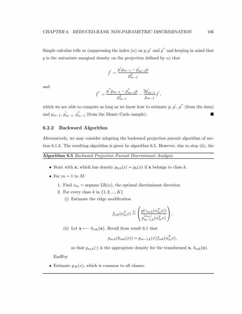
CHAPTER 6. REDUCED-RANK NON-PARAMETRIC DISCRIMINATION 106
Simple calculus tells us (suppressing the index (α) on p, p′
and p′′
and keeping in mind that
p is the univariate marginal density on the projection defined by α) that
f′
=p′
pm−1 − p′
m−1p
p2m−1
and
f′′
=p′′
pm−1 − p′′
m−1p
p2m−1
− 2p′
m−1
pm−1f
′
,
which we are able to compute as long as we know how to estimate p, p′
, p′′
(from the data)
and pm−1, p′
m−1, p′′
m−1 (from the Monte Carlo sample).
6.2.2 Backward Algorithm
Alternatively, we may consider adapting the backward projection pursuit algorithm of sec-
tion 6.1.3. The resulting algorithm is given by algorithm 6.5. However, due to step (ii), the
Algorithm 6.5 Backward Projection Pursuit Discriminant Analysis
• Start with x, which has density p0,k(x) = pk(x) if x belongs to class k.
• For m = 1 to M :
1. Find αm = argmax LR(α), the optimal discriminant direction.
2. For every class k in 1, 2, ...,K(i) Estimate the ridge modification
fmk(αTmx)
=
g(γm,k(αTmx))
p(αm)m−1,k(α
Tmx)
.
(ii) Let x←− hmk(x). Recall from result 6.1 that
pm,k(hmk(x)) = pm−1,k(x)fmk(αTmx),
so that pm,k(·) is the appropriate density for the transformed x, hmk(x).
EndFor
• Estimate pM (x), which is common to all classes.

CHAPTER 6. REDUCED-RANK NON-PARAMETRIC DISCRIMINATION 107
final x is not the same as the x we started with. In terms of the original data and according
to equation (6.1.11), the final density model for class k is
pk(x) = pM (ρM,k(x))
M∏
m=1
f−1mk(α
Tmρm−1,k(x)). (6.2.13)
For definition of ρm,k, see section 6.1.4. Several important issues must be pointed out:
• Although pM(·) is the same for all classes, the ρM,k(x) inside it is not. Therefore, we
still need pM (·) for classification purposes. Thus, unlike the forward algorithm, the
decision boundary between any two classes will no longer just depend on the ratio of
a series of ridge functions.
• In fact, because the data are transformed differently at each iteration for each class,
the ratio of two resulting “ridge functions” (for classes i and j) is
fm,i(αTmρm−1,i(x))
fm,j(αTmρm−1,j(x))
and is no longer a simple ridge function due to the function ρm−1,k(·) inside fmk(·).This means the posterior log-odds no longer simplifies to a generalized projection
pursuit additive model.
• That we need pM for classification is a serious problem, since pM is still a full multi-
dimensional density function which we must estimate. This is because we don’t usually
expect pM to be close enough to the known target density q. Since the goal is dis-
crimination rather than density estimation itself, it will often be the case that we’ve
only changed the original density in a few (M) discriminant directions. Therefore
although there may be very little difference across classes in pM after the proper
transformations, it is likely that pM is still quite different from q.
Therefore we can see that the difference between the forward and backward projection
pursuit algorithms is very significant.
CHAPTER 6. REDUCED-RANK NON-PARAMETRIC DISCRIMINATION 108
6.3 Illustration: Exclusive Or
We now illustrate the reduced-rank non-parametric discrimination procedure on a difficult
classification problem. There are four basic logical operators: “and,” “or,” “not” and “ex-
clusive or” (xor). All but “exclusive or” can be represented using a single-layer perceptron
model. Let x1 and x2 be two boolean variables taking values in −1, 1, corresponding to
F, T; and let I(A) be an indicator function such that
I(A) =
1 if A is true (T),
−1 if A is false (F).
Then the basic perceptron model has the form
I(w1x1 + w2x2 ≥ c)
for some weights w1, w2 and threshold c. Here is how the operators “and,” “or” and “not”
can each be represented by a perceptron model:
I (0.5x1 + 0.5x2 ≥ 1) ⇐⇒ x1 and x2,
I (0.5x1 + 0.5x2 ≥ 0) ⇐⇒ x1 or x2,
I(−x1 ≥ 0) ⇐⇒ not x1.
In order to represent the “exclusive or” operator, however, one must use a double-layer
perceptron model:
u = I (0.5x1 − 0.5x2 ≥ 1) =⇒ u = x1 and not x2,
v = I (0.5x2 − 0.5x1 ≥ 1) =⇒ v = not x1 and x2,
and
I (0.5u + 0.5v ≥ 0) ⇐⇒ u or v ⇐⇒ x1 xor x2.

CHAPTER 6. REDUCED-RANK NON-PARAMETRIC DISCRIMINATION 109
1/2 1/2
1/2
X1 X2
0
1/2
Xor
NotSingle-Layer Perceptron
OrAnd
1/2
X1 X2
-1/2-1/2
1 1
0
1/2
w1
c 0
X1
w2
X1 X2
-1
1/2
1
1/2
X1 X2
Figure 6.1: Graphical representation of perceptron models for the basic logical operators.X1,X2 are boolean variables taking values in −1, 1. A perceptron outputs 1 if w1x1 +w2x2 ≥ c and −1 otherwise. A negative weight indicates negation.

CHAPTER 6. REDUCED-RANK NON-PARAMETRIC DISCRIMINATION 110
A graphic representation of these models can be found in figure 6.1. Because of its complex-
ity, a pattern of the “exclusive or” nature is a difficult one to learn. We now demonstrate
that using flexible non-parametric density functions, one can readily overcome this difficulty.
Example 17 (Exclusive Or) To construct an “exclusive or” situation for classification,
let
µ1A =
1.5
1.5
, µ2A =
−1.5
−1.5
, µ1B =
−1.5
1.5
, µ2B =
1.5
−1.5
,
and consider two mixture classes, A and B, with
pA(x) =1
2φ(x;µ1
A, I) +1
2φ(x;µ2
A, I)
pB(x) =1
2φ(x;µ1
B , I) +1
2φ(x;µ2
B , I),
where φ(x;µ, I) denotes the N(µ, I) density function. Figure 6.2 shows one simulated in-
Data
x1
x2
-4 -2 0 2 4
-4-2
02
4
AA
A
AA
A
A
AA
A
A AA
A
A
A
AA
A
A
AA
A
A
A
A
A
A
A
A
AA
A
AA
AA
A
A
A
A A
AA
A
A
A
A
A
A
A
A
A
A
AA
A
AA
A
A
AA
A
A
AA A
A
A
A
A
A
A
A
A
A
A
A
A
A
A
AA
A
A
A
A
A
A
A
A
A
A
A
A
AA
A
A
A
A
AA A
A
AA
A
A
A
A
A
A
A
A
AA
A
A
AA
A
A
A
A
AAA A
A
A
A
A
AA A
AA
A
A
A
A
AA
A
A
AA
A
AA
A
AA
A
A
A
AA
A
A
A
A
A
A
A A
A
A
A
AAA
A
A
A
A
A
A
AA
A
A
A
A
A
A
A
A
A
A
A
A
A
A
AAA
A
A
AA
A
A
A
AA
A
A
A
A
A
A
A
AA
A
A
A
A
AA
AA
AA A
A
A
A
A
A
AA
A
A
A
A
A
AA
A
A
A
A AAAA
B
BB
B
BBB
BB
B
B
B
B
B
BB
BB
B
B
B
BB
B B
B
B
B
B
B
BB
BB
B
B
B
B
B
BB
BB
B
B
B
B
B
BB
B
BB
B
B
B
B
B
B
B B
B
B
B
B
B
B B
B
B
B
B
BBB
B
B
BB
B
B
B
B
B
B
B
BB
B
B BB
BB
B
BB
B
B
BB
BB
B
B
B
B
B
B
BB
B
BB B
B
BBB
B
B
B
B
B
B
B
B
B B
B
BB
B
BB
B
B B
B
B
B
B
B
B
BB
BB
BB
BBB
BB
B
BB B
B
BB
BB
B
B
B
B
B
B
BB
B
B
B
BB
BB
BB
B B
BB
B
B
B
B
BB
B
B
B B
B
B
B
B
B
B
B
BB
B
B
B
B
B
B
B BB
B
B B B
B
B
BB
B BBB
B
BB
B
B
B
B
B
B
B
B
BB
BB
B
B
B
B
B
BB
B
B
B
Figure 6.2: A simulated instance of the “exclusive or” situation in classification, nA =nB = 250.
stance of this situation. This is a particularly difficult problem, because when considered
alone, neither x1 nor x2 contains any information for classification; they must be considered

CHAPTER 6. REDUCED-RANK NON-PARAMETRIC DISCRIMINATION 111
together. The Bayes decision rule for this case is an “exclusive or” condition:
y =
B if (not (x1 > 0) and (x2 > 0)) or (not (x2 > 0) and (x1 > 0)),
A otherwise.
The symmetry makes it easy to compute the Bayes error for this problem:
2Φ(1.5)(1 − Φ(1.5)) ≈ 12.5%,
where Φ(x) is the standard normal cdf. We apply algorithm 6.4 to the data displayed in
-4
-2
0
2
4
x1
-4
-2
0
2
4
x2
00.
005
0.01
0.01
50.
02D
ensi
ty
Density For Class A
-4
-2
0
2
4
x1
-4
-2
0
2
4
x2
00.
005
0.01
0.01
50.
02D
ensi
ty
Density For Class B
Figure 6.3: Estimated density functions for the “exclusive or” data depicted in figure 6.2,after 2 ridge modifications.
figure 6.2. That is, we start with pA = pB = p0, where p0 is Gaussian, and modify each
by a series of ridge functions. The ridge directions are chosen to be directions in which
there are significant differences between the two classes (A and B). Figure 6.3 shows the
resulting density surfaces after 2 ridge modifications. The algorithm also produces a simple
classification rule, based on comparing the product of the ridge functions for each class.
The misclassification results on test data are summarized in table 6.1. We can see that
when we use 2 ridge modifications for each density function (the optimal number for this
problem), we can achieve an error rate very close to the Bayes error, despite the difficulty

CHAPTER 6. REDUCED-RANK NON-PARAMETRIC DISCRIMINATION 112
Number of Ridge Functions (M) Test Error
1 23.5%2 12.9%3 14.2%4 14.9%
Table 6.1: Misclassification error of algorithm 6.4 on 15,000 new observations. The Bayeserror for this problem is 12.5%.
of the problem!
Remark 6.4 We later discovered in [32] a similar attempt to use projection pursuit density
estimation for non-parametric discriminant analysis. However, there are some differences.
To choose the best ridge modification, we rely on the materials in chapter 4 and use the
log-likelihood-ratio criterion, LR(α), as our measure of class separation. In [32], the author
suggests minimizing the expected misclassification error directly. The author does realize,
however, that the apparent estimate of the expected misclassification error is discontinuous
in α, and proposes a (rather ad-hoc) smooth approximation. Our criterion is more direct and
systematic, particularly since Fisher’s LDA can be regarded as a special case (see section
4.3). We also investigated the backward projection pursuit algorithm and pointed out some
non-trivial differences and difficulties.

Chapter 7
Mixture Models
In chapters 4, 5 and 6, we’ve focused much of our attention trying to answer the following
question: how can we effectively do discriminant analysis when we allow the density func-
tions in each class to be non-parametric? In chapter 4, we focused on the general feature
extraction problem, aiming to overcome the curse of dimensionality. In chapter 5, we fo-
cused on a special case and compared our methods with a competitor, SAVE. In chapter
6, we investigated the possibility of using a special projection-pursuit density model for
(reduced-rank) non-parametric discriminant analysis.
Related to the idea of non-parametric discriminant analysis is an alternative approach,
which uses a mixture of Gaussians to model the density for each class (see e.g., [20]). Gaus-
sian mixtures can be viewed as an approximation to the non-parametric density. Hence it
is an intermediate approach, retaining the basic parametric structure and offering a certain
level of modeling flexibility at the same time. An advantage of the mixture approach is that
each mixture component can be viewed as a prototype.
In this chapter, we review an extension of the mixture approach, first outlined in [22].
Most of the materials in this chapter are not original for this thesis and should be viewed
largely as a review. But because of the connections with our main topics, we still treat this
material in some detail. What’s more, we shall see that this extension also turns out to
correspond to a natural generalization of the aspect model, which we introduced in chapter
113

CHAPTER 7. MIXTURE MODELS 114
1 — equation (1.3.1), to be specific.
7.1 Mixture Discriminant Analysis (MDA)
In [20], the class densities are modeled by a mixture of Gaussians, where every mixture
Gaussian component has the same covariance matrix:
pk(x) =
Rk∑
r=1
πkrφ(x;µkr,Σ). (7.1.1)
The covariance matrix, of course, need not be the same for every component, but it is
chosen to be the same in MDA for several reasons:
• Since the mixing parameters, πkr, are different for each class, the classes are not
restricted to have the same covariance matrix. In this sense, it is not necessary to use
different covariance matrices for each mixture component.
• In section 3.2.2, we already saw that estimating a separate covariance matrix for each
class could lead to unstable estimates and decision boundaries, and some regulariza-
tion was necessary. If each mixture component has a different covariance matrix, we
will be estimating several different covariance matrices within a single class. It is not
hard to imagine that this could easily lead to over-fitting.
• By using the same covariance matrix for all the components, MDA can be shown to be
equivalent to a weighted version of LDA (on the sub-classes). Therefore, the important
dimension reduction aspect of LDA carries over. Recall that prior to this thesis when
MDA was developed, there were no satisfactory dimension reduction techniques for
the case where pk ∼ N(µk,Σk). Hence in order to obtain low-dimensional views of the
data, it is necessary to constrain the covariances to be identical across all sub-classes.
Of course, this thesis significantly reduces such a concern.
We already know that for a two-class problem (K = 2), LDA can find only one (K − 1)
meaningful discriminant direction. By using a mixture for each class and creating multiple
sub-classes, it is possible to find multiple discriminant directions even for a two-class prob-
lem. This is one important improvement of MDA. The other important improvement, of

CHAPTER 7. MIXTURE MODELS 115
course, is that the decision boundaries are no longer constrained to be linear or quadratic.
7.2 LDA as a Prototype Method
A prototype method for classification works as follows: For each class, one or several pro-
totypes are chosen as representatives. To classify a new observation, its distances (in some
proper metric) to all the prototypes are calculated and compared, and it is assigned to the
same class as the prototype to which its distance is the shortest. The two crucial ingre-
dients, therefore, are the choice of the prototype(s) and the choice of the distance metric.
The K-nearest neighbor method (section 3.4) is a typical prototype method.
LDA can be viewed as a prototype method. Each class is modeled as a Gaussian, and
its centroid µk can be viewed as a prototype for class k. The distance metric is simply the
Mahalanobis distance. A new observation x is classified to the same class as the prototype
to which its Mahalanobis distance is the shortest, i.e.,
y = argmink
dM (x, µk)
= argmink
(x− µk)T Σ−1(x− µk).
Similarly, MDA can also be viewed as a prototype method, where each class is now repre-
sented by several prototypes, µkr, r = 1, 2, ..., Rk .
7.3 K-means vs. Learning Vector Quantization (LVQ)
The success of a prototype method depends critically on the choice of the prototypes. Below
we briefly review two well-known prototyping algorithms.
7.3.1 Separate K-means
On its own, K-means is a clustering algorithm. Given a set of points, it finds K prototypes
(cluster centers) that best represent the entire dataset. When applied to a classification
problem, K-means simply selects K prototypes separately for each class. The prototype

CHAPTER 7. MIXTURE MODELS 116
Algorithm 7.1 Separate K-means for Classification
• Prototype selection: Within each class k, apply K-means clustering and get a total ofJ prototypes mjk : j = 1, 2, ..., J ; k = 1, 2, ...,K.
• Classification: For any observation x, find its closest prototype and classify to the
associated class: class(x) = class
(
argminmjk
‖x−mjk‖)
.
selection for one class is independent of another. A point is classified to the same class as
its closest prototype. See algorithm 7.1.
Remark 7.1 For simplicity of presentation, we use the same number of prototypes for each
class but, in general, this certainly need not be the case.
Remark 7.2 Throughout this thesis, we have been using k = 1, 2, ...,K to index the classes,
so we use j = 1, 2, ..., J to index the prototypes within each class. In this sense, this
procedure is more appropriately called “separate J-means,” but we still call it “separate
K-means” since this is what the algorithm is generally known as.
7.3.2 Learning Vector Quantization (LVQ)
It is easy to see that the separate K-means algorithm does not use information efficiently,
because the prototypes are selected separately within each class, without regard to the
other classes. One can take other classes into account in order to place the prototypes more
strategically for classification. More specifically, one can move the prototypes for each class
away from the decision boundary. This is achieved by an algorithm known as learning vector
quantization (algorithm 7.2). The ǫ in algorithm 7.2 is a learning rate parameter. Figure
7.1 (taken from Professors Trevor Hastie and Robert Tibshirani’s course notes) shows how
LVQ improves on separate K-means. The prototypes are pushed away from the decision
boundary. As a result, the decision boundaries become smoother.
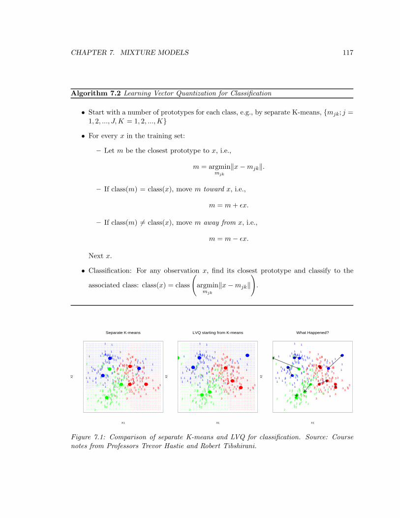
CHAPTER 7. MIXTURE MODELS 117
Algorithm 7.2 Learning Vector Quantization for Classification
• Start with a number of prototypes for each class, e.g., by separate K-means, mjk; j =1, 2, ..., J,K = 1, 2, ...,K
• For every x in the training set:
– Let m be the closest prototype to x, i.e.,
m = argminmjk
‖x−mjk‖.
– If class(m) = class(x), move m toward x, i.e.,
m = m + ǫx.
– If class(m) 6= class(x), move m away from x, i.e.,
m = m− ǫx.
Next x.
• Classification: For any observation x, find its closest prototype and classify to the
associated class: class(x) = class
(
argminmjk
‖x−mjk‖)
.
X1
X2
. . . . . . . . . . . . . . . . . . . . . . . . . . . . . . .. . . . . . . . . . . . . . . . . . . . . . . . . . . . . . .. . . . . . . . . . . . . . . . . . . . . . . . . . . . . .. . . . . . . . . . . . . . . . . . . . . . . . . . . . .. . . . . . . . . . . . . . . . . . . . . . . . . . . . .. . . . . . . . . . . . . . . . . . . . . . . . . . . .. . . . . . . . . . . . . . . . . . . . . . . . . . .. . . . . . . . . . . . . . . . . . . . . . . . . . .. . . . . . . . . . . . . . . . . . . . . . . . . . .. . . . . . . . . . . . . . . . . . . . . . . . . . .. . . . . . . . . . . . . . . . . . . . . . . . . . .. . . . . . . . . . . . . . . . . . . . . . . . . . .. . . . . . . . . . . . . . . . . . . . . . . . . . .. . . . . . . . . . . . . . . . . . . . . . . . . . .. . . . . . . . . . . . . . . . . . . . . . . . . . .. . . . . . . . . . . . . . . . . . . . . . . . . . .. . . . . . . . . . . . . . . . . . . . . . .. . . . . . . . . . . . . . . .. . . . . . . . . . . .. . . . . . . . . . .. . . . . . . . . . .. . . . . . . . . .. . . . . . . . . .. . . . . . . . .. . . . . . . . .. . . . . . . . . .. . . . . . . . . .. . . . . . . .. . . . . . . . .. . . . . . . . . . .. . . . . . . . . . . .. . . . . . . . . . . . .. . . . . . . . . . . . . .. . . . . . . . . . . . . .. . . . . . . . . . . . . . .
. . . . . . . . . . . . . . . . . . .. . . . . . . . . . . . . . . . . . .. . . . . . . . . . . . . . . . . . . .. . . . . . . . . . . . . . . . . . . . .. . . . . . . . . . . . . . . . . . . . .. . . . . . . . . . . . . . . . . . . . . .. . . . . . . . . . . . . . . . . . . . . . .. . . . . . . . . . . . . . . . . . . . . . .. . . . . . . . . . . . . . . . . . . . . . .. . . . . . . . . . . . . . . . . . . . . . .. . . . . . . . . . . . . . . . . . . . . . .. . . . . . . . . . . . . . . . . . . . . . .. . . . . . . . . . . . . . . . . . . . . . .. . . . . . . . . . . . . . . . . . . . . . .. . . . . . . . . . . . . . . . . . . . . . .. . . . . . . . . . . . . . . . . . . . . . .. . . . . . . . . . . . . . . . . . . . . . .. . . . . . . . . . . . . . . . . . . . . . .. . . . . . . . . . . . . . . . . . . . . . .. . . . . . . . . . . . . . . . . . . . . . .. . . . . . . . . . . . . . . . . . . . . . .. . . . . . . . . . . . . . . . . . . . . . .. . . . . . . . . . . . . . . . . . . . . . .. . . . . . . . . . . . . . . . . . . . . . .. . . . . . . . . . . . . . . . . . . . .. . . . . . . . . . . . . . . . .. . . . . . . . . . . . . .. . . . . . . . . . . . . .. . . . . . . . . . . .. . . . . . . . . .. . . . . . . . .. . . . . . . . .. . . . . . . . . .. . . . . . . . . . .. . . . . . . . . . .. . . . . . . . . . .. . . . . . . . . . .. . . . . . . . . .. . . . . . . . . .. . . . . . . . . .. . . . . . . . . .. . . . . . . . .. . . . . . . . . .. . . . . . . . .. . . . . . . . .. . . . . . . .. . . . . . . . .. . . . . . . .. . . . . . . .. . . . . . . .
. . . .. . . . . . . . . . .. . . . . . . . . . . . . . .. . . . . . . . . . . . . . . .. . . . . . . . . . . . . . . .. . . . . . . . . . . . . . . . .. . . . . . . . . . . . . . . . .. . . . . . . . . . . . . . . . . .. . . . . . . . . . . . . . . . . . . .. . . . . . . . . . . . . . . . . . . . . . .. . . . . . . . . . . . . . . . . . . . . . . . . .. . . . . . . . . . . . . . . . . . . . . . . . . . . .. . . . . . . . . . . . . . . . . . . . . . . . . . . . .. . . . . . . . . . . . . . . . . . . . . . . . . . . . .. . . . . . . . . . . . . . . . . . . . . . . . . . . . .. . . . . . . . . . . . . . . . . . . . . . . . . . . .. . . . . . . . . . . . . . . . . . . . . . . . . .. . . . . . . . . . . . . . . . . . . . . . . . .. . . . . . . . . . . . . . . . . . . . . . . .. . . . . . . . . . . . . . . . . . . . . . . . . . . . . . . . . . . . . . .. . . . . . . . . . . . . . . . . . . . . . . . . . . . . . . . . . . . . . .. . . . . . . . . . . . . . . . . . . . . . . . . . . . . . . . . . . . . . . .. . . . . . . . . . . . . . . . . . . . . . . . . . . . . . . . . . . . . . . .. . . . . . . . . . . . . . . . . . . . . . . . . . . . . . . . . . . . . . . .. . . . . . . . . . . . . . . . . . . . . . . . . . . . . . . . . . . . . . . .. . . . . . . . . . . . . . . . . . . . . . . . . . . . . . . . . . . . . . . . .. . . . . . . . . . . . . . . . . . . . . . . . . . . . . . . . . . . . . . . .. . . . . . . . . . . . . . . . . . . . . . . . . . . . . . . . . . . . . . . . .. . . . . . . . . . . . . . . . . . . . . . . . . . . . . . . . . . . . . . . . .. . . . . . . . . . . . . . . . . . . . . . . . . . . . . . . . . . . . . . . . . .. . . . . . . . . . . . . . . . . . . . . . . . . . . . . . . . . . . . . . . . .. . . . . . . . . . . . . . . . . . . . . . . . . . . . . . . . . . . . . . . . . .. . . . . . . . . . . . . . . . . . . . . . . . . . . . . . . . . . . . . . . . . .. . . . . . . . . . . . . . . . . . . . . . . . . . . . . . . . . . . . . . . . . .
1
1
1
11 1
1
1
1 1
1
1
1
1
1
1
11
1
1
1
1
1
1
11
11
1
1
1
1
1
1
1
11
1
1
1111
11
1
11
1
1
1
1
1
1 1
1
11
1
1
1
111
1 1
1
1
1
1
1
1
1
1
1
11
1
1
1
1
1
1
1
1
1
11
11
1
11
1 1
1
1
1
1
1
2
2
22
2
22
2
2
2
2
2
2 2
2 2
2
2
22
22
2
2
2
2
2
2
2
2
2
22
2
2
2
2
2
2
2
2
2
2
2
2
2
2
2
2
2
2 2
2
2
2
2
2
22
2
2
2
2
2
2
2
2
2
22
2
2
2
2
2
2
22 2
2
2
2
2
2 2 2
22
2
2
2
2
2
22
22
2
2
2
3
3
3
3
3
3
33
3
3
3
3
3
33
3
3
3
3
3
3
3
3
3
3
3
3
3
33
3
3
33
3
3
3
3
3
3
33
3
3
3
3
3
3
3
3
3
33
3 3
33 3
3
3
3
3
3
33
3
3
3
3
3
3
3
3
3
3
3
3
3
33
3
3
3
3
3
3
33
3
3
33
3 3
3
33
3
33
Separate K-means
•••
••
••
••
X1
X2
. . . . . . . . . . . . . . . . . . . . . . . . . . . . . . . . .. . . . . . . . . . . . . . . . . . . . . . . . . . . . . . . .. . . . . . . . . . . . . . . . . . . . . . . . . . . . . . . .. . . . . . . . . . . . . . . . . . . . . . . . . . . . . . . .. . . . . . . . . . . . . . . . . . . . . . . . . . . . . . . .. . . . . . . . . . . . . . . . . . . . . . . . . . . . . . . .. . . . . . . . . . . . . . . . . . . . . . . . . . . . . . . .. . . . . . . . . . . . . . . . . . . . . . . . . . . . . . .. . . . . . . . . . . . . . . . . . . . . . . . . . . . . . .. . . . . . . . . . . . . . . . . . . . . . . . . . . . . . .. . . . . . . . . . . . . . . . . . . . . . . . . . . . . . .. . . . . . . . . . . . . . . . . . . . . . . . . . . . . . .. . . . . . . . . . . . . . . . . . . . . . . . . . . . . .. . . . . . . . . . . . . . . . . . . . . . . . . . . . . .. . . . . . . . . . . . . . . . . . . . . . . . . . . . .. . . . . . . . . . . . . . . . . . . . . . . . . . . . .. . . . . . . . . . . . . . . . . . . . . . . . . . . .. . . . . . . . . . . . . . . . . . . . . . . . . . .. . . . . . . . . . . . . . . . . . . . . . . . . . .. . . . . . . . . . . . . . . . . . . . . . .. . . . . . . . . . . . . . . . . . .. . . . . . . . . . . . . .. . . . . . . . . .. . . . . . . .. . . . ..
.. .. . .. . .. . . .. . . . .. . . . . .. . . . . .. . . . . .. . . . . .. . . . . .. . . . . .. . . . . .. . . . . .. . . . . .. . . . . .. . . . . .. . . . . .
. . . . . . . . . . . . . . . . .. . . . . . . . . . . . . . . . . .. . . . . . . . . . . . . . . . . .. . . . . . . . . . . . . . . . . .. . . . . . . . . . . . . . . . . .. . . . . . . . . . . . . . . . . .. . . . . . . . . . . . . . . . . .. . . . . . . . . . . . . . . . . . .. . . . . . . . . . . . . . . . . . .. . . . . . . . . . . . . . . . . . .. . . . . . . . . . . . . . . . . . .. . . . . . . . . . . . . . . . . . .. . . . . . . . . . . . . . . . . . . .. . . . . . . . . . . . . . . . . . . .. . . . . . . . . . . . . . . . . . . . .. . . . . . . . . . . . . . . . . . . . .. . . . . . . . . . . . . . . . . . . . . .. . . . . . . . . . . . . . . . . . . . . . .. . . . . . . . . . . . . . . . . . . . . . .. . . . . . . . . . . . . . . . . . . . . . . .. . . . . . . . . . . . . . . . . . . . . . . .. . . . . . . . . . . . . . . . . . . . . . . . .. . . . . . . . . . . . . . . . . . . . . . . . . .. . . . . . . . . . . . . . . . . . . . . . . . . . .. . . . . . . . . . . . . . . . . . . . . . . . . . . .. . . . . . . . . . . . . . . . . . . . . . . . . . . . . .. . . . . . . . . . . . . . . . . . . . . . . . . . . . . . .. . . . . . . . . . . . . . . . . . . . . . . . . . . . . . .. . . . . . . . . . . . . . . . . . . . . . . . . . .. . . . . . . . . . . . . . . . . . . . . . . . .. . . . . . . . . . . . . . . . . . . . . . .. . . . . . . . . . . . . . . . . . . . .. . . . . . . . . . . . . . . . . . . .. . . . . . . . . . . . . . . . . .. . . . . . . . . . . . . . . . . .. . . . . . . . . . . . . . . .. . . . . . . . . . . . . . .. . . . . . . . . . . . . .. . . . . . . . . . . . .. . . . . . . . . . . .. . . . . . . . . . .. . . . . . . . . .. . . . . . . .. . . . . . .. . . . . .. . . . .. . .. . ..
. . .. . . . . . .. . . . . . . . . . .. . . . . . . . . . . . . .. . . . . . . . . . . . . . .. . . . . . . . . . . . . . . . .. . . . . . . . . . . . . . . . . . .. . . . . . . . . . . . . . . . . . .. . . . . . . . . . . . . . . . . . .. . . . . . . . . . . . . . . . . . . . . . .. . . . . . . . . . . . . . . . . . . . . . . . .. . . . . . . . . . . . . . . . . . . . . . . . . . .. . . . . . . . . . . . . . . . . . . . . . . . . . . . .. . . . . . . . . . . . . . . . . . . . . . . . . . . . .. . . . . . . . . . . . . . . . . . . . . . . . . . . . . .. . . . . . . . . . . . . . . . . . . . . . . . . . . . .. . . . . . . . . . . . . . . . . . . . . . . . . . . . . . .. . . . . . . . . . . . . . . . . . . . . . . . . . . . . . .. . . . . . . . . . . . . . . . . . . . . . . . . . . . . . .. . . . . . . . . . . . . . . . . . . . . . . . . . . . . . .. . . . . . . . . . . . . . . . . . . . . . . . . . . . . . . .. . . . . . . . . . . . . . . . . . . . . . . . . . . . . . . . .. . . . . . . . . . . . . . . . . . . . . . . . . . . . . . . . . .. . . . . . . . . . . . . . . . . . . . . . . . . . . . . . . . . . . .. . . . . . . . . . . . . . . . . . . . . . . . . . . . . . . . . . . . .. . . . . . . . . . . . . . . . . . . . . . . . . . . . . . . . . . . . . .. . . . . . . . . . . . . . . . . . . . . . . . . . . . . . . . . . . . . . .. . . . . . . . . . . . . . . . . . . . . . . . . . . . . . . . . . . . . . . . .. . . . . . . . . . . . . . . . . . . . . . . . . . . . . . . . . . . . . . . . .. . . . . . . . . . . . . . . . . . . . . . . . . . . . . . . . . . . . . . . . . . .. . . . . . . . . . . . . . . . . . . . . . . . . . . . . . . . . . . . . . . . . . . .
1
1
1
11 1
1
1
1 1
1
1
1
1
1
1
11
1
1
1
1
1
1
11
11
1
1
1
1
1
1
1
11
1
1
1111
11
1
11
1
1
1
1
1
1 1
1
11
1
1
1
111
1 1
1
1
1
1
1
1
1
1
1
11
1
1
1
1
1
1
1
1
1
11
11
1
11
1 1
1
1
1
1
1
2
2
22
2
22
2
2
2
2
2
2 2
2 2
2
2
22
22
2
2
2
2
2
2
2
2
2
22
2
2
2
2
2
2
2
2
2
2
2
2
2
2
2
2
2
2 2
2
2
2
2
2
22
2
2
2
2
2
2
2
2
2
22
2
2
2
2
2
2
22 2
2
2
2
2
2 2 2
22
2
2
2
2
2
22
22
2
2
2
3
3
3
3
3
3
33
3
3
3
3
3
33
3
3
3
3
3
3
3
3
3
3
3
3
3
33
3
3
33
3
3
3
3
3
3
33
3
3
3
3
3
3
3
3
3
33
3 3
33 3
3
3
3
3
3
33
3
3
3
3
3
3
3
3
3
3
3
3
3
33
3
3
3
3
3
3
33
3
3
33
3 3
3
33
3
33
LVQ starting from K-means
•••
• •
•
•
••
X1
X2
1
1
1
11 1
1
1
1 1
1
1
1
1
1
1
11
1
1
1
1
1
1
11
11
1
1
1
1
1
1
1
11
1
1
1111
11
1
11
1
1
1
1
1
1 1
1
11
1
1
1
111
1 1
1
1
1
1
1
1
1
1
1
11
1
1
1
1
1
1
1
1
1
11
11
1
11
1 1
1
1
1
1
1
2
2
22
2
22
2
2
2
2
2
2 2
2 2
2
2
22
22
2
2
2
2
2
2
2
2
2
22
2
2
2
2
2
2
2
2
2
2
2
2
2
2
2
2
2
2 2
2
2
2
2
2
22
2
2
2
2
2
2
2
2
2
22
2
2
2
2
2
2
22 2
2
2
2
2
2 2 2
22
2
2
2
2
2
22
22
2
2
2
3
3
3
3
3
3
33
3
3
3
3
3
33
3
3
3
3
3
3
3
3
3
3
3
3
3
33
3
3
33
3
3
3
3
3
3
33
3
3
3
3
3
3
3
3
3
33
3 3
33 3
3
3
3
3
3
33
3
3
3
3
3
3
3
3
3
3
3
3
3
33
3
3
3
3
3
3
33
3
3
33
3 3
3
33
3
33
What Happened?
••
•
• •
•
•
•••
•
•
••
•
•
•
•
Figure 7.1: Comparison of separate K-means and LVQ for classification. Source: Coursenotes from Professors Trevor Hastie and Robert Tibshirani.

CHAPTER 7. MIXTURE MODELS 118
7.4 Extensions of MDA
Similar to separate K-means, the mixture components in MDA are fitted separately for
each class. In section 7.3, we saw that LVQ could improve on separate K-means by placing
the prototypes more strategically for classification. It is, therefore, appealing to develop a
mixture model that inherits the nice features of LVQ.
7.4.1 Shrinking Centroids
The original MDA implementation includes a centroid shrinking mechanism that allows
one to position the mixture components away from the decision boundary, like LVQ. This
is achieved by penalizing the mixture likelihood for between-subclass variability. Details
can be found in the original paper, where the authors also show that by doing so, one can
achieve further improvements in the classification performance. For the purposes of our
discussion here, we only emphasize two points:
1. Pulling the mixture components away from the decision boundary has the effect of
making the decision boundary smoother.
2. The shrunken version of the MDA solution is a form of regularization, much like
RDA (section 3.2.2). It shrinks the original MDA solution toward the (biased but less
variable) LDA solution, which explains its superior classification performance.
7.4.2 Competing Centroids
Another way to strategically place the mixture components for better classification is to
introduce a direct alteration to the mixture model itself. The idea is to use a common set
of mixture components for all classes, and let the classes “compete” for contributions from
each component. This was first outlined as MDA2 in [22] but not fully studied.
Let Ir, r = 1, 2, ..., R be the indices for a total of R mixture components. Let x and y

CHAPTER 7. MIXTURE MODELS 119
be conditionally independent on Ir and
p(x|Ir) = φ(x;µr,Σ),
P (y = k|Ir)= Pr(y = k)
so that
p(x, y = k|Ir) = φ(x;µr,Σ)P (y = k|Ir).
Let πr = P (Ir) be the mixing probabilities such that∑R
r=1 πr = 1; then the joint probability
model for x and y is simply
P (x, y = k) =R∑
r=1
φ(x;µr,Σ)P (y = k|Ir)πr. (7.4.2)
As we shall see, under this formulation the density for each class is still a mixture of
Gaussians.
Lemma 7.1 (The Chain Rule) Let Cr; r = 1, 2, ..., R be a partition of the sample
space. Let A and B be conditionally independent on every Cr. Then
P (A|B) =R∑
r=1
P (A|Cr)P (Cr|B).
Proof Because Cr; r = 1, 2, ..., R is a partition, we have
P (A|B) =P (A,B)
P (B)=
∑Rr=1 P (A,B|Cr)P (Cr)
P (B).
The conditional independence of A and B then implies that this is equal to
∑Rr=1 P (A|Cr)P (B|Cr)P (Cr)
P (B)=
R∑
r=1
P (A|Cr)
(
P (B|Cr)P (Cr)
P (B)
)
,
CHAPTER 7. MIXTURE MODELS 120
which is equal to
R∑
r=1
P (A|Cr)P (Cr|B)
by Bayes Theorem.
Based on this lemma, it is easy to verify that the class density pk(x) is simply
pk(x)= p(x|y = k)
=
R∑
r=1
p(x|Ir)P (Ir|y = k)
=
R∑
r=1
φ(x;µr,Σ)P (Ir|y = k)
∝R∑
r=1
φ(x;µr,Σ) (πrP (y = k|Ir))
=
R∑
r=1
φ(x;µr,Σ)π′
kr,
which is a mixture of Gaussians. Every class uses the same set of mixture elements µrRr=1,
but with different weights, π′
kr. The stabilization of these weights in the fitting process can
be viewed as a “competition” among the classes to make claims on the mixture elements.
7.5 Illustrations
Below, we illustrate the two different formulations of MDA side by side on two well-known
examples. Again, these are just illustrations. The number of mixture components are chosen
arbitrarily to give a reasonable graphical display. They are not optimized for classification
performance. We shall see that MDA-2 is more adaptive in its placement of the prototypes,
and that centroid shrinkage is automatic.
Example 18 (Waveform) Because of its special structure (see example 12, p. 62), the
waveform data is known to be particularly suitable for mixture models. From figure 7.2, we
can see that the two versions of MDA produce similar results, as expected. Table 7.1 lists

CHAPTER 7. MIXTURE MODELS 121
MDA
-6 -4 -2 0 2 4 6
-6-4
-20
24
6
1
1
11
11
1 1
1
1
1
1
11
1
1
1
1 11 1
1
1
1
1
1
1
1
1
1
1
1
1
1
1
111
1 1
11
11
1
1
11
1
1
111
1
1
11
1
1
1
1
11
1
1 1
11
11
1
1
11
1
11
11
1 1
1
1
1
1
11
1
1
1
1
11
1
1
1
1
1
11
11
1
1
1
1
1
1
1
1
1
1
1
1
1
1
1
1
1
1
1
1
1
1
1
11
1
1
1
1
1
11
11 1
11
1
1
1 11
1
1
1
1
1
1
1
1
1
11
1
1
1
1
11
1 1
1
1
1
1
11
1
1 1
1
11
1
11 1
11
1
1
11
1
1
11
1
1
1 11
2
2
2
2
2
2
2
2
22
2
2
2
2
2
2
2
2
2
2
2
2
2
2
2
2
2
2
2
2
2
2
2
2
2
2
2
2
2
2
2
22
2
2
2
2
2 22
2
2
2
22
2
2
2
2
2
2
2
2
2
2
2
2
2
2
2
2
22
22
2
2
2
2
2
2
2
2
2
2
2
2
2
2
2
2
2
2
2
2 2
2
2
2
2
2
2
2
2
22
2
2
2
2
2
2
2
2
2
2
2
2
2
2
2
2
2
2
2
2
2
2
2
2
2
2
2
22
222
2
2
2
2
2
2
2
22
2
2
2
2
2
22
2
2
2
2
2
22
2
2
2 22
2
2
2
2
2
2
2
2
2
2
2
2
2
2
2
2
2
2
2
2
2
2
2
2
3
3
3
3
3
3
3
3
3
3 3
3
3
33
3
3
3
3
3
3
3
3
3
3
3
3
3
3
33
3
33
3
3
3
3
3
3
3
3
3
3
3
3
3
3
3
3
3
3
3
3
3
3
3
3
3
33
33
3
3
3
3
3
3
3
3
3
3
3
3
3
3
3
3
3
3
3
3 33
3
3
3
3
3
3
3
3
3
3
3
3
3
3
33
3
3
3
3
3
3
3
3
3
3
3
3
3
3
3
33
3
3
3
3
3
33
3
3 3
3
3
3
3
3
3
3
3
3
3
3
33
3
3
3
3
3
3
3
3
3
3
3
3
3
3
3
3
33
33
3
3
3
3
3
33
3
3
3
3
3
3
3
3
3
3
3
3
3
33
3
3
3
33
3
3
3
3
3
3
3
33
3
3
3
3
3
3
3
3
3
3
3
3
3
3
3
3
33
3
3
3
3
3
3
3
3
3
3
MDA-2
-5 0 5
-6-4
-20
24
1
1
1
1
11
11
11
1
1
1
11
1
1
11 1 1
1
1
1
1
1
1
1
11
1
1
1
1
1
11
1
11
11
111
1
11
1
1
1 1
1
1
1
11
1
1
1
1
11
11
1
11
1
1
1
1
11
1
1
1
11
1
1
1
1
1
1
11
1
1
1
1
11
1
1
1
1
11 1
11
1
1
1
1 1
1
1
1
1
1
1
1
1
1
1
1
1
1
1
1
1
1
1
11
1
1
1
1
1
11
1
1 1
1
1
1
1
1
1 1
1
1
1
1
1
1
1
1
1
1
1
1
1
1
1
11
1
1
1
1
1
11
11
11
1
11
1
11
1
1 1
1
1
1 11
1
1
1
1
1
2
2
2
2
2
2
2
2
2
2
2
2
2
2
2
2
2
2
2
2
2
2
2
2
2
2
2
2
2
2
2
2
2
2
2
2
2
2
2
2
2
22
2
2
2
2222
2
2
2
22
2
2
2
2
2
2
2
2
2
2
2
2
2
2
2
2
2
2
22
2
2
2
2
2
2
2
2
2
2
2
2
2
2
2
2
2
2
2
2 2
2
2
2
2
2
2
2
2
2
2
2
2
2
2
2
2
2
2
2
2
2
2
2
2
2
2
2
2
2
2
2
2
2
2
2
2
2
2
2
22
2
2
2
2
2
2
2
2
22
2
2
2
2
2
22
2
2
2
2
2
22
2
2
2 2
2
2
2
2
2
2
2
2
2
2
2
2
2
2
2
2
2
2
2
2
2
2
3
3
3
3
3
33
3
3
3 3
3
3
3
3
3
3
3
3
3
3
3
3
3
3
3
3
3
3
33
3
3 3
3
3
3
3
3
3
3
3
3
3
3
3
3
3
3
3
3
3
3
3
3
3
3
3
3
33
33
3
3
3
3
3
3
3
3
3
3
3
3
3
3
3
3
3
3
3
333
3
3
3
3
3
3
3
3
3
3
3
3
3
3
3
3
3
3
3
3
3
3
3
3
3
3
3
3
3
3
3
3 3
3
3
3
3
3
3
3
3
3 3
3
3
3
3
3
3
3
3
3
3
3
3
3
3
3
3
3
3
3
3
33
3
3
3
3
3
3
33
33
3
3
3
3
3
3
33
3
3
3
3
3
3
3
3
3
3
3
3
3
3
3
3
3
3
3
3
3
3
3
3
3
3
3
33
3
3
3
3
3
3
3
3
3
3
3
3
3
33
3
3
3
3
3
3
3
3
3
3
1
2
345
6
7
8
9
Figure 7.2: Waveform Data. Comparison of MDA and MDA-2 subspaces.
Mixture Class 1 Class 2 Class 3
1 0.00 0.99 0.012 0.00 1.00 0.003 1.00 0.00 0.004 1.00 0.00 0.005 0.42 0.58 0.006 0.56 0.00 0.447 0.00 0.20 0.808 0.17 0.00 0.839 0.00 0.00 1.00
Table 7.1: Waveform Data. Contributions of MDA-2 mixture components toward each class.
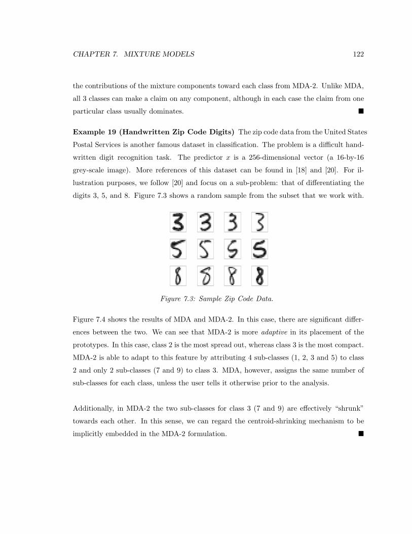
CHAPTER 7. MIXTURE MODELS 122
the contributions of the mixture components toward each class from MDA-2. Unlike MDA,
all 3 classes can make a claim on any component, although in each case the claim from one
particular class usually dominates.
Example 19 (Handwritten Zip Code Digits) The zip code data from the United States
Postal Services is another famous dataset in classification. The problem is a difficult hand-
written digit recognition task. The predictor x is a 256-dimensional vector (a 16-by-16
grey-scale image). More references of this dataset can be found in [18] and [20]. For il-
lustration purposes, we follow [20] and focus on a sub-problem: that of differentiating the
digits 3, 5, and 8. Figure 7.3 shows a random sample from the subset that we work with.
Figure 7.3: Sample Zip Code Data.
Figure 7.4 shows the results of MDA and MDA-2. In this case, there are significant differ-
ences between the two. We can see that MDA-2 is more adaptive in its placement of the
prototypes. In this case, class 2 is the most spread out, whereas class 3 is the most compact.
MDA-2 is able to adapt to this feature by attributing 4 sub-classes (1, 2, 3 and 5) to class
2 and only 2 sub-classes (7 and 9) to class 3. MDA, however, assigns the same number of
sub-classes for each class, unless the user tells it otherwise prior to the analysis.
Additionally, in MDA-2 the two sub-classes for class 3 (7 and 9) are effectively “shrunk”
towards each other. In this sense, we can regard the centroid-shrinking mechanism to be
implicitly embedded in the MDA-2 formulation.
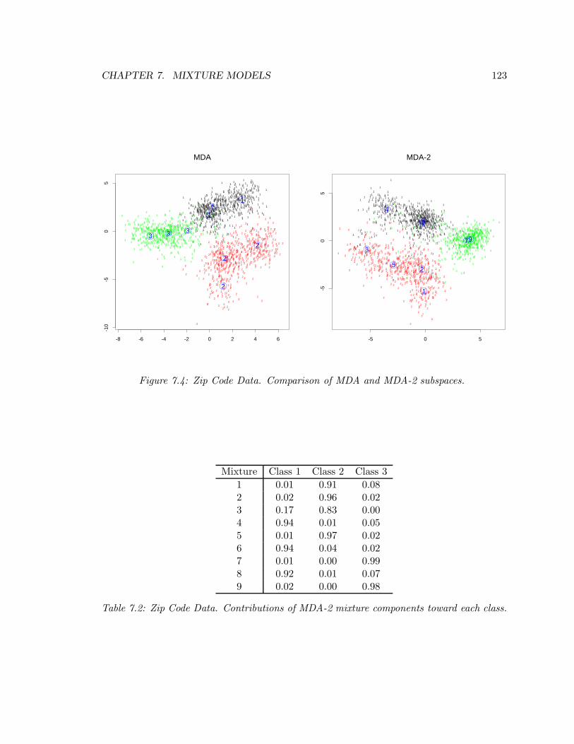
CHAPTER 7. MIXTURE MODELS 123
MDA
-8 -6 -4 -2 0 2 4 6
-10
-50
5
11 1
1
111
11 1
1
11
11
1
1
1
1
1
1
1
1
1
1
11
1
1
1
1
1
1
1
1
1
1
11
1
1
1
1
1
1
1
11
1
1 1
1
11
1
1
11
11
1
1
1
11
1
1
1
1
1
1
1
1
1
1
1
1
1
1
1
1
1
1
1
1
11
1
1
1
1
11
1
1
1
1
1
1
1
1
1
1
1
1
1
1
1
1
1
11
1
1
1
1
1
1
1
1 11
1
1
1
1
1
1
1
1
1
1
1
1
1
11
1
11
1
1
1
1
1
1
1 1
1
1
11
1
1
111
11
1
1
1
1
1
1
1 1
1
1
1
1
1
1
11
1
1 1 1
1
1
1
111
1 1
1
1
1
1
11
1
1
1
1
1
1
1
11
11
1
1
11
1
1
1
1
1
1
1
1
1
1
1
1
11
1
1
1
1
11
1
1
1
1
1 1
1
11
1
1
11
11
1
1
1
1
1
11 1
1
1
1
1
1
11
1
11
1
11
11
111
1 11
1
1
1
1
1
1
1
1
1
11
11
1 1
1
1
1
1
1
11
1
1
1
1
1
1
11
1
1
1
1 1
1
1
1
1
1
1
1
1 1
1
1
1
1
1
1
1
11
1
1 1
1
1
1
1
1
1
1
1
1
1
1 1
1
11
1
1
1
11
1
1
1
1
1
1
1
1
1
1
11
1
1
1
1
1
1
1
1
1
1
11
1
1
1
1
1
1
1
1
1 1
1
1
1
11
1
111
1
1
1
1 1
1
1
1
1
1
1
1
1
11
1
1
1 1
11
1
1
1
1
1
1
11
11
1
1
1
1
1
1
1
1
1
1
1
1
11
11
1
1
1
11
1
1
1
1
1
1
1
1
1
1
1
1
1
1
1
1
1
1
11
1
11
1
1
1
1
1
11
1
1
1
1
11
1
1
11
1
11
1
1
1
1
1
1
1
1
11
1
1
1
1
11
1
1
1 11
111
111
11
1
1
11
1
1
1
11
1
1
1
11
11
1
11
11
1
1
1
11
1
11
1
1
11
1
1
1
11
1
1
1
1
1
1
1
1
1
1
1
1
11
11
11
11
1
1
1
11
11
1
11 11
11
1 1
1
1
1
1
1
1
1
1
1
1
1
1
1
1
11
1
11
1
1
11
1
1
1
1
11
1
11
1
1
1
1
1
1
111
11
1
11
1
1
1
11
1
1
1
1
1
1
1
1
1
1 1
1
1
1
1
1
1
1
1
11
2
2
2
2
2
22
2
2
2
2
2
2
2
2
2
22
22
22
2
2
222
2
2
2
2
2
2
2
2
2
2
2
2
2
2
2
2
2
2
2
2
2
2
2
2
2
2
2
2
2
2
22
2
2
22
2
2
2
2
2
2
22
2
2
2
2
2
2
2
2
2
22
2
2
2
2
22
22
2
2
22
2
2
2
2
2
2
2
2
2
22
2
2
2
2
22
2
2
2
2
2
2
2
2
22
22
2
2
2
2
2
2
2
2
2
2
2
2
2
2
2
22
2
2
2
2
2
2
2
2 22
22
2
2
2
2
22
2
2
2
2
2
2
2
2
2
2
2
2
2
2
2
2
2
2
2
2
22
2
2
2
2
2
2
2
2
2
2
22
2
2
2
2
2
2
2
2
2
2 2
2
2
2
2
2
2
2
2
2
2
2
2
2
22
2
2
2
2
2
2
2
22
2
2
2
2
2
2
2
22
2
2
2
2
2
2
2
2
2
2
22
2
2
2
2
2
2
2
2
2
2
2
2
2
2
2
2
2 22
2
2
2
2
2
2
2
2
22
2
2
2
2
2
2
2
2
2
2
2
2 22 2
2
2
2
2
2
2
2
2
2
2
2
2
22
2
2
2
2
2
2
2
2
22
2
22
2
2
2
2
2
2
2
2
2
2
2
2
2
22
2
2
2
2
22
2
2 2
2
2
2
2
2
22
2
2
2
2
2
2
2
2
2
2
2
22
2
22
2
2
2
2
2
22
2
2
2
2
22
2
2
2
2
2
2
2
2
2
2
2
2
2
2
2
2
2
2
2
2
2
2
2
2
2
2
2
2
2
2
2
2
2
2
2
2
22
2
2
2
2
2
2
2
2
2
2
2 22
2
2
2
2
2
2
22
2
2
2
22
22
2
2
2
2
22
22
2
2
2
2
2
22
2
2
2
222
2
2
2
2
2
2
2
2
2
2
2
2
2
2
2
2
2
2
2
2
2
2
2
2
2
2
2
2
2 2
2
2
2
22
2
2
2
2
2
2
2 2
2
2
2
2
2
22
2
2
2
2
2
2
2
2
2
2
2
2 2
2
2
2
2
2
2
2
2
2
2
2
2
2
2
2
22
2
22
2
22
2
2
22 2
2
2
3
3
3
3
3
3
3
3
3
3
3
3
3
3 3
3
3
3
33
3
3
3
33
3
33
3
3
3
3
3
3
3
3
3
3
3
3
3
33
3
3
3
3 3
3
3
3
333
3
3
3
3
3
3
3
33
33
3
33
333
3
3
3
33
3
33
33
3
3
3
3
33
3
33
333
3
3
3
3
3
3
3
33
3
3
3
3
3
3
33
3
3
3
3
3
3
3
3
3
3
3
3
3
3
33
3
3
3
3
3
3
3 3
3
33 3
3
3
3
33
33
33
3
33
3
3
3
3
3
3
33
3
3
33
3
3
3
3
3
3
3
33
333 3
3
3
3
3
3
33
33
3 33
33
3
3
3
33
3
3
3
3
3
3
3
3
3 3
3
3
3
3
3
3
3
3
3
333
33
3
33
3
3
3
3
3
3
3
3
3
3
3
3
3
3
3
3
3
3
3
3
33
3
3
3
3
3
3
3
3
3
3
33
3
3 33
3
3
3
3
3
3
3
3
33
33
3
3
3
3
33
3
3
3
3
3
33
3
3
3
3
33
33
3
3
3
3
3 33 3
3
3
3
3
3
3
3
3
3
3
3
33
33
33
3
3
3
3
3
3
33
3 3
3 33
3
3 33
3
333
3 3
3
3
3
33
33
33
3
3 3
33
3
3
3
3
33
33
3
3
3
3
3
3 3
3
3
3
3
33
33
3
3
3
3 3
3
3
3
3
3
3
3
3
33
33 3 33
3
3
3
3
3
3
3
33
3
3
3
3
3
3
3
3
3
3
3
33
3
3
3
3
3
3
3 3
3
3
3
3
3
3
3
3
3
3
3
3
33
3
3
3
3
3
33
3
3
3
3 3
3
3
33
3 3
3
33
3
3
3
33
3
3
3
3
3
3
3
3
3
3
3
3
3
33
3
3
3
33
3
3
3
33
3
3
3
3
33
33
3 3
3
33
3
33
3
3
3
33
3
3
33
3
33
3
3
3 3
3
3 3
3
3
3
33 3
33
3
3
3
3
33
3333
MDA-2
-5 0 5
-50
5
1 1
1
1
1
1
11
11
1
111
1
1
1
1
1
1
1
1
11
1
1
1
1
1
1
1
11
1
1
1
1
1
1
1
1
1
11
1
1
1
11
1
1
1
1 1
1
1
11
11
1
1
1
11
1
1
1
1 1
1
1
1
1
1
1
1
1
1
1
1
1
1
1
1
1
1
1
1
1
1
1
1
1
1
1
1
1
1
1
1
1
1
1
1 11
1
1
1
11
1
1
1
1
1
1
1
1
1
1
1
1
1
1
1
1
1 1
1
1
1
11
1
1
11
1
1
1
1
1
1
1
1
1
1
1
11
1
1
1
111
1
1
1
1
1
1
1
11
1
11
1
1
1
11
1
11
1
1
11
11 1
1
1
11
1
1
1
1
1
11
1
1
1
1
1
1
11
1
11
1
11
11
1
1
1
11
1
1
1
11
1
1
1
1
1
1
1
1
1
11
1
1
1
1
11
1
1
1 1
1
1
1
1
1
1
11
1
1 1
1
1
1
1
1
1
11
1
1
1
1
1
1
1
1
1
1111
1
1
1
1
1
1
1
1
1
1
1
1
1
1
1
1
1
1
1
1
1
1
1
1
1
11
1
1
1
1
111
1
1
1
1
1 1
1
1
111
1
1
1
1
1 1
1
1
1
1
1
11
11
1
1
1
1
1
1
1 1 1
1
1 1
11
1
1
1
1
1
1
1
1
1
1
1
1
1
1
1
1
11
11
1
1
1
1
1
1
1
1
1
1
111
1
1 1
1
1
1
1
11
1
1
1
1
1
1
11
1
1
1
1
1
11
1
1
11
1
1
1
1
1
1
1
1
1
1
111
1
1
1
1
1 11
1
1
1
1
1 1 11
11
1
11
1
1
1
1
1
1
1
1
1
1
1
1
1
1
1
1
11
1
1
1
1
1
1
1
1
1
1
1
1
1
1
1
1
1
1
1
1
1
11
1
1
1
1
1
1
1
1
1
1
1
1
11
1
1
1
11
1
1
11
11
1
11
1
1
1
1
1
11
1
1
1
11
11
1
111
1 1
11
1
1
1
1
11
11 1
1
1
1
1
1
1
1
1
111
1
1
1
1
1
1
1
1
1
1
1
11
111
1
11
1
1
1
1
1
1
1
1
111
1
11
1
11
1
1
1
11 1
1
1
1
1
111
1
1
1
11
1
1
1
11
1
1
1
1
11
1 1
11
1
1
1
1
1
1
1 11
1
11
1
1
1
1
1
1
1
1
11
1
1
11
1
1
11
1
1
1
1
1
2
2
2
2
2
2
2
2
2
2
2
2
22
2
2
2
2
2
2
22
2
2
222
2
2
2
2
2
2
2
2
222
2
2
22
2
2
22
2
2
2
2
2
2
2
2
2
2
2
2
2
2
2
2
2
2
2
2
2
2
2
2
22
2
2
2
2
2
2
2
2
2
2
22
2
2
22
2 2
22
2 2
2
2
2
2
2
2
2
2
2
2 2
2
2
22
2
2
2
2
2
2
2
2
2
2
22
2
22
2
2
2
2
2
2
2
2
2
2
2 2
2
2
2
2
2
2
2
2
2
2
2
22
2
22
2
2
2
2
2
2
2
2
2
2
2
2
2
2
2
2
2
2
2
2
22
2
2
2
2
22
2
2
2
22 2
2
2
2
2
2
2
2
2
2
2
2
2
2
2
2
2
2
2
2
22
2
2
2
2
22
2
2
2
2
2
2
2
2
2
2
22
2
2
2
2
2
2
2
2
2
2 22
2
2
2
2
2
2
2
2
2
2
2
2
2
2
2
2
2
2
2
2
2
2
2
2
2
2
2
2
22
2
2
2
2
2
22
2
2
2
2
2
2
2
2
2
2
2
2
2
2 2
2
22
22
2
2
2 2
2
2
2
2
2
2
22
2
2
2
2
2
2
2
2
2
22
2
2
2
2
2
2
2222
2
2
2
2
2
2
22
2
2
2
2 2
2
2
2
2
2
2
2
2
22
2
2
2
2
2
2
2
2
2
2
22
2
2
22
22
22
22
22
2
2
2
2
2 2
2
2
2
2
2
2
2 2
2 2
2
2
2
2
2
2
2
2
2
2 2
22
2
2
2
2
2
2
2
2
2
2
2
2
2
2
2
2
2
2
22
2
2
2
2
22
2
2
2
2
2
2
2
2
2
2
2
2
22
2
2
2
2
2
2
2
2
22
2
2
2
2 2
2
2
2
2
2
2
2
22
2
2
2
2
2
22
2
2
2
2
2
2
2
2
2
2
2
2
2
2
2
2
2
2
2
2
2
2
2
2
2
2 2
2
2
2
2
2
2
2
2
2
22
2
2
2
2
2
2
2
2
2
2
2
2
2
2
2
2
2
2
2
22
2
2
2
2
2
2
2
2
2
2
2
2
2
2
2
2
2
22
2
2
2
2
3
3
3
3
3
3
3
3
3
3
33
3
33
3
3
3 33
3
3
3
33
3
33
3
33
3
3
3
33
3
3
33
3
3 3
33
3
3
3 3
33
3
3
3
3
3
3
33
3
3
33
33
3
3
3
33
3
3
3
3
33 3
3
3
33
3 33
3
3
3
3
3
3
3 3
3
3
3
33
33
33
3
3
3
3
3
3
3
33
3
3
3 3
3
3
3
3
3 3
3
3
3
3
33
3
3
3
3
3 3
33
3
3
3
3
33
3
333
3 33
3
3
3
33
3
3
3
3
33
33
3
3
3
3
3
3
3
3
33
33
3
3
3
3
3
3
3
3
3
3
3
3
3
3
33
3
3
3
3
33
3
3
3
3 3
3 3
3
3
3
3
3
3
3
3
33
3
3 33
33
3 3
33
33
33
3
3
3
3
3
3
3
3
3
3
33
3
3
3
3
3
33
3
3
3
3
3
3
33
3
3
3
3
3
3
3
3
3
3
3
3
3
3
3
3
3
3
3
3
3
3
3 3
33
3
3
3
3
3
3
3
3
3 3
33 3
3
3 3
3
3
3
3
33
3
3
33
3
3
3
3
3
3
3
3 3
3
33
3
3
3
3
3
3
3
33 3
3
3
33
3
3
33
3
3
3 3
3
33
3
3
3
3
33
33
3
33
3
3
3
3
33
33
33
3
33
3
3
33
3
3
3
3
3
3
3
3 33
3
33
33
3
3
333
3
33
3
33 3
3
3
3
3
3
3
3
33
3
3
33
33
33
3
3
33
3
3
3
3
3
3
33
33
33
3
3
3
33
3
3
33
3
3
3
33
33
3
3
33
3
33
3
3
3
3
3
3
3
3
3
3
3
3
33
33
3
333
3 3
3
3
33
3
3
333
3 33
3
3
3
3
3
3
3
3
33
3
3
33
3333
3
3
3
3
3
3
3
3
3
3
3
3 3
3
3
3
3
3
3
3
3
33
3
3
3
3
3
3
3
333
3
3
33
3
1
2
3
4
5
6
7
8
9
Figure 7.4: Zip Code Data. Comparison of MDA and MDA-2 subspaces.
Mixture Class 1 Class 2 Class 3
1 0.01 0.91 0.082 0.02 0.96 0.023 0.17 0.83 0.004 0.94 0.01 0.055 0.01 0.97 0.026 0.94 0.04 0.027 0.01 0.00 0.998 0.92 0.01 0.079 0.02 0.00 0.98
Table 7.2: Zip Code Data. Contributions of MDA-2 mixture components toward each class.

CHAPTER 7. MIXTURE MODELS 124
7.6 Aspect Model with Covariates
The new (and more adaptive) mixture model (7.4.2) actually corresponds to a natural
extension of the aspect model which we introduced in chapter 1. In section 1.4, we introduced
the problem of analyzing co-occurrence data with covariates. How can the aspect model
(section 1.3) be generalized to deal with this new problem? When each ξi (e.g., a customer,
or a geographical site) is associated with a vector of covariates, xi ∈ Rd, a natural way to
extend the concept of the occurrence probability, p(ξi), is to introduce a density function
for the covariates, p(xi). Then, the aspect model
P (ξi, ηk) =∑
α
p(ξi|cα)P (ηk|cα)P (cα)
simply becomes
P (xi, y = k) =∑
α
p(xi|cα)P (y = k|cα)P (cα),
where, to conform to the standard notation in the context of discriminant analysis, we have
used the event y = k to denote the occurrence of ηk. If we further assume that the con-
ditional density of x given α is Gaussian with a common covariance matrix for all α, i.e.,
p(x|α) = φ(x;µα,Σ), then we obtain exactly the same mixture model as equation (7.4.2).
This brings us back to our discussion in chapter 2. A critical message from chapter 2
is that the constrained ordination problem for co-occurrence data with covariates is equiv-
alent to LDA. MDA is, of course, another generalization of LDA. In section 1.3, we intro-
duced Hofmann’s aspect model as a more probabilistically oriented model for co-occurrence
data, which, instead of assigning scores for the ξi’s and ηk’s, models the probabilities of
co-occurrence P (ξi, ηk) directly. Hence, it is no surprise that MDA should correspond to an
extension of Hofmann’s aspect model.

CHAPTER 7. MIXTURE MODELS 125
7.7 Summary
Everything has now come back together. Recall that we started this thesis with the anal-
ysis of co-occurrence data. We then left co-occurrence data to focus on a related problem,
namely, discriminant analysis. We pushed discriminant analysis a long way in the non-
parametric direction. Then, in this chapter, we came back from non-parametric models to
an approximation using mixtures of Gaussians. And, finally, from the mixture models, we
were brought back to the problem of co-occurrence data, with which we started our journey.
It was a very rich journey that we just went on. Because of such richness, not every issue
could be addressed with the same level of detail in a thesis — or else I would remain a
graduate student for a very long time.
Some problems we studied with great care, such as in chapters 4, 5 and 6. There, we
studied feature extraction in its utmost generality (without any parametric assumptions at
all) and investigated ways to incorporate the feature extraction component into probabilis-
tic models for non-parametric discriminant analysis. We went into technical details and
made various new contributions.
Chapters 1, 2, 3 and 7 contain methodological reviews, as well as our insights that bring
together two important problems in multivariate statistics, each rich in itself and having
largely evolved along its own path — the analysis of co-occurrence data and discriminant
analysis. The connections we’ve made are relatively novel and not widely known and,
therefore, become another important — though less technical — contribution of this thesis.
Because of these insights, research areas that have previously developed independently of
one another can now come together!

Appendix A
Eigenvalue Problems
In this appendix, we provide a very brief but systematic overview of several classic multi-
variate techniques. More details can be found in [30].
A.1 The Basic Eigenvalue Problem
Most classic multivariate techniques, such as principal components, canonical correlations,
and linear discriminant analysis, can be reduced to solving the following optimization prob-
lem: Let S be an M -by-M positive-definite and symmetric matrix and let α ∈ RM ; find
the optimal α that
max‖α‖=1
αT Sα.
By the spectral decomposition of S, we obtain S = V DV T , where V is an orthonormal
matrix whose column vectors are the eigenvectors of S, and D = diag(d1, d2, ..., dM ) is a
diagonal matrix whose diagonal elements are the eigenvalues of S such that d1 ≥ d2 ≥ ... ≥dM . Let β = V T α; then ‖β‖ = 1 because orthogonal transformations preserve lengths.
Therefore, the problem is equivalent to
max‖β‖=1
βT Dβ.
126

APPENDIX A. EIGENVALUE PROBLEMS 127
But since D is a diagonal matrix, we have
βT Dβ =
M∑
m=1
β2mdm.
Recall ‖β‖2 =∑M
m=1 β2m = 1. Hence it is clear that the maximum is achieved at β∗ =
(1, 0, 0, ..., 0)T . The optimal α, therefore, is given by
α∗ = V β∗ = v1,
the eigenvector of S corresponding to the largest eigenvalue, or the first eigenvector.
A.2 The Generalized Eigenvalue Problem
In the basic problem, the constraint on α is ‖α‖ = 1, where ‖ · ‖ is the Euclidean norm
‖α‖2 = αT α. A more general problem is to use a different norm on α — e.g., αT Θα —
where Θ is another positive-definite symmetric matrix. The problem then becomes
maxαT Θα=1
αT Sα
Let β = Θ1/2α. This problem can then be equivalently turned into
max‖β‖=1
βT(
Θ−1/2SΘ−1/2)
β.
From section A.1, we know that the optimal β is the first eigenvector of Θ−1/2SΘ−1/2. As
an eigenvector, it must satisfy
(
Θ−1/2SΘ−1/2)
β = λβ,
(
Θ−1S)
(
Θ−1/2β)
= λ(
Θ−1/2β)
,
which indicates that Θ−1/2β is an eigenvector of Θ−1S with the same eigenvalue. But as
α = Θ−1/2β, the optimal α is the first eigenvector of Θ−1S. An alternative argument based
on the concept of weighted Euclidean spaces is provided in [17].
APPENDIX A. EIGENVALUE PROBLEMS 128
A.3 Principal Components
Suppose x is a random vector in RM with distribution F ; the principal component is defined
to be the direction of the largest variance, i.e.,
argmax‖α‖=1
var(αT x) = argmax‖α‖=1
αT Σα,
where Σ is the covariance matrix for F . By section A.1, the largest principal component is
simply the first eigenvector of the covariance matrix.
A.4 Linear Discriminant Analysis
Let B be the between-class covariance matrix and W , the within-class covariance matrix;
the linear discriminant direction is the solution of the following problem (see [30] and chapter
2 of this thesis):
maxα
αT Bα
αT Wα,
which is the same as
maxαT Wα=1
αT Bα.
By section A.2, it follows that the best linear discriminant direction is the first eigenvector
of W−1B.

Appendix B
Numerical Optimization
In this appendix, we provide a very brief overview of the standard numerical optimization
techniques. Numerical optimization is a basic building block for maximizing LR(α), the
fundamental problem of this thesis. Throughout the thesis, we have chosen to suppress the
details of our implementation so as to focus on the main statistical ideas. In general, our
implementation follows the basic guidelines outlined below.
B.1 The Generic Optimization Algorithm
Suppose x ∈ Rd, and we want to minimize F (x), where F (x) has continuous second deriva-
tives:
minx
F (x).
Note that it suffices to just consider minimization problems because
maxx
F (x) ⇐⇒ minx− F (x).
The general strategy is to start at an initial point x0 and move in a series of descent directions
toward the minimum. Let g(x) be the gradient of F (x), i.e.,
g(x) =∂F
∂x.
129

APPENDIX B. NUMERICAL OPTIMIZATION 130
The generic descent algorithm is given in algorithm B.1. Specific algorithms differ in how
Algorithm B.1 Generic Descent Algorithm.
• Let r = 0.
• Repeat
1. Find a descent direction at xr, pr, such that pTr gr < 0.
2. Choose a step-size along pr, e.g.,
ar = argmina
F (xr + apr).
3. Move to xr+1 = xr + arpr.
4. Increment r = r + 1.
Until convergence.
they select the descent direction, pr, at each iteration.
B.2 Choice of Descent Direction
B.2.1 Steepest Descent
One option is to choose p = −g, so that we are moving in the fastest-decreasing direction
of the function. This method is called the steepest descent method. However, it does not
use any second-order information of the function and can be relatively inefficient.
B.2.2 Newton’s Method
The most popular method that takes advantage of second-order information is Newton’s
method and its numerous variations. Let H(x) be the Hessian matrix of F , i.e.,
H(x) =∂2F
∂x∂xT.
Newton’s method chooses p = −H−1g. Note this is guaranteed to be a descent direction if
H is positive definite, because pT g = gT p = −gT H−1g < 0.

APPENDIX B. NUMERICAL OPTIMIZATION 131
But if H is not positive definite, then p is not guaranteed to be a descent direction. In
this situation, modifications of H are necessary. For example, we can choose some λ > 0
and use
p = −(H + λI)−1g.
Another variation, called quasi-Newton method, is to use some other matrix G that is
positive-definite and behaves like a Hessian. The quais-Newton method is very popular
because evaluating the actual Hessian can often be computationally expensive or simply
impossible. There are different algorithms for constructing the matrix G at each iteration.
However, we will not go into any of the details here. More details can be found in [16].
B.3 Choice of Step Size
Once a descent direction is fixed, finding the step-size is a (relatively simple) univariate
problem. Various line-search methods can be used to solve this problem, such as the golden-
section search, which is what we implemented for this thesis. Again, we omit the details
and refer the readers to [16]. We only point out that it is not absolutely necessary to pick
ar = argmina
F (xr + apr)
exactly at each step. Usually it suffices to pick ar which guarantees that the function is
decreasing; i.e., ar must satisfy
F (xr + arpr) < F (xr).

Appendix C
Density Estimation
Another basic building block for maximizing LR(α) is that we must be able to estimate a
univariate density function and its first two derivatives (see section 4.4).
C.1 Kernel Density Estimation
Suppose z1, z2, ..., zn ∼ F , where F is a probability distribution. Suppose there exists a
density function f for F . Let w be a kernel function such that
∫ ∞
−∞w(z)dz = 1,
∫ ∞
−∞zw(z)dz = 0 and
∫ ∞
−∞z2w(z)dz <∞;
then it is well-known (see e.g., [36]) that
f(z) =1
nb
n∑
i=1
w
(
z − zi
b
)
is a consistent estimator of f . Moreover,
f′
(z) =1
nb2
n∑
i=1
w′
(
z − zi
b
)
and f′′
(z) =1
nb3
n∑
i=1
w′′
(
z − zi
b
)
are consistent estimators of f′
and f′′
, respectively.
132
APPENDIX C. DENSITY ESTIMATION 133
C.2 The Locfit Package in Splus
Based on the theory of local likelihood (see [39]), the Locfit package in Splus is a recent
development due to Clive Loader [29], and it is the package that we used in our implemen-
tation. Local likelihood estimates have some advantages over plain-vanilla kernel estimates;
e.g., the automatic elimination of boundary bias to the first order (see e.g., [14]), etc. We
choose not to go into the theory of local likelihood estimation here. Most density estimation
methods, including local likelihood, have an equivalent kernel representation and, therefore,
can be viewed as a special kernel estimator, at least on the conceptual level.
The choice of Locfit as our density estimation module, however, is largely pragmatic.
Locfit implements a rather elaborate set of evaluation structures and interpolation strate-
gies — the density function is only evaluated at a few strategically selected points, and
its values at other points are obtained by interpolation, thereby significantly reducing the
amount of computation time. For more details, we refer the reader to section 12.2 of [29].
It is also worth pointing out that for density estimation, one must use the Locfit package
with great care. Locfit uses the log-link as its default, and the derivatives it returns are
for g = log(f) rather than the for the original f . Hence one obtains g′
and must use
f′
= g′ × f
to obtain the correct derivative. Similarly, for the second derivative, one must rely on
f′′
=g′′
f2 + (f′
)2
f.
Details are available in section 6.1.2. of [29].

Bibliography
[1] Bensmail, H. and Celeux, G. Regularized Gaussian Discriminant Analysis Through
Eigenvalue Decomposition. Journal of the American Statistical Association, 91(436),
Dec. 1996.
[2] Breiman, L., Friedman, J. H., Olshen, R. A., and Stone, C. J. Classification and
Regression Trees. Wadsworth, 1984.
[3] Brieman, L. Bagging Predictors. Machine Learning, 24, 1996.
[4] Cook, R. D. and Weisberg, S. Discussion of Li (1991). Journal of the American
Statistical Association, 86, 1991.
[5] Cook, R. D. and Yin, X. Dimension Reduction and Visualization in Discriminant
Analysis. To appear in the Australian and New Zealand Journal of Statistics, 2001.
[6] Devijver, P. A. and Kittler, J. Pattern Recognition: A Statistical Approach. Prentice-
Hall International, 1982.
[7] Diaconis, P. and Shahshahani, M. On Nonlinear Functions of Linear Combinations.
SIAM Journal on Scientific and Statistical Computing, 5, 1984.
[8] Fisher, R. A. The Use of Multiple Measurements in Taxonomic Problems. Annals of
Eugenics, 7(Part II), 1936.
[9] Flury, B. Common Principal Components and Related Multivariate Models. Wiley,
1988.
[10] Friedberg, S. H., Insel, A. J., and Spence, L. E. Linear Algebra. Prentice Hall, 1989.
134
BIBLIOGRAPHY 135
[11] Friedman, J. H. Exploratory Projection Pursuit. Journal of the American Statistical
Association, 82(397), Mar. 1987.
[12] Friedman, J. H. Regularized Discriminant Analysis. Journal of the American Statistical
Association, 84(405), Mar. 1989.
[13] Friedman, J. H., Hastie, T. J., and Tibshirani, R. J. Additive Logistic Regression: A
Statistical View of Boosting. The Annals of Statistics, 28(2), 2000.
[14] Friedman, J. H., Hastie, T. J., and Tibshirani, R. J. The Elements of Statistical
Learning: Prediction, Inference and Data-Mining. Springer-Verlag, to appear in 2001.
[15] Friedman, J. H., Stuetzle, W., and Schroener, A. Projection Pursuit Density Estima-
tion. Journal of the American Statistical Association, 79(387), Sept. 1984.
[16] Gill, P. E., Murray, W., and Wright, M. H. Practical Optimization. Academic Press,
1981.
[17] Greenacre, M. J. Theory and Applications of Correspondence Analysis. Academic
Press, 1984.
[18] Hastie, T. J., Buja, A., and Tibshirani, R. J. Penalized Discriminant Analysis. The
Annals of Statistics, 23(1), 1995.
[19] Hastie, T. J. and Tibshirani, R. J. Generalized Additive Models. Chapman and Hall,
1990.
[20] Hastie, T. J. and Tibshirani, R. J. Discriminant Analysis by Gaussian Mixtures.
Journal of the Royal Statistical Society (Ser. B), 58, 1996.
[21] Hastie, T. J., Tibshirani, R. J., and Buja, A. Flexible Discriminant Analysis by Optimal
Scoring. Journal of the American Statistical Association, 89(428), Dec. 1994.
[22] Hastie, T. J., Tibshirani, R. J., and Buja, A. Flexible Discriminant and Mixture
Models. In J. Kay and D. Titterington, editors, Proceedings of Neural Networks and
Statistics Conference, Edinburgh, 1995. Oxford University Press.

BIBLIOGRAPHY 136
[23] Hill, M. O. Correspondence Analysis: A Neglected Multivariate Method. Applied
Statistics, 23, 1974.
[24] Hofmann, T. and Puzicha, J. Statistical Models for Co-occurence Data. Technical
Report A.I. Memo No. 1625, M.I.T., 1998.
[25] Huber, P. J. Projection Pursuit. The Annals of Statistics, 13(2), June 1985.
[26] James, G. Majority-Vote Classifiers: Theory and Applications. Ph.D. dissertation,
Stanford University, 1998.
[27] Johnson, K. W. and Altman, N. S. Canonical Correspondence Analysis as an Approx-
imation to Gaussian Ordination. Environmetrics, 10, 1999.
[28] Li, K. C. Sliced Inverse Regression for Dimension Reduction. Journal of the American
Statistical Association, 86, 1991.
[29] Loader, C. Local Regression and Likelihood. Springer-Verlag, 1999.
[30] Mardia, K. V., Kent, J. T., and Bibby, J. M. Multivariate Analysis. Academic Press,
1979.
[31] McCullagh, P. and Nelder, J. A. Generalized Linear Models. Chapman and Hall, 1983.
[32] Polzehl, J. Projection Pursuit Discriminant Analysis. Computational Statistics and
Data Analysis, 20, 1995.
[33] Ripley, B. D. Pattern Recognition and Neural Networks. Cambridge University Press,
1996.
[34] Roosen, C. and Hastie, T. J. Logistic Response Projection Pursuit. Technical Report
BLO11214-930806-09TM, AT&T Bell Laboratories, 1991.
[35] Rubenstein, Y. D. Discriminative vs. Informative Classification. Ph.D. dissertation,
Stanford University, 1998.
[36] Silverman, B. Density Estimation for Statistics and Data Analysis. Chapman and
Hall, 1986.

BIBLIOGRAPHY 137
[37] ter Braak, C. J. F. Correspondence Analysis of Incidence and Abundance Data: Prop-
erties in Terms of a Unimodal Response Model. Biometrics, 41, Dec. 1985.
[38] ter Braak, C. J. F. Canonical Correspondence Analysis: A New Eigenvector Technique
for Multivariate Direct Gradient Analysis. Ecology, 67(5), 1986.
[39] Tibshirani, R. J. Local Likelihood Estimation. Ph.D. dissertation, Stanford University,
1984.