feature embedding for dependency parsing
TRANSCRIPT

Proceedings of COLING 2014, the 25th International Conference on Computational Linguistics: Technical Papers,pages 816–826, Dublin, Ireland, August 23-29 2014.
Feature Embedding for Dependency Parsing
Wenliang Chen†, Yue Zhang‡, and Min Zhang†∗†School of Computer Science and Technology, Soochow University, China
‡Singapore University of Technology and Design, Singapore{wlchen, mzhang}@suda.edu.cn
Abstract
In this paper, we propose an approach to automatically learning feature embeddings to addressthe feature sparseness problem for dependency parsing. Inspired by word embeddings, featureembeddings are distributed representations of features that are learned from large amounts ofauto-parsed data. Our target is to learn feature embeddings that can not only make full use ofwell-established hand-designed features but also benefit from the hidden-class representationsof features. Based on feature embeddings, we present a set of new features for graph-baseddependency parsing models. Experiments on the standard Chinese and English data sets showthat the new parser achieves significant performance improvements over a strong baseline.
1 Introduction
Discriminative models have become the dominant approach for dependency parsing (Nivre et al., 2007;Zhang and Clark, 2008; Hatori et al., 2011). State-of-the-art accuracies have been achieved by the use ofrich features in discriminative models (Carreras, 2007; Koo and Collins, 2010; Bohnet, 2010; Zhang andNivre, 2011). While lexicalized features extracted from non-local contexts enhance the discriminativepower of parsers, they are relatively sparse. Given a limited set of training data (typically less than 50ksentences for dependency parsing), the chance of a feature occurring in the training data but not in thetest data can be high.
Another limitation on features is that many are typically derived by (manual) combination of atomicfeatures. For example, given the head word (wh) and part-of-speech tag (ph), dependent word (wd)and part-of-speech tag (pd), and the label (l) of a dependency arc, state-of-the-art dependency parserscan have the combined features: [wh; ph], [wh; ph; wd; pd], [wh; ph; wd], and so on, in addition to theatomic features: [wh], [ph], etc. Such combination is necessary for high accuracies because the dominantapproach uses linear models, which can not capture complex correlations between atomic features.
We tackle the above issues by borrowing solutions from word representations, which have been in-tensely studied in the NLP community (Turian et al., 2010). In particular, distributed representations ofwords have been used for many NLP problems, which represent a word by information from the wordsit frequently co-occurs with (Lin, 1997; Curran, 2005; Collobert et al., 2011; Bengio, 2009; Mikolovet al., 2013b). The representation can be learned from large amounts of raw sentences, and hence usedto reduce OOV rates in test data. In addition, since the representation of each word carries informationabout its context words, it can also be used to calculate word similarity (Mikolov et al., 2013a), or usedas additional semantic features (Koo et al., 2008).
In this paper, we show that a distributed representation can be learned for features also. Learnedfrom large amount of automatically parsed data, the representation of each feature can be defined on the
∗Corresponding authorThis work is licenced under a Creative Commons Attribution 4.0 International License. Page numbers and proceedings footerare added by the organizers. License details: http://creativecommons.org/licenses/by/4.0/
816

features it frequently co-occurs with. Similar to words, the feature representation can be used to reducethe rate of unseen features in test data, and to capture inherent correlations between features. Borrowingterminologies from word embeddings, we call the feature representation feature embeddings.
Compared with the task of learning word embeddings, the task of learning feature embeddings ismore difficult because the size of features is much larger than the vocabulary size and tree structuresare more complex than word sequences. This requires us to find an effective embedding format and anefficient inference algorithm. Traditional LSA and RNN (Collobert et al., 2011; Bengio, 2009) modelsturn out to be very slow for feature embeddings. Recently, Mikolov et al. (2013a) and Mikolov et al.(2013b) introduce efficient models to learn high-quality word embeddings from extremely large amountsof raw text, which offer a possible solution to the efficiency issue of learning feature embeddings. Weadapt their approach for learning feature embeddings, showing how an unordered feature context canbe used to learn the representation of a set of complex features. Using this method, a large numberof embeddings are trained from automatically parsed texts, based on which a set of new features aredesigned and incorporated into a graph-based parsing model (McDonald and Nivre, 2007).
We conduct experiments on the standard data sets of the Penn English Treebank and the Chinese Tree-bank V5.1. The results indicate that our proposed approach significantly improves parsing accuracies.
2 Background
In this section, we introduce the background of dependency parsing and build a baseline parser based onthe graph-based parsing model proposed by McDonald et al. (2005).
2.1 Dependency parsingGiven an input sentence x = (w0, w1, ..., wi, ..., wm), where w0 is ROOT and wi (i = 0) refers to aword, the task of dependency parsing is to find y∗ which has the highest score for x,
y∗ = arg maxy∈Y (x)
score(x, y)
where Y (x) is the set of all the valid dependency trees for x. There are two major models (Nivreand McDonald, 2008): the transition-based model and graph-based model, which showed comparableaccuracies for a wide range of languages (Nivre et al., 2007; Bohnet, 2010; Zhang and Nivre, 2011;Bohnet and Nivre, 2012). We apply feature embeddings to a graph-based model in this paper.
2.2 Graph-based parsing modelWe use an ordered pair (wi, wj) ∈ y to define a dependency relation in tree y from word wi to word wj
(wi is the head and wj is the dependent), and Gx to define a graph that consists of a set of nodes Vx ={w0, w1, ..., wi, ..., wm} and a set of arcs (edges) Ex = {(wi, wj)|i = j, wi ∈ Vx, wj ∈ (Vx − {w0})}.The parsing model of McDonald et al. (2005) searches for the maximum spanning tree (MST) in Gx.
We denote Y (Gx) as the set of all the subgraphs of Gx that are valid spanning trees (McDonald andNivre, 2007). The score of a dependency tree y ∈ Y (Gx) is the sum of the scores of its subgraphs,
score(x, y) =∑g∈y
score(x, g) =∑g∈y
f(x, g) · w (1)
where g is a spanning subgraph of y, which can be a single arc or adjacent arcs, f(x, g) is a high-dimensional feature vector based on features defined over g and x, and w refers to the weights for thefeatures. In this paper we assume that a dependency tree is a spanning projective tree.
2.3 Baseline parserWe use the decoding algorithm proposed by Carreras (2007) and use the Margin Infused Relaxed Al-gorithm (MIRA) (Crammer and Singer, 2003; McDonald et al., 2005) to train feature weights w. Weuse the feature templates of Bohnet (2010) as our base feature templates, which produces state-of-the-artaccuracies. We further extend the features by introducing more lexical features to the base features. The
817

First-order[wp]h, [wp]d, d(h, d)[wp]h, d(h, d)wd, pd, d(h, d)[wp]d, d(h, d)wh, ph, wd, pd, d(h, d)ph, wh, pd, d(h, d)wh, wd, pd, d(h, d)wh, ph, [wp]d, d(h, d)ph, pb, pd, d(h, d)ph, ph+1, pd−1, pd, d(h, d)ph−1, ph, pd−1, pd, d(h, d)ph, ph+1, pd, pd+1, d(h, d)ph−1, ph, pd, pd+1, d(h, d)Second-orderph, pd, pc, d(h, d, c)wh, wd, cw, d(h, d, c)ph, [wp]c, d(h, d, c)pd, [wp]c, d(h, d, c)
Second-order (continue)wh, [wp]c, d(h, d, c)wd, [wp]c, d(h, d, c)[wp]h, [wp]h+1, [wp]c, d(h, d, c)[wp]h−1, [wp]h, [wp]c, d(h, d, c)[wp]h, [wp]c−1, [wp]c, d(h, d, c)[wp]h, [wp]c, [wp]c+1, d(h, d, c)[wp]h−1, [wp]h, [wp]c−1, [wp]c, d(h, d, c)[wp]h, [wp]h+1, [wp]c−1, [wp]c, d(h, d, c)[wp]h−1, [wp]h, [wp]c, [wp]c+1, d(h, d, c)[wp]h, [wp]h+1, [wp]c, [wp]c+1, d(h, d, c)[wp]d, [wp]d+1, [wp]c, d(h, d, c)[wp]d−1, [wp]d, [wp]c, d(h, d, c)[wp]d, [wp]c−1, [wp]c, d(h, d, c)[wp]d, [wp]c, [wp]c+1, d(h, d, c)[wp]d, [wp]d+1, [wp]c−1, [wp]c, d(h, d, c)[wp]d, [wp]d+1, [wp]c, [wp]c+1, d(h, d, c)[wp]d−1, [wp]d, [wp]c−1, [wp]c, d(h, d, c)[wp]d−1, [wp]d, [wp]c, [wp]c+1, d(h, d, c)
Table 1: Base feature templates.
base feature templates are listed in Table 1, where h and d refer to the head, the dependent, respectively,c refers to d’s sibling or child, b refers to the word between h and d, +1 (−1) refers to the next (previous)word, w and p refer to the surface word and part-of-speech tag, respectively, [wp] refers to the surfaceword or part-of-speech tag, d(h, d) is the direction of the dependency relation between h and d, andd(h, d, c) is the directions of the relation among h, d, and c.
We train a parser with the base features and use it as the Baseline parser. Defining fb(x, g) as the basefeatures and wb as the corresponding weights, the scoring function becomes,
score(x, g) = fb(x, g) · wb (2)
3 Feature Embeddings
Our goal is to reduce the sparseness of rich features by learning a distributed representation of features,which is dense and low dimensional. We call the distributed feature representation feature embeddings.In the representation, each dimension represents a hidden-class of the features and is expected to capturea type of similarities or share properties among the features.
The key to learn embeddings is making use of information from a local context, and to this endvarious methods have been proposed for learning word embeddings. Lin (1997) and Curran (2005) usethe count of words in a surrounding word window to represent distributed meaning of words. Brownet al. (1992) uses bigrams to cluster words hierarchically. These methods have been shown effectiveon words. However, the number of features is much larger than the vocabulary size, which makes itinfeasible to apply them on features. Another line of research induce word embeddings using neurallanguage models (Bengio, 2008). However, the training speed of neural language models is too slow forthe high dimensionality of features. Mikolov et al. (2013b) and Mikolov et al. (2013a) introduce efficientmethods to directly learn high-quality word embeddings from large amounts of unstructured raw text.Since the methods do not involve dense matrix multiplications, the training speed is extremely fast.
We adapt the models of Mikolov et al. (2013b) and Mikolov et al. (2013a) for learning feature embed-dings from large amounts of automatically parsed dependency trees. Since feature embeddings have ahigh computational cost, we also use Negative sampling technique in the learning stage (Mikolov et al.,2013b). Different from word embeddings, the input of our approach is features rather than words, andthe feature representations are generated from tree structures instead of word sequences. Consequently,
818

Figure 1: An example of one-step context. Figure 2: One-step surrounding features.
we give a definition of unordered feature contexts and adapt the algorithms of Mikolov et al. (2013b) forfeature embeddings.
3.1 Surrounding feature context
The most important difference between features and words is the contextual structure. Given a sentencex =w1, w2, ..., wn and its dependency tree y, we define the M -step context as a set of relations reachablewithin M steps from the current relation. Here one step refers to one dependency arc. For instance, theone-step context includes the surrounding relations that can be reached in one arc, as shown in Figure 1.In the figure, for the relation between “with” and “fork”, the relation between “ate” and “with” is in theone-step context, while the relation between “He” and “ate” is in the two-step context because it can bereached via the arc between “ate” and “with”. A larger M results in more contextual features and thusmight lead to a more accurate embedding, but at the expense of training speed.
Based on the M -step context, we use surrounding features to represent the features on the currentdependency relations. The surrounding features are defined on the relations in the M -step context. Take1-step context as an example. Figure 2 shows the representations for the current relation between “with”and “fork” in Figure 1. Given the current relation and the relations in its one-step context, we generatethe features based on the base feature templates. In Figure 2 the current feature “f1:with, fork, R”can be represented by the surrounding features “cf1:ate, with, R” and “cf1: fork, a, L” based on thetemplate “T1:wh, wd, d(h, d)”. Similarly, all the features on the current relation are represented by thefeatures on the relations in the one-step context. To reduce computational cost, we generate for everyfeature its contextual features based on the same feature template. As a result, the embeddings for eachfeature template is trained separately. In the experiments, we use one-step context for learning featureembeddings.
3.2 Feature Embedding model
We adapt the models of Mikolov et al. (2013b) and Mikolov et al. (2013a) to infer feature embeddings(FE). Based on the representation of surrounding context, the input to the learning models is a set offeatures and the output is feature embeddings as shown in Figure 3. For each dependency tree in largeamounts of auto-parsed data, we generate the base features and associate them with their surroundingcontextual features. Then all the base features are put into a set, which is used as the training instancesfor learning models.
In the embedding model, we use the features on the current dependency arc to predict the surround-ing features, as shown in Figure 4. Given sentences and their corresponding dependency trees Y , theobjective of the model is to maximize the conditional log-likelihood of context features,∑
y∈Y
∑f∈Fy
∑cf∈CFf
log(p(cf |f)) (3)
819
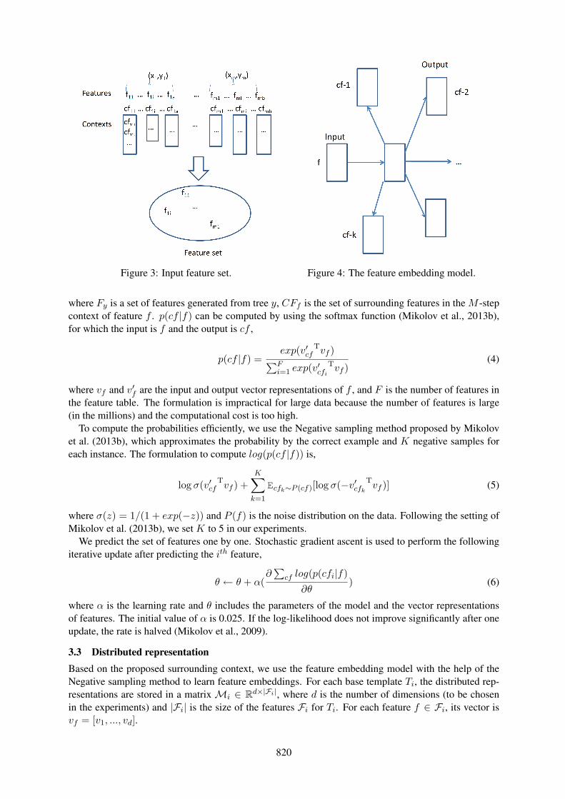
Figure 3: Input feature set. Figure 4: The feature embedding model.
where Fy is a set of features generated from tree y, CFf is the set of surrounding features in the M -stepcontext of feature f . p(cf |f) can be computed by using the softmax function (Mikolov et al., 2013b),for which the input is f and the output is cf ,
p(cf |f) =exp(v′cf
Tvf )∑Fi=1 exp(v′cfi
Tvf )(4)
where vf and v′f are the input and output vector representations of f , and F is the number of features inthe feature table. The formulation is impractical for large data because the number of features is large(in the millions) and the computational cost is too high.
To compute the probabilities efficiently, we use the Negative sampling method proposed by Mikolovet al. (2013b), which approximates the probability by the correct example and K negative samples foreach instance. The formulation to compute log(p(cf |f)) is,
log σ(v′cfTvf ) +
K∑k=1
Ecfk∼P (cf)[log σ(−v′cfk
Tvf )] (5)
where σ(z) = 1/(1 + exp(−z)) and P (f) is the noise distribution on the data. Following the setting ofMikolov et al. (2013b), we set K to 5 in our experiments.
We predict the set of features one by one. Stochastic gradient ascent is used to perform the followingiterative update after predicting the ith feature,
θ ← θ + α(∂
∑cf log(p(cfi|f)
∂θ) (6)
where α is the learning rate and θ includes the parameters of the model and the vector representationsof features. The initial value of α is 0.025. If the log-likelihood does not improve significantly after oneupdate, the rate is halved (Mikolov et al., 2009).
3.3 Distributed representationBased on the proposed surrounding context, we use the feature embedding model with the help of theNegative sampling method to learn feature embeddings. For each base template Ti, the distributed rep-resentations are stored in a matrixMi ∈ Rd×|Fi|, where d is the number of dimensions (to be chosenin the experiments) and |Fi| is the size of the features Fi for Ti. For each feature f ∈ Fi, its vector isvf = [v1, ..., vd].
820

< j : T (f) · Φ(vj) > for j ∈ [1, d]< j : T (f) · Φ(vj), wh > for j ∈ [1, d]
Table 2: FE-based templates.
4 Parsing with feature embeddings
In this section, we discuss how to apply the feature embeddings to dependency parsing.
4.1 FE-based feature templatesThe base parsing model contains only binary features, while the values in the feature embedding repre-sentation are real numbers that are not in a bounded range. If the range of the values is too large, they willexert much more influence than the binary features. To solve this problem, we define a function Φ(vi)(details are given in Section 4.3) to convert real values to discrete values. The vector vf = [v1, ..., vd] isconverted into vN
f = [Φ(v1), ...,Φ(vd)].We define a set of new feature templates for the parsing models, capturing feature embedding infor-
mation. Table 2 shows the new templates, where T (f) refers to the base template type of feature f . Weremove any new feature related to the surface form of the head if the word is not one of the Top-N mostfrequent words in the training data. We used N=1000 for the experiments, which reduces the size of thefeature sets.
4.2 FE parserWe combine the base features with the new features by a new scoring function,
score(x, g) = fb(x, g) · wb + fe(x, g) · we (7)
where fb(x, g) refers to the base features, fe(x, g) refers to the FE-based features, and wb and we aretheir corresponding weights, respectively. The feature weights are learned during training using MIRA(Crammer and Singer, 2003; McDonald et al., 2005).
We use the same decoding algorithm in the new parser as in the Baseline parser. The new parser isreferred to as the FE Parser.
4.3 Discretization functionsThere are various functions to convert the real values in the vectors into discrete values. Here, we use asimple method. First, for the ith base template, the values in the jth dimension are sorted in decreasingorder Lij . We divide the list into two parts for positive (Lij+) and negative (Lij−), respectively, anddefine two functions. The first function is,
Φ1(vj) =
+B1 if vj is in top 50% in Lij+
+B2 if vj is in bottom 50% in Lij+
−B1 if vj is in top 50% in Lij−−B2 if vj is in bottom 50% in Lij−
The second function is,
Φ2(vj) ={
+B1 if vj is in top 50% in Lij+
−B2 if vj is in bottom 50% in Lij−
In Φ2, we only consider the values (“+B1” and “-B2”), which have strong values (positive or negative)on each dimension, and omit the values which are close to zero. We refer the systems with Φ1 as M1and the ones with Φ2 as M2. We also tried the original continuous values and the scaled values as usedby Turian et al. (2010), but the results were negative.
5 Experiments
We conducted experiments on English and Chinese data, respectively.
821

train dev testPTB 2-21 22 23CTB5 001-815 886-931 816-885
1001-1136 1148-1151 1137-1147
Table 3: Data sets of PTB and CTB5.
# of words # of sentencesBLLIP WSJ 43.4M 1.8MGigaword Xinhua 272.3M 11.7M
Table 4: Information of raw data.
89.4
89.6
89.8
90
90.2
90.4
90.6
90.8
91
2 5 10 20 50
UA
S
Sizes of dimensions
BaselineM1M2
Figure 5: Effect of different sizes of embeddings on the development data.
5.1 Data sets
We used the Penn Treebank (PTB) to generate the English data sets, and the Chinese Treebank version 5.1(CTB5) to generate the Chinese data sets. “Penn2Malt”1 was used to convert the data into dependencystructures with the English head rules of Yamada and Matsumoto (2003) and the Chinese head rulesof Zhang and Clark (2008). The details of data splits are listed in Table 3, where the data partition ofChinese were chosen to match previous work (Duan et al., 2007; Li et al., 2011b; Hatori et al., 2011).
Following the work of Koo et al. (2008), we used a tagger trained on the training data to providepart-of-speech (POS) tags for the development and test sets, and used 10-way jackknifing to generatepart-of-speech tags for the training set. For English we used the MXPOST (Ratnaparkhi, 1996) taggerand for Chinese we used a CRF-based tagger with the feature templates defined in Zhang and Clark(2008). We used gold-standard segmentation in the CTB5 experiments. The accuracies of part-of-speechtagging are 97.32% for English and 93.61% for Chinese on the test sets, respectively.
To obtain feature contexts, we processed raw data to obtain dependency trees. For English, we used theBLLIP WSJ Corpus Release 1.2 For Chinese, we used the Xinhua portion of Chinese Gigaword3 Version2.0 (LDC2009T14). The statistical information of raw data sets is listed in Table 4. The MXPOST part-of-speech tagger and the Baseline dependency parser trained on the training data were used to processthe sentences of the BLLIP WSJ corpus. For Chinese, we need to perform word segmentation and part-of-speech tagging before parsing. The MMA system (Kruengkrai et al., 2009) trained on the trainingdata was used to perform word segmentation and tagging, and the Baseline parser was used to parse thesentences in the Gigaword corpus.
We report the parser quality by the unlabeled attachment score (UAS), i.e., the percentage of tokens(excluding all punctuation tokens) with the correct HEAD. We also report the scores on complete depen-dency tree matches (COMP).
1http://w3.msi.vxu.se/˜nivre/research/Penn2Malt.html2We excluded the texts of PTB from the BLLIP WSJ Corpus.3We excluded the texts of CTB5 from the Gigaword data.
822

UAS COMPBaseline 92.78 48.08Baseline+BrownClu 93.37 49.26M2 93.74 50.82Koo and Collins (2010) 93.04 N/AZhang and Nivre (2011) 92.9 48.0Koo et al. (2008) 93.16 N/ASuzuki et al. (2009) 93.79 N/AChen et al. (2009) 93.16 47.15Zhou et al. (2011) 92.64 46.61Suzuki et al. (2011) 94.22 N/AChen et al. (2013) 93.77 51.36
Table 5: Results on English data.N/A=Not Available.
POS UAS COMPBaseline 93.61 81.04 29.73M2 93.61 82.94 31.72Li et al. (2011a) 93.08 80.74 29.11Hatori et al. (2011) 93.94 81.33 29.90Li et al. (2012) 94.51 81.21 N/AChen et al. (2013) N/A 83.08 32.21
Table 6: Results on Chinese data.N/A=Not Available.
5.2 Development experiments
In this section, we use the English development data to investigate the effects of different vector sizesof feature embeddings, and compare the systems with the discretization functions Φ1 (M1) and Φ2 (M2)(defined in Section 4.3), respectively. To reduce the training time, we used 10% of the labeled trainingdata to train the parsing models.
Turian et al. (2010) reported that the optimal size of word embedding dimensions was task-specific forNLP tasks. Here, we investigated the effect of different sizes of embedding dimensions on dependencyparsing. Figure 5 shows the effect on UAS scores as we varied the vector sizes. The systems with FE-based features always outperformed the Baseline. The curve of M2 was almost flat and we found that M1performed worse as the sizes increased. Overall, M2 performed better than M1. For M2, 10-dimensionalembeddings achieved the highest score among all the systems. Based on the above observations, wechose the following settings for further evaluations: 10-dimensional embeddings for M2.
5.3 Final results on English data
We trained the M2 model on the full training data and evaluated it on the English testing data. Theresults are shown in Table 5. The parser using the FE-based features outperformed the Baseline. Weobtained absolute improvements of 0.96 UAS points. As for the COMP scores, M2 achieved absoluteimprovement of 2.74 over the Baseline. The improvements were significant in McNemar’s Test (p <10−7) (Nivre et al., 2004).
We listed the performance of the related systems in Table 5. We also added the cluster-based featuresof Koo et al. (2008) to our baseline system listed as “Baseline+BrownClu” in Table 5. From the table,we found that our FE parsers obtained comparable accuracies with the previous state-of-the-art systems.Suzuki et al. (2011) reported the best result by combining their method with the method of Koo et al.(2008). We believe that the performance of our parser can be further enhanced by integrating theirmethods.
5.4 Final results on Chinese data
We also evaluated the systems on the testing data for Chinese. The results are shown in Table 6. Sim-ilar to the results on English, the parser using the FE-based features outperformed the Baseline. Theimprovements were significant in McNemar’s Test (p < 10−8) (Nivre et al., 2004).
We listed the performance of the related systems4 on Chinese in Table 6. From the table, we foundthat the scores of our FE parser was higher than most of the related systems and comparable with theresults of Chen2013, which was the best reported scores so far.
4We did not include the result (83.96) of Wu et al. (2013) because their part-of-speech tagging accuracy is 97.7%, muchhigher than ours and other work. Their tagger includes rich external resources.
823

6 Related work
Learning feature embeddings are related to two lines of research: deep learning models for NLP, andsemi-supervised dependency parsing.
Recent studies used deep learning models in a variety of NLP tasks. Turian et al. (2010) appliedword embeddings to chunking and Named Entity Recognition (NER). Collobert et al. (2011) designeda unified neural network to learn distributed representations that were useful for part-of-speech tagging,chunking, NER, and semantic role labeling. They tried to avoid task-specific feature engineering. Socheret al. (2013) proposed a Compositional Vector Grammar, which combined PCFGs with distributed wordrepresentations. Zheng et al. (2013) investigated Chinese character embeddings for Chinese word seg-mentation and part-of-speech tagging. Wu et al. (2013) directly applied word embeddings to Chinesedependency parsing. In most cases, words or characters were the inputs to the learning systems andword/character embeddings were used for the tasks. Our work is different in that we explore distributedrepresentations at the feature level and we can make full use of well-established hand-designed features.
We use large amounts of raw data to infer feature embeddings. There are several previous studiesrelevant to using raw data for dependency parsing. Koo et al. (2008) used the Brown algorithm to learnword clusters from a large amount of unannotated data and defined a set of word cluster-based featuresfor dependency parsing models. Suzuki et al. (2009) adapted a Semi-supervised Structured ConditionalModel (SS-SCM) to dependency parsing. Suzuki et al. (2011) reported the best results so far on thestandard test sets of PTB using a condensed feature representation combined with the word cluster-basedfeatures of Koo et al. (2008). Chen et al. (2013) mapped the base features into predefined types usingthe information of frequencies counted in large amounts of auto-parsed data. The work of Suzuki et al.(2011) and Chen et al. (2013) were to perform feature clustering. Ando and Zhang (2005) presenteda semi-supervised learning algorithm named alternating structure optimization for text chunking. Theyused a large projection matrix to map sparse base features into a small number of high level features overa large number of auxiliary problems. One of the advantages of our approach is that it is simpler andmore general than that of Ando and Zhang (2005). Our approach can easily be applied to other tasks bydefining new feature contexts.
7 Conclusion
In this paper, we have presented an approach to learning feature embeddings for dependency parsing fromlarge amounts of raw data. Based on the feature embeddings, we represented a set of new features, whichwas used with the base features in a graph-based model. When tested on both English and Chinese, ourmethod significantly improved the performance over the baselines and provided comparable accuracywith the best systems in the literature.
Acknowledgments
Wenliang Chen was supported by the National Natural Science Foundation of China (Grant No.61203314) and Yue Zhang was supported by MOE grant 2012-T2-2-163. We would also thank theanonymous reviewers for their detailed comments, which have helped us to improve the quality of thiswork.
ReferencesR.K. Ando and T. Zhang. 2005. A high-performance semi-supervised learning method for text chunking. ACL.
Yoshua Bengio. 2008. Neural net language models. In Scholarpedia, page 3881.
Yoshua Bengio. 2009. Learning deep architectures for AI. Foundations and trends R⃝ in Machine Learning,2(1):1–127.
Bernd Bohnet and Joakim Nivre. 2012. A transition-based system for joint part-of-speech tagging and labelednon-projective dependency parsing. In Proceedings of EMNLP-CoNLL 2012, pages 1455–1465. Associationfor Computational Linguistics.
824

Bernd Bohnet. 2010. Top accuracy and fast dependency parsing is not a contradiction. In Proceedings of the 23rdInternational Conference on Computational Linguistics (Coling 2010), pages 89–97, Beijing, China, August.Coling 2010 Organizing Committee.
Peter F. Brown, Peter V. deSouza, Robert L. Mercer, T. J. Watson, Vincent J. Della Pietra, and Jenifer C. Lai. 1992.Class-Based n-gram Models of Natural Language. Computational Linguistics.
Xavier Carreras. 2007. Experiments with a higher-order projective dependency parser. In Proceedings of theCoNLL Shared Task Session of EMNLP-CoNLL 2007, pages 957–961, Prague, Czech Republic, June. Associa-tion for Computational Linguistics.
Wenliang Chen, Jun’ichi Kazama, Kiyotaka Uchimoto, and Kentaro Torisawa. 2009. Improving dependencyparsing with subtrees from auto-parsed data. In Proceedings of EMNLP 2009, pages 570–579, Singapore,August.
Wenliang Chen, Min Zhang, and Yue Zhang. 2013. Semi-supervised feature transformation for dependencyparsing. In Proceedings of EMNLP 2013, pages 1303–1313, Seattle, Washington, USA, October. Associationfor Computational Linguistics.
Ronan Collobert, Jason Weston, Leon Bottou, Michael Karlen, Koray Kavukcuoglu, and Pavel Kuksa. 2011.Natural language processing (almost) from scratch. The Journal of Machine Learning Research, 12:2493–2537.
Koby Crammer and Yoram Singer. 2003. Ultraconservative online algorithms for multiclass problems. J. Mach.Learn. Res., 3:951–991.
James Curran. 2005. Supersense tagging of unknown nouns using semantic similarity. In Proceedings of the43rd Annual Meeting of the Association for Computational Linguistics (ACL’05), pages 26–33, Ann Arbor,Michigan, June. Association for Computational Linguistics.
Xiangyu Duan, Jun Zhao, and Bo Xu. 2007. Probabilistic models for action-based chinese dependency parsing.In Proceedings of ECML/ECPPKDD, Warsaw, Poland.
Jun Hatori, Takuya Matsuzaki, Yusuke Miyao, and Jun’ichi Tsujii. 2011. Incremental joint pos tagging anddependency parsing in chinese. In Proceedings of 5th International Joint Conference on Natural LanguageProcessing, pages 1216–1224, Chiang Mai, Thailand, November. Asian Federation of Natural Language Pro-cessing.
Terry Koo and Michael Collins. 2010. Efficient third-order dependency parsers. In Proceedings of ACL 2010,pages 1–11, Uppsala, Sweden, July. Association for Computational Linguistics.
T. Koo, X. Carreras, and M. Collins. 2008. Simple semi-supervised dependency parsing. In Proceedings ofACL-08: HLT, Columbus, Ohio, June.
Canasai Kruengkrai, Kiyotaka Uchimoto, Jun’ichi Kazama, Yiou Wang, Kentaro Torisawa, and Hitoshi Isahara.2009. An error-driven word-character hybrid model for joint Chinese word segmentation and POS tagging. InProceedings of ACL-IJCNLP2009, pages 513–521, Suntec, Singapore, August. Association for ComputationalLinguistics.
Zhenghua Li, Wanxiang Che, and Ting Liu. 2011a. Improving chinese pos tagging with dependency parsing. InProceedings of 5th International Joint Conference on Natural Language Processing, pages 1447–1451, ChiangMai, Thailand, November. Asian Federation of Natural Language Processing.
Zhenghua Li, Min Zhang, Wanxiang Che, Ting Liu, Wenliang Chen, and Haizhou Li. 2011b. Joint models forchinese pos tagging and dependency parsing. In Proceedings of EMNLP 2011, UK, July.
Zhenghua Li, Min Zhang, Wanxiang Che, and Ting Liu. 2012. A separately passive-aggressive training algo-rithm for joint pos tagging and dependency parsing. In Proceedings of the 24rd International Conference onComputational Linguistics (Coling 2012), Mumbai, India. Coling 2012 Organizing Committee.
Dekang Lin. 1997. Using syntactic dependency as local context to resolve word sense ambiguity. In Proceedingsof the 35th Annual Meeting of the Association for Computational Linguistics, pages 64–71, Madrid, Spain, July.Association for Computational Linguistics.
R. McDonald and J. Nivre. 2007. Characterizing the errors of data-driven dependency parsing models. In Pro-ceedings of EMNLP-CoNLL, pages 122–131.
Ryan McDonald, Koby Crammer, and Fernando Pereira. 2005. Online large-margin training of dependencyparsers. In Proceedings of ACL 2005, pages 91–98. Association for Computational Linguistics.
825

Tomas Mikolov, Jiri Kopecky, Lukas Burget, Ondrej Glembek, and Jan Cernocky. 2009. Neural network basedlanguage models for highly inflective languages. In Proceedings of ICASSP 2009, pages 4725–4728. IEEE.
Tomas Mikolov, Kai Chen, Greg Corrado, and Jeffrey Dean. 2013a. Efficient estimation of word representationsin vector space. arXiv preprint arXiv:1301.3781.
Tomas Mikolov, Ilya Sutskever, Kai Chen, Greg S. Corrado, and Jeff Dean. 2013b. Distributed representations ofwords and phrases and their compositionality. In Advances in Neural Information Processing Systems 26, pages3111–3119.
J. Nivre and R. McDonald. 2008. Integrating graph-based and transition-based dependency parsers. In Proceed-ings of ACL-08: HLT, Columbus, Ohio, June.
J. Nivre, J. Hall, and J. Nilsson. 2004. Memory-based dependency parsing. In Proc. of CoNLL 2004, pages 49–56.
J. Nivre, J. Hall, S. Kubler, R. McDonald, J. Nilsson, S. Riedel, and D. Yuret. 2007. The CoNLL 2007 sharedtask on dependency parsing. In Proceedings of the CoNLL Shared Task Session of EMNLP-CoNLL 2007, pages915–932.
Adwait Ratnaparkhi. 1996. A maximum entropy model for part-of-speech tagging. In Proceedings of EMNLP1996, pages 133–142.
Richard Socher, John Bauer, Christopher D Manning, and Andrew Y Ng. 2013. Parsing with compositional vectorgrammars. In Proceedings of ACL 2013. Citeseer.
Jun Suzuki, Hideki Isozaki, Xavier Carreras, and Michael Collins. 2009. An empirical study of semi-supervisedstructured conditional models for dependency parsing. In Proceedings of EMNLP2009, pages 551–560, Singa-pore, August. Association for Computational Linguistics.
Jun Suzuki, Hideki Isozaki, and Masaaki Nagata. 2011. Learning condensed feature representations from largeunsupervised data sets for supervised learning. In Proceedings of ACL2011, pages 636–641, Portland, Oregon,USA, June. Association for Computational Linguistics.
Joseph Turian, Lev Ratinov, and Yoshua Bengio. 2010. Word representations: a simple and general methodfor semi-supervised learning. In Proceedings of ACL 2010, pages 384–394. Association for ComputationalLinguistics.
Xianchao Wu, Jie Zhou, Yu Sun, Zhanyi Liu, Dianhai Yu, Hua Wu, and Haifeng Wang. 2013. Generalization ofwords for chinese dependency parsing. In Proceedings of IWPT 2013, pages 73–81.
Hiroyasu Yamada and Yuji Matsumoto. 2003. Statistical dependency analysis with support vector machines. InProceedings of IWPT 2003, pages 195–206.
Y. Zhang and S. Clark. 2008. A tale of two parsers: Investigating and combining graph-based and transition-baseddependency parsing. In Proceedings of EMNLP 2008, pages 562–571, Honolulu, Hawaii, October.
Yue Zhang and Joakim Nivre. 2011. Transition-based dependency parsing with rich non-local features. In Pro-ceedings of ACL-HLT2011, pages 188–193, Portland, Oregon, USA, June. Association for Computational Lin-guistics.
Xiaoqing Zheng, Hanyang Chen, and Tianyu Xu. 2013. Deep learning for chinese word segmentation and postagging. In Proceedings of EMNLP 2013, pages 647–657. Association for Computational Linguistics.
Guangyou Zhou, Jun Zhao, Kang Liu, and Li Cai. 2011. Exploiting web-derived selectional preference to improvestatistical dependency parsing. In Proceedings of ACL-HLT2011, pages 1556–1565, Portland, Oregon, USA,June. Association for Computational Linguistics.
826