feature-by-feature – evaluating de novosequence …...feature-by-feature – evaluating de...

Feature-by-Feature – Evaluating De Novo SequenceAssemblyFrancesco Vezzi1,2, Giuseppe Narzisi3, Bud Mishra3,4*

1 Department of Mathematics and Informatics, University of Udine, Udine, Italy, 2 Institute of Applied Genomics IGA, Udine, Italy, 3 Courant Institute of Mathematical

Sciences, New York University, New York, New York, United States of America, 4 NYU School of Medicine, New York University, New York, New York, United States of

America

Abstract

The whole-genome sequence assembly (WGSA) problem is among one of the most studied problems in computationalbiology. Despite the availability of a plethora of tools (i.e., assemblers), all claiming to have solved the WGSA problem, littlehas been done to systematically compare their accuracy and power. Traditional methods rely on standard metrics and readsimulation: while on the one hand, metrics like N50 and number of contigs focus only on size without proportionatelyemphasizing the information about the correctness of the assembly, comparisons performed on simulated dataset, on theother hand, can be highly biased by the non-realistic assumptions in the underlying read generator. Recently the FeatureResponse Curve (FRC) method was proposed to assess the overall assembly quality and correctness: FRC transparentlycaptures the trade-offs between contigs’ quality against their sizes. Nevertheless, the relationship among the differentfeatures and their relative importance remains unknown. In particular, FRC cannot account for the correlation among thedifferent features. We analyzed the correlation among different features in order to better describe their relationships andtheir importance in gauging assembly quality and correctness. In particular, using multivariate techniques like principal andindependent component analysis we were able to estimate the ‘‘excess-dimensionality’’ of the feature space. Moreover,principal component analysis allowed us to show how poorly the acclaimed N50 metric describes the assembly quality.Applying independent component analysis we identified a subset of features that better describe the assemblersperformances. We demonstrated that by focusing on a reduced set of highly informative features we can use the FRC curveto better describe and compare the performances of different assemblers. Moreover, as a by-product of our analysis, wediscovered how often evaluation based on simulated data, obtained with state of the art simulators, lead to not-so-realisticresults.

Citation: Vezzi F, Narzisi G, Mishra B (2012) Feature-by-Feature – Evaluating De Novo Sequence Assembly. PLoS ONE 7(2): e31002. doi:10.1371/journal.pone.0031002

Editor: Andrey Rzhetsky, University of Chicago, United States of America

Received October 6, 2011; Accepted December 29, 2011; Published February 3, 2012

Copyright: � 2012 Vezzi et al. This is an open-access article distributed under the terms of the Creative Commons Attribution License, which permitsunrestricted use, distribution, and reproduction in any medium, provided the original author and source are credited.

Funding: NSF-CDI and Abraxis, LLC. The funders had no role in study design, data collection and analysis, decision to publish, or preparation of the manuscript.

Competing Interests: The authors have read the journal’s policy and have the following conflicts: Part of the support came from a commercial source (Abraxis,LLC), but, this does not alter the authors’ adherence to all the PLoS ONE policies on sharing data and materials.

* E-mail: [email protected]

Introduction

De novo whole-genome sequence assembly (WGSA) is the task of

reconstructing the genome sequence from a large number of short

sequences (i.e., reads) with no additional locational information or

knowledge of the underlying genome’s structure. Practically all the

assemblers are based on a simple heuristic that if two reads share a

sufficiently long subsequence (a prefix ‘‘matching’’ a suffix) then

they can be assumed to have originated from the same locations in

the genome. Thus, assembly would be a trivial task, if each read

had unique placement on the genome and all the reads have been

correctly read. This assumption is unfortunately foiled by various

imperfections: all genomes contain exact or almost-exact repeats

(with varying sizes and copy-numbers), all diploid genomes contain

homologous autosomes making haplotype assignment ambiguous

and all available sequencing technologies generate reads that are

subject to sequencing errors of various kinds (e.g., incorrect bases,

homopolymer compressions, indels, etc.). When reads are available

with high-coverage, pre-processing with repeat-maskers, k-mer

based error corrections or gap-filling attempts to overcome these

hurdles using various heuristics, but only with limited success.

Improved base-callers (using a Bayesian priors on the genome’s

base distributions) and novel assembly methods (combining short-

and long-range information in a dovetail fashion) have been more

effective in improving base-accuracy and in resolving repeat

boundaries [1,2].

For more than 20 years, Sanger sequencing has been the

unquestionable method of choice in almost all the large genome

projects. Many software pipelines (built around an assembler) have

been proposed and implemented to tackle the hard task of

assembling reads produced by such projects. The last few years

have seen an unbridled and explosive innovations in the so-called

Next Generation Sequencing (NGS) technologies. New sequencers

(now often renamed Second Generation Sequencers in order to

distinguish them from other newer technologies under develop-

ment) possess the ability to sequence genomes at massively deep

coverage at a fraction of the time and cost needed by Sanger

Sequencing, thus opening up the opportunities for genome-wide

association studies (GWAS), population genomics, characteriza-

tion of rare polymorphisms, and personal clinical genomics. The

main obstacles hindering such new technologies, however, are

their limited ability to produce reads of length and quality

PLoS ONE | www.plosone.org 1 February 2012 | Volume 7 | Issue 2 | e31002

comparable to the ones produced by Sanger-technology. Deluged

by the incredibly high coverage data, but hampered by their poor

quality, many new assemblers for short reads have resorted to

filtering the reads into compressed graph structures (usually a de-

Bruijn graph) and additional heuristics for error correction and

read-culling (e.g., dead-end elimination, p-bubble detection, etc.).

Several de novo projects have been launched with some success in

order to handle such short sequences as best as possible [3]. It is

now commonly accepted that short reads make the assembly

problem significantly harder [4], yielding final genome-assemblies

of dubious value. To make matters worse, NGS data are often

characterized by new and hitherto-unknown error structures,

which can easily change within a year.

For a perspective on the difficulties facing genome-assembly

projects, consider the draft sequence of the Human Genome [5],

which was released in 2001, and took several large teams more

than five years to finish and validate (but only at a genotypic level).

Despite the time and financial resources engaged in such a

processes, it must be stressed that it involved largely a manual

process. In contrast, most of the current genome projects lack both

time and money, forcing the developers to simply leave the

assembly at a draft level (with many gaps and unresolved

phasings).

Thus, it is timely to investigate independent means of assessing

the assemblers’ capability for correct de novo genome assembly.

Most of the traditional metrics used to evaluate assemblies (N50,

mean contig size, etc.) emphasize only size, while nothing (or

almost nothing) is said about how correct the assemblies are. A

typical such metric (especially, in the NGS context) consists in

aligning contigs back to an available reference. However, this

naıve technique simply counts the number of mis-assemblies

without attempting to distinguish or categorize them any further.

Moreover, such tests are usually performed on simulated datasets

[6] leaving open the question of how realistic these datasets are.

In Phillippy et al. [7], a tool dubbed amosvalidate was proposed

with the aim of identifying a set of features that are likely to

highlight assembly errors. The amosvalidate pipeline returns for

each contig its ‘‘features’’ – contigs or contigs’ fragments

containing several different features suggest their ‘‘mis-assemblies’’

(i.e., errors). The amosvalidate pipeline has been recently used by [8]

in order to compute the Feature Response Curve (FRC) [8]. This

metric characterizes the sensitivity (coverage) of the contigs as a

function of its discrimination threshold (number of features). FRC

can be used to compare different assemblers, emphasizing both

contig-sizes as well as correctness. It also has the advantage over

other common metrics for comparing assemblies that no reference

sequence is required at all.

A still unexplored area is the relationship (e.g., statistical

independence) among the different features. Note that FRC

simply counts the features in each contig but it cannot account for

the correlations among the different features, thus biasing the

results in favor of assemblers that emphasize certain over-

represented dimensions of the feature-space. For example, a

contig with two highly correlated features should be weighted

differently from two contigs each containing only one type of

features. Moreover, the amosvalidate pipeline computes 11 different

features, whose likely redundancy makes their interpretation

biased and counter-intuitive. Furthermore, as the structure of

the feature-space is better understood, it is hoped that well-chosen

feature-combinations would suggest good ‘‘score’’ functions that

can be globally optimized (e.g., by algorithms like SUTTA [1]) to

improve assembly accuracy (since they would minimize features in

the resulting assemblies). In this way, sequence-assembly problem

can then be formulated as a (supervised) machine-learning

problem, whose goal is to select the best subset of features

distinguishing better assemblies from marginal ones.

The aim of this paper is thus twofold: Analyze the relationship

among the different features in order to understand how they are

correlated. Next, select a small number of (non-redundant)

features capable of characterizing the correctness of an assembly.

For the first task we will use Principal Component Analysis (PCA)

to extract new synthetic features while, for the second task we will use

Independent Component Analysis (ICA) to select a small set of

informative features. As a consequence of our analysis, we can

highlight the differences between the synthetic features obtained

from real data sets versus the ones obtained from simulated

datasets, and thus, gauge reliability of empirical analyses based on

simulated data.

Assembly FeaturesMore than 20 assemblers have been designed specifically for

short reads in the last two years – a large fraction of them for just

Illumina platform. In a relatively short period, these new pipelines

more than doubled the population of assemblers, which were built

primarily to handle data from Sanger based projects. As noticed

by the authors, Miller et al. [9], each of these new assemblers

appeared to be claiming better performance relative to the others

that preceded it. However more-often-than-not the only feature to

have been judged was contig size or features closely related to it.

When a reference sequence was available, contigs aligned against

the reference gauged mis-assemblies; often, these empirical

analysis were built on simulated ‘‘in vitro reads.’’ Despite many

such attempts to quantify the quality of the assembly, there is no

evidence of their universal applicability – for instance, will it be

reasonable to expect the same behavior from an assembler, when

run on an utterly different organism or on some other real data?

Moreover, the empirical results from such simulated experiments

seemed to vary with the read simulator being used and its

capabilities to effectively reproduce in-vitro datasets’ verisimilitude

to the real genomes and sequencers.

In Lin et al. [6] 7 NGS assembler have been evaluated by

assembling 8 different organisms ranging from *99 kbp (base

pair) to 100 Mbp using varying coverages (from 10| to 80|) and

read lengths (35 and 75 bp). Authors evaluated standard metrics

like N50, sequence coverage (the percentage of reference genome

covered by assembled contigs) and rates of mis-assembly.

However, since results of this kind are deeply connected to the

statistics of simulated reads, suitably chosen (most likely, non-

realistic) simulation could produce as optimistic (or pessimistic)

results as desired.

More recently two independent groups have started competi-

tions aimed to comprehensively assess state-of-the-art de novo

assembly methods when applied to current next-generation

sequencing technologies. Specifically, the Assemblathon 1 [10]

has been able to highlight that it is now possible to assemble a

relatively large genome with a high level of coverage and accuracy,

but, as previously shown also in [8], large differences exist between

the assemblies. Moreover such evaluation was performed only on

one simulated data set which clearly limits the extension to which

the conclusions can be generalized. Similarly, the GAGE

evaluation team [11], evaluated several leading de novo assembly

tools on four different data sets of Illumina short reads. Their

conclusions are that data quality, more than the assembler itself, is

important to achieve high assembly quality, and also that there is

an high degree of variation in the contiguity and correctness

obtained by different assemblers.

The metric used to judge assemblies is too frequently just the

contig size: usually longer contigs are preferred to shorter ones

Evaluating De Novo Sequence Assembly


(statistics like N50 stress the presence of long contigs, as it

thresholds the contigs above a value, called N50, such that the

selected sets add up to 50% of the total genome size). In Phillippy

et al. [7], the authors propose a more intelligent approach to better

inform the overall assembly quality and correctness: de novo

assembly is based on the double-barreled shotgun process,

therefore the layout of the reads, and implicitly, the layout of

the original DNA fragments, must be consistent with the

characteristics of the shotgun sequencing process. In particular

the authors noticed that sequences of overlapping reads must

agree and that the distance and the orientation between mated

reads must correspond to the expected statistics. They noticed that

mis-assembly events fall into two major categories: repeat

collapse/expansion and sequence rearrangement. In the former

case, the assembler fails to correctly estimate the number of

repeats in the genome, while, in the latter case, the assembler

shuffles (translocates or inverts) the order of multiply repeated

copies. So far, these features have been based on assembly of a

genotypic sequence, though their extensions to haplotypic

sequences can be achieved mutatis mutandis.

Single Nucleotide Polymorphisms (SNPs) are usually good

indicators of collapsed or mis-assembled regions. In fact, since

single base read errors occur uniformly randomly (i.i.d.), while

SNPs can be identified by their correlated location across multiple

reads, a collapse (or an expansion) can be recognized by the local

variations in coverage. A missing repeat causes reads to stack up in

the remaining copies, increasing the read density locally.

Conversely, a repeat expansion causes a reduced read density

among the copies.

Mate pairs highlight incorrect rearrangements: these events are

identified by the associated pair of reads being too close to or too

distant from each other, mate pairs orienting in wrong directions

or reads with an absent mate (in the assembly) or a mate in a

different (wrong) contig. Obviously, multiple mate-pair violations

are expected to co-occur at a specific location in the assembly in

the presence of an error.

Another important way to asses assembly correctness, as

introduced in Phillippy et al. [7], relies on k-mers (k-length

words). By comparing the frequencies of k-mers computed within

the set of reads (KR) with those computed solely on the basis of the

consensus sequence (KC ), it is also possible to identify regions in

the assembly that manifest an unexpected multiplicity. For each k-

mer in the consensus, the ratio K�~KR=KC is computed. K� has

an expected value close to the average depth coverage. Positions in

the consensus where K� differs from expected values can be

hypothesized to have been mis-assembled. Further information

can be extracted from unassembled reads (i.e., leftovers).

Unassembled reads that disagree with the assembly can reveal

potential mis-assemblies.

Summarizing, the tool (amosvalidate), proposed by Phillippy [7],

computes a set of features (listed below) in order to asses the overall

assembly quality and correctness. In particular amosvalidate pipeline

identifies the following 12 features:

1. BREAKPOINT: Points in the assembly where leftover reads

partially align;

2. COMPRESSION: Area representing a possible repeat col-

lapse;

3. STRETCH: Area representing a possible repeat expansion;

4. LOW_GOOD_CVG: Area composed of paired reads at the

right distance and with the right orientation but at low

coverage;

5. HIGH_NORMAL_CVG: Area composed of normal oriented

reads but at high coverage;

6. HIGH_LINKING_CVG: Area composed of reads with

associated mates in another scaffold;

7. HIGH_SPANNING_CVG: Area composed of reads with

associated mates in another contig;

8. HIGH_OUTIE_CVG: Area composed of incorrectly oriented

mates (??, /?);

9. HIGH_SINGLEMATE_CVG: Area composed of single reads

(mate not present anywhere);

10. HIGH_READ_COVERAGE: Region in assembly with

unexpectedly high local read coverage;

11. HIGH_SNP: SNP with high coverage;

12. KMER_COV: Problematic k-mer distribution.

It is suggestive of feature analysis that if a contig is found to

contain several features (of different types), then a likely

explanation could be found in the contig’s mis-assemblies. Despite

the indirectness of how features diagnose problems in assemblies, it

represents a significant improvement over the simple but non-

informative measures like N50 and mean contig length. However,

the results from feature analysis are strongly dependent on how the

features are combined, especially when the relationships among

the features are ignored. It is expected that different features are

symptomatic of different ways assemblers and their heuristics

introduce different kinds of errors. Yet, it is not immediately clear

how the simple feature counting can be used to compare the

performances of two or more assemblers. Moreover, many

features are intricately correlated, thus amplifying certain errors

while subduing others into less prominence. For example, an area

with high k-mer coverage is likely to contain many paired read

features. This example raises the question whether it would be

possible to concentrate the analysis to only a handful of

meaningful features or use a linear combination of few such

features to create newer and better set of synthetic and meaningful

features.

In Narzisi and Mishra [8], a new solution was proposed to

compare the assembly correctness and quality among several

assemblers. After running amosvalidate, each contig is assigned the

number of features that correspond to doubtful sequences in the

assembly. For a fixed feature threshold w, the contigs are sorted by

size and, starting from the longest, only those contigs are tallied, if

their sum of features is ƒw. For this set of contigs, the

corresponding approximate genome coverage is computed,

leading to a single point of the Feature-Response curve (FRC).

FRC allows to easily compare different assemblies by simply

plotting their respective curves.

FRC can be applied to all the features or to a subset of them (or

even just a single one, if a particular kind of error is of interest). It

would be desirable to plot the FRC on a minimal subset of the

most important features or on a small number of synthetic features

capable of capturing the most important information (i.e.,

variation). Moreover a rigorous study of the correlation among

different features could give us information about the behaviours

of available assemblers, and help us in designing new tools (e.g.,

assemblers that maximize a score function based on the most

predictive features).

For this purpose we used an unsupervised learning method in

order to extract and select a subset of relevant features to understand

their inter-relationships. We obtained several de-novo assemblies

by assembling different genomes with a wide range of assemblers.

For each assembly we extracted the 11 amosvalidate-features

(HIGH_LINKING_CVG and HIGH_SPANNING_CVG have



been collapsed into a single feature) and we used PCA and ICA

(principal- and independent component analyses, respectively) to

extract and select a set of synthetic features and a set of highly

informative features, respectively (see Materials and Methods).

Moreover we explored the relationship among the 11 amosvalidate-

features and two additional commonly used metrics: N50 and

number of contigs output (NUM_CONTIG).

When counting the number of features on a contig we used the

following approach: single point features (SNP or BREACK-

POINT) are counted as a single feature, while features that affect a

contig’s subsequences (i.e., KMER_COV) of length l account for

features, with w assuming a predefined threshold. In all our

experiments w was kept fixed at 1 Kbp.

We also studied the relationships among features in two cases:

long (i.e., Sanger-like) reads as well as short (i.e., Illumina-like)

reads. Moreover, in each case we worked with both real and

simulated datasets in order to quantify the differences between the

features obtained from the two kinds of data.

Materials and Methods

One of the main problems of data mining and pattern

recognition is model selection that aims to avoid overfitting

through model parsimony, which often involves dimensionality (or

degrees-of-freedom) reduction. The key idea is to reduce the

dimensionality of the dataset by sub-selecting only those features,

which jointly describe the most important aspects of the data.

Furthermore, dimensionality reduction allows a better under-

standing of the problem by focusing on the important components,

and in highlighting hidden relationships among the variables.

Recently, research focusing on dimensionality reduction has seen a

renewed interest as their importance in both supervised and and

unsupervised learning has become obvious. Techniques based on

PCA, ICA, shrinkage, Bayesian variable selection, large margin

classifiers, L1 metrics, regularization, maximum-entropy, mini-

mum description length, Kolmogorv complexity, etc. are all

examples of Occam’s razor, trimming away unnecessary com-

plexity.

In the context of sequence metrics, our interests lie primarily in

unsupervised learning approaches. Two main techniques can be

used to reduce the dimensionality of a problem: feature extraction

and feature selection. Feature extraction techniques combine

available features into a new reduced set of synthetic features,

representing the most important information. Among the most

used techniques involving linear models, the following three

dominate: Principal Component Analysis (PCA) [12], Indepen-

dent Component Analysis (ICA) [13], and Multilinear Subspace

Learning (MSL) [14].

Feature selection techniques focus on finding a minimal subset

of relevant features containing the most important information in

the dataset. Usually these methods try to select a subset of features

that maximizes correlation or mutual information. Since this

problem in general can be intractable, practical approaches are

based on greedy methods that iteratively evaluate and increment a

candidate subset of features [15]. Other common methods are

based on Sparse Support Vector Machines (SSVM) [16], and PCA

and ICA techniques, as discussed earlier [17,18].

We chose to perform PCA in order to extract the most

important components capable of succinctly describing assembly

correctness and quality. PCA components emphasize the connec-

tions among features and their correlations. Moreover, the PCA

results can be used to understand redundancy in a given set of

features. Once PCA has established a high degree of redundancy,

we can use ICA to select the most important features and then

parsimoniously build on only those to compare assembly

performances.

PCA: Principal Component AnalysisPrincipal Component Analysis (PCA) is a popular multivariate

statistical technique with many applications to a large number of

disparate scientific disciplines [12]. It finds a set of new variables

(Principal Components) that account for most of the variance in

the observed variables. A principal component is a linear

combination of optimally weighted observed variables.

PCA analyzes a matrix (i.e., a table), whose rows correspond to

observations and the columns, to the variables that describe the

observations. In our case, the observations are de novo assemblies of

different genomes performed with several assemblers, while the

columns are the features describing the quality and correctness of

the assemblies. PCA extracts the important information from the

data table, and compresses the size of the table by keeping only the

important information, thus simplifying the description of the data

set. New variables, each one a linear combination of the original

variables and called principal components (PCs), are computed in

order to achieve these desiderata. The first PC is required to

achieve the largest variance reduction (i.e., the component that

‘‘describes’’ the largest part of the variance of the data set). The

second component is computed under the constraint of being

orthogonal to the first component, while accounting for the largest

portion of the remaining variance. The subsequent components

are computed with similar criteria.

PCs are described by eigen-vectors that represent the linear

combination over all the original variables (i.e., features). Eigen-

vectors are ordered according to a monotonically decreasing order

of eigen-values. The eigen-vector with the largest eigen-value

explains the main source of variance, with the remaining ones

explaining successively smaller sources of variance. PCA on a

dataset described by p variables returns p eigen-vectors (i.e., pPCs). However, we are interested in keeping only those PCs that

capture as much of the important information in the data as

possible. A widely used rule of the thumb is to fix a variance

threshold, which determines the eigen-vectors that can be safely

discarded (i.e., retain only those PCs that account for a certain

amount of variance). A practically used heuristic value for variance

threshold is often taken to be 80%. A more robust method is based

on random matrix theory (RMT). By fitting the Marcenko-Pastur

distribution [19] to the empirical density distribution of the eigen-

values, one can determine the less informative eigen-vectors and

discard them.

ICA: Independent Component AnalysisIndependent Component Analysis (ICA) is a signal processing

technique that was originally devised to solve the blind source

separation problem. ICA represents features as a linear combination

of Independent Components [20]. Independent Components (ICs)

have been used to select the most independent (i.e., the most

important) features [21].

ICA differs from other methods as it looks for components that

are both statistically independent, and yet, non-Gaussian (e.g., has

non-vanishing high order moments – beyond mean and variance –

such as the fourth-order moment, represented by kurtosis). Given

a set of observations as a vector of random variables X , ICA

estimates the Independent Components S by solving the equation

X~AS with A being the so-called mixing matrix. ICs represent

linear combinations of features expressing maximal independence

in the data. We followed the method described in [22] to select the

most informative ICs by picking those with highest kurtosis (i.e.,

the 4th order cumulant). The underlying intuition is that higher is



the kurtosis of an IC more ‘‘peaked’’ is its distribution, making it

deviate further than what could be expected from central limit

theorem (CLT). After selecting the ICs with kurtosis values in the

top 80% of the kurtosis distribution, we singled out from each IC

that feature, which contributed the highest in the linear

combination.

Experiments and ToolsWe worked both with real and simulated datasets. We

concentrated our attention on small bacterial and viral genomes

for several reasons: first, the sample of assembled bacterial

genomes is sizable enough to satisfy our aims; second, bacterial

genomes are not diploid; and last but not least, the in silico

experiments can be conducted with an affordable amount of

resources (primarily, the computation time). For a detailed

description of data used refer to supplementary file Document S1.

Long Reads. We downloaded from NCBI public ftp, data

from 21 completed sequencing projects, consisting of reads, quality

and ancillary data (paired read information, vector trimming, etc.).

The organisms’ genome lengths varied from *11 Kbp (West Nile

virus) to *8 Mbp (Bradyrhizobium sp. btai1). All the 21 data sets have

been assembled using 5 different de novo assemblers for long

reads: CABOG [23], MINIMUS [24], PCAP [25], SUTTA [1],

TIGR [26] for a total of 105 assemblies. Only 84 (CABOG 20,

MINIMUS 15, PCAP 20, SUTTA 15, TIGR 14) were used in the

subsequent analysis. We discarded 21 assemblies for two reasons:

the assembler returned with error (missing data) and the assembly

was clearly of bad quality (data outlier). Confronted with the first

situation, we tried to resolve the problem by further manual

interventions, but more often than not, we failed to understand the

source of error, while in few other cases, usually the problem was

due to bad format conversions (e.g., CABOG was the only

assembler unable to parse the ancillary file provided as input for

Staphylococcus aureus dataset). In the second situation, we noticed

that on some datasets (for example, Bradyrhizobium sp. btai1) some

assemblers produced much worse results than the others (TIGR

produced 19680 contigs while CABOG 72). Since both PCA and

ICA were adversely affected by the presence of such outliers,

which we assumed to be due to a wrong format conversion step,

we disregarded these data points. All the assemblers have been

tested using the default parameters, as provided by their

implementers.

Another 20 bacterial organisms were selected to generate 20

simulated coverages. We used MetaSim [27] to generate a 12|coverage composed of paired reads of mean size 800 bp with

insert sizes of length 3 Kbp and 10 Kbp (forming respectively a

10| and a 2| coverage) for each genome. These 20 sets have

been assembled using CABOG, MINIMUS and SUTTA with

default parameters, while PCAP has been used after relaxing some

parameters (‘‘-d 1000 2l 50 -s 2000’’) in order to obtain results

comparable to the other three assemblers. We did not use TIGR

assembler in order to avoid its poor assembly results, which could

not be corrected even after changing various parameters. Of the

80 assemblies produced, 4 failed. The 76 remaining assemblies did

not create outliers (This can be seen as the first significant

difference between analyses involving real and simulated datasets).

For each assembly we used all the 11 amosvalidate features and

inserted them in a row in the experiment table, which has a row

for each observation (i.e., assembly) and a column for each feature.

For the PCA analysis we also added two more columns: N50 and

number of contigs (NUM_CONTIG).

Short Reads. We also performed a similar set of experiments

for short reads. De novo assemblers for short reads have appeared

only very recently and apart from the multifasta file containing all

the computed contigs, no standard output format is provided. A

particularly useful format used by all the Sanger based assemblers

(mandatory for amosvalidate) is the afg format. An afg file is a text-

based file that contains all the information related to reads, paired

reads and contigs (in particular, the layout information, i.e., where

a read has been used in generating a consensus). This file is

fundamental for running amosvalidate and hence, for the assembly

features.

Velvet [28], SUTTA [1] and, RAY [29] natively create such

files. In order to produce such files with other popular assemblers

like ABySS [30] and SOAP [31], we found no solutions apart from

mapping the reads back to the contigs and then use a program

provided by the ABySS suite (abyss2afg) to obtain the afg file.

Obviously, the layout created this way is unlikely to coincide with

the real layouts. In particular, reads that fall in repeated regions

are likely to mis-located, thus producing a ‘‘wrong’’ layout.

However, since this was the only available method to obtain the

layout files for ABySS and SOAP, we used these layouts for our

analysis. We take this opportunity to strongly encourage that the

afg files be provided by all the assemblers, in order to make them

amenable to more accurate FRC analysis in the future.

Another stumbling block, we faced with short reads dataset,

involved a lack of a sufficiently large corpora of genomes that have

been assembled, i.e., a paucity of a repository of short reads

datasets for genomes. Data loaded on the Short Read Archive is

obtained through different pipelines and different protocols,

making it really hard to obtain several assemblies with several

assemblers. A similar problem concerns the read length. Over the

last two years Illumina reads have grown in length from 36 bp to

around 150 bp (or more), but often assemblers are optimized only

for certain ranges of read lengths. Moreover, almost always raw

reads were needed to be trimmed and/or filtered to remove

contamination, which has invariably improved the final results.

Despite these practical difficulties, we assembled four real

datasets: Escherichia coli (SRX000429) composed of paired reads of

length 36 bp and insert size of 200 bp, Chlamydia trachomatis

(ERX012723) composed of paired reads of length 54 bp and insert

size of length 250 bp, Staphylococcus aureus ST239 (ERX012594)

composed of paired reads of length 75 bp and insert size of 270 bp

and, Yersinia pestis KIM D27 (SRX048908) composed of reads of

length 100 bp and insert size of length 300 bp. In order to achieve

a number of experiments that allowed PCA and ICA to yield

statistically significant results, we assembled for each genome

different random coverages ranging between 30| and 130|. In

order to assess parameters, for each genome, for each coverage

and for each assembler, we varied the most important parameters

and retained the results with the best trade-offs between N50 and

number of contigs. We performed 105 assemblies and kept 82 of

them (20 ABySS, 17 RAY, 20 SOAP, 9 SUTTA and, 16

VELVET) after discarding the outliers.

The same 20 genomes used to obtain the simulated datasets for

Sanger were used also for Illumina. For each of the 20 genomes,

we used SimSeq, the read generator used for Assemblathon 1 [10]

(www.assemblathon.org), to produce an 80| coverage formed by

paired reads of length 100 bp and insert size of 600 bp. For those

experiments we used ABYSS, RAY, SOAP, and, VELVET. The

most important parameter to set in those assemblers is the k-mer

size, i.e., the size of the word used to compute overlaps. We noticed

that that by fixing this parameter to 55 bp all the assemblers were

able to achieve good and comparable results. We did not use

SUTTA because the publicly available version was mainly

designed for ultra-short reads (i.e. reads of length 36–55).

We produced two tables, one for the real data and one for the

simulated data. For each assembly we computed 10 amosvalidate-



features (BREAKPOINT feature could not be computed, since at

present only SUTTA and VELVET return the unused reads). In

the PCA analysis, we also added to those features the N50 and the

number of contigs output.

Results and Discussion

As explained in Materials and Methods, we used PCA in order

to extract the most important Principal Components (PCs) and

analyzed whether and how the features are correlated. In order to

choose how many PCs to keep, we used random matrix theory

(RMT) as suggested in [19]. In the following, we describe the

results achieved with PCA on the different datasets. Moreover, we

present the results achieved with ICA, in particular we show how

the FRC can be used on a small subset of features to better

describe the behavior of the different assemblers. To evaluate the

results from this analysis, we used the reference genome in order to

compute the number of real mis-assemblies by aligning the de novo

contigs. We used dnadiff [7] in order to compute the mis-assembly.

When parsing dnadiff results, we ignored small differences like

SNPs and short indels, and disregarded breakpoints occurring

within the first 10 bp of a contig. This kind of analysis enabled us

to gauge how well FRC represents the relationship between

different assemblies/assemblers. In particular we could evaluate

whether restricting the analysis to the ICA-feature space could

improve the predictability of the assembly quality.

PCA was performed on the extended features space (amosvali-

date-features plus N50 and NUM_CONTIG) while we restricted

the analysis only to the amosvalidate-features for ICA. We focused

specifically on the relation between the last two metrics, commonly

used in judging assemblies, and their relation to the other features

as well as the excess-dimensionality of the feature space.

Lest it appears strange that half of the results presented in this

paper concerns the older Sanger Sequencing Technology, some

remarks are in order. Although Sanger sequencing has been

replaced by NGS approaches, we consider this empirical study to

be of critical importance for the following statistical analysis,

especially, if the features are to have a universal interpretation.

Sanger sequencing is a well-known and stable method, used for

more than 20 years, and the tools used to cope with Sanger data

have been tested in a wide variety of situations. Thus, long reads

present a useful benchmark in order to assess results. The utility of

the long-read analysis is likely to become even more relevant in the

near future, as all available NGS technologies have been

improving in their read lengths, steadily approaching Sanger

reads in length.

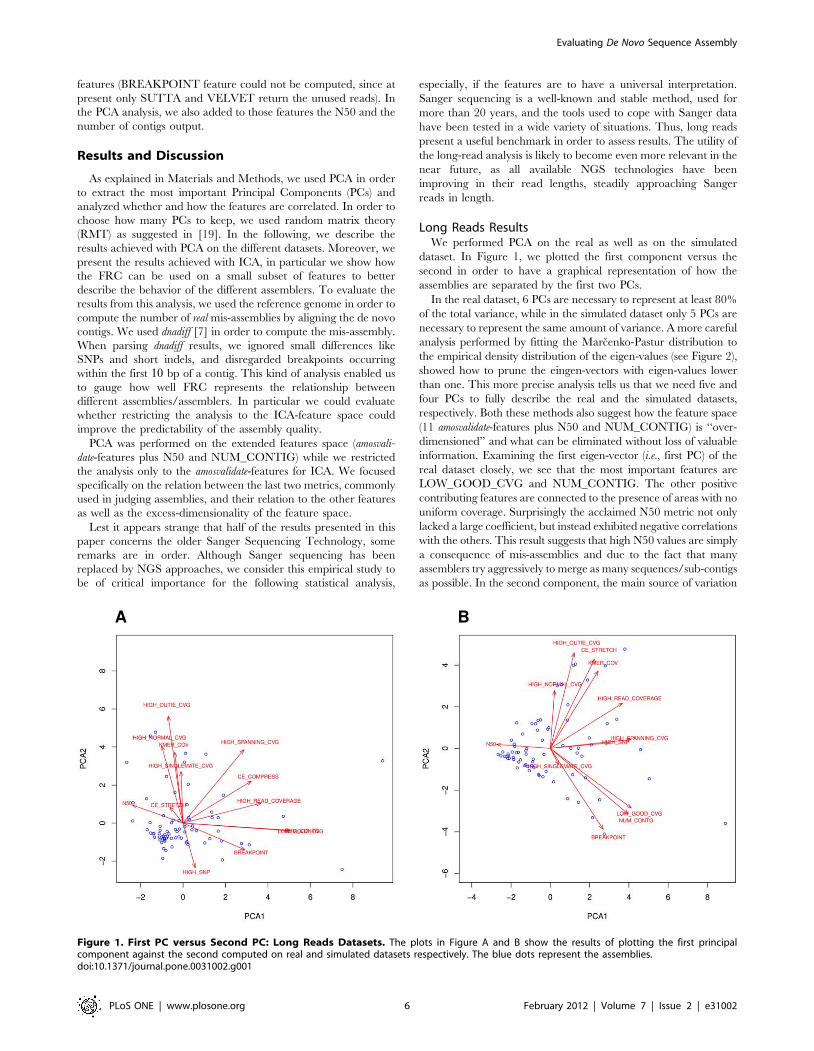
Long Reads ResultsWe performed PCA on the real as well as on the simulated

dataset. In Figure 1, we plotted the first component versus the

second in order to have a graphical representation of how the

assemblies are separated by the first two PCs.

In the real dataset, 6 PCs are necessary to represent at least 80%

of the total variance, while in the simulated dataset only 5 PCs are

necessary to represent the same amount of variance. A more careful

analysis performed by fitting the Marcenko-Pastur distribution to

the empirical density distribution of the eigen-values (see Figure 2),

showed how to prune the eingen-vectors with eigen-values lower

than one. This more precise analysis tells us that we need five and

four PCs to fully describe the real and the simulated datasets,

respectively. Both these methods also suggest how the feature space

(11 amosvalidate-features plus N50 and NUM_CONTIG) is ‘‘over-

dimensioned’’ and what can be eliminated without loss of valuable

information. Examining the first eigen-vector (i.e., first PC) of the

real dataset closely, we see that the most important features are

LOW_GOOD_CVG and NUM_CONTIG. The other positive

contributing features are connected to the presence of areas with no

uniform coverage. Surprisingly the acclaimed N50 metric not only

lacked a large coefficient, but instead exhibited negative correlations

with the others. This result suggests that high N50 values are simply

a consequence of mis-assemblies and due to the fact that many

assemblers try aggressively to merge as many sequences/sub-contigs

as possible. In the second component, the main source of variation

Figure 1. First PC versus Second PC: Long Reads Datasets. The plots in Figure A and B show the results of plotting the first principalcomponent against the second computed on real and simulated datasets respectively. The blue dots represent the assemblies.doi:10.1371/journal.pone.0031002.g001



among assemblies with a large number of features is due to mis-

assembled repeats (HIGH_READ_COVERAGE, K_MER_COV,

HIGH_OUTIE_CVG, and HIGH_SPANNING_CVG), a low

number of contigs and SNPs. The first three components account

for the 55% of the total variation.

Examining the results from the simulated datasets, we noticed

that no COMPRESSION feature has been found in any of the

assemblies. The first eigen vector of the simulated dataset is similar

to the ones obtained from real data, indicating a consistency

between the two analyses. Again LOW_GOOD_CVG and

NUM_CONTIG are among the most important features and

N50 is again negatively correlated. The second component is

similar to the one obtained from real data, as the main source of

variation is again between assemblies characterized by repeats

assembled in the wrong copy number and assemblies with too few

contigs and breakpoints. The first three components account for

70% of the total variance.

A closer examination reveals that real and simulated PCs are

somewhat different. Despite a complete absence of a feature in the

simulated dataset (probably a failure of the read simulator to

properly simulate the insert variation), we notice several

differences: the first ‘‘simulated PC’’ gives non-negligible impor-

tance to features like STRETCH, HIGH_SNP, and KMER_

COV that have much smaller importance in the first ‘‘real PC.’’ A

similar situation holds true also for the second PC. The third

components are utterly different (see Table 1), but not unexpected.

We are thus led to conclude that sequence assembly evaluation

based on simulated experiments could be misleading, unless

genome sequence simulators are further improved.

The principal component analysis (PCA) convinced us that the

feature-space is highly over-dimensioned. Therefore we tried to

select from the feature space the more informative features in order

to estimate the performance of different assemblers on a small

feature subspace. This analysis, leading to feature selection, was

accomplished using another multivariate technique known as

Independent Component Analysis (ICA). Following the method

proposed in [22], we performed ICA using the fastICA algorithm

on the amosvalidate features. We extracted the Independent

Components (ICs) and selected the most representative feature

in each of the ICs with the highest kurtosis value. From the real

dataset, we selected the following 6 features: COMPRESSION,

HIGH_OUTIE_CVG, HIGH_SINGLEMATE_CVG, HIGH_

READ_COVERAGE, KMER_COV, and LOW_GOOD_CVG.

Figure 2. Marcenko-Pastur Distribution: Long Reads Datasets. We found the Marcenko-Pastur that best fits the eigen-value distribution. Alleigen-vectors with eigen-values under the Marcenko-Pastur function are considered non informative. Figure A shows the results obtained on reallong read, conversely Figure B shows the results obtained on simulated long reads.doi:10.1371/journal.pone.0031002.g002

Table 1. More Informative Principal Components For LongReads.

Real Simulated

FEATURES PC1 PC2 PC3 PC1 PC2 PC3

BREAKPOINT 0.29 20.14 20.21 0.26 20.38 20.04

COMPRESSION 0.32 0.22 0.35 - - -

STRETCH 20.06 0.08 0.27 0.22 0.42 0.12

HIGH_NORMAL_CVG 20.10 0.40 0.21 0.02 0.2 20.44

HIGH_OUTIE_CVG 20.07 0.56 20.09 0.12 0.46 0.01

HIGH_READ_COVERAGE 0.36 0.10 20.13 0.36 0.21 20.19

HIGH_SINGLEMATE_CVG 20.01 0.27 20.53 0.04 20.07 20.76

HIGH_SNP 0.05 20.23 20.13 0.30 0.02 20.18

HIGH_SPANNING_CVG 0.28 0.38 0.31 0.41 0.04 0.00

KMER_COV 20.03 0.37 20.48 0.24 0.37 0.16

LOW_GOOD_CVG 0.50 20.04 20.02 0.41 20.28 0.04

N50 20.23 0.09 0.20 20.27 0.01 20.30

NUM_CONTG 0.50 20.03 20.02 0.39 20.31 0.02

cumulative variation 27% 44% 55% 36% 59% 70%

First three PCs for the two long reads datasets: real long reads, simulated longreads. At the bottom of each component we reported the cumulative variationrepresented.doi:10.1371/journal.pone.0031002.t001



In Figure 3, we illustrate how the ICA-subspace allows better

evaluation of different assemblers. Figure 3 shows the FRC for the

assembly of the Brucella suis dataset computed on all the feature

space (Fig. 3A) and on the ICA-feature space (Fig. 3B). In the first

case, we see how, rather surprisingly, TIGR now behaves much

worse than all other assemblers, while PCAP, MINIMUS,

CABOG and SUTTA have comparable performances. It is

surprising that TIGR performs worse than MINIMUS, which

does not use the important information, available in paired reads.

Inspecting these two assemblies closely (Table 2), we see how

MINIMUS produces a highly fragmented assembly (206 contigs)

in comparison to TIGR (69 contigs). If we plot the FRC after

reducing the space to the only ICA-features (Fig. 3B) we obtain a

slightly different picture. Looking only at the most informative

features we discovered that CABOG performs better than all the

other assemblers, while SUTTA, TIGR and PCAP are more or

less equivalent. This picture is concordant with the results showed

in Table 2, from which we clearly see that MINIMUS is the

assembler with the poorest performance.

Last four columns of Table 2 show how, in general, by reducing

the feature space we are able to discard a large number of features

(in the TIGR case we pass from 1281 to 134 features) without

discarding any significant number of valid features (i.e., features

that coincide with real mis-assemblies). This statistics on true

discovery suggest that our method does not suffer from a lack of

desirable sensitivity. It was noticed in [7] that assembly features

have, in general, high sensitivity (higher than 98%) but they lack

specificity. We also noticed that the situation remains true even

after dimensionality reduction of the feature space. In general this

is a consequence of how features arise in two scenarios: features

that affect large portions of contigs and assembler-specific features.

In the first scenario a feature affects a large portion of a contig

when, however, only a relatively small fragment of such contig is a

true mis-assembly. The second scenario is much more problem-

atic, we noticed that some assemblers have a particular feature

that appears almost in every contig (in the case of Brucella suis,

LOW_GOOD_CVG appears in almost all TIGR contigs). When

this feature is selected by the ICA analysis the specificity is deeply

affected (however, the sensitivity remains high). This situation can

be avoided by selecting the most representative features for each

assembler, but a larger dataset of genomes is necessary in order to

successfully apply PCA and ICA.

Short Reads ResultsAs explained in the Materials and Methods Section, the real

short read dataset is somewhat different from the simulated ones.

In the real dataset, we used only four different genomes, sequenced

with Illumina producing reads of different lengths. In order to

obtain sufficiently many assemblies that could allow PCA and ICA

to be performed, we extracted and assembled subsets of reads with

different coverages. We selected four different kinds of reads, from

which it is possible to obtain as general a set of PCs as possible.

However it would have been preferable to obtain an even larger

and more representative datasets that could have led to more

accurate results. On the other hand, the simulated dataset was

obtained by simulating genomes of 20 different organisms at a

Figure 3. Feature Response Curve and ICA features: Long Reads. Figure A shows the FRC for the 5 assemblers on Brucella suis dataset whenusing all the feature space. Figure B shows the FRC computed on the ICA-selected features.doi:10.1371/journal.pone.0031002.g003

Table 2. Assembly Comparison Real Long Reads: Brucella suis.

Assembler # Ctg N50 (Kbp) Max (Kbp) Errs # Feat # corr Feat # ICA Feat # corr ICA Feat

CABOG 41 265 711 24 375 24 45 18

MINIMUS 205 31 89 44 382 37 208 36

PCAP 91 69 194 50 455 57 94 41

SUTTA 72 93 621 45 261 23 75 22

TIGR 69 111 357 31 1281 24 134 20

Brucella suis assemblies obtained with long reads have been compared using standard assembly statistics. We reported the assembler employed, the number of contigsreturned by the assembler, the N50 length, the length of the longest contig and the number of mis-assemblies identified by dnadiff. Moreover we reported the numberof features returned by amosvalidate and the number of such features that overlap with a real mis-assembly. The same data is reported for the ICA-features.doi:10.1371/journal.pone.0031002.t002



constant coverage (80|), comprising paired reads of length

100 bp and insert size of 600 bp. The results obtained using this

dataset gave us a picture of the state-of-the-art assembly

capabilities. However, as seen in the analyses of long reads, PCs

obtained through simulated data appear dissimilar to the real ones.

Again, PCA analysis on the real and simulated dataset (Table 3)

suggested the presence of highly ‘‘over-dimensioned’’ feature

space. While, to achieve just 80% of the variance, we need only 5

components in the real datasets, as few as 4 are adequate in the

simulated ones. Using more sophisticated random matrix theory

and the Marcenko-Pastur function, we observed that it is safe to

disregard an extra PC with no loss of accuracy in either of the

cases.

As far as the first real PC is concerned, we saw how the

LOW_GOOD_CVG and N50 are among the most important

features. Again, as in the long reads datasets, the two features are

negatively correlated. While in the first long read PC most of the

features were positively correlated, in the short read case it was no

longer true. We saw that compression and extension events

(COMPRESSION, STRETCH) are correlated to mate-pairs

problems (HIGH_OUTIE_CVG) while the number of contigs is

positively correlated to areas with low coverage. These effects can

be explained in the following way: areas with compression and

extension events are likely to contain a large number of mis-

oriented reads, while the production of an excess contigs can be a

consequence of a failure in properly estimating the copy number of

repeated sequences (thus resulting in a low coverage). The second

PC distinguishes assemblies with high HIGH_NORMAL_CVG.

All the other relevant features are negatively correlated to this one.

As expected, the PCs resulting from the simulated dataset

differed to some degree from the ones obtained from real datasets.

Also in this case N50 is negatively correlated and its coefficient is

not among the maximal ones (like in the long read case). The first

component is similar to the first component of the simulated long

read dataset. In the second component the main source of

variation between assemblies could be explained by a low number

of contigs and regions covered only by unpaired reads as well as a

large number of compression expansion events and mate pairs in

different contigs.

Using ICA we extracted two feature subsets: one for the real data

and the other for the simulated data. As before, we considered ICs

that account for 80% of the kurtosis distribution. The ICA-space for

the real dataset is formed by 6 features: COMPRESSION,

LOW_GOOD_CVG, KMER_COV, HIGH_SPANNING_CVG,

HIGH_OUTIE_CVG, and CE_STRETCH.

In Figure 4 we draw the FRC for the E. coli dataset composed of

paired reads of length 36 bp that form a 130| coverage of the

sequenced genome. Figure 4A represents the FRC computed on

all the feature space, while Figure 4B represents the FRC

computed on the ICA-space. When all features are employed

(Fig. 4A), we can clearly see how SUTTA, ABySS and SOAP

outperform RAY and VELVET. This situation is in contrast with

the analysis presented in Table 4, where we clearly see that RAY is

the assembler generating very few mis-assemblies along with

ABySS, SUTTA and SOAP all behaving similarly. VELVET has

Table 3. More Informative Principal Components For ShortReads.

Real Simulated

FEATURES PC1 PC2 PC3 PC1 PC2 PC3

BREAKPOINT - - - - - -

COMPRESSION 20.28 20.15 0.24 0.32 0.20 0.33

STRETCH 20.30 20.11 0.32 0.2 0.37 0.26

HIGH_NORMAL_CVG 0.12 0.44 20.09 0.15 0.13 20.62

HIGH_OUTIE_CVG 20.32 20.33 20.29 0.19 0.15 20.536

HIGH_READ_COVERAGE 20.26 20.30 20.41 0.35 0.09 20.01

HIGH_SINGLEMATE_CVG 0.23 20.26 20.37 20.11 20.50 0.15

HIGH_SNP 20.19 20.05 20.38 0.37 0.00 20.06

HIGH_SPANNING_CVG 20.07 20.38 0.12 0.36 20.24 20.16

KMER_COV 20.08 20.22 0.47 0.31 0.28 0.28

LOW_GOOD_CVG 0.41 20.32 0.09 0.34 20.35 0.09

N50 20.48 0.08 0.10 20.19 0.25 0.02

NUM_CONTG 0.36 20.41 0.12 0.30 20.42 0.03

cumulative variation 26% 50% 63% 43% 62% 75%

First three PCs for the two short reads datasets: real short reads and, simulatedshort reads. At the bottom of each component we reported the cumulativevariation represented.doi:10.1371/journal.pone.0031002.t003

Figure 4. Feature Response Curve and ICA features: Real Short Reads. Figure A shows the FRC for the 5 assemblers on E. coli real dataset(read length 36 bp, insert size 200 bp and coverage 130|) when using all the feature space. Figure B shows the FRC computed on the ICA-selectedfeatures.doi:10.1371/journal.pone.0031002.g004



much larger number of mis-assemblies, suggesting that the long

contigs that it produces are often a consequence of incorrect

choices. If we reduce to the ICA-subspace (Fig. 4B) the picture

changes drastically but some problems still remain: RAY, as one

would expect, becomes the best assembler, but it is now

surprisingly closely followed by VELVET. Moreover, ABySS

becomes one of the worst assemblers. This situation is probably a

consequence of the way in which features have been computed:

ABySS and SOAP provide no facility but to map reads back to the

contigs in order to build a layout (it is not clear if the other De-

Bruijn based assemblers build a real Sanger-like layout or if they

make use of heuristics). This indirect approach clearly skews our

empirical analysis. Nonetheless, we can see how the reduced ICA

space is able to highlight the good performances of RAY. The last

four columns of Table 4 show that ICA-features significantly

reduce the number of features to be considered (even if this time

the reduction is not as impressive as the one obtained with long

reads) without noticeably affecting the number of real features

(with the only exception of VELVET). This picture again

motivates us to highlight the need for assemblers to provide read

layouts that could ensure a meaningful evaluation.

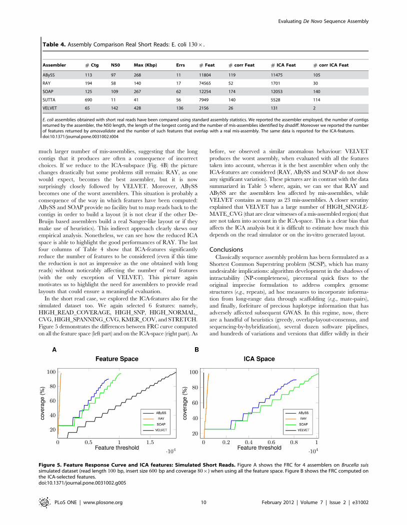
In the short read case, we explored the ICA-features also for the

simulated dataset too. We again selected 6 features: namely,

HIGH_READ_COVERAGE, HIGH_SNP, HIGH_NORMAL_

CVG, HIGH_SPANNING_CVG, KMER_COV, and STRETCH.

Figure 5 demonstrates the differences between FRC curve computed

on all the feature space (left part) and on the ICA-space (right part). As

before, we observed a similar anomalous behaviour: VELVET

produces the worst assembly, when evaluated with all the features

taken into account, whereas it is the best assembler when only the

ICA-features are considered (RAY, ABySS and SOAP do not show

any significant variation). These pictures are in contrast with the data

summarized in Table 5 where, again, we can see that RAY and

ABySS are the assemblers less affected by mis-assemblies, while

VELVET contains as many as 23 mis-assemblies. A closer scrutiny

explained that VELVET has a large number of HIGH_SINGLE-

MATE_CVG (that are clear witnesses of a mis-assembled region) that

are not taken into account in the ICA-space. This is a clear bias that

affects the ICA analysis but it is difficult to estimate how much this

depends on the read simulator or on the in-vitro generated layout.

ConclusionsClassically sequence assembly problem has been formulated as a

Shortest Common Superstring problem (SCSP), which has many

undesirable implications: algorithm development in the shadows of

intractability (NP-completeness), piecemeal quick fixes to the

original imprecise formulation to address complex genome

structures (e.g., repeats), ad hoc measures to incorporate informa-

tion from long-range data through scaffolding (e.g., mate-pairs),

and finally, forfeiture of precious haplotype information that has

adversely affected subsequent GWAS. In this regime, now, there

are a handful of heuristics (greedy, overlap-layout-consensus, and

sequencing-by-hybridization), several dozen software pipelines,

and hundreds of variations and versions that differ wildly in their

Table 4. Assembly Comparison Real Short Reads: E. coli 130|.

Assembler # Ctg N50 Max (Kbp) Errs # Feat # corr Feat # ICA Feat # corr ICA Feat

ABySS 113 97 268 11 11804 119 11475 105

RAY 194 58 140 17 74565 52 1701 30

SOAP 125 109 267 62 12254 174 12053 140

SUTTA 690 11 41 56 7949 140 5528 114

VELVET 65 142 428 136 2156 26 131 2

E. coli assemblies obtained with short real reads have been compared using standard assembly statistics. We reported the assembler employed, the number of contigsreturned by the assembler, the N50 length, the length of the longest contig and the number of mis-assemblies identified by dnadiff. Moreover we reported the numberof features returned by amosvalidate and the number of such features that overlap with a real mis-assembly. The same data is reported for the ICA-features.doi:10.1371/journal.pone.0031002.t004

Figure 5. Feature Response Curve and ICA features: Simulated Short Reads. Figure A shows the FRC for 4 assemblers on Brucella suissimulated dataset (read length 100 bp, insert size 600 bp and coverage 80|) when using all the feature space. Figure B shows the FRC computed onthe ICA-selected features.doi:10.1371/journal.pone.0031002.g005



preprocessing, parameters, and post-hoc analysis. Yet, accuracy

and suitability of assemblies produced by any of these systems have

remained largely unexamined. Attempts have been made to

validate the results of an assembler either with simulated in silico

data or with auxiliary information from genetic or physical maps,

or by sequencing randomly selected short fragments. These

approaches have not succeeded – either hampered by the

inaccuracy of the tests themselves, or by the additional cost-

overhead they could incur.

A different approach has now emerged from attempts to

validate the assemblies by examining various features of read lay-

outs, which could be indicative of sources of misassemblies. These

features have also led to a new technique for assembly comparison

using Feature-Response Curves (FRC). However, in the absence of

a thorough and rigorous analysis of the structure of the feature-

space, FRC analysis lacked a solid foundational grounding. This

paper addresses these issues via principal and independent

component analyses (PCA and ICA, respectively) that identify

key features and how each of them is related to the other features.

The paper cocluded that most features are redundant, few of the

widely accepted features are not very good predictors of accuracy,

and a small number of good features can be isolated relatively

easily without affecting the methods sensitivity. These analyses

have quantified our insight into why none of the existing

assemblers has been satisfactory.

But further work needs to be done. Reducing the Feature-space

through Independent Component Analysis does not solve the lack of

specificity of the method. It is not clear if this is a consequence of the

currently designed features and if new features can circumvent this

problem. We identified as a major stumbling block in obtaining

reliable results, the lack of NGS-based assemblers producing an

assembly-layout. There are some fundamental (but unavoidable)

biases in our techniques. For instance, how robust is our detected

redundancy in the current set of features? A premature elimination of

a feature, presumed redundant, could be imprudent, especially if it is

later determined that the detected redundancy depended on the

currently existing set of assembly algorithms that created the

examples for the supervised learning. We have tried to avoid possible

biases by selecting representative sets of algorithms from all three

known paradigms: SBH (sequencing-by-hybridization), OLC (over-

lap-layout-consensus) and B&B (branch-and-bound). Currently, the

only example from B&B (e.g., exhaustive global optimization) is

SUTTA (with some variations: aggressive vs. conservative), although,

for the other classes, there are many more. In the near future, we

expect to see more SUTTA-like algorithms (or even innovation of

new assembly paradigms), which will require continual updating of

the results reported here. In contrast, the idea of distilling an unbiased

set of features of existing genomes (not algorithms) is likely to be less

variable, since the samples of genomes used already contain a wide

variety of structural elements. The set of features extracted in this way

could lead to more realistic in silico genome models, which in turn can

be used in training and assessing assembly algorithms – e.g.,

identifying a set of features for existing genomes that expose classes

of errors or inconsistencies, intrinsic to a specific assembler.

In the future, we expect to see more analysis of this nature, not

just to understand the feature-space and its redundancy, but also

to understand how newer algorithms, technologies (e.g., next-next-

generation sequencing, long-range mapping – including dilution,

mate pairs, strobe reads, optical mapping, etc.), and testing

strategies (based on simulation or better references) will affect

not only the way old (negative) features are tamed and new

features are invented, but also the redundancy structure of the

feature-space itself. Related to these issues, there is also the

question of how a subset of informative features can be learned, so

that a global optimization formulation of the sequence assembly

problem (in terms of few score and penalty functions involving

these features) would lead to higher fidelity. Recently developed

SUTTA assembly algorithm, based on branch-and-bound, is

specifically designed to exploit such global formulations. There are

also many thorny issues related to how to develop better in silico

genome sequence simulation, benchmark datasets, data standards,

and a trusted institution with the authority to validate genome

assemblies.

Supporting Information

Document S1 Complete experiments description. This

document contains a detailed list of genomes used in the paper and

the commands used to obtain the simulated data.

(PDF)

Acknowledgments

We would like to thank Prof. A. Policriti of University of Udine and

‘‘Istituto di Genomica Applicat’’ (IGA), Fabian Menges of NYU as well as

NYU Bioinformatics Group and IGA’s staff, for providing advice and

support. We would also like to thank several of our colleagues for insightful

comments on an early draft of the paper: Profs. G. Atwal, M. Schatz and

M. Wigler of Cold Spring Harbor Lab, Prof. R. Rabadan of Columbia

University, Prof. M. Pop of University of Maryland, Dr. A. Phillippy of

National Biodefense Analysis and Countermeasure Center (NBACC), Dr.

C. Cantor of Sequenom and Dr. T.S. Anantharaman of BioNanoGe-

nomics, LLC. We also wish to thank an anonymous reviewer, whose

comments led to a much clearer discussion of the possible biases in our

feature-learning algorithms, along with several possible remedies.

Author Contributions

Conceived and designed the experiments: FV GN BM. Performed the

experiments: FV. Analyzed the data: FV GN BM. Contributed reagents/

materials/analysis tools: FV GN. Wrote the paper: FV GN BM.

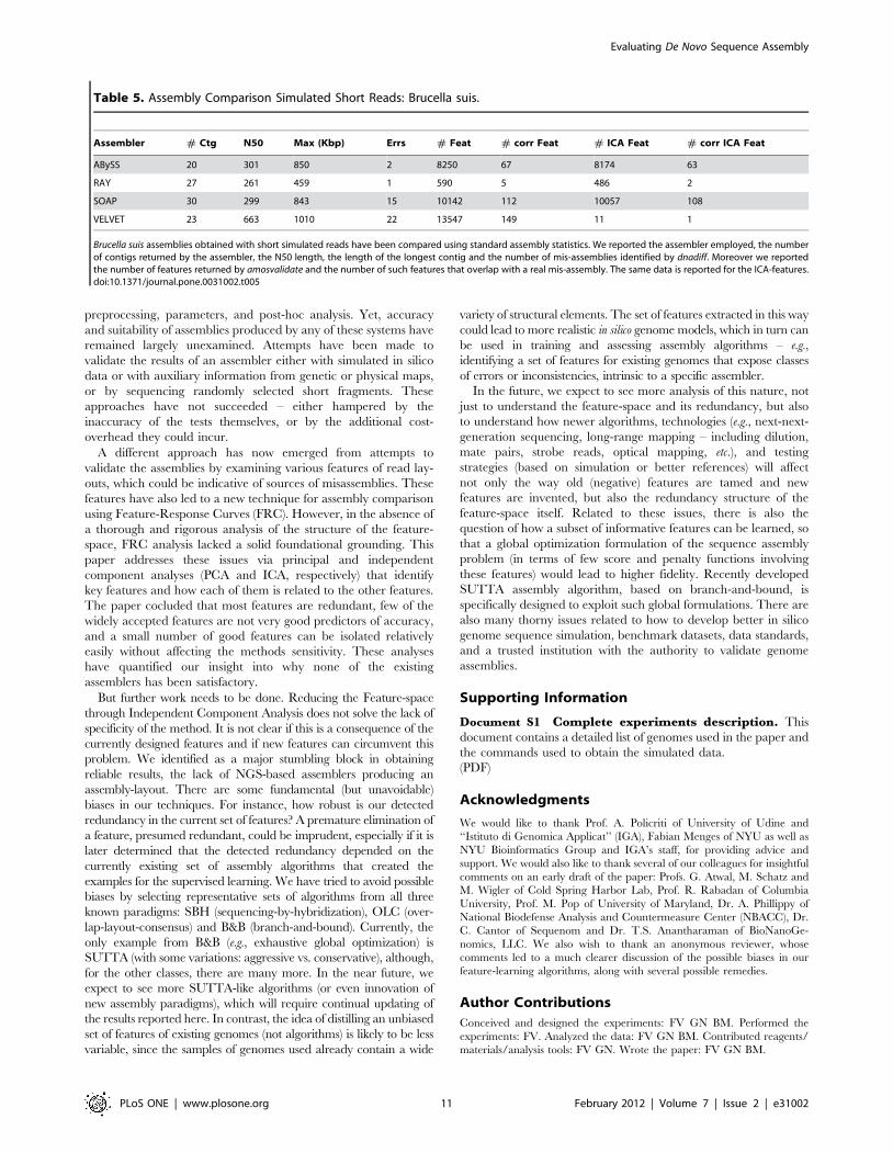
Table 5. Assembly Comparison Simulated Short Reads: Brucella suis.

Assembler # Ctg N50 Max (Kbp) Errs # Feat # corr Feat # ICA Feat # corr ICA Feat

ABySS 20 301 850 2 8250 67 8174 63

RAY 27 261 459 1 590 5 486 2

SOAP 30 299 843 15 10142 112 10057 108

VELVET 23 663 1010 22 13547 149 11 1

Brucella suis assemblies obtained with short simulated reads have been compared using standard assembly statistics. We reported the assembler employed, the numberof contigs returned by the assembler, the N50 length, the length of the longest contig and the number of mis-assemblies identified by dnadiff. Moreover we reportedthe number of features returned by amosvalidate and the number of such features that overlap with a real mis-assembly. The same data is reported for the ICA-features.doi:10.1371/journal.pone.0031002.t005



References

1. Narzisi G, Mishra B (2010) Scoring-and-Unfolding Trimmed Tree Assembler:Concepts, Constructs and Comparisons. Bioinformatics (Oxford, England) 27:

153–160.2. Menges F, Narzisi G, Mishra B (2011) TOTALRECALLER : Improved

Accuracy and Performance via Integrated Alignment & Base-Calling. Bioinfor-matics (Oxford, England). pp 1–8.

3. Li R, Fan W, Tian G, Zhu H, He L, et al. (2009) The sequence and de novo

assembly of the giant panda genome. Nature 463: 311–317.4. Nagarajan N, Pop M (2009) Parametric complexity of sequence assembly:

Theory and applications to next generation sequencing. Journal of Computa-tional Biology 16: 897–908.

5. Lander ES, Linton LM, Birren B, Nusbaum C, Zody MC, et al. (2001) Initial

sequencing and analysis of the human genome. Nature 409: 860–921.6. Lin Y, Li J, Shen H, Zhang L, Papasian C, et al. (2011) Comparative Studies of

de novo Assembly Tools for Next-generation Sequencing Technologies.Bioinformatics. pp 1–7.

7. Phillippy AM, Schatz MC, Pop M (2008) Genome assembly forensics: finding

the elusive misassembly. Genome biology 9: R55.8. Narzisi G, Mishra B (2011) Comparing De Novo Genome Assembly: The Long

and Short of It. PLoS ONE 6: e19175.9. Miller J, Koren S, Sutton G (2010) Assembly algorithms for next-generation

sequencing data. Genomics. pp 1–13.10. Earl DA, Bradnam K, St John J, Darling A, Lin D, et al. (2011) Assemblathon 1:

A competitive assessment of de novo short read assembly methods. Genome

Research.11. Salzberg SL, Phillippy AM, Zimin AV, Puiu D, Magoc T, et al. (2011) Gage: A

critical evaluation of genome assemblies and assembly algorithms. GenomeResearch.

12. Jolliffe I (2002) Principal Component Analysis, Second Edition. Wiley Online

Library.13. Hyvarinen A, Karhunen J, Erkki O (2001) Independent Component Analysis.

John Wiley & Sons, first edition.14. Lu H, Plataniotis K, Venetsanopoulos A (2011) A survey of multilinear subspace

learning for tensor data. Pattern Recognition 44: 1540–1551.15. Imam I, Vafaie H (1994) An empirical comparison between global and greedy-

like search for feature selection. In: Proceedings of the Florida AI Research

Symposium (FLAIRS-94), Pensacola Beach, FL Citeseer. pp 66–70.16. Bi J, Bennett K, Embrechts M, Breneman C, Song M (2003) Dimensionality

reduction via sparse support vector machines. The Journal of Machine LearningResearch 3: 1229–1243.

17. Boutsidis C, Mahoney M, Drineas P (2008) Unsupervised feature selection for

principal components analysis. In: Proceeding of the 14th ACM SIGKDD

international conference on Knowledge discovery and data mining ACM. pp

61–69.

18. Prasad M, Sowmya A, Koch I (2004) Efficient feature selection based on

independent component analysis. In: Intelligent Sensors, Sensor Networks and

Information Processing Conference, 2004. Proceedings of the 2004 IEEE. pp

427–432. doi:10.1109/ISSNIP.2004.1417499.

19. Johnstone I (2006) High dimensional statistical inference and random matrices.

Arxiv preprint math/0611589.

20. Hyvarinen A, Oja E (1997) A fast fixed-point algorithm for independent

component analysis. Neural computation 9: 1483–1492.

21. Liu J, Pearlson G, Windemuth A, Ruano G, Perrone-Bizzozero N, et al. (2009)

Combining fMRI and SNP data to investigate connections between brain

function and genetics using parallel ICA. Human brain mapping 30: 241–255.

22. Nahlawi LI, Mousavi P (2010) Single nucleotide polymorphism selection using

independent component analysis. Annual International Conference of the IEEE

Engineering in Medicine and Biology Society IEEE Engineering in Medicine

and Biology Society Conference 2010: 6186–9.

23. Miller JR, Delcher AL, Koren S, Venter E, Walenz BP, et al. (2008) Aggressive

assembly of pyrosequencing reads with mates. Bioinformatics (Oxford, England)

24: 2818–24.

24. Sommer DD, Delcher AL, Salzberg SL, Pop M (2007) Minimus: a fast,

lightweight genome assembler. BMC bioinformatics 8: 64.

25. Huang X, Yang SP (2005) Generating a genome assembly with PCAP. Current

protocols in bioinformatics/editoral board, Andreas D Baxevanis [et al] Chapter

11: Unit11.3.

26. Sutton G, White O, Adams M, Kerlavage A (1995) TIGR Assembler: A new

tool for assembling large shotgun sequencing projects. Genome Science and

Technology 1: 9–19.

27. Richter DC, Ott F, Auch AF, Schmid R, Huson DH (2008) MetaSim: a

sequencing simulator for genomics and metagenomics. PloS one 3: e3373.

28. Zerbino D, Birney E (2008) Velvet: algorithms for de novo short read assembly

using de Bruijn graphs. Genome research 18: 821–829.

29. Boisvert S, Laviolette F, Corbeil J (2010) Ray: Simultaneous Assembly of Reads

from a Mix of High-Throughput Sequencing Technologies. Journal of

Computational Biology 17: 101020044546029.

30. Simpson J, Wong K, Jackman S, Schein J (2009) ABySS: A parallel assembler for

short read sequence data. Genome. pp 1117–1123.

31. Li R, Zhu H, Ruan J, Qian W, Fang X, et al. (2010) De novo assembly of

human genomes with massively parallel short read sequencing. Genome

research 20: 265–72.



feature-by-feature – evaluating de novosequence …...feature-by-feature – evaluating de...

Documents