Purdue UniversityPurdue e-Pubs

Open Access Theses Theses and Dissertations

Spring 2014

Feasibility of Pulsed Proton Induced Acoustics for3D DosimetryFahed M. AlsaneaPurdue University

Follow this and additional works at: https://docs.lib.purdue.edu/open_access_theses

Part of the Biomedical Engineering and Bioengineering Commons, and the Oncology Commons

This document has been made available through Purdue e-Pubs, a service of the Purdue University Libraries. Please contact epubs@purdue.edu foradditional information.

Recommended CitationAlsanea, Fahed M., "Feasibility of Pulsed Proton Induced Acoustics for 3D Dosimetry" (2014). Open Access Theses. 147.https://docs.lib.purdue.edu/open_access_theses/147

01 14

PURDUE UNIVERSITY GRADUATE SCHOOL

Thesis/Dissertation Acceptance

Thesis/Dissertation Agreement.Publication Delay, and Certification/Disclaimer (Graduate School Form 32)adheres to the provisions of

Department

Fahed M. Alsanea

Feasibility of Pulsed Proton Induced Acoustics for 3D Dosimetry

Master of Science

KEITH STANTZ

SHUANG LIU

ULRIKE DYDAK

KEITH STANTZ

WEI ZHENG 04/18/2014

i

FEASIBILITY OF PULSED PROTON ACOUSTICS FOR 3D DOSIMETRY

A Thesis

Submitted to the Faculty

of

Purdue University

by

Fahed M Alsanea

In Partial Fulfillment of the

Requirements for the Degree

of

Master of Science

May 2014

Purdue University

West Lafayette, Indiana

ii

Dedicated to my mother

iii

ACKNOWLEDGEMENTS

This work was made possible by the support of my advisor Dr. Keith Stantz. His

patient guidance, useful critiques, and research abilities in this work were essential. I am

delighted to have worked with him on this novel concept in the medical physics field. I

would like to express my very great appreciation and gratitude toward Dr. Stantz.

My gratitude is extended to my committee members, Dr. Ulrike Dydak, and Dr.

Shaung Liu for their support. I would also like to acknowledge Dr. Vadim Moskvin for

his input in Monte Carlo Simulations. Special thanks go to Dr. Indra Das and Dr.

Klyachko (Sasha) from Indiana University School of Medicine. I would also like to thank

my fellow lab members: Akshay Prabhu Verleker, Alison Roth, Mark Krutulis, and Justin

Sick. Last but not least, I would like to thank my family for their daily support and

encouragements.

iv

TABLE OF CONTENTS

Page

LIST OF TABLES ............................................................................................................. vi LIST OF FIGURES .......................................................................................................... vii NOMENCLATURE ........................................................................................................... x

ABSTRACT ............................................................................................................. xii CHAPTER 1. INTRODUCTION ................................................................................. 1

1.1 Background and Innovation ...................................................................... 1

1.2 Radiation Acoustics Theory ...................................................................... 6

1.3 Imaging Techniques .................................................................................. 9

1.3.1 Computed Tomography .................................................................... 10

1.3.2 Delay and Sum ................................................................................. 12

CHAPTER 2. METHODOLOGY .............................................................................. 14

2.1 Simulations .............................................................................................. 14

2.2 Scanner Design ........................................................................................ 15

2.3 Monte Carlo Simulation .......................................................................... 16

2.4 Pressure Signal ........................................................................................ 17

2.5 Proton Beam Pulse Width and Shape ...................................................... 18

2.6 Ultrasound Transducers........................................................................... 19

CHAPTER 3. RESULTS ............................................................................................ 21

3.1 Pressure Signal ........................................................................................ 21

3.2 RACT Signal Compared to Monte Carlo Dose ....................................... 24

3.3 Transducer Results .................................................................................. 29

CHAPTER 4. CONCLUSION, DISCUSSION AND FUTURE AIM ....................... 34

4.1 Feasibility ................................................................................................ 34

4.2 IU Blomington Proton Facility Experiment ............................................ 36

4.2.1 Methods ............................................................................................ 37

4.2.2 Results and Conclusion .................................................................... 42

v

Page

4.3 Proton Facilities....................................................................................... 45

4.4 Conclusion ............................................................................................... 45

LIST OF REFERENCES .................................................................................................. 46

vi

LIST OF TABLES

Table .............................................................................................................................. Page

Table 3.1 The results of the signal recording using a 500kHz center frequency

transducer. ........................................................................................................ 31

Table 3.2 The results of using a pre-amplifier with 54 dB gain. ...................................... 32

vii

LIST OF FIGURES

Figure ............................................................................................................................. Page

Figure 1.1 Thermoacoustic mechanism .............................................................................. 6

Figure 1.2 demonstrates the change in energy absorption. ................................................. 8

Figure 1.3 Parameters in the Gruneiesen Coefficient ......................................................... 9

Figure 1.4 Delay and Sum schematic ............................................................................... 13

Figure 1.5 The reconstruction of a point source located at 74 mm away from the

transducer ...................................................................................................... 13

Figure 2.1 The geometry of the transducer array used to simulate the excess pressure

created from the dose deposited from a proton beam. .................................. 15

Figure 2.2 IU HPTC treatment nozzle model implemented on FLUKA CG geometry

package. ......................................................................................................... 17

Figure 2.3 The simulated pulsed proton beam defined by T(t), where the leading and

falling edge is approximated by a linear function which is the derivative at

the center of the integrated Gaussian. ........................................................... 18

Figure 2.4 An impulse response (top) of 500kHz transducer with the frequency spectrum

(bottom). The Gaussian fit of the spectrum (red dashed line) produced a

center of 0.482 MHz and width of 0.226 MHz. ............................................ 19

Figure 3.1 Demonstrates the sensitivity of the radioacoustic CT scanner with regards to

the pulse width and rise time of the proton beam. ......................................... 22

viii

Figure ............................................................................................................................. Page

Figure 3.2 Demonstrating the excess pressure signal for three different beam parameters

with a transducer (PW, RT, and Beam width), using a transducer with

(S=40dB; SNR=40dB; preamp=40dB). ........................................................ 23

Figure 3.3 Simulated Pressure signal for a Pulsed Proton beam with Pulse width of 1

micorsecond and Rise time of 0.1 microsecond. ........................................... 24

Figure 3.4 Displayed is the MC simulated dose (per proton) on a voxel-wise basis for a

pencil proton beam with a range of 27cm in Water (left) and the

reconstructed image from the radiation acoustic computed tomographic

filtered backprojection algorithm (right), based on simulated thermoacoustic

pressure signal. .............................................................................................. 25

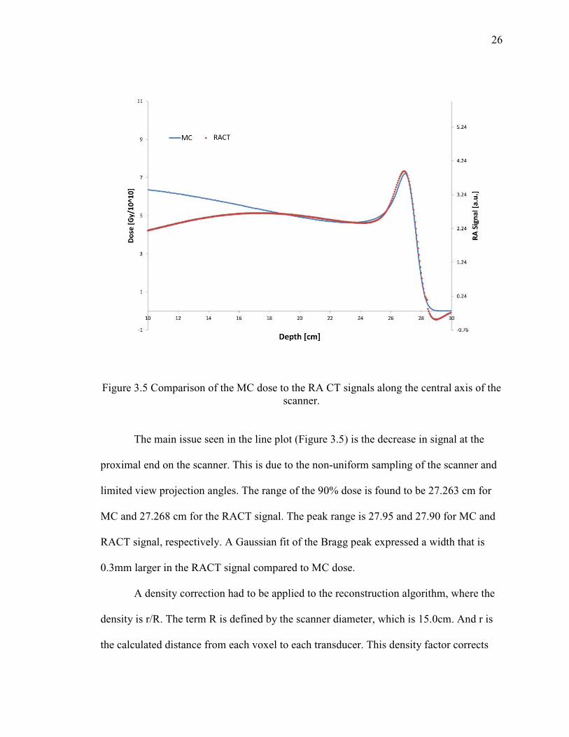
Figure 3.5 Comparison of the MC dose to the RA CT signals along the central axis of the

scanner. .......................................................................................................... 26

Figure 3.6 Three center profiles demonstrating the density correction applied (bottom). 27

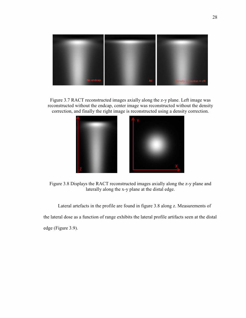
Figure 3.7 RACT reconstructed images axially along the z-y plane. Left image was

reconstructed without the endcap, center image was reconstructed without the

density correction, and finally the right image is reconstructed using a density

correction. ...................................................................................................... 28

Figure 3.8 Displays the RACT reconstructed images axially along the z-y plane and

laterally along the x-y plane at the distal edge. ............................................. 28

Figure 3.9 Beam width as a function of range for Monte Carlo simulation and the RACT

signals for Proton Beam with 27cm Range. .................................................. 29

ix

Figure ............................................................................................................................. Page

Figure 3.10 The Frequency components of the acoustic signal shown in Figure 3.3,

superimposed with the transducer spectrum (blue). ...................................... 30

Figure 3.11 Laser Calibration Data ................................................................................... 31

Figure 3.12 Signals recorded using the pulsed laser source with increasing output......... 32

Figure 3.13 Using a pre-amp with 54 dB gain the same signal shows an increase in

intensity. ........................................................................................................ 33

Figure 4.1 Water Tank Phantom to position and translate the ultrasound transducer. ..... 38

Figure 4.2 The experiment modification using a lead sheet. ............................................ 40

Figure 4.3 Tektronix OpenChoice Desktop Software is used to send settings and acquire

data. ............................................................................................................... 41

Figure 4.4 An ultrasound signal recorded using the oscilloscope and triggered using the

laser. Approximate position of the transducer was 15 mm. .......................... 41

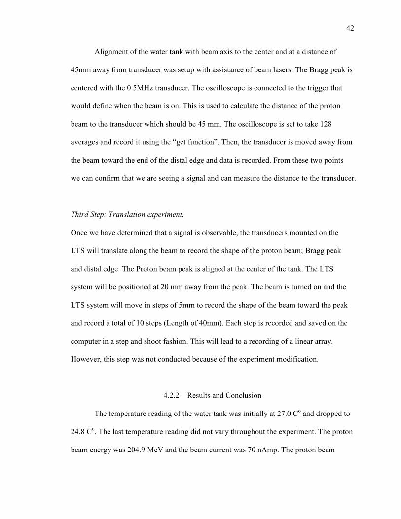
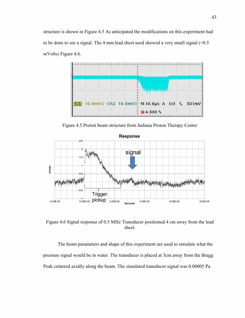
Figure 4.5 Proton beam structure from Indiana Proton Therapy Center .......................... 43

Figure 4.6 Signal response of 0.5 MHz Transducer positioned 4 cm away from the lead

sheet. .............................................................................................................. 43

Figure 4.7 Simulation of Bloomington Experiment using the Water Phantom. The Blue

line is the simulated pressure signal and the red line is the transducer signal

(500kHz, 50% Bandwidth). ........................................................................... 44

x

NOMENCLATURE

RACT Radioacoustic Computed Tomography

MC Monte Carlo

PET Positron Emission Tomography

PG Promt Gamma

CT Computed Tomography

RA Radiation Acoustics

3D Three Dimensional

2D Two Dimensional

qext Rate of Heating

β Thermal Volume Expansion

c Heat Capacity

Kt Thermal Compressibility

ρ Density

vs Velocity of Sound

Γ Gruiniesen Coefficient

T(r,t) Temperature Function

P(r,t) Pressure Signal

H(w) Filter Function

xi

A(w) Apodizing Function

I(w) Impulse Response

tPW Pulse Width

∆t Rise Time

λ Projection

IFT Inverse Fourier Transform

FWHM Full Width Half Max

LTS Linear Translation System

RMS Root Mean Square

SNR Signal to Noise Ratio

xii

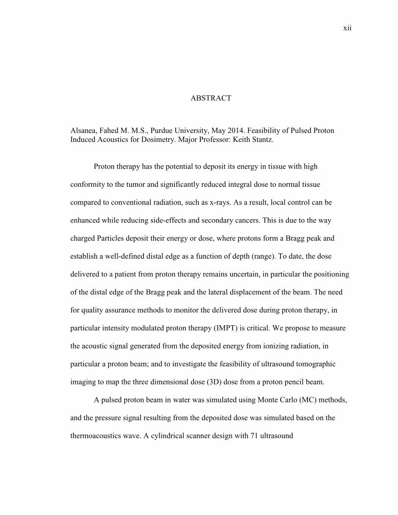
ABSTRACT

Alsanea, Fahed M. M.S., Purdue University, May 2014. Feasibility of Pulsed Proton Induced Acoustics for Dosimetry. Major Professor: Keith Stantz.

Proton therapy has the potential to deposit its energy in tissue with high

conformity to the tumor and significantly reduced integral dose to normal tissue

compared to conventional radiation, such as x-rays. As a result, local control can be

enhanced while reducing side-effects and secondary cancers. This is due to the way

charged Particles deposit their energy or dose, where protons form a Bragg peak and

establish a well-defined distal edge as a function of depth (range). To date, the dose

delivered to a patient from proton therapy remains uncertain, in particular the positioning

of the distal edge of the Bragg peak and the lateral displacement of the beam. The need

for quality assurance methods to monitor the delivered dose during proton therapy, in

particular intensity modulated proton therapy (IMPT) is critical. We propose to measure

the acoustic signal generated from the deposited energy from ionizing radiation, in

particular a proton beam; and to investigate the feasibility of ultrasound tomographic

imaging to map the three dimensional dose (3D) dose from a proton pencil beam.

A pulsed proton beam in water was simulated using Monte Carlo (MC) methods,

and the pressure signal resulting from the deposited dose was simulated based on the

thermoacoustics wave. A cylindrical scanner design with 71 ultrasound

xiii

transducers focused to a centeral point within the scanner was utilized. Finally, a 3-D

filtered backprojection algorithm was developed to reconstruct computed tomographic

images of the deposited dose. The MC dose profile was compared to the radioacoustic

reconstructed images, and the dependency of the proton pulse sequence parameters, pulse

width (tPW) and rise time (∆t), on sensitivity were investigated.

Based on simulated data, the reconstructed radioacoustic image intensity was

within 2%, on average, of the MC generated dose within the Bragg peak, and the location

of the distal edge was within 0.5mm. The simulated pressure signal for different tPW and

∆t for the same number of protons (1.8x107) demonstrated that compressing the protons

in a shorter period of time significantly increased the thermoacoustic signal and thus

sensitivity.

This study demonstrates that computed tomographic scanner based on ionizing

radiation induced acoustics can be used to verify dose distribution and proton range.

Realizing this technology into the clinic will have significant impact on treatment

verification during particle beam therapy and image guided techniques.

1

CHAPTER 1. INTRODUCTION

1.1 Background and Innovation

Over the past century, the use of radiation has been used to target and treat cancer,

where as of today, nearly half of all patients are treated with ionizing radiation. Critical to

the use of ionizing radiation is the accuracy and precision at which it is applied, where

advances in radiation physics and radiology, or imaging technology, has provide major

advances in x-ray therapy, such as 3D conformal radiation therapy, intensity modulate

radiation therapy (IMRT), and stereotactic radiosurgery (SRS), and tomotherapy. As with

the adoption of these new methods, proton therapy provides superior dose conformity to

the tumor volume while significantly reducing the integral dose to the surrounding

healthy tissue.[1] This is because a large fraction of the proton energy is deposited at the

end of its track with a steep fall-off, the Bragg peak and the distal edge. Due to the

targeted nature of proton therapy, and the advent of intensity modulated proton therapy,

the side-effects from radiation therapy and the risk of secondary cancers are and can be

substantially reduced, by potentially a factor of 2-10.[2-8] To take full advantage of these

gains, the high level of uncertainty and potential misapplication of the Bragg peak and

distal edge due to imprecise determination of stopping powers, patient and anatomical

positioning must be understood and overcome.

2

To date, the dose delivered to a patient from proton therapy remains uncertain, in

particular the positioning of the distal edge and lateral displacement of the beam. The

current trend in developing treatment quality assurance methods to monitor the results of

the delivery are the positron emission tomography method (PET) based on the detection

of the gamma quanta from the positron annihilation after decay of product from proton

induced nuclear reactions with oxygen and carbon in human tissue and the detection of

the prompt gamma (PG) accompanied the interaction of the protons with the tissue.

[9,10,11] The implementation of PET imaging for proton dosimtery and range

verification was first introduced by Maccabee et al. [12] Proton inelastic collisions form

the positron emitters 11C, 14N, and 15O, which upon annihilation emit two 0.511 MeV

photons. The dominant contribution to PET dosimetry is 15O; however, because of its

short half-life (2.037 min), 11C is the next dominant nuclide to measure. In addition to

their low overall production rate, radio-isotope production begins to fall off 2-3 cm prior

to the distal edge. To compensate, the data are convolved with the treatment plan using

filter functions and Monte Carlo simulated data. However, the implementation of this

technique encounters a number of challenges. [13,14] For example, the relationship

between the PET data, filter function, and MC results can be influenced by the

uncertainties (1) in the constituent makeup (in radio-isotope production) of the tissue and

their different half-lives, (2) in the washout (or distortion) of the PET tracer due to tissue

perfusion, and (3) in the relative timing to image acquisition during or after proton

therapy. [15,16] Another factor are the misalignment errors if the patient is transferred

from the treatment bed to the PET scanner in case of off-line acquisition, which limits the

resolution of the distal edge and dose calculations, particularly for gastrointestinal (GI),

3

genitourinary (GU), and gynecological (GYN) tumors. PET acquisitions can be

performed in-beam or off-line by having the patient imaged in the nearest PET room. [12]

The range verification can be performed by comparing the distal fall off region (20% to

50%) between PET measurements and Monte Carlo simulations. [12] In spite of these

drawbacks, targeted application, such as to head-and-neck cancer patients, has verified

beam ranges to within 2 mm, where co-registration of boney structures has helped reduce

misalignment errors. [17] However, dose determination has been unsuccessful and

implementation to GI, GU, and GYN tumors will require major improvements in

technology and methodology. [18]

A second method in proton dosimetry and range verification is the measurement

of Prompt Gammas (PG). When protons pass through tissue, inelastic collisions can

excite target nuclei and form radio-isotopes along its path. In either case, the reaction

cross section for these interactions decreases with proton energy resulting in a systemic

shift between the deposited dose and signal, which can be 2-3 mm for prompt gamma

emissions in the 2-15 MeV range. To detect PGs, nuclear medicine techniques are

applied to form 2D or 3D images, examples of which are scintillation cameras or slit

camera designs. For the latter, phantom studies have shown that PGs can locate the distal

edge of proton beams with a few millimeter accuracy for 0.2-1.0 Gy doses (approx. 109

protons). [10,11] However, range verification in clinical studies using PGs has failed.

This is due in part to the extensive background from neutrons and stray gammas, the

limited signal from higher energy PGs used to detect the edge, and the assumption that

the dose-to-gamma fall-off remains constant or independent of tissue constituents. [19]

4

Even though new detector designs using time-of-flight or Compton cameras are being

investigated to suppress background, they remain at the developmental stage. [18]

A non-imaging based method to obtain range verification is done using a simple

water phantom coupled with an ion chamber or a diode. [20] The measurements are done

as a function of depth. A plastic scintillator or a liquid scintillator can also be used for

range verification. [20,21] The light emission from the liquid scintillator volume can be

measured using charge coupled device (CDD) camera. Different correction terms have

been investigated in volumetric scintillation dosimety for Proton therapy with high

gamma analysis pass rates. [21] These techniques can verify the range assuming that the

treatment beam will be the same during the measurements and therapy.

Overall PG and PET techniques have a number of limitations, such as sensitivity,

dependence on tissue constituents, and cost or complexity of instrumentation, and in

particular the inability to provide a direct measure the dose and distal edge. Radiation-

induced ultrasound is generated in direct proportion to the kinetic energy of the electrons,

without the need for complex analytical methods to extrapolate the dose and locate the

distal edger, such as filter functions and convolution methods using PET. However,

radio-acoustic (RA) signals (ultrasound) arise from the local temperature rise (heating)

and volume expansion of the tissue, which is a direct response to the energy imparted to

the electrons. Thus, the RA signal is derived from the collisional mass stopping power of

the protons and provides a direct measure of the Bragg peak and location of the distal

edge.

5

Radiation acoustics is a phenomenon that has been investigated by many

physicists in the field of high-energy physics and particle physics. This phenomenon has

been used to detect cascades generated by cosmic rays in water. [22] It has also been used

in the radiation therapy field in proton therapy and in X-rays. [23] The extent of their use

in proton therapy was to measure the ultrasound signal from a single hydrophone from

within a patient. However, an imaging oriented dosimetric technique has yet to be

investigated in proton therapy.

Past studies have demonstrated a relationship between the pressure signals as

measured by a hydrophone from a pulsed proton beam over a range of energies [24-26].

The combined work of De Bonis et al and Sulak et al demonstrates a discrepancy in this

data that could be explained based on the geometry of the ultrasound detector. To

overcome this problem and provide a clinically viable diagnostic method of 3D

dosimetric imaging, the ultrasound signal formed after a brief increase in temperature

from a pulse proton beam can be localized using thermoacoustic tomographic methods.

We propose to measure the acoustic signal generated from the deposited energy from

ionizing radiation of a proton beam.

Some of the challenges to overcome include the proton beam pulse sequence to

create acoustic signals for imaging, while still maintaining a therapeutic effect. The group

from University of Tsukuba Japan has detected a signal from a single hydrophone in a

patient using a proton beam with nanosecond pulse width [27]. The group suggests that a

few hydrophones can be used to verify a treatment delivery through checking the

expected waveform calculated based on the treatment plan of that patient, and the

challenges in developing a tomographic imaging technique. The proposed imaging

6

modality is the use of Radiation Acoustics (RA) to investigate the feasibility of

ultrasound computed tomographic (CT) imaging to map three dimensional (3D)

dosimtery and locate the distal edge, or Radio-Acoustic Computed Tomography (RACT).

1.2 Radiation Acoustics Theory

It was briefly mentioned in the previous section that the dominant mechanism in

the generation of acoustic waves from charged particles can be explained by a

thermoelastic mechanism [28], where the absorbed energy (or dose) increases the

temperature within a volume of tissue resulting in a localized volume expansion.

Mathematically, an inhomogeneous wave equation of sound generation is derived, under

the assumption of instantaneous energy deposition. See Figure 1.1 for a brief explanation

of the thermoacoustic process.

Figure 1.1 Thermoacoustic mechanism

Instantaneous energy

absorption

Local heating of the medium

Local expansion and density

variation

Pressure signal

7

The localized change in temperature of an object exposed to an external source is

related to the rate of heat generated, qext, by the following equation.

· , (1)

where ρ is object mass density, c is the heat capacity of the object, and T is the

temperature of the object located at r. Equation (1) relates the rate of heating qext [J s-

1/cm3] or dose rate [Gy/s] deposited from the proton beam to the excess temperature and

heat (storage) capacity, c, of the object. This equation excludes heat conductivity which is

slow and negligibly contributes to the thermacoustic pressure wave if the heating occurs

over a short period of time [29].

The resulting excess volume expansion (dV) or acoustic displacement (u) due to

the rise in temperature from the dose deposited is a function of the outward force due to

thermal volume expansion of the object, β, and the opposing force from the surrounding

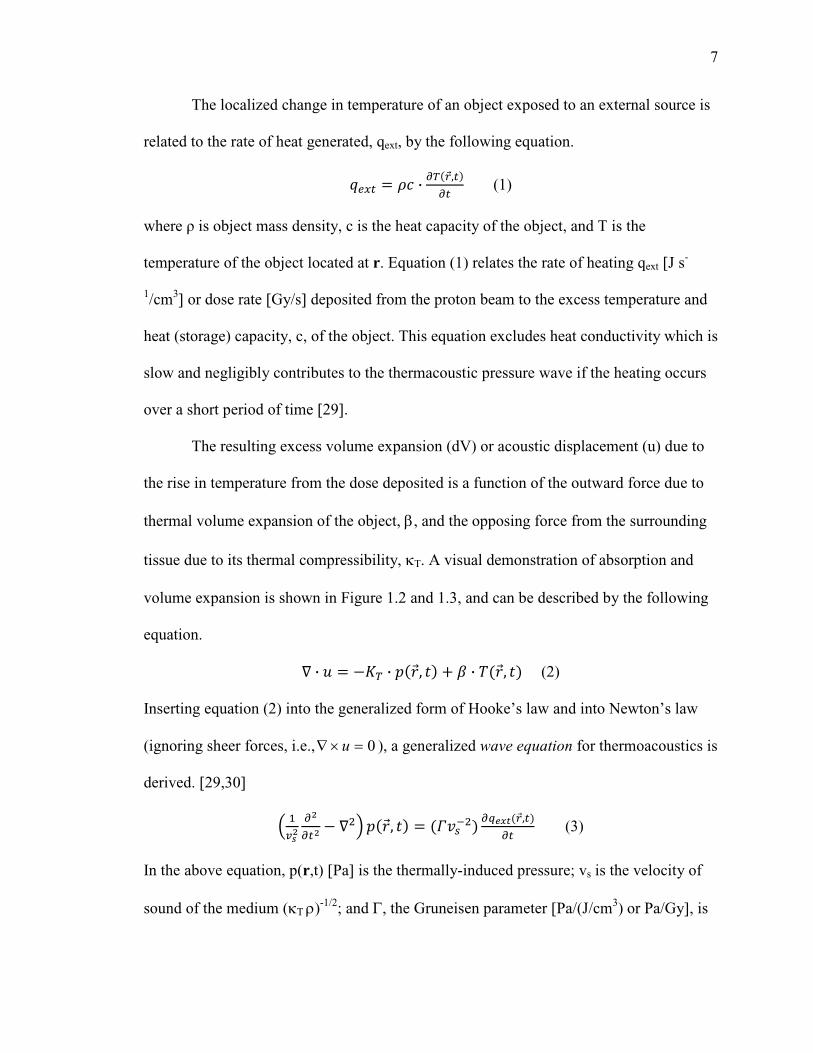
tissue due to its thermal compressibility, κT. A visual demonstration of absorption and

volume expansion is shown in Figure 1.2 and 1.3, and can be described by the following

equation.

· · , · , (2)

Inserting equation (2) into the generalized form of Hooke’s law and into Newton’s law

(ignoring sheer forces, i.e., 0=×∇ u ), a generalized wave equation for thermoacoustics is

derived. [29,30]

, !"#$ %&'( , (3)

In the above equation, p(r,t) [Pa] is the thermally-induced pressure; vs is the velocity of

sound of the medium (κT ρ)-1/2; and Γ, the Gruneisen parameter [Pa/(J/cm3) or Pa/Gy], is

8

equal to β c-1 (κTρ)-1. For tissue this parameter is about 1.3e5 Pa / (J/cm3) or 130 Pa/Gy,

and approximately 22 percent lower for water (107 Pa/Gy). The solution to equation (3)

is obtained using time-retarded Green’s function and its integration over all object space

d3r’.

, *·+

,- · . /0

1 $02222 1% ,

03$

1422 +402222 15

(4)

Figure 1.2 demonstrates the change in energy absorption.

9

Figure 1.3 Parameters in the Gruneiesen Coefficient

1.3 Imaging Techniques

The two imaging techniques were evaluated: the Computed tomography (CT) and

the Delay and Sum associated with a phased array. The emphasis is on the spherical

sampling space using the tomographic reconstruction. The investigation using the CT

imaging reconstruction is used in designing a Radiation Acoustics Computed

Tomography dosimeter/scanner (RACT). Once this dosimeter is constructed it can

provide in-vivo measurements of dose. Both of these imaging techniques can be used to

image 3D dosimetry.

10

1.3.1 Computed Tomography

From section 1.2, equation (3) can be recast into a form resembling a 3-

dimensional Radon transform,[29] where the projections as defined by the velocity

potential, φ(r,t), are related to the 2D surface integrals defined by the retarded time, |r-

r’|=vst. Given that p(t) = -ρ dφ/dt, we can write

6, 7 · 8 9:;

< (5)

Therefore, based on equations (4) and (5).

6, 7 · 8 9:9

< *+,-7 . /9

|$9| · , (6)

The rate at which the energy is absorbed, qext(r’,t), can be separated into a spatial and

temporal component Φ0D(r’)Τ(t’), where Φ0 is the proton particle flux, D(r’) is the

deposited dose, and Τ(t’) depicts the pulse shape of the proton beam. Assuming a

medium with a homogenous velocity of sound, the volume integral can be rewritten as a

surface integral over a spherical shell a distance r from the transducer.

If the proton beam is a rectangular pulse with a pulse width tPW, the above

equation resembles a 3-dimensional Radon transform. [29,31]

7 8 9>; ? *·+

,- · 6< · @A · "# B C9 |$9|3· · DE

(7)

In equation (7), the 1D projections, λn, for each transducer represents a 2D spherical

surface integral of the dose, D(r’).

λFG ,-7

*·+

HI·JK 8 9>; B C9 · >L

|$9|3· (8)

11

The reconstructed object is equivalent to the sum of overall projection angles and taking

the Laplacian,

M ,- · · 8 >ΩF ·

- λF N ,- 8 >ΩF ·

-OλP 1

|$9|3 (9)

The resulting 3D Radon transform can be written in the form of a filtered backprojection

algorithm where the projection data can be written as

λQ ? R · !$ · · STUVQW · XWY (10)

In the above equation, each projection depends on constants relating the thermoacoustic-

induced pressure to absorbed dose. g represents the total number of protons per pulse (Φ0

tPW) and a weighting factor wr’ for each projection, which depends on the geometry of the

scanner, i.e., uniformity of acquired projections. The parameter Γ is the factor

representing the effectiveness at which dose is converted to pressure based on the

physical properties of the object. The time t, is the propagation time of the pressure to

reach the transducer from within the object, providing an effective time-gain

compensation. P(w) is the measured pressure signal for a transducer. And, H(ω) is the

filter function,XW |W| · Z[\[ , where A(ω) is an apodizing function and I(ω) is the

impulse response of the transducer.

12

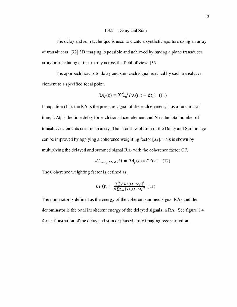
1.3.2 Delay and Sum

The delay and sum technique is used to create a synthetic aperture using an array

of transducers. [32] 3D imaging is possible and achieved by having a plane transducer

array or translating a linear array across the field of view. [33]

The approach here is to delay and sum each signal reached by each transducer

element to a specified focal point.

]^_ ∑ ]^a, ∆cd$c3< (11)

In equation (11), the RA is the pressure signal of the each element, i, as a function of

time, t. ∆ti is the time delay for each transducer element and N is the total number of

transducer elements used in an array. The lateral resolution of the Delay and Sum image

can be improved by applying a coherence weighting factor [32]. This is shown by

multiplying the delayed and summed signal RAf with the coherence factor CF.

]^ecfgD ]^_ h iT (12)

The Coherence weighting factor is defined as,

iT j∑ kZc,$∆lm+nloI j

d ∑ |kZc,$∆l|m+nloI

(13)

The numerator is defined as the energy of the coherent summed signal RAf, and the

denominator is the total incoherent energy of the delayed signals in RAf. See figure 1.4

for an illustration of the delay and sum or phased array imaging reconstruction.

13

Figure 1.4 Delay and Sum schematic

The delay and sum technique was tested using a point source, which was a nylon

monofilament with 1mm diameter inked with black marker. A linear array with 128

elements was used and a pulsed laser source. The reconstructed image shown in figure

1.5 had a Full Width Half Maximum (FWHM) of 1mm axially and 2 mm laterally.

Figure 1.5 The reconstruction of a point source located at 74 mm away from the transducer.

14

CHAPTER 2. METHODOLOGY

2.1 Simulations

The simulations of the acoustic pressure signal were written in IDL programming

language. A Monte Carlo (MC) dose distribution of a pulsed pencil proton beam was

used as an input to simulate on a voxel-by-voxel basis the thermoacoustic signal. The

geometry of the scanner is defined to find the time propagation to each transducer.

Different beam parameters – pulse width and rise time – were simulated to assess

sensitivity. Finally, an imaging reconstruction algorithm based on the three dimensional

(3D) filter back projection was developed and used to generate the images.

First, the simulation calculates the number of protons produced by setting the Pulse

Width (PW), Rise Time (RT), Beam Current [nano-Amperes], duty factor[%], and beam

width [FWHM]. The Monte Carlo simulated dose distribution data is then converted from

GeV/g to J/cm3 per proton. Total number of protons within a pulse is then calculated

using the PW, RT, beam current, and duty factor. The dose is calculated per voxel using

the MC data multiplied by the total number of protons.

15

2.2 Scanner Design

The geometry of the transducer array and a set of projections are displayed in

Figure 2.1. The transducer array consists of a 71 transducers along the surface of a

cylinder, with a length of 40cm and radius of 15cm. Each transducer is positioned along

the length of the cylinder (z-axis) and the end cap (x-axis), which is opposite to the

entrance of the proton beam, and its central axis intersecting the isocenter of the scanner

defined 20cm from the front surface along this central axis. The azimuthal sampling is set

to 2.5 degrees. To obtain a full set of projection angles, the scanner is rotated over 2π

every 10 degrees (total 36 angles).

Figure 2.1 The geometry of the transducer array used to simulate the excess pressure

created from the dose deposited from a proton beam.

16

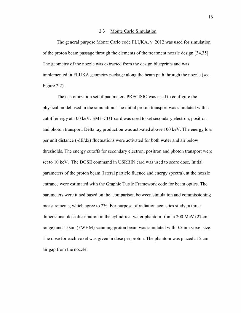
2.3 Monte Carlo Simulation

The general purpose Monte Carlo code FLUKA, v. 2012 was used for simulation

of the proton beam passage through the elements of the treatment nozzle design.[34,35]

The geometry of the nozzle was extracted from the design blueprints and was

implemented in FLUKA geometry package along the beam path through the nozzle (see

Figure 2.2).

The customization set of parameters PRECISIO was used to configure the

physical model used in the simulation. The initial proton transport was simulated with a

cutoff energy at 100 keV. EMF-CUT card was used to set secondary electron, positron

and photon transport. Delta ray production was activated above 100 keV. The energy loss

per unit distance (-dE/dx) fluctuations were activated for both water and air below

thresholds. The energy cutoffs for secondary electron, positron and photon transport were

set to 10 keV. The DOSE command in USRBIN card was used to score dose. Initial

parameters of the proton beam (lateral particle fluence and energy spectra), at the nozzle

entrance were estimated with the Graphic Turtle Framework code for beam optics. The

parameters were tuned based on the comparison between simulation and commissioning

measurements, which agree to 2%. For purpose of radiation acoustics study, a three

dimensional dose distribution in the cylindrical water phantom from a 200 MeV (27cm

range) and 1.0cm (FWHM) scanning proton beam was simulated with 0.5mm voxel size.

The dose for each voxel was given in dose per proton. The phantom was placed at 5 cm

air gap from the nozzle.

17

Figure 2.2 IU HPTC treatment nozzle model implemented on FLUKA CG geometry package.

2.4 Pressure Signal

To simulate the excess pressure, equation (4) from section 1.2 was integrated for

each transducer at each rotation angle, using a Γ of 1.0x105 [Pa/(J/cm3)], vs of 1.5mm/µs,

pulse width of 1µs, and 0.1µs risetime. The temporal properties of the pulsed proton

beam was modelled as a piece-wise linear function; therefore, the external source term

can represented by,

%&'(, pql,r,s·Ft

JKu∆∆ (14)

where kjiD ,,ˆ is the MC generated dose at each voxel in the water phantom, nP is the

number of protons within a pulse (1.8x107), tPW is the proton pulse width (at FWHM),

and ∆t the rise-time (in Figure 2.3 a 2µs tPW and 0.2µs ∆t is displayed). An acquisition

rate of 20MHz was used to digitally represent the pressure signal.

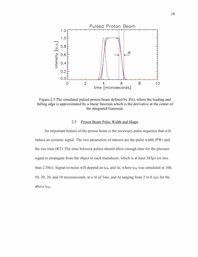
Figure 2.3 The simulated pulsed proton beam defined by falling edge is approximated by a linear function which is the derivative at the

2.5

An important feature of the proton beam is the necessary pulse sequence that will

induce an acoustic signal. The two parameters of interest are the pulse width (PW) and

the rise time (RT). The time between pulses should allow enough time for the pressure

signal to propagate from the object to each transducer, which is at least 385

than 2.5Hz). Signal-to-noise will depend on t

50, 30, 20, and 10 microseconds, at

above tPW.

The simulated pulsed proton beam defined by T(t), where the leading and falling edge is approximated by a linear function which is the derivative at the

the integrated Gaussian.

2.5 Proton Beam Pulse Width and Shape

An important feature of the proton beam is the necessary pulse sequence that will

induce an acoustic signal. The two parameters of interest are the pulse width (PW) and

(RT). The time between pulses should allow enough time for the pressure

signal to propagate from the object to each transducer, which is at least 385

noise will depend on tPW and ∆t, where tPW was simulated at 100,

and 10 microseconds, at a ∆t of 3ms, and ∆t ranging from 2 to 0.1

18

(t), where the leading and falling edge is approximated by a linear function which is the derivative at the center of

An important feature of the proton beam is the necessary pulse sequence that will

induce an acoustic signal. The two parameters of interest are the pulse width (PW) and

(RT). The time between pulses should allow enough time for the pressure

signal to propagate from the object to each transducer, which is at least 385µs (or less

was simulated at 100,

t ranging from 2 to 0.1µs for the

19

2.6 Ultrasound Transducers

To test the ultrasound transducers purchased from Olympus (immersion

transducers), a pulsed laser source is used. The Laser used is a Nd:YAG laser/OPO

(Quantel Brilliant, OPOTEK; 20ns pulses @20mJ) with beam width of 5mm. The

absorber point source was a black inked piece of tape. This will produce the impulse

response for the particular transducer as shown on Figure 2.4.

Figure 2.4 An impulse response (top) of 500kHz transducer with the frequency spectrum (bottom). The Gaussian fit of the spectrum (red dashed line) produced a center of 0.482

MHz and width of 0.226 MHz.

20

Then using a gamma variant function, other transducer center frequencies were

produced. For the scanner design, the impulse response of the transducers was simplified

using a flat frequency distribution with a wide bandwidth, which was realized using an

apodizing function (e.g., Butterworth filter) with a 1MHz cutoff frequency. To realize

this transducer response function, a combination of transducer elements can be

implemented, such as hydrophone in combination with a high frequency transducer or

multiple wide-band transducers.

Lastly, an experiment was conducted to acquire an energy calibration data for pulsed

laser beam source at five different energies. The readings were recording using a

spectrometer with units of mWatt. Then the ultrasound signal generated from each beam

is recorded using the 0.5MHz transducer with the black inked tape absorber. A set of data

demonstrating the signal to noise ratio SNR for this transducer using a pre-amplifier with

54 dB voltage gain and a bandwidth of 50 kHz to 5MHz was acquired. The five beam

energies were again used here.

21

CHAPTER 3. RESULTS

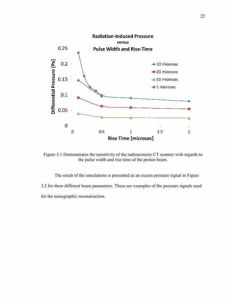
3.1 Pressure Signal

Based on equation (4) from section 1.2, the radiation-induce pressure signal, and

thus the sensitivity of radio-acoustic CT scanner, depends on both the pulse width (PW)

and rise time (∆t) of the proton beam. In Figure 3.1, the simulated pressure signal for

different PW and ∆t for the same number of protons (1.8x107) demonstrates that

compressing the protons in a shorter period of time (faster beam spill), can significantly

enhance the gain of the thermoacoustic signal and sensitivity to dose.

22

Figure 3.1 Demonstrates the sensitivity of the radioacoustic CT scanner with regards to the pulse width and rise time of the proton beam.

The result of the simulations is presented as an excess pressure signal in Figure

3.2 for three different beam parameters. These are examples of the pressure signals used

for the tomographic reconstruction.

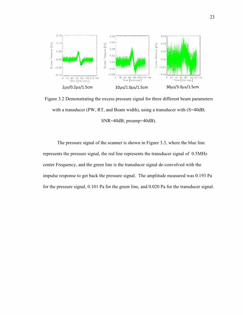
23

Figure 3.2 Demonstrating the excess pressure signal for three different beam parameters

with a transducer (PW, RT, and Beam width), using a transducer with (S=40dB;

SNR=40dB; preamp=40dB).

The pressure signal of the scanner is shown in Figure 3.3, where the blue line

represents the pressure signal, the red line represents the transducer signal of 0.5MHz

center Frequency, and the green line is the transducer signal de-convolved with the

impulse response to get back the pressure signal. The amplitude measured was 0.193 Pa

for the pressure signal, 0.101 Pa for the green line, and 0.020 Pa for the transducer signal.

24

Figure 3.3 Simulated Pressure signal for a Pulsed Proton beam with Pulse width of 1 micorsecond and Rise time of 0.1 microsecond.

3.2 RACT Signal Compared to Monte Carlo Dose

The 3D filtered backprojection algorithm was used to reconstruct the dosimetric

volume consisting of the Bragg peak, and compared to the MC results. A representative

slice along the x-z plane of the MC simulated proton beam and the reconstructed

radiation acoustic image is displayed in Fig.3.4 . A line plot along the central axis

demonstrates that the RA CT signal is within 2 percent of the MC generated dose within

the Bragg peak and distal edge, and linearity to dose (see Figure 3.5).

25

Figure 3.4 Displayed is the MC simulated dose (per proton) on a voxel-wise basis for a pencil proton beam with a range of 27cm in Water (left) and the reconstructed image from the radiation acoustic computed tomographic filtered backprojection algorithm (right), based on simulated thermoacoustic pressure signal.

26

Figure 3.5 Comparison of the MC dose to the RA CT signals along the central axis of the scanner.

The main issue seen in the line plot (Figure 3.5) is the decrease in signal at the

proximal end on the scanner. This is due to the non-uniform sampling of the scanner and

limited view projection angles. The range of the 90% dose is found to be 27.263 cm for

MC and 27.268 cm for the RACT signal. The peak range is 27.95 and 27.90 for MC and

RACT signal, respectively. A Gaussian fit of the Bragg peak expressed a width that is

0.3mm larger in the RACT signal compared to MC dose.

A density correction had to be applied to the reconstruction algorithm, where the

density is r/R. The term R is defined by the scanner diameter, which is 15.0cm. And r is

the calculated distance from each voxel to each transducer. This density factor corrects

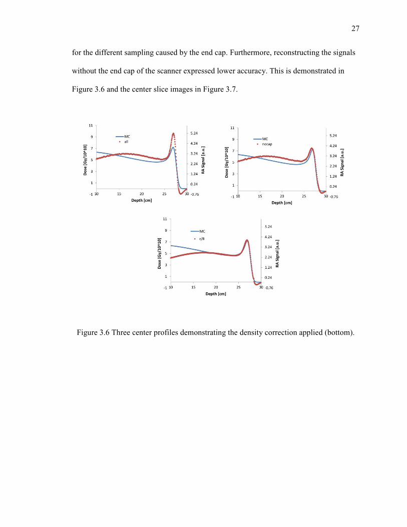
27

for the different sampling caused by the end cap. Furthermore, reconstructing the signals

without the end cap of the scanner expressed lower accuracy. This is demonstrated in

Figure 3.6 and the center slice images in Figure 3.7.

Figure 3.6 Three center profiles demonstrating the density correction applied (bottom).

28

Figure 3.7 RACT reconstructed images axially along the z-y plane. Left image was reconstructed without the endcap, center image was reconstructed without the density

correction, and finally the right image is reconstructed using a density correction.

Figure 3.8 Displays the RACT reconstructed images axially along the z-y plane and laterally along the x-y plane at the distal edge.

Lateral artefacts in the profile are found in figure 3.8 along z. Measurements of

the lateral dose as a function of range exhibits the lateral profile artifacts seen at the distal

edge (Figure 3.9).

29

Figure 3.9 Beam width as a function of range for Monte Carlo simulation and the RACT signals for Proton Beam with 27cm Range.

3.3 Transducer Results

The selection of the transducer type will depend on the properties of the beam and

the frequency components that will be measured. The low frequency components in a

pulsed proton source require lower center frequencies transducers. The frequency

components of Figure 3.3 are shown in Figure 3.6 in Decibel units. The bandwidth of a

500 KHz transducer was overlaid to demonstrate the acceptance of such transducer.

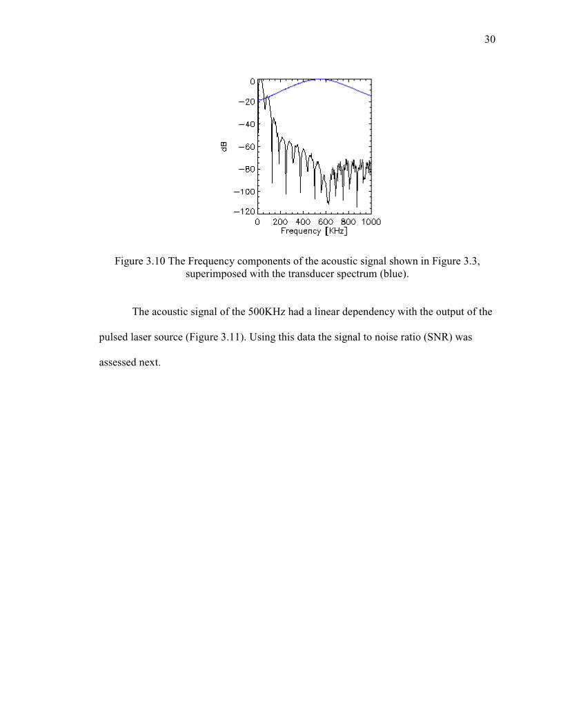
Figure 3.10 The Frequency components of the acoustic signal shown in Figure 3.3, superimposed with the transducer spectrum (blue).

The acoustic signal of the 500KHz

pulsed laser source (Figure 3.

assessed next.

The Frequency components of the acoustic signal shown in Figure 3.3, superimposed with the transducer spectrum (blue).

The acoustic signal of the 500KHz had a linear dependency with the output of the

pulsed laser source (Figure 3.11). Using this data the signal to noise ratio (SNR) was

30

The Frequency components of the acoustic signal shown in Figure 3.3,

had a linear dependency with the output of the

). Using this data the signal to noise ratio (SNR) was

31

Figure 3.11 Laser Calibration Data

The root mean square (RMS) was measured for each signal shown in Figure 3.12

to calculate the signal to noise ratio (SNR) and compared to the signal found recorded

using a pre-amplifier (see Figure 3.13). The results are shown in the tables below.

Table 3.1 The results of the signal recording using a 500kHz center frequency transducer.

RMS SNR=(rmsSignal/rmsNoise)

v1 0.00209 21.567

v2 0.00375 26.643

v3 0.00529 29.646

v4 0.00867 33.932

v5 0.01264 37.203

noise 1.74E-04

32

Table 3.2 The results of using a pre-amplifier with 54 dB gain.

Figure 3.12 Signals recorded using the pulsed laser source with increasing output.

RMS SNR=(rmsSignal/rmsNoise)

v1 0.6727 67.424

v2 1.1041 71.727

v3 1.2976 73.130

v4 1.5276 74.547

v5 1.7019 75.486

noise 2.86E-04

33

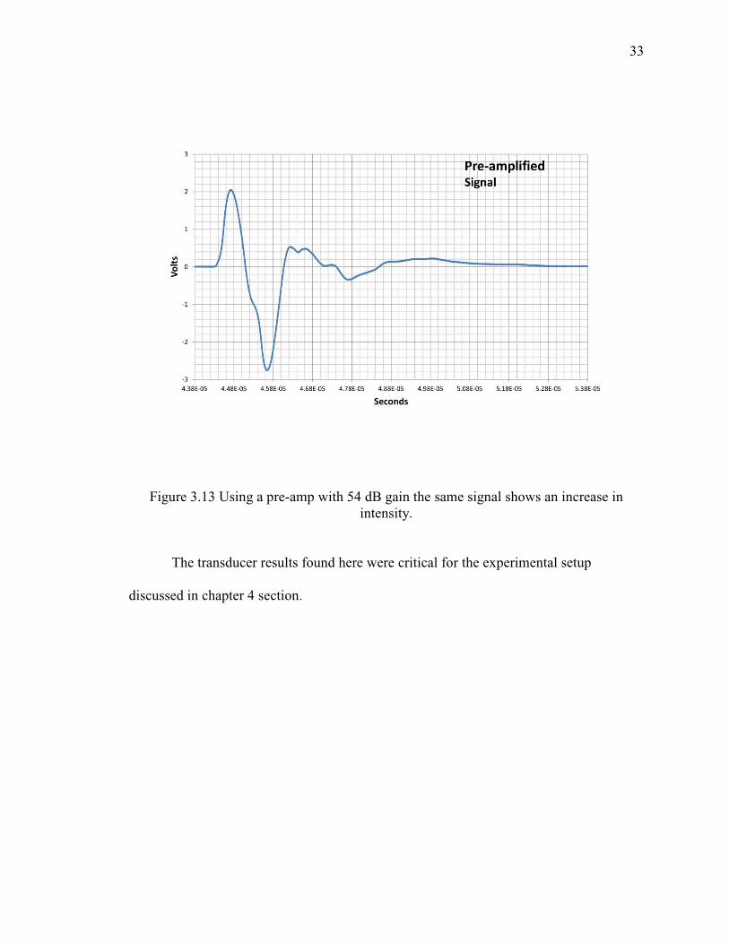
Figure 3.13 Using a pre-amp with 54 dB gain the same signal shows an increase in intensity.

The transducer results found here were critical for the experimental setup

discussed in chapter 4 section.

34

CHAPTER 4. CONCLUSION, DISCUSSIONS AND FUTURE AIMS

4.1 Feasibility

Current techniques, such as PET and PGs, have been shown to be able to locate

the distal edge of proton beams in phantoms with millimeter to a few millimeters

accuracy, respectively. However, due to the relatively high activation energy in the

formation of PET radioisotopes (11C, 14N, and 15O), the positron emitter signal does not

correspond well to the Bragg peak and location of the distal edge. Through the

implementation of analytical methods, such as Monte Carlo simulations or convolution of

treatment plan with filter functions, the distal fall-off and potentially the dose profile can

be obtained.[18] Even though 3-D images are readily obtained, the lack of sensitivity

requires in excess of 5Gy and the relatively long half-life of the radioisotopes makes

implementation very challenging.[18] Unlike PET, the PGs activation energy is

significantly lower and tracks the deposited dose more closely, to within 2-3mm of the

distal edge. However, PG activity when approaching the proton’s range decreases, as

does sensitivity and linearity. Extensive background from neutrons and stray gammas

limit the signal from higher energy PGs used to detect the edge. Recent simulated studies

in phantoms implementing camera designs, such as slit camera [37] and array-type

scintillator detectors,[10] have demonstrated the potential to determine the proton range

35

to within 1-2mm for doses ranging from 0.2-1Gy [10, 11, 37]. New detectors designs

using time-of-flight or Compton cameras are being investigated to suppress background

are being developed, and with the potential for 3-D image formation, may hold future

promise for PGs dosimetry and range verification.[18]

Many of the disadvantages associated with PET and PGs can be overcome with

radioacoustic imaging. Initial results based on RACT dosimetric scanner as presented in

2-D slice plane (Figure 3.4) demonstrates the 3-D imaging capabilities of a pulsed proton

beam within our scanner. Given that the radioacoustic signal is a direct measurement of

dose, a linear relationship between MC dose and RA CT intensities within the field of

view (FOV) of the scanner was observed (Figure 3.5), the location of the distal edge was

determined with sub-millimeter accuracy, and the dose within the Bragg peak was

determined to within 2 percent. The study done by Hayakawa T et al using a hydrophone

to measure the radioacoustic signal within a patient while undergoing proton beam

treatment measured a dose sensitivity of approximately 0.3cGy.[27] This suggests

radiation acoustic imaging can provide nearly two orders of magnitude better sensitivity

compared to current techniques, such as PGs. This would allow for pulse-wise

measurements of the proton beam range and dose during therapy.

Unlike PET or PGs, the proton beam profile and delivery are important factors

when considering radioacoustic sensitivity, as demonstrated in Figure 3.1. These factors

include the temporal properties of the pulsed proton beam, as well as the scanner

geometry. From equations (4) and (11) in chapter 1, section 2, the radiation-induced

pressure, and thus RACT intensity, is the integral of the pressure signals from the dose

deposited that is weighted by the inverse of proton beam pulse width (tPW), rise-time (∆t),

36

and propagation distance. Therefore, when comparing radioacoustic sensitivities, the dose

per pulse will need to be normalized relative to tPW and ∆t for a given scanner geometry.

For example, the study by Hayakawa T et al used a 50nsec pulse width, which would

significantly increase radioacoustic pressure (based on Figure 3.1). An advantage of the

RACT dosimetric scanner design is that it acquires thousands of projection angles, thus

enhancing the signal-to-noise and providing comparable or better sensitivities over a

wide range of proton beam pulses.

The future aims once the RACT scanner is fabricated is to achieve the verification

of the position of distal edge within 2mm, have a spatial resolution of less than 2mm, and

less than 5% dose variation between measurements and actual dose. Before translating

the scanner to a clinical setting, the effects of the heterogeneous acoustic properties of

tissue and limited angular coverage consistent with a patient will be measured.

Corrections to the reconstruction algorithm for acoustic tissue properties, including

speed-of-sound, attenuation, and impedance, using tissue phantom will be tested in the

proton beam. Simulations based on geometric limitation observed in the clinic will be

performed. Combined, RACT designs that can be translated to the clinical will be will be

investigated. Initially, RACT scanner can be used as a treatment verification tool.

4.2 IU Blomington Proton Facility Experiment

The primary objective of this experiment is to observe an acoustic signal generated

by a pulsed proton beam. A transducer is translated on a linear stage to obtain data

representing a linear transducer array. Image reconstruction of the linear array data is

then conducted. However, modifications were made during the experiment because of the

37

expected low current, and pulse width and rise time properties of the proton beam. This

section will present the experimental set up for any proton facility in the future. It also

emphasizes the importance of simulating results prior to performing an experiment for

different proton facilities depending on their proton accelerator capabilities.

4.2.1 Methods

The initial setup used a water tank phantom with a linear translation system (LTS)

mounted on the top of the tank. It is positioned so that the center of the tank lines up with

the center range of motion of the LTS. The LTS had a range of 100mm. The transducer is

attached to the LTS and constructed to point downward in the tank at a distance of 45

mm away from the axis of the beam as shown in figure 4.1. This is done to be in the far

field for the transducers used (center frequencies of 0.5MHz, 1MHz, and 2.25MHz).

Alignment set up provided by the proton facility was used to have the center of the

Bragg-peak at the center of the water tank.

The near field and divergence angle calculation used were, N p_,w , where N is

the near field distance, D is the diameter, f is the operating frequency, and c is the speed

of sound in water (1500 m/s), and x yza|. wp_ , angle of

divergence (far field). [37]

38

List of transducers used in the experimetn with near field and divergence angles

calculations:

1) Transducer f=2.25 MHz D=10mm

N = 37.5mm and θ = 4.665o

2) Transducer f=1.00 MHz D=13mm

N = 28.17mm and θ = 8.092o

3) Transducer f=0.50 MHz D=19mm

N = 30.08mm and θ = 11.106o

Figure 4.1 Water Tank Phantom to position and translate the ultrasound transducer.

39

The instrumentations used were:

o Piezoelectric transducers.

Linear array transducer with 128 elements at 0.3mm pitch from acuson

model L538.

Three transducers with 0.5, 1.0, and 2.25 MHz center frequencies

unfocused made by Olympus Corporation. Part IDs (U8423005,

U8423053, U8423038)

o Linear stepper motor with high resolution steps (LTS) [Newmark systems inc.

model eTrack] .

o Pre-Amplifier Model 5662 Olympus, with 34 dB and 54 dB voltage gain and a

bandwidth of 50 kHz to 5MHz.

o Water tank.

o Thermostat.

o Proton detector triggers.

o Oscilloscope with LAN connection to a computer.

o Lead shielding to protect equipment in the room.

o Pulsed Laser source for initial checks.

The experiment followed a procedural guide book and as mentioned above

modified in expectations to low signals. The modification consisted of using a 4mm lead

40

sheet in the direction of the proton beam, with the ultrasound transducer positioned at

4cm away from the lead sheet. The lead sheet was positioned at 26 cm away from the

edge of the water tank. This is demonstrated in Figure 4.2.

Figure 4.2 The experiment modification using a lead sheet.

First Step: System Set up and checks

The instrumentation is set up in the proton room provided and checked using a

pulsed laser source to observe a signal before the start of the experiment. A thermostat is

used to measure the temperature of the water. This reading should remain constant during

data acquisition, as changes in the temperature from the proton beam are anticipated to be

small. The LTS function was tested with the software provided. The oscilloscope

connection with LAN network was tested to obtain an IP address. Then using NI MAX

software a connection is established with the IP address. Data acquisition was saved on

the operating computer using “get function” from Tektronix OpenChoice Software. The

settings can be sent to the oscilloscope using “set function”. See figure 4.3. The

41

transducers are checked with the pulsed laser source and an absorbing material in the

water to check the ultrasound signal as shown in figure 4.4. An alternative method for

data acquisition is using the IP address in a web browser.

Figure 4.3 Tektronix OpenChoice Desktop Software is used to send settings and acquire data.

Figure 4.4 An ultrasound signal recorded using the oscilloscope and triggered using the laser. Approximate position of the transducer was 15 mm.

Second Step: Alignment setup and signal check from proton beam.

42

Alignment of the water tank with beam axis to the center and at a distance of

45mm away from transducer was setup with assistance of beam lasers. The Bragg peak is

centered with the 0.5MHz transducer. The oscilloscope is connected to the trigger that

would define when the beam is on. This is used to calculate the distance of the proton

beam to the transducer which should be 45 mm. The oscilloscope is set to take 128

averages and record it using the “get function”. Then, the transducer is moved away from

the beam toward the end of the distal edge and data is recorded. From these two points

we can confirm that we are seeing a signal and can measure the distance to the transducer.

Third Step: Translation experiment.

Once we have determined that a signal is observable, the transducers mounted on the

LTS will translate along the beam to record the shape of the proton beam; Bragg peak

and distal edge. The Proton beam peak is aligned at the center of the tank. The LTS

system will be positioned at 20 mm away from the peak. The beam is turned on and the

LTS system will move in steps of 5mm to record the shape of the beam toward the peak

and record a total of 10 steps (Length of 40mm). Each step is recorded and saved on the

computer in a step and shoot fashion. This will lead to a recording of a linear array.

However, this step was not conducted because of the experiment modification.

4.2.2 Results and Conclusion

The temperature reading of the water tank was initially at 27.0 Co and dropped to

24.8 Co. The last temperature reading did not vary throughout the experiment. The proton

beam energy was 204.9 MeV and the beam current was 70 nAmp. The proton beam

43

structure is shown in Figure 4.5 As anticipated the modifications on this experiment had

to be done to see a signal. The 4 mm lead sheet used showed a very small signal (<0.5

mVolts) Figure 4.6.

Figure 4.5 Proton beam structure from Indiana Proton Therapy Center

Figure 4.6 Signal response of 0.5 MHz Transducer positioned 4 cm away from the lead sheet.

The beam parameters and shape of this experiment are used to simulate what the

pressure signal would be in water. The transducer is placed at 3cm away from the Bragg

Peak centered axially along the beam. The simulated transducer signal was 0.00005 Pa

(Red line, Figure 4.7), and the pressure signal was 0.0005 Pa (Blue line, Figure 4.7). This

is deemed unmeasurable and insignificant compared to the background noise.

Figure 4.7 Simulation of Bloomington Experiment using the Water Phantom. The Blue line is the simulated pressure signal and the red line is the transducer signal (500kHz, 50%

These results emphasize

sequence and shape as discussed in the simulations (section 2.1) above. This expe

will be used as a first step

other proton beam facilities

acquisition system coupled with automatic software that translates and records signals

automatically. Once a set of linear array data are recorded the Delay and Sum can be

implemented during the ex

done after the experiment completion.

(Red line, Figure 4.7), and the pressure signal was 0.0005 Pa (Blue line, Figure 4.7). This

is deemed unmeasurable and insignificant compared to the background noise.

Simulation of Bloomington Experiment using the Water Phantom. The Blue line is the simulated pressure signal and the red line is the transducer signal (500kHz, 50%

Bandwidth).

These results emphasize the importance on sensitivity with the proton pulse

sequence and shape as discussed in the simulations (section 2.1) above. This expe

first step to validate simulation code and as a baseline when comparing

other proton beam facilities. Data acquisition can be improved by using a standalone data

acquisition system coupled with automatic software that translates and records signals

automatically. Once a set of linear array data are recorded the Delay and Sum can be

implemented during the experiment for a quick image display. Further analysis should be

done after the experiment completion.

44

(Red line, Figure 4.7), and the pressure signal was 0.0005 Pa (Blue line, Figure 4.7). This

is deemed unmeasurable and insignificant compared to the background noise.

Simulation of Bloomington Experiment using the Water Phantom. The Blue line is the simulated pressure signal and the red line is the transducer signal (500kHz, 50%

mportance on sensitivity with the proton pulse

sequence and shape as discussed in the simulations (section 2.1) above. This experiment

to validate simulation code and as a baseline when comparing

ata acquisition can be improved by using a standalone data

acquisition system coupled with automatic software that translates and records signals

automatically. Once a set of linear array data are recorded the Delay and Sum can be

periment for a quick image display. Further analysis should be

45

4.3 Proton Facilities

The importance of a pulse sequence will affect the type of accelerators and their

capabilities to induce an acoustic signal. The most promising choice for a new accelerator

system is a superconducting synchrocyclotron (SCSC). [38, 39] The superconducting

synchrotron has many attractive features, including low cost and ease of operation

(allowing for full automation) which, along with the use of superconducting magnet

gantries and permanent magnet beam transport lines will make possible to reduce the

capital cost of proton systems to be competitive with that of advanced x-ray systems and

ensure that SCSC will play a significant role in the transition to a next generation of

proton therapy equipment. Its beam structure of one to several microsecond pulses at a

rate of up to 1000 pulses per second is well suited for 3D dose imaging applications

utilizing radiation acoustics. In addition, there are long term efforts on developing other

advanced acceleration technology [39, 40] based on either a high gradient dielectric wall

accelerator [41] or a laser driven medical accelerator [42-44]. These systems all would

have a pulsed beam with very short pulses and high fluences ideal for radiation-induced

acoustic imaging.

4.4 Conclusion

This feasibility study demonstrates that RACT can be used to monitor the dose

distribution and proton range in proton therapy. The ability to non-invasively image the

dose distribution in a patient, the accuracy and precision of the treatment plan can be

determined, and potentially modified or adapted over the time of the therapy. Design and

construction of a phantom to obtain measured data, and comparison to simulated data is a

work in progress.

LIST OF REFERENCES

46

LIST OF REFERENCES

1. Kataria T, Rawat S, Sinha SN, et al. Dose reduction to normal tissues as compared to the gross tumor by using intensity modulated radiotherapy in thoracic malignancies. Radiation Oncology. 2006;1:31.

2. Miralbell R, Lomax A, Cella L, et al. Potential reduction of the incidence of radiation-induced second cancers by using proton beams in the treatment of pediatric tumors. Int. J. Radiat. Oncol. Biol. Phys. 2002;54:824–829.

3. Merchant TE, Hua C-H, Shukla H, et al. Proton versus photon radiotherapy for common pediatric brain tumors: comparison of models of dose characteristics and their relationship to cognitive function. Pediatr Blood Cancer. 2008;51:110–117.

4. Paganetti H, van Luijk P. Biological Considerations When Comparing Proton Therapy With Photon Therapy. Seminars in Radiation Oncology. 2013;23:77–87.

5. Simone CB 2nd, Kramer K, O’Meara WP, et al. Predicted rates of secondary malignancies from proton versus photon radiation therapy for stage I seminoma. Int. J. Radiat. Oncol. Biol. Phys. 2012;82:242–249.

6. Foote RL, Stafford SL, Petersen IA, et al. The clinical case for proton beam therapy. Radiat Oncol. 2012;7:174Schneider U, Sumila M, Robotka J. Site-specific dose-response relationships for cancer induction from the combined Japanese A-bomb and Hodgkin cohorts for doses relevant to radiotherapy. Theor Biol Med Model. 2011;8:27.

7. Paganetti H, Athar BS, Moteabbed M, et al. Assessment of radiation-induced second cancer risks in proton therapy and IMRT for organs inside the primary radiation field. Phys Med Biol. 2012;57:6047–6061.

8. Vynckier S, Derreumaux S, Richard F, et al. Is it possible to verify directly a proton-treatment plan using positron emission tomography? Radiother Oncol. 1993;26:275–7.

9. Min CH, Lee HR, Kim CH, et al. Development of array-type prompt gamma measurement system for in vivo range verification in proton therapy. Medical Physics. 2012;39:2100–2107.Min C-H, Kim CH, Youn M-Y, et al. Prompt gamma measurements for locating the dose falloff region in the proton therapy. Applied Physics Letters. 2006;89:183517.

10. Zhu X, Fakhri, GE. Proton Therapy Verification with PET Imaging. Theranostics. 2013;3:731–740.

47

11. Parodi K, Bortfeld T. A filtering approach based on Gaussian-powerlaw convolutions for local PET verification of proton radiotherapy. Phys Med Biol. 2006;51:1991–2009.

12. Attanasi F, Knopf A, Parodi K, et al. Extension and validation of an analytical model for in vivo PET verification of proton therapy--a phantom and clinical study. Phys Med Biol. 2011;56:5079–5098.

13. Oelfke U, Lam GK, Atkins MS. Proton dose monitoring with PET: quantitative studies in Lucite. Phys Med Biol. 1996;41:177–196.

14. Knopf A-C, Parodi K, Paganetti H, et al. Accuracy of proton beam range verification using post-treatment positron emission tomography/computed tomography as function of treatment site. Int. J. Radiat. Oncol. Biol. Phys. 2011;79:297–304.

15. Parodi K, Paganetti H, Shih HA, et al. Patient study of in vivo verification of beam delivery and range, using positron emission tomography and computed tomography imaging after proton therapy. Int. J. Radiat. Oncol. Biol. Phys. 2007;68:920–934.

16. Knopf A-C, Lomax A. In vivo proton range verification: a review. Phys Med Biol. 2013;58:R131–160.

17. Moteabbed M, España S, Paganetti H. Monte Carlo patient study on the comparison of prompt gamma and PET imaging for range verification in proton therapy. Physics in Medicine and Biology. 2011;56:1063–1082.

18. Chu WT, Ludewigt BA, Renner TR. Instrumentation for treatment of cancer using proton and light‐ion beams. Review of Scientific Instruments. 1993;64:2055–2122.

19. Robertson D, Hui C, Archambault L, et al. Optical artefact characterization and correction in volumetric scintillation dosimetry. Phys Med Biol. 2014;59:23–42.

20. Albul VI, Bychkov VB, Vasil’ev SS, et al. Acoustic field generated by a beam of protons stopping in a water medium. Acoust. Phys. 2005;51:33–37.

21. Xiang L, Han B, Carpenter C, et al. X-ray acoustic computed tomography with pulsed x-ray beam from a medical linear accelerator. Med Phys. 2013;40:010701.

22. Sulak L, Armstrong T, Baranger H, et al. Experimental studies of the acoustic signature of proton beams traversing fluid media. 1979;161:203–217.

23. De Bonis G. Acoustic signals from proton beam interaction in water—Comparing experimental data and Monte Carlo simulation. Nuclear Instruments and Methods in Physics Research Section A: Accelerators, Spectrometers, Detectors and Associated Equipment. 2009;604:S199–S202.

24. Tada J, Hayakawa Y, Hosono K, et al. Time resolved properties of acoustic pulses generated in water and in soft tissue by pulsed proton beam irradiation—A possibility of doses distribution monitoring in proton radiation therapy. Medical Physics. 1991;18:1100–1104

48

25. Hayakawa Y, Tada J, Arai N, et al. Acoustic pulse generated in a patient during treatment by pulsed proton radiation beam. Radiation Oncology Investigations. 1995;3:42–45.

26. Lyamshev LM. Radiation acoustics. Boca Raton, Fla.: CRC Press; 2004.

27. Kruger RA, Liu P, Fang YR, et al. Photoacoustic ultrasound (PAUS)--reconstruction tomography. Med Phys. 1995;22:1605–1609.

28. Kruger RA, Liu P. Photoacoustic ultrasound: pulse production and detection of 0.5% Liposyn. Med Phys. 1994;21:1179–1184.

29. Yuan Y, Xing D, Xiang L. High-contrast photoacoustic imaging based on filtered back-projection algorithm with velocity potential integration. In: Vol 7519.; 2009:75190L–75190L–8.

30. Liao C-K, Li M-L, Li P-C. Optoacoustic imaging with synthetic aperture focusing and coherenceweighting. Opt. Lett. 2004;29:2506–2508.

31. Zhou Q, Ji X, Xing D. Full-field 3D photoacoustic imaging based on plane transducer array and spatial phase-controlled algorithm. Medical Physics. 2011;38:1561–1566.

32. Battistoni G, Cerutti F, Fassò A, et al. The FLUKA code: description and benchmarking. AIP Conference Proceedings. 2007;896:31–49.

33. Ferrari A, Ranft J, Sala PR, et al. FLUKA.; 2005.

34. Smeets J, Roellinghoff F, Prieels D, et al. Prompt gamma imaging with a slit camera for real-time range control in proton therapy. Phys Med Biol. 2012;57:3371–3405.

35. Bushberg JT. The essential physics of medical imaging. Philadelphia: Wolters Kluwer Health/Lippincott Williams & Wilkins; 2012.

36. Matthews JN. Accelerators shrink to meet growing demand for proton therapy. Physics Today. 2009;62:22.

37. Peggs S, Satogata T, Flanz J. A survey of hadron therapy accelerator technologies. In: Particle Accelerator Conference, 2007. PAC. IEEE.; :115–119.

38. Flanz J, Smith A. Technology for proton therapy. Cancer J. 2009;15:292–7.

39. Caporaso GJ, Mackie TR, Sampayan S, et al. A compact linac for intensity modulated proton therapy based on a dielectric wall accelerator. Phys Med. 2008;24:98–101.

40. Linz U, Alonso J. What will it take for laser driven proton accelerators to be applied to tumor therapy? Physical Review Special Topics - Accelerators and Beams. 2007;10:094801.

49

41. Murakami M, Demizu Y, Niwa Y, et al. Current Status of the HIBMC, Providing Particle Beam Radiation Therapy for More Than 2,600 Patients, and the Prospects of Laser-Driven Proton Radiotherapy. In: Dössel O, Schlegel WC, eds. World Congress on Medical Physics and Biomedical Engineering, September 7 - 12, 2009, Munich, Germany. IFMBE Proceedings. Springer Berlin Heidelberg; 2009:878–882.

42. Schwoerer H, Pfotenhauer S, Jackel O, et al. Laser-plasma acceleration of quasi-monoenergetic protons from microstructured targets. 2006;439:445–44