fear and economic behavior
TRANSCRIPT

Fear and Economic Behavior
Lina Andersson∗
October 22, 2021
Abstract: Fear is an important factor in decision making under risk anduncertainty. Psychology research suggests that fear influences one’s risk attitudeand fear may have important consequences for decisions concerning for exampleinvestments, crime, conflicts, and politics. I model strategic interactions betweenplayers who can be either in a neutral or a fearful state of mind. A player’sstate of mind determines his or her utility function. The two main assumptionsare that (i) fear is triggered by an increase in the probability or cost of negativeoutcomes and (ii) a player in the fearful state is more risk averse. A player’s be-liefs over the probability and cost of negative outcomes determine how the playertransitions between the states of mind, and I use psychological game theory toanalyse three applications. The applications illustrate how fear of a bank runcan spread among bank clients and cause a bank panic, how a player can useknowledge of others’ fear sensitivity to own advantage, and how fear can causean apparent overreaction to bad news.
Keywords: emotions; fear; risk aversion; psychological game theory
JEL Classification: C72; D01; D91
∗Department of Economics, University of Gothenburg; e-mail: [email protected]. I am grateful for advice from Li Chen, Martin Dufwenberg, Claes Ek, RachelMannahan, Katarina Nordblom, Ernesto Rivera Mora and Jörgen Weibull. I also thank theparticipants of the Behavioral Economics seminar in Gothenburg, 2020, and the participantsof the Queen Mary University of London Economics and Finance Workshop for their helpfulcomments and feedback.
1

1 Introduction
Fear influences one’s judgement, behavior, and decision making. A fearful personshows an increased concern with risk and tends to be less willing to participatein risky lotteries. For instance, a person who becomes fearful after an extremestock market fall may overreact and sell more than he or she otherwise wouldhave. Although fear is an important factor in decision making under risk anduncertainty, few economists have studied the topic and a formal analysis of thebehavioral consequences of fear remains absent.1
This paper proposes a game theoretic model of players who can transition froma neutral to a fearful state of mind. A player’s state of mind determines his or herutility function. While fear can manifest itself in many ways, in this paper fearis defined as an emotion with a specific trigger and which causes an increasedconcern with risk.2 More specifically, the assumption is that a player is morerisk averse in the fearful than in the neutral state of mind. By focusing on thebehavioral consequences of fear as mediated through an increased risk aversion,I abstract from the negative utility from the experience of fear. I assume that aplayer transitions to the fearful state of mind after an increase in the probabilityor cost of negative outcomes. A negative outcome is an outcome bad enough topotentially instill fear when anticipated.
The players hold initial beliefs over the expected cost of negative outcomeswhen the game begins. A player transitions to the fearful state of mind afteran increase in the expected cost of negative outcomes. Since the players’ beliefsdirectly affect their utility functions, the game is a psychological game (Battigalli& Dufwenberg, 2009; Battigalli et al., 2019).3 Consider for example a person whotakes a walk in the park late at night. A negative outcome in this interaction
1The interest for fear and decision making has grown among empirical and experimentaleconomists during the decade since the financial crisis (see e.g. Callen et al., 2014; Campos-Vazquez & Cuilty, 2014; Cohn et al., 2015; Dijk, 2017; Guerrero et al., 2012; Guiso et al.,2018; Kuhnen & Knutson, 2011; Malmendier & Nagel, 2011; Nguyen & Noussair, 2014; Wang& Young, 2020). The relationship between fear and risk attitudes is not found in all papers(see e.g. Alempaki et al., 2019; Gärtner et al., 2017).
2Psychology literature emphasize that once an individual becomes fearful, his or her concernwith risk increases Holtgrave & Weber (see e.g. 1993); Lerner & Keltner (see e.g. 2000, 2001);Lerner et al. (see e.g. 2003); Loewenstein et al. (see e.g. 2001); Smith & Ellsworth (see e.g.1985); Smith & Lazarus (see e.g. 1991).
3For a general discussion of psychological game theory and its usefulness in modeling emo-tions and other belief-dependent motivations, see e.g. Battigalli & Dufwenberg (2020).
2

is to be robbed of all of one’s money and one may become fearful if a strangerapproaches.
The role of fear is illustrated in three applications. The first application isa sequential game between a robber and a victim. This game illustrates how aplayer may use his or her knowledge of another player’s fear sensitivity to bringabout a desired outcome when the players’ incentives are misaligned. The secondis a simplified version of Diamond & Dybvig’s (1983) seminal bank run game withthe addition of an exogenous risk that a player ‘needs money tomorrow’ and isforced to withdraw. This game illustrates how fear can affect the outcome alsowhen players’ incentives are aligned, and how fear of a bank run can spread ina population and cause a bank run. The third application illustrates how fearmay affect a player’s willingness to take a vaccine when a public health authorityinforms him or her about a disease. This application highlights the tendency offear to strengthen a player’s response to information that increases the probabilityor cost of negative outcomes.
The observation that fear can be of importance in strategic interactions hasbeen made before. Shelling (1980) discusses the strategic consequences of fear ina situation similar to the robbery game studied in this paper. Shelling considersa homeowner who investigates a noise at night with a gun in his hand, just to finda burglar, also armed with a gun. The situation has two equilibria. In one, noone shoots and the burglar leaves quietly. In the other, the homeowner and theburglar shoot each other. While neither of them prefers the shooting equilibria,Shelling notes that they may shoot not by calculation, but by nervousness. Thissituation can be formalized using the model proposed in this paper. If either thehomeowner or the burglar were to become fearful, then shooting becomes theunique equilibrium.
Psychological game theory has been used to model other emotions, for exam-ple guilt and anger (Battigalli & Dufwenberg, 2007; Battigalli et al., 2019). Intu-itively, anger is the emotion most closely related to fear. Battigalli et al. (2019)model players with a belief-dependent utility function that assigns a weight bothto own and others’ material payoff. In the absence of frustration, the weight onothers’ material payoff is zero. However, as a player’s expected material payoffdecreases, his or her frustration increases. As frustration increases, the player’snegative concern for others’ payoffs increases. Similar to the players studied in
3

this paper, the players in (Battigalli et al., 2019) form initial beliefs over howthe interaction will play out, and a disadvantageous change alters their utilityfunction. However, Battigalli et al. study players who become frustrated iftheir expected material payoff decreases, whereas this paper studies players whotransition to a fearful state of mind if their expected cost of negative outcomesincreases. Moreover, while the triggers of frustration and fear are similar, frus-tration causes a player to have a negative concern for others’ payoffs whereas fearcauses an increased concerned with risk.
Caplin & Leahy (2001) propose a model of anticipatory emotions. They studya two-period model of lotteries with a mapping from physical lotteries to mentalstates. The decision maker’s first-period utility may for example decrease in thevariance of the second-period realizations of the lottery. Such a decision maker issaid to experience anxiety prior to the resolution of the lottery and is less likelyto take part in lotteries with high variance. By contrast, the focus of this paperis on the increased concern with risk in the fearful state of mind.
Another closely related paper is Kőszegi & Rabin (2007). Kőszegi & Rabinbuild on Kahneman & Tversky’s (1979) work on prospect theory. They model adecision maker who evaluates an outcome relative to a reference point formed bythe decision makers recent beliefs. The decision maker’s utility is a combinationof a reference-independent “consumption utility” and a “gain loss” utility thatdepends on the difference between the consumption utility and the referencepoint.
The decison maker’s reference point determines how much risk he or she iswilling to take on. The reference point can be either deterministic or stochastic.A decision maker who expects risk views a lottery as less aversive than a decisionmaker who does not expect risk to start with. Moreover, the decision maker issophisticated in the sense that he or she correctly predicts the environment andown behavior in the environment.
Similarly, in this paper a player’s transition to the fearful state of mind de-pends on the player’s initial beliefs over how the interaction will play out. Theplayers are also sophisticated in the sense that they can correctly predict ownand others’ state transitions and the behavioral consequences. However, whileKőszegi & Rabin’s decision maker has a reference-dependent utility function, theplayers in my model have belief-dependent transition probabilities between their
4
states of mind. Further, Kőszegi & Rabin’s decision maker is concerned withexpected consumption utility and any deviations therefrom, whereas the playersin this paper are concerned with the expected cost of negative outcomes.
Dillenberger & Rozen (2015) also study decision makers whose risk attitudemay change during the decision making process. They model a decision makerwho makes repeated decisions over lotteries. The decision maker becomes morerisk averse after a disappointing realization than after an elating. Realizationsare classified as disappointing or elating using a threshold rule. By contrast, thispaper studies players who may transition to a fearful state of mind when theexpected cost of negative outcomes increases.
This paper proceeds as follows. Section 2 presents the model and preliminariesof psychological game theory. Sections 3, 4, and 5 apply the model to threeinteractions, a robbery game, a bank run game, and a public health intervention.Section 6 discusses the model and concludes.
2 The Model
2.1 Preliminaries
Game form The focus of this paper is on a class of finite multi-stage gameforms with observed actions and perfect recall.4 Let I = {1, ..., n} denote thefinite set of personal players. The game form may contain chance moves ormoves by “nature” denoted by player 0. Let I0 = I ∪ {0}.
The multi-stage game consists of L + 1 stages indexed by l ∈ {0, ..., L}. Atthe end of each stage, all players observe the stage’s action profile. Let a0 ≡(a0
0, a01, ..., a
0n) be the stage-0 action profile. At the beginning of stage 1, players
know history h1, which can be identified with a0. Similarly, define hl+1, thehistory at the end of stage l, to be the sequence of actions in the previous periods,hl+1 = (a0, a1, ..., al). Let the initial, or empty, history be denoted by h0, the setof non-terminal histories denoted by H, and let the set of terminal histories, orplays, hL+1, be denoted by Z.
Let Ai(hl) denote the feasible actions of player i ∈ I in stage l when thehistory is hl, and let A(hl) = ×i∈IAi(hl). In each stage the players, including
4A game form (or a game protocol) specifies the structure of a strategic situation: theplayers, how they can choose, and the material consequences of their actions.
5

chance, simultaneously choose actions from a finite subset of (potentially) history-dependent feasible actions Ai(hl). This can be done without loss of generalitysince an inactive player can be represented as a player whose feasible action Ai(hl)is a singleton with “do nothing” as the only action.
If chance is active at hl, its move is specified by the probability mass functionp0(·|h) ∈ ∆(A0(hl)). Chance selects a feasible action at random, and the actionis revealed to the players after the stage. The players have identical priors on theprobability of chance’s actions.
The material payoffs of the players’ actions are determined by an outcomefunction π : Z → Rn that associates each play z with a profile of material payoffs.
Beliefs Players form beliefs over own and others’ behavior, and over others’beliefs about behavior. A player’s beliefs are modeled as a hierarchical conditionalprobability system (Battigalli et al., 2019). A player’s beliefs over own and other’sbehavior – the plays z ∈ Z – are called first-order beliefs. They are definedfor each history h ∈ H. The first-order beliefs are denoted by αi(·|Z(h)) ∈∆(Z(h)), where ∆(Z(h)) is the set of probability measures on Z(h). The systemof beliefs αi = (αi(·|Z(h)))h∈H must satisfy two properties. First, Bayes’ rulefor conditional probabilities must hold whenever defined. Second, if in stage lplayer i moves simultaneously with other players, then i must believe that thesimultaneous actions of the co-players are statistically independent of i’s action.5
The first-order beliefs αi, are composed of two parts: player i’s beliefs over ownand over other’s behavior. The beliefs over own behavior, αi,i ∈ ×h∈H∆(Ai(h)),take the form a behavior strategy. They can be interpreted as the player’s plansince they are the result of the player’s contingent planning of which action totake at each history.6
A player’s beliefs over other players’ first-order beliefs constitute his or hersecond-order beliefs. Let ∆i,1 denote player i’s space of first-order beliefs. Second-order beliefs are systems of conditional probabilities over both plays, z ∈ Z, andco-players’ first-order beliefs, α−i ∈ ×j 6=i∆j,1, for each history h ∈ H. Player i’ssecond-order beliefs are denoted by βi = (βi(·|h))h∈H ∈ ×h∈H∆(Z(h)×j 6=i ∆j,1).
5See Battigalli et al. (2019) or Battigalli & Dufwenberg (2020) for a more detailed specifi-cation of the belief hierarchies and their properties.
6The beliefs over the behavior of others, αi,−i ∈ ×h∈H∆(A−i(h)), also constitute a behaviorstrategy if there is only one other player.
6
Player i’s space of second-order beliefs are denoted by ∆i,2. It can be shown thatthe first-order beliefs αi can be derived from the second-order beliefs βi such thatbeliefs of different orders are mutually consistent (see e.g. Battigalli et al., 2019).
2.2 States of mind
This paper proposes a model of players who can transition from a neutral toa fearful state of mind. A player’s preferences at a given history depend onmaterial consequences and the player’s state of mind. The players studied inthis paper are sophisticated in the sense that they correctly anticipate own andothers’ transitions to the fearful state of mind, and how the fearful state affect’spreferences. However, the model allows for the study of players who are eitherpartially naïve, and mistaken about either transition probabilities or preferences,or naïve and mistaken about both.
As will be shown, transitioning to a fearful state of mind may cause a welfareloss. While defining welfare for emotional players is a non-trivial issue, this papermeasures welfare as the preferences in the neutral state of mind.7 In other words,a player’s welfare corresponds to his or her material payoff.8
State transitions Psychology research suggests that emotions have a specificstimuli and a clear starting point and neuroscience research says that the pur-pose of the fear system is to detect warning signals for impending threats (seee.g. LeDoux, 1998). A wide variety of external stimuli may trigger a fear re-sponse.9 Fear stimuli differ between cultures and individuals, and are modelledas exogenously defined for each player and game, and treated as primitives. Thepayoffs of each interaction are normalized such that only outcomes bad enoughto, potentially, trigger a fear response when anticipated have a negative materialpayoff.10
7This is similar to the approach in Bernheim & Rangel (2004).8Behavioral welfare economics is a field of its own (see e.g. Bernheim & Rangel, 2009, for a
discussion).9Some common fear stimuli are snakes, heights, auto accidents, being in a fight, and losing
one’s job (Geer, 1965).10A consequence of this modelling choice is increased modeller freedom. As will be shown,
the set of equilibria is sensitive to small changes in payoff around zero.
7

Player i’s set of negative outcomes is defined as
Zi,− := {z ∈ Z : πi(z) < 0}. (1)
The emotional system is more likely to respond to changes than to levels of stimuli(Frederick & Loewenstein, 1999) and each player continuously assesses his or hersituation to detect warning signals.
I define player i’s peril at history h, given his or her first-order belief systemαi as:
Pi(h|αi) =∑z∈Zi,−
αi(z|h)|πi(z)|, (2)
where αi(z|h) is player i’s belief, conditional on history h, in the negative outcomez ∈ Zi,−, and |πi(z)| is the cost of the outcome. In other words, a player’s perilis his or her expected cost of negative outcomes at history h. Peril increases inboth the probability and cost of negative outcomes.
A warning signal for player i at history h, given the first-order belief systemαi is defined as an increase in peril compared with i’s initial peril:
P ′i (h|αi) = max{0, Pi(h|αi)− Pi(h0|αi)}. (3)
The assumption is that the interactions are fast enough for the initial peril tobe the relevant reference point. Moreover, once in the fearful state of mind, theplayers cannot return to the neutral. Research has shown that emotions tend tolinger after the source of the emotion has vanished (Andrade & Ariely, 2019).Since the interactions are fast, there is not enough time for the players to calmdown even if peril decreases.
The increase in peril required to transition to the fearful state of mind maydiffer between players. This heterogeneity is modeled with a sensitivity parameterτi, which is interpreted as player i’s fear threshold.11
Player i transitions from the neutral to the fearful state of mind if
P ′i (h|αi) ≥ τi. (4)
In other words, player i transitions when the increase in peril is more than he or11A player’s fear threshold, or fear sensitivity, can be thought of as an innate personality
trait.
8

she can bare.
Preferences For simplicity of analysis, preferences in the two states of mindcorrespond to the extreme cases of risk neutrality in the neutral state of mindand a maximal concern with risk in the fearful. In the neutral state of mind,the player maximizes own expected material payoff. In the fearful state of mind,the player experiences highly intense fear such that his or her coefficient of riskaversion goes to infinity, and the player views a gamble in terms of its worst-casescenarios. A fearful player’s utility function corresponds to the maximin utilityfunction.
Psychology research has long emphasized the relationship between fear andrisk attitudes. Modern psychology research uses the appraisal-tendency frame-work (Lerner & Keltner, 2000) to study emotions. This framework states thateach emotion gives rise to a cognitive predisposition to appraise future events inline with one or more appraisal themes.12 There are five central appraisal themes:certainty, pleasantness, attentional activity, anticipated action, and control. Fearis associated with a sense of uncertainty and a lack of a sense of control, both ofwhich are factors that influence judgments of risk.13
The appraisal-tendency framework predicts that fear causes a person to be lesswilling to take risks. The effect of fear on risk attitude has been found to have twomain mechanisms (see e.g. Cohn et al., 2015; Guiso et al., 2018; Lerner & Keltner,2000, 2001; Lerner et al., 2003; Wang & Young, 2020). First, a fearful persontends to behave as if their risk aversion has increased. Second, the subjectiveprobabilities the fearful person assigns to dangerous outcomes increases. Thefocus of this paper is on situations of risk rather than uncertainty and I modelthe effect of fear on behavior as increased risk aversion.
Decision utility The players’ “decision utility” functions are defined using theabove formalization of fear. A player i moving at history h maximizes a belief-dependent decision utility function ui : Ai(h)×∆i,2 → R for i ∈ I, h ∈ H, defined
12Those familiar with Frijda’s (1986) action-tendency framework for emotions might noticethat the appraisal-tendency framework can be viewed as an extension of this earlier framework.
13Fear is often associated with unpleasantness. I restrict the focus of this paper to the changein the utility function rather than the utility from experiencing fear.
9

by:
ui(h, ai; βi) =
mina−i∈A−i(h) E[πi|(h, ai, a−i)] if P ′i (h;αi) ≥ τi
E[πi|(h, ai); βi] otherwise ,(5)
where αi is derived from βi; P ′i (h;αi) is the increase in peril at history h givenbeliefs αi; and τi is i’s fear threshold.
While fear is solely determined by the player’s first-order beliefs, a playerintending to use others’ fear to his or her own advantage forms second-orderbeliefs over co-players’ first-order beliefs.
Note that while each decision utility function is belief-independent, the tran-sition between the states of mind is belief-dependent. In addition, because theplayers begin in the neutral state of mind and fear is triggered by an increasein peril, the decision utility at the root coincides with expected material payoffs.Fear is possible at end nodes, but cannot influence subsequent choices as thegame is over and this paper abstracts from the disutility fear may cause.
Remark Players who can transition between states of mind typically behaveas if they have time-inconsistent preferences. While their preferences are time-consistent within each state of mind, a player may prefer one action in the neutralstate and another in the fearful. This may lead to self-control problems and aplayer in the neutral state of mind may be willing to invest in a commitmentdevice to constrain the actions of a future fearful self.
In applications of present-biased preferences it is typical to consider a decisionmaker as consisting of multiple selves, one for each time period (O’Donoghue &Rabin, 2001; Thaler & Shefrin, 1981). In a similar way it is possible to consider aplayer who can transition between states of mind as a sequence of multiple selves,one for each state of mind.
2.3 Solution Concept
Because the transition to the fearful state of mind is belief-dependent, the gamesare psychological games in the sense of Battigalli & Dufwenberg (2009). Thesolution concept I use is the sequential equilibrium (SE) for psychological games(Battigalli & Dufwenberg, 2009; Battigalli et al., 2019). The SE for psychologicalgames is an extension of Kreps and Wilson’s (1982) classical notion of a sequential
10

equilibrium. The games analyzed are one-shot interactions, and the equilibriaare interpreted as the commonly understood ways to play the game by rationalagents.
I consider games of complete information where the rules of the game and theplayers’ fear thresholds and state dependent preferences are common knowledge.14
An SE is an assessment: a profile of behavior strategies σi – the player’s plans –and conditional second-order beliefs βi such that σi is the plan αi,i derived fromthe second-order belief βi. While the SE concept gives equilibrium conditions forinfinite belief hierarchies, the applications of this paper only depend on first- andsecond-order beliefs and the SE is defined up to second-order beliefs.
Definition 1 (Battigalli, Dufwenberg & Smith, 2019). Assessment (σi, βi)i∈I isconsistent if for all i ∈ I, h ∈ H, a = (aj)j∈I ∈ A(h)
1. αi(a|h) = Πj∈Iσj(aj|h),2. marg∆−i,1
βi(·|h) = δα−i;
here αi is derived from βi and δα−i is the Dirac measure assigning probability1 to {α−i} ⊆ ∆1
−i.
The first condition requires players’ beliefs about actions to satisfy indepen-dence across co-players, and after a deviation of player j player i expects j tobehave in the continuation game as specified by j’s plan αj,j. Thus, all playershave the same first-order beliefs.
The second condition requires players’ beliefs about co-players’ plans to becorrect and never change, on or off the path. Any two players thus share thesame initial first-order beliefs about any other player and every player is able toinfer the correct beliefs of his or her co-players.
Definition 2 (Battigalli, Dufwenberg & Smith, 2019). Assessment (σi, βi) isa sequential equilibrium if it is consistent and satisfies the following sequentialrationality condition:for all h ∈ H and i ∈ I(h), supσi(·|h) ⊆ arg max
ai∈Ai(h)
ui(h, ai|βi).
14This is not a limitation to the model since it can be extended to games of incompleteinformation. For an analysis of a psychological game of incomplete information see Attanasi etal. (2016).
11
This definition coincides with the traditional definition of sequential rational-ity when players have standard preferences. An SE always exists when the utilityfunctions are continuous (Battigalli et al., 2019). The utility function analyzed inthis paper is discontinuous around τi, the fear threshold. A consequence is thata SE does not always exist. The situation is illustrated in the first application.However, if τi is sufficiently large, such that it is greater than the maximum in-crease in peril and the players cannot transition to the fearful state of mind, thenthere always is an SE that coincides with the SE in the game between playerswith standard preferences.
3 Robbery
A walk in the park Consider the example of a person who takes a walk inthe park late at night, running the risk of being robbed. This interaction can bemodeled as the game in Figure 1. There are two players, the robber (player 1)and the victim (player 2). The game has three stages. Player 1 is active in stage0 and stage 2 (player 2’s only action in these stages is “do nothing”). Only player2 is active in stage 1 (player 1’s only action is “do nothing”). The game has nochance moves and any risk is endogenous.
Player 1 first decides whether to attempt a robbery (a) or not (n). Player 2decides, conditional on an attempt, whether to comply (c) or resist (r). Player1 decides, conditional on player 2 resisting, whether to flee the scene (f) or useviolence (v) to force the robbery.
The payoffs are normalized such that all outcomes following a robbery attempthave a negative payoff for player 2. If player 1 does not attempt a robbery, bothplayers receive a zero payoff. If player 1 attempts a robbery and player 2 complies,then player 1 receives a payoff of 50, and player 2 a payoff of −50. If player 2resists and player 1 flees, each receives a payoff of −10. Both players are betteroff without an attempt; player 1 avoids an unpleasant experience, and player 2 isnot chased by the police. If player 2 resists and player 1 uses violence, then player1 receives a payoff of −200 and player 2 a payoff of −500; player 2 is injured andplayer 1 is chased more fiercely by the police.
Clearly, the game between players with standard preferences has a unique SEin ((n, f), r). However, if player 2 is fearful at his or her decision node, then he
12

1
(0, 0)
n
2
(50,−50)
c
1
(−10,−10)
f
(−200,−500)
v
r
a
Figure 1: Robbery game.
or she maximizes the minimum payoff by choosing c. Player 1 has an incentive toensure that player 2 transitions to the fearful state of mind if his or her decisionnode is reached. As we will see, player 1 can do so by randomizing between n
and a.Player 2’s first-order beliefs α2 can be split into beliefs over own plan, α2,2,
and over player 1’s plan, α2,1. Player 2’s initial peril is
P2
(h0|α2
)=[50(1− αr2,2
)+(
500(
1− αf2,1)
+ 10αf2,1
)αr2,2
]αa2,1, (6)
where αa2,1 is player 2’s belief that player 1 plans a, αr2,2 is player 2’s plan ofchoosing r; and αf2,1 is player 2’s belief that player 1 plans f , conditional on r.15
Player 2’s initial peril is zero if player 2 believes that player 1 plans n. All neg-ative outcomes follows a, and the expected cost of negative outcomes depend onplayer 2’s beliefs over the three terminal histories (a, c), ((a, f), r), and ((a, v), r).Initial peril is strictly increasing in player 2’s belief that player 1 plans a. Initialperil also depends on player 2’s own plan of choosing c or r, conditional on a.
Player 2’s updated peril if his or her decision node is reached is
P2 (a|α2) = 50(1− αr2,2
)+(
500(
1− αf2,1)
+ 10αf2,1
)αr2,2. (7)
15This is a slight abuse of notation, but the abbreviations used to denote the conditionalprobabilities of actions derived from players’ plans are justified by the increased readability ofthe analysis.
13

Since all negative outcomes follows a and all outcomes following a are negative,player 2’s updated peril coincides with his or her expected material payoff.
Player 2’s increase in peril is
P ′2 (a|α2) =(1− αa2,1
)×[
50(1− αr2,2
)+(
500(
1− αf2,1)
+ 10αf2,1
)αr2,2
].
(8)
The first factor is player 2’s belief that player 1 will not choose a. The lessprobable player 2 believes a is, the larger the increase in peril if a occurs. Ifplayer 2 is certain that a will occur, αa2,1 = 1, then there is no increase in peril.The occurrence of a has already been taken into account. If player 2 is almostsure that a will not occur, αa2,1 ≈ 0, then the increase in peril is approximatelythe expected cost of the negative outcomes that follows a. In other words, thesmaller the αa2,1, the greater the increase in peril. Note that the increase in perilalso depends on player 2’s own plan.
Player 1’s knows player 2’s fear threshold τ2 and his or her optimal plan is tomaximize the probability of a, conditional on player 2 transitioning to the fearfulstate of mind if the second decision node is reached. If the third decision node isreached, then player 1 maximizes own expected material payoff by choosing f .
Player 2’s optimal plan depends on whether he or she transitions to the fearfulstate of mind after a. In the neutral state player 2 prefers r, and in the fearfulstate he or she prefers c. If τ2 is sufficiently large, such that it is above player 2’smaximum increase in peril after a, then player 2 cannot transition to the fearfulstate of mind regardless of own and player 1’s plan. If τ2 is sufficiently small,then player 1 can randomize between n and a such that player 2 transitions tothe fearful state regardless of own plan. However, for intermediate values of τ2,whether player 2 transitions to the fearful state of mind depends on his or herown plan.
Equilibria When τ2 > 50, the game has a unique SE in ((n, f) , r), just as ina standard game. To check this, note that when τ2 > 50, then player 2 remainsin the neutral state of mind regardless of own and player 1’s plan. If his orher decision node is reached, then player 2 maximizes own material payoff bychoosing r. Player 1 knows this and maximizes own expected payoff by choosing(n, f). Further, ((n, f) , r) remains an SE also when 10 < τ2 ≤ 50. For this
14

intermediate range of τ2, player 2’s state of mind depends on his or her ownplan. If player 2 plans r, then he or she remains in the neutral state after a andmaximizes own material payoff by choosing r. Player 1 maximizes own expectedpayoff by choosing (n, f). However, when 10 < τ2 ≤ 50, there is an additionalSE in
(([τ250, 1− τ2
50
], f), c). If player 2 plans c, then he or she transitions to
the fearful state of mind after a, conditional on P ′2 (a|α2) = 50(1 − αa2,1) ≥ 10.Player 1 can thus randomize such that player 2 transitions to the fearful state.Player 1 maximizes own expected payoff by choosing
([1− τ2
50, τ2
50
], f). Player
2 transitions to the fearful state after a, and maximizes own minimum payoffby choosing c. Finally, when τ2 ≤ 10, then ((n, f) , r) cannot be an SE. Toverify, assume it were. Player 2 plans r, and transitions to the fearful state ifP ′2 (a|α2) = 10(1−αa2,1) ≥ τ2. Player 1 can randomize between n and a such thatplayer 2 transitions to the fearful state by choosing αa1,1 ≤ 1 − τ2/10. Player 2transitions to the fearful state after a, and chooses c to maximize own minimumpayoff, contradicting that ((n, f)r) is an SE. When τ2 ≤ 10, the unique SE is(([
τ250, 1− τ2
50
], f), c). If player 2 plans c, then he or she transitions to the fearful
state if P ′2 (a|α2) = 50(1 − αa2,1) ≥ τ2. Player 1 maximizes payoff by choosing([τ250, 1− τ2
50
], f). Player 2 transitions to the fearful state if his or her decision
node is reached, and maximizes own minimum payoff by choosing c.
In other words, if τ2 is sufficiently large such that player 2 cannot transition tothe fearful state of mind regardless of own plan, then the unique SE is identicalto the SE in the game between players with standard preferences.
For intermediate fear thresholds, the game has two SE. If player 2 believesthat he or she will not transition to the fearful state after a and plans r, then heor she will not transition and prefers r. If player 2 believes that he or she willtransition to the fearful state and plans c, then he or she will transition and prefersc, conditional on player 1’s randomization. Due to the own-plan dependency ofperil, player 2’s beliefs are self-fulfilling.16
Finally, if τ2 is sufficiently small such that player 2 can transition to the fearfulstate of mind regardless of own plan, then the game has a unique SE. Player 1maximizes a, conditional on player 2 transitioning should his or her decision node
16While games of complete and perfect information with no relevant ties always have a uniqueSE in standard games; this multiplicity of SE is not uncommon in psychological games and isdue to own-plan dependency of the utility function.
15

be reached, and player 2 chooses c.
Proposition 1. If τ2 is sufficiently small such that player 2 can transition to thefearful state of mind after a, then an SE exists in which αa1,1 > 0 and αr2,2 = 0.If τ2 is sufficiently small such that player 2 can transition to the fearful state ofmind after a regardless of own plan, then this SE is unique.
In this game, a low fear threshold implies a welfare loss for player 2 as mea-sured in material payoffs. A player 2 who is in the fearful state of mind complieswith the robbery attempt for a material payoff of −50, whereas a player 2 inthe neutral state resists for a material payoff of −10. Moreover, since the fearthresholds are common knowledge, player 1 only makes an attempt with positiveprobability if τ2 is sufficiently low. The lower τ2, the higher the probability of anattempt.
Player 2’s preferences are time inconsistent. In the neutral state of mind heor she would prefer to commit to r if such a commitment was possible. Player 2can be interpreted as a player with two selves, one for each state of mind. Player2 is in the neutral state of mind when the game begins. At his or her decisionnode, player 2 is either in the neutral or in the fearful state of mind dependingon own and player 1’s plan. The neutral self prefers to resist any attempt sinceplayer 1 would then flee the scene. However, the fearful self prefers to comply,and player 2’s neutral self cannot control the fearful self.
The assumption that τ2 is common knowledge is crucial for the analysis above.The caveat is that in reality, a robber finds it difficult to distinguish between fearsensitive and insensitive victims.
When τi is private information The robbery game can be extended to asituation in which τ2 is private knowledge.
Assume player 1 meets a player 2 who is randomly drawn from a population ofpotential player 2’s with uniformly distributed fear thresholds, τ2 ∼ U(0, 60). Inother words, 1/6 are highly fear sensitive such that player 1 can always randomizesuch that they transition to the fearful state of mind should their decision node bereached. Another 1/6 are highly fear insensitive such that they cannot transitionto the fearful state of mind regardless of own and player 1’s plan. The remaining4/6 may transition depending on their own plan. Assume, for simplicity, that
16

half of them plans c and the other half r. Assume player 1 knows the populationdistribution of τ2 and has to decide whether to make a robbery attempt.
Player 1 faces a trade of between increasing the probability of a successfulrobbery attempt, by decreasing the probability of choosing a, and increasing theprobability of an attempt.
Player 1 chooses the probability of a that maximizes his or her expectedmaterial payoff
maxαa1,1∈[0,1]
[50(
6− 5αa2,112
)− 10(1−6− 5αa2,1
12)
]αa1,1. (9)
The first term is the share of player 2’s that will transition to the fearful state ofmind and choose c, given their beliefs αa2,1 of player 1 choosing a. In other words,it is the share of player 2’s with τ2 ≤ 50(1 − αa2,1), minus the share of player 2’swith τ2 ∈ [10, 50) whose self-fulfilling beliefs lead them to prefer r over c. Thesecond term is the share of player 2’s who remains in the neutral state of mindand chooses r. Conditional on r, player 1 chooses f , and receives a payoff of −10.
Player 1 maximizes his or her expected payoff by choosing αa1,1 = 25. A player
2 with τ2 ≤ 10 has a unique optimal plan in choosing c. If τ2 ∈ (10, 30], thenplayer 2 has self-fulfilling beliefs and both c and r are optimal plans. Finally, aplayer 2 with τ2 ≥ 30 has a unique optimal plan in choosing r. The probabilityof a successful attempt is 1/3.
Staying at home The game discussed above illustrates the intuition of themodel, but it does not capture the full story of the person who takes a walk lateat night. More realistically, player 2 makes an initial decision of whether to go fora walk (g) or stay at home (s). The corresponding game is illustrated in Figure2. Note that player 2 now makes the first decision.
The game has four stages. Player 2 is active in stage 0 and 2, and player1 in stage 1 and 3. Player 2 receives a material payoff of 5 from choosing g,conditional on n. If player 2 chooses s, then both players receive a zero payoffzero. Remaining payoffs are as in the previous example.
The game between players with standard preferences has a unique SE in((g, r) , (n, f)). As before, the SE of the game between players who can transitionto the fearful state of mind depends on τ2.
17

2
(0, 0)
s
1
(0, 5)
n
2
(50,−50)
c
1
(−10,−10)
f
(−200,−500)
v
r
a
g
Figure 2: Extended robbery game.
Player 2’s initial peril is
P2
(h0|α2
)=[50(1− αr2,2
)+(
500(
1− αf2,1)
+ 10αf2,1
)αr2,2
]αg2,2α
a2,1, (10)
where αg2,2 denotes player 2’s plan of g. As before, player 2’s peril depends on hisor her own plan. Initial peril is zero if player 2 plans s or if player 2 believes thatplayer 1 plans to choose n.
Player 2’s updated peril if his or her second decision node is reached is
P2 ((g, a)|α2) = 50(1− αr2,2
)+(
500(
1− αf2,1)
+ 10αf2,1
)αr2,2. (11)
Player 2’s updated peril, conditional on (g, a) corresponds to his or her expectedmaterial payoff.
The increase in peril is
P ′2 ((g, a)|α2) =(1− αg2,2αa2,1
)×[
50(1− αr2,2
)+(
500(
1− αf2,1)
+ 10αf2,1
)αr2,2
].
(12)
If player 2 plans s with some positive probability, then the increase in peril ishigher than in the previous example, should his or her decision node be reached.
18

Player 1’s optimal plan is still to maximize the probability of an attempt, condi-tional on it being sufficiently small such that player 2 transitions to the fearfulstate of mind after (g, a). Note that if player 2 plans s with some positive prob-ability, then player 1 may, depending on player 2’s fear threshold, plan a withcertainty. As before, player 1 plans f if player 2 chooses r.
Equilibria When τ2 > 50, the game has a unique SE in ((n, f) , (g, r)), justas in the standard game. Player 2 cannot transition to the fearful state of mindregardless of own and player 1’s plan. As before, ((n, f) , (g, r)) remains an SEalso when 10 < τ2 ≤ 50. For this intermediate range of τ2, player 2’s state ofmind after (g, a) depends on his or her own plan. If player 2 plans (g, r), thenhe or she remains in the neutral state after (g, a), and maximizes own mate-rial payoff by choosing r. Player 1 maximizes own expected payoff by choosing(n, f). However, when 10 < τ2 ≤ 50, then ((a, f) , (s, c)) qualifies as anotherSE. If player 2 plans (s, c), then he or she transitions to the fearful state ofmind after (g, a) if P ′2 ((s, a)|α2) = 50 ≥ τ2. Thus, player 1 can guarantee atransition by planning a, and player 2 maximizes own minimum payoff by choos-ing c. Moreover, when 500/11 ≤ τ2 ≤ 50, then there is an additional SE in((g, c) ,
((τ250, 1− τ2
50
), f)). Player 2 plans (g, c) and transitions to the fearful state
after (g, a) if P ′2 ((g, a)|α2) = 50(1 − αa2,1) ≥ 10. Player 1 can randomizes suchthat player 2 transitions by choosing αa1,1 = 1 − τ2/50. Player 2 maximizes ownminimum payoff after (g, a) by choosing c. In addition, player 2 is in the neutralstate of mind at his or her first decision node and maximizes own expected mate-rial payoff by choosing g since αa2,1 = 1− τ2/50 is sufficiently small. Finally, whenτ2 ≤ 10, then ((n, f) , (g, r)) cannot be an SE. To verify, assume it were. Player 2plans (g, r), and transitions to the fearful state if P ′2 ((g, a)|α2) = 10(1−αa2,1) ≥ τ2.Player 1 can randomize between n and a such that player 2 transitions to thefearful state by choosing αa1,1 ≤ 1 − τ2/10. Player 2 transitions to the fearfulstate after (g, a), and chooses c to maximize own minimum payoff, contradict-ing that ((n, f), (g, r)) is an SE. When τ2 ≤ 10 then ((a, f) , (s, c)) is the uniqueSE. If player 2 plans (s, c), then he or she transitions to the fearful state ifP ′2 ((s, a)|α2) = 50 ≥ τ2. Thus, player 1 can guarantee a transition by planninga, and player 2 maximizes own minimum payoff by choosing c.
19
In other words, if τ2 is sufficiently large such that player 2 cannot transition tothe fearful state of mind regardless of own and player 1’s plan, then the unique SEis identical to the SE in the game between players with standard preferences. Foran intermediate range of τ2, there is a multiplicity of SE. Because player 2’s perilis own-plan dependent, his or her beliefs are self-fulfilling, and both ((n, f) , (g, r))
and ((a, f) , (s, c)) are SE. In addition, for a segment of the intermediate rangethere is a third SE in which player 2 plans (g, c). Since the probability of a issufficiently small, player 2 maximizes own material payoff by choosing g. Player2 is aware of the probability of a and that he or she will transition to the fearfulstate of mind and choose c conditional on a. Finally, if τ2 is sufficiently small,such that player 2 may transition to the fearful state of mind regardless of ownplan, then the unique SE is ((a, f), (s, c)).
Proposition 2. If τ2 is sufficiently small such that player 2 can transition tothe fearful state of mind after (g, a), then there is an SE in which αa1,1 > 0 andα2,2 = (s, c). Moreover, if τ2 is sufficiently small such that player 2 can transitionto the fearful state after (g, a) regardless of own plan, then the SE is unique.
Fear insensitive victims go for a walk whereas fear sensitive victims stay insideand forego the utility of taking a walk. However, if the probability of a robberyattempt is sufficiently small, some fear sensitive victims may go for a walk whileplanning to comply if an attempt occurs.
As before, player 2 can be thought of as having two selves, one for each stateof mind. At his or her first decision node, player 2 is the neutral self who prefersto go for a walk and resist any robbery attempt. However, the neutral self isaware that the fearful self may be in control at his or her second decision node. Ifτ2 is sufficiently small, then the neutral self correctly anticipates that the fearfulself will be in control at the second decision node. Depending on the probabilityof an attempt, the neutral self may either stay at home or go for a walk.
Observations The analysis of the robbery game relies crucially on player 2’spayoffs following a robbery attempt being negative. More specifically, both theaction preferred in the neutral state of mind, r, and the action preferred in thefearful state, c, lead to a negative outcome. Player 2 can transition to the fearfulstate of mind while planning c, and c is the optimal plan if player 2 transitionsto the fearful state of mind.
20

The analysis changes if the maximin action leads to a non-negative outcome.Consider the game in Figure 3. Player 1 first decides whether to make an attempt.Conditional on an attempt, player 2 decides between c and r. If player 2 choosesr, then player 0 (chance) chooses v with probability ε. This can be interpretedas player 1 trembling, and, by accident, choosing v.
1
(100, 100)
n
2
(150, 50)
c
0
(90, 90)
f
(−100,−400)
v
r
a
Figure 3: Robbery game with a single negative outcome.
In this game, a player 2 with a sufficiently small fear threshold cannot havean optimal plan. To see this, assume that player 2 plans to choose r. However,r is an optimal plan for player 2 only if he or she is in the neutral state of mindif the decision node is reached. If player 2 plans r, and τ2 ≤ 400ε, then player1 can randomize such that player 2 transitions to the fearful state of mind, andprefers to deviate to c. Assume instead that player 2 plans to choose c. Choosingc is an optimal plan only if player 2 is in the fearful state of mind when his or herdecision node is reached. However, the only outcome with a negative materialpayoff for player 2 is ((a, v), r). If player 2 plans c, then his or her peril, initialand updated, is zero. Player 2 remains in the neutral state of mind and prefers todeviate to r. The own-plan dependency of player 2’s peril leads to self-negatingbeliefs. Further, since player 2 has strict preferences over c and r for all valuesof τ2, player 2 cannot have an optimal non-degenerate plan. Consequently, ifτ2 ≤ 400ε, then player 2 cannot have an optimal plan and no SE exists.
There are at least two possible solutions to the problem posed by this exam-ple. The first is to construct an equilibrium that is consistent with rationality
21
constraints by smoothing the utility function around τ . The utility function u canthus be approximated by a continuous function u′ which has a value equivalent tou’s value accept in the boundary around τ where u is discontinuous. The secondapproach is to study ε equilibria (see e.g. Fudenberg & Levine, 1986; Jackson etal., 2012; Monderer & Samet, 1989; Radner, 1980).
There is one additional source of non-existing equilibrium in this model. Con-sider the case of a player 1 with an incentive to choose the probability of a assmall as possible without causing player 2 to transition to the fearful state ofmind. Since player 2’s peril is decreasing in the probability of a and player 2transitions to the fearful state of mind at h if P ′2(h|α2) ≤ τ2, a player 1 with theseincentives does not have an optimal plan and no equilibrium exists.
4 Bank runs
Fear can be of importance also when the players’ incentives are aligned. Thegame studied in this application is a multi-stage game between three personalplayers and chance. Note that the personal players are the bank clients. Thebank is considered passive throughout the game. The game is a simplificationof Diamond and Dybvig’s (1983) seminal bank run game and is inspired by theexperimental work of Garratt & Keister (2009).
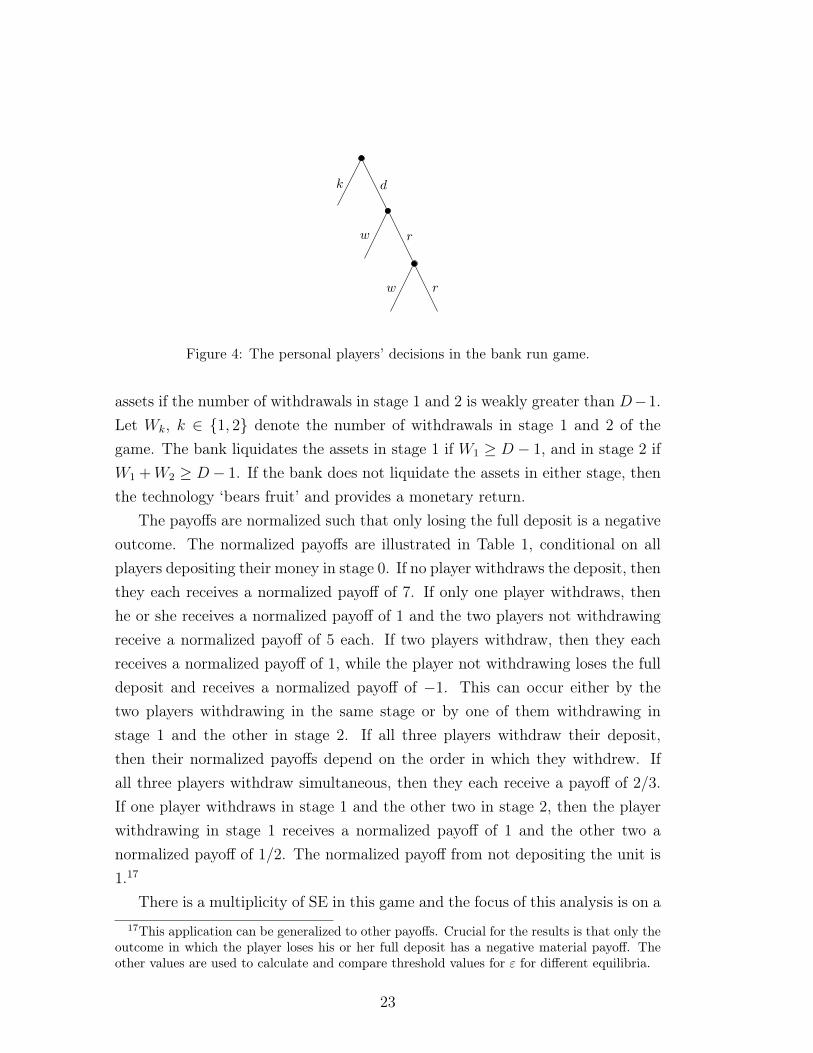
The game proceeds in three stages. In stage 0 the players have 1 monetaryunit and simultaneously decide whether to deposit it in the bank (d) or keep itin the mattress (k). Chance is passive in stage 0. In stage 1 and 2 of the game,all players with a deposit in the bank decide whether to withdraw it (w) or let itremain in the bank (r). The player’s decision tree is illustrated in Figure (4).
If a player decides to withdraw the deposit, then the deposit is withdrawnwith probability 1. In addition, the players face an exogenous risk of ‘needingmoney tomorrow’: in each stage each player faces the probability ε ∈ (0, 1) ofbeing selected by chance and forced to withdraw. I assume that the exogenousrisk of withdrawal is independent both between stages and between players.
Let D denote the number of players who deposited their money in the bank instage 0. After stage 0, the bank’s assets equals the units deposited by the players.If D > 1, then the bank invests in a technology for an immediate cost of 1. Thistechnology can provide a return after stage 2. The bank needs to liquidate the
22
k
w
w r
r
d
Figure 4: The personal players’ decisions in the bank run game.
assets if the number of withdrawals in stage 1 and 2 is weakly greater than D−1.Let Wk, k ∈ {1, 2} denote the number of withdrawals in stage 1 and 2 of thegame. The bank liquidates the assets in stage 1 if W1 ≥ D − 1, and in stage 2 ifW1 +W2 ≥ D− 1. If the bank does not liquidate the assets in either stage, thenthe technology ‘bears fruit’ and provides a monetary return.
The payoffs are normalized such that only losing the full deposit is a negativeoutcome. The normalized payoffs are illustrated in Table 1, conditional on allplayers depositing their money in stage 0. If no player withdraws the deposit, thenthey each receives a normalized payoff of 7. If only one player withdraws, thenhe or she receives a normalized payoff of 1 and the two players not withdrawingreceive a normalized payoff of 5 each. If two players withdraw, then they eachreceives a normalized payoff of 1, while the player not withdrawing loses the fulldeposit and receives a normalized payoff of −1. This can occur either by thetwo players withdrawing in the same stage or by one of them withdrawing instage 1 and the other in stage 2. If all three players withdraw their deposit,then their normalized payoffs depend on the order in which they withdrew. Ifall three players withdraw simultaneous, then they each receive a payoff of 2/3.If one player withdraws in stage 1 and the other two in stage 2, then the playerwithdrawing in stage 1 receives a normalized payoff of 1 and the other two anormalized payoff of 1/2. The normalized payoff from not depositing the unit is1.17
There is a multiplicity of SE in this game and the focus of this analysis is on a17This application can be generalized to other payoffs. Crucial for the results is that only the
outcome in which the player loses his or her full deposit has a negative material payoff. Theother values are used to calculate and compare threshold values for ε for different equilibria.
23

Table 1: Normalized material payoffs given that all players deposit their unit.
# Withdrawals πi(r) πi(w)
0 7 NA1 5 12 −1 13 NA 2/31, 2 NA 1, 1/2
‘good strategy profile’ in which all players plan to deposit their unit in the bankand not to withdraw in either stage.
Definition 3. The strategy profile σ is a good strategy profile if σi = (d, r, r) forall i ∈ I.
Players with standard preferences Consider the game between players withstandard preferences. If they use the good strategy profile, then player i’s initialexpected payoff is18
E [πi| (3, r) ;αi] =(2/3)ε3 + (1− ε)ε2 + (1− ε)2ε
+ 2(1− ε)2εE [πi| ((3, 1), r) ;αi]
+ (1− ε)3E [πi| ((3, 0), r) ;αi] .
(13)
When the players use the good strategy profile, they only withdraw their depositif forced to do so. The first term is the (exogenous) probability that all playerswithdraw in stage 1 for a normalized material payoff of (2/3). The second termis the probability that two players withdraw. If player i is one of them, then heor she receives a normalized material payoff of 1, otherwise he or she receives anormalized material payoff of −1. The third term is the probability that onlyplayer i withdraws in stage 1 for a normalized material payoff of 1. The fourthterm is the probability that a player j 6= i withdraws in stage 1 times the expectedmaterial payoff from stage 2. Likewise, the fifth term is the probability that noplayer withdraws in stage 1 times the expected material payoff from stage 2.
At the beginning of stage 2, the players observe the withdrawals in stage1. If two or more players withdrew, then a bank collapse has occurred and the
18With a slight abuse of notation, the history is written as the number of deposits in stage 0and the number of withdrawals observed after stage 1.
24

remaining player (if any) loses all of his or her money. If a player j 6= i withdrew,then player i’s expected payoff from not withdrawing in stage 2 is
E [πi| ((3, 1), r) ;αi] = 5(1− ε)2 + (1/2)ε2. (14)
If no player withdrew, then player i’s expected payoff from not withdrawing instage 2 is
E [πi| ((3, 0), r) ;αi] = (2/3)ε3 + (1− ε)ε2 + 11(1− ε)2ε+ 7(1− ε)3. (15)
The payoff from deviating and withdrawing the deposit is 1 in either stage. Forε < 0.496 the good strategy profile is an SE when the players have standardpreferences.
Players with two states of mind Now consider players who may transitionto the fearful state of mind. The maximin action in stages 1 and 2 is to withdrawthe deposit. Assume the players have identical fear thresholds, τi, and that theyuse the good strategy profile. In this case, peril is due to the exogenous risk ofwithdrawal.
Player i’s initial peril, the probability that the other two players will be forcedto withdraw, is
Pi(h0|αi
)= (1− ε)ε2 + 2(1− ε)3ε2 + (1− ε)4ε2. (16)
The first term is the probability that the other two players withdraw in stage1. The second term is the probability that one of the other players withdrawsin stage 1 and the other in stage 2. The third term is the probability that bothplayers withdraw in stage 2.
If no player withdrew in stage 1, then the updated peril is
Pi ((3, 0)|αi) = (1− ε)ε2. (17)
The updated peril corresponds to the probability that both other players areforced to withdraw in stage 2, but not player i.
The updated peril is smaller than the initial peril and P ′i ((3, 0)|αi) = 0. Thereis no increase in peril and the players do not transition to the fearful state of
25

mind. If at least 2 players withdrew in stage 1, then the bank has collapsed. Anyremaining player transitions to the fearful state of mind if sufficiently sensitiveto fear, but he or she has no action left to take and receives a payoff of −1.
The more interesting case is when only one player withdraws in stage 1. Theupdated peril for the remaining players is
Pi ((3, 1)|αi) = (1− ε)ε. (18)
The updated peril corresponds to the probability that (only) the other player isforced to withdraw in stage 2.
The increase in peril is
P ′i ((3, 1)|αi) = (1− ε)ε(1− (3(1− ε)3 + 1)ε). (19)
Let τ denote the maximum fear threshold for which the players transition tothe fearful state of mind conditional on observing one withdrawal in stage 1,τ = (1− ε)ε(1− (3(1− ε)3 + 1)ε). Once fearful, the players prefer to deviate tow. The plan of choosing r in both stages regardless the outcome of stage 1 cantherefore not be an optimal plan for such players.
Proposition 3. If the players are sufficiently sensitive to fear, τi ≤ τ , then thegood strategy profile cannot be an SE.
Fear sensitive bank run players may experience a welfare loss measured inmaterial payoffs. Moreover, this welfare loss is also imposed on their fear insensi-tive co-players. The social welfare maximizing strategy profile that fear sensitiveplayers can coordinate on is to not withdraw in stage 1 and withdraw in stage 2conditional on one player being forced to withdraw in stage 1. This strategy pro-file is an SE for ε ≤ 0.422. In this SE no player is fearful on the equilibrium path.The players coordinate on withdrawing conditional on observing one withdrawalin stage 1, and withdrawing is not a negative outcome. In addition, when theexogenous probability of withdrawal is sufficiently high, the game has a uniqueequilibrium in which all players chooses k and no money is invested. When theplayers may transition to the fearful state of mind, the exogenous probability forthis equilibrium to be unique is smaller than for players with standard prefer-ences. Since fear sensitive players cannot commit to r conditional on observinganother player withdrawing, they are less willing to choose d to begin with.
26

Fear can spread in a population of players with different fear thresholds. Con-sider the game between three players, but only i has τi ≤ (1 − ε)ε(1 − (3(1 −ε)3 + 1)ε. Assume the players use the good strategy profile, but that player j 6= i
is forced to withdraw in the first stage. This causes player i to transition tothe fearful state of mind. The third player, player k, knows the value of τi andcorrectly anticipates that player i will withdraw in the next stage. Consequently,his or her peril increases further and may reach τk, causing player k to transitionto the fearful state as well.
Proposition 4. A player with τi > τ may transition to the fearful state ofmind after observing one withdrawal in stage 1 if he or she knows that the otherremaining player will transition to the fearful state.
5 Public health intervention
As a final application, consider a simple example of a public health authority whowants to inform the public about accurate estimates of the probability or costof contracting a disease. This example stem from the observation that in manycases beliefs over the probability or cost of a negative outcome are mistaken.19
Consider a decision maker, player 1, who contemplates whether to take avaccine against a disease. Player 1 becomes immune to the disease if he or shetakes the vaccine. Otherwise player 1 faces a positive probability of contractingit.
Player 1 holds correct beliefs over the probability of contracting the diseaseand the cost of vaccination. However, he or she has underestimated the cost of thedisease.20 Recognizing this, the public health authority launches an informationcampaign to inform player 1 about the true cost. Note that the public healthauthority is not considered a player in this scenario.
The probability of contracting the disease (if not vaccinated) is denoted byε > 0, and the cost of vaccination is denoted by v, 0 < v < 1. Player 1’s priorbelief over the cost of the disease is denoted by d, and his or her updated beliefis denoted by d′, where d′ > d > 1.
19Or they may be correct but still possible to influence.20A related situation is the more ethically dubious case when the authority wants to scare
people into a certain behavior by overstating the cost.
27

The payoffs are normalized such that the only negative outcome is to con-tract the disease. The normalized payoff from not taking the vaccine and notcontracting the disease is 1. The normalized payoff from taking the vaccine is1− v. Finally, the normalized expected payoff of contracting the disease is 1− dand 1 − d′, when player 1 is uninformed and informed, respectively. Player 1’smaximin action is to take the vaccine.
First consider a player 1 who initially plans to take the vaccine. Player 1 isrisk neutral in the neutral state of mind and takes the vaccine if v ≤ εd. Becausethe only negative outcome is contracting the disease, player 1’s initial peril iszero, P1(h0;α1) = 0. He or she will take the vaccine and become immune to thedisease. The public health authority informs player 1 about the correct cost ofthe disease. However, since player 1 plans to take the vaccine, the updated perilis zero. There is no change in peril and, since v ≤ εd < εd′, player 1 is unaffectedby the information.
Next consider a player 1 who initially plans not to take the vaccine. That is,v ≥ εd. Player 1’s initial peril is
P1(h0;α1) = ε× d. (20)
The public health authority informs player 1 about the correct cost of the disease.As in traditional theory, player 1 changes his or her plan of taking the vaccine ifv ≤ εd′. In addition, a fear sensitive player may transition to the fearful state ofmind if the information causes a sufficiently large increase in peril.
Player 1’s increase in peril after receiving the information is
P ′1(info;α1) = ε(d′ − d). (21)
Player 1 transitions to the fearful state of mind if the increase in the cost of thedisease is sufficiently large such that τ1 is reached. In the fearful state of mind,player 1 maximizes minimum payoff by taking the vaccine also when v > εd′. Inother words, a fearful player 1 will take the vaccine also when the cost outweighthe benefits.
Proposition 5. Fear sensitivity can strengthen the behavioral response to infor-mation that increases the expected cost of negative outcomes.
As in traditional theory, if v ∈ (εd, εd′], then information alters behavior. A
28

player who remains in the neutral state of mind after receiving the informationtakes the vaccine also when εd < v ≤ εd′. However, a player who transitionsto the fearful state of mind after receiving the information takes the vaccineregardless the value of v. Fear sensitive players with a high cost of vaccinationmay overconsume the vaccine.21 On the other hand, vaccines often have a positiveexternality. Consider for example a disease which is highly transmissible, but theplayers fail to take the positive externality into account. In such a situation, afear response may increase social welfare.
6 Concluding Remarks
This paper presents a model of players who can transition from a neutral toa fearful state of mind. In the neutral state of mind, the players maximizeown expected material payoff. In the fearful state of mind, they maximize ownminimum material payoff. The players are in the neutral state of mind when thegame begins and transition to the fearful state after a sufficiently large increasein the expected cost of negative outcomes; outcomes bad enough to potentiallyinstill fear when anticipated.
The focus of this paper is on how fear affects behavior through its effect on aplayer’s risk aversion, but fear is also an unpleasant emotion. While the disutilityof experiencing fear is an incentive for players to avoid fearful situations, thispaper abstract from this to focus on how behavior is affected once a fearful stateis reached.
The interactions studied in this paper are assumed to be sufficiently fast suchthat there is no time to transition back to the neutral state of mind. However,many interactions are slower and allow for fear to fade away. Time can be ex-plicitly modeled using Psychological game theory (Battigalli et al., 2019) and themodel can be expanded to interactions which take place over several time peri-ods. The passing of a time period may cause a player to transition back to theneutral state of mind. Such a model requires an assumption regarding a fearfulplayer’s degree of sophistication which is not necessarily the same as the degreeof sophistication in the neutral state of mind.
21The cost of vaccination may for example include expected side effects that may vary betweenplayers with different health statuses.
29

The transition from the neutral to the fearful state of mind is determinedby beliefs over outcomes. This definition rules transitions caused by a player’sbeliefs over others’ beliefs. For example, someone might become fearful if he orshe believes that their boss believes that he or she has low productivity. However,one can model this situation as a player with the negative outcome of losing hisor her job. An increase in the belief that the boss believes that he or she has lowproductivity causes an increase in the probability that he or she will lose the job,which may trigger fear.
Players’ increased concern with risk in the fearful state of mind causes anstrengthened change in behavior that may appear as an overreaction. This ob-servation is in line with empirical and experimental research that finds a ’residual’change in behavior after bad news or adverse events (Guerrero et al., 2012; Guisoet al., 2018; Piccoli et al., 2017; Wang & Young, 2020). In other words, the be-havioral response is stronger than what can be explained by traditional factorsalone. The residual change in behavior is however consistent with an emotion-based change of the utility function.
This paper studies sophisticated players who can perfectly predict own andothers’ state transitions and the behavioral consequences thereof. In the sequen-tial equilibrium for psychological games, the players are certain about own andothers’ plans, and never change their minds about them. Any deviations fromthe plans are interpreted as mistakes. This is a strong assumption, especiallysince the players’ decision utility may depend on both own and others’ plans.However, the analysis shows that fear is of importance even when players canperfectly predict own and others’ state transitions. Whereas the study of naïveplayers who cannot perfectly predict own emotional response is outside the scopeof this paper, it is an interesting avenue for future research.
It is natural to ask whether fear, modeled as belief-dependent risk aversion,makes sense from an evolutionary perspective. Aumann (2019) argues that peopleuse rules to guide their behavior and that these behavioral rules are the productof evolutionary forces. Rather than maximizing utility over actions, people adoptrules of behavior that do well in usual, naturally occurring situations. A simpleexample of such a rule related to fear could be ‘maximize expected utility whenin a safe environment while minimize the worst losses when in peril’.
Besides robberies, bank runs, and public health policy, fear may be impor-
30

tant in understanding for example conflict; environmental dangers and climaterisk; and financial decision making. These applications are potentially of greatimportance and are left as an avenue for future research.
31

References
Alempaki, D., Starmer, C., & Tufano, F. (2019). On the priming of risk prefer-ences: The role of fear and general affect. Journal of Economic Psychology, 75,102-137.
Andrade, E. B., & Ariely, D. (2009). The enduring impact of transient emotionson decision making. Organizational Behavior and Human Decision Processes,109(1), 1-8.
Attanasi, G., Battigalli, P., & Manzoni, E. (2016). Incomplete-information modelsof guilt aversion in the trust game. Management Science, 62(3), 648-667.
Aumann, R. J. (2019). A synthesis of behavioural and mainstream economics.Nature Human Behaviour, 3(7), 666-670.
Battigalli, P., Corrao, R., & Dufwenberg, M. (2019). Incorporating belief-dependent motivation in games. Journal of Economic Behavior & Organization,167, 185-218.
Battigalli, P., & Dufwenberg, M. (2007). Guilt in games. American EconomicReview, 97(2), 170-176.
Battigalli, P., & Dufwenberg, M. (2009). Dynamic psychological games. Journalof Economic Theory, 144(1), 1-35.
Battigalli, P., & Dufwenberg, M. (2020). Belief-Dependent Motivations and Psy-chological Game Theory. Forthcoming in Journal of Economic Literature.
Battigalli, P., Dufwenberg, M., & Smith, A. (2019). Frustration, aggression, andanger in leader-follower games. Games and Economic Behavior, 117, 15-39.
Bernheim, B. D., & Rangel, A. (2004). Addiction and cue-triggered decisionprocesses. American economic review, 94(5), 1558-1590.
Bernheim, B. D., & Rangel, A. (2009). Beyond revealed preference: choice-theoretic foundations for behavioral welfare economics. The Quarterly Journalof Economics, 124(1), 51-104.
32

Callen, M., Isaqzadeh, M., Long, J. D., & Sprenger, C. (2014). Violence andrisk preference: Experimental evidence from Afghanistan. American EconomicReview, 104(1), 123-48.
Campos-Vazquez, R. M., & Cuilty, E. (2014). The role of emotions on risk aver-sion: a prospect theory experiment. Journal of Behavioral and ExperimentalEconomics, 50, 1-9.
Caplin, A., & Leahy, J. (2001). Psychological expected utility theory and antici-patory feelings. The Quarterly Journal of Economics, 116(1), 55-79.
Cohn, A., Engelmann, J., Fehr, E., & Maréchal, M. A. (2015). Evidence for coun-tercyclical risk aversion: An experiment with financial professionals. AmericanEconomic Review, 105(2), 860-85.
Diamond, D. W., & Dybvig, P. H. (1983). Bank runs, deposit insurance, andliquidity. Journal of Political Economy, 91(3), 401-419.
Dijk, O. (2017). Bank run psychology. Journal of Economic Behavior & Organi-zation, 144, 87-96.
Dillenberger, D., & Rozen, K. (2015). History-dependent risk attitude. Journalof Economic Theory, 157, 445-477.
Frederick, S., & Loewenstein, G. (1999). Hedonic adaptation: In D. Kahneman,E. Diener, N. Schwarz (eds), Well-Being. The foundations of Hedonic Psychol-ogy New York: Russell Sage Foundation Press, 302-329.
Frijda, N. H. (1986). The emotions. Cambridge: Cambridge University Press.
Fudenberg, D., & Levine, D. (1986). Limit games and limit equilibria. Journal ofeconomic Theory, 38(2), 261-279.
Garratt, R., & Keister, T. (2009). Bank runs as coordination failures: An exper-imental study. Journal of Economic Behavior & Organization, 71(2), 300-317.
Gärtner, M., Mollerstrom, J., & Seim, D. (2017). Individual risk preferences andthe demand for redistribution. Journal of Public Economics, 153, 49-55.
33

Geer, J. H. (1965). The development of a scale to measure fear. Behaviour Re-search and Therapy, 3(1), 45-53.
Guerrero, F. L., Stone, G. R., & Sundali, J. A. (2012). Fear in Asset AllocationDuring and After Stock Market Crashes An Experiment in Behavioral Finance.Finance & Economics, 2(1), 50-81.
Guiso, L., Sapienza, P., & Zingales, L. (2018). Time varying risk aversion. Journalof Financial Economics, 128(3), 403-421.
Holtgrave, D. R., & Weber, E. U. (1993). Dimensions of risk perception for fi-nancial and health risks. Risk Analysis, 13(5), 553-558.
Jackson, M. O., Rodriguez-Barraquer, T., & Tan, X. (2012). Epsilon-equilibriaof perturbed games. Games and Economic Behavior, 75(1), 198-216.
Kahneman, D. & Tversky, A. (1979). Prospect Theory: An Analysis of DecisionUnder Risk. Econometrica 47(2), 263-291
Kőszegi, B., & Rabin, M. (2007). Reference-dependent risk attitudes. AmericanEconomic Review, 97(4), 1047-1073.
Kreps, D. M., & Wilson, R. (1982). Sequential equilibria. Econometrica, 863-894.
Kuhnen, C. M., & Knutson, B. (2011). The influence of affect on beliefs, prefer-ences, and financial decisions. Journal of Financial and Quantitative Analysis,46(3), 605-626.
LeDoux, J. (1998). The emotional brain: The mysterious underpinnings of emo-tional life. New York: Simon and Schuster.
Lerner, J. S., Gonzalez, R. M., Small, D. A., & Fischhoff, B. (2003). Effects offear and anger on perceived risks of terrorism: A national field experiment.Psychological Science, 14(2), 144-150.
Lerner, J. S., & Keltner, D. (2000). Beyond valence: Toward a model of emotion-specific influences on judgement and choice. Cognition & Emotion, 14(4), 473-493.
34

Lerner, J. S., & Keltner, D. (2001). Fear, anger, and risk. Journal of Personalityand Social Psychology, 81(1), 146-159.
Malmendier, U., & Nagel, S. (2011). Depression babies: do macroeconomic expe-riences affect risk taking?. The Quarterly Journal of Economics, 126(1), 373-416.
Loewenstein, G. F., Weber, E. U., Hsee, C. K., & Welch, N. (2001). Risk asfeelings. Psychological bulletin, 127(2), 267-286.
Monderer, D., & Samet, D. (1989). Approximating common knowledge with com-mon beliefs. Games and Economic Behavior, 1(2), 170-190.
Nguyen, Y., & Noussair, C. N. (2014). Risk aversion and emotions. Pacific Eco-nomic Review, 19(3), 296-312.
Piccoli, P., Chaudhury, M., Souza, A., & da Silva, W. V. (2017). Stock overre-action to extreme market events. The North American Journal of Economicsand Finance, 41, 97-111.
Radner, R. (1980). Collusive behavior in noncooperative epsilon-equilibria ofoligopolies with long but finite lives. Journal of Economic Theory, 22(2), 136-154.
Schelling, T. C. (1980). The Strategy of Conflict. Cambridge: Harvard UniversityPress.
Smith, C. A., & Ellsworth, P. C. (1985). Patterns of cognitive appraisal in emo-tion. Journal of Personality and Social Psychology, 48(4), 813-838.
Smith, C. A., & Lazarus, R. S. (1991). Emotion and adaptation. Oxford: OxfordUniversity Press.
Thaler, R. H., & Shefrin, H. M. (1981). An economic theory of self-control. Jour-nal of political Economy, 89(2), 392-406.
O’Donoghue, T., & Rabin, M. (2001). Choice and procrastination. The QuarterlyJournal of Economics, 116(1), 121-160.
35

Wang, A. Y., & Young, M. (2020). Terrorist attacks and investor risk preference:Evidence from mutual fund flows. Journal of Financial Economics, 137(2), 491-514.
36