fault trace complexity, cumulative slip, and the shape of the

Geophys. J. Int. (1996) 124, 833-868

Fault trace complexity, cumulative slip, and the shape of the magnitude-frequency distribution for strike-slip faults: a global survey

Mark W. Stirling,'." Steven G. Wesnousky' and Kunihiko Shimazaki2 ' Centerfor Neotectonic Studies and Department of Geological Sciences, University of Nevada, Reno, NV 89557, USA 'Earthquake Research Institute, University of Tokyo, Yayoi 1-1-1, Bunkyo-ku, Tokyo 113, Japan

Accepted 1995 October 7. Received 1995 September 1; in original form 1995 March 23

SUMMARY We examine whether the shape of the magnitude-frequency distribution for strike-slip faults is described by the Gutenburg-Richter relationship (log n = a - b M ) or by the characteristic earthquake model, by analysing a data set of faults from California, Mexico, Japan, New Zealand, China and Turkey. For faults within regional seismic networks, curves of the form log n y r p l = a - bM, where n yr-' is the number of events per year equal to magnitude M , are fit to the instrumental record of seismicity, and geological data are used to estimate independently the size and recurrence rate of the largest expected earthquakes that would rupture the total length of the fault. Extrapolation of instrumentally derived curves to larger magnitudes agrees with geological estimates of the recurrence rate of the largest earthquakes for only four of the 22 faults if uncertainties in curve slope are considered, and significantly underesti- mates the geological recurrence rates in the remaining cases. Also, if we predict the seismicity of the faults as a function of fault length and slip rate, and the predicted seismicity is distributed in accord with the Gutenburg-Richter relationship, we find the predicted recurrence rate to be greater than the observed recurrence rates of smaller earthquakes along most faults. If individual fault zones satisfy the Gutenburg-Richter relationship over the long term, our observations imply that, during the recurrence interval of the largest expected earthquakes, the recurrence of lesser-sized events is not steady but, rather, strongly clustered in time. However, if the instrumental records provide an estimate of the long-term rate of small to moderate earthquakes along the faults, our observations imply that the faults generally exhibit a magnitude-frequency distribution consistent with the characteristic earthquake model. Also, we observe that the geometrical complexity of strike-slip faults is a decreasing function of cumulative strike-slip offset. The four faults we observe to be consistent with the Gutenburg- Richter relationship are among those characterized by the least amount of cumulative slip and greatest fault-trace complexity. We therefore suggest that the ratio of the recurrence rate of small to large earthquakes along a fault zone may decrease as slip accumulates and the fault becomes smoother.

Key words: b values, earthquakes, fault slip, strike slip.

from earlier work of Wesnousky (1988), which suggested, on the basis of a small data set of faults primarily from California, that fault trace complexity decreases as a function of cumulative offset. The motivation for ( 2 ) stems from the question of whether or not seismicity along a single fault is described by the Gutenburg-Richter relationship

log = a - b M ,

where n is the number of events of magnitude M , and a and b

INTRODUCTION

We use a global data set of strike-slip faults to examine whether or not (1) the geometrical complexity of fault traces or (2) the shape of the magnitude-frequency distribution along particular faults is a function of the amount of cumulative strike-slip offset recorded by the faults. The motivation for (1) arises

* Email: [email protected]

(1)

0 1996 RAS 833

Dow

nloaded from https://academ

ic.oup.com/gji/article/124/3/833/584043 by guest on 30 January 2022

834 M . W. Stirling, S. G. Wesnousky and K . Shimazaki

are empirical constants (Ishimoto & Iida 1939; Gutenburg & Richter 1944). Catalogues of regional seismicity are typically well described by the Gutenburg-Richter relationship (eq. 1). The assumption that seismicity on a single fault also satisfies eq. (1) implies that there will be numerous lesser-sized events in the time interval between the occurrence of the largest earthquakes on a fault (Fig. la). However, a number of studies have reported evidence to suggest that seismicity along faults does not satisfy eq. (1) across the entire magnitude range, but instead shows a greater frequency of occurrence of large earthquakes than would be expected from extrapolation of curves fit to the log-linear distribution of lesser-sized earthquakes (Wesnousky et al. 1983; Schwartz & Coppersmith 1984; Youngs & Coppersmith 1985; Wesnousky 1994), the concept now commonly referred to as the characteristic earthquake model of fault behaviour (Fig. lb). Determining whether it is the Gutenburg-Richter relationship or the characteristic earthquake model that describes the seismicity along particular faults is problematic because historical records of seismicity are generally much shorter than the repeat time of the largest earthquake on a fault. However, the recurrence of the largest- sized events along a fault can be estimated independently with geologicalIy determined palaeoearthquake histories and fault slip-rate data. Thus, in addition to examining the geometrical complexity of strike-slip faults, we combine instrumental records of seismicity with interpretation of palaeoearthquake and fault slip-rate data to examine the shape of the magnitude- frequency distribution for the global data set of strike-slip faults.

(a) Gutenburg - Richter Relationship A A

(b) Characteristic Earthquake Model

Ma Mmax Ma Mmm

Figure 1. Schematic illustration of the discrete and cumulative forms of the magnitude-frequency distributions for the faults described by (a) the Gutenburg-Richter relationship and (b) the characteristic earthquake model of fault behaviour during the repeat time of one maximum magnitude (Mmax) event along a fault. The discrete number of events of a given magnitude per year is represented by n, and N is the cumulative number of events greater than or equal to a given magnitude. For the characteristic earthquake model, the largest earthquake during the repeat time of a maximum magnitude event is defined to equal the size of the largest aftershock (Ma) and the size distribution of aftershocks is assumed to satisfy the Gutenburg- Richter model.

DATA A N D ANALYSIS

Our analysis is limited to strike-slip faults that are (1) located within regional seismic networks, (2) have been the focus of fault slip-rate or palaeoearthquake studies, or (3) for which maps of sufficient detail exist to define discontinuities in fault trace that measure a kilometre or greater in width normal to fault strike. The faults considered are located in California, Mexico, New Zealand, Japan, China and Turkey. For con- venience of presentation, the maps and a brief discussion of data bearing on the cumulative strike-slip offset and slip rate of each fault are given in Appendix A. The location and size of steps in fault trace, measuring 1 km or more in width perpendicular to fault strike, are marked on the strip maps for each fault in Fig. A1 of the Appendix. Following the approach of Wesnousky (19881, we define the complexity of a fault trace as the number of observed steps per unit length of fault trace. Table 1 summarizes the data and references describing the length, cumulative strike-slip offset, slip rate and fault-trace complexity for each fault. When uncertainty exists in defining the number of steps along a fault trace, a range of values is listed for the number of steps and, hence, fault-trace complexity. The smaller values of complexity reflect the number of clearly defined steps, and the larger values reflect the sum of both clearly defined and possible steps. Included as 'possible steps' in some cases are those steps located very close to the ends of faults that may be part of a fault splay or termination. The value of fault-trace complexity is plotted versus cumulative strike-slip offset in Fig. 2. We defer discussion of the plot to the Discussion section of the paper.

It is only the faults listed in Table 2 and located in California, Japan, New Zealand, and Baja California that fall within regional seismic networks that have been recording for a relatively long period of time. The faults of southern California fall within the CIT-USGS network, which has been recording since 1932 (Given, Hutton & Jones 1987). The epicentral distribution of seismicity for events of M 2 3 for the period 1932-92 is shown in Fig. 3(a) within a polygon encompassing all of the southern California faults listed in Table 2. The faults of northern California are within the USGS-CALNET seismic network, which has been officially recording since 1969. The epicentral distribution of seismicity for events of M 2 3 for the period 1969-92 is shown in Fig. 3(a) for a region encompassing the northern California faults listed in Table 2. The San Miguel-Vallecitos fault is the only fault zone considered in Baja California, Mexico. The RESNOR seismic network of northwestern Baja California has been in operation since 1976 (Vidal & Munguia 1993). We show the polygon that encompasses northwestern Baja California in Fig. 3(a). Seismicity in the vicinity of the Japanese faults has been recorded by the Japanese Meteorological Agency network since 1926 (Ichikawa 1969; Mochizuki, Kobayashi & Kishio 1978; Yokoyama 1984). The epicentral distribution of M 2 3 events in the vicinity of the Japanese faults listed in Table 2 is shown for the period 1926-92 in Fig. 3(b). The Institute of Geological and Nuclear Sciences (formerly DSIR) has been operating a computerized seismic network in New Zealand since 1964 (Smith 1976). The epicentral distribution of M 2 3 events in the area of the New Zealand faults listed in Table 2 is shown in Fig. 3(c) for the period 1964-92. All the epicentral distributions represented in Fig. 3 are limited to events with depths <20 km. Slightly different methods are used in each

0 1996 RAS, G J I 124, 833-868

Dow



Magnitude distribution of strike-slip faults 835

Table 1. Geological data. Note that LL = left-lateral strike-slip offset, RL = right-lateral strike-slip offset, 0s = fault with oblique-slip motion. Slip rates are shown for the faults that form the data set in Table 2, and published preferred slip rates are given in parentheses; see Appendix. The minimum step number represents the number of clearly defined steps, and the maximum number represents the total of clearly defined and possible steps. Fault length, cumulative offset and slip rate data sources are as follows: (1) Crowell (1962); Grantz & Dickenson (1968); Hill (1981); Petersen & Wesnousky (1994); (2) Smith (1962); Petersen & Wesnousky (1994); (3) Barrows (1974); Petersen & Wesnousky (1994); (4) Hull & Nicholson (1992); Petersen & Wesnousky (1994); (5) Rockwell et a(. (1990); Petersen & Wesnousky (1994); (6-10) Dokka (1983); (11) Gastil et al. (1975); Harvey (1985); Hirabayashi et al. (1993); [ 12) Prentice et al. (1993); Working Group on California Earthquake Probabilities (1990); (13) Kintzer et al. (1977); Matsu’ura et al. (1986); Galehouse (1991); (14) Budding et al. (1991); Lienkaemper et al. (1991); (15) Okada (1980); Research Group for Active Faults of Japan (1992); (16-19) Okada & Ikeda (1991); Research Group for Active Faults of Japan (1992); (20) Research Group for Active Faults of Japan (1992); (21) Wellman (1953); Hull & Berryman (1986); Berryman & Beanland (1988); (22) Wellman (1953); Berryman & Beanland (1988); (23) Lensen (1960); Knuepfer (1992); (24) Browne (1992); (25) Freund (1971); Cowan (1990, 1991); Cowan & McGlone (1991); Van Dissen & Yeats (1991); (26) Wellman (1972); Berryman & Beanland (1988); (27) Berryman & Beanland (1988); Van Dissen et al. (1992); Institute of Geological and Nuclear Sciences (1994); (28) Institute of Geology (1991); (29) Institute of Geology (1990); (30) Barka & Gulen (1988).

ID & FAULT LENGTH STRIKE SLIP OFFSET SLIP KATE NO OF STEPS COMPLEXITY (km) (km) ( m m h ) ( s t e p h )

Southern Cnlifornin 1 San Andreas

Bitterwater 2 Garlock 3 Newport-Inglewocd 4 Whittier-Elsinore 5 San Jacinto Mojnve Desert 6 Calico-Mesquite 7 Pisgah 8 Camprock 9 Helendale 10 Lenwood

(total length) 1000 - Salton Sea 550

240 60 240 2x)

125 64 73-93 58-80 75

- >I50 2150 64 0.2-10 10-15 24

8.2 6.4- 14.4 1.6-4 3 1.5-3

1-43 RL 1 11-43(24)RL 1 4-9 LL 1 0.1-6(0.6) RL 4 1.5-9.3(5) RL 3 7- 19(12)RL 5

3-4 2 1-3 3 1-2

,001 ,0018 ,0042 ,066 ,0125 ,022

,024-,032 ,031 ,011-,041 ,038-,052 ,013-,014

Bnjn Cnlifornin 11 San Miguel-Vallecitos 160 0.5 0.1-0.5 RL 4-6 ,025-,038

Northern California 12 San Andreas (Mendocino-San Juan Bautista) 460 2150 1-32 RL 0 0 13 Calaveras-Concord-Green Valley-Bartlett Sp 220 24 3-25(8) RL 5-7 ,023-,032 14 Hayward-Rogers Creek-Maacama 250 2.1-9(9) RL 2-3 ,008-.012

Japan 15 MTL (Shikoh Island) 16 Neodani 17 Atrra 18 Atotsugawa 19 Tanna 20 Yarnasaki

215 100 60 60 30 80

5 3-5 7-10 3 1

,014-.023 1-2(2) LL 2-3 .02-.03 3-5.2(5.2) LL 1-2 ,017-,033 1-5 RL 2-3 .03-.05 1-2(2) LL 2-3 .067-. 1 0.3-0.8 LL 0-2 0-,025

7-8(7) RL 3-5

New Zevlrnd 21 Alpine (onland extent. 0s) 22 Wairau 23 Awatrre 24 Clarence 25 Hope 26 Wairarapa (0s) 27 Wellington

520 100 170 1 80 220 180 200

480 430-480 19 15 19

10-12

25-4s RL 3.8-6 RL 0- 1 0-,013 5-10 RL 4-8 RL 11-25 RL 1-3 ,0045-.014

5-7.6(7.1) RL 1-2 ,005-.01 8-12.3(8) RL 3-6 .033-,167

China 28 Altun 29 Haiyuan

1600 280

65-75 12-14.5

2-7 .0012S-,00375 2-4 , oO714-.0143

Turkey 30 N. Analolian 980 25-45 12 ,012

network to estimate magnitude, but the various scales (local paper to define the size of the largest earthquakes on all of magnitude, ML, in southern California and New Zealand; coda the faults. magnitude, Mc, in northern California and Baja California; For each of the regions enclosed by polygons in Figs 3(a) and the Japanese Meteorological Agency magnitude, M,,,, in (northern and southern California, and Baja California), Japan) generally correlate with moment magnitude (Given 3(b) (Japan) and 3(c) (New Zealand), the number of events et al. 1987; Smith 1976; Lee, Bennett & Meagher 1972; Utsu per year is plotted as a function of magnitude in Fig. 4 1982; Hanks & Kanamori 1979), which we use later in the (magnitudefrequency distributions). Also shown in Fig. 4 are

0 1996 RAS, GJI 124, 833-868

Dow



836 M. W. Stirling, S . G. Wesnousky and K . Shimazaki

0.1

0.001

0.1

I I I J I I

+

1

19

8 &

m r-

southern California /BajaCalif A northern California 27

Y v1

Japan

New Zealand u China

1 6 3

N N

I I I I i

A Turkey

1 10 I00 Strike slip offset (km)

Figure 2. Graph of fault-trace complexity versus cumulative strike-slip offset for faults listed in Table 1. The identification numbers of the faults (Table 1) are also shown. Error bars reflect uncertainties in the definition of fault steps and in the amount of cumulative strike-slip offset.

histograms of the number of events per year for each region. The magnitude-frequency curves are approximately of linear slope over the range of highest magnitudes for each region, and show a decrease to smaller slopes at smaller magnitudes. For the purpose of this analysis we attribute the decrease in slope at smaller magnitudes to the magnitude detection threshold for each region. We note that value by a vertical dotted line in each plot of Fig.4 and only consider seismicity of magnitude greater than the detection threshold in the ensuing analysis. Analysis of the distributions is therefore limited to M 2 3 for the southern California region, M 2 2 for the northern California region, M 2 3 for the northwest Baja California area, M 2 4 . 5 for central Japan, and M 2 4 for central New Zealand (Fig. 4). We also limit our attention to the period 1944-92 in the case of the CIT-USGS data because magnitudes were only reported to the nearest 0.5 magnitude unit prior to that time. Each magnitude-frequency distribution is described by a set of lines in the form of eq. (1). The value of b is fit by the maximum likelihood method (Utsa 1965; Aki 1965), and is shown for each region in Fig. 4. The value of a is fit to satisfy the total number of events greater than the detection threshold magnitude obtained in Fig. 4. For each region, the three diagonal dotted lines represent the maximum- likelihood fit to the data and the 95 per cent confidence limits for that fit, and thus define the regional b value. The number N of events used in determining the b value, the estimated b value and 95 per cent confidence limits, and the instrumental seismic moment rate &fo(instr) is also listed in the top right corner of each plot. &f, (instr) is the sum of the seismic moments of all recorded events of magnitude greater than the detection threshold magnitude divided by the number of years of recording, where the seismic moment of each event is

determined from the magnitude by use of the relationship log M , = 1.5M + 16.1 (Hanks & Kanamori 1979).

To characterize the magnitude-frequency distribution for individual faults, we consider only seismicity recorded within polygons encompassing each of the faults in Table2. The polygons for faults in California, Baja California, Japan and New Zealand are shown in Fig. 5. The polygons generally include seismicity within approximately 20 km of the respective faults, except in cases where neighbouring active faults are closer then 20 km, in which case the width is reduced. The character of seismicity for each fault is depicted by the plots in Figs 6 and 7. Fig. 6 shows the discrete number of events per year versus magnitude and Fig. 7 shows a histogram of the number of events per year determined from the seismicity recorded in the respective polygons. The histograms serve to show any temporal variations in seismicity rates. The open circles in the magnitude-frequency plots for each fault (Fig. 6) represent the instrumental record of seismicity. The plots do not show events of magnitudes less than the detection threshold magnitudes for each region, except in the case of Japan where seismicity down to M4 is shown. The recorded seismicity at M4 is assumed on the basis of Fig. 4 to closely approximate actual seismicity in central Japan. Lines of the form of eq. (1) are fit to the instrumental record of seismicity (open circles) for each fault by use of the maximum-likelihood method. The maximum-likelihood fit to the instrumental record and 95 per cent confidence limits are also shown as a set of three heavy dotted lines, which, for clarity, are only plotted at magnitudes greater than 5. We have not attempted to fit lines of the form of eq. (1) to the Hope, Wairau, Wairarapa, Wellington and Japanese faults, because each of these areas records fewer than 10 events with magnitudes greater than the detection threshold

0 1996 RAS, GJI 124, 833-868

Dow




Table 2. Maximum magnitudes and return times calculated from the geological data in Table 1, assuming rupture of the entire lengths of the faults listed. Calculations are limited to those major faults that fall within the remit of the CIT-USGS (southern California), USGS- CALNET (northern California), RESNOR (northwest Baja California), Japanese Meteorological Agency (central Japan) and Institute of Geological and Nuclear Sciences (New Zealand).

ID & FAULT MAXIMUM RETURN MAGNITUDE* TIME (yrs)**

pref rnin max pref Tminl TminZ Tmaxl Tmax2

( M: preO( M: min)( M: max)

Southern California

Salton Sea) 2 Garlock 7.5 7.3 7.7 393 131 294 1184 526

3 Newport-Inglewood 7.0 6.8 7.2 2941 1 39 8348 52353 873

4 Whittier-Elsinore 7.5 7.3 7.7 468 126 781 3171 511

5 San Jacintp: 7.6 7.3 7.7 663 169 253 1678 1119

Baja California 11 San Miguel- 7.4 7.2 7.6 11835 3023 7557 45280 18112 Vallecitos

1 San Andreas (Bitkrwater- 7.9 7.7 11.1 146 39 154 799 204

Northern California 12 San Andreas Mendocino - San Juan Bautista) 13 Calaveras-Concord- Green V-Bartlett Sp 14 Hayward-Rogers Ck-Maacama

7.11 7.6 8.0 154 46 209 928 203

7.5 7.4 7.7 318 61 506 1715 206

646 2734 638 7.6 7.4 7.8 281 151

Japan 15 MTL

16 Neodani

17 Atera

18 Atotsugawa

19 Tanna

20 Yamsaki

7.9 7.5 8.3 1188 285 326 4753 4159

7.5 7.1 7.9 2149 667 1334 18428 9214

7.2 6.8 7.6 573 164 285 3494 2015

7.2 6.8 7.6 1195 171 855 10607 2121

6.8 6.5 7.2 900 270 540 8944 4472

7.5 7.1 7.9 22016 3036 8097 559440 209790

New Zealand 21 Alpine 7.8 7.6 8.1 79 33 60 310 172

22 Wairau 7.2 6.9 7.4 405 116 183 101 1 640

23 Awatere 7.4 6.6 7.7 340 12 24 1184 592

24 Clarence 7.4 7.2 7.6 309 123 247 928 464

25 Hope 7.5 7.4 7.7 140 60 137 459 202

26 Wairarapa 7.4 7.2 7.6 231 80 123 463 MI

27 Wellington 7.5 7.2 7.6 313 124 189 778 512

* Magnitudes are calculated by use of the equation log M , = 16.1 + 1.5M. **Return times T are calculated from equations 4 and 5(a)-(d) in the text. Negative values for T result from &f;'" > ME, the case for the extreme low bounds on & f E for the northern San Andreas and Tanna faults. &f:m is therefore based on records from which the mainshock of the Loma Prieta earthquake is removed in the case of the northern San Andreas fault, and the 1930 mainshock removed in the case of the Tanna fault.

magnitude. With the assumption that the magnitude-frequency distributions remain linear at magnitudes greater than those recorded during the instrumental recording period, the heavy dotted lines may be used to place bounds on the expected rate of occurrence of the largest expected earthquakes along the fault zones. Also plotted in the magnitude-frequency plots for each fault are a set of open and closed diamonds. The diamonds represent bounds on the size and recurrence rate of the

maximum expected earthquake along each fault zone arising from interpretation of geological observations. Determination of the values is described in the following paragraphs.

Estimation of the maximum expected earthquake size along mapped faults commonly arises from measures of fault length. For the purposes of this analysis, we assume that each of the faults is capable of rupturing along the entire fault length during a single earthquake. The seismic moment that would

0 1996 RAS, GJI 124, 833-868

Dow



838 M . W Stirling, S. G. Wesnousky and K. Shimazaki

(4

Seismicitv from CALNET-USGS hl

I here) I

Figure 3. Instrumental seismicity for M 2 3 and depth 5 2 0 km plotted on a map of major faults for (a) California and northern Baja California over the time periods 1932-92 (southern California and Baja California) and 1969-92 (northern California), (b) central Japan over the time period 1926-92, and (c) central New Zealand over the time period 1964-92. The boxes on each map represent the search areas used to extract data from the respective seismicity catalogues. We show the box used to extract seismicity from the RESNOR network of Baja California, but, as the diagram is for illustrative purposes only, we have simplified the plotting procedure by showing seismicity from the CIT-USGS catalogue over the area.

0 1996 RAS, GJI 124, 833-868

Dow




Figure 3. (Continued.)

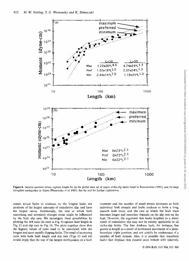
be associated with rupture of the entire fault length can be estimated from empirical measurements of seismic moment versus fault length for instrumentally recorded earthquakes in interplate (Fig. 8a) and Japanese intraplate (Fig. 8b) environments. The interplate and Japanese intraplate data sets are taken from the compilations of Romanowicz (1992) and Wesnousky et al. (1983), respectively. Lines of the form M : = C,Ld are fit to the data sets, where Mz is the expected seismic moment, L is earthquake rupture length, and C, and d are empirically derived constants. The curve fits labelled ‘preferred‘, ‘minimum’ and ‘maximum’ provide us with the empirical basis to estimate the preferred (Mzpref ), minimum (Mzmin) and maximum (Mzmax) bounds on the seismic moment for an earthquake rupturing the entire length of each fault listed in Table 2. The seismic moments ( M z ) of earthquakes, assuming a complete rupture of each fault, are con- verted to moment magnitude and listed for each fault in Table 2.

We may further estimate the recurrence interval T of maximum expected events along each fault zone in Table2 by dividing the cumulative seismic moment release Z M , expected during the recurrence interval T by a geologically determined average seismic moment rate &ff for the fault,

where M z is the seismic moment of the maximum expected event and Z Mim is the sum of seismic moment release of events with M , < Mz that will contribute to fault slip during the recurrence interval T. Eq. (2) can be rewritten as follows:

T = (M:/M:)/[ 1 - (M:m/&f:)], (3) whereby Mim is approximated by the empirically determined instrumental moment release rate &f,(instr), which is listed

for each fault in the lower left of each plot in Fig. 6. Seismic moment M , is defined to equal pLWU (Aki & Richards 1980), where p is the shear modulus (assumed to equal 3 x 10” dyne cm-2), L, the fault length, W, the fault width (approximated to 15 km for all faults), and U, the coseismic slip. Substituting geologically determined fault slip rate US for coseismic slip U, we can define the rate of seismic moment release Mf = pLWUg (e.g. Brune 1968), using the same values of p and Was above. The fault maps we have used to estimate fault lengths L and a discussion of the geological data bearing on the slip rate U g for each of the faults listed in Table 1 are provided in Appendix A. The minimum, maximum and preferred values of slip rate are further summarized in Table 1, along with values of fault length L. The data provide the basis to define the preferred hjf(pref), maximum il&max), and minimum Mf(min) values of seismic-moment release rate for each fault. &ff(min) and hif(max) are shown at the bottom of each plot in Fig. 6 [M,(geol)]. Recalling that minimum, maximum and preferred values of Mz may be determined from empirical relationships in Fig. 8, we use eq. (3) to place bounds on the recurrence interval T for the largest expected earthquakes along the fault zones. More specifically, the preferred estimate of return time is defined as

Tpref= [~~(pref)/&f:(pref)]/{l- [&fim/Mnif(pref)l } , (4) and maximum (Tmax) and minimum (Tmin) bounds on recurrence interval are calculated as

Tminl= [~z(min) /Mf(max) l /{~ - [~2:~/&fhif(max)l} , (5a)

Tmin2 = [Mz(min)/&fhif(min)]/{ 1 - [~~m/&ff (max) ]} , (5b)

Tmaxl = [Mz(max)/M$(min)]/{ 1 - [&fim/&ff(min)]}, (5c)

Tmax2 = [Mz(max)/Mt(max)]/{ 1 - [&f:rn/M$(min)] } . (5d)

0 1996 RAS, GJI 124, 833-868

Dow



840 M . W. Stirling, S . G. Wesnousky and K . Shimazaki

SOUTHERN CALIFORNIA

instr)=4.77e+25 dyne-cdyr

2 3 4 5 6 7 8 9

magnitude

RESNOR (NW B N A CALIFORNIA Open circles=IY76-9 I N(M>R)=198 b=I 04k0.15 Mo(insu)=l 68e+23 dyne-cmlyr

2 3 4 5 6 7 8 9

magnitude NORTHERN CALIFORNIA

I000

Open circles=19h9-92

I00 Mo(insir)=7.32e+24 dyne-cmlyr

I0

2 ?!+ I 2 2 2 8 Z E 0 1

al

3

0 01 Dereciibn threshold magnitude approx. M 2

0 001

0 000:

SOUTHERN CALIFORNIA

44 54 74 84 64 year

NORTHWEST BAJA CALIFORNIA

76 86 year

300

250

200

5 n 9 150 z

100

50

0

NORTHERN CALIFORNIA

69 79year 89

1 2 3 4 5 6 7 8

magnitude

Figure 4. Left: discrete number of events per year versus magnitude for the southern California, northern Baja California, northern California, central Japan and central New Zealand regions, showing the b value and 95 per cent confidence limits, detection threshold magnitude, number of events greater than the detection threshold magnitude, and instrumental seismic moment release rate in each case. Right: histograms of number of earthquakes versus time for each region.

0 1996 RAS, GJI 124, 833-868

Dow




CENTRAL JAPAN 1000 1

CENTRALJAPAN 800

100

I 0

I

0.001

D.OOO1

2 3 4 5 6 7 8 9

magnitude

CENTRAL NEW ZEALAND I I I I I I I ' ~ ' " ' ' ~ I ' ~ ~ ~ I ~ ~ ~ ~ I ~ ~ ~ . I . ~ ~ ~

IGNS (CENTRAL NEW ZEALAND) Open circles=1964-92

b= I .09+0.1 Mo(lnstr)=2.93~+24 dyne-cirdyr

_.. 0 '0. .. .

t . . . . . . . . . . . . . . . . . . . . . . . . . . . . . . . , . . . . . . . . .

. . . . Detect& threshold magnitude approx. M4.0

2 3 4 5 6 7 8 9

magnitude


The results of applying eqs (4) and (5) to each of the fault zones are summarized in Table 2 and also depicted as small diamond symbols on the magnitude-frequency distribution plots provided for each of the faults in Fig. 6. In each case, the solid diamond represents the preferred estimate of maximum earthquake size derived from Fig. 8 and recurrence rate derived from eq. (4). The four open diamonds define the bounds placed by the maximum and minimum earthquake size (Fig. 8) and application of the four return-time equations (eq. 5). Finally, the set of light dotted lines are drawn to bound the geological estimates of recurrence rate from eqs (4) and (5) (diamonds), with slopes equal to the b value determined from analysis of the regional seismicity shown in Fig. 4.

DISCUSSION

In the application of magnitude-frequency observations to seismic hazard analysis, there are two end-member cases that

e 5 400 z

300

200

I00

0 m i 1 11 I I I I i I I I i 1 i mill rrri i 1 mi I I i I i I I I I I

66 76 86 26 36 46 '?ear

CENTRAL NEW ZEALAND

400

6 300 D

E, 200

100

0

have commonly been assumed. The first arises when geological data are available to place constraints on the size and recurrence rate of the largest earthquakes on a fault, but no instrumental record of seismicity exists to place limits on the rate of small to moderate events. In this case a line of the form of eq. (1) is chosen to intersect the geologically determined value and, in turn, used to estimate the recurrence rate of lesser- sized but potentially damaging earthquakes (e.g. Wesnousky et al. 1983). The slope b of the line is often taken to equal the value determined from an analysis of seismicity over a much broader region. The slopes of the light dotted lines in Fig. 6 that intersect the preferred (solid diamonds) and bounding (open diamonds) estimates of recurrence rate arising from interpretation of geological data are equal to the maximum- likelihood and 95 per cent confidence limits on b that were derived from analysis of seismicity recorded in the enclosing region (Figs 3 and 4). It may be observed that the recurrence

0 1996 RAS, G J I 124, 833-868

Dow




Figure 5. Boxes used to define the seismicity of (a) California and Baja California faults, (b) central Japan faults and (c) central New Zealand faults. Faults are numbered according to identification numbers in Tables 1 and 2.

0 1996 RAS, GJI 124, 833-868

Dow




Pacific Ocean


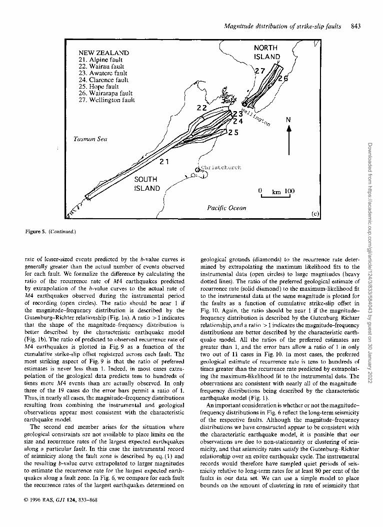
rate of lesser-sized events predicted by the b-value curves is generally greater than the actual number of events observed for each fault. We formalize the difference by calculating the ratio of the recurrence rate of M 4 earthquakes predicted by extrapolation of the b-value curves to the actual rate of M4 earthquakes observed during the instrumental period of recording (open circles). The ratio should be near 1 if the magnitude-frequency distribution is described by the Gutenburg-Richter relationship (Fig. la). A ratio > 1 indicates that the shape of the magnitudefrequency distribution is better described by the characteristic earthquake model (Fig. lb). The ratio of predicted to observed recurrence rate of M4 earthquakes is plotted in Fig. 9 as a function of the cumulative strike-slip offset registered across each fault. The most striking aspect of Fig. 9 is that the ratio of preferred estimates is never less than 1. Indeed, in most cases extrapolation of the geological data predicts tens to hundreds of times more M4 events than are actually observed. In only three of the 19 cases do the error bars permit a ratio of 1. Thus, in nearly all cases, the magnitude-frequency distributions resulting from combining the instrumental and geological observations appear most consistent with the characteristic earthquake model.

The second end member arises for the situation where geological constraints are not available to place limits on the size and recurrence rates of the largest expected earthquakes along a particular fault. In this case the instrumental record of seismicity along the fault zone is described by eq. (1) and the resulting b-value curve extrapolated to larger magnitudes to estimate the recurrence rate for the largest expected earthquakes along a fault zone. In Fig. 6, we compare for each fault the recurrence rates of the largest earthquakes determined on

geological grounds (diamonds) to the recurrence rate determined by extrapolating the maximum likelihood fits to the instrumental data (open circles) to large magnitudes (heavy dotted lines). The ratio of the preferred geological estimate of recurrence rate (solid diamond) to the maximum-likelihood fit to the instrumental data at the same magnitude is plotted for the faults as a function of cumulative strike-slip offset in Fig. 10. Again, the ratio should be near 1 if the magnitude- frequency distribution is described by the Gutenburg-Richter relationship, and a ratio > 1 indicates the magnitude-frequency distributions are better described by the characteristic earthquake model. All the ratios of the preferred estimates are greater than 1, and the error bars allow a ratio of 1 in only two out of 11 cases in Fig. 10. In most cases, the preferred geological estimate of recurrence rate is tens to hundreds of times greater than the recurrence rate predicted by extrapolating the maximum-likelihood fit to the instrumental data. The observations are consistent with nearly all of the magnitude- frequency distributions being described by the Characteristic earthquake model (Fig. 1).

An important consideration is whether or not the magnitude- frequency distributions in Fig. 6 reflect the long-term seismicity of the respective faults. Although the magnitude-frequency distributions we have constructed appear to be consistent with the characteristic earthquake model, it is possible that our observations are due to non-stationarity or clustering of seismicity, and that seismicity rates satisfy the Gutenburg-Richter relationship over an entire earthquake cycle. The instrumental records would therefore have sampled quiet periods of seismicity relative to long-term rates for at least 80 per cent of the faults in our data set. We can use a simple model to place bounds on the amount of clustering in rate of seismicity that

0 1996 RAS, GJI 124, 833-868

Dow




1: SOUTHERN SAN ANDREAS FAULT 100 " " ~ " " ~ " " ~ " " 1 ' ' ' " " ~ ' ~ " '

Mo(mtr)=4 77e+25 dyne-cmlyr

I -: *

: :

J s $ 0 1 - 7 22 2 % .. QD :. 0 . . . . . . . . ....... . . . . . . . .*. 1. k

Mo(mstr)=8 9e+22 3

2 O o l -: Al l shaks

............ . N(M>7)=167 '. . '. - h=O 8 7 s 17

. . O O O l -; : dynecmlyr . . . . ........

ooool': . . . . . . . . . . . . . . . . . : Mo(geol)=4 12 9 72e+24 dyne cmiyr ...... 10.' I ' " ' ; ' " I I " " : " " I " " I " " l ' " ' r

1 : SOUTHERN SAN ANDREAS FAULT

20 1-48

; 5 : - 4 8 g a, 1 5

B 5

L 9

C Q

> - 0 4 8 e z 10 i D : 6

5

0

> - 0 0 4 8

74 a4

10

I

s s $ 0 1

;J 6 g 001

0.

C

0 001

0 0001

SOUTHERN CALIFORNIA . I944 92 N(M>3)=I 3051 h=O86+0 01

10 -:

Ma(geal)=2 72-10 6 1 e t 2 5 dyne-cmlyr 1 0 '

l . " ' I " " I "

y - 480

250

200

k l 5 0

= l o o

50

0

457 M 3 4

Q

5

Mo(mrr)=.2 77e+25 dyne-cmiyr'

6 g 0 o l - r ../ 0 C . . . . . . .

7 4 a4 64year

4 4 54

7 - 4 8 ; 5 ; - 4 8 $

D

i r - * - - 0 4 8 p ! 1 % 1 6

0 001

0 0001

0 048 . . . 0 -: All shocks j N(M>7)=97 /.*. "'.. . b=l 16t023 . . . . . . *

.. I.. '..? . . '. Mo(mrtr)=l Oe+22 . . . . . -; dyne cmiyr : Mo(geol)=2 70-162e+22 dyne c&yr '. '. . '.3 ....,

3: NEWF'ORT-INGLEWOOD FAULT 20

5

0

5

0 7 4 a4

2 3 4 5 6 7 8 9 magnitude

Figure 6 (left-hand column). Discrete number of events per year versus magnitude for the faults listed in Table 2. Faults are numbered according to identification numbers in Tables 1 and 2. Open circles represent the instrumental data; preferred and bounding estimates of the size and recurrence rate of maximum earthquakes derived from fault length and eqs (4) and (5) (Table 2) are shown as solid and open diamonds, respectively; open triangles represent the size and recurrence rate of large earthquakes determined from palaeoearthquake studies (Table 3); heavy dotted lines represent the maximum-likelihood fit to the instrumental data (b-value curves); and light dotted lines bounding the diamonds on each plot have slopes equivalent to the b value of the region that the fault is located within. The number of events greater than the detection threshold magnitude, the b-value fit to the instrumental data, the instrumental moment rate &fo(instr) and number of years of instrumental records represented by the open circles are shown for both the fault (left side) and the enclosing region (top right). The geologically derived moment rate &f,(geol) is also shown at the base of the plots.

Figure 7 (right-hand column). Histograms of the number of earthquakes versus time for the faults listed in Table 2, shown alongside the equivalent magnitudefrequency distribution in Fig. 6. Faults are numbered according to identification numbers in Tables 1 and 2.

0 1996 RAS, GJZ 124, 833-868

Dow



Magnitude distribution of strike-slip faults

4: WHITTIER-ELSINORE FAULT

1 1 1 1 1 1 1 1 1 1 1 1 1 1 1 1 1 1 1 I I I I I

--

_ _

--

-_

_- -

100 i. " ' I " " I " " I " " I " " I " " I ' " . ;

RESNOR (NW BAJA CALIFORNIA)? ' ' N(M>3)=198

I -- @ & h=1.04?0.IS Mn(instr)=1.68e+23 dyne-cm/yr i

0 I - r

2 Open circles: RESNOR -. e,

I0

1 - i

2 9 >r 0.1 2 2 3 8 6 E 0 0 1 2

e,

0.001

:- 16

7 - 1.6 I.

a

SOUTHERN CALIFORNIA 1944-92 N(M>3)=13053 7 - 480

Mo(insu)=4.77e+25 dyne-cmlyr : . . . . . ' . b=O86+0.01 a ' ,,, ._

c e, c)

m

7 -0.048 *. *. - . . 0 . .

dyne-cdyr . . . '0 . . . _ _ . .

50 I I I I I I I I I I I I '

-1 0 m3 D 8 40; 30 I 20

10 - - - I

0 I 1 I 1 I I l-l?n, I

. . . . . . . . * . . Mo(geol)= I .62- I 0.04e+24 dyne-cmlyr * . * * a . -. . . . *. .. *

~ ~ ~ ' " I ~ ~ ~ ~ : ~ ~ " ~ I ~ ' ~ ~ : ~ ~ ~ ~

-

;

2 3 4 5 6 7 8 9

magnitude 5: SAN JACINTO FAULT

2 * 0.01

I I I I I I I " " 1 " " 1 " " 1 " " 1 " " 1 " " ~ " "

Open circles: 1944.92 Closed circle.sS- 1944-92, SOUTHERN CALlFORNlA minus aftershocks 1944.92

480 10 -!-

I

2 22e 0 1 - y E L I

3 2

e,

0.001 - r

0.0001 - Mo(geol)=8.28- 12.42e+24 dyne-c

0.16

0 I

. . . - ' . '. ,

-!976-91

. *. -. . . . . All shocks(RESN0R) * * * ' ' '

2 3 4 5 6 7 8 9

magnitude 11: SAN MIGUEL-VALLECITOS FAULT

10 ~ ~ " " " " " ' I " " : " ! ' " ' : ~ ' ' . ; 1

6 EO.0Ol C 1 N(M>3)=86 /*-....:*,;..' ., 1 b=l l l M . 2 3 . . . .

. Mo(instr)=6.S6e+22 dyke-cm/yi-. .*. ''.:.Q. . . . 0.0001 -r 7

* . .: . . . . .

19. , . , , ;_ Mo(geol)= I .44-3.60e+23 dyne-cmlyr '.' ' . . ' I . ' " I " ' ' I " , ' I . ' ' . I '

7-0.016 u a - 0.0016

2 3 4 5 6 7 8 9 magnitude


35

30

25

20

15

10

5

0 . .

year 54 64

5 : SAN JACINTO FAULT

1 4 0 4

// 40

20

0 44 54 64 74 84

year


845

0 1996 RAS, GJI 124, 833-868

Dow




12: NORTHERN SAN ANDREAS FAULT

230

21 2 r,

E b)

2 3 2 c)

0 2 1 2 x B

0.023

2 3 4 5 6 7 8 9

magnitude 13: CALAVERAS-CONCORD-GREEN VALLEY-BARTLETT SPR

N(M>2)= 1743.5 230 b=0.9?0.01

!- 23

2 2.3 g

f i b) Y

0 2 3 2 51 s

0.023

2 3 4 5 6 7 8 9

magnitude

120

100

80 2 5 60 z

40

20

0

e z

D

L

8 5 z

12: NORTHERN SAN ANDREAS FAULT

L

69 79 Ye=

89

13: CALAVERAS-CONCORD-GREEN VALLE -BARTLE'IT SPRINGS FAULT ZONE

15

10

69 79year 89

14: HAYWARD-ROGERS CREEK-MAACAMA FAULT ZONE

30

25 n

69 79year 89

2 3 4 . 5 6 1 8 9

magnitude

Figure 6. (Continued.) Figure 7. (Continued.)

0 1996 RAS, GJI 124, 833-868

Dow




lo-:

JMA (CENTRAL JAPAN) 7 1926-92 N(M>4 5)=711 b=O 85kO 0 6

Figu

E P

6.6 E 1 e 0

0.6 2 *

2 6

Mo(geol)=6.77-7.74e+24 dyne-cm/yr t 0.0001

2 3 4 5 6 7 8 9

magnitude 16: NEODANI FAULT

I I I I I I I I

JMA (CENTRAL JAPAN) 1926-92

Mo(insrr)=6 82e+25

N(MM 5)=731 b=O 85f0 06

I

2 B g 0.1 2 2 3s .6 E 0.01

2 0001 -:

00001 -; : Mo(geol)4.50-9.0e+23 dyne-cm/yr

L

9" .?_ 6.6 E

1 E 0

-0.6 2 *

3

T 2 3 4 5 6 7 8 9

magnitude 17: ATERA FAULT

I I I I L I I I 100 ~ ' " " " " ' " ' " " " " " ' ' " " " " ' ~

JMA (CENTRAL JAPAN) 1926-92 N(M>4..5)=73 1 b=0.85f0.06 Mo(instr)=6 82e+25 dyne-cmly

J 0 3 mo

0 001

0 om1 Mo(geol)=8 1-14.04e+23 dyne-cmlyr

0 8

t??

k 0 P

6.6 5 c

0.6 2 s 51 a .-

2 3 4 5 6 7 8 9

magnitude

re 6. (Continued.)

8

h 6

z 4

D

5

2

0 26 34 42 50 58 66 74 82 90

Year

16: NEODANI FAULT 8

7

6

5

# 4

3

2

1

0

z'

26 34 42 50 ;Ear 66 74 82 90

17: ATERA FAULT

5

4

h 3

z 2

D

5

1

0 66 14 82 90

42 50 E a r 26 34


0 1996 RAS, GJI 124, 833-868

Dow




18: ATOTSUGAWA FAULT

1 - 7

0 1 - 7

2 2 >1 001 22 2s

a,

5 gJo.00, c

00001

10-5

JMA (CENTRAL JAPAN) 1926-92

b=O 8520 06 Mo(insu)-6 82e+25 dyne cmlyr-

J , - 6 6

10 -r N(M>4 5)=711

1 I

2 a, $ 5 0 1

;g f j gJ 0 0 1 0 6

0 0 0

C

O,e 0 0 001 'F

0 0001 Q -F T

L

-r

-:

-7

-f

18: ATOTSUGAWA FAULT 3 l l l l l l l l l l l ' l l l ' l l l l l l l l l l l l ' l l L

2 . 5 ;

*

I 4 2 :

n 5 1.5: z

1

0.5

0 26 34 42 50 58 66 14 82 90

Yew Mo(geol)=2.70-13 SOe+23 dynexmlyr

2 3 4 5 6 1 8 9

magnitude 19: TANNA FAULT

0 JMA (CENTRAL JAPAN) 1926-92

Mo(instr)=6.82e+25 dyne-cmlyr t N(M>45)=73 1 b=0.8S%C0.06

%m C B O J 0 0 "'g 0.' :

.. 0 Open circles: 1926-92 Closed circles: 1926-92, minus all 1930 shocks

Mo(geol)= I .35-2.7e+21 dyne-cdyr 104

2 3 4 5 6 7 8 9

magnitude 20: YAMASAKI FAULT

10

I

0 1

2 +?i* 0 0 1 2 2 2 2

u

'6 g 0.001 C

0.0001

h. a, 9

6.6 E 1 C a,

0.6 2 Y

51 b"

40

35

30

i 25 0 9 5 20 z

15

10

5

0

19: TANNA FAULT

26 34 42 50 58 66 14 82 90 year

20: YAMASAKI FAULT

4 0 j 1 1 1 1 1 ' 1 1 1 1 1 1 1 1 1 1 1 1 1 1 1 1 ' 1 1 1 1 1 1 1 1 1 1

30

25 :

20 :

15 7

10:

rn3 - -

-

i -

57 I] 14BC

26 34 42 50 ;Ear 66 74 82 90 Mo(geol)=l 08-2 88e+27 dyne-cm/yr

2 3 4 5 6 7 8 9

magnitude


0 1996 RAS, GJI 124, 833-868

Dow




21 : ALPINE FAULT

L

8 2 z

L

8 E, z

35

30

25

20

15

10

5

0 I

84 74 year 64

22: WAIRAU FAULT

84 I4 year 64

2 3 4 5 6 7 8 9

magnitude 23: AWATERE FAULT

23: AWATERE FAULT

L

8 E, z

2 3 4 5 6 7 8 9

magnitude


84 year

64 74


0 1996 RAS, GJI 124, 833-868

Dow




! -2x L B ; - 2 x g

C 0

7 - 0 2 8 2 Y

z

24: CLARENCE FAULT I 1

" ' 1 ' ' " " " ' 1 ' ' " 1 " ' ' 1 " ' " ~ ' ' '

CENTRAL NEW ZEALAND

I I I I I I I I " " " ' " " " ' " " " " " ' " " " ' " ~

CENTRAL NEW ZEALAND . 1964-92 N(M>4)=501

Mp(instr)=2 93e+24 dyne-cdyr : 10 - 7 b=l 09f0 I

L.. I - r / 0 SJ

9; 0 1 1 2 l - 0 0 2 % & 0

1964-92

, b = 1 . 0 9 ~ . I ',, '. N(M>4)=503

. .

'., '. Mo(instr)=2.93e+24 dyne-cmlyr

7- 2x0

7 - 25

, - 2 8

2

C 0

? - 0 2 8 2 .-a

si 6

9 * 0.1

2 g 0.01 c

0.001 4 0.0001 I &o ' . " '.. 0oq '.,.. I. ,, *.. .... , ' .

-:*.. .. .... 0'. All shocks N(M>4)=26 A b=I.OIM.39 . . Mo(instr)=I.O2e+23 *. '.. d yne-cmlyr

. a. -. . . . . . . . .. . . . . . . 1 Mo(geol)=3.24-6 4Xe+24 dyne-cdyr .'. .'*..

t 0.0001

Mo(geol)=l.O9-2 48e+2S dyne-crnlyr

" " I ' " ' I ' ' ~ " ' " ' " ' ~ ' I ~ ~ ' ' I ' " ' 1 2 3 4 5 6 7 8 9

magnitude 26: WAIRARAPA FAULT

24: CLARENCE FAULT

84 74 year 64

25: HOPE FAULT 5

4

3

2

1

0 84

74 year 64

25: HOPE FAULT

n m3

84 74 year

64

26: WAIRARAPA FAULT

l ! l " l l l l " ' l l l l l l l l l ' l ~ l l l l l l ~ 1 .

0 1 1 1 1 1 1 1 1 1 1 1 1 1 1 1 ri I

74 year 64 84


0 1996 RAS, GJI 124, 833-868

Dow




CENTRAL NEW ZEALAND

N(M>4)=501 b=i 1964-92 09+n I

Mo(instr)=Z 97e+24 dyne cm/yr /

100

10

I L cu

2s 0 1 g 2 s18 ‘6 g 0 0 1

C

a ooi

0 0001

10

1 2 8 0

28 5 D

2 8 5 G e, Y

J 0 0

1964-92 N(M>4)=501

Mo(instr)=Z 97e+24 dyne cm/yr i b=i 09+n I

J 0 0

7 - 280

7 - 28

D . - 2 8 5

G e,

5

Y

Mo(geol)=.lS-6.84e+24 dyne-cmlyr t I . . . . I

I I I I

2 3 4 5 6 7 8 9

magnitude

8 23


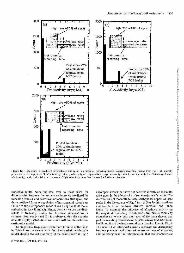
would be necessary for all the faults to have long-term seismicity consistent with the Gutenburg-Richter relationship. We assume that fluctuations in seismicity rates along a fault are reflected by changes in productivity, while the b value remains constant. Further, we note that, on average, the instrumental recording period is about 10 per cent of the return time of the largest earthquakes in each fault, or, in other words, 10 per cent of the earthquake cycle (Fig. l la) , and that the average discrepancy between the actual number of M4 events recorded and the number of M4 events predicted by the geological data is about one order of magnitude (Fig. 1lb). For our analysis, we assume that the average productivity over the entire earthquake cycle for any fault (in this case number of M4 events per year) is equal to 1, but the cycle is divided into periods of ‘high’ and ‘low’ rates of seismicity. We set the ‘low’ rates of seismicity equal to 0.1, consistent with our observations in Fig. l l (b) . The ‘high‘ seismicity rates must therefore be > 1, and would, for example, average 1.9 if they occupied 50 per cent of the cycle. The model is schematically illustrated in Fig. ll(c). With this model, we may use a Monte Carlo approach to answer the question ‘given that seismicity is clustered, the cluster is randomly located in the earthquake cycle, and the instrumental period of recording is limited to 10 per cent of the earthquake cycle (also randomly placed), what is the probability that the rate of seismicity sampled by the instrumental record is less than the long-term average?’ The results are shown by a set of histograms (Fig. 12) for the cases where we have limited ‘high’ seismicity rates to 20 per cent, 30 per cent and 50 per cent of the duration of the cycle, respectively. The histograms show the rates of seismicity predicted in 2000 simulations. Examination of the histograms indicates that ‘high’ seismicity rates must be limited to <20 per cent of the earthquake cycle to yield results similar to our observations (Fig. 12a), that is, 18 out of the 22 faults in the data set showing rates of seismicity less than the predicted long-term average rates (Fig. 6). Similar results are obtained if we assume that the period of ‘high’ rates always occurs at

1 I--

64


m6+1 m5

m3

year 74

ir

84

the same position in the cycle. We also see in Fig. 12(a) that there should be a number of faults that show ‘high’ rates, or, in other words, seismicity rates that are considerably greater than the predicted recurrence rate of M4 in Fig. 6. ‘High rates are clearly observed only along the Yamasaki fault, and uncertainty estimates of predicted M4 recurrence rate might also allow for the possibility of ‘high’ rates on an additional three faults (Figs 6 and 9). Hence, the possibility exists that the seismicity of the faults is described by the Gutenburg- Richter relationship over an entire earthquake cycle, but if so, it appears that extreme clustering is required to argue that this is true. Alternatively, the magnitude-frequency distributions in Fig. 6 may reflect the long-term seismicity of the faults, in which case it is useful to examine the physical ramifications of such an interpretation.

Because geometrical complexities along fault traces appear to control the character of earthquake ruptures (e.g. Seagall & Pollard 1980; Sibson 1985), it is also reasonable to question whether the shape of the magnitude-frequency distribution along faults is also a function of fault-trace complexity. To this end, we further investigate the hypothesis that fault- trace complexity is a decreasing function of cumulative slip (Wesnousky 1988). A trend of decreasing complexity as a function of increasing cumulative slip is evident in Fig. 2, clearly consistent with the early hypothesis. The plot of M4 ratio versus cumulative slip (Fig. 9) therefore allows the possibility that the discrepancy between the predicted and observed numbers of M4 events may be an increasing function of cumulative slip and decreasing fault-trace complexity. The seismicity of faults may therefore initially be characterized by ratios of 1 or less, but with the process of smoothing eventually resulting in the development of a long, throughgoing fault trace, an increase in size of the largest earthquakes, and a decrease in the number of small earthquakes (ratio > l), the latter attributed to a smoothing of the stress field along the fault (e.g. Wesnousky 1990; Ben-Zion & Rice 1993). We might then hypothesize that ongoing cumulative slip eventually

0 1996 RAS, G J I 124, 833-868

Dow



852 M . W. Stirling, S. G. Wesnousky and K. Shimazaki

tl ,_.,‘

’ 1 , , , , , . , , I ;; 6e23*L,-1, , , , , ,I Pref 2e23*L2.1

6e22*L2- 1

0 1 0 2 4

1 o~~ 10 100

Length (km) 1000

Figure 8. Seismic moment versus rupture length for (a) the global data set of major strike-slip faults listed in Romanowicz (1992), and (b) large intraplate earthquakes in Japan (Wesnousky et al. 1983). See the text for further explanation.

causes actual faults to coalesce, so the longest faults are products of the largest amounts of cumulative slip, and have the largest ratios. Additionally, the rate at which fault smoothing and seismicity changes occur might be influenced by the fault slip rate. We investigate these possibilities by plotting the M4 ratio (as used in Fig. 9) against fault length in Fig. 13 and slip rate in Fig. 14. The plots together show that the highest values of ratio tend to be associated with the longest and most rapidly slipping faults. The trend of increasing ratio with both fault length and slip rate (Figs 13 and 14) would imply that the size of the largest earthquakes on a fault

increases and the number of small events decreases as both individual fault strands and faults coalesce to form a long, smooth fault trace, and the rate at which the fault trace becomes longer and smoother depends on the slip rate on the fault. However, the argument that faults lengthen as a direct result of cumulative slip may not be strictly applicable to all strike-slip faults. The San Andreas fault, for instance, has grown in length as a result of northward movement of a plate- boundary triple junction, and not strictly by coalescence of a number of fault strands. Also, it is possible that transform faults that displace thin oceanic crust initiate with relatively

0 1996 RAS, GJI 124, 833-868

Dow




I

0.1 1 10 100 lo00

Strike slip offset (km)

Figure 9. Ratio of the predicted recurrence rate of M4 earthquakes using the regional b value to the observed recurrence rate of M4 earthquakes from the instrumental data versus cumulative strike-slip offset for the faults listed in Table 2. The identification numbers for the faults corresponding to Table 2 are also shown. We show only 19 of the 22 faults listed in Table 2, because cumulative strike-slip displacement measurements are absent for three of the faults. The vertical error bars on each point reflect the maximum and minimum ratios of predicted recurrence rate to observed recurrence rate, while the horizontal error bars represent the uncertainties in the amount of cumulative strike-slip offset.

0.1

1 I I

-- I

24

- 11

t . ' . I .... I I I 1 I I

0.1 1 10 100 1000

Strike slip offset (km)

Figure 10. Ratio of the recurrence rate of maximum-size earthquakes from geological data to the corresponding recurrence rate predicted by extrapolation of the maximum-likelihood fit to the instrumental data versus cumulative strike-slip offset for faults listed in Table 2, and the magnitude-frequency distributions in Fig. 6. The identification numbers for the faults corresponding to Table 2 are also shown. We are unable to represent 11 of the 22 faults listed in Table 2, either because of an absence of cumulative strike-slip displacement measurements, or because it was not possible to fit b-value curves to the very small instrumental data sets for the Japanese faults and several New Zealand faults. The vertical error bars on each point reflect the maximum and minimum ratios of the bounding geological estimates (open diamonds in Fig. 6) to the 95 per cent confidence limits on the extrapolated b-value curves (upper and lower heavy dotted lines), and the horizontal error bars reflect the uncertainties in the amount of cumulative strike-slip offset.

simple traces, so minimal step reduction would occur with ongoing cumulative slip. In general, the different tectonic environments represented in our data set will influence the rates of fault smoothing and lengthening, and so contribute to the scatter evident in Figs 2, 9, 10, 13 and 14.

Although our estimates of recurrence rate are based on

geological observations, they are also model-dependent (eqs 4 and 5). The use of total fault length in deriving maximum earthquake size may be inconsistent with observations in areas like California, where the largest historical earthquakes may arise from rupture of segments of the faults less than the total fault lengths. However, assumption of a smaller rupture length

0 1996 RAS, GJI 124, 833-868

Dow




0 0.05 0.1 0.15 0.2 0.25 0.3 0.35

Ratio instrumental recording timeheturn time

-2 -1 0 1 2 3 4 Log Preferred Frequency Ratio

(predicted M4dyr / observed M4 n/yr)

Instrumental recording period (1 0% of earthqu\ake cycle)

1

0.1

0 TIME 1

Figure 11. (a) Histogram of the ratio of instrumental recording time to the return time of the largest earthquakes for the faults listed in Table 2. (b) Histogram of the log of the preferred frequency ratio (predicted/observed recurrence rate of M4 earthquakes, or middle light dotted line in Fig. 6) for the faults listed in Table 2. The preferred ratios and uncertainty estimates (min and max ratios) are generally in the range 10 to 100 (log ratio = 1 to 2). (c) A simple model of an earthquake cycle, whereby seismicity is consistent with the Gutenburg- Richter relationship over the entire cycle, but the cycle is characterized by periods of 'low' and 'high' seismicity rates (clustering). The model shows clustering into 20 per cent of the earthquake cycle, and an instrumental recording period that is 10 per cent of the cycle.

on a fault will only add more support to our interpretation of Fig. 6, that most of the faults show a characteristic earthquake distribution. Assumption of a lesser maximum fault rupture length predicts a smaller maximum earthquake M:, but interpretation of the smaller value with eqs (4) and (5) also predicts that it should occur more frequently. The net result is then to generally increase the discrepancy between the geological estimates and the extrapolation of the instrumental record. One may also consider the possibility of ruptures extending beyond our defined fault lengths, and factor larger values of Mz into eqs (4) and (5). The tendency will be to reduce the predicted recurrence rates of M z , and therefore reduce the discrepancy between geological and extrapolated instrumental recurrence rates. However, the recurrence rates will only be reduced significantly in terms of our interpretation of Fig. 6 if on average ME is increased about 30-fold. It seems physically unrealistic to consider increasing Mz by this amount on those faults we have considered.

There may be some bias in our calculations because we assume that the majority of seismic moment is released during the repeated occurrence of earthquakes of the same size. The concern can be addressed by further assuming that seismicity satisfies the Gutenburg-Richter relationship up to the maximum expected event defined by assuming rupture of the entire fault length. Seismic moment is therefore also released by events close in size but <Mmax, and the recurrence rate of the events across the entire magnitude range can be calculated by using estimates of Mmax, b value and slip rate for each fault. Following the approach of Wesnousky et al. (19831, and using the estimate of Mmax, slip rate, and b value for each fault, we calculate and show in Fig. 15 the expected number of M4 earthquakes for each of the faults in the data set versus the actual observed number of events. On average, the predicted recurrence rates are about 10 times greater than the observed values. The discrepancy is consistent with the characteristic earthquake model. Hence, the principal observations and interpretations made from Figs 6, 9 and 10 are apparently not significantly altered if a distribution of large earthquakes is allowed.

Our estimates of earthquake recurrence rates along the faults estimated from eqs (4) and (5) may also be compared to estimates of earthquake size and recurrence that come directly from trenching studies, where the estimation of large surface rupturing events is determined directly from structural and stratigraphic analysis of offset sediments in the trench. Similarly, historical data define the sizes of large earthquakes for a number of the faults listed in Table2. The results of trenching studies and historical observations are summarized in Table 3 and Appendix A, and plotted as open triangles in Fig. 6. For the majority of the faults, the estimates of earthquake size and recurrence rate resulting from palaeoearthquake and historical data (triangles in Fig. 6) fall within or close to the uncertainties in our estimates based on fault length and eqs (4) and ( 5 ) (diamonds). It is only along the Whittier- Elsinore, Calaveras-Concord-Green Valley-Bartlett Springs and San Jacinto faults that predicted recurrence rates and event sizes resulting from trenching and historical records do not fall within the bounds resulting from application of eqs (4) and (5). The discrepancies probably reside in the trenching studies and historical observations, reflecting the occurrence of events that rupture less than the entire length of the

0 1996 RAS, GJI 124, 833-868

Dow




l ~ l ' l ~ l ~ l ~ l ' l ' l ~ l ~

High rate =30% of cycle : (b)

- -

2000

1500

G I .c,

3 1000

500

0

2000

1500 Y

3 1000

500

0

- Instrumental recording time

Pro61 for 35%- of simulations (equivalent to . J/ I . 1 . 1 . 1 . 1 . 7/22 faults) I .

0 1 2 3 4 5 6 7 8 9 10

High rate =20% of cycle

-

Instrumental recording time

Prod>l for 27% of simulations (equivalent to 6/22 faults)

0 1 2 3 4 5 6 7 8 9 1 Productivity (dyr; M4) 0

l ' l ' l * l ' l ' l ' l ' l ' l '

- (4 High rate =50% of cycle -

- A / -

- Instrumental - recording time -

P r o b l for about 50% of simulations

/ (equivalent to 11/22

-

0 1 2 3 4 5 6 7 8 9 1 Productivity (n/yr; M4) 0

2000

1500 +I

E: s u 1000

500

0

Productivity (n/yr; M4)

Figure 12. Histograms of predicted productivity during an instrumental recording period (average recording period from Fig. 1 la), whereby productivity < 1 represents 'low' seismicity rates, productivity = 1 represents average seismicity rates (consistent with the Gutenburg-Richter relationship), and productivity > 1 represents 'high' seismicity rates. See the text for further explanation.

respective faults. None the less, even in these cases, the encompass events that have not occurred directly on the faults, discrepancies between the recurrence intervals predicted by most notably the aftershocks of some major earthquakes. The trenching studies and historical observations (triangles) and distributions of moderate to large earthquakes appear as large those predicted from extrapolation of instrumental records are peaks in the histograms of Fig. 7 for the San Jacinto, northern similar to the discrepancies found when using the fault model and southern San Andreas, Awatere, Yamasaki and Tanna embodied in eqs (4) and ( 5 ) . Hence, whether we use the direct faults. To examine the influence of aftershock activity on results of trenching studies and historical observations or the magnitude-frequency distributions, we remove seismicity estimates from eqs (4) and ( 5 ) , it is observed that the majority occurring up to one year after each of the main shocks, and of faults display distributions consistent with the characteristic plot the resulting recurrence rates (solid circles) and maximum- earthquake model. likelihood fits to the instrumental data (hatched lines) in Fig. 6.

The magnitude-frequency distributions for most of the faults The removal of aftershocks clearly increases the discrepancy in Table 2 are consistent with the characteristic earthquake between predicted and observed recurrence rates of all events, model, despite the fact that many of the boxes shown in Fig. 5 and so strengthens the interpretation that the characteristic

0 1996 RAS, G J I 124, 833-868

Dow



856 M. W, Stirling, S. G . Wesnousky and K . Shimazaki

0.1

0.01

I I I I 1 1 1 1 1 , I I I I I I I

- L v s o u t h e r n CalifornidBaja Calif A northern California

17

18

- New Zealand

Japan

- 19

-- - 7 - - 1

I 1

10 100 Fault length (km)

lo00

Figure 13. Ratio of the predicted recurrence rate of M4 earthquakes using the regional b value to the observed recurrence rate of M4 earthquakes from the instrumental data versus fault length for the faults listed in Table 2. The identification numbers for the faults corresponding to Table 2 are also shown. The vertical error bars reflect the maximum and mimimum ratios (as in Fig. 9). The Yamasaki fault is the only fault that shows a preferred value of ratio of less than 1; it was not represented in the earlier plots due to the absence of an estimate of cumulative strike-slip offset (Table 1).

0.1

0.01

northern California

0.1 1 10 Slip rate ( d y r )

100

Figure 14. Ratio of the predicted recurrence rate of M4 earthquakes using the regional b value to the observed recurrence rate of M4 earthquakes from the instrumental data versus slip rate for the faults listed in Table 2. The identification numbers of the faults corresponding to Table 2 are also shown. The vertical error bars reflect the maximum and mimimum ratio (as in Fig. 9), and horizontal error bars represent uncertainties in the fault slip rates.

CONCLUSIONS earthquake model best describes the seismicity of the faults. We d o not attempt to alter our box widths to selectively exclude ‘background‘ seismicity that we observe in the crustal Magnitude-frequency distributions from a data set of 22 blocks adjacent to the faults, but, in light of the above, the strike-slip faults from around the world are generally effect of doing this would be to increase the discrepancy consistent with the characteristic earthquake model, whereby between predicted and observed recurrence rates. geological estimates of the recurrence rate of the largest

0 1996 RAS, GJI 124, 833-868

Dow




Table 3. Magnitude and average return time estimates for the largest earthquakes arising from palaeoseismic studies and historical observations for the faults listed in Table 2. Data sources are as follows: (1) Sieh (1978); Sieh & Jahns (1984); (4) Pinault & Rockwell (1984); Rockwell et al. (1985, 1986); Brake & Rockwell (1987); (5) Sharp (1981); Clark (1972); Clark, Grantz & Rubin (1972); Burdick & Mellman (1976); Bent et al. (1989); Hudnut & Sieh (1989); Magistrale, Jones & Kanamori (1989); Lindvall, Rockwell & Hudnut (1989); Rockwell et al. (1990); (11) Hirabayashi et al. (1993); (12) Lawson (1908); Thatcher (1975); Sieh (1978); (13) Wesnousky (1986); (14) Toppozada, Real & Parke (1981); Budding et al. (1991); Williams (1991) (15,16) Okada & Ikeda (1991); (17) Awata et al. (1986); Okada & Ikeda (1991); (18-20) Okada & Ikeda (1991); (21) Hull & Berryman (1986); (22) Lensen (1976); Johnston (1990); (23) 66m lateral offset of 9410,1570yr terraces (Knuepfer 1992), and 6 m single event displacement of 1848, magnitude 7.1 Marlborough earthquake (Lensen 1978) indicate 1 1 earthquakes in 9410 yr = average return time of 855 yr; (25) Cowan & McGlone (1991); (26) Wellman (1972); Darby & Beanland (1992); (27) Berryman (1990): Van Dissen et al. (1992).

ID&FAULT LOCATION MAGNITUDE RJXURN TIME

Southern California 1. Southern San Andreas

4. Whittier-Elsinore

5 . San Jacinto

11. San Miguel-Vallecitos

Parkfield-Cajon Pass

Corona-Lake Elsinore Coyote Mtn Coyote Creek fault Superstition Hills fault Las Cuevitas-Jamu

7.8

6.2 6.5-7 6.5 6.6 6.8

350 yrs

175yrs 800 F 7Oyrs

225yrs 2830 yrs

Northern California 12. Northern San Andreas Mendocino-San Juan Bautista

13. Calaveras-Concord-Green northern Calavwas fault Valley-Bartlett Sp 14. Hayward-Rogers Ck Hayward fault - M a a c m Rogers Ck fault

7.7

6.1

6.8 7

300 yrs

l50yrs

325yrs 464 F

~

Japan 15. Median Tectonic Line Shikoku Island 8 1000 yrs

16. Neodani Central Japan 8 10000 yrs

17. Atera Cenrral Japan 7.8 1700 yrs

1 8. Atotsugawa Central Japan 7 1700 yrs

19. Tanna North Izu 7.3 850 yrs

20. Yamasah West central Japan 7-7.4 2550 yrs

New Zcaland 21. Alpine south Westland

23. Awatere Awatere valley

25. Hope Hope River

26. Wairarapa southern Wairarapa

27. Wellington Wellington-Hutt Valley

7.4-8

7.1

7.3

8

7.1-7.8

426 yrs

855 yrs

148 yrs

1400 yrs

600 yrs

earthquakes are orders of magnitude more frequent than rates predicted from interpretation of earthquake statistics. It is possible that the magnitude-frequency distributions may simply be an artefact of a short instrumental recording period, and seismicity over an entire earthquake cycle is instead described by the Gutenburg-Richter relationship. However, such an interpretation requires that seismicity along faults be limited or clustered in periods of time less than or equal to about 20 per cent of the return period of the largest expected earthquakes on a fault. We suggest that the observed magnitude-frequency distributions do reflect the long-term character of seismicity along faults. The suggestion allows the possibility that the ratio of small to large earthquakes along a fault decreases with increasing cumulative slip. We observe that fault-trace complexity is a decreasing function of cumulative slip, a smoothing process that would allow for longer rupture lengths and a more

homogenous stress field along the fault, therefore increasing the size of the largest earthquakes and reducing the number of small earthquakes. Regardless of a physical basis for the characteristic earthquake model, the model is more appro- priate than the Gutenburg-Richter relationship in describing the seismicity of strike-slip faults for seismic hazard analysis.

ACKNOWLEDGMENTS

We wish to thank Warwick Smith, Terry Webb, Kelvin Berryman, Sarah Beanland, David Oppenheimer, Takashi Kumamoto, and Raul Castro for providing access to earthquake catalogues and other digital data. Reviews of the manuscript by John Anderson, Jim Brune and an anonymous reviewer were beneficial, and useful comments were provided by Rachel Abercrombie, Yehuda Ben-Zion,

0 1996 RAS, GJI 124, 833-868

Dow



858 M . W Stirling, S. G. Wesnousky and K . Shimazaki

loo I I

Southern CaliforniaEhja Calif I 21 4 Northern California

New Zealand

l i

3

11 I 1 I I/ , , , , j , , , I I I 0.01 I

0.01 0.1 1 10 Observed dyr(M4)

Figure 15. Recurrence rates of M4 earthquakes predicted by using estimates of slip rate (Table 1) and M""" (Table 2), and by assuming that seismicity is distributed in accord with the Gutenburg-Richter relationship for all magnitudes up to Pax (Wesnousky et al. 1983), versus the observed recurrence rate of M4 earthquakes from the instrumental data. The identification numbers for the faults corresponding to Table 2 are shown. We also show that the predicted and observed recurrence rates for the entire 1000 km length of the San Andreas fault, and for the 200 km combined length of the Newport-Inglewood-Rose Canyon faults (open symbols) are similar to those of the much shorter northern San Andreas, southern San Andreas, and Newport-Inglewood faults (I , 12 and 3).

John Caskey, Craig dePolo, Mark Petersen, and Euan Smith. Thanks go to Yu Guang and Qingbin Chen for help with translating Chinese publications. The research was partially supported by the Southern California Earthquake Center (publication no. 206) and USGS (contract 1434-94- G-2460). Center for Neotectonic Studies Contribution Number 15.

REFERENCES

Aki, K., 1965. Maximum likelihood estimates of b in the formula log N = a - bM and its confidence limits, Bull. Earthq. Res. Inst.,

Aki, K. & Richards, P.G., 1980. Quantitatiue Seismology: Theory and Methods, W.H. Freeman, San Francisco, California.

Anderson, J.G., Rockwell, T. & Agnew, D., 1989. A study of seismic hazard of San Diego, Earthq. Spectra, 5, 299-333.

Awata, Y., Mizuno, K., Tsukuda, E. & Yamazaki, H., 1986. The recurrence interval of faulting on the Atera fault and the age of its last activity, Program and abstracts, Jpn. Assoc. Quat. Res., 16,

Barka, A.A. & Gulen, L., 1988. New constraints on age and total offset of the north Anatolian fault zone: Implications for tectonics of the eastern Mediterranean region, in Spec. Publ. Middle East Tec. Uniu., Meloh Tokay Geology Symposium, Ankara, Turkey.

43, 237-239.

132-133.

Barka, A.A. & Kadinsky-Cade, K., 1988. Strike-slip fault geometry in Turkey and its influence on earthquake activity, Tectonics, 7,

Barrows, A.G., 1974. A review of the geology and earthquake history of the Newport-Inglewood structural zone, southern California, Spec. Rep., California Division of Mines and Geology, 114.

Bent, A.L., Helmberger, D.V., Stead, R.J. & Ho-Liu, P., 1989. Waveform modeling of the November 1987 Superstition Hills earthquakes, Bull. seism. Soc. Am., 79, 500-513.

Ben-Zion, Y. & Rice, J.R., 1993. Earthquake failure sequences along a cellular fault zone in a 3D elastic solid containing asperity and nonasperity regions, J. geophys. Res., 98, 14 109-14 131.

Berryman, K.R., 1990. Late Quaternary movement on the Wellington Fault in the Upper Hutt area, New Zealand, N.Z. J . Geol. Geophys., 33, 257-270.

Berryman, K.R. & Beanland, S., 1988. The rate of tectonic movement in New Zealand from geological evidence, Trans. Inst. Prof. Eng.

Brake, J.F. & Rockwell, T.K., 1987. Magnitude of slip from historical and prehistorical earthquakes on the Elsinore fault, Glen Ivy marsh, southern California, Geol. SOC. Am. Abstr. with Programs, 19.

Brown, R.D., 1970. Map showing recently active breaks along the San Andreas and related faults between the northern Gabilan Range and Cholame Valley, California, USGS Misc. geol. Invest. Map, 1-575.

Brown, R.D. & Wolfe, E.W., 1972. Map showing recently active breaks along the San Andreas fault between Point Delgada and Bolinas Bay, California, USGS M i x . geol. Invest. Map, 1-692.

663-684.

N.Z., 15, 25-35.

0 1996 RAS, G J I 124, 833-868

Dow




Browne, G.H., 1992. The northeastern portion of the Clarence fault: tectonic implications for the late Neogene evolution of Marlborough, New Zealand, N.Z. J. Geol. Geophys., 35, 437-446.

Brune, J.N., 1968. Seismic moment, seismicity and rate of slip along major fault zones, J. geophys. Rex, 73, 777-784.

Budding, K.E., Schwartz, D.P. & Oppenheimer, D.H., 1991. Slip rate, earthquake recurrence, and seismogenic potential of the Rogers Creek fault zone, northern California: initial results, Geophys. Res. Lett., 18, 441-450.

Burdick, L. & Mellman, G.R., 1976. Inversion of body waves from the Borrego Mountain earthquake to source mechanism, Bull. seism. Soc. Am., 66, 1485-1499.

California Division of Mines and Geology, 1992. Preliminary fault activity map of California, DMG openfile report, 92-03.

Clark, M.M., 1972. Surface rupture along the Coyote Creek fault, the Borrego Mountain earthquake of April 9, 1968, USGS Prof. Paper,

Clark, M.M., 1973. Map showing recently active breaks along the Garlock and associated faults, California, USGS Misc. Geol. Invest. Map, 74.

Clark, M.M., 1984. Map showing recently active breaks along the San Andreas fault and associated faults between Salton Sea and Whitewater River-Mission Creek, California, USGS Misc. Field. Invest. Map, 1-1483.

Clark, M.M., Grantz, A. & Rubin, M., 1972. Holocene activity of the Coyote Creek fault as recorded in sediments of Lake Cahuilla. The Borrego Mountain Earthquake of April 9, 1968, USGS Prof. Paper,

Cowan, H.A., 1990. Late Quaternary displacements on the Hope fault at Glynn Wye, North Canterbury, N.Z. J. Geol. Geophys., 33, 285-294.

Cowan, H.A., 1991. The North Canterbury earthquake of September 1,

Cowan, H.A. & McGlone, M.S., 1991. Late Holocene displacements and characteristic earthquakes on the Hope River segment of the Hope Fault, New Zealand, J. R . Soc. N.Z., 21, 373-384.

Crowell, J.C., 1962. Displacement along the San Andreas fault, California, Geol. SOC. Am. Spec. Paper, 7, 61.

Darby, D.J. & Beanland, S., 1992. Possible source models for the 1855 Wairarapa earthquake, New Zealand, J . geophys. Res., 97(B9), 12 375-12 390.

Dokka, R.K., 1983. Displacements on late Cenozoic strike-slip faults of the central Mojave Desert, California, Geology, 11, 305-308.

Freund, R., 1971. The Hope fault, a strike-slip fault in New Zealand, N.Z. geol. Surv. Bull., 86, 1-49.

Galehouse, J.S., 1991. Creep rates on the Bay Area faults during the past decade, Seism. Res. Lett., 62, 12 (abstract).

Gastil, R.G., Phillips, R.P. & Allison, E.C., 1975. Reconnaissance geologic map of the State of Baja California, Mexico, Geol. Soc. of Am. Mem., 140.

Given, D., Hutton, L., & Jones L.M., 1987. The Southern California Network Bulletin, July-December, 1986 USGS Open File Rpt.

Grantz, A. & Dickenson, W.R. 1968. Indicated cumulative offsets along the San Andreas fault in California Coast Ranges, in Proc. Conf geol. problems San Andreas fault system, eds. Dickenson, W.R. & Grantz, A., Stanford University Publication XI, 117-120.

Gutenburg, B. & Richter, C.F., 1944. Frequency of earthquakes in California, Bull. seism. SOC. Am., 34, 185-188.

Hanks, T.C. & Kanamori, H., 1979. A moment magnitude scale, J. geophys. Res., 84, 2348-2350.

Harvey, T.W., 1985. Geology of the San Miguel fault zone, northern Baja California, Mexico, PhD thesis, San Diego State University.

Herd, D.G., 1979. Neotectonic framework of central California and its implications to microzonation of the San Francisco Bay region, USGS Circular, 807, 3-12.

Herd, D.G., 1988. Map of active traces of Hayward-Macaama and

787, 55-86.

787, 112-130.

1888, J . R . SOC. N.Z., 21, 1-12.

87-488.

Calaveras-Rogers Creek-Green Valley fault zones at 1 : 250000 scale (unpublisbed map).

Herd, D.G. & Helley, E.J., 1977. Faults with Late Quaternary displacement, Northern San Francisco Bay region, California, 1 : 125000. USGS Misc. Field Studies Map, MF818.

Hill, R.I., 1981. Geology of Garner Valley and Vicinity, in Geology of the Sun Jacinto Mountains, Field Trip Guide 9, pp. 90-99, eds Brown, A.R. & Ruff, R.W., South Coast Geol. SOC., Irvine, California.

Hirabayashi, K.C., Rockwell, T.K. & Wesnousky, S.G., 1993. Clustering of seismic activity on the San Miguel fault, Baja California, Mexico, EOS, Trans. Am. geophys. Un., 74 (43), 515.

Hirabayashi, K.C., Rockwell, T.K., Wesnousky, S.G., Stirling, M.W. & Suarez-Vidal, F., 1996. A neotectonic study of the San Miguel- Vallecitos fault, Baja California, Mexico, Bull. seism. SOC. Am., in press.

Hope, R.A., 1969. Map showing recently active breaks along the San Andreas and related faults between Cajon Pass and Salton Sea, USGS Open File Rpt, 69-130.

Hudnut, K.W. & Sieh, K.E., 1989. Behavior of the Superstition Hills fault during the past 330 years, Bull. seism. SOC. Am., 79, 304-329.

Hull, A.G. & Berryman, K.R., 1986. Holocene tectonism in the region of the Alpine fault at Lake McKerrow, Fiordland, New Zealand,

Hull, A.G. & Nicholson, C., 1992. Seismotectonics of the Northern Elsinore fault zone, Southern California, Bull. seism. SOC. Am.,

Institute of Geological and Nuclear Sciences Ltd, 1994. Unpublished active fault database.

Institute of Geology, 1990. The Haiyuan Active Fault Zone, Special Issue, Beijing, China (in Chinese).

Institute of Geology, 1991. The Altun Fault Zone, Special Issue, Beijing, China (in Chinese).

Ishimoto, M. & Iida, K., 1939. Observations sur les seisms enregistre par le microseismograph construite dernierment (I), Bull. Earthqu. Res. Inst. Univ. Tokyo, 17, 443-478.

Johnston, M.R., 1990. Geology of the St Arnaud District, Southeast Nelson (Sheet N29), N.Z. geol. Surv. Bull., 99.

Kintzer, F.C., Brooks, J.C. & Cummings, J.C., 1977. An offset Miocene shoreline: implications for Calaveras fault movement, Geol. Soc. Am. Abstr. programs, 9, 65.

Knuepfer, P.L.K., 1992. Temporal variations in latest Quaternary slip across the Australian-Pacific plate boundary, northeastern South Island, New Zealand, Tectonics, 11, 449-464.

Lawson, A.C., 1908. The San Andreas rift as a geomorphic feature, in Rpt. State Earthq. Investigation Committee Vol 1, The Calfornia Earthquake of April 18 1906, 25-115.

Lee, W.H.K., Bennett, R.E. & Meagher, K.L., 1972. A method of estimating magnitude of local earthquakes from signal duration, USGS Open File Rpt., 28.

Lensen, G.J., 1960. A 12 mile lateral drag along the Awatere fault, Abstr. 9th Sci. Cong., R . SOC. N.Z., 47.

Lensen, G.J., 1976. Sheets N28D, 028C and N29B-Hillersden; sheets 028BD, P28A and P28C-Renwick, Late Quaternary tectonic map of New Zealand 1 :50,000, Dept sci. indust. Res., Wellington, New Zealand.

Lensen, G.J., 1978. Historic tectonic earth deformation, in The Geology of New Zealand, pp.33-39, eds Suggate, R.P., Stevens, G.R. & Te Punga, M.T., Government Printer, Wellington, New Zealand.

Lienkaemper, J.J., Borchardt, G. & Lisowski, M., 1991. Historic creep rate and potential for seismic slip along the Hayward fault, California, J. geophys. Res., 96, 18 261-18 283.

Lindvall, S.C., Rockwell, T.K. & Hudnut, K.W., 1989. Slip distribution of prehistorical earthquakes on the Superstition Hills fault, San Jacinto fault zone, southern California, based 011 offset geomorphic features, Abstr. with Programs, Geol. Soc. Am., 21, 107.

Magistrale, H., Jones, L. & Kanamori, H., 1989. The Superstition Hills, California earthquakes of 24 November 1987, Bull. seism. SOC. Am., 79, 239-251.

R . SOC. N.Z. Bull., 24, 317-331.

82, 800-818.

0 1996 RAS, GJI 124, 833-868

Dow



860 M. W. Stirling, S. G. Wesnousky and K . Shirnazaki

Matsu’ura, M., Jackson, D.D. & Cheng, A,, 1986. Dislocation model for aseismic crustal deformation at Hollister, California, J. geophys. Res., 91, 12 661-12 674.

Matti, J.C., Morton, D.M. &Cox, B.F., 1985. Distribution and geologic relations of fault systems in the vicinity of the Central Transverse ranges, southern California, USGS Open File Rpt., 85-365.

Mochizuki, E., Kobayashi, E. & Kishio, M., 1978. Hypocenter determination ability of JMA seismological observation system during 1965-1974, Q. J . Seism., 42, 23-30 (in Japanese).

Morton, D.M., Miller, F.K. & Smith, C.C., 1980. Photo-reconnaissance maps showing young-looking fault features in the southern Mojave Desert, California, USGS Misc. Field Studies Map, MF-1051.

Officers of the New Zealand Geological Survey, 1983. Late Quaternary tectonic map of New Zealand 1 : 2,000,000, 2nd edn, N.Z. geol. Surv. Misc. Series Map 12, Dept Sci. Indus. Res., Wellington, New Zealand.

Okada, A., 1980. Quaternary faulting along the Median Tectonic Line of Southwest Japan, in The Median Tectonic Line of Southwest Japan, Mem. geol. SOC. Jpn, 18, pp, 79-108, ed. Ichikawa, K.

Okada, A. & Ikeda, Y., 1991. Active faults and neotectonics in Japan, Quat. Res., 30, 161-174.

Petersen, M.D. & Wesnousky, S.G., 1994. Fault slip rates and earthquake histories for active faults in southern California, Bull. seism. Soc. Am., 84, 1608-1649.

Pinault, C.T. & Rockwell, T.K., 1984. Rates and sense of Holocene faulting on the southern Elsinore fault: Further constraints on the distribution of dextral shear between the Pacific and North American plates, Geol. SOC. Am. Abstr. with Programs, 16, 624.

Prentice, C.S., Niemi, T.M. & Hall, T.M., 1993. Quaternary tectonics of the northern San Andreas fault, San Francisco Peninsula, Point Reyes, and Point Arena, California, USGS Fieldtrip Guide, S.F. Peninsula Transect.

Radbrush-Hall, D.H., 1974. Map showing recently active breaks along the Hayward Fault zone and the southern part of the Calaveras fault zone, California, USGS Misc. Invest. Series Map, 1-813.

Research Group for Active faults of Japan, 1992. Map of active faults in Japan with an explanatory text, University of Tokyo Press, Tokyo.

Rockwell, T.K., Loughman, C. & Merifield, P., 1990. Late Quaternary rate of slip along the San Jacinto fault zone near Anza, southern California, J. geophys. Res., 95, 8593-8605.

Rockwell, T.K., Lamar, D.L., McElwain, R.S. & Millman, D.E., 1985. Late Holocene recurrent faulting on the Glen Ivy north strand of the Elsinore fault, southern California, Geol. SOC. Am. Abstr. with Programs, 17, 404.

Rockwell, T.K., McElwain, R.S., Millman, D.E. & Lamar, D.L., 1986. Recurrent late Holocene faulting on the Glen Ivy north strand of the Elsinore fault at Glen Ivy marsh, Neotectonics and Faulting in southern California, Cordilleran section, Geol. SOC. Am., Guidebook, 167-1275.

Romanowicz, B., 1992. Strike-slip earthquakes in quasi-vertical transcurrent faults: Inference from general scaling relations, Geophys. Res. Lett., 2, 56-59.

Ross, D.C., 1969. Map showing recently active breaks along the San Andreas fault between Tejon Pass and Cajon Pass, southern California, USGS Misc. j e l d Inoest. Map, 1-553.

Savage, J.C., Prescott, W.H., Lisowski, M. & King, N., 1979. Geodetic measurements of deformation near Hollister, California, 1971-1978, J. geophys. Res., 84, 7599-7615.

Schwartz, D.P. & Coppersmith, K.J., 1984. Fault behavior and characteristic earthquakes: Examples from the Wasatch and San Andreas fault zones, J . geophys. Res., 89, 5681-5698.

Seagall, P. & Pollard, D.D., 1980. Mechanics of discontinuous faults, J . geophys. Rex, 85(B8), 4337-4350.

Sharp, R.V., 1975. En echelon fault patterns of the San Jacinto fault zone, Southern California, Bull. Cal f . Diu. Mines Geol, 196, 187-194.

Sharp, R.V., 1981. Variable rates of late Quaternary strike-slip on the San Jacinto fault zone, southern California, J. geophys. Res., 86, 1154-1762.

Sibson, R.H., 1985. Stopping of earthquake ruptures at dilatational fault jogs, Nature, 316, 248-251.

Sieh, K.E., 1978. Slip along the San Andreas fault associated with the great 1857 earthquake, Bull. seism. SOC. Am., 68, 1421-1448.

Sieh, K.E. & Jahns, R.H., 1984. Holocene activity of the San Andreas fault at Wallace Creek, California, Geol. SOC. Am. Bull., 95, 883-896.

Smith, G.I., 1962. Large lateral displacement on the Garlock fault, California, as measured from offset dike swarm, Bull. Am. Assoc. petrol. Geol., 46, 85-104.

Smith, W.D., 1976. A computer file of New Zealand earthquakes, N.Z. J . Geol. Geophys., 19, 393-394.

Thatcher, W., 1975. Strain accumulation and release mechanism of the 1906 San Francisco earthquake, J . geophys. Res., 80, 4862-4872.

Toppozada, T.R., Real, C.R. & Parke, D.L., 1981. Preparation of isoseismal maps and summaries of reported effects for pre-1900 California earthquakes, California Division of Mines and Geol. Open File Rpt, 81-11.

Utsu, T., 1965. A method for determining the value of b in a formula log n = a - bM showing the magnitude-frequency relation for earthquakes, Geophys. Bull. Hokkaido University, 13,99-103 (in Japanese).

Utsu, T., 1982. Relationships between earthquake magnitude scales, Bull. Earthq. Res. Inst., Univ. Tokyo, 57, 465-497.

Van Dissen, R.J. & Yeats, R.S., 1991. Hope fault, Jordan thrust, and uplift of the Seaward Kaikoura Range, New Zealand, Geology,

Van Dissen, R.J., Berryman, K.R., Pettinga, J.R. & Hill, N.L., 1992. Paleoseismicity of the Wellington-Hutt Valley segment of the Wellington fault, North Island, New Zealand, N.Z. J . Geol. Geophys.,

Vedder, J.B. & Wallace, R.E., 1970. Map showing recently active breaks along the San Andreas and related faults between Cholame Valley and Tejon Pass, California, USGS Misc. geol. Invest. Map,

Vidal, A. & Munguia, L., 1993. Ten years of functioning of the seismic network of northwestern Mexico, Ciencia y Desarrollo, 18, 77-85 (in Spanish).

Wellman, H.W., 1953. Jurassic-Recent data for the study of Recent and late Pleistocene faults in the South Island of New Zealand, N.Z. J . Sci. Tech., B34, 270-288.

Wellman, H.W., 1972. Rate of horizontal fault displacement in New Zealand. Nature, 237, 275-277.

Wesnousky, S.G., 1986. Earthquakes, Quaternary faults and seismic hazard in California, J. geophys. Res., 91, 12 587-12 631.

Wesnousky, S.G., 1988. Seismological and structural evolution of strike-slip faults, Nature, 335, 340-343.

Wesnousky, S.G., 1990. Seismicity as a function of cumulative geologic offset: Some observations from southern California, Bull. seism. SOC. Am., 80, 1374-1381.

Wesnousky, S.G., 1994. The Gutenburg-Richter or Characteristic Earthquake Distribution, which is it?, Bull. seism. SOC. Am., 84,

Wesnousky, S.G., Scholz, C.H., Shimazaki, K. & Matsuda, T., 1983. Earthquake frequency distribution and the mechanics of faulting, J. geophys. Res., 88(Bll), 9331-9340.

Williams, P.L., 1991. Evidence of late Holocene ruptures, southern Hayward fault, California, Seism. Res. Lett., 62, 14 (abstract).

Working Group on California Earthquake Probabilities, 1990. Probabilities of large earthquakes occurring in California on the San Andreas fault, USGS Open File Rpt, 88-398, 62.

Yang, J.S., 1991. The Kakapo fault-a major active dextral fault in the central North Canterbury-Buller regions of New Zealand, N.Z. J . Geol. Geophys., 34, 137-143.

Yokoyama, H., 1984. Epicenter determination ability of the recent JMA network: 1979-1983, Q. J. Seism., 49, 53-65 (in Japanese).

Youngs, R.R. & Coppersmith, K.J., 1985. Implications of fault slip rates and earthquake recurrence models to probabilistic seismic hazard estimates, Bull. seism. Soc. Am., 75 , 939-964.

19, 393-396.

35, 165-176.

1-574.

1940-1959.

0 1996 RAS, GJI 124, 833-868

Dow




APPENDIX A: FAULTS

We outline here the references and basis for assigning maximum, minimum and preferred slip rates to faults, and data bearing on the cumulative strike-slip offset registered across each fault listed in Tables 1, 2 and 3. Additionally, a strip map for each fault in Table 1 is provided (Fig. Al) and annotated to show the number of steps 2 1 km width. The descriptions for individual faults given below follow the same sequence as that presented in Table 1.

Mountain, Superstition Mountain and Superstition Hill segments.

Southern California

Right separation of at least 150 km has been accommodated along the present trace of the Sun Andreas fault since the early Miocene (Crowell 1962; Grantz & Dickenson 1968; Hill 1981). The total length of the fault where exposed onshore is about 1000 km. The surface trace of the San Andreas fault is uninter- rupted except for a 1 km releasing step at Parkfield. The southern 550km length of the San Andreas fault strikes southeast between Parkfield and Bombay Beach. The summary of Petersen & Wesnousky (1994) places the slip rate of the fault at 16 to 43 mm yr-' between Tejon Pass and Cajon Pass, 11 to 35 mm yr-' south of Cajon Pass, and the slip rate at Cajon Pass is 24 _+ 4 mm YK-'.

Cumulative left-lateral strike-slip offset across the Garlock fault is 64 km, as evidenced by the separation of a Mesozoic dyke swarm (Smith 1962). A 3-4 km wide step occurs along the fault at Fremont Valley. The summary by Petersen & Wesnousky (1994) places the slip rate of the Garlock fault at 4 to 9 mm yr-l.

The Newpart-lnglewood fault strikes northwest from Newport Beach to the Baldwin Hills and is expressed topo- graphically by an aligned series of low hills that rise 120m above the adjacent plains. The fault zone is a series of discontinuous north- to northwest-striking faults and northwest- to west-trending folds (Barrows 1974). Estimates of total dextral strike-slip offset across the fault zone range from 200 m near the Baldwin Hills to a maximum of 10 km near Huntington Beach (Barrows 1974). The fault zone is about 60 km long where it exists onshore, and is broken by four prominent steps. Petersen & Wesnousky (1994) show the slip rate of the Newport-Inglewood fault to be 0.1 to 6 mm yr-', with the most tightly constrained estimate equal to 0.6 mm yr-l.

The Whittier-elsinore fault zone strikes northwest for about 240 km from near the US-Mexico border to north of Lake Elsinore. A review of all relevant work to date led Hull & Nicholson (1992) to suggest 10-15 km as the most reliable estimate of total dextral strike-slip offset across the fault. The 240 km length of the fault zone is interrupted by three steps. The summary of Petersen & Wesnousky (1994) places the slip rate of the Whittier-Elsinore fault at between 1.5 and 9.3 mm yr-', with a preferred value of 5 mm yr-l.

The Sun Jacinto fault zone strikes southeastwards from the southern San Andreas fault for a distance of about 230 km. The summary of Petersen & Wesnousky (1994) reports 24 km of cumulative right-lateral strike-slip offset across the San Jacinto fault, and Rockwell, Loughman & Merifield (1990) estimate a slip rate of 7 to 19 mm yr-', with a preferred value of 12mmyr-'. The San Jacinto fault is interrupted by five steps greater than 1 km in width, dividing the fault into the Claremont, Casa Loma-Clark, Coyote Creek, Borrego

Mojave Desert

Estimates of slip rates on the Mojave faults are thus far primarily limited to determination from offset rocks of pre- Quaternary age. For that reason we limit our attention to observations of cumulative strike-slip offset and fault-trace complexity.

Mesozoic intrusive and Tertiary volcanic rocks record a dextral strike-slip offset of 8.2 km across the Calico-Mesquite fault (Dokka 1983). Three, or possibly four, steps 1 km or more in width are mapped along the 125 km long, northwest- striking fault.

Right-lateral strike-slip offset of Tertiary volcanic and sedi- mentary rocks of 6.4-14.4 km has occurred across the Pisgah fault over 2 to 20 Myr (Dokka 1983). Two steps occur along the 64 km long fault.

The Camp Rock fault has produced 1.6 to 4 km of dextral strike-slip offset of Tertiary volcanic and Mesozoic intrusive rocks during the late Cenozoic (Dokka 1983). One, or possibly three, steps are mapped along the fault, and the southern half of the Camp Rock fault ruptured during the 1992 June 28, magnitude 7.5 Landers earthquake (e.g. Petersen & Wesnousky 1994).

The Helendalefault is the western-most of northwest striking faults in the Mojave Desert. 3 km of dextral strike-slip offset has occurred across the fault during late Cenozoic times (Dokka 1983). Three steps are mapped along the fault.

Strike-slip offset of 1.5 to 3 km has occurred across the Lenwood fault in the late Cenozoic (Dokka 1983). The fault has one, or possibly two, poorly defined steps.

Northern Baja California, Mexico

The Sun Miguel-Vattecitos fault strikes northwest across northern Baja California (Gastil, Phillips & Allison 1975; Harvey 1985) for about 160 km. Maximum post-Cretaceous strike-slip offset across the fault is 500m (Harvey 1985) to 600m (Hirabayashi et al. 1996). Long-term slip rates of 0.1-0.5 mm yr have been determined for the fault (Hirabayashi et al. 1996). Four, or possibly six, steps are mapped along the length of the fault.

Northern California

The 460 km long northern section of the San Andreas fault between Cape Mendocino and San Juan Bautista has slip-rate estimates that range from 7 to 32 mm yr-l. The minimum is based on a displaced channel in the San Francisco peninsula area (Prentice, Niemi & Hall 1993), and the latter based on geodetic analyses (Working Group on California Earthquake Probabilities 1990). The fault trace is not interrupted by any steps.

The northern section of Calaveras-Concord-Green Valley- BartEett SpringsfauEt zone lies to the north of the junction of the Hayward and Calaveras faults, and is about 220 km long. Kintzer, Brooks & Cummings (1977) reported that a middle Miocene shoreline exposed near Calaveras Reservoir may be offset in a right-lateral sense for a distance of 24 km across the Calaveras fault. The fault zone is broken by five, or possibly

0 1996 RAS, GJI 124, 833-868

Dow



862 M. W. Stirling, S. G. Wesnousky and K . Shimazaki

I 1&12: SAN ANDREAS FAULT: SS 2150 KM; LENGTH - lW0 KM /Los I Gatos

- - W

Pt. Arena to Belmont

Pt -pacific Arena Ocean

Little Rock

Reservoir

Cholarne to Little Rock Reservoir

-

Indio L

Yllraina

2: GARLOCK FAULT; SS- 64KM; Length - 240KM

Step-3km /

':: -. O K i k e Fremont Valley

km 5p Step - U2km

I

1 I

4: WHITTJER-ELSINORE FAULT ZONE: SS coronaStep:-3km

d Agua Tibia Mtn. - \

--- 1-1 ,+,w /

Figure Al . Strip maps of faults listed in Table 1 and described in Appendix A. The numbering sequence on the maps and below corresponds to the identification numbers in Table 1. The reference and scale of source maps used to construct strip maps are (1 & 12) Hope (1969); Ross (1969); Brown (1970); Vedder & Wallace (1970); Brown & Wolfe (1972); Herd & Helley (1977); Clark (1984); Matti, Morton & Cox (1985), 1 : 24 000-1 : 250 000; (2) Clark (1973), 1 : 24 000; (3) Barrows (1974), 1 : 125 000; (4) Anderson, Rockwell & Agnew (1989), California Division of Mines and Geology (1992), 1 : 750 000-1 : 3 500 000; (5) Sharp (1975), 1 : 24 000; (6-10) Morton, Miller & Smith (1980), 1 : 24 000; (11) Gastil et al. (1975); Harvey (1989, 1 : 30 000; (13 & 14) Radbrush-Hall (1974); Herd & Helley (1977); Herd (1979, 1988); California Division of Mines and Geology (1992) 1 : 24 000-1 : 750 000 (15-20) Okada & Ikeda ( 1991); Research Group for Active Faults of Japan (1992), 1 : 25 000-1 : 200 000; (22) Lensen (1976); Johnston (1990), 1 : 50 000; (25) Freund (1971); Cowan (1990, 1991); Yang (1991), 1 : 250-1 :63 360 (26 & 27) Institute of Geological and Nuclear Sciences (1994), 1 : 250 000; (28) Institute of Geology (1991), 1 : 200 000; (29) Institute of Geology (1990), 1 : 50 000; (30) Barka & Kadinsky-Cade (1998), 1 : 1 350 000-1 : 2 100 000. Strike-slip faults are shown as solid dark lines, and thrust faults show teeth on the up-thrown side. Cumulative strike-slip offsets, in km, are labelled on each map (ss). Note that in the cases of the southern section of the San Andreas fault, Garlock, Newport-Inglewood, Whittier-Elsinore and San Jacinto faults we have used summary strip maps from Petersen & Wenousky (1994),

0 1996 RAS, GJI 124, 833-868 but have listed the original references and map scales above.

I

Dow




10: LENWOOD FAULT: LENGTH - 75 KM; SS=1.5 - 3 KM N -

A

7 Step?

step - 1 k m 0 km 10

ORD MOUNTAINS

k n w o o d FRY VALLEY e

6: CALICO - MESQUITE FAULT. LENGTH = 125 KM; SS = 8.2KM

7: PISGAH FAULT LENGTH -64 KM ; SS-6.4-14.4KM

step - 1.8 km

/ -- p km LAVABED step- 1.6km

- = = - \ / Z h ' T A I N S MOUNTAINS BULLION

/-/ @ Deadmun Lake - / c

I 8: CAMP ROCK FAULT: LENGTH -73 - 93 KM: SS -1.6 - 4.0 KM I

I

11: SAN MIGUEL - VALLECITOS FAULT, SS = 0.5 KM, LENGTH = 160 KM

13: CALAVERAS-CONCORD-GREEN VALLEY -BARTI,ETT SPRINGS FAULT ZONE: SS-24km; LENGTH=220km

14: HAYWARD-ROGERS CK-MAACAMA

Figure Al . (Continued.)

0 1996 RAS, G J I 124, 833-868

Dow




15: MEDIAN TECTONIC LINE (Shikoku Island), SS 5 KM, LENGTH = 215 KM Gunchu ?Step = 2 km Step = 1.5 km ?Step = 1.5 km

\ / -3

I- / 0 1 4 km Step = 1 km Naruto

16: NEODANI FAULT, SS = 3-5 KM , LENGTH = 100 KM

' " y o N A- 1- Step' Step - 2 h

Gifu 7- Step - 2 km

I 17: ATERA FAULT, SS = 7 - 10 KM, LENGTH = 60 KM I Step - 2 km Step?

10 Tsukechi I

km

I I

18: ATOTSUGAWA FAULT, SS = 3 KM, LENGTH = 60 KM

?Step 5km Tateyama -1 Step - lkm

U - . - Amo Arimine

19: TANNA FAULT, SS = IKM, LENGTH = 30 KM

Step - 2km 'I' km 5 ,

6) E: Step - lkm

0 L

7

20: YAMASAKI FAULT, SS = ?, LENGTH = 80 km

U

- - - - a H i m e j i -I

0


0 1996 RAS, GJI 124, 833-868

Dow



Magnitude distribution of strike-slip faults

22: WAIRAU FAULT, SS = 430-480 KM , LENGTH - 100 KM Renwick 1 Tophouse

Hillersden $ \ sd,' obscured

alliiviiim &?. AQ e'

6

25: HOPE FAULT, SS = 19.2 KM , LENGTH - 220 KM ?Step= 1 km 1 Step - i.3 K m \

S h

I , ? I - . ?Step = 1 km -/

.. t Haoaku River -/ &--\

26: WAJRARAPA FAULT,SS=?,LENGTH-lSOKM


seven, steps of greater than 1 km width. A minimum slip rate of 3 mm yr-' for the fault zone occurs on the Concord fault (Galehouse 1991), and a 25mmyr-' maximum slip rate is based on subtracting the minimum slip rates of the northern San Andreas and Hayward faults from the geodetic strain rate across the San Andreas, Hayward and Calaveras faults (38 -t 3 mm yr-'; Matsu'ura, Jackson & Cheng 1986). An 8 mm yr-' preferred slip rate is calculated by assuming that the 17mmyr-' southern Calaveras slip rate (Savage et al. 1979) is partitioned between the Hayward and Calaveras faults to the north of the junction of the two faults.

The Hayward-Rogers Creek-Maacama fault zone strikes northwest for about 250 km from near the junction with the Calaveras fault. Slip rates of 2.1 mm yr-' have been determined for the Rogers Creek fault from offset buried channel deposits (Budding, Schwartz & Oppenheimer 1991), and 9 mm yr-' for the Hayward fault (Lienkaemper, Borchardt & Lisowski 1991). No estimates of the total strike-slip offset are available for the Hayward-Rogers Creek-Maacama fault zone. Two steps are mapped on the fault zone at the intersection of the Rogers Creek and Maacama faults, and one step may exist beneath San Pablo Bay.

Japan

Three, or possibly five, steps occur along the 215 km of the Median Tectonic Line that crosses Shikoku Island. Minimum right-lateral strike-slip offset across the fault is about 5 km (Okada 1980), and slip rates are in the range 7-8 mm yr-', with 7mmyr- ' being the preferred value (Okada 1980; Research Group for Active Faults of Japan 1992).

Palaeozoic rocks have undergone left-lateral separation of 3-5 km across the Neodani fault. Slip rates of 1-2 mm yr-'

865

have been estimated for the fault, with 2mmyr-' being the preferred value (Okada & Ikeda 1991; Research Group for Active Faults of Japan 1992). Two, or possibly three, steps occur along the fault.

Left-lateral separations of 7-10 km have been recorded by Quaternary land forms offset across the Atera fault (Research Group for Active Faults of Japan 1992). Slip rates of 3-5.2 mm yr-' have been estimated for the fault, with 5.2 mm yr-I being the preferred value (Okada & Ikeda 1991; Research Group for Active Faults of Japan 1992). The fault is broken by one, or possibly two, steps.

Right-lateral separation across the Atotsugawafault is about 3 km, based on offset of a major river system (Research Group for Active Faults of Japan 1992). Estimates of slip rates are in the range 1-5 mm yr-' (Okaka & Ikeda 1991). The fault is broken by two, or possibly three, steps at least 1 km wide.

Left-lateral separation of 0.5-1 Myr volcanic rocks of 1 km had occurred across the Tunna fault. Slip rates of 1-2 mm yr-' have been estimated for the fault on the basis of this left-lateral separation, with 2 mm yr-' being the preferred value (Okada & Ikeda 1991; Research Group for Active Faults of Japan 1992). The fault is broken by two, or possibly three, steps of 1 km width or more.

Late Quaternary slip rates of 0.3-0.8 mm yr-' are reported for the Yamasaki fault, based on offset of 150 000 yr BP stream channels (Research Group for Active Faults of Japan 1992). Two poorly defined steps occur along the fault. No unambigu- ous estimates of the total cumulative strike-slip offset are available for the Yamasaki fault.

New Zealand

The Alpine fault strikes northeast along the western side of the South Island for about 520 km, and forms the boundary of

0 1996 RAS, GJI 124, 833-868

Dow



866 M. W. Stirling, S. G. Wesnousky and K . Shimazaki

28: ALTUN FAULT ZONE, SS = 65-75 KM, LENGTH = 1600 KM N

L

/ 7 -

?Step = 2km ?Step = 3km

Minfeng

A ------- ?Step=3km

?Step = 5km SteD = lkm \

?step, \ -I

7 0 Yumen

100 km

I 29: HAIYUAN FAULT. LENGTH = 280 KM. SS = 12-14.5 KM


the Australian plate to the west and the Pacific plate to the east. The present relative plate motion is obliquely convergent, but longer-term plate motion had been dominantly strike- slip. 480 km dextral separation of Mesozoic and Palaeozoic rocks has occurred across the Alpine fault in the Cenozoic (Wellman 1953). Late Quaternary dextral slip rates are 25-45mrnyr-,', and uplift rates of 17mmyr-' occur to the east of the fault (Hull & Berryman 1986; Berryman & Beanland 1988).

The 100 km long Wairau fault is the northeastern extension of the Alpine fault in the Marlborough area. The fault has a dextral slip rate of 3.8-6 mm yr-', based on a faulted Late Quaternary terrace sequence (Berryman & Beanland 1988). The slip rate is much slower than the present Alpine fault slip rate, as Late Quaternary relative plate motion is distributed across several faults in the Marlborough area. Total right-

lateral strike-slip offset across the Wairau fault amounts to 430-480 km. The maximum value of offset is simply the total offset of Mesozoic and Palaeozoic rocks across the Alpine and Wairau faults reported by Wellman ( 1953), and the minimum value is based in the assumption that the total offsets registered across the other Marlborough faults (see Awatere, Clarence and Hope fault descriptions below) accommodate about 50 km of the total Alpine fault offset in the north. Our value of complexity in Table 1 is based on the nil to one steps that occur along the 75 km of fault between Tophouse and Renwick, as the fault is not mapped across the young sediments immediately northeast of Renwick.

The Awatere fault is situated to the southeast of the Wairau fault. Slip rates of 5-10 mm yr-', right-lateral, have been estimated for the fault, based on offset Late Quaternary terraces (Knuepfer 1992). Total right-lateral separation of

0 1996 RAS, GJI 124, 833-868

Dow



Magnitude distribution of strike-slip .faults 867

h' 30: NORTH ANATOLIAN FAULT, LENGTH = 980 KM, SS = 25-45 KM Step = 1 km Step = 2km

/ I-

-Bolu d - - WEST Kursunlu 0

50km , Step = Ikm Step = 1.5km

/ - 7

0 Kursunlu

I 50km I

, 50km ,

Black

Erzincan TURKEY

I 300km , Figure Al. (Continued.)

greywackes across the fault has been estimated at 19 km (Lensen 1960).

The Clarencefault is situated approximately 50 km southeast of the Awatere fault, and is approximately 180 km in length. Cumulative dextral strike-slip offset of 15 km has been estimated across the fault, based on offset of the Mesozoic Esk Head subterrane, and the fault has a Late Quaternary dextral slip rate of 4-8 mm yr-I (Browne 1992).

The Hopefault is the most southeastern of major dextral

strike-slip faults in the Marlborough fault system (e.g. Cowan 1990). It extends about 220km from the Alpine fault in Westland to the eastern coast. Total strike-slip offset across the fault has been estimated at 19 km (Freund 1971). The fault is interrupted by one, or possibly three, steps along the total length, with bends in the fault trace in the Hanmer Basin area. Slip rates of 11-25 mm yr-' have been calculated for the fault, based on offset moraines and terraces (Cowan 1990, 1991; Cowan & McGlone 1991; Van Dissen & Yeats 1991).

0 1996 RAS, GJI 124, 833-868

Dow



868 M. W . Stirling, S. G. Wesnousky and K. Shimazaki

The Wairarapafault strikes northeast from near the southern tip of the North Island. Progressive offset of terraces indicates dextral slip rates of 8-12.3 mm yr-', with 8 mm yr-' as the preferred value (Wellman 1972; Berryman & Beanland 1988). Uplifted Holocene shorelines indicate vertical slip rates of about 4 mm yr-', and a major range front to the west of the fault indicates long-term uplift. Three, or possibly six, steps occur along the fault, but no estimates are available as to the amount of total dextral slip across the fault.

The Wellington fault strikes northeast from the coast near Wellington city (Officers of the New Zealand Geological Survey 1983). Latest Quaternary slip rates are estimated to be 5-7.6 mm yr-', right-lateral, with 7.1 mm yr-' as the preferred value (Berryman & Beanland 1988; Van Dissen et al. 1992). One, or possibly two, steps occur along the fault, and cumulative dextral strike-slip offset of 10-12 km has been measured across the fault, based on offset of the Esk Head melange (Colin Mazengarb, private communi- cation).

China

The Altun fault strikes northeast for about 1600 km across western China. 65-75 km of left-lateral strike-slip offset of Mesozoic and Palaeozoic rocks is recorded across the fault (Institute of Geology 1991, p. 156), and two to possibly seven steps greater than 1 km wide have been mapped.

To the east of the Altun fault, two to four steps occur along the 280 km long Haiyuanfault. 12-14.5 km of sinistral strike- slip offset has occurred across the fault (Institute of Geology 1990, p. 102).

Turkey

The North Anatolian fault strikes eastwards across Turkey for a distance of about 980 km. A review of Barka & Gulen (1988) indicates that displacement initiated along the North Anatolian fault in the Late Miocene to Early Pliocene, and ranges between 25 and 45 km. 12 steps at least 1 km wide occur along the fault.

0 1996 RAS, G J I 124, 833-868

Dow



fault trace complexity, cumulative slip, and the shape of the

Documents