fault tolerant design: an introduction
TRANSCRIPT

FAULT TOLERANT DESIGN:AN INTRODUCTION
ELENA DUBROVADepartment of Microelectronics and Information TechnologyRoyal Institute of TechnologyStockholm, Sweden
Kluwer Academic PublishersBoston/Dordrecht/London

Contents
Acknowledgments xi
1. INTRODUCTION 1
1 Definition of fault tolerance 1
2 Fault tolerance and redundancy 2
3 Applications of fault-tolerance 2
2. FUNDAMENTALS OF DEPENDABILITY 5
1 Introduction 5
2 Dependability attributes 52.1 Reliability 62.2 Availability 62.3 Safety 8
3 Dependability impairments 83.1 Faults, errors and failures 93.2 Origins of faults 103.3 Common-mode faults 113.4 Hardware faults 113.4.1 Permanent and transient faults 113.4.2 Fault models 123.5 Software faults 13
4 Dependability means 144.1 Fault tolerance 144.2 Fault prevention 154.3 Fault removal 154.4 Fault forecasting 16
5 Problems 16
��������� � �����������������������! �"�$# ���������

vi FAULT TOLERANT DESIGN: AN INTRODUCTION
3. DEPENDABILITY EVALUATION TECHNIQUES 19
1 Introduction 19
2 Basics of probability theory 20
3 Common measures of dependability 213.1 Failure rate 223.2 Mean time to failure 243.3 Mean time to repair 253.4 Mean time between failures 263.5 Fault coverage 26
4 Dependability model types 274.1 Reliability block diagrams 274.2 Markov processes 284.2.1 Single-component system 304.2.2 Two-component system 304.2.3 State transition diagram simplification 31
5 Dependability computation methods 325.1 Computation using reliability block diagrams 325.1.1 Reliability computation 325.1.2 Availability computation 335.2 Computation using Markov processes 335.2.1 Reliability evaluation 355.2.2 Availability evaluation 385.2.3 Safety evaluation 41
6 Problems 42
4. HARDWARE REDUNDANCY 47
1 Introduction 47
2 Redundancy allocation 48
3 Passive redundancy 493.1 Triple modular redundancy 503.1.1 Reliability evaluation 503.1.2 Voting techniques 523.2 N-modular redundancy 54
4 Active redundancy 554.1 Duplication with comparison 564.1.1 Reliability evaluation 564.2 Standby sparing 574.2.1 Reliability evaluation 58
��������� � �����������������������! �"�$# ���������

Contents vii
4.3 Pair-and-a-spare 62
5 Hybrid redundancy 645.1 Self-purging redundancy 645.1.1 Reliability evaluation 645.2 N-modular redundancy with spares 655.3 Triplex-duplex redundancy 66
6 Problems 67
5. INFORMATION REDUNDANCY 71
1 Introduction 71
2 Fundamental notions 732.1 Code 732.2 Encoding 732.3 Information rate 742.4 Decoding 742.5 Hamming distance 742.6 Code distance 752.7 Code efficiency 76
3 Parity codes 76
4 Linear codes 794.1 Basic notions 794.2 Definition of linear code 804.3 Generator matrix 814.4 Parity check matrix 824.5 Syndrome 834.6 Constructing linear codes 844.7 Hamming codes 854.8 Extended Hamming codes 88
5 Cyclic codes 895.1 Definition 895.2 Polynomial manipulation 895.3 Generator polynomial 905.4 Parity check polynomial 925.5 Syndrome polynomial 935.6 Implementation of polynomial division 935.7 Separable cyclic codes 955.8 CRC codes 975.9 Reed-Solomon codes 97
��������� � �����������������������! �"�$# ���������
viii FAULT TOLERANT DESIGN: AN INTRODUCTION
6 Unordered codes 986.1 M-of-n codes 996.2 Berger codes 100
7 Arithmetic codes 1017.1 AN-codes 1017.2 Residue codes 102
8 Problems 102
6. TIME REDUNDANCY 107
1 Introduction 107
2 Alternating logic 107
3 Recomputing with shifted operands 109
4 Recomputing with swapped operands 110
5 Recomputing with duplication with comparison 110
6 Problems 111
7. SOFTWARE REDUNDANCY 113
1 Introduction 113
2 Single-version techniques 1142.1 Fault detection techniques 1152.2 Fault containment techniques 1152.3 Fault recovery techniques 1162.3.1 Exception handling 1172.3.2 Checkpoint and restart 1172.3.3 Process pairs 1192.3.4 Data diversity 119
3 Multi-version techniques 1203.1 Recovery blocks 1203.2 N-version programming 1213.3 N self-checking programming 1233.4 Design diversity 123
4 Software Testing 1254.1 Statement and Branch Coverage 1264.1.1 Statement Coverage 1264.1.2 Branch Coverage 1264.2 Preliminaries 1274.3 Statement Coverage Using Kernels 1294.4 Computing Minimum Kernels 132
��������� � �����������������������! �"�$# ���������

Contents ix
4.5 Decision Coverage Using Kernels 133
5 Problems 134
8. LEARNING FAULT-TOLERANCE FROM NATURE 137
1 Introduction 137
2 Kauffman Networks 139
3 Redundant Vertices 139
4 Connected Components 144
5 Computing attractors by composition 144
6 Simulation Results 1496.1 Fault-tolerance issues 150
��������� � �����������������������! �"�$# ���������


Acknowledgments
I would like to thank KTH students Xavier Lowagie, Sergej Koziner, Chen Fu,Henrik Kirkeby, Kareem Refaat, Julia Kuznetsova, and Dr. Roman Morawekfrom Technikum Wien for carefully reading and correcting the draft of themanuscript.
I am grateful to the Swedish Foundation for International Cooperation in Re-search and Higher Education (STINT) for the scholarship KU2002-4044 whichsupported my trip to the University of New South Wales, Sydney, Australia,where the first draft of this book was written during October - December 2002.
��������� � �����������������������! �"�$# ���������

Chapter 1
INTRODUCTION
If anything can go wrong, it will.—Murphy’s law
1. Definition of fault tolerance
Fault tolerance is the ability of a system to continue performing its intendedfunction despite of faults. In a broad sense, fault tolerance is associated withreliability, with successful operation, and with the absence of breakdowns. Afault-tolerant system should be able to handle faults in individual hardware orsoftware components, power failures or other kinds of unexpected disasters andstill meet its specification.
Fault tolerance is needed because it is practically impossible to build a per-fect system. The fundamental problem is that, as the complexity of a systemincreases, its reliability drastically deteriorates, unless compensatory measuresare taken. For example, if the reliability of individual components is 99.99%,then the reliability of a system consisting of 100 non-redundant components is99.01%, whereas the reliability of a system consisting of 10.000 non-redundantcomponents is just 36.79%. Such a low reliability is unacceptable in most ap-plications. If a 99% reliability is reqiured for a 10.000 component system, theindividual components with the reliability of at least 99.999% should be used,implying the increase in cost.
Another problem is that, although designers do their best to have all thehardware defects and software bugs cleaned out of the system before it goeson the market, history shows that such a goal is not attainable. It is inevitablethat some unexpected environmental factor is not taken into account, or somepotential user mistakes are not foreseen. Thus, even in the unlikely case that a
��������� � �����������������������! �"�$# ���������

2 FAULT TOLERANT DESIGN: AN INTRODUCTION
system is designed and implemented perfectly, faults are likely to be caused bysituations out of the control of the designers.
A system is said to fail if it ceased to perform its intended function. Systemis used in this book in a generic sense of a group of independent but interrelatedelements comprising a unified whole. Therefore, the techniques presented arealso applicable to the variety of products, devices and subsystems. Failurecan be a total cessation of function, or a performance of some function in asubnormal quality or quantity, like deterioration or instability of operation. Theaim of fault-tolerant design is to minimize the probability of failures, whetherthose failures simply annoy the customers or result in lost fortunes, humaninjury or environmental disaster.
2. Fault tolerance and redundancyThere are various approaches to achieve fault-tolerance. Common to all these
approaches is a certain amount of redundancy. For our purposes, redundancyis the provision of functional capabilities that would be unnecessary in a fault-free environment. This can be a replicated hardware component, an additionalcheck bit attached to a string of digital data, or a few lines of program codeverifying the correctness of the program’s results. The idea of incorporatingredundancy in order to improve reliability of a system was pioneered by Johnvon Neumann in early 1950s in his work “Probabilistic logic and the synthesisof reliable organisms from unreliable components”.
Two kinds of redundancy are possible: space redundancy and time redun-dancy. Space redundancy provides additional components, functions, or dataitems that are unnecessary for a fault-free operation. Space redundancy is fur-ther classified into hardware, software and information redundancy, dependingon the type of redundant resources added to the system. In time redundancythe computation or data transmission is repeated and the result is compared toa stored copy of the previous result.
3. Applications of fault-toleranceOriginally, fault-tolerance techniques were used to cope with physical defects
of individual hardware components. Designers of early computing systemsemployed redundant structures with voting to eliminate the effect of failedcomponents, error-detection or correcting codes to detect or correct informationerrors, diagnostic techniques to locate failed components and automatic switch-overs to replace them.
Following the development of semiconductor technology, hardware compo-nents became intrinsically more reliable and the need for tolerance of componentdefect diminished in general purpose applications. Nevertheless, fault toleranceremained necessary in many safety-, mission- and business-critical applications.
��������� � �����������������������! �"�$# ���������

Introduction 3
Safety-critical applications are those where loss of life or environmental dis-aster must be avoided. Examples are nuclear power plant control systems,computer-controlled radiation therapy machines or heart pace-makers, militaryradar systems. Mission-critical applications stress mission completion, as incase of an airplane or a spacecraft. Business-critical are those in which keep-ing a business operating is an issue. Examples are bank and stock exchange’sautomated trading system, web servers, e-commerce.
As complexity of systems grew, a need to tolerate other than hardware com-ponent faults has aroused. The rapid development of real-time computing appli-cations that started around the mid-1990s, especially the demand for software-embedded intelligent devices, made software fault tolerance a pressing issue.Software systems offer compact design, rich functionality and competitive cost.Instead of implementing a given functionality in hardware, the design is done bywriting a set of instructions accomplishing the desired tasks and loading theminto a processor. If changes in the functionality are needed, the instructions canbe modified instead of building a different physical device.
An inevitable related problem is that the design of a system is performedby someone who is not an expert in that system. For example, the autopilotexpert decides how the device should work, and then provides the informationto a software engineer, who implements the design. This extra communicationstep is the source of many faults in software today. The software is doing whatthe software engineer thought it should do, rather than what the original designengineer required. Nearly all the serious accidents in which software has beeninvolved in the past can be traced to this origin.
��������� � �����������������������! �"�$# ���������


Chapter 2
FUNDAMENTALS OF DEPENDABILITY
Ah, this is obviously some strange usage of the word ’safe’ that I wasn’t previously awareof.
—Douglas Adams, "The Hitchhikers Guide to the Galaxy".
1. IntroductionThe ultimate goal of fault tolerance is the development of a dependable
system. In a broad term, dependability is the ability of a system to deliver itsintended level of service to its users. As computer systems become relied uponby society more and more, dependability of these systems becomes a criticalissue. In airplanes, chemical plants, heart pace-makers or other safety criticalapplications, a system failure can cost people’s lives or environmental disaster.
In this section, we study three fundamental characteristics of dependability:attributes, impairment and means. Dependability attributes describe the prop-erties which are required from a system. Dependability impairments expressthe reasons for a system to cease to perform its function or, in other words, thethreats to dependability. Dependability means are the methods and techniquesenabling the development of a dependable computing system.
2. Dependability attributesThe attributes of dependability express the properties which are expected
from a system. Three primary attributes are reliability, availability and safety.Other possible attributes include maintainability, testability, performability,confidentiality, security. Depending on the application, one or more of these at-tributes are needed to appropriately evaluate the system behavior. For example,in an automatic teller machine (ATM), the proportion of time which system isable to deliver its intended level of service (system availability) is an important
��������� � �����������������������! �"�$# ���������

6 FAULT TOLERANT DESIGN: AN INTRODUCTION
measure. For a cardiac patient with a pacemaker, continuous functioning of thedevice is a matter of life and death. Thus, the ability of the system to deliver itsservice without interruption (system reliability) is crucial. In a nuclear powerplant control system, the ability of the system to perform its functions correctlyor to discontinue its function in a safe manner (system safety) is of greaterimportance.
2.1 ReliabilityReliability R % t & of a system at time t is the probability that the system oper-
ates without failure in the interval ' 0 ( t ) , given that the system was performingcorrectly at time 0.
Reliability is a measure of the continuous delivery of correct service. Highreliability is required in situations when a system is expected to operate withoutinterruptions, as in the case of a pacemaker, or when maintenance cannot beperformed because the system cannot be accessed. For example, spacecraftmission control system is expected to provide uninterrupted service. A flawin the system is likely to cause a destruction of the spacecraft as in the caseof NASA’s earth-orbiting Lewis spacecraft launched on August 23rd, 1997.The spacecraft entered a flat spin in orbit that resulted in a loss of solar powerand a fatal battery discharge. Contact with the spacecraft was lost, and it thenre-entered the atmosphere and was destroyed on September 28th. Accordingto the report of the Lewis Spacecraft Mission Failure Investigation, the failurewas due to a combination of a technically flawed attitude-control system designand inadequate monitoring of the spacecraft during its crucial early operationsphase.
Reliability is a function of time. The way in which time is specified variesconsiderably depending on the nature of the system under consideration. Forexample, if a system is expected to complete its mission in a certain period oftime, like in case of a spacecraft, time is likely to be defined as a calendar timeor as a number of hours. For software, the time interval is often specified inso called natural or time units. A natural unit is a unit related to the amountof processing performed by a software-based product, such as pages of output,transactions, telephone calls, jobs or queries.
2.2 AvailabilityRelatively few systems are designed to operate continuously without inter-
ruption and without maintenance of any kind. In many cases, we are interestednot only in the probability of failure, but also in the number of failures and, inparticular, in the time required to make repairs. For such applications, attributewhich we would like to maximize is the fraction of time that the system is inthe operational state, expressed by availability.
��������� � �����������������������! �"�$# ���������

Fundamentals of dependability 7
Availability A % t & of a system at time t is the probability that the system isfunctioning correctly at the instant of time t.
A % t & is also referred as point availability, or instantaneous availability. Oftenit is necessary to determine the interval or mission availability. It is defined by
A % T &+* 1T
, T
0A % t & dt - (2.1)
A . T & is the value of the point availability averaged over some interval of timeT . This interval might be the life-time of a system or the time to accomplishsome particular task. Finally, it is often found that after some initial transienteffect, the point availability assumes a time-independent value. In this case, thesteady-state availability is defined by
A % ∞ &+* limT / ∞
1T
, T
0A % t & dt - (2.2)
If a system cannot be repaired, the point availability A % t & equals to the sys-tem’s reliability, i.e. the probability that the system has not failed between 0 andt. Thus, as T goes to infinity, the steady-state availability of a non-repairablesystem goes to zero
A % ∞ &+* 0
Steady-state availability is often specified in terms of downtime per year.Table 2.1 shows the values for the availability and the corresponding downtime.
Availability Downtime90% 36.5 days/year99% 3.65 days/year99.9% 8.76 hours/year99.99% 52 minutes/year99.999% 5 minutes/year99.9999% 31 seconds/year
Table 2.1. Availability and the corresponding downtime per year.
Availability is typically used as a measure for systems where short interrup-tions can be tolerated. Networked systems, such as telephone switching andweb servers, fall into this category. A customer of a telephone system expects tocomplete a call without interruptions. However, a downtown of three minutesa year is considered acceptable. Surveys show that web users lose patiencewhen web sites take longer than eight seconds to show results. This means that
��������� � �����������������������! �"�$# ���������
8 FAULT TOLERANT DESIGN: AN INTRODUCTION
such web sites should be available all the time and should respond quickly evenwhen a large number of clients concurrently access them. Another exampleis electronic power control system. Customers expect power to be available24 hours a day, every day, in any weather condition. In some cases, prolongedpower failure may lead to health hazard, due to the loss of services such as waterpumps, heating, light, or medical attention. Industries may suffer substantialfinancial loss.
2.3 Safety
Safety can be considered as an extension of reliability, namely a reliabilitywith respect to failures that may create safety hazards. From reliability pointof view, all failures are equal. In case of safety, failures are partitioned intofail-safe and fail-unsafe ones.
As an example consider an alarm system. The alarm may either fail tofunction even though a dangerous situation exists, or it may give a false alarmwhen no danger is present. The former is classified as a fail-unsafe failure. Thelatter is considered a fail-safe one. More formally, safety is defined as follows.
Safety S % t) of a system is the probability that the system will either performits function correctly or will discontinue its operation in a fail-safe manner.
Safety is required in safety-critical applications were a failure may result inan human injury, loss of life or environmental disaster. Examples are chemicalor nuclear power plant control systems, aerospace and military applications.
Many unsafe failures are caused by human mistakes. For example, the Cher-nobyl accident on April 26th, 1986, happened because all safety systems wereshut off to allow an experiment which aimed investigating a possibility of pro-ducing electricity from the residual energy in the turbo-generators. The exper-iment was badly planned, and was led by an electrical engineer who was notfamiliar with the reactor facility. The experiment could not be canceled whenthings went wrong, because all automatic shutdown systems and the emergencycore cooling system of the reactor had been manually turned off.
3. Dependability impairments
Dependability impairment are usually defined in terms of faults, errors, fail-ures. A common feature of the three terms is that they give us a message thatsomething went wrong. A difference is that, in case of a fault, the problemoccurred on the physical level; in case of an error, the problem occurred onthe computational level; in case of a failure, the problem occurred on a systemlevel.
��������� � �����������������������! �"�$# ���������

Fundamentals of dependability 9
3.1 Faults, errors and failures
A fault is a physical defect, imperfection, or flaw that occurs in some hard-ware of software component. Examples are short-circuit between two adjacentinterconnects, broken pin, or a software bug.
An error is a deviation from correctness or accuracy in computation, whichoccurs as a result of a fault. Errors are usually associated with incorrect valuesin the system state. For example, a circuit or a program computed an incorrectvalue, an incorrect information was received while transmitting data.
A failure is a non-performance of some action which is due or expected. Asystem is said to have a failure if the service it delivers to the user deviates fromcompliance with the system specification for a specified period of time. A sys-tem may fail either because it does not act in accordance with the specification,or because the specification did not adequately describe its function.
Faults are reasons for errors and errors are reasons for failures. For example,consider a power plant, in which a computer controlled system is responsiblefor monitoring various plant temperatures, pressures, and other physical charac-teristics. The sensor reporting the speed at which the main turbine is spinningbreaks. This fault causes the system to send more steam to the turbine thanis required (error), over-speeding the turbine, and resulting in the mechanicalsafety system shutting down the turbine to prevent damaging it. The system isno longer generating power (system failure, fail-safe).
Definitions of physical, computational and system level are a bit more con-fusing when applied to software. In the context of this book, we interpret aprogram code as physical level, the values of a program state as computationallevel, and the software system running the program as system level. For exam-ple, an operating system is a software system. Then, a bug in a program is afault, possible incorrect value caused by this bug is an error and possible crushof the operating system is a failure.
Not every fault cause error and not every error cause failure. This is particu-larly evident in software case. Some program bugs are very hard to find becausethey cause failures only in very specific situations. For example, in November1985, $32 billion overdraft was experienced by the Bank of New York, leadingto a loss of $5 million in interests. The failure was caused by an uncheckedoverflow of an 16-bit counter. In 1994, Intel Pentium I microprocessor wasdiscovered to compute incorrect answers to certain floating-point division cal-culations. For example, dividing 5505001 by 294911 produced 18.66600093instead of 18.66665197. The problem had occurred because of the omission offive entries in a table of 1066 values used by the division algorithm. The fivecells should have contained the constant +2, but because the cells were empty,the processor treated them as a zero.
��������� � �����������������������! �"�$# ���������

10 FAULT TOLERANT DESIGN: AN INTRODUCTION
3.2 Origins of faults
As we discussed earlier, failures are caused by errors and errors are causedby faults. Faults are, in turn, caused by numerous problems occurring at specifi-cation, implementation, fabrication stages of the design process. They can alsobe caused by external factors, such as environmental disturbances or humanactions, either accidental or deliberate. Broadly, we can classify the sourcesof faults into four groups: incorrect specification, incorrect implementation,fabrication defects and external factors.
Incorrect specification results from incorrect algorithms, architectures, orrequirements. A typical example is a case when the specification requirementsignore aspects of the environment in which the system operates. The systemmight function correctly most of the time, but there also could be instances of in-correct performance. Faults caused by incorrect specifications are usually calledspecification faults. In System-on-a-Chip design, integrating pre-designed in-tellectual property (IP) cores, specification faults are one of the most commontype of faults. Core specifications, provided by the core vendors, do not alwayscontain all the details that system-on-a-chip designers need. This is partly dueto the intellectual property protection requirements, especially for core netlistsand layouts.
Faults due to incorrect implementation, usually referred to as design faults,occur when the system implementation does not adequately implement thespecification. In hardware, these include poor component selection, logicalmistakes, poor timing or synchronization. In software, examples of incorrectimplementation are bugs in the program code and poor software componentreuse. Software heavily relies on different assumptions about its operatingenvironment. Faults are likely to occur if these assumptions are incorrect inthe new environment. The Ariane 5 rocket accident is an example of a failurecaused by a reused software component. Ariane 5 rocket exploded 37 secondsafter lift-off on June 4th, 1996, because of a software fault that resulted fromconverting a 64-bit floating point number to a 16-bit integer. The value of thefloating point number happened to be larger than the one that can be representedby a 16-bit integer. In response to the overflow, the computer cleared its memory.The memory dump was interpreted by the rocket as an instruction to its rocketnozzles, which caused an explosion.
A source of faults in hardware are component defects. These include man-ufacturing imperfections, random device defects and components wear-outs.Fabrication defects were the primary reason for applying fault-tolerance tech-niques to early computing systems, due to the low reliability of components.Following the development of semiconductor technology, hardware compo-nents became intrinsically more reliable and the percentage of faults caused byfabrication defects diminished.
��������� � �����������������������! �"�$# ���������

Fundamentals of dependability 11
The fourth cause of faults are external factors, which arise from outside thesystem boundary, the environment, the user or the operator. External factorsinclude phenomena that directly affect the operation of the system, such as tem-perature, vibration, electrostatic discharge, nuclear or electromagnetic radiationor that affect the inputs provided to the system. For instance, radiation causinga bit to flip in a memory location is a fault caused by an external factor. Faultscaused by user or operator mistakes can be accidental or malicious. For exam-ple, a user can accidentally provide incorrect commands to a system that canlead to system failure, e.g. improperly initialized variables in software. Mali-cious faults are the ones caused, for example, by software viruses and hackerintrusions.
3.3 Common-mode faults
A common-mode fault is a fault which occurs simultaneously in two or moreredundant components. Common-mode faults are caused by phenomena thatcreate dependencies between the redundant units which cause them to fail simul-taneously, i.e. common communication buses or shared environmental factors.Systems are vulnerable to common-mode faults if they rely on a single sourceof power, cooling or input/output (I/O) bus.
Another possible source of common-mode faults is a design fault whichcauses redundant copies of hardware or of the same software process to failunder identical conditions. The only fault-tolerance approach for combatingcommon-mode design faults is design diversity. Design diversity is the im-plementation of more than one variant of the function to be performed. Forcomputer-based applications, it is shown to be more efficient to vary a design athigher levels of abstractions. For example, varying algorithms is more efficientthan varying implementation details of a design, e.g. using different programlanguages. Since diverse designs must implement a common system specifica-tion, the possibility for dependency always arises in the process of refining thespecification. Truly diverse designs eliminate dependencies by using separatedesign teams, different design rules and software tools.
3.4 Hardware faults
In this section we first consider two major classes of hardware faults: per-manent and transient faults. Then, we show how different types of hardwarefaults can be modeled.
3.4.1 Permanent and transient faults
Hardware faults are classified with respect to fault duration into permanent,transient and intermittent faults.
��������� � �����������������������! �"�$# ���������

12 FAULT TOLERANT DESIGN: AN INTRODUCTION
A permanent fault remains active until a corrective action is taken. Thesefaults are usually caused by some physical defects in the hardware, such as shortsin a circuit, broken interconnect or a stuck bit in the memory. Permanent faultscan be detected by on-line test routines that work concurrently with normalsystem operation.
A transient fault remains active for a short period of time. A transient faultthat becomes active periodically is a intermittent fault. Because of their shortduration, transient faults are often detected through the errors that result fromtheir propagation. Transient faults are often called soft faults or glitches. Tran-sient fault are dominant type of faults in computer memories. For example,about 98% of RAM faults are transient faults. The causes of transient faults aremostly environmental, such as alpha particles, cosmic rays, electrostatic dis-charge, electrical power drops, overheating or mechanical shock. For instance,a voltage spike might cause a sensor to report an incorrect value for a fewmilliseconds before reporting correctly. Studies show that a typical computerexperiences more than 120 power problems per month. Cosmic rays cause thefailure rate of electronics at airplane altitudes to be approximately one hundredtimes greater than at sea level. Intermittent faults can be due to implemen-tation flaws, aging and wear-out, and to unexpected operation environment.For example, a loose solder joint in combination with vibration can cause anintermittent fault.
3.4.2 Fault models
It is not possible to enumerate all possible types of faults which can occurin a system. To make the evaluation of fault coverage possible, faults areassumed to behave according to some fault model. Some of the commonlyused fault models are: stuck-at fault, transition fault, coupling fault. A faultmodel attempts to describe the effect of the fault that can occur.
A stuck-at fault is a fault which results in a line in the circuit or a memorycell being permanently stuck at a logic one or zero. It is assumed that the basicfunctionality of the circuit is not changed by the fault, i.e. a combinationalcircuit is not transformed to a sequential circuit, or an AND gate does notbecome an OR gate. Due to its simplicity and effectiveness, stuck at fault is themost common fault model.
A transition fault is a fault in which line in the circuit or a memory cellcannot change from a particular state to another state. For example, supposea memory cell contains a value zero. If a one is written to the cell, the cellsuccessfully changes its state. However, a subsequent write of a zero to the celldoes not change the state of the cell. The memory is said to have a one-to-zerotransition fault. Both stuck-at faults and transition faults can be easily detectedduring testing.
��������� � �����������������������! �"�$# ���������

Fundamentals of dependability 13
Coupling faults are more difficult to test because they depend upon more thanone line. An example of a coupling fault would be a short-circuit between twoadjacent word lines in a memory. Writing a value to a memory cell connectedto one of the word lines would also result in that value being written to thecorresponding memory cell connected to the other short-circuited word line.Two types of transition coupling faults include inversion coupling faults inwhich a specific transition in one memory cell inverts the contents of anothermemory cell, and idempotent coupling faults in which a specific transition ofone memory cell results in a particular value (0 or 1) being written to anothermemory cell.
Clearly, fault models are not accurate in 100% cases, becuase faults can causea variety of different effects. However, studies have shown that a combinationof several fault models can give a very precise coverage of actual faults. Forexample, for memories, practically all faults can be modeled as a combinationof stuck-at faults, transition faults and idempotent coupling faults.
3.5 Software faultsSoftware differs from hardware in several aspects. First, software does not
age or wear out. Unlike mechanical or electronic parts of hardware, softwarecannot be deformed, broken or affected by environmental factors. Assumingthe software is deterministic, it always performs the same way in the samecircumstances, unless there are problems in hardware that change the storagecontent or data path. Since the software does not change once it is uploadedinto the storage and start running, trying to achieve fault tolerance by simplyreplicating the same software modules will not work, because all copies willhave identical faults.
Second, software may undergo several upgrades during the system life cy-cle. These can be either reliability upgrades or feature upgrades. A reliabilityupgrade targets to enhance software reliability or security. This is usually doneby re-designing or re-implementing some modules using better engineering ap-proaches. A feature upgrade aims to enhance the functionality of software. It islikely to increase the complexity and thus decreases the reliability by possiblyintroducing additional faults into the software.
Third, fixing bugs does not necessarily make the software more reliable. Onthe contrary, new unexpected problems may arise. For example, in 1991, achange of three lines of code in a signaling program containing millions oflines of code caused the local telephone systems in California and along theEastern coast to stop.
Finally, since software is inherently more complex and less regular than hard-ware, achieving sufficient verification coverage is more difficult. Traditionaltesting and debugging methods are inadequate for large software systems. Therecent focus on formal methods promises higher coverage, however, due to their
��������� � �����������������������! �"�$# ���������

14 FAULT TOLERANT DESIGN: AN INTRODUCTION
extremely large computational complexity they are only applicable in specificapplications. Due to incomplete verification, most of software faults are designfaults, occurring when a programmer either misunderstands the specification orsimply makes a mistake. Design faults are related to fuzzy human factors, andtherefore they are harder to prevent. In hardware, design faults may also exist,but other types of faults, such as fabrication defects and transient faults causedby environmental factors, usually dominate.
4. Dependability means
Dependability means are the methods and techniques enabling the devel-opment of a dependable system. Fault tolerance, which is the subject of thisbook, is one of such methods. It is normally used in a combination with othermethods to attain dependability, such as fault prevention, fault removal and faultforecasting. Fault prevention aims to prevent the occurrences or introductionof faults. Fault removal aims to reduce the number of faults which are presentin the system. Fault forecasting aims to estimate how many faults are present,possible future occurrences of faults, and the impact of the faults on the system.
4.1 Fault tolerance
Fault tolerance targets development of systems which function correctly inpresence of faults. Fault tolerance is achieved by using some kind of redun-dancy. In the context of this book, redundancy is the provision of functionalcapabilities that would be unnecessary in a fault-free environment. The re-dundancy allows either to mask a fault, or to detect a fault, with the followinglocation, containment and recovery.
Fault masking is the process of insuring that only correct values get passed tothe system output in spite of the presence of a fault. This is done by preventingthe system from being affected by errors by either correcting the error, or com-pensating for it in some fashion. Since the system does not show the impact ofthe fault, the existence of fault is therefore invisible to the user/operator. Forexample, a memory protected by an error-correcting code corrects the faultybits before the system uses the data. Another example of fault masking is triplemodular redundancy with majority voting.
Fault detection is the process of determining that a fault has occurred withina system. Examples of techniques for fault detection are acceptance tests andcomparison. Acceptance tests are common in processors. The result of aprogram is subjected to a test. If the result passes the test, the program continuesexecution. A failed acceptance test implies a fault. Comparison is used forsystems with duplicated components. A disagreement in the results indicatesthe presence of a fault.
��������� � �����������������������! �"�$# ���������

Fundamentals of dependability 15
Fault location is the process of determining where a fault has occurred. Afailed acceptance test cannot generally be used to locate a fault. It can only tellthat something has gone wrong. Similarly, when a disagreement occurs duringcomparison of two modules, it is not possible to tell which of the two has failed.
Fault containment is the process of isolating a fault and preventing prop-agation of the effect of that fault throughout the system. The purpose is tolimit the spread of the effects of a fault from one area of the system into an-other area. This is typically achieved by frequent fault detection, by multiplerequest/confirmation protocols and by performing consistency checks betweenmodules.
Once a faulty component has been identified, a system recovers by recon-figuring itself to isolate the component from the rest of the system and regainoperational status. This might be accomplished by having the component re-placed, by marking it off-line and using a redundant system. Alternately, thesystem could switch it off and continue operation with a degraded capability.This is known as graceful degradation.
4.2 Fault preventionFault prevention is achieved by quality control techniques during specifica-
tion, implementation and fabrication stages of the design process. For hardware,this includes design reviews, component screening and testing. For software,this includes structural programming, modularization and formal verificationtechniques.
A rigorous design review may eliminate many of the specification faults.If a design is efficiently tested, many of design faults and component defectscan be avoided. Faults introduced by external disturbances such as lightningor radiation are prevented by shielding, radiation hardening, etc. User andoperation faults are avoided by training and regular procedures for maintenance.Deliberate malicious faults caused by viruses or hackers are reduced by firewallsor similar security means.
4.3 Fault removalFault removal is performed during the development phase as well as during
the operational life of a system. During the development phase, fault removalconsists of three steps: verification, diagnosis and correction. Fault removalduring the operational life of the system consists of corrective and preventivemaintenance.
Verification is the process of checking whether the system meets a set of givenconditions. If it does not, the other two steps follow: the fault that prevents theconditions from being fulfilled is diagnosed and the necessary corrections areperformed.
��������� � �����������������������! �"�$# ���������

16 FAULT TOLERANT DESIGN: AN INTRODUCTION
In preventive maintenance, parts are replaced, or adjustments are made beforefailure occurs. The objective is to increase the dependability of the system overthe long term by staving off the aging effects of wear-out. In contrast, correctivemaintenance is performed after the failure has occurred in order to return thesystem to service as soon as possible.
4.4 Fault forecastingFault forecasting is done by performing an evaluation of the system behavior
with respect to fault occurrences or activation. Evaluation can be qualitative,that aims to rank the failure modes or event combinations that lead to systemfailure, or quantitative, that aims to evaluate in terms of probabilities the extentto which some attributes of dependability are satisfied, or coverage. Informally,coverage is the probability of a system failure given that a fault occurs. Sim-plistic estimates of coverage merely measure redundancy by accounting for thenumber of redundant success paths in a system. More sophisticated estimatesof coverage account for the fact that each fault potentially alters a system’sability to resist further faults. We study qualitative and quantitative evaluationtechniques in more details in the next section.
5. Problems2.1. What is the primary goal of fault tolerance?
2.2. Give three examples of applications in which a system failure can costpeople’s lives or environmental disaster.
2.3. What is dependability of a system? Why the dependability of computersystems is a critical issue nowadays?
2.4. Describe three fundamental characteristics of dependability.
2.5. What do the attributes of dependability express? Why different attributesare used in different applications?
2.6. Define the reliability of a system. What property of a system the reliabilitycharacterizes? In which situations is high reliability required?
2.7. Define point, interval and steady-state availabilities of a system. Whichattribute we would like to maximize in applications requiring high avail-ability?
2.8. What is the difference between the reliability and the availability? Howdoes the point availability compare to the system’s reliability if the systemcannot be repaired? What is the steady-state availability of a non-repairablesystem?
��������� � �����������������������! �"�$# ���������

Fundamentals of dependability 17
2.9. Compute the downtime per year for A % ∞ &+* 80% ( 75% and 50%.
2.10. A telephone system has less than 3 min per year downtime. What is itssteady-state availability?
2.11. Define the safety of a system. Into which two groups the failures are par-titioned for safety analysis? Give example of applications requiring highsafety.
2.12. What are dependability impairments?
2.13. Explain the difference between fault, errors and failures and the relationshipbetween them.
2.14. Describe four major groups of faults sources. Give an example for eachgroup. In your opinion, which of the groups causes “most expensive” faults?
2.15. What is a common-mode fault? By what kind of phenomena common-modefaults are caused? Which systems are most vulnerable to common-modefaults? Give examples.
2.16. How are hardware faults classified with respect to fault duration? Give anexample for each type of faults.
2.17. Why fault models are introduced? Can fault models guarantee the 100%accuracy?
2.18. Give an example of a combinational logic circuit in which a single stuck-atfault on a given line never causes an error on the output.
2.19. Suppose that we modify stuck-at fault model in the following way. Insteadof having a line being permanently stuck at a logic one or zero value, wehave a transistor being permanently open or closed. Draw a transistor-levelcircuit diagram of a CMOS NAND gate.
(a) Give an example of a fault in your circuit which can be modeled by thenew model but cannot be modeled by the standard stuck-at fault model.
(b) Find a fault in your circuit which cannot be modeled by the new modelbut can be modeled by the standard stuck-at fault model.
2.20. Explain main differences between software and hardware faults.
2.21. What are dependability means? What are the primary goals of fault preven-tion, fault removal and fault forecasting?
2.22. What is redundancy? Is redundancy necessary for fault-tolerance? Will anyredundant system be fault-tolerant?
��������� � �����������������������! �"�$# ���������

18 FAULT TOLERANT DESIGN: AN INTRODUCTION
2.23. Does a fault need to be detected to be masked?
2.24. Define fault containment. Explain why fault containment is important.
2.25. Define graceful degradation. Give example of application where gracefuldegradation is desirable.
2.26. How is fault prevention achieved? Give examples for hardware and forsoftware.
2.27. During which phases of system’s life is fault removal performed?
2.28. What types of faults are targeted by verification?
2.29. What are the objectives of preventive and corrective maintenances?
2.30. Consider the logic circuit shown on p. 108, Fig. 6.2 (full adder). Ignore thes-a-1 fault shown on the picture, i.e. the circuit you analyze does not havethis fault.
(a) Find a test for stuck-at-1 fault on the input b.
(b) Find a test for stuck-at-0 fault on the fan-out branch of the input a whichfeeds into an AND gate (lower input of the AND gate whose output ismarked "s-a-1" on the picture).
��������� � �����������������������! �"�$# ���������
Chapter 3
DEPENDABILITY EVALUATION TECHNIQUES
A common mistake that people make when trying to design something completely foolproofis to underestimate the ingenuity of complete fools.
—Douglas Adams, Mostly Harmless
1. IntroductionAlong with cost and performance, dependability is the third critical criterion
based on which system-related decisions are made. Dependability evaluation isimportant because it helps identifying which aspect of the system behaviors, e.g.component reliability, fault coverage or maintenance strategy plays a criticalrole in determining overall system dependability. Thus, it provides a properfocus for product improvement effort from early in the development stage tofabrication and test.
There are two conventional approaches to dependability evaluation: (1) mod-eling of a system in the design phase, or (2) assessment of the system in a laterphase, typically by test. The first approach relies on probabilistic models thatuse component level failure rates published in handbooks or supplied by themanufacturers. This approach provides an early indication of system depend-ability, but the model as well as the underlying data later need to be validatedby actual measurements. The second approach typically uses test data and re-liability growth models. It involves fewer assumptions than the first, but it canbe very costly. The higher the dependability required for a system, the longerthe test. A further difficulty arises in the translation of reliability data obtainedby test into those applicable to the operational environment.
Dependability evaluation has two aspects. The first is qualitative evaluation,that aims to identify, classify and rank the failure modes, or the events combi-nations that would lead to system failures. For example, component faults or
��������� � �����������������������! �"�$# ���������

20 FAULT TOLERANT DESIGN: AN INTRODUCTION
environmental conditions are analyzed. The second aspect is quantitative eval-uation, that aims to evaluate in terms of probabilities the extend to which someattributes of dependability, such as reliability, availability, safety, are satisfied.Those attributes are then viewed as measures of dependability.
In this chapter we study common dependability measures, such as failure rate,mean time to failure, mean time to repair, etc. Examining the time dependenceof failure rate and other measures allows us to gain additional insight intothe nature of failures. Next, we examine possibilities for modeling of systembehaviors using reliability block diagrams and Markov processes. Finally, weshow how to use these models to evaluate system’s reliability, availability andsafety.
We begin with a brief introduction into the probability theory, necessary tounderstand the presented material.
2. Basics of probability theoryProbability is the branch of mathematics which studies the possible outcomes
of given events together with their relative likelihoods and distributions. Incommon language, the word "probability" is used to mean the chance that aparticular event will occur expressed on a linear scale from 0 (impossibility) to1 (certainty).
The first axiom of probability theory states that the value of probability ofan event A lies between 0 and 1:
0 0 p % A &10 1 - (3.1)
Let A denotes the event “not A”. For example, if A stands for “it rains”, Astands for “it does not rain”. The second axiom of probability theory says thatthe probability of an event A equals to 1 minus the probability of the event A:
p % A &+* 1 2 p % A &!- (3.2)
Suppose that one event, A is dependent on another event, B. Then P % A 3B &denotes the conditional probability of event A, given event B. The fourth ruleof probability theory states that the probability p % A 4 B & that both A and B willoccur equals to the probability that B occur times the conditional probabilityP % A 3B & :
p % A 4 B &+* p % A 3B & 4 p % B &!( if A depends on B - (3.3)
If p % B & is greater than zero, the equation 3.3 can be written as
��������� � �����������������������! �"�$# ���������
Dependability evaluation techniques 21
p % A 3B &�* p % A 4 B &p % B & (3.4)
An important condition that we will often assume is that two events aremutually independent. For events A and B to be independent, the probabilityp % A & does not depend on whether B has already occurred or not, and vice versa.Thus, p % A 3B &+* p % A & . So, for independent events, the rule (3.3) reduces to
p % A 4 B &+* p % A &�4 p % B &!( if A and B are independent events - (3.5)
This is the definition of independence, that the probability of two events bothoccurring is the product of the probabilities of each event occurring. Situationsalso arise when the events are mutually exclusive. That is, if A occurs, B cannot,and vice versa. So,p % A 4 B &�* 0 and p % B 4 A &+* 0 and the equation 3.3 becomes
p % A 4 B &+* 0 ( if A and B are mutually exclusive events - (3.6)
This is the definition of mutually exclusiveness, that the probability of twoevents both occurring is zero.
Let us now consider the situation when either A, or B, or both event mayoccur. The probability p % A 5 B & is given by
p % A 5 B &�* p % A &65 p % B &�2 p % A 4 B & (3.7)
Combining (3.6) and (3.7), we get
p % A 5 B &�* p % A &75 p % B &!( if A and B are mutually exclusive events - (3.8)
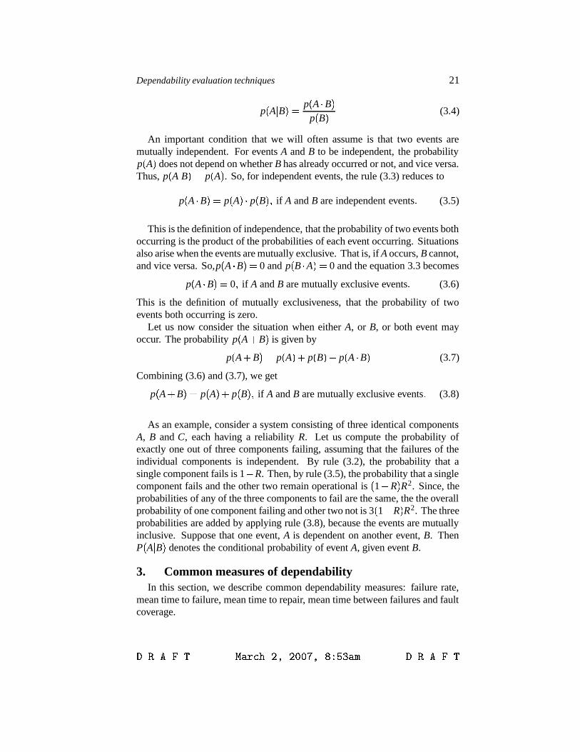
As an example, consider a system consisting of three identical componentsA, B and C, each having a reliability R. Let us compute the probability ofexactly one out of three components failing, assuming that the failures of theindividual components is independent. By rule (3.2), the probability that asingle component fails is 1 2 R. Then, by rule (3.5), the probability that a singlecomponent fails and the other two remain operational is % 1 2 R & R2. Since, theprobabilities of any of the three components to fail are the same, the the overallprobability of one component failing and other two not is 3 % 1 2 R & R2. The threeprobabilities are added by applying rule (3.8), because the events are mutuallyinclusive. Suppose that one event, A is dependent on another event, B. ThenP % A 3B & denotes the conditional probability of event A, given event B.
3. Common measures of dependabilityIn this section, we describe common dependability measures: failure rate,
mean time to failure, mean time to repair, mean time between failures and faultcoverage.
��������� � �����������������������! �"�$# ���������
22 FAULT TOLERANT DESIGN: AN INTRODUCTION
3.1 Failure rateFailure rate λ is the expected number of failures per unit time. For example,
if a processor fails, on average, once every 1000 hours, then it has a failure rateλ * 1 8 1000 failures/hour.
Often failure rate data is available at component level, but not for the entiresystem. This is because several professional organizations collect and publishfailure rate estimates for frequently used components (diodes, switches, gates,flip-flops, etc.). At the same time the design of a new system may involve newconfigurations of such standard components. When component failure rates areavailable, a crude estimation of the failure rate of a non-redundant system canbe done by adding the failure rates λi of the components:
λ * n
∑i 9 1
λi
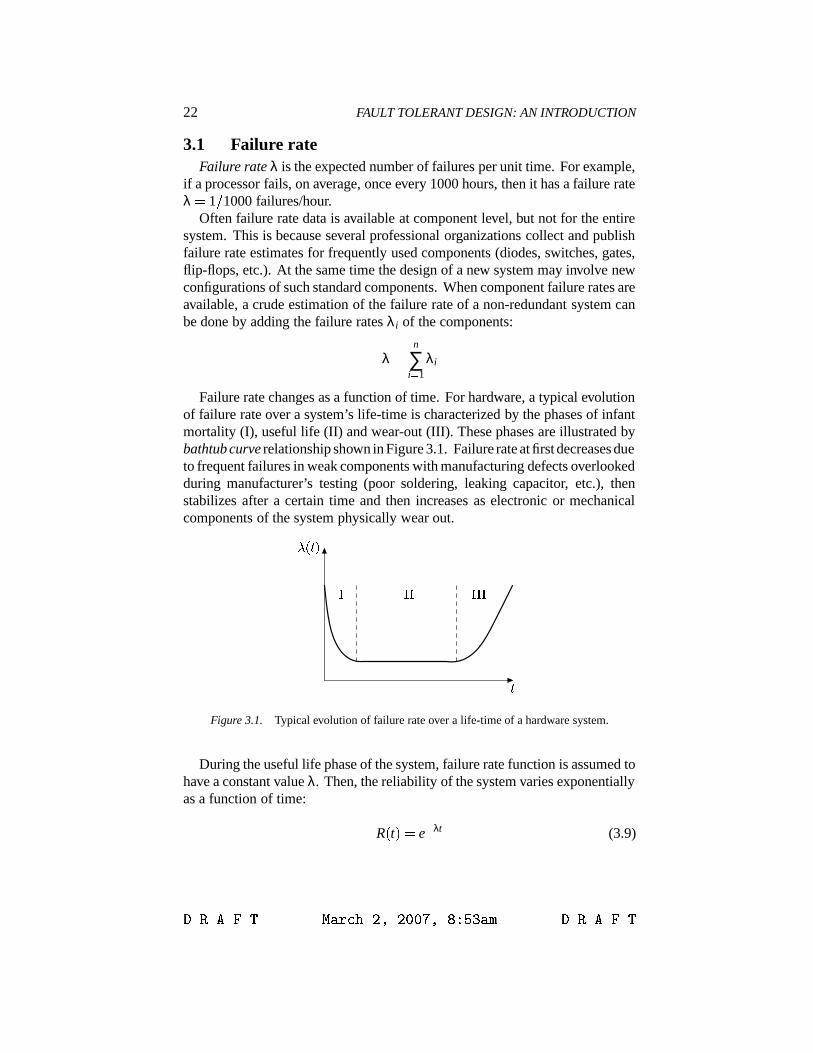
Failure rate changes as a function of time. For hardware, a typical evolutionof failure rate over a system’s life-time is characterized by the phases of infantmortality (I), useful life (II) and wear-out (III). These phases are illustrated bybathtub curve relationship shown in Figure 3.1. Failure rate at first decreases dueto frequent failures in weak components with manufacturing defects overlookedduring manufacturer’s testing (poor soldering, leaking capacitor, etc.), thenstabilizes after a certain time and then increases as electronic or mechanicalcomponents of the system physically wear out.
: :;: :;:<:=
>�? =<@
Figure 3.1. Typical evolution of failure rate over a life-time of a hardware system.
During the useful life phase of the system, failure rate function is assumed tohave a constant value λ. Then, the reliability of the system varies exponentiallyas a function of time:
R % t &+* e A λt (3.9)
��������� � �����������������������! �"�$# ���������

Dependability evaluation techniques 23
This law is known as exponential failure law. The plot of reliability as afunction of time is shown in Figure 3.2.
B
C
DFE >GHE >CIE > =
J ? =<@
Figure 3.2. Reliability plot R K t LNM e O λt .
The exponential failure law is very valuable for analysis of reliability ofcomponents and systems in hardware. However, it can only be used in caseswhen the assumption that the failure rate is constant is adequate. Softwarefailure rate usually decreases as a function of time. A possible curve is shownin Figure 3.3. The three phases of evolution are: test/debug (I), useful life (II)and obsolescence (III).
Software failure rate during useful life depends on the following factors:
1 software process used to develop the design and code
2 complexity of software,
3 size of software,
4 experience of the development team,
5 percentage of code reused from a previous stable project,
6 rigor and depth of testing at test/debug (I) phase.
There are two major differences between hardware and software curves.One difference is that, in the useful-life phase, software normally experiencesan increase in failure rate each time a feature upgrade is made. Since thefunctionality is enhanced by an upgrade, the complexity of software is likely tobe increased, increasing the probability of faults. After the increase in failure
��������� � �����������������������! �"�$# ���������

24 FAULT TOLERANT DESIGN: AN INTRODUCTION
rate due to an upgrade, the failure rate levels off gradually, partly because ofthe bugs found and fixed after the upgrades. The second difference is that, inthe last phase, software does not have an increasing failure rate as hardwaredoes. In this phase, the software is approaching obsolescence and there is nomotivation for more upgrades or changes.
: :;: :<:;:=
>�? =<@
Figure 3.3. Typical evolution of failure rate over a life-time of a software system.
3.2 Mean time to failureAnother important and frequently used measure of interest is mean time to
failure defined as follows.The mean time to failure (MTTF) of a system is the expected time until the
occurrence of the first system failure.If n identical systems are placed into operation at time t * 0 and the time t i,
i *QP 1 ( 2 (R-R-R-!( n S , that each system i operates before failing is measured then theaverage time is MTTF:
MTTF * 1n4 n
∑i 9 1
ti (3.10)
In terms of system reliability R % t & , MTTF is defined as
MTTF * , ∞
0R % t & dt - (3.11)
So, MTTF is the area under the reliability curve in Figure 3.2. If the reliabilityfunction obeys the exponential failure law (3.9), then the solution of (3.11) isgiven by
MTTF * 1λ
(3.12)
��������� � �����������������������! �"�$# ���������

Dependability evaluation techniques 25
where λ is the failure rate of the system. The smaller the failure rate is, thelonger is the time to the first failure.
In general, MTTF is meaningful only for systems that operate without repairuntil they experience a system failure. In a real situation, most of the missioncritical systems undergo a complete check-out before the next mission is under-taken. All failed redundant components are replaced and the system is returnedto a fully operational status. When evaluating the reliability of such systems,mission time rather than MTTF is used.
3.3 Mean time to repairThe mean time to repair (MTTR) of a system is the average time required to
repair the system.MTTR is commonly specified in terms for a repair rate µ, which is the
expected number of repairs per unit time:
MTTR * 1µ
(3.13)
MTTR depends on fault recovery mechanism used in the system, locationof the system, location of spare modules (on-cite versus off-cite), maintenanceschedule, etc. Low MTTR requirement means high operational cost of thesystem. For example, if repair is done by replacing the hardware module, thehardware spares are kept on-cite and the cite is maintained 24 hours a day, thenthe expected MTTR can be 30 min. However, if the cite maintenance is relaxedto regular working hours on week days only, the expected MTTR increases to3 days. If the system is remotely located and the operator need to be flown into replace the faulty module, the MTTR can be 2 weeks. In software, if thefailure is detected by watchdog timers and the processor automatically restartthe failed tasks, without operating system reboot, then MTTR can be 30 sec. Ifsoftware fault detection is not supported and a manual reboot by an operator isrequired, than MTTR can range from 30 min to 2 weeks, depending on locationof the system.
If the system experiences n failures during its lifetime, the total time that thesystem is operational is n 4 MTTF . Likewise, the total time the system is beingrepaired is n 4 MTTR. The steady state availability given by the expression (2.2)can be approximated as
A % ∞ &T* n 4 MTTFn 4 MTTF 5 n 4 MTTR
* MTTFMTTF 5 MTTR
(3.14)
In section 5.2.2, we will see an alternative approach for computing availability,which uses Markov processes.
��������� � �����������������������! �"�$# ���������

26 FAULT TOLERANT DESIGN: AN INTRODUCTION
3.4 Mean time between failuresThe mean time between failures (MTBF) of a system is the average time
between failures of the system.If we assume that a repair of the system makes the system a perfect one, then
the relationship between MTBF and MTTF is as follows:
MTBF * MTTF 5 MTT R (3.15)
3.5 Fault coverageThere are several types of fault coverage, depending on whether we are con-
cerned with fault detection, fault location, fault containment or fault recovery.Intuitively, fault coverage is the probability that the system will not fail to per-form the expected actions when a fault occurs. More precisely, fault coverageis defined in terms of the conditional probability P % A 3B & , read as “probabilityof A given B”.
Fault detection coverage is the conditional probability that, given the exis-tence of a fault, the system detects it.
C * P % fault detection 3 fault existence &For example, a system requirement can be that 99% of all single stuck-
at faults are detected. The fault detection coverage is a measure of system’sability to meet such a requirement.
Fault location coverage is the conditional probability that, given the existenceof a fault, the system locates it.
C * P % fault location 3 fault existence &It is common to require system to locate faults within easily replaceable
modules. In this case, the fault location coverage can be used as a measure ofsuccess.
Similarly, fault containment coverage is the conditional probability that,given the existence of a fault, the system contains it.
C * P % fault containment 3 fault existence &Finally, fault recovery coverage is the conditional probability that, given the
existence of a fault, the system recovers.
C * P % fault recovery 3 fault existence &��������� � �����������������������! �"�$# ���������

Dependability evaluation techniques 27
4. Dependability model typesIn this section we consider two common dependability models: reliability
block diagrams and Markov processes. Reliability block diagrams belong to aclass of combinatorial models, which assume that the failures of the individualcomponents are mutually independent. Markov processes belong to a classof stochastic processes which take the dependencies between the componentfailures into account, making the analysis of more complex scenarios possible.
4.1 Reliability block diagramsCombinatorial reliability models include reliability block diagrams, fault
trees, success trees and reliability graphs. In this section we will consider theoldest and most common reliability model: reliability block diagrams.
A reliability block diagram presents an abstract view of the system. Thecomponents are represented as blocks. The interconnections among the blocksshow the operational dependency between the components. Blocks are con-nected in series if all of them are necessary for the system to be operational.Blocks are connected in parallel if only one of them is sufficient for the systemto operate correctly. A diagram for a two-component serial system is shownin Figure 3.4(a). Figure 3.4(b) shows a diagram of a two-component parallelsystem. Models of more complex systems may be built by combining the serialand parallel reliability models.
UWVNXNY�Z\[ C UWVNXNY$Z][ G UWVNXNY�Z\[ CUWVNXNY�Z\[ GFigure 3.4. Reliability block diagram of a two-component system: (a) serial, (b) parallel.
As an example, consider a system consisting of two duplicated processorsand a memory. The reliability block diagram for this system is shown in Figure3.5. The processors are connected in parallel, since only one of them is sufficientfor the system to be operational. The memory is connected in series, since itsfailure would cause the system failure.
U^[`_aVcbedf�b;[Igh[Ii;i;Vcb Cf�b;VFi<[Ii;i;Vcb GFigure 3.5. Reliability block diagram of a three-component system.
��������� � �����������������������! �"�$# ���������

28 FAULT TOLERANT DESIGN: AN INTRODUCTION
Reliability block diagrams are a popular model, because they are easy tounderstand and to use for modeling systems with redundancy. In the nextsection we will see that they are also easy to evaluate using analytical methods.However, reliability block diagrams, as well as other combinatorial reliabilitymodels, have a number of serious limitations.
First, reliability block diagrams assume that the system components are lim-ited to the operational and failed states and that the system configuration doesnot change during the mission. Hence, they cannot model standby components,repair as well as complex fault detection and recovery mechanisms. Second, thefailures of the individual components are assumed to be independent. There-fore, the case when the sequence of component failures affects system reliabilitycannot be adequately represented.
4.2 Markov processesContrary to combinatorial models, Markov processes take into account the
interactions of component failures making the analysis of complex scenariospossible. Markov processes theory derives its name from the Russian mathe-matician A. A. Markov (1856-1922), who pioneered a systematic investigationof describing random processes mathematically.
Markov processes are a special class of stochastic processes. The basicassumption is that the behavior of the system in each state is memoryless.The transition from the current state of the system is determined only by thepresent state and not by the previous state or the time at which it reached thepresent state. Before a transition occurs, the time spent in each state followsan exponential distribution. In dependability engineering, this assumption issatisfied if all events (failures, repairs, etc.) in each state occur with constantoccurrence rates.
Markov processes are classified based on state space and time space char-acteristics as shown in Table 3.1. In most dependability analysis applications,
State Space Time Space Common Model NameDiscrete Discrete Discrete Time Markov ChainsDiscrete Continuous Continuous Time Markov ChainsContinuous Discrete Continuous State, Discrete Time
Markov ProcessesContinuous Continuous Continuous State, Continuous Time
Markov Processes
Table 3.1. Four types of Markov processes.
��������� � �����������������������! �"�$# ���������

Dependability evaluation techniques 29
the state space is discrete. For example, a system might have two states: op-erational and failed. The time scale is usually continuous, which means thatcomponent failure and repair times are random variables. Thus, ContinuousTime Markov Chains are the most commonly used. In some textbooks, they arecalled Continuous Markov Models. There are, however, applications in whichtime scale is discrete. Examples include synchronous communication protocol,shifts in equipment operation, etc. If both time and state space are discrete, thenthe process is called Discrete Time Markov Chain.
Markov processes are illustrated graphically by state transition diagrams.A state transition diagram is a directed graph G *j% V ( E & , where V is the setof vertices representing system states and E is the set of edges representingsystem transitions. State transition diagram is a mathematical model which canbe used to represent a wide variety of processes, i.e. radioactive breakdown orchemical reaction. For dependability models, a state is defined to be a particularcombination of operating and failed components. For example, if we have asystem consisting of two components, than there are four different combinationsenumerated in Table 3.2, where O indicates an operational component and Findicates a failed component.
Component State1 2 NumberO O 1O F 2F O 3F F 4
Table 3.2. Markov states of a two-component system.
The state transitions reflect the changes which occur within the system state.For example, if a system with two identical component is in the state (11), andthe first module fails, then the system moves to the state (01). So, a Markovprocess represents possible chains of events which occur within a system. Inthe case of dependability analysis, these events are failures and repairs.
Each edge carries a label, reflecting the rate at which the state transitionsoccur. Depending on the modeling goals, this can be failure rate, repair rate orboth.
We illustrate the concept first on a simple system, consisting of a singlecomponent.
��������� � �����������������������! �"�$# ���������

30 FAULT TOLERANT DESIGN: AN INTRODUCTION
4.2.1 Single-component system
A single component has only two states: one operational (state 1) and onefailed (state 2). If no repair is allowed, there is a single, non-reversible transi-tion between the states, with a label λ corresponding to the failure rate of thecomponent (Figure 3.6). C G>
Figure 3.6. State transition diagram of a single-component system.
If repair is allowed, then a transition between the failed and the operationalstates is possible, with a repair rate µ (Figure 3.7). State diagrams incorporatingrepair are used in availability analysis.C G>kFigure 3.7. State transition diagram of a single-component system incorporating repair.
Next, suppose that we would like to distinguish between a failed-safe andfailed-unsafe states, as required in safety analysis. Let state 2 be a failed-safeand state 3 be a fail-unsafe states (Figure 3.8). The transition between the state1 and state 2 depends on both, component failure rate λ and the probability that,given the existence of a fault, the system succeeds in detecting it and taking thecorresponding actions to fail in a safe manner, i.e. on fault coverage C. Thetransition between the state 1 and the failed-unsafe state 3 depends on failurerate λ and the probability that a fault is not detected, i.e. 1 2 C.
C GD
>6l>�? C�m l @
Figure 3.8. State transition diagram of a single-component system for safety analysis.
4.2.2 Two-component system
A two-component system has four possible states, enumerated in Table 3.2.The changes of states are illustrated by a state transition diagram shown in
��������� � �����������������������! �"�$# ���������
Dependability evaluation techniques 31
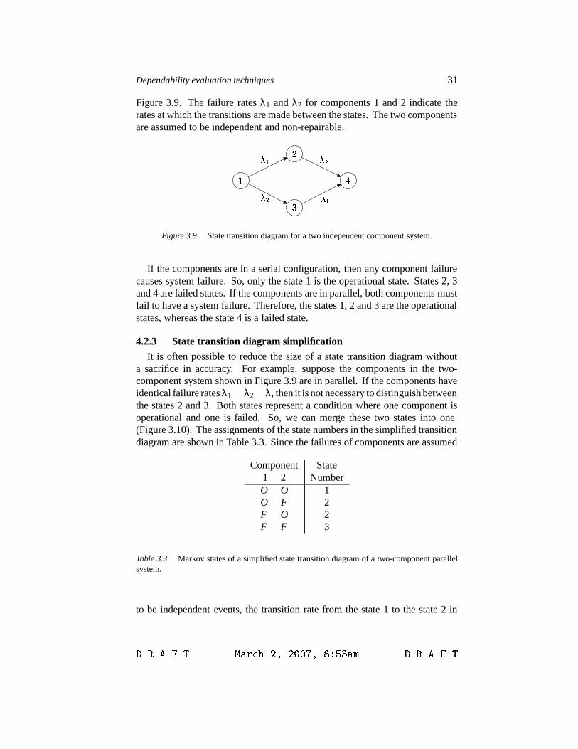
Figure 3.9. The failure rates λ1 and λ2 for components 1 and 2 indicate therates at which the transitions are made between the states. The two componentsare assumed to be independent and non-repairable.
C GD n>po
>7q>7q>po
Figure 3.9. State transition diagram for a two independent component system.
If the components are in a serial configuration, then any component failurecauses system failure. So, only the state 1 is the operational state. States 2, 3and 4 are failed states. If the components are in parallel, both components mustfail to have a system failure. Therefore, the states 1, 2 and 3 are the operationalstates, whereas the state 4 is a failed state.
4.2.3 State transition diagram simplification
It is often possible to reduce the size of a state transition diagram withouta sacrifice in accuracy. For example, suppose the components in the two-component system shown in Figure 3.9 are in parallel. If the components haveidentical failure rates λ1 * λ2 * λ, then it is not necessary to distinguish betweenthe states 2 and 3. Both states represent a condition where one component isoperational and one is failed. So, we can merge these two states into one.(Figure 3.10). The assignments of the state numbers in the simplified transitiondiagram are shown in Table 3.3. Since the failures of components are assumed
Component State1 2 NumberO O 1O F 2F O 2F F 3
Table 3.3. Markov states of a simplified state transition diagram of a two-component parallelsystem.
to be independent events, the transition rate from the state 1 to the state 2 in
��������� � �����������������������! �"�$# ���������

32 FAULT TOLERANT DESIGN: AN INTRODUCTION
Figure 3.10 is the sum of the transition rates from the state 1 to the states 2 and3 in Figure 3.9, i. e. 2λ. C G DG > >Figure 3.10. Simplified state transition diagram of a two-component parallel system.
5. Dependability computation methodsIn this section we study how reliability block diagrams and Markov processes
can be used to evaluate system dependability.
5.1 Computation using reliability block diagramsReliability block diagrams can be used to compute system reliability as well
as system availability.
5.1.1 Reliability computation
To compute the reliability of a system represented by a reliability blockdiagram, we need first to break the system down into its serial and parallelparts. Next, the reliabilities of these parts are computed. Finally, the overallsolution is composed from the reliabilities of the parts.
Given a system consisting of n components with Ri % t & being the reliabilityof the ith component, the reliability of the overall system is given by
R % t &T*sr ∏ni 9 1 Ri % t & for a series structure,
1 2 ∏ni 9 1 % 1 2 Ri % t &R& for a parallel structure.
(3.16)
In a serial system, all components should be operational for a system tofunction correctly. Hence, by rule (3.5), Rserial % t &1* ∏n
i 9 1 Ri % t & . In a parallelsystem, only one of the components is required for a system to be operational.So, the unreliability of a parallel system equals to the probability that all nelements fail, i.e. Qparallel % t &t* ∏n
i 9 1 Qi % t &t* ∏ni 9 1 % 1 2 Ri % t &R& . Hence, by rule
1, Rparallel % t &+* 1 2 Qparallel % t &T* 1 2 ∏ni 9 1 % 1 2 Ri % t &R& .
Designing a reliable serial system is difficult. For example, if a serial systemwith 100 components is to be build, and each of the components has a reliability0 - 999, the overall system reliability is 0 - 999100 * 0 - 905.
On the other hand, a parallel system can be made reliable despite the un-reliability of its component parts. For example, a parallel system of fouridentical modules with the module reliability 0.95, has the system reliabil-
��������� � �����������������������! �"�$# ���������

Dependability evaluation techniques 33
ity 1 2u% 1 2v- 95 & 4 * 0 - 99999375. Clearly, however, the cost of the parallelismcan be high.
5.1.2 Availability computation
If we assume that the failure and repair times are independent, then wecan use reliability block diagrams to compute the system availability. Thissituation occurs when the system has enough spare resources to repair all thefailed components simultaneously. Given a system consisting of n componentswith Ai % t & being the availability of the ith component, the availability if theoverall system is given by
A % t &T* r ∏ni 9 1 Ai % t & for a series structure,
1 2 ∏ni 9 1 % 1 2 Ai % t &R& for a parallel structure.
(3.17)
The combined availability of two components in series is always lower thanthe availability of the individual components. For example, if one componenthas the availability 99% (3.65 days/year downtime) and another componenthas the availability 99.99% (52 minutes/year downtime), then the availabilityof the system consisting of these two components in serial is 98.99% (3.69days/year downtime). Contrary, a parallel system consisting of three identicalcomponents with the individual availability 99% has availability 99.9999 (31seconds/year downtime).
5.2 Computation using Markov processesIn this section we show how Markov processes are used to evaluate system
dependability. Continuous Time Markov Chains are the most important classof Markov processes for dependability analysis, so the presentation is focusedon this model.
The aim of Markov processes analysis is to calculate Pi % t & , the probabilitythat the system is in the state i at time t. Once this is known, the systemreliability, availability or safety can be computed as a sum taken over all theoperating states.
Let us designate the state 1 as the state in which all the components areoperational. Assuming that at t * 0 the system is in state 1, we get
P1 % 0 &T* 1 -Since at any time the system can be only in one state, Pi % 0 &+* 0 (xw i y* 1, and wehave
∑i z O { F
Pi % t &T* 1 ( (3.18)
where the sum is over all possible states.
��������� � �����������������������! �"�$# ���������
34 FAULT TOLERANT DESIGN: AN INTRODUCTION
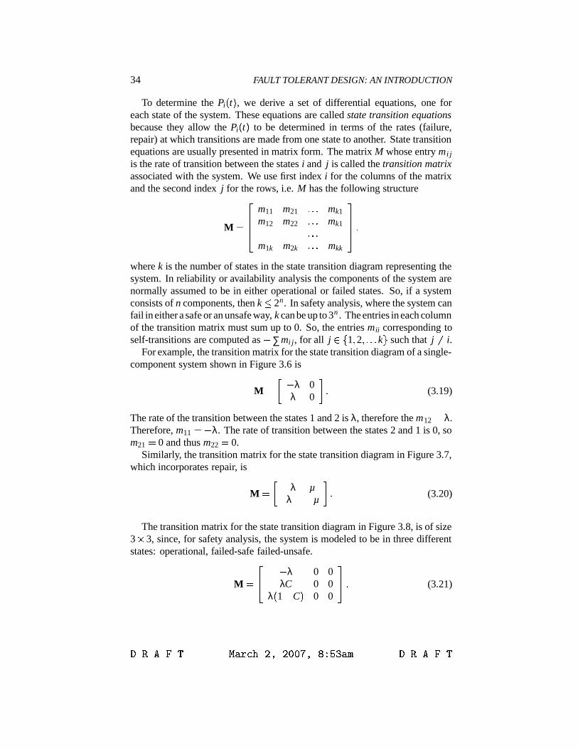
To determine the Pi % t & , we derive a set of differential equations, one foreach state of the system. These equations are called state transition equationsbecause they allow the Pi % t & to be determined in terms of the rates (failure,repair) at which transitions are made from one state to another. State transitionequations are usually presented in matrix form. The matrix M whose entry m i j
is the rate of transition between the states i and j is called the transition matrixassociated with the system. We use first index i for the columns of the matrixand the second index j for the rows, i.e. M has the following structure
M *}|~~� m11 m21 -R-R- mk1
m12 m22 -R-R- mk1-R-R-m1k m2k -R-R- mkk
�\��� -where k is the number of states in the state transition diagram representing thesystem. In reliability or availability analysis the components of the system arenormally assumed to be in either operational or failed states. So, if a systemconsists of n components, then k 0 2n. In safety analysis, where the system canfail in either a safe or an unsafe way, k can be up to 3n . The entries in each columnof the transition matrix must sum up to 0. So, the entries mii corresponding toself-transitions are computed as 2 ∑mi j, for all j ��P 1 ( 2 (R-R-R- k S such that j y* i.
For example, the transition matrix for the state transition diagram of a single-component system shown in Figure 3.6 is
M *�� 2 λ 0λ 0 � - (3.19)
The rate of the transition between the states 1 and 2 is λ, therefore the m12 * λ.Therefore, m11 *�2 λ. The rate of transition between the states 2 and 1 is 0, som21 * 0 and thus m22 * 0.
Similarly, the transition matrix for the state transition diagram in Figure 3.7,which incorporates repair, is
M * � 2 λ µλ 2 µ � - (3.20)
The transition matrix for the state transition diagram in Figure 3.8, is of size3 � 3, since, for safety analysis, the system is modeled to be in three differentstates: operational, failed-safe failed-unsafe.
M * |� 2 λ 0 0λC 0 0
λ % 1 2 C & 0 0
�� - (3.21)
��������� � �����������������������! �"�$# ���������

Dependability evaluation techniques 35
The transition matrix for the simplified state transition diagram of the two-component system, shown in Figure 3.10 is
M * |� 2 2λ 0 02λ 2 λ 00 λ 0
�� - (3.22)
The examples above illustrate two important properties of transition matrices.One, which we have mentioned before, is that the sum of the entries in eachcolumn is zero. Positive sign of an i jthe entry indicates that the transitionoriginates in the ith state. Negative sign of an i jthe entry indicates that thetransition terminates in the ith state.
Second property of the transition matrix is that it allows us to distinguishbetween the operational and failed states. In reliability analysis, once a systemfailed, a failed state cannot be leaved. Therefore, each failed state i has a zerodiagonal element mii. This is not the case, however, when availability or safetyare computed, as one can see from (3.20) and (3.21).
Using state transition matrices, state transition equations are derived as fol-lows. Let P % t & be a vector whose ith element is the probability Pi % t & that thesystem is in state i at time t. Then the matrix representation of a system of statetransition equations is given by
ddt
P % t &+* M 4 P % t &!- (3.23)
Once the system of equations is solved and the Pi % t & are known, the systemreliability, availability or safety can be computed as a sum taken over all theoperating states.
We illustrate the computation process on a number of simple examples.
5.2.1 Reliability evaluation
Independent components caseLet us first compute reliability of a parallel system consisting of two inde-
pendent components which we have considered before (Figure 3.9). Applying(3.23) to the the matrix (3.22) we get
ddt |� P1 % t &
P2 % t &P3 % t &
�� * |� 2 2λ 0 02λ 2 λ 00 λ 0
�� 4 |� P1 % t &P2 % t &P3 % t &
�� -The above matrix form represents the following system of state transition equa-tions ���� ��� d
dt P1 % t &�*�2 2λP1 % t &ddt P2 % t &�* 2λP1 % t &�2 λP2 % t &ddt P3 % t &�* λP2 % t &
��������� � �����������������������! �"�$# ���������

36 FAULT TOLERANT DESIGN: AN INTRODUCTION
By solving this system of equations, we get
P1 % t &T* e A 2λt
P2 % t &T* 2e A λt 2 2e A 2λt
P3 % t &T* 1 2 2e A λt 5 e A 2λt
Since the Pi % t & are known, we can now calculate the reliability of the system.For the parallel configuration, both components should fail to have a systemfailure. Therefore, the reliability of the system is the sum of probabilities P1 % t &and P2 % t & :
Rparallel % t &�* 2e A λt 2 e A 2λt (3.24)
In general case, the reliability of the system is computed as a function using theequation
R % t &T* ∑i z O
Pi % t &!( (3.25)
where the sum is taken over all the operating states O. Alternatively, the relia-bility can be calculated
R % t &T* 1 2 ∑i z F
Pi % t &!(where the sum is taken over all the states F in which the system has failed.
Note that, for constant failure rates, the component reliability is R % t &�* e A λt .Therefore, the equation (3.24) can be written as Rparallel % t &t* 2R2 2 R, whichagrees with the expression (3.16) derived using reliability block diagrams. Tworesults are the same, because in this example we assumed the failure rates to bemutually independent.
Dependant components caseThe value of Markov processes become evident in situations in which com-
ponent failure rates are no longer assumed to be independent of the system state.One of the common cases of dependence is load-sharing components, whichwe consider next. Another possibility is the case of standby components, whichis considered in the availability computation section.
The word load is used in a broad sense of the stress on a system. This can bean electrical load, a load caused by high temperature, or an information load.On practice, failure rates are found to increase with loading. Suppose that twocomponents share a load. If one of the component fails, the additional load onthe second component is likely to increase its failure rate.
To model load-sharing failures, consider the state transition diagram of atwo-component parallel system shown in Figure 3.11. As before, we have fourstates. However, after one component failure, the failure rate of the secondcomponent increases. The increased failure rates of the components 1 and 2are denoted with λ �1 and λ �2, respectively.
��������� � �����������������������! �"�$# ���������

Dependability evaluation techniques 37
C GD n>po
>7q>7�q>7�o
Figure 3.11. State transition diagram of a two-component parallel system with load sharing.
From the state transition diagram in Figure 3.11, we can derive the statetransition equations for Pi % t & . In the matrix form they are
ddt
|~~� P1 % t &P2 % t &P3 % t &P4 % t &
�\��� * |~~� 2 λ1 2 λ2 0 0 0λ1 2 λ �2 0 0λ2 0 2 λ �1 00 λ �2 λ �1 0
�\��� 4 |~~� P1 % t &P2 % t &P3 % t &P4 % t &
�\��� -By expanding the matrix form, we get the following system of equations������� ������
ddt P1 % t &T*�%�2 λ1 2 λ2 & P1 % t &ddt P2 % t &T* λ1P1 % t &�2 λ �2P2 % t &ddt P3 % t &T* λ2P1 % t &�2 λ �1P3 % t &ddt P4 % t &T* λ �2P2 % t &65 λ �1P3 % t &!-
The solution of this system of equation is
P1 % t &T* e . A λ1 A λ2 � tP2 % t &T* λ1
λ1 � λ2 A λ �2 eλ �2t 2 λ1λ1 � λ2 A λ �2 e . A λ1 A λ2 � t
P3 % t &T* λ2λ1 � λ2 A λ �1 eλ �1t 2 λ2
λ1 � λ2 A λ �1 e . A λ1 A λ2 � tP4 % t &T* 1 2 e . A λ1 A λ2 � t 2 λ1
λ1 � λ2 A λ �2 eλ �2t 5 λ1λ1 � λ2 A λ �2 e . A λ1 A λ2 � t2 λ2
λ1 � λ2 A λ �1 eλ �1t 5 λ2λ1 � λ2 A λ �1 e . A λ1 A λ2 � t -
Finally, since both components should fail for the system to fail, the reliabilityis equal to 1 2 P4 % t & , yielding the expression
Rparallel % t &T* e . A λ1 A λ2 � t 5 λ1λ1 � λ2 A λ �2 eλ �2t 2 λ1
λ1 � λ2 A λ �2 e . A λ1 A λ2 � t5 λ2λ1 � λ2 A λ �1 eλ �1t 2 λ2
λ1 � λ2 A λ �1 e . A λ1 A λ2 � t - (3.26)
��������� � �����������������������! �"�$# ���������

38 FAULT TOLERANT DESIGN: AN INTRODUCTION
If λ �1 * λ1 and λ �2 * λ2, the above equation is equal to (3.24). The effect of theincreased loading can be illustrated as follows. Assume that the two componentsare identical, i.e. λ1 * λ2 * λ and λ �1 * λ �2 * λ � . Then, the equation (3.26)reduces to
Rparallel % t &T* 2λ2λ 2 λ � e A λ � t 2 λ �
2λ 2 λ � e A 2λt -
B DGC
C
> �7���> �7� >> �7� G >i<�\���cZ\[�ghVH_��6Vc�$[`�H�
> =
J��¡ `�£¢¥¤§¦
Figure 3.12. Reliability of a two-component parallel system with load sharing.
Figure 3.12 shows the reliability of a two-component parallel system withload-sharing for different values of λ � . The reliability e A λt of a single-componentsystem is also plotted for a comparison. In case of λ �¨* λ two components areindependent, so the reliability is given by (3.23). λ �p* ∞ is the case of totaldependency. The failure of one component brings an immediate failure of an-other component. So, the reliability equals to the reliability of a serial systemwith two components (3.16). It can been seen that, the more the values of λ �exceeds the value of λ, the closer the reliability of the system approaches serialsystem with two components reliability.
5.2.2 Availability evaluation
In availability analysis, as well as in reliability analysis, there are situa-tions in which the component failures cannot be considered independent of oneanother. These include shared-load systems and systems with standby compo-nents, which are repairable.
The dependencies between component failures can be analyzed using Markovmethods, provided that the failures are detected and that the failure and repairrates are time-independent. There is a fundamental difference between treat-
��������� � �����������������������! �"�$# ���������

Dependability evaluation techniques 39
ment of repair for reliability and availability analysis. In reliability calculations,components are allowed to be repaired only as long as the system has not failed.In availability calculations, the components can also be repaired after the systemfailure.
The difference is best illustrated on a simple example of a system with twocomponents, one primary and one standby. The standby component is held inreserve and only brought to operation when the primary component fails. Weassume that there is a perfect fault detection unit which detects a failure in theprimary component and replace it by the standby component. We also assumethat the standby component cannot fail while it is in the standby mode.
The state transition diagrams of the standby system for reliability and avail-ability analysis are shown in Figure 3.13(a) and (b), respectively. The states arenumbered according to the Table 3.4. When the primary component fails, there
Component State1 2 NumberO O 1F O 2F F 3
Table 3.4. Markov states of a simplified state transition diagram of a two-component parallelsystem incorporating repair.
is a transition between the states 1 and 2. If a system is in the state 2 and thebackup component fails, there is a transition to the state 3. Since we assumedthat the backup unit cannot fail while in the standby mode, the combination% O ( F & cannot occur. The states 1 and 2 are operational states. The state 3 isthe failed state.C G D C G D>po
k > q >pok
>pok?¥© @ ?«ª @
Figure 3.13. Sate transition diagrams for a standby two-component system (a) for reliabilityanalysis, (b) for availability analysis.
Suppose the primary unit can be repaired with a rate µ. For reliability anal-ysis, this implies that a transition between the states 2 and 1 is possible. The
��������� � �����������������������! �"�$# ���������

40 FAULT TOLERANT DESIGN: AN INTRODUCTION
corresponding transition matrix if given by
M * |� 2 λ1 µ 0λ1 2 λ2 2 µ 00 λ2 0
�� -For availability analysis, we should be able to repair the backup unit as well.This adds a transition between the states 3 and 2. We assume that the repair ratesfor primary and backup units are the same. We also assume that the backupunit will be repaired first. The corresponding transition matrix if given by
M * |� 2 λ1 µ 0λ1 2 λ2 2 µ µ0 λ2 2 µ
�� - (3.27)
One can see that, in the matrix for availability calculations, none of thediagonal elements is zero. This is because the system should be able to recoverfrom the failed state. By solving the system of state transition equations, wecan get Pi % t & and compute the availability of the system as
A % t &T* 1 2 ∑i z F
Pi % t &!( (3.28)
where the sum is taken over all the failed states F .Usually, the steady state availability rather than the time dependent avail-
ability is of interest. The steady state availability can be computed in a simplerway. We note that, as time approach infinity, the derivative on the right-handside of the equation 3.23 vanishes and we get a time-independent relationship
M 4 P % ∞ &+* 0 - (3.29)
In our example, for matrix (3.27) this represents a system of equations���� ��� 2 λ1P1 % ∞ &65 µP2 % ∞ &T* 0
λ1P1 % ∞ &�2u% λ2 5 µ & P2 % ∞ &75 µP3 % ∞ &T* 0
λ2P2 % ∞ &�2 µP3 % ∞ &+* 0
Since these three equations are linearly dependent, they are not sufficient tosolve for P % ∞ & . The needed piece of additional information is the condition(3.18) that the sum of all probabilities is one:
∑i
Pi % ∞ &T* 1 - (3.30)
��������� � �����������������������! �"�$# ���������

Dependability evaluation techniques 41
If we assume λ1 * λ2 * λ, then we get
P1 % ∞ &T*�¬ 1 5 λµ 5% λ
µ & 2 ® A 1 (P2 % ∞ &T* ¬ 1 5 λ
µ 5% λµ & 2 ® A 1 λ
µ (P3 % ∞ &T*�¬ 1 5 λ
µ 5% λµ & 2 ® A 1 ¯ λ
µ ° 2 -The steady-state availability can be found by setting t * ∞ in (3.28)
A % ∞ &+* 1 2 � 1 5 λµ5�% λ
µ& 2 � A 1 ± λ
µ ² 2 -If we further assume that λ 8 µ ³´³ 1, we can write
A % ∞ &+µ 1 2 ± λµ ² 2 -
To summarize, steady-state availability problems are solved by the same pro-cedure as time-dependent availability. Any n 2 1 of the n equations representedby (3.29) are combined with the condition 3.30 to solve for the components ofP % ∞ & . These are then substituted into (3.28) to obtain availability.
5.2.3 Safety evaluation
The main difference between safety calculation and reliability calculation isin the construction of the state transition diagram. As we mentioned before,for safety analysis, the failed state is splitted into failed-safe and failed-unsafeones. Once the state transition diagram for a system is derived, the state transi-tion equations are obtained and solved using same procedure as for reliabilityanalysis.
As an example, consider the single component system shown in Figure 3.8.Its state transition matrix is given by (3.21). So, the state transition equationsfor Pi % t & are given by
ddt |� P1 % t &
P2 % t &P3 % t &
�� * |� 2 λ 0 0λC 0 0
λ % 1 2 C & 0 0
�� 4 |� P1 % t &P2 % t &P3 % t &
�� -The solution of this system of equations is
P1 % t &�* e A λt
P2 % t &�* C 2 Ce A λt
P3 % t &�*�% 1 2 C &�2u% 1 2 C & e A λt
��������� � �����������������������! �"�$# ���������

42 FAULT TOLERANT DESIGN: AN INTRODUCTION
The safety of the system is the sum of probabilities of being in the operationalor fail-safe states, i.e.
S % t &�* P1 % t &65 P2 % t &T* C 5% 1 2 C & e A λt
At time t * 0 the safety of the system is 1, as expected. As time approachesinfinity, the safety approaches the fault detection coverage, S % 0 &¶* C. So, ifC * 1, the system has a perfect safety.
6. Problems3.1. Why is dependability evaluation important?
3.2. What is the difference between qualitative and quantitative evaluation?
3.3. Define the failure rate. How the failure rate of a non-redundant system canbe computed from the failure rates of its components?
3.4. How does a typical evolution of failure rate over a system’s life-time differfor hardware and software?
3.5. What is the mean time to failure of a system? How can the MTTF of anon-redundant system be computed from the MTTF of its components?
3.6. What is the difference between the mean time to repair and the mean timebetween failures?
3.7. A heart pace-maker has a constant failure rate of λ * 8 - 167 8 109 hr.
(a) What is the probability that it will fail during the first year of operation?
(b) What is the probability that it will fail within 5 years of operation?
(b) What is the MTTF?
3.8. A logic circuit with no redundancy consists of 16 two-input NAND gatesand 3 J-K flip-flops. Assuming the constant failure rates of a two-inputNAND gate and a J-K flip-flop are 0.2107 and 0.4667 per hour, respectively,compute
(a) the failure rate of the logic circuit,
(b) the reliability for a 72-hour mission,
(c) the MTTF.
3.9. An automatic teller machine manufacturer determines that his product hasa constant failure rate of λ * 77 - 16 per 106 hours in normal use. For howlong should the warranty be set if no more than 5% of the machines are tobe returned to the manufacturer for repair?
��������� � �����������������������! �"�$# ���������

Dependability evaluation techniques 43
3.10. A car manufacturer estimates that the reliability of his product is 99% duringthe first 7 years.
(a) How many cars will need a repair during the first year?
(b) What is the MTTF?
3.11. A two-year guarantee is given on a TV-set based on the assumption that nomore than 3% of the items will be returned for repair. Assuming exponentialfailure law, what is the maximum failure rate that can be tolerated?
3.12. A DVD-player manufacturer determines that the average DVD set is used930 hr/year. A two-year warranty is offered on the DVD set having MTTFof 2500 hr. If the exponential failure law holds, which fraction of DVD-setswill fail during the warranty period?
3.13. Suppose the failure rate of a jet engine is λ * 10 A 3 per hour. What is theprobability that more than two engines on a four-engine aircraft will failduring a 4-hour flight? Assume that the failures are independent.
3.14. A non-redundant system with 50 components has a design life reliability of0 - 95. The system is re-designed so that it has only 35 components. Estimatethe design life reliability of the re-designed system. Assume that all thecomponents have constant failure rate of the same value and the failures areindependent.
3.15. At the end of the year of service the reliability of a component with a constantfailure rate is 0.96.
(a) What is the failure rate?
(b) If two components are put in parallel, what is the one year reliability?Assume that the failures are independent.
3.16. A lamp has three 25V bulbs. The failure rate of a bulb is λ * 10 A 3 per year.What is the probability that more than one bulb fail during the first month?
3.17. Suppose a component has a failure rate of λ * 0 - 007 per hour. How manycomponents should be placed in parallel if the system is to run for 200 hourswith failure probability of no more than 0.02? Assume that the failures areindependent.
3.18. Consider a system with three identical components with failure rate λ. Findthe system failure rate λsys for the following cases:
(a) All three components in series.
(b) All three components in parallel.
��������� � �����������������������! �"�$# ���������

44 FAULT TOLERANT DESIGN: AN INTRODUCTION
(c) Two components in parallel and the third in series.
3.19. The MTTF of a system with constant failure rate has been determined tobe 1000 hr. An engineer is to set the design life time so that the end-of-lifereliability is 0.95.
(a) Determine the design life time.
(b) If two systems are placed in parallel, to what value may the design lifetime be increased without decreasing the end-of-life reliability?
3.20. A printer has an MTTF = 168 hr and MTTR = 3 hr.
(a) What is the steady state availability?
(b) If MTTR is reduced to 1 hr, what MTTF can be tolerated without de-creasing the availability of the printer?
3.21. A copy machine has a failure rate of 0.01 per week. What repair rate shouldbe maintained to achieve a steady state availability of 95%?
3.22. Suppose that the steady state availability for standby system should be 0.9.What is the maximum acceptable value of the failure to repair ratio λ 8 µ?
3.23. A computer system is designed to have a failure rate of one fault in 5 years.The rate remains constant over the life of the system. The system has nofault-tolerance capabilities, so it fails upon occurrence of the first fault. Forsuch a system:
(a) What is the MTTF?
(b) What is the probability that the system will fail in its first year of oper-ation?
(c) The vendor of this system wishes to offer insurance against failure forthe three years of operation of the system at some extra cost. The vendordetermined that it should charge $200 for each 10% drop in reliabilityto offer such an insurance. How much should the vendor charge to theclient for such an insurance?
3.24. What are the basic assumptions regarding the failures of the individual com-ponents (a) in reliability block diagram model; (b) in Markov process model?
3.25. A system consists of three modules: M1 ( M2 and M3. It was analyzed, andthe following reliability expression was derived:
Rsystem * R1R3 5 R2R3 2 R1R2R3
Draw the reliability block diagram for this system.
��������� � �����������������������! �"�$# ���������

Dependability evaluation techniques 45
3.26. A system with four modules: A ( B ( C and D is connected so that it operatescorrectly only if one of the two conditions is satisfied:
modules A and D operate correctly,
module A operates correctly and either B or C operates correctly.
Answer the following questions:
(a) Draw the reliability block diagram of the above system such that everymodule appears only once.
(b) What is the reliability of the system? Assume that the reliability of themodule X is R % X & and that the modules fail independently from eachother.
(c) What is the reliability of the above system as a function of time t, ifthe failure rates of the components are λA * λB * λC * λD * 0 - 01 peryear? Assume that the exponential failure law holds.
3.27. How many states has a non-simplified state transition diagram of a systemconsisting of n components? Assume that every component has only twostates: operational and failed.
3.28. Construct the Markov model of the three-component system shown in Figure3.5. Assume that the components are independent and non-repairable. Thefailure rate of the processors 1 and 2 is λp. The failure rates of the memoryis λm. Derive and solve the system of state transition equations representingthis system. Compute the reliability of the system.
3.29. Construct the Markov model of the three-component system shown in Figure3.5 for the case when a failed processor can be repaired. Assume that thecomponents are independent and that a processor can be repaired as long asthe system has not failed. The failure rate of the processors 1 and 2 is λ p.The failure rate of the memory is λm. Derive and solve the system of statetransition equations representing this system. Compute the reliability of thesystem.
3.30. What is the difference between treatment of repair for reliability and avail-ability analysis?
3.31. Construct the Markov model of the three-component system shown in Figure3.5 for availability analysis. Assume that the components are independentand that the processors and the memory can be repaired after the systemfailure. The failure rate of the processors 1 and 2 is λp. The failure rate ofthe memory is λm. Derive and solve the system of state transition equationsrepresenting this system. Compute the reliability of the system.
��������� � �����������������������! �"�$# ���������

46 FAULT TOLERANT DESIGN: AN INTRODUCTION
3.32. Suppose that the reliability of a system consisting of 4 blocks, two of whichare identical, is given by the following equation:
Rsystem * R1R2R3 5 R21 2 R2
1R2R3
Draw the reliability block diagram representing the system.
3.33. Construct a Markov chain and write a transition matrix for self-purgingredundancy with 3 modules, for the cases listed below. For all cases, assumethat the component’s failures are independent events and that the failure rateof each module is λ. For all cases, simplify state transition diagrams asmuch as you can.
(a) Do reliability evaluation, assuming that the voter and switches are per-fect and no repairs are allowed.
(b) Do reliability evaluation, assuming that the voter can fail with the failurerate λv, the switches are perfect, and no repairs are allowed.
(c) Do reliability evaluation, assuming that the voter and switches are per-fect and repairs are allowed. Assume that each module has its ownrepair crew (i.e. that the component’s repairs are independent events)and that the repair rate of each module is µ.
(d) Do availability evaluation, assuming that the voter and switches areperfect and repairs are allowed. Assume that there is a single repaircrew for all modules that can handle only one module at a time and thatthe repair rate of each module is µ.
��������� � �����������������������! �"�$# ���������

Chapter 4
HARDWARE REDUNDANCY
Those parts of the system that you can hit with a hammer (not advised) are called hardware;those program instructions that you can only curse at are called software.
—Anonymous
1. IntroductionHardware redundancy is achieved by providing two or more physical in-
stances of a hardware component. For example, a system can include redundantprocessors, memories, buses or power supplies. Hardware redundancy is oftenthe only available method for improving dependability of a system, when othertechniques, such as better components, design simplification, manufacturingquality control, software debugging, have been exhausted or shown to be morecostly than redundancy.
Originally, hardware redundancy techniques were used to cope with low reli-ability of individual hardware elements. Designers of early computing systemsreplicated components at gate and flip-flop levels and used comparison or vot-ing to detect or correct faults. As reliability of hardware components improved,the redundancy was shifted at the level of larger components, such as wholememories or arithmetic unit, thus reducing the relative complexity of the voteror comparator with respect to that of redundant units.
There are three basic forms of hardware redundancy: passive, active andhybrid. Passive redundancy achieves fault tolerance by masking the faults thatoccur without requiring any action on the part of the system or an operator.Active redundancy requires a fault to be detected before it can be tolerated.After the detection of the fault, the actions of location, containment and recov-ery are performed to remove the faulty component from the system. Hybridredundancy combine passive and active approaches. Fault masking is used to
��������� � �����������������������! �"�$# ���������

48 FAULT TOLERANT DESIGN: AN INTRODUCTION
prevent generation of erroneous results. Fault detection, location and recoveryare used to replace the faulty component with a spare component.
Hardware redundancy brings a number of penalties: increase in weight,size, power consumption, as well as time to design, fabricate, and test. Anumber of choices need to be examined to determine a best way to incorporateredundancy to the system. For example, weight increase can be reduced byapplying redundancy to the lower-level components. Cost increase can beminimized if the expected improvement in dependability reduces the cost ofpreventive maintenance for the system. In this section, we examine a numberof different redundancy configurations and calculate the effect of redundancy onsystem dependability. We also discuss the problem of common-mode failureswhich are caused by faults occurring in a part of the system common to allredundant components.
2. Redundancy allocationThe use of redundancy does not immediately guarantee an improvement in
the dependability of a system. The increase in weight, size and power consump-tion caused by redundancy can be quite severe. The increase in complexity maydiminish the dependability improvement, unless a careful analysis is performedto show that a more dependable system can be obtained by allocating the re-dundant resources in a proper way.
A number of possibilities have to be examined to determine at which levelredundancy needs to be provided and which components need to be made re-dundant. To understand the importance of these decisions, consider a serialsystem consisting of two components with reliabilities R1 and R2. If the systemreliability R * R1R2 does not satisfy the design requirements, the designer maydecide to make some of the components redundant. The possible choices ofredundant configurations are shown in Figure 4.1(a) and (b). Assuming thecomponent failures are mutually independent, the corresponding reliabilities ofthese systems are
Ra *�% 2R1 2 R21 & R2
Rb *�% 2R2 2 R22 & R1
GCC C GG?¥© @ ?«ª @Figure 4.1. Redundancy allocation.
��������� � �����������������������! �"�$# ���������

Hardware redundancy 49
Taking the difference of Rb and Ra, we get
Ra 2 Rb * R1R2 % R2 2 R1 &It follows from this expression that the higher reliability is achieved if weduplicate the component that is least reliable. If R1 ³ R2, then configurationFigure 4.1(a) is preferable, and vice versa.
Another important parameter to examine is the level of redundancy. Considerthe system consisting of three serial components. In high-level redundancy, theentire system in duplicated, as shown in Figure 4.2(a). In low-level redundancy,the duplication takes place at component level, as shown in Figure 4.2(b). Ifeach of the block of the diagram is a subsystem, the redundancy can be placedat even lower levels.CC GG DD CC GG DD?¥© @ ?¥ª @
Figure 4.2. High-level and low-level redundancy.
Let us compare the reliabilities of the systems in Figures 4.2(a) and (b).Assuming that the component failures are mutually independent, we have
Ra * 1 2u% 1 2 R1R2R3 & 2Rb *�% 1 2u% 1 2 R1 & 2 &·% 1 2u% 1 2 R2 & 2 &·% 1 2¸% 1 2 R3 & 2 &
The system in Figure 4.2(a) is a parallel combination of two serial sub-systems.The system in Figure 4.2(b) is a serial combination of three parallel sub-systems.As we can see, the reliabilities Ra and Rb differ, although the systems have thesame number of components. If RA * RB * RC, then the difference is
Rb 2 Ra * 6R3 % 1 2 R & 2Consequently, Rb ¹ Ra, i.e. low-level redundancy yields higher reliability thanhigh-level redundancy. However, this dependency only holds if the componentsfailures are truly independent in both configurations. In reality, common-modefailures are more likely to occur with low-level rather than with high-levelredundancy, since in high-level redundancy the redundant units are normallyisolated physically and therefore are less prone to common sources of stress.
3. Passive redundancyPassive redundancy approach masks faults rather than detect them. Masking
insures that only correct values are passed to the system output in spite of the
��������� � �����������������������! �"�$# ���������

50 FAULT TOLERANT DESIGN: AN INTRODUCTION
presence of a fault. In this section we first study a concept of triple modularredundancy, and then extend it to a more general case of N-modular redundancy.
3.1 Triple modular redundancyThe most common form of passive hardware redundancy is triple modular
redundancy (TMR). The basic configuration is shown in Figure 4.3. The com-ponents are triplicated to perform the same computation in parallel. Majorityvoting is used to determine the correct result. If one of the modules fails, themajority voter will mask the fault by recognizing as correct the result of theremaining two fault-free modules. Depending on the application, the triplicatedmodules can be processors, memories, disk drives, buses, network connections,power supplies, etc.
º+V»�e[`bUWVNXNY�Z\[ CUWVNXNY�Z\[ GUWVNXNY�Z\[ D�\����YN� C�\����YN� G�\����YN� D VcY��;��YN�
Figure 4.3. Triple modular redundancy.
A TMR system can mask only one module fault. A failure in either of theremaining modules would cause the voter to produce an erroneous result. InSection 5 we will show that the dependability of a TMR system can be improvedby removing failed modules from the system.
TMR is usually used in applications where a substantial increase in reliabilityis required for a short period. For example, TMR is used in the logic sectionof launch vehicle digital computer (LVDC) of Saturn 5. Saturn 5 is a rocketcarrying Apollo spacecrafts to the orbit. The functions of LVDC include themonitoring, testing and diagnosis of rocket systems to detect possible failures orunsafe conditions. As a result of using TMR, the reliability of the logic sectionfor a 250-hr mission is approximately twenty times larger than the reliabilityof an equivalent simplex system. However, as we see in the next section, forlonger duration missions, a TMR system is less reliable than a simplex system.
3.1.1 Reliability evaluation
The fact that a TMR system which can mask one module fault does notimmediately imply that the reliability of a TMR system is higher than thereliability of a simplex system. To estimate the influences of TMR on reliability,
��������� � �����������������������! �"�$# ���������

Hardware redundancy 51
we need to take the reliability of modules as well as the duration of the missioninto account.
A TMR system operates correctly as long as two modules operate correctly.Assuming that the voter is perfect and that the component failures are mutuallyindependent, the reliability of A TMR systems is given by
RTMR * R1R2R3 5% 1 2 R1 & R2R3 5 R1 % 1 2 R2 & R3 5 R1R2 % 1 2 R3 &The term R1R2R3 gives the probability that the first module functions correctlyand the second module functions correctly and the third module functions cor-rectly. The term % 1 2 R1 & R2R3 stands for the probability that the first modulehas failed and the second module functions correctly and the third module func-tions correctly, etc. The overall probability is an or of the probabilities of theterms since the events are mutually exclusive. If R1 * R2 * R3 * R, the aboveequation reduces to
RTMR * 3R2 2 2R3 (4.1)
Figure 4.4 compares the reliability of a TMR system RTMR to the reliabilityof a simplex system consisting of a single module with reliability R. The
B ¼¾½ C¼¾½C JJ�¿pÀ�Á
J�¦ÃÂeÄ�ÅIÆ]¤
J �§ `�£¢¥¤¡¦
Figure 4.4. TMR reliability compared to simplex system reliability.
reliabilities of the modules composing the TMR system are assumed to beequal R. As can be seen, there is a point at which RTMR * R. This point canbe found by solving the equation 3R2 2 2R3 * R. The three solutions are 0.5, 1and 0, implying that the reliability of a TMR system is equal to the reliabilityof a simplex system when the reliability of the module is R * 0 - 5, when themodule is perfect (R * 1), or when the module is failed (R * 0).
��������� � �����������������������! �"�$# ���������

52 FAULT TOLERANT DESIGN: AN INTRODUCTION
This further illustrates a difference between fault tolerance and reliability. Asystem can be fault-tolerant and still have a low overall reliability. For example,a TMR system build out of poor-quality modules with R * 0 - 2 will have a lowreliability of RTMR * 0 - 136. Vice versa, a system which cannot tolerate anyfaults can have a high reliability, e.g. when its components are highly reliable.However, such a system will fail as soon as the first fault occurs.
Next, let us consider how the reliability of a TMR system changes as afunction of time. For a constant failure rate λ, the reliability of the systemvaries exponentially as a function of time R % t &1* e A λt (3.9). Substituting thisexpression in (4.1), we get
RTMR % t &+* 3e A 2λt 2 2e A 3λt (4.2)
Figure 4.5 shows how the reliabilities of simplex and TMR systems changeas functions of time. The value of λt, rather than t is shown on the x-axis, to
B ¼ÈǼ ½C
DGC
JJ�¿pÀ�Á
> =
J��¡ `�£¢¥¤§¦
Figure 4.5. TMR reliability as a function of λt.
make the comparison independent of the failure rate. Recall that 1 8 λ * MTTF(3.12), so that the point λt * 1 corresponds to the time when the system isexpected to experience the first failure. One can see that reliability of TMRsystem is higher than the reliability of simplex system in the period between 0and approximately 0 - 7λt. That is why TMR is suitable for applications whosemission time is shorter than 0 - 7 of MTTF.
3.1.2 Voting techniques
In the previous section we evaluated the reliability of TMR system assumingthat the voter is perfect. Clearly, such an assumption is not realistic. A more
��������� � �����������������������! �"�$# ���������

Hardware redundancy 53
precise estimate of the reliability of TMR system takes the reliability of thevoter into account:
RTMR *�% 3R2 2 2R3 & Rv
Voter is in series with redundant modules, since if it fails, the whole system fails.The reliability of the voter must be very high in order to keep the overall relia-bility of TMR higher than the reliability of the simplex system. Fortunately, thevoter is typically a very simple device compared to the redundant componentsand therefore its failure probability is much smaller. Still, in some systems thepresence of a single point of failure is not acceptable by qualitative require-ment specifications. We call single point of failure any component within asystem whose failure leads to the failure of the system. In such cases, morecomplicated voting shemes are used. One possibility is to decentralize votingby having three voters instead of one, as shown in Figure 4.6. Decentralizedvoting avoids the single point of failure, but requires establishing consensusamong three voters. º Cº Gº D
UWVNXNY�Z\[ CUWVNXNY�Z\[ GUWVNXNY�Z\[ D�\����YN� C�\����YN� G�\����YN� D
VcYN�e��YN� CVcYN�e��YN� GVcYN�e��YN� DFigure 4.6. TMR system with three voters.
Another possibility is so called master-slave approach that replaces a failedvoter with a standby voter.
Voting heavily relies on an accurate timing. If values arrive at a voter atdifferent times, incorrect voting result may be generated. Therefore, a reliabletime service should be provided throughout a TMR or NMR system. This canbe done either by using additional interval timers, or by implementing asyn-chronous protocols that rely on the progress of computation to provide an esti-mate of time. Multiple-processor systems should either provide a fault-tolerantglobal clock service that maintains a consistent source of time throughout thesystem, or to resolve time conflicts on an ad-hoc basis.
Another problem with voting is that the values that arrive at a voter maynot completely agree, even in a fault-free case. For example, analog to digitalconverters may produce values which slightly disagree. A common approachto overcome this problem is to accept as correct the median value which lies be-tween the remaining two. Another approach is to ignore several least significantbits of information and to perform voting only on the remaining bits.
��������� � �����������������������! �"�$# ���������

54 FAULT TOLERANT DESIGN: AN INTRODUCTION
Voting can be implemented in either hardware or software. Hardware votersare usually quick enough to meet any response deadline. If voting is done bysoftware voters that must reach a consensus, adequate time may not be available.A hardware majority voter with 3 inputs for digital data is shown in Figure 4.7.The value of the output f is determined by the majority of the input valuesÉÉÉ ÉÊ oÊ qÊ6Ë Ì
Figure 4.7. Logic diagram of a majority voter with 3 inputs.
x1 ( x2 ( x3. The defining table for this voter is given in Table 4.1.
x1 x2 x3 f0 0 0 00 0 1 00 1 0 00 1 1 11 0 0 01 0 1 11 1 0 11 1 1 1
Table 4.1. Defining table for 2-out-of-3 majority voter.
3.2 N-modular redundancyN-modular redundancy (NMR) approach is based on the same principle as
TMR, but uses n modules instead of three (Figure 4.8). The number n is usuallyselected to be odd, to make majority voting possible. A NMR system can maskÍN 8 2 Î module faults.
Figure 4.9 plots the reliabilities of NMR systems for n * 1 ( 3 ( 5 and 7. Notethat the x-axis shows the interval of time between 0 and λt * 1, i.e. MTTF.This interval of time is of most interest for reliability analysis. As expected,larger values of n result in a higher increase of reliability of the system. At timeapproximately 0 - 7λt, the reliabilities of simplex, TMR, 5MR and 7MR system
��������� � �����������������������! �"�$# ���������

Hardware redundancy 55
º+V»�e[`bUWVNXNY�Z\[ CUWVNXNY�Z\[ GUWVNXNY�Z\[ÐÏ
�\����YN� C�\����YN� G�\����YN� D
VcY��;��YN�ÑÑÑFigure 4.8. N-modular redundancy.
become equal. After 0 - 7λt, the reliability of a simplex system is higher thanthe reliabilities of redundant systems. So, similarly to TMR, NMR is suitablefor applications with short mission times.
B C
CJJ�¿pÀ�ÁJ�Ò�À�ÁJ�Ó�À�Á > =
J �¡ `�£¢¥¤§¦
Figure 4.9. Reliability of an NMR system for different values of n.
4. Active redundancyActive redundancy achieves fault tolerance by first detecting the faults which
occur and then performing actions needed to recover the system back to the op-erational state. Active redundancy techniques are common in the applicationswhere temporary erroneous results are preferable to the high degree of redun-dancy required to achieve fault masking. Infrequent, occasional errors areallowed, as long as the system recovers back to normal operation in a specifiedinterval of time.
��������� � �����������������������! �"�$# ���������
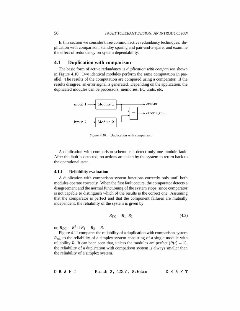
56 FAULT TOLERANT DESIGN: AN INTRODUCTION
In this section we consider three common active redundancy techniques: du-plication with comparison, standby sparing and pair-and-a-spare, and examinethe effect of redundancy on system dependability.
4.1 Duplication with comparisonThe basic form of active redundancy is duplication with comparison shown
in Figure 4.10. Two identical modules perform the same computation in par-allel. The results of the computation are compared using a comparator. If theresults disagree, an error signal is generated. Depending on the application, theduplicated modules can be processors, memories, I/O units, etc.UWVNXNY$Z][ C
UWVNXNY$Z][ G ��]���$YN� C�]���$YN� G
VHYN�;�$YN�[`beb;VHbÃi<�\�c� © ZFigure 4.10. Duplication with comparison.
A duplication with comparison scheme can detect only one module fault.After the fault is detected, no actions are taken by the system to return back tothe operational state.
4.1.1 Reliability evaluation
A duplication with comparison system functions correctly only until bothmodules operate correctly. When the first fault occurs, the comparator detects adisagreement and the normal functioning of the system stops, since comparatoris not capable to distinguish which of the results is the correct one. Assumingthat the comparator is perfect and that the component failures are mutuallyindependent, the reliability of the system is given by
RDC * R1 4 R2 (4.3)
or, RDC * R2 if R1 * R2 * R.Figure 4.11 compares the reliability of a duplication with comparison system
RDC to the reliability of a simplex system consisting of a single module withreliability R. It can been seen that, unless the modules are perfect (R % t &t* 1),the reliability of a duplication with comparison system is always smaller thanthe reliability of a simplex system.
��������� � �����������������������! �"�$# ���������

Hardware redundancy 57
B C
CJÕÔTÖ
J
J�¦ÃÂeÄ�ÅIÆ]¤
J �§ `�£¢¥¤¡¦
Figure 4.11. Duplication with comparison reliability compared to simplex system reliability.
4.2 Standby sparingStandby sparing is another scheme for active hardware redundancy. The ba-
sic configuration is shown in Figure 4.12. Only one of n modules is operationaland provides the system’s output. The remaining n 2 1 modules serve as spares.A spare is a redundant component which is not needed for the normal systemoperation. A switch is a device that monitors the active module and switchesoperation to a spare if an error is reported by fault-detection unit FD.U^V¨X�Y�Z][ C
U^V¨X�Y�Z][ GU^V¨X�Y�Z][�Ï ×Ø ÙÚ
Û]ÜÝ Ø Þßà�áà�áà�á
�]�$��YN� C�]�$��YN� G�]�$��YN�âÏ ÑÑÑ VcY��;��YN�
Figure 4.12. Standby sparing redundancy.
There are two types of standby sparing: hot standby and cold standby. Inthe hot standby sparing, both operational and spare modules are powered up.
��������� � �����������������������! �"�$# ���������

58 FAULT TOLERANT DESIGN: AN INTRODUCTION
The spares can be switched into use immediately after the operational modulehas failed. In the cold standby sparing, the spare modules are powered downuntil needed to replace the faulty module. A disadvantage of cold standbysparing is that time is needed to apply power to a module, perform initializationand re-computation. An advantage is that the stand-by spares do not consumepower. This is important in applications like satellite systems, where powerconsumption is critical. Hot standby sparing is preferable where the momentaryinterruption of normal operation due to reconfiguration need to be minimized,like in a nuclear plant control system.
A standby sparing system with n modules can tolerate n 2 1 module faults.Here by “tolerate” we mean that the system will detect and locate the faults,successfully recover from them and continue delivering the correct service.When the nth fault occurs, it will still be detected, but the system will not beable to recover back to normal operation.
Standby sparing redundancy technique is used in many systems. One exam-ple is Apollo spacecraft’s telescope mount pointing computer. In this system,two identical computers, an active and a spare, are connected to a switchingdevice that monitors the active computer and switches operation to the backupin case of a malfunction.
Another example of using standby sparing is Saturn 5 launch vehicle digitalcomputer (LVDC) memory section. The section consists of two memory blocks,with each memory being controlled by an independent buffer register and parity-checked. Initially, only one buffer register output is used. When a parity erroris detected in the memory being used, operation immediately transfers to theother memory. Both memories are then re-generated by the buffer register ofthe "correct" memory, thus correcting possible transient faults.
Standby sparing is also used in Compaq’s NonStop Himalaya server. Thesystem is composed of a cluster of processors working in parallel. Each proces-sor has its own memory and copy of the operating system. A primary processand a backup process are run on separate processors. The backup process mir-rors all the information in the primary process and is able to instantly take overin case of a primary processor failure.
4.2.1 Reliability evaluation
By their nature, standby systems involve dependency between components,since the spare units are held in reserve and only brought to operation in theevent the primary unit fails. Therefore, standby systems are best analyzedusing Markov models. We first consider an idealized case when the switchingmechanism is perfect. We also assume that the spare cannot fail while it is in thestandby mode. Later, we consider the possibility of failure during switching.
Perfect switching case
��������� � �����������������������! �"�$# ���������

Hardware redundancy 59UWVNXNY$Z][ CUWVNXNY$Z][ G ã Ø ÙÚÛ]ÜÝ
Ø Þßà�áà�á
�]���$YN� C�]���$YN� G VcYN�e��YN�
Figure 4.13. Standby sparing system with one spare.
Consider a standby sparing scheme with one spare, shown in Figure 4.13.Let module 1 be a primary module and module 2 be a spare. The state transi-tion diagram of the system is shown in Figure 4.14. The states are numberedaccording to the Table 4.2.
Component State1 2 NumberO O 1F O 2F F 3
Table 4.2. Markov states of the state transition diagram of a standby sparing system with onespare.
When the primary component fails, there is a transition between the state 1and state 2. If a system is in the state 2 and the spare fails, there is a transitionto the state 3. Since we assumed that the spare cannot fail while in the standbymode, the combination % O ( F & cannot occur. The states 1 and 2 are operationalstates. The state 3 is the failed state.C G D>po >7q
Figure 4.14. State transition diagram of a standby sparing system with one spare.
The transition matrix for the state transition diagram 4.14 is given by
M * |� 2 λ1 0 0λ1 2 λ2 00 λ2 0
�� -��������� � �����������������������! �"�$# ���������

60 FAULT TOLERANT DESIGN: AN INTRODUCTION
So, we get the following system of state transition equations
ddt |� P1 % t &
P2 % t &P3 % t &
�� * |� 2 λ1 0 0λ1 2 λ2 00 λ2 0
�� 4 |� P1 % t &P2 % t &P3 % t &
��or ���� ��� d
dt P1 % t &T*�2 λ1P1 % t &ddt P2 % t &T* λ1P1 % t &�2 λ2P2 % t &ddt P3 % t &T* λ2P2 % t &
By solving the system of equations, we get
P1 % t &�* e A λ1t
P2 % t &�* λ1λ2 A λ1
% e A λ1t 2 e A λ2t &P3 % t &�* 1 2 1
λ2 A λ1% λ2e A λ1t 2 λ1e A λ2t &
Since P3 % t & is the only state corresponding to system failure, the reliability ofthe system is the sum of P1 % t & and P2 % t &
RSS % t &T* e A λ1t 5 λ1
λ2 2 λ1% e A λ1t 2 e A λ2t &
This can be re-written as
RSS % t &T* e A λ1t 5 λ1
λ2 2 λ1e A λ1t % 1 2 e A . λ2 A λ1 � t & (4.4)
Assuming % λ2 2 λ1 & t ³ä³ 1, we can expand the term e A . λ2 A λ1 � t as a power seriesof 2´% λ2 2 λ1 & t as
e A . λ2 A λ1 � t * 1 2u% λ2 2 λ1 & t 5 1 8 2 % λ2 2 λ1 & 2t2 2v-R-R-Substituting it in (4.4), we get
RSS % t &T* e A λ1t 5 λ1e A λ1t % t 2 1 8 2 % λ1 2 λ2 & t2 5å-R-R-]&!-Assuming λ2 * λ1, the above can be simplified to
RSS % t &T*æ% 1 5 λt & e A λt (4.5)
Next, let us see how the equation (4.5) would change if we would ignore thedependency between the failures. If the primary and spare modules failures aretreated as mutually independent, the reliability of a standby sparing system is a
��������� � �����������������������! �"�$# ���������
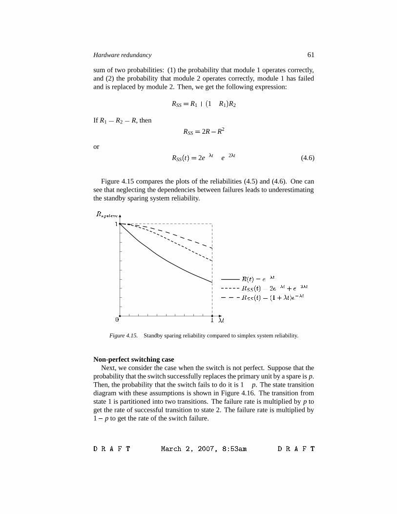
Hardware redundancy 61
sum of two probabilities: (1) the probability that module 1 operates correctly,and (2) the probability that module 2 operates correctly, module 1 has failedand is replaced by module 2. Then, we get the following expression:
RSS * R1 5% 1 2 R1 & R2
If R1 * R2 * R, then
RSS * 2R 2 R2
or
RSS % t &�* 2e A λt 2 e A 2λt (4.6)
Figure 4.15 compares the plots of the reliabilities (4.5) and (4.6). One cansee that neglecting the dependencies between failures leads to underestimatingthe standby sparing system reliability.
B C
C
JÐçFç ? =<@ � G»èHépê ¢ ë ècé q ê ¢JÐçFç ? =<@ � ? C ë > =;@ èHépê ¢J ? =<@ � è épê ¢> =
JÐ�§ `�£¢¥¤¡¦
Figure 4.15. Standby sparing reliability compared to simplex system reliability.
Non-perfect switching caseNext, we consider the case when the switch is not perfect. Suppose that the
probability that the switch successfully replaces the primary unit by a spare is p.Then, the probability that the switch fails to do it is 1 2 p. The state transitiondiagram with these assumptions is shown in Figure 4.16. The transition fromstate 1 is partitioned into two transitions. The failure rate is multiplied by p toget the rate of successful transition to state 2. The failure rate is multiplied by1 2 p to get the rate of the switch failure.
��������� � �����������������������! �"�$# ���������

62 FAULT TOLERANT DESIGN: AN INTRODUCTION
C G Dì >po ? C¶m ì @ > o >7qFigure 4.16. State transition diagram of a standby system with one spare.
The state transition equations corresponding to the state transition diagram(4.16) are ���� ��� d
dt P1 % t &T*�2 λ1P1 % t &ddt P2 % t &T* pλ1P1 % t &�2 λ2P2 % t &ddt P3 % t &T* λ2P2 % t &65% 1 2 p & λ1P1 % t &
By solving this system of equations, we get
P1 % t &�* e A λ1t
P2 % t &�* pλ1λ2 A λ1
% e A λ1t 2 e A λ2t &P3 % t &�* 1 2u% 1 5 pλ1
λ2 A λ1& e A λ1t 5 pλ1
λ2 A λ1e A λ2t
As before, P3 % t & corresponds to system failure. So, the reliability of the systemis the sum of P1 % t & and P2 % t &
RSS % t &T* e A λ1t 5 pλ1
λ2 2 λ1% e A λ1t 2 e A λ2t &
Assuming λ2 * λ1, the above can be simplified to
RSS % t &T*�% 1 5 pλt & e A λt (4.7)
Figure 4.17 compares the reliability of a standby sparing system for differentvalues of p. As p decreases, the reliability of the standby sparing systemdecreases. When p reaches zero, the standby sparing system reliability reducesto the reliability of a simplex system.
4.3 Pair-and-a-sparePair-and-a-spare technique combines standby sparing and duplication and
comparison approaches (Figure 4.18). The idea is similar to standby sparing,however two modules instead of one are operated in parallel. As in duplicationwith comparison case, the results are compared to detect disagreement. If anerror signal is received from the comparator, the switch analyzes the report
��������� � �����������������������! �"�$# ���������
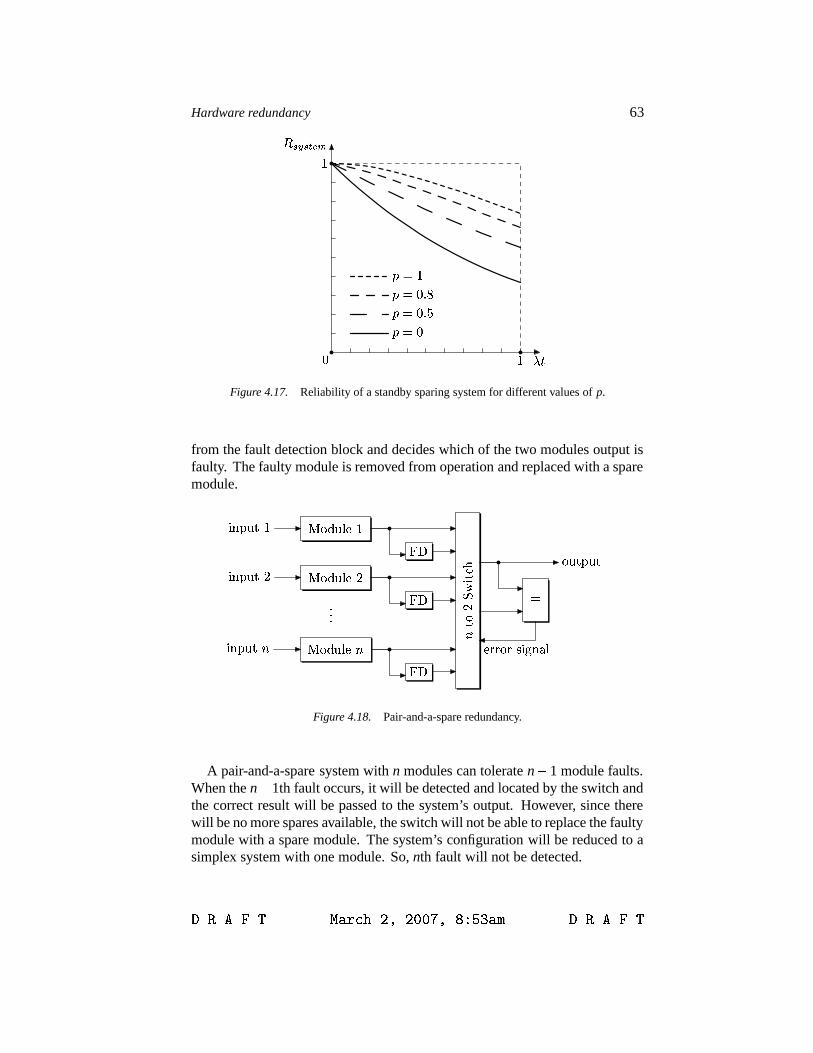
Hardware redundancy 63
B C
Cì � Cì � B�í îì � B�í ½ì � B > =
J��¡ `�£¢¥¤§¦
Figure 4.17. Reliability of a standby sparing system for different values of p.
from the fault detection block and decides which of the two modules output isfaulty. The faulty module is removed from operation and replaced with a sparemodule. UWVNXNY$Z][ C
UWVNXNY$Z][ GUWVNXNY$Z][�Ï ×Ø Ù
ãÛ]ÜÝ Ø Þßà�áà�áà�á
��]���$YN� C�]���$YN� G�]���$YN�âÏ ÑÑÑ [`beb;VHbÃi;�]�H� © Z
VHYN�;�$YN�
Figure 4.18. Pair-and-a-spare redundancy.
A pair-and-a-spare system with n modules can tolerate n 2 1 module faults.When the n 2 1th fault occurs, it will be detected and located by the switch andthe correct result will be passed to the system’s output. However, since therewill be no more spares available, the switch will not be able to replace the faultymodule with a spare module. The system’s configuration will be reduced to asimplex system with one module. So, nth fault will not be detected.
��������� � �����������������������! �"�$# ���������

64 FAULT TOLERANT DESIGN: AN INTRODUCTION
5. Hybrid redundancyThe main idea of hybrid redundancy is to combine the attractive features
of passive and active approach. Fault masking is used to prevent system fromproducing momentary erroneous results. Fault detection, location and recoveryare used to reconfigure the system after a fault occurs. In this section, we con-sider three basic techniques for hybrid redundancy: self-purging redundancy,N-modular redundancy with spares and triplex-duplex redundancy.
5.1 Self-purging redundancySelf-purging redundancy consists of n identical modules which are actively
participating in voting (Figure 4.19). The output of the voter is compared tothe outputs of individual modules to detect disagreement. If a disagreementoccurs, the switch opens and removes, or purges, the faulty module from thesystem. The voter is designed as a threshold gate, capable to adapt to thechanging number of inputs. The input of the removed module is forced to zeroand therefore do not contribute to the voting.
º+V»�e[`bUWVNXNY�Z\[ CUWVNXNY�Z\[ GUWVNXNY�Z\[�Ï
ï Cï Gï Ï
�\����YN� C�\����YN� G�\����YN� D
VcYN�e��YN�ÑÑÑFigure 4.19. Self-purging redundancy.
A self-purging redundancy system with n modules can mask n 2 2 modulefaults. When n 2 2 modules are purged and only two are left, the system will beable to detect next, n 2 1th fault, but, as in duplication with comparison case,voter will not be able to distinguish which of the results is the correct one.
5.1.1 Reliability evaluation
Since all modules of the system operate in parallel, we can assume thatthe modules failures are mutually independent. It is sufficient that two of themodules of the system function correctly for the system to be operational. Ifthe voter and the switches are perfect, and if all the modules have the samereliability R1 * R2 *ð-R-R-6* Rn * R, then the system is not reliable if all the
��������� � �����������������������! �"�$# ���������

Hardware redundancy 65
modules have failed (probability % 1 2 R & n), or if all but one modules have failed(probability R % 1 2 R & n A 1). Since there are n choices for one of n modules toremain operational, we get the equation
RSP * 1 2u%R% 1 2 R & n 5 nR % 1 2 R & n A 1 & (4.8)
Figure 4.20 compares the reliabilities of self-purging redundancy systemswith three, five and seven modules.
B C
CC _�VNXNY$Z][D _�VNXNY$Z][Ii½ _�VNXNY$Z][IiÇ _�VNXNY$Z][Ii J�¦ÃÂeÄ�ÅIÆ]¤
JÐ�§ `�£¢¥¤¡¦
Figure 4.20. Reliability of a self-purging redundancy system with 3, 5 and 7 modules.
5.2 N-modular redundancy with sparesN-modular redundancy with k spares is similar to self-purging redundancy
with k 5 n modules, except that only n modules provide input to a majorityvoter (Figure 4.21). Additional k modules serve as spares. If one of the primarymodules become faulty, the voter will mask the erroneous result and the switchwill replace the faulty module with a spare one. Various techniques are usedto identify faulty modules. One approach is to compare the output of the voterwith the individual outputs of the modules, as shown in Figure 4.21. A modulewhich disagrees with the majority is declared faulty.
The fault-tolerant capabilities of an N-modular redundancy system with kspares depend on the form of voting used as well as the implementation of theswitch and comparator. One possibility is that, after the spares are exhausted,the disagreement detector is switched off and the system continues workingas a passive NMR system. Then, such a system can mask
Ín 8 2 Îâ5 k faults,
i.e. the number of faults a NMR system can mask plus the number of spares.
��������� � �����������������������! �"�$# ���������

66 FAULT TOLERANT DESIGN: AN INTRODUCTION
×Ù ñØ Ùò ×óôÛ]ÜÝ Ø Þß
UWVNXNY�Z\[ CUWVNXNY�Z\[ GUWVNXNY�Z\[�Ïï � © be[ Cï � © b;[öõ
º+Vc�;[!b
��\����Y�� C�\����Y�� G�\����Y��âÏ VcY��;��YN�ÑÑÑ
ÑÑÑÑÑÑ
í`í`í í!í`í
Figure 4.21. N-modular redundancy with spares.
Another possibility is that the disagreement detector remains on, but the voter isdesigned to be capable to adjust to the decreasing number of inputs. In this case,the behavior of the system is similar to the behavior of a self-purging systemwith n 5 k modules, i.e. up to k 5 n 2 2 module faults can be masked. Supposethe spares are exhausted after the first k faults, and the k 5 1th fault occurred.As before, the erroneous result will be masked by the voter, the output of thevoter will be compared to the individual outputs of the modules, and the faultywill be removed from considerations. A difference is that it will not be replacedwith a spare one, but instead the system will continue working as n 2 1-modularsystem. Then a k 5 ith fault occurs, the voter votes on n 2 i & modules.
5.3 Triplex-duplex redundancyTriplex-duplex redundancy combines triple modular redundancy and dupli-
cation with comparison (Figure 4.22). A total of six identical modules, groupedin three pairs, are computing in parallel. In each pair, the results of the com-putation are compared using a comparator. If the results agree, the output ofthe comparator participate in the voting. Otherwise, the pair of modules isdeclared faulty and the switch removes the pair from the system. In this way,only faulty-free pair participate in voting.
��������� � �����������������������! �"�$# ���������

Hardware redundancy 67UWVNXNY�Z\[ C ©UWVNXNY�Z\[ C ª � ï CUWVNXNY�Z\[ G ©UWVNXNY�Z\[ G ª � ï GUWVNXNY�Z\[ D ©UWVNXNY�Z\[ D ª � ï D
º+Vc�;[`b�\����YN� C ©�]�$��YN� C ª�\����YN� G ©�]�$��YN� G ª�\����YN� D ©�]�$��YN� D ª
VHYN�;��Y��
Figure 4.22. Triplex-duplex redundancy.
6. Problems4.1. Explain the difference between passive, active and hybrid hardware redun-
dancy. Discuss the advantages and disadvantages of each approach.
4.2. Suppose that in the system shown in Figure 4.1 the two components havethe same cost and R1 * 0 - 75, R2 * 0 - 96. If it is permissible to add twocomponents to the system, would it be preferable to replace component 1 bya three-component parallel system, or to replace components 1 and 2 eachby two-component parallel systems?
4.3. A disk drive has a constant failure rate and an MTTF of 5500 hr.
(a) What is the probability of failure for one year of operation?
(b) What is the probability of failure for one year of operation if two of thedrives are placed in parallel and the failures are independent?
4.4. Construct the Markov model of the TMR system with three voters shown inFigure 4.6. Assume that the components are independent. The failure rateof the modules is λm. The failure rates of the voters is λv. Derive and solvethe system of state transition equations representing this system. Computethe reliability of the system.
4.5. Draw a logic diagram of a majority voter with 5 inputs.
4.6. Suppose the design life reliability of a standby system consisting of twoidentical units should be at least 0.97. If the MTTF of each unit is 6 months,
��������� � �����������������������! �"�$# ���������

68 FAULT TOLERANT DESIGN: AN INTRODUCTION
determine the design life time. Assume that the failures are independentand ignore switching failures.
4.7. An engineer designs a system consisting of two subsystems in series withthe reliabilities R1 * 0 - 99 and R2 * 0 - 85. The cost of the two subsystemsis approximately the same. The engineer decides to add two redundantcomponents. Which of the following is the best to do:
(a) Duplicate subsystems 1 and 2 in high-level redundancy (Figure 4.2(a)).
(b) Duplicate subsystems 1 and 2 in low-level redundancy (Figure 4.2(b)).
(c) Replace the second subsystem by a three-component parallel system.
4.8. A computer with MTTF of 3000 hr is to operate continuously on a 500 hrmission.
(a) Compute computer’s mission reliability.
(b) Suppose two such computers are connected in a standby configuration.If there are no switching failures and no failures of the backup computerwhile in the standby mode, what is the system MTTF and the missionreliability?
(c) What is the mission reliability if the probability of switching failure is0.02?
4.9. A chemical process control system has a reliability of 0.97. Because reli-ability is considered too low, a redundant system of the same design is tobe installed. The design engineer should choose between a parallel and astandby configuration. How small must the probability of switching failurebe for the standby configuration to be more reliable than the parallel con-figuration? Assume that there is no failures of the backup system while inthe standby mode.
4.10. Give examples of applications where you would recommend to use coldstandby sparing and hot standby sparing (two examples each). Justify youranswer.
4.11. Compare the MTTF of a standby spare system with 3 modules and a pair-and-a-spare system with 3 modules, provided the failure rate of a singlemodule is 0.01 failures per hour. Assume the modules obey the exponentialfailure law. Ignore the switching failures and the dependency between themodule’s failures.
4.12. A basic non-redundant controller for a heart pacemaker consists of an analogto digital (A/D) converter, a microprocessor and a digital to analog (D/A)converter. Develop a design making the controller tolerant to any two com-ponent faults (component here means A/D converter, microprocessor or D/A
��������� � �����������������������! �"�$# ���������

Hardware redundancy 69
converter). Show the block diagram of your design and explain why yourecommend it.
4.13. Construct the Markov model of a hybrid N-modular redundancy with 3 activemodules and one spare. Assume that the components are independent andthat the probability that the switch successfully replace the failed moduleby a spare is p.
4.14. How many faulty modules can you tolerate in:
(a) 5-modular passive redundancy?
(b) standby sparing redundancy with 5 modules?
(c) self-purging hybrid modular redundancy with 5 modules?
4.15. Design a switch for hybrid N-modular redundancy with 3 active modulesand 1 spare.
4.16. (a) Draw a diagram of standby sparing active hardware redundancy tech-nique with 2 spares.
(b) Using Markov models, write an expression for the reliability of systemyou showed on the diagram for
(a) perfect switching case,(b) non-perfect switching case.(c) Calculate the reliabilities for (a) and (b) after 1000 hrs for the failure
rate λ * 0 - 01 per 100 hours.
4.17. Which redundancy would you recommend to combine with self-purginghybrid hardware redundancy to distinguish between transient and perma-nent faults? Briefly describe what would be the main benefit of such acombination.
4.18. Calculate the MTTF of a 5-modular hardware redundancy system, pro-vided the failure rate of a single module is 0.001 failures per hour. Assumethe modules obey the exponential failure law. Compare the MTTF of the5-modular redundancy system with the MTTF of a 3-modular hardwareredundancy system having the failure rate 0.01 failures per hour.
4.19. Draw simplified Markov model for 5-modular hardware redundancy schemewith failure rate λ. Explain which state of the system each of the nodes inyour chain represents.
��������� � �����������������������! �"�$# ���������


Chapter 5
INFORMATION REDUNDANCY
The major difference between a thing that might go wrong and a thing that cannot possiblygo wrong is that when a thing that cannot possibly go wrong goes wrong it usually turnsout to be impossible to get at or repair.
—Douglas Adams, "Mostly Harmless"
1. IntroductionIn this chapter we study how fault-tolerance can be achieved by means of
encoding. Encoding is the powerful technique allowing us to ensure that infor-mation has not been changed during storage or transmission. Attaching specialcheck bits to blocks of digital information enables special-purpose hardwareto detect and correct a number of communication and storage faults, such aschanges in single bits or changes to several adjacent bits. Parity code usedfor memories in computer systems is a common example of an application ofencoding. Another example is communication protocols, providing a varietyof detection and correction options, including the encoding of large blocks ofdata to withstand multiple faults and provisions for multiple retries in case errorcorrecting facilities cannot cope with faults.
Coding theory was originated in the late 1940s, by two seminal works byHamming and Shannon. Hamming, working at Bell Laboratories in the USA,was studying possibilities for protecting storage devices from the corruption ofa small number of bits by a code which would be more efficient than simplerepetition. He realized the need to consider sets of words, or codewords, whereevery pair differs in a large number of bit positions. Hamming defined the notionof distance between two words and observed this was a metric, thus leading tointeresting properties. This distance is now called Hamming distance. His firstattempt produced a code in which four data bits were followed by three check
��������� � �����������������������! �"�$# ���������

72 FAULT TOLERANT DESIGN: AN INTRODUCTION
bits which allowed not only the detection but the correction of a single error.The repetition code would require nine check bits to achieve this. Hammingpublished his results in 1950.
Slightly prior to Hamming’s publication, in 1948, Shannon, also at Bell Labs,wrote an article formulating the mathematics behind the theory of communi-cation. In this article, he developed probability and statistics to formalize thenotion of information. Then, he applied this notion to study how a sender cancommunicate efficiently over different media, or more generally, channels ofcommunication to a receiver. The channels under consideration were of twodifferent types: noiseless or noisy. In the former case, the goal is to compressthe information at the sender’s end and to minimize the total number of symbolscommunicated while allowing the receiver to recover transmitted informationcorrectly. The later case, which is more important to the topic of this book,considers a channel that alters the signal being sent by adding to it a noise. Thegoal in this case is to add some redundancy to the message being sent so that afew erroneous symbols at the receiver’s end still allow the receiver to recover thesender’s intended message. Shannon’s work showed, somewhat surprisingly,that same underlying notions captured the rate at which one could communicateover either class of channels. Shannon’s methods involved encoding messagesusing long random strings, and the theory relied on the fact that long messageschosen at random tend to be far away from each other. Shannon had shown thatit was possible to encode messages in such a way that the number of extra bitstransmitted was as small as possible.
Although Shannon’s and Hamming’s works were chronologically and tech-nically interwined, both researchers seem to regard the other as far away fromtheir own work. Shannon’s papers never explicitly refers to distance in his maintechnical results. Hamming, in turn, does not mention the applicability of hisresults to reliable computing. Both works, however, were immediately seento be of monumental impact. Shannon’s results started driving the theory ofcommunication and storage of information. This, in turn, became the primarymotivation for much research in the theory of error-correcting codes.
The value of error-correcting codes for transmitting information becameimmediately apparent. A wide variety of codes were constructed, achievingboth economy of transmission and error-correction capacity. Between 1969and 1973 the NASA Mariner probes used a powerful Reed-Muller code capableof correcting 7 errors out of 32 bits transmitted. The codewords consisted of 6data bits and 26 check bits. The data was sent to Earth on the rate over 16,000bits per second.
Another application of error-correcting codes came with the development ofthe compact disk (CD). To guard against scratches, cracks and similar damagetwo "interleaved" codes which can correct up to 4,000 consecutive errors (about2.5 mm of track) are used.
��������� � �����������������������! �"�$# ���������

Information redundancy 73
Code selection is usually guided by types of errors required to be toleratedand the overhead associated with each of the error detection techniques. Forexample, error correction is a common level of protection for minicomputersand mainframes whereas the cheaper error detection by parity code is morecommon in microcomputers. For solid state disks, storing system’s critical,non-recoverable files, the most popular codes are Hamming codes to correcterrors in main memory, and Reed-Solomon codes to correct errors in peripheraldevices such as tape and disk storage.
2. Fundamental notions
In this section, we introduce the basic notions of coding theory. We assumethat our data is in the form of strings of binary bits, 0 or 1. We also assumethat the errors occur randomly and independently from each other, but at apredictable overall rate.
2.1 Code
A binary code of length n is a set of binary n-tuples satisfying some well-defined set of rules. For example, an even parity code contains all n-tuplesthat have an even number of 1s. The set Bn *�P 0 ( 1 S n of all possible 2n binaryn-tuples is called codespace.
A codeword is an element of the codespace satisfying the rules of the code.To make error-detection and error-correction possible, codewords are chosento be a nonempty subset of all possible 2n binary n-tuples. For example, aparity code of length n has 2n A 1 codewords, which is one half of all possible 2n
n-tuples. An n-tuple not satisfying the rules of the code is called a word.
The number of codewords in a code C is called the size of C, denoted by 3C 3 .2.2 Encoding
Encoding is the process of computing a codeword for a given data. Anencoder takes a binary k-tuple representing the data and converts it to a codewordusing the rules of the code. For example, to compute a codeword for an evenparity code, the parity of the data is first determined. If the parity is odd, a1-bit is attached to the end of the k-tuple. Otherwise, a 0-bit is attached. Thedifference n 2 k between the length n of the codeword and the length k of thedata gives the number of check bits which must be added to the data to do theencoding. Separable code is a code in which check bits can be clearly separatedfrom data bits. Parity code is an example of a separable code. Non-separablecode is a code in which check bits cannot be separated from data bits. Cycliccode is an example of a non-separable code.
��������� � �����������������������! �"�$# ���������
74 FAULT TOLERANT DESIGN: AN INTRODUCTION
2.3 Information rateTo encode binary k-bit data, we need a code consisting of at least 2k code-
words, since any data word should be assigned its own individual codewordfrom C. Vice versa, a code of size 3C 3 encodes the data of length k 0æ÷ log2 3C 3 øbits. The ratio k 8 n is called the information rate of the code. The informationrate determines the redundancy of the code. For example, a repetition codeobtained by repeating the data three times, has the information rate 1 8 3. Onlyone out of three bits carries the message, two others are redundant.
2.4 DecodingDecoding is the process of restoring data encoded in a given codeword. A
decoder reads a codeword and recovers the original data using the rules of thecode. For example, decoder for a parity code truncates the codeword by onebit.
Suppose that an error has occurred and a non-codeword is received by adecoder. A usual assumption in coding theory is that a pattern of errors thatinvolves a small number of bits is more likely to occur than any pattern thatinvolves a large number of bits. Therefore, to perform decoding, we search fora codeword which is “closest” to the received word. Such a technique is calledmaximum likelihood decoding. As a measure of distance between two binaryn-tuples x and y we use Hamming distance.
2.5 Hamming distanceHamming distance between two binary n-tuples, x and y, denoted by δ % x ( y & ,
is the number of bit positions in which the n-tuples differ. For example, x * 0011and y * 0101 differ in 2 bit positions, so δ % x ( y &1* 2. Hamming distance givesus an estimate of how many bit errors have to occur to change x into y.
Hamming distance is a genuine metric on the codespace Bn. A metric isa function that associates any two objects in a set with a number and thatpreserves a number of properties of the distance with which we are familiar.These properties are formulated in the following three axioms:
1 δ % x ( y &�* 0 if and only if x * y.
2 δ % x ( y &�* δ % y ( x & .3 δ % x ( y &65 δ % y ( z &úù δ % x ( z & .
Metric properties of Hamming distance allow us to use the geometry of thecodespace to reason about the codes. As an example, consider the codespaceB3 presented by a three-dimensional cube shown in Figure 5.1. CodewordsP 000 ( 011 ( 101 ( 110 S are marked with large solid dots. Adjacent vertices differby a single bit. It is easy to see that Hamming distance satisfies the metric
��������� � �����������������������! �"�$# ���������

Information redundancy 75
B�CIBCIBcB
BHB�CCcCcC
BcBHB
B$CcCC!B�CCHC!B
Figure 5.1. Code û 000 ü 011 ü 101 ü 110 ý in the codespace B3.
properties of Hamming distance listed above, e.g. δ % 000 ( 011 &$5 δ % 011 ( 111 &Ã*2 5 1 * 3 * δ % 000 ( 111 & .2.6 Code distance
Code distance of a code C is the minimum Hamming distance between anytwo distinct pairs of codewords of C. For example, code distance of a paritycode equals two. Code distance determines the error detecting and correctingcapabilities of a code. For instance, consider the code P 000 ( 011 ( 101 ( 110 S inFigure 5.1. The code distance of this code is two. Any one-bit error in anycodeword produces a word laying on distance one from the affected codeword.Since all codewords are on distance two from each other, the error will bedetected.
As another example, consider the code P 000 ( 111 S shown in Figure 5.2. The
B�CIBCIBcB
BHB�CCcCcC
BcBHB
B$CcCC!B�CCHC!B
Figure 5.2. Code û 000 ü 111 ý in the codespace B3.
codewords are marked with large solid dots. Suppose an error occurred in thefirst bit of the codeword 000. The resulting word 100 is on distance one from000 and on distance two from 111. Thus, we correct 100 to the codeword 000,which is closest to 100 according to the Hamming distance.
��������� � �����������������������! �"�$# ���������

76 FAULT TOLERANT DESIGN: AN INTRODUCTION
The code P 000 ( 111 S is a replication code, obtained by repeating the data threetimes. One one bit of a codeword carries the data, two others are redundant.By its nature, this redundancy is similar to TMR, but it is implemented in theinformation domain. In TMR, voter compares the output values of the modules.In a replication code, a decoder analyzes the bits of the received word. In bothcases, majority of values of bits determines the decision.
In general, to be able to correct ε-bit errors, a code should have the codedistance of at least 2ε 5 1. To be able to detect ε-bit errors, the code distanceshould be at least ε 5 1.
2.7 Code efficiencyThroughout the chapter, we evaluate the efficiency of a code using the fol-
lowing three criteria:
1 Number bit errors a code can detect/correct, reflecting the fault tolerantcapabilities of the code.
2 Information rate k 8 n, reflecting the amount of information redundancy added.
3 Complexity of encoding and decoding schemes, reflecting the amount ofhardware, software and time redundancy added.
The first item in the list above is the most important. Ideally, we would liketo have a code that is capable of correcting all errors. The second objective isan efficiency issue. We would rather not waste resources by exchanging dataon a very low rate. Easy encoding and decoding schemes are likely to have asimple implementation in either hardware or software. They are also desirablefor efficiency reasons. In general, the more errors that a code needs to correctper message digit, the less efficient the communication and usually the morecomplicated the encoding and decoding schemes. A good code balances theseobjectives.
3. Parity codesParity codes are the oldest family of codes. They have been used to detect
errors in the calculations of the relay-based computers of late 1940’s.The even (odd) parity code of length n is composed of all binary n-tuples that
contain an even (odd) number of 1’s. Any subset of n 2 1 bits of a codewordcan be viewed as data bits, carrying the information, while the remaining nth bitchecks the parity of the codeword. Any single-bit error can be detected, sincethe parity of the affected n-tuple will be odd (even) rather than even (odd). It isnot possible to locate the position of the erroneous bit. Thus, it is not possibleto correct it.
��������� � �����������������������! �"�$# ���������

Information redundancy 77
The most common application of parity is error-detection in memories ofcomputer systems. A diagram of a memory protected by a parity code is shownin Figure 5.3.
UW[`_aVHb;dftþf1ÿ� �Ø �� ñ�
[`beb;VHbÃi;�]�H� © Z� �Ø �� ñ�
á © � © :§�á © � ©�� Y��f © b;�]�§df © be�]�§d
Figure 5.3. A memory protected by a parity code; PG = parity generator; PC = parity checker.
Before being written into a memory, the data is encoded by computing itsparity. In most computer systems, one parity bit per byte (8 bits) of data iscomputed. The generation of parity bits is done by a parity generator (PG)implemented as a tree of exclusive-OR (XOR) gates. Figure 5.4 shows a logicdiagram of an even parity generator for 4-bit data % d0 ( d1 ( d2 ( d3 & .É É É
����No�Fq� Ë � © b;�]�§d ª � �
Figure 5.4. Logic diagram of a parity generator for 4-bit data K d0 ü d1 ü d2 ü d3 L .When data is written into memory, parity bits are written along with the
corresponding bytes of data. For example, for a 32-bit word size, four paritybits are attached to data and a 36-bit codeword is stored in the memory. Somesystems, like Pentium processor, have a 64-bit wide memory data path. In thesecase, eight parity bits are attached to data. The resulting codeword 72 bit long.
When the data is read back from the memory, parity bits are re-computedand the result is compared to the previously stored parity bits. Re-computationof parity is done by a parity checker (PC). Figure 5.5 shows a logic diagramof an even parity checker for 4-bit data % d0 ( d1 ( d2 ( d3 & . The logic diagram issimilar to the one of a parity generator, except that one more XOR gate is added
��������� � �����������������������! �"�$# ���������

78 FAULT TOLERANT DESIGN: AN INTRODUCTION
to compare the re-computed parity bit to the previously stored parity bit. If theparity bits disagree, the output of the XOR gate is 1. Otherwise, the output is0. É É É É
� ��No�Fq� Ë� © be� �§d ª �]� [`beb;VHb1� C
Figure 5.5. Logic diagram of a parity checker for 4-bit data K d0 ü d1 ü d2 ü d3 L .Any computed parity bit that does not match the stored parity bit indicates
that there was at least one bit error in the corresponding byte of data, or in theparity bit itself. An error signal, called non-maskable interrupt, is sent to theCPU to indicate that the memory data is not valid and to instruct the processorto immediately halt.
All operations related to the error-detection (encoding, decoding, compari-son) are done by memory control logic on the mother-board, in the chip set, or,for some systems, in the CPU. The memory itself only stores the parity bits,just as it stores the data bits. Therefore, parity checking does not slow downthe operation of the memory. The parity bit generation and checking is donein parallel with the writing and reading of the memory using the logic whichis much faster that the memory itself. Nothing in the system waits for a “noerror” signal from the parity checker. The system only performs an action ofinterrupt when it finds an error.
Example 5.1. Suppose the data which is written in the memory is [0110110]and odd-parity code is used. Then the check bit 1 is stored along with the data,to make the overall parity odd. Suppose that the data read out of the memoryis [01111100]. The re-computed parity is 0. Because the re-computed paritydisagree with the stored parity, we know that an error has occurred.
Parity can only detect single bit errors and an odd number of bit errors. If aneven number of bits are affected, the computed parity matches the stored parity,and the erroneous data is accepted with no error notification, possibly causinglater some mysterious problems. Studies have shown that approximately 98%of all memory errors are single-bit errors. Thus, protecting a memory by aparity code is an inexpensive and efficient technique. For example, 1 GBytedynamic random access (DRAM) memory with a parity code has a failure rate
��������� � �����������������������! �"�$# ���������

Information redundancy 79
of 0.7 failures per year. If the same memory uses a single-error correctiondouble-error detection Hamming code, requiring 7 check bits in a 32-bit widememory system, then the failure rate reduces to 0.03 failures per year. An errorcorrecting memory is typically slower than a non-correcting one, due to theerror correcting circuitry. Depending on the application, 0.7 failures per yearmay be viewed as an acceptable level of risk, or not.
A modification of parity code is horizontal and vertical parity code, whicharrange the data in a 2-dimensional array and add one parity bit on each rowand one parity bit on each column. Such a technique is useful for correctingsingle bit errors within a block of data words, however, it may fail correctingmultiple errors.
4. Linear codesLinear codes provide a general framework for generating many codes, includ-
ing Hamming code. The discussion of linear codes requires some knowledgeof linear algebra, which we first briefly review.
4.1 Basic notionsField Z2. A field Z2 is the set P 0 ( 1 S together with two operations, addition“ 5 ” and multiplication “ 4 ”, such that the following properties are satisfied forall a ( b ( c � Z2:
1 Z2 is closed under ‘ 4 ” and “ 5 ”, meaning that a 4 b � Z2 and a 5 b � Z2.
2 a 5% b 5 c &+*�% a 5 b &65 c.
3 a 5 b * b 5 a
4 There exists an element 0 in Z2 such that a 5 0 * a.
5 For each a � Z2, there exists an element 2 a � Z2 such that a 5%�2 a &+* 0.
6 a 4·% b 4 c &�*�% a 4 b & 4 c.
7 a 4 b * b 4 a.
8 There exists an element 1 in Z2 such that a 4 1 * 1 4 a * a.
9 For each a � Z2, such that a y* 0, there exists an element a A 1 � Z2 such thata 4 a A 1 * 1.
10 a 4·% b 5 c &�* a 4 b 5 a 4 c.
It is easy to see that above properties are satisfied if “ 5 ” is defined as additionmodulo 2, “ 4 ” is defined as multiplication modulo 2, 0 = 0 and 1 = 1. Throughoutthe chapter, we assume this definition of Z2.
��������� � �����������������������! �"�$# ���������

80 FAULT TOLERANT DESIGN: AN INTRODUCTION
Vector space V n. Let Zn2 denote the set of all n-tuples containing elements
from Z2. For example, for n * 3, Z32 *�P 000 ( 001 ( 010 ( 011 ( 100 ( 110 ( 111 S .
A vector spaceV n over a field Z2 is subset of Zn2 , with two operations, addition
“ 5 ” and multiplication “ 4 ”, such that the following axioms are satisfied for allx ( y ( z � V n and all a ( b ( c � Zn:
1 V n is closed under “ 5 ”, meaning that x 5 y � V n.
2 x 5 y * y 5 x.
3 x 5% y 5 z &+*�% x 5 y &65 z.
4 There exists an element 0 in V n such that x 5 0 * x.
5 For each x � V n, there exists an element 2 x � V n such that x 5%�2 x &+* 0.
6 a 4 x � V n.
7 There exists an element 1 � Z2 such that 1 4 x * x.
8 a 4·% x 5 y &T*�% a 4 x &65�% a 4 y & .9 % a 5 b &�4 x * a 4 x 5 b 4 x.
10 % a 4 b &�4 x * a 4 % b 4 x & .A subspace is a subset of a vector space that is itself a vector space.A set of vectors P v0 (R-R-R-`( vk A 1 S is said to span a vector space V n if any v � V n
can be written as v * a0v0 5 a1v1 5å-R-R-R5 ak A 1vk A 1, where a0 (R-R-R-h( ak A 1 � Z2.A set of vectors P v0 (R-R-R-h( vk A 1 S of V n is said to be linearly independent if
a0v0 5 a1v1 5¸-R-R-�5 ak A 1vk A 1 * 0 implies that a0 * a1 * -R-R-H* ak A 1 * 0. If a setof vectors is not linearly independent then they are linearly dependent.
A basis is a set of vectors in a vector space V n that are linearly independentand span V n.
The dimension of a vector space is defined to be the number of vectors in itsbasis.
4.2 Definition of linear codeA % n ( k & linear code over the field Z2 is a k-dimensional subspace of Vn. In
other words, a linear code of length n is a subspace of V n which is spannedby k linearly independent vectors. All codewords can be written as a linearcombination of the k basis vectors P v0 (R-R-R-h( vk A 1 S as follows:
c * d0v0 5 d1v1 5 -R-R-h5 dk A 1vk A 1
Since a different codeword is obtained for each different combination of co-efficients d0 ( d1 (R-R-R-`( dk A 1, we obtain an easy method of encoding if we defined *æ% d0 ( d1 (R-R-R-h( dk A 1 & as the data to be encoded.
��������� � �����������������������! �"�$# ���������

Information redundancy 81
Example 5.2. As an example, let us construct a % 4 ( 2 & linear code.The data we are encoding are 2-bit words P7' 00 )¡(`' 01 )¡(`' 10 )¡(`' 11 )§S . These words
need to be encoded so that the resulting 4-bit codewords form a two-dimensionalsubspace of V 4. To do this, we have to select two linearly independent vectorsfor a basis of the two-dimensional subspace. One possibility is to choose thevectors v0 * ' 1000 ) and v1 * ' 0110 ) . They are linearly independent since neitheris a multiple of the other.
To find the codeword, c, corresponding to the data word d * ' d0d1 ) , wecompute the linear combination of the two basis vectors P v0 ( v1 S as c * d0v0 5d1v1. Thus, the data word d *�' 11 ) is encoded to
c * 1 4·' 1000 )»5 1 4·' 0110 )�*æ' 1110 )Recall, the “ 5 ” is defined as an XOR, so 1 5 1 * 0.
Similarly, ' 00 ) is encoded to
c * 0 4·' 1000 )»5 0 4·' 0110 )�*æ' 0000 )' 01 ) is encoded to
c * 0 4·' 1000 )»5 1 4·' 0110 )�*æ' 0110 )and ' 10 ) is encoded to
c * 1 4 ' 1000 )c5 0 4 ' 0110 )�*�' 1000 )¡-4.3 Generator matrix
The computations we performed can be formalized by introducing the gen-erator matrix G, whose rows are the basis vectors v0 through vk A 1. For instance,the generator matrix for the Example 5.2 is
G * � 1 0 0 00 1 1 0 � - (5.1)
The codeword c is a product of the generator matrix G and the data word d:
c * dG
Note, that in the Example 5.2 the first two bits of each codeword are exactlythe same as the data bits, i.e. the code we have constructed is a separable code.Separable linear codes are easy to decode by truncating the last n 2 k bits.In general, separability can be achieved by insuring that basis vectors form agenerating matrix of the form ' IkA ) , where Ik is an identity matrix of size k � k.
Note also that the code distance of the code in the Example 5.2 is one.Therefore, such a code cannot detect errors. It is possible to predict code
��������� � �����������������������! �"�$# ���������

82 FAULT TOLERANT DESIGN: AN INTRODUCTION
distance by examining the basic vectors. Consider the vector v1 *�' 1000 ) fromthe Example 5.2. Since it is a basic vector, it is a codeword. A code is a subspaceV n and thus is itself a vector space. A vector space is closed under addition, thusc 5 1000 also belongs to the code, for any codeword c. The distance betweenc and c 5 1000 is 1, since they differ only in the first bit position. Therefore, acode with a code distance δ should have basis vectors of weight greater than orequal to δ.
Example 5.3. Consider the % 6 ( 3 & linear code spanned by the basic vectors' 100011 )¡(`' 010110 ) and ' 001101 ) . The generator matrix for this code is
G * |� 1 0 0 0 1 10 1 0 1 1 00 0 1 1 0 1
�� - (5.2)
For example, the data word d *æ' 011 ) is encoded to
c * 0 4 ' 100011 )c5 1 4 ' 010110 )c5 1 4·' 001101 )�*�' 011011 )¡-Recall, the “ 5 ” is modulo 2, so 1 5 1 * 0. Similarly, we can encode other datawords. The resulting code is presented in Table 5.1. Each row of the table showsa data word d *�' d1d2d3 ) and the corresponding codeword c *�' c1c2c3c4c5c6 ) .
data codewordd1 d2 d3 c1 c2 c3 c4 c5 c6
0 0 0 0 0 0 0 0 00 0 1 0 0 1 1 0 10 1 0 0 1 0 1 1 00 1 1 0 1 1 0 1 11 0 0 1 0 0 0 1 11 0 1 1 0 1 1 1 01 1 0 1 1 0 1 0 11 1 1 1 1 1 0 0 0
Table 5.1. Defining table for a K 6 ü 3 L linear code.
4.4 Parity check matrixTo detect errors in a % n ( k & linear code, we use an % n 2 k &�� n matrix H , called
the parity check matrix of the code. Parity check matrix represents the parityof the codewords. The matrix H has the property that, for any codeword c,H 4 cT * 0. By cT we denote a transponse of the vector c. Recall, that the
��������� � �����������������������! �"�$# ���������

Information redundancy 83
transpose of an n � k matrix A is the k � n matrix obtained by defining the ithcolumn of AT to be the ith row of A.
The parity check matrix is related to the generator matrix by the equation
HGT * 0
This equation implies that, if data d is encoded to a codeword dG using thegenerator matrix G, then the product of the parity check matrix and the encodedmessage is zero. This is true because
H % dG & T * H % GT dT &+*�% HGT & dT * 0
If a generator matrix is of the form G *�' IkA ) , then
H *�' AT In A k )is a parity check matrix. This can be proved as follows:
HGT * AT Ik 5 In A kAT * AT 5 AT * 0 -Example 5.4. Let us construct the parity matrix H for the generator matrix Ggiven by (5.2). G is of the form ' I3A ) where
A * |� 0 1 11 1 01 0 1
�� -So, we have
H *�'AT I3 )6* |� 0 1 1 1 0 01 1 0 0 1 01 0 1 0 0 1
�� - (5.3)
4.5 SyndromeEncoded data can be checked for errors by multiplying it by the parity check
matrix:s * HcT (5.4)
The resulting k-bit vector s is called syndrome. If the syndrome is zero, noerror has occurred. If s matches one of the columns of H , then a single-bit errorhas occurred. The bit position of the error corresponds to the position of thematching column in H . For example, if the syndrome coincides with the secondcolumn of H , the error is in the second bit of the codeword. If the syndrome isnot zero and is not equal to any of the columns of H , then a multiple-bit errorhas occurred.
��������� � �����������������������! �"�$# ���������

84 FAULT TOLERANT DESIGN: AN INTRODUCTION
Example 5.5. As an example, consider the data d * ' 110 ) encoded usingthe % 6 ( 3 & linear code from the Example 5.3 as c * dG *ð' 110101 ) . Supposethat an error occurs in the second bit of c, transforming it to ' 100101 ) . Bymultiplying this word by the parity check matrix (5.3), we obtain the syndromes *�' 110 ) . The syndrome matches the second column of the parity check matrixH , indicating that the error has occurred in the second bit.
4.6 Constructing linear codesAs we showed in Section 2.6, for a code to be able to correct ε errors, its code
distance should be at least 2ε 5 1. It is possible to ensure a given code distanceby carefully selecting the parity check matrix and then by using it to constructthe corresponding generator matrix. It is proved that a code has distance of atleast δ if and only if every subset of δ 2 1 columns of its parity check matrixH are linearly independent. So, to have a code distance two, we must ensurethat every column of the parity check matrix is linearly independent. This isequivalent to the requirement of not having a zero column, since the zero vectorcan never be a member of a set of linearly independent vectors.
Example 5.6. In the parity check matrix (5.1) of the code which we haveconstructed in Example 5.2, the first column is zero:
H * � 0 1 1 00 0 0 1 � -
Therefore, columns of H are linearly dependent and the code distance is one.Let us modify H to construct a new code with the code distance of at least
two. Suppose to replace the zero column by the column containing 1 in all itsentries:
H * � 1 1 1 01 0 0 1 � *�' AT I2 )¡-
So, now A is
A * � 1 11 0 � -
and therefor G can be constructed as
G *�' I2AT )p* � 1 0 1 10 1 1 0 � -
Using this generator matrix, the data words are encoded as dG resulting in acode shown in Table 5.2.
The code distance of the resulting % 4 ( 2 & code is two. So, this code could beused to detect single-bit errors.
��������� � �����������������������! �"�$# ���������

Information redundancy 85
data codewordd1 d2 c1 c2 c3 c4
0 0 0 0 0 00 1 0 1 1 01 0 1 0 1 11 1 1 1 0 1
Table 5.2. Defining table for a K 4 ü 2 L linear code.
Example 5.7. Let us construct a code with a minimum code distance three,capable of correcting single-bit errors. We apply an approach similar to the onein Example 5.6. First, we create a parity check matrix in the form 'AT In A k ) , suchthat every pair of its columns is linearly independent. This can be achieved byensuring that each column is non-zero and no column is repeated twice.
For, example if our goal is to construct a % 3 ( 1 & code, then the followingmatrix
H * � 1 1 01 0 1 � -
has all its columns non-zero and no column are repeats twice. The matrix AT
in this case is
AT * � 11 � -
So, A *�' 11 ) and therefore G is
G * �1 1 1 � -
The resulting (3,1) code consists of two codewords, 000 and 111.
4.7 Hamming codesHamming codes are a family of linear codes. They are named after Hamming,
who developed the first single-error correcting Hamming code and its extendedversion, single-error correcting double-error detecting Hamming code. Thesecodes remain important until today.
Consider the following parity check matrix, corresponding to a % 7 ( 4 & Ham-ming code:
H * |� 1 1 0 1 1 0 01 0 1 1 0 1 01 1 1 0 0 0 1
�� - (5.5)
��������� � �����������������������! �"�$# ���������

86 FAULT TOLERANT DESIGN: AN INTRODUCTION
H has n * 7 columns of length n 2 k * 3. Note, that 7 * 27 A 4 2 1, so thecolumns of H represent all possible non-zero vectors of length 3. In general, theparity matrix of a % n ( k & Hamming code is constructed as follows. For a givenn 2 k, construct a binary n 2 k � 2n A k 2 1 matrix H such that each non-zerobinary n 2 k-tuple occurs exactly once as a column of H . Any code with such acheck matrix is called binary Hamming code. The code distance of any binaryHamming code is 3, so a Hamming code is a single-error correcting code.
If the columns of H are permuted, the resulting code remains a Hammingcode, since the new check matrix is a set of all possible non-zero n 2 k-tuples.Different parity check matrices can be selected to suit different purposes. Forexample, by permuting the columns of the matrix (5.5), we can get the followingmatrix:
H * |� 0 0 0 1 1 1 10 1 1 0 0 1 11 0 1 0 1 0 1
�� - (5.6)
This matrix is a parity check matrix for a different % 7 ( 4 & Hamming code.Note, that its column i contains a binary representation of the integer i �P 1 ( 2 (R-R-R-I( 2n A k 2 1 S . A check matrix satisfying this property is called lexi-cographic parity check matrix. The code corresponding to the matrix (5.5) hasa generator matrix in standard form G *�' I3AT ) . The code corresponding to thematrix (5.6) does not have a generator matrix in standard form.
For a Hamming code with lexicographic parity check matrix, a simple proce-dure for syndrome decoding can be applied, similar to the one discussed earlierin Section 4.5. To check a codeword x for errors, we first calculate the syn-drome s * HxT . If s is zero, then no error has occurred. If s is not zero, thenit is a binary representation of some integer i � P 1 ( 2 (R-R-R-!( 2n A k 2 1 S . Then, x isdecoded assuming that a single error has occurred in the ith bit of x.
Example 5.8. Let us construct a % 7 ( 4 & Hamming code corresponding the theparity check matrix (5.5). H in the form ' AT I3] where
AT * |� 1 1 0 11 0 1 11 1 1 0
�� -The generator matrix if of form G *�' I4A ) , or
G * |~~� 1 0 0 0 1 1 10 1 0 0 1 0 10 0 1 0 0 1 10 0 0 1 1 1 0
�\��� -Suppose the data to be encoded is d *j' 1110 ) . We multiply d by G to get thecodeword c *�' 1110001 ) . Suppose that an error occurs in the last bit of c, trans-
��������� � �����������������������! �"�$# ���������
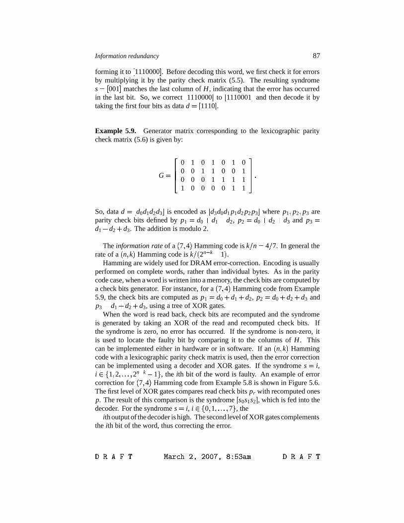
Information redundancy 87
forming it to ' 1110000 ) . Before decoding this word, we first check it for errorsby multiplying it by the parity check matrix (5.5). The resulting syndromes *æ' 001 ) matches the last column of H , indicating that the error has occurredin the last bit. So, we correct ' 1110000 ) to ' 1110001 ) and then decode it bytaking the first four bits as data d *æ' 1110 ) .Example 5.9. Generator matrix corresponding to the lexicographic paritycheck matrix (5.6) is given by:
G * |~~� 0 1 0 1 0 1 00 0 1 1 0 0 10 0 0 1 1 1 11 0 0 0 0 1 1
�\��� -So, data d *ð' d0d1d2d3 ) is encoded as ' d3d0d1 p1d2 p2 p3 ) where p1 ( p2 ( p3 areparity check bits defined by p1 * d0 5 d1 5 d2, p2 * d0 5 d2 5 d3 and p3 *d1 5 d2 5 d3. The addition is modulo 2.
The information rate of a % 7 ( 4 & Hamming code is k 8 n * 4 8 7. In general therate of a % n ( k & Hamming code is k 8p% 2n A k 2 1 & .
Hamming are widely used for DRAM error-correction. Encoding is usuallyperformed on complete words, rather than individual bytes. As in the paritycode case, when a word is written into a memory, the check bits are computed bya check bits generator. For instance, for a % 7 ( 4 & Hamming code from Example5.9, the check bits are computed as p1 * d0 5 d1 5 d2, p2 * d0 5 d2 5 d3 andp3 * d1 5 d2 5 d3, using a tree of XOR gates.
When the word is read back, check bits are recomputed and the syndromeis generated by taking an XOR of the read and recomputed check bits. Ifthe syndrome is zero, no error has occurred. If the syndrome is non-zero, itis used to locate the faulty bit by comparing it to the columns of H . Thiscan be implemented either in hardware or in software. If an % n ( k & Hammingcode with a lexicographic parity check matrix is used, then the error correctioncan be implemented using a decoder and XOR gates. If the syndrome s * i,i � P 1 ( 2 (R-R-R-I( 2n A k 2 1 S , the ith bit of the word is faulty. An example of errorcorrection for % 7 ( 4 & Hamming code from Example 5.8 is shown in Figure 5.6.The first level of XOR gates compares read check bits pr with recomputed onesp. The result of this comparison is the syndrome ' s0s1s2 ) , which is fed into thedecoder. For the syndrome s * i, i � P 0 ( 1 (R-R-R-I( 7 S , the
ith output of the decoder is high. The second level of XOR gates complementsthe ith bit of the word, thus correcting the error.
��������� � �����������������������! �"�$# ���������

88 FAULT TOLERANT DESIGN: AN INTRODUCTION
áú[IghVNXN[`bÉÉÉ
ÉÉÉÉÉÉÉ
ì oì o� ì qì q� ì7Ëì7Ë � �� o� q
CGDn ½� Ç
B � �� o� q� ���� ���
� Ë� ��Noì o�Fqì qì7Ë
��Va[!b;beVcb
Figure 5.6. Error-correcting circuit for an K 7 ü 4 L Hamming code.
Often, extended Hamming code rather than regular Hamming code is used,which allows not only the that single-bit errors can be corrected, but also thatdouble-bit errors can be detected. We describe this code in the next section.
4.8 Extended Hamming codesThe code distance of a Hamming code is three. If we add a parity check bit
to every codeword of a Hamming code, then the code distance increases to four.The resulting code is called extended Hamming code. It can correct single-biterrors and detect double-bit errors.
The parity check matrix for an extended % n ( k & Hamming code can be obtainedby first adding a zero column in front of a lexicographic parity check matrix ofan % n ( k & Hamming code, and then by attaching a row consisting of all 1’s asthe n 2 k 5 1th row of the resulting matrix. For example, the matrix H for anextended % 1 ( 1 & Hamming code is given by
H * � 0 11 1 � -
The matrix H for an extended % 3 ( 2 & Hamming code is given by
H * |� 0 0 1 10 1 0 11 1 1 1
�� -��������� � �����������������������! �"�$# ���������

Information redundancy 89
The matrix H for an extended % 7 ( 4 & Hamming code is given by
H *}|~~� 0 0 0 0 1 1 1 10 0 1 1 0 0 1 10 1 0 1 0 1 0 11 1 1 1 1 1 1 1
�\��� -If c *�' c1 ( c2 (R-R-R-h( cn ) is a codeword from an % n ( k & Hamming code, then c � *' c0 ( c1 ( c2 (R-R-R-`( cn ) is the corresponding extended codeword, where c0 * ∑n
i 9 1 ci
is the parity bit.
5. Cyclic codesCyclic codes are a special class of linear codes. Cyclic codes are used in
applications where burst errors can occur, in which a group of adjacent bits isaffected. Such errors are typical in digital communication as well as in storagedevices, such as discs and tapes. Scratch on a compact disk is one example ofa burst error. Two important classes of cyclic codes which we will considerare cyclic redundancy check (CRC) codes, used in modems and network pro-tocols and Reed-Solomon codes, applied in satellite communication, wirelesscommunication, compact disk players and DVDs.
5.1 DefinitionA linear code is called cyclic if ' cn A 1c0c1c2 -R-R- cn A 2 ) is a codeword whenever' c0c1c2 -R-R- cn A 2cn A 1 ) is also a codeword. So, any end-around shift of a codeword
of a cyclic code produces another codeword.When working with cyclic codes, it is convenient to think of words as poly-
nomials rather than vectors. For a binary cyclic code, the coefficients of thepolynomials are 0 or 1. For example, a data word ' d0d1d2 -R-R- dk A 1dk ) is repre-sented as a polynomial
d0 4 x0 5 d1 4 x1 5 d2 4 x2 5å-R-R-R5 dk A 1 4 xk A 1 5 dk 4 xk
where addition and multiplication is in the field Z2, i.e modulo 2. The degreeof a polynomial equals to its highest exponent. For example, a word [1011]corresponds to the polynomial 1 4 x0 5 0 4 x1 5 1 4 x2 5 1 4 x3 * 1 5 x2 5 x3 (leastsignificant bit on the left). The degree of this polynomial is 3.
Before continuing with cyclic codes, we first review the basics of polynomialarithmetics, necessary for understanding of encoding and decoding algorithms.
5.2 Polynomial manipulationIn this section we consider examples of polynomial multiplication and divi-
sion. All the operations are carried out in the field Z2, i.e. modulo 2.
��������� � �����������������������! �"�$# ���������

90 FAULT TOLERANT DESIGN: AN INTRODUCTION
Example 5.10. Compute % 1 5 x 5 x3 &�4 % 1 5 x2 & .% 1 5 x 5 x3 &�4·% 1 5 x2 &T* 1 5 x 5 x3 5 x2 5 x3 5 x5 * 1 5 x 5 x2 5 x5
Note, that x3 5 x3 * 0, since addition is modulo 2.
Example 5.11. Compute % 1 5 x3 5 x5 5 x6 &R8p% 1 5 x 5 x3 & .x3 5 x2 5 x 5 1
x3 5 x 5 1 3 x6 5 x5 5 x3 5 1x6 5 x4 5 x3
x5 5 x4 5 1x5 5 x3 5 x2
x4 5 x3 5 x2 5 1x4 5 x2 5 x
x3 5 x 5 1x3 5 x 5 1
0
So, 1 5 x 5 x3 divides 1 5 x3 5 x5 5 x6 without a reminder and the result is1 5 x 5 x2 5 x3.
For the decoding algorithm we also need to know how to perform arithmeticmodulo p % x & , where p % x & is a polynomial. To find f % x & mod p % x & , we dividef % x & by p % x & and take the remainder.
Example 5.12. Compute % 1 5 x2 5 x5 & mod % 1 5 x 5 x3 & .x3 5 x 5 1
x3 5 x 5 1 3 x5 5 x2 5 1x5 5 x3 5 x2
x3 5 1x3 5 x 5 1
x
So, % 1 5 x2 5 x5 & mod % 1 5 x 5 x3 &T* x.
5.3 Generator polynomialTo encode data in a cyclic code, the polynomial representing the data is
multiplied by a polynomial known as generator polynomial. The generatorpolynomial determines the properties of the resulting cyclic code. For example,suppose we encode the data [1011] using the generator polynomial g % x &Ð*��������� � �����������������������! �"�$# ���������

Information redundancy 91
1 5 x 5 x3 (least significant bit on the left). The polynomial representing thedata is d % x &1* 1 5 x2 5 x3. By computing g % x &�4 d % x & , we get 1 5 x 5 x2 5 x3 5x4 5 x5 5 x6. So, the codeword corresponding to the data [1011] is [1111111].
The choice of the generator polynomials is guided by the property that g % x &is the generator polynomial for a linear cyclic code of length n if and only ifg % x & divides 1 5 xn without a reminder.
If n is the length of the codeword, then the length of the encoded data word isk * n 2 deg % g % x &R& where deg % g % x &R& denotes the degree of the generator polyno-mial g % x & . A cyclic code with a generator polynomial of degree n 2 k is called% n ( k & cyclic code. An % n ( k & cyclic code can detect burst errors affecting n 2 kbits or less.
Example 5.13. Find a generator polynomial for a code of length n * 7 forencoding data of length k * 4.
We are looking for a polynomial of degree 7 2 4 * 3 which divides 1 5 x7
without a reminder. The polynomial 1 5 x7 can be factored as 1 5 x7 *ð% 1 5x 5 x3 &·% 1 5 x2 5 x3 &·% 1 5 x & , so we can choose either g % x &+* 1 5 x 5 x3 or g % x &+*1 5 x2 5 x3. Table 5.3 shows the cyclic code generated by g % x &¶* 1 5 x 5 x3.Since deg % g % x &R&1* 3, 3-bit burst errors can be detected by this code.
data codewordd0 d1 d2 d3 c0 c1 c2 c3 c4 c5 c6
0 0 0 0 0 0 0 0 0 0 00 0 0 1 0 0 0 1 1 0 10 0 1 0 0 0 1 1 0 1 00 0 1 1 0 0 1 0 1 1 10 1 0 0 0 1 1 0 1 0 00 1 0 1 0 1 1 1 0 0 10 1 1 0 0 1 0 1 1 1 00 1 1 1 0 1 0 0 0 1 11 0 0 0 1 1 0 1 0 0 01 0 0 1 1 1 0 0 1 0 11 0 1 0 1 1 1 0 0 1 01 0 1 1 1 1 1 1 1 1 11 1 0 0 1 0 1 1 1 0 01 1 0 1 1 0 1 0 0 0 11 1 1 0 1 0 0 0 1 1 01 1 1 1 1 0 0 1 0 1 1
Table 5.3. Defining table for (7,4) with the generator polynomial g K x L�M 1 � x � x3 .
��������� � �����������������������! �"�$# ���������

92 FAULT TOLERANT DESIGN: AN INTRODUCTION
Let C be an % n ( k & cyclic code generated by the generator polynomial g % x & .Codewords xig % x & are basis for C, since every codeword
d % x & g % x &1* d0g % x &75 d1xg % x &75å-R-R- dk A 1xk A 1g % x &is a linear combination of xig % x & . So, the following matrix G with rows xig % x &is a generator matrix for C:
G * |~~~~�g % x &xg % x &-R-R-
xk A 2g % x &xk A 1g % x &
�\����� * |~~~~�g0 g1 -R-R- gn A k 0 0 -R-R- 00 g0 g1 -R-R- gn A k 0 -R-R- 0-R-R-0 0 0 g0 g1 -R-R- gn A k 00 0 0 0 g0 g1 -R-R- gn A k
�\����� -Every row of G is a right cyclic shift of the first row. This generator matrix
leads to a simple encoding algorithm using polynomial multiplication by g % x & .Example 5.14. If C is a binary cyclic code with the generator polynomialg % x &t* 1 5 x 5 x3, then the generator matrix is given by:
G * |~~� 1 1 0 1 0 0 00 1 1 0 1 0 00 0 1 1 0 1 00 0 0 1 1 0 1
�\��� -5.4 Parity check polynomial
Given a cyclic code C with the generator polynomial g % x & , the polynomialh % x & determined by
g % x & h % x &t* 1 5 xn
is the check polynomial of C. Since codewords of a cyclic code are multiplesof g % x & , for every codeword c % x &¶� C, it is hold that
c % x & h % x &1* d % x & g % x & h % x &¶* d % x &·% 1 5 xn &+* 0 mod 1 5 xn -A parity check matrix H contains as its first row the coefficient of h % x & ,
starting from the most significant one. Every following row of H is a rightcyclic shift of the first row.
H * |~~~~�hk hk A 1 -R-R- h0 0 0 -R-R- 00 hk hk A 1 -R-R- h0 0 -R-R- 0-R-R-0 -R-R- 0 hk hk A 1 -R-R- h0 00 -R-R- 0 0 hk hk A 1 -R-R- h0
�\����� -��������� � �����������������������! �"�$# ���������

Information redundancy 93
Example 5.15. Suppose C is a binary cyclic code with the generator polyno-mial g % x &�* 1 5 x 5 x3. Let us compute its check polynomial.
There are three factors of 1 5 x7: 1 5 x ( 1 5 x 5 x3 and 1 5 x2 5 x3. Thus,h % x &t*�% 1 5 x2 5 x3 &·% 1 5 x &t* 1 5 x 5 x2 5 x4. The corresponding parity checkmatrix is given by
H * |� 1 0 1 1 1 0 00 1 0 1 1 1 00 0 1 0 1 1 1
�� - (5.7)
5.5 Syndrome polynomialSince cyclic codes are linear codes, we can use the parity check polyno-
mial to detect errors which possibly occurred in a codeword c % x & during datatransmission or storage. We define
s % x &�* h % x & c % x & mod 1 5 xn
to be the syndrome polynomial. Since g % x & h % x &Ð* 1 5 xn, syndrome can becomputed by dividing the c % x & by g % x & . If the reminder s % x & is zero, then c % x &is a codeword. Otherwise, there is an error in c % x & .5.6 Implementation of polynomial division
The polynomial division can be implemented by linear feedback shift reg-isters (LFSR). Logic diagram of an LFSR for the generator polynomial ofdegree r * n 2 k is shown in Figure 5.7. It consists of a simple shift registerand binary-weighted modulo 2 sums with feedback connections. Weights g i,i �uP 0 ( 1 (R-R-R-I( r 2 1 S , are the coefficients of the generator polynomial g % x &Õ*g0x0 5 g2x1 5 -R-R- gnxn. Each gi is either 0, meaning “no connection”, or 1,meaning “connection”. An exception is gr which is always 1 and therefore isalways connected.
If the input polynomial is c % x & , then the LFSR divides c % x & by the generatorpolynomial g % x & , resulting in the quotient d % x & and the reminder s % x & . Thecoefficients ' s0s1 -R-R- sr ) of the syndrome polynomial are contained in the registerafter the division is completed. If syndrome is zero, then c % x & is a codewordand d % x & is valid data. If ' s0s1 -R-R- sr ) matches one of the columns of parity checkmatrix H , then a single-bit error has occurred. The bit position of the errorcorresponds to the position of the matching column in H , so the error can becorrected. If the syndrome is not zero and is not equal to any of the columns ofH , then a multiple-bit error has occurred which cannot be corrected.
Example 5.16. As an example, consider the logic circuit shown in Figure 5.8.It implements LFSR for the generator polynomial g % x &¶* 1 5 x 5 x3. Let s �i��������� � �����������������������! �"�$# ���������

94 FAULT TOLERANT DESIGN: AN INTRODUCTION
� � � �� � � o � q � é o �
í`í`íFigure 5.7. Logic diagram of a Linear Feedback Shift Register (LFSR).
denotes the next state value of the register cell si. Then, the state values of theLFSR in Figure 5.8 are given by
s �0 * s2 5 c % x &s �1 * s0 5 s2
s �2 * s1
� � � o � qÉÉ� ? Ê @ �6? Ê @ghZ\V¨g��
Figure 5.8. Implementation of the decoding circuit for cyclic code with the generator polyno-mial g K x L7M 1 � x � x3 .
Suppose the word to be decoded is ' 1010001 ) , i.e. 1 5 x2 5 x6. Table 5.4shows the values of the register. This word is fed into the LFSR with the mostsignificant bit first. The first bit of quotient (most significant one) appears atthe output at 4th clock cycle. In general, the first bit of quotient comes outat the clock cycle r 5 1 for an LFSR of size r * n 2 k. After the division iscompleted at cycle 7 (cycle n for the general case), the state of the register is' 000 ) , so ' 1010001 ) is a codeword and the quotient ' 1101 ) is valid data. We canverify the obtained result by dividing 1 5 x2 5 x6 by 1 5 x 5 x3. The quotient is1 5 x 5 x3, which is indeed ' 1101 ) .Example 5.17. Next, suppose that a single-bit error has occurred in the 4thbit of codeword ' 1010001 ) , and a word ' 1011001 ) is received instead. Table 5.5illustrates the decoding process. As we can see, after the division is completed,the registers contain the reminder ' 110 ) , which matches the 4th column of theparity check matrix H in (5.7).
��������� � �����������������������! �"�$# ���������
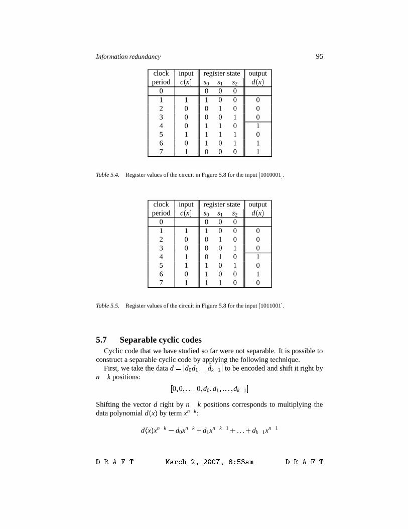
Information redundancy 95
clock input register state outputperiod c % x & s0 s1 s2 d % x &
0 0 0 01 1 1 0 0 02 0 0 1 0 03 0 0 0 1 04 0 1 1 0 15 1 1 1 1 06 0 1 0 1 17 1 0 0 0 1
Table 5.4. Register values of the circuit in Figure 5.8 for the input � 1010001 � .clock input register state outputperiod c % x & s0 s1 s2 d % x &
0 0 0 01 1 1 0 0 02 0 0 1 0 03 0 0 0 1 04 1 0 1 0 15 1 1 0 1 06 0 1 0 0 17 1 1 1 0 0
Table 5.5. Register values of the circuit in Figure 5.8 for the input � 1011001 � .
5.7 Separable cyclic codesCyclic code that we have studied so far were not separable. It is possible to
construct a separable cyclic code by applying the following technique.First, we take the data d *�' d0d1 -R-R- dk A 1 ) to be encoded and shift it right by
n 2 k positions: ' 0 ( 0 (R-R-R-!( 0 ( d0 ( d1 (R-R-R-h( dk A 1 )Shifting the vector d right by n 2 k positions corresponds to multiplying thedata polynomial d % x & by term xn A k:
d % x & xn A k * d0xn A k 5 d1xn A k � 1 5å-R-R-h5 dk A 1xn A 1
��������� � �����������������������! �"�$# ���������
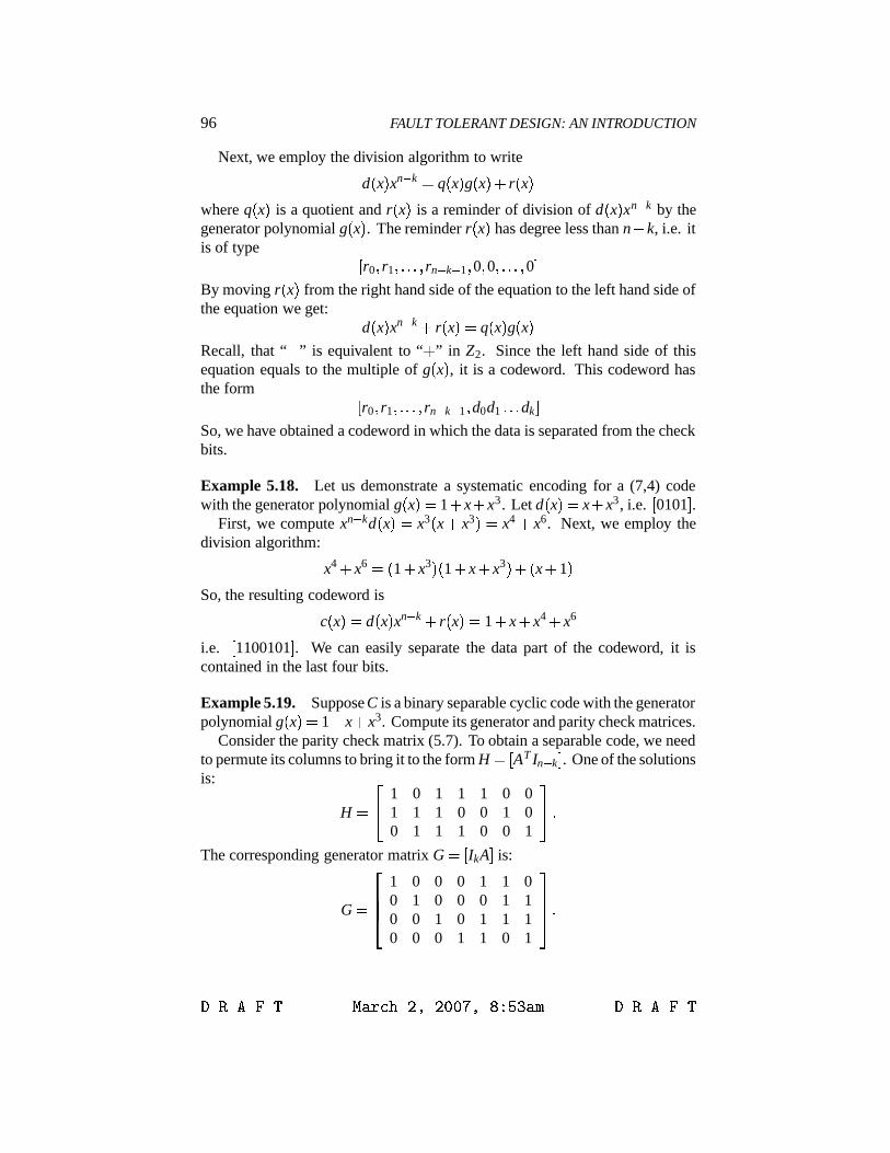
96 FAULT TOLERANT DESIGN: AN INTRODUCTION
Next, we employ the division algorithm to write
d % x & xn A k * q % x & g % x &75 r % x &where q % x & is a quotient and r % x & is a reminder of division of d % x & xn A k by thegenerator polynomial g % x & . The reminder r % x & has degree less than n 2 k, i.e. itis of type ' r0 ( r1 (R-R-R-h( rn A k A 1 ( 0 ( 0 (R-R-R-!( 0 )By moving r % x & from the right hand side of the equation to the left hand side ofthe equation we get:
d % x & xn A k 5 r % x &�* q % x & g % x &Recall, that “ 2 ” is equivalent to “ 5 ” in Z2. Since the left hand side of thisequation equals to the multiple of g % x & , it is a codeword. This codeword hasthe form ' r0 ( r1 (R-R-R-h( rn A k A 1 ( d0d1 -R-R- dk )So, we have obtained a codeword in which the data is separated from the checkbits.
Example 5.18. Let us demonstrate a systematic encoding for a (7,4) codewith the generator polynomial g % x &+* 1 5 x 5 x3. Let d % x &+* x 5 x3, i.e. ' 0101 ) .
First, we compute xn A kd % x &¶* x3 % x 5 x3 &Ã* x4 5 x6. Next, we employ thedivision algorithm:
x4 5 x6 *�% 1 5 x3 &·% 1 5 x 5 x3 &75% x 5 1 &So, the resulting codeword is
c % x &t* d % x & xn A k 5 r % x &T* 1 5 x 5 x4 5 x6
i.e. ' 1100101 ) . We can easily separate the data part of the codeword, it iscontained in the last four bits.
Example 5.19. Suppose C is a binary separable cyclic code with the generatorpolynomial g % x &�* 1 5 x 5 x3. Compute its generator and parity check matrices.
Consider the parity check matrix (5.7). To obtain a separable code, we needto permute its columns to bring it to the form H *Q' AT In A k ) . One of the solutionsis:
H * |� 1 0 1 1 1 0 01 1 1 0 0 1 00 1 1 1 0 0 1
�� -The corresponding generator matrix G *�' IkA ) is:
G * |~~� 1 0 0 0 1 1 00 1 0 0 0 1 10 0 1 0 1 1 10 0 0 1 1 0 1
�\��� -��������� � �����������������������! �"�$# ���������

Information redundancy 97
Since encoding of a separable cyclic code involves division, it can be imple-mented using an LFSR identical to the one used for decoding. The multiplica-tion by xn A k is done by shifting the data right by n 2 k positions. After the lastbit of d % x & has been fed in, the LFSR contains the reminder of division of inputpolynomial by g % x & . By subtracting this reminder from xn A kd % x & we obtain theencoded word.
5.8 CRC codes
Cyclic redundancy check (CRC) codes are separable cyclic codes with spe-cific generator polynomials, chosen to provide high error detection capabilityfor data transmission and storage. Common generator polynomials for CRC are:
CRC-16: 1 5 x2 5 x15 5 x16
CRC-CCITT: 1 5 x5 5 x12 5 x16
CRC-32:1 5 x 5 x2 5 x4 5 x7 5 x8 5 x10 5 x11 5 x12 5 x16 5 x22 5 x23 5 x26 5 x32
CRC-16 and CRC-CCITT are widely used in modems and network protocolsin the USA and Europe, respectively, and give adequate protection for mostapplications. An attractive feature of CRC-16 and CRC-CCITT is the smallnumber of non-zero terms in their polynomials (just four). This is an advantagebecause LFSR required to implement encoding and decoding is simpler forgenerator polynomials with the small number of terms. Applications that needextra protection, such as Department of Defense applications, use CRC-32.
The encoding and decoding is done either in software, or in hardware, usingthe procedure from Section 5.7. To perform an encoding, data polynomial isfirst shifted right by deg % g % x &R& bit positions, and then divided by the genera-tor polynomial. The coefficients of the remainder form the check bits of theCRC codeword. The number check bits equals to the degree of the generatorpolynomial. So, an CRC detects all burst errors of length less or equal thandeg % g % x &R& . An CRC also detects many errors which are larger than deg % g % x &R& .For example, apart from detecting all burst errors of length 16 or less, CRC-16and CRC-CCITT are also capable to detect 99.997% of burst errors of length17 and 99.9985 burst errors of length 18.
5.9 Reed-Solomon codes
Reed-Solomon (RS) codes are a class of separable cyclic codes used to correcterrors in a wide range of applications including storage devices (tapes, com-pact discs, DVDs, bar-codes), wireless communication (cellular telephones, mi-crowave links), satellite communication, digital television, high-speed modems(ADSL, xDSL).
��������� � �����������������������! �"�$# ���������

98 FAULT TOLERANT DESIGN: AN INTRODUCTION
The encoding for Reed-Solomon code is done similarly to the proceduredescribed in Section 5.7. The codeword is computed by shifting the data rightn 2 k positions, dividing it by the generator polynomial and then adding theobtained reminder to the shifted data. A key difference is that groups of m bitsrather than individual bits are used as symbols of the code. Usually m * 8, i.e.a byte. The theory behind is a field Zm
2 of degree m over P 0 ( 1 S . The elementsof such a field are m-tuples of 0 and 1, rather than just 0 and 1.
An encoder for an Reed-Solomon code takes k data symbols of s bits eachand computes a codeword containing n symbols of m bits each. The maximumcodeword length is related to m as n * 2m 2 1. A Reed-Solomon code cancorrect up to
Ín 2 k ÎH8 2 symbols that contain errors.
For example, a popular Reed-Solomon code is RS(255,223) where symbolsare a byte (8-bit) long. Each codeword contains 255 bytes, of which 223 bytesare data and 32 bytes are check symbols. So, n * 255 ( k * 223 and thereforethis code can correct up to 16 bytes containing errors. Note, that each of these16 bytes can have multiple bit errors.
Decoding of Reed-Solomon codes is performed using an algorithm designedby Berlekamp. The popularity of Reed-Solomon codes is due to a large extentto the efficiency this algorithm. Berlekamp’s algorithm was used by Voyager IIfor transmitting pictures of the outer space back to Earth. It is also a basis fordecoding CDs in players. Many additional improvements were done over theyears to make Reed-Solomon code practical. Compact discs, for example, usea modified version of RS code called cross-interleaved Reed-Solomon code.
6. Unordered codesUnordered codes are designed to detect unidirectional errors. A unidirec-
tional error is an error which changes either 0’s of the word to 1, or 1’s ofthe word to 0, but not both. An example of a unidirectional error is an errorchanging a word [1011000] to the word [0001000]. It is possible to apply aspecial design technique to ensure that most of the faults occurring in a logiccircuit cause only unidirectional errors on the output. For example, considerthe logic circuit shown in Figure 5.9. If a single stuck-at fault occurs at any ofthe lines in the circuit, it will cause a unidirectional error in the output word' f1 f2 f3 ) .
The name of unordered codes originates from the following. We say thattwo binary n-tuples x *s% x1 (R-R-R-h( xn & and y *ð% x1 (R-R-R-h( xn & are ordered if eitherxi 0 yi for all i � P 1 ( 2 (R-R-R-I( n S , or xi ù yi for all i. For example if x *�' 0101 ) andy *æ' 0000 ) then x and y are ordered, namely x ù y. A unidirectional code is acode satisfying the property that any two of its codewords are unordered.
The ability of unordered codes to detect all unidirectional errors is directlyrelated to the above property. A unidirectional error always changes a wordx to a word y which is either smaller or greater than x. A unidirectional error
��������� � �����������������������! �"�$# ���������

Information redundancy 99
ÉÉÉ ÉÉÉÊ qÊ7ËÊ �Ê o
Ê Ò Ì qÌo
Ì ËFigure 5.9. Logic diagram of a circuit in which any single stuck-at fault cause a unidirectionalerror on the output.
cannot change x to a word which is not ordered with x. Therefore, if any twoof its codewords of a code are unordered, then a unidirectional error will nevermap a codeword to another codeword, and thus will be detected.
In this section we describe two unordered codes: m-of-n codes and Bergercodes.
6.1 M-of-n codesA m-of-n code consists of all n-bit words with exactly m 1’s. Any k-bit
unidirectional error forces the affected codeword to have either m 5 k of m 2 k1’s, and thus detected.
An easy way to construct an m-of-n code is to take the original k bits of dataand append k bits so that the resulting 2k-bit code word has exactly k 1’s. Forexample, the 3-of-6 code is shown in Table 5.6. All codewords have exactlythree 1’s.
data codewordd0 d1 d2 c0 c1 c2 c3 c4 c5
0 0 0 0 0 0 1 1 10 0 1 0 0 1 1 1 00 1 0 0 1 0 1 0 10 1 1 0 1 1 1 0 01 0 0 1 0 0 0 1 11 0 1 1 0 1 0 1 01 1 0 1 1 0 0 0 11 1 1 1 1 1 0 0 0
Table 5.6. Defining table for 3-of-6 code.
��������� � �����������������������! �"�$# ���������

100 FAULT TOLERANT DESIGN: AN INTRODUCTION
An obvious disadvantage of an 2k-of-k is its low information rate of 1/2.An advantage of this code is its separability, which simplifies the encoding anddecoding procedures. A more efficient m-of-n code, with higher informationrate can be constructed, but then the separable nature of the code is usually lost.Non-separability makes the encoding, decoding and error detection proceduresmore difficult.
6.2 Berger codesCheck bits in a Berger code represent the number of 1’s in the data word. A
Berger code of length n has k data bits and m check bits, where m *æ÷ log2 % k 5 1 &;øand n * k 5 m. A codeword is created by complementing the m-bit binaryrepresentation of the number of 1’s in the encoded word. An example of Bergercode for 4-bit data is shown in Table 5.7.
data codewordd0 d1 d2 d3 c0 c1 c2 c3 c4 c5 c6
0 0 0 0 0 0 0 0 1 1 10 0 0 1 0 0 0 1 1 1 00 0 1 0 0 0 1 0 1 1 00 0 1 1 0 0 1 1 1 0 10 1 0 0 0 1 0 0 1 1 00 1 0 1 0 1 0 1 1 0 10 1 1 0 0 1 1 0 1 0 10 1 1 1 0 1 1 1 1 0 01 0 0 0 1 0 0 0 1 1 01 0 0 1 1 0 0 1 1 0 11 0 1 0 1 0 1 0 1 0 11 0 1 1 1 0 1 1 1 0 01 1 0 0 1 1 0 0 1 0 11 1 0 1 1 1 0 1 1 0 01 1 1 0 1 1 1 0 1 0 01 1 1 1 1 1 1 1 0 1 1
Table 5.7. Defining table for Berger code for 4-bit data.
The primary advantages of a Berger code are that it is a separable code andthat it detects all unidirectional multiple errors. It is shown that Berger code isthe most compact code for this purpose. The information rate of a Berger codefor m-bit data is k 8p%»÷ k 5�÷ log2 % k 5 1 &;øH& . Table 5.8 shows how the informationrate grows as the size of encoded data increases. For data of small size, the
��������� � �����������������������! �"�$# ���������

Information redundancy 101
redundancy of a Berger code is high. However, as k increases, the number ofcheck bits drops substantially. The Berger codes with k * 2m 2 1 are calledmaximal length Berger codes.
number of number or informationdata bits check bits rate
4 3 0.578 4 0.67
16 5 0.7632 6 0.8464 7 0.90128 8 0.94
Table 5.8. Information rate of different Berger codes.
7. Arithmetic codesArithmetic codes are usually used for detecting errors in arithmetic opera-
tions, such as addition or multiplication. The data representing the operands,say b and c, is encoded before the operation is performed. The operation iscarried out on the resulting codewords A % b & and A % c & . After the operation, thecodeword A % b &�� A % c & representing the result of the operation “ � ” is decodedand checked for errors.
An arithmetic code relies on the property of invariance with respect to theoperation “ � ”:
A % b � c &T* A % b & � A % c &Invariance guarantees that the operation “ � ” on codewords A % b & and A % c & givesus the same result as A % b � c & . So, if no error has occurred, decoding A % b � c &gives us b � c, the result of the operation “ � ” on b and c.
Two common types of arithmetic codes are AN-codes and residue codes.
7.1 AN-codesAN-code is the simplest representative of arithmetic codes. The codewords
are obtained by multiplying data words N by some constant A. For example,if the data is of length two, namely [00], [01], [10], [11], then the 3N-code is[0000], [0011], [0110], [1001]. Each codeword is computed by multiplying adata word by 3. And vice versa, to decode a codeword, we divide it by 3. Ifthere is no reminder, no error has occurred. AN-codes are non-separable codes.
��������� � �����������������������! �"�$# ���������

102 FAULT TOLERANT DESIGN: AN INTRODUCTION
The AN-code is invariant with respect to addition and subtraction, but notto multiplication and division. For example, clearly 3 % a 4 b & y* 3a 4 3b for allnon-zero a, b.
The constant A determines the information rate of the code and its error de-tection capability. For binary codes, A should not be a power of two. This isbecause single-bit errors cause multiplication or division of the original code-word by 2r, where r is the position of the affected bit. Therefore, the resultingword is a codeword and the error cannot be detected.
7.2 Residue codesResidue codes are separable arithmetic codes which are created by computing
a residue for data and appending it to the data. The residue is generated bydividing a data by an integer, called modulus. Decoding is done by simplyremoving the residue.
Residue codes are invariant with respect to addition, since% b 5 c & mod m * b mod m 5 c mod m
where b and c are data words and m is modulus. This allows us to handleresidues separately from data during addition process. The value of the modulusdetermines the information rate and the error detection capability of the code.
A variation of residue codes are inverse residue code, where an inverse ofthe residue, rather than the residue itself, is appended to the data. These codesare shown to have better fault detecting capabilities for common-mode faults.
8. Problems5.1. Give an example of a binary code of length 4 and of size 6. How many
words are contained in the codespace of your code?
5.2. Why is separability of a code considered to be a desirable feature?
5.3. Define the information rate. How is the information rate related to redun-dancy?
5.4. What is the main difference in the objectives of encoding for the codingtheory and the cryptography?
5.5. What is the maximum Hamming distance between two words in the codespaceP 0 ( 1 S 4?
5.6. Consider the code C *�P 01100101110 ( 10010110111 ( 01010011001 S .(a) What is the code distance of C?
(b) How many errors can be detected/corrected by code C?
��������� � �����������������������! �"�$# ���������

Information redundancy 103
5.7. How would you generalize the notions of Hamming distance and code dis-tance to ternary codes using P 0 ( 1 ( 2 S as valid symbols? Find a generalizationwhich preserves the following two properties: To be able to correct ε-digiterrors, a ternary code should have the code distance of at least 2ε 5 1. Tobe able to detect ε-digit errors, the ternary code distance should be at leastε 5 1.
5.8. Prove that, for any n ¹ 1, a parity code of length n has code distance two.
5.9. (a) Construct an even parity code C for 3-bit data.
(b) Suppose the word (1101) is received. Assuming single bit error, whatare the codewords that have possibly been transmitted?
5.10. Draw a gate-level logic circuit of an odd parity generation circuit for 5-bitdata. Limit yourself to use of two-input gates only.
5.11. How would you generalize the notion of parity for ternary codes? Give anexample of a ternary parity code for 3-digit data, satisfying your definition.
5.12. Construct the parity check matrix H and the generator matrix G for a linearcode for 4-bit data which can:
(a) detect 1 error
(b) correct 1 error
(c) correct 1 error and detect one additional error.
5.13. Construct the parity check matrix H and the generator matrix G for a linearcode for 5-bit data which can:
(a) detect 1 error
(b) correct 1 error
(c) correct 1 error and detect one additional error.
5.14. (a) Construct the parity check matrix H and the generator matrix G of aHamming code for 11-bit data.
(a) Find whether you can construct a Hamming code for data of lengths 1 ( 2and 3. Construct the parity check matrix H and the generator matrix Gfor whose lengths for which it is possible.
5.15. The parity code is a linear code, too. Construct the parity check matrix Hand the generator matrix G for a parity code for 4-bit data.
5.16. Find the generator matrix for the (7,4) cyclic code C with the generatorpolynomial 1 5 x2 5 x3. Prove that C is a Hamming code.
��������� � �����������������������! �"�$# ���������

104 FAULT TOLERANT DESIGN: AN INTRODUCTION
5.17. Find the generator matrix for the (15,11) cyclic code C with the generatorpolynomial 1 5 x 5 x4. Prove that C is a Hamming code.
5.18. Compute the check polynomial for the (7,4) cyclic code with the generatorpolynomial g % x &t* 1 5 x2 5 x3.
5.19. Let C be and % n ( k & cyclic code. Prove that the only burst errors of lengthn 2 k 5 1 that are codewords (and therefore not detectable errors) are shiftsof scalar multiples of the generator polynomial.
5.20. Suppose you use a cyclic code generated by the polynomial g % x &T* 1 5 x 5 x3.You have received a word c % x &1* 1 5 x 5 x4 5 x5. Check whether an errorhas occur during transmission.
5.21. Develop an LFSR for decoding of 4-bit data using the generator polynomialg % x &+* 1 5 x4. Show the state table for the word c % x &+* x7 5 x6 5 x5 5 x3 5 1(as the one in Table 5.4). Is c % x & a valid codeword?
5.22. Construct a separable cyclic code for 4-bit data generated by the polynomialg % x &t* 1 5 x 5 x4. What code distance has the resulting code?
5.23. (a) Draw an LFSR decoding circuit for CRC codes with the following gen-erator polynomials:
CRC 2 16 : 1 5 x2 5 x15 5 x16
CRC 2 CCITT : 1 5 x5 5 x12 5 x16
You may use " -R-R- " between the registers 2 and 15 in the 1st polynomialand 5 and 12 in the second, to make the picture shorter.
(b) Use the first generator polynomial for encoding the data 1 5 x3 5 x4.
(c) Suppose that the error 1 5 x 5 x2 is added to the codeword you obtainedin the previous task. Check whether this error will be detected or not.
5.24. Construct a Berger code for 3-bit data. What code distance has the resultingcode?
5.25. Suppose we know that the original 4-bit data words will never include theword 0000. Can we reduce the number of check bits required for a Bergercode and still cover all unidirectional errors?
5.26. Suppose we encoded 8-bit data using a Berger code.
(a) How many check bits are required?
(b) Take one codeword c and list all possible unidirectional error which canaffect c.
��������� � �����������������������! �"�$# ���������

Information redundancy 105
5.27. (a) Construct 3N arithmetic code for 3-bit data.
(b) Give an example of a fault which is detected by such a code and anexample a of fault which is not detected by such a code.
5.28. Consider the following code C:
0 0 0 0 0 00 0 0 1 0 10 0 1 0 1 00 0 1 1 1 10 1 0 1 0 00 1 1 0 0 10 1 1 1 1 01 0 0 0 1 1
(a) What kind of code is this?
(b) Is it a separable code?
(c) Which is the code distance of C?
(d) What kind of faults can it detect/correct?
(e) How are encoding and decoding done for this code? (describe in words)
(f) How error is detection done for this code? (describe in words)
5.29. Consider the following code C:
0 0 0 0 0 00 0 0 0 1 10 0 0 1 1 00 0 1 0 0 10 0 1 1 0 00 0 1 1 1 10 1 0 0 1 00 1 0 1 0 10 1 1 0 0 00 1 1 0 1 10 1 1 1 1 01 0 0 0 0 11 0 0 1 0 01 0 0 1 1 11 0 1 0 1 01 0 1 1 0 1
(a) What kind of code is this?
��������� � �����������������������! �"�$# ���������

106 FAULT TOLERANT DESIGN: AN INTRODUCTION
(b) Is it a separable code?
(c) Which is the code distance of C?
(d) What kind of faults can it detect/correct?
(e) How are encoding and decoding done for this code? (describe in words)
(f) How is error detection done for this code? (describe in words)
5.30. Consider the following code:
0 0 0 1 1 10 0 1 1 1 00 1 0 1 0 10 1 1 1 0 01 0 0 0 1 11 0 1 0 1 01 1 0 0 0 11 1 1 0 0 0
(a) What kind of code is this?
(b) Is it a separable code?
(c) Which is the code distance of C?
(d) What kind of faults can it detect/correct?
(e) Invent and draw a circuit (gate-level) for encoding of 3-bit data in thiscode. Your circuit should have 3 inputs for data bits and 6 outputs forcodeword bits.
(f) How would you suggest to do error detection for this code? (describein words).
<
5.31. Develop a scheme for active hardware redundancy (either standby sparingor pair-and-a-spare) employing error detection code of your choice for 1-biterror detection.
��������� � �����������������������! �"�$# ���������

Chapter 6
TIME REDUNDANCY
1. IntroductionSpace redundancy techniques discussed so far impact physical entities like
cost, weight, size, power consumption, etc. In some applications extra time isof less importance than extra hardware.
Time redundancy is achieved by repeating the computation or data trans-mission and comparing the result to a stored copy of the previous result. Ifthe repetition is done twice, and if the fault which has occurred is transient,then the stored copy will differ from the re-computed result, so the fault will bedetected. If the repetition is done three or more times, a fault can be corrected.In this section, we show that time redundancy techniques can also be used fordetecting permanent faults.
Apart from detection and correction of faults, time redundancy is useful fordistinguishing between transient and permanent faults. If the fault disappearsafter the re-computation, it is assumed to be transient. In this case the hardwaremodule is still usable and it would be a waste of resources to switch it off theoperation.
2. Alternating logicThe alternating logic time redundancy scheme was developed by Reynolds
and Metze in 1978. It has been applied to permanent fault detection in digitaldata transmission and in digital circuits.
Suppose the data is transmitted over a parallel bus as shown in Figure 6.1.At time t0, the original data is transmitted. Then, the data is complemented andre-transmitted at time t0 5 ∆. The two results are compared to check whetherthey are complements of each other. Any disagreement indicates a fault. Sucha scheme is capable of detecting permanent stuck-at faults at the bus lines.
��������� � �����������������������! �"�$# ���������

108 FAULT TOLERANT DESIGN: AN INTRODUCTION
!#"� $� %Ý ØØ & "
' &Þ&Ý#(& "= �= � ë*) CB C
CBB= � ë+) = �B CBB CBÑÑÑ ÑÑÑÑÑÑ ÑÑÑÑÑÑi<�;Y7g��-, © � B
Figure 6.1. Alternating logic time redundancy scheme.
Alternating logic concept can be used for detecting fault in logic circuitswhich implement self-dual functions. A dual of a function f % x1 ( x2 (R-R-R-!( xn & isdefined as
fd % x1 ( x2 (R-R-R-h( xn &+* f � % x �1 ( x �2 (R-R-R-h( x �n &!(where � denotes the complement. For example, a 2-variable AND f % x1 ( x2 &�*x1 4 x2 is dual of a 2-variable OR % x1 ( x2 &T* x1 5 x2, and vice versa. A functionin said to be self-dual if it is equal to its dual f * fd . So, the value of a self-dual function f for the input assignment x1 ( x2 (R-R-R-h( xn equals to the value ofthe complement of f for the input assignment x �1 ( x �2 (R-R-R-h( x �n. Examples of self-dual functions are sum and carry-out output functions of a full-adder (Figure6.2). The sum s % a ( b ( cin &t* a . b . cin, where ” . ” is an XOR. The carry-outÉ ÉÉÉ É
É /��0 1 �� Â;Å!¢i�, © , CFigure 6.2. Logic diagram of a full-adder.
cout % a ( b ( cin &1* ab 5 % a . b & cin . Table 6.1 shows the defining table for s andcout . It is easy to see that the property f % x1 ( x2 (R-R-R-h( xn &�* f � % x �1 ( x �2 (R-R-R-`( x �n & holdsfor both functions.
For a circuit implementing a self-dual function, the application of an input as-signment % x1 ( x2 (R-R-R-`( xn & followed by the input assignment % x �1 ( x �2 (R-R-R-h( x �n & shouldproduce output values which are complements of each other, unless the circuithas a fault. So, a fault can be detected by finding an input assignment for whichf % x1 ( x2 (R-R-R-h( xn &�* f % x �1 ( x �2 (R-R-R-h( x �n & . For example, a stuck-at-1 fault marked inFigure 6.2 can be detected by applying the input assignment % a ( b ( cin &�*�% 100 & ,followed by the complemented assignment % 011 & . In a fault-free full-adder
��������� � �����������������������! �"�$# ���������

Time redundancy 109
a b cin s cout
0 0 0 0 00 0 1 1 00 1 0 1 00 1 1 0 11 0 0 1 01 0 1 0 11 1 0 0 11 1 1 1 1
Table 6.1. Defining table for a full-adder.
s % 100 &�* 1, cout % 100 &+* 0 and s % 011 &+* 0, cout % 011 & * 1. However, in presenceof the marked fault s % 100 &Ã* 1, cout % 100 &Ã* 1 and s % 011 &Ã* 0, cout % 011 &Ã* 1.Since cout % 100 &�* cout % 011 & , the fault is detected.
If the function f % x1 ( x2 (R-R-R-h( xn & realized by the circuit is not self-dual, then itcan be transformed to a self-dual function of n 5 1-variables, defined by
fsd * xn � 1 f 5 x �n � 1 fd
The new variable xn � 1 is a control variable determining whether the value of f orfd appears on the output. Clearly, such a function fsd produces complementedvalues for complemented inputs. A drawback of this technique is that the circuitimplementing fsd can be twice larger than the circuit implementing f .
3. Recomputing with shifted operandsRecomputing with shifted operands (RESO) time redundancy technique was
developed by Patel and Fung in 1982 for on-line fault detection in arithmeticlogic units (ALUs) with bit-sliced organization.
At time t0, the bit slice i of a circuit performs a computation. Then, the datais shifted left and the computation is repeated at time t0 5 δ. The shift operandcan be either arithmetic or logical shift. After the computation, the result isshifted right. The two results are compared. If there is no error, they are thesame. Otherwise, they disagree in either the ith, or % i 2 1 & th, or both bits.
The fault detection capability of RESO depends on the amount of shift. Forexample, for a bit-sliced ripple-carry adder, 2-bit arithmetic shift is required toguarantee the fault detection. A fault in the ith bit of a slice can have one of thethree effects:
1 The sum bit is erroneous. Then, the incorrect result differs form the correctone by either 2 2i (if the sum is 0), or by 5 2i (if the sum is 1).
��������� � �����������������������! �"�$# ���������

110 FAULT TOLERANT DESIGN: AN INTRODUCTION
2 The carry bit is erroneous. Then, the incorrect result differs from the correctone by either 2 2i � 1 (if the carry is 0), or by 5 2i � 1 (if the carry is 1).
3 Both, sum and carry bits, are erroneous. Then, we have four possibilities
sum is 0, carry is 0: 2 3 4 2i;
sum is 0, carry is 1: 5 2i;
sum is 1, carry is 0: 2 2i;sum is 1, carry is 1: 5 3 4 2i;
Summarizing, if the operands are not shifted, then the erroneous result differsfrom the correct one by one of the following values: P 0 ( 2i ( 2i � 1 ( 3 4 2i � 1 S .
A similar analysis can be done to show that if the operands are shifted leftby two bits, then the erroneous result differs from the correct one by one of thefollowing values: P 0 ( 2i A 1 ( 2i A 2 ( 3 4 2i A 2 S . So, results of non-shifted and shiftedcomputations cannot agree unless they are both correct.
A primary problem with RESO technique is the additional hardware requiredto store the shifted bits.
4. Recomputing with swapped operandsRecomputing with swapped operands (RESWO) is another time redundancy
technique, introduced by Johnson in 1988. In RESWO, both operands are split-ted into two halves. During the first computation, the operands are manipulatedas usual. The second computation is performed with the lower and the upperhalves of operands swapped.
RESWO technique can detect faults in any single bit slice. For example,consider a bit-sliced ripple-carry adder with n-bit operands. Suppose the lowerhalf of an operand contains the bits from 0 to r * n 8 2 and the upper half containsthe bits from r 5 1 to n 2 1. During the first computation, if the sum and carrybits from slice i are faulty, then the resulting sum differs from the correct oneby 2i and 2i � 1, respectively. If both, the sum and the carry are faulty, then theresult differs from the correct one by 2i2i � 1, respectively. So, if the operandshalf are not swapped, a faulty bit slice i cause the result to disagree from thecorrect result by one of the values P 0 ( 2i ( 2i � 1 ( 2i2i � 1 S . If i 0 r, the result ofthe re-computation with the lower and the upper halves of operands swappeddiffers from the correct result by one of the values P 0 ( 2i A r ( 2i A r A 1 ( 2i A r2i A r A 1 S .So, results of non-swapped and swapped computations cannot agree unless theyare both correct.
5. Recomputing with duplication with comparisonRecomputing using duplication with comparison (REDWC) technique com-
bines hardware redundancy with time redundancy. An n-bit operation is per-formed by using two n 8 2-bit devices twice. The operands are split into two
��������� � �����������������������! �"�$# ���������

Time redundancy 111
halves. First, the operation is carried out on the lower halves and their dupli-cates and the results are compared. This is then repeated for the upper halvesof the operands.
As an example, consider how REDWC is performed on an n-bit full adder.First, lower and upper parts of the adder are used to compute the sum of thelower parts of the operands. A multiplexer is used to handle the carries at theboundaries of the adder. The results are compared and one of them is storedto represent the lower half of the final sum. The second computation is carriedout on the upper parts of the operands. Selection of the appropriate half of theoperands is performed using multiplexers.
REDWC technique allows to detect all single faults in one half of the adder,as long as both halves do not to become faulty in a similar manner or at thesame time.
6. Problems6.1. Give three examples of applications where time is less important than hard-
ware.
6.2. Two independent methods for fault detection on busses are:
use a parity bit,
use alternating logic.
Neither of these methods has the capability of correcting an error. However,together these two methods can be used to correct any single permanent fault(stuck-at type). Explain how. Use an example to illustrate your algorithm.
6.3. Write a truth table for a 2-bit full adder and check whether sum s and carryout cout are self-dual functions.
��������� � �����������������������! �"�$# ���������


Chapter 7
SOFTWARE REDUNDANCY
Programs are really not much more than the programmer’s best guess about what a systemshould do.
—Russel Abbot
1. IntroductionIn this chapter, we discuss techniques for software fault-tolerance. In general,
fault-tolerance in software domain is not as well understood and mature asfault-tolerance in hardware domain. Controversial opinions exist on whetherreliability can be used to evaluate software. Software does not degrade withtime. Its failures are mostly due to the activation of specification or design faultsby the input sequences. So, if a fault exists in software, it will manifest itself firsttime when the relevant conditions occur. This makes the reliability of a softwaremodule dependent on the environment that generates input to the module overthe time. Different environments might result in different reliability values.Ariane 5 rocket accident is an example of how a piece of software, safe forAriane 4 operating environment, can cause a disaster in the new environment.As we described in Section 3.2, Ariane 5 rocket exploded 37 seconds after itslift-off, due to complete loss of guidance and attitude information. The loss ofinformation was caused by a fault in the software of the inertial reference system,resulted from violating the maximum floating point number assumption.
Many current techniques for software fault tolerance attempt to leverage theexperience of hardware redundancy schemes. For example, software N-versionprogramming closely resembles hardware N-modular redundancy. Recoveryblocks use the concept of retrying the same operation in expectation that theproblem is resolved after the second try. However, traditional hardware faulttolerance techniques were developed to fight permanent components faults pri-
��������� � �����������������������! �"�$# ���������

114 FAULT TOLERANT DESIGN: AN INTRODUCTION
marily, and transient faults caused by environmental factors secondarily. Theydo not offer sufficient protection against design and specification faults, whichare dominant in software. By simply triplicating a software module and votingon its outputs we cannot tolerate a fault in the module, because all copies haveidentical faults. Design diversity technique, described in Section 3.3, has tobe applied. It requires creation of diverse and equivalent specifications so thatprogrammers can design software which do not share common faults. This iswidely accepted to be a difficult task.
A software system usually has a very large number of states. For example,a collision avoidance system required on most commercial aircraft in the U.S.,has 1040 states. Large number of states would not be a problem if the statesexhibited adequate regularity to allow grouping them into equivalence classes.Unfortunately, software does not exhibit the regularity commonly found indigital hardware. The large number of states implies that only a very smallpart of software system can be verified for correctness. Traditional testing anddebugging methods are not feasible for large systems. The recent focus on usingformal methods to describe the required characteristics of the software behaviorpromises higher coverage, however, due to their extremely large computationalcomplexity formal methods are only applicable in specific applications. Dueto incomplete verification, some design faults are not diagnosed and are notremoved from the software.
Software fault-tolerance techniques can be divided into two groups: single-version and multi-version. Single version techniques aim to improve fault-tolerant capabilities of a single software module by adding fault detection, con-tainment and recovery mechanisms to its design. Multi-version techniques em-ploy redundant software modules, developed following design diversity rules.As in hardware case, a number of possibilities has to be examined to determineat which level the redundancy needs to be provided and which modules are tobe made redundant. The redundancy can be applied to a procedure, or to aprocess, or to the whole software system. Usually, the components which havehigh probability of faults are chosen to be made redundant. As in the hardwarecase, the increase in complexity caused by redundancy can be quite severe andmay diminish the dependability improvement, unless redundant resources areallocated in a proper way.
2. Single-version techniquesSingle version techniques add to a single software module a number of func-
tional capabilities that are unnecessary in a fault-free environment. Softwarestructure and actions are modified to be able to detect a fault, isolate it andprevent the propagation of its effect throughout the system. In this section, weconsider how fault detection, fault containment and fault recovery are achievedin software domain.
��������� � �����������������������! �"�$# ���������

Software redundancy 115
2.1 Fault detection techniquesAs in the hardware case, the goal of fault detection in software is to determine
that a fault has occurred within a system. Single-version fault tolerance tech-niques usually use various types of acceptance tests to detect faults. The resultof a program is subjected to a test. If the result passes the test, the programcontinues its execution. A failed test indicates a fault. A test is most effectiveif it can be calculated in a simple way and if it is based on criteria that canbe derived independently of the program application. The existing techniquesinclude timing checks, coding checks, reversal checks, reasonableness checksand structural checks.
Timing checks are applicable to systems whose specification include timingconstrains. Based on these constrains, checks can be developed to indicate adeviation from the required behavior. Watchdog timer is an example of a timingcheck. Watchdog timers are used to monitor the performance of a system anddetect lost or locked out modules.
Coding checks are applicable to systems whose data can be encoded usinginformation redundancy techniques. Cyclic redundancy checks can be used incases when the information is merely transported from one module to anotherwithout changing it content. Arithmetic codes can be used to detect errors inarithmetic operations.
In some systems, it is possible to reverse the output values and to compute thecorresponding input values. For such system, reversal checks can be applied.A reversal check compares the actual inputs of the system with the computedones. A disagreement indicates a fault.
Reasonableness checks use semantic properties of data to detect fault. Forexample, a range of data can be examined for overflow or underflow to indicatea deviation from system’s requirements.
Structural checks are based on known properties of data structures. Forexample, a number of elements in a list can be counted, or links and pointers canbe verified. Structural checks can be made more efficient by adding redundantdata to a data structure, e.g. attaching counts on the number of items in a list,or adding extra pointers.
2.2 Fault containment techniquesFault containment in software can be achieved by modifying the structure
of the system and by putting a set of restrictions defining which actions arepermissible within the system. In this section, we describe four techniquesfor fault containment: modularization, partitioning, system closure and atomicactions.
It is common to decompose a software system into modules with few orno common dependencies between them. Modularization attempts to prevent
��������� � �����������������������! �"�$# ���������

116 FAULT TOLERANT DESIGN: AN INTRODUCTION
the propagation of faults by limiting the amount of communication betweenmodules to carefully monitored messages and by eliminating shared resources.Before performing modularization, visibility and connectivity parameters areexamined to determine which module possesses highest potential to cause sys-tem failure. Visibility of a module is characterized by the set of modules thatmay be invoked directly or indirectly by the module. Connectivity of a moduleis described by the set of modules that may be invoked directly or used by themodule.
The isolation between functionally independent modules can be done bypartitioning the modular hierarchy of a software architecture in horizontal orvertical dimensions. Horizontal partitioning separates the major software func-tions into independent branches. The execution of the functions and the com-munication between them is done using control modules. Vertical partitioningdistributes the control and processing function in a top-down hierarchy. High-level modules normally focus on control functions, while low-level modulesperform processing.
Another technique used for fault containment in software is system closure.This technique is based on a principle that no action is permissible unless ex-plicitly authorized. In an environment with many restrictions and strict control(e.g. in prison) all the interactions between the elements of the system arevisible. Therefore, it is easier to locate and remove any fault.
An alternative technique for fault containment uses atomic actions to defineinteractions between system components. An atomic action among a group ofcomponents is an activity in which the components interact exclusively witheach other. There is no interaction with the rest of the system for the durationof the activity. Within an atomic action, the participating components neitherimport, nor export any type of information from non-participating componentsof the system. There are two possible outcomes of an atomic action: either itterminates normally, or it is aborted upon a fault detection. If an atomic actionterminates normally, its results are correct. If a fault is detected, then this faultaffects only the participating components. Thus, the fault containment area isdefined and fault recovery is limited to atomic action components.
2.3 Fault recovery techniques
Once a fault is detected and contained, a system attempts to recover fromthe faulty state and regain operational status. If fault detection and containmentmechanisms are implemented properly, the effects of the faults are containedwithin a particular set of modules at the moment of fault detection. The knowl-edge of fault containment region is essential for the design of effective faultrecovery mechanism.
��������� � �����������������������! �"�$# ���������

Software redundancy 117
2.3.1 Exception handling
In many software systems, the request for initiation of fault recovery is issuedby exception handling. Exception handling is the interruption of normal oper-ation to handle abnormal responses. Possible events triggering the exceptionsin a software module can be classified into three groups:
1 Interface exceptions are signaled by a module when it detects an invalidservice request. This type of exception is supposed to be handled by themodule that requested the service.
2 Local exceptions are signaled by a module when its fault detection mecha-nism detects a fault within its internal operations. This type of exception issupposed to be handled by the faulty module.
3 Failure exceptions are signaled by a module when it has detected that itsfault recovery mechanism is enable to recover successfully. This type ofexception is supposed to be handled by the system.
2.3.2 Checkpoint and restart
A popular recovery mechanism for single-version software fault toleranceis checkpoint and restart, also referred to as backward error recovery. Asmentioned previously, most of the software faults are design faults, activatedby some unexpected input sequence. These type of faults resemble hardwareintermittent faults: they appear for a short period of time, then disappear, andthen may appear again. As in hardware case, simply restarting the module isusually enough to successfully complete its execution.
The general scheme of checkpoint and restart recovery mechanism is shownin Figure 7.1. The module executing a program operates in combination withan acceptance test block AT which checks the correctness of the result. If afault is detected, a “retry” signal is send to the module to re-initialize its stateto the checkpoint state stored in the memory.
f�b;VH�cb © _l32 è � õ ì5476 Ï =8 è:9 47;=<
>@?�\����YN� VHYN�;�$YN�b;[`�;bed
Figure 7.1. Checkpoint and restart recovery.
��������� � �����������������������! �"�$# ���������
118 FAULT TOLERANT DESIGN: AN INTRODUCTION
There are two types of checkpoints: static and dynamic. A static checkpointtakes a single snapshot of the system state at the beginning of the programexecution and stores it in the memory. Fault detection checks are placed atthe output of the module. If a fault is detected, the system returns to thisstate and starts the execution from the beginning. Dynamic checkpoints arecreated dynamically at various points during the execution. If a fault is detected,the system returns to the last checkpoint and continues the execution. Faultdetection checks need to be embedded in the code and executed before thecheckpoints are created.
A number of factors influence the efficiency of checkpointing, including exe-cution requirements, the interval between checkpoints, fault activation rate andoverhead associated with creating fault detection checks, checkpoints, recov-ery, etc. In static approach, the expected time to complete the execution growsexponentially with the execution requirements. Therefore, static checkpointingis effective only if the processing requirement is relatively small. In dynamicapproach, it is possible to achieve linear increase in execution time as the pro-cessing requirements grow. There are three strategies for dynamic placing ofcheckpoints:
1 Equidistant, which places checkpoints at deterministic fixed time intervals.The time between checkpoints is chosen depending on the expected faultrate.
2 Modular, which places checkpoints at the end of the sub-modules in a mod-ule, after the fault detection checks for the sub-module are completed. Theexecution time depends on the distribution of the sub-modules and expectedfault rate.
3 Random, placing checkpoints at random.
Overall, restart recovery mechanism has the following advantages:
It is conceptually simple.
It is independent of the damage caused by a fault.
It is applicable to unanticipated faults.
It is general enough to be used at multiple levels in a system.
A problem with restart recovery is that non-recoverable actions exist insome systems. These actions are usually associated with external events thatcannot be compensated by simply reloading the state and restarting the system.Examples of non-recoverable actions are firing a missile or soldering a pair ofwires. The recovery from such actions need to include special treatment, forexample by compensating for their consequences (e.g. undoing a solder), or
��������� � �����������������������! �"�$# ���������
Software redundancy 119
delaying their output until after additional confirmation checks are completed(e.g. do a friend-or-foe confirmation before firing).
2.3.3 Process pairs
Process pair technique runs two identical versions of the software on separateprocessors (Figure 7.2). First the primary processor, Processor 1, is active. Itexecutes the program and sends the checkpoint information to the secondaryprocessor, Processor 2. If a fault is detected, the primary processor is switchedoff. The secondary processor loads the last checkpoint as its starting state andcontinues the execution. The Processor 1 executes diagnostic checks off-line.If the fault is non-recoverable, the replacement is performed. After returningto service, the repaired processor becomes secondary processor.
The main advantage of process pair technique is that the delivery of servicecontinues uninterrupted after the occurrence of the fault. It is therefore suitablefor applications requiring high availability.fTbeVFg`[!iei<VHb C
f�b;[Igh[!iei;Vcb G Û]ÜÝ Ø Þß >A?�\����Y�� C�]���$YN� G be[h�eb;d
VcYN�e��YN�
Figure 7.2. Process pairs.
2.3.4 Data diversity
Data diversity is a technique aiming to improve the efficiency of checkpointand restart by using different inputs re-expressions for each retry. Its is basedon the observation that software faults are usually input sequence dependent.Therefore, if inputs are re-expressed in a diverse way, it is unlikely that differentre-expressions activate the same fault.
There are three basic techniques for data diversity:
1 Input data re-expression, where only the input is changed.
2 Input data re-expression with post-execution adjustment, where the outputresult also needs to be adjusted in accordance with a given set of rules. Forexample, if the inputs were re-expressed by encoding them in some code,then the output result is decoded following the decoding rules of the code.
��������� � �����������������������! �"�$# ���������

120 FAULT TOLERANT DESIGN: AN INTRODUCTION
3 Input data re-expression via decomposition and re-combination, where theinput is decomposed into smaller parts and then re-combined after executionto obtain the output result.
Data diversity can also be used in combination with the multi-version fault-tolerance techniques, presented in the next section.
3. Multi-version techniquesMulti-version techniques use two or more versions of the same software
module, which satisfy the design diversity requirements. For example, differ-ent teams, different coding languages or different algorithms can be used tomaximize the probability that all the versions do not have common faults.
3.1 Recovery blocksThe recovery blocks technique combines checkpoint and restart approach
with standby sparing redundancy scheme. The basic configuration is shownin Figure 7.3. Versions 1 to n represent different implementations of the sameprogram. Only one of the versions provides the system’s output. If an error ifdetected by the acceptance test, a retry signal is sent to the switch. The systemis rolled back to the state stored in the checkpoint memory and the switchthen switches the execution to another version of the module. Checkpointsare created before a version executes. Various checks are used for acceptancetesting of the active version of the module. The check should be kept simplein order to maintain execution speed. Check can either be placed at the outputfor a module, or embedded in the code to increase the effectiveness of faultdetection.
Similarly to cold and hot versions of hardware standby sparing technique,different versions can be executed either serially, or concurrently, dependingon available processing capability and performance requirements. Serial exe-cution may require the use of checkpoints to reload the state before the nextversion is executed. The cost in time of trying multiple versions serially maybe too expensive, especially for a real-time system. However, a concurrent sys-tem requires the expense of n redundant hardware modules, a communicationsnetwork to connect them and the use of input and state consistency algorithms.
If all n versions are tried and failed, the module invokes the exception handlerto communicate to the rest of the system a failure to complete its function.
As all multi-version techniques, recovery blocks technique is heavily depen-dent on design diversity. The recovery blocks method increases the pressure onthe specification to be detailed enough to create different multiple alternativesthat are functionally the same. This issue is further discussed in Section 3.4.In addition, acceptance tests suffer from lack of guideness for their develop-
��������� � �����������������������! �"�$# ���������

Software redundancy 121
ºT[`b�i<�\Vc� CºT[`b�i<�\Vc� GºT[`b�i<�\Vc� Ï ×Ø ÙÚ
Û]ÜÝ Ø ÞßlB2 è � õ ìC476 Ï =8 è:9 47;7<
>A?
�\����Y�� C�]�$��YN� G�]�$��YN�âÏ ÑÑÑ VcYN�e��YN�
Figure 7.3. Recovery blocks.
ment. They are highly application dependent, they are difficult to create andthey cannot test for a specific correct answer, but only for “acceptable” values.
3.2 N-version programmingThe N-version programming techniques resembles the N-modular hardware
redundancy. The block diagram is shown in Figure 7.4. It consists of n differentsoftware implementations of a module, executed concurrently. Each versionaccomplishes the same task, but in a different way. The selection algorithmdecides which of the answers is correct and returns this answer as a resultof the modules execution. The selection algorithm is usually implementedas a generic voter. This is an advantage over recovery block fault detectionmechanism, requiring application dependent acceptance tests.
D è7E«è � = 6F4 ÏG E �H47;=6 = 2 9º+[`b�i;�]VH� Cº+[`b�i;�]VH� Gº+[`b�i;�]VH� Ï
�\����YN� C�\����YN� G�\����YN�úÏ
VHYN�;��Y��ÑÑÑFigure 7.4. N-version programming.
��������� � �����������������������! �"�$# ���������
122 FAULT TOLERANT DESIGN: AN INTRODUCTION
Many different types of voters has been developed, including formalized ma-jority voter, generalized median voter, formalized plurality voter and weightedaveraging technique. The voters have the capability to perform inexact votingby using the concept of metric space % X ( d & . The set X is the output space of thesoftware and d is a metric function that associates any two elements in X witha real-valued number (see Section 2.5 for the definition of metric). The inexactvalues are declared equal if their metric distance is less than some pre-definedthreshold ε. In the formalized majority voter, the outputs are compared and, ifmore than half of the values agree, the voter output is selected as one of the val-ues in the agreement group. The generalized median voter selects the medianof the values as the correct result. The median is computed by successivelyeliminating pair of values that are farther apart until only one value remains.The formalized plurality voter partitions the set of outputs based on metricequality and selects the output from the largest partition group. The weightedaveraging technique combines the outputs in a weighted average to producethe result. The weight can be selected in advance based on the characteristicsof the individual versions. If all the weights are equal, this technique reducesto the mean selection technique. The weight can be also selected dynamicallybased on pair-wise distances of the version outputs or the success history of theversions measured by some performance metric.
The selection algorithms are normally developed taking into account theconsequences of erroneous output for dependability attributes like reliability,availability and safety. For applications where reliability is important, the se-lection algorithm should be designed so that the selected result is correct witha very high probability. If availability is an issue, the selection algorithm isexpected to produce an output even if it is incorrect. Such an approach wouldbe acceptable as long as the program execution in not subsequently dependenton previously generated (possibly erroneous) results. For applications wheresafety is the main concern, the selection algorithm is required to correctly dis-tinguish the erroneous version and mask its results. In cases when the algorithmcannot select the correct result with a high confidence, it should report to thesystem an error condition or initiate an acceptable safe output sequence.
N-version programming technique can tolerate the design faults present inthe software if the design diversity concept is implemented properly. Eachversion of the module should be implemented in an as diverse as possiblemanner, including different tool sets, different programming languages, andpossibly different environments. The various development groups must haveas little interaction related to the programming between them as possible. Thespecification of the system is required to be detailed enough so that the variousversions are completely compatible. On the other hand, the specification shouldbe flexible to give the programmer a possibility to create diverse designs.
��������� � �����������������������! �"�$# ���������

Software redundancy 123
3.3 N self-checking programmingN self-checking programming combines recovery blocks concept with N
version programming. The checking is performed either by using acceptancetests, or by using comparison. Examples of applications of N self-checkingprogramming are Lucent ESS-5 phone switch and the Airbus A-340 airplane.
N self-checking programming using acceptance tests is shown in Figure7.5. Different versions of the program module and the acceptance tests AT aredeveloped independently from common requirements. The individual checksfor each of the version are either embedded in the code, or placed at the output.The use of separate acceptance tests for each version is the main difference ofthis technique from recovery blocks approach. The execution of each versioncan be done either serially, or concurrently. In both cases, the output is takenfrom the highest-ranking version which passes its acceptance test.º+[!bei;�\Vc� C
º+[!bei;�\Vc� Gº+[!bei;�\Vc� Ï ×Ø ÙÚ
Û]ÜÝ Ø Þß>A?>A?
>A?
�\����Y�� C�\����Y�� G�\����Y��âÏ ÑÑÑ VHYN�;�$YN�
Figure 7.5. N self-checking programming using acceptance tests.
N self-checking programming using comparison is shown in Figure 7.6.The scheme resembles triplex-duplex hardware redundancy. An advantageover N self-checking programming using acceptance tests is that an applicationindependent decision algorithm (comparison) is used for fault detection.
3.4 Design diversityThe most critical issue in multi-version software fault tolerance techniques
is assuring independence between the different versions of software throughdesign diversity. Design diversity aims to protect the software from containingcommon design faults. Software systems are vulnerable to common designfaults if they are developed by the same design team, by applying the samedesign rules and using the same software tools.
��������� � �����������������������! �"�$# ���������

124 FAULT TOLERANT DESIGN: AN INTRODUCTIONº+[!bei;�\Vc� C >º+[!bei;�\Vc� G >º+[!bei;�\Vc� C:Iº+[!bei;�\Vc� GJIºT[`bei;�\Vc� Ï Iº+[!bei;�\Vc� Ï > ×Ø ÙÚ
Û ÜÝ Ø Þß���
�]���$YN� C >�]���$YN� G >�]���$YN�âÏ >
�\����YN� CKI�\����YN� GLI�\����YN�úÏ I ÑÑÑ VcYN�e��YN�
Figure 7.6. N self-checking programming using comparison.
Presently, the implementation of design diversity remains a controversialsubject. The increase in complexity caused by redundant multiple versions canbe quite severe and may result in a less dependent system, unless appropriatemeasures are taken. Decision to be made when developing a multi-versionsoftware system include:
which modules are to be made redundant (usually less reliable modules arechosen);
the level of redundancy (procedure, process, whole system);
the required number of redundant versions;
the required diversity (diverse specification, algorithm, code, programminglanguage, testing technique, etc.);
rules of isolation between the development teams, to prevent the flow ofinformation that could result in common design error.
The cost of development of a multi-version software also needs to be takeninto account. A direct replication of the full development effort would havea total cost prohibitive for most applications. The cost can be reduced byallocating redundancy to dependability critical parts of the system only. Insituations where demonstrating dependability to an official regulatory authoritytends to be more costly than the actual development effort, design diversity canbe used to make a more dependable system with a smaller safety assessmenteffort. When the cost of alternative dependability improvement techniquesis high because of the need for specialized stuff and tools, the use of designdiversity can result in cost savings.
��������� � �����������������������! �"�$# ���������

Software redundancy 125
4. Software Testing
Software testing is the process of executing a program with the intent offinding errors [Beizer, 1990]. Testing is a major consideration in softwaredevelopment. In many organizations, more time is devoted to testing than toany other phase of software development. On complex projects, test developersmight be twice or three times as many as code developers on a project team.
There are two types of software testing: functional and structural. Functionaltesting (also called behavioral testing, black-box testing, closed-box testing),compares test program behavior against its specification. Structural testing(also called white-box testing, glass-box testing) checks the internal structureof a program for errors. For example, suppose we test a program which adds twointegers. The goal of functional testing is to verify whether the implementedoperation is indeed addition instead of e.g. multiplication. Structural testingdoes not question the functionally of the program, but checks whether the inter-nal structure is consistent. A strength of the structural approach is that the entiresoftware implementation is taken into account during testing, which facilitateserror detection even when the software specification is vague or incomplete.
The effectiveness of structural testing is normally expressed in terms oftest coverage metrics, which measure the fraction of code exercised by testcases. Common test coverage metrics are statement, branch, and path cover-age [Beizer, 1990]. Statement coverage requires that the program under test isrun with enough test cases, so that all its statements are executed at least once.Decision coverage requires that all branches of the program are executed atleast once. Path coverage requires that each of the possible paths through theprogram is followed. Path coverage is the most reliable metric, however, it isnot applicable to large systems, since the number of paths is exponential to thenumber of branches.
This section describes a technique for structural testing which finds a partof program’s flowgraph, called kernel, with the property that any set of testswhich executes all vertices (edges) of the kernel executes all vertices (edges)of the flowgraph [Dubrova, 2005].
Related works include Agarval’s algorithm [Agrawal, 1994] for computingsuper block dominator graph which represents all kernels of the flowgraph,Bertolino and Marre’s algorithm [Bertolino and Marre, 1994] for finding pathcovers in a flowgraph, in which unconstrained arcs are analogous to the leavesof the dominator tree; Ball’s [Ball, 1993] and Podgurski’s [Podgurski, 1991]techniques for computing control dependence regions in a flowgraph, which aresimilar to the super blocks of [Agrawal, 1994]; Agarwal’s algorithm [Agrawal,1999], which addresses the coverage problem at an inter-procedural level.
��������� � �����������������������! �"�$# ���������
126 FAULT TOLERANT DESIGN: AN INTRODUCTION
4.1 Statement and Branch CoverageThis section gives a brief overview of statement and branch coverage tech-
niques.
4.1.1 Statement Coverage
Statement coverage (also called line coverage, segment coverage [Ntafos,1988], C1 [Beizer, 1990]) examines whether each executable statement of aprogram is followed during a test. An extension of statement coverage is basicblock coverage, in which each sequence of non-branching statements is treatedas one statement unit.
The main advantage of statement coverage is that it can be applied directlyto object code and does not require processing source code. The disadvantagesare:
Statement coverage is insensitive to some control structures, logical ANDand OR operators, and switch labels.
Statement coverage only checks whether the loop body was executed ornot. It does not report whether loops reach their termination condition. InC, C++, and Java programs, this limitation affects loops that contain breakstatements.
As an example of the insensitivity of statement coverage to some controlstructures, consider the following code:
MONQP5RS�TVUXW:Y[Z=\�S�]-S[Y�ZH^M_N`M_acbHRdONcb�P7e[MfRIf there is no test case which causes gihkjfl�m-nomihHj to evaluate false, the error
in this code will not be detected in spite of 100% statement coverage. Theerror will appear only if gihkjfl�m-nomihHj evaluates false for some test case. SincemHp -statements are common in programs, this problem is a serious drawback ofstatement coverage.
4.1.2 Branch Coverage
Branch coverage (also referred to as decision coverage, all-edges cover-age [Roper, 1994], C2 [Beizer, 1990]) requires that each branch of a programis executed at least once during a test. Boolean expressions of mkp - or qCrsmitCu -statements are checked to be evaluated to both true and false. The entire Booleanexpression is treated as one predicate regardless of whether it contains logicalAND and OR operators. vkqomHn�g�r statements, exception handlers, and interrupt
��������� � �����������������������! �"�$# ���������

Software redundancy 127
handlers are treated similarly. Decision coverage includes statement coveragesince executing every branch leads to executing every statement.
An advantage of branch coverage is its relative simplicity. It allows over-coming many problems of statement coverage. However, it might miss someerrors as demonstrated by the following example:
S�TwUXW:Y�ZL\�S�]-S�Y[Z b ^M_N_P5Rx7y7z:x M_N_{5RS�TwUXW:Y�ZL\�S�]-S�Y[Z { ^d_N|b�P=}[MfRx7y7z:x d_N|b�P7eKMfRThe 100% branch coverage can be achieved by two test cases which cause
both gihHj~l�m-nomkhkj�� and gihHj~l~mHnomkhkj�� to evaluate true, and both gkhkj~l~mHn�mihkj@�and gihHj~l�m-nomkhkjo� to evaluate false. However, the error which occurs whengkhkjfl�mHn�mihHj�� evaluates true and gihkjfl�m-nomihHjo� evaluates false will not be detectedby these two tests.
The error in the example above can be detected by exercising every paththrough the program. However, since the number of paths is exponential tothe number of branches, testing every path is not possible for large systems.For example, if one test case takes 0 - 1 � 10 A 5 seconds to execute, then testingall paths of a program containing 30 mkp -statements will take 18 minutes andtesting all paths of a program with 60 mHp -statements will take 366 centuries.
Branch coverage differs from basic path coverage, which requires each basispath in the program flowgraph to be executed during a test [Watson, 1996]. Basispaths are a minimal subset of paths that can generate all possible paths by linearcombination. The number of basic paths is called the cyclomatic number of theflowgraph.
4.2 Preliminaries
A flowgraph is a directed graph G *�% V ( E ( entry ( exit & , where V is the set ofvertices representing basic blocks of the program, E � V � V is the set of edgesconnecting the vertices, and entry and exit are two distinguished vertices of V .Every vertex in V is reachable from entry vertex, and exit is reachable fromevery vertex in V .
Figure 7.8 shows the flowgraph of the C program in Figure 7.7, wherebl ( b2 (R-R-R-!( b16 are blocks whose contents are not relevant for our purposes.
��������� � �����������������������! �"�$# ���������
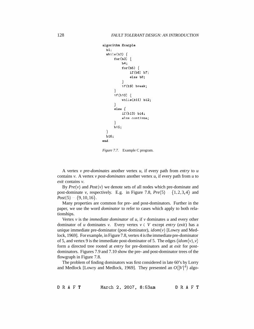
128 FAULT TOLERANT DESIGN: AN INTRODUCTION
�:�K�L�K�J���:�[�|�7ML���=��y:x� bHR�7� S yKx U � { ^ ûT=YK�fU �L� ^ û�=� RTLYK� U �J� ^ ûS�TfU �J� ^ �L� Rx=y7z:x �=� Rý S�TfU �J� ^ � � x:�K�fRý S�TfU � b�P ^ û�7� S y:x U � b:b ^ � b�{5Rýx7y7z:x ûS�TfU � b � ^ � b � Rx=y7zKx W:Y[Z=]�S�Z7� x5Rý� b � Rý� b � R�[�=�Figure 7.7. Example C program.
A vertex v pre-dominates another vertex u, if every path from entry to ucontains v. A vertex v post-dominates another vertex u, if every path from u toexit contains v.
By Pre % v & and Post % v & we denote sets of all nodes which pre-dominate andpost-dominate v, respectively. E.g. in Figure 7.8, Pre % 5 &ú*ðP 1 ( 2 ( 3 ( 4 S andPost % 5 &T*�P 9 ( 10 ( 16 S .
Many properties are common for pre- and post-dominators. Further in thepaper, we use the word dominator to refer to cases which apply to both rela-tionships.
Vertex v is the immediate dominator of u, if v dominates u and every otherdominator of u dominates v. Every vertex v � V except entry (exit) has aunique immediate pre-dominator (post-dominator), idom % v & [Lowry and Med-lock, 1969]. For example, in Figure 7.8, vertex 4 is the immediate pre-dominatorof 5, and vertex 9 is the immediate post-dominator of 5. The edges % idom % v &!( v &form a directed tree rooted at entry for pre-dominators and at exit for post-dominators. Figures 7.9 and 7.10 show the pre- and post-dominator trees of theflowgraph in Figure 7.8.
The problem of finding dominators was first considered in late 60’s by Lorryand Medlock [Lowry and Medlock, 1969]. They presented an O %h3V 3 4 & algo-
��������� � �����������������������! �"�$# ���������
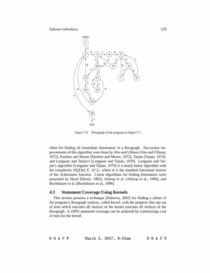
Software redundancy 129
1
2 3 4 5
69
7 8
10
1113
14 12
exit
entry
ab c d
j e
gf
i
q
t
l
ps
h
km
o
r
z
w
x
y
u
15
16
Figure 7.8. Flowgraph of the program in Figure 7.7.
rithm for finding all immediate dominators in a flowgraph. Successive im-provements of this algorithm were done by Aho and Ullman [Aho and Ullman,1972], Purdom and Moore [Purdom and Moore, 1972], Tarjan [Tarjan, 1974],and Lengauer and Tarjan’s [Lengauer and Tarjan, 1979]. Lengauer and Tar-jan’s algorithm [Lengauer and Tarjan, 1979] is a nearly-linear algorithm withthe complexity O %h3E 3α %h3E 3](!3V 3¾&R& , where α is the standard functional inverseof the Ackermann function. Linear algorithms for finding dominators werepresented by Harel [Harrel, 1985], Alstrup et al. [Alstrup et al., 1999], andBuchsbaum et al. [Buchsbaum et al., 1998].
4.3 Statement Coverage Using KernelsThis section presents a technique [Dubrova, 2005] for finding a subset of
the program’s flowgraph vertices, called kernel, with the property that any setof tests which executes all vertices of the kernel executes all vertices of theflowgraph. A 100% statement coverage can be achieved by constructing a setof tests for the kernel.
��������� � �����������������������! �"�$# ���������

130 FAULT TOLERANT DESIGN: AN INTRODUCTION
15
2
5
9
7
6
8
10
1
3
4
13
14
11
12
16
Figure 7.9. Pre-dominator tree of the flowgraph in Figure 7.8; shaded vertices are leaves of thetree in Figure 7.10.
¢¡~£ ¤¦¥�¤¦§s¤©¨�¥«ªo¬©A vertex v � V of the flowgraph is covered by a test case t
if the basic block of the program representing v is reached at least once duringthe execution of t.
The following Lemma is the basic property of the presented technique [Agrawal,1994].® ¡~¯°¯²±³
If a test case t covers u � V , then it covers any post-dominator of uas well: % t covers u &�´ % v � Post % u &R&Qµ % t covers v &!-Proof: If v post-dominates u, then every path from u to exit contains v. There-fore, if u is reached at least once during the execution of t, then v is reached,too. ¢¡~£ ¤¦¥�¤¦§s¤©¨�¥«ªo¬·¶
A kernel K of a flowgraph G is a subset of vertices of Gwhich satisfies the property that any set of tests which executes all vertices ofthe kernel executes all vertices of G. ¢¡~£ ¤¦¥�¤¦§s¤©¨�¥«ªo¬¹¸
Minimum kernel is a kernel of the smallest size.
Let Lpost (Lpre) denote the set of leaf vertices of the post-(pre-)dominator treeof G. The set LD
post º Lpost contains vertices of Lpost which pre-dominate some
��������� � �����������������������! �"�$# ���������
Software redundancy 131
vertex of Lpost :
LDpost *�P v 3$% v � Lpost &»´ % v � Pre % u & for some u � Lpost &`S�-
Similarly, the subset LDpre º Lpre contains all vertices of Lpre which post-dominate
some vertex of Lpre:
LDpre *�P v 37% v � Lpre &�´ % v � Post % u & for some u � Lpre &`S�-
Assume that the program execution terminates normally on all test casessupplied. Then the following statement holds.¼»½ ¡�¨¿¾A¡~¯Àªo¬Á
The set Lpost 2 LDpost is a minimum kernel.
Proof: Lemma 1 shows that, if a vertex of a flowgraph is covered by a testcase t, then all its post-dominators are also covered by t. Therefore, in order tocover all vertices of a flowgraph, it is sufficient to cover all leaves L post in itspost-dominator tree, i.e. Lpost is a kernel.
LDpost contains all vertices of Lpost which pre-dominate some vertex of Lpost .
If v is a pre-dominator of u, and u is covered by t, then v is also covered by t,since every path from entry to u contains v as well. Thus, any set of tests whichcovers Lpost 2 LD
post , covers Lpost as well. Since Lpost is a kernel, Lpost 2 LDpost
is a kernel, too.Next, we prove that the set Lpost 2 LD
post is a minimum kernel. Suppose thatthere exists another kernel, K � , such that 3K �¡3�³æ3 Lpost 2 LD
post 3 . If v � K � andv y� Lpost , then v � Post % u & for some u � Lpost . Since every path from u to exitcontains v, if u is reached at least once during the execution of some test case,then v is reached, too. Therefore, K � remains a kernel if we replace v by u.
Suppose we replaced all v � K � such that v y� Lpost by u � Lpost such thatv � Post % u & . Now, K �~� Lpost . If there exists w � Lpost 2 K � such that, for allu � K � , w y� Pre % u & then there exists at least one path from entry to each u whichdoes not contain w. This means that there exists a test set, formed by the setof paths path % u & where path % u & is the path to u which does not contain w, thatcovers K � but not w. According to Definition 7.2, this implies that K � is not akernel. Therefore, to guarantee that K � is a kernel, w must be a pre-dominatorof some u � K � , for all w � Lpost 2 K � . This implies that 3K �§3»*æ3 Lpost 2 LD
post 3 .The next theorem shows that the set Lpre 2 LD
pre is also a minimum kernel.¼»½ ¡�¨¿¾A¡~¯Àªo¬Â¶ 3 Lpost 2 LDpost 3 *æ3 Lpre 2 LD
pre 3]-The proof is done by showing that the proof of minimality of Theorem 7.1
can be carried out starting from Lpre.
��������� � �����������������������! �"�$# ���������

132 FAULT TOLERANT DESIGN: AN INTRODUCTION
2
15
11
12
1
14
5
6
3
7 84
9
10 13
16
Figure 7.10. Post-dominator tree of the flowgraph in Figure 7.8; shaded vertices are leaves ofthe tree in Figure 7.9.
4.4 Computing Minimum KernelsThis section presents an linear-time algorithm for computing minimum ker-
nels from [Dubrova, 2005]. The pseudo-code is shown in Figure 7.11.First, pre- and post-dominator trees of the flowgraph G *�% V ( E ( entry ( exit & ,
denoted by Tpre and Tpost , are computed. Then, the numbers of leaves ofthe trees, Lpre and Lpost , are compared. According to Theorems 7.1 and 7.2,both, Lpost 2 LD
post and Lpre 2 LDpre, represent minimum kernels. The procedureÃÅĦÆ@ÇÉÈËÊ
is applied to the smaller of the sets Lpre and Lpost .ÃÅĦÆ@ÇÉÈËÊchecks whether the leaves Lpre of the tree Tpre are dominated by
some vertex of Lpre in another tree, Tpost , or vice versa. In other words,ÃÅÄÁÆ@Ç¿ÈÌÊ
computes the set LDpre (LD
post ).¼»½ ¡�¨¿¾A¡~¯Àªo¬Í¸The algorithm ÎÐÏ~Ñ Æ Ï�Ò computes a minimum kernel of a flow-
graph G *�% V ( E ( entry ( exit & in O %h3V 3;5 3E 3¾& time.
Proof: The correctness of the algorithm follows directly from Theorems 7.1and 7.2. The complexity of the ÎÐÏ~Ñ Æ Ï�Ò is determined by the complexityof computing the Tpre and Tpost trees. A dominator tree can be computedin O %h3V 3h5 3E 3¾& time [Alstrup et al., 1999]. Thus, the overall complexity isO %h3V 3e5 3E 3¾& .
As an example, let us compute a minimum kernel for the flowgraph in Fig-ure 7.8. Its pre- and post-dominator trees are shown in Figures 7.9 and 7.10.Tpre has 7 leaves, Lpre *�P 7 ( 8 ( 9 ( 12 ( 14 ( 15 ( 16 S , and Tpost has 9 leaves, Lpost *��������� � �����������������������! �"�$# ���������
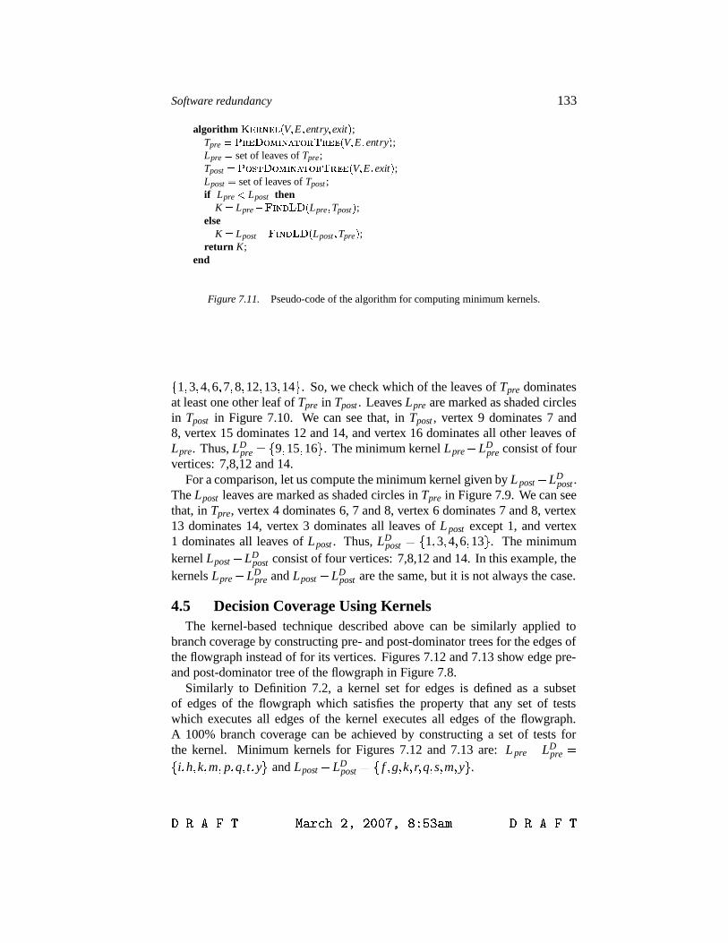
Software redundancy 133
algorithm ÓÅÔJÕkÖiÔ�×cK V ü E ü entry ü exit L ;Tpre M¢ØsÕkÔ�ÙËÚÜÛ�ÝÞÖkßJàHÚCÕiáÉÕkÔJÔNK V ü E ü entry L ;Lpre M set of leaves of Tpre;Tpost MâØsÚÜã�àkÙËÚÜÛ�ÝÞÖkßJàHÚCÕiáÉÕkÔJÔ7K V ü E ü exit L ;Lpost M set of leaves of Tpost ;if Lpre ä Lpost then
K M Lpre å3æ ÝÞÖiçCè~ÙöK Lpre ü Tpost L ;else
K M Lpost å3æ ÝéÖiçÜè�ÙöK Lpost ü Tpre L ;return K;
end
Figure 7.11. Pseudo-code of the algorithm for computing minimum kernels.
P 1 ( 3 ( 4 ( 6 ( 7 ( 8 ( 12 ( 13 ( 14 S . So, we check which of the leaves of Tpre dominatesat least one other leaf of Tpre in Tpost . Leaves Lpre are marked as shaded circlesin Tpost in Figure 7.10. We can see that, in Tpost , vertex 9 dominates 7 and8, vertex 15 dominates 12 and 14, and vertex 16 dominates all other leaves ofLpre. Thus, LD
pre *QP 9 ( 15 ( 16 S . The minimum kernel Lpre 2 LDpre consist of four
vertices: 7,8,12 and 14.For a comparison, let us compute the minimum kernel given by Lpost 2 LD
post .The Lpost leaves are marked as shaded circles in Tpre in Figure 7.9. We can seethat, in Tpre, vertex 4 dominates 6, 7 and 8, vertex 6 dominates 7 and 8, vertex13 dominates 14, vertex 3 dominates all leaves of Lpost except 1, and vertex1 dominates all leaves of Lpost . Thus, LD
post *jP 1 ( 3 ( 4 ( 6 ( 13 S . The minimumkernel Lpost 2 LD
post consist of four vertices: 7,8,12 and 14. In this example, thekernels Lpre 2 LD
pre and Lpost 2 LDpost are the same, but it is not always the case.
4.5 Decision Coverage Using KernelsThe kernel-based technique described above can be similarly applied to
branch coverage by constructing pre- and post-dominator trees for the edges ofthe flowgraph instead of for its vertices. Figures 7.12 and 7.13 show edge pre-and post-dominator tree of the flowgraph in Figure 7.8.
Similarly to Definition 7.2, a kernel set for edges is defined as a subsetof edges of the flowgraph which satisfies the property that any set of testswhich executes all edges of the kernel executes all edges of the flowgraph.A 100% branch coverage can be achieved by constructing a set of tests forthe kernel. Minimum kernels for Figures 7.12 and 7.13 are: Lpre 2 LD
pre *P i ( h ( k ( m ( p ( q ( t ( y S and Lpost 2 LDpost *�P f ( g ( k ( r( q ( s ( m ( y S .
��������� � �����������������������! �"�$# ���������

134 FAULT TOLERANT DESIGN: AN INTRODUCTION
d
y
i h
e
g f
z
j
u
a
b
w o
q s
t
l
p
x
c
r
km
Figure 7.12. Edge pre-dominator tree of the flowgraph in Figure 7.8; shaded vertices are leavesof the tree in Figure 7.13.
5. Problems7.1. A program consists of 10 independent routines, all of them being used
in the normal operation of the program. The probability that a routineis faulty is 0.10 for each of the routines. It is intended to use 3-versionprogramming, with voting to be conducted after execution of each routine.The effectiveness of the voting in eliminating faults is 0.85 when one of thethree routines is faulty and 0 when more than one routine is faulty. What isthe probability of a fault-free program:
(a) When only a single version is produced and no routine testing is con-ducted.
(b) When only a single version of each routine is used, but extensive routinetesting is conducted that reduces the fault content to 10% of the originallevel.
(c) When three-version programming is used.
��������� � �����������������������! �"�$# ���������

Software redundancy 135
z
b ay o
l
t
s
w
d
g cf
e
jq
x
k
u
p
r
m
ih
Figure 7.13. Edge post-dominator tree of the flowgraph in Figure 7.8; shaded vertices are leavesof the tree in Figure 7.12.
��������� � �����������������������! �"�$# ���������


Chapter 8
LEARNING FAULT-TOLERANCE FORM NATURE
1. Introduction
The gene regulatory network is one of the most important signaling net-works in living cells. It is composed from the interactions of proteins with thegenome. In this section, we consider a model of the gene regulatory network,called Kauffman network. Introduced by Kauffman in 1969 in the context ofgene expression and fitness landscapes [Kaufmann, 1969], Kauffman networkswere later applied to the problems of cell differentiation, immune response,evolution, and neural networks [Aldana et al., ]. They have also attracted theinterest of physicists due to their analogy with the disordered systems studiedin statistical mechanics, such as the mean field spin glass [Derrida and Pomeau,1986, Derrida and Flyvbjerg, 1986, Derrida and Flyvbjerg, 1987].
The Kauffman network is a class of random nk-Boolean networks. An nk-Boolean network is a synchronous Boolean automaton with n vertices. Eachvertex has exactly k incoming edges, assigned at random, and an associatedBoolean function. Functions are selected so that they evaluate to the values0 and 1 with given probabilities p and 1 2 p, respectively. Time is viewedas proceeding in discrete steps. At each step, the new state of a vertex v isa Boolean function of the previous states of the predecessors of v. Cellularautomata can be considered as a special case of random nk-Boolean networks,in which the incoming edges are assigned form the immediate neighbors.
The Kauffman network is an nk-Boolean network with the input fan-in two(k * 2) and the functions assigned independently an uniformly at random fromthe set of 22k * 16 possible Boolean functions (p * 0 - 5). The functions representthe rules of regulatory interactions between the genes. The states of verticesrepresent the status of gene expressions; "1" indicates that a gene is expressed,
��������� � �����������������������! �"�$# ���������

138 FAULT TOLERANT DESIGN: AN INTRODUCTION
"0" - not expressed. For edges, the value "1" means that a protein is present,"0" - absent.
The parameters k and p determine the dynamics of the network. If a vertexcontrols many other vertices and the number of controlled vertices grows intime, the network is said to be in a chaotic phase. Typically, such a behavioroccurs for large values of k, k ê n. The next states are random with respect to theprevious ones. The dynamics of the network is very sensitive to changes in thestate of a particular vertex, associated Boolean function, or network connection.
If a vertex controls only a small number of other vertices and their numberremains constant in time, a network is said to be in a frozen phase. Usually,independently on the initial state, after a few steps the network reaches a stablestate. This behavior typically occurs for small values of k, such as k * 0 or 1.
There is a critical line between the frozen and the chaotic phases, whenthe number of vertices controlled by a vertex grows in time, but only up to acertain limit. Statistical features of nk-Boolean networks on the critical line areshown to match the characteristics of real cells and organisms [Kaufmann, 1969,Kaufmann, 1993]. The minimal disturbances typically cause no variations inthe network’s dynamics. Only some rare events evoke a radical change.
For a given probability p, there is a critical number of inputs kc below whichthe network is in the frozen phase and above which the network is in the chaoticphase [Derrida and Pomeau, 1986]:
kc * 12p % 1 2 p & - (8.1)
For p * 0 - 5, the critical number of inputs is kc * 2, so the Kauffman networksare on the critical line.
Since the number of possible states of a Kauffman network is finite (up to2n), any sequence of consecutive states of a network eventually converges toeither a single state, or a cycle of states, called attractor. The number andlength of attractors represent two important parameters of the cell modeled bya Kauffman network. The number of attractors corresponds to the number ofdifferent cell types. For example, humans have n µ 25 - 000 genes and 254 celltypes. Attractor’s length corresponds to the cell cycle time. Cell cycle timerefers to the amount of time required for a cell to grow and divide into twodaughter cells. The length of the total cell cycle varies for different types ofcells.
Human body has a sophisticated system for maintaining normal cell repairand growth. The body interacts with cells through a feedback system thatsignals a cell to enter different phases of the cycle. If a person is sick, e.g has acancer, then this feedback system does not function normally and cancer cellsenter the cell cycle independently of the body’s signals. The number and lengthof attractors of a Kauffman network serve as indicators of the health of the
��������� � �����������������������! �"�$# ���������
Learning Fault-Tolerance from Nature 139
cell modeled by the network. Sensitivity of the attractors to different kind ofdisturbances, modeled by changing the state of a particular vertex, associatedBoolean function, or network connection, reflects the stability of the cell todamage, mutations and virus attacks.
Our interest in Kauffman networks is due to their attractive fault-tolerantfeatures. Kauffman networks exhibit a stable behavior, where different kind offaults, e.g. a change in the state of a particular vertex, or connection, typicallycause no variations in network’s dynamics. On the other hand, Kauffmannetworks have a potential for evolutionary improvements. If a sufficient numberof mutations is allowed, a network can adopt to the changing environment byre-configuring its structure. Another notable feature of Kauffman networksis that the subgraph induced by their relevant vertices usually consists of asingle connected component, rather than being scattered into groups of vertices.Determining which redundancy allocation scheme makes such a phenomenonpossible seems to be interesting problem.
2. Kauffman NetworksThe Kauffman Network is a directed cyclic graph G *�% V ( E & , where V is the
set of vertices and E � V � V is the set of edges connecting the vertices.The set V has n vertices. Each vertex v � V has exactly two incoming edges,
selected at random from V (including v itself). The set of predecessors of v isdenoted by Pv, Pv *�P u � V 36% u ( v &â� E S . The set of ancestors of v is denotedby Sv, Sv *�P u � V 37% v( u &â� E S .
Each vertex v � V has an associated Boolean function, fv, of type P 0 ( 1 S 2 ëP 0 ( 1 S . Functions are selected so that they evaluate to the values 0 and 1 withequal probability p * 0 - 5.
The state σv of a vertex v at time t 5 1 is determined by the states of itspredecessors u1 ( u2 � Pv as:
σv % t 5 1 &�* fv % σui % t &!( σu2 % t &R&!-The vector % σv1 % t &!( σv2 % t &!(R-R-R-`( σvn % t &R& represents the state of the network at timet. An example of a Kauffman network with ten vertices is shown in Figure 8.1.
An infinite sequence of consecutive states of a Kauffman network is calleda trajectory. A trajectory is uniquely defined by the initial state. Since thenumber of possible states is finite, all trajectories eventually converges to eithera single state, or a cycle of states, called attractor. The basin of attraction ofan attractor A is the set of all trajectories leading to A. The attractor length isthe number of states in the attractor’s cycle.
3. Redundant VerticesRedundancy is an essential feature of biological systems, insuring their cor-
rect behavior in presence of internal or external disturbances. An overwhelming
��������� � �����������������������! �"�$# ���������
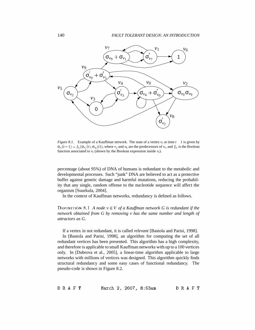
140 FAULT TOLERANT DESIGN: AN INTRODUCTION
0
1
v0
v6
v4
v3
σ ìv2
σ ìv7
σv4 í σ ìv0σ ìv3
σv2
v1
v9
v7
v2
σ ìv0 í σ ìv5
σv0 σv9
σv9 í σv1
v8
v5
Figure 8.1. Example of a Kauffman network. The state of a vertex vi at time t � 1 is given byσvi K t � 1 L¨M fvi K σv j K t L<ü σvk K t L£L , where v j and vk are the predecessors of vi, and fvi is the Booleanfunction associated to vi (shown by the Boolean expression inside vi).
percentage (about 95%) of DNA of humans is redundant to the metabolic anddevelopmental processes. Such “junk” DNA are believed to act as a protectivebuffer against genetic damage and harmful mutations, reducing the probabil-ity that any single, random offense to the nucleotide sequence will affect theorganism [Suurkula, 2004].
In the context of Kauffman networks, redundancy is defined as follows.
¢¡~£ ¤¦¥�¤¦§s¤©¨�¥Vîs¬©A node v � V of a Kauffman network G is redundant if the
network obtained from G by removing v has the same number and length ofattractors as G.
If a vertex in not redundant, it is called relevant [Bastola and Parisi, 1998].In [Bastola and Parisi, 1998], an algorithm for computing the set of all
redundant vertices has been presented. This algorithm has a high complexity,and therefore is applicable to small Kauffman networks with up to a 100 verticesonly. In [Dubrova et al., 2005], a linear-time algorithm applicable to largenetworks with millions of vertices was designed. This algorithm quickly findsstructural redundancy and some easy cases of functional redundancy. Thepseudo-code is shown in Figure 8.2.
��������� � �����������������������! �"�$# ���������

Learning Fault-Tolerance from Nature 141
algorithm ïðÔ�Û@Ú-ñCÔ�ïðÔJçÜòÜÖiçHßÜÖkàöK V ü E L/* I. Simplifying functions with one predecessor */for each v ó V do
if two incoming edges of v come from the same vertex thenSimplify fv;
/* II. Removing constants and implied */R1 M Ø;for each v ó V do
if fv is a constant thenAppend v at the end of R1;
for each v ó R1 dofor each u ó Sv å R1 do
Simplify fu by substituting constant fv;if fu is a constant then
Append u at the end of R1;Remove all v ó R1 and all edges connected to v;/* III. Simplifying 1-variable functions */for each v ó V do
if fv is a 1-variable function thenRemove the edge K u ü v L , where u is thepredecessor of v on which v does not depend;
/* IV. Removing functions with no output and implied */R2 M Ø;for each v ó V do
if Sv M Ø thenAppend v at the end of R2;
for each v ó R2 dofor each u ó Pv å R2 do
if all ancestors of u are in R2 thenAppend u at the end of R2;
Remove all v ó R2 and all edges connected to v;end
Figure 8.2. The algorithm for finding redundant vertices in Kauffman networks.
ô Ï~õ÷öùø¿Ï ô Ï Ç¿ú@Æ@Çsû�Æ@ü first checks whether there are vertices v with twoincoming edges coming from the same vertex. If yes, the associated functionsfv are simplified. In the example in Figure 8.1, there are not such cases ofredundancy.
Then,ô Ï~õ÷öùø¿Ï ô Ï Ç¿ú@Æ@Çsû�Æ@ü classifies as redundant all vertices v whose
associated function fv is constant 0 or constant 1. Such vertices are collectedin a list R1. Then, for every vertex v � R1, ancestors of v are visited and thefunctions associated to the ancestors are simplified. The simplification is doneby substituting the constant value of fv in the function of the ancestor u. Ifas a result of the simplification the function fu reduces to a constant, then u isappended to R1.
��������� � �����������������������! �"�$# ���������

142 FAULT TOLERANT DESIGN: AN INTRODUCTION
v5v2
v9
v7v1
σv2 σv9
σ ýv5
σ ýv7σv1 þ σv9
Figure 8.3. Reduced network GR for the Kauffman network in Figure 8.1.
In the example in Figure 8.1, vertices v3 and v6 have constant associatedfunctions. Thus, initially R1 *�P v3 ( v6 S . The vertex v3 has an ancestor v4. The
01000
10111
11000
01010
00101 10101
00111
11010
11110
00110
00000
10001 00001
00010
10110
11100
10011
10000
01011
00100
01110
11111
10111
11011
11101 01101
0100101111
01100
00011
10010
10100
Figure 8.4. State transition graph of the Kauffman network in Figure 8.3. Each vertex representsa 5-tuple K σ K v1 L σ K v2 L σ K v5 L σ K v7 L σ K v9 L£L of values of states on the relevant vertices.
��������� � �����������������������! �"�$# ���������
Learning Fault-Tolerance from Nature 143
Boolean function associated to v4 is a single-variable function which dependsonly on its predecessor v3. By substituting σv3 by fv3 * 0 in the Booleanexpression of v4, we get fv4 * 0 � * 1. Since fv4 reduces to a constant, it isappended to R1.
The vertex v6 has no ancestors, so no simplification is done. The vertex v4
has ancestors v0 and v3. The vertex v3 is already a constant. By substituting σv4
by fv4 * 1 in the Boolean function associated to v0, we get fv0 * 1 5 σ �v0* 1.
The vertex v0 is appended to R1.Similarly, the associated functions of the ancestors v2 and v9 of v0 are sim-
plified to fv2 * 1 4 σv9 * σv9 and fv9 * 1 �I5 σ �v5* σ �v5
. The ancestor v8 remainsunchanged because is does not depend on v0. Since no new vertices are ap-pended to R1, the phase I ends. The vertices R1 *�P v0 ( v3 ( v4 ( v6 S and all edgesconnected to these vertices are removed from the network.
Second,ô Ï~õ÷öùø¿Ï ô Ï Ç¿ú@Æ@Çsû�Æ�ü finds all vertices whose associated function
fv is a single-variable function. The edge between v and the predecessor of von which v does not depend is removed.
In the example in Figure 8.1, vertices v1, v2, v5, v8 and v9 have single-variable associated functions. Recall, that after simplifications in the phase II,fv2 * σv9 and fv9 * σ �v5
and the function of v4 is a constant. The edges from thepredecessors of v1, v2, v5, v8 on which they do not depend are removed.
Next,ô Ï~õ÷öùø¿Ï ô Ï Ç¿ú@Æ@Çsû�Æ@ü classifies as redundant all vertices which have
no ancestors. Such vertices are collected in a list R2. For every vertex v � R2,both predecessors of v are visited. If all ancestors of some predecessor u � Pv
are redundant, u is appended at the end of R2.In the example in Figure 8.1, the vertex v8 has no ancestors, thus R2 * P v8 S .
None of other vertices has a predecessor with all ancestors redundant. So, novertex are added to R2 at phase IV. The vertex v8 is removed from the network.
The worst-case time complexity ofô Ï�õ°öùøÉÏ ô Ï Ç�ú@Æ@Çsû¿Æ@ü is O %h3V 3e5 3E 3¾& ,
where 3V 3 is the number of vertices and 3E 3 is the number of edges in G.As we mentioned before,
ô Ï~õ÷öùø¿Ï ô Ï Ç¿ú@Æ@Çsû�Æ�ü might not identify all casesof functional redundancy. For example, a vertex may have a constant outputvalue due to the correlation of its input variables. For example, if a vertex v withan associated OR (AND) function has predecessors u1 and u2 with functionsfu1 * σw and fu2 * σ �w, then the value of fv is always 1 (0). Such cases ofredundancy are not detected by
ô Ï~õ÷öùø¿Ï ô Ï Ç�ú�Æ@Çsû�Æ@ü .Let GR be the reduced network obtained from G by removing redundant
vertices. The reduced network for the example in Figure 8.1 is shown in Fig-ure 8.3. Its state transition graph is given in Figure 8.4. Each vertex of thestate transition graph represents a 5-tuple % σ % v1 & σ % v2 & σ % v5 & σ % v7 & σ % v9 &R& of val-ues of states on the relevant vertices v1, v2, v5, v7, v9. There is two attractors:P 01111 ( 01110 ( 00100 ( 10000 ( 10011 ( 01011 S , of length six, and P 00101 ( 11010 ( 00111 ( 01010 S ,of length four. By Definition 8.1, by removing redundant vertices we do not
��������� � �����������������������! �"�$# ���������

144 FAULT TOLERANT DESIGN: AN INTRODUCTION
change the total number and length of attractors in a Kauffman network. There-fore, G has the same number and length of attractors as GR.
4. Connected ComponentsVertices of GR induce a number of connected components. ¢¡~£ ¤¦¥�¤¦§s¤©¨�¥Vîs¬·¶
Two vertices are in the same connected component if andonly if there is an undirected path between them.
A path is called undirected if it ignores the direction of edges. For example,the network in Figure 8.3 has two components: P v2 ( v5 ( v9 S and P v1 ( v7 S .
Finding connected components can be done in O %h3V 3x5¸3E 3¾& time, where 3V 3 isthe number of vertices and 3E 3 is the number of edges of GR, using the followingalgorithm [Tarjan, 1972]. To find a connected component number i, the functionÿ ö�õ���ö Æ Ï Æ@ü�� Ï û Ñ����1% v & is called for a vertex v which has not been assigned toa component yet.
ÿ ö¿õ��oö Æ Ï Æ@ü�� Ï û Ñ���� does nothing if v has been assignedto a component already. Otherwise,
ÿ ö¿õ��oö Æ Ï Æ@ü�� Ï û Ñ���� assigns v to thecomponent i and calls itself recursively for all children and parents of v. Theprocess repeats with the counter i incremented until all vertices are assigned.
5. Computing attractors by compositionThis section shows that it is possible to compute attractors of a network G
compositionally from the attractors of the connected components of the reducednetwork GR [Dubrova and Teslenko, 2005].
Let GA be a connected component of GR and AA be an attractor of GA. Anattractor AA of length L is represented by a sequence of states Σ0 ( Σ1 (R-R-R-h( ΣL A 1 ,where Σ . i � 1 � modL is the next state of the state Σi, i ��P 0 ( 1 (R-R-R-I( L 2 1 S .
The support set of an attractor AA, sup % AA & , is the set of vertices of GA. Forexample, the left-hand side connected component in Figure 8.3 has the supportset P v2 ( v5 ( v9 S . ¢¡~£ ¤¦¥�¤¦§s¤©¨�¥Vîs¬¹¸
Given two attractors AA *� ΣA0 ( ΣA
1 (R-R-R-`( ΣALA and AB *� ΣB
0 ( ΣB1 (R-R-R-h( ΣB
LB ,such that sup % AA & � sup % AB &+* Ø, the composition of AA and AB is a set of at-tractors defined by:
AA � AB * d A 1�k 9 0
P Ak Swhere d is the greatest common divisor of LA and LB, each attractor Ak is oflength m, m is the least common multiple of LA and LB, and the ith state of Ak
is a concatenation of % i mod LA & th state of AA and %R% i 5 k & mod LB & th state ofAB:
Σki * ΣA
i mod LAΣB. i � k � mod LB
��������� � �����������������������! �"�$# ���������

Learning Fault-Tolerance from Nature 145
for k �WP 0 ( 1 (R-R-R-I( d 2 1 S , i � P 0 ( 1 (R-R-R-`( m 2 1 S and "mod" is the operation divisionmodulo.
As an example, consider two attractors AA *� ΣA0 ( ΣA
1 and AB *� ΣB0 ( ΣB
1 ( ΣB2 .
We have d * 1 and m * 6, so AA � AB * P A0 S , where the states Σ0i , i �P 0 ( 1 (R-R-R-I( 5 S are defined by
Σ00 * ΣA
0 ΣB0 Σ0
3 * ΣA1 ΣB
0
Σ01 * ΣA
1 ΣB1 Σ0
4 * ΣA0 ΣB
1
Σ02 * ΣA
0 ΣB2 Σ0
5 * ΣA1 ΣB
2 -The composition of attractors is extended to the composition of sets of at-
tractors as follows. ¢¡~£ ¤¦¥�¤¦§s¤©¨�¥Vîs¬��Given two sets of attractors P A11 ( A12 (R-R-R-h( A1L1 S and P A21 (
A22 (R-R-R-h( A2L2 S , such that sup % A1i &�� sup % A2 j &ú* Ø, for all i � P 1 ( 2 (R-R-R-I( L1 S ,j � P 1 ( 2 (R-R-R-`( L2 S , the composition of sets is defined by:P A11 ( A12 (R-R-R-h( A1L1 S � P A21 ( A22 (R-R-R-h( A2L2 S�*�
� . i1 � i2 � z�� 1 � � � ��� L1 ��� � 1 � � � ��� L2 �A1i1 � A2i2
where “ � ” is the Cartesian product.® ¡~¯°¯²± ¶The composition AA � AB consists of all possible cyclic sequences
of states which can be obtained from AA and AB.
Proof: By Definition 8.3, the result of the composition of AA and AB is dattractors P A0 ( A1 (R-R-R-h( Ad A 1 S of length m each, where d is the greatest commondivisor of LA and LB is m and the least common multiple of LA and LB.
Consider any two states of the attractor Ak, Σki and Σk
j , for some i ( j �P 0 ( 1 (R-R-R-I( m 2 1 S , i y* j, and some k � P 0 ( 1 (R-R-R-!( d 2 1 S . By Definition 8.3,
Σki * ΣA
i mod LAΣB. i � k � mod LB
andΣk
j * ΣAj mod LA
ΣB. j � k � mod LB-
We prove that % ΣAi mod LA
* ΣAj mod LA
&Oµ% ΣB. i � k � mod LBy* ΣB. j � k � mod LB
&!-If ΣA
i mod LA* ΣB
j mod LB, then we can express j as
j * i 5 X 4 LA ( (8.2)
��������� � �����������������������! �"�$# ���������

146 FAULT TOLERANT DESIGN: AN INTRODUCTION
where X is some constant which satisfies X 4 LA ³ m.By substituting j by (8.2) in the expression % j 5 k & mod LB, we get% j 5 k & mod LB *�% i 5 X 4 LA 5 k & mod LB - (8.3)
Clearly, if X 4 LA is not evenly divisible by LB, then the right-hand side ofthe expression (8.3) is not equal to % i 5 k & mod LB. On the other hand, X 4 LA
cannot be evenly divisible by LB, because LA y* LB and X 4 LA ³ m. Thus% i 5 X 4 LA 5 k & mod LB y*�% i 5 k & mod LB
and therefore the states ΣB. j � k � mod LBand ΣB. i � k � mod LB
are different. Similarly,we can show that% ΣB. i � k � mod LB
* ΣB. j � k � mod LB&`µ% ΣA
i mod LAy* ΣA
j mod LA&!-
Therefore, for a given k ��P 0 ( 1 (R-R-R-I( d 2 1 S , no two states in the attractor Ak areequal.
Similarly to the above, we can show that no two states in two differentattractors can be the same. If the first parts of two states are the same, than thesecond parts differ due to the property% k 5 X 4 LA & mod LB y* 0
for any k � P 0 ( 1 (R-R-R-I( d 2 1 S .There are LA 4 LB different pairs of indexes in the Cartesian product P 1 (R-R-R-`(
LA S�� P 1 (R-R-R-`( LB S . Thus, since LA 4 LB * m 4 d, at least d attractors of lengthm are necessary to represent all possible combinations. Since no two states ofA0 ( A1 (R-R-R-h( Ad A 1 are the same, exactly d attractors of length m are sufficient torepresent all possible combinations.
Let P G1 ( G2 (R-R-R-`( Gp S be the set of components of GR. Throughout the restof the section, we use Ni to denote the number of attractors of Gi, Ai j to de-note jth attractor Gi, and Li j to denote the length of Ai j, i * P 1 ( 2 (R-R-R-I( p S ,j *�P 1 ( 2 (R-R-R-!( Ni S .
Let I * I1 � I2 � -R-R-c� Ip be the Cartesian product of sets Ii * P i1 ( i2 (R-R-R-h( iNi S ,where p is the number of components of GR. The set Ii represents indexes ofattractors of the component Gi. For example, if Ni * 3, then Gi has 3 attractors:Ai1 ( Ai2 and Ai3. The set Ii is then Ii *sP 1 ( 2 ( 3 S . The set I enumerates allpossible elements of the sets Ii. For example, if p * 2, N1 * 2 and N2 * 3, thenI *�P7% 1 ( 1 &!(`% 1 ( 2 &!(�% 1 ( 3 &!(`% 2 ( 1 &!(`% 2 ( 2 &!(`% 2 ( 3 &`S�-��������� � �����������������������! �"�$# ���������

Learning Fault-Tolerance from Nature 147¼»½ ¡�¨¿¾A¡~¯ îs¬ÁThe set of attractors A of the reduced network GR with p
components can be computed as
A * �� . i1 � � � ��� ip � z I
%R% A1i1 � A2i2 & � P A3i3 SF&7-R-R- � P Apip SProof: (1) The state space of any component is partitioned into basins ofattraction. There are no common states between different basins of attraction.Thus, different attractors of the same component have no common states.
(2) Since in any pair of components % Gi ( G j & , i ( j *�P 1 ( 2 (R-R-R-I( p S , i y* j, Gi
and G j do not have vertices in common, the support sets of attractors of Gi andG j do not intersect. Thus, different attractors of different components have nocommon states.
(3) The set I enumerates all possible combinators of p-tuple of indexes ofattractors of components. By definition of the Cartesian product, every p-tupleof I differ at least in one position.
(4) From (1), (2) and (3) we can conclude that the set of attractors obtainedby the composition %R% A1i1 � A2i2 & � P A3i3 SF&7-R-R- � P Apip S for a given % i1 (R-R-R-h( ip &T� I,differs from the set of attractors obtained for any other p-tuple % i �1 (R-R-R-h( i �p &1� I.
(5) From Lemma 2, we know that the composition A1i1 � A2i2 representsall possible cyclic sequences of states which can be obtained from A1i1 andA2i2 . We can iteratively apply Lemma 2 to the result of A1i1 � A2i2 composedwith A3i3 , etc., to show that the composition %R% A1i1 � A2i2 & � P A3i3 SF&7-R-R- � P Apip Srepresents all possible attractors which can be obtained from p attractors A ji1 ,j *�P 1 ( 2 (R-R-R-!( p S .
(6) From (4) and (5) we can conclude that the union of compositions overall p-tuples of I represents the attractors of GR.
The following results follow directly from the Theorem 8.1.® ¡~¯°¯²± ¸The total number of attractors in the reduced network GR with p
components is given by
N * ∑� . i1 � � � � � ip � z I
p
∏j 9 2
%R%R% L1i1 � L2i2 & � L3i3 &7-R-R- � L j A 1i j � 1 & � L ji j
where "� " is the least common multiple operation and " � " is the greatest commondivisor operation.® ¡~¯°¯²±��
The maximum length of attractors in the reduced network GR isgiven by
Lmax * max� . i1 � � � � � ip � z I%R% L1i1 � L2i2 & � L3i3 &7-R-R- � Lpip
where "� " is the least common multiple operation.
��������� � �����������������������! �"�$# ���������

148 FAULT TOLERANT DESIGN: AN INTRODUCTION
v5v2
v9
σv2 σv9
σ !v5v7
σv1 σ !v7
v1
Figure 8.5. Example of a reduced network GR with two components.
000
10 01
00
11
001
101
111
110
010A12
(a) (b)
A11
100
011
A21
Figure 8.6. (a) State space of the component G1 M û v2 ü v5 ü v9 ý . There are two attractors,A11 M#" 011 ü 100 $ and A12 M#" 000 ü 001 ü 101 ü 111 ü 110 ü 010 $ . (b) State space of the componentG2 MWû v1 ü v7 ý . There is one attractor, A21 M%" 00 ü 10 ü 11 ü 01 $ .
By Definition 8.1, by removing redundant vertices we do not change the totalnumber and the maximum length of attractors of an RBN. Therefore, N andLmax given by Lemmas 3 and 4 are the same for the original network G.
As an example, consider the network in Figure 8.5 with two components:G1 *QP v2 ( v5 ( v9 S and G2 *QP v1 ( v7 S . Their state spaces are shown in Figure 8.6.The first component has two attractors: A11 *& 011 ( 100 of length L11 * 2 andA12 *' 000 ( 001 ( 101 ( 111 ( 110 ( 010 of length L12 * 6. The second componenthas one attractor A21 *( 00 ( 10 ( 11 ( 01 of length L21 * 4.
The Cartesian product of I1 *sP 1 ( 2 S and I2 *sP 1 S contains 2 pairs: I *P7% 1 ( 1 &!(`% 2 ( 1 &`S . For the pair % 1 ( 1 & we have L11 � L21 * 2 � 4 * 2 and L11 � L21 *2 � 4 * 4. So, A11 and A21 compose into two attractors of length 4:
A11 � A21 * P 01100 ( 10010 ( 01111 ( 10001 ( 01110 ( 10011 ( 01101 ( 10000 S�-
The order of vertices in the states is v2 ( v5 ( v9 ( v1 ( v7.
��������� � �����������������������! �"�$# ���������

Learning Fault-Tolerance from Nature 149
B C G D n ½ � ÇCGDn
E 4:� Ï
E 4:�*) + Á )
Figure 8.7. Crossed dots show the average number of vertices in GR as a function of the numberof vertices n in G. Average results for 10000 networks.
Similarly, for the pair % 2 ( 1 & we have L12 � L21 * 6 � 4 * 2 and L12 � L21 *6 � 4 * 12. So, A12 and A21 compose into two attractors of length 12:
A12 � A21 * P 00000 ( 00110 ( 10111 ( 11101 ( 11000 ( 01010 (00011 ( 00101 ( 10100 ( 11110 ( 11011 ( 01001 ( 00010 ( 00111 ( 10101 ( 11100 ( 11010 ( 01011 (
00001 ( 00100 ( 10110 ( 11111 ( 11001 ( 01000 S$-The total number of attractors is N * 4. The maximum attractor length is
Lmax * 12.
6. Simulation ResultsThis section shows simulation results for Kauffman networks of sizes from
10 to 107 vertices. Figure 8.7 plots the average number of relevant verticescomputed using
ô Ï~õ÷öùø¿Ï ô Ï Ç¿ú@Æ@Çsû�Æ�ü as a function of n. Table 8.1 presentsthe same results numerically in columns 1 and 2. The number of relevantvertices scales as , n.
Column 4 gives the average number of connected components in GR as afunction of n. The number of components grows of order of logn.
Column 3 of Table 8.1 shows the number of vertices in the largest componentof GR. As we can see, the size of this component is Θ % n & . “Giant” componentphenomena is well-studied in general random graphs [Molloy and Reed, 1998].For a random graph with n vertices in which each edge appears independentlywith probability p * c 8 n, c ¹ 1, the size of the largest component of the graphis known to be Θ % n & . No theoretical explanation why the giant componentphenomena appears in the the subgraph induced by the relevant vertices ofKauffman networks has been found yet.
��������� � �����������������������! �"�$# ���������

150 FAULT TOLERANT DESIGN: AN INTRODUCTION
size of number ofthe largest components-
G- -
GR-
component of GR in GR
10 5 5 1102 25 25 1103 93 92 1104 270 266 2105 690 682 3106 1614 1596 3107 3502 3463 4
Table 8.1. Average results for 10000 networks.
6.1 Fault-tolerance issuesKauffman networks have two attractive features: stability and evolvability.
Extensive experimental results confirm that Kauffman networks are tolerant tofaults, i.e. typically the number and length of attractors does not change whena fault occurs [Kaufmann, 1993, Aldana et al., ]. The following types of faultmodels are used by biologists to model mutations in the cell, damage from theenvironment, or disease attacks, in Kauffman networks:
a predecessor of a vertex v is changed, i.e. the edge % u ( v & is replaced by anedge % w( v & , v( u ( w � V ;
the state of a vertex is changed to the complemented value;
Boolean function of a vertex is changed to a different Boolean function.
On one hand, the stability of Kauffman networks is due to the large percentageof redundancy in the network: ê�% n 2., n & of n vertices are typically redundant.On the other hand, the stability is due to the non-uniqueness of the networkrepresentation: the same dynamic behavior (state space transition graph) canbe achieved by many different Kauffman networks.
An essential feature of living organisms is their capability to adopt to achanging environment. Kauffman networks have been shown to be successfulin evolving to a predefined target function, confirming their purpose of beingmodels of living cells.
��������� � �����������������������! �"�$# ���������

References
[Agrawal, 1994] Agrawal, H. (1994). Dominators, super blocks, and program coverage. InSymposium on principles of programming languages, pages 25–34, Portland, Oregon.
[Agrawal, 1999] Agrawal, H. (1999). Efficient coverage testing using global dominator graphs.In Workshop on Program Analysis for Software Tools and Engineering, pages 11–20,Toulouse, France.
[Aho and Ullman, 1972] Aho, A. V. and Ullman, J. D. (1972). The Theory of Parsing, Trans-lating, and Compiling, Vol. II. Prentice-Hall, Englewood Cliffs, NJ.
[Aldana et al., ] Aldana, M., Coopersmith, S., and Kadanoff, L. P. Boolean dynamics withrandom couplings. http://arXiv.org/ abs/adap-org/9305001.
[Alstrup et al., 1999] Alstrup, S., Harel, D., Lauridsen, P. W., and Thorup, M. (1999). Domi-nators in linear time. SIAM Journal on Computing, 28(6):2117–2132.
[Ball, 1993] Ball, T. (1993). What’s in a region?: or computing control dependence regions innear-linear time for reducible control flow. ACM Letters on Programming Languages andSystems (LOPLAS), 2:1–16.
[Bastola and Parisi, 1998] Bastola, U. and Parisi, G. (1998). The modular structure of Kauffmannetworks. Phys. D, 115:219.
[Beizer, 1990] Beizer, B. (1990). Software Testing Techniques. Van Nostrand Reinhold, NewYork.
[Bertolino and Marre, 1994] Bertolino, A. and Marre, M. (1994). Automatic generation ofpath covers based on the control flow analysis of computer programs. IEEE Transactions onSoftware Engineering, 20:885 – 899.
[Buchsbaum et al., 1998] Buchsbaum, A. L., Kaplan, H., Rogers, A., and Westbrook, J. R.(1998). A new, simpler linear-time dominators algorithm. ACM Transactions on Program-ming Languages and Systems, 20(6):1265–1296.
[Derrida and Flyvbjerg, 1986] Derrida, B. and Flyvbjerg, H. (1986). Multivalley structure inKaufmann’s model: Analogy with spin glass. J. Phys. A: Math. Gen., 19:L1103.
��������� � �����������������������! �"�$# ���������

152 FAULT TOLERANT DESIGN: AN INTRODUCTION
[Derrida and Flyvbjerg, 1987] Derrida, B. and Flyvbjerg, H. (1987). Distribution of local mag-netizations in random networks of automata. J. Phys. A: Math. Gen., 20:L1107.
[Derrida and Pomeau, 1986] Derrida, B. and Pomeau, Y. (1986). Random networks of au-tomata: a simple annealed approximation. Biophys. Lett., 1:45.
[Dubrova, 2005] Dubrova, E. (2005). Structural testing based on minimum kernels. In Pro-ceedings of DATE’2005, Munich, Germany.
[Dubrova and Teslenko, 2005] Dubrova, E. and Teslenko, M. (2005). Compositional propertiesof random boolean networks. Physics Review Letters.
[Dubrova et al., 2005] Dubrova, E., Teslenko, M., and Tenhunen, H. (2005). Computing attrac-tors in dynamic networks. In Proceedings of International Symposium on Applied Computing(IADIS’2005), pages 535–543, Algarve, Portugal.
[Harrel, 1985] Harrel, D. (1985). A linear time algorithm for finding dominators in flow graphsand related problems. Annual Symposium on Theory of Computing, 17(1):185–194.
[Kaufmann, 1969] Kaufmann, S. A. (1969). Metabolic stability and epigenesis in randomlyconstructed nets. Journal of Theoretical Biology, 22:437–467.
[Kaufmann, 1993] Kaufmann, S. A. (1993). The Origins of Order: Self-Organization andSelection of Evolution. Oxford University Press, Oxford.
[Lengauer and Tarjan, 1979] Lengauer, T. and Tarjan, R. E. (1979). A fast algorithm for findingdominators in a flowgraph. Transactions of Programming Languages and Systems, 1(1):121–141.
[Lowry and Medlock, 1969] Lowry, E. S. and Medlock, C. W. (1969). Object code optimization.Communications of the ACM, 12(1):13–22.
[Molloy and Reed, 1998] Molloy, M. and Reed, B. (1998). The size of the giant component ofa random graph with a given degree sequence. Combin. Probab. Comput., 7:295–305.
[Ntafos, 1988] Ntafos, S. (1988). A comparison of some structural testing strategies. IEEETransactions on Software Engineering, 14(6):868–874.
[Podgurski, 1991] Podgurski, A. (1991). Forward control dependence, chain equivalence, andtheir preservation by reordering transformations. Technical Report CES-91- 18, ComputerEngineering & Science Department, Case Western Reserve University, Cleveland, Ohio,USA.
[Purdom and Moore, 1972] Purdom, P. W. and Moore, E. F. (1972). Immediate predominatorsin a directed graph. Communications of the ACM, 15(8):777–778.
[Roper, 1994] Roper, M. (1994). Software Testing. McGraw-Hill Book Company, London.
[Suurkula, 2004] Suurkula, J. (2004). Over 95 percent of DNA has largely unknown function.http://www.psrast.org/junkdna.htm.
[Tarjan, 1972] Tarjan, R. E. (1972). Depth-first search and linear graph algorithms. SIAMJournal on Computing, 1(2):146–160.
��������� � �����������������������! �"�$# ���������

REFERENCES 153
[Tarjan, 1974] Tarjan, R. E. (1974). Finding dominators in a directed graphs. Journal ofComputing, 3(1):62–89.
[Watson, 1996] Watson, A. H. (1996). Structured testing: Analysis and extensions. TechnicalReport TR-528-96, Princeton University.
��������� � �����������������������! �"�$# ���������