fault mapping with the refraction microtremor and seismic

$: Fault Mapping with the Refraction Microtremor and Seismic$
FAULT MAPPING WITH THE REFRACTION MICROTREMOR AND SEISMIC

REFRACTION METHODS ALONG THE LOS OSOS FAULT ZONE

A Thesis

Presented to the Faculty of

California Polytechnic State University

San Luis Obispo

In Partial Satisfaction

Of the Requirements for the Degree of

Master of Science in Civil and Environmental Engineering

By

Justin Riley Martos

November 2012

ii

© 2012

Justin Riley Martos

ALL RIGHTS RESERVED

iii

COMMITTEE MEMBERSHIP

TITLE: Fault Mapping with the Refraction Microtremor and

Seismic Refraction Methods along the Los Osos Fault

Zone

AUTHOR: Justin Riley Martos

DATE SUBMITTED: November 2012

Committee Chair: Robb Moss, Associate Professor

Committee Member: Gregg Fiegel, Professor

Committee Member: John Jasbinsek, Assistant Professor

iv

ABSTRACT

Fault Mapping with the Refraction Microtremor and Seismic Refraction Methods

along the Los Osos Fault Zone

By Justin Riley Martos

The presence of active fault traces in proximity to any new infrastructure project is a

major concern for the design process. The relative displacements that can be

experienced in surface fault rupture during a seismic event must be either entirely

avoided or mitigated in some way. Blind faults present a significant challenge to

engineers attempting to identify these hazards. Current standards of practice employed

to locate these features are time consuming and costly. This work investigates the

geophysical methods of refraction microtremor (ReMi) and seismic refraction with regard

to their applicability in this task. By imaging a distinct lateral variation in the shear wave

velocity (Vs) profile across a short horizontal distance, these methods may provide a

means of constraining traditional investigation techniques to a more focused area. The

ReMi method is still very new, but holds key advantages over other geophysical

methods in its ease of application and ability to achieve good results in highly urban

settings. It is one of the few geophysical techniques that does not suffer in the presence

of high amplitude ambient vibrations. The seismic refraction method is here applied in

an attempt to corroborate data obtained through the ReMi analysis procedure.

Sensitivity, precision parametric studies are carried out in order to learn how to best

apply the ReMi method. Both tests are then applied at a previously trenched fault trace

to determine whether the data can be matched to the subsurface information. Finally,

the methods are deployed at a location with an inferred fault trace where little to nothing

is known about the subsurface. The precision study indicates a coefficient of variation

v

for the ReMi method on the order of 7%. At the known fault trace both methods

generally agree qualitatively with available subsurface data and each other. Using the

ReMi method, a marked shift is observed in the Vs profile laterally across the fault trace.

In the case of the inferred fault trace, the same type of lateral variation in the Vs profile is

observed using the ReMi method. The seismic refraction at this site does not agree with

the ReMi data, but seems reasonable given the visible geomorphology. Receiver arrays

placed in close proximity to the inferred fault trace recorded erratic signals during

seismic refraction testing, and displayed abnormal response modes after transforming

the ReMi data to frequency-slowness space. These anomalies may possibly be

attributed to the presence of abnormal subsurface structural geometry indicative of

faulting.

vi

ACKNOWLEDGEMENTS

This work would not have been possible without the help I received from the many

people involved with this project. First and foremost among them is my advisor, Prof.

Robb Moss. His guidance throughout this endeavor was essential to its success from

start to finish. I greatly appreciate the patience and encouragement he provided during

my struggles. The help and direction provided me a framework that aided the steady

progress toward my goal, while also allowing me the space to draw my own conclusions

along the way.

I would like to express my deep gratitude to Professors Gregg Fiegel and John

Jasbinsek for taking the time to review my work and provide insightful suggestions of

ways to improve upon it. I only provided them with one week to read this entire paper

because of my rush to complete the degree requirement, but they both adjusted their

schedules to accommodate my needs. I consider this a personal favor and am in their

debt.

Jason Auyeung and Dr. Moss both contributed a significant amount of their own time to

help me with the data collection process in the field. I cannot thank them enough for the

many hours we spent together in the hot sun placing arrays and swinging sledge

hammers. Without their help my job would have been beyond exhausting.

This work involved learning the use of a lot of software I had no previous experience

using. Satish Pullammanappallil of Optim Software provided me with continual support

in using the Optim programs for data processing and analysis. Throughout this project

he supplied invaluable help with troubleshooting, general procedural guidelines, and

vii

interpretive insight. I am very thankful for his patient aid with many questions I’m sure

seemed very novice to someone with his experience.

Thomas Blake of Fugro Consultants, Inc. also deserves a sincere thank you for his

suggestions on how to better collect and analyze seismic refraction data. Tom had no

obligation to help me, but he immediately dedicated time to answer my many questions,

and even processed some of the data himself with software unavailable to me.

During my research it was at times necessary to turn to more experienced geophysicists

for explanations of subtle theory and terminology usage. It was very helpful to be able to

turn to Prof. Brady Cox and his doctoral student Clinton Wood in these instances. They

always took the time to fully answer any questions and to ensure that I understood the

explanations. I enjoyed the time I was able to spend with them collecting geophysical

data for a National Science Foundation project at the San Francisco Trans-bay Transit

Center construction site.

I extend a special thanks to John Madonna and Diane Sawyer of San Luis Obispo

County for their contributions to my work. Without their help this project would have

been impossible. I greatly appreciate their patience and cooperation throughout this

work.

Finally I must thank my family and friends, especially my mother and father, who have

been there for me through good times and bad. Their emotional support was essential

to get me through to the end. It was the laughter and relaxation their company provided

during my small breaks from this work that enabled me to keep returning to it. I would

have never reached the finish line without some occasional time to unwind.

viii

Table of Contents

LIST OF TABLES ......................................................................................................... xiii

LIST OF FIGURES ....................................................................................................... xiv

Chapter 1: Statement of Research ................................................................................. 1

1.1: Introduction .......................................................................................................... 1

1.2: Fault Rupture and Blind Fault Mapping ................................................................ 2

1.3: Project Scope ....................................................................................................... 3

1.4: Organization of Thesis ......................................................................................... 4

Chapter 2: Review of Methods to Obtain a Site Shear Wave Velocity Profile.................. 5

2.1: Introduction to Vs logging ..................................................................................... 5

2.2: Direct Measurement Methods .............................................................................. 6

2.2.1: Downhole Logging ......................................................................................... 6

2.2.2: Crosshole Logging ......................................................................................... 9

2.2.3: Suspension PS-Logging ...............................................................................11

2.2.4: Seismic Cone Penetration Test (SCPT) ........................................................13

2.3: Body Wave Methods ...........................................................................................14

2.3.1: Seismic Refraction ........................................................................................14

2.3.2: Seismic Reflection ........................................................................................21

2.4: Surface Wave Methods .......................................................................................23

2.4.1: Steady-State Method ....................................................................................24

2.4.2: Spectral Analysis of Surface Waves (SASW)................................................26

2.4.3: Microtremor Analysis ....................................................................................28

2.4.4: Multichannel Analysis of Surface Waves (MASW) ........................................31

2.4.5: Refraction Microtremor (ReMi) ......................................................................34

2.4.5.1: Theory ....................................................................................................34

2.4.5.2: Comparisons with other methods ...........................................................37

ix

2.5: Intra-method Variability .......................................................................................39

2.5.1: Variability within the ReMi Method ................................................................39

2.5.2: Intra-method Variability of Other Tests .........................................................40

Chapter 3: Testing Methods ..........................................................................................42

3.1: Refraction Microtremor ........................................................................................42

3.1.1: Field Setup ...................................................................................................42

3.1.2: Data Collection and Exportation with VScope ...............................................45

3.1.3: Data Processing and Analysis ......................................................................49

3.1.3.1: Processing Data and Making Dispersion Curve Picks in

ReMiVspect v4.0 .................................................................................................50

3.1.3.2: Forward Modeling of a 1D Profile in ReMiDisper v4.0 ............................55

3.1.3.3: Assembling a 2D Cross-Section in ReMiDisper v4.0 ..............................58

3.2: Seismic Refraction ..............................................................................................59

3.2.1: Field Setup ...................................................................................................60

3.2.2: Data Collection with VibraScope ...................................................................61

3.2.3: Data Processing and Analysis ......................................................................63

3.2.3.1: Interpretation of Seismograms and Making First Brake Point (FBP)

Picks in VScope ..................................................................................................64

3.2.3.2: Exporting for Processing through SeisOpt@2D v5.0 ..............................66

3.2.3.3: Creating a 2D P-Wave Velocity Profile Using SeisOpt@2D v5.0 ............67

Chapter 4: Site Locations and Array Placement ............................................................73

4.1: Crops Field C-31 .................................................................................................74

4.2: Ingley Site ...........................................................................................................76

4.2.1: Existing Information ......................................................................................76

4.2.1.1: Trenching at Ingley Site T-2 ...................................................................78

4.2.1.2: Geomorphology .....................................................................................81

4.2.2: Array Placement ...........................................................................................81

x

4.3: Frontera Site .......................................................................................................83

4.3.1: Geomorphology ............................................................................................83

4.3.2: Array Placement ...........................................................................................83

Chapter 5: Crops Field C-31 Data Analysis ...................................................................85

5.1: Refraction Microtremor ........................................................................................86

5.1.1: Highland Road Arrays ...................................................................................86

5.1.1.1: Highland Road Precision Study ..............................................................88

5.1.1.2: Highland Road Parametric Study ...........................................................93

5.1.2: Stenner Creek Arrays ...................................................................................98

5.1.3: Quality and Uncertainty of Measurements ....................................................99

5.2: Seismic Refraction ............................................................................................ 103

5.2.1: Quality and Uncertainty of Measurements .................................................. 104

5.2.2: Theoretical Travel Times ............................................................................ 105

5.3: Inter-Method Comparisons ................................................................................ 107

5.4: Summary of Findings ........................................................................................ 108

Chapter 6: Ingley Site Data Analysis ........................................................................... 110

6.1: Refraction Microtremor ...................................................................................... 111

6.1.1: Lower Arrays NE of Ingley Trench T-2 ........................................................ 112

6.1.1.1: Individual p-f Spectral Ratio Plots and Picks ........................................ 112

6.1.1.2: Forward Modeling and Combined 2D Profiles ...................................... 119

6.1.2: Upper Arrays on Scarp Expression near Ingley Trench T-2 ........................ 121

6.1.2.1: Array I-4 Slope Sensitivity Study .......................................................... 121

6.1.2.2: Multiple Trend Effects in Arrays I-5 and I-6........................................... 124

6.1.2.3: Forward Modeling and Combined 2D Profile ........................................ 130

6.1.3: Comparison of Hanging and Footwall Profiles ............................................ 131


6.2.1: Array Setup and Data Collection ................................................................. 132

xi

6.2.2: First Break Point Picking ............................................................................. 133

6.2.3: Model Profiles ............................................................................................. 134

6.3: Comparison of Results ...................................................................................... 138


Chapter 7: Frontera Site Data Analysis ........................................................................ 142

7.1: Refraction Microtremor ...................................................................................... 143

7.1.1: Ambient Recording Artifacts ....................................................................... 144

7.1.2: Comparison of Filtered and Non-Filtered Drift ............................................. 146

7.1.3: Comparison of M-2a and M-2b ................................................................... 149

7.1.4: Comparison of Arrays M-1 and M-2 ............................................................ 151

7.1.5: Signal Source Comparison ......................................................................... 153

7.1.5.1: Active Source Comparison ................................................................... 153

7.1.5.2: Off-Line Actively Induced Signal Measurements .................................. 156

7.1.5.3: Differences Observed between In-Line Active Energy Produced

Off of Opposite Array Ends ............................................................................... 159

7.1.5.4: Irregular Spectral Power Distributions .................................................. 160

7.1.6: Forward Modeling and 2D Profile Assemblies............................................. 163


7.2.1: Array Setup and Data Collection ................................................................. 166

7.2.2: First Break Picking ...................................................................................... 167

7.2.3: Model Profiles ............................................................................................. 170

7.2.3.1: M-5 Models .......................................................................................... 171

7.2.3.2: M-6 Models .......................................................................................... 173

7.2.3.3: M-7 Models and Demonstration of Modeling Uncertainty ..................... 175


Chapter 8: Conclusions and Recommendations .......................................................... 183

8.1: Summary .......................................................................................................... 183

xii

8.2: Research Findings ............................................................................................ 184

8.3: Improvements on Testing Methods ................................................................... 187

8.4: Opportunities for Further Investigation .............................................................. 188

References .................................................................................................................. 190

xiii

LIST OF TABLES

TABLE 2.1: APPLICABILITY OF ANALYSIS METHODS (FROM TOKIMATSU ET AL. 1992) ...........29

TABLE 2.2: ANGULAR COVERAGE OF SLOWNESS INTERVALS (FROM LOUIE 2001) ...............36

TABLE 2.3: INTRA-METHOD VARIABILITY ANALYZING ARRAY ORIENTATION AND SIGNAL

SOURCE INFLUENCES (FROM COX & BEEKMAN 2011).................................................39

TABLE 4.1: TESTING SCHEDULE FOR CROPS FIELD C-31 ARRAYS ......................................75

TABLE 4.2: SENSOR ARRAY DETAILS AND TESTING SCHEDULE FOR THE INGLEY SITE ..........82

TABLE 4.3: TABLE 4.2: SENSOR ARRAY DETAILS AND TESTING SCHEDULE FOR THE

FRONTERA SITE .......................................................................................................84

TABLE 5.1: SUMMARY OF FINDINGS OF PRECISION STUDY ON HIGHLAND ROAD ..................90

TABLE 5.2: LAYER DEPTH AND VELOCITY STATISTICS FOR PRECISION STUDY ON HIGHLAND

ROAD ......................................................................................................................90

xiv

LIST OF FIGURES

FIGURE 2.1: SCHEMATIC OF DOWNHOLE VS LOGGING SETUP (FROM ASTM D7400-08) ....... 8

FIGURE 2.2: EXAMPLE OF DOWNHOLE SEISMOGRAM SHOWING FIRST ARRIVALS

OF P AND S-WAVES (FROM ASTM D7400-08) ............................................................ 9

FIGURE 2.3: SCHEMATIC OF CROSSHOLE VS LOGGING (FROM ASTM D4428M-07) .............11

FIGURE 2.4: SCHEMATIC OF UP-HOLE SUSPENSION LOGGING SETUP (FROM GEOVISION

GEOPHYSICAL SYSTEMS) .........................................................................................12

FIGURE 2.5: SCHEMATIC OF SCPT VS LOGGING (FROM ASTM D7400-08) .........................14

2.6: SCHEMATIC OF SEISMIC REFRACTION ARRAY SETUP (FROM ASTM D5777) ................15

FIGURE 2.7: WAVE REFRACTION AND THE CRITICAL ANGLE OF INCIDENCE

(FROM REDPATH 1973) ............................................................................................16

FIGURE 2.8: SCHEMATIC SHOWING FIRST ARRIVALS FROM DIRECT AND REFRACTED

WAVES WITH A CORRESPONDING DISTANCE-TIME PLOT (FROM REDPATH 1973) .........17

FIGURE 2.9: WAVES REFRACTING ALONG DIPPING BEDS AND THE CORRESPONDING

DISTANCE TIME PLOT (FROM REDPATH 1973) ............................................................18

FIGURE 2.10: DEFINITION OF DELAY TIMES (FROM REDPATH 1973) ...................................20

FIGURE 2.11: SCHEMATIC OF SEISMIC REFLECTION SURVEY (ILLINOIS STATE GEOLOGIC

SURVEY) .................................................................................................................22

FIGURE 2.12: SCHEMATIC OF RAYLEIGH WAVE PROPAGATION AND PARTICLE MOTION ........24

FIGURE 2.13: SCHEMATIC OF STEADY STATE METHOD ARRAY AND WAVE FIELD

(FROM YUAN 2011) ..................................................................................................25

FIGURE 2.14: RAYLEIGH WAVE PARTICLE MOTION AT VARYING DEPTHS AS A FUNCTION

OF WAVELENGTH (FROM YUAN 2011) ........................................................................26

FIGURE 2.15: SCHEMATIC OF SASW ARRAY (FROM YUAN 2011) .......................................27

FIGURE 2.16: EXAMPLE OF COMPOSITE EXPERIMENTAL DISPERSION CURVE WITH

THEORETICAL DISPERSION CURVE FIT (FROM YUAN 2011) .........................................28

FIGURE 2.17: SUGGESTED SENSOR ARRAY FOR MICROTREMOR ANALYSIS

(FROM TOKIMATSU ET AL. 1992) ................................................................................30

FIGURE 2.18: EXAMPLE OF F-K SPECTRA AT SELECTED FREQUENCIES

(FROM TOKIMATSU ET AL. 1992) ................................................................................31

FIGURE 2.19: SCHEMATIC OF MASW ARRAY (FROM YUAN 2011) ......................................32

FIGURE 2.20: EXAMPLE OF EXPANDED FREQUENCY RANGE OF DATA FROM COMBINED

PASSIVE AND ACTIVE RECORDS (FROM YUAN 2011) ..................................................33

xv

FIGURE 2.21: EXAMPLE SLOWNESS-FREQUENCY PLOT DEPICTING DISPERSION PICKS

AND ZONE OF F-K ALIASING (FROM LOUIE 2001) ........................................................35

FIGURE 2.22: PLOT OF INTER-METHOD AT PARKWAY, WELLINGTON, NEW ZEALAND

(FROM LOUIE 2001) ..................................................................................................37

FIGURE 2.23: (A) PLACEMENT ON A RAILWAY EMBANKMENT OF SASW AND REMI

ARRAYS WITH SUSPENSION PS-LOGGED HOLE SHOWN AT S-1 AND (B) CROSS

SECTION OF EMBANKMENT SOIL PROFILE (FROM PÉREZ-SANTISTEBAN ET AL. 2011) ...38

FIGURE 2.24: PLOT ILLUSTRATING COMPARISON BETWEEN METHODS ON A RAILWAY

EMBANKMENT (FROM PÉREZ-SANTISTEBAN ET AL. 2011)............................................38

FIGURE 2.25: PLOT ILLUSTRATING COMPARISONS OF ARRAY ORIENTATION AND SIGNAL

SOURCE TYPE (FROM COX & BEEKMAN 2011) ...........................................................40

FIGURE 3.1: DAQ SETUP MENU .......................................................................................45

FIGURE 3.2: DATA ACQUISITION CONFIGURATION SETTINGS WINDOW ................................46

FIGURE 3.3: VSCOPE HOME WINDOW SHOWING “START” BUTTON, RECORDING STATUS

BAR, AND AN EXAMPLE ABNORMAL TRACE RECORD ...................................................47

FIGURE 3.4: LOCAL DATABASE OF RECORDINGS FROM THE CURRENT PROJECT .................49

FIGURE 3.5: REMIVSPECT V4.0 DATA READING PARAMETERS ...........................................50

FIGURE 3.6: GRAPHICALLY REPRESENTED DATA WITH CORRECT NUMBER OF POINTS ........51

FIGURE 3.7: P-F TRANSFORMATION INPUT PARAMETERS ...................................................52

FIGURE 3.8: SEISOPT JPEG OUTPUT FILE AFTER MAKING PICKS ON A COMBINED

P-F PLOT .................................................................................................................54

FIGURE 3.9: MODEL PROFILE PRIOR TO DISPERSION CURVE FITTING SHOWING

EXPERIMENTAL PICKS VS. THEORETICAL DISPERSION CURVE .....................................55

FIGURE 3.10: AUTOMATIC DISPERSION INVERSION TOOL PARAMETERS WINDOW ................57

FIGURE 3.11: EXAMPLE OF A 2D CROSS SECTION ASSEMBLED FROM MULTIPLE 1D

REMI PROFILES .......................................................................................................59

FIGURE 3.12: AUTO OPERATION SETTINGS FOR AUTOMATED SEISMIC REFRACTION

DATA COLLECTION ...................................................................................................62

FIGURE 3.13: VIEW OF VSCOPE PICKER MODULE SHOWING SCALE OPTIONS, PICKS

TABLE AND EXAMPLE FIRST BREAK POINT PICKS .......................................................65

FIGURE 3.14: VELOCITY MODEL VIEWING WINDOW ..........................................................68

FIGURE 3.15: RIOTS SETTINGS WINDOW .........................................................................68

FIGURE 4.1: VICINITY MAP DEPICTING INGLEY, AND CROPS FIELD C-31 SITES ....................73

xvi

FIGURE 4.2: SITE PLAN OF CROPS FIELD C-31 DEPICTING ARRAY LOCATIONS AS LINE

SEGMENTS ..............................................................................................................75

FIGURE 4.3: DETAILED GEOLOGIC MAP SHOWING INVESTIGATION LOCATIONS AS

WELL AS OBSERVED AND INFERRED FAULT TRACES (FROM LETTIS AND HALL, 1994) ....77

FIGURE 4.4: DIAGRAMMATIC LOG OF INGLEY TRENCH T-2 SHOWING OLDER ALLUVIUM

THRUST OVER YOUNGER (FROM LETTIS AND HALL, 1994) ..........................................79

FIGURE 4.5: POSSIBLE INTERPRETATIONS OF THE OVERALL FAULT BEHAVIOR BASED

UPON TRENCH LOGS AND GEOMORPHIC EXPRESSION (FROM LETTIS AND

HALL, 1994) ............................................................................................................80

FIGURE 4.6: PLAN OF THE INGLEY SITE SHOWING SENSOR ARRAY PLACEMENT IN

PROXIMITY TO THE 6M SCARP AND TRENCH T-2 DISCUSSED IN LETTIS AND

HALL (1994) ............................................................................................................82

FIGURE 4.7: PLAN OF THE FRONTERA SITE ARRAYS WITH AN INSET OF A RECENT

SATELLITE OVERLAY DEPICTING THE GEOMORPHIC EXPRESSION IDENTIFIED IN

THE FIELD IN THE SHADED AREA ...............................................................................84

FIGURE 5.1: SITE PLAN OF CROPS FIELD C-31 DEPICTING ARRAY LOCATIONS AS LINE

SEGMENTS ..............................................................................................................85

FIGURE 5.2: SIESOPT P-F SPECTRAL RATIO PLOTS FOR CF-1 SHOWING (A) SUITE 1, (B)

SUITE 2 AND (C) SUITE 3 ...........................................................................................87

FIGURE 5.3: VS30 PROFILE ILLUSTRATING VARIANCE WITHIN THE REMI METHOD WHILE

HOLDING ARRAY LOCATION AND ORIENTATION CONSTANT .........................................89

FIGURE 5.4: PICKS FROM ALL PRECISION STUDY TRIALS PLOTTED SIMULTANEOUSLY IN

FREQUENCY-PHASE VELOCITY SPACE ......................................................................91

FIGURE 5.5: PICKS FROM ALL PRECISION STUDY TRIALS PLOTTED SIMULTANEOUSLY IN

WAVELENGTH-PHASE VELOCITY SPACE ....................................................................91

FIGURE 5.6: THEORETICAL DISPERSION CURVE FITS FROM AUTOMATIC INVERSION FOR

(A) TRIAL ONE, (B) TRIAL TWO AND (C) TRIAL THREE IN PERIOD-VELOCITY SPACE .......92

FIGURE 5.7: CF-2 P-F PLOT OF COMBINED PASSIVE SIGNAL RECORDS ..............................94

FIGURE 5.8: CF-2 RECORDING WITH HAMMER BLOWS ON A STEEL PLATE OFF-END

OF THE ARRAY .........................................................................................................95

FIGURE 5.9: CF-2 RECORDING WITH HAMMER BLOWS AND NO PLATE OFF-END OF THE

ARRAY ....................................................................................................................96

FIGURE 5.10: CF-2 RECORDINGS WITH HAMMER BLOWS AT (A) 5M AND (B) 15M

OFFSETS FROM THE ARRAY LINE PERPENDICULAR TO THE MIDPOINT ..........................97

xvii

FIGURE 5.11: DIAGRAM OF WAVE-FRONT PROPAGATION FROM SOURCES OFFSET

PERPENDICULAR TO THE RECEIVER ARRAY ...............................................................98

FIGURE 5.12: CF-4 P-F SPECTRAL PLOT WITH PICKS ........................................................99

FIGURE 5.13: CF-2 RECORDING WITH HAMMER BLOWS ON A STEEL PLATE OFF-END

OF THE ARRAY SYMMETRICALLY OPPOSITE TO THE DATA SHOWN IN FIGURE 5.7 ....... 100

FIGURE 5.14: PLOT OF AMPLITUDE RECORDINGS FOR ARRAY CF-2 INDICATING

INTERFERENCE IN CHANNELS 11 AND 12 ................................................................. 102

FIGURE 5.15: SEISMOGRAMS OF ARRAY CF-2 SHOWING INTERFERENCE NOISE OF A

POSSIBLE UTILITY LINE ALONG HIGHLAND ROAD ...................................................... 102

FIGURE 5.16: FREQUENCY SPECTRUM PLOT OF CHANNELS 1,2,11 AND 12 FOR ARRAY

CF-2 SHOWING DIFFERENCES IN HIGH FREQUENCY AMPLITUDES ............................. 103

FIGURE 5.17: RECEIVER AND SOURCE COORDINATE DIAGRAMS FOR (A) CF-1,

(B) CF-2 AND CF-4 ................................................................................................ 104

FIGURE 5.18: EXPERIMENTAL SEISMIC REFRACTION SEISMOGRAMS OBTAINED WITH

SOURCE 8M OFF-END OF CF-2 ............................................................................... 105

FIGURE 5.19: THEORETICAL SEISMIC REFRACTION SEISMOGRAMS FOR THE AREA

ADJACENT TO CF-2 ................................................................................................ 106

FIGURE 5.20: COMPARISONS BETWEEN SCPT DATA AND REMI PROFILES MODELED

BOTH BLINDLY AND IN AN ATTEMPT TO MATCH SCPT DATA AT (A) HIGHLAND

ROAD AND (B) STENNER CREEK .............................................................................. 108

FIGURE 6.1: PLAN OF THE INGLEY SITE SHOWING SENSOR ARRAY PLACEMENT IN

PROXIMITY TO THE 6M SCARP AND TRENCH T-2 DISCUSSED IN LETTIS AND

HALL (1994) .......................................................................................................... 111

FIGURE 6.2: P-F SPECTRAL RATIO PLOT OF AMBIENT SIGNAL RECORD FOR I-1 ................. 113

FIGURE 6.3: P-F SPECTRAL RATIO PLOT OF UNINTENTIONAL MID-ARRAY VIBRATIONS

RECORD FOR I-1 .................................................................................................... 114

FIGURE 6.4: SEISMOGRAPHS OF UNINTENTIONAL MID-ARRAY VIBRATIONS RECORD

FOR I-1 .................................................................................................................. 114

FIGURE 6.5: P-F SPECTRAL RATIO PLOT WITH PICKS FOR WALKING RECORD OF I-1 .......... 115

FIGURE 6.6: SEISMOGRAPHS OF A WALKING RECORD FOR I-1 .......................................... 115

FIGURE 6.7: P-F SPECTRAL RATIO PLOT WITH PICKS FOR COMBINED ACTIVE AND

PASSIVE RECORDS OF I-1 ....................................................................................... 116

FIGURE 6.8: SCATTER OF PICKS FROM THE ACTIVE AND COMBINED

ACTIVE/PASSIVE P-F PLOTS .................................................................................... 116

xviii

FIGURE 6.9: P-F SPECTRAL RATIO PLOT WITH PICKS FOR I-2 ........................................... 118

FIGURE 6.10: P-F SPECTRAL RATIO PLOT WITH PICKS FOR I-3 ......................................... 118

FIGURE 6.11: ASSEMBLED 2D PROFILE WITH BOTTOM LAYER VS = 600M/S ....................... 119

FIGURE 6.12: ASSEMBLED 2D PROFILE WITH BOTTOM LAYER VS = 700M/S AND FIT TO

INFERRED GEOLOGY IN LETTIS AND HALL (1994) ..................................................... 120

FIGURE 6.13: MODEL PROFILE FOR I-1 FIT WITH BOTTOM LAYER VS = 700M/S .................. 121

FIGURE 6.14: ARRAY ELEVATION PROFILE FOR I-4 (NO HORIZONTAL EXAGGERATION) ...... 122

FIGURE 6.15: SPECTRAL RATIO P-F PLOT OF I-4 DATA A) WITH CORRECTED RECEIVER

COORDINATES ....................................................................................................... 123

FIGURE 6.16: SCATTER PLOT OF PICKS FROM SLOPE CORRECTED AND

NON-CORRECTED P-F PLOTS .................................................................................. 124

FIGURE 6.17: SPECTRAL RATIO P-F PLOT OF (A) UPPER TREND AND (B) LOWER

TREND PICKS ON PASSIVE RECORDS FOR ARRAY I-5 ............................................... 125

FIGURE 6.18: SPECTRAL RATIO P-F PLOT FOR ACTIVE RECORD WITH PICKS FOR

HAMMER AND PLATE BLOWS AT ARRAY I-5 .............................................................. 126

FIGURE 6.19: SCATTER PLOT COMPARING UPPER AND LOWER TREND DISPERSION

PICKS TO ACTIVE PICKS ......................................................................................... 126

FIGURE 6.20: SPECTRAL RATIO P-F PLOT SHOWING A TYPICAL PASSIVE RECORDING

AT I-6 .................................................................................................................... 128

FIGURE 6.21: SPECTRAL RATIO P-F PLOT SHOWING STACKED PASSIVE RECORDINGS

AND PICKS AT I-6 ................................................................................................... 128

FIGURE 6.22: SPECTRAL RATIO P-F PLOT SHOWING STACKED ACTIVE RECORDS AND

PICKS AT I-6 .......................................................................................................... 129

FIGURE 6.23: SCATTER PLOT OF ACTIVE AND PASSIVE RECORD PICKS FOR ARRAY I-6 ..... 129

FIGURE 6.24: ASSEMBLED 2D MODEL PROFILE FOR UPPER INGLEY ARRAYS .................... 131

FIGURE 6.25: I-6 MODEL VS PROFILE .............................................................................. 131

FIGURE 6.26: OVERALL ASSEMBLED 2D MODEL PROFILE OF INGLEY REMI ARRAYS

WITH A ZONE OF UNCERTAINTY BETWEEN HANGING AND FOOTWALLS ....................... 132

FIGURE 6.27: DIAGRAM OF ARRAY I-7 ............................................................................ 133

FIGURE 6.28: OFF-END SHOT GATHER WITH FIRST BREAK POINT PICKS AT ARRAY I-7 ..... 134

FIGURE 6.29: SEISOPT .................................................................................................. 135

FIGURE 6.30: SEISOPT .................................................................................................. 135

FIGURE 6.31: SEISOPT@2D TOMOGRAPHY MODEL FOR ARRAY I-7 IN (A) MAXIMUM

COLOR DISPLAY AND (B) 5 COLOR DISPLAY ............................................................... 136

xix

FIGURE 6.32: TWO-LAYER MODEL PROFILE OF I-7 FROM IXREFRAX (T. BLAKE,

PERSONAL COMMUNICATION, SEPTEMBER 11, 2012) ................................................ 137

FIGURE 6.33: SUMMARY OF MODEL FIGURES AND PAST TRENCHING FOR INGLEY SITE

(TRENCH DATA FROM LETTIS AND HALL (1994)) ....................................................... 140

FIGURE 7.1: PLAN OF THE FRONTERA SITE ARRAYS WITH AN INSET OF A RECENT

SATELLITE OVERLAY DEPICTING THE GEOMORPHIC EXPRESSION IDENTIFIED

IN THE FIELD IN THE SHADED AREA ......................................................................... 143

FIGURE 7.2: EXAMPLE P-F PLOT OF AMBIENT RECORDINGS TAKEN AT FRONTERA SITE

ARRAY M-3 ............................................................................................................ 144

FIGURE 7.3: SEISMOGRAPHS OF AMBIENT SIGNAL RECORDED AT ARRAY M-3 (A) WITH

SIGNAL DRIFT AND (B) CORRECTED FOR SIGNAL DRIFT WITH THE APPLICATION

OF A LOW CUT FILTER AT 1HZ................................................................................. 147

FIGURE 7.4: P-F SPECTRA RATIO PLOT OF DATA PROCESSED (A) WITHOUT DRIFT

CORRECTION AND (B) WITH DRIFT CORRECTION ...................................................... 148

FIGURE 7.5: P-F SPECTRAL RATIO PLOTS FOR (A) 8M SPACING AND (B) 4M SPACING

AT ARRAY M-2 ....................................................................................................... 150

FIGURE 7.6: DISPERSION PICKS FROM 8 AND 4M SPACED ARRAYS AT M-2 SHOWING

FOURTH ORDER POLYNOMIAL FITS TO THE FULL DATA SET AND UPPER AND

LOWER BOUNDS .................................................................................................... 151

FIGURE 7.7: P-F SPECTRAL RATIO PLOT INCLUDING DISPERSION PICKS FOR

ARRAY M-1 ............................................................................................................ 152

FIGURE 7.8: COMPARISON BETWEEN ARRAY M-1 DISPERSION PICKS AND THE

CURVE FIT TO BOTH SETS OF DISPERSION PICKS AT ARRAY M-2 .............................. 152

FIGURE 7.9: P-F SPECTRAL RATIO PLOTS OF WALKING INDUCED SIGNAL AT ARRAY M-3

WITH DISPERSION PICKS ALONG THE (A) UPPER TREND AND (B) LOWER TREND ......... 154

FIGURE 7.10: P-F SPECTRAL RATIO PLOTS OF OFF-END HAMMER BLOW ENERGY AT

ARRAY M-3 WITH DISPERSION PICKS ALONG THE (A) UPPER TREND AND

(B) LOWER TREND .................................................................................................. 155

FIGURE 7.11: SCATTER PLOT OF DISPERSION PICKS FOR UPPER AND LOWER TRENDS

WITH HAMMER AND WALKING ENERGY AT ARRAY M-3 .............................................. 156

FIGURE 7.12: P-F SPECTRAL RATIO PLOT OF HAMMER ENERGY ORIGINATING AT A

LOCATION PERPENDICULARLY OFFSET FROM THE MIDPOINT OF ARRAY (A) M-3

AND (B) M-4 ........................................................................................................... 158

xx

FIGURE 7.13: P-F SPECTRAL RATIO PLOTS FOR ARRAY M-5 CONTAINING OFF-END

HAMMER ENERGY FROM (A) THE SE AND (B) THE NW .............................................. 160

FIGURE 7.14: P-F SPECTRA RATIO PLOTS WITH HAMMER BLOWS OFF-END OF THE

(A) NORTH AND (B) SOUTH SIDE OF ARRAY M-6 ....................................................... 162

FIGURE 7.15: P-F SPECTRA RATIO PLOTS WITH HAMMER BLOWS OFF-END OF THE

(A) SOUTH AND (B) NORTH SIDES OF ARRAY M-6 ..................................................... 163

FIGURE 7.16: 1D MODEL PROFILE FOR ARRAY M-2 ......................................................... 164




FIGURE 7.20: ASSEMBLED 2D REMI PROFILE FOR THE FRONTERA SITE ........................... 166

FIGURE 7.21: DIAGRAM OF FRONTERA SEISMIC REFRACTION ARRAYS ............................. 167

FIGURE 7.22: SEISMIC REFRACTION RECORD FOR ARRAY M-5 WITH SOURCE

LOCATED BETWEEN RECEIVERS 4 AND 5 ................................................................. 168


LOCATED 8M OFF-END OF RECEIVER 1 ................................................................... 169





FIGURE 7.26: 2D TOMOGRAPHY OF ARRAY M-5 DATA WITH (A) 257 COLORS AND

(B) 3 COLORS ........................................................................................................ 171

FIGURE 7.27: LAYER MODEL OF ARRAY M-5 DATA OUTPUT FROM IXREFRAX ................... 172


FIGURE 7.29: 2D TOMOGRAPHY OF ARRAY M-6 DATA WITH (A) 257 COLORS AND

(B) 3 COLORS ........................................................................................................ 174

FIGURE 7.30: LAYER MODEL OF ARRAY M-6 DATA OUTPUT FROM IXREFRAX

(T. BLAKE, PERSONAL COMMUNICATION, SEPTEMBER 11, 2012) ............................... 175

FIGURE 7.31: 2D TOMOGRAPHY MODEL OUTPUT FROM SEISOPT FOR ARRAY M-7

WITH (A) 257 COLORS AND (B) 5 COLORS ................................................................ 176





xxi

FIGURE 7.34: LAYER MODEL OF ARRAY M-7 DATA OUTPUT FROM IXREFRAX

(T. BLAKE, PERSONAL COMMUNICATION, SEPTEMBER 11, 2012) .............................. 179


1

Chapter 1: Statement of Research

1.1: Introduction

In recent decades the advances in the field of applied geophysics have provided

engineers with a new tool to aid in shallow subsurface investigations. Theory originally

developed to help determine the Earth’s deep layer structure is now employed widely in

the near surface for a variety of purposes. These methods have been successfully used

for a number of engineering applications, a few among them include locating petroleum

reserves, determining water table depths for well water drilling, and developing soil

stiffness profiles to aid in characterizing site response during seismic events.

There are a number of different methods available that involve the measurement

of either body or surface waves. These methods are discussed in detail in chapter 2.

The field of applied geophysics is expanding rapidly as more and more scientists and

engineers have begun to explore its potential. Within just the last 20 years a number of

new techniques have surfaced that provide different means of applying the same

underlying principals of wave propagation. As is always the case, new methods warrant

significant amounts of research into their applicability. Many questions remain

unanswered with regards to the circumstances where these methods provide accurate

and/or precise results.

Some of the geophysical techniques available to engineers have significant

advantage over other investigation methods in the areas of cost, and time. It is for this

reason that many private companies in addition to academic institutions now apply these

techniques to corroborate traditional investigation results. In many cases, a field team

as small as two persons can collect all the necessary data at a small site in a full day’s

2

work. With some methods, such as the refraction microtremor (ReMi) and seismic

refraction techniques, achieving adequate results requires no more equipment than what

will fit in a small gardening wagon.

This body of work investigates the potential of the two methods mentioned in the

previous paragraph as fault mapping tools. Should these techniques prove efficient and

effective, engineers would have available a much cheaper and faster means of locating

fault traces.

1.2: Fault Rupture and Blind Fault Mapping

During seismic events it is not uncommon for the relative displacement between

structural blocks to propagate to the ground surface. This can result in offsetting

horizontally, vertically, or a combination of the two depending upon the fault regime. Any

structures that rest atop a fault trace that suddenly displaces in this nature could sustain

significant damage depending on the degree of offsetting. No man-made structure can

resist such forces, but some have been designed with enough ductility to allow for some

degree of displacement. Where possible, building on sites with active faults should

always be avoided.

After the 1971 San Fernando earthquake in California, the state legislature

passed the Alquist-Priolo Act in an attempt to reduce future damages from surface fault

rupture. This act prohibits building new structures for human occupancy within mapped

zones containing known active fault traces (R. Moss, personal communication, April 13,

2011). Although this law helps reduce the risk of damage from surface fault rupture,

many active faults exist that remain unmapped.

3

Many known active fault traces exhibit some surface expression and are easily

identifiable to trained geologists. Unfortunately, it is not uncommon for them to be blind

in nature (show no surface expression). Blind faults exist where the feature has been

covered by newer material that has not yet experienced rupture. Under small

displacements this material may behave in a ductile manner rather than exhibiting a

brittle rupture, and the trace will remain masked.

Locating these blind fault traces can be very expensive and time consuming with

traditional drilling or trenching techniques. These methods provide highly localized

information when the area being searched is often quite expansive. The application of

geophysical methods could potentially become a much more cost and time effective tool

to aid in narrowing down the possible trace location.

1.3: Project Scope

The primary goal of this thesis project is to investigate the possible application of

the refraction microtremor and seismic refraction methods as tools for fault mapping. In

order to reach this goal it was necessary to carry out a number of studies within the

refraction microtremor method to learn how to best apply the technique. These included

parametric studies to determine the effects of array geometry, relative source location,

and signal type, as well as a precision study to characterize the uncertainty involved in

the measurement process.

After determining best practices for each technique, this work attempts to identify

a significant lateral variation in the soil stiffness profile across a reverse fault trace at

locations with trench and borehole data, and where little to no subsurface information is

available.

4

1.4: Organization of Thesis

This work presented herein is organized so that the reader is presented with

some background understanding of the testing methods and analysis processes prior to

examining the collected data. Chapter 2 provides an overview of available methods for

characterizing the subsurface shear wave velocity profile. Presented are a number of

methods that allow for direct or indirect measurement of the soil stiffness profile through

recordings of surface and body waves. Chapter 3 includes a detailed summary of the

testing and analysis methods applied in this work. Step by step instructions for field

setup, data processing and modeling are presented. The chosen testing sites are

discussed in chapter 4, along with the reasoning behind their selection for this work.

Chapters 5-7 contain the quantitative and qualitative findings of the collected data,

paired with in-depth discussions and interpretations of these findings. Conclusions and

recommendations for further research reside in chapter 8.

5

Chapter 2: Review of Methods to Obtain a Site Shear

Wave Velocity Profile

2.1: Introduction to Vs logging

In today’s ground motion site response analyses the primary parameter of

interest is the in situ shear wave velocity in the upper 30m of soil strata (Vs30). The

Universal Building code assigns a site class ranging from A-E depending upon this

parameter and applies varying requirements to the analysis accordingly. Vs30 is also a

useful parameter in liquefaction or cyclic failure analyses and numerous other seismic

applications. When modeling a soil column, Vs30 is useful in determining shear modulus

values from the following equation:

s EQ 2.1

where G is the small strain shear modulus, is the material density, and s the shear

wave velocity in that layer.

Although current methods of measuring Vs30 are only capable of measuring small

strain shear wave velocities (less than 0.001), the parameter is considered the simplest

approximation available for the behavior that will be exhibited during a seismic event.

There are a number of methods currently employed to determine Vs30, including direct

measurement methods, analysis of body wave movement through the stratified medium,

and analysis of surface wave propagation. The waves of interest for these techniques

are primary (P) or compressional waves, secondary (S) or shear waves and Rayleigh

(R) waves, which are the vertical component of surface waves. The horizontal

component of surface waves, called Love waves, are also being investigated as a

6

possible means of characterizing the Vs profile at a site (R. Moss, Personal

Communication, August 8, 2012). The more notable methods will be discussed briefly to

give the reader an understanding of the techniques available.

2.2: Direct Measurement Methods

Direct measurement methods are more readily accepted due to the limited

analysis required to develop the S-wave velocity profile. It is unsurprising that direct

measurement would be considered to be more reliable; however, these methods require

significant labor, time and equipment. The more common techniques of direct

measurement include suspension, downhole, crosshole, and Seismic Cone Penetration

Test (SCPT) logging. All of these methods require placing a sensor in the soil strata

within a borehole or CPT probe at varying depths to receive an induced wave signal.

2.2.1: Downhole Logging

The Downhole and crosshole methods require that a borehole be drilled, cased

and grouted to house the receiver(s). The American Society for Testing and Materials

(ASTM) provides standards for down and crosshole testing, D7400 and D4428

respectively, that outline the important aspects of the tests, and indicate proper

procedures to ensure repeatability. The casing must be properly coupled and grouted at

least to the desired depth of logging to insure a good contact with the surrounding strata

and adequate signal reception.

This method allows for measurement of both P and S-wave velocities, which can

be useful in determining elastic constants of the material by solving a simple system of

equations. The following equations define the relationships between body wave

velocities and elastic constants:

7

EQ 2.2

EQ 2.3

E Young’s Modulus

G = Shear Modulus

Density

ν Poisson’s Ratio

These elastic properties are useful in many engineering applications and thus the

ability of the method to directly measure both P and S-wave velocities can be

advantageous.

In order to induce the wave signals at the surface, a shear beam is placed on the

ground, restrained by some heavy weight, and then impacted transversely. A shear

beam can be metal or wood, with the ends typically encased in steel. Cleats along the

bottom of the shear beam can help prevent sliding and insure that the energy is

transferred to the soil in the form of an S-wave. These S-waves travel down to the

receiver suspended in the borehole. In order to induce a P-wave a metal plate can be

struck normal to the ground surface. These wave signals can be recorded to significant

depths and are only limited by the signal to noise ratio.

It is preferable to have multiple receivers in the hole spaced at the desired

interval of measurement to pick up the difference in arrival times at each receiver. Such

a setup is depicted in Figure 2.1. This allows the velocity of that interval to be more

directly measured, however, through a more complex analysis a single receiver can be

used. The receiver is lowered down into the hole in intervals of depth dependent upon

8

the resolution desired. With only one receiver, each point of measure will give the

average velocity from source to receiver; however, by discretizing the upper intervals

that have already been imaged, the true velocity in the new interval can be determined.

Figure 2.1: Schematic of Downhole Vs Logging Setup (from ASTM D7400-08)

It is standard practice to strike the shear beam in both transverse directions in

order to receive reversely polarized signals and insure that the first break of the desired

wave signal is consistent. An example of records obtained through downhole logging is

shown in Figure 2.2.

9

Figure 2.2: Example of Downhole Seismogram Showing First Arrivals of P and S-Waves

(from ASTM D7400-08)

2.2.2: Crosshole Logging

The crosshole method is outlined in the aforementioned ASTM D4428

specification. Discussion in this section is summarized and paraphrased from the ASTM

code. This method requires the drilling and casing of an additional hole or holes to

house the source and redundant receivers. For this reason the cross-hole method often

requires much time and cost to prepare the holes. However, it does offer advantages

over the downhole and suspension logging methods. As depicted in Figure 2.3, the

source and receivers are placed on the same horizontal plane. Assuming minimal

lateral variation, this means that the velocity at that depth is being directly measured

rather than an average over a depth interval. In this manner, small seams of higher or

lower velocity will not affect the signals path to the receiver. Again, only one receiver is

required to obtain the shear wave velocity profile; however, redundant receivers can help

10

in the analysis procedure to determine coherence of the signal and produce more robust

results.

The crosshole method can be used to determine both P and S-wave velocities,

but the energy source must be appropriate depending upon which attribute is being

measured. A typical source for P-wave generation is the use of a small explosive within

the borehole casing. In order to generate S-waves the source must create distortion

transverse to the direction of wave travel. Vibratory equipment is available that can

generate the necessary signals within the borehole casing. Some amount of P-wave

generation will be present regardless of the source type. The ASTM code specifies that

when measuring S-wave arrivals, the amplitude must be at least twice that of the earlier

P-wave arrivals. It is also helpful to reverse polarization of the generated waves and

then overlay the records to more precisely and confidently locate the arrival. Another

method to increase confidence in the arrival data involves measuring both the vertical

and horizontal components of the S-wave arrivals. The two data sets can then be

compared for agreement.

11

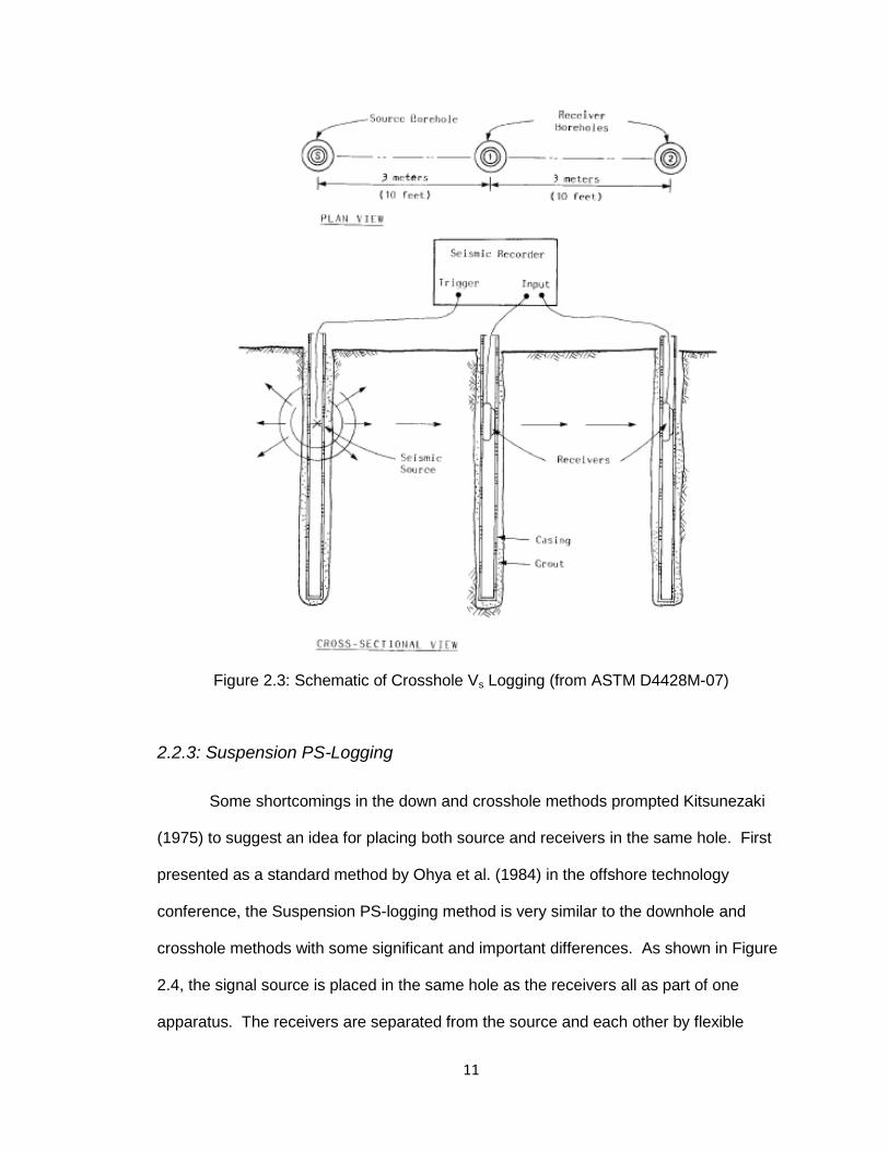
Figure 2.3: Schematic of Crosshole Vs Logging (from ASTM D4428M-07)

2.2.3: Suspension PS-Logging

Some shortcomings in the down and crosshole methods prompted Kitsunezaki

(1975) to suggest an idea for placing both source and receivers in the same hole. First

presented as a standard method by Ohya et al. (1984) in the offshore technology

conference, the Suspension PS-logging method is very similar to the downhole and

crosshole methods with some significant and important differences. As shown in Figure

2.4, the signal source is placed in the same hole as the receivers all as part of one

apparatus. The receivers are separated from the source and each other by flexible

12

tubing. The method requires that the logging occur below the water table as the source

creates a pressure wave in the borehole fluid that is then converted to seismic P and S-

waves at the borehole wall. The signals travel along the borehole walls until they are

converted back to a pressure wave at the receiver(s).

Figure 2.4: Schematic of Up-hole Suspension Logging Setup

(from GEOVision Geophysical Systems)

It is important to note that this is the only method that can image depths beyond

about 100m (limited only by borehole depth) with only one hole. In downhole logging,

the source is at the ground surface, meaning that the signal will attenuate at excessive

depths. While theoretically crosshole testing seems to be capable of also profiling

extremely deep, it is difficult to keep verticality of boreholes to such depths, and thus the

distance from source to receivers may change with depth (Ohya et al. 1984). Crosshole

13

testing also requires multiple borings, which quickly drive up cost. Casing installation is

optional, and it is often that better results are achieved with an uncased hole. This can

translate to significant saving in both time and cost. The suspension PS-logging method

can attain high resolution of up to 1m.

2.2.4: Seismic Cone Penetration Test (SCPT)

The SCPT method is almost identical to the downhole logging method. The

difference is that, rather than drilling and casing a hole for the receiver to be suspended

in, a geophone is placed inside a CPT probe as depicted in Figure 2.5, and

measurements can be made between intervals of a typical investigation. CPT trucks are

often outfitted with a shear beam, which is restrained by the weight of the truck itself.

Logging in this manner is limited by the inability to push the cone through overly stiff

material. For example, in cases where a cone is stopped due to a seam of dense sand

or gravel, it may be necessary to drill and use traditional downhole or suspension

logging to image strata below the problematic location.

14

Figure 2.5: Schematic of SCPT Vs Logging (from ASTM D7400-08)

2.3: Body Wave Methods

Body wave analysis methods such as Seismic Refraction and Reflection rely

upon the properties of P-waves traveling through strata of varying stiffness. Both

methods can be accomplished using standard geophones like the 4.5 Hz phones

employed by this study. This paper will focus primarily upon seismic refraction since it is

the body wave method implemented in this investigation and the concepts of reflection

are fairly similar.

2.3.1: Seismic Refraction

Accepted methods for data collection and analysis of Seismic Refraction are

provided in ASTM specification D5777 and Redpath’s overview in his 1973 paper

(Redpath, 1973). Simply put, the analysis compares the arrival times of refracted body

15

waves to that of the direct P-wave arrival along the ground surface along a linear array

of geophones. A typical array setup is shown in Figure 2.6.

Figure 2.6: Schematic of Seismic Refraction Array Setup (from ASTM D5777)

P-waves moving through a layered soil profile will refract at interfaces of differing

stiffness in accordance with Snell’s law. At the critical angle of incidence the wave will

be converted to a headwave, which moves along the interface between two strata of

different stiffness. This headwave then acts like a new signal source moving along the

interface at the rate of the higher stiffness material sending P-waves back up to the

receivers at the critical angle. Figure 2.7 depicts wave refraction at an interface and the

conditions for headwave generation.

16

Figure 2.7: Wave Refraction and the Critical Angle of Incidence (from Redpath 1973)

Snell’s Law is the relationship between wave speed in each medium and

refraction angle given by:

EQ 2.4

α = Angle of Incidence

β Refracted Angle

V1 = Wave Velocity in Incident Medium

V2 = Wave Velocity in Refracting Medium

and critical angle of incidence αc given at β 90°:

EQ 2.5

Due to the ability for the signal to move faster as a headwave in the stiffer

material, at some critical distance the refracted waves will reach the geophones at the

surface before the direct wave arrivals as shown in Figure 2.8. The figure depicts a

simple two-layer case with a bilinear distance-time curve whose slopes are equal to the

inverses of the wave velocity in each respective medium.

17

Figure 2.8: Schematic Showing First Arrivals from Direct and Refracted Waves with a

Corresponding Distance-Time Plot (from Redpath 1973)

If we consider the travel path ABCD shown in Figure 2.8, by simple mathematics

we can find the travel time to be given by the following expression:

EQ 2.6

Then, with simple geometry and Snell’s Law, we can find the depth to the refracting

surface Z1 from the following relationship:

EQ 2.7

Ti = Intercept Time as Shown in Figure 2.8

The full derivation of this equation can be found in many resources, including

Redpath (1973). It is possible to apply this same logic to profiles with more than two

18

layers, but the derivations are redundant and will not be addressed here. Another

method often used is the critical distance method; however, it follows the same general

logic as the previously described method and provides the same results. For this reason

the critical distance method will not be discussed here, however, a good discussion is

provided in Redpath (1973).

The examples to this point have explored horizontally layered profiles with source

points off one end of the array. If, however, the profile contains dipping layers, it

becomes necessary to analyze the distance-time curves from sources off of each end of

the array. As Redpath points out, the previously shown theory yields true velocities only

if the layering is horizontal. If this is not the case, this simplistic analysis will only yield

apparent velocities, and thus, erroneous depths. Figure 2.9 shows how the distance-

time curves are affected by the dipping beds.

Figure 2.9: Waves Refracting along Dipping Beds and the Corresponding Distance Time

Plot (from Redpath 1973)

19

If we take γ to be the dip angle of the interface, and α as the critical angle of

incidence for the refracting wave, the following relationships derived from Snell’s law

define the apparent refractor velocities up and down the array:

- EQ 2.8

EQ 2.9

and solving the system of equations the dip angle is found to be:

-

- -

EQ 2.10

Redpath goes on to explain that the true refractor velocity V2 is the harmonic

mean of the up and down array velocities multiplied by the cosine of the dip angle as

follows:

EQ 2.11

While this process adequately determines the true refractor velocity, the depth of

the refracting surface found by the intercept-time method is the depth of the projected

inclined plane below the shot point. The delay time method allows a depth calculation to

be made at each receiver and thus a much more detailed profile can be obtained.

20

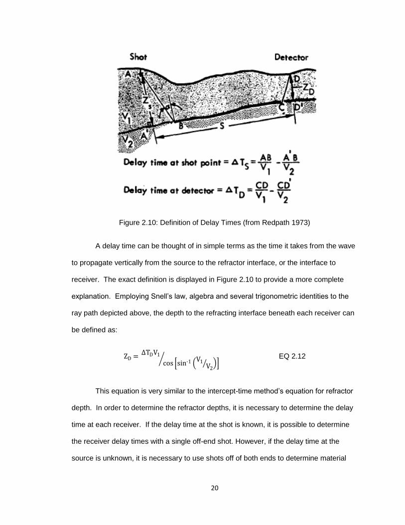
Figure 2.10: Definition of Delay Times (from Redpath 1973)

A delay time can be thought of in simple terms as the time it takes from the wave

to propagate vertically from the source to the refractor interface, or the interface to

receiver. The exact definition is displayed in Figure 2.10 to provide a more complete

explanation. Employing Snell’s law, algebra and several trigonometric identities to the

ray path depicted above, the depth to the refracting interface beneath each receiver can

be defined as:

-

EQ 2.12

This equation is very similar to the intercept-time method’s equation for refractor

depth. In order to determine the refractor depths, it is necessary to determine the delay

time at each receiver. If the delay time at the shot is known, it is possible to determine

the receiver delay times with a single off-end shot. However, if the delay time at the

source is unknown, it is necessary to use shots off of both ends to determine material

21

velocities and dip angles as previously described. The total delay time at shot and

receiver can be described by either of the following two equations:

EQ 2.13

-

EQ 2.14

Tt = Total Travel Time

ΔTs and ΔTD Defined in Figure 2.10

The equations combine to define the detector delay time as:

-

- EQ 2.15

After determining true velocities and the dipping geometry of the strata through

the intercept-time method previously discussed, the delay time at each receiver can be

calculated using EQ 2.15. Inputting these values into EQ 2.12 then yields the refractor

depth beneath each receiver. For more layers and more complicated geometries the

analysis rapidly becomes nontrivial, however, the same concepts apply. Redpath

provides multiple examples of these principals at work in realistic applications in his

1973 paper.

2.3.2: Seismic Reflection

The seismic reflection method was developed in the US some decades after the

seismic refraction method to better resolve deep imaging for the petroleum and mining

industries (Parasnis 1986). The array setup is very similar to that of the seismic

refraction method and is depicted below in Figure 2.11. While the array setup for a

refraction investigation needs to be thought out carefully prior to implementation to

22

insure correct resolution and depth of imaging, reflection surveys are much more

standardized and can be employed in numerous situations. Refraction surveys are still

primarily used by engineers for very near surface imaging; however, for deeper imaging

reflection is preferable due to the reduced array length requirements. And while a

refraction survey is only capable of imaging to depths of approximately a fourth or fifth of

the array length, reflection surveys can image much deeper.

Figure 2.11: Schematic of Seismic Reflection Survey (Illinois State Geologic Survey)

This method relies upon wave propagation principals and boundary interfaces as

described in Lay and Wallace’s book “Modern lobal Seismology” (1995). At any given

boundary, depending upon the acoustic impedances of the media, the energy will be

partitioned into refracted and reflected waves accordingly. Should the angle of incidence

exceed the critical angle of refraction, all of the energy will be reflected at the interface.

Again, the seismograms are analyzed for break points of reflected and direct arrivals. At

times it can be very difficult to differentiate reflected from refracted arrivals. The

23

refracted arrival often appears as an elongated arrival in front of the reflected wave when

the waves have not had sufficient travel time to fully separate.

For near surface surveys, a refraction analysis does a better job of resolving the

weathered layer(s) since more of the energy is partitioned to refracted waves until a

large change in impedance ratio is encountered. However, for complicated subsurface

geometries where impedance ratios are highly variable in the near surface, it is possible

that reflection will provide better results and an easier analysis.

2.4: Surface Wave Methods

Surface wave methods utilize unique properties of Rayleigh wave propagation to

develop the shear wave velocity profile. Rayleigh waves, or the vertical component of

the ground roll phenomenon, are the resultant wave produced by P and S-wave

interaction at the edge of a halfspace (Lay & Wallace 1995). The wave propagation

mechanism is depicted in Figure 2.12. An important characteristic of Rayleigh wave

propagation is that they move at a phase velocity that is independent of frequency in a

uniform halfspace. This trait allows inferences to be made about the medium through

which the wave is moving based upon the dispersion of different frequencies. This is the

basis for all surface wave analysis techniques. It should also be noted that Rayleigh

waves move at a slower rate than body waves, allowing them to be parsed out on a

seismogram, and do not attenuate as quickly.

24

Figure 2.12: Schematic of Rayleigh wave Propagation and Particle Motion

Rayleigh wave techniques can employ both active and passive source signals.

Surface waves attenuate slower than body waves, and the longer the wave length, the

slower the attenuation (Park et al. 1999). Large wavelength waves created by

earthquakes can travel tremendous distances before attenuating and provide good long

wavelength passive sources of energy; however, the uncertainty in source location can

cause significant complexity in data reduction (Yuan 2011).

2.4.1: Steady-State Method

The steady-state method was the original basis for the Spectral-Analysis-of-

Surface-Waves (SASW) method. An electromagnetic shaker is used as a source, and

oscillates at the frequency (f) of interest. The array setup usually employs either two or

three receivers with equal source-receiver and receiver-receiver spacings (Jones 1958).

These spacing are manipulated until a steady-state wave form is achieved as shown in

Figure 2.13. Once this is achieved, the geophone spacing is equivalent to the

wavelength (λ), and the Rayleigh wave phase velocity can be calculated using the

following formula:

EQ 2.16

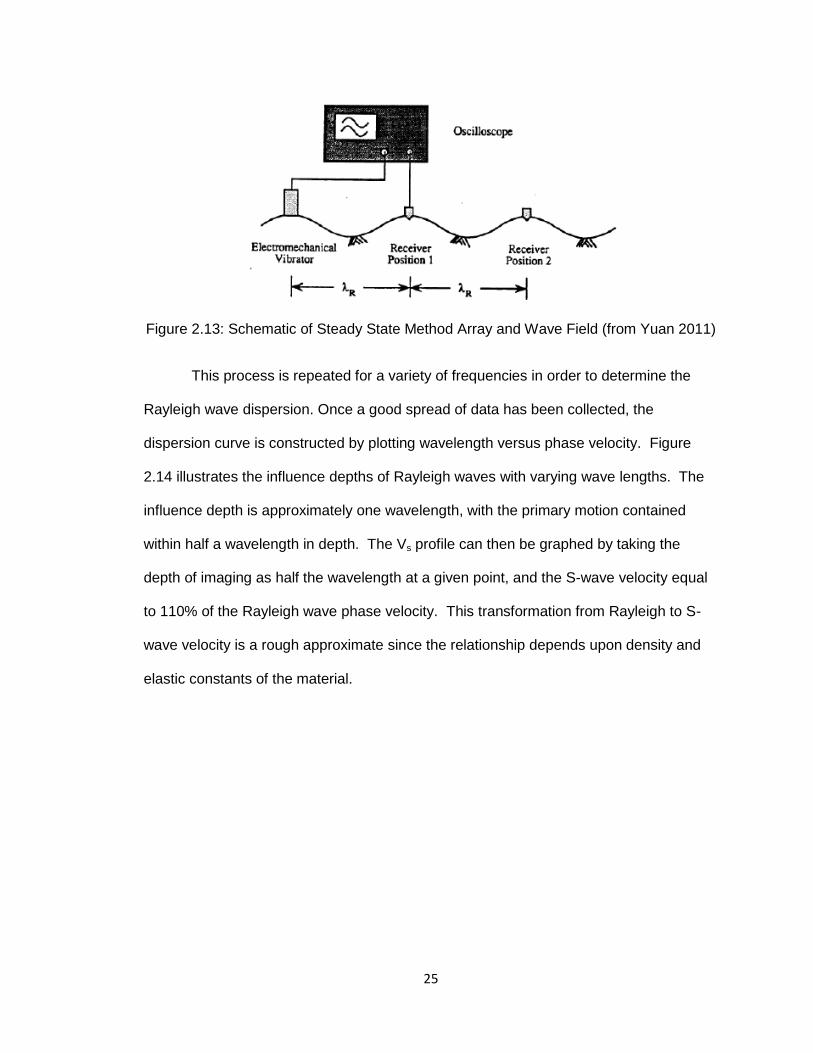
25

Figure 2.13: Schematic of Steady State Method Array and Wave Field (from Yuan 2011)

This process is repeated for a variety of frequencies in order to determine the

Rayleigh wave dispersion. Once a good spread of data has been collected, the

dispersion curve is constructed by plotting wavelength versus phase velocity. Figure

2.14 illustrates the influence depths of Rayleigh waves with varying wave lengths. The

influence depth is approximately one wavelength, with the primary motion contained

within half a wavelength in depth. The Vs profile can then be graphed by taking the

depth of imaging as half the wavelength at a given point, and the S-wave velocity equal

to 110% of the Rayleigh wave phase velocity. This transformation from Rayleigh to S-

wave velocity is a rough approximate since the relationship depends upon density and

elastic constants of the material.

26

Figure 2.14: Rayleigh wave Particle Motion at Varying Depths as a Function of

Wavelength (from Yuan 2011)

2.4.2: Spectral Analysis of Surface Waves (SASW)

Nazarian and Stokoe (1984) presented a more rapid and cost effective means of

developing an S-wave velocity profile by analysis of surface waves. The data collection

method is extremely similar to the steady state method, but simplified to reduce the labor

intensive procedure. The authors suggest that through a spectral analysis of Rayleigh

wave propagation it is possible to determine the S-wave velocity profile, and thus also

the shear modulus profile of a site. A typical array is displayed in Figure 2.15. By

inducing Rayleigh waves at a given source point, and then measuring the phase shift of

those waves between two receiver points, it is possible to find the wavelengths, and thus

the phase velocities. This is typically done with various receiver and source spacings in

order to capture the entire range of wavelengths. Longer wavelengths allow for deeper

imaging; however, receiver spacing must be between half and three times the

wavelengths being tracked in order to avoid spacial aliasing. Spacial aliasing occurs

when the receiver spacing is such that it does not adequately sample the wave being

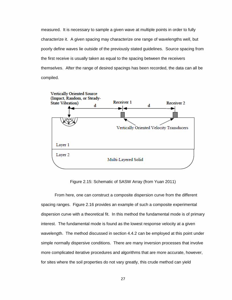
27

measured. It is necessary to sample a given wave at multiple points in order to fully

characterize it. A given spacing may characterize one range of wavelengths well, but

poorly define waves lie outside of the previously stated guidelines. Source spacing from

the first receive is usually taken as equal to the spacing between the receivers

themselves. After the range of desired spacings has been recorded, the data can all be

compiled.

Figure 2.15: Schematic of SASW Array (from Yuan 2011)

From here, one can construct a composite dispersion curve from the different

spacing ranges. Figure 2.16 provides an example of such a composite experimental

dispersion curve with a theoretical fit. In this method the fundamental mode is of primary

interest. The fundamental mode is found as the lowest response velocity at a given

wavelength. The method discussed in section 4.4.2 can be employed at this point under

simple normally dispersive conditions. There are many inversion processes that involve

more complicated iterative procedures and algorithms that are more accurate, however,

for sites where the soil properties do not vary greatly, this crude method can yield

28

reliable results. The authors present several case studies where the method is shown to

be very comparable to results obtained by cross or downhole testing to within 10%

(Nazarian and Stokoe 1984).

Figure 2.16: Example of Composite Experimental Dispersion Curve with Theoretical

Dispersion Curve Fit (from Yuan 2011)

2.4.3: Microtremor Analysis

The concept of using a microtremor analysis was originally explored by Aki

(1957) when he introduced the theory for the spacial autocorrelation method (SPAC).

He suggested that through combining knowledge of the wave spectrum in both time and

space one can obtain both the azimuth distribution of wave propagation and the

dispersion curve. The method employs autocorrelation between receiver signals at

29

different spacial coordinates. Combining this with a phase analysis yields a dispersion

curve and thus an indication of the medium through which the waves are propagating.

Tokimatsu et al. (1992) presented a new method of combining the use of ambient

microtremors and active sources to expand the frequency range of analysis. Tests like

steady-state or SASW rely completely on active sources, and it can be very difficult to

actively create surface waves of wavelengths significant enough to image below 10-

20m. On the other hand, while the use of microtremors had been previously employed

as a method for imaging very deep structure, ambient Rayleigh waves at high

frequencies have typically attenuated before reaching the array. A combination of active

and passive sources can take advantage of the utility of both methods. Table 2.1 lists

the methods available and applicable depth ranges.

Table 2.1: Applicability of Analysis Methods (from Tokimatsu et al. 1992)

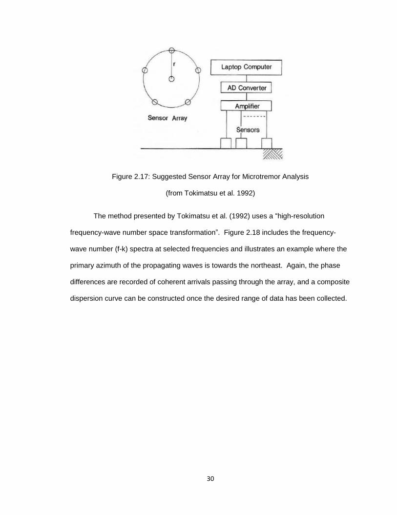
In order to resolve the azimuth of the microtremor arrivals in a passive analysis, it

is necessary to setup a two-dimensional array. Tokimatsu et al. (1992) suggest the

circular array presented in Figure 2.17 with varying diameters. As with receiver spacing

in a linear array, the diameter must be adjusted to record certain desired frequency

ranges and avoid spacial aliasing. The authors recommend starting at a 5m diameter

and doubling it repeatedly until all wavelengths desired have been correctly recorded.

30

Figure 2.17: Suggested Sensor Array for Microtremor Analysis

(from Tokimatsu et al. 1992)

The method presented by Tokimatsu et al. (1992) uses a “high-resolution

frequency-wave number space transformation”. Figure 2.18 includes the frequency-

wave number (f-k) spectra at selected frequencies and illustrates an example where the

primary azimuth of the propagating waves is towards the northeast. Again, the phase

differences are recorded of coherent arrivals passing through the array, and a composite

dispersion curve can be constructed once the desired range of data has been collected.

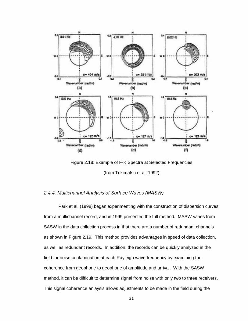
31

Figure 2.18: Example of F-K Spectra at Selected Frequencies

(from Tokimatsu et al. 1992)

2.4.4: Multichannel Analysis of Surface Waves (MASW)

Park et al. (1998) began experimenting with the construction of dispersion curves

from a multichannel record, and in 1999 presented the full method. MASW varies from

SASW in the data collection process in that there are a number of redundant channels

as shown in Figure 2.19. This method provides advantages in speed of data collection,

as well as redundant records. In addition, the records can be quickly analyzed in the

field for noise contamination at each Rayleigh wave frequency by examining the

coherence from geophone to geophone of amplitude and arrival. With the SASW

method, it can be difficult to determine signal from noise with only two to three receivers.

This signal coherence anlaysis allows adjustments to be made in the field during the

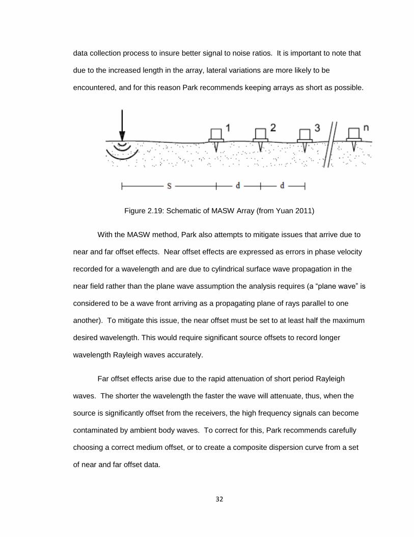
32

data collection process to insure better signal to noise ratios. It is important to note that

due to the increased length in the array, lateral variations are more likely to be

encountered, and for this reason Park recommends keeping arrays as short as possible.

Figure 2.19: Schematic of MASW Array (from Yuan 2011)

With the MASW method, Park also attempts to mitigate issues that arrive due to

near and far offset effects. Near offset effects are expressed as errors in phase velocity

recorded for a wavelength and are due to cylindrical surface wave propagation in the

near field rather than the plane wave assumption the analysis requires (a “plane wave” is

considered to be a wave front arriving as a propagating plane of rays parallel to one

another). To mitigate this issue, the near offset must be set to at least half the maximum

desired wavelength. This would require significant source offsets to record longer

wavelength Rayleigh waves accurately.

Far offset effects arise due to the rapid attenuation of short period Rayleigh

waves. The shorter the wavelength the faster the wave will attenuate, thus, when the

source is significantly offset from the receivers, the high frequency signals can become

contaminated by ambient body waves. To correct for this, Park recommends carefully

choosing a correct medium offset, or to create a composite dispersion curve from a set

of near and far offset data.

33

Park et al. (2005) presented a method of utilizing ambient surface waves as an

MASW source, and a way to mitigate near offset affects. Passive sources can be

assumed to be in the far field, thus even very long wavelength Rayleigh waves should

be propagating as plane waves. However, by itself, an ambient record would have

significant far offset effects present. The use of L-shaped arrays can allow the user to

resolve the azimuth of the passive signal arrivals. Figure 2.20 illustrates a combination

of passive and active records to develop a composite experimental dispersion curve.

Again, numerous forward modeling or inversion methods are available to fit a theoretical

dispersion curve to the experimental data.

Figure 2.20: Example of Expanded Frequency Range of Data from Combined Passive

and Active Records (from Yuan 2011)

34

2.4.5: Refraction Microtremor (ReMi)

Louie (2001) first presented the ReMi method of developing an S-wave velocity

profile. The intent was to develop a cheaper, faster and easier tool than those currently

available. While the method has received significant scrutiny, it has proven capable of

estimating average S-wave velocities to depths of up to 100m and within 20% accuracy

of more widely accepted measurement methods. Louie (2001) attempted to combine

the most effective aspects of the microtremor, SASW and MASW methods. The ReMi

method has gained acceptance today in many applications of shallow shear wave

velocity profiling. Despite relying upon passive signal sources, Louie (2001) indicates

that good results can be obtained with a simple linear array and typical seismic refraction

geophones (i.e. 4.5 Hz) and data acquisition systems. Another important characteristic

is that its primary reliance on passive source signals allows it to be utilized in an urban

setting where noise or body waves would drown out an active source signal.

2.4.5.1: Theory

Some important adjustments in data processing allow accurate results to be

obtained through the use of a linear array and passive signals. ReMi employs a

slantstack as described by Thorson and Claerbout (1985), also known as beam forming.

It is similar to a 2D Fourier-spectrum or f-k analysis, but with some differences that make

analysis simpler and more complete. Louie’s (2001) method is to take longer recordings

of as much as 50s and apply the slantstack to combine seismograms. The data is

analyzed through the p-f, or frequency-slowness, method originally suggested by

McMechan and Yedlin (1981). This method allows all phases to be included where an f-

k analysis would potentially alias data as shown in Figure 2.21. The dispersion curve

takes a unique slope in this space and thus is easily parsed out from body and air waves

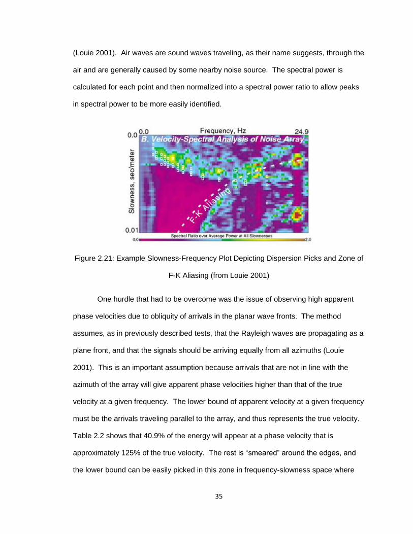
35

(Louie 2001). Air waves are sound waves traveling, as their name suggests, through the

air and are generally caused by some nearby noise source. The spectral power is

calculated for each point and then normalized into a spectral power ratio to allow peaks

in spectral power to be more easily identified.

Figure 2.21: Example Slowness-Frequency Plot Depicting Dispersion Picks and Zone of

F-K Aliasing (from Louie 2001)

One hurdle that had to be overcome was the issue of observing high apparent

phase velocities due to obliquity of arrivals in the planar wave fronts. The method

assumes, as in previously described tests, that the Rayleigh waves are propagating as a

plane front, and that the signals should be arriving equally from all azimuths (Louie

2001). This is an important assumption because arrivals that are not in line with the

azimuth of the array will give apparent phase velocities higher than that of the true

velocity at a given frequency. The lower bound of apparent velocity at a given frequency

must be the arrivals traveling parallel to the array, and thus represents the true velocity.

Table 2.2 shows that 40.9% of the energy will appear at a phase velocity that is

approximately 125% of the true velocity. The rest is “smeared” around the edges, and

the lower bound can be easily picked in this zone in frequency-slowness space where

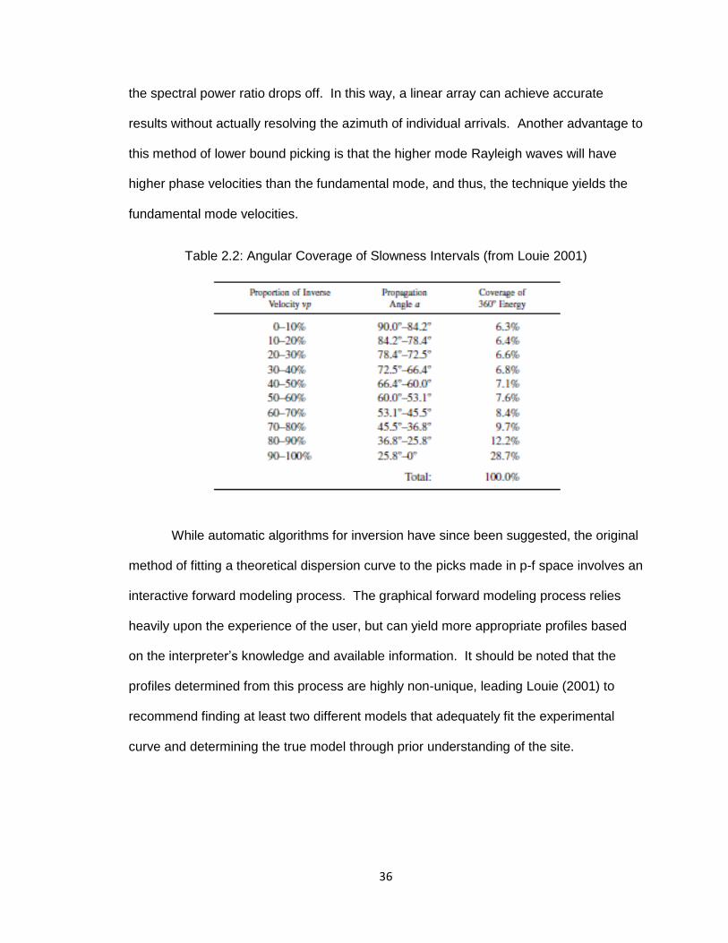
36

the spectral power ratio drops off. In this way, a linear array can achieve accurate

results without actually resolving the azimuth of individual arrivals. Another advantage to

this method of lower bound picking is that the higher mode Rayleigh waves will have

higher phase velocities than the fundamental mode, and thus, the technique yields the

fundamental mode velocities.

Table 2.2: Angular Coverage of Slowness Intervals (from Louie 2001)

While automatic algorithms for inversion have since been suggested, the original

method of fitting a theoretical dispersion curve to the picks made in p-f space involves an

interactive forward modeling process. The graphical forward modeling process relies

heavily upon the experience of the user, but can yield more appropriate profiles based

on the interpreter’s knowledge and available information. It should be noted that the

profiles determined from this process are highly non-unique, leading Louie (2001) to

recommend finding at least two different models that adequately fit the experimental

curve and determining the true model through prior understanding of the site.

37

2.4.5.2: Comparisons with other methods

As stated previously, the variability of the results both within the test method and

compared to other methods has caused some scrutiny. Louie (2001) compared his

newly developed method with others in 10 different sites and found that the shear wave

velocities could be found to within 20% accuracy to up to 100m depths of strata, and

suggest structure below that. Figure 2.22 depicts an example of inter-method variability

at a site in New Zealand. While Louie (2001) notes that ReMi cannot duplicate the detail

that downhole, crosshole or suspension ps-logging can provide; it does approximate

average velocities of 10-20m depth intervals very accurately.

Figure 2.22: Plot of Inter-method at Parkway, Wellington, New Zealand

(from Louie 2001)

In Spain, a group of geophysicists (Pérez-Santisteban et al., 2011) compared

ReMi, suspension PS-logging and SASW constructions of the shear wave velocity profile

under the railway embankment shown in Figure 2.23. This study had the advantage that

the profile was artificially constructed, and thus, highly controlled. The averaged results

from each method, plotted in Figure 2.24, showed that PS-logging provided the most

accurate profile followed by ReMi, and finally SASW. It is important to note that the ReMi

38

and SASW data required a fixed embankment depth in the inversion process in order to

yield the correct results. When the depth was unconstrained the methods produced

variable results. Unfortunately, the study was inconclusive as to the coefficients of

variation within each method for the same site.

Figure 2.23: (A) Placement on a Railway Embankment of SASW and ReMi Arrays with

Suspension PS-Logged Hole Shown at S-1 and (B) Cross Section of Embankment Soil

Profile (from Pérez-Santisteban et al. 2011)

Figure 2.24: Plot Illustrating Comparison between Methods on a Railway Embankment

(from Pérez-Santisteban et al. 2011)

39

2.5: Intra-method Variability

2.5.1: Variability within the ReMi Method

Due to the complicated assumptions and mathematics involved in ReMi paired

with wide variability of test results within the method, many are skeptical of the results

obtained. Cox and Beekman (2011) explore this variability within the test method itself

(not compared with true values). Much is assumed and unknown about the wavefield

analyzed in ReMi, thus, by comparing data obtained through different array orientations

and active versus passive signal sources, the authors attempted to determine the

degree of variability one could expect at a given site. The results shown in Table 2.3

indicate that the phase velocities at a given frequency could vary by as much as 85-

100% between passive and active sources. Orientation of the line of sensors showed

less impact on the results, as the active-active/passive-passive data groups tended to

agree with each other regardless of orientation. Figure 2.25 helps to emphasize the

degree of variation each variable can produce in the results. The variation that was

observed between orientations could be as much due to lateral change in soil strata as

to abnormalities in the wavefield.

Table 2.3: Intra-method Variability Analyzing Array Orientation and Signal Source

Influences (from Cox & Beekman 2011)

40

Figure 2.25: Plot Illustrating Comparisons of Array Orientation and Signal Source Type

(from Cox & Beekman 2011)

2.5.2: Intra-method Variability of Other Tests

This section is based upon Moss (2008), which investigates the intra-method

epistemic measurement uncertainty associated with a number of the methods discussed

in this chapter. This is a topic not widely explored. As the author points out, “There has

been little research to date evaluating the measurement uncertainty of individual tests

because of the amount of time and money required to run the tests…” This is an

important topic for engineers because the uncertainties involved in the analysis process

will compound upon the original inherent measurement uncertainty. Allowable stress

design and the use of factors of safety may at times be insufficient if the overall

uncertainty is large enough to allow a significant probability of failure (R. Moss, personal

communication, October 13, 2011). Despite the limited amount of data available to help

41

quantify these measurement uncertainties, Moss (2008) provides a basis upon which

future work can build a more robust dataset.

Moss (2008) segregates Vs profiling methods into two categories and suggests

preliminary coefficients of variation that can serve as tools to estimate the measurement

uncertainty associated with each. Those described as “invasive” methods correspond to

the tests described previously in this work as “direct measurement” methods.

Conversely, “noninvasive” methods refer to tests that do not involve placing source or

receivers at depth. In this case, the entire investigation occurs at the ground surface

such as those methods outlined in sections 2.3 and 2.4 of this chapter. The coefficients

of variation (standard deviation / mean) for these categories of measurement were found

to be on the order of 1-3% and 5-6% respectively. It should be noted, however, that the

noninvasive coefficient of variation refers specifically to the SASW method since the

others lacked the data to make any reliable conclusions. The paper presents

coefficients of variation for ReMi that are slightly lower than the range found for SASW,

but Moss (2008) points out that this may be an artifact of the small sample size.

42

Chapter 3: Testing Methods

The procedures and guidelines presented in this chapter are summarized from

the software manuals for SeisOpt ReMi v4.0, SeisOpt @2D v5.0 and Seismic Source

VibraScope.

3.1: Refraction Microtremor

The ReMi method consists of four primary steps. These include the array setup

in the field, data collection and exportation, data processing and, finally, forward

modeling.

3.1.1: Field Setup

In order to reduce complications in the analysis and in compliance with

recommendations by SeisOpt, the ReMi arrays employed by this study are all as near to

linear as possible. According to Optim, a 5% deviation in linearity will not affect the

accuracy of the method. It was occasionally necessary to record elevation data of the

receiver locations in order to adjust for the vertical deviation from linear; however,

horizontally speaking, all arrays in this study were within tolerable limits.

When using linear arrays, the ReMi method provides a 1D Vs profile at the

midpoint of the line by essentially averaging the profile along the array. For this reason,

when placing the array for a ReMi analysis, it is important to attempt to achieve a

placement approximately parallel to the feature of interest. Any change in the Vs profile

from one end of the array to the other will go unnoticed when looking at the condensed

1D profile yielded by the analysis. In this study, multiple arrays were situated on both the

hanging and footwalls approximately parallel to the anticipated locations of the fault

43

traces, and with varying offsets. Some judgment is necessary in determining the

approximate location of the fault trace. Given the known fault regime in the region, along

with a quick analysis of the geomorphic expression at the ground surface, it is possible

to develop a rough idea as to the likely location of the trace and place arrays

accordingly.

Once the array azimuth and starting point location has been determined, the

setup process can begin. Depth of accurate modeling is a function of the length of the

sensor array, and resolution is a function of the sensor spacing. As discussed in section

2.4.2, theoretically reliable data can only be collected for wavelengths between one third

the minimum geophone spacing, and twice the maximum receiver-receiver offset (overall

length of the array). The type of geophone is often the true limiting factor in maximum

imaging depth since low frequencies are necessary to image at depth and sampling is

very unreliable below the resonant frequency of the receiver. Sensors can be purchased

at varying resonant frequencies depending upon the needs of the project. Guidelines

provided by SeisOpt indicate that the maximum reliable imaging depth is approximately

1/2 to 1/3 the array length, and the resolution 1/2 to 1/3 the geophones spacing.

44

The equipment employed in this study includes the following:

1. 4.5 Hz single channel vertical motion geophones

2. Refraction cable allowing for 8m spaced connections to geophone split leads

3. DaqLink II Data acquisition hardware (Seismic Source)

4. Laptop with VScope software (Seismic Source) installed

5. Power source (12V Battery)

6. 10 and 16 lb sledge hammers

7. Piezoelectric trigger and cable extension

8. Metal striking plate

9. 100m measuring tape

When using 8m spacings, the cable itself can act as the measurement tool. For

other spacings, the measuring tape is used to set the line. The cable is then laid out as

close to linear as possible, with the connection points at the desired spacings. The

geophones are then placed at each connection point by planting the spike in the soil so

that it has a firm contact with the ground, especially in the vertical direction. If the

ground at the surface is loose or covered with plant matter, excavate to firmer material if

possible. The SeisOpt ReMi v4.0 User’s Manual states: “the geophones can be as

much as 15 degrees off vertical without compromising ReMi data quality.”

Once all geophones are situated, the cable can be connected to the DaqLink II

along with the power source and laptop. The array is now ready for data collection in

VScope.

45

3.1.2: Data Collection and Exportation with VScope

In order to correctly link with the data acquisition hardware, the laptop needs to

be disconnected on all network connections excepting the local port, which is linked to

the DaqLink II. It is also important to disable the firewall on the local network connection

which links to the data acquisition hardware. These steps can be completed in Windows

XP under Network Connections in the control panel. At this point, the DaqLink II is ready

to communicate with VScope.

It is best to begin a separate project for each array in order to maintain

organization. Select “New Project” from the “File” pull-down menu. Once a new project

has been created in VScope, the recording parameters can be verified and adjusted by

selecting “Device” from the “Options” pull-down menu. The window shown in Figure 3.1

should pop up and show the DaqLink. To adjust the settings, select the DAQ and click

the “DAQ Settings” button.

Figure 3.1: DAQ Setup Menu

The window shown in Figure 3.2 should appear, allowing configuration of the

data acquisition system. Under the “Acquisition” tab, insure that only the desired

channels are turned on. The channel settings shown in Figure 3.2 are adequate for this

46

type of testing. An acquisition time of 30s at 2ms intervals is adequate to provide good

resolution and capture a full spectrum of microtremors. Under the “Trigger” tab, “Auto

Trigger” should be selected in order to start recordings automatically when the “Start”

button is clicked on the main window. The “Order” tab allows adjustment of the order of

the traces in the records plot should multiple spreads be used. The normal setting is

typically correct, however, this can be checked by taking a recording with a signal

moving down the line to insure that the traces receive the signal in correct order. Once

these parameters have been set, select “OK”.

Figure 3.2: Data Acquisition Configuration Settings Window

47

On the main window recording is started by pressing the start button depicted in

Figure 3.3. The program should start recording and display that it is receiving in the

bottom left hand corner as shown in Figure 3.3. A good practice is to take a test

recording to insure that all channels are recording at approximately the same levels and

look reasonable. It is important not to induce any vibrations during this recording so that

the scale is not affected by the near channels receiving higher energy. Should any

traces appear abnormal, a quick inspection of the split lead connections to the cable,

and the seating of the geophone will typically solve the problem.

Figure 3.3: Scope Home Window Showing “Start” Button, Recording Status Bar, and

an Example Abnormal Trace Record

Upon verification that all traces are properly recording testing can begin.

Typically ten 30s recordings are sufficient to characterize a site. It is helpful at

48

particularly quiet sites to drive a vehicle back and forth off-end the array or walk along

the line (Louie, 2001). Striking a steel plate with a sledge hammer off-end of the array

provides another useful tool to enhance the higher frequency range of data. Higher

frequency waves attenuate more quickly, so this is typically the range where a more

remote site will be deficient of energy. If nearby traffic vibrations are available as a

source, the frequency range of the data can be improved by waiting for a particularly

large vehicle to approach to begin recording.

Once all desired recordings are made, the files need to be exported to a format

readable by the SeisOpt ReMi v4.0 software. To do this, select the “Open” button on the

home window near the top left corner. This will bring up the database of records as

shown in Figure 3.4. Each record needs to be exported individually in order to be

correctly read into ReMi Vspect v4.0. To do this, the desired record must be selected,

and then the second small icon in the top left corner will begin the exportation process.

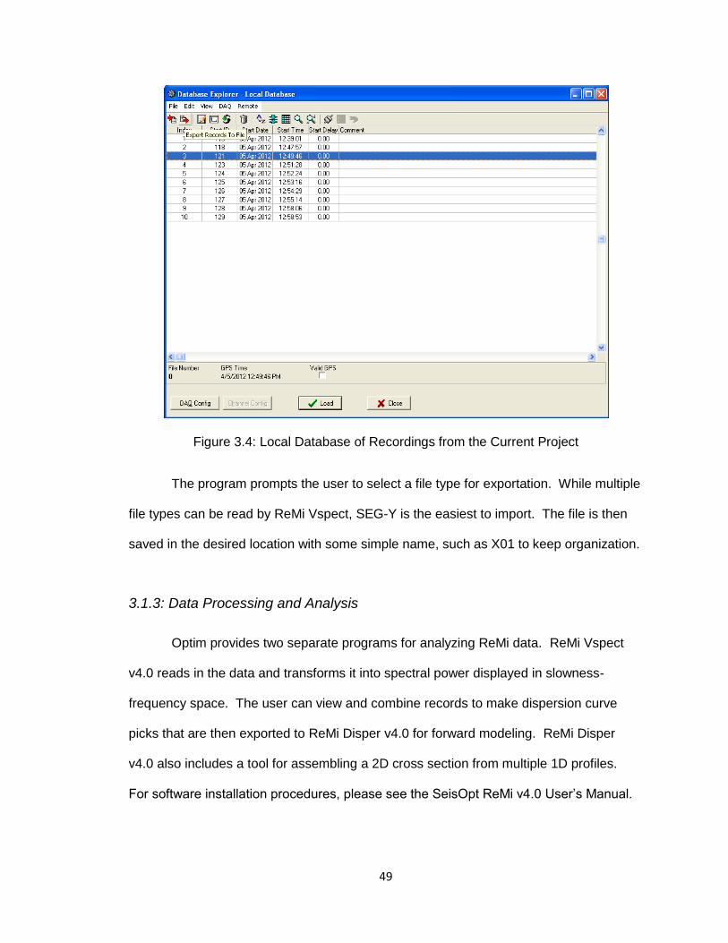
49

Figure 3.4: Local Database of Recordings from the Current Project

The program prompts the user to select a file type for exportation. While multiple

file types can be read by ReMi Vspect, SEG-Y is the easiest to import. The file is then

saved in the desired location with some simple name, such as X01 to keep organization.

3.1.3: Data Processing and Analysis

Optim provides two separate programs for analyzing ReMi data. ReMi Vspect

v4.0 reads in the data and transforms it into spectral power displayed in slowness-

frequency space. The user can view and combine records to make dispersion curve

picks that are then exported to ReMi Disper v4.0 for forward modeling. ReMi Disper

v4.0 also includes a tool for assembling a 2D cross section from multiple 1D profiles.

For software installation procedures, please see the SeisOpt ReMi v4.0 User’s Manual.

50

3.1.3.1: Processing Data and Making Dispersion Curve Picks in ReMi Vspect

v4.0

All data processing steps are located under the drop-down menu “ spect

Process” of each window. It is important to select the next step from the most recent

window opened to insure that all previous steps are included. SEG-Y data is read into

ReMi Vspect v4.0 by selecting “Step 1b: Open SE -Y Seismic Records…” on the

opening window. Once all desired files are selected and loaded, the window shown in

Figure 3.5 should appear, prompting the user for the data parameters.

Figure 3.5: ReMi Vspect v4.0 Data Reading Parameters

The easiest way to insure all data is read into the program from each record, the

values for first and last field record numbers to read are left blank. “Traces to Analyze”

should be from one to the number of recorded channels, typically either twelve or

twenty-four. The window in Figure 3.6 should appear after clicking “Read Binary File”,

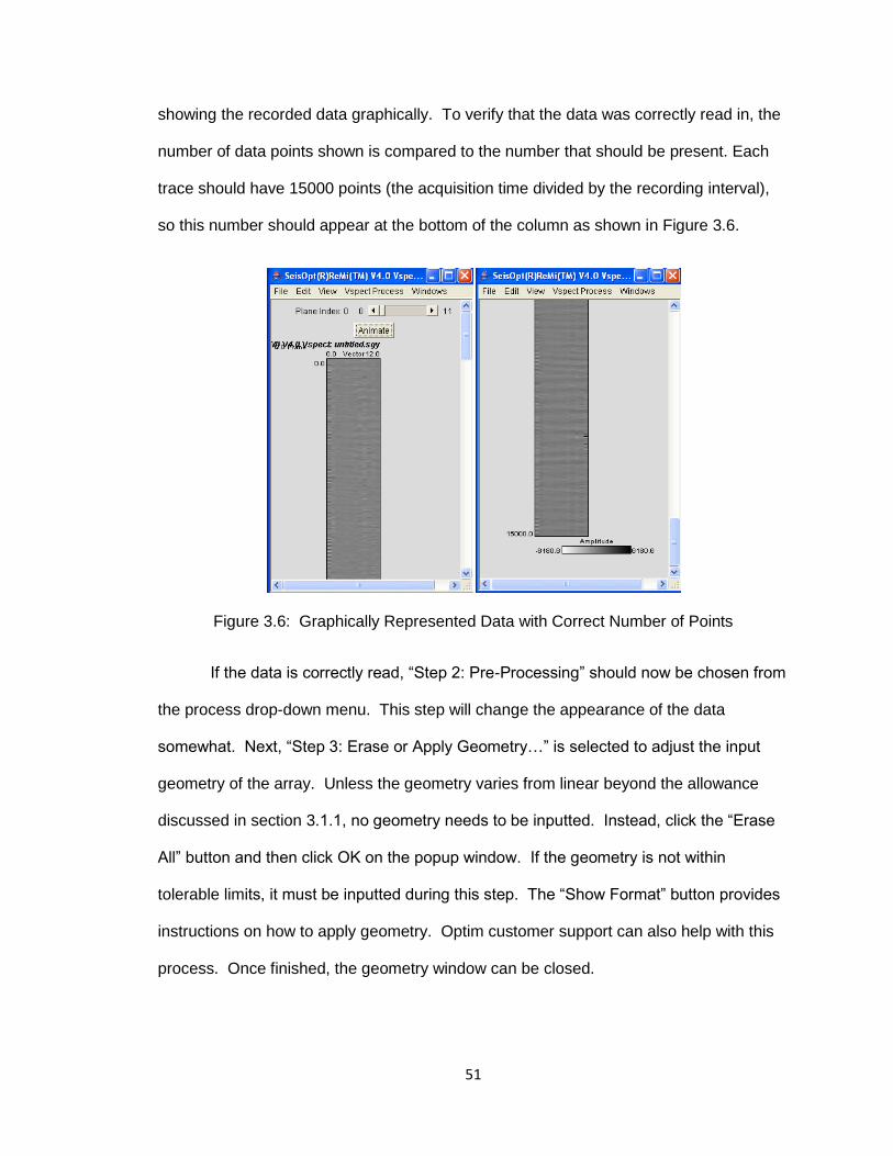
51

showing the recorded data graphically. To verify that the data was correctly read in, the

number of data points shown is compared to the number that should be present. Each

trace should have 15000 points (the acquisition time divided by the recording interval),

so this number should appear at the bottom of the column as shown in Figure 3.6.

Figure 3.6: Graphically Represented Data with Correct Number of Points

If the data is correctly read, “Step : Pre-Processing” should now be chosen from

the process drop-down menu. This step will change the appearance of the data

somewhat. Next, “Step 3: Erase or Apply eometry…” is selected to adjust the input

geometry of the array. Unless the geometry varies from linear beyond the allowance

discussed in section 3.1.1, no geometry needs to be inputted. Instead, click the “Erase

All” button and then click OK on the popup window. If the geometry is not within

tolerable limits, it must be inputted during this step. The “Show Format” button provides

instructions on how to apply geometry. Optim customer support can also help with this

process. Once finished, the geometry window can be closed.

52

“Step 4: Compute p-f of Each Record…” transforms the data into spectral power

in slowness-frequency space (p-f). The window in Figure 3.7 allows the user to adjust

the parameters of this transformation. “dt” is the sampling interval and “dx” the

geophone spacing. The maximum frequency of interest (Fmax) and the minimum

velocity of interest (Vmin) adjust the axes of the p-f plots.

Figure 3.7: p-f Transformation Input Parameters

It is important to note that the Fmax and Vmin parameters can also drastically

affect the appearance of the plotted data. The reason for this is that the program

actually plots the spectral ratio, or the normalized spectral power. This is done by

dividing the spectral power at each data point by the average spectral power in the

analysis space. By changing the size of the space that the program is analyzing, it is

also possible to significantly change the spectral ratios displayed. Because the p-f plots

depict anything above a spectral ratio of 2.5 as the same color (red), when the average

spectral power in the space is too low the plot will appear saturated in the response

53

regions. Conversely, if the analysis space contains a high average spectral power, the

ratios throughout the plots may not be high enough to clearly define the dispersion

curve. One must iterate through trial and error to find an ideal analysis space.

The process of iterating to find an ideal p-f space is highly dependent upon the

particular dataset, but the following guidelines work adequately in most cases. The

Fmax value should be determined first by varying the parameter up and down until the

user can fix it at approximately 0-5 Hz above the top frequency where the dispersion

trend is still apparent. In order to determine the Vmin value, the maximum slowness

(reciprocal Vmin) should first be set such that the bottom of the dispersion trend is just

captured in the analysis space. The interpreter should then decrease the Vmin value in

intervals of about 20Hz to determine if a better defined dispersion trend is attainable. A

higher Vmin allows better resolution, so the final space should be the highest value that

captures the entire dispersion trend and provides adequate spectral ratio peaks to make

reliable picks.

After finding an appropriate analysis space, the user must subjectively identify a

common trend between records of higher spectral ratios sloping generally down from left

to right (indicating increasing stiffness with depth). Sites that are not normally dispersive

(stiff over soft layers) may show an inversion in the dispersion curve slope, but typically

this downward slope can be expected throughout the plot. “Step 5: Combine Record p-

fs…” will stack the plots to help exaggerate this trend and help to reduce the prevalence

of random scatter. The resulting final plot can be greatly improved by excluding those

records that do not fit the trend the others show, or do not make sense given the known

local geology.

54

Making dispersion curve picks from the final combined p-f plot is made easier by

increasing the plot zoom size under the “ iew” drop-down menu. Picks are made by

left-clicking a pixel, and removed by right-clicking. As discussed in section 2.4.5.1, the

lower bound of the apparent phase velocities represents the true value, and can be

picked along the bottom edge of the trend of peak spectral ratios as shown in Figure 3.8.

Choosing points along the boundary between green and light blue shades is a good rule

of thumb. Multiple picks can be made at a given frequency to provide a bracket within

which the true value likely lies. The final picks are saved by selecting “Step 6: Pick and

Save Dispersion…” and choosing the file destination. The picks are now ready for

forward modeling in ReMi Disper v4.0. To save a JPEG of the p-f plot and picks, select

“Write JPE File…” from the “File” drop-down menu and choose the file destination.

Adding the file extension .jpg after the file name will allow the file to be more readily

opened by picture viewing software.

Figure 3.8: SeisOpt JPEG Output File after Making Picks on a Combined p-f Plot

55

3.1.3.2: Forward Modeling of a 1D Profile in ReMi Disper v4.0

After opening ReMi Disper v4.0, the saved picks are read into the program by

selecting “Load Picks…” from the “File” drop-down menu. To process data from ReMi

Vspect v4.0 the picks should be specified to be loaded from a dispersion file on the

following prompt. The program allows the user to then browse the hard-drive for the file

and loads the picks. The file path should appear at the top of the main window, and the

picks should appear as red dots on the velocity-period space at the bottom as shown in

Figure 3.9.

Figure 3.9: Model Profile Prior to Dispersion Curve Fitting Showing Experimental Picks

vs. Theoretical Dispersion Curve

56

From here, the model can be fit to the picks either manually or using the built-in

“Automatic Dispersion Inversion” tool located just above the dispersion plot. The most

rapid means of obtaining a reasonable fit is to employ the automatic inversion, then

refine the optimized model manually to reflect a reasonable approximation of the known

local geology. When the automatic inversion tool is selected, the window shown in

Figure 3.10 will appear with a number of modeling parameters. All of the parameters

affecting the profile space can be adjusted manually at the top of the home window.

Units should be consistent with those in the loaded picks. Most parameters can be

simply left as default; however it is often good to specify the number of layers desired in

the model and a maximum depth. A two or three layer model is sufficient for most data

sets. It is unreasonable to expect much more detail out of the ReMi method due to the

uncertainty in the picking process. The maximum model depth should be approximately

in accordance with the guidelines provided in section 3.1.1. A velocity inversion should

only be allowed in sites where stiff over soft layers are known to be present or the

dispersion picks clearly show existence of such structure. Once the parameters are set

the optimizer is run by pressing the button at the top of the window.

57

Figure 3.10: Automatic Dispersion Inversion Tool Parameters Window

Often the automated tool will give adequate results immediately. The operator

can try different maximum model depths and adjust the number of layers to try to find the

best model fit for the experimental data. If, after the optimizer has run, the curve still

does not fit the picks closely enough, the model can be manually adjusted by simply

dragging the pink velocity bars in each layer or the layer boundaries to more closely

match the data. The model fit is affected far more by Vs than density, so the default

density values are sufficient in most cases. This is a subjective and iterative process that

relies heavily upon user experience. The model fit is also highly non-unique, leaving it

up to the user to determine which profile makes the most sense. The displayed RMS

error beneath the dispersion curve plot can aid in the fitting process. When satisfied with

the model profile, JPEGs of the profile and dispersion curve can be exported from the

“File” drop-down menu. Again, appending .jpg to the end of the file name will make it

58

more readily accessed by picture viewing software. If the user desires to assemble a 2D

cross-section, a model file should also be exported from this same menu.

3.1.3.3: Assembling a 2D Cross-Section in ReMi Disper v4.0

When assembling a 2D Cross-section, ReMi Disper v4.0 will interpolate between

1D models to create a smooth 2D profile. If more than two models are included in the

2D assembly it is important that they all lay in approximately the same 2D plane. The

model file exported from each 1D profile must be edited to reflect the horizontal offset

relative to the others. To do this, the model file is opened in WordPad or some other text

editing program, and the first line of text reading “m,s” or “ft,s” is replaced by the

coordinates of horizontal offset and top elevation respectively. These values only need

to be separated by a single space. The first profile in the section should be set at a

horizontal value of zero, and all bottom-of-profile elevations should be modified to be

equal. Each model’s floor elevation is located in the last line of text in the first column.

The final model is clearer if the same number of layers is used in each model, and

velocities do not vary drastically from model to model within a given layer.

To assemble the sections, simply select “Create D Profile” from the “Tools” pull-

down menu on the main window of ReMi Disper v4.0. The program will ask the user to

choose the files of all models to be included. All files must be selected and loaded at

once, so all included models need to be in the same folder and selected simultaneously

by holding the control key. The “Next” button will bring up the profile parameters

window, allowing for selection of minimum and maximum elevation and velocity, as well

the pixel resolution on each axis. The “Smoothing” bar allows the degree of smoothing

between layers to be adjusted, representing gradually changing boundary velocities.

Once the desired parameters are set, the “Finish” button will assemble the model as

59

shown in Figure 3.11. The window may need to be expanded in order to properly view

the plot.

Figure 3.11: Example of a 2D Cross Section Assembled from Multiple 1D ReMi Profiles

The data from this file can be exported as an ASCII text file for importation into

Excel or other programs by choosing this option from the “File” drop-down menu. A

JPE of the plot can also be exported from the “File” menu.

3.2: Seismic Refraction

The seismic refraction method is made up of the same general steps of the ReMi

method. After array setup in the field the data must be analyzed to determine first break

points at each receiver and for each shot point record. These first break points and

60

survey geometry information are then exported to the modeling software to fit a profile to

the data.

3.2.1: Field Setup

The field setup for Seismic Refraction arrays is identical to the setup discussed in

section 3.1.1 with a few exceptions. It is important to note that array length needs to be

approximately three to five times the depth of desired imaging (Redpath, 1973). Due to

this restraint, without a large signal source, such as an explosive, it is difficult to image

depths more than 20-30m. The hammer and plate method used in this research does

not produce sufficient amplitudes to reach further than approximately 100m in ideal

conditions. In terms of resolution, Optim representatives recommend: “For -D

refraction horizontal resolution is about half geophone spacing, while vertical resolution

is about 0.375 times geophone spacing.”

61

One additional step in setup is to prepare the 10 or 16lb sledge hammer with the

piezoelectric trigger. The trigger should be taped securely to the top side of the handle

approximately 5cm above the head. The trigger cable can then be attached to an

extension cable and ultimately the DaqLink II. This trigger will queue the laptop to begin

recording.

3.2.2: Data Collection with VibraScope

The setup process for the acquisition software is very similar to that discussed in

section 3.1.2 with a few modifications and additional steps. Referring back to Figure 3.2,

the acquisition time should be set to 2 seconds, which is generally more than adequate

to capture full wave propagation down the entire array. 2ms sample intervals provide

decent continuous data sampling as well as reasonable record file sizes. The sample

interval can be set lower if desired for higher resolution of first break point definition.

Having a higher resolution can help immensely during the picking process. On the

“Trigger” tab, the option “Trigger on TimeBreak” should be selected with the default

settings.

With seismic refraction data, it is important to be able to track the first arrival of P-

waves at each receiver. The first arrival is often very difficult to separate from random

noise with only a single recording. It’s helpful to stack multiple records In order to

increase the amplitude of these arrivals and cancel some of the random noise. 5

records per shot point are typically sufficient, and more than 10 will not significantly

improve the data. To set the software to automatically stack records, select

“Preferences” from the “Options” pull-down menu at the top of the main window. The

window shown in Figure 3.1 should appear after choosing the “Auto Operation” tab.

62

Figure 3.12: Auto Operation Settings for Automated Seismic Refraction Data Collection

Recording is made easiest if the settings shown in Figure 3.12 are selected. The

number of records can be adjusted depending upon the needs of the project. It is

important to set the program to confirm before stacking and saving records to insure that

poor records are not included in the stack. When the setting “Auto Start Acquisition” is

turned on, the program will immediately wait for the next trigger signal to begin recording

after saving the previous record.

Optim recommends collecting records at a minimum of 7 shot points for 12

geophone arrays, or 14 points for 24 arrays. The locations of these shots for a 12

receiver setup are in plane with the array at twice the geophone spacing off of each end

of the array, and then at the midpoints between receivers 2-3, 4-5, 6-7, 8-9 and 10-11.

This same pattern is extrapolated for 24 receiver arrays. More source points will yield

better results during analysis; however, computation time will also be significantly

increased with more data to process.

63

It is important to be relatively precise with the shot point locations since travel

times are used to directly calculate velocities in each layer. It does not take a great deal

of difference in travel times to drastically change apparent velocities and cause

conflicting data between sources. After clicking the “Start” button on the home window,

the metal plate should be placed on the ground and firmly seated at the desired shot

location, then struck with the hammer. Given the settings described previously, the

program should record a shot with each strike of the hammer until the number of

recordings specified per stack have been recorded and accepted by the user. Once the

stack is complete, the user will be prompted to save the stack and input comments. This

is a good place to specify the location of the shot in order to maintain organization. This

procedure is repeated for each desired source point.

3.2.3: Data Processing and Analysis

Although Optim offers a program called SeisOptPicker that exports array geometry and

first break point picks in a data format compatible with SeisOpt@2D v5.0, there are

many disadvantages to its user interface. For this reason VScope is a preferable choice

for making picks. The data can be manually inputted into the text file formats required

by the modeling software without much extra effort, and there are a number of functions

that are far easier to access and use with Seismic Source’s software.

Once the data has been exported to SeisOpt@2D v5.0, the program can fit 2D models

of varying resolution to the data. The user can adjust experimental picks within the

program and iterate to develop the most reasonable and accurate solution.

64

3.2.3.1: Interpretation of Seismograms and Making First Brake Point (FBP) Picks

in VScope

VScope provides the user with a wide array of tools to help in analysis of the

seismograms. To open a stacked record to make picks, select the “Open” button in the

top left corner of the main window. The database will open, and the desired record is

opened by double-clicking it or selecting it and clicking “Load”. The first step is to

activate the picker module by clicking the icon for “Picker” to the top left of the plots. A

red line will appear at the top of each trace indicating that the program is ready to begin

picking. At this point it is helpful to right click in the plot space and select both “Scale”

and “Picks Table” so that the window appears as shown in Figure 3.13. These windows

help track the picks that are being made and allow the user to apply a variety of scale

options. The “Axis” window allows the maximum time values displayed to be adjusted

so that picks can be made more precisely and extraneous data excluded from the plot.

This window is accessed from either the icon near the top of the screen or by right

clicking the plot space and selecting “Axis”.

The best scaling option for this analysis is to apply Automatic Gain Control

(AGC). Depending upon the data, AGC may be adjusted to a wide range of values until

the FBPs are visible enough to be accurately picked. With good data and a relatively

quiet site this is often the only necessary adjustment in order to make precise FBP picks.

As the theory directs, the first arrivals at each trace should be chosen rather than

tracking a single wave signal across each trace. Picking the same wave through all

channels is essentially tracking only the direct arrivals and yields information only about

the velocity at the surface. Example picks are displayed at the red lines in Figure 3.13.

65

Figure 3.13: View of VScope Picker Module showing Scale Options, Picks Table and

Example First Break Point Picks

VScope also offers low cut, high cut and notch filters that are easily applied to the

data by simply toggling the icons just above the seismic plots. The frequency ranges for

these filters can be adjusted on the “Filters” tab of the “Preferences” window previously

accessed in section 3.2.2. It is preferable not to apply any filter to the data since doing

so can potentially cause the apparent FBP to move slightly. However, if the site is

particularly noisy, a high cut filter set to 80 Hz can help clean up those traces furthest

from the signal source and aid in making approximate FBP picks. Best practice would

be to make as many picks as possible without the filter, then turn it on only for the traces

that are difficult to analyze.

Once all picks are made for a record, they can be saved by selecting “Save

Picks…” from the “File” pull-down menu. Three files will be saved with extensions

66

_src.txt, _rec.txt and _obs.txt. Only the _obs.txt files need to be saved. This entire

picking process is then repeated for each source point.

3.2.3.2: Exporting for Processing through SeisOpt@2D v5.0

SeisOpt@2D v5.0 requires three separate text files as inputs. These files

contain the source location information, receiver location information, and the FBP picks

found in section 3.2.3.1. If the SeisOpt software

The source file is made up of three columns separated only by spaces or tabs.

The first column contains the horizontal distance along the survey line where each

source is located, the second describes the elevation, and the third indicates the number

of picks associated with each source (usually the number of receivers unless some

channels are neglected due to poor data). The units for both the source and receiver

files can be either in feet or meters.

The receiver file contains only two columns separated again by spaces or tabs.

The first column consists of the horizontal distance along the survey where each

receiver is located, and the second contains the elevation of each receiver. There must

be a receiver coordinate corresponding to each FBP pick, so the total number of rows

should equal the sum of the third column in the source file.

The file containing the pick times consists of a single column containing the FBP

for each receiver. The row number for a pick must be the same as the row number of its

corresponding geophone in the receiver file. The units can be either in seconds or

milliseconds.

Once the described text files have been created the data is ready to be processed into a

cross-section using SeisOpt@2D v5.0.

67

3.2.3.3: Creating a 2D P-Wave Velocity Profile Using SeisOpt@2D v5.0

Modeling in SeisOpt@2D v5.0 is a subjective process where many models of

varying resolution must be run to find the best optimization. Even after the best

resolution is found in the default uniform grid mesh, results can be further fine tuned

through several very involved methods that require significant user experience to

successfully yield improved results. For the sake of brevity, the procedure outlined here

is limited to the necessary steps in modeling a profile roughly (without any fine tuning).

Should the user wish to further refine a model, the SeisOpt@ D v5.0 User’s Manual

provides detailed guidelines to do so.

In order to import and process the data in SeisOpt@2D v5.0, open the program

and click “Cancel” when asked to browse for a file to open. An alert will inform the user

that the "pickfile" cannot be modified. The main window shown in Figure 3.14 will

appear. This is where the model profile will be viewed after being fit to the data. In

order to set up the modeling parameters, click the “RIOTS Settings” button to the bottom

left of the plot space. The window in Figure 3.15 should appear, asking the user for a

number of parameters for the input file.

68

Figure 3.14: Velocity Model Viewing Window

Figure 3.15: RIOTS Settings Window

69

For the first pass on a new data set, it is best to set the program to “Autocal” at

medium, high or highest resolution. Higher resolutions will typically yield better results,

however, the higher the setting the longer the analysis will take. It is also possible in

some cases that a “High” resolution setting will yield a better fit model than “Highest”.

The models obtained from these three settings should be compared, and the most

accurate fit should be the baseline resolution/grid mesh for subsequent runs. The unit

settings should be set to be consistent with those in the input files described in section

3. .3. . The “Browse” buttons allow the user to select the three input files, but it should

be noted that the program has difficulties with any path or filename that has a space in it.

This is a common issue with some tools in Optim programs in general, so spaces should

be avoided in file and folder names as a matter of course.

The “Horizontal Distances” box should be checked, the “Source Count” box

reflects the number of source points, and the “Pick Count” field specifies to the total

number of picks in the data set. For organizational purposes, a folder should be created

for the output directory so that the many output files do not clutter the @2D folder and

can be easily located. A file extension such as _autocal should be used to denote this

first run as the default resolution settings. It’s best to leave the “Set Iterations” box

unchecked so that the program will apply as many as necessary. The “Restart” and “Set

elocity” buttons only need to be checked for fine tuning.

When the “OK” box is clicked, a “riotsinput” file with the specified extension will

be saved to the chosen output directory. The “riotsinput” file without extension in the

2Dv50 folder will also be overwritten with these settings. It is this file without extension

that will be used as the input for the optimization. On the velocity plot window the red

“Run RIOTS” button begins the optimization process.

70

Should the process need to be terminated before complete, the task manager is

the preferable method of doing so due to a bug in the program that can cause the

computer to freeze if the “End/Terminate Process” button is pushed. The run time length

is dependent upon the resolution and size of the data set, as well as the processing

power of the machine. When complete, a number of files will be saved to the output

directory with the specified extension.

Once the best “Autocal” resolution model has been selected, subsequent runs

are still necessary. According to the Optim User’s Manual, “The default nz values that

are used when RIOTS is run using the default resolution settings (that is, when run at

‘High’, ‘Highest’ etc), is approximated one-third the maximum offsets in the survey. This

is not necessarily the one that will give you the best result.” To account for this, it is

recommended to run the optimization with the same values of hx, nx, and hz that were

used in the “Autocal” model, but with varying values of nz. Optim suggests reducing or

increasing the value by increments or decrements of 1 for each run with a minimum total

of 10 additional runs (5 decrements and 5 increments). This process can be automated

by creating a batch file using the tool provided in the “Set up Batch File” button.

The default values of hx, nx, hz and nz are found in the “riotsmsg” file with

extension corresponding to the model and can be opened in text editing software.

These values are then manually inputted in the “RIOTS Settings” window with the nz

value edited. A new extension must be applied to each settings file in order to keep

track of which is which and avoid overwriting. This process should be repeated for each

desired value of nz until all input files have been created. At this point the batch file is

created using the built-in tool.

71

When the “Set up Batch File” button is selected, a window will pop up asking the user to

specify the number of files to be included, and to browse for those files. After specifying

the number of files, pressing the “OK” button will refresh the window to reflect the new

number. The blank process window that appears can be closed. Each field is then filled

with a “riotsinput” file and the “OK” button will now set up the batch file named

“riotsbat.BAT” located in the Dv50 folder. To begin the batch processing, simply double

click this file.

Once the batch is completed, the RMS error associated with each can be found

in the “riotsmsg” files. Typically the lowest error corresponds to the best model;

however, the velocity plots should also be examined to insure that they make sense. To

view the velocity plots, click on the “Settings” button and choose the plots to be viewed.

The velocity plots are located in the files named “velfile_extension”. It is also helpful to

look at the files named “hitfile_extension” and “pickfile_extension”. The “hitfiles” shows

how many times each pixel was sampled by the data, and the “pickfile” displays the

experimental and modeled time-distance plots simultaneously. “velfile” and “hitfiles” are

both viewed using the “Interactive elocity raph” option, while “pickfile” requires the

selection “Model raph”. After clicking “OK”, user is prompted for the source, receiver

and observations files. Without selecting these, the user will not be able to modify the

experimental picks interactively on the “pickfile” plot. The plot to be viewed is selected

from the drop-down menu at the top of the window, and the “ o” button will bring up the

plot. When editing picks on the “pickfile” plot, changes are automatically saved to the

observations file after pressing the “Enter” or “Return” key.

72

Review of these plots will help the user determine which model is the best fit for

the data and known local geology. The “hitfiles” can be especially useful because they

display the ray coverage of the model space. Large gaps in ray coverage are modeled

with high uncertainty, so any resolution setting that outputs models exhibiting this

coverage deficiency can be eliminated.

Reducing the “Color Density” value on the drop-down menu in the top right

corner of the velocity plot viewing window to the number of expected layers will help to

illustrate the approximate interface locations. To more accurately locate these

interfaces, the green “DetLayer” button will open a module to aid in this process. Details

on the use of this module can be located in the user’s manual. This module was not

used in this body of work because it requires some knowledge about the layer velocities

to determine the layer depths.

A JPE of any of the plots can be readily obtained by using the “Make JPE ”

button to the left of the plot area. The user will be asked for the desired number of pixels

in the horizontal and vertical dimensions of the image. The

73

Chapter 4: Site Locations and Array Placement

Three sites local to San Luis Obispo were chosen for the testing in this project.

The suitability of each site will be discussed in the following sections as each was

chosen for different reasons. These include Crops Field C-31 of Cal Poly campus, the

Ingley site, originally named and trenched by Lettis and Hall (1994), and a third parcel

dubbed the Frontera site. The general locations of Crops Field C-31 and the Ingley site

are displayed in Figure 4.1. The Frontera site is not shown per the wishes of the land

owner.

Figure 4.1: Vicinity Map Depicting Ingley, and Crops Field C-31 Sites

74

4.1: Crops Field C-31

Crops Field C-31 was an ideal location to calibrate the data collection and

analysis process due to the locality and availability of subsurface data. Although no

known faulting is present at this site, it was a convenient location to run parametric

studies and learn the ReMi and Seismic Refraction methods in terms of the real world

application.

Subsurface information was readily available for Crops Field C-31 due to prior

geotechnical investigations. This work included SCPT soundings and borehole logs at

two locations as shown in Figure 4.2. The data from these investigations can be found

in Appendix A. This information proved helpful in comparing models obtained through

the ReMi and Seismic Refraction methods to the more accepted Vs profiles obtained

through SCPT soundings. The arrays were set near the prior investigations to minimize

lateral variation in the profile. Placement was limited by existing pavement and

extremely loose topsoil tilled for agricultural purposes. Loose topsoil would dampen any

signal significantly, and the equipment used in this research was not suitable for testing

on paved surfaces. The chosen locations of the arrays are shown in Figure 4.2 denoted

as CF-#. For a list of tests run at each array location, refer to Table 4.1.

75

Figure 4.2: Site Plan of Crops Field C-31 Depicting Array Locations as Line Segments

Table 4.1: Testing Schedule for Crops Field C-31 Arrays

Array # of Receivers Receiver Spacing Tests Run

CF-1 12 8m 3 Suites ReMi Seismic Refraction

CF-2 12 4m 1 Suite ReMi Seismic Refraction

CF-3 12 8m 1 Suite ReMi

CF-4 12 4m 1 Suite ReMi Seismic Refraction

*Multiple suites of ReMi imply that records were taken over multiple array deployments

in the same location. Each suite consists of a number of 30 second records at a time

step of 0.002s.

76

4.2: Ingley Site

The Ingley site was chosen for a number of reasons. The thrust faulting regime

of the Los Osos fault zone is coincides with our aim to identify lateral variation in the Vs

profile. This site was previously trenched as part of a fault investigation by Lettis and

Hall (1994). Our intention was to attempt to image the fault at a location with a known

geologic profile. The Irish Hills segment of the Los Osos fault zone shows particularly

good geomorphic expression allowing it to be thoroughly investigated in such locations

by trenching (Lettis and Hall, 1994). The information from this earlier study combined

with evident geomorphic expression served as guides for array placement.

4.2.1: Existing Information

Figure 4.3 depicts the site locations from the work of Lettis and Hall (1994) on the

Irish Hills segment of the Los Osos fault zone. The investigation involved trenching at

three separate sites near the intersection (not shown) of Los Osos Valley Road and W

Foothill Blvd. Unfortunately, many of the locations originally trenched in 1994 have since

been encroached upon by urban sprawl, leaving only the Ingley site as an accessible

testing area. Additionally, although trench T-1 of the Ingley site clearly identified lateral

variation in geologic structure, it sits adjacent to Sycamore Canyon Creek in a small

thicket of trees. The creek and trees surrounding T-1 make placement of arrays

problematic, leading to the decision to focus this study on trench T-2 of the Ingley site.

Figure 4.3: Detailed Geologic Map Showing Investigation Locations as well as Observed and Inferred Fault Traces (from Lettis and

Hall, 1994)

78

4.2.1.1: Trenching at Ingley Site T-2

Although T-2 does not expose the Franciscan Complex bedrock, it does capture

the primary fault trace, as well as evidence of older alluvium overlying younger as shown

in Figure 4.4. The trench is located on what Lettis and Hall (1994) identify as “a

prominent northeast-facing, 6-m-high topographic scarp”. The authors go on to offer

possible interpretations of the geomorphic and stratigraphic features in Figure 4.5.

These interpretations show a significant, though uncertain, offset in depth to bedrock

across this primary fault trace. Ideally, this offset would show up in geophysical data as

a noticeable difference in depth to bedrock or lateral stiffness across the fault.

Figure 4.4: Diagrammatic Log of Ingley Trench T-2 Showing Older Alluvium Thrust over Younger (from Lettis and Hall, 1994)

80

Figure 4.5: Possible Interpretations of the Overall Fault Behavior Based Upon Trench

Logs and Geomorphic Expression (from Lettis and Hall, 1994)

81

4.2.1.2: Geomorphology

Upon a preliminary site walk of the Ingley site, the scarp referred to by Lettis and

Hall (1994) was easily identified. Despite the present agricultural use of the land, the

scarp remains essentially intact with a small creek bed running along the length of the

toe. The topography to the northeast of the scarp is extremely flat, indicating that all

major faulting lies southwest of the feature. The level ground also made array

placement easier with no need for surveying elevation differences in receiver

coordinates. The site is generally located in close proximity to wetlands, which leads to

the conclusion (supported by Trench T-2) that soft recent channel deposits overlie the

young alluvium from late Pleistocene or Holocene eras.

4.2.2: Array Placement

Given the information from Lettis and Hall (1994) and preliminary site walks

investigating geomorphology and accessibility, the arrays were placed as depicted in

Figure 4.6. The creek running east to west is visible in the figure along the toe of the

scarp. Arrays I-1 through I-3 are located on the floodplain below the toe of the scarp, I-4

through I-6 are located on the scarp itself, and I-7 crosses the floodplain and climbs the

face of the scarp. Refer to Table 4.2 for array details.

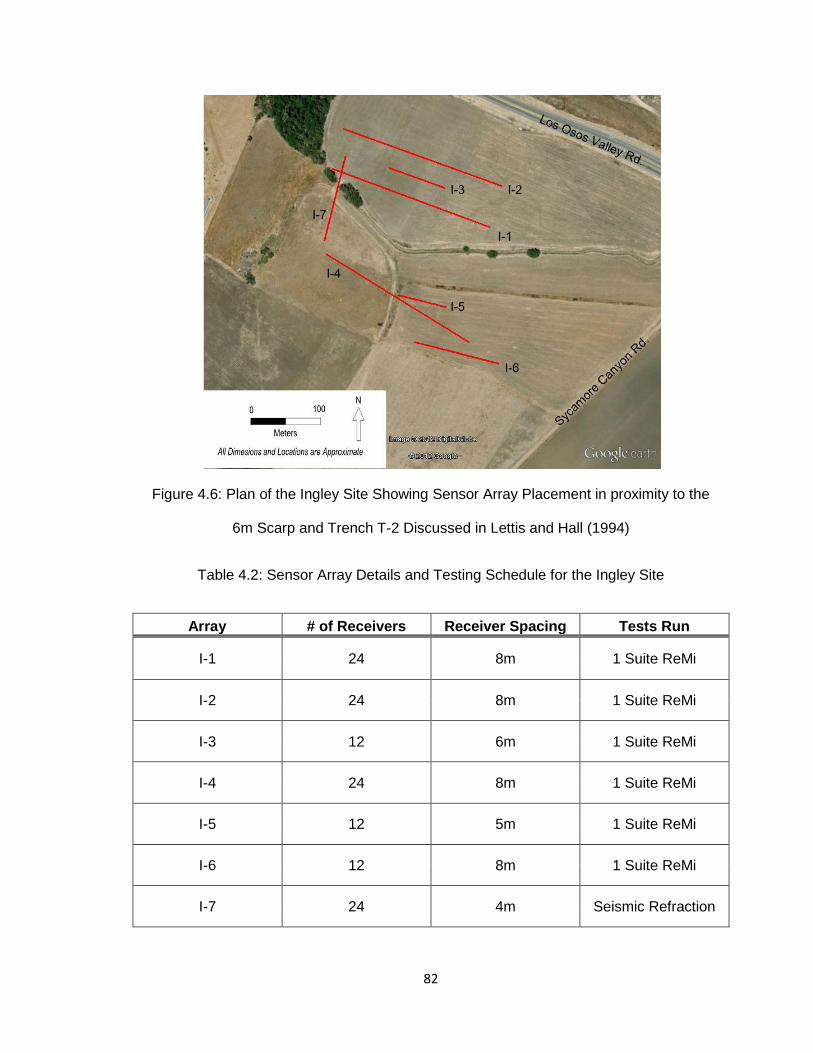
82

Figure 4.6: Plan of the Ingley Site Showing Sensor Array Placement in proximity to the

6m Scarp and Trench T-2 Discussed in Lettis and Hall (1994)

Table 4.2: Sensor Array Details and Testing Schedule for the Ingley Site


I-1 24 8m 1 Suite ReMi






I-7 24 4m Seismic Refraction

83

4.3: Frontera Site

The Frontera site was chosen as a location for attempting the ReMi and Seismic

Refraction methods to help find an unmapped fault trace with poor geomorphic

expression. This location has experienced little direct investigation, but Lettis and Hall

(1994) infer thrust fault traces in the detailed geologic map (figure not shown) printed

with their publication. The site lies where the Irish Hills structural sub-block appears to

begin to uplift on its eastern end.

4.3.1: Geomorphology

The site lies where the Irish Hills meet the floodplain of Los Osos Valley. Here there is

an immediate change in the topography that likely results from the uplift seen throughout

the Irish Hills section of the Los Osos fault zone. In preliminary site walks, the

geomorphic expression shown in Figure 4.7 was identified as the ideal place to focus the

attention of this work. The topography at this expression is not so extreme as to hinder

the ReMi or Seismic Refraction methods, and the surface material consists of sufficient

topsoil to develop good contact with the geophones.

4.3.2: Array Placement

During field work it was determined that the typical 8m spacing was yielding poor results,

so all arrays were spaced at 4m. This spacing seemed to improve the prominence of

the dispersion curve in the p-f plots processed in the field. 4m spacing also proved

necessary around the inferred scarp expression due to geometric constraints. Possible

reasons for the effect receiver spacing showed in the data will be discussed in Chapter

7. Figure 4.7 illustrates the array locations, and Table 4.3 provides array details and the

testing schedule.

84

Figure 4.7: Plan of the Frontera Site Arrays with a Recent Satellite Overlay Depicting the

Geomorphic Expression Identified in the Field in the Shaded Area

Table 4.3: Table 4.2: Sensor Array Details and Testing Schedule for the Frontera Site


M-1 12 4m 1 Suite ReMi

M-2a 12 8m 1 Suite ReMi

M-2b 12 4m 1 Suite ReMi




Seismic Refraction


Seismic Refraction


Seismic Refraction

85

Chapter 5: Crops Field C-31 Data Analysis

Crops Field C-31 was investigated through the deployment of four arrays as

shown on Figure 5.1 and described in Table 4.1. Array CF-1 was deployed in the same

location three separate times to assess the precision of the ReMi method. Array CF-2 is

also in approximately the same location and allows for a comparison with the records of

CF-1 to determine how much of an impact spacing of receivers may have upon results.

CF-2 also proved to be an ideal location to run a simple parametric study. The data from

array CF-3 yielded no clear dispersion trend, and CF-4 showed only slightly better

definition. Seismic refraction data was collected for all arrays except CF-3.

Figure 5.1: Site Plan of Crops Field C-31 Depicting Array Locations as Line Segments

86


All of the ReMi arrays deployed throughout this work collect data in 30s records

at a 2ms time-step. The data at Crops Field C-31 was expected to be fairly good due to

the presence of a multitude of ambient signal sources in the area. With the proximity of

Highland road, activities on Cal Poly campus and any agricultural work going on in the

neighboring fields, Crops Field C-31 seems an ideal location for passive data collection.

5.1.1: Highland Road Arrays

Despite the presence of plenty of ambient signal sources in the area, the p-f plots

obtained through multiple suites of testing along Highland road lacked good definition of

the dispersion trend. The spectral ratios along the typical slope of a dispersion curve

seemed “washed out” by the low-frequency artifact produced by the Fourier transform

that expresses the data in p-f space. The plots also seem to be highly saturated with

incoherent noise in the upper frequencies, possibly due to the presence of body waves.

Figures 5.2a-c show the p-f plots obtained through the three suites of data obtained

through array CF-1 and corresponding dispersion picks made along the lower bound of

the trend.

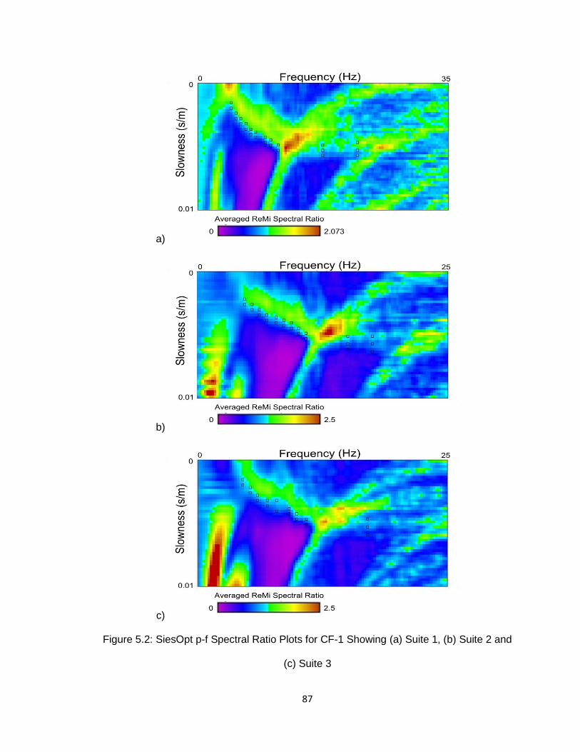
87

a)

b)

c)

Figure 5.2: SiesOpt p-f Spectral Ratio Plots for CF-1 Showing (a) Suite 1, (b) Suite 2 and

(c) Suite 3

88

The plots obtained from CF-2 will be discussed in section 5.1.1.2 as they

illustrate the results of a parametric study. They may be compared generally with the p-f

plots obtained from CF-1 in terms of the quality and definition of the dispersion trend, but

due to the offset in array midpoints and shorter array length lateral variation is an

uncontrolled variable. For this reason the results should not be directly compared with

CF-1 in the precision analysis discussed in section 5.1.1.1.

5.1.1.1: Highland Road Precision Study

The accuracy of the ReMi method has been tested by Louie (2001) and others in

relation to other more accepted methods such as suspension or downhole logging.

Literature on measurement uncertainty and repeatability within the method is less

prevalent, although Cox and Beekman (2011) investigate some aspects of the test. This

precision study here attempts to determine the repeatability of the ReMi method given

that the array location and orientation are held constant.

The data from the first trial was taken several months prior to the other two trials.

Trials two and three were taken on the same day with the third trial offset from the

second trial array by approximately 1/3 of a meter perpendicular to the line. Lateral

variation affects in this case should be negligible. While it is impossible to remove

human judgment entirely due to the need for dispersion picks from the p-f plots, the

profiles were modeled entirely by using the same automatic inversion algorithm for all

three trials. Each trial is specified to include three layers to a bottom depth of 30m.

While the profiles generated using solely the automatic algorithm may not be as well fit

to the data as it is possible to achieve manually, this was the best possible method to

develop a pseudo-blind comparison.

89

The results of the study are plotted in Figure 5.3 and summarized in Tables 5.1

and 5.2. Although trials two and three were taken on the same day and better controlled

in terms of receiver placement, the results differ as much between these trials as with

the first data set. The maximum percent difference in Vs30 between the three trials was

found to be 12.7% and the coefficient of variation (COV) is 7%. Statistical analyses for

each layer and interface appear summarized in Table 5.2 and suggest that at larger

depths and higher phase velocities the ReMi method is more stable. The coefficient of

variation in the bottom layer is less than half that of the top layer. Interface depths in this

study showed coefficients of variation on the order of 10-15%.

Figure 5.3: Vs30 Profile Illustrating Variance within the ReMi Method While Holding Array

Location and Orientation Constant

0

5

10

15

20

25

30

35

0 200 400 600 800 1000

De

pth

(m

)

Vs (m/s)

Trial 1

Trial 2

Trial 3

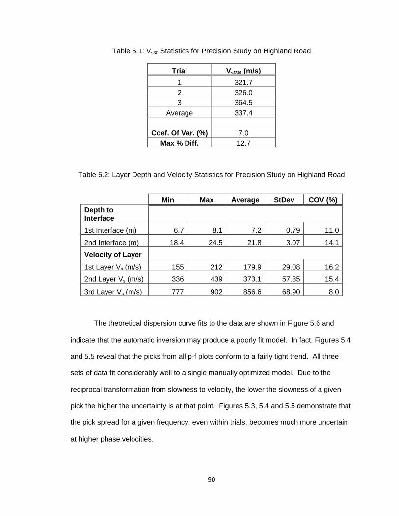
90

Table 5.1: Vs30 Statistics for Precision Study on Highland Road

Trial Vs(30) (m/s)

1 321.7

2 326.0

3 364.5

Average 337.4

Coef. Of Var. (%) 7.0

Max % Diff. 12.7

Table 5.2: Layer Depth and Velocity Statistics for Precision Study on Highland Road

Min Max Average StDev COV (%)

Depth to Interface

1st Interface (m) 6.7 8.1 7.2 0.79 11.0

2nd Interface (m) 18.4 24.5 21.8 3.07 14.1

Velocity of Layer

1st Layer Vs (m/s) 155 212 179.9 29.08 16.2

2nd Layer Vs (m/s) 336 439 373.1 57.35 15.4

3rd Layer Vs (m/s) 777 902 856.6 68.90 8.0

The theoretical dispersion curve fits to the data are shown in Figure 5.6 and

indicate that the automatic inversion may produce a poorly fit model. In fact, Figures 5.4

and 5.5 reveal that the picks from all p-f plots conform to a fairly tight trend. All three

sets of data fit considerably well to a single manually optimized model. Due to the

reciprocal transformation from slowness to velocity, the lower the slowness of a given

pick the higher the uncertainty is at that point. Figures 5.3, 5.4 and 5.5 demonstrate that

the pick spread for a given frequency, even within trials, becomes much more uncertain

at higher phase velocities.

91

Figure 5.4: Picks from All Precision Study Trials Plotted Simultaneously in Frequency-

Phase Velocity Space

Figure 5.5: Picks from All Precision Study Trials Plotted Simultaneously in Wavelength-

Phase Velocity Space

0

100

200

300

400

500

600

700

800

0 5 10 15 20 25

Ra

yle

igh

Wa

ve

Ph

ase

Ve

loc

ity (

m/s

)

Frequency (Hz)

Trial 1

Trial 2

Trial 3

0

100

200

300

400

500

600

700

800

1 10 100 1000

Ra

yle

igh

Wa

ve

Ph

ase

Ve

loc

ity (

m/s

)

Wavelength (m)

Trial 1

Trial 2

Trial 3

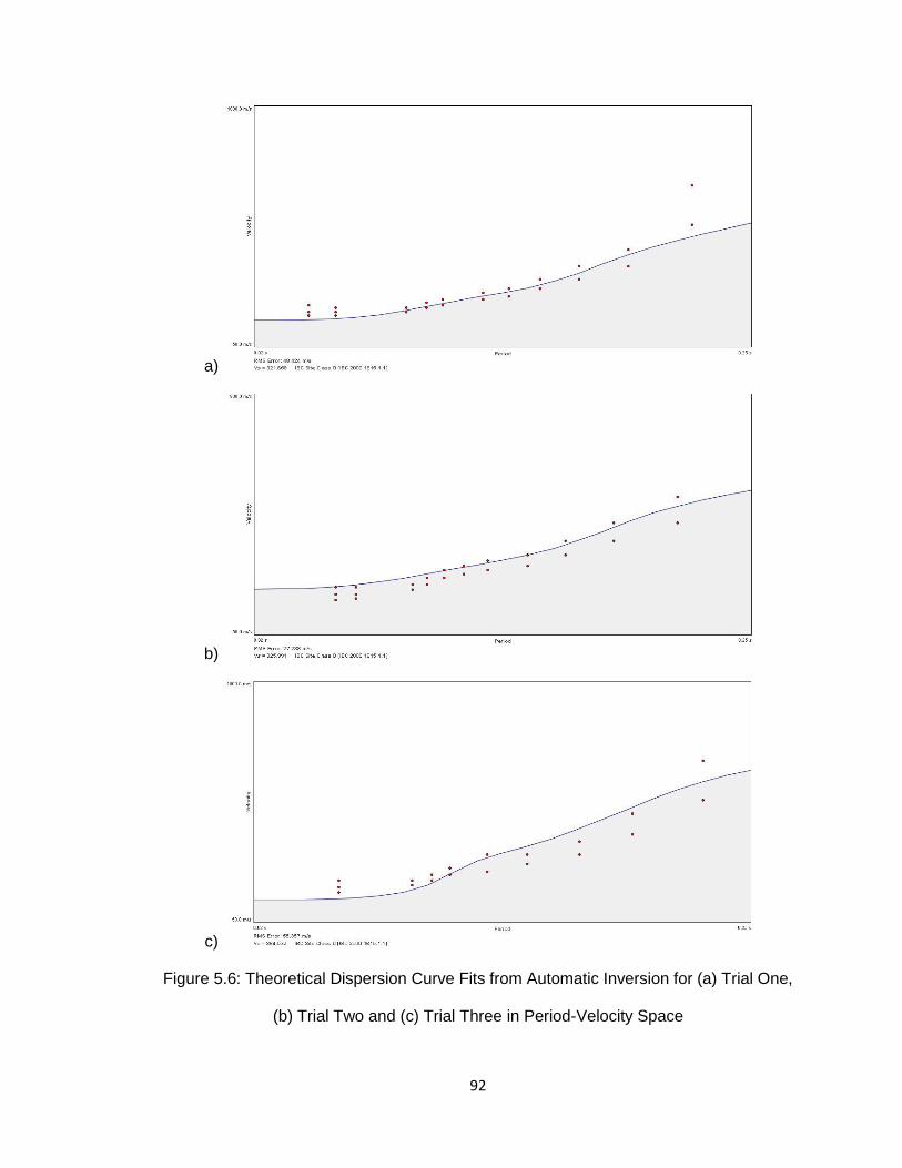
92

a)

b)

c)

Figure 5.6: Theoretical Dispersion Curve Fits from Automatic Inversion for (a) Trial One,

(b) Trial Two and (c) Trial Three in Period-Velocity Space

93

The point here is that, as Louie (2001) warns, the forward modeling process can

produce multiple models that fit the data equally well. Any lack of precision in the data

collection process in this study is far outweighed by the interpreter’s choices during the

forward modeling process. Poor choice of picks made on the p-f plots can lead the

interpreter incorrectly during the modeling process. This is why it is important to choose

multiple picks at a given frequency, attempting to bracket the possible range of values

within which the true slowness or phase velocity should lie. It is ultimately up to the

interpreter to make the call on what profile makes the most sense and to optimize the

model with this in mind.

5.1.1.2: Highland Road Parametric Study

ReMi array CF-2 was primarily used to run a parametric study. This tests the

affect that active signals coming from different azimuths and offsets have on the

transformed p-f plot. Figure 5.7 displays the results obtained through combined spectral

ratios from four ambient signal recordings. The dispersion trend is poorly defined with

very weak response in the lower frequency range and shows a wide distribution of

energy response along the mid and high frequencies. The wide distribution of energy

and poorly defined lower bound make the picking process uncertain at best.

94

Figure 5.7: CF-2 p-f Plot of Combined Passive Signal Records

By contrast, when introducing an active source, in this case sledge hammer

blows, the quality of the data can be much improved. Figure 5.8 helps to testify to the

difference that can be achieved. In this case, the signal source (10lb sledge on a steel

plate) was located off-end of the array approximately 10m. The range of frequencies

from approximately 25-35Hz shows a constant slowness across frequencies. This is

either indicative of a constant or near constant stiffness in the upper layers of the strata,

or is a product of some other response than that of a Rayleigh wave. Air waves can look

similar, but the phase velocity is considerably lower than the speed of sound.

95

Figure 5.8: CF-2 Recording with Hammer Blows on a Steel Plate Off-End of the Array

The hammer was then employed without the striking plate to evaluate the

difference in frequency range response. Figure 5.9 displays the results of the two

combined spectral ratio plots obtained during this activity. While it seems intuitive that

the steel plate would generate more high frequency content, the plots appear to show

the opposite. The steel plate response is much stronger in the mid-range frequencies,

where the direct strike to the ground surface showed much higher response in the

upper-range. Due to the nature of the spectral ratio display, the poorly defined low-mid

range frequencies may be a result of “wash out” caused by the strong response in the

upper range. When the term “wash out” is used in this work it is referring to the poor

definition of lower amplitude responses resulting from the spectral power normalization

that transforms the data to spectral ratios.

It is also possible that the upper frequency range is better lit in Figure 5.9

because of poor coupling and energy transfer between the plate and the soil surface.

The higher frequency waves will attenuate rapidly, thus the more energy that can be

transferred to the strata the better. The direct strike removes any contact issues,

96

however the reduced strike area can also reduce energy transfer to wave signals as a

result of plastic deformation in the soil (B. Cox, personal communication, July 4, 2012).

Figure 5.9: CF-2 Recording with Hammer Blows and no Plate Off-End of the Array

The records shown in Figure 5.10 attest to the effects of the plane wave arrival

assumption when the source is close to the array. When the receiver array is far enough

from the source, the radius is large and the difference in ray approach angles small.

With a source placed closely to the array the radius of the wave field is still small enough

that these approach angles will vary across the array such that the results are clearly

affected. As depicted in Figure 5.11, the closer the source, the more extreme the

difference in arrival times between the end geophones and those near the midpoint. The

further the array lies from the signal source the more closely together the receivers will

observe the signal.

The effect of a small radius source-array offset manifests itself in the p-f plots as

a marked shift in the steepness of the dispersion trend. When the source is further from

the array the angles of the arrivals with the line approach perpendicular, and the spectral

peaks indicate higher apparent velocities. A closer source will indicate lower velocity

spectral peaks, since the wave front arrives more obliquely, especially at the geophones

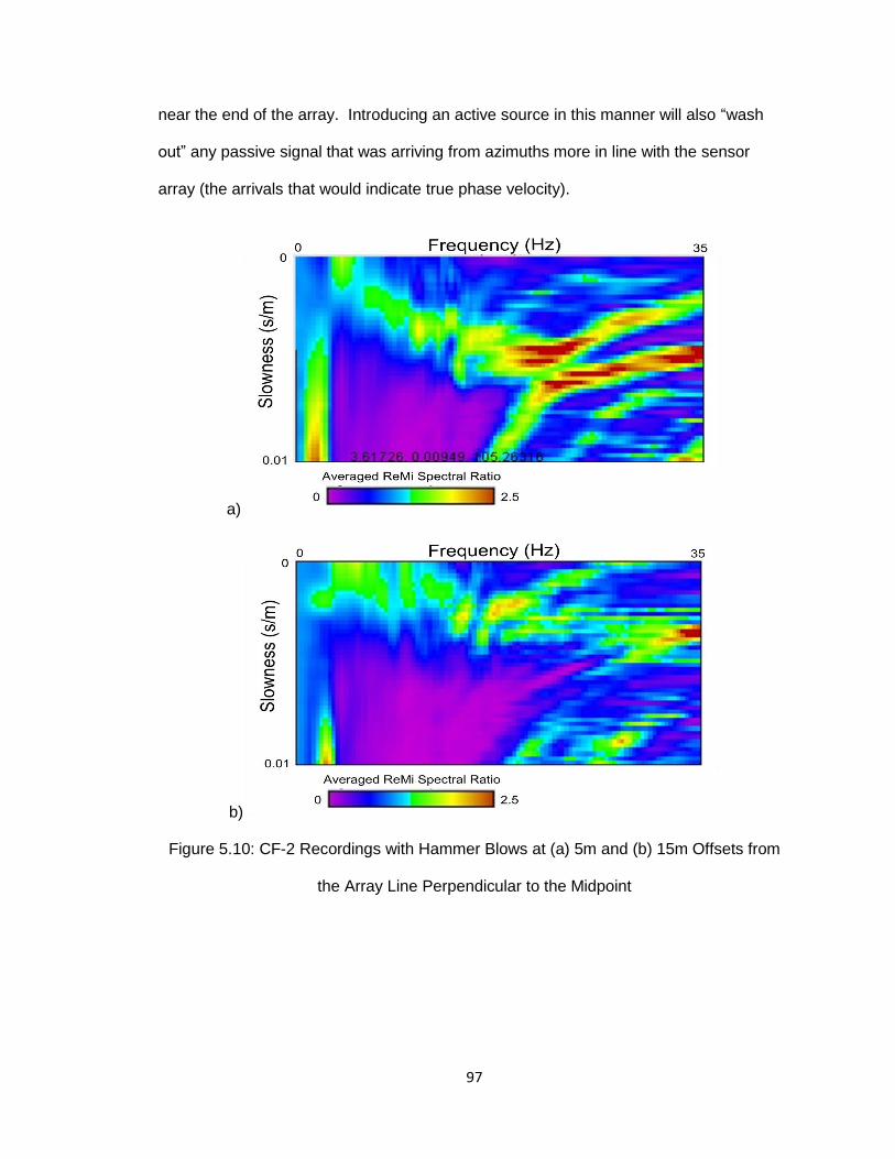
97

near the end of the array. Introducing an active source in this manner will also “wash

out” any passive signal that was arriving from azimuths more in line with the sensor

array (the arrivals that would indicate true phase velocity).

a)

b)

Figure 5.10: CF-2 Recordings with Hammer Blows at (a) 5m and (b) 15m Offsets from

the Array Line Perpendicular to the Midpoint

98

Figure 5.11: Diagram of Wave-Front Propagation from Sources Offset Perpendicular to

the Receiver Array

5.1.2: Stenner Creek Arrays

The ReMi data recorded along Stenner creek appears very poor in all records,

but combining some passive and active records on array CF-4 generates the plot shown

in Figure 5.12. The results from array CF-3 are unusable, and there are a number of

issues why this may be the case. The possible causes are discussed in section 5.1.3,

but it should be noted that arrays CF-3 and CF-4 were expected to provide better

dispersion trends given the perpendicular orientation of the lines to Highland Road. The

road should be providing the most energy of any local sources, and is off-end of the

array, which is ideal for defining the lower bound of the dispersion trend. The picks from

CF-4 were fit to a stiffness profile, and the results are discussed in comparison with

other available data in section 5.3.1.

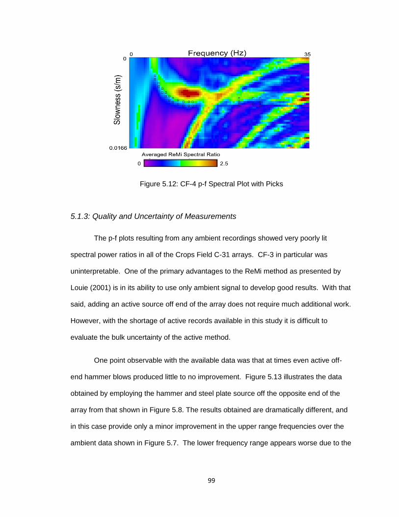
99

Figure 5.12: CF-4 p-f Spectral Plot with Picks

5.1.3: Quality and Uncertainty of Measurements

The p-f plots resulting from any ambient recordings showed very poorly lit

spectral power ratios in all of the Crops Field C-31 arrays. CF-3 in particular was

uninterpretable. One of the primary advantages to the ReMi method as presented by

Louie (2001) is in its ability to use only ambient signal to develop good results. With that

said, adding an active source off end of the array does not require much additional work.

However, with the shortage of active records available in this study it is difficult to

evaluate the bulk uncertainty of the active method.

One point observable with the available data was that at times even active off-

end hammer blows produced little to no improvement. Figure 5.13 illustrates the data

obtained by employing the hammer and steel plate source off the opposite end of the

array from that shown in Figure 5.8. The results obtained are dramatically different, and

in this case provide only a minor improvement in the upper range frequencies over the

ambient data shown in Figure 5.7. The lower frequency range appears worse due to the

100

“wash out” caused by the extreme peaks found in the 25-35Hz range. This observation

brings about questions as to the reliability from trial to trial of active source records.

Figure 5.13: CF-2 Recording with Hammer Blows on a Steel Plate Off-End of the Array

Symmetrically Opposite to the Data Shown in Figure 5.7

With geophysical testing, and especially the ReMi method, there are such a

multitude of uncontrolled variables that it is impossible to make definite conclusions

regarding the cause of the data anomalies. The remainder of this section will attempt to

highlight some possibilities.

The problems encountered with arrays CF-1 and CF-2 may possibly be attributed

to the presence of some man-made subsurface structure, or more likely, the presence of

buried utility lines. The amplitude plot of the twelve traces of CF-2 depicted in Figure

5.14 indicates that some type of interference is especially affecting traces 11 and 12.

The seismographs and frequency spectrum plot shown in figures 5.15 and 5.16 seem to

support this hypothesis. They clearly show traces 11 and 12 to be much more saturated

than the others, although the amplitudes are comparable. This is also the side of the

101

array the off-end source was located when data in the p-f plot shown in Figure 5.13 was

recorded.

The frequency spectrum plot shows a clear difference between channels at the

near end of the line and those near this interference. The frequencies above 80Hz show

a clearly stronger response with the interfering signal. While this is far higher than is

included on the p-f plots, there may also be significant lower frequency wave signals that

are not obvious on the frequency spectrum plot, but cause confusion during the data

transformation and in the wave signal coherence function. The high frequencies can be

filtered out, but the difference in the p-f plots appears negligible. There is evidence in all

four of the arrays at this site of some type of subsurface structure or utility interference.

Because electrical frequencies would show up around 60Hz and the site is located on an

agricultural field, the most likely culprit is the irrigation network.

102

Figure 5.14: Plot of Amplitude Recordings for Array CF-2 Indicating Interference in

Channels 11 and 12

Figure 5.15: Seismograms of Array CF-2 showing Interference Noise of a Possible Utility

Line along Highland Road

103

Figure 5.16: Frequency Spectrum Plot of Channels 1,2,11 and 12 for Array CF-2

Showing Differences in High Frequency Amplitudes

In the case of arrays CF-3 and CF-4, the data looked worse than that obtained

along Highland Road. This could have also been due to the utility line issue, the

proximity of the nearby slope down to Stenner Creek, or a combination of the two. An

array placed too closely to a steep slope may experience anomalies in the wave field,

especially in the lower frequencies. The break in the traveling medium can cause

changes in the way the waves propagate. The longer wavelengths require more space

laterally to insure that these effects will not be an issue.


The seismic refraction data was collected on arrays CF-1, CF-2 and CF-4. The

receiver and source diagrams are depicted in Figure 5.17. The hope was to learn the

seismic refraction method and also obtain some data that could be compared to the

historical SCPT and new ReMi data. Due to a number of reasons discussed in

subsequent sections, all goals were not met, but the process did provide a valuable

learning experience

104

Figure 5.17: Receiver and Source Coordinate Diagrams for (a) CF-1, (b) CF-2 and CF-4

5.2.1: Quality and Uncertainty of Measurements

The seismograms obtained during data collection on all of the Crops Field C-31

arrays turned out to be insufficient to make even approximate first break point picks.

The obvious proximity of Highland Road and the same utility interference experienced in

the ReMi data caused a very poor signal to noise ratio. The presence of this noise

coupled with large signal-receiver offsets did not allow good measurements to be made

of first break arrivals. Even using 4m receiver spacing, the larger offsets were enough to

attenuate the signal to the point that is appears untraceable on the seismograms. With a

larger hammer or an explosive as the signal source the quality of measurements could

be greatly improved. Stacking 5-10 records using the 10 lb sledge and the array setups

depicted in Figure 5.17 did help improve the data but was not adequate in this case.

a)

b)

105

5.2.2: Theoretical Travel Times

The modeling module of a software called Geogiga (www.geogiga.com) is

capable of providing theoretical travel time curves and seismograms for a given array

geometry and soil stiffness profile. This function seemed a useful way to constrain first

break picking in the data collected at Crops Field C-31. The input data was obtained

through density and shear wave velocity measurements taken during the prior CPT and

borehole investigations shown in Figure 5.1. This theoretical data was meant to only be

an approximation due to all the uncertainty involved in measurement, interpretation and

random error as well as spacial variability. Whether due to these uncertainties or other

causes, the theoretical and experimental data are so far from agreement that the initial

hope of constraining picks using theoretical data proved impossible. Figures 5.18 and

5.19 illustrate the poor quality of experimental data and the disconnect between the

theoretical and experimental first break points.

Figure 5.18: Experimental Seismic Refraction Seismograms Obtained with Source 8m

Off-End of CF-2

106

Figure 5.19: Theoretical Seismic Refraction Seismograms for the Area Adjacent to CF-2

It is plain at first glance that the theoretical and experimental data do not agree.

The same discrepancy was observed between experimental and theoretical data near

Stenner Creek. For this reason no model profiles are included with this work at Crops

Field C-31. Fortunately the other sites investigated in this research proved to have

much better signal to noise ratios. Despite the lack of results at Crops Field C-31, the

lessons learned aided in the subsequent testing at Ingley and Frontera.

107

5.3: Inter-Method Comparisons

Unfortunately the previous SCPT soundings were only performed to rather

shallow depths. Generally when ReMi has been compared with other methods it has

been shown to be adequate in its bulk approximations over large depth intervals. This

study showed a reasonable fit between the ReMi method and the SCPT data, maximum

depths of the CPT data were only about 11m and 18m. Profiles were initially modeled

blindly by using an automatic inversion algorithm, followed by manual manipulation to

obtain an optimal data fit. Additional models were also fit to the data after examining

the SCPT profiles and attempting to match them within the constraints of the dispersion

picks. The results shown in Figure 5.20 demonstrate the comparison of these results

and indicate that, especially when fitting data to a known profile, the results can be very

good.

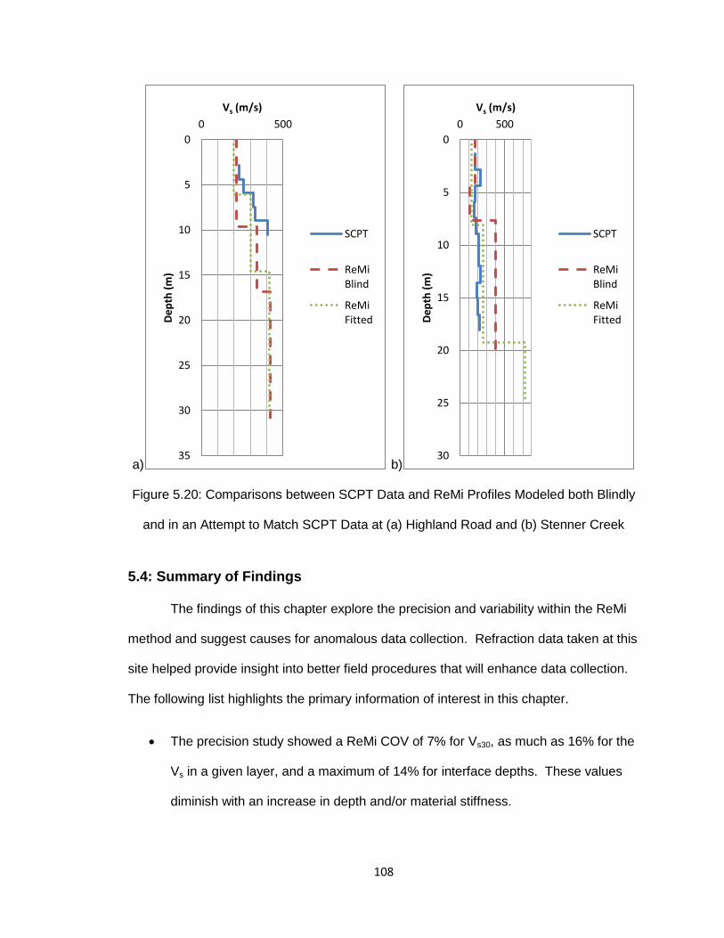
108

a) b)

Figure 5.20: Comparisons between SCPT Data and ReMi Profiles Modeled both Blindly

and in an Attempt to Match SCPT Data at (a) Highland Road and (b) Stenner Creek

5.4: Summary of Findings

The findings of this chapter explore the precision and variability within the ReMi

method and suggest causes for anomalous data collection. Refraction data taken at this

site helped provide insight into better field procedures that will enhance data collection.

The following list highlights the primary information of interest in this chapter.

The precision study showed a ReMi COV of 7% for Vs30, as much as 16% for the

Vs in a given layer, and a maximum of 14% for interface depths. These values

diminish with an increase in depth and/or material stiffness.

0

5

10

15

20

25

30

35

0 500

De

pth

(m

)

Vs (m/s)

SCPT

ReMi Blind

ReMi Fitted

0

5

10

15

20

25

30

0 500

De

pth

(m

)

Vs (m/s)

SCPT

ReMi Blind

ReMi Fitted

109

The parametric study indicated that off-line energy sources can cause a marked

increase in the apparent velocity of the dispersion trend due to the incongruence

with the wave field assumptions in the method.

The ambient records at this site showed very poor definition of the dispersion

curve, likely caused by the presence of irregular subsurface structure, incoherent

noise produced by utility lines, or physical clipping of the wave field by close

proximity slopes.

Blindly modeled profiles often disagree with those generated through other

methods, but when using previous knowledge as a guide very close matches can

be obtained.

Refraction data at this site indicated that, in close proximity to an ambient signal

source such as Highland Road, a much larger source is necessary to clearly

define first break points.

Stacking records, while effective in many situations, does not always act as an

adequate substitute for a larger energy source in seismic refraction testing.

Incoherent noise from utility lines or other sources can hamper seismic refraction

data collection.

Theoretical refraction data is very difficult to match to experimental data when the

lateral variation in the substrata beneath the array is largely unknown.

110

Chapter 6: Ingley Site Data Analysis

The goal of the work at the Ingley site was to make geophysical measurements

that corroborate the trench data and inferred local geology provided in Lettis and Hall

(1994). Although bedrock was never exposed in trench T-2 (Figure 4.4), the primary

fault expression was located. This Information suggests that some bedrock offset

should be present at depth along the trace. The trench also indicated that the hanging

wall consists of older alluvium thrust upon younger alluvium. The location of the trace

can thus be deduced by either locating an immediate and drastic shift in bedrock layer

depth, or by imaging significant lateral variation in bulk shear wave velocity.

This site allowed space around the scarp expression for laying out linear arrays,

both parallel and perpendicular to the feature. All array locations are displayed in Figure

6.1 and the testing schedule is located in Table 4.2. This site proved ideal for generating

2D ReMi profiles by interpolation between 1D sections.

111

Figure 6.1: Plan of the Ingley Site Showing Sensor Array Placement in proximity to the

6m Scarp and Trench T-2 Discussed in Lettis and Hall (1994)


The ReMi data collected at this site consist of results from six arrays parallel to

the scarp expression and perpendicular to trench T-2 of Lettis and Hall (1994). Three of

these arrays are located NE of the scarp on the inferred footwall. The remaining arrays

were placed on the inferred hanging wall. Space SW of the scarp on the hanging wall

was limited by agricultural activities. This Section concentrates on interpretation of the

p-f spectral ratio plots, 1D forward modeling and 2D assembled cross-sections.

Both this chapter and chapter 7 discuss the effects of vibrations caused

unintentionally by the field team and refer to this as a pseudo-active signal source.

112

Because the general location and type of source are known it is not appropriate to refer

to this energy as a passive signal (C. Wood, personal communication, October 5, 2012).

At the same time, these vibrations are not consistent with what is typically referred to as

an active signal because they were not intentionally generated at a measured location

with known frequency content.

6.1.1: Lower Arrays NE of Ingley Trench T-2

These arrays sit below the scarp expression on what appears to be a floodplain.

The elevation is approximately the same as that of the nearby wetlands just across Los

Osos Valley Road. Agricultural soil tilling has also made the topsoil in this location very

loose. The nearby road should act as a good signal source for testing at this entire site.

6.1.1.1: Individual p-f Spectral Ratio Plots and Picks

The three arrays produced similar p-f plots, but the definition quality of the lower

bound varies greatly between arrays. In general, well defined or not, the three arrays

agree well in the visible dispersion trend. Note that the slowness scale varies between

p-f plots in this chapter in order to obtain the best possible definition of the lower bound

spectral ratio trend.

Ambient recordings at the Ingley site contained the same frequency range

deficiencies that were observed in Chapter 5. Figure 6.2 displays the stacked ambient

recordings taken at I-1 demonstrating the lack of response above approximately 10Hz.

By contrast, even a small amount of pseudo-active energy produced the results shown

in Figure 6.3. Initially designated as an entirely passive recording, closer inspection of

the seismographs in Figure 6.4 revealed some unintentionally produced vibrations

originating at the array midpoint. This was the location of the data acquisition system,

113

which indicates that it was likely produced by incidental footfalls of the research team.

Rayleigh waves produced at the array midpoint in this manner would travel along the

array azimuth helping to strengthen the spectral ratios at the true phase velocity

boundary. It is difficult to say how the SeisOpt software handles this type of data given

the abnormalities in the coherence of the wave signal. Normally, a signal is tracked from

geophone to geophone through the array to determine its coherence, but this situation

would indicate two different coherent waves traveling in opposite directions and

originating spontaneously. One of the assumptions of the ReMi method is that the wave

signals are produced far enough away to arrive approximately as a plane wave,

approaching each receiver on the same azimuth.

Figure 6.2: p-f Spectral Ratio Plot of Ambient Signal Record for I-1

114

Figure 6.3: p-f Spectral Ratio Plot of Unintentional Mid-Array Vibrations Record for I-1

Figure 6.4: Seismographs of Unintentional Mid-Array Vibrations Record for I-1

Despite the uncertainty involved in allowing the power spectrum to be dominated

by an abnormal wave field, the resulting p-f plot does not indicate any gross anomalies.

In fact, the added energy seems to perfectly fill the frequency gap in Figure 6.2 along the

apparent lower bound that was previously poorly defined. The data presented in Figure

6.5 also agrees with this lower bound phase velocity trend. This p-f plot was produced

115

by combining records taken while signal was actively induced by intentionally walking up

and down the array. The dispersion curve response is strongest in this plot, but to

develop a more robust p-f plot (one that is representative of more records) the better

defined passive records were stacked in with those shown in Figure 6.5. Figure 6.7

displays the p-f plot and picks obtained from this stacking.

Figure 6.5: p-f Spectral Ratio Plot with Picks for Walking Record of I-1

Figure 6.6: Seismographs of a Walking Record for I-1

116

Figure 6.7: p-f Spectral Ratio Plot with Picks for Combined Active and Passive Records

of I-1

The plots in Figures 6.5 and 6.7 are very similar, but with minor variation around

13Hz and slightly better high frequency definition in the combined plot. When all picks

are plotted simultaneously, as demonstrated in Figure 6.8, the results are revealed to be

very consistent with one another.

Figure 6.8: Scatter of Picks from the Active and Combined Active/Passive p-f Plots

0

100

200

300

400

500

600

0 5 10 15 20 25

Rayle

igh

Wav

e P

hase V

elo

cit

y (

m/s

)

Frequency (Hz)

Active Only

Combined

117

Arrays I-2 and I-3 required the same stacking of active and passive records to

adequately define the dispersion curve lower bound. Unfortunately the data collected at

I-2 and plotted in Figure 6.9 contains numerous gaps in the trend. The data collected at

I-3 (Figure 6.10) exhibited a better defined dispersion, but this was only achieved by

reducing receiver spacing from 8m to 6m. The smaller spacing and shorter array may

have helped enhance the data by reducing lateral variation effects. A 24 receiver array

at 8m spacing spans 184m. This offset is easily large enough to introduce significant

lateral variation beneath the array that could cause disagreement over the Rayleigh

wave dispersion trend. If one end of the array indicates a different dispersion trend than

the opposite end, it may manifest itself in the p-f plots as a more widely smeared region

of spectral ratio peaks. This in turn could increase the average spectral power that the

plot is normalized by, and thus cause both dispersion trends to be poorly defined.

Another possible cause of the poor data at arrays I-2 and I-3 may be the

proximity of the road. The data collected at these three arrays looked significantly better

at each offset away from the road. I-2 showed the worst results and was the nearest to

the road. Again, given the number of uncontrolled variables, it is impossible to attribute

the symptoms to a specific cause with any certainty. The most likely and obvious cause

in this case is that the body waves (refracted P and S-waves) produced by the road may

be interfering with the Rayleigh wave analysis. At further offsets away from the road

these body waves would attenuate rapidly, hence the improvement in data quality with

distance from the road. This effect may not be noticeable at a site with other significant

signal sources that lie far enough away as to avoid body wave interference, but at a site

such as Ingley this is not the case. If the other ambient vibrations are significantly lower

in amplitude than the close proximity road vibrations, they will simply be “washed out” of

the spectral ratio plot.

118

Based on the results found here, placing an array in close proximity to a large

signal source with no other major energy sources in the area can produce poor results.

This could be easily investigated by testing more arrays at varying offsets in proximity to

a road with no other significant signal sources.

Figure 6.9: p-f Spectral Ratio Plot with Picks for I-2

Figure 6.10: p-f Spectral Ratio Plot with Picks for I-3

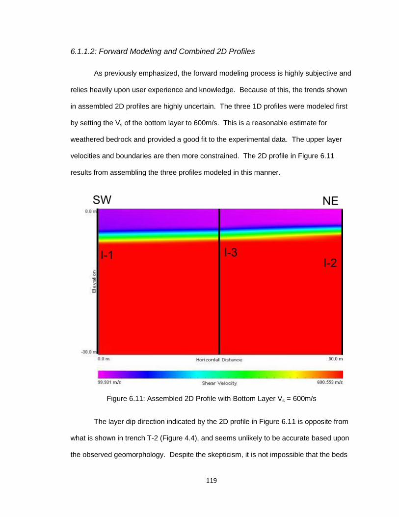
119

6.1.1.2: Forward Modeling and Combined 2D Profiles

As previously emphasized, the forward modeling process is highly subjective and

relies heavily upon user experience and knowledge. Because of this, the trends shown

in assembled 2D profiles are highly uncertain. The three 1D profiles were modeled first

by setting the Vs of the bottom layer to 600m/s. This is a reasonable estimate for

weathered bedrock and provided a good fit to the experimental data. The upper layer

velocities and boundaries are then more constrained. The 2D profile in Figure 6.11

results from assembling the three profiles modeled in this manner.

Figure 6.11: Assembled 2D Profile with Bottom Layer Vs = 600m/s

The layer dip direction indicated by the 2D profile in Figure 6.11 is opposite from

what is shown in trench T-2 (Figure 4.4), and seems unlikely to be accurate based upon

the observed geomorphology. Despite the skepticism, it is not impossible that the beds

120

do dip downwards toward the fault trace as a result of some subsidence of the footwall

under the hanging wall. To illustrate the degree of uncertainty involved in the ReMi

modeling process, the 2D profile in Figure 6.12 provided an equally good fit to the

dispersion pick data. This profile was created by setting the bottom layer depth to

700m/s, and by attempting to keep upper layer velocities close to equal in all three

models. After only allowing layer boundaries to move, a model such as the one shown

in Figure 6.13 fit well to each pick set. This is the model that is used in later

comparisons through this chapter because the dip direction of the deeper layer in this

trial seems more in agreement with trench T-2 (Figure 4.4).

Figure 6.12: Assembled 2D Profile with Bottom Layer Vs = 700m/s and Fit to Inferred

Geology in Lettis and Hall (1994)

121

Figure 6.13: Model Profile for I-1 Fit with Bottom Layer Vs = 700m/s

6.1.2: Upper Arrays on Scarp Expression near Ingley Trench T-2

The upper Ingley arrays are located directly on the scarp expression or hanging

wall and just at the top of slope. Elevation changes along array I-4 prompted an

investigation into its effect on the p-f plots. This section also attempts to explain why

arrays I-5 and I-6 both showed dual dispersion-like trends in their p-f spectral ratio plots.

Finally, the 1D model profiles are assembled into a 2D profile.

6.1.2.1: Array I-4 Slope Sensitivity Study

Array I-4 was situated across an erosion channel in the scarp expression.

Because of this, the midpoint of the array was located more than 5m below the highest

elevation receiver. Figure 6.14 provides a diagram of the array setup and the locations

of all receivers in vertical relation to one another. From the left end of the profile to the

low point there is a 5.9m elevation change over 88m. This equates to a 6.7% elevation

change, but there are locations where the grade is even steeper. Optim’s Refraction

Microtremor Field Tutorial (2006) indicates that up to 5% deviation from linear should not

affect the method’s proclaimed 15% accuracy window. This guideline is unspecific as to

122

other geometric possibilities, such as the lower midpoint in array I-4. Although not

outside the 5% threshold for the entire array length, portions of the array change at a

steeper grade, indicating that a geometry correction may be necessary in the analysis

process.

Figure 6.14: Array Elevation Profile for I-4 (no horizontal exaggeration)

Despite lacking any active source records for array I-4, the stacked ambient p-f

plots produced the dispersion trend displayed in Figure 6.15. Both the elevation

corrected and uncorrected plots are shown and appear to be very close to identical.

N

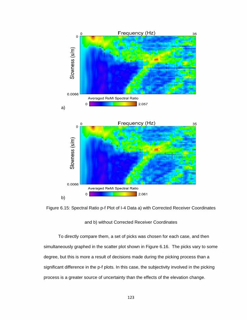
123

a)

b)

Figure 6.15: Spectral Ratio p-f Plot of I-4 Data a) with Corrected Receiver Coordinates

and b) without Corrected Receiver Coordinates

To directly compare them, a set of picks was chosen for each case, and then

simultaneously graphed in the scatter plot shown in Figure 6.16. The picks vary to some

degree, but this is more a result of decisions made during the picking process than a

significant difference in the p-f plots. In this case, the subjectivity involved in the picking

process is a greater source of uncertainty than the effects of the elevation change.

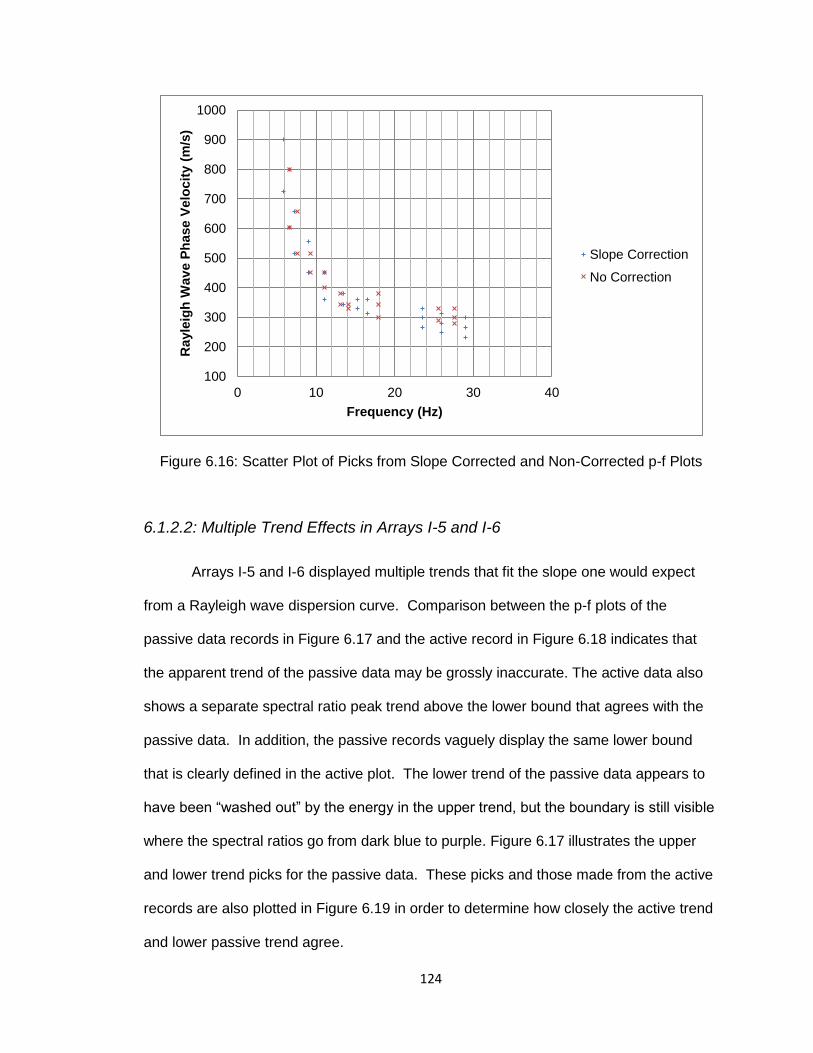
124

Figure 6.16: Scatter Plot of Picks from Slope Corrected and Non-Corrected p-f Plots

6.1.2.2: Multiple Trend Effects in Arrays I-5 and I-6

Arrays I-5 and I-6 displayed multiple trends that fit the slope one would expect

from a Rayleigh wave dispersion curve. Comparison between the p-f plots of the

passive data records in Figure 6.17 and the active record in Figure 6.18 indicates that

the apparent trend of the passive data may be grossly inaccurate. The active data also

shows a separate spectral ratio peak trend above the lower bound that agrees with the

passive data. In addition, the passive records vaguely display the same lower bound

that is clearly defined in the active plot. The lower trend of the passive data appears to

have been “washed out” by the energy in the upper trend, but the boundary is still visible

where the spectral ratios go from dark blue to purple. Figure 6.17 illustrates the upper

and lower trend picks for the passive data. These picks and those made from the active

records are also plotted in Figure 6.19 in order to determine how closely the active trend

and lower passive trend agree.

100

200

300

400

500

600

700

800

900

1000

0 10 20 30 40

Rayle

igh

Wav

e P

hase V

elo

cit

y (

m/s

)

Frequency (Hz)

Slope Correction

No Correction

125

a)

b)

Figure 6.17: Spectral Ratio p-f Plot of (a) Upper Trend and (b) Lower Trend Picks on

Passive Records for Array I-5

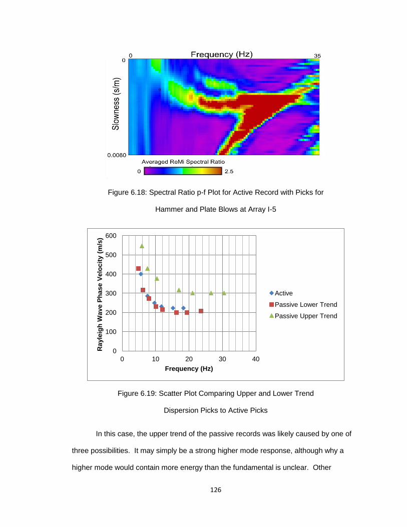
126

Figure 6.18: Spectral Ratio p-f Plot for Active Record with Picks for

Hammer and Plate Blows at Array I-5

Figure 6.19: Scatter Plot Comparing Upper and Lower Trend

Dispersion Picks to Active Picks

In this case, the upper trend of the passive records was likely caused by one of

three possibilities. It may simply be a strong higher mode response, although why a

higher mode would contain more energy than the fundamental is unclear. Other

0

100

200

300

400

500

600

0 10 20 30 40

Rayle

igh

Wav

e P

hase V

elo

cit

y (

m/s

)

Frequency (Hz)

Active

Passive Lower Trend

Passive Upper Trend

127

possibilities include the presence of an air wave response or sudden and significant

lateral variation in the soil strata beneath the array. The slowness range of the upper

trend is approximately consistent with the speed of sound, but there remains the

question as to where such a wave could have originated. There are no obvious passive

sources for an air wave in the vicinity. Sudden and distinct lateral variation in the soil

strata may also cause multiple dispersion curves by indicating a strong response along

one trend at one end of the array, and another strong response along the other trend on

the opposite end of the survey. It is possible that both are represented here. This was

the reason for aligning the array parallel to the feature of interest, but it is possible that

the geometry of the fault at depth is such that these efforts were unsuccessful. It is

impossible to say which of these possibilities, if any, is the culprit, but should the same

issue appear repeatedly with near-fault arrays, the lateral variability explanation seems

the most viable.

Array I-6 yielded a similar double dispersion trend as shown in Figures 6.20 and

6.21. In this case, stacking the passive records did yield a p-f plot with a clear lower

bound trend similar to that obtained by the hammer and plate active data displayed in

Figure 6.22. Although the lower trends do seem to agree, the scatter plot in Figure 6.23

of the picks from each case suggests that at lower frequencies the passive records

indicate a lower phase velocity, and at middle and upper frequencies the active case

shows a lower phase velocity. This is likely because the upper frequency data coming

from the sledge hammer has “washed out” a gap in the active record’s low frequencies.

In the middle and upper ranges the hammer signal dominates and the lower bound is

very tightly defined as opposed to the way it is smeared over a wider slowness range in

the passive case.

128

Figure 6.20: Spectral Ratio p-f Plot Showing a Typical Passive Recording at I-6

Figure 6.21: Spectral Ratio p-f Plot Showing Stacked Passive Recordings

and Picks at I-6

129

Figure 6.22: Spectral Ratio p-f Plot Showing Stacked Active Records and Picks at I-6

Figure 6.23: Scatter Plot of Active and Passive Record Picks for Array I-6

In terms of a cause for the double dispersion trend, the same possibilities that

were discussed with array I-5 remain plausible. Further data at the Frontera site may

help to isolate which cause is the most likely.

0

100

200

300

400

500

600

700

0 5 10 15

Rayle

igh

Wav

e P

hase V

elo

cit

y (

m/s

)

Frequency (Hz)

Active

Passive

130

6.1.2.3: Forward Modeling and Combined 2D Profile

Because of the elevation changes in I-4, it is difficult to compare its layer depths

to those of I-5 and I-6. Considering all the uncertainty already involved in the modeling

process I-4 was omitted from the 2D profile assembly. The experimental dispersion

picks at I-5 and I-6 were fit by setting the bottom layer velocity first, then adjusting the

upper layers until a close curve fit resulted. The layer velocities between the two 1D

model profiles were also adjusted to be consistent with one another, which further

constrained layer depths.

As discussed in section 6.1.1.2, the fit models are highly non-unique and could

change significantly when modeled with applying different criteria. The 2D assembly in

Figure 6.24 seems to be a reasonable model given the geomorphology of the scarp. It

indicates beds dipping down with the dip of the scarp. This could be accurate if the older

layers eroded away near the offset after uplift and then received newer deposits on top.

Figure 6.25 provides the layer depth and velocity details for the 1D model profile

generated from array I-6 data. The bottom layer velocity in this model is significantly

higher than those found in the arrays NE of the fault trace. Low frequency dispersion

picks, which sample deeper material, showed much higher phase velocities on the

hanging wall.

131

Figure 6.24: Assembled 2D Model Profile for Upper Ingley Arrays

Figure 6.25: I-6 Model Vs Profile

6.1.3: Comparison of Hanging and Footwall Profiles

The uncertainty in the forward modeling process makes identifying an offset in

bedrock very difficult. As has been demonstrated throughout this chapter, model profile

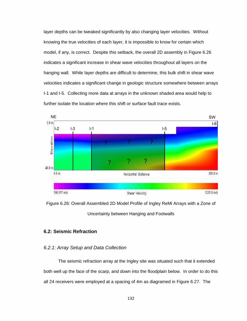
132

layer depths can be tweaked significantly by also changing layer velocities. Without

knowing the true velocities of each layer, it is impossible to know for certain which

model, if any, is correct. Despite this setback, the overall 2D assembly in Figure 6.26

indicates a significant increase in shear wave velocities throughout all layers on the

hanging wall. While layer depths are difficult to determine, this bulk shift in shear wave

velocities indicates a significant change in geologic structure somewhere between arrays

I-1 and I-5. Collecting more data at arrays in the unknown shaded area would help to

further isolate the location where this shift or surface fault trace exists.

Figure 6.26: Overall Assembled 2D Model Profile of Ingley ReMi Arrays with a Zone of

Uncertainty between Hanging and Footwalls


6.2.1: Array Setup and Data Collection

The seismic refraction array at the Ingley site was situated such that it extended

both well up the face of the scarp, and down into the floodplain below. In order to do this

all 24 receivers were employed at a spacing of 4m as diagramed in Figure 6.27. The

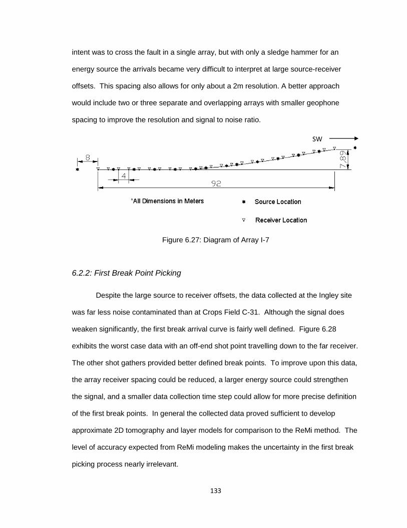
133

intent was to cross the fault in a single array, but with only a sledge hammer for an

energy source the arrivals became very difficult to interpret at large source-receiver

offsets. This spacing also allows for only about a 2m resolution. A better approach

would include two or three separate and overlapping arrays with smaller geophone

spacing to improve the resolution and signal to noise ratio.

Figure 6.27: Diagram of Array I-7

6.2.2: First Break Point Picking

Despite the large source to receiver offsets, the data collected at the Ingley site

was far less noise contaminated than at Crops Field C-31. Although the signal does

weaken significantly, the first break arrival curve is fairly well defined. Figure 6.28

exhibits the worst case data with an off-end shot point travelling down to the far receiver.

The other shot gathers provided better defined break points. To improve upon this data,

the array receiver spacing could be reduced, a larger energy source could strengthen

the signal, and a smaller data collection time step could allow for more precise definition

of the first break points. In general the collected data proved sufficient to develop

approximate 2D tomography and layer models for comparison to the ReMi method. The

level of accuracy expected from ReMi modeling makes the uncertainty in the first break

picking process nearly irrelevant.

SW

134

Figure 6.28: Off-End Shot Gather with First Break Point Picks at Array I-7

6.2.3: Model Profiles

When determining which 2D model resolution is the most appropriate, a good

way to start is by looking at the “hitfiles” showing the amount of times a given pixel has

been sampled. Many models can be quickly ruled out due to large gaps in the sampling

space. The program will often create artifacts or provide inaccurate velocities in these

poorly sampled regions. Figure 6.29 provides an example of a poor “hitfiles” plot,

whereas a slightly different resolution in Figure 6.30 shows excellent ray coverage. All

output plots from SeisOpt@2D in this work are in length units of meters and P-wave

velocity units of meters per second.

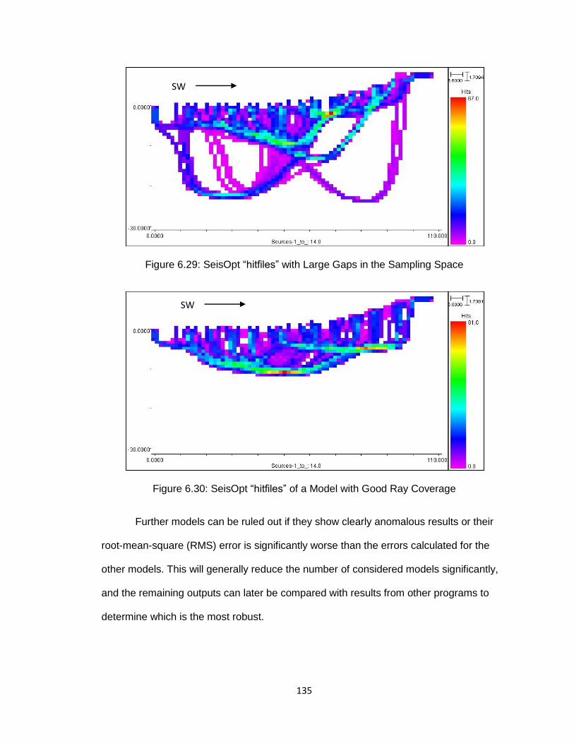
135

Figure 6.29: SeisOpt “hitfiles” with Large Gaps in the Sampling Space

Figure 6.30: SeisOpt “hitfiles” of a Model with Good Ray Coverage

Further models can be ruled out if they show clearly anomalous results or their

root-mean-square (RMS) error is significantly worse than the errors calculated for the

other models. This will generally reduce the number of considered models significantly,

and the remaining outputs can later be compared with results from other programs to

determine which is the most robust.

SW

SW

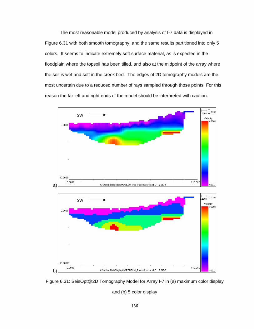
136

The most reasonable model produced by analysis of I-7 data is displayed in

Figure 6.31 with both smooth tomography, and the same results partitioned into only 5

colors. It seems to indicate extremely soft surface material, as is expected in the

floodplain where the topsoil has been tilled, and also at the midpoint of the array where

the soil is wet and soft in the creek bed. The edges of 2D tomography models are the

most uncertain due to a reduced number of rays sampled through those points. For this

reason the far left and right ends of the model should be interpreted with caution.

a)

b)

Figure 6.31: SeisOpt@2D Tomography Model for Array I-7 in (a) maximum color display

and (b) 5 color display

SW

SW

137

In order to isolate the best possible 2D tomography model, the data was also

analyzed using the generalized reciprocal method (GRM) in a program called IXRefraX

(Palmer, 1980). This software enables layer modeling and allows for horizontal variation

within the layer. It is the layer model shown in Figure 6.32 that helped to determine that

the 2D tomography model in Figures 6.30 and 6.31 provided the best result. This profile

has a much shallower bottom depth, but the first/second layer interface seems very

similar to what appears in the tomography model, especially at approximately 20-25m

from the left end.

Figure 6.32: Two-Layer Model Profile of I-7 from IXRefraX

(T. Blake, personal communication, September 11, 2012)

SW

WW

138

6.3: Comparison of Results

The models generated from a p-wave refraction survey are not directly

comparable to the Vs profile of a ReMi 2D assembly because of the difference between

P and S-wave velocities; however, they can be compared in very general and qualitative

terms for major structure or “ball-park” velocities. In both refraction models the wave

velocities fall significantly on the down-slope end of the array. This agrees with the

assembled ReMi profile, which indicates that somewhere between I-5 and I-1 there is a

significant decrease in the Vs profile through all layers. Unfortunately the trench data is

only logged to about 3m below the ground surface, and this lies entirely within the

surface layer in the geophysical models. The ReMi data seems to agree well with the

confirmed and inferred structure in Figure 4.5. Lettis and Hall (1994) show the depth of

alluvium to be much greater on the NE side of the fault trace, and this is indeed what is

indicated by the markedly lower stiffness in the 2D ReMi profile. They were also able to

confine the bedrock depth on the hanging wall to 20-30m in depth (also shown in Figure

4.5) using well log data. This is also approximately the depth that the ReMi model

shows the 1200m/s layer transition on the hanging wall.


This chapter has attained its goal of successfully measuring a significant lateral

variation in the soil stiffness profile across a fault trace. The seismic refraction data

seems extremely ambiguous, but corroborated the ReMi 2D profile. In fact, the ReMi

method seems to have shown the lateral change in stiffness more clearly than the

seismic refraction method did. Based upon the degree of uncertainty involved in each

method, it would be unwise to base conclusions on only one. Furthermore, without the

inferences made and trench data logged by experienced geologists Lettis and Hall

(1994) it would be very difficult to come to any definite conclusions about the geophysics

139

data. One must remember that the ReMi data was fit with prior knowledge from this

earlier work. Since the forward modeling process can produce such a variety of equally

well fit dispersion curves, it is a leap to say that the same can be done with no prior

knowledge. Figure 6.33 presents a summary of the results from the methods employed

in this work, as well as the trench data from Lettis and Hall (1994).

140

Figure 6.33: Summary of Model Figures and Past Trenching for Ingley Site

(trench data from Lettis and Hall (1994))

141

In the process of reaching the original goal of this chapter, a number of

interesting observations arose. These are summarized here:

Placing a ReMi array in close proximity to a strong signal source at a site that

does not receive any other similar amplitude Rayleigh waves may result in

interference (body wave or other) to the point that the p-f plots will be

uninterpretable.

The ReMi analysis is minimally affected by elevation change to the degree

present in array I-4. This array experienced grade reversal of the slope, and in

both segments the grade surpassed the 5% deviation allowance from the

SeisOpt ReMi Field Tutorial (2006)).

The spectral ratio peaks can sometimes appear much higher than the lower

bound and true phase velocities. At this site this was caused by spectral ratio

“wash out” due to a strong response along a higher phase velocity trend.

Active records can experience low frequency “wash out”, while passive records

show a much wider spread of energy along the lower bound in the mid and upper

frequency ranges. The wider spread of the spectral ratio trend causes more

uncertainty in the picking process.

At a quiet site a hammer and plate source can produce good seismic refraction

break points even in longer arrays by stacking records.

While difficult to compare the different types of data directly, watching for general

qualitative trends can help the methods to corroborate one another.

142

Chapter 7: Frontera Site Data Analysis

The Frontera Site provided an ideal location to attempt the ReMi and seismic

refraction methods in a situation where very little is known about the subsurface geology

and structure. The work consisted of eight arrays providing ReMi data at each location

and seismic refraction data at arrays M-5, M-6 and M-7. Only seven arrays are shown in

Figure 7.1, but array M-2 was also extended off the southern end of the depicted line in

order to compare results from 4 and 8m spacings.

The seismic refraction arrays lie in close proximity to the inferred fault scarp

identified during preliminary site walks. Although only array M-6 crosses this observed

feature, arrays M-5 and M-7 can provide data for comparison between ReMi and seismic

refraction results obtained through the same array set-up. Although these arrays do not

appear to cross the inferred feature, they may still indicate other structural abnormalities

in the subsurface that could indicate nearby faulting.

143

Figure 7.1: Plan of the Frontera Site Arrays with a Recent Satellite Overlay Depicting the

Geomorphic Expression Identified in the Field in the Shaded Area


In addition to the goal of imaging a fault trace with geophysical techniques, the

ReMi data at the Frontera site prompts discussion on a variety of topics that seem to

affect the p-f plot spectral ratio distributions. Throughout the site, the data showed some

strange results in nearly all ambient signal recordings. The seismographs of these

records show a considerable amount of drift during the duration of the recordings.

Possible causes for this are discussed in sections 7.1.1 and 7.1.2. The commentary on

the spectral ratio plots in this chapter includes comparisons between data collected

using different receiver spacings as well as varied source types and azimuths.

144

7.1.1: Ambient Recording Artifacts

The p-f spectral ratio plot in Figure 7.2 illustrates the common trend observed in

ambient measurements recorded throughout the site. The only clear trend in spectral

ratio peaks exists along the very top of the plot. This energy distribution indicates that

extremely rapid phase velocities are relatively constant across all frequencies. A

number of arguments lead to the belief that this is only an artifact. Velocities indicated

by these spectral ratio peaks would only be present in very stiff bedrock. The fact that

these velocities show up across the entire frequency band implies that the profile is

made up of a single layer with very high velocity. If only due to overburden confinement,

the stiffness should still increase somewhat with depth if the material in the profile is

constant. The velocities actually appear to reduce at depth based upon this plot. While

little is known about the geology of the subsurface at this site, figures obtained from

Lettis Consultants, Inc. (unpublished and not shown) conflict with this result. The figures

constrain sediment thickness and bedrock depths in the region using historical borehole

data. They clearly indicate significant alluvial deposits above bedrock, especially to the

east of the creek bed.

Figure 7.2: Example p-f Plot of Ambient Recordings Taken at Frontera Site Array M-3

145

After determining this trend to be invalid, the question yet remains as to the

cause. Interestingly, this energy distribution is much less prevalent on recordings with

actively or pseudo-actively applied sources. This suggests that, although these spectral

ratios are very high in the ambient signal plots, they are easily “washed out” whenever a

signal with significantly bigger amplitude is introduced. Additionally, in many of the

ambient plots a viable dispersion trend does exist, but along the boundary of dark blue

and purple spectral ratio regions, similar to what was shown at the Ingley site. This

implies that the energy causing this high velocity trend is strong enough to “wash out”

the dispersion trend in the ambient signal condition, but weak enough to be “washed out”

by the active or pseudo-active energy.

It is unclear what could cause this result, but four hypotheses are presented

here. Because the receivers were installed on the ground surface rather than imbedded,

it is possible that the tall grass covering the Frontera site may have been rustling against

the receivers in the wind. This should be mitigated when the wave signals are analyzed

for signal coherence during processing, but it is possible that the data was not

adequately filtered at this stage. Determining if this is truly the case would require a

higher knowledge of the algorithms built into the Optim software.

The second possibility is the noise inherent to the measurement process. When

the signal is extremely weak the noise caused by small fluctuations in the data

acquisition power source or the geophones themselves is much more significant.

Because the ReMi analysis process involves spectral ratios, at a site where the

measurement noise is close in amplitude to that of the signal it can have a significant

impact on the p-f plot.

146

The third potential cause involves the array placement. The arrays at this site

were set up nearly parallel to a large nearby road. This means that the plane wave

arrivals approaching the array will arrive approximately perpendicular to the line. If the

arrivals reach all receivers at nearly the same time, this would indicate extremely high

phase velocity regardless of frequency. This explanation would be more plausible if the

road was clearly the most energetic signal source in the area, but a highway to the south

and the nearby shopping center to the north lie almost as close. Wave front arrivals

from these sources should contain approximately the same amount of energy.

Furthermore, these arrivals would come from azimuths close to parallel with the arrays.

Although this explanation is unlikely, it cannot be completely ruled out.

The final hypothesis addressed in this work is the possibility that the high velocity

trend is an artifact of the signal drift observed in the seismograph records. This is

addressed in section 7.1.2.

7.1.2: Comparison of Filtered and Non-Filtered Drift

During data collection in the field the ambient records showed significant signal

drift during the duration of the measurements. The seismographs in Figure 7.3a exhibit

this behavior. This was not witnessed at the other sites in this research, and is likely due

to the extremely low amplitudes measured here. The Frontera site is the “quietest” of

the three sites since it is offset furthest from any road or other major signal source.

Because the amplitude scale is set automatically in VibraScope by the absolute

maximum value in the measurements, when significant signals are recorded the drift is

not noticeable. This raised the question as to how the drift may affect the data, whether

noticeable or not.

147

It seemed unlikely that this drift would affect the results because it would be

analyzed as a very low frequency wave. This frequency is far below the resonant

frequency of the geophones (4.5Hz) and would fall outside of the data range where picks

are made. In order to ensure that unforeseen effects were not being caused in the

usable data range, a low-cut filter applied at 1Hz produced the seismographs in Figure

7.3b. This filtered data was then exported and analyzed without the drift.

a)

b)

Figure 7.3: Seismographs of Ambient Signal Recorded at Array M-3 (a) with Signal Drift

and (b) Corrected for Signal Drift with the Application of a Low Cut Filter at 1Hz

148

Figure 7.4 compares the spectral ratio plots of the same data both corrected and

not corrected for drift. The only apparent difference lies in the very low frequencies

(approximately 0-3Hz) where the filtered data shows higher spectral ratios at low

slowness. This should not affect the analysis process because picks are not made at

these frequencies. Based upon this experiment, it appears that the signal drift is not

responsible for the high frequency trend at the tops of the ambient p-f plots.

a)

b)

Figure 7.4: p-f Spectra Ratio Plot of Data Processed (a) without Drift Correction and

(b) with Drift Correction

149

7.1.3: Comparison of M-2a and M-2b

At array M-2 the p-f plots from the 8m receiver spacing (M-2a) contain gaps

where the spectral ratios do not fully define the lower bound dispersion trend. For this

reason, and to compare results between differing receiver spacings, the array was

adjusted to 4m spacing. In this adjustment the northern end of the array remained in the

same location (array M-2b) and the same azimuth was maintained.

Reducing the receiver spacing should allow longer period waves to be sampled

by more receivers within a single wavelength, and thus characterize it more accurately.

Indeed, the 8m spaced array is poorly defined above approximately 8Hz. Based upon

the phase velocity picks at this frequency, the wavelength calculates as approximately

19m and therefore could be sampled by three receivers at any given moment. When the

wavelength becomes smaller than 16m, an array spaced at 8m cannot sample a single

wavelength more than twice along its length. However, a 4m spaced array could sample

wavelengths down to 8m accurately. The p-f plot of the 4m spaced array in Figure 7.5b

is well defined down to approximately a 5m wavelength. Conversely, a wavelength

longer than the entire survey line is clipped spatially. This form of aliasing may degrade

characterization of the waveform. A 12 receiver array spaced at 4m surveys 44m in

length, and this approximately matches the wavelengths at the gap in figure 7.5b around

6Hz.

150

a)

b)

Figure 7.5: p-f Spectral Ratio Plots for (a) 8m Spacing and (b) 4m Spacing at Array M-2

The picks from the 8 and 4m spaced arrays are plotted simultaneously in Figure

7.6 and show that the trends agree quite well. There is some amount of divergence

between 6 and 10Hz, but this could be attributed to lateral variation in the soil strata

since the 8m array is twice as long as the 4m array. Solid curves define the upper and

lower bounds of the picks from both arrays, and the dashed line represents a fourth

order polynomial fit to all picks from both arrays.

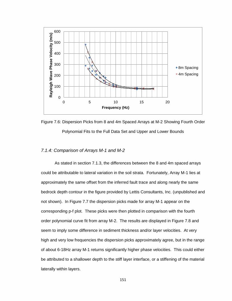
151

Figure 7.6: Dispersion Picks from 8 and 4m Spaced Arrays at M-2 Showing Fourth Order

Polynomial Fits to the Full Data Set and Upper and Lower Bounds

7.1.4: Comparison of Arrays M-1 and M-2

As stated in section 7.1.3, the differences between the 8 and 4m spaced arrays

could be attributable to lateral variation in the soil strata. Fortunately, Array M-1 lies at

approximately the same offset from the inferred fault trace and along nearly the same

bedrock depth contour in the figure provided by Lettis Consultants, Inc. (unpublished and

not shown). In Figure 7.7 the dispersion picks made for array M-1 appear on the

corresponding p-f plot. These picks were then plotted in comparison with the fourth

order polynomial curve fit from array M-2. The results are displayed in Figure 7.8 and

seem to imply some difference in sediment thickness and/or layer velocities. At very

high and very low frequencies the dispersion picks approximately agree, but in the range

of about 6-18Hz array M-1 returns significantly higher phase velocities. This could either

be attributed to a shallower depth to the stiff layer interface, or a stiffening of the material

laterally within layers.

0

100

200

300

400

500

600

0 5 10 15 20

Rayle

igh

Wav

e P

hase V

elo

cit

y (

m/s

)

Frequency (Hz)

8m Spacing

4m Spacing

152

Figure 7.7: p-f Spectral Ratio Plot Including Dispersion Picks for Array M-1

Figure 7.8: Comparison between Array M-1 Dispersion Picks and the Curve Fit to Both

Sets of Dispersion Picks at Array M-2

0

100

200

300

400

500

600

0 5 10 15 20 25

Rayle

igh

Wav

e P

hase V

elo

cit

y (

m/s

)

Frequency (Hz)

M-1

M-2 Curve Fit

153

7.1.5: Signal Source Comparison

This section focuses on comparing spectral ratio p-f plots obtained through

measurement of various signal types at different azimuths. Arrays M-3 through M-7

provided some interesting data that indicated multiple response trends characteristic of

Rayleigh wave dispersion. Active records at arrays M-6 and M-7 also show some very

irregular response distributions that warrant discussion.

7.1.5.1: Active Source Comparison

Array M-3 produced two very different energy response trends shown in the p-f

plots of Figures 7.9 and 7.10. The two signal conditions presented are actively

generated by walking vibrations and hammer blows respectively. At first glance the

trend exhibited in Figure 7.9a seems to be the clear dispersion trend for array M-3.

However, when the walking signal data is compared to the off-end hammer data of

Figure 7.10 the true dispersion trend is unclear. The dataset collected with the hammer

energy presents a lower phase velocity trend in addition to that found in the walking

signal records. If the walking records are interpreted with knowledge of this lower

trend’s existence, similar picks can be made along the blue-to-purple boundary. Picks

for both trends are displayed for the walking and hammer signal records in Figures 7.9

and 7.10.

154

a)

b)

Figure 7.9: p-f Spectral Ratio Plots of Walking Induced Signal at Array M-3 with

Dispersion Picks along the (a) Upper Trend and (b) Lower Trend

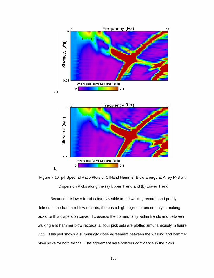
155

a)

b)

Figure 7.10: p-f Spectral Ratio Plots of Off-End Hammer Blow Energy at Array M-3 with

Dispersion Picks along the (a) Upper Trend and (b) Lower Trend

Because the lower trend is barely visible in the walking records and poorly

defined in the hammer blow records, there is a high degree of uncertainty in making

picks for this dispersion curve. To assess the commonality within trends and between

walking and hammer blow records, all four pick sets are plotted simultaneously in figure

7.11. This plot shows a surprisingly close agreement between the walking and hammer

blow picks for both trends. The agreement here bolsters confidence in the picks.

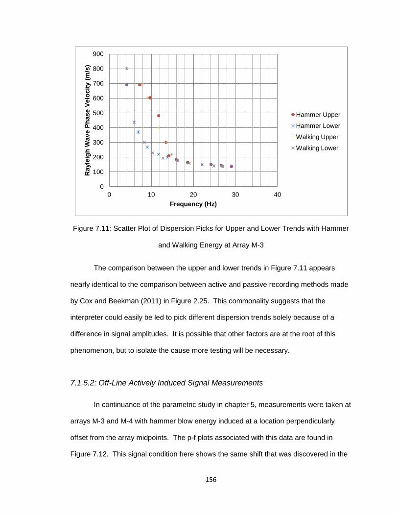
156

Figure 7.11: Scatter Plot of Dispersion Picks for Upper and Lower Trends with Hammer

and Walking Energy at Array M-3

The comparison between the upper and lower trends in Figure 7.11 appears

nearly identical to the comparison between active and passive recording methods made

by Cox and Beekman (2011) in Figure 2.25. This commonality suggests that the

interpreter could easily be led to pick different dispersion trends solely because of a

difference in signal amplitudes. It is possible that other factors are at the root of this

phenomenon, but to isolate the cause more testing will be necessary.

7.1.5.2: Off-Line Actively Induced Signal Measurements

In continuance of the parametric study in chapter 5, measurements were taken at

arrays M-3 and M-4 with hammer blow energy induced at a location perpendicularly

offset from the array midpoints. The p-f plots associated with this data are found in

Figure 7.12. This signal condition here shows the same shift that was discovered in the

0

100

200

300

400

500

600

700

800

900

0 10 20 30 40

Rayle

igh

Wav

e P

hase V

elo

cit

y (

m/s

)

Frequency (Hz)

Hammer Upper

Hammer Lower

Walking Upper

Walking Lower

157

Crops Field C-31 analysis. The spectral ratio peaks appear higher on the p-f plot,

indicating higher phase velocities. Again, this is likely due to the fact that the arrivals

from a source off-line from the array midpoint will reach all receivers in more rapid

succession than if traveling along the length of the array (see Figure 5.11).

This data also provides a new insight that was not so clearly observable in the

Crops Field C-31 data. In examination of the p-f plots in Figure 7.12, there appear to be

a number of trends indicating higher spectral ratios moving from the bottom left of the

plot up and towards the top-right corner. These irregular trends pass through the

Rayleigh wave dispersion zone of the plot and cause significant interference with the

dispersion curve where they meet. This makes the lower bound very difficult to identify.

The cause for these elevated spectral ratio curves is unclear, but the subject is moot

because the dispersion trend is unreliable in this signal condition. The information

presented here should only be used to help an interpreter recognize the effects and

avoid using records exhibiting this behavior.

158

a)

b)

Figure 7.12: p-f Spectral Ratio Plot of Hammer Energy Originating at a Location

Perpendicularly Offset from the Midpoint of Array (a) M-3 and (b) M-4

159

7.1.5.3: Differences Observed between In-Line Active Energy Produced Off of

Opposite Array Ends

At array M-5 the dispersion trend in the p-f plots shows very good definition

throughout records containing actively or pseudo-actively induced energy. Although well

defined, the trends seem to diverge from one another in the frequency range above

approximately 30Hz. Recordings of hammer blows off the NW end of the array differ

from those of hammer blows off the SE end. Figure 7.13 displays the plots and picks for

these two conditions. The difference between these plots is likely due to lateral variation

in the soils strata. When hammer blows are recorded off-end of the array, the respective

end of the line receives a much stronger signal and may therefore more clearly reflect

the profile under those receivers. If this is the case, the signal seems to attenuate

rapidly enough that the dispersion at the other end of the array is “washed out”. This

effect could be mitigated by increasing the source-array offset so that the ratio of the

amplitudes observed at opposite ends is smaller.

160

a)

b)

Figure 7.13: p-f Spectral Ratio Plots for Array M-5 Containing Off-End Hammer Energy

from (a) the SE and (b) the NW

7.1.5.4: Irregular Spectral Power Distributions

The p-f plots for Arrays M-6 and M-7 contain scattered zones with elevated

spectral ratios. This strange behavior may be a result of the proximity to the inferred

fault trace. Array M-6 actually crosses the inferred fault scarp and M-7 rests just atop

the inferred hanging wall. Each of the wave field cases described in this section

returned considerably different dispersion trends, or at times, no clear trend whatsoever.

161

Because the trends vary so drastically, no picks were made for array M-6. In this case

dispersion picks would be meaningless because the array crosses the inferred fault

trace. Modeling an array crossing a fault offset would not help to characterize the fault

since it would just smear the results across the array.

The data containing hammer blows off-end of array M-6 is presented in Figure

7.14 and indicates a high level of variance across the array. The two ends of the array

do not appear to agree with one another, even in an approximate sense. Despite the

disagreement, a commonality does exist. Many small zones with elevated spectral

ratios appear in both plots above approximately 25Hz. These zones are uncharacteristic

of typical p-f plots even above the frequencies where the dispersion trend is clearly

defined. Figure 7.15 displays very similar data recorded at array M-7. This could

potentially be caused by some complicated subsurface structural geometry that is

resulting in ray scatter through diffraction, refraction, and reflection. If this is the case,

this abnormal distribution of spectral ratio peaks could potentially indicate that the fault

trace exists beneath the array and is responsible for the anomalous data.

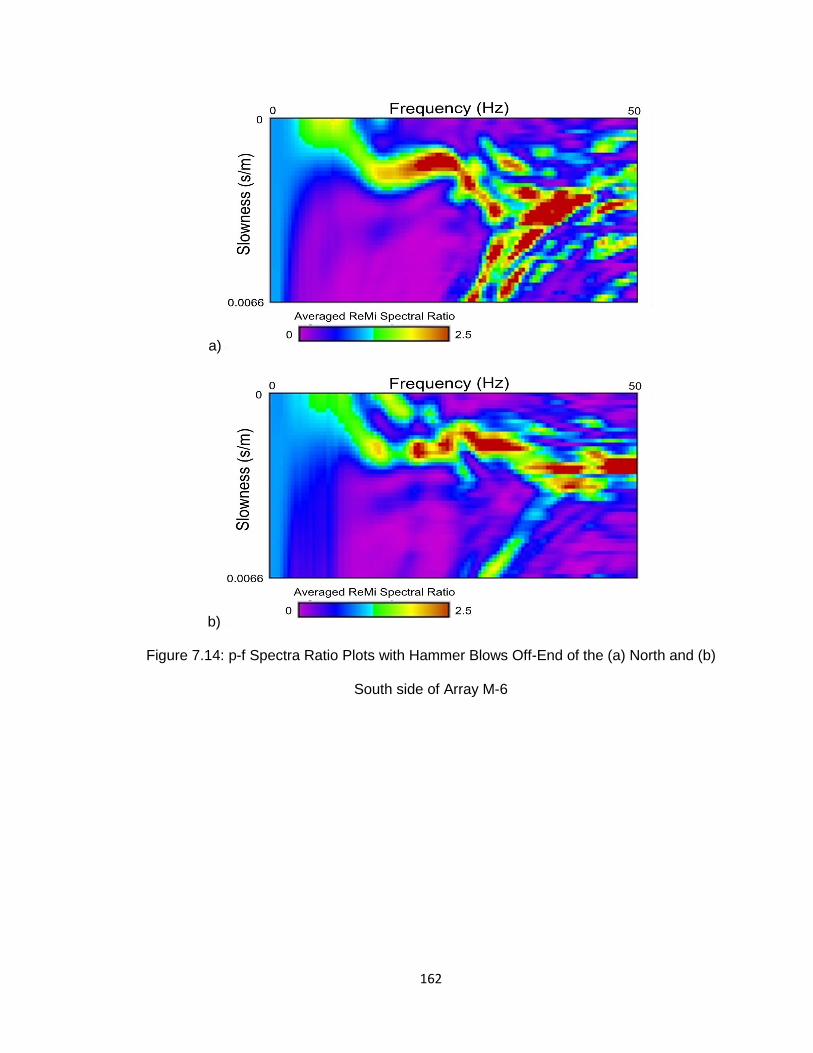
162

a)

b)

Figure 7.14: p-f Spectra Ratio Plots with Hammer Blows Off-End of the (a) North and (b)

South side of Array M-6

163

a)

b)

Figure 7.15: p-f Spectra Ratio Plots with Hammer Blows Off-End of the (a) South and (b)

North sides of Array M-6

7.1.6: Forward Modeling and 2D Profile Assemblies

The analysis of the data collected at the Ingley site revealed that ambiguity in the

modeling process introduces far more uncertainty than decisions made during the

dispersion picking process. Because this is the case, rather than making bracketed

picks for each p-f plot, at each array all the picks made for the varied cases were

combined to guide the forward modeling process. Figures showing theoretical

dispersion curve fits to the experimental picks can be found in the appendix of this work.

For brevity’s sake only the final models are included here in the body of the report.

164

The figures provided by Lettis Consultants, Inc. (unpublished and not shown)

provided some valuable aid during the forward modeling process. Using the sediment

thickness and bedrock depth information, possible model fits for the picks at array M-2

were fairly well constrained. The top layer velocity is the most easily determined since it

does not rely upon the lower layers or layer interfaces. Therefore, with the top layer

velocity and bedrock depth determined, the model in Figure 7.16 provides the best fit.

The first layer interface and lower layer velocities could be adjusted slightly, but as

determined in the Ingley analysis, the ReMi modeling process can only be relied upon

for bulk approximations. The uncertainty has been constrained as much as possible

here.

Figure 7.16: 1D Model Profile for Array M-2

Where possible, the other arrays were modeled by setting layer velocities to

approximately the same values as determined at array M-2. This constrained interface

depths and produced the models in Figures 7.17 and 7.18. The top layer velocities were

forced to increase somewhat by the experimental data as the arrays stepped closer to

the fault trace, but based upon field observations this increase in stiffness seems

appropriate. Arrays M-1 and M-2 were situated on very soft and moist topsoil, while the

arrays closer to the fault were placed on clearly dryer and stiffer material.

165



Fitting array M-7 to the same layer velocities as the other models proved to be

impossible. The entire profile showed a marked increase in stiffness similar to the

hanging wall at the Ingley site. This increase in stiffness is the anticipated shift that

indicates the possibility of a fault offset.


In order to better illustrate the degree that the overall profile stiffness changes

across the Frontera site, Figure 7.20 displays the complete 2D profile assembly. It is

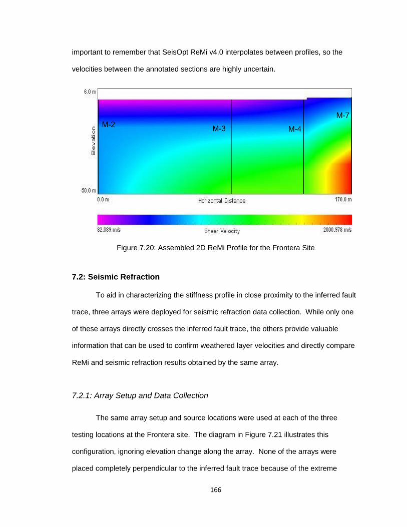
166

important to remember that SeisOpt ReMi v4.0 interpolates between profiles, so the

velocities between the annotated sections are highly uncertain.

Figure 7.20: Assembled 2D ReMi Profile for the Frontera Site


To aid in characterizing the stiffness profile in close proximity to the inferred fault

trace, three arrays were deployed for seismic refraction data collection. While only one

of these arrays directly crosses the inferred fault trace, the others provide valuable

information that can be used to confirm weathered layer velocities and directly compare

ReMi and seismic refraction results obtained by the same array.

7.2.1: Array Setup and Data Collection

The same array setup and source locations were used at each of the three

testing locations at the Frontera site. The diagram in Figure 7.21 illustrates this

configuration, ignoring elevation change along the array. None of the arrays were

placed completely perpendicular to the inferred fault trace because of the extreme

167

elevation change that would have to be traversed. The slope is dramatic enough that it

would be necessary to survey horizontal receiver offsets as well as elevation change to

obtain reliable results. This would prove problematic without a survey grade GPS unit or

total station. Instead, array M-6 was situated such that the survey obliquely crosses the

inferred fault trace with minimal elevation change. Although the vertical deviation was

reduced by taking this approach, the receiver elevations were still approximated using a

surveying tape and hand held sight level.

Figure 7.21: Diagram of Frontera Seismic Refraction Arrays

7.2.2: First Break Picking

The seismographs for all three arrays at the Frontera site suggest a significant

amount of ray scatter in the records. Due to a combination of refracted, reflected and

diffracted wave arrivals, the recordings show some very convoluted signals after the

initial arrivals. This is especially visible in Figure 7.22 where the records become highly

erratic. While filtering can help to remove some of the incoherent noise, it also tends to

cause slight shifts in the first break point arrivals. Therefore, it is more accurate to make

picks without filtering when possible. Rather than filtering all channels, approximate

picks were made on traces with bad signal to noise ratios. Picks made from filtered data

would likely be equally uncertain.

168

The picking process for array M-5 proved problematic due to some confusion in

the first arrivals. This could be in part due to the ray scatter effect that was discussed in

the previous paragraph. One end of the array lies near the creek bed where deposited

cobbles and boulders could cause rays to take complicated paths. At approximately the

array midpoint lies an erosion channel that appears to have similar deposits.

Fortunately, the off-end shots provided clearer arrivals. An example of the

seismographs and associated first break point picks of an off-end source record is

shown in Figure 7.23. This array was modeled using only off-end data.

Figure 7.22: Seismic Refraction Record for Array M-5 with Source Located between

Receivers 4 and 5

169

Figure 7.23: Seismic Refraction Record for Array M-5 with Source Located

8m Off-End of Receiver 1

Fortunately, Arrays M-6 and M-7 showed better first break point arrivals for all

source locations. They too exhibit some erratic behavior later in the recordings, but the

first break points are well defined. Examples of the stacked records and associated

picks appear in Figures 7.24 and 7.25.


between Receivers 3 and 4

170


between Receivers 2 and 3

7.2.3: Model Profiles

This section discusses the 2D tomography and layer models generated from the

seismic refraction data in [email protected] and IXRefraX. Again, all Optim plots in this

work are in distance units of meters and P-wave velocity units of meters per second.

The seismic refraction models are also compared with results obtained through the ReMi

method, and array M-7 provides a number of possible model fits from SeisOpt that

demonstrate the uncertainty involved in the forward modeling process.

The 2D tomography models presented here have been chosen based upon RMS

error from the fit of theoretical travel time curves to the experimental data, “hitfiles” ray

coverage plots like the one in section 6.2.3, inferred knowledge about the local geology,

and agreement with the layer models output from IXRefraX.

171

7.2.3.1: M-5 Models

The plots in Figure 7.26 provide the 2D tomography model determined the most

appropriate for array M-5. The depth to the first layer interface approximated by the

green/pink boundary in Figure 7.26b agrees closely with the layer interface of the

IXRefraX layer model depicted in Figure 7.27. The P-wave velocities also appear to

agree, increasing confidence in the model.

a)

b)

Figure 7.26: 2D Tomography of Array M-5 Data with (a) 257 Colors and (b) 3 Colors

NW

NW

172

Figure 7.27: Layer Model of Array M-5 Data Output from IXRefraX


The 1D ReMi model for this array shown in Figure 7.38 does not agree well with

the seismic refraction data. The velocities in the surface layer seem to be consistent if

the S-wave velocity is approximated as 2/3 the P-wave velocity, but the layer depth at

the first interface is far deeper in the ReMi model. The deeper layer velocities are also

much higher in the seismic refraction models. This could be explained by the fact that

the lower portion of the 2D tomography is very unreliable due to limited ray coverage.

Based upon the frequency and phase velocity of the picks that define the top layer in the

ReMi model, the wavelengths being measured sample a minimum depth of about 5m.

This is already below the layer interface suggested by the seismic refraction models.

The data indicates that, for very near surface measurements, the ReMi method needs

data at higher frequencies than are easily generated in the field.

NW

173

The bottom layer of the ReMi model agrees with the velocity of the bottom layer

in the seismic refraction layer model, as well as the 2D tomography model, but the depth

to that layer is in disagreement by as much as 30m. It is unclear why there is such a

gross difference between methods here. More testing is necessary to determine what is

causing the discrepancy.


7.2.3.2: M-6 Models

The models generated by SeisOpt and IXRefraX are included here in Figures

7.29 and 7.30. The IXRefraX models clip the ends of the survey where ray coverage is

limited, and the 2D tomography model only provides approximate inferences. Along the

middle of the survey the models seem to agree insofar as the depth to the first layer

interface and the general geometry of that interface. For instance, both models indicate

a bulge in the layer interface at approximately 15m from the north end of the plot. The

velocities in the top layer also seem to be in general agreement with one another. There

is no ReMi model to compare with these results due to the uncertainty in the generated

p-f plots and the fact that the array crosses the inferred fault trace.

174

a)

b)

Figure 7.29: 2D Tomography of Array M-6 Data with (a) 257 Colors and (b) 3 Colors

N

N

175



7.2.3.3: M-7 Models and Demonstration of Modeling Uncertainty

Occasionally, after eliminating the obviously erroneous 2D tomography models

there are still a number that seem to be equally valid. This is where using another

modeling program such as IXRefraX can help further isolate the best profile. If other

software is not available, or the results do not adequately support any given model, it

can be very difficult to decide which is more accurate. To demonstrate this modeling

uncertainty, a few of the SeisOpt outputs with varying resolution are included on the

following pages. All were generated using the same data set and agree fairly well with

the IXRefraX layer model.

N

176

a)

b)

Figure 7.31: 2D Tomography Model Output from SeisOpt for Array M-7 with

(a) 257 Colors and (b) 5 Colors

N

N

177

a)

b)



N

N

178

a)

b)



N

N

179


(T. Blake, Personal Communication, September 11, 2012)

It’s possible that different 2D tomography software such as Rayfract may provide

a better comparison with SeisOpt better help to determine which model is most accurate.

Unfortunately, this study was confined to the modeling software presented herein. The

layer models output by IXRefraX do not include information to nearly as great of depths

as the output from SeisOpt. Given that ray coverage is worse near the bottoms of the

SeisOpt models and there is no other software to compare with at these depths, any

interpretations here should be made with extreme caution.

In comparison with the ReMi 1D model, the methods again show extreme

disagreement. The refraction models seem more appropriate given the visible

geomorphology at the site. There appear to be bedrock outcrops very near to array M-7,

N

180

yet the ReMi method shows softer (about 450m/s) deposits all the way down to

approximately 14m. While this interface depth is uncertain, the method should be able

to locate the interface to better than 11m accuracy (the difference between stiff layer

interfaces of the two methods). Ultimately, it is impossible to know for certain which test

is more accurate without further investigation.



This chapter partially met its goal to locate a blind fault trace using the seismic

refraction and ReMi methods with little supporting information. The ReMi data

throughout the site indicates a marked increase in stiffness laterally as the inferred fault

trace is approached and traversed. This finding gives some hope that further research

may develop the ReMi method into a useful tool to aid in fault mapping. Unfortunately,

the seismic refraction models did not provide much added insight into the fault location

or geometry.

During the analysis of the data in this chapter a number of important

observations came to light that provide topics for further research and may aid future

work.

181

ReMi data collected at quiet locations such as the Frontera site can indicate false

dispersion trends due to “wash out” of the true Rayleigh wave dispersion. This

might be caused by vegetation contacting the receivers, noise inherent to the

measurement equipment, or the presence of a dominant signal source coming

from an azimuth out of line with the receivers.

Signal drift through the course of a ReMi recording can be ignored because it is

processed as a low enough frequency that it does not affect the range of data

where dispersion picks are made.

The data collected at this site seems to suggest that by adjusting the receiver

spacing and array length such that it can sample a given wavelength at three

locations simultaneously may improve the data.

Close proximity energy sources offset perpendicularly from the midpoint of the

array can produce a high density of elevated spectral ratio curves moving from

bottom left to top right of the p-f plots.

Close proximity energy sources arriving in line with the array from one end can

produce significantly different results than when approaching from the opposite

end. This may be due to lateral variation in the soil strata beneath the array in

conjunction with “wash out” of the data caused by significantly higher energy

arrivals at the near end.

Abnormal distributions of spectral ratio peak zones in the p-f plots such as those

generated from arrays M-6 and M-7 may indicate abnormal subsurface structural

geometry. This could potentially indicate the presence of a fault and can easily

be tested further to determine if this is a consistent result in the presence of such

a feature.

182

Erratic seismic refraction recordings may indicate a high degree of ray scatter

from diffraction, reflection and refraction. This could again indicate abnormal

subsurface structural geometries and potentially a fault.

The ReMi and seismic refraction methods showed extreme disagreement in this

chapter. A more controlled comparison between methods is warranted before

the two should be further used together for fault mapping.

183

Chapter 8: Conclusions and Recommendations

8.1: Summary

Locating blind fault traces can be a time consuming and costly process using

typical borehole or trenching investigation techniques. At the same time, it is a crucial

part of the design process and is often times a determining factor in whether or not a

project is feasible in a given location. In the cases of large infrastructure such as

highways or rail lines it is impossible to avoid crossing active fault traces at some point,

but knowledge of the location where displacements may occur can help engineers

mitigate the risk as much as possible. This body of work investigated the potential of the

non-invasive seismic refraction and ReMi methods as tools to aid in locating these

elusive fault traces.

In the process of achieving the primary goal of this thesis a number of parametric

and precision studies were carried out in order to better understand the ReMi method.

In addition, this work contains novice observations made while learning to use both the

ReMi and seismic refraction methods. Although experienced geophysicists may find

some of this information obvious, it is the hope of the author that this body of work can

serve as a guide to students or other newcomers who wish to be able to contribute to the

topic.

After developing a workable understanding of the theory and practice involved

with the ReMi and seismic refraction methods, the techniques are applied to the goal of

successfully imaging lateral variation in the soil strata. A dramatic change in the soil

stiffness profile over a short horizontal distance could indicate the presence of a reverse

or normal fault. This research first attempts the methods at a location where the fault

184

trace has been thoroughly investigated through trenching and drilling, then proceeds to a

site with very little available subsurface information

The ReMi and seismic refraction methods require relatively minimal time and

cost, and can be employed entirely at the ground surface. This research showed

promise that these techniques may through further development and testing provide a

means to rapidly isolate the location where a blind fault trace likely exists. However,

based upon the levels of uncertainty here observed within these methods, it is unlikely

that they will ever be reliable enough to completely replace traditional trenching or

borehole investigations.

The subsequent sections of this chapter present the primary findings of this

project, suggest improvements to the testing procedures, and offer opportunities for

future research.

8.2: Research Findings

This project produced a number of important findings that are summarized in this

section. In addition to the larger goal of applying the ReMi and seismic refraction

methods to fault mapping, the parametric, sensitivity and precision studies carried out in

this work provided some valuable insight into the intricacies of the ReMi method. A

number of key observations made along the way are also presented.

The precision study carried out at Crops Field C-31 helped to characterize the

uncertainty that can be expected within the ReMi method when all controllable variables

are held constant. Results indicate a 7% COV in Vs30, and as high as 14 and 16% in

layer interfaces and velocities respectively. This dataset also suggests that at larger

185

depths and/or higher phase velocities the method becomes more stable. At the bottom

layer of the models in this study only an 8% COV was found in Vs.

Parametric studies on the ReMi method at both Crops Field C-31 and the

Frontera site indicated that, when a dominant off-line source is introduced to the wave

field, the dispersion trend in the p-f plots will shift to higher phase velocities due to the

obliquity of the wave front arrivals with respect to the array. The response at the true

phase velocities is “washed out” here due to the strength of active signal used for this

study.

A sensitivity study at the Ingley site helped to evaluate the effect that relative

elevation change between receivers can have on the ReMi method. Slope corrected

and non-corrected results appear nearly identical at array I-4. This array traversed

grades sometimes steeper than 6.7% without adversely affecting the measurements.

Throughout this work the passive ReMi measurements exhibited weakly lit

dispersion trends or uninterpretable data. The list of potential causes for this is provided

below, but not all of these hypotheses apply to every array.

1. Significant lateral variation in the subsurface beneath the array, causing the

spectral ratio peak trend to be more widely distributed and less sharply defined

2. Body wave interference generated by close proximity utility lines

3. Body wave interference from a nearby dominant signal source

4. Nearby slopes acting as a discontinuity in the soil strata thereby affecting wave

propagation

5. Vegetation contact with receivers

6. Noise inherent to the measurement equipment

186

With respect to the primary goals of this work, these methods do show potential

for future development. In particular, the 2D assemblies of 1D ReMi profiles indicated

marked lateral variation in the Vs profiles at both the Ingley and Frontera sites. While

this bulk shift can be trusted in a very general sense, the data is too uncertain to rely

upon quantitatively. It should also be noted that the layer velocities do not agree

quantitatively between methods.

The final ReMi models from the Ingley site arrays also showed general

agreement with the work by Lettis and Hall (1994). These models were not constructed

through a blind analysis, but fitting them to the available subsurface data was not

difficult. The theoretical dispersion curves that characterize the modeled profiles fit the

data as closely as if no attempt were made to match the available information.

At the Frontera site the 2D assembled ReMi model qualitatively matches the

observed geomorphology. While the method does not definitively prove that the inferred

scarp feature is a fault, it does vindicate the suspicion that was previously based solely

upon the site topography. Despite the uncertainty in the ReMi method, this could

potentially become a litmus test as to whether or not further investigation is warranted at

a given location.

The seismic refraction results did not as clearly indicate any evidence of faulting.

At the Ingley site the layer and tomography models helped to corroborate general

interface depths and velocities found in the ReMi testing, but at the Frontera site the

methods showed complete disagreement. To further employ the seismic refraction

method in conjunction with the ReMi method for fault mapping, the two should be first

successfully matched in a more controlled situation.

187

The final and possibly most important finding of this work is in the irregularity of

data collected in close proximity to the known and inferred fault traces. Both the ReMi

and seismic refraction data displayed odd behavior in the p-f plots and seismographs

respectively. When plotted in p-f space, the ReMi data exhibited abnormally distributed

energy. Many spectral ratio peak zones appeared above the general dispersion trend.

While the exact cause for this phenomenon is unclear, the consistency of this

occurrence among records taken in close proximity to the fault should not be ignored.

Similarly, the seismographs for the seismic refraction data became very erratic in the

arrays near the inferred fault trace at the Frontera site. The anomalous behavior of both

methods may possibly be attributed to abnormalities in the subsurface structure caused

by faulting.

8.3: Improvements on Testing Methods

To aid future researchers in better planning their geophysical surveys, this

section provides a number of suggestions that may help enhance data collection and

lead to better results.

For the ReMi method:

1. Arrays should be spaced such that the wavelengths of interest are most

effectively measured. If a given wavelength can be measured simultaneously at

three or more points spread out along the full length, it will be more accurately

characterized.

188

2. If a wide variety of wavelengths are of interest multiple array spacings can be

deployed with the same survey midpoint. Picks that are made independently

from each array can be combined manually for forward modeling.

3. Underground utility lines and nearby dominant signal sources should be avoided

to minimize record contamination by body waves.

4. If a majority of the ambient signal is coming from a known direction it is helpful to

orient the array such that the arrivals will be traveling parallel to the array

azimuth.

For the seismic refraction method:

1. Overlapping multiple arrays with smaller receiver spacing is preferable to using a

single array if time warrants. This can greatly improve imaging resolution and

signal strength.

2. If available, a more energetic source is helpful.

3. A smaller data acquisition time step (0.125ms) makes first break picking easier.

4. If available, survey equipment can help to greatly reduce the uncertainty caused

by receiver location input error.

8.4: Opportunities for Further Investigation

A number of opportunities for future research were uncovered during this project.

While not within the scope of work for this dissertation, the following list provides future

researchers with some potential avenues for investigation.

The precision study within this body of work could be built upon with much larger

datasets. Three suites of testing are not an adequate dataset to make reliable

189

statistical conclusions. It would be easy to take a large quantity of data for this

purpose in a single day.

As mentioned in section 8.2, the ReMi and seismic refraction methods generally

did not quantitatively agree in this research. If the two are ever to be used in

conjunction with one another, the analysis techniques need to first be calibrated

so that the methods agree in a controlled situation. Only then can they be

trusted in their agreement in more complex scenarios.

Further testing at the sites investigated in this work could help to isolate the

cause(s) of the poor results obtained through passive measurements. The list of

hypotheses summarized in section 8.2 provides a good starting point for this

endeavor.

A method for determining measurement noise levels and thus the required signal

amplitude to collect good passive data would aid future researchers in

determining when a site is too quiet for the ReMi method.

Further data collection from either method in close proximity to reverse or normal

fault traces may help to either corroborate or disprove the hypothesis that the

irregular data collected in this work resulted from fault-related subsurface

structure.

190

References

Aki, K. (1957). “Space and time spectra of stationary stochastic waves, with special

reference to microtremors.” Bull. of the Earthquake Res. Inst., University of Tokyo, 12(5),

415-456.

American Society for Testing and Materials (ASTM). (2006), "Standard guide for using

the seismic refraction method for subsurface investigation." D 5777, West

Conshohocken, PA.

American Society for Testing and Materials (ASTM). (2007), " Standard test methods for

crosshole seismic testing." D 4428, West Conshohocken, PA.

American Society for Testing and Materials (ASTM). (2008), " Standard test methods for

downhole seismic testing." D 7400, West Conshohocken, PA.

Cox, B.R. and Beekman, A.N. (2011). “Intramethod variability in ReMi dispersion

measurements and Vs estimates at shallow bedrock sites.” J. Geotech. and Geoenv.

Eng., 137(4), 354-362.

Jones, R.B. (1958). “In-situ measurement of dynamic properties of soil by vibration

methods.” Geotechnique, 8(1), 1-21.

Kitsunezaki, C. (1975). “Shear wave logging by suspension type geophone, I.” Butsuri-

tanko, 28, 13-21.

Lay, T. and Wallace, T. C. (1995). “Modern Global Seismology.” Academic Press,

San Diego, CA.

Lettis, W. and Hall, T. (1994). "Los Osos fault zone, San Luis Obispo county,

California." Special Paper – Geol. Soc. of Amer., 292, 73-102.

Louie, J. N. (2001). “Faster, better: shear wave velocity to 100 meters depth from

refraction microtremor arrays.” Bull. Seismol. Soc. Am., 91(2), 347-364.

McMechan, G. and Yedlin, M. (1981). "Analysis of dispersive waves by field

transformation." Geophysics, 46(6), 869-874.

191

Moss, R. E. S. (2008). “Quantifying measurement uncertainty of thirty-meter shear-wave

velocity.” Bull. Seismol. Soc. Am., 98(3), 1399-1411.

Nazarian, S. and Stokoe, K . H. (1984). "In situ shear wave velocities from spectral

analysis of surface waves." Proc., Eighth World Conf. on Earthquake Eng., Prentice-Hall,

Inc., Englewood Cliffs, Nj., 3, 1-38.

Ohya, S., Ogura, K., and Imai, T. (1980). "The suspension PS velocity logging

system." Proc., Offshore Technology Conference, Offshore Technology Conference,

Houston, Tx., 1, 291-298.

Palmer, D. (1980). “The Generalized Reciprocal Method of Seismic Refraction

Interpretation.” Soc. of Exploration Geophysicists., Tulsa, OK.

Parasnis, D. S. (1986). “Principles of Applied Geophysics”. Chapman and Hall,

Boundary Row, London, UK.

Park, C. B., Miller, R. D., and Xia, J. B. (1998). "Imaging dispersion curves of surface

waves on multi-channel record." Proc. SEG Annual Meeting, Soc. of Exploration

Geophysicists, New Orleans, LA.

Park, C. B., Miller, R. D., and Xia, J. B. (1999). "Multichannel analysis of surface

waves." Geophysics, 64(3), 800-808.

Park, C. B., Miller, R. D., Ivanov, J., Xia, J. B., and Ryden, N. (2005). "Combined use of

active and passive surface waves." J. Env. and Eng. Geophys., 10(3), 323-334.

Pérez-Santisteban, I., García-Mayordomo, J., Martín, A. M., and Carbó, A. (2011).

“Comparison among SASW, ReMI and PS-logging techniques: Application to a railway

embankment.” J. Applied Geophys., 73(1), 59-64.

Redpath, B. B. (1973). “Seismic refraction exploration for engineering site

investigations.” Army Engineer Waterways Experiment Station, Livermore, CA.

Thorson, J. R. and Claerbout, J. F. (1985). "Velocity-stack and slant-stack stochastic

inversion." Geophysics, 50(12), 2727-2741.

192

Tokimatsu, K., Shinzawa, K., and Kuwayama, S. (1992). “Use of short-period

microtremors for Vs profiling.” J. of Geotech. Eng., 118(10), 1544-1558.

Yuan, J. ( 011). “Field studies comparing SASW, Beamforming and MASW test

methods and characterization of geotechnical materials based on Vs.” Doctoral

dissertation, University of Texas, Austin, TX.

fault mapping with the refraction microtremor and seismic

Documents