fault detection and localization using continuous wavelet transform...
TRANSCRIPT

International Journal on Electrical Engineering and Informatics - Volume 10, Number 2, June 2018
Fault Detection and Localization using Continuous Wavelet Transform
and Artificial Neural Network Based Approach in Distribution System
Himadri Lala1, Subrata Karmakar1 and Sanjib Ganguly2
1Department of Electrical Engineering, NIT Rourkela, Rourkela, Odisha-769008, India
2Department of Electronics and Electrical Engineering, IIT Guwahati, Assam-781039, India
Abstract: This article presents an advanced continuous wavelet transform (CWT) based
approach for fault detection and localization in distribution systems using the artificial neural
network (ANN). In this study, CWT extracts distinct features from the transient signals
captured from the bus. The derived features are utilized to train and test appropriate ANN
architecture in different stages to detect and localize the faults. The proposed scheme
provides an optimum method for classification as well as localization of the various kinds of
fault with different source short circuit (SSC) level in different locations. The whole detection
and localization process consists of several stages. In the first stage, it detects faulty feeder.
The faulty line is identified in the second stage. Finally, in the third stage, fault type and fault
location are being calculated from the relaying point. The performance of the proposed CWT-
ANN based approach is quite promising as compared to traditionally used algorithms.
However, a correlation-based feature selection technique is also implemented to reduce
training time and improve accuracy. This algorithm is tested in 11 kV radial Indian
distribution network but can be applied in other distribution networks also.
Keywords: Continuous Wavelet Transform, Artificial Neural Network, Fault localization,
Fault Detection, Unsymmetrical fault, Distribution system.
1. Introduction
The rapidly growing demand for electric power leads to interconnection in power systems.
With the increasing number of interconnections between power systems, it becomes more and
more complicated [1]. The most important role of all the power system engineers is to ensure
utmost reliability and continuity of service. It is also essential to reduce the repair time and speed
up the system restoration after a fault. The outage time of power increases due to old fault
detection and localization techniques [2]–[6]. It causes massive workforce and time wastage.
Although there are few types of equipment exist in the substations, which designed to detect and
localize the faults, do not always give an accurate result. Therefore, it is highly needed to identify
the faults and its exact location, so that system restoration process becomes faster. It is not
feasible to avoid the natural hazards, accidents, and dis-operation of power system equipment.
The fault causes transients in distribution systems, which are not easy to identify because of their
short duration. The instrument for measuring the transient are ought to have a high sampling rate
to give accurate precision in portraying transient conditions concerning their amplitude and
frequency content. These qualities are fundamental for performing a transient investigation.
In the power system literature, CWT based approaches are applied to detect and localize
faults in the past [2]. However, there are different other methodologies for investigating power
system transients. The expert systems [7], fuzzy based systems [8], various optimization
techniques [9], ANN [10], different wavelet transform methods [11], etc, are the various
favourite techniques. All of the above methodologies suffer from higher computational time,
lack of robustness and accuracy in performance. Unlike Discrete wavelet transform (DWT) few
researchers applied CWT [12] for detection [13] of distribution system faults. The CWT is one
of the most useful techniques in analyzing system transients along with soft computing
Received: March 27th, 2018. Accepted: June 23rd, 2018
DOI: 10.15676/ijeei.2018.10.2.1
203

technologies. In [3] D. Thukaram et al. proposed a fault detection and localization technique
using principle component analysis (PCA) as an extractor of distinct attributes and support vector
machine (SVM) and ANN as the classifier and estimation tool. This method is an impedance-
based method. The error in location estimation is nearly around 10 m. In the past several years,
different researchers have proposed various fault-location estimation techniques. Mirzaei et al.
[14] and Mora et al. [15] Saha et al. [16] reviewed different methods of localizing faults such as
impedance-based, frequency, and knowledge-based methods. According to Mirzaei et al., high-
frequency based method along with knowledge-based methods gives a much accurate result in
fault localization. In continuation of previous literature, Yadav et al. [17] applied DWT and ANN
to localize fault in double circuit transmission line. It gives accuracy, which is not much higher
in some cases, and in the distribution network, this algorithm is not tested. In the [18], Saleh et
al. implemented a DWT based dynamic voltage restorer in a distribution system. Whereas,
Samantaray et al. proposed combined H-S transform and ANN based fault localizer [19] in
power transmission system. As in distribution network, previous localization results are lesser
accurate, or the methods of estimation are complex which results in increasing calculation or
computational time and indeed increases the complexity of the system. Zhang et al. suggested a
discernible signal analysis for distribution system [20] ground faults, but the main shortcoming
of the scheme is that it cannot eliminate the consequences of high impedance fault. Yong et al.
Proposed a DWT based method to identify the type of fault in the distribution system [21].
However, Lovisolo et al. have attempted to detect and localize the fault which causes voltage
sag and swell [22]. The results provide accurate detection of the fault, but it gives relatively low
fault localization accuracy (85%). In [23] a CWT-ANN based detection and localization
algorithm is applied on a hybrid distributed generation systems. The results regarding fault
localization are encouraging, but it needs to be optimized and implemented in a distribution
system. The overall scenario of fault detection and localization algorithm stands on two basic
pillars, i.e. signal processing and soft computing techniques. The various signal processing
techniques are well tested. But the soft computing techniques are not the well tested approaches.
The main reason of not using soft computing techniques for this kind of problems are its black-
box type nature. The various techniques like fuzzy, ANN, SVM and various optimization
techniques have their own unique and excellent capabilities. But, alone they cannot fulfil the
requirements of fault detection and localization. However, ANN has the capability of both
classification and estimation. Further, if ANN combines with feature selection, data-mining and
optimization techniques, it can become the most efficient one for solving fault detection and
localization problems.
In this work, a multistage CWT-ANN based time-frequency domain analysis is proposed to
detect and localize fault much accurately as compared to the previous literature of fault
classification and localization in the distribution system regarding very less error in localization
and classification in lesser computational time. A 52-bus radial distribution network is
considered as a test system. Different types of fault are simulated in different fault locations with
different source short circuit (SSC) level to obtain the transient signals. The CWT is used to
process these signals and features are extracted from the signal, which after that used in training
and testing with ANN for fault classification and localization. This work also consists of a
qualitative comparison of results with related articles. The novelties of this work are as follows.
• Cross-validation analysis along with ANN is used for classification to give much reliable
output.
• In case of fault localization CWT along with ANN is performing well in localizing faults as
the error in testing is in the range, which is reasonably good in comparison with previous
works.
• Considering different dynamically changing loading conditions classification and
localization accuracy found to be reasonably good.
Himadri Lala, et al.
204

2. Fault Detection and Localization Algorithm using CWT and ANN
Power system fault classification and localization algorithm mainly consist of two tools: (i)
wavelet transform (WT) and (ii) ANN. Fast Fourier transform (FFT) response of any fault signal
describes that fault transient signals are non-stationary as so many higher order harmonics are
there along with the fundamental frequency. Thus, in this scenario, FFT can give the frequency
response of the signal but cannot provide the time information of the spectrum. To solve this
problem signals are processed with CWT. The extracted features using CWT needs to be utilized
in classification and estimation. Several techniques are there such as fuzzy logic, SVM, ANN,
etc. Among all the soft computing techniques ANN is selected after comparing the capabilities
of the other tools for this particular problem.
A. Continuous Wavelet Transform (CWT)
In mathematics, a square integral of orthonormal series is represented by a wavelet. Presently
a day, WT is famous amongst the researcher for time-frequency domain analysis. Fourier
analysis transforms a signal into sinusoids with different frequencies. Similarly, WT splits up
the signal and coefficients are generated by scaling and shifting of ‘mother wavelet.' Therefore,
non-stationary signals can be better represented with the class of irregular signals rather than
with sinusoids. At the end of the transformation, wavelet gives the correlation coefficient which
provides a time-frequency interpretation of a signal [12], [24]–[27].
Consider the functions obtained by shifting and scaling a “mother wavelet” 𝑐(𝑡)L2(R).
Ψ𝑎,𝑏(𝑡) =1
|𝑎|Ψ(
𝑡−𝑏
𝑎) (1)
Where ‘a’ corresponds to scale or frequency band, b corresponds to time or translation, which
normalizes the energy across the different scale. The normalization ensures that a, b (t) =
(t). If the admissibility condition is satisfied then,
cΨ = ∫|Ψ (ω)|2
|𝜔|
∞
−∞dω < ∞ (2)
As the admissibility condition gives an opportunity that (0) = 0 (from discrete Fourier
transform) due to sufficient decay in (ω) which is Fourier transform of (t):
∫ Ψ(t)∞
-∞dt=Ψ(0)=0 (3)
The wavelet has band-pass behaviour. To avail unit energy, wavelet has to be normalized. So,
‖Ψ(t)‖2= ∫ |Ψ(t)|2dt=1
2π∫ |Ψ(ω)|2dω=1
∞
-∞
∞
-∞ (4)
As 𝑎,𝑏(t) 2 = (t) 2 = 1. The CWT of function f (t) L2 (R) is defined as:
CWTf(a,b)= ∫ Ψa,b(t)f(t)dt=⟨Ψa,b(t)|f(t)⟩∞
-∞ (5)
𝐹𝑅𝑀𝑆 = √|𝐶𝑊𝑇(𝑓,𝑎,𝑏)|2
𝐿𝑆 (6)
Here, the 𝐹𝑅𝑀𝑆 and 𝐿𝑆 stand for RMS of CWT coefficients and number of coefficients
respectively.
B. Training & Testing of ANN Algorithm
ANN is a tool by which an intelligent system is made with fast decision-making capabilities.
This work includes two type of ANN algorithm [28][29]. In type 1 ANN is used as classifier
along with the data mining technique cross-validation. Whereas in type 2, ANN acts as an
estimator.
1. Classification algorithm (Cross-Validation)
Cross-Validation (CV) is a machine-learning algorithm, which splits entire dataset into two
parts: first one used for training and the second one used for testing of the model. Cross-
validation makes cross-over training and validation sets in such a way that in a successive round
each data gets a chance to get validated. This way of validating the data is commonly called
cross-validation algorithm.
Fault Detection and Localization using Continuous Wavelet Transform and Artificial Neural
205

For example, if, i iiX T V is the whole data set, training, and validation sets of fold i respectively.
Here, the ‘fold’ stands for the number of training and validation sets. Therefore, K-fold cross-
validation divide X into k number of sets. If, i=1,...,K, the respective training and validation sets
can be illustrated in the manner given below in equations.
1 1 1 2 3 K
2 2 2 1 3 K
K K K 1 2 K 1
−
= =
= =
= =
V X T X X X
V X T X X X
V X T X X X
Here, 1 2 3 k, ........V V ,V V represents the validation set for each fold and the
2 k, , ......1 3T T T T represents training sets for different sets folds. The whole algorithm runs
through different iterations (no of folds). The final validation accuracy of the data set is
determined by the averaging the validation output of the different folds. In this work, 10-fold
cross-validation is applied on the CWT coefficients calculated from the fault signal for
classification.
2. Fault localization using ANN
The fault localization algorithm requires a machine learning technique with estimation and
prediction property in it. The attributes are calculated from the fault signal are utilized to train
the proper neural architecture in MATLAB [15] environment. The “Levenberg-Marquardt”
training algorithm is used for the training purpose. The neural network model used in this work
is called multilayer perceptron. It computes the weighted sum of the network inputs for each
neuron. If this sum is greater than the threshold value, it generates an output ‘y’, which is
explained in Eqn. 7. Eqn. 8 gives the output where ‘f’ is the step activation function calculated
from Eqn. 9. Therefore, the total no of the element is (n+1) for ‘n’ incoming signals.
𝑆𝑈𝑀 = ∑ 𝑋𝑖𝑊𝑖𝑛𝑖=1 (7)
𝑌 = 𝑓(∑ 𝑋𝑖𝑊𝑖𝑛𝑖=1 ) (8)
𝑓(𝑥) = {1 𝑖𝑓 𝑥 > 00 𝑖𝑓 𝑥 ≤ 0
(9)
3. Flowchart and Description of the Proposed Approach
The proposed scheme for fault classification and localization is shown in Figure. 1 and Figure.
2. When a fault occurs in the system, the algorithm at first detects the feeder in which the fault
has occurred. In the next step, it will detect the faulty line. The response from the sending end of
the faulty line then used for fault detection and determining fault location. Thus proposed
methodology achieves the accuracy in analyzing fault type and location in the distribution system.
In this work, CWT - ANN based algorithm is used for fault classification and localization on a
52 - bus distribution system in different stages. The Figure. 1(a) describes the process of the
faulty feeder and faulty line detection, i.e., in which feeder the fault occurred and in which line.
To begin with, measurement of current signals from all the feeder and lines are taken. Further,
the current signals from three feeders are processed using CWT with ‘coiflet3', "Daubechies4",
and "morlet" mother wavelet and in proper scales. The RMS of the coefficients obtained by
applying CWT then classified using ANN (cross-validation) algorithm to find the faulty feeder.
Once, the faulty feeder is found, the similar approach is taken for finding out the faulty line. Here,
the current signals from each bus of the faulty feeder are considered for the faulty line detection
using the same CWT-ANN based approach. As the faulty line is detected, RMS of CWT
coefficients of the faulty line current signal is taken for the classification of fault. Similar to the
faulty feeder and line detection, cross-validation technique is used for the fault type identification.
On the other hand, the same CWT coefficients are put in the FFNN for the localization of fault.
Himadri Lala, et al.
206

Faulty line detected
End
i= i + 1
Measurement of the current signal
from each bus of the Faulty feeder
Signal processing using CWT with proper mother wavelet and scale
RMS calculation and feature extraction from CWT coefficients
N
Y
j= j + 1
Line j (j =1, 2, 3…. total no of line)
Measurement of the current signal
from each feeder of the distribution system
Start
Signal processing using CWT with proper
mother wavelet and scale
Faulty feeder
detected
RMS calculation from CWT
coefficients
FFNN along with CV
analysis for training and
testing of data
(If the Feeder is faulty?)
N
Y
Feeder i (i =1, 2, 3…. total no of feeder)
FFNN along with CV analysis for training
and testing of data (If
the Line is faulty?)
(a)
Fault Detection and Localization using Continuous Wavelet Transform and Artificial Neural
207

Figure 1. Fault detection and localization process flow diagram; (a) Faulty feeder and line
detection, (b) Fault type identification and fault localization.
The best neural architecture for fault localization is obtained after several rounds of training.
In Figure. 1 (b) fault type detection and fault localization process are shown. In this three-stage
detection and localization of faults, CWT is used as signal processing tool and ANN for machine
learning. A brief description of various steps of the whole fault detection and localization are
presented below:
• 52-bus 11 kV radial distribution system is modelled in MATLAB-SIMULINK.
• Fault data with SSC level: 20, 25, 30, 35, 40, 45, and 50 MVA and four different types of
fault are acquired with a sampling frequency of 50 kHz.
• Signal processing using CWT with ‘coiflet3’, “Daubechies4”, and “morlet” mother wavelet
and in proper scales.
• The RMS values of the CWT coefficients are calculated.
• The faulty feeder detection is done with the features obtained from feeder end using cross-
validation and ANN.
• The faulty line detection is done with features obtained from different buses of the faulty
feeder using cross-validation and ANN.
• Fault type detection and fault localization are done with the features obtained from the
sending end currents of the faulty line using cross-validation and ANN respectively.
The configurations of the test system are Base kVA: 1000 kVA, Base voltage: 11kV, Type
of the conductor used: ACSR, Resistance of any line: 0.0086 pu / km, Reactance of any line:
0.0037 pu / km. All the simulations are performed here on a PC with Intel Core i7-3770 processor,
which has a processor speed of 3.40GHz.
(b)
Localization
of fault using FFNN
Fault Location
Measurement of the Current signal from Sending end of the faulty line
Fault Type
Finish
RMS calculation from CWT coefficients
Detection of fault type
using ANN
Start
Signal Processing using CWT and feature extraction with proper mother wavelet and scale
Himadri Lala, et al.
208
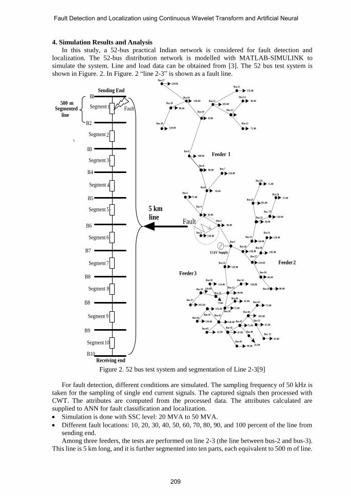
4. Simulation Results and Analysis
In this study, a 52-bus practical Indian network is considered for fault detection and
localization. The 52-bus distribution network is modelled with MATLAB-SIMULINK to
simulate the system. Line and load data can be obtained from [3]. The 52 bus test system is
shown in Figure. 2. In Figure. 2 “line 2-3” is shown as a fault line.
Feeder 1
Fault
Feeder 2
Bus 26
75.00
Feeder 3
Bus 37
Bus 36
90.00
Bus 46
Bus 45Bus 42
45.00
45.00
0045.
Bus 51
75.00
45.00
Bus 47
105.00
75.00
Bus 50
Bus 49
120.00
Bus 390075.
45.00
Bus 41
135.00
Bus 43
105.0000 75.
Bus 40
90.00
120.00Bus 33
114.00
Bus 35
Bus 38
120.00 Bus 29 90.00
60.00
Bus 28
Bus 34
Bus 32
120.00
Bus 27
150.00
105.00
120.00
Bus 30
150.00
Bus 31
60.00
Bus 20
Bus 21
Bus 22 120.00
30.00
105.00
75.00
Bus 24
Bus 25
90.00
120.00
Bus 3
Bus 2
30.00
Bus 4
30.00
Bus 6
75.00
Bus 5
120.00
Bus 7Bus 8
90.00
180.00
Bus 9
75.00
90.00
135.00
Bus 15
Bus 14
Bus 12
105.00
45.00
Bus 11
Bus 10
120.00
Bus 16
120.00
90.00
120.00
Bus 18
Bus 19
Bus 17
Bus 13
Bus 23
Bus 1
Bus 44
150.00
Bus 48Bus 52
45.00
11 kV Supply
5 km
line
Segmented line
500 m
Sending End
Receiving end
Segment 1
Segment 3
Segment 2
Segment 4
Segment 5
Segment 6
Segment 7
Segment 8
Segment 9
Segment 10
Fault
B2
B3
B4
B5
B6
B8
B7
B8
B9
B10
B1
Figure 2. 52 bus test system and segmentation of Line 2-3[9]
For fault detection, different conditions are simulated. The sampling frequency of 50 kHz is
taken for the sampling of single end current signals. The captured signals then processed with
CWT. The attributes are computed from the processed data. The attributes calculated are
supplied to ANN for fault classification and localization.
• Simulation is done with SSC level: 20 MVA to 50 MVA.
• Different fault locations: 10, 20, 30, 40, 50, 60, 70, 80, 90, and 100 percent of the line from
sending end.
Among three feeders, the tests are performed on line 2-3 (the line between bus-2 and bus-3).
This line is 5 km long, and it is further segmented into ten parts, each equivalent to 500 m of line.
Fault Detection and Localization using Continuous Wavelet Transform and Artificial Neural
209

The Line segment model is shown in Figure. 2. These line segments represent different locations
of a particular line. On this line, different types of faults are simulated in 10 different locations
with 20, 25, 30, 35, 40, 45 and 50 MVA source short-circuit level to build the training set. All
the measurements are taken from sending end (node B1 in Figure. 2 segmentation model) of the
line. Some of the three-phase current signals obtained from bus-2 is shown in Figure. 3 (a)-(d)
which correspond L-G (line to ground) fault, L-L-G (double line to ground) fault, 3ph-G (3-
phase to ground) fault, and L-L (line to line) fault, respectively. These transient signals need to
be processed in time-frequency domain for extracting the information. In this study, the CWT is
selected as a signal-processing tool.
Figure 3. 3-phase current waveform captured from 52-bus radial distribution system for the
different type of fault; (a) 3-phase current waveform for L-G fault, (b) 3-phase current
waveform for L-L-G fault, (c) 3-phase current waveform for 3ph-G fault, (d) 3-phase current
waveform for L-L fault.
Various signal-processing tools such as FFT, short time Fourier transform (STFT) and
wavelet, etc. are available which can perform frequency or time-frequency domain analysis.
However, the transient signals for faults are non-stationary. The FFT is only suitable for
stationary signals, as it does not carry the time information. On the other hand, the STFT provider
a time-frequency transformation but it has a resolution problem due to its fixed window length.
The CWT eliminates all the shortcomings of STFT and becomes a much favourite signal-
processing tool to be used for fault transient analysis.
A. Mother-Wavelet and Scale Selection
The frequency domain response of the fault current signals indicates the presence of third
harmonics. Therefore, to implement CWT, proper mother wavelet and scale selection is the most
important thing to be taken care of. After applying ‘scalogram’ technique on various mother
wavelets such as ‘coiflet3’, ‘Daubechies4’, and ‘morlet’ etc. the proper scales are selected to
analyze the third harmonics in the current signal. The selected scale for “coiflet3” mother wavelet
is 234, 235, 236, 247 and for “Daubechies4”, the appropriate scales are 237, 238, 239, 240.
Whereas, the scales selected for ‘morlet’ wavelet transform are 270, 271, 272, and 274. Therefore,
from 3-phase fault current signals captured from different nodes, the CWT coefficients are
obtained. Different source short-circuits level and fault location are considered for four different
predominant fault types.
0 0.02 0.04 0.06 0.08 0.1-500
0
500
Time (ms)
Cu
rren
t (A
)
0 0.02 0.04 0.06 0.08 0.1-500
0
500
Time (ms)
Cu
rren
t (A
)
0 0.02 0.04 0.06 0.08 0.1-500
0
500
Time (ms)
Cu
rren
t (A
)
0 0.02 0.04 0.06 0.08 0.1-500
0
500
Time (ms)
Cu
rren
t (A
)
Phase a Phase b Phase c
(d)
(b)(a)
(c)
Himadri Lala, et al.
210

Figure 4. 3D CWT plot for different fault current signals with ‘coiflet3’ as mother wavelet and
in 22 to 25 scale; (a) CWT plot for L-G fault, (b) CWT plot for L-L-G fault, (c) CWT plot for
3ph-G fault, (d) CWT plot for L-L fault.
Figure 4 (a)-(d) represents the 3D CWT coefficient plots for various faults. Here, in these
plots, three axes are time (x-axis), scale (y-axis) and coefficients (z-axis). Thus, time localization
of the harmonic frequencies with different amplitude occurs.
B. Feature Selection for Detection and Localization Algorithm
The problem of feature selection is to take a set of candidate features and select a subset that
performs the best under some classification system. This procedure can reduce not only the cost
of recognition by reducing the number of features that need to be collected, but in some cases, it
can also provide better accuracy due to finite sample size effect and lesser training time too.
Feature selection needs two parameters.
I. Attribute evaluator
II. Method
In this case, correlation-based feature selection (CFS) subset evaluator is used for evaluating
all the attributes regarding the correlation coefficients and the best-first search algorithm is used
for searching the best features among all. Total 120 features (RMS, standard deviation, crest
factor, mean, maxima, minima, kurtosis, variance, skewness and median for 3 phases and in four
different scales) are initially considered for the detection and localization purpose, which later
reduced to 12 (RMS of 3 phases and four different scales) attributes. With the minimization of
the total number of attributes by 1/10, the entire training time has also gone down accordingly.
This attribute selection was performed in WEKA.
C. Fault Detection and Faulty Line Detection Results
When a fault occurs, it is the very much primary thing to identify or detect the fault type to
understand the severity of the fault. During the fault, the breaker trips at the feeder end. The
current signals captured from the feeder also taken for the further analysis to determine fault type.
Initially, CWT coefficients are calculated, and further, the statistical features/attributes (RMS)
are derived from the CWT coefficients. Thus, total 12 features/attributes are obtained (i.e., for
3-phases - four different scales). Four-class fault type classification using 10-fold cross-
validation analysis result is presented in Table 1. The confusion matrix for classification is shown
in Table 2. Figure 5 shows the graphical representation of fault classification clustering plot with
ANN. It represents the graphical training result using ANN for fault classification.
200400 600
8001000
237
238
239
2400
1000
2000
Time (or Space) bScales a
CO
EF
S
200400
600800
1000
237
238
239
2400
1000
2000
Time (or Space) bScales a
CO
EF
S
200400
600800
1000
237
238
239
2400
1000
2000
Time (or Space) bScales a
CO
EF
S
200400
600800
1000
237
238
239
2400
1000
2000
Time (or Space) bScales a
CO
EF
S
(a) (b)
(d)(c)
Fault Detection and Localization using Continuous Wavelet Transform and Artificial Neural
211

Table 1. Four class fault type classification results using 10-fold cross-validation
Table 2. Confusion matrix for classification of faults using cross-validation
Table 3. Faulty line detection results using 10-fold cross-validation
for the different type of faults
Figure 5. Clustering plot for fault classification using ANN
In fault detection and localization, the sampling frequency is considered 50 kHz. However,
from the fault detection results, it is evident that the CWT-ANN based algorithm successfully
detects the fault type among four different classes. In fault classification, the data used for signal
processing and further analysis is captured from the faulty feeder. In the next stage, faulty line
detection is very much essential to localize the fault successfully. The signals are recorded from
sending-end of all the lines. Captured signals then pass through CWT and the features It shows
0.01 0.02 0.03 0.040.01
0.015
0.02
0.025
0.03
0.035
0.04
Target(T)
Ou
tpu
t(Y
)~=
1*T
arge
t +
0.0
0015
Data
Fit
Y = T
3Ph-G
L-L-G
L-L
L-G
(Sampling frequency: 50kHz, fault location: 0, 20, 30, 40, 50, 60, 70, 80, 90, 100% of the line)
No of data
for each class
Total data in
training set Classification accuracy
7000 28000 100%
A B C D Classified as
7000 0 0 0 A=L-G
0 7000 0 0 B=L-L-G
0 0 7000 0 C=L-L
0 0 0 7000 D=3ph-G
( Sampling frequency: 50kHz, fault location: 10% of the line)
Fault Type
No of
healthy
samples
No of
faulty
samples
No of attributes Classification
accuracy
L-G 1700 100 12 (RMS of CWT
coefficients of
3Phase current
signals in four
scales)
100%
L-L-G 1700 100 100%
3Ph-G 1700 100 100%
L-L 1700 100 100%
Himadri Lala, et al.
212

the detailed method, result and the efficiency of the CWT-ANN based algorithm. Thus the
overall comparison between [3] and the current study is established. Finally, these features help
to detect the faulty line as ANN successfully classifies the faulty line from the healthy line. The
line detection result is shown in Table 3.
D. Fault Localization Results
The fault localization requires precision in the results, as several impedances based methods
are not that accurate in a real scenario. The CWT-ANN based localization algorithm uses the
RMS data calculated for different fault scenario for the training of appropriate neural architecture.
The different fault scenario consists of different fault, different SSC level, and various location.
Table 4 corresponds to the results for fault location with different mother-wavelet and different
type of fault. At the end of the analysis using several mother wavelets and ANN it is found that
the error (the difference between actual fault distance and the average network output) lies nearly
in a range of 1.15 m to 1.63 m with Daubechies4 mother-wavelet, which is reasonably good,
compared to the previous studies. The other mother-wavelets ‘Coiflet3’ and ‘Morlet’ are also
performing well after selecting proper scale. But, the results show the superiority of ‘Daubechies'
mother-wavelet over others on the basis of performance error.
Table 4. Fault localization results using CWT-ANN based algorithm
Pre
sen
t W
ork
Fault
Type
Mother
Wavelet
FFNN
Architecture
Number
of
Epochs
Performance
Error
Error in
Distance(m)
L-G
Morlet
8:8:1
1000 1.83e-07 1.59
L-L-G 1000 3.44e-07 2.16
L-L 1000 1.13e-07 1.22
3Ph-G 1000 3.13e-07 2.11
L-G
Coiflet3
301 9.98e-08 1.14
L-L-G 1000 1.08e-07 1.22
L-L 174 9.87e-08 1.20
3Ph-G 1000 1.78e-07 1.61
L-G
Daubechies4
136 9.49e-08 1.15
L-L-G 141 9.91e-08 1.22
L-L 139 9.41e-08 1.23
3Ph-G 1000 1.76e-07 1.63
Figure 6. Training performance plot of fault localization using ANN for L-G fault with
different mother wavelets; (a) Morlet, (b) Coiflet3, (c) Daubechies4.
0 500 1000
10-5
100
Mea
n S
qu
ared
Err
or (
mse
)
Epochs
Train
Best
Goal
0 100 200 300
10-5
100
Mea
n S
qu
ared
Err
or (
mse
)
Epochs
Train
Best
Goal
0 50 100 150
10-5
100
Mea
n S
qu
ared
Err
or (
mse
)
Epochs
Train
Best
Goal
Best Training Performance
is 1.8317e-07 at epoch 1000
Best Training Performance
is 9.4953e-08 at epoch 136
Best Training Performance
is 9.9855e-08 at epoch 301
(a) (b) (c)
Fault Detection and Localization using Continuous Wavelet Transform and Artificial Neural
213
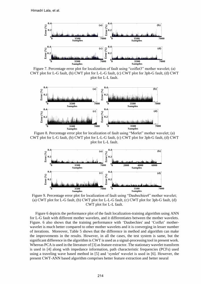
Figure 7. Percentage error plot for localization of fault using “coiflet3” mother wavelet; (a)
CWT plot for L-G fault, (b) CWT plot for L-L-G fault, (c) CWT plot for 3ph-G fault, (d) CWT
plot for L-L fault.
Figure 8. Percentage error plot for localization of fault using “Morlet” mother wavelet; (a)
CWT plot for L-G fault, (b) CWT plot for L-L-G fault, (c) CWT plot for 3ph-G fault, (d) CWT
plot for L-L fault.
Figure 9. Percentage error plot for localization of fault using “Daubechies4” mother wavelet;
(a) CWT plot for L-G fault, (b) CWT plot for L-L-G fault, (c) CWT plot for 3ph-G fault, (d)
CWT plot for L-L fault.
Figure 6 depicts the performance plot of the fault localization-training algorithm using ANN
for L-G fault with different mother wavelets, and it differentiates between the mother wavelets.
Figure. 6 also shows that the training performance with ‘Daubechies' and ‘Coiflet’ mother-
wavelet is much better compared to other mother wavelets and it is converging in lesser number
of iterations. Moreover, Table 5 shows that the difference in method and algorithm can make
the improvements in the results. However, in all the cases, the test system is same, but the
significant difference in the algorithm is CWT is used as a signal-processing tool in present work.
Whereas PCA is used in the literature of [3] as feature extractor. The stationary wavelet transform
is used in [4] along with impedance information, path characteristic frequencies (PCFs) used
using a traveling wave based method in [5] and ‘symlet' wavelet is used in [6]. However, the
present CWT-ANN based algorithm comprises better feature extraction and better neural
0 3500 70000
0.2
0.4
Err
or (
%)
Samples0 3500 7000
0
0.2
0.4
Err
or (
%)
Samples
0 3500 70000
0.2
0.4E
rror
(%
)
Samples0 3500 7000
0
0.2
0.4
Err
or (
%)
Samples
(a) (b)
(d)(c)
0 3500 70000
0.2
0.4
Samples
Err
or (
%)
0 2000 4000 60000
0.2
0.4
Samples
Err
or (
%)
0 3500 70000
0.2
0.4
Samples
Err
or (
%)
0 3500 70000
0.2
0.4
Samples
Err
or (
%)
(a) (b)
(d)(c)
0 3500 70000
0.2
0.4
Samples
Err
or
(%)
0 3500 70000
0.2
0.4
Samples
Err
or
(%)
0 3500 70000
0.2
0.4
Samples
Err
or
(%)
0 3500 70000
0.2
0.4
Samples
Err
or
(%)
(a) (b)
(c) (d)
Himadri Lala, et al.
214
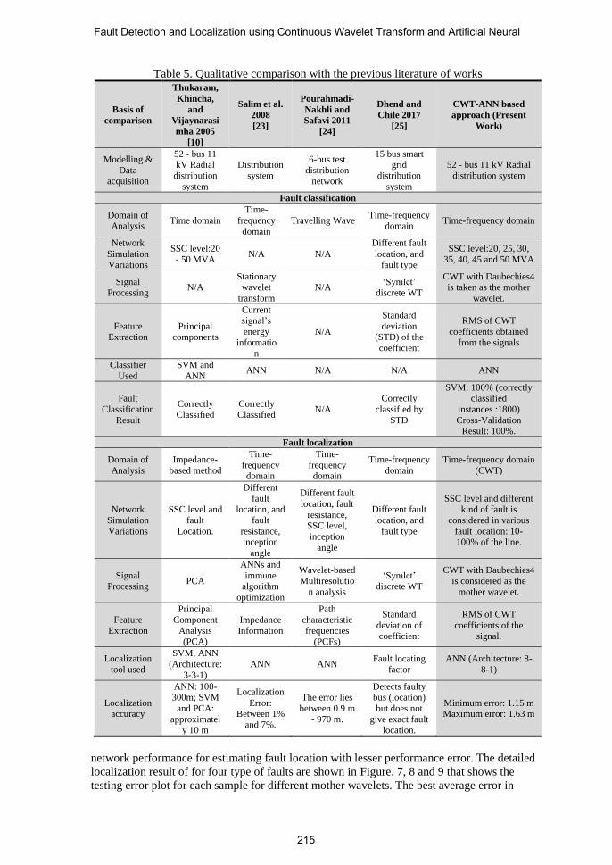
Table 5. Qualitative comparison with the previous literature of works
Basis of
comparison
Thukaram,
Khincha,
and
Vijaynarasi
mha 2005
[10]
Salim et al.
2008
[23]
Pourahmadi-
Nakhli and
Safavi 2011
[24]
Dhend and
Chile 2017
[25]
CWT-ANN based
approach (Present
Work)
Modelling &
Data acquisition
52 - bus 11 kV Radial
distribution
system
Distribution
system
6-bus test
distribution network
15 bus smart grid
distribution
system
52 - bus 11 kV Radial
distribution system
Fault classification
Domain of Analysis
Time domain
Time-
frequency
domain
Travelling Wave Time-frequency
domain Time-frequency domain
Network
Simulation
Variations
SSC level:20
- 50 MVA N/A N/A
Different fault
location, and
fault type
SSC level:20, 25, 30,
35, 40, 45 and 50 MVA
Signal
Processing N/A
Stationary wavelet
transform
N/A ‘Symlet’
discrete WT
CWT with Daubechies4 is taken as the mother
wavelet.
Feature Extraction
Principal components
Current signal’s
energy
information
N/A
Standard
deviation (STD) of the
coefficient
RMS of CWT
coefficients obtained
from the signals
Classifier
Used
SVM and
ANN ANN N/A N/A ANN
Fault
Classification
Result
Correctly Classified
Correctly Classified
N/A
Correctly
classified by
STD
SVM: 100% (correctly classified
instances :1800)
Cross-Validation Result: 100%.
Fault localization
Domain of
Analysis
Impedance-
based method
Time-
frequency domain
Time-
frequency domain
Time-frequency
domain
Time-frequency domain
(CWT)
Network
Simulation
Variations
SSC level and
fault
Location.
Different
fault location, and
fault
resistance, inception
angle
Different fault
location, fault
resistance, SSC level,
inception
angle
Different fault
location, and
fault type
SSC level and different kind of fault is
considered in various
fault location: 10- 100% of the line.
Signal Processing
PCA
ANNs and
immune algorithm
optimization
Wavelet-based
Multiresolutio
n analysis
‘Symlet’ discrete WT
CWT with Daubechies4
is considered as the
mother wavelet.
Feature
Extraction
Principal Component
Analysis
(PCA)
Impedance
Information
Path characteristic
frequencies
(PCFs)
Standard
deviation of coefficient
RMS of CWT
coefficients of the signal.
Localization tool used
SVM, ANN
(Architecture:
3-3-1)
ANN ANN Fault locating
factor ANN (Architecture: 8-
8-1)
Localization accuracy
ANN: 100-300m; SVM
and PCA:
approximately 10 m
Localization
Error: Between 1%
and 7%.
The error lies
between 0.9 m
- 970 m.
Detects faulty bus (location)
but does not
give exact fault location.
Minimum error: 1.15 m Maximum error: 1.63 m
network performance for estimating fault location with lesser performance error. The detailed
localization result of for four type of faults are shown in Figure. 7, 8 and 9 that shows the
testing error plot for each sample for different mother wavelets. The best average error in
Fault Detection and Localization using Continuous Wavelet Transform and Artificial Neural
215

localization is only 1.15 m to 1.63 m with Daubechies4 mother-wavelet, which proves the
efficiency of the proposed algorithm compared to existing impedance based algorithms. Table
5 represents a comparison of the methods as well as results with [3]–[6] as different methods
have been applied to the distribution systems to detect and localize faults. Given the
comparison, the present study offers better accuracy than others do. The methods used in [4]–
[6] localizes the faulty bus. Moreover, unlike present study, they do not pinpoint the exact fault
location accurately.
E. Fault Detection and Localization under Dynamically Changing Load
The power system is dynamically changing regarding topology, loading, etc. The impact of
this change mainly comes due to the dynamically changing load [15]. With the change in load,
the steady-state value of the current also varies. Thus, the pattern of the transient also changes
for different loading conditions. In this scenario, it is essential to detect and localize fault
accurately. In this work, along with SSC level, the load has also been varied, and the performance
of fault classification and localization algorithm is recorded. Two types of loading condition
considered here are uniformly varying load (20%, 50%, 70%, and 100% of above base load value)
in all buses and randomly varying load in all busses. These conditions are taken into account
while capturing the signals for ten different locations and 7 SSC level for building training and
testing data for ANN.
Figure 10. Percentage error plot for fault localization under different load variation; (a) 20%
increase in load (uniform), (b) 50% increase in load (uniform), (c) 70% increase in load
(uniform), (d) 100% increase in load (uniform), (e) Non-uniform load variation.
- Uniformly changing load
The performance of CWT-ANN based fault detection and localization algorithm is shown below.
Table 6 shows the classification accuracy for the cross-validation analysis. Figure.10 (a, b, c, d)
represents the fault localization accuracy under varying loads condition on the 52-bus system.
For classification, there are 400 samples for each type of fault and the Total data in training set
is1600, which gives a classification accuracy of 100%. In case of localization Figure.10 (a, b, c,
d) shows the four testing results for different loading conditions with the result of 100 test
samples each. The average testing error in 20%, 50%, 70% and 100% increase in load are 4m,
2m, 0.5m and 3m respectively. This is much more accurate than the results reported in the
existing works of literature under load variation.
- Randomly changing load
In practical cases, the system load changes non-uniformly and it is necessary to consider non-
uniform load variation in the system while testing the CWT-ANN based algorithm. In this work,
0 20 40 60 80 1000
0.5
1
Samples
Erro
r (
%)
0 20 40 60 80 1000
0.5
1
Samples
Erro
r (
%)
0 20 40 60 80 1000
0.5
1
Samples
Erro
r (
%)
0 20 40 60 80 1000
0.5
1
Samples
Erro
r (
%)
0 10 20 30 40 50 60 70 80 90 1000
0.5
1
1.5
Samples
Erro
r (
%)
(a) (b)
(d)(c)
(e)
Himadri Lala, et al.
216

system load is varied non-uniformly for each bus to build the training data for the neural network.
Seven different load data set in which load at each bus is randomly varied is used in this case
study. The testing result considering non-uniform load variation is shown in Figure. 10 (e). A
total number of training data for the training of ANN is 7000.
Table 6. Comparison of fault localization results under load variation
Loading Fault
Type
FFNN
Architecture
Number
of
Training
Samples
Number
of
Epochs
Best
Performance
Error in
Distance(m)
Computational
Time(sec)
Normal
L-G
5:8:1
1750 120 9.99e-06 5.56 2.42
20%
increase 900 60 9.46e-07 4 0.94
50%
increase 900 80 9.53e-07 2 1.20
70%
increase 900 113 7.74e-07 0.5 1.60
100%
increase 900 226 9.94e-07 3 3.06
No-
Uniform 7000 500 3.047e-05 4.45 26.91
In Table 6, the performance of CWT-ANN based algorithm under different load variation is
shown, which shows the ability of the algorithm in working under randomly load variation. In
case of randomly changing load, the number of training samples required is much higher than
other cases. It also needs more iteration for achieving the performance goal, thus, resulting more
computational time. The computational time would not be an issue as several high-performance
processors are available which are capable of reducing the computational time.
5. Conclusion
In the problem of fault classification, time-frequency domain response is efficiently working
to discriminate the faults in much lesser computational time. Here, among all features, the most
crucial feature is found to be RMS, which offers a better accuracy for both detection and
localization. This algorithm provides a very efficient scheme to detect and localize faults in radial
distribution systems. With a good percentage of accuracy in detection, this algorithm has also
minimized the localization error between 1.15 m and 1.63 m with “Daubechies4” mother-
wavelet, which is a much better result as compared to the results reported in the similar works
with other mother wavelets. The proposed CWT-ANN algorithm also gives promising in load
varying conditions. This algorithm provides 100% classification accuracy for both fault type
detection and the faulty line detection. The testing results describe the superiority of the
algorithm as it successfully detects and localizes the faults with a minimum error margin.
However, there is an ample amount of future scope in this field of research, which will emphasize
the reduction of errors considering more parameters and computational burden in the localization
fault in distribution systems.
6. References
[1]. S. M. Amin and B. F. F. Wollenberg, “Toward a smart grid: power delivery for the 21st
century,” IEEE Power and Energy Magazine, vol. 3, no. 5, pp. 34–41, 2005.
[2]. A. Borghetti, M. Bosetti, M. Di Silvestro, C. A. Nucci, and M. Paolone, “Continuous-
wavelet transform for fault location in distribution power networks: Definition of mother
wavelets inferred from fault originated transients,” IEEE Trans. Power Syst., vol. 23, no. 2,
pp. 380–388, 2008.
[3]. D. Thukaram, H. P. Khincha, and H. P. Vijaynarasimha, “Artificial neural network and
support vector machine approach for locating faults in radial distribution systems,” IEEE
Trans. Power Deliv., vol. 20, no. 2 I, pp. 710–721, 2005.
Fault Detection and Localization using Continuous Wavelet Transform and Artificial Neural
217

[4]. R. H. Salim, K. R. C. de Oliveira, A. D. Filomena, M. Resener, and A. S. Bretas, “Hybrid
fault diagnosis scheme implementation for power distribution systems automation,” IEEE
Trans. Power Deliv., vol. 23, no. 4, pp. 1846–1856, 2008.
[5]. M. Pourahmadi-Nakhli and A. A. Safavi, “Path characteristic frequency-based fault
locating in radial distribution systems using wavelets and neural networks,” IEEE Trans.
Power Deliv., vol. 26, no. 2, pp. 772–781, 2011.
[6]. M. H. Dhend and R. H. Chile, “Fault diagnosis of smart grid distribution system by using
smart sensors and symlet wavelet function,” J. Electron. Test., vol. 33, no. 3, pp. 329–338,
2017.
[7]. C. Fukui and J. Kawakami, “An expert system for fault section estimation using
information from protective relays and circuit breakers,” IEEE Power Eng. Rev., vol. PER-
6, no. 10, pp. 29–30, 1986.
[8]. C. K. Jung, K. H. Kim, J. B. Lee, and B. Klöckl, “Wavelet and neuro-fuzzy based fault
location for combined transmission systems,” Int. J. Electr. Power Energy Syst., vol. 29,
no. 6, pp. 445–454, 2007.
[9]. C. S. Chang, L. Tian, and F. S. Wen, “A new approach to fault section estimation in power
systems using ant system,” Electr. Power Syst. Res., vol. 49, no. 1, pp. 63–70, 1999.
[10]. P. K. Dash and S. R. Samantaray, “A novel distance protection scheme using time-
frequency analysis and pattern recognition approach,” Int. J. Electr. Power Energy Syst.,
vol. 29, no. 2, pp. 129–137, 2007.
[11]. P. S. Bhowmik, P. Purkait, and K. Bhattacharya, “A novel wavelet assisted neural network
for transmission line fault analysis,” Proc. INDICON 2008 IEEE Conf. Exhib. Control.
Commun. Autom., vol. 1, no. 5, pp. 223–228, 2008.
[12]. R. Polikar, “The Wavelet Tutorial,” Comp. A J. Comp. Educ., vol. 17, pp. 1–14, 2009.
[13]. P. Purkait and S. Chakravorti, “Wavelet transform-based impulse fault pattern recognition
in distribution transformers,” IEEE Trans. Power Deliv., vol. 18, no. 4, pp. 1588–1589,
2003.
[14]. M. Mirzaei, M. Z. a A. Kadir, E. Moazami, and H. Hizam, “Review of fault location
methods for distribution power system,” Aust. J. Basic Appl. Sci., vol. 3, no. 3, pp. 2670–
2676, 2009.
[15]. J. Mora, J. Meléndez, M. Vinyoles, J. Sánchez, and M. Castro, “An overview to fault
location methods in distribution system based on single end measures of voltage and
current,” in International Conference on Renewable Energies and Power Quality
(ICREPQ’04), 2004, vol. 1, no. 2, pp. 235–239.
[16]. M. M. Saha, R. Das, P. Verho, and D. Novosel, “Review of fault location techniques for
distribution systems,” in Power Systems and Communications Infrastructures for the future,
2002, no. September, pp. 1–6.
[17]. A. Yadav and A. Swetapadma, “A single ended directional fault section identifier and fault
locator for double circuit transmission lines using combined wavelet and ANN approach,”
Int. J. Electr. Power Energy Syst., vol. 69, pp. 27–33, 2015.
[18]. S. A. Saleh, C. R. Moloney, and M. Azizur Rahman, “Implementation of a dynamic voltage
restorer system based on discrete wavelet transforms,” Power Deliv. IEEE Trans., vol. 23,
no. 4, pp. 2366–2375, 2008.
[19]. S. R. Samantaray, P. K. Dash, and G. Panda, “Fault classification and location using HS-
transform and radial basis function neural network,” Electric Power Systems Research, vol.
76. pp. 897–905, 2006.
[20]. H. F. Zhang, Z. C. Pan, and Z. G. Tian, “Detection and location of ground faults using a
discernible signal,” in Proceedings of the IEEE Power Engineering Society Transmission
and Distribution Conference, 2005, vol. 2005, pp. 1–4.
[21]. H. Yong, C. Minyou, and Z. Jinqian, “High impedance fault identification method of the
distribution network based on discrete wavelet transformation,” in 2011 International
Conference on Electrical and Control Engineering, 2011, pp. 2262–2265.
Himadri Lala, et al.
218

[22]. K. Figureueiredo, J. a. Moor Neto, L. Lovisolo, J. C. dos Santos Rocha, and L. de Menezes
Laporte, “Location of faults generating short-duration voltage variations in distribution
systems regions from records captured at one point and decomposed into damped sinusoids,”
IET Gener. Transm. Distrib., vol. 6, no. 12, pp. 1225–1234, 2012.
[23]. H. Lala and S. Karmakar, “Continuous wavelet transform and artificial neural network
based fault diagnosis in 52 bus hybrid distributed generation system,” in IEEE Students
Conference on Engineering and Systems (SCES), 2015, 2015, pp. 1–6.
[24]. S. G. Mallat, “Multifrequency channel decompositions of images and wavelet models,”
IEEE Trans. Accoustic, Speech Signal Process., vol. 37, no. 12, 1989.
[25]. Stephane G. Mallat, “A theory for multiresolution signal decomposition : The wavelet
representation,” IEEE Trans. Patern Anal. Mach. Intell., vol. 11, no. 7, pp. 674–693, 1989.
[26]. Ingrid Doubenchies, “The wavelet transform , time-frequency localization and signal
analysis,” IEEE Trans. Inf. Theory, vol. 36, no. 5, 1990.
[27]. O. Rioul and M. Vetierli, “Wvelets and signal processing,” IEEE Signal Process. Mag., vol.
8, no. 4, pp. 14–38, 1991.
[28]. D. E. Rumelhart, G. E. Hinton, and R. J. Williams, “Learning representations by back-
propagating errors,” Nature, vol. 323, no. 6088, pp. 533–536, 1986.
[29]. P. J. Werbos, “Beyond regression: New tools for prediction and analysis in the behavioral
sciences,” MIT Press, 1974.
Himadri Lala was born in Suri, India, on 27th October, 1987. He received his
Bachelor’s degree in electrical engineering from West Bengal University of
Technology, India, in 2010. He received the M.E. degrees from Indian Institute
of Engineering, Science, and Technology (IIEST), Shibpur {Formerly, Bengal
Engineering and Science University} in 2012. Currently he is a Ph.D. Research
Scholar at the Department of Electrical Engineering, NIT Rourkela, India. His
research interests include Detection and localization of power system
transients using various signal processing and soft computing techniques.
Subrata Karmakar was born in Balarampur, India, in 1981. He received the
Bachelor’s degree (with honors) in electrical engineering from the University
of Burdwan, Bardhaman, India, in 2004, and the M.Tech. and Ph.D. degrees
from the National Institute of Technology (NIT), Durgapur, India, in 2006 and
2011, respectively. He is currently an Assistant Professor with the Department
of Electrical Engineering, NIT, Rourkela, India. His research interests include
online monitoring of high-voltage power system equipment, detection of fault
using signal processing and soft computing technique.
Sanjib Ganguly was born on in India in 1981. He obtained Bachelor of
Engineering degree in Electrical Engineering from Indian Institute of
Engineering, Science, and Technology (IIEST), Shibpur {Formerly, Bengal
Engineering and Science University} in 2003. He received Master of Electrical
Engineering degree from Jadavpur University, Kolkata in 2006. He was
awarded with the Ph.D degree from the Department of Electrical Engineering,
Indian Institute of Technology Kharagpur in 2011. He worked in the Tata
Power Company Ltd., as a Sr. officer, electrical maintenance of 2×500 MW
thermal power units in Trombay Thermal Power Station, Mumbai from 2006-2007. He worked
as the Assistant Professor in NIT Rourkela from 2011-2015. He is presently working as Assistant
Professor in Indian Institute of Technology Guwahati from 2015. His research interest includes
distribution system planning and optimization, multi-objective optimization, and evolutionary
algorithms.
Fault Detection and Localization using Continuous Wavelet Transform and Artificial Neural
219