fatigue testing and data analysis of welded steel
TRANSCRIPT
University of New Orleans University of New Orleans
ScholarWorks@UNO ScholarWorks@UNO
University of New Orleans Theses and Dissertations Dissertations and Theses
Spring 5-17-2013
Fatigue Testing and Data Analysis of Welded Steel Cruciform Fatigue Testing and Data Analysis of Welded Steel Cruciform
Joints Joints
Alina Shrestha [email protected]
Follow this and additional works at: https://scholarworks.uno.edu/td
Part of the Mechanics of Materials Commons, Structural Engineering Commons, Structural Materials
Commons, and the Structures and Materials Commons
Recommended Citation Recommended Citation Shrestha, Alina, "Fatigue Testing and Data Analysis of Welded Steel Cruciform Joints" (2013). University of New Orleans Theses and Dissertations. 1670. https://scholarworks.uno.edu/td/1670
This Thesis is protected by copyright and/or related rights. It has been brought to you by ScholarWorks@UNO with permission from the rights-holder(s). You are free to use this Thesis in any way that is permitted by the copyright and related rights legislation that applies to your use. For other uses you need to obtain permission from the rights-holder(s) directly, unless additional rights are indicated by a Creative Commons license in the record and/or on the work itself. This Thesis has been accepted for inclusion in University of New Orleans Theses and Dissertations by an authorized administrator of ScholarWorks@UNO. For more information, please contact [email protected].
i
Fatigue Testing and Data Analysis of Welded Steel Cruciform Joints
A Thesis
Submitted to the Graduate Faculty of the
University of New Orleans
in partial fulfillment of the
requirements for the degree of
Master of Science
In
Engineering
Naval Architecture & Marine Engineering
by
Alina Shrestha
B.S., University of New Orleans, 2011
May, 2013
ii
Acknowledgements
I would like to acknowledge and express my sincere gratitude to several individuals who helped make this
thesis possible by supporting and guiding as well as contributing time out of their busy schedules for the
preparation and completion of this study.
First and foremost, my gratitude goes to Dr. Pingsha Dong, for making this research possible. His patience and
steadfast encouragement, along with unfailing support as my thesis advisor, are greatly appreciated. Indeed, I
would not be able to put together this topic, in absence of his guidance.
Besides my advisor, I will always appreciate the professors in the School of Naval Architecture and Marine
Engineering for their untiring effort in encouraging me, and all the students as a whole to pursue academic
and professional growth. Also, I would like to thank George Morrissey and Ryan Thiel for being available to
help whenever needed.
I would like to acknowledge Mr. Larry DeCan for all of the invaluable help and timely advice that he provided
throughout the project to keep it running more smoothly.
My sincere thanks also goes to my fellow coworkers for the stimulating discussions, constructive criticisms,
for long working hours before deadlines, and for all the fun we had in the last two years.
Lastly, I would like to thank my family and my friends for believing in me and supporting me in all my
endeavors.
iii
Table of Contents
List of Figures ................................................................................................................................................ v
List of Tables ............................................................................................................................................... vii
Abstract ...................................................................................................................................................... viii
I. Introduction .......................................................................................................................................... 1
Background ............................................................................................................................................... 1
Objective ................................................................................................................................................... 5
II. Literature Review .................................................................................................................................. 6
Introduction .............................................................................................................................................. 6
Approach ................................................................................................................................................... 6
Review of ABS Fatigue guideline ............................................................................................................... 6
S-N Curve Approach .............................................................................................................................. 7 Joint Classification Scheme ................................................................................................................... 8 Adjustment to the S-N Curves .............................................................................................................. 9 Design Stresses for Fatigue Assessment ............................................................................................. 12
Assessment ............................................................................................................................................. 14
III. Test Procedures & Results .................................................................................................................. 15
Introduction ............................................................................................................................................ 15
Test Method ............................................................................................................................................ 15
Test Material ....................................................................................................................................... 15 Test Specimen ..................................................................................................................................... 15 Test Machine....................................................................................................................................... 17 Test Requirements .............................................................................................................................. 18 Test Procedures .................................................................................................................................. 19
Test Results & Observation ..................................................................................................................... 21
Specimen Pool .................................................................................................................................... 21 Stiffness Measurement Results .......................................................................................................... 21 Thickness Effect Results ...................................................................................................................... 21 Fatigue Failure Path and the Critical Point ......................................................................................... 24
Data Analysis & Discussions .................................................................................................................... 27
Statistical Analysis ............................................................................................................................... 27 Nominal Stress Based Experimental S-N Chart ................................................................................... 27
Comparison of Nominal Stress Based Experimental S-N Curve with ABS Nominal Stress Based Design S-N Curve .................................................................................................................................................... 29
Limitations of Hot-Spot Stress for simple connections....................................................................... 32 IV. Master S-N Curve Representation ......................................................................................................... 34
Equivalent Structural Stress Parameter .................................................................................................. 35
iv
Traction-Based Structural Stress ......................................................................................................... 36 Self-Equilibrating Stress or Notch Stress ............................................................................................ 38
Fatigue Strength Assessment using Master S-N Curve Approach .......................................................... 39
Finite Element Analysis and Structural Stress Calculation .................................................................. 39 Stress Concentration Factor based on Traction Stress ....................................................................... 42 Equivalent Structural Stress Based Experimental S-N Chart ............................................................... 43
Statistical Parameter Comparison of S-N plots based on Equivalent Structural Stress with Nominal Stress Approach ...................................................................................................................................... 45
Conclusion ............................................................................................................................................... 46
V. Conclusions ............................................................................................................................................. 47
References .................................................................................................................................................. 48
Appendices .................................................................................................................................................. 49
Appendix A .............................................................................................................................................. 50
Appendix B .............................................................................................................................................. 55
Stiffness Calculation ............................................................................................................................ 55 Vita .............................................................................................................................................................. 56
v
List of Figures
Figure 1 Different phases of the fatigue life ........................................................................................................................................ 1
Figure 2 Fatigue failure of S.S. Schenectady, Liberty Ship ............................................................................................................ 1
Figure 3: (Left) Hull fracture of passenger ship, S.S. America ; (Right) Floating drill platform, Alexander
Kielland, capsized after fatigue failure in one cross-brace securing the columns ............................................................. 2
Figure 4: Constant amplitude stress history ....................................................................................................................................... 2
Figure 5: Typical S-N curve for constant amplitude tests ............................................................................................................. 3
Figure 6: Approaches to describe the fatigue strength .................................................................................................................. 4
Figure 7: Two-Segment S-N Curve ........................................................................................................................................................... 8
Figure 8: ABS-(A) Offshore S-N Curves for Non-Tubular Details in Air ................................................................................ 10
Figure 9: ABS-(CP) Offshore S-N Curves for Non-Tubular Details in Seawater with Cathodic Protection ........... 11
Figure 10: ABS-(FC) Offshore S-N Curves for Non-Tubular Details in Seawater for Free Corrosion ...................... 12
Figure 11: Stress Gradients (Actual & Idealized) Near a Weld ................................................................................................. 13
Figure 12: Load-Bearing Cruciform Joint (Left); Non-Load-Bearing Cruciform Joint (Right) .................................... 15
Figure 13: Dimensions of a Cruciform Joint, Weld size (S) and Thickness (T) .................................................................. 17
Figure 14: Load-Bearing and Non-Load-Bearing Steel Cruciform Joints received by UNO for Fatigue Testing . 17
Figure 15: MTS Unixial Test Machine at the University of New Orleans .............................................................................. 17
Figure 16: Severe Offset in the Specimen ........................................................................................................................................... 18
Figure 17: Two Major Fatigue Failure Modes Classification ...................................................................................................... 19
Figure 18: Distortion Criteria Check on the Scanned AUTOCAD Pictures of the Specimens: Pass (Left); Fail
(Right) ................................................................................................................................................................................................................ 19
Figure 19: 20 Ton Hydraulic Power Life Bottle Jack ..................................................................................................................... 20
Figure 20: Applied Force over Cycles Plot (Top Left); Displacement over Cycles Plot (Top Right); Specimen
30-A1 (Bottom Left); Stiffness of the Specimen over Cycles Plot (Bottom Right) ........................................................... 22
Figure 21: Fatigue Data of Load-Carrying Cruciform Joints with Applied Stress Range of 30 Ksi............................ 22
Figure 22: Fatigue Data of Load-Carrying Cruciform Joints with Applied Stress Range of 60 Ksi............................ 23
Figure 23: Fatigue Data of Non-Load-Carrying Cruciform Joints with Applied Stress Range of 30 Ksi ................. 23
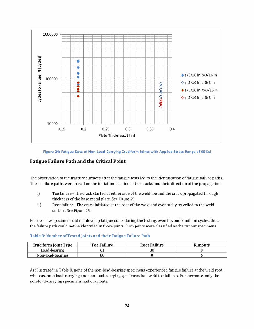
Figure 24: Fatigue Data of Non-Load-Carrying Cruciform Joints with Applied Stress Range of 60 Ksi ................. 24
Figure 25: Fatigue Failure Path: Weld Toe ........................................................................................................................................ 25
Figure 26: Fatigue Failure Path: Weld Root or Weld Throat ..................................................................................................... 25
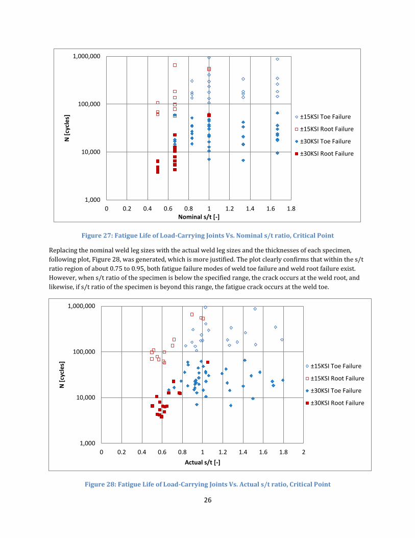
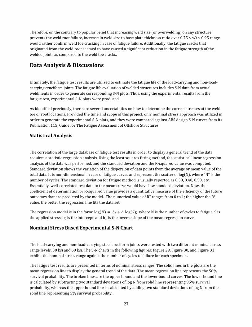
Figure 27: Fatigue Life of Load-Carrying Joints Vs. Nominal s/t ratio, Critical Point ..................................................... 26
Figure 28: Fatigue Life of Load-Carrying Joints Vs. Actual s/t ratio, Critical Point .......................................................... 26
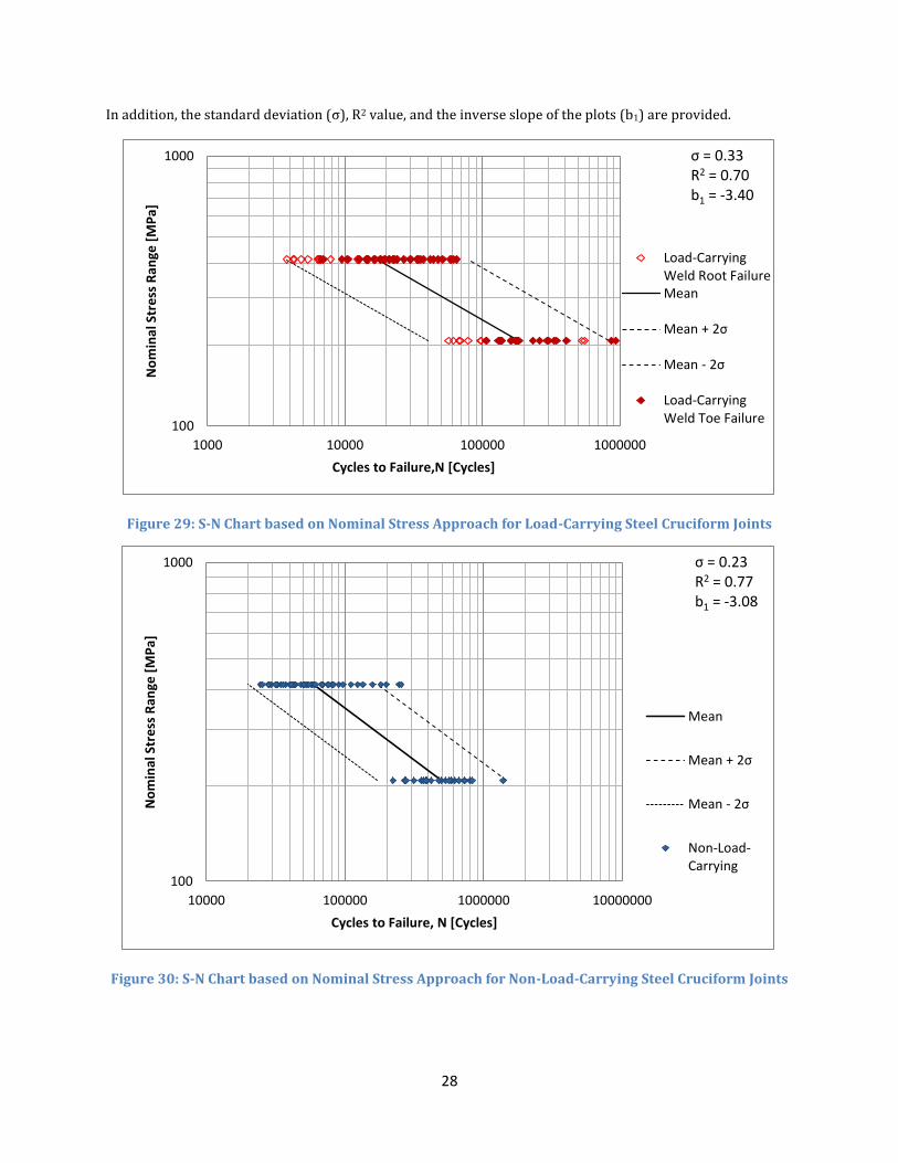
Figure 29: S-N Chart based on Nominal Stress Approach for Load-Carrying Steel Cruciform Joints ...................... 28
Figure 30: S-N Chart based on Nominal Stress Approach for Non-Load-Carrying Steel Cruciform Joints............ 28
Figure 31: S-N Chart based on Nominal Stress Approach for all Steel Cruciform Joints ............................................... 29
Figure 32: Class F Joint Type from ABS Fatigue Design Guidelines ........................................................................................ 30
Figure 33 Class F2 Joint Type from ABS Fatigue Design Guidelines ...................................................................................... 30
Figure 34: ABS Class F2 Design S-N Curve Vs. Experimental S-N Data of Load-Bearing Cruciform Joints with
Weld Toe Failure ........................................................................................................................................................................................... 31
Figure 35: ABS Class W Design S-N Curve Vs. Experimental S-N Data of Load-Bearing Cruciform Joints with
Weld Root Failure ......................................................................................................................................................................................... 31
Figure 36: ABS Class F Design S-N Curve Vs. Experimental S-N Data of Non-Load-Bearing Cruciform Joints .... 32
Figure 37: Illustration of Stress Normal to a Shell Element Model ......................................................................................... 33
Figure 38: Master S-N Curve of Weldments and Statistical Representation of the Mean, Lower Bound, and
Upper Bound Lines from WRC Bulletin ............................................................................................................................................... 34
vi
Figure 39: Through-thickness Structural Stresses Definition: Local Stresses, Structural Stress, and Self-
Equilibrating Stress ...................................................................................................................................................................................... 35
Figure 40: Exposing Three Structural Stress Components in Section A-A in a 2D Cross-Section (Left) and
Section A-A-C-C in a 3D Cross-Section (Right) ................................................................................................................................. 36
Figure 41: Element Group Highlighted to Collect the Nodal Forces for Weld Toe Failure ........................................... 38
Figure 43: A Quarter FE Model of 10 mm Non-Load-Carrying Cruciform Joint ................................................................ 40
Figure 44: Boundary Conditions applied to the FE Model Along the Symmetry Lines .................................................. 40
Figure 45: Von Mises Stress Distribution. Load Applied = 207 MPa. ..................................................................................... 41
Figure 46: Nodal Force Distribution ..................................................................................................................................................... 41
Figure 47: Hypothetical Cut Location at the Weld Toe through Thickness......................................................................... 41
Figure 48: Parametric SCF Curves of Load-Carrying and Non-Load-Carrying Cruciform Joints ............................... 42
Figure 49: Equivalent Structural Stress based S-N Chart for Load-Carrying Specimens .............................................. 44
Figure 50: Equivalent Structural Stress based S-N Chart for Non-Load-Carrying Specimens .................................... 44
Figure 51: Equivalent Structural Stress based S-N Chart for Load-Carrying and Non-Load-Carrying Specimens
............................................................................................................................................................................................................................... 45
vii
List of Tables
Table 1: Details of the Basic "In-Air" S-N Curves .............................................................................................................................. 8
Table 2: Parameters for ABS-(A) Offshore S-N Curves for Non-Tubular Details In Air ................................................. 10
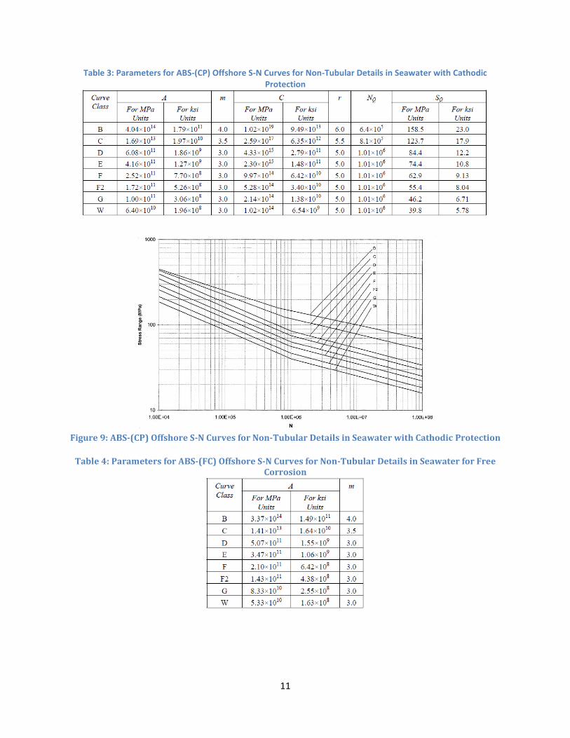
Table 3: Parameters for ABS-(CP) Offshore S-N Curves for Non-Tubular Details in Seawater with Cathodic
Protection ......................................................................................................................................................................................................... 11
Table 4: Parameters for ABS-(FC) Offshore S-N Curves for Non-Tubular Details in Seawater for Free Corrosion
............................................................................................................................................................................................................................... 11
Table 5: Mechanical Properties of the Specimen Material .......................................................................................................... 15
Table 6: Fatigue Weldment Matrix: Load-bearing (left) and non-load-bearing (right)................................................. 16
Table 7: Load Specification for Test of Individual Cruciform Joint ......................................................................................... 18
Table 8: Number of Tested Joints and their Fatigue Failure Path ........................................................................................... 24
Table 9: Traction based Structural Stress Computation from FE Model .............................................................................. 42
Table 10: Comparison of Statistical Parameters of S-N Curves based on Nominal Stress and Equivalent
Structural Stress ............................................................................................................................................................................................ 45
viii
Abstract
In this study, ABS Publication 115, “Guidance on Fatigue Assessment of Offshore Structures” is briefly
reviewed. Emphasis is on the S-N curves based fatigue assessment approach of non-tubular joints, and both
size and environment effects are also considered. Further, fatigue tests are performed to study the fatigue
strength of load-carrying and non-load-carrying steel cruciform joints that represent typical joint types in
marine structures. The experimental results are then compared against ABS fatigue assessment methods,
based on nominal stress approach, which demonstrates a need for better fatigue evaluation parameter. A
good fatigue parameter by definition should be consistent and should correlate the S-N data well. The
equivalent structural stress parameter is introduced to investigate the fatigue behavior of welded joints using
the traction based structural stress approach on finite element models of specimens, and representing the
data as a single Master S-N curve.
Key words: Fatigue, ABS, Size Effect, Master S-N Curve, Equivalent Structural Stress, Traction Stress, Toe
Failure, Root Failure
1
I. Introduction
Background
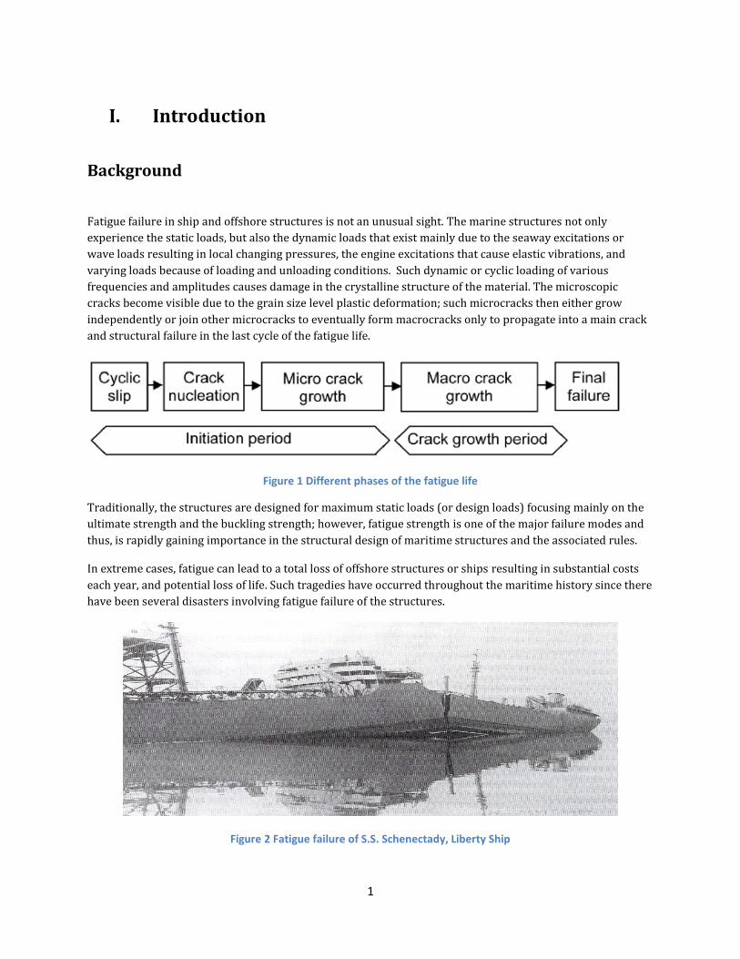
Fatigue failure in ship and offshore structures is not an unusual sight. The marine structures not only
experience the static loads, but also the dynamic loads that exist mainly due to the seaway excitations or
wave loads resulting in local changing pressures, the engine excitations that cause elastic vibrations, and
varying loads because of loading and unloading conditions. Such dynamic or cyclic loading of various
frequencies and amplitudes causes damage in the crystalline structure of the material. The microscopic
cracks become visible due to the grain size level plastic deformation; such microcracks then either grow
independently or join other microcracks to eventually form macrocracks only to propagate into a main crack
and structural failure in the last cycle of the fatigue life.
Figure 1 Different phases of the fatigue life
Traditionally, the structures are designed for maximum static loads (or design loads) focusing mainly on the
ultimate strength and the buckling strength; however, fatigue strength is one of the major failure modes and
thus, is rapidly gaining importance in the structural design of maritime structures and the associated rules.
In extreme cases, fatigue can lead to a total loss of offshore structures or ships resulting in substantial costs
each year, and potential loss of life. Such tragedies have occurred throughout the maritime history since there
have been several disasters involving fatigue failure of the structures.
Figure 2 Fatigue failure of S.S. Schenectady, Liberty Ship

2
Figure 3: (Left) Hull fracture of passenger ship, S.S. America ; (Right) Floating drill platform, Alexander Kielland, capsized after fatigue failure in one cross-brace securing the columns
Historical catastrophes indicate that fatigue strength should be an important consideration while designing
structures. Moreover, these days, every effort is made to increase the power-to-weight ratio of sophisticated
maritime structures, which increases the vibrational problems, reduces the actual structural material, and
thus, results in the reduction of the fatigue strength margin. High-tensile steel is introduced to meet the
demand of reduced structural weight, which normally indicates heightened static strength, but similar fatigue
strength as of mild steel.
High possibility of fatigue failures occur particularly in the welded structures because of the poor fatigue
performance of many welded joints. Welding introduces inhomogeneity in material since additional filler
material is utilized implementing subsequent heating and cooling process. Weld includes all kinds of defects
like inclusions, pores, undercuts etc, and the shape of weld profiles presents geometric variations thus
causing high stress concentrations. Furthermore, welding results in the residual stresses and distortions in
the structure, thus severely affecting the fatigue behavior. Clearly, ships and offshore structures consist of
various weld joints and thus, this emphasizes the need to consider the potential fatigue failure at the design
stage early on in any project.
The fatigue strength of a welded component is defined as the stress range (Δσ) that fluctuates at constant
amplitude, causing failure of the component after a specified number of cycles (N). The stress range is the
difference between the maximum and the minimum stress values, as shown in Figure 4. Similarly, the ratio of
minimum to maximum stress values is denoted by R-ratio. The number of cycles to failure is known as the
fatigue life of the component.
Figure 4: Constant amplitude stress history
3
Several research efforts are ongoing in order to study the effective fatigue strength evaluation approaches for
these welded structures. In addition to that, substantial efforts are made towards the introduction of various
standards and fatigue design codes for the marine industry in order to provide an accurate estimate of fatigue
life of ships and offshore structures. The codes used by several classification societies are based mainly upon
the test data accumulated from fatigue tests on some small-scale specimens integrating the weld detail of
interest, by statistical analysis. They also consider the data from actual fatigue damages in ships and other
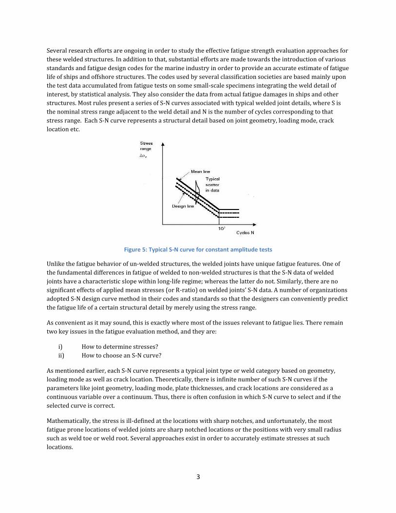
structures. Most rules present a series of S-N curves associated with typical welded joint details, where S is
the nominal stress range adjacent to the weld detail and N is the number of cycles corresponding to that
stress range. Each S-N curve represents a structural detail based on joint geometry, loading mode, crack
location etc.
Figure 5: Typical S-N curve for constant amplitude tests
Unlike the fatigue behavior of un-welded structures, the welded joints have unique fatigue features. One of
the fundamental differences in fatigue of welded to non-welded structures is that the S-N data of welded
joints have a characteristic slope within long-life regime; whereas the latter do not. Similarly, there are no
significant effects of applied mean stresses (or R-ratio) on welded joints’ S-N data. A number of organizations
adopted S-N design curve method in their codes and standards so that the designers can conveniently predict
the fatigue life of a certain structural detail by merely using the stress range.
As convenient as it may sound, this is exactly where most of the issues relevant to fatigue lies. There remain
two key issues in the fatigue evaluation method, and they are:
i) How to determine stresses?
ii) How to choose an S-N curve?
As mentioned earlier, each S-N curve represents a typical joint type or weld category based on geometry,
loading mode as well as crack location. Theoretically, there is infinite number of such S-N curves if the
parameters like joint geometry, loading mode, plate thicknesses, and crack locations are considered as a
continuous variable over a continuum. Thus, there is often confusion in which S-N curve to select and if the
selected curve is correct.
Mathematically, the stress is ill-defined at the locations with sharp notches, and unfortunately, the most
fatigue prone locations of welded joints are sharp notched locations or the positions with very small radius
such as weld toe or weld root. Several approaches exist in order to accurately estimate stresses at such
locations.
4
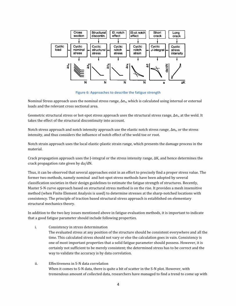
Figure 6: Approaches to describe the fatigue strength
Nominal Stress approach uses the nominal stress range, Δσn, which is calculated using internal or external
loads and the relevant cross sectional area.
Geometric structural stress or hot-spot stress approach uses the structural stress range, Δσs, at the weld. It
takes the effect of the structural discontinuity into account.
Notch stress approach and notch intensity approach use the elastic notch stress range, Δσk, or the stress
intensity, and thus considers the influence of notch effect of the weld toe or root.
Notch strain approach uses the local elastic-plastic strain range, which presents the damage process in the
material.
Crack propagation approach uses the J-integral or the stress intensity range, ΔK, and hence determines the
crack propagation rate given by da/dN.
Thus, it can be observed that several approaches exist in an effort to precisely find a proper stress value. The
former two methods, namely nominal and hot-spot stress methods have been adopted by several
classification societies in their design guidelines to estimate the fatigue strength of structures. Recently,
Master S-N curve approach based on structural stress method is on the rise. It provides a mesh insensitive
method (when Finite Element Analysis is used) to determine stresses at the sharp-notched locations with
consistency. The principle of traction based structural stress approach is established on elementary
structural mechanics theory.
In addition to the two key issues mentioned above in fatigue evaluation methods, it is important to indicate
that a good fatigue parameter should include following properties.
i. Consistency in stress determination
The evaluated stress at any position of the structure should be consistent everywhere and all the
time. This calculated stress should not vary or else the calculation goes in vain. Consistency is
one of most important properties that a solid fatigue parameter should possess. However, it is
certainly not sufficient to be merely consistent; the determined stress has to be correct and the
way to validate the accuracy is by data correlation.
ii. Effectiveness in S-N data correlation
When it comes to S-N data, there is quite a bit of scatter in the S-N plot. However, with
tremendous amount of collected data, researchers have managed to find a trend to come up with
5
S-N curves that marine industry has been using worldwide. Each S-N curve has its upper and
lower limit based on the scatter of the data. The determined stress that falls into the S-N plot
without increasing the scatter band, rather, collapsing the scatter band into fairly narrow band
demonstrates strong data correlation, and hence the accuracy of the fatigue parameter.
Therefore, a good fatigue parameter should not only possess the effectiveness in S-N data
correlation, but also the consistency in stress determination.
Objective
The main objective in this thesis is to review and apply the fatigue design guideline of a major American
marine classification society, American Bureau of Shipping, to several loaded and non-loaded steel cruciform
joints, and experimentally validate the newly developed master S-N approach in comparison with the ABS
guidelines.

6
II. Literature Review
Introduction
Among several classification societies linked to the marine industry, American Bureau of Shipping (ABS) is
one of the major organizations that have been involved in the fatigue technology development. Ship Structure
Committee (SSC) has carried out several fatigue research projects with the funding from ABS, in an effort to
avoid the critical issue of fatigue fractures in ships and other offshore structures. ABS, in coordination with
other professional organizations, classification societies, universities and private industry, has combined the
vast knowledge of fatigue behavior of structures from several researches, to create fatigue design criteria for
marine structures. This section conducts an extensive review of the main fatigue design rules that are in
American Bureau of Shipping, Publication 115, Guide for The Fatigue Assessment of Offshore Structures.
Approach
ABS Guideline contains detail fatigue assessment procedures and significant amount of information regarding
fatigue behaviors of welded and un-welded, tubular and non-tubular structures. However, in regards to the
objective of this thesis, the fatigue assessment of only plate structures or non-tubular structures is reviewed,
and moreover, the document prioritizes the welded plate joints since it is expected for the fatigue cracks to
initiate from the joints.
There are two major approaches when conducting the fatigue assessment of any structure.
1) Fracture Mechanics Approach
2) S-N Curve Approach
Although fracture mechanics methods are briefly mentioned in the guidance, this approach is not directly
utilized in the industry. It is often used for fatigue analyses as a supplement to the S-N data, or for use in
supporting studies that deal with fatigue related issues. When concerned with the acceptable or minimum
detectable flaw size or crack growth prediction, fracture mechanics has a significant application. Since the
latter approach, i.e. S-N Curve approach dominates the practical application in the industry, ABS employs S-N
Approach as the fatigue assessment tool for the determination of the fatigue strength.
Review of ABS Fatigue guideline
The principal objective of this section is to review the main fatigue design rules contained in ABS Publication
#115, Guide for the Fatigue Assessment of Offshore Structures. Fatigue assessment, in the Guide, is achieved
by the combination of nominal stress ranges, structural hot-spot stresses, relevant S-N curves, and the
Palmgren-Miner linear cumulative damage accumulation rule in order to account for the variable stress
amplitudes. The failure is recognized when the cumulative fatigue damage goes beyond unity.
The main provision of fatigue design rules in ABS is based on a set of eight (8) fatigue resistance curves. These
curves are obtained from test results of a set of constructional details, established from constant amplitude
7
tests. In addition, the thickness effect as well as the corrosive environment effect is considered, and the
fatigue curves are adjusted accordingly.
This approach of classification scheme of the structural details, the S-N curves, and the adjustments made to
the curves are mostly derived from DEn(1990) and HSE(1995) criteria. Thus, in the context of fatigue design,
ABS Guide can be regarded as a “hybrid” of the above-mentioned criteria.
S-N Curve Approach
After a comprehensive review of fatigue test results and fatigue strength models for welded joints, ABS
established a family of S-N curves for marine structures in the ABS Guidance on the Fatigue Assessment of
Offshore Structures. The ABS Guide widely employs S-N curve-based approach of fatigue assessment of any
structure detail. S-N curve defines the fatigue strength in the stress-based approach to fatigue, and thus can
be represented as a table, curve or equation. For design of welded non-tubular structures, the stress
determination approach used in the S-N method and the S-N curves are :- nominal stress approach and
hotspot stress approach. These approaches will be discussed later below.
Design S-N Curve Definition
The fatigue tests data obtained after constant amplitude fatigue tests when plotted in a log-log space, tend to
plot as a straight line, and this is regarded as the mean curve of the S-N data. The mean curve passes through
the center of the data through the application of the least squares method.
The linear model thus employed when the S-N data are plotted in a log-log space is given by
( ) ( ) ( ) (1) The empirical constants, A and m are called fatigue strength coefficient and the fatigue strength exponent
respectively. S is the independent stress range variable, whereas N is the dependent variable.
The design S-N curve however is defined on the safe (lower) side of the S-N data, or in other words, it is
defined as the mean curve minus two standard deviations of log N, which represents 95% survival probability
with 75% confidence or better.
Thus the basic S-N curves, which are established from constant amplitude tests, are of the form:
( ) ( ) ( )
When,
( ) ( ) , the above basic S-N Curve signifies the design S-N curves.
N = predicted number of cycles to failure under stress range S
A1= constant relating to the mean S-N curve σ = standard deviation of log N m = negative reciprocal slope (or simply, slope) of the S-N curve
From several welded joints fatigue data, the parameter ‘m,’ slope is approximately equal to 3.0 which is
similar to the slope of the Paris fatigue crack growth law (da/dN = C(ΔK)n), which for most materials is n = 3.
Therefore, in ABS guide, a fixed value of ‘m’ equal to 3.0 is assumed, and the method of least squares is used to
estimate A1 and σ.
Table 1 below provides the parameters for ABS “In-Air” S-N curves.
8
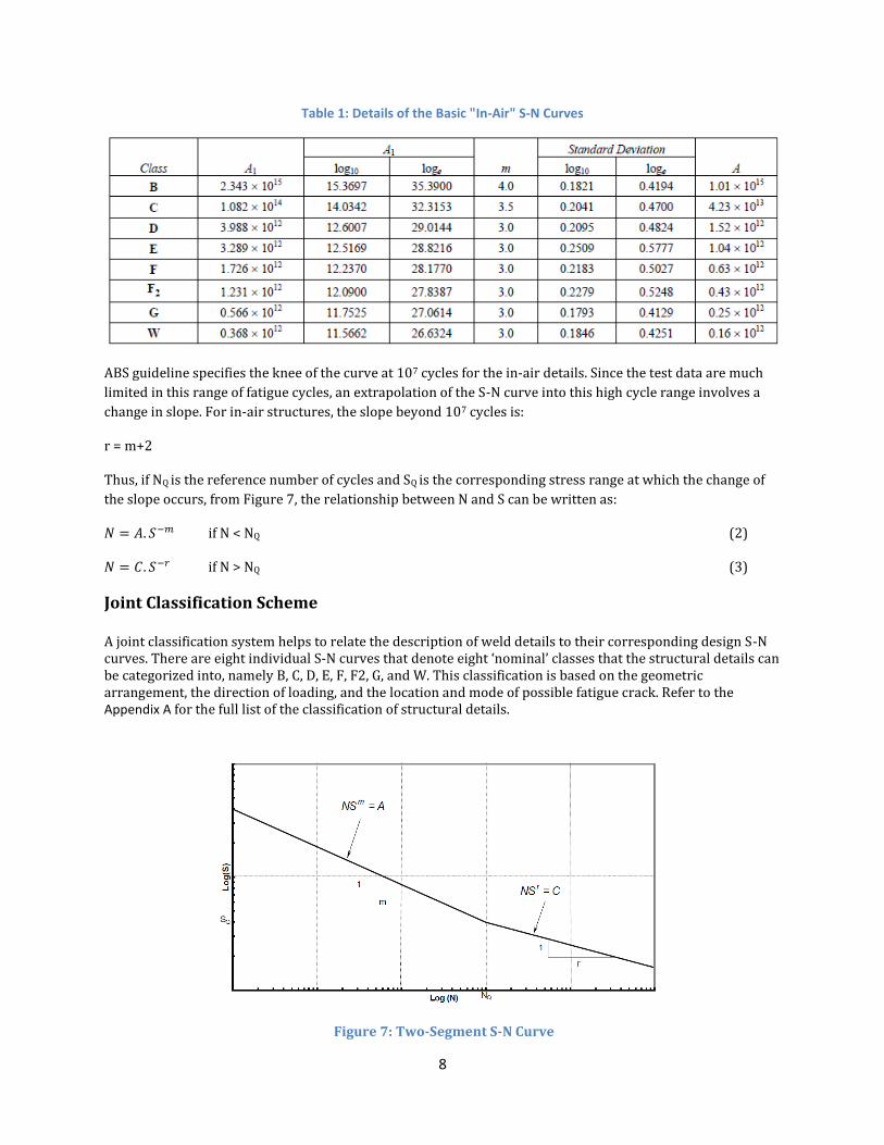
Table 1: Details of the Basic "In-Air" S-N Curves
ABS guideline specifies the knee of the curve at 107 cycles for the in-air details. Since the test data are much
limited in this range of fatigue cycles, an extrapolation of the S-N curve into this high cycle range involves a
change in slope. For in-air structures, the slope beyond 107 cycles is:
r = m+2
Thus, if NQ is the reference number of cycles and SQ is the corresponding stress range at which the change of
the slope occurs, from Figure 7, the relationship between N and S can be written as:
if N < NQ (2)
if N > NQ (3)
Joint Classification Scheme A joint classification system helps to relate the description of weld details to their corresponding design S-N curves. There are eight individual S-N curves that denote eight ‘nominal’ classes that the structural details can be categorized into, namely B, C, D, E, F, F2, G, and W. This classification is based on the geometric arrangement, the direction of loading, and the location and mode of possible fatigue crack. Refer to the Appendix A for the full list of the classification of structural details.
Figure 7: Two-Segment S-N Curve

9
Adjustment to the S-N Curves In general, the laboratory specimens that the S-N data are based on are considered different in geometry from the actual size of the structural component. Thus, some adjustments are needed to achieve the expected performance for actual structural details. In this regard, ABS identifies two major considerations that require special awareness and possible adjustment in the fatigue assessment process. These are the effect of thickness and the relative corrosiveness of the environment in which the structural detail is subjected to variable stress.
Scale or Thickness Effect
The fatigue performance of welded joints is dependent on the plate thickness to some extent. For the same
stress range, the detail’s fatigue strength, which cracks from the weld toe, decreases with the increase in plate
thickness. The stress concentration to greater depth in thick sections influence the cracks more than in thin
ones, thus the fatigue performance changes with the change in thickness of the structure. The size effect in
fatigue in which larger sections tend to be weaker is manifested in welded joint fatigue by a thickness
adjustment.
In ABS Guide, the basic design S-N curves are applicable to the structural components having thickness that
do not exceed the reference thickness (tR) of 22 mm. However, the adjustments are made to those with the
thickness above 22 mm. The ABS recommended thickness adjustment is based on studies of fatigue test data
and the models used by others.
The thickness effect is expressed by an adjustment formula:
(
) t > to (4)
t ≤ to (5)
Where,
Sf allowable stress range S allowable stress range from the nominal S-N design curve tR the reference thickness t0 thickness above which adjustments should be made t actual thickness A “thickness adjusted” S-N curve can be constructed when t > t0 and is of the form:
])([ q
Rt
tSmLogLogALogN (6)
Where, S unmodified stress range in the S-N curve tR reference thickness (= 22 mm) t plate thickness of the member under assessment q thickness exponent factor (= 0.25)
Hence, for plates thicker than 22 mm, ABS introduces the design stress penalty of (tref/t)0.25.
Environmental Condition/Corrosion Effect
Fatigue strength is reduced when the structure operates in a corrosive environment. The ABS
recommendations to take into account the influence of corrosion on fatigue strength are based on a review of
corrosion effects published in several guidance and other recommended documents in practice relating to
marine structures. Crack growth rates increase rapidly when the structures are corroded. To account for the
10
cathodic protection or the free corrosion conditions of the structures in the sea-water, the parameters for “In-
Air” curves are modified, and separate S-N curves are provided.
The parameters as given in the ABS Guidance on the Fatigue Assessment of the Offshore Structures, for the
‘In-Air’ (A) S-N curve, is given by Table 2.
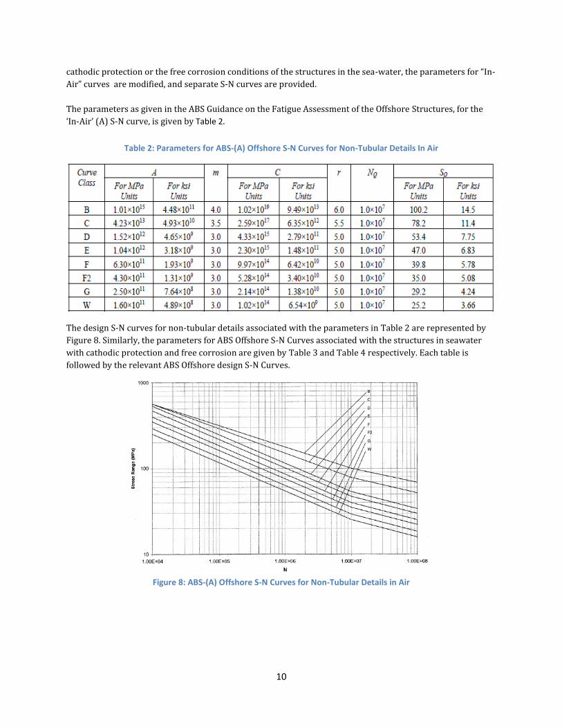
Table 2: Parameters for ABS-(A) Offshore S-N Curves for Non-Tubular Details In Air
The design S-N curves for non-tubular details associated with the parameters in Table 2 are represented by
Figure 8. Similarly, the parameters for ABS Offshore S-N Curves associated with the structures in seawater
with cathodic protection and free corrosion are given by Table 3 and Table 4 respectively. Each table is
followed by the relevant ABS Offshore design S-N Curves.
Figure 8: ABS-(A) Offshore S-N Curves for Non-Tubular Details in Air
11
Table 3: Parameters for ABS-(CP) Offshore S-N Curves for Non-Tubular Details in Seawater with Cathodic Protection
Figure 9: ABS-(CP) Offshore S-N Curves for Non-Tubular Details in Seawater with Cathodic Protection
Table 4: Parameters for ABS-(FC) Offshore S-N Curves for Non-Tubular Details in Seawater for Free Corrosion
12
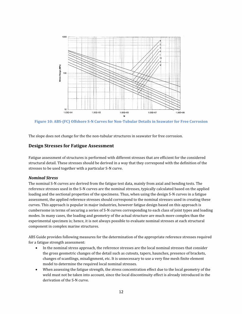
Figure 10: ABS-(FC) Offshore S-N Curves for Non-Tubular Details in Seawater for Free Corrosion
The slope does not change for the the non-tubular structures in seawater for free corrosion.
Design Stresses for Fatigue Assessment
Fatigue assessment of structures is performed with different stresses that are efficient for the considered
structural detail. These stresses should be derived in a way that they correspond with the definition of the
stresses to be used together with a particular S-N curve.
Nominal Stress
The nominal S-N curves are derived from the fatigue test data, mainly from axial and bending tests. The
reference stresses used in the S-N curves are the nominal stresses, typically calculated based on the applied
loading and the sectional properties of the specimens. Thus, when using the design S-N curves in a fatigue
assessment, the applied reference stresses should correspond to the nominal stresses used in creating these
curves. This approach is popular in major industries, however fatigue design based on this approach is
cumbersome in terms of securing a series of S-N curves corresponding to each class of joint types and loading
modes. In many cases, the loading and geometry of the actual structure are much more complex than the
experimental specimen is; hence, it is not always possible to evaluate nominal stresses at each structural
component in complex marine structures.
ABS Guide provides following measures for the determination of the appropriate reference stresses required
for a fatigue strength assessment:
In the nominal stress approach, the reference stresses are the local nominal stresses that consider
the gross geometric changes of the detail such as cutouts, tapers, haunches, presence of brackets,
changes of scantlings, misalignment, etc. It is unnecessary to use a very fine mesh finite element
model to determine the required local nominal stresses.
When assessing the fatigue strength, the stress concentration effect due to the local geometry of the
weld must not be taken into account, since the local discontinuity effect is already introduced in the
derivation of the S-N curve.
13
The principal stress adjacent to the potential crack locations should be utilized if the stress field is
more complex than a uniaxial field.
When the fatigue assessment of welded joints is performed, the welded attachment adds uncertainty about
the local stress and the applicable S-N curve at the weld locations. These are captured in the nominal stress
Joint Classification section. However, when the structure is complicated and too difficult to be classified, the
hot spot stress approach is implemented.
Hot-Spot Stress
Hot-Spot Stress approach, or geometric stress approach considers the increase in stress caused by the
configuration of the structural detail in consideration. It is applied to extract the stresses at the established
hot spot regions or already predicted high stresses areas. For the welded joints, hot spot location is at the
weld toe. The stress at the weld toe is calculated by a linear extrapolation of stresses over two reference
points in front of the considered weld toe.
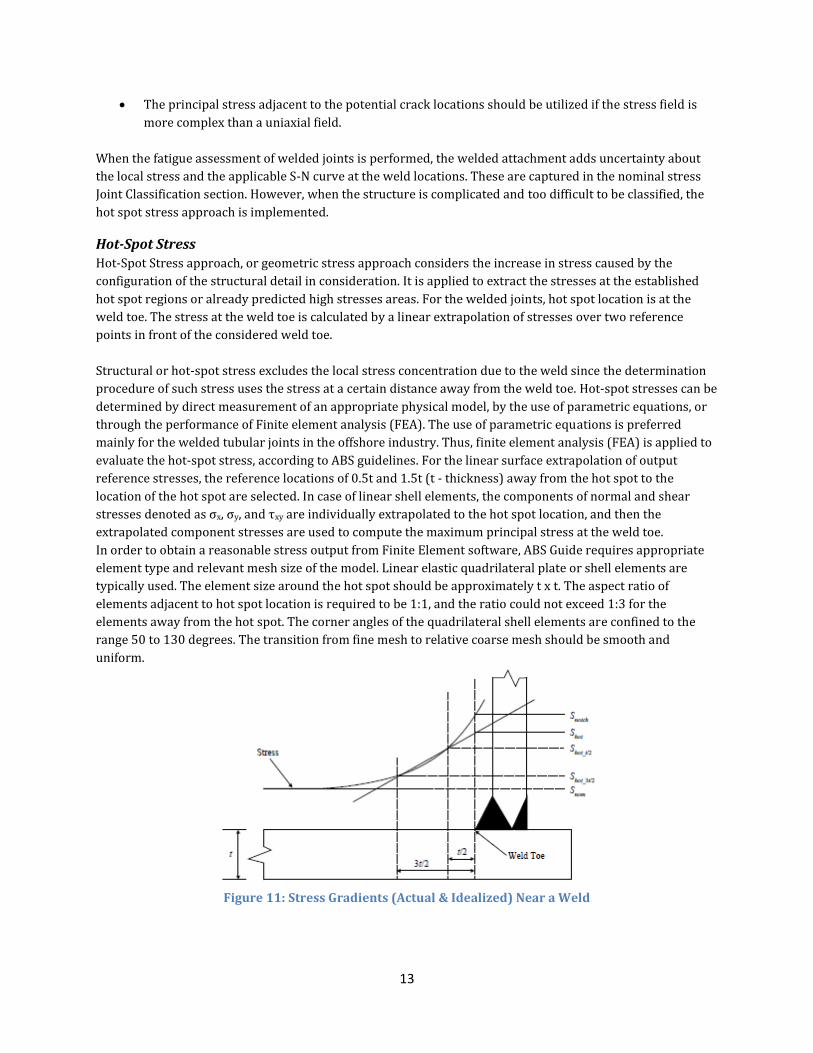
Structural or hot-spot stress excludes the local stress concentration due to the weld since the determination
procedure of such stress uses the stress at a certain distance away from the weld toe. Hot-spot stresses can be
determined by direct measurement of an appropriate physical model, by the use of parametric equations, or
through the performance of Finite element analysis (FEA). The use of parametric equations is preferred
mainly for the welded tubular joints in the offshore industry. Thus, finite element analysis (FEA) is applied to
evaluate the hot-spot stress, according to ABS guidelines. For the linear surface extrapolation of output
reference stresses, the reference locations of 0.5t and 1.5t (t - thickness) away from the hot spot to the
location of the hot spot are selected. In case of linear shell elements, the components of normal and shear
stresses denoted as σx, σy, and τxy are individually extrapolated to the hot spot location, and then the
extrapolated component stresses are used to compute the maximum principal stress at the weld toe.
In order to obtain a reasonable stress output from Finite Element software, ABS Guide requires appropriate
element type and relevant mesh size of the model. Linear elastic quadrilateral plate or shell elements are
typically used. The element size around the hot spot should be approximately t x t. The aspect ratio of
elements adjacent to hot spot location is required to be 1:1, and the ratio could not exceed 1:3 for the
elements away from the hot spot. The corner angles of the quadrilateral shell elements are confined to the
range 50 to 130 degrees. The transition from fine mesh to relative coarse mesh should be smooth and
uniform.
Figure 11: Stress Gradients (Actual & Idealized) Near a Weld
14
Assessment
Based on the literature review of ABS fatigue guidelines, following conclusion can be derived.
Stress definition is consistent and explicit when the nominal stress based S-N curves are adopted. However,
as previously mentioned it is extremely difficult to compute nominal stress for the structures with high level
of complexity in geometry as well as loading conditions. Therefore, ABS guideline resolves to the approach
like structural hot-spot stress method.
Hot-Spot stress approach reduces the number of eight S-N curves to one S-N curve, which is Class E.
Nonetheless, some drawbacks exist when using this approach. The derivation of the hot spot stress requires
finite element modeling, and it is sensitive to the element type and the mesh size and shape. There is no clear
justification to the reference locations, 0.5t and 1.5t, provided in ABS guide to extrapolate the surface stress.
Also, the adjustment formula to account for thickness effect calls for a specific reference thickness (tR) along
with the thickness exponent, q. The value of reference thickness is equal to 22 mm. The authors supposed
that the algorithm for the thickness adjustment formula was obtained using tubular joints, or perhaps using
some other procedure. The origin of the algorithm or the procedure to develop the thickness adjustment
formula is not well documented, and the reason for selection of the reference thickness is unclear. The value
of the thickness exponent provided is 0.25 for all curves. However, it is well known that not all joint types
have same effect with the change in thickness. For each class of curve, the rate of change of fatigue lives will
vary with the similar change in thickness. Thus, the constant value of this exponent is questionable.
Along with the scale and the environment effect, ABS guidelines is in agreement with the principle that was
established well over 30 years ago which concludes that the fatigue strength of the welded structures does
not increase with the increase in material strength. The crack propagation rate is not relevant to the material
tensile strength, unless the material is exposed to the corrosive environment. Furthermore, it is assumed that
a welded structure consist of the residual stress equal to the yield stress. Consequently, the fatigue life is
depended on the applied stress range rather than the mean stress, regardless of whether the stress is tensile
or compressive.
15
III. Test Procedures & Results
Introduction
Funded by the National Shipbuilding Research Program (NSRP) in 2011 and building on previous Office of
Naval Research (ONR) projects (Huang, et al. 2003 – 07), a joint project “Elimination of Overwelding to
Reduce Distortion in Naval Shipbuilding Applications” was initiated. HII-Ingalls and Applied Thermal Science
(ATS) fabricated welds to study their behavior through extensive tensile, static shear, fatigue, and dynamic
testing at four independent test sites including University of New Orleans (UNO), University of Maine
(UMaine), Naval Surface Warfare Center – Carderock Division (NSWCCD), and Concurrent Technologies
Corporation (CTC). This section focuses on the steel plate cruciform joints manufactured in order to evaluate
the fatigue strength of welded joints. The study provides fatigue test results for load-bearing and non-load-
bearing cruciform welded joints in 5 and 10 mm thick plates, which were tested at the University of New
Orleans. The test results are then compared to the current ABS fatigue design standards.
Test Method
Test Material
The test specimens were manufactured using 5 mm and 10 mm thick steel plates. They were cut and welded
at HII-Ingalls. The steel grades of ABS grade DH36 and HSLA-80 were used for several specimens to be tested;
whereas the rest of the specimens were of dissimilar strength, AH36 welded to HSLA-80, in order to reflect
weld details in actual ship structures. NSWCCD verified the material property of all base metal plates and the
metal weldments. The mechanical properties of these different materials are shown in the table below.
Table 5: Mechanical Properties of the Specimen Material
Material Yield Strength Ultimate Tensile Strength Elongation
AH 36 51000 psi 355 Mpa
71000 – 90000 psi 490 – 620 Mpa
21%
DH 36 51000 psi 355 Mpa
71000 – 90000 psi 490 – 620 Mpa
21%
HSLA 80 36000 – 86000 psi
250 – 590 Mpa 60000 – 95000 psi
414 – 655 Mpa
Test Specimen
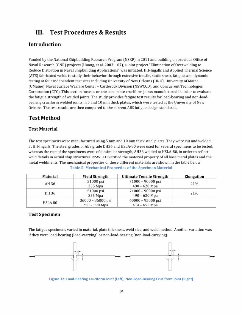
The fatigue specimens varied in material, plate thickness, weld size, and weld method. Another variation was
if they were load-bearing (load-carrying) or non-load-bearing (non-load-carrying).
Figure 12: Load-Bearing Cruciform Joint (Left); Non-Load-Bearing Cruciform Joint (Right)
16
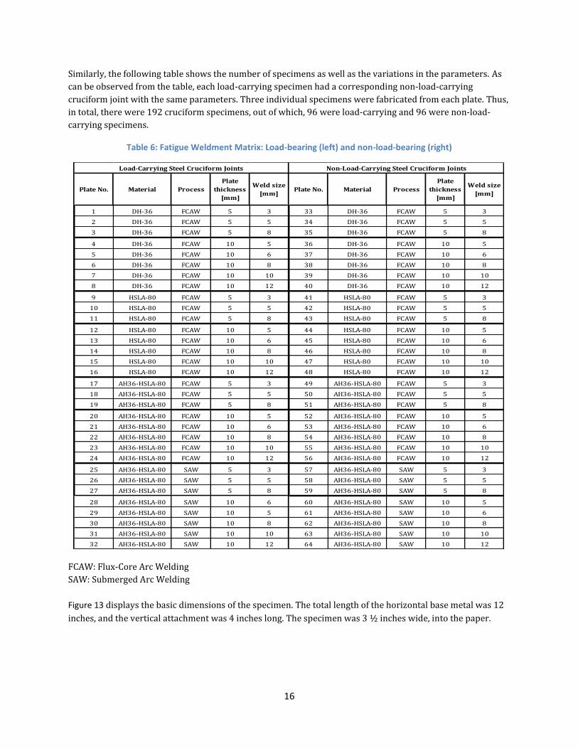
Similarly, the following table shows the number of specimens as well as the variations in the parameters. As
can be observed from the table, each load-carrying specimen had a corresponding non-load-carrying
cruciform joint with the same parameters. Three individual specimens were fabricated from each plate. Thus,
in total, there were 192 cruciform specimens, out of which, 96 were load-carrying and 96 were non-load-
carrying specimens.
Table 6: Fatigue Weldment Matrix: Load-bearing (left) and non-load-bearing (right)
FCAW: Flux-Core Arc Welding
SAW: Submerged Arc Welding
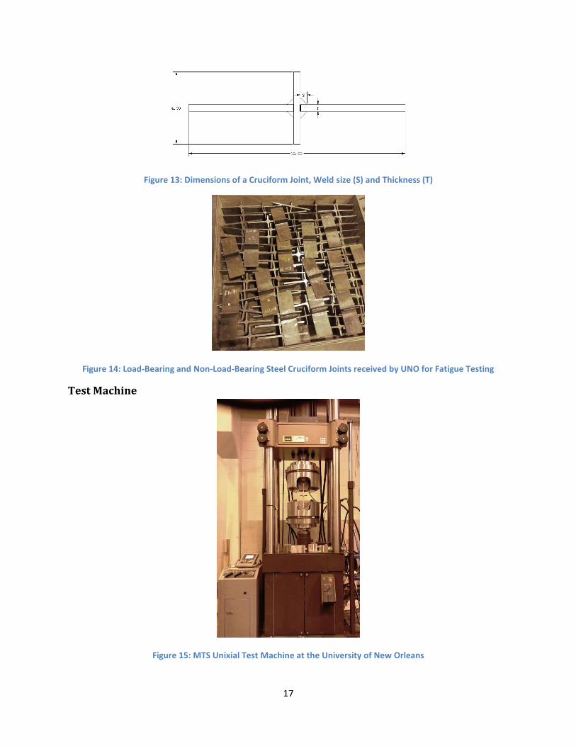
Figure 13 displays the basic dimensions of the specimen. The total length of the horizontal base metal was 12
inches, and the vertical attachment was 4 inches long. The specimen was 3 ½ inches wide, into the paper.
Plate No. Material Process
Plate
thickness
[mm]
Weld size
[mm]Plate No. Material Process
Plate
thickness
[mm]
Weld size
[mm]
1 DH-36 FCAW 5 3 33 DH-36 FCAW 5 3
2 DH-36 FCAW 5 5 34 DH-36 FCAW 5 5
3 DH-36 FCAW 5 8 35 DH-36 FCAW 5 8
4 DH-36 FCAW 10 5 36 DH-36 FCAW 10 5
5 DH-36 FCAW 10 6 37 DH-36 FCAW 10 6
6 DH-36 FCAW 10 8 38 DH-36 FCAW 10 8
7 DH-36 FCAW 10 10 39 DH-36 FCAW 10 10
8 DH-36 FCAW 10 12 40 DH-36 FCAW 10 12
9 HSLA-80 FCAW 5 3 41 HSLA-80 FCAW 5 3
10 HSLA-80 FCAW 5 5 42 HSLA-80 FCAW 5 5
11 HSLA-80 FCAW 5 8 43 HSLA-80 FCAW 5 8
12 HSLA-80 FCAW 10 5 44 HSLA-80 FCAW 10 5
13 HSLA-80 FCAW 10 6 45 HSLA-80 FCAW 10 6
14 HSLA-80 FCAW 10 8 46 HSLA-80 FCAW 10 8
15 HSLA-80 FCAW 10 10 47 HSLA-80 FCAW 10 10
16 HSLA-80 FCAW 10 12 48 HSLA-80 FCAW 10 12
17 AH36-HSLA-80 FCAW 5 3 49 AH36-HSLA-80 FCAW 5 3
18 AH36-HSLA-80 FCAW 5 5 50 AH36-HSLA-80 FCAW 5 5
19 AH36-HSLA-80 FCAW 5 8 51 AH36-HSLA-80 FCAW 5 8
20 AH36-HSLA-80 FCAW 10 5 52 AH36-HSLA-80 FCAW 10 5
21 AH36-HSLA-80 FCAW 10 6 53 AH36-HSLA-80 FCAW 10 6
22 AH36-HSLA-80 FCAW 10 8 54 AH36-HSLA-80 FCAW 10 8
23 AH36-HSLA-80 FCAW 10 10 55 AH36-HSLA-80 FCAW 10 10
24 AH36-HSLA-80 FCAW 10 12 56 AH36-HSLA-80 FCAW 10 12
25 AH36-HSLA-80 SAW 5 3 57 AH36-HSLA-80 SAW 5 3
26 AH36-HSLA-80 SAW 5 5 58 AH36-HSLA-80 SAW 5 5
27 AH36-HSLA-80 SAW 5 8 59 AH36-HSLA-80 SAW 5 8
28 AH36-HSLA-80 SAW 10 6 60 AH36-HSLA-80 SAW 10 5
29 AH36-HSLA-80 SAW 10 5 61 AH36-HSLA-80 SAW 10 6
30 AH36-HSLA-80 SAW 10 8 62 AH36-HSLA-80 SAW 10 8
31 AH36-HSLA-80 SAW 10 10 63 AH36-HSLA-80 SAW 10 10
32 AH36-HSLA-80 SAW 10 12 64 AH36-HSLA-80 SAW 10 12
Load-Carrying Steel Cruciform Joints Non-Load-Carrying Steel Cruciform Joints
17
Figure 13: Dimensions of a Cruciform Joint, Weld size (S) and Thickness (T)
Figure 14: Load-Bearing and Non-Load-Bearing Steel Cruciform Joints received by UNO for Fatigue Testing
Test Machine
Figure 15: MTS Unixial Test Machine at the University of New Orleans
18
In the laboratory of the University of New Orleans, the fatigue tests were conducted in an MTS uniaxial testing
machine where the specimens were loaded using hydraulic grips and cycled axially. The machine has a force
capacity of 200 kips and MTS 647 Hydraulic wedge grips with force capacity of 110 kips and maximum
operative pressure of 9,000 psi. Hydraulic wedge grips were used to mount the specimens, and to apply the
loads on them. Along with the grips, there are four individual (or two pairs of) wedges mounted on the grips.
These wedges are 3.5 inches deep, 3.75 inches wide, and opens from 0 to 10.9 mm. The metal brackets are
used to keep the specimens aligned in the center of the wedges. The machine operated remotely using
FlexTest GT software from which the load levels and frequencies were specified. 5” of gage length was
specified for all the 12” specimens to avoid any buckling during the test procedure.
Test Requirements
As per the specification by project sponsor, NSRP, fatigue testing was carried out in accordance with ASTM
E466 using gage length of 5 inches.
Load Specification
There were two stress ranges at R = -1 that were applied to the specimens: 30 ksi (+/-15ksi amplitude) and
60 ksi(+/-30 ksi amplitude). The table below specifies the number of specimens tested under the specified
loads.
Table 7: Load Specification for Test of Individual Cruciform Joint
Total Specimens
Fatigue test at stress range 30 ksi [207 MPa]
Fatigue test at stress range 60 ksi [414 MPa]
Spare specimens
Load Carrying 96 32 54 10 Non-load-carrying 96 32 54 10 R ratio = minimum load/maximum load = -1
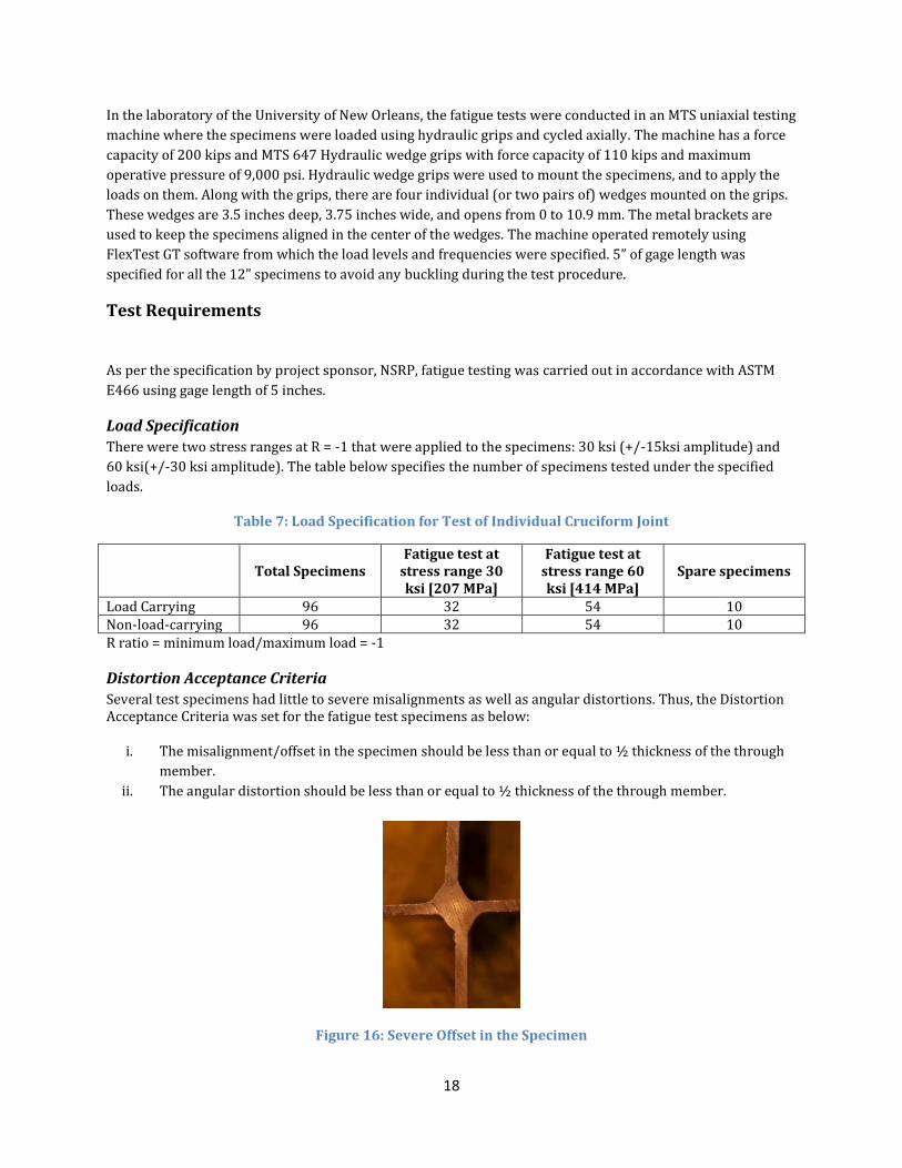
Distortion Acceptance Criteria
Several test specimens had little to severe misalignments as well as angular distortions. Thus, the Distortion Acceptance Criteria was set for the fatigue test specimens as below:
i. The misalignment/offset in the specimen should be less than or equal to ½ thickness of the through
member.
ii. The angular distortion should be less than or equal to ½ thickness of the through member.
Figure 16: Severe Offset in the Specimen
19
Failure Criteria
The elevation of cruciform joint’s compliance to 100% marked its failure. In other words, the fatigue failure
criteria set for all the specimens was at 50% reduction of the specimen stiffness.
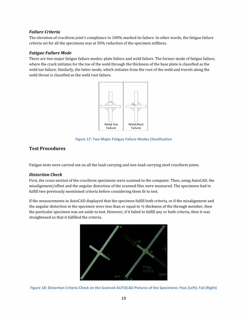
Fatigue Failure Mode There are two major fatigue failure modes: plate failure and weld failure. The former mode of fatigue failure,
where the crack initiates for the toe of the weld through the thickness of the base plate is classified as the
weld toe failure. Similarly, the latter mode, which initiates from the root of the weld and travels along the
weld throat is classified as the weld root failure.
Figure 17: Two Major Fatigue Failure Modes Classification
Test Procedures
Fatigue tests were carried out on all the load-carrying and non-load-carrying steel cruciform joints.
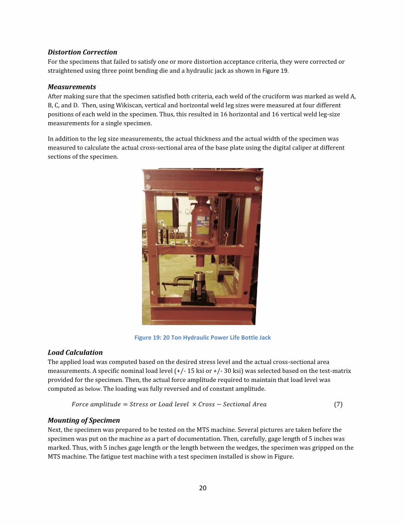
Distortion Check
First, the cross-section of the cruciform specimens were scanned to the computer. Then, using AutoCAD, the
misalignment/offset and the angular distortion of the scanned files were measured. The specimens had to
fulfill two previously mentioned criteria before considering them fit to test.
If the measurements in AutoCAD displayed that the specimen fulfill both criteria, or if the misalignment and
the angular distortion in the specimen were less than or equal to ½ thickness of the through member, then
the particular specimen was set aside to test. However, if it failed to fulfill any or both criteria, then it was
straightened so that it fulfilled the criteria.
Figure 18: Distortion Criteria Check on the Scanned AUTOCAD Pictures of the Specimens: Pass (Left); Fail (Right)
20
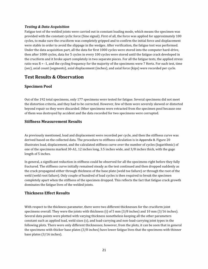
Distortion Correction
For the specimens that failed to satisfy one or more distortion acceptance criteria, they were corrected or
straightened using three point bending die and a hydraulic jack as shown in Figure 19.
Measurements
After making sure that the specimen satisfied both criteria, each weld of the cruciform was marked as weld A,
B, C, and D. Then, using Wikiscan, vertical and horizontal weld leg sizes were measured at four different
positions of each weld in the specimen. Thus, this resulted in 16 horizontal and 16 vertical weld leg-size
measurements for a single specimen.
In addition to the leg size measurements, the actual thickness and the actual width of the specimen was
measured to calculate the actual cross-sectional area of the base plate using the digital caliper at different
sections of the specimen.
Figure 19: 20 Ton Hydraulic Power Life Bottle Jack
Load Calculation The applied load was computed based on the desired stress level and the actual cross-sectional area
measurements. A specific nominal load level (+/- 15 ksi or +/- 30 ksi) was selected based on the test-matrix
provided for the specimen. Then, the actual force amplitude required to maintain that load level was
computed as below. The loading was fully reversed and of constant amplitude.
(7)
Mounting of Specimen Next, the specimen was prepared to be tested on the MTS machine. Several pictures are taken before the
specimen was put on the machine as a part of documentation. Then, carefully, gage length of 5 inches was
marked. Thus, with 5 inches gage length or the length between the wedges, the specimen was gripped on the
MTS machine. The fatigue test machine with a test specimen installed is show in Figure.
21
Testing & Data Acquisition
Fatigue test of the welded joints were carried out in constant loading mode, which means the specimen was
provided with the constant cyclic force (Sine signal). First of all, the force was applied for approximately 100
cycles, to make sure the cruciform was completely gripped and to confirm the initial force and displacement
were stable in order to avoid the slippage in the wedges. After verification, the fatigue test was performed.
Under the data acquisition part, all the data for first 1000 cycles were stored into the computer hard-drive,
then after 1000 cycles, data for 5 cycles in every 100 cycles were stored until the fatigue crack developed in
the cruciform and it broke apart completely in two separate pieces. For all the fatigue tests, the applied stress
ratio was R = -1, and the cycling frequency for the majority of the specimens were 7 Hertz. For each test, time
(sec), axial count (segments), axial displacement (inches), and axial force (kips) were recorded per cycle.
Test Results & Observation
Specimen Pool
Out of the 192 total specimens, only 177 specimens were tested for fatigue. Several specimens did not meet
the distortion criteria, and they had to be corrected. However, few of them were severely skewed or distorted
beyond repair so they were discarded. Other specimens were retracted from the specimen pool because one
of them was destroyed by accident and the data recorded for two specimens were corrupted.
Stiffness Measurement Results
As previously mentioned, load and displacement were recorded per cycle, and then the stiffness curve was
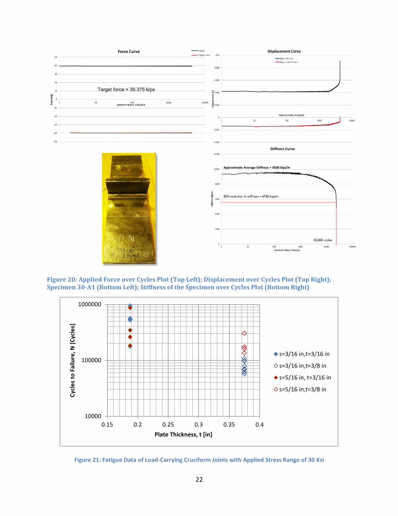
derived based on the collected data. The procedure to stiffness calculation is in Appendix B. Figure 20
illustrates load, displacement, and the calculated stiffness curve over the number of cycles (logarithmic) of
one of the specimens marked 30-A1, 12 inches long, 3.5 inches wide, and 3/8 inches thick, with the gage
length of 5 inches.
In general, a significant reduction in stiffness could be observed for all the specimens right before they fully
fractured. The stiffness curve initially remained steady as the test continued and then dropped suddenly as
the crack propagated either through thickness of the base plate (weld toe failure) or through the root of the
weld (weld root failure). Only couple of hundred of load cycles is then required to break the specimen
completely apart when the stiffness of the specimen dropped. This reflects the fact that fatigue crack growth
dominates the fatigue lives of the welded joints.
Thickness Effect Results
With respect to the thickness parameter, there were two different thicknesses for the cruciform joint
specimens overall. They were the joints with thickness (t) of 5 mm (3/8 inches) and 10 mm (3/16 inches).
Several data points were plotted with varying thickness nonetheless keeping all the other parameters
constant such as applied load, weld sizes (s), and load-carrying and non-load-carrying joint types in the
following plots. There were only different thicknesses; however, from the plots, it can be seen that in general
the specimens with thicker base plates (3/8 inches) have lower fatigue lives that the specimens with thinner
base plates (3/16 inches).
22
Figure 20: Applied Force over Cycles Plot (Top Left); Displacement over Cycles Plot (Top Right); Specimen 30-A1 (Bottom Left); Stiffness of the Specimen over Cycles Plot (Bottom Right)
Figure 21: Fatigue Data of Load-Carrying Cruciform Joints with Applied Stress Range of 30 Ksi
10000
100000
1000000
0.15 0.2 0.25 0.3 0.35 0.4
Cyc
les
to F
ailu
re, N
[C
ycle
s]
Plate Thickness, t [in]
s=3/16 in,t=3/16 in
s=3/16 in,t=3/8 in
s=5/16 in, t=3/16 in
s=5/16 in,t=3/8 in

23
Figure 22: Fatigue Data of Load-Carrying Cruciform Joints with Applied Stress Range of 60 Ksi
Figure 23: Fatigue Data of Non-Load-Carrying Cruciform Joints with Applied Stress Range of 30 Ksi
1,000
10,000
100,000
0.15 0.2 0.25 0.3 0.35 0.4
Cyc
les
to F
ailu
re, N
[C
ycle
s]
Plate Thickness, t [in]
s=5/16 in, t=3/16 in
s=5/16 in, t=3/8 in
s=3/16 in, t=3/16 in
s=3/16, t=3/8 in
80000
800000
8000000
0.15 0.2 0.25 0.3 0.35 0.4
Cyc
les
to F
ailu
re, N
[C
ycle
s]
Plate Thickness, t [in]
s=3/16 in,t=3/16 in
s=3/16 in,t=3/8 in
s=5/16 in, t=3/16 in
s=5/16 in,t=3/8 in
24
Figure 24: Fatigue Data of Non-Load-Carrying Cruciform Joints with Applied Stress Range of 60 Ksi
Fatigue Failure Path and the Critical Point
The observation of the fracture surfaces after the fatigue tests led to the identification of fatigue failure paths.
These failure paths were based on the initiation location of the cracks and their direction of the propagation.
i) Toe failure - The crack started at either side of the weld toe and the crack propagated through
thickness of the base metal plate. See Figure 25.
ii) Root failure - The crack initiated at the root of the weld and eventually travelled to the weld
surface. See Figure 26.
Besides, few specimens did not develop fatigue crack during the testing, even beyond 2 million cycles, thus,
the failure path could not be identified in those joints. Such joints were classified as the runout specimens.
Table 8: Number of Tested Joints and their Fatigue Failure Path
Cruciform Joint Type Toe Failure Root Failure Runouts Load-bearing 61 30 0
Non-load-bearing 80 0 6
As illustrated in Table 8, none of the non-load-bearing specimens experienced fatigue failure at the weld root;
whereas, both load-carrying and non-load-carrying specimens had weld toe failures. Furthermore, only the
non-load-carrying specimens had 6 runouts.
10000
100000
1000000
0.15 0.2 0.25 0.3 0.35 0.4
Cyc
les
to F
ailu
re, N
[C
ycle
s]
Plate Thickness, t [in]
s=3/16 in,t=3/16 in
s=3/16 in,t=3/8 in
s=5/16 in, t=3/16 in
s=5/16 in,t=3/8 in

25
Figure 25: Fatigue Failure Path: Weld Toe
Figure 26: Fatigue Failure Path: Weld Root or Weld Throat
In the marine industry standard, despite the inevitableness of fatigue failure, toe failure is usually preferred
to the root failures in the welded joints. The toe failures represent the crack in the base metal, which is
convenient to locate, and thus, corrective measures can be taken immediately in contrast to the weld root
failures where it is not possible to locate the fracture until the complete separation of the joint. Utilizing only
non-load-bearing type of structural detail will avoid the weld root failure issue; however, it is not viable at all.
Only for the load-bearing cruciform joints, the fatigue lives when plotted against the corresponding weld sizes
(s) normalized by base plate thicknesses (t), a specific marked point can be observed that divides internal
weld root failure from the external weld toe failure. Figure 27 shows the cycles to failure of the specimens
against the nominal s/t ratio (weld size to the plate thickness ratio) for both stress range levels of 30 ksi and
60 ksi.
26
Figure 27: Fatigue Life of Load-Carrying Joints Vs. Nominal s/t ratio, Critical Point
Replacing the nominal weld leg sizes with the actual weld leg sizes and the thicknesses of each specimen,
following plot, Figure 28, was generated, which is more justified. The plot clearly confirms that within the s/t
ratio region of about 0.75 to 0.95, both fatigue failure modes of weld toe failure and weld root failure exist.
However, when s/t ratio of the specimen is below the specified range, the crack occurs at the weld root, and
likewise, if s/t ratio of the specimen is beyond this range, the fatigue crack occurs at the weld toe.
Figure 28: Fatigue Life of Load-Carrying Joints Vs. Actual s/t ratio, Critical Point
1,000
10,000
100,000
1,000,000
0 0.2 0.4 0.6 0.8 1 1.2 1.4 1.6 1.8
N [
cycl
es]
Nominal s/t [-]
±15KSI Toe Failure
±15KSI Root Failure
±30KSI Toe Failure
±30KSI Root Failure
1,000
10,000
100,000
1,000,000
0 0.2 0.4 0.6 0.8 1 1.2 1.4 1.6 1.8 2
N [
cycl
es]
Actual s/t [-]
±15KSI Toe Failure
±15KSI Root Failure
±30KSI Toe Failure
±30KSI Root Failure
27
Therefore, on the contrary to popular belief that increasing weld size (or overwelding) on any structure
prevents the weld root failure, increase in weld size to base plate thickness ratio over 0.75 ≤ s/t ≤ 0.95 range
would rather confirm weld toe cracking in case of fatigue failure. Additionally, the fatigue cracks that
originated from the weld root seemed to have caused a significant reduction in the fatigue strength of the
welded joints as compared to the weld toe cracks.
Data Analysis & Discussions
Ultimately, the fatigue test results are utilized to estimate the fatigue life of the load-carrying and non-load-
carrying cruciform joints. The fatigue life evaluation of welded structures includes S-N data from actual
weldments in order to generate corresponding S-N plots. Thus, using the experimental results from the
fatigue test, experimental S-N plots were produced.
As identified previously, there are several uncertainties on how to determine the correct stresses at the weld
toe or root locations. Provided the time and scope of this project, only nominal stress approach was utilized in
order to generate the experimental S-N plots, and they were compared against ABS design S-N curves from its
Publication 115, Guide for The Fatigue Assessment of Offshore Structures.
Statistical Analysis
The correlation of the large database of fatigue test results in order to display a general trend of the data
requires a statistic regression analysis. Using the least squares fitting method, the statistical linear regression
analysis of the data was performed, and the standard deviation and the R-squared value was computed.
Standard deviation shows the variation of the dispersion of data points from the average or mean value of the
total data. It is non-dimensional in case of fatigue curves and represent the scatter of log(N), where “N” is the
number of cycles. The standard deviation for fatigue method is usually reported as 0.30, 0.40, 0.50, etc.
Essentially, well-correlated test data to the mean curve would have low standard deviation. Now, the
coefficient of determination or R-squared value provides a quantitative measure of the efficiency of the future
outcomes that are predicted by the model. The numerical value of R2 ranges from 0 to 1; the higher the R2
value, the better the regression line fits the data set.
The regression model is in the form: ( ) ( ); where N is the number of cycles to fatigue, S is
the applied stress, b0 is the intercept, and b1 is the inverse slope of the mean regression curve.
Nominal Stress Based Experimental S-N Chart
The load-carrying and non-load-carrying steel cruciform joints were tested with two different nominal stress
range levels, 30 ksi and 60 ksi. The S-N charts in the following figures: Figure 29, Figure 30, and Figure 31
exhibit the nominal stress range against the number of cycles to failure for each specimen.
The fatigue test results are presented in terms of nominal stress ranges. The solid lines in the plots are the
mean regression line to display the general trend of the data. The mean regression line represents the 50%
survival probability. The broken lines are the upper bound and the lower bound curves. The lower bound line
is calculated by subtracting two standard deviations of log N from solid line representing 95% survival
probability, whereas the upper bound line is calculated by adding two standard deviations of log N from the
solid line representing 5% survival probability.
28
In addition, the standard deviation (σ), R2 value, and the inverse slope of the plots (b1) are provided.
Figure 29: S-N Chart based on Nominal Stress Approach for Load-Carrying Steel Cruciform Joints
Figure 30: S-N Chart based on Nominal Stress Approach for Non-Load-Carrying Steel Cruciform Joints
100
1000
1000 10000 100000 1000000
No
min
al S
tre
ss R
ange
[M
Pa]
Cycles to Failure,N [Cycles]
Load-CarryingWeld Root FailureMean
Mean + 2σ
Mean - 2σ
Load-CarryingWeld Toe Failure
σ = 0.33 R2 = 0.70 b1 = -3.40
100
1000
10000 100000 1000000 10000000
No
min
al S
tre
ss R
ange
[M
Pa]
Cycles to Failure, N [Cycles]
Mean
Mean + 2σ
Mean - 2σ
Non-Load-Carrying
σ = 0.23 R2 = 0.77 b1 = -3.08
29
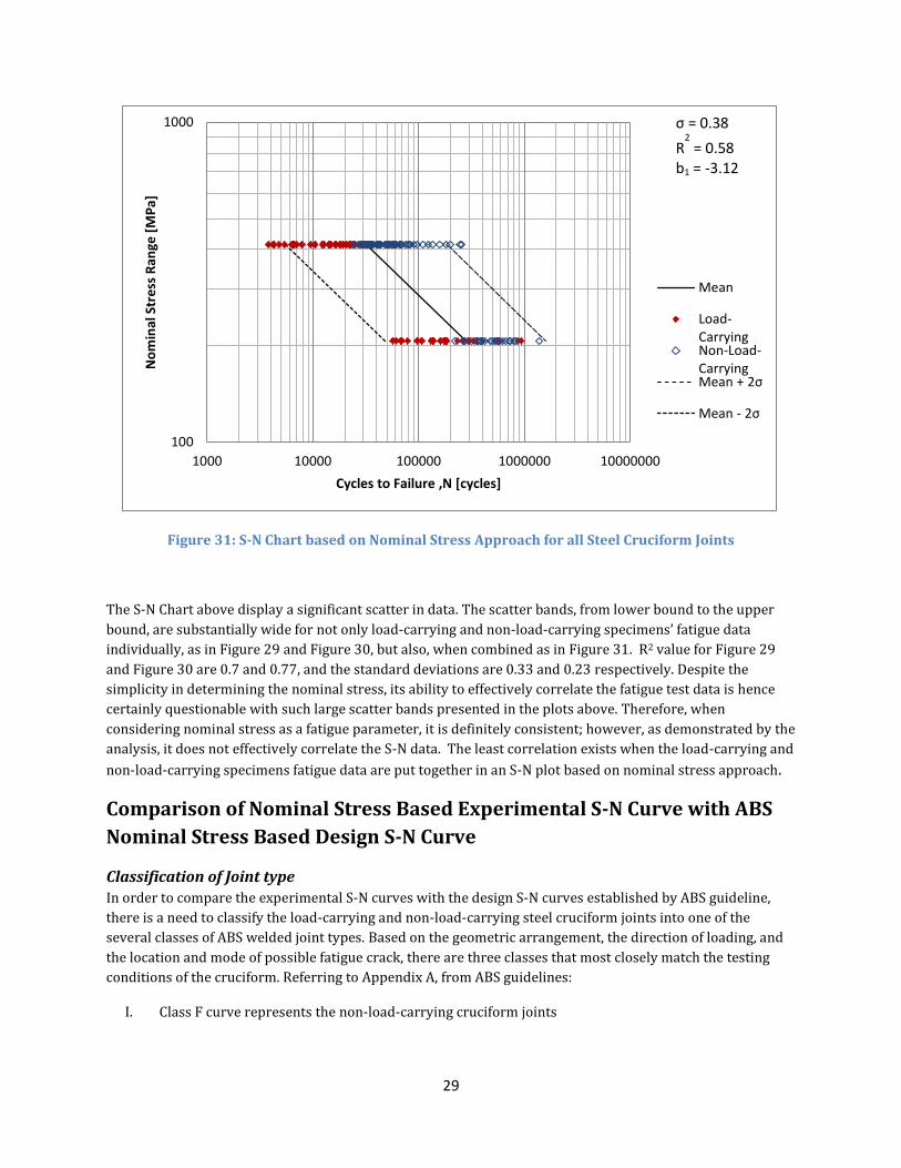
Figure 31: S-N Chart based on Nominal Stress Approach for all Steel Cruciform Joints
The S-N Chart above display a significant scatter in data. The scatter bands, from lower bound to the upper
bound, are substantially wide for not only load-carrying and non-load-carrying specimens’ fatigue data
individually, as in Figure 29 and Figure 30, but also, when combined as in Figure 31. R2 value for Figure 29
and Figure 30 are 0.7 and 0.77, and the standard deviations are 0.33 and 0.23 respectively. Despite the
simplicity in determining the nominal stress, its ability to effectively correlate the fatigue test data is hence
certainly questionable with such large scatter bands presented in the plots above. Therefore, when
considering nominal stress as a fatigue parameter, it is definitely consistent; however, as demonstrated by the
analysis, it does not effectively correlate the S-N data. The least correlation exists when the load-carrying and
non-load-carrying specimens fatigue data are put together in an S-N plot based on nominal stress approach.
Comparison of Nominal Stress Based Experimental S-N Curve with ABS
Nominal Stress Based Design S-N Curve
Classification of Joint type
In order to compare the experimental S-N curves with the design S-N curves established by ABS guideline,
there is a need to classify the load-carrying and non-load-carrying steel cruciform joints into one of the
several classes of ABS welded joint types. Based on the geometric arrangement, the direction of loading, and
the location and mode of possible fatigue crack, there are three classes that most closely match the testing
conditions of the cruciform. Referring to Appendix A, from ABS guidelines:
I. Class F curve represents the non-load-carrying cruciform joints
100
1000
1000 10000 100000 1000000 10000000
No
min
al S
tre
ss R
ange
[M
Pa]
Cycles to Failure ,N [cycles]
Mean
Load-CarryingNon-Load-CarryingMean + 2σ
Mean - 2σ
σ = 0.38
R2 = 0.58
b1 = -3.12
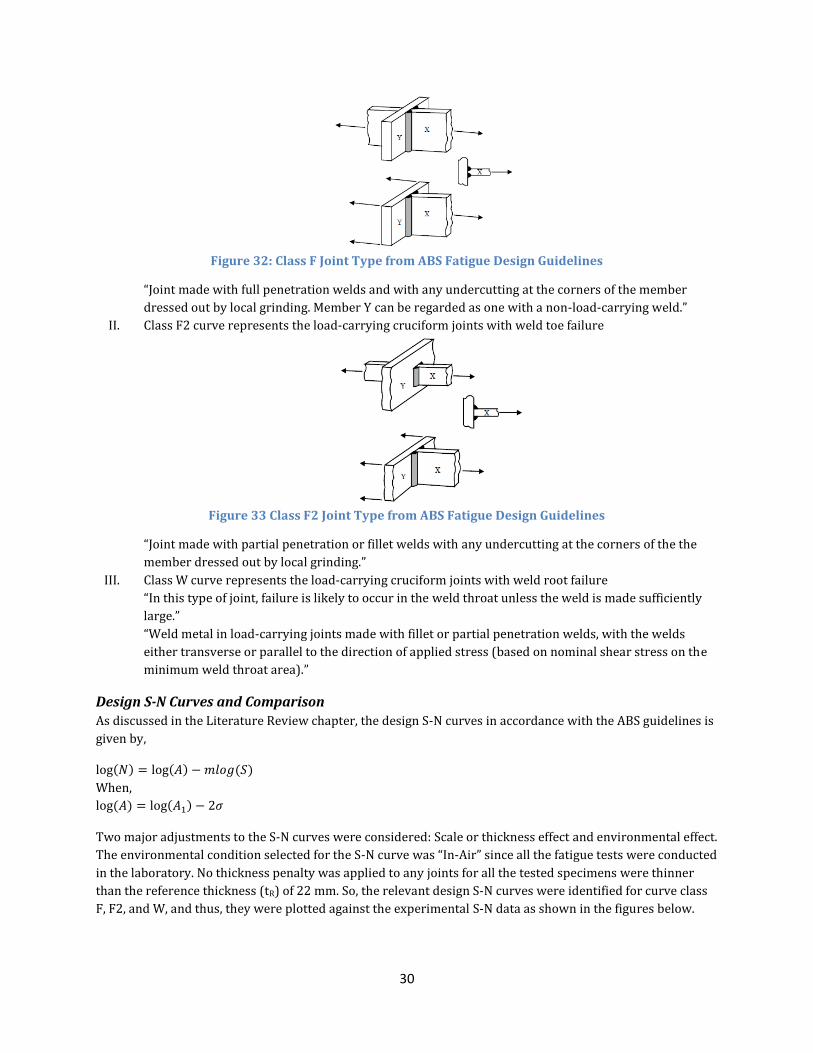
30
Figure 32: Class F Joint Type from ABS Fatigue Design Guidelines
“Joint made with full penetration welds and with any undercutting at the corners of the member
dressed out by local grinding. Member Y can be regarded as one with a non-load-carrying weld.”
II. Class F2 curve represents the load-carrying cruciform joints with weld toe failure
Figure 33 Class F2 Joint Type from ABS Fatigue Design Guidelines
“Joint made with partial penetration or fillet welds with any undercutting at the corners of the the
member dressed out by local grinding.”
III. Class W curve represents the load-carrying cruciform joints with weld root failure
“In this type of joint, failure is likely to occur in the weld throat unless the weld is made sufficiently
large.”
“Weld metal in load-carrying joints made with fillet or partial penetration welds, with the welds
either transverse or parallel to the direction of applied stress (based on nominal shear stress on the
minimum weld throat area).”
Design S-N Curves and Comparison
As discussed in the Literature Review chapter, the design S-N curves in accordance with the ABS guidelines is
given by,
( ) ( ) ( )
When,
( ) ( )
Two major adjustments to the S-N curves were considered: Scale or thickness effect and environmental effect.
The environmental condition selected for the S-N curve was “In-Air” since all the fatigue tests were conducted
in the laboratory. No thickness penalty was applied to any joints for all the tested specimens were thinner
than the reference thickness (tR) of 22 mm. So, the relevant design S-N curves were identified for curve class
F, F2, and W, and thus, they were plotted against the experimental S-N data as shown in the figures below.
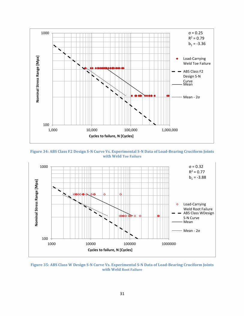
31
Figure 34: ABS Class F2 Design S-N Curve Vs. Experimental S-N Data of Load-Bearing Cruciform Joints with Weld Toe Failure
Figure 35: ABS Class W Design S-N Curve Vs. Experimental S-N Data of Load-Bearing Cruciform Joints with Weld Root Failure
100
1000
1,000 10,000 100,000 1,000,000
No
min
al S
tre
ss R
ange
[M
pa]
Cycles to failure, N [Cycles]
Load-CarryingWeld Toe Failure
ABS Class F2Design S-NCurveMean
Mean - 2σ
σ = 0.25 R2 = 0.79 b1 = -3.36
100
1000
1000 10000 100000 1000000
No
min
al S
tre
ss R
ange
[M
pa]
Cycles to failure, N [Cycles]
Load-CarryingWeld Root FailureABS Class WDesignS-N CurveMean
Mean - 2σ
σ = 0.32 R2 = 0.77 b1 = -3.88
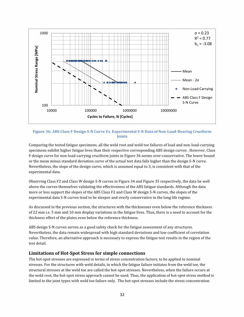
32
Figure 36: ABS Class F Design S-N Curve Vs. Experimental S-N Data of Non-Load-Bearing Cruciform Joints
Comparing the tested fatigue specimens, all the weld root and weld toe failures of load and non-load-carrying
specimens exhibit higher fatigue lives than their respective corresponding ABS design curves . However, Class
F design curve for non-load-carrying cruciform joints in Figure 36 seems over-conservative. The lower bound
or the mean minus standard deviation curve of the actual test data falls higher than the design S-N curve.
Nevertheless, the slope of the design curve, which is assumed equal to 3, is consistent with that of the
experimental data.
Observing Class F2 and Class W design S-N curves in Figure 34 and Figure 35 respectively, the data lie well
above the curves themselves validating the effectiveness of the ABS fatigue standards. Although the data
more or less support the slopes of the ABS Class F2 and Class W design S-N curves, the slopes of the
experimental data S-N curves tend to be steeper and overly conservative in the long life regime.
As discussed in the previous section, the structures with the thicknesses even below the reference thickness
of 22 mm i.e. 5 mm and 10 mm display variations in the fatigue lives. Thus, there is a need to account for the
thickness effect of the plates even below the reference thickness.
ABS design S-N curves serves as a good safety check for the fatigue assessment of any structures.
Nevertheless, the data remain widespread with high standard deviations and low coefficient of correlation
value. Therefore, an alternative approach is necessary to express the fatigue test results in the region of the
test detail.
Limitations of Hot-Spot Stress for simple connections The hot-spot stresses are expressed in terms of stress concentration factors, to be applied to nominal
stresses. For the structures with weld details, in which the fatigue failure initiates from the weld toe, the
structural stresses at the weld toe are called the hot-spot stresses. Nevertheless, when the failure occurs at
the weld root, the hot-spot stress approach cannot be used. Thus, the application of hot-spot stress method is
limited to the joint types with weld toe failure only. The hot-spot stresses include the stress concentration
100
1000
10000 100000 1000000 10000000
No
min
al S
tre
ss R
ange
[M
Pa]
Cycles to Failure, N [Cycles]
Mean
Mean - 2σ
Non-Load-Carrying
ABS Class F DesignS-N Curve
σ = 0.23 R2 = 0.77 b1 = -3.08
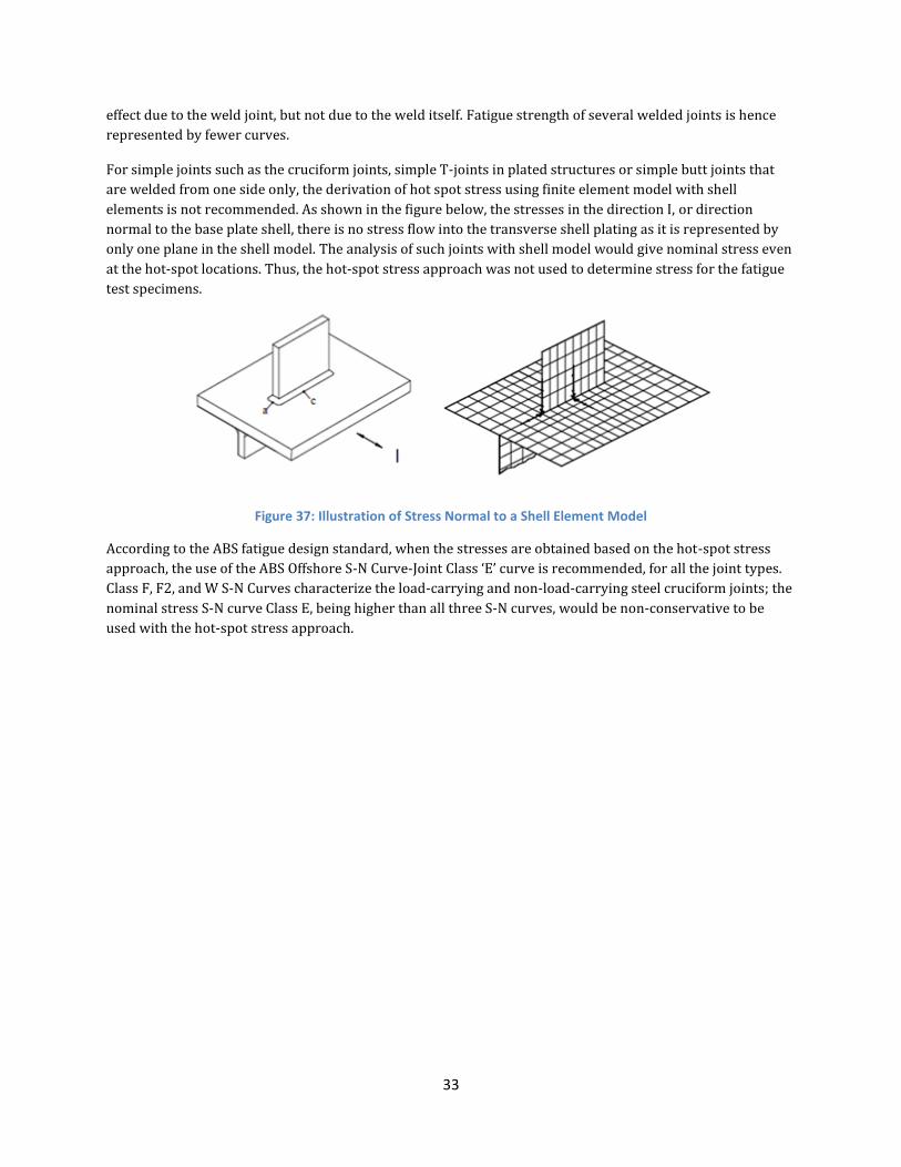
33
effect due to the weld joint, but not due to the weld itself. Fatigue strength of several welded joints is hence
represented by fewer curves.
For simple joints such as the cruciform joints, simple T-joints in plated structures or simple butt joints that
are welded from one side only, the derivation of hot spot stress using finite element model with shell
elements is not recommended. As shown in the figure below, the stresses in the direction I, or direction
normal to the base plate shell, there is no stress flow into the transverse shell plating as it is represented by
only one plane in the shell model. The analysis of such joints with shell model would give nominal stress even
at the hot-spot locations. Thus, the hot-spot stress approach was not used to determine stress for the fatigue
test specimens.
Figure 37: Illustration of Stress Normal to a Shell Element Model
According to the ABS fatigue design standard, when the stresses are obtained based on the hot-spot stress
approach, the use of the ABS Offshore S-N Curve-Joint Class ‘E’ curve is recommended, for all the joint types.
Class F, F2, and W S-N Curves characterize the load-carrying and non-load-carrying steel cruciform joints; the
nominal stress S-N curve Class E, being higher than all three S-N curves, would be non-conservative to be
used with the hot-spot stress approach.
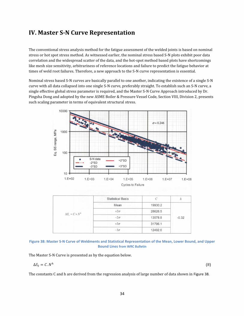
34
IV. Master S-N Curve Representation
The conventional stress analysis method for the fatigue assessment of the welded joints is based on nominal
stress or hot spot stress method. As witnessed earlier, the nominal stress based S-N plots exhibit poor data
correlation and the widespread scatter of the data, and the hot-spot method based plots have shortcomings
like mesh size sensitivity, arbitrariness of reference locations and failure to predict the fatigue behavior at
times of weld root failures. Therefore, a new approach to the S-N curve representation is essential.
Nominal stress based S-N curves are basically parallel to one another, indicating the existence of a single S-N
curve with all data collapsed into one single S-N curve, preferably straight. To establish such an S-N curve, a
single effective global stress parameter is required, and the Master S-N Curve Approach introduced by Dr.
Pingsha Dong and adopted by the new ASME Boiler & Pressure Vessel Code, Section VIII, Division 2, presents
such scaling parameter in terms of equivalent structural stress.
Figure 38: Master S-N Curve of Weldments and Statistical Representation of the Mean, Lower Bound, and Upper Bound Lines from WRC Bulletin
The Master S-N Curve is presented as by the equation below.
(8)
The constants C and h are derived from the regression analysis of large number of data shown in Figure 38.

35
Equivalent Structural Stress Parameter
The equivalent structural stress parameter is an effective global stress parameter, which is used as a basis to
establish Master S-N Curve. It is represented by the following equation:
( )
(9)
The equivalent structural stress parameter ( ) is obtained by normalizing the structural stress range ( ),
with two variable parameters, thickness (t) and the bending ratio (r) with m = 3.6, which is the value based
on fracture mechanics concept. As a result, it explicitly captures three major aspects of the fatigue behavior in
the welded joints that have been the topic of investigation.
i. Structural stress range ( ) captures the stress concentration effects of different joint types.
ii. The thickness correction term
provides the scale or effective plate thickness (t) effects.
iii. The bending ratio term, or the loading mode function ( )
captures the loading mode effects.
For the fatigue evaluations of welded joints, it is essential to observe the stress distribution at the fatigue
prone locations rather than a stress value at a single point. When the crack travels or propagates, the stress
alternates accordingly, hence the necessity of observing the stress distribution. The stress distribution at the
fatigue failure location, such as weld toe is represented by two stress states simultaneously: an equilibrium-
equivalent stress state and self-equilibrium stress state, as shown in figure below.
Figure 39: Through-thickness Structural Stresses Definition: Local Stresses, Structural Stress, and Self-Equilibrating Stress
Based on the fracture mechanics concept, the equilibrium-equivalent stress state or the traction-based stress
state signifies a stress state that is similar to the corresponding equivalent far field stress state. While the self-

36
equilibrating stress state represents the stress state influenced by the local notch geometry. This stress is
only dominant within a distance of 0.1t from the notch root. The thickness term and the bending ratio term
then consider the self-equilibrating notch stress effect aspect in the Master S-N Curve.
Traction-Based Structural Stress
The traction-based structural stress definition is based on the elementary structural mechanics theory. It is a
generalized nominal stress state at the fatigue prone location. Following considerations are made for the
fatigue evaluations of the welded joints:
a. Since the local effects due to the weld geometry is already captured in S-N data, a global based stress
measure is needed to exhibit the overall joint geometry effect along with the loading mode effect on
overall stress concentration. Based on elementary structural mechanics principles, such parameter
that captures the through-thickness distribution of stress state is in the form of membrane and
bending stress. Membrane stress (σm) represents the uniform stress through the thickness whereas
the bending stress (σb) represents the linear stress gradient in the stress state, as can be seen in
Figure 39.
b. Three structural stress components are relevant to fatigue crack, corresponding to the linear
representations of three traction components, along a hypothetical crack plane such as weld toe
cracking. They are normal, in-plane shear, and transverse shear stresses, and the membrane and
bending representation of these components satisfy the equilibrium conditions across and along the
crack plane. See Figure 40.
Figure 40: Exposing Three Structural Stress Components in Section A-A in a 2D Cross-Section (Left) and Section A-A-C-C in a 3D Cross-Section (Right)
c. The membrane and bending stresses are related to the line forces and the line moments. In FE
analysis, the line forces and moments relate to nodal forces and moments according to the nodal
force and displacement relationship. Displacement satisfies continuity in FE methods, thus the nodal
forces as well. In the displacement based FE procedures, the nodal forces and displacements are
considered to be the most fundamental quantities. The equilibrium conditions can be confirmed at
the nodes only in terms of nodal forces, not in terms of stresses.
Therefore, the traction-based structural stress is based on the reaction forces at the nodes. It is determined
using the nodal forces and moments along the hypothetical crack at the possible fatigue crack location,
satisfying the equilibrium conditions.
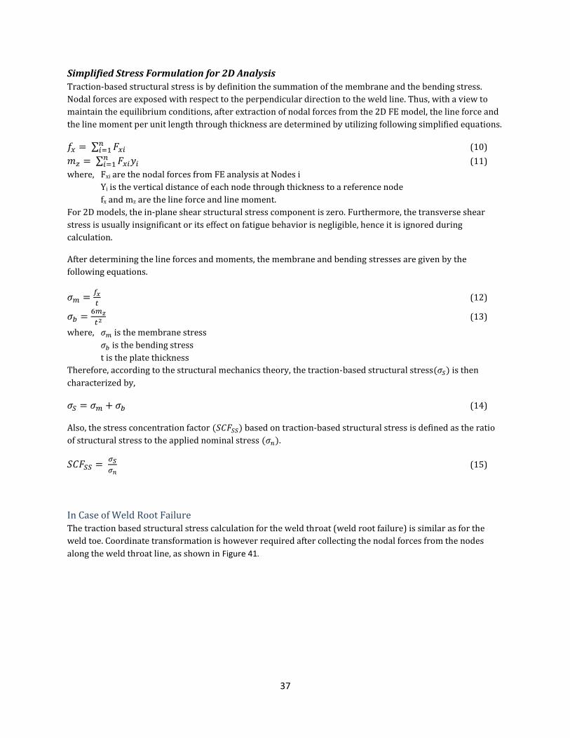
37
Simplified Stress Formulation for 2D Analysis
Traction-based structural stress is by definition the summation of the membrane and the bending stress.
Nodal forces are exposed with respect to the perpendicular direction to the weld line. Thus, with a view to
maintain the equilibrium conditions, after extraction of nodal forces from the 2D FE model, the line force and
the line moment per unit length through thickness are determined by utilizing following simplified equations.
∑ (10)
∑ (11)
where, Fxi are the nodal forces from FE analysis at Nodes i
Yi is the vertical distance of each node through thickness to a reference node
fx and mz are the line force and line moment.
For 2D models, the in-plane shear structural stress component is zero. Furthermore, the transverse shear
stress is usually insignificant or its effect on fatigue behavior is negligible, hence it is ignored during
calculation.
After determining the line forces and moments, the membrane and bending stresses are given by the
following equations.
(12)
(13)
where, is the membrane stress
is the bending stress
t is the plate thickness
Therefore, according to the structural mechanics theory, the traction-based structural stress( ) is then
characterized by,
(14)
Also, the stress concentration factor ( ) based on traction-based structural stress is defined as the ratio
of structural stress to the applied nominal stress ( ).
(15)
In Case of Weld Root Failure The traction based structural stress calculation for the weld throat (weld root failure) is similar as for the
weld toe. Coordinate transformation is however required after collecting the nodal forces from the nodes
along the weld throat line, as shown in Figure 41.
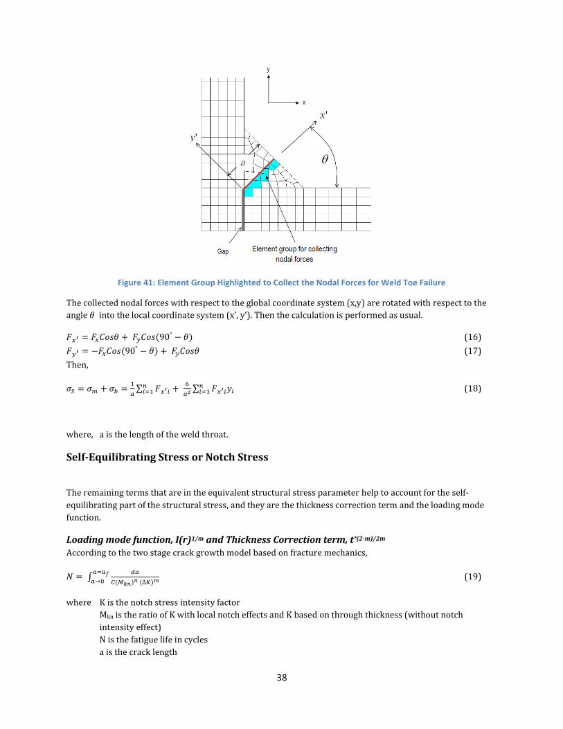
38
Figure 41: Element Group Highlighted to Collect the Nodal Forces for Weld Toe Failure
The collected nodal forces with respect to the global coordinate system (x,y) are rotated with respect to the
angle into the local coordinate system (x’, y’). Then the calculation is performed as usual.
( ) (16)
( ) (17)
Then,
∑
∑
(18)
where, a is the length of the weld throat.
Self-Equilibrating Stress or Notch Stress
The remaining terms that are in the equivalent structural stress parameter help to account for the self-
equilibrating part of the structural stress, and they are the thickness correction term and the loading mode
function.
Loading mode function, I(r)1/m and Thickness Correction term, t*(2-m)/2m
According to the two stage crack growth model based on fracture mechanics,
∫
( ) ( )
(19)
where K is the notch stress intensity factor
Mkn is the ratio of K with local notch effects and K based on through thickness (without notch
intensity effect)
N is the fatigue life in cycles
a is the crack length
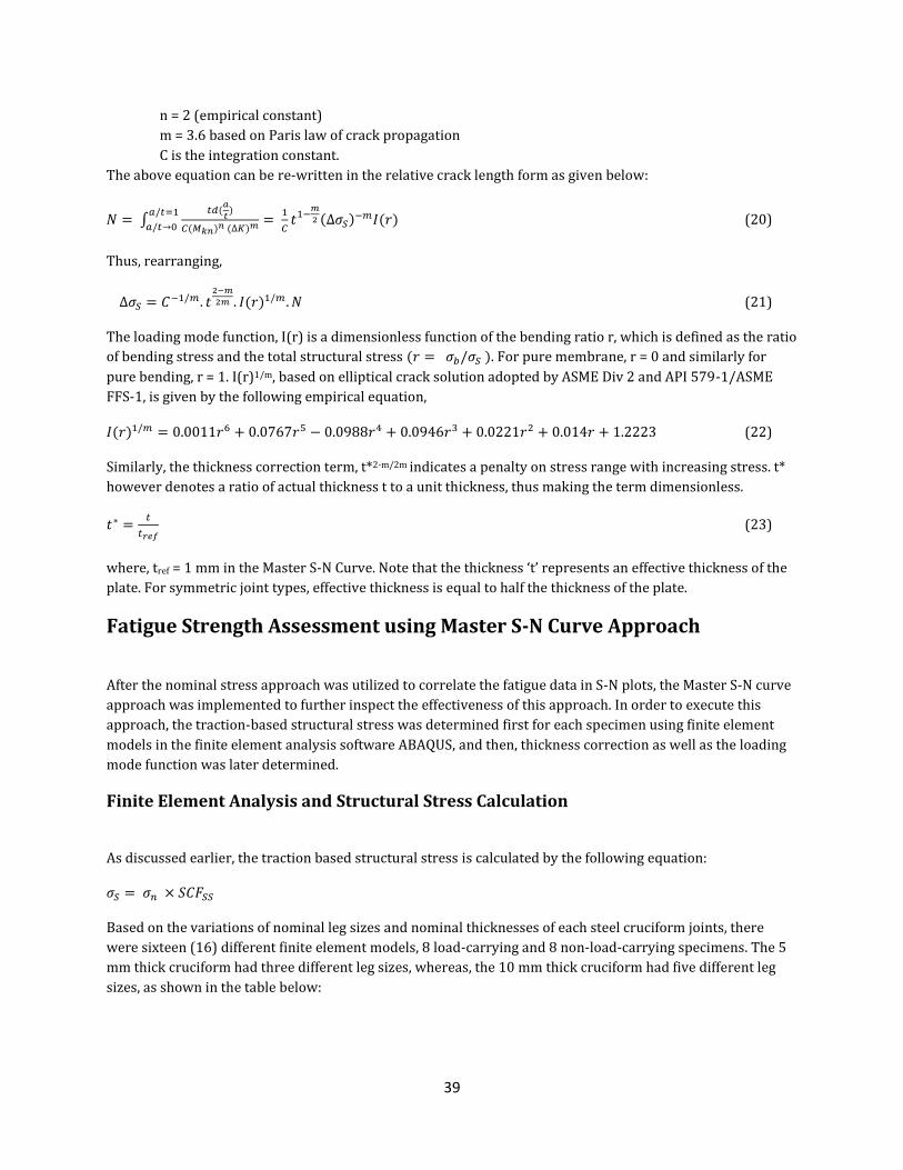
39
n = 2 (empirical constant)
m = 3.6 based on Paris law of crack propagation
C is the integration constant.
The above equation can be re-written in the relative crack length form as given below:
∫ (
)
( ) ( )
( ) ( )
(20)
Thus, rearranging,
( ) (21)
The loading mode function, I(r) is a dimensionless function of the bending ratio r, which is defined as the ratio
of bending stress and the total structural stress ( ). For pure membrane, r = 0 and similarly for
pure bending, r = 1. I(r)1/m, based on elliptical crack solution adopted by ASME Div 2 and API 579-1/ASME
FFS-1, is given by the following empirical equation,
( ) (22)
Similarly, the thickness correction term, t*2-m/2m indicates a penalty on stress range with increasing stress. t*
however denotes a ratio of actual thickness t to a unit thickness, thus making the term dimensionless.
(23)
where, tref = 1 mm in the Master S-N Curve. Note that the thickness ‘t’ represents an effective thickness of the
plate. For symmetric joint types, effective thickness is equal to half the thickness of the plate.
Fatigue Strength Assessment using Master S-N Curve Approach
After the nominal stress approach was utilized to correlate the fatigue data in S-N plots, the Master S-N curve
approach was implemented to further inspect the effectiveness of this approach. In order to execute this
approach, the traction-based structural stress was determined first for each specimen using finite element
models in the finite element analysis software ABAQUS, and then, thickness correction as well as the loading
mode function was later determined.
Finite Element Analysis and Structural Stress Calculation
As discussed earlier, the traction based structural stress is calculated by the following equation:
Based on the variations of nominal leg sizes and nominal thicknesses of each steel cruciform joints, there
were sixteen (16) different finite element models, 8 load-carrying and 8 non-load-carrying specimens. The 5
mm thick cruciform had three different leg sizes, whereas, the 10 mm thick cruciform had five different leg
sizes, as shown in the table below:
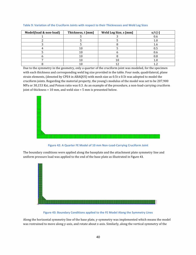
40
Table 9: Variation of the Cruciform Joints with respect to their Thicknesses and Weld Leg Sizes
Model(load & non-load) Thickness, t [mm] Weld Leg Size, s [mm] s/t [-] 1 5 3 0.6 2 5 5 1.0 3 5 8 1.6 4 10 5 0.5 5 10 6 0.6 6 10 8 0.8 7 10 10 1.0 8 10 12 1.2
Due to the symmetry in the geometry, only a quarter of the cruciform joint was modeled, for the specimen
with each thickness and corresponding weld leg size provided in the table. Four node, quadrilateral, plane
strain elements, (denoted by CPE4 in ABAQUS) with mesh size as 0.5t x 0.5t was adopted to model the
cruciform joints. Regarding the material property, the young’s modulus of the model was set to be 207,900
MPa or 30,153 Ksi, and Poison ratio was 0.3. As an example of the procedure, a non-load-carrying cruciform
joint of thickness = 10 mm, and weld size = 5 mm is presented below.
Figure 42: A Quarter FE Model of 10 mm Non-Load-Carrying Cruciform Joint
The boundary conditions were applied along the baseplate and the attachment plate symmetry line and
uniform pressure load was applied to the end of the base plate as illustrated in Figure 43.
Figure 43: Boundary Conditions applied to the FE Model Along the Symmetry Lines
Along the horizontal symmetry line of the base plate, y-symmetry was implemented which means the model
was restrained to move along y-axis, and rotate about z-axis. Similarly, along the vertical symmetry of the
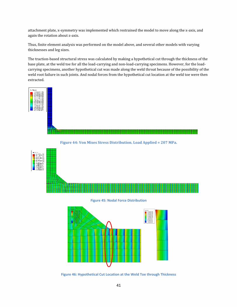
41
attachment plate, x-symmetry was implemented which restrained the model to move along the x-axis, and
again the rotation about z-axis.
Thus, finite element analysis was performed on the model above, and several other models with varying
thicknesses and leg sizes.
The traction-based structural stress was calculated by making a hypothetical cut through the thickness of the
base plate, at the weld toe for all the load-carrying and non-load-carrying specimens. However, for the load-
carrying specimens, another hypothetical cut was made along the weld throat because of the possibility of the
weld root failure in such joints. And nodal forces from the hypothetical cut location at the weld toe were then
extracted.
Figure 44: Von Mises Stress Distribution. Load Applied = 207 MPa.
Figure 45: Nodal Force Distribution
Figure 46: Hypothetical Cut Location at the Weld Toe through Thickness
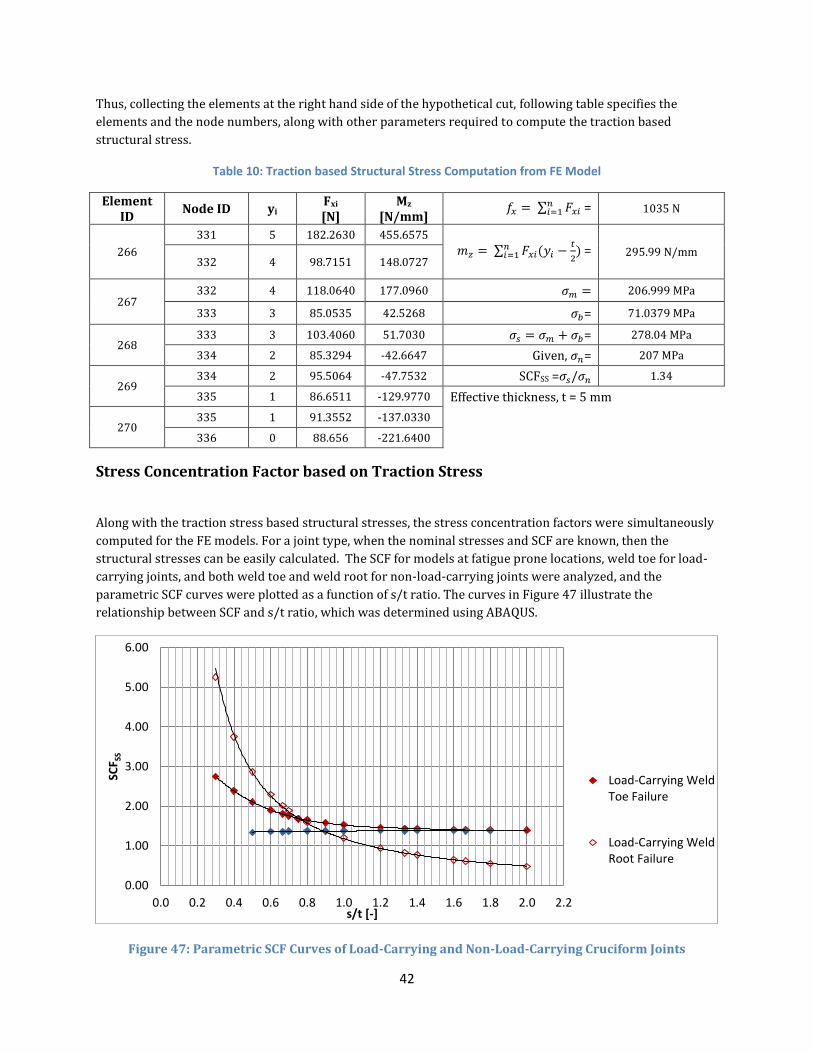
42
Thus, collecting the elements at the right hand side of the hypothetical cut, following table specifies the
elements and the node numbers, along with other parameters required to compute the traction based
structural stress.
Table 10: Traction based Structural Stress Computation from FE Model
Element ID
Node ID yi Fxi
[N] Mz
[N/mm] ∑
= 1035 N
266
331 5 182.2630 455.6575
∑ (
)
= 295.99 N/mm 332 4 98.7151 148.0727
267 332 4 118.0640 177.0960 206.999 MPa
333 3 85.0535 42.5268 = 71.0379 MPa
268 333 3 103.4060 51.7030 = 278.04 MPa
334 2 85.3294 -42.6647 Given, = 207 MPa
269 334 2 95.5064 -47.7532 SCFSS = 1.34
335 1 86.6511 -129.9770 Effective thickness, t = 5 mm
270 335 1 91.3552 -137.0330
336 0 88.656 -221.6400
Stress Concentration Factor based on Traction Stress
Along with the traction stress based structural stresses, the stress concentration factors were simultaneously
computed for the FE models. For a joint type, when the nominal stresses and SCF are known, then the
structural stresses can be easily calculated. The SCF for models at fatigue prone locations, weld toe for load-
carrying joints, and both weld toe and weld root for non-load-carrying joints were analyzed, and the
parametric SCF curves were plotted as a function of s/t ratio. The curves in Figure 47 illustrate the
relationship between SCF and s/t ratio, which was determined using ABAQUS.
Figure 47: Parametric SCF Curves of Load-Carrying and Non-Load-Carrying Cruciform Joints
0.00
1.00
2.00
3.00
4.00
5.00
6.00
0.0 0.2 0.4 0.6 0.8 1.0 1.2 1.4 1.6 1.8 2.0 2.2
SCF S
S
s/t [-]
Load-Carrying WeldToe Failure
Load-Carrying WeldRoot Failure
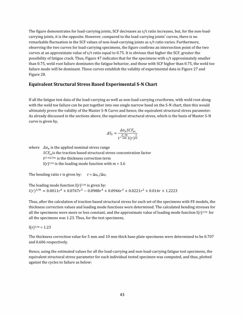
43
The figure demonstrates for load-carrying joints, SCF decreases as s/t ratio increases, but, for the non-load-
carrying joints, it is the opposite. However, compared to the load-carrying joints’ curves, there is no
remarkable fluctuation in the SCF values of non-load-carrying joints as s/t ratio varies. Furthermore,
observing the two curves for load-carrying specimens, the figure confirms an intersection point of the two
curves at an approximate value of s/t ratio equal to 0.75. It is obvious that higher the SCF, greater the
possibility of fatigue crack. Thus, Figure 47 indicates that for the specimens with s/t approximately smaller
than 0.75, weld root failure dominates the fatigue behavior, and those with SCF higher than 0.75, the weld toe
failure mode will be dominant. These curves establish the validity of experimental data in Figure 27 and
Figure 28.
Equivalent Structural Stress Based Experimental S-N Chart
If all the fatigue test data of the load-carrying as well as non-load-carrying cruciforms, with weld root along
with the weld toe failure can be put together into one single narrow band on the S-N chart, then this would
ultimately prove the validity of the Master S-N Curve and hence, the equivalent structural stress parameter.
As already discussed in the sections above, the equivalent structural stress, which is the basis of Master S-N
curve is given by,
( )
where is the applied nominal stress range
is the traction based structural stress concentration factor
t(2-m)/2m is the thickness correction term
I(r)1/m is the loading mode function with m = 3.6
The bending ratio r is given by: r = ∆sb /∆sS
The loading mode function I(r)1/m is given by:
( )
Thus, after the calculation of traction based structural stress for each set of the specimens with FE models, the
thickness correction values and loading mode functions were determined. The calculated bending stresses for
all the specimens were more or less constant, and the approximate value of loading mode function I(r)1/m for
all the specimens was 1.23. Thus, for the test specimens,
I(r)1/m = 1.23
The thickness correction value for 5 mm and 10 mm thick base plate specimens were determined to be 0.707
and 0.606 respectively.
Hence, using the estimated values for all the load-carrying and non-load-carrying fatigue test specimens, the
equivalent structural stress parameter for each individual tested specimen was computed, and thus, plotted
against the cycles to failure as below:
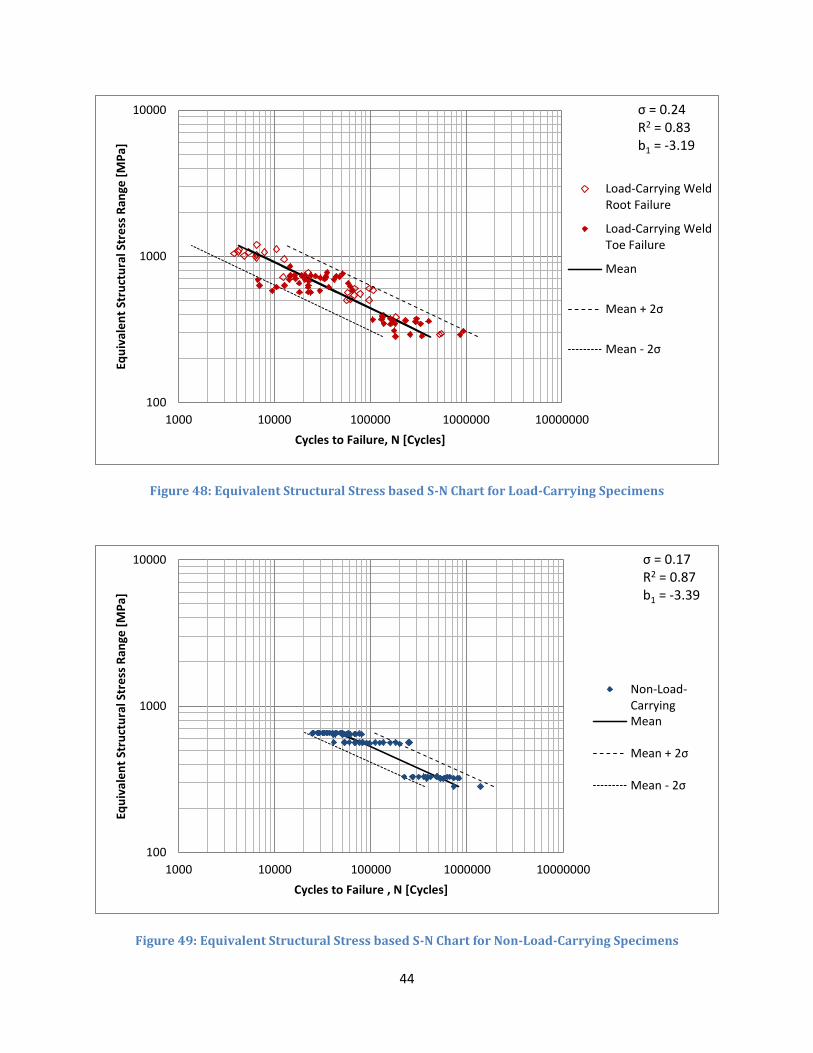
44
Figure 48: Equivalent Structural Stress based S-N Chart for Load-Carrying Specimens
Figure 49: Equivalent Structural Stress based S-N Chart for Non-Load-Carrying Specimens
100
1000
10000
1000 10000 100000 1000000 10000000
Equ
ival
en
t St
ruct
ura
l Str
ess
Ran
ge [
MP
a]
Cycles to Failure, N [Cycles]
Load-Carrying WeldRoot Failure
Load-Carrying WeldToe Failure
Mean
Mean + 2σ
Mean - 2σ
σ = 0.24 R2 = 0.83 b1 = -3.19
100
1000
10000
1000 10000 100000 1000000 10000000
Equ
ival
en
t St
ruct
ura
l Str
ess
Ran
ge [
MP
a]
Cycles to Failure , N [Cycles]
Non-Load-CarryingMean
Mean + 2σ
Mean - 2σ
σ = 0.17 R2 = 0.87 b1 = -3.39
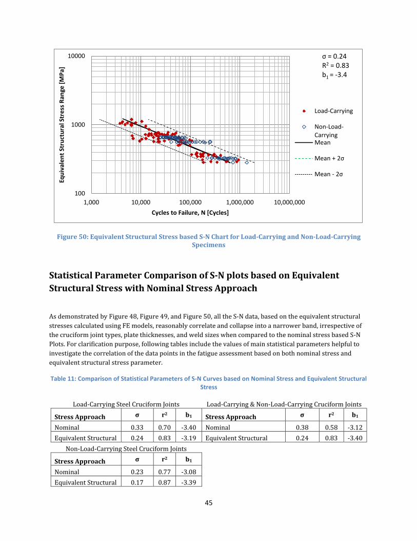
45
Figure 50: Equivalent Structural Stress based S-N Chart for Load-Carrying and Non-Load-Carrying Specimens
Statistical Parameter Comparison of S-N plots based on Equivalent
Structural Stress with Nominal Stress Approach
As demonstrated by Figure 48, Figure 49, and Figure 50, all the S-N data, based on the equivalent structural
stresses calculated using FE models, reasonably correlate and collapse into a narrower band, irrespective of
the cruciform joint types, plate thicknesses, and weld sizes when compared to the nominal stress based S-N
Plots. For clarification purpose, following tables include the values of main statistical parameters helpful to
investigate the correlation of the data points in the fatigue assessment based on both nominal stress and
equivalent structural stress parameter.
Table 11: Comparison of Statistical Parameters of S-N Curves based on Nominal Stress and Equivalent Structural Stress
Load-Carrying Steel Cruciform Joints Load-Carrying & Non-Load-Carrying Cruciform Joints
Stress Approach σ r2 b1 Stress Approach σ r2 b1
Nominal 0.33 0.70 -3.40 Nominal 0.38 0.58 -3.12
Equivalent Structural 0.24 0.83 -3.19 Equivalent Structural 0.24 0.83 -3.40
Non-Load-Carrying Steel Cruciform Joints
Stress Approach σ r2 b1
Nominal 0.23 0.77 -3.08 Equivalent Structural 0.17 0.87 -3.39
100
1000
10000
1,000 10,000 100,000 1,000,000 10,000,000
Equ
ival
en
t St
ruct
ura
l Str
ess
Ran
ge [
MP
a]
Cycles to Failure, N [Cycles]
Load-Carrying
Non-Load-CarryingMean
Mean + 2σ
Mean - 2σ
σ = 0.24 R2 = 0.83 b1 = -3.4
46
In Table 11, the standard deviation values of load-carrying, non-load-carrying, and both load and non-load
carrying joints specimen data together, were 0.33, 0.23, and 0.38 respectively when the nominal stresses
were plotted in the S-N chart. However, significant reduction of the values followed when instead of
equivalent structural stresses replaced the nominal stresses. The standard deviation values dropped from
0.33 to 0.24 for load-carrying joints data, 0.23 to 0.17 for non-load-carrying joints data, and 0.38 to 0.24 for
both load and non-load-carrying joints data put together. The substantial reduction in standard deviation
indicates the strong correlation of the data points and possibility of a single master S-N curve. Similarly, the r-
squared values increased with the use of equivalent structural stress parameter over the nominal stress. The
closer the value of R2 to 1, the better the regression line fits the data set. From the numerical values of R2 in
the provided table, the equivalent structural approach has higher values, ranging from 0.83 to 0.87, and
hence, gives better curve fit.
Comparing all the standard deviation and R2 values in the table above, it can be concluded that there existed
the least correlation when the load-carrying and non-load-carrying specimens fatigue data were put together
in an S-N plot based on nominal stress approach. However, with the use of equivalent structural stress, the
standard deviation is reasonably lowered and the correlation is remarkably improved.
Conclusion
Not only can the traction based structural stress parameter be calculated consistently with the provided traction
stress approach, but it also serves an effective fatigue parameter in order to correlate the fatigue behavior of
welded joints irrespective of the joint types, plate thicknesses, the weld sizes along with the loading modes. When
associated with the fracture mechanics concept, a master S-N curve can be generated with the basis of equivalent
structural stress parameter. This parameter captures the geometric stress concentration factor, the loading mode,
and the plate thickness effects in different kind of joints, and consequently, provides a significant improvement in
the correlation of fatigue data. Thus, the master S-N curve approach, along with the application of equivalent
structural stress concept, serves as a good platform for effective fatigue assessment of welded joints in the ships
and offshore structures.
47
V. Conclusions
In this study, a brief literature review of the ABS Publication 115, Guide for The Fatigue Assessment of
Offshore Structures, was performed. Further, the fatigue tests were performed on the load-carrying and non-
load-carrying cruciform weld details, typical in marine structures. The experimental results were
subsequently evaluated, and compared with the ABS fatigue assessment methods. Finally, the master S-N
Curve approach was utilized, and the experimental data were evaluated using the equivalent structural stress
parameter. The findings of this study can be summarized as follows.
i. Nominal stress definition is consistent; however, the determination of nominal stresses in the
complex structures is a challenge in itself. There is virtually no correlation in the S-N data based on
nominal stress approach.
ii. Hot-Spot stress approach reduces the number of eight S-N curves to a single class “E” S-N curve.
However, hot-spot stress, when determined using FE model, is sensitive to the element type and the
mesh size, thus, it is not consistent. In addition, in its calculation procedure, no clear justification to
the reference locations, 0.5t and 1.5t, is provided. This approach is not applicable to the FE models of
simple connections like cruciform joints.
iii. Experimental results indicate that the fatigue lives of the structures vary with the variation in the
thicknesses of the base plates, even if the thickness is lower than the reference thickness provided in
ABS guidelines.
iv. The load-carrying steel cruciform joints have two fatigue failure modes: weld root failure and weld
toe failure, whereas, the non-load-carrying steel cruciform joints have only weld toe failures. The
stress concentration curves developed from the finite element models of the cruciform joints display
a critical point for the load-carrying joints where the failure mode transitions from weld root to weld
toe, and that point is in the vicinity of s/t ratio = 0.75.
v. The equivalent structural stress is consistent with the master S-N curve, and it correlates the fatigue
experimental data reasonably well. It takes into account the influence of thickness as well as loading
mode variations, and considers the stress concentration factor of different geometry. Thus, this
parameter makes it possible to plot the fatigue data of several joint types of varying thicknesses and
loading modes into a single S-N chart, with relatively narrow scatter band. Overall, in fatigue
evaluation methods, the equivalent structural stress serves as a very good fatigue parameter.
48
References
“Commentary on the Guide for the Fatigue Assessment of Offshore Structures,” ABS, April, 2003.
“Fatigue Design of Offshore Steel Structures,” DNV RP-C203, April 2010.
“Guide for the Fatigue Assessment of Offshore Structures,” ABS, April, 2003.
Doerk, O., Fricke, W., and Weissenborn, C., “Comparison of Different Calculation Methods for Structural Stresses at Welded Joints,” International Journal of Fatigue, Vol. 25, pp.359-369, 2003.
Dong, P., Hong, J.K., Osage, D.A., Dewees, D.J., and Prager, M., “Master S-N Curve Method An Implementation for Fatigue Evaluation of Welded Components in the ASME B&PV Code, Section VIII, Division 2, and API 579-1/ASME FFS-1, Welding Research Council Bulletin, No. 523, 2010, New York, New York.
Dong, P., “Verity Weld Fatigue Method in Fe-Safe Using ANSYS,” Columbus, Ohio.
Fricke, W., and Kahl, A., “Comparison of Different Structural Stress Approaches for Fatigue Assessment of Welded Ship Structures,” Marine Structures, Vol. 18, pp.473-488, 2005.
Fricke, W., “Fatigue Analysis of Welded Joints: State of Development,” Marine Structures, Vol. 16, pp.185-200, 2003.
Huang, T.D., Harbison, M., Kvidahl, L., Niolet, D., Walks, J., Stefanick, K., Phillipi, M., Dong, p., DeCan, L., Caccese, V., Blomquist, P., Kihl, D., Wong, R., Nappi, N., gardner, J., Wong, C., Bjornson, M., and Manuel, A., “Overwelding and Distortion Control for Naval Surface Combatants,” SNAME Journal of…………………………………….
Iwata, T and Matsuoka, K., “Fatigue Strength of CP Grade 2 Titanium Fillet Welded Joint for Ship Structure,” Welding in the world, Vol. 48, No.7-8, pp.40-47, 2004.
Kihl, D.P. and Sarkani, S., “Thickness Effects on the Fatigue Strength of Welded Steel Cruciforms,” International Journal of Fatigue, Vol. 19, No. 1, pp. S311-S316, 199, Great Britain.
Kim, M.H., Kang, S.W., Kim, J.H. Kim, K.S., Kang, J.K., and Heo, J.H., “An Experimental Study on the Fatigue Strength Assessment of Longi-Web Connections in Ship Structures Using Structural Stress,” International Journal of Fatigue, Vol. 32, pp.318-329, 2010.
Maddox, S.J., “Recommended Hot-Spot Stress Design S-N Curves for Fatigue Assessment of FPSOs,” Proceedings of International Journal of Offshore and Polar Engineering, June 17-22, 2001, Stavanger, Norway.
Maddox, S.J., “Fatigue Design Rules for Welded Structures,” Progress in Structural Engineering and Materials, Vol. 2, No. 1, pp. 102-109, Jan-Mar, 2000.
Maddox, S.J., “Review of Fatigue Assessment Procedures for Welded Aluminum Structures,” International Journal of Fatigue, Paper JIJF1005, Vol. 25, No. 12, pp. 1359-1378, December, 2003.
Schijve, J., “Fatigue of Structures and Materials in the 20th Century and the State of the Art,” International Journal of Fatigue, Vol. 25, pp.679-702, 2003.
Wang, X. and Cheng, Z., “Sensitivity of Fatigue Assessment to the Use of Different Reference S-N Curves,” Proceedings of 22nd International Conference on Offshore Mechanics and Arctic Engineering, June 8-13, 2003, Cancun, Mexico.

49
Appendices
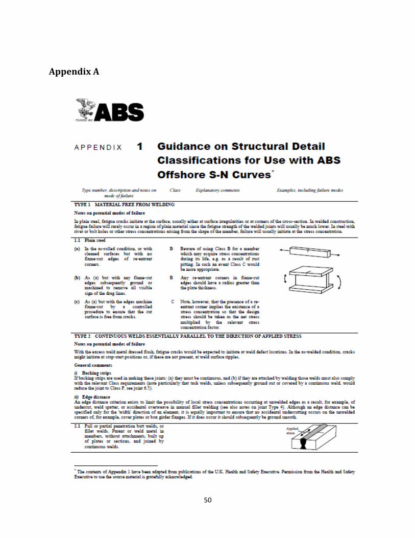
50
Appendix A
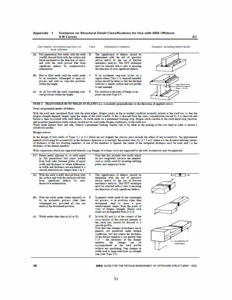
51
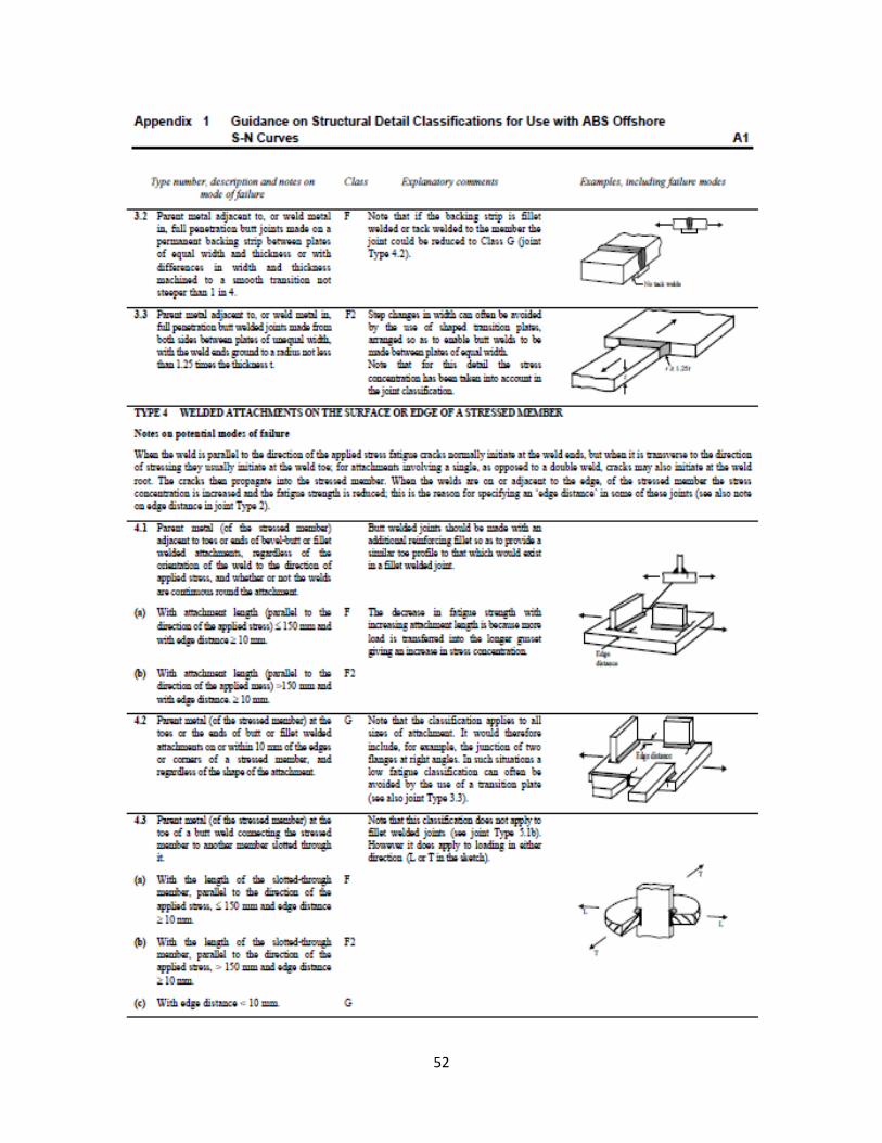
52
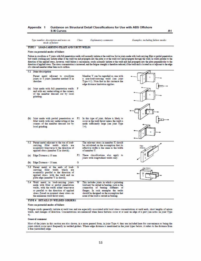
53
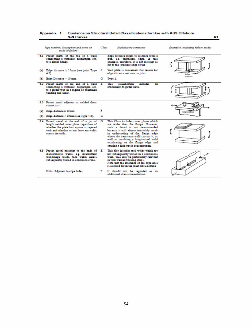
54

55
Appendix B
Stiffness Calculation
The stiffness of the specimen is performed using the recorded data of force and displacement. The stiffness
curve is determined according to the definition as the load divided by the displacement.
[kips/in]
The initial stiffness of the welded cruciform is considered to be an average stiffness of first 1000 cycles, to be
consistent. Then, the cycle count where the initial average stiffness of 1000 cycles is reduced by 50% is the
fatigue life of the specimen.
56
Vita The author was born in Kathmandu, Nepal. She received her Bachelor’s degree in Naval Architecture and
Marine Engineering from the University of New Orleans in 2011. She continued with the graduate study
under the same concentration after her graduation. She will obtain her Master’s degree in Naval Architecture
& Marine Engineering in May 2013. She has worked for Dr. Pingsha Dong as a graduate research assistant in
the School of Naval Architecture & Marine Engineering for two years. She interned previously at American
Bureau of Shipping, Houston, TX.