Faster Fully Homomorphic Encryption:Bootstrapping in less than 0.1 Seconds

Ilaria Chillotti1, Nicolas Gama2,1, Mariya Georgieva3, and Malika Izabachene4

1 Laboratoire de Mathematiques de Versailles, UVSQ, CNRS, UniversiteParis-Saclay, 78035 Versailles, France

2 Inpher, Lausanne, Switzerland3 Gemalto, 6 rue de la Verrerie 92190, Meudon, France

4 CEA LIST, Point Courrier 172, 91191 Gif-sur-Yvette Cedex, France

Abstract. In this paper, we revisit fully homomorphic encryption(FHE) based on GSW and its ring variants. We notice that the internalproduct of GSW can be replaced by a simpler external product betweena GSW and an LWE ciphertext.We show that the bootstrapping scheme FHEW of Ducas and Miccian-cio [14] can be expressed only in terms of this external product. As aresult, we obtain a speed up from less than 1 second to less than 0.1seconds. We also reduce the 1GB bootstrapping key size to 24MB, pre-serving the same security levels, and we improve the noise propagationoverhead by replacing exact decomposition algorithms with approximateones.Moreover, our external product allows to explain the unique asymmetryin the noise propagation of GSW samples and makes it possible to eval-uate deterministic automata homomorphically as in [16] in an efficientway with a noise overhead only linear in the length of the tested word.Finally, we provide an alternative practical analysis of LWE basedscheme, which directly relates the security parameter to the error rateof LWE and the entropy of the LWE secret key.Keywords: Fully Homomorphic Encryption, Bootstrapping, Lattices,LWE, GSW

1 Introduction

Fully homomorphic encryption (FHE) allows to perform computations over en-crypted data without decrypting them. This concept has long been regardedas an open problem until the breakthrough paper of Gentry in 2009 [18] whichdemonstrates the feasibility of computing any function on encrypted data. Sincethen, many constructions have appeared involving new mathematical and algo-rithmic concepts and improving efficiency.

In homomorphic encryption, messages are encrypted with a noise that growsat each homomorphic evaluation of an elementary operation. In a somewhat en-cryption scheme, the number of homomorphic operations is limited, but can bemade asymptotically large using bootstrapping [18]. This technical trick intro-duced by Gentry allows to evaluate arbitrary circuits by essentially evaluating

the decryption function on encrypted secret keys. This step has remained verycostly until the recent paper of Ducas and Micciancio [14], which presented avery fast bootstrapping procedure running in around 0.69 second, making an im-portant step towards practical FHE for arbitrary NAND circuits. In this paper,we further improve the bootstrapping procedure.

We first provide an intuitive formalization of LWE/RingLWE on numbers orpolynomials over the real torus, obtained by combining the Scale-Invariant-LWEproblem of [12] or the LWE normal form of [13] with the General-LWE problem ofBrakerski-Gentry-Vaikutanathan [6]. We call TLWE this unified representationof LWE ciphertexts, which encode polynomials over the Torus. Its security relieseither on the hardness of general or ideal lattice reduction, depending on thechoice of dimensions. Using the same formalism, we extend the GSW/RingGSWciphertexts to TGSW, which is the combined analogue of Gentry-Sahai-Water’sciphertexts from [19, 3], and which can also instantiate the ring version used inDucas-Micciancio scheme [14] in the FHEW cryptosystem. Similarly, a TGSWciphertext encodes an integer polynomial message, and depending on the choiceof dimesions, its security is also based on (worst-case) generic or ideal latticereduction algorithms. TLWE and TGSW are basically dual to each other, andthe main idea of our efficiency result comes from the fact that these two schemescan directly be combined together to map the external product of their twomessages into a TLWE sample. A similar operation has been independentlyused in [8] to speed-up GSW computation.

Since a TGSW sample is essentially a matrix whose individual rows areTLWE samples, the external product TGSW times TLWE is much quicker thanthe usual internal product TGSW times TGSW used in previous work. Thiscould mostly be understood as comparing the speed of the computation of amatrix-vector product to a matrix-matrix product. As a result, we obtain asignificant improvement (12 times faster) of the most efficient bootstrappingprocedure [14]; it now runs in less than 0.052s. Different improvements of the[14] procedure have been proposed in [4]: a first one where the authors showhow to bootstrap several bits at the same time, and speed up the evaluationof a bootstrapped full adder over several bits, and a second one to parallelizethe bootstrapping. Their first improvement can still be applied on top of ourconstruction, however, the second one is superseeded by our external product.

We also analyze the case of leveled encryption. Using an external productmeans that we lose some composability properties in the design of homomorphiccircuits. This corresponds to circuits where boolean gates have different kinds ofwires that cannot be freely interconnected. Still, we show that we maintain theexpressiveness of the whole binary decision diagram and automata-based logic,which was introduced in [16] with the GSW-GSW internal product, and wetighten the analysis. Indeed, while it was impractical (10 transitions per secondin the ring case, and impractical in the non-ring case), we show that the TGSW-TLWE external product enables to evaluate up to 5000 transitions per second, ina leveled homomorphic manner. We also refine the mapping between automataand homomorphic gates, and reduce the number of homomorphic operations to

2

test a word with a deterministic automata. This allows to compile and evaluateconstant-time algorithms (i.e. with data-independent control flow) in a leveledhomomorphic manner, with only sub-linear noise overhead in the running time.

We also propose a new security analysis where the security parameter isdirectly expressed as a function of the entropy of the secret and the error rate.For the parameters that we propose in our implementation, we predict 188-bitsof security for both the bootstrapping key and the keyswitching key.

Roadmap. In Section 2, we give mathematical definitions and a quick overviewof the classical version of LWE-based schemes. In Section 3, we generalize LWEand GSW schemes using a torus representation of the samples. We also reviewthe arithmetic operations over the torus and introduce our main theorem char-acterizing the new morphism between TLWE and TGSW. As a proof of concept,we present two main applications in Section 4 where we explain our fast boot-strapping procedure, and in Section 5, we present efficient leveled evaluation ofdeterministic automata, and apply it on a constant-time algorithm with loga-rithmic memory. Finally, we provide a practical security analysis in Section 6.

2 Background

Notation. In the rest of the paper we will use the following notations. Thesecurity parameter will be denoted as λ. The set 0, 1 (without any structure)will be written B. The real Torus R/Z, called T set of real numbers modulo 1. Rdenotes the ring of polynomials Z[X]/(XN + 1). TN [X] denotes R[X]/(XN + 1)mod 1. Finally, we note by Mp,q(E) the set of matrices p× q with entries in E.

This section combines some algebra theory, namely abelian groups, commu-tative rings, R-modules, and on some metrics of the continuous field R.

Definition 2.1 (R-module). Let (R,+,×) be a commutative ring. We say thata set M is a R-module when (M,+) is an abelian group, and when there exists anexternal operation · which is bi-distributive and homogeneous. Namely, ∀r, s ∈ Rand x, y ∈M , 1R · x = x, (r + s) · x = r · x+ s · x, r · (x+ y) = r · x+ r · y, and(r × s) · x = r · (s · x).

Any abelian group is by construction a Z-module for the iteration (or ex-ponentiation) of its own law. In this paper, one of the most important abeliangroup we use is the real torus T, composed of all reals modulo 1 (R mod 1).The torus is not a ring, since the real internal product is not compatible withthe modulo 1 projection (expressions like 0× 1

2 are undefined). But as an addi-tive group, it is a Z-module, and the external product · from Z×T to T, like in0 · 12 = 0, is well defined. More importantly, we recall that for all positive integersN and k, (TN [X]k,+, •) is a R-module.

A R-module M shares many arithmetic operations and constructions withvector spaces: vectors Mn or matrices Mn,m(M) are also R-modules, and theirleft dot product with a vector in Rn or left matrix product inMk,n(R) are bothwell defined.

3

Gaussian Distributions Let σ ∈ R+ be a parameter and k ≥ 1 the dimension.For all x, c ∈ Rk, we note ρ

σ,c(x) = exp(−π ‖x− c‖2 /σ2). If c is omitted,then it is implicitly 0. Let S be a subset of Rk, ρσ,c(S) denotes

∑x∈S

ρσ,c(x)

or∫x∈S

ρσ,c(x).dx. For all closed (continuous or discrete) additive subgroup

M ⊆ Rk, then ρσ,c(M) is finite, and defines a (restricted) Gaussian Distribution

of parameter σ, standard deviation√

2/πσ and center c over M , with the densityfunction DM,σ,c(x) = ρ

σ,c(x)/ρσ,c(M). Let L be a discrete subgroup of M , thenthe Modular Gaussian distribution over M/L exists and is defined by the densityDM/L,σ,c(x) = DM,σ,c(x + L). Furthermore, when span(M) = span(L), thenM/L admits a uniform distribution of constant density UM/L. In this case, thesmoothing parameter η

M,ε(L) of L in M is defined as the smallest σ ∈ R suchthat supx∈M |DM/L,σ,c(x) − UM/L| ≤ ε · UM/L. If M is omitted, it implicitely

means Rk.

Subgaussian Distributions A distribution X over R is σ-subgaussian iff itsatisfies the Laplace-transformation bound: ∀t ∈ R,E(exp(tX)) ≤ exp(σ2t2/2).By Markov’s inequality, this implies that the tails of X are bounded by the Gaus-sian function of standard deviation σ: ∀x > 0,P(|X| ≥ x) ≤ 2 exp(−x2/2σ2). Asan example, the Gaussian distribution of standard deviation σ (i.e. parameter√π/2σ), the equi-distribution on −σ, σ, and the uniform distribution over

[−√

3σ,√

3σ], which all have standard deviation σ, are σ-subgaussian5. If X andX ′ are two independent σ and σ′-subgaussian variables, then for all α, β ∈ R,αX + βX ′ is

√α2σ2 + β2σ′2-subgaussian.

Distance and Norms We use the standard ‖·‖p and ‖·‖∞ norms for scalars andvectors over the real field or over the integers. By extension, the norm ‖P (X)‖pof a real or integer polynomial P ∈ R[X] is the norm of its coefficient vector. Ifthe polynomial is modulo XN + 1, we take the norm of its unique representativeof degree ≤ N − 1.

By abuse of notation, we write ‖x‖p = minu∈x+Zk(‖u‖p) for all x ∈ Tk. It is

the p-norm of the representative of x with all coefficients in ]− 12 ,

12 ]. Although

it satisfies the separation and the triangular inequalities, this notation is nota norm, because it lacks homogeneity6, and Tk is not a vector space either.But we have ∀m ∈ Z, ‖m · x‖p ≤ |m| ‖x‖p. By extension, we define ‖a‖p for apolynomial a ∈ TN [X] as the p- norm of its unique representative in R[X] ofdegree ≤ N − 1 and with coefficients in ]− 1

2 ,12 ].

5 For the first two distributions, it is tight, but the uniform distribution over[−√

3σ,√

3σ] is even 0.78σ-subgaussian6 Mathematically speaking, a more accurate notion would be distp(x,y) = ‖x− y‖p,

which is a distance. However, the norm symbol is clearer for almost all practicalpurposes.

4

Definition 2.2 (Infinity norm over Mp,q(TN [X])). Let A ∈ Mp,q(TN [X]).We define the infinity norm of A as

‖A‖∞ = maxi∈[[1,p]]j∈[[1,q]]

‖ai,j‖∞ .

Concentrated distribution on the Torus, Expectation and VarianceA distribution X on the torus is concentrated iff. its support is included in aball of radius 1

4 of T, except for negligible probability. In this case, we definethe variance Var(X ) and the expectation E(X ) of X as respectively Var(X ) =minx∈T

∑p(x)|x − x|2 and E(X ) as the position x ∈ T which minimizes this

expression. By extension, we say that a distribution X ′ over Tn or TN [X]k isconcentrated iff. each coefficient has an independent concentrated distributionon the torus. Then the expectation E(X ′) is the vector of expectations of eachcoefficient, and Var(X ′) denotes the maximum of each coefficient’s Variance.

These expectation and variance over T follow the same linearity rules thantheir classical equivalent over the reals.

Fact 2.3. Let X1,X2 be two independent concentrated distributions on eitherT,Tn or TN [X]k, and e1, e2 ∈ Z such that X = e1 · X1 + e2 · X2 remains concen-trated, then E(X ) = e1 ·E(X1)+e2 ·E(X2) and Var(X ) ≤ e2

1 ·Var(X1)+e22 ·Var(X2).

Also, subgaussian distributions with small enough parameters are necessarilyconcentrated:

Fact 2.4. Every distribution X on either T,Tn or TN [X]k where each coefficientis σ-subgaussian where σ ≤ 1/

√32 log(2)(λ+ 1) is a concentrated distribution:

a fraction 1− 2−λ of its mass is in the interval [− 14 ,

14 ].

2.1 Learning With Error problem

The Learning With Errors (LWE) problem was introduced by Regev in 2005 [25].The Ring variant, called RingLWE, was introduced by Lyubashevsky, Peikertand Regev in 2010 [23]. Both variants are nowadays extensively used for theconstruction of lattice-based Homomorphic Encryption schemes. In the originaldefinition [25], a LWE sample has its right member on the torus and is definedusing continuous Gaussian distributions. Here, we will work entirely on the realtorus, employing the same formalism as the Scale Invariant LWE (SILWE) schemein [12], or LWE scale-invariant normal form in [13]. Without loss of generality,we refer to it as LWE.

Definition 2.5 ((Homogeneous) LWE). Let n ≥ 1 be an integer, α ∈ R+ bea noise parameter and s be a uniformly distributed secret in some bounded setS ⊂ Zn. Denote by DLWE

s,α the distribution over Tn × T obtained by sampling acouple (a, b), where the left member a ∈ Tn is chosen uniformly random and theright member b = a · s+ e. The error e is a sample from a gaussian distributionwith parameter α.

5

– Search problem: given access to polynomially many LWE samples, find s ∈ S.– Decision problem: distinguish between LWE samples and uniformly random

samples from Tn × T.

Both the LWE search or decision problems are reducible to each other, andtheir average case is asymptotically as hard as worst-case lattice problems. Inpractice, both problems are also intractable, and their hardness increases withthe the entropy of the key set S (i.e. n if keys are binary) and α ∈]0, ηε(Z)[.

Regev’s encryption scheme [25] is the following: Given a discrete messagespace M ⊂ T, for instance 0, 1

2, a message µ ∈ M is encrypted by summingup the trivial LWE sample (0, µ) of µ to a Homogeneous LWE sample (a, b) ∈Tn+1 with respect to a secret key s ∈ Bn and a noise parameter α ∈ R+. Thesemantic security of the scheme is equivalent to the LWE decisional problem. Thedecryption of a sample c = (a, b) consists in computing this quantity ϕs(a, b) =b− s · a, which we call the phase of c, and to round it to the nearest element inM. Decryption is correct with overwhelming probability 1− 2−p provided thatthe parameter α is O(R/

√p) where R is the packing radius of M.

3 Generalization

In this section we extend this presentation to rings, following the generalizationof [6], and also to GSW [19].

3.1 TLWE

We first define TLWE samples, together with the search and decision problems.In the following, ciphertexts are viewed as normal samples.

Definition 3.1 (TLWE samples). Let k ≥ 1 be an integer, N a power of 2,and α ≥ 0 be a noise parameter. A TLWE secret key s ∈ BN [X]k is a vector of kpolynomials ∈ R = Z[X]/XN +1 with binary coefficients. For security purposes,we assume that private keys are uniformly chosen, and that they actually containn ≈ Nk bits of entropy. The message space of TLWE samples is TN [X]. A freshTLWE sample of a message µ ∈ TN [X] with noise parameter α under the keys is an element (a, b) ∈ TN [X]k × TN [X], b ∈ TN [X] has Gaussian distributionDTN [X],α,s•a+µ around µ+s ·a. The sample is random iff its left member a (also

called mask) is uniformly random ∈ TN [X]k (or a sufficiently dense submodule7 ), trivial if a is fixed to 0, noiseless if α = 0, and homogeneous iff its messageµ is 0.

7 A submodule G is sufficiently dense if there exists an intermediate submodule Hsuch that G ⊆ H ⊆ Tn, the relative smoothing parameter ηH,ε(G) is ≤ α, andH is the orthogonal in Tn of at most n − 1 vectors of Zn. This definition allowsto convert any (Ring)-LWE with non-binary secret to a TLWE instance via binarydecomposition.

6

– Search problem: given access to polynomially many fresh random homoge-neous TLWE samples, find their key s ∈ BN [X]k.

– Decision problem: distinguish between fresh random homogeneous TLWEsamples from uniformly random samples from TN [X]k+1.

This definition is the analogue on the torus of the Gereral-LWE problem of [6].It allows to consider both LWE and RingLWE as a single problem. ChoosingN large and k = 1 corresponds to the classical (bin)RingLWE (over cyclotomicrings, and up to a scaling factor q). When N = 1 and k large, then R andTN [X] respectively collapses to Z and T, and TLWE is simply bin-LWE (up tothe same scaling factor q). Other choices of N, k give some continuum betweenthe two extremes, with a security that varies between worst-case ideal latticesto worst-case regular lattices.

Thanks to the underlying R-module structure, we can sum TLWE samples,or we can make integer linear or polynomial combinations of samples with coef-ficients in R. However, each of these combinations increases the noise inside thesamples. They are therefore limited to small coefficients.

We additionally define a function called the phase of a TLWE sample, thatwill be used many times. The phase computation is the first step of the classicaldecryption algorithm, and uses the secret key.

Definition 3.2 (Phase). Let c = (a, b) ∈ TN [X]k × TN [X] and s ∈ BN [X]k,we define the phase of the sample as ϕs(c) = b− s • a.The phase is linear over TN [X]k+1 and is (kN + 1)-lipschitzian for the `∞ dis-tance: ∀x,y ∈ TN [X]k+1, ‖ϕs(x)− ϕs(y)‖∞ ≤ (kN + 1) ‖x− y‖∞.

Note that a TLWE sample contains noise, that its semantic is only function ofits phase, and that the phase has the nice property to be lipschitzian. Together,these properties have many interesting implications. In particular, we can alwayswork with approximations, since two samples at a short distance on TN [X]k+1

share the same properties: they encode the same message, and they can in generalbe swapped. This fact explains why we can work and describe our algorithms onthe infinite Torus.

Given a finite message space M ⊆ TN [X], the (classical) decryption algo-rithm computes the phase ϕs(c) of the sample, and returns the closest µ ∈ M.It is easy to see that if c is a fresh TLWE sample of µ ∈M with gaussian noiseparameter α, the decryption of c over M is equal to µ as soon as α is Θ(

√λ)

times smaller than the packing radius of M. However decryption is harder todefine for non-fresh samples. In this case, correctness of the decryption proce-dure involves a recurrence formula between the decryption of the sum and thesum of the decryption of the inputs conditioned by the noise parameters. In ad-dition, message spaces of the input samples can be in different subgroups of T.To raise the limitations of the decryption function, we will instead use a math-ematical definition of message and error by reasoning directly on the followingΩ-probability space.

7

Definition 3.3 (The Ω-probability space). Since samples are either inde-pendent (random, noiseless, or trivial) fresh c← TLWEs,α(µ), or linear combi-nation c =

∑pi=1 ei ·ci of other samples, the probability space Ω is the product of

the probability spaces of each individual fresh samples c with the TLWE distribu-tions defined in definitions 3.1, and of the probability spaces of all the coefficients(e1, . . . , ep) ∈ Rp or Zp that are obtained with randomized algorithm.

In other words, instead of viewing a TLWE sample as a fixed value which isthe result of one particular event in Ω, we will consider all the possible valuesat once, and make statistics on them.

We now define functions on TLWE samples: message, error, noise variance,and noise norm. These functions are well defined mathematically, and can beused in the analysis of various algorithms. However, they cannot be directlycomputed or approximated in practice.

Definition 3.4. Let c be a random variable ∈ TN [X]k+1, which we’ll interpretas a TLWE sample. All probabilities are on the Ω-space. We say that c is avalid TLWE sample iff there exists a key s ∈ BN [X]k such that the distributionof the phase ϕs(c) is concentrated. If c is trivial, all keys s are equivalent, elsethe mask of c is uniformly random, so s is unique. We then define:

– the message of c, denoted as msg(c) ∈ TN [X] is the expectation of ϕs(c);

– the error, denoted Err(c), is equal to ϕs(c)−msg(c);

– Var(Err(c)) denotes the variance of Err(c), which is by definition also equalto the variance of ϕs(c);

– finally, ‖Err(c)‖∞ denotes the maximum amplitude of Err(c) (possibly withoverwhelming probability).

Unlike the classical decryption algorithm, the message function can be viewedas an ideal black box decryption function, which works with infinite precisioneven if the message space is continuous. Provided that the noise amplitude re-mains smaller than 1

4 , the message function is perfectly linear. Using these intu-itive and intrinsic functions will considerably ease the analysis of all algorithmsin this paper. In particular, we have:

Fact 3.5. Given p valid and independent TLWE samples c1, . . . , cp under thesame key s, and p integer polynomials e1, . . . , ep ∈ R, if the linear combinationc =

∑pi=1 ei • ci is a valid TLWE sample, it satisfies: msg(c) =

∑pi=1 ei •msg(ci),

with variance Var(Err(c)) ≤ ∑pi=1 ‖ei‖22 · Var(Err(ci)) and noise amplitude

‖Err(c)‖∞ ≤∑pi=1 ‖ei‖1 · ‖Err(ci)‖∞. If the last bound is < 1

4 , then c is neces-sarily a valid TLWE sample (under the same key s).

In order to characterize the average case behaviour of our homomorphicoperations, we shall rely on the heuristic assumption of independence below.This heuristic will only be used for practical average-case bounds. Our worst-case theorems and lemma based on the infinite norm do not use it at all.

8

Assumption 3.6 (Independence Heuristic). All the coefficients of the errorof TLWE or TGSW samples that occur in all the linear combinations we considerare independent and concentrated. More precisely, they are σ-subgaussian whereσ is the square-root of their variance.

This assumption allows us to bound the variance of the noise instead ofits norm, and to provide realistic average-case bounds which often correspondto the square root of the worst-case ones. The error can easily be proved sub-gaussian, since each coefficients are always obtained by convolving Gaussiansor zero-centered bounded uniform distributions. But the independence assump-tion between all the coefficients remains heuristic. Dependencies between coef-ficients may affect the variance of their combinations in both directions. Theindependence of coefficients can be obtained by adding enough entropy in allour decomposition algorithms and by increasing some parameters accordingly,but as noticed in [14], this work-around seems more as a proof artefact, andis experimentally not needed. Since average case corollaries should reflect prac-tical results, we leave the independence of subgaussian samples as a heuristicassumption.

3.2 TGSW

In this section we present a generalized scale invariant version of the FHE schemeGSW [19], that we call TGSW. GSW was proposed Gentry, Sahai and Watersin 2013 [19] and improved in [3], and its security is based on the LWE problem.The scheme relies on a gadget decomposition function, which we also extendto polynomials. But most importantly, the novelty is that our function is anapproximate decomposition, up to some precision parameter. This allows to im-prove running time and memory requirements for a small amount of additionalnoise.

Definition 3.7 (Approximate Gadget Decomposition). Let h ∈Md,k+1(TN [X]) as in (1). We say that Dech,β,ε(v) is a decomposition algorithmon the gadget h with quality β and precision ε if and only if for any TLWE sam-ple v ∈ TN [X]k+1, it efficiently and publicly outputs a small vector u ∈ Rd suchthat ‖u‖∞ ≤ β and ‖u · h− v‖∞ ≤ ε. Furthermore, the expectation of u ·h− vmust to be 0 when v is uniformly distributed in TN [X]k+1

Definition 3.7 is generic, but in the rest of the paper, we will only use thisfixed gadget:

h =

1/Bg . . . 0...

. . ....

1/B`g . . . 0...

. . ....

0 . . . 1/Bg...

. . ....

0 . . . 1/B`g

∈Md,k+1(TN [X]). (1)

9

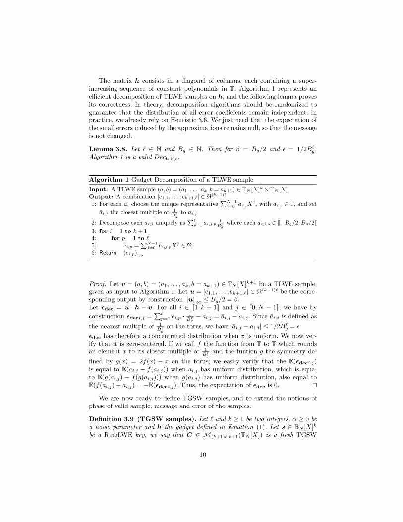
The matrix h consists in a diagonal of columns, each containing a super-increasing sequence of constant polynomials in T. Algorithm 1 represents anefficient decomposition of TLWE samples on h, and the following lemma provesits correctness. In theory, decomposition algorithms should be randomized toguarantee that the distribution of all error coefficients remain independent. Inpractice, we already rely on Heuristic 3.6. We just need that the expectation ofthe small errors induced by the approximations remains null, so that the messageis not changed.

Lemma 3.8. Let ` ∈ N and Bg ∈ N. Then for β = Bg/2 and ε = 1/2B`g,Algorithm 1 is a valid Dech,β,ε.

Algorithm 1 Gadget Decomposition of a TLWE sample

Input: A TLWE sample (a, b) = (a1, . . . , ak, b = ak+1) ∈ TN [X]k × TN [X]Output: A combination [e1,1, . . . , ek+1,`] ∈ R(k+1)`

1: For each ai choose the unique representative∑N−1j=0 ai,jX

j , with ai,j ∈ T, and set

ai,j the closest multiple of 1B`

gto ai,j

2: Decompose each ai,j uniquely as∑`p=1 ai,j,p

1B

pg

where each ai,j,p ∈ [[−Bg/2, Bg/2[[

3: for i = 1 to k + 14: for p = 1 to `5: ei,p =

∑N−1j=0 ai,j,pX

j ∈ R6: Return (ei,p)i,p

Proof. Let v = (a, b) = (a1, . . . , ak, b = ak+1) ∈ TN [X]k+1 be a TLWE sample,given as input to Algorithm 1. Let u = [e1,1, . . . , ek+1,`] ∈ R(k+1)` be the corre-sponding output by construction ‖u‖∞ ≤ Bg/2 = β.Let εdec = u · h − v. For all i ∈ [[1, k + 1]] and j ∈ [[0, N − 1]], we have by

construction εdeci,j =∑`p=1 ei,p •

1Bp

g− ai,j = ai,j − ai,j . Since ai,j is defined as

the nearest multiple of 1B`

gon the torus, we have |ai,j − ai,j | ≤ 1/2B`g = ε.

εdec has therefore a concentrated distribution when v is uniform. We now ver-ify that it is zero-centered. If we call f the function from T to T which roundsan element x to its closest multiple of 1

B`g

and the funtion g the symmetry de-

fined by g(x) = 2f(x) − x on the torus; we easily verify that the E(εdeci,j)is equal to E(ai,j − f(ai,j)) when ai,j has uniform distribution, which is equalto E(g(ai,j) − f(g(ai,j))) when g(ai,j) has uniform distribution, also equal toE(f(ai,j)− ai,j) = −E(εdeci,j). Thus, the expectation of εdec is 0. ut

We are now ready to define TGSW samples, and to extend the notions ofphase of valid sample, message and error of the samples.

Definition 3.9 (TGSW samples). Let ` and k ≥ 1 be two integers, α ≥ 0 bea noise parameter and h the gadget defined in Equation (1). Let s ∈ BN [X]k

be a RingLWE key, we say that C ∈ M(k+1)`,k+1(TN [X]) is a fresh TGSW

10

sample of µ ∈ R/h⊥ with noise parameter α iff C = Z + µ • h whereeach row of Z ∈ M(k+1)`,k+1(TN [X]) is an Homogeneous TLWE sample (of0) with Gaussian noise parameter α. Reciprocally, we say that an elementC ∈ M(k+1)`,k+1(TN [X]) is a valid TGSW sample iff there exists a unique

polynomial µ ∈ R/h⊥ and a unique key s such that each row of C − µ • h is avalid TLWE sample of 0 for the key s. We call the polynomial µ the message ofC, and we denote it by msg(C).

Definition 3.10 (Phase, Error). Let A ∈ M(k+1)`,k+1(TN [X]) be a TGSW

sample for a secret key s ∈ BN [X]k and noise parameter α ≥ 0.We define the phase of A, denoted as ϕs(A) ∈ (TN [X])(k+1)`, as the list of the(k + 1)` TLWE phases of each line of A. In the same way, we define the errorof A, denoted Err(A), as the list of the (k + 1)` TLWE errors of each line of A.

Since TGSW samples are essentially vectors of TLWE samples, they are nat-urally compatible with linear operations. And both phase and message functionsremain linear.

Fact 3.11. Given p valid TGSW samples C1, . . . , Cp of messages µ1, . . . , µp un-der the same key, and with independent error coefficients, and given p integerpolynomials e1, . . . , ep, the linear combination C =

∑pi=1 ei • Ci is a sample of

µ =∑pi=1 ei · µi, with variance Var(C) =

(∑pi=1 ‖ei‖22 · Var(Ci)

)1/2and noise

infinity norm ‖Err(C)‖∞ =∑pi=1 ‖ei‖1 · ‖Err(Ci)‖∞.

Also, the phase remains (1 + kN)-lipschitzian for the infinity norm.

Fact 3.12. For all A ∈Mp,k+1(TN [X]), ‖ϕs(A)‖∞ ≤ (1 + kN) ‖A‖∞.

We finally define the homomorphic product between TGSW and TLWE sam-ples, which corresponding message is simply the product of the two messages ofthe initial samples. A similar product is used in [8]: with our description, we givea new formalization of the product and extend the operation they propose tothe Torus.

Since the left member encodes an integer polynomial, and the right one atorus polynomial, this operator performs a homomorphic evaluation of theirexternal product. Theorem 3.14 (resp. Corollary 3.15) analyzes the worst-case(resp. average-case) noise propagation of this product. Then, corollary 3.16 re-lates this new morphism to the classical internal product between TGSW sam-ples.

Definition 3.13 (External product). We define the product as

: TGSW × TLWE −→ TLWE

(A, b) 7−→ A b = Dech,β,ε(b) ·A.The formula is almost identical to the classical product defined in the original

GSW scheme in [19], except that only one vector needs to be decomposed. Forthis reason, we get almost the same noise propagation formula, with an additionalterm that comes from the approximations in the decomposition.

11

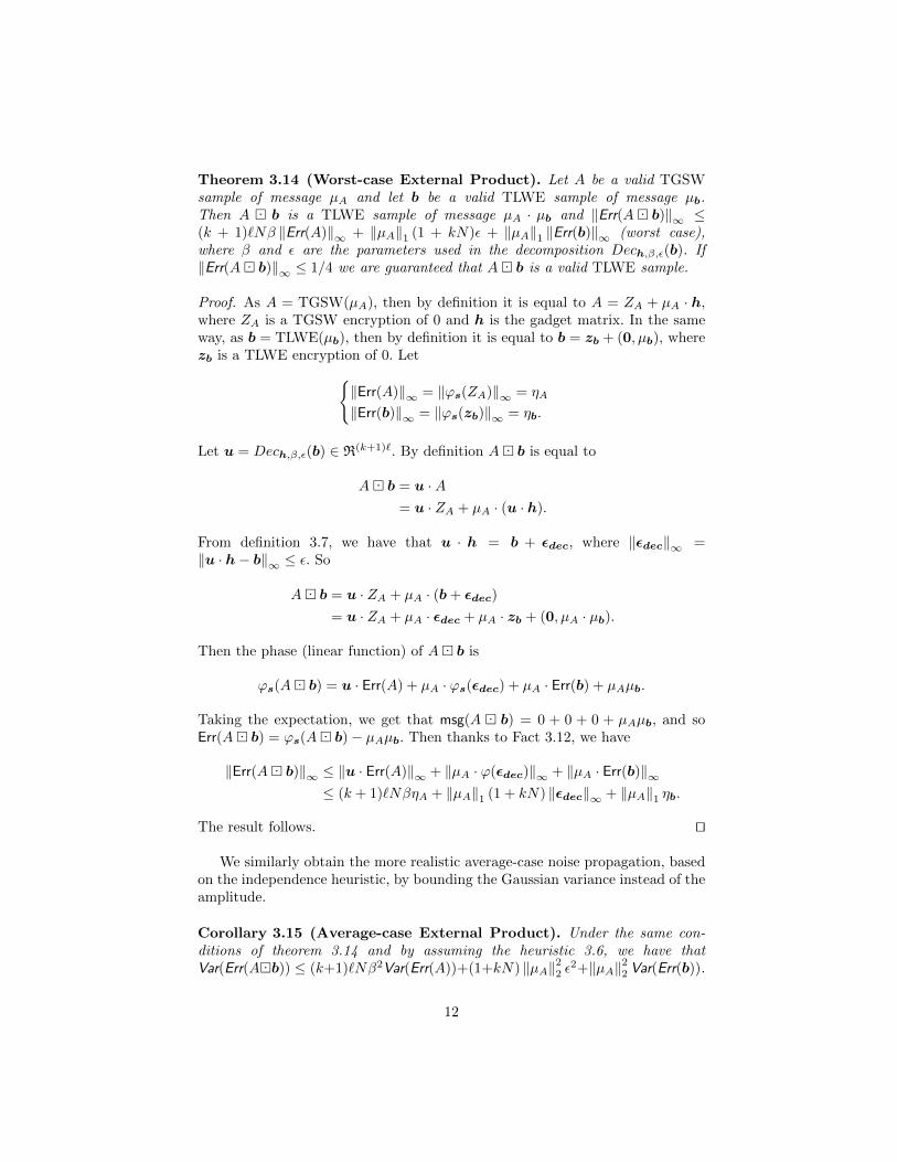
Theorem 3.14 (Worst-case External Product). Let A be a valid TGSWsample of message µA and let b be a valid TLWE sample of message µb.Then A b is a TLWE sample of message µA · µb and ‖Err(A b)‖∞ ≤(k + 1)`Nβ ‖Err(A)‖∞ + ‖µA‖1 (1 + kN)ε + ‖µA‖1 ‖Err(b)‖∞ (worst case),where β and ε are the parameters used in the decomposition Dech,β,ε(b). If‖Err(A b)‖∞ ≤ 1/4 we are guaranteed that A b is a valid TLWE sample.

Proof. As A = TGSW(µA), then by definition it is equal to A = ZA + µA · h,where ZA is a TGSW encryption of 0 and h is the gadget matrix. In the sameway, as b = TLWE(µb), then by definition it is equal to b = zb + (0, µb), wherezb is a TLWE encryption of 0. Let

‖Err(A)‖∞ = ‖ϕs(ZA)‖∞ = ηA

‖Err(b)‖∞ = ‖ϕs(zb)‖∞ = ηb.

Let u = Dech,β,ε(b) ∈ R(k+1)`. By definition A b is equal to

A b = u ·A= u · ZA + µA · (u · h).

From definition 3.7, we have that u · h = b + εdec, where ‖εdec‖∞ =‖u · h− b‖∞ ≤ ε. So

A b = u · ZA + µA · (b+ εdec)

= u · ZA + µA · εdec + µA · zb + (0, µA · µb).

Then the phase (linear function) of A b is

ϕs(A b) = u · Err(A) + µA · ϕs(εdec) + µA · Err(b) + µAµb.

Taking the expectation, we get that msg(A b) = 0 + 0 + 0 + µAµb, and soErr(A b) = ϕs(A b)− µAµb. Then thanks to Fact 3.12, we have

‖Err(A b)‖∞ ≤ ‖u · Err(A)‖∞ + ‖µA · ϕ(εdec)‖∞ + ‖µA · Err(b)‖∞≤ (k + 1)`NβηA + ‖µA‖1 (1 + kN) ‖εdec‖∞ + ‖µA‖1 ηb.

The result follows. ut

We similarly obtain the more realistic average-case noise propagation, basedon the independence heuristic, by bounding the Gaussian variance instead of theamplitude.

Corollary 3.15 (Average-case External Product). Under the same con-ditions of theorem 3.14 and by assuming the heuristic 3.6, we have thatVar(Err(Ab)) ≤ (k+1)`Nβ2Var(Err(A))+(1+kN) ‖µA‖22 ε2+‖µA‖22 Var(Err(b)).

12

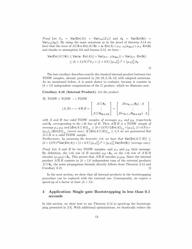
Proof. Let ϑA = Var(Err(A)) = Var(ϕs(ZA)) and ϑb = Var(Err(b)) =Var(ϕs(zb)). By using the same notations as in the proof of theorem 3.14 wehave that the error of Ab is Err(Ab) = u ·Err(A)+µA ·ϕs(εdec)+µA ·Err(b)and thanks to assumption 3.6 and lemma 3.12, we have :

Var(Err(A b)) ≤ Var(u · Err(A))) + Var(µA · ϕ(εdec)) + Var(µA · Err(b))≤ (k + 1)`Nβ2ϑA + (1 + kN) ‖µA‖22 ε2 + ‖µA‖22 ϑb.

ut

The last corollary describes exactly the classical internal product between twoTGSW samples, already presented in [10, 19, 3, 16, 14] with adapted notations.As we mentioned before, it is much slower to evaluate, because it consists in(k + 1)` independent computations of the product, which we illustrate now.

Corollary 3.16 (Internal Product). Let the product

: TGSW × TGSW −→ TGSW

(A,B) 7−→ AB =

A b1...

A b(k+1)`

=

Dech,β,ε(b1) ·A...

Dech,β,ε(b(k+1)`) ·A

,with A and B two valid TGSW samples of messages µA and µB respectivelyand bi corresponding to the i-th line of B. Then A B is a TGSW sample ofmessage µA·µB and ‖Err(AB)‖∞ ≤ (k+1)`Nβ ‖Err(A)‖∞+‖µA‖1 (1+kN)ε+‖µA‖1 ‖Err(B)‖∞ (worst case). If ‖Err(AB)‖∞ ≤ 1/4 we are guaranteed thatAB is a valid TGSW sample.Furthermore, by assuming the heuristic 3.6, we have that Var(Err(A B)) ≤(k+ 1)`Nβ2Var(Err(A)) + (1 + kN) ‖µA‖22 ε2 + ‖µA‖22 Var(Err(b)) (average case).

Proof. Let A and B be two TGSW samples, and µA and µB their message.By definition, the i-th row of B encodes µB • hi, so the i-th row of A Bencodes (µAµB) • hi. This proves that A B encodes µAµB . Since the internalproduct A B consists in (k + 1)` independent runs of the external productsA bi, the noise propagation formula directly follows from Theorem 3.14 andCorollary 3.15. ut

In the next section, we show that all internal products in the bootstrappingprocedure can be replaced with the external one. Consequently, we expect aspeed-up of a factor at least (k + 1)`.

4 Application: Single gate Bootstrapping in less than 0.1seconds

In this section, we show how to use Theorem 3.14 to speed-up the bootstrap-ping presented in [14]. With additional optimizations, we drastically reduce the

13

bootstrapping key size, and also reduce a bit the noise overhead. To bootstrap aLWE sample (a, b) ∈ Tn+1, which is rescaled as (a, b) mod 2N , using relevantencryptions of its secret key s ∈ Bn, the overall idea is the following. We startfrom a fixed polynomial testv ∈ TN [X], which is our phase detector: its i-th coef-ficient is set to the value that the bootstrapping should return if ϕs(a, b) = i/2N .The testv is first encoded in a trivial TLWE sample. Then, we iteratively rotateits coefficients, using external multiplications with TGSW encryptions of thehidden monomials X−siai . By doing so, the original testv gets rotated by the(hidden) phase of (a, b), and in the end, we simply extract the constant term asa LWE sample.

4.1 TLWE to LWE extraction

Like in previous work, extracting a LWE sample from a TLWE sample simplymeans rewriting polynomials into their list of coefficients, and discarding theN − 1 last coefficients of b. This yields a LWE encryption of the constant termof the initial polynomial message.

Definition 4.1 (TLWE Extraction). Let (a′′, b′′) be a TLWEs′′(µ) sam-ple with key s′′ ∈ Rk, We call KeyExtract(s′′) the integer vector s′ =(coefs(s′′1(X)), . . . , coefs(s′′k(X))) ∈ ZkN and SampleExtract(a′′, b′′) the LWEsample (a′, b′) ∈ TkN+1 where a′ = (coefs(a′′1(1/X)), . . . , coefs(a′′k(1/X))) andb′ = b′′0 the constant term of b′′. Then ϕs′(a

′, b′) (resp. msg(a′, b′)) is equal tothe constant term of ϕs′′(a

′′, b′′) (resp. to the constant term of µ = msg(a′′, b′′)).And ‖Err(a′, b′)‖∞ ≤ ‖Err(a′′, b′′)‖∞ and Var(Err(a′, b′)) ≤ Var(Err(a′′, b′′)).

4.2 LWE to LWE Key-Switching Procedure

Given a LWEs′ sample of a message µ ∈ T , the key switching procedure initiallyproposed in [9, 6] outputs a LWEs sample of the same µ without increasingthe noise too much. Contrary to previous exact keyswitch procedures, here wetolerate approximations.

Definition 4.2. Let s′ ∈ 0, 1n′ , s ∈ 0, 1n, a noise parameter γ ∈ R and aprecision parameter t ∈ N, we call key switching secret KSs′→s,γ,t a sequence offresh LWE samples KSi,j ∈ LWEs,γ(s′i · 2−j) for i ∈ [1, n′] and j ∈ [1, t].

Lemma 4.3 (Key switching). Given (a′, b′) ∈ LWEs′(µ) where s′ ∈ 0, 1n′with noise η′ = ‖Err(a′, b′)‖∞ and a keyswitching key KSs′→s,γ,t, where s ∈0, 1n, the key switching procedure outputs a LWE sample (a, b) ∈ LWEs(µ)where ‖Err(a, b)‖∞ ≤ η′ + n′tγ + n′2−(t+1).

14

Algorithm 2 KeySwitch procedure

Input: A LWE sample (a′ = (a′1, . . . , a′n′), b

′) ∈ LWEs′(µ), a keyswitching key KSs′→s

where s′ ∈ 0, 1n′, s ∈ 0, 1n and t ∈ N a precision parameter

Output: A LWE sample LWEs(µ)1: Let a′i be the closest multiple of 1

2t to a′i, thus |a′i − a′i| < 2−(t+1)

2: Binary decompose each a′i =∑tj=1 a

′i,j · 2−j where a′i,j ∈ 0, 1

3: Return (a, b) = (0, b′)−n′∑i=1

t∑j=1

a′i,j · KSi,j

Proof. We have

ϕs(a, b) = ϕs(0, b′)−n′∑i=1

t∑j=1

a′i,jϕs(KSi,j)

= b′ −n′∑i=1

t∑j=1

a′i,j

(2−js′i + Err(KSi,j)

)= b′ −

n′∑i=1

a′is′i −

n′∑i=1

t∑j=1

a′i,jErr(KSi,j)

= b′ −n′∑i=1

a′is′i −

n′∑i=1

t∑j=1

a′i,jErr(KSi,j) +

n′∑i=1

(a′i − a′i)s′i

= ϕs′(a′, b′)−

n′∑i=1

t∑j=1

a′i,jErr(KSi,j) +

n′∑i=1

(a′i − a′i)s′i.

The expectation of the left side of the equality is equal to msg(a, b). For theright side, each ai,j is uniformly distributed in 0, 1 and (a′i− a′i) is a 0-centeredvariable so the expectation of the sum is 0. Thus, msg(a, b) = msg(a′, b′). Weobtain ‖ϕs(a, b)−msg(a, b)‖∞ ≤ η′ + n′tγ + n′2−(t+1). utCorollary 4.4. Let t be an integer parameter. Under assumption 3.6, given(a′, b′) ∈ LWEs′(µ) with noise variance η′ = Var(Err(a′, b′)) and a key switchingkey KSs′→s,γ,`, the key switching procedure outputs an LWE sample (a′, b′) ∈LWEs(µ) where Var(Err(a, b)) ≤ η′ + n′tγ2 + n′2−2(t+1).

4.3 Bootstrapping Procedure

Given a LWE sample LWEs(µ) = (a, b), the bootstrapping procedure constructsan encryption of µ under the same key s but with a fixed amount of noise. Asin [14], we will use TLWE as an intermediate encryption scheme to perform ahomomorphic evaluation of the phase, but here we will use the external productfrom theorem 3.14 with a TGSW encryption of the key s.

Definition 4.5. Let s ∈ Bn, s′′ ∈ BN [X]k and α be a noise parameter. Wedefine the bootstrapping key BKs→s′′,α as the sequence of n TGSW sampleswhere BKi ∈ TGSWs′′,α(si).

15

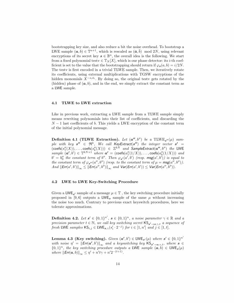
Algorithm 3 Bootstrapping procedure

Input: A LWE sample (a, b) ∈ LWEs,η(µ), a bootstrapping key BKs→s′′,α, a keyswitchkey KSs

′→s,γ where s′ = KeyExtract(s′′), two fixed messages µ0, µ1 ∈ T

Output: A LWE sample LWEs

(µ0 if ϕs(a, b) ∈

]− 1

4, 1

4

[;µ1 else

)1: Let µ = µ1+µ0

2and µ′ = µ0 − µ

2: Let b = b2Nbe and ai = b2Naie for each i ∈ [1, n]

3: Let testv := (1+X+ . . .+XN−1)×X−2N4 • µ′ ∈ TN [X]

4: ACC←(X b • (0, testv)

)∈ TN [X]k+1

5: for i = 1 to n6: ACC←

[h+ (X−ai − 1) • BKi

] ACC

7: Let u := (0, µ) + SampleExtract(ACC)8: Return KeySwitchKS(u)

We first provide a comparison between the bootstrapping of Algorithm 3and [14, Algorithm 1,2] proposal.

– Like [14], we rescale the computation of the phase of the input LWE sampleso that it is modulo 2N (line 2) and we map all the corresponding operationsin the multiplicative cyclic group 1, X, . . . ,X2N−1. Since our LWE samplesare described over the real torus, the rescaling is done explicitly in line 2.This rescaling may induce a cumulated rounding error of amplitude at mostδ ≈ √n/4N in the average case and δ ≤ (n + 1)/4N in the worst case.In the best case, this amplitude can even be zero (δ = 0) if in the actualrepresentation of LWE samples, all the coefficients are restricted to multipleof 1

2N , which would be the analogue of [14]’s setting.– As in [14], messages are encoded as roots of unity in R. Our accumulator

is a TLWE sample instead of a TGSW sample in [14]. Also accumulatoroperations use the external product from Theorem 3.14 instead of the slowerclassical internal product. The test vector (1+X+ . . .+XN−1) is embeddedin the accumulator from the very start, when the accumulator is still noiselesswhile in [14], it is added at the very end. This removes a factor

√N to the

final noise overhead.– All the TGSW ciphertexts of X−aisi required to update the accumulator

internal value are computed dynamically as a very small polynomial combi-nation of BKi in the for loop (line 5). This completely removes the need todecompose each ai on an additional base Br, and to precompute all possibil-ities in the bootstrapping key. In other words, this makes our bootstrappingkey 46 times smaller than in [14], for the exact same noise overhead. Besides,due to this squashing technique, two accumulator operations were performedper iteration instead of one in our case. This gives us an additional 2× speedup.

Theorem 4.6 (Bootstrapping Theorem). Let h ∈ M`(k+1),k+1(TN [X]) bethe gadget defined in Equation 1 and let Dech,ε,β be the associated vector gadgetdecomposition function.

16

Let s ∈ Bn, s′′ ∈ BN [X]k and α, γ be noise amplitudes. Let BK = BKs→s′′,α

be a bootstrapping key, let s′ = KeyExtract(s′′) ∈ BkN and KS = KSs′→s,γ,t be akeyswitching secret.

Given (a, b) ∈ LWEs(µ) for µ ∈ T, two fixed messages µ0, µ1, Algorithm 3outputs a sample in LWEs(µ′) s.t. µ′ = µ0 if |ϕs(a, b)| < −1/4− δ and µ′ = µ1

if |ϕs(a, b)| > 1/4 + δ where δ is the cumulated rounding error equal to n+14N in

the worst case and δ = 0 if the all coefficients of (a, b) are multiple of 12N . Let

v be the output of Algorithm 3. Then ‖Err(v)‖∞ ≤ 2n(k + 1)`βNα + kNtγ +n(1 + kN)ε+ kN2−(t+1).

Proof. Line 1: the division by two over torus gives two possible values for (µ, µ′).In both cases, µ+ µ′ = µ0 and µ− µ′ = µ1.

Line 2: let ϕdef= b−∑n

i=1 aisi mod 2N . We have∣∣∣ϕ− ϕ

2N

∣∣∣ = b− b2Nbe2N

+

n∑i=1

(ai −

b2Naie2N

)si ≤

1

4N+

n∑i=1

1

4N≤ n+ 1

4N. (2)

And if the coefficients (a, b) ∈ 12NZ/Z, then ϕ = ϕ

2N . In all cases, |ϕ− ϕ2N | < δ.

At line 3, the test vector testv := (1+X+ . . .+XN−1) ·X− 2N4 • µ′ is defined

such that for all p ∈ [0, 2N ], the constant term of Xp • testv is either µ′ ifp ∈]]− N

2 ,N2 [[ and −µ′ else.

In the loop for (from line 5 to 6), we will prove the following invariant: At thebeginning of iteration i+1 ∈ [1, n+1] (i.e. at the end of iteration i), msg(ACCi) =

Xb−∑i

j=1 ajsj • testv and ‖Err(ACCi)‖∞ ≤∑ij=1

(2(k + 1)`Nβ ‖Err(BKj)‖∞ +

(1 + kN)ε)

.

At the beginning of iteration i = 1, the accumulator contains a trivial ci-

phertext msg(ACC1) =(X b • testv

), so ‖Err(ACC1)‖∞ = 0.

During iteration i, Ai = h+ (X−ai − 1) •BKi is a TGSW sample of messageX−aisi (this can be seen by replacing si with its two possible values 0 and 1) andof noise ‖Err(Ai)‖∞ ≤ 2 ‖Err(BKi)‖∞. This inequality holds from lemma 3.11.Then, we have:

msg(ACCi) = msg(Ai ACCi−1

)= msg

(Ai

)•msg(ACCi−1) (from Theorem 3.14)

= X−aisi · (Xb−∑i−1

j=1 ajsj • testv)

and from the norm inequality of Theorem 3.14,

‖Err(ACCi)‖∞ ≤ (k + 1)`Nβ ‖Err(Ai)‖∞ + ‖msg(Ai)‖1 (1 + kN)ε+

+ ‖msg(Ai)‖1 ‖Err(ACCi−1)‖∞≤ (k + 1)`Nβ2 ‖Err(BKi)‖∞ + (1 + kN)ε+ ‖Err(ACCi−1)‖∞ .

17

This proves the invariant by induction on i.

After SampleExtract (line 7), the message of u is equal to the constantterm of the message of ACCn, i.e. Xϕ • testv where ϕ = b − ∑n

i=1 aisi. Ifϕ ∈ [[−N/2, N/2[[, the constant term is equal to µ′ and −µ′ otherwise.

In other words, |ϕs(a, b)| < 1/4− δ, then ϕs(a, b) < 1/4− δ and ϕs(a, b) ≥−1/4+δ and thus using Equation (2), we obtain that ϕ ∈]]− N

2 ,N2 [[ and thus, the

message of u is equal to µ′. And if |ϕs(a, b)| > 1/4 + δ then ϕs(a, b) > 1/4 + δor ϕs(a, b) < −1/4 − δ and using Equation (2), we obtain the message of u isequal to −µ′.

Since SampleExtract does not add extra noise, ‖Err(u)‖∞ ≤ ‖Err(ACCn)‖.Since the KeySwitch procedure preserves the message, the message of v =KeySwitchKS(u) is equal to the message of u. And ‖Err(v)‖∞ ≤ ‖Err(u)‖∞ +kNtγ + kN2−(t+1). utCorollary 4.7. Let ϑBK = Var(Err(BKi)) = 2/π ·α2 and VKS = Var(Err(KSi)) =2/π · γ2. Under the same conditions of Theorem 4.6, and assuming Assump-tion 3.6, then the Variance of the output v of Algorithm 3 satisfies Var(Err(v)) ≤2Nn(k + 1)`β2ϑBK + kNtVKS + n(1 + kN)ε2 + kN2−2(t+1).

Proof. The proof is the same as for the proof of the bound on ‖Err(v)‖∞ replacingall ‖‖∞ inequalities by Var() inequalities. ut

4.4 Application to circuits

In [14], the homomorphic evaluation of a NAND gate between LWE samplesis achieved with 2 additions (one with a noiseless trivial sample) and a boot-strapping. Let BK = BKs→s′′,α be a bootstrapping key and KS = KSs′→s,γ,t

be a keyswitching secret defined as in thm. 4.6 such that 2n(k + 1)`βNα +kNtγ + n(1 + kN)ε + kN2−(t+1) < 1

16 , We denote as Bootstrap (c) the out-put of the bootstrapping procedure described in Algorithm 3 applied to c withµ0 = 0 and µ1 = 1

4 . Let consider two LWE samples c1 and c2, with mes-sage space 0, 1/4 and ‖Err(c1)‖∞ , ‖Err(c2)‖∞ ≤ 1

16 . The result is obtainedby computing c = (0, 5

8 )-c1-c2, plus a bootstrapping. Indeed the possible val-ues for the messages of c are 5

8 ,38 if either c1 or c2 encode 0, and 1

8 if bothencode 1

4 . Since the noise amplitude ‖Err(c)‖∞ is < 18 , then |ϕs(c)| > 1

4 iff.NAND(msg(c1),msg(c2)) = 1. This explains why it suffices to bootstrap c withparameters (µ1, µ0) = ( 1

4 , 0) to get the answer. By using a similar approach, itis possible to directly evaluate with a single bootstrapping all the basic gates:

– HomNOT(c) = (0, 14 )-c (no bootstrapping is needed);

– HomAND(c1, c2) = Bootstrap((0,− 1

8 )+c1+c2);

– HomNAND(c1, c2) = Bootstrap((0, 5

8 )-c1-c2);

– HomOR(c1, c2) = Bootstrap((0, 1

8 )+c1+c2);

– HomXOR(c1, c2) = Bootstrap (2 · (c1-c2)).

The HomXOR(c1, c2) gate can be achieved also by performingBootstrap (2 · (c1+c2)).

18

4.5 Parameters Implementation and Timings

In this section, we review our implementation parameters and provide a com-parison with previous works.

Samples. From a theoretical point of view, our scale invariant scheme is definedover the real torus T, where all the operations are modulo 1. In practice, sincewe can work with approximations, we chose to rescale the elements over T by afactor 232, and to map them to 32-bit integers. Thus, we take advantage of thenative and automatic mod 232 operations, including for the external multipli-cation with integers. Except for some FFT operations, this seems more stableand efficient than working with floating point numbers and reducing modulo 1regularly. Polynomials mod XN + 1 are either represented as the classical list ofthe N coefficients, either using the Lagrange half-complex representation, whichconsists in the complex (2 · 64bits) evaluations of the polynomial over the rootsof unity exp(i(2j + 1)π/N) for j ∈ [[0, N2 [[. Indeed, the N

2 other evaluations arethe conjugates of the first ones, and do not need to be stored. The conversionbetween both representations is done via Fast Fourier Transform (FFT) (usingthe library FFTW [15], also used by [14]). Note that the direct FFT transform is√

2N lipschitzian, so the lagrange half-complex representation tolerates approx-imations, and 53bits of precision is indeed more than enough, provided that thereal representative remains small. However, the modulo 1 that can reduce thecoefficients of Torus polynomials cannot be applied from the Lagrange repre-sentation: we need to perform regular transformations to and from the classicalrepresentation. Luckily, it does not represent an overhead, since these conversionsare needed anyway, at each iteration of the bootstrapping in order to decomposethe accumulator in base h.

Parameters. We take the same or even stronger security parameters as [14], butwe adapt them to our notations. We used n = 500, N = 1024, k = 1.

– LWE samples: 32 · (n+ 1) bits ≈ 2 KBytes.The mask of all LWE samples (initial and KeySwitch) are clamped to multi-ples of 1

2048 . Therefore, the phase computation in the bootstrapping is exact(δ = 0).

– TLWE samples: (k + 1) ·N · 32 bits ≈ 8 KBytes.– TGSW samples: (k + 1) · ` TLWE samples ≈ 48 KBytes.

To define h and Dech,β,ε, we used ` = 3, Bg = 1024, so β = 512 and ε = 2−31.– Bootstrapping Key: n TGSW samples ≈ 23.4 MBytes.

We used α = 9.0 ·10−9. Since we have a lower noise overhead, our parameteris higher than the parameter ≈ 3.25 ·10−10 of [14], (i.e. ours is more secure),but in counterpart, our TLWE key is binary. See Section 6 for more detailson the security analysis.

– Key Switching Key: k ·N · t LWE samples ≈ 29.2 MBytes.we used γ = 3.05 · 10−5, t = 15 (The decomposition in the key switching hasprecision 2−16).

19

– Correctness: The final error variance after bootstrapping is 9.24.10−6, byCorollary 4.7. It corresponds to a standard deviation of σ = 0.00961.In [14], the final standard deviation is larger 0.01076. In other words, thenoise amplitude after our bootstrapping is < 1

16 with very high probability

erf(1/16√

2σ) ≥ 1 − 2−33.56 (this is comparable to probability ≥ 1 − 2−32

in [14]).

Note that the size of the key switching key can be reduced by a factorn + 1 = 501 if all the masks are the output of a pseudo random function;we may for instance just give the seed. The same technique can be applied tothe bootstrapping key, on which the size is only reduced by a factor k + 1 = 2.

Implementation tools and Source Code. The source code of our implementation isavailable on github https://github.com/tfhe/tfhe. We implemented the FHEscheme in C/C++, and run the bootstrapping algorithm on a 64-bit single core(i7-4930MX) at 3.00GHz. This seems to correspond to the machine used in [14].We implemented a version with classical representation for polynomials, and aversion in Lagrange half-complex representation. The following table comparesthe number of multiplications or FFT that are required to complete one externalproduct and the full bootstrapping.

#(Classical products) #(FFT + Lagrange repr.)External product 12 8

Bootstrapping 6000 4006

Bootstrapping in [14] (72000) 48000

In practice, we obtained a running time of 52ms per bootstrapping usingthe Lagrange half-complex representation. It is coherent with the 12x speed-uppredicted by the table. Profiling the execution shows that the FFTs and complexmultiplications are still taking more than 90% of the total time. Other operationslike keyswitch have a negligible running time compared to the main loop of thebootstrapping.

5 Leveled Homomorphic encryption

In the previous section, we showed how to accelerate the bootstrapping com-putation in FHE. In this section, we focus on the improvement of Leveled Ho-momorphic encryption schemes. We present an efficient way to evaluate anydeterministic automata homomorphically.

5.1 Boolean circuits interpretation

In order to express our external product in a circuit, we consider two kindsof wires: control wires which encode either a small integer or a small integerpolynomial. They will be represented by a TGSW sample; and data wires whichencode either a sample in T or in TN [X]. They will be represented by a TLWE

20

sample. The gates we present contain three kinds of slots: control input, datainput and data output. In this following section, the rule to build valid circuitsis that all control wires are freshly generated by the user, and the data inputports of our gates can be either freshly generated or connected to a data outputor to another gate.

We now give an interpretation of our leveled scheme, to simulate booleancircuits only. In this case, the message space of the input TLWE samples will berestricted to 0, 1

2, and the message space of control gates to 0, 1.

– The constant source Cst(µ) for µ ∈ 0, 12 is defined with a single data

output equal to (0, µ).

– The negation gate Not(d) takes a single data input d and outputs (0, 12 )−d.

– The controlled And gate CAnd(C,d) takes one control input C and one datainput d, and outputs C d.

– The controlled Mux gate CMux(C,d1,d0) takes one control input C and twodata inputs d1,d0 and returns C (d1 − d0) + d0.

Unlike classical circuits, these gates have to be composed with each otherdepending on the type of inputs/outputs. In our applications, the TGSW en-cryptions are always fresh ciphertexts.

µT-LWE (trivial)µ

0 0

µd12 − µd

T-LWET-LWEη η

µC

T-LWE

T-GSW

µd

µC · µd

T-LWE

ηC

ηd

ηd +O(ηC)

µC

T-LWE

T-GSW

µd0

µC · (µd1 − µd0) + µd0

T-LWE

µd1

T-LWE 1

0

ηC

ηd1

ηd0

max(ηd1 , ηd0) +O(ηC)

Theorem 5.1 (Correctness). Let µ ∈ 0, 12, d,d1,d0 ∈ TLWEs(0, 1

2) andC ∈ TGSWs(0, 1).

– msg(Cst(µ)) = µ

– msg(Not(d)) = 12 − µ = not µ

– msg(CAnd(C,d)) = msg(C) ·msg(d)

– msg(CMux(C,d1,d0)) = msg(C)?msg(d1):msg(d0)

Theorem 5.2 (Worst-case noise). In the conditions of thm 5.1, we have

– ‖Err(Cst(µ))‖∞ = 0

– ‖Err(Not(d))‖∞ = ‖Err(d)‖∞– ‖Err(CAnd(C,d))‖∞ ≤ ‖Err(d)‖∞ + η(C)

– ‖Err(CMux(C,d1,d0))‖∞ ≤ max(‖Err(d0)‖∞ , ‖Err(d1)‖∞) + η(C),

where η(C) = (k + 1)`Nβ ‖Err(C)‖∞ + (kN + 1)ε.

21

Proof. The noise is indeed null for constant gates, and negated for the Not gate,which preserves the norm. The noise bound for the CAnd gate is exactly the onefrom Theorem 3.14, however, we need to explain why there is a max in the CMuxformula instead of the sum we would obtain by blindly applying thm 3.14. Letd = d1 − d0, recall that in the proof of Theorem 3.14, the expression of C dis Dech,β,ε(d) • zC + µCεdec + µCzd + (0, µC · µd), where C = zC + µC · h andd = zd + µd, zC and zd are respectively TGSW and TLWE samples of 0, and‖εdec‖∞ ≤ ε. Thus, CMux(C,d1,d0) is the sum of four terms:

– Dech,β,ε(d) • zC of norm ≤ (k + 1)`NβηC ;– µCεdec of norm ≤ (kN + 1)ε;– zd0 +µC(zd1 − zd0), which is either zd1 or zd0 , depending on the value of µC ;– µd0 + µC · (µd1 − µd0), which is the output message µC?µd1 :µd0 , and is not

part of the noise.

Thus, summing the three terms concludes the proof. ut

Corollary 5.3 (Average noise of boolean gates). In the conditions ofthm 5.1, and in the conditions of Assumption 3.6, we have:

– Var(Err(Cst(µ))) = 0;– Var(Err(Not(d))) = Var(Err(d));– Var(Err(CAnd(C,d))) ≤ Var(Err(d)) + ϑ(C);– Var(Err(CMux(C,d1,d0))) ≤ max(Var(Err(d0)),Var(Err(d1))) + ϑ(C),

where ϑ(C) = (k + 1)`Nβ2Var(Err(C)) + (kN + 1)ε2.

Proof. Same as thm 5.2, replacing all norm inequalities by Variance inequalities.ut

We now obtain theorems which are analogue to [16], with a bit less noise onthe mux gate, but with the additional restriction that CAnd and CMux have acontrol wire, which must necessarily be a fresh TGSW ciphertext.

The next step is to understand the meaning of this additional restriction interms of expressiveness of the resulting homomorphic circuits.

It is clear that we cannot build a random boolean circuit, and just apply thenoise recurrence formula from theorem 5.2 or cor. 5.3 to get the output noiselevel. Indeed, it is not allowed to connect a data wire to an control input.

In the following section, we will show that we can still obtain the two mostimportant circuits of [16], namely the deterministic automata circuits, which canevaluate any permutation of regular languages with noise propagation sublinearin the word length and the lookup table, which evaluates arbitrary functionswith sublinear noise propagation.

Interestingly, these circuits were historically obtained in [20, 10, 16] with theinternal product of GSW, as an optimization which takes advantage of the un-balanced coefficients in the noise recurrence formula. Here, it appears that theexternal product forces us to use these optimal circuits, because it is the onlyway to connect the wires.

22

5.2 Deterministic automata

It is folklore that every deterministic program which reads its input bit-by-bitin a pre-determined order, uses less than B bits of memory, and produces aboolean answer, is equivalent to a deterministic automata of at most 2B states(independently of the time complexity). This is in particular the case for everyboolean function of p variables, that can be trivially executed with p − 1 bitsof internal memory by reading and storing its input bit-by-bit before returningthe final answer. It is of particular interest for most arithmetic functions, likeaddition, multiplication, or CRT operations, whose naive evaluation only requiresO(log(p)) bits of internal memory.

Let A = (Q, i, T0, T1, F ) be a deterministic automata (over the alphabet0, 1, where Q is the set of states, i ∈ Q denotes the initial state, T0, T1

are the two transitions (deterministic) functions from Q to Q and F ⊂ Q isthe set of final states. Such automata is used to evaluate (rational) booleanfunctions on words where the image of (w1, . . . , wp) ∈ Bp is equal to 1 iff.Twp

(Twp−1(. . . (Tw1

(i)))) ∈ F , and 0 otherwise.Following the construction of [16], we show that we are able to evaluate any

deterministic automata homomorphically using only constant and CMux gatesefficiently. The noise propagation remains linear in the length of the word w, butcompared to [16, Thm. 7.11], we reduce the number of evaluated CMux gates bya factor |w| for a specific class of acyclic automata that are linked to fixed-timealgorithms.

Theorem 5.4 (Evaluating Deterministic Automata). Let A =(Q, i, T0, T1, F ) be a deterministic automata. Given p valid TGSW sam-ples C1, . . . , Cp encrypting the bits of a word w ∈ Bp, with noise amplitudeη = maxi ‖Err(Ci)‖∞ and ϑ = maxi Var(Err(Ci)), by evaluating at most ≤ p#QCmux gates, one can produce a TLWE sample d which encrypts 1

2 iff A acceptsw, and 0 otherwise such that ‖Err(d)‖∞ ≤ p · ((k + 1)`Nβη + (kN + 1)ε).Assuming Heuristic 3.6, Var(Err(d)) ≤ p · ((k + 1)`Nβ2ϑ + (kN + 1)ε2).Furthermore, the number of evaluated CMux can be decreased to ≤ #Q. if Asatisfies either one of the conditions:(i) for all q ∈ Q (except KO states), all the words that connect i to q have thesame length;(ii) A only accepts words of the same length.

Proof. We initialize #Q noiseless ciphertexts dq,p for q ∈ Q with dq,p = (0, 12 ) =

Cst( 12 ) if q ∈ F and dq,p = (0, 0) = Cst(0) otherwise. Then for each letter of

w, we map the transitions as follow for all q ∈ Q an j ∈ [[0, p − 1]]: dq,j−1 =CMux(Cj ,dT1(q),j ,dT0(q),j). And we finally output di,0.

Indeed, with this construction, we have

msg(di,0) = msg(dTw1(i),1) = . . . = msg(dTwp(Twp−1

...(Tw1(i))...),p),

which encrypts 12 iff Twp

(Twp−1. . . (Tw1

(i)) . . .) ∈ F , i.e. iff w1 . . . wp is acceptedby A. This proves correctness.

23

For the complexity, each dq,j for all q ∈ Q an j ∈ [[0, p− 1]] is computed witha single CMux. By applying the noise propagation inequalities of Theorem 5.2and Corollary 5.3, it follows by an immediate induction on j from p down to 0,that for all j ∈ [[0, p]], ‖Err(dq,j)‖∞ ≤ (p − j) · ((k + 1)`Nβη + (kN + 1)ε) andVar(Err(dq,j)) ≤ (p− j) · ((k + 1)`Nβ2ϑ+ (kN + 1)ε2).

Note that it is sufficient to evaluate only the dq,j when q is accessible by atleast one word of length j. Thus, if the A satisfies the additional condition (i),then for each q ∈ Q, we only need to evaluate dq,j for at most one position j.Thus, we evaluate less than #Q CMux gates in total.

Finally, if A satisfies (ii), then we first compute the minimal deterministicautomata of the same language (and removing the KO state if it is present),then with an immediate proof by contradiction, this minimal automata satisfies(i), and has less than #Q states. ut

For sake of completeness, since every boolean function with p variables canbe evaluated by an Automata (that accepting only words of length p), we obtainthe evaluation of arbitrary boolean function as an immediate corollary, which isthe leveled variant of [16, Cor 7.9].

Lemma 5.5 (Arbitrary Functions). Let f be any boolean function with pinputs, and c1, . . . , cp be p TGSWs(0, 1) ciphertexts of x1, . . . , xp ∈ 0, 1,with noise ‖Err(ci)‖∞ ≤ η for all i ∈ [1, p]. Then the CMux-based ReducedBinary Decision Diagram of f computes a TLWEs ciphertext d of 1

2f(x1, . . . , xp)with noise ‖Err(d)‖∞ ≤ p((k + 1)`Nβη + (kN + 1)ε) by evaluating N (f) ≤ 2p

CMux gates where N (f) is the number of distinct partial functions (xl, . . . , xp)→f(x1, . . . , xp) for all l ∈ [[1, p+ 1]], (x1, . . . , xl−1) ∈ Bl−1.

Proof (sketch). A trivial automata which evaluates f consists in its full binarydecision tree, with the initial state i = q0,0 as the root, each state ql,j depthl ∈ [[0, p−1]] and j ∈ [[0, 2l−1]] is connected with T0(ql,j) = ql+1,2j and T1(ql,j) =ql+1,2j+1, and at depth p, qp,j ∈ F iff f(x1, . . . , xp) = 1 where j =

∑pl=1 xl2

p−l.The minimal version of this automaton has at most N (f) states, the rest followsfrom Theorem 5.4. ut

Application: compilation for leveled homomorphic circuits We now givean example of how we can map a problem to an automata in order to perform aleveled homomorphic evaluation. We will illustrate this concept on the compu-tation of the p-th bit of an integer product a× b where a and b are given in base2. We do not claim that the automata approach is the fastest way to solve theproblem, arithmetic circuits based on bitDecomp/recomposition are likely to befaster. But the goal is to clarify the generality and simplicity of the process. Allwe need is a fixed-time algorithm that solves the problem using the least possiblememory. Among all algorithms that compute a product, the most naive ones arein general the best: here, we choose the elementary-school multiplication algo-rithm that computes the product bit-by-bit, starting from the LSB, and countingthe current carry with the fingers. The pseudocode of this algorithm is recalled

24

in Algorithm 4. The pseudo-code is almost given as a deterministic automata,since each step reads a single input bit, and uses it to update its internal state(x, y), that can be stored in only M = log2(4p) bits of memory. More precisely,the states Q of the corresponding automata A would be all (j, (x, y)) wherej ∈ [[0, jmax]] is the step number (i.e. number of reads from the beginning) and(x, y) ∈ B× [[0, 2p[[ are the 4p possible values of the internal memory. The initialstate is (0, 0, 0), the total number of reads jmax is ≤ p2, and the final states areall (jmax, x, y) where y is odd. This automata satisfies condition (i), since a state(j, x, y) can only be reached after reading j inputs, so by theorem Thm.5.4, theoutput can be homomorphically computed by evaluating less than #Q ≤ 4p3

CMux gates, with some O(p) noise overhead. The number of Mux can decreaseby a factor 8 by minimizing the automata. Using the same parameters as thebootstrapping key, for p = 32, evaluating one Mux gate takes about 0.0002s, sothe whole program (16384 Cmux) would be homomorphically evaluated in 3.2seconds.

We mapped a problem from its high-level description to an algorithm usingvery few bits of memory. Since low memory programs are in general more naive,it should be easier to find them than obtaining a circuit with low multiplicativedepth that would be required for other schemes such as BGV, FHE over integers.Once a suitable program is found, as in the previous example, compiling it to anet-list of CMux gates is straightforward by our Theorem 5.4.

Algorithm 4 elementary fixed time algorithm that computes the p-th bit of theproduct of a and b

Input: a and b as little endian bitsOutput: p-th bit of ab1: Internal memory: x ∈ 0, 1, y ∈ [[0, 2p[[2: initialize x = 0, y = 03: for k = 0 to p− 1 do4: for i = 0 to k − 1 do5: read ai; x = ai6: read bk−i; y = y + xbk−i7: end for8: read ak; x = ak9: read b0; y = b(y + xb0)/2c

10: end for11: for i = 0 to p do12: read ai; x = ai13: read bp−i; y = y + xbp−i14: end for15: accept if y == 1 mod 2

25

6 Practical security parameters

For an asymptotical security analysis, since the phase is lipschitzian, TLWEsamples can be equivalently mapped to their closest binLWE (or bin-RingLWE),which in turn can be reduced to standard LWE/ringLWE with full secret usingthe modulus-dimension reduction [7] or group-switching techniques [16]. It canthen be reduced to worst case BDD instances. It is also easy to write a directand tighter search-to-decision reductions for TLWE, or a direct worst-case toaverage-case reductions from TLWE to Gap-SVP or BDD.

In this section, we will rather focus on the practical hardness of LWE, andexpress after all the security parameter λ directly as a function of the entropyof the secret n and the error rate α.

Our analysis is based on the work described in [2]. This paper studies manyattacks against LWE, ranging from a direct BDD approach with standard lat-tice reduction, sieving, or with a variant of BKW [5], resolution via man in themiddle attacks. Unfortunately, they found out that there is no single-best at-tack. According to their results table [2, Section 8, Tables 7,8] for the range ofdimensions and noise used for FHE, it seems that the SIS-distinguisher attackis often the best candidate (related to the Lindner-Peikert [21] model, and alsoused in the parameter estimation of [14]). However, since q is not a parameter inour definition of TLWE, we need to adapt their results. This section relies on thefollowing heuristics concerning the experimental behaviour of lattice reductionalgorithms. They have been extensively verified and used in practice.

1. The fastest lattice reduction algorithms in practice are blockwise lattice al-gorithms (like BKZ-2.0[11], D-BKZ [24], or the slide reduction with largeblocksize [17, 24]).

2. Practical blockwise lattice reduction algorithms have an intrinsic qualityδ > 1 (which depends on the blocksize), and given a m-dimensional realbasis B of volume V , they compute short vectors of norm δmV 1/m.

3. The running time of BKZ-2.0 (expressed in bit operations) as a function ofthe quality parameter is: log2(tBKZ)(δ) = 0.009

log2(δ)2 − 27 (According to the

extrapolation by Albrecht et al [1] of Liu-Nguyen datasets [22]).

4. The coordinates of vectors produced by lattice reduction algorithms are bal-anced. Namely, if the algorithm produces vectors of norm ‖v‖2, each coeffi-cient has a marginal Gaussian distribution of standard deviation ‖v‖2 /

√n.

Provided that the geometry of the lattice is not too skewed in particulardirections, this fact can sometimes be proved, especially if the reduction al-gorithm samples vectors with Gaussian distribution over the input lattice.This simple fact is at the heart of many attacks based on Coppersmith tech-niques with lattices.

5. For mid-range dimensions and polynomially small noise, the SIS-distinguisher plus lattice reduction algorithms combined with the search-to-decision is the best attack against LWE; (but this point is less clear,

26

according to the analysis of [1], at least, this attack model tends to over-estimate the power of the attacker, so it should produce more conservativeparameters).

6. Except for small polynomial speedups in the dimension, we don’t know betteralgorithms to find short vectors in random anti-circulant lattices than genericalgorithms. This folklore assumption seems still up-to date at the time ofwriting.

If one finds a small integer combination that cancels the mask of homogeneousLWE samples, one may use it to distinguish them from uniformly chosen randomsamples. If this distinguisher has small advantage ε, we repeat it about 1/ε2

times. Then, thanks to the search to decision reduction (which is particularlytight with our TLWE formulation), each successful answer of the distinguisherreveals one secret key bit. To handle the continuous torus, and since q is nota parameter of TLWE either, we show how to extend the analysis of [2] to ourscheme.

Let (a1, b1), . . . , (am, bm) be either m LWE samples of parameter α or m uni-formly random samples of Tn+1, we need to find a small combination v1, . . . , vmof samples such that

∑viai is small. This condition differs from most previous

models, were working on a discrete group, and required an exact solution. By al-lowing approximations, we may find solutions for much smaller m than the usualbound n log q, even m < n can be valid. Now, consider the (m+n)-dimensionallattice, generated by the rows of the following basis B ∈Mn+m,n+m(R):

B =

1 0

. . . 00 1

a1,1 · · · a1,n 1 0...

. . ....

. . .

am,1 · · · am,n 0 1

.

Our target is to find a short vector w = [x1, . . . , xn, v1, . . . , vm] in the latticeof B, whose first n coordinates (x1, . . . , xn) =

∑mi=1 viai mod 1 are shorter

than the second part (v1, . . . , vm). To take this skewness into account, we choosea real parameter q > 1 (that will be optimized later), and apply the unitarytransformation fq to the lattice, which multiplies the first n coordinates by qand the last m coordinates by 1/qn/m. Although this matrix looks like a classicalLWE matrix instance, the variable q is a real parameter, and it doesn’t needto be an integer. It then suffices to find a regular short vector with balancedcoordinates in the transformed lattice, defined by this basis:

27

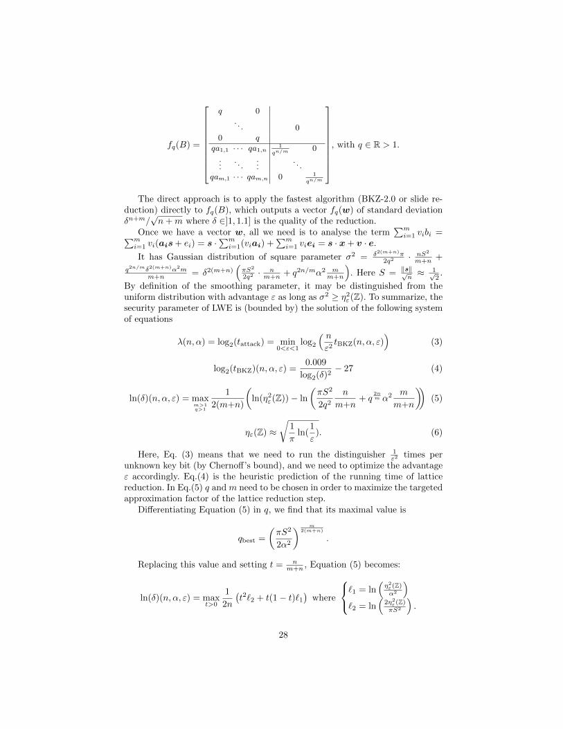
fq(B) =

q 0

. . . 00 q

qa1,1 · · · qa1,n1

qn/m 0

.... . .

.... . .

qam,1 · · · qam,n 0 1

qn/m

, with q ∈ R > 1.

The direct approach is to apply the fastest algorithm (BKZ-2.0 or slide re-duction) directly to fq(B), which outputs a vector fq(w) of standard deviationδn+m/

√n+m where δ ∈]1, 1.1] is the quality of the reduction.

Once we have a vector w, all we need is to analyse the term∑mi=1 vibi =∑m

i=1 vi(ais+ ei) = s ·∑mi=1(viai) +

∑mi=1 viei = s · x+ v · e.

It has Gaussian distribution of square parameter σ2 = δ2(m+n)π2q2 · nS2

m+n +

q2n/mδ2(m+n)α2mm+n = δ2(m+n)

(πS2

2q2 · nm+n + q2n/mα2 m

m+n

). Here S = ‖s‖√

n≈ 1√

2.

By definition of the smoothing parameter, it may be distinguished from theuniform distribution with advantage ε as long as σ2 ≥ η2

ε(Z). To summarize, thesecurity parameter of LWE is (bounded by) the solution of the following systemof equations

λ(n, α) = log2(tattack) = min0<ε<1

log2

( nε2tBKZ(n, α, ε)

)(3)

log2(tBKZ)(n, α, ε) =0.009

log2(δ)2− 27 (4)

ln(δ)(n, α, ε) = maxm>1q>1

1

2(m+n)

(ln(η2

ε(Z))− ln

(πS2

2q2

n

m+n+ q

2nm α2 m

m+n

))(5)

ηε(Z) ≈√

1

πln(

1

ε). (6)

Here, Eq. (3) means that we need to run the distinguisher 1ε2 times per

unknown key bit (by Chernoff’s bound), and we need to optimize the advantageε accordingly. Eq.(4) is the heuristic prediction of the running time of latticereduction. In Eq.(5) q and m need to be chosen in order to maximize the targetedapproximation factor of the lattice reduction step.

Differentiating Equation (5) in q, we find that its maximal value is

qbest =

(πS2

2α2

) m2(m+n)

.

Replacing this value and setting t = nm+n , Equation (5) becomes:

ln(δ)(n, α, ε) = maxt>0

1

2n

(t2`2 + t(1− t)`1

)where

`1 = ln(η2ε(Z)α2

)`2 = ln

(2η2ε(Z)πS2

).

28

Finally, by differentiating this new expression in t, the maximum of δ isreached for tbest = `1

2(`1−`2) , because `1 > `2, which gives the best choices of m

and q and δ. Finally, we optimize ε numerically in Eq.(3).All previous results are summarized in Figure 6, which displays the security

parameter λ as a function of n, log2(α).

Fig. 1. Security parameter λ as a function of n and α for LWE samples

0

5

10

15

20

25

30

35

40

45

0 200 400 600 800 1000

log

2(1

/α)

n

Values of λ(n,α)

32

64

128

256

512

51

2

384

256

192

128

80

40

Switch Key

Boot. Key

Boot. Key [11]

This curve shows the security parameter levels λ (black levels) as a function of n = kN(along the x-axis) and log2(1/α) (along the y-axis) for TLWE (also holds for bin-LWE),considering both the attack of this section and the collision attack in time 2n/2.

In particular, in the following table we precise the values for the keyswitchingkey and the bootstrapping key (for our implementation and for the one in [14]).

n α λ εbest mbest qbest δbest

Switch key 500 2−15 136 2−12 444 125.7 1.0058Boot. key 1024 9.0 · 10−9 194 2−10 968 7664. 1.0048

Boot.key, [14] 1024 3.25 · 10−10 141 2−7 993 44096 1.0055

The table shows that the strength of the lattice reduction is compatiblewith the values announced in [14]. Our model predicts that the lattice reductionphase is harder (δ = 1.0055 in our analysis and δ = 1.0064 in [14]), but thevalue of ε is bigger in our case. Overall, the security of their parameters-setis evaluated by our model to 136-bits of security, which is larger than the≥ 100-bits of security announced in [14]. The main reason is that we take intoaccount the number of times we need to run the SIS-distinguisher to obtaina non negligible advantage. Since our scheme has a smaller noise propagation

29

overhead, we were able to raise the input noise levels in order to strengthenthe system, so with the parameters we chose in our implementation, our modelpredicts 194-bits of security for the bootstrapping key and 136-bits for thekeyswitching key (which remains the bottleneck).

7 Conclusion

In this paper, we presented a generalization of the LWE and GSW homomorphicencryption schemes. We improved the execution timing of the bootstrappingprocedure and we reduced the size of the keys by keeping at least the samesecurity as in previous fast implementations. This result has been obtained bysimplifying the multiplication morphism, which is the main operation used inthe scheme we described. As a proof of concept we implemented the schemeitself and we gave concrete parameters and timings. Furthermore, we extend theapplicability of the external product to leveled homomorphic encryption. Wefinally gave a detailed security analysis. Now the main drawback to make ourscheme adapted for real life applications is the expansion factor of the ciphertextsof around 400000 with fairly limited batching capabilities.

Acknowledgements This work has been supported in part by the CRYPTO-COMP project.

References

1. M. R. Albrecht, C. Cid, J. Faugere, R. Fitzpatrick, and L. Perret. On the complex-ity of the BKW algorithm on LWE. Designs, Codes and Cryptography, 74/2:325–354, 2015.

2. M. R. Albrecht, R. Player, and S. Scott. On the concrete hardness of learning witherrors. J. Mathematical Cryptology, 9(3):169–203, 2015.

3. J. Alperin-Sheriff and C. Peikert. Faster bootstrapping with polynomial error. InCrypto, pages 297–314, 2014.

4. J. Biasse and L. Ruiz. FHEW with efficient multibit bootstrapping. In Progressin Cryptology - LATINCRYPT 2015 - 4th International Conference on Cryptologyand Information Security in Latin America, Guadalajara, Mexico, August 23-26,2015, Proceedings, pages 119–135, 2015.

5. A. Blum, A. Kalai, and H. Wasserman. Noise-tolerant learning, the parity problem,and the statistical query model. J. of ACM, 50(4):506–519, 2003.

6. Z. Brakerski, C. Gentry, and V. Vaikuntanathan. (leveled) fully homomorphicencryption without bootstrapping. In ITCS, pages 309–325, 2012.

7. Z. Brakerski, A. Langlois, C. Peikert, O. Regev, and D.Stehle. Classical hardnessof learning with errors. In Proc. of 45th STOC, pages 575–584. ACM, 2013.

8. Z. Brakerski and R. Perlman. Lattice-based fully dynamic multi-key FHE withshort ciphertexts. In Advances in Cryptology - CRYPTO 2016 - 36th Annual In-ternational Cryptology Conference, Santa Barbara, CA, USA, August 14-18, 2016,Proceedings, Part I, pages 190–213, 2016.

30

9. Z. Brakerski and V. Vaikuntanathan. Efficient fully homomorphic encryption from(standard) LWE. In FOCS, pages 97–106, 2011.

10. Z. Brakerski and V. Vaikuntanathan. Lattice-based FHE as secure as PKE. InITCS, pages 1–12, 2014.

11. Y. Chen and P. Q. Nguyen. BKZ 2.0: Better lattice security estimates. In Proc.of Asiacrypt, pages 1–20, 2011.

12. J. H. Cheon and D. Stehle. Fully homomophic encryption over the integers re-visited. In Advances in Cryptology–EUROCRYPT 2015, pages 513–536. Springer,2015.

13. I. Chillotti, N. Gama, M. Georgieva, and M. Izabachene. A homomorphic lwebased e-voting scheme. In Post-Quantum Cryptography, pages 245–265. Springer,2016.

14. L. Ducas and D. Micciancio. FHEW: Bootstrapping homomorphic encryption inless than a second. In Eurocrypt, pages 617–640, 2015.

15. M. Frigo and S. G. Johnson. The design and implementation of FFTW3. Pro-ceedings of the IEEE, 93(2):216–231, 2005. Special issue on “Program Generation,Optimization, and Platform Adaptation”.

16. N. Gama, M. Izabachene, P. Q. Nguyen, and X. Xie. Structural lattice reduc-tion: Generalized worst-case to average-case reductions. IACR Cryptology ePrintArchive, 2014:48, 2014.

17. N. Gama and P. Q. Nguyen. Predicting Lattice Reduction. In Eurocrypt, 2008.18. C. Gentry. Fully homomorphic encryption using ideal lattices. In 41st ACM STOC,

pages 169–178, 2009.19. C. Gentry, A. Sahai, and B. Waters. Homomorphic encryption from learning with

errors: Conceptually-simpler, asymptotically-faster, attribute-based. In Crypto,pages 75–92, 2013.

20. S. Gorbunov, V. Vaikuntanathan, and H. Wee. Attribute-based encryption forcircuits. In Symposium on Theory of Computing Conference, STOC’13, Palo Alto,CA, USA, June 1-4, 2013, pages 545–554, 2013.

21. R. Lindner and C. Peikert. Better key sizes (and attacks) for lwe-based encryption.In Proc. of CT-RSA, volume 6558 of LNCS. Springer-Verlag, 2011.

22. M. Liu and P. Q. Nguyen. Solving bdd by enumeration: An update. In Proc. ofCT-RSA, volume 7779 of LNCS, pages 293–309. Springer-Verlag, 2013.

23. V. Lyubashevsky, C. Peikert, and O. Regev. On ideal lattices and learning witherrors over rings. In In Proc. of EUROCRYPT, volume 6110 of LNCS, pages 1–23.Springer, 2010.

24. D. Micciancio and M. Walter. Practical, predictable lattice basis reduction. InProc. of Eurocrypt 2016, volume 9665 of LNCS, pages 820–849. Springer-Verlag,2016.

25. O. Regev. On lattices, learning with errors, random linear codes, and cryptography.In STOC, pages 84–93, 2005.

31