fastener-based computational models of cold-formed steel
TRANSCRIPT
Bucknell UniversityBucknell Digital Commons
Honors Theses Student Theses
2014
Fastener-Based Computational Models of Cold-Formed Steel Shear WallsThet Hein TunBucknell University, [email protected]
Follow this and additional works at: https://digitalcommons.bucknell.edu/honors_theses
This Honors Thesis is brought to you for free and open access by the Student Theses at Bucknell Digital Commons. It has been accepted for inclusion inHonors Theses by an authorized administrator of Bucknell Digital Commons. For more information, please contact [email protected].
Recommended CitationTun, Thet Hein, "Fastener-Based Computational Models of Cold-Formed Steel Shear Walls" (2014). Honors Theses. 249.https://digitalcommons.bucknell.edu/honors_theses/249

ACKNOWLEDGEMENTS
First and foremost, I would like to thank Professor Stephen Buonopane for his
mentorship and support on this project for the past two years. His knowledge and
passion for structural engineering is truly inspiring. His patience and dedication
tremendously has helped me grow professionally and personally throughout the research
progress. Thank you very much for offering such magnificent opportunity. I would also
like to thank Professor Kelly Salyards and Professor Martin Ligare for spending time
reading this work. As always, I am thankful for my parents and family members for their
eternal support. I’d like to show my gratitude towards Loren Gustafson who spent time
editing my work. Lastly, I am very grateful to have met my special civil engineering
friends from Class of 2013. Thank you for all the memorable moments we have
floundered together in Dana and Breakiron in the past four years. Keep swimming, but
swim faster!
i

CONTENTS
ACKNOWLEDGMENTS ................................................................................................. i
LIST OF TABLES ........................................................................................................... iv
LIST OF FIGURES .......................................................................................................... v
ABSTRACT .................................................................................................................... viii
1 INTRODUCTION....................................................................................................... 1
1.1 Objective .............................................................................................................. 1
1.2 Scope and Thesis Statement................................................................................. 2
2 LITERATURE SURVEY ........................................................................................... 3
2.1 Wood Framed Shear Walls .................................................................................. 3
2.2 Cold-Formed Steel Framed Shear walls .............................................................. 8
2.3 AISI S213 Code ................................................................................................. 11
3 DEVELOPMENT OF THE COMPUTATION MODEL ..................................... 17
3.1 Physical Testing of Shear Walls ........................................................................ 17
3.2 Fastener Testing ................................................................................................. 23
3.3 Development of the Computational Model........................................................ 29
3.3.1 Test matrix ............................................................................................. 29
3.3.2 Geometry and Nodes.............................................................................. 31
ii
3.3.3 CFS Studs and Tracks ............................................................................ 32
3.3.4 OSB Sheathing Panels ........................................................................... 33
3.3.5 Fastener Elements .................................................................................. 33
3.3.6 Ledger Track .......................................................................................... 33
3.3.7 Stud-to-track Connections ..................................................................... 34
3.3.8 Horizontal and Vertical Seams .............................................................. 34
3.3.9 Support Conditions ................................................................................ 35
3.3.10 Loadings and Analysis Types ................................................................ 36
4 RESULTS AND DISCUSSION ............................................................................... 37
4.1 Linear Result Validations and Disucssion ......................................................... 37
4.1.1 Model Validation Using Equilibrium .................................................... 39
4.1.2 Comparison to AISI S213 Equation ...................................................... 45
4.1.3 Comparison to Experimental Results ..................................................... 46
4.2 Summary and discussion of results from non-linear analysis ............................ 52
4.3 Preliminary Study of 4 ft. x 9 ft. Wall with Corner Detail ................................. 58
5 CONCLUSIONS AND FUTURE WORK .............................................................. 61
BIBLIOGRAPHY ........................................................................................................... 64
APPENDIX ...................................................................................................................... 68
iii

LIST OF TABLES
Table 1. Nominal shear strength (Rn), safety factor (Ω) and resistance factor (φ) for
seismic loads for 7/16” OSB shear walls with given specifications 12
Table 2. Section properties of CFS studs, tracks and ledger 19
Table 3. Basic pinching4 model parameters for 54 mil steel with OSB sheathing (per
fastener values) (Peterman and Schafer, 2013). 28
Table 4. Summary of OpenSees model variations with their respective initial linear
stiffness and displacement at 1000 lb. lateral force 30
Table 5. Stiffness and displacement from OpenSees linear analyses with applied 1000 lb.
lateral force 38
Table 6. Values of displacements calculated from Eq. C2.1-1 of AISI 213-07 45
Table 7. Summary of non-linear analyses results from OpenSees models 52
Table 8. OpenSees model variations for the corner 4 ft. x 9 ft. wall 59
iv

LIST OF FIGURES
Figure 1. Basic structural configuration of a wood frame shear wall (Folz,
Filiatrault, 2001). 4
Figure 2. Distortion of sheathing panel and framing members of a wood frame
shear wall under lateral load (Filiatrault, 1990). 5
Figure 3. (a) Three-dimensional model of single-story wood frame structure; (b)
Two-dimensional planar model of the same single-story wood frame
structure (Filiatrault, 2004). 7
Figure 4. Classification of shear walls: (a) Typical Type I Shear Wall, (b)
Typical Type II Shear Wall (AISI, 2007). 11
Figure 5. Modeling of total lateral deflection (Serrette and Chau, 2003). 15
Figure 6. The effects of various deflection terms up to lateral strength (9900 lb.)
for a 12 ft. width wall based on Eq. C2.1-1 of AISI 213-07. 16
Figure 7. Test setup and specimen details (Liu et al., 2012). 18
Figure 8. Typical CFS shear wall configuration (Buonopane et al., 2014). 20
Figure 9. Hold-down and anchor placements along frame base (top view) for: (a)
4 ft. and (b) 8 ft. wide wall (Liu et al., 2012). 21
Figure 10. Observed fastener-sheathing modes of failure: (a) pull-through, (b)
wood bearing failure, (c) tear out of sheathing, (d) cut off head (screw
shear), (e) enlarged hole, (f) partial pull through (Liu et al., 2012). 22
v

Figure 11. Force-displacement response for physical testing of a 4 ft. x 9 ft. wall
(UNT test 2) (Liu et al., 2012). 23
Figure 12. Display of fastener displacement demand: (a) Initial Configuration; (b)
Deformed Configuration; (c) Deformed Cross-sectional Details
(Buonopane et al., 2014). 24
Figure 13. Photograph of general setup for fastener test using OSB (Peterman and
Schafer, 2013). 25
Figure 14. Pinching4 model and Backbone curve from 54 mil steel with 6 in.
spacing (Peterman and Schafer, 2013). 26
Figure 15. Pinching4 hysteresis parameters (Lowes, et al., 2004). 27
Figure 16. Pinching4 model imposed on actual test data (Peterman and Schafer,
2013). 28
Figure 17. Geometry of 4 ft. x 9 ft. Physical CFS-OSB Shear Wall (Liu et al.,
2012). 31
Figure 18. Nodes of a 4 ft. x 9 ft. OpenSees CFS-OSB Shear Wall Model. 32
Figure 19. Details of OpenSees model: numbers in parentheses indicating active
directions of spring elements or restrained directions of supports
(Buonopane et al., 2014). 36
Figure 20. Free-body diagram of a 4 ft. wall panel. 39
Figure 21. Visualization of model L4_1 at 1000 lb. lateral force. 41
Figure 22. Moment, axial and shear diagrams of: (a-c) vertical studs, (d-f)
horizontal tracks. 44
vi

Figure 23. Effect of hold-downs on initial stiffness of 8 ft. wall model. 47
Figure 24. Effect of pinned shear anchors on initial stiffness of 4 ft. wall model. 48
Figure 25. Effect of vertical seam on initial stiffness of 8 ft. wall model. 49
Figure 26. Chosen linear models with OpenSees initial stiffness graphs (red)
superimposed on the UNT experimental data (Liu et al., 2012) (blue) :
(a) L4_2, (b) L4_5, (c) L8_2d, (d) L8_5d. 51
Figure 27. Non-linear response of model NL8_2d on test 14 of Liu et al. (2012). 53
Figure 28. OpenSees non-linear responses: (a) model NL4_2 superimposed on
UNT test 4 of Peterman and Schafer (2013), (b) model NL4_5
superimposed on UNT test 2 of Peterman and Schafer (2013), (c)
model NL8_5d superimposed on UNT test 12 of Peterman and Schafer
(2013), (d) models NL12_2t and NL12_5t (no experimental data
available). 55
Figure 29. (a) Vector plot of fastener force at peak strength for model NL8_2d
(Buonopane et al., 2014), (b) An example of observed fastener pull-
through failure at the bottom corner which can be predicted by fastener
force vector plot (Liu et al., 2012). 57
Figure 30. The elevation and plan view of a 4 ft. x 9 ft. wall of a two-story steel
building (Madsen et al., 2011). 58
Figure 31. Vector plots of modified 4 ft. wall: (a) L4_h2a, (b) L4_h2b. 60
vii

ABSTRACT
Cold-formed steel (CFS) combined with wood sheathing, such as oriented strand
board (OSB), forms shear walls that can provide lateral resistance to seismic forces. The
ability to accurately predict building deformations in damaged states under seismic
excitations is a must for modern performance-based seismic design. However, few
static or dynamic tests have been conducted on the non-linear behavior of CFS shear
walls. Thus, the purpose of this research work is to provide and demonstrate a fastener-
based computational model of CFS wall models that incorporates essential nonlinearities
that may eventually lead to improvement of the current seismic design requirements.
The approach is based on the understanding that complex interaction of the fasteners
with the sheathing is an important factor in the non-linear behavior of the shear wall.
The computational model consists of beam-column elements for the CFS framing and a
rigid diaphragm for the sheathing. The framing and sheathing are connected with non-
linear zero-length fastener elements to capture the OSB sheathing damage surrounding
the fastener area. Employing computational programs such as OpenSees and MATLAB,
4 ft. x 9 ft., 8 ft. x 9 ft. and 12 ft. x 9 ft. shear wall models are created, and monotonic
lateral forces are applied to the computer models. The output data are then compared and
analyzed with the available results of physical testing. The results indicate that the
OpenSees model can accurately capture the initial stiffness, strength and non-linear
behavior of the shear walls.
viii

CHAPTER 1
1 INTRODUCTION
Lightweight cold-formed steel (CFS) is an effective construction material that is
widely used for low and mid-rise buildings. CFS studs combined with wood sheathing,
such as oriented strand board (OSB), form shear walls that provide lateral resistance to
seismic forces. Modern performance-based seismic design relies on the ability to
accurately predict building performance due to seismic excitations, and yet much
remains to be understood regarding the CFS framing. Current standard design of multi-
story CFS structures involves simplifications with regard to the non-linear inelastic
behaviors derived from pure empirical tests. In addition, the displacement of the CFS
framing system could involve the rotation of the framing system due to the asymmetric
stiffness of the structure. Consequently, a more thorough study of CFS walls that
includes more of the significant sources of nonlinearity is needed to provide knowledge
for the development of modern seismic design requirements.
1.1 Objective
The research is part of a four-year Network for Earthquake Engineering
Simulation (NEES) project, “Enabling Performance-Based Seismic Design of Multi-
Story Cold-Formed Steel Structures” centered at Johns Hopkins University and funded
by the National Science Foundation.
1

1.2 Scope and Thesis Statement
The computational modeling which forms the basis of this thesis relies on
existing experimental results conducted as part of the CFS-NEES project. In order to
characterize the hysteretic behavior of the connection between CFS frame members and
sheathing when subjected to in-plane lateral forces, a series of experiments were
conducted at Johns Hopkins University (JHU), as part of the CFS-NEES project. The
hysteretic response from JHU’s fastener tests is used as an input for computational
modeling of the shear walls. In addition, full-scale CFS shear walls specifically designed
for a two-story ledger-framed building underwent cyclic testing in a structural lab at the
University of North Texas (UNT).
The scope of the thesis research is to create a refined numerical model of cold-
formed steel shear walls that better represents physical behavior observed in tests when
various lateral forces are applied to the model. While the results of the physical testing
from the UNT shake table testing are used to validate the computational model, only a
limited number of a combination of variable parameters can be tested in the laboratory.
In addition, the outputs from numerical simulation can provide more detailed insights of
the response of the CFS shear walls than the physical testing.
2
CHAPTER 2
2 LITERATURE SURVEY
2.1 Wood Framed Shear Walls
Physical testing in combination with advanced computational modeling provides
insight on the non-linear performance of the shear walls. Literature on wood framed,
sheathed shear walls provides understanding of force-displacement behavior of
individual fasteners, which is fundamental to the simulation of the CFS model detailed
in this thesis. Previous models include numerical model of non-linear response of wood
frame shear wall under static lateral loads and earthquake excitations (Filiatrault, 1990),
and under arbitrary quasi-cyclic loading (Folz and Filiatrault, 2001).
Wood framed shear wall assemblies are typically composed of four basic
structural components: framing members (plate, studs and sill), sheathing panels,
sheathing-to-framing connectors, and hold-down anchorage devices (Figure 1).
Filiatrault (1990) formulates a numerical model of the non-linear response of wood
frame shear wall models configured from different numbers of rectangular sheathing
panels of different sizes and frame-to-sheathing connectors (Figure 1). The two-
dimensional model predicts the lateral stiffness and the ultimate lateral load carrying
capacity of shear walls under static lateral loads, and the dynamic response under
specified earthquake ground motion. The model assumes pin-connected, rigid frame
members. Thus, when lateral loads are applied, the frames distort into a parallelogram
3

with the top and bottom plates remaining horizontal. The sheathing panels, on the other
hand, develop in-plane shear deformations along with rigid-body translations and
rotations (Figure 2). To verify the accuracy of the computational model, the results are
compared to static unidirectional, free-vibration and shake table tests. The main source
of energy dissipation in wood frame shear walls results from the frame-to-sheathing
connectors through hysteresis.
Figure 1. Basic structural configuration of a wood frame shear wall (Folz,
Filiatrault, 2001).
4
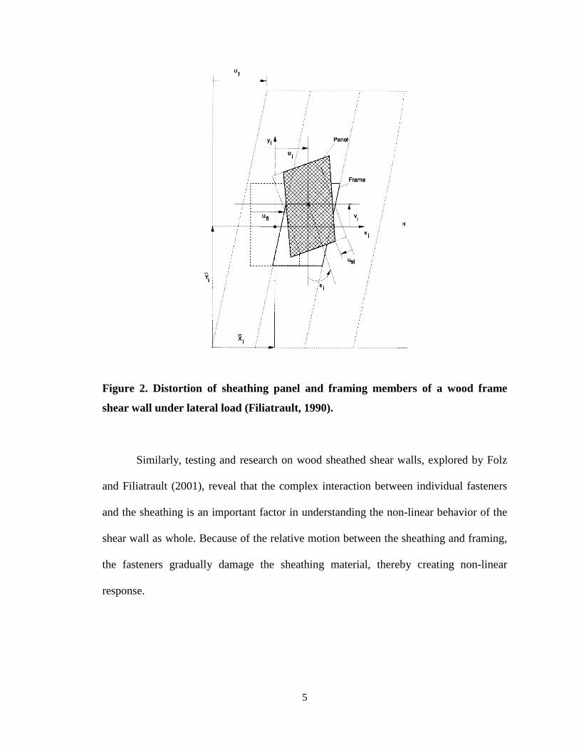
Figure 2. Distortion of sheathing panel and framing members of a wood frame
shear wall under lateral load (Filiatrault, 1990).
Similarly, testing and research on wood sheathed shear walls, explored by Folz
and Filiatrault (2001), reveal that the complex interaction between individual fasteners
and the sheathing is an important factor in understanding the non-linear behavior of the
shear wall as whole. Because of the relative motion between the sheathing and framing,
the fasteners gradually damage the sheathing material, thereby creating non-linear
response.
5
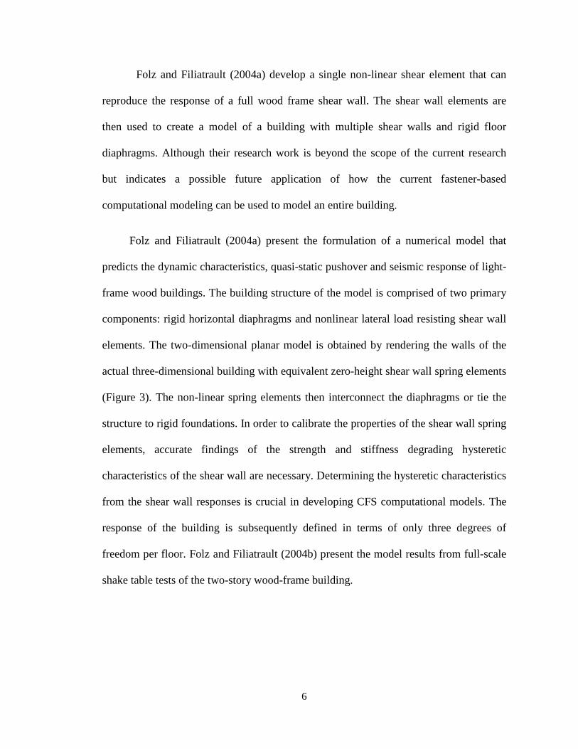
Folz and Filiatrault (2004a) develop a single non-linear shear element that can
reproduce the response of a full wood frame shear wall. The shear wall elements are
then used to create a model of a building with multiple shear walls and rigid floor
diaphragms. Although their research work is beyond the scope of the current research
but indicates a possible future application of how the current fastener-based
computational modeling can be used to model an entire building.
Folz and Filiatrault (2004a) present the formulation of a numerical model that
predicts the dynamic characteristics, quasi-static pushover and seismic response of light-
frame wood buildings. The building structure of the model is comprised of two primary
components: rigid horizontal diaphragms and nonlinear lateral load resisting shear wall
elements. The two-dimensional planar model is obtained by rendering the walls of the
actual three-dimensional building with equivalent zero-height shear wall spring elements
(Figure 3). The non-linear spring elements then interconnect the diaphragms or tie the
structure to rigid foundations. In order to calibrate the properties of the shear wall spring
elements, accurate findings of the strength and stiffness degrading hysteretic
characteristics of the shear wall are necessary. Determining the hysteretic characteristics
from the shear wall responses is crucial in developing CFS computational models. The
response of the building is subsequently defined in terms of only three degrees of
freedom per floor. Folz and Filiatrault (2004b) present the model results from full-scale
shake table tests of the two-story wood-frame building.
6
(a)
(b)
Figure 3. (a) Three-dimensional model of single-story wood frame structure; (b)
Two-dimensional planar model of the same single-story wood frame structure
(Filiatrault, 2004).
7
2.2 Cold-Formed Steel Framed Shear walls
Xu and Martinez (2006) presents an analytical method that employs an iterative
procedure to evaluate the ultimate lateral strength and displacement of a cold-formed
steel shear wall with sheathing. The method takes into consideration the effects of
material property, thickness and geometry of sheathing and studs, spacing of studs, and
geometric arrangement of fasteners and framing members. The paper incorporates test
results derived from various fastener configurations from full-scale shear walls in order
to calibrate complex spring elements. Compared to this approach, our computational
approach allows us to investigate many more possible shear wall configurations and thus
to understand much more complex nature of the behavior of the shear walls without
modeling an entire building. In scenarios where experimental data is not readily
available for simple shear wall models, the analytical approach of Xu and Martinez
(2006) can provide quick practical estimates.
Celik and Engleder (2010) develop a semi-analytical model to calculate the shear
strength of cold-formed steel framed shear walls. The concept of the analytical model
was grounded on the understanding that the resulting shear resistance of the sheathed
wall can be calculated as the sum of individual fastener resistances. The physical tests
were based on several full-scale shear wall assemblies and shear load performance of
individual fasteners which connect plywood to cold-formed steel members. The tests
observed plywood pull-over failure at the bottom corners. Similar behavior is observed
in this thesis using the fastener-based computational analysis approach. Employing
8

statistical methods such as least square fitting, the physical testing results were
subsequently incorporated into the analytical model.
Fiorino, et al. (2006) proposes an analytical approach to predict the non-linear
shear vs. top wall displacement relationship of sheathed cold-formed shear walls under
nonlinear earthquake excitation. The research’s method relies on the available screw
connection test results. The analytical results, when compared to experiments, reveal
that the prediction of wall deflection is not as accurate as the strength prediction. In
addition, since the analytical method is based on limited experimental data on
connections and walls, the outcomes from proposed approach can only be considered as
preliminary results for actual implementation.
Fülöp and Dubina (2004) conducted a full-scale shear wall test on different wall
panels and parameters that influence the earthquake behavior of the light thin-walled
load bearing structures. From the paper’s experimental results, the wall panels display
significant shear-resistance in terms of rigidity and load bearing capacity to effectively
resist lateral loads. Moreover, hysteretic behavior is characterized by significant
pinching that reduces energy dissipation. The experiments also reveal that failure starts
at the bottom track in the anchor bolt region. Thus, the authors conclude that the strength
of the corner detail is critical since it can subsequently have effects on the initial rigidity
of the wall system. This loss of rigidity, in turn, can cause large sway and premature
failure of the panel. These findings can be applicable for the modeling of the anchors to
the bottom track in our research in order to avoid premature failure of the panel wall.
9
Fiorino, et al. (2012) presents the results of an extensive parametric non-linear
dynamic analysis carried out on one story buildings with sheathed cold-formed steel
structural systems. The research considers wall configurations and investigates
parameters such as sheathing panel, wall geometry, external screw spacing, seismic
weight and soil type. The analysis is performed using incremental dynamic analysis
(IDA) by applying an ad hoc model of the hysteretic response of the shear walls. This
IDA approach to studying the shear walls hysteresis is one of the main methods
employed in examining the sheathed cold-formed steel structure systems. Similar to our
research, this paper is based on the premise that the seismic behavior of shear walls is
strongly influenced by the sheathing-to-frame connections response, which is
characterized by non-linear and hysteretic pinching response.
The purpose of the research conducted by Della Corte et al. (2006) was to
investigate whether sheathed cold-formed steel structures can survive more violent
earthquakes which exceed the design intensity. The researchers claim that cold-formed
structures, if adequately designed, could be less vulnerable to seismic damage than other
ordinary structures. According to modern design standards, design basis earthquakes are
typically defined as earthquakes with a 10% probability of being exceeded in 50 years.
The numerical modeling of cold-formed shear walls takes into account two major
characteristics of the sheathed walls: strong nonlinearity of lateral load-displacement
relationship, and strong pinching of hysteresis loops. The conclusion from the research
was that sheathed steel stud walls can be designed to meet enhanced seismic standards in
low and medium seismic intensity zones. Based on the non-linear responses predicted
10
from our computational model, future application may include improving current
seismic design codes for CFS shear wall structures.
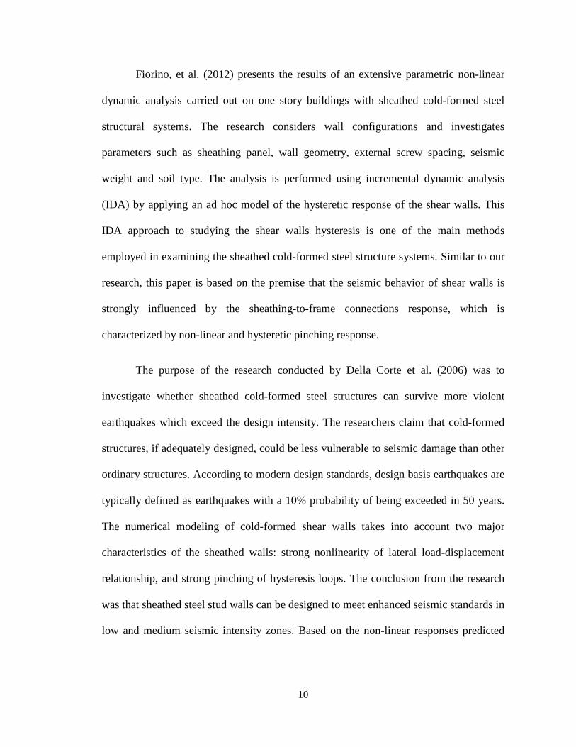
2.3 AISI S213 Code
American Iron and Steel Institute (AISI) classifies shear walls as either Type I
shear walls or Type II shear walls. For Type I shear walls, hold-downs are located at the
end of each shear wall “segment” whereas Type II only has two hold-downs, one at each
end of the wall (Figure 4). The present computational research employs Type I shear
walls.
Figure 4. Classification of shear walls: (a) Typical Type I Shear Wall, (b) Typical
Type II Shear Wall (AISI, 2007).
(a)
(b)
11

The strength and lateral deflection requirements for Type I shear walls in AISI
S213-07 were based on a series of investigations by Serrette (1996, 1997, 2002, 2003).
The available strength or factored resistance for a chosen assembly (in this case 7/16”
OSB sheathing wall) can be determined by using the nominal strength and dividing or
multiplying the appropriate safety factor (Ω) and resistance factor (φ), respectively
(Table 1).
Table 1. Nominal shear strength (Rn), safety factor (Ω) and resistance factor (φ) for
seismic loads for 7/16” OSB shear walls with given specifications
Assembly Description 7/16” OSB, one side
Max. Aspect Ratio (h/w) 2:1
Fastener Spacing at Panel Edges (inches) 6
Designation Thickness of Stud, Track and Blocking (mils) 54
Required Sheathing Screw Size 8
Required nominal Shear Strength (Rn) (pounds per foot) 940
Safety factor (Ω) (for ASD) 2.50
Resistance factor (φ) (for LRFD – seismic) 0.60
Resistance factor (φ) (for LSD – gypsum sheathed walls) 0.60
12

At the design strength, the lateral deflections of the computational shear wall
model are predicted. Equation C2.1-1 of AISI S213-07 provides calculation of the lateral
deflection of cold-formed steel light-framed shear walls (AISI, 2007):
vsheathingcs b
hvGt
vhbAE
vh δβ
ωωωωρ
ωωδ +
++=
2
4324/5
121
38 Eq (1)
where,
AC = gross cross-sectional area of chord member (in2)
b = width of the shear wall (ft.)
Es = modulus of elasticity of steel (= 29,500,000 psi)
G = shear modulus of sheathing material (psi)
h = wall height (ft.)
s = maximum fastener spacing at panel edges (in)
tsheathing = nominal panel thickness (in)
v = shear demand (V/b) (lb. per linear foot)
V = total lateral load applied to the shear wall (lb.)
β = 660 (for OSB)
δ = calculated deflection (in)
13
δv = vertical deformation of anchorage/ attachment details (in)
ρ = 1.05 for OSB
ω1 = s/6
ω2 = 0.033/tstud (tstud = framing designation thickness in inches)
ω3 = bh /5.0
ω4 = 1 (for wood structural panels)
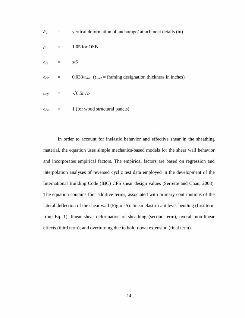
In order to account for inelastic behavior and effective shear in the sheathing
material, the equation uses simple mechanics-based models for the shear wall behavior
and incorporates empirical factors. The empirical factors are based on regression and
interpolation analyses of reversed cyclic test data employed in the development of the
International Building Code (IBC) CFS shear design values (Serrette and Chau, 2003).
The equation contains four additive terms, associated with primary contributions of the
lateral deflection of the shear wall (Figure 5): linear elastic cantilever bending (first term
from Eq. 1), linear shear deformation of sheathing (second term), overall non-linear
effects (third term), and overturning due to hold-down extension (final term).
14
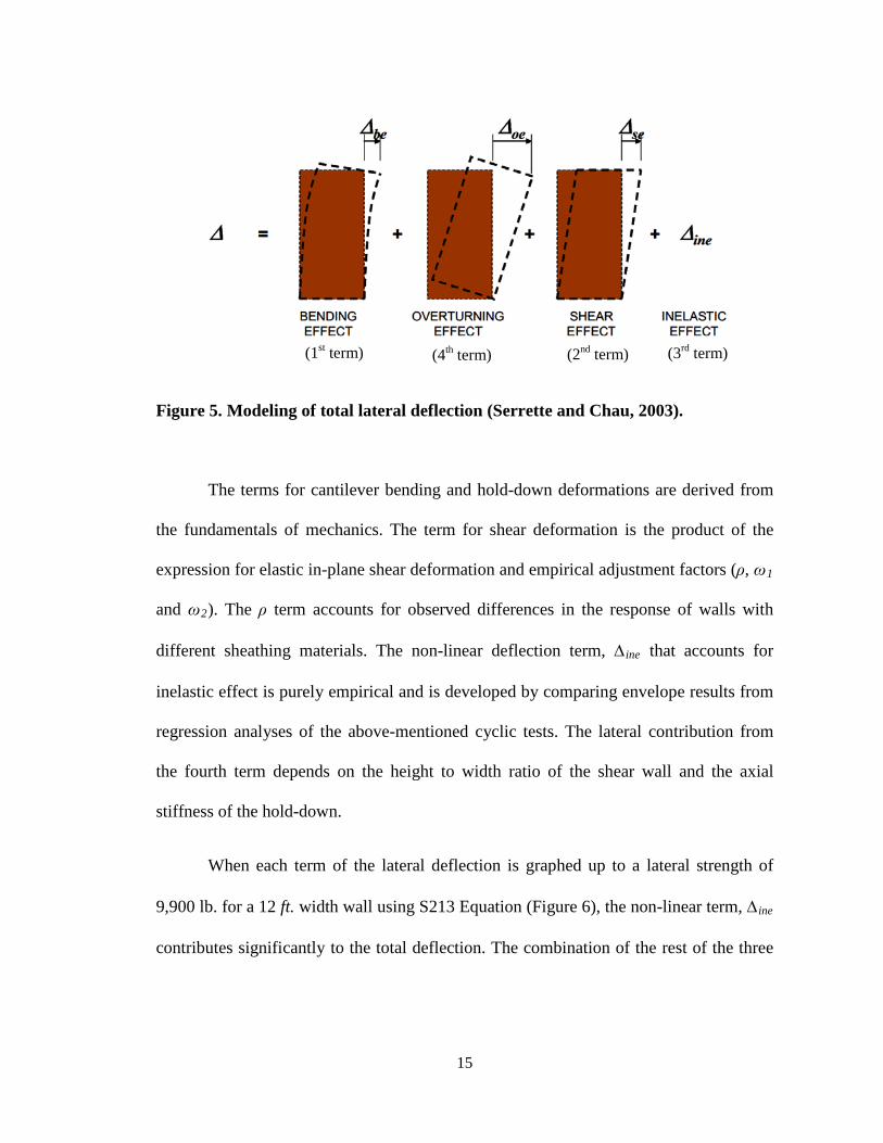
Figure 5. Modeling of total lateral deflection (Serrette and Chau, 2003).
The terms for cantilever bending and hold-down deformations are derived from
the fundamentals of mechanics. The term for shear deformation is the product of the
expression for elastic in-plane shear deformation and empirical adjustment factors (ρ, ω1
and ω2). The ρ term accounts for observed differences in the response of walls with
different sheathing materials. The non-linear deflection term, ∆ine that accounts for
inelastic effect is purely empirical and is developed by comparing envelope results from
regression analyses of the above-mentioned cyclic tests. The lateral contribution from
the fourth term depends on the height to width ratio of the shear wall and the axial
stiffness of the hold-down.
When each term of the lateral deflection is graphed up to a lateral strength of
9,900 lb. for a 12 ft. width wall using S213 Equation (Figure 6), the non-linear term, ∆ine
contributes significantly to the total deflection. The combination of the rest of the three
(1st term) (2nd term) (3rd term) (4th term)
15

terms, which can be mainly derived from mechanics, contributes less than 50% of the
total deflection. Since ∆ ine is a purely empirical term, little is known about what this
term actually entails. The fastener-based computational approach in this research seeks
to measure and explain this non-linear response and provide a better tool for its
prediction.
Figure 6. The effects of various deflection terms up to lateral strength (9900 lb.)
for a 12 ft. width wall based on Eq. C2.1-1 of AISI 213-07.
0 0.1 0.2 0.3 0.4 0.5 0.6 0.7 0.80
1000
2000
3000
4000
5000
6000
7000
8000
9000
10000
disp, in
forc
e, lb
cantileversheathingnon-lnearhold-downTotal
16
CHAPTER 3
3 DEVELOPMENT OF THE COMPUTATION MODEL
This research employs the OpenSees (Open System for Earthquake Engineering
Simulation) structural analysis software in order to create a fastener-based
computational model of CFS shear walls with sheathing. OpenSees is an object-oriented,
open source software framework that can create parallel finite element computer
applications for simulating the performance of structural and geotechnical systems
subjected to earthquakes (McKenna et al., 2011). Because it is a general purpose non-
linear dynamic analysis software, OpenSees permits modeling flexibility and has the
capability to incorporate multiple shear walls or a full building. While OpenSees is
employed to perform finite element analysis to obtain the seismic response data,
MATLAB is used to define the physical configurations of the shear wall models and
post-process the results.
3.1 Physical Testing of Shear Walls
Full-scale CFS shear walls specifically designed for a two-story ledger-framed
building underwent monotonic and cyclic tests in a structural lab at University of North
Texas and details of the tests can be found in Liu et al. (2012). The physical tests
examined the effects of geometry (varying widths of 4 ft. and 8 ft.), sheathing types
(OSB and gypsum), location of sheathing seam(s), and, presence of the framing ledger
17
on the nonlinear response. The general construction of the shear walls are detailed in
Figure 7 and the key features considered in the computational model are boxed in red.
Figure 7. Test setup and specimen details (Liu et al., 2012).
The basic geometries of 4 ft. x 9 ft. or 8 ft. x 9 ft. walls, framed with vertical studs,
are spaced 24 inches apart. The vertical studs were connected to the horizontal tracks
with No. 10 flathead screws. The exterior or chord studs are back-to-back double studs
and the interior or fixed studs are single studs. The studs and tracks are 600S162-54 and
600T150-54, respectively with both having yield strength of 50 ksi. The cold-formed
(a) front view (b) back view
Field Stud
Chord Stud
Bottom track
18

steel has a modulus of elasticity of 29,500 ksi and a shear modulus of 11,200 ksi. The
ledger is a 1200T200-097 section with yield strength of 50 ksi, and is attached to the top
1 ft. of the interior face of the CFS wall using No. 10 flathead screws. The following
table (Table 2) shows the section properties of studs, tracks and ledgers used in the
physical tests and computational models.
Table 2. Section properties of CFS studs, tracks and ledger
Properties Double stud Single stud Top track Bottom track Ledger
(2 x 600S162-54) (600S162-54) (600T150-54) (600T150-54) (1200T200-097)
Area (in.2) 2×0.556 0.556 0.509 0.509 1.63
Moment of inertia (strong axis) (in.4)
2×2.86 2.86 2.61 2.61 29.8
Moment of inertia (weak axis) (in.4)
1.0244 0.329 0.0907 0.0907 0.41
Torsional inertia (in.4) 2×5.94×10-4 5.94×10⁻⁴ 5.43×10⁻⁴ 5.43×10⁻⁴ 5.60×10⁻³
The physical tests used No. 8 flathead screws (1-15/16 in. long) to fasten the
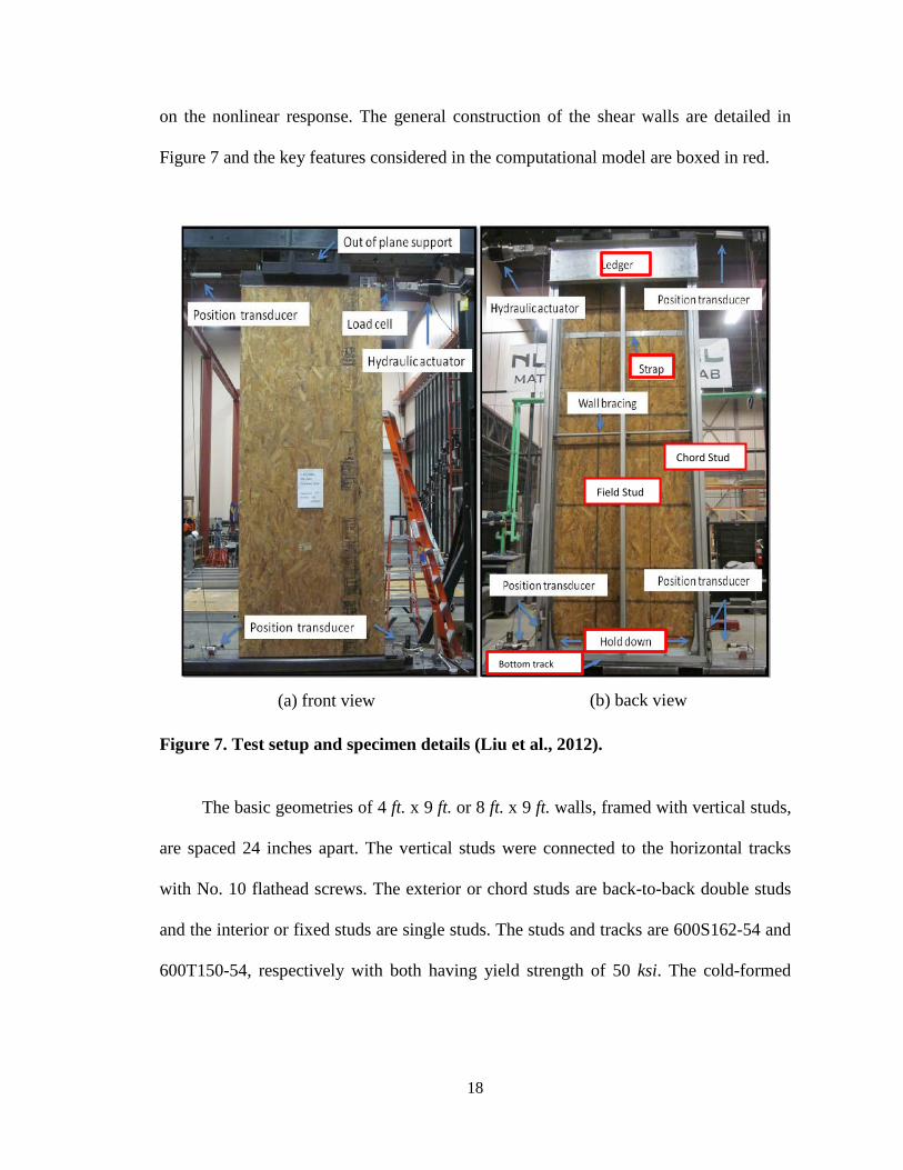
7/16 in. thick orientated strand board (OSB) sheathing to the studs and tracks. The OSB
type was 24/16, exposure 1 rated. On the perimeter of the sheathing, the screws were
spaced at 6 in., and along the interior studs, the screws were spaced at 12 in. (Figure 8).
CFS construction contains horizontal and vertical seams in the OSB sheathing because
the sheathing is commonly manufactured in 4 ft. x 8 ft. sheets. Vertical seams are
supported at interior stud location at every 4 ft. width. Horizontal seams are bridged with
a 1.5 in. wide 54 mil steel seam strap.
19
Figure 8. Typical CFS shear wall configuration (Buonopane et al., 2014).
Simpson StrongTie® S/HDU6 hold-downs with No.14 HWT self-drilling screws
were installed at the exterior chord studs. The hold-downs were connected to the steel
base using 5/8 in. diameter 2.5 in. long ASTM 325 anchor bolts. In addition, the bottom
track of the shear walls were bolted to the steel testing frame with 5/8 in. anchor bolts at
24 in. on-center along the wall with standard washers and nuts. In typical CFS
construction, the shear anchors would consist of low-velocity fasteners anchored into the
foundation material. Four bolts were used for 4 ft. x 9 ft. shear walls and six bolts for 8
ft. x 9 ft. shear walls (Figure 9).
20

Figure 9. Hold-down and anchor placements along frame base (top view) for: (a) 4
ft. and (b) 8 ft. wide wall (Liu et al., 2012).
Monotonic and cyclic tests were performed in displacement control, following
ASTM E564 (2006). According to the test results, specimens generally failed at
perimeter and corner sheathing-to-stud fastener locations. The most common failure
modes were a pull-through or bearing failure. Figure 10 illustrates all observed fastener
failure modes and Figure 11 displays the force-displacement response of a typical shear
wall, along with key response results.
21
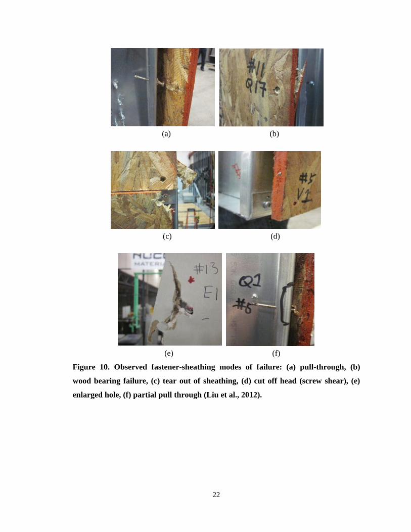
Figure 10. Observed fastener-sheathing modes of failure: (a) pull-through, (b)
wood bearing failure, (c) tear out of sheathing, (d) cut off head (screw shear), (e)
enlarged hole, (f) partial pull through (Liu et al., 2012).
(a) (b)
(c) (d)
(e) (f)
22
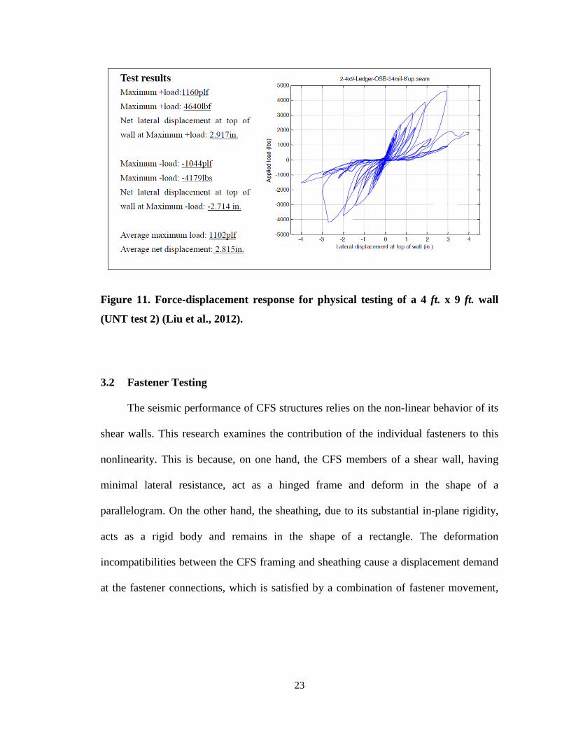
Figure 11. Force-displacement response for physical testing of a 4 ft. x 9 ft. wall
(UNT test 2) (Liu et al., 2012).
3.2 Fastener Testing
The seismic performance of CFS structures relies on the non-linear behavior of its
shear walls. This research examines the contribution of the individual fasteners to this
nonlinearity. This is because, on one hand, the CFS members of a shear wall, having
minimal lateral resistance, act as a hinged frame and deform in the shape of a
parallelogram. On the other hand, the sheathing, due to its substantial in-plane rigidity,
acts as a rigid body and remains in the shape of a rectangle. The deformation
incompatibilities between the CFS framing and sheathing cause a displacement demand
at the fastener connections, which is satisfied by a combination of fastener movement,
23

fastener deformation, and localized deformation and damage to the sheathing
surrounding the individual fastener (Figure 12).
Figure 12. Display of fastener displacement demand: (a) Initial Configuration; (b)
Deformed Configuration; (c) Deformed Cross-sectional Details (Buonopane et al.,
2014).
The force-displacement behavior of the fastener connections is found to be
greatly non-linear, displaying the characteristics of hysteresis, degradation and pinching
(Section 2.2). The local behavior of each individual fastener collectively creates the non-
linear force-deflection response of the CFS shear wall as a whole (Figure 12). There are
several approaches to capture the non-linear behavior of the shear walls in
computational models. One approach would be to calibrate complex shell or spring
elements using test results from full-scale shear walls (Fülöp and Dubina, 2004).
However, estimating non-linear properties is difficult if there are no companion test
24
results. The method employed in this research is to model the location and behavior of
each fastener, with individual fastner behavior defined based on experimental results.
The approach allows simplifying assumptions such as semi-rigid and flexible CFS
members and the option to include hold-down flexibility. Using results from a series of
experiments conducted at Johns Hopkins University (JHU), the researchers there
characterized and normalized the force-displacement behavior occurring at individual
fasteners.
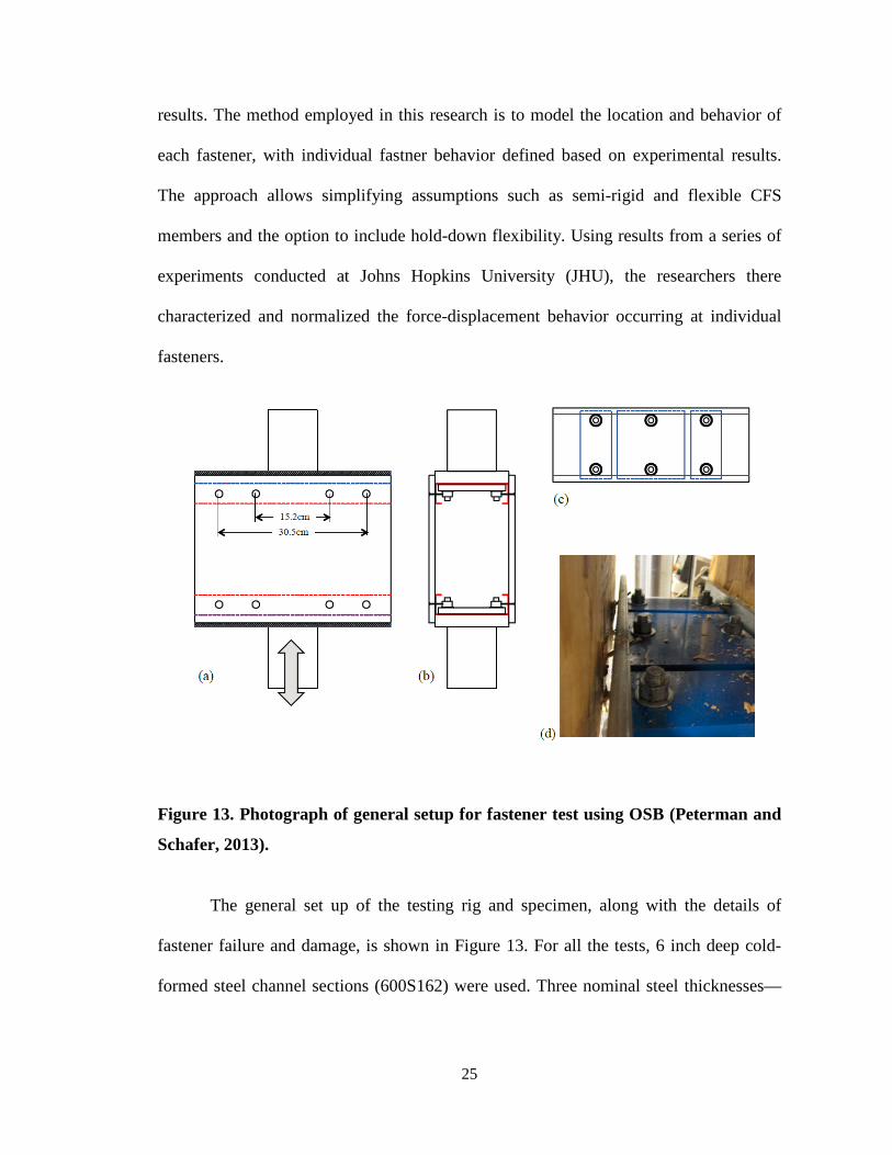
Figure 13. Photograph of general setup for fastener test using OSB (Peterman and
Schafer, 2013).
The general set up of the testing rig and specimen, along with the details of
fastener failure and damage, is shown in Figure 13. For all the tests, 6 inch deep cold-
formed steel channel sections (600S162) were used. Three nominal steel thicknesses—
25
33, 54, and 97 mil—were tested. Two fastener spacings—6 inches and 12 inches to
simulate typical spacings used in chord and field studs, respectively—were also tested.
From monotonic tests, it was determined that the fastener spacings of either 6 or 12
inches do not significantly affect the strength of the connection between CFS and
sheathing. In addition, the fastener stiffness <GIVE VALUE> from the monotonic tests
is used as the fastener stiffness for the linear analysis models in OpenSees.
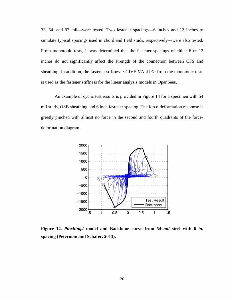
An example of cyclic test results is provided in Figure 14 for a specimen with 54
mil studs, OSB sheathing and 6 inch fastener spacing. The force-deformation response is
greatly pinched with almost no force in the second and fourth quadrants of the force-
deformation diagram.
Figure 14. Pinching4 model and Backbone curve from 54 mil steel with 6 in.
spacing (Peterman and Schafer, 2013).
26

Hysteretic characterization of the stud-fastener-sheathing performance was
accomplished by using the Pinching4 material model, as implemented in OpenSees
(Lowes, et al., 2004). As depicted in Figure 15, Pinching4 parameters include four
positive and four negative points that define the loading or backbone curve, and six
additional parameters that define the unloading and re-loading behavior of the material.
Figure 15. Pinching4 hysteresis parameters (Lowes, et al., 2004).
Using the Pinching4 model, the behavioral response of each individual fastener can be
approximated computationally. An example of the fitted Pinching4 model imposed on
the actual test data is provided in Figure 16.
27
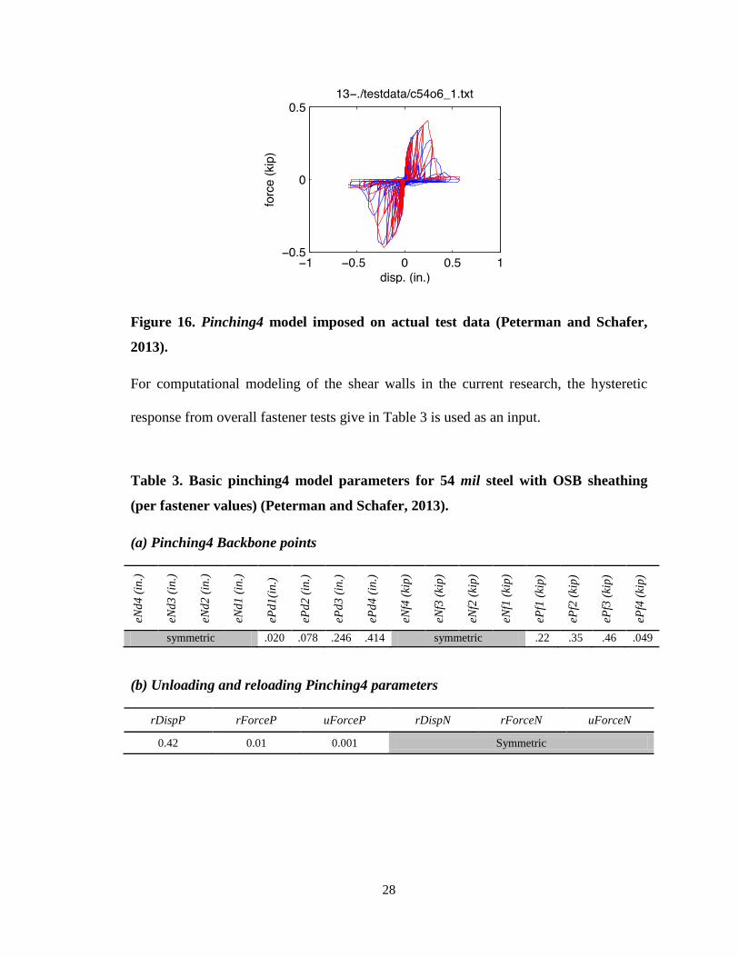
Figure 16. Pinching4 model imposed on actual test data (Peterman and Schafer,
2013).
For computational modeling of the shear walls in the current research, the hysteretic
response from overall fastener tests give in Table 3 is used as an input.
Table 3. Basic pinching4 model parameters for 54 mil steel with OSB sheathing
(per fastener values) (Peterman and Schafer, 2013).
(a) Pinching4 Backbone points
eNd4
(in.
)
eNd3
(in.
)
eNd2
(in.
)
eNd1
(in.
)
ePd1
(in.)
ePd2
(in.
)
ePd3
(in.
)
ePd4
(in.
)
eNf4
(kip
)
eNf3
(kip
)
eNf2
(kip
)
eNf1
(kip
)
ePf1
(kip
)
ePf2
(kip
)
ePf3
(kip
)
ePf4
(kip
) symmetric .020 .078 .246 .414 symmetric .22 .35 .46 .049
(b) Unloading and reloading Pinching4 parameters
rDispP rForceP uForceP rDispN rForceN uForceN
0.42 0.01 0.001 Symmetric
28
3.3 Development of the Computational Model
3.3.1 Test matrix
The computational modeling for this research combines the non-linear force-
deformation relationship for individual fasteners with the overall geometry and
structural properties of the sheathing and the CFS framing. In addition to the overall
wall geometry and fastenter layout, the analyses focus on examining four specific
modeling aspects: hold-downs, shear anchors, vertical seams and ledger track. Table 4
summarizes different model variations.
29

Table 4. Summary of OpenSees model variations with their respective initial linear
stiffness and displacement at 1000 lb. lateral force
Analysis
Name
Width
(ft.)
Model Features
hold
down
shear
anchors
vertical
seam
ledger as
diaphragm
L4_1 4 pinned none n/a no
L4_2 4 elastic none n/a no
L4_3 4 elastic pinned n/a no
L4_4 4 elastic pinned n/a yes
L4_5 4 elastic none n/a yes
L8_1 8 pinned none 1 no
L8_2d 8 elastic none 1 no
L8_3 8 elastic pinned 1 no
L8_4 8 elastic pinned 1 yes
L8_5d 8 elastic none 1 yes
L8_2s 8 elastic none no no
L8_5s 8 elastic none no yes
L12_1 12 pinned none 2 no
L12_2t 12 elastic none 2 no
L12_3 12 elastic pinned 2 no
L12_4 12 elastic pinned 2 yes
L12_5t 12 elastic none 2 yes
L12_2s 12 elastic none no no
L12_5s 12 elastic none no yes
30
3.3.2 Geometry and Nodes
The OpenSees models represent three basic shear wall sizes: 4 ft. x 9 ft., 8 ft. x 9
ft., and 12 ft. x 9 ft. The physical configuration of a 4 ft. x 9 ft. shear wall is illustrated in
Figure 17 and the node locations of the computation model are defined in Figure 18. The
results of the computational models are compared to several shear wall tests performed
at UNT (Liu et al., 2012).
Figure 17. Geometry of 4 ft. x 9 ft. Physical CFS-OSB Shear Wall (Liu et al., 2012).
(a) front view (b) back view
31

Figure 18. Nodes of a 4 ft. x 9 ft. OpenSees CFS-OSB Shear Wall Model.
3.3.3 CFS Studs and Tracks
The CFS tracks and studs were modeled using displacement-based beam
elements (dispBeamColumn in OpenSees) with section properties given in Table 2 of
Section 3.1. The steel framing members were subdivided with a node at each fastener
location.
32
3.3.4 OSB Sheathing Panels
The OSB sheathing panels are modeled as rigid diaphragms, which include slave
nodes at every fastener location and a master node at the center of the panel. The model
does not incorporate the panel’s shear stiffness.
3.3.5 Fastener Elements
Two coincident nodes were defined at each fastener location: one on the CFS
frame members and another on the sheathing diaphragm. The fastener elements are one-
dimensional, zero-length, radially symmetric elements (CoupledZeroLength). The
uniaxial material properties assigned to the fastener elements are based on the results of
physical testing of fasteners as described in Section 3.2. The radial stiffness of the
fasteners is 12,205 lb./in (Peterman and Schafer, 2013). for linear analyses. For non-
linear analyses, the fastener material is defined as a Pinching4 material, which includes a
multi-linear backbone curve and pinching (see Table 3 from Section 3.2.).
3.3.6 Ledger Track
The ledger track is modeled by creating a rigid diaphragm having the rectangular
area equal to that of the web of the track. Since the ledger is directly connected to the
studs in the physical model, the diaphragm in the computational model is also directly
connected to the CFS frame nodes. As in the sheathing, the master node is again defined
at the center of the rectangular area of the ledger. Although this does not account for the
33

deformation of the ledger track, the modeling is simpler than using a series of beam-
column elements and rigid offsets to represent the ledger.
3.3.7 Stud-to-track Connections
The connections between vertical studs and top and bottom tracks were modeled
as semi-rigid connections in rotation only. The nodes were connected by a rotational
linear elastic spring and rigidly connected in translational degrees of freedom. Based on
the measured lateral stiffness of the 4 ft. and 8 ft. bare CFS frames, the spring’s
rotational stiffness was estimated to be 100,000 in-lb./rad. This estimate was obtained
by first analytically deriving the relationship between the stiffness of the CFS frame
members and the rotational stiffness of stud-to-track connectors, and back-calculating
the latter based on the measured stiffness of the UNT bare frame experiments (Liu et al.,
2012).
3.3.8 Horizontal and Vertical Seams
CFS construction contains horizontal and vertical seams in the OSB sheathing:
vertical seams are always supported by an interior stud and horizontal seams are bridged
with a steel seam strap. In the OpenSees models, cases having no vertical seams (i.e. a
single rigid diaphragm across the entire wall) and those having vertical seams spaced
every 4 ft. (i.e. multiple dipahraghms) were investigated. A single diaphragm with no
seams was the simpler computational model.
34
To models the shear walls with vertical seams, multiple rigid diaphragms, each
of which is 4 ft. wide by 9 ft. tall, are created in OpenSees—thus the 8 ft. wide walls
have two equal-width rigid diaphragms, and the 12 ft. walls have three. In the OpenSees
models, the rigid diaphragms are allowed to slide past one another without interference.
In actual construction the seam strap provide sufficient stiffness to prevent relative
motion of the panels across the horizontal seam, and the strength of the seam strap
sufficient to prevent its failure in typical applications. Preliminary study of models with
horizontal seams revealed that additional modeling of steel straps would be necessary to
restrain the large displacements which occur across a horizontal seam with no strap.
Therefore, the computational models do not include the horizontal seam straps and
instead use a single diaphragm across the vertical 9 ft. height.
3.3.9 Support Conditions
The physical tests include the hold-downs at the exterior chord studs, the bottom
track includes additional nodes, offset 1.4375 in. from the centerline of the double stud
to the position of the hold-down anchor bolt.
In the lateral translational direction, the hold-downs were modeled as fixed. In
the rotational direction, the hold-downs were pinned. In the axial direction they were
modeled as infinitely stiff (rigid) or by a uniaxial spring element. In the latter model, the
tension stiffness of the hold-down was 56.7 kips/in. (Leng et al., 2013) and the
compression stiffness was assigned a value of 1000 times greater than the tension
stiffness in order to approximate bearing on a rigid foundation. The modeling of hold-
35
downs as a uniaxial spring element allows for non-linear analysis and is suitable for
future cyclic tests. Shear anchors are not included in every OpenSees model but when
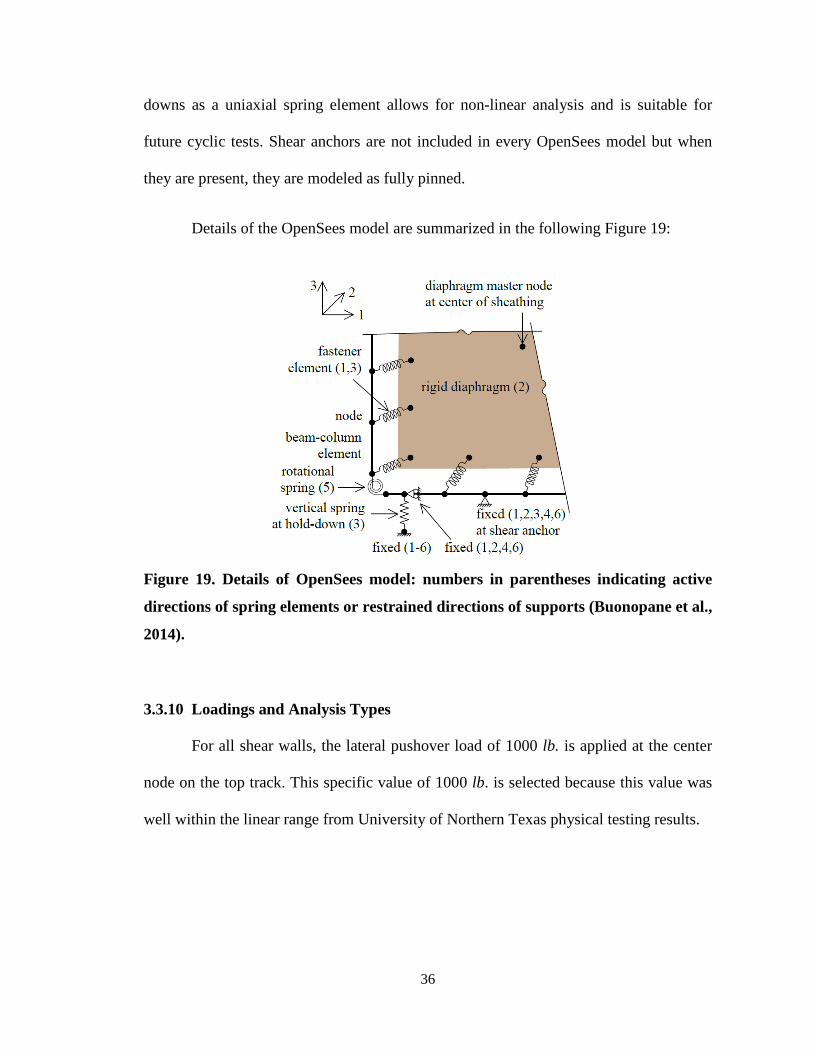
they are present, they are modeled as fully pinned.
Details of the OpenSees model are summarized in the following Figure 19:
Figure 19. Details of OpenSees model: numbers in parentheses indicating active
directions of spring elements or restrained directions of supports (Buonopane et al.,
2014).
3.3.10 Loadings and Analysis Types
For all shear walls, the lateral pushover load of 1000 lb. is applied at the center
node on the top track. This specific value of 1000 lb. is selected because this value was
well within the linear range from University of Northern Texas physical testing results.
36

CHAPTER 4
4 RESULTS AND DISCUSSION
4.1 Linear Result Validations and Disucssion
The computational results are validated using three main methods:
(1) by drawing free-body diagrams of the shear wall panel and analyzing
equilibrium at the support reactions,
(2) by employing equation C2.1-1 of AISI S213-07 and comparing the lateral
deflections, and,
(3) by comparing computational results to experimental from University of
Northern Texas.
In Table 5, the linear stiffnesses and displacements due to a 1000 lb. lateral force
from all OpenSees models are shown.
37

Table 5. Stiffness and displacement from OpenSees linear analyses with applied
1000 lb. lateral force
Analysis Name
Stiffness (lb./in.)
Displacement (in.)
Comparison Test [#]
L4_1 14292 0.070 4
L4_2 5357 0.187 4
L4_3 9774 0.102 4
L4_4 11922 0.084 2
L4_5 5812 0.172 2
L8_1 32219 0.031 14
L8_2d 17714 0.057 14
L8_3 27462 0.036 14
L8_4 37188 0.027 12
L8_5d 20551 0.049 12
L8_2s 22214 0.045 14
L8_5s 24485 0.041 12
L12_1 48358 0.021 n/a
L12_2t 31757 0.032 n/a
L12_3 44953 0.022 n/a
L12_4 64007 0.016 n/a
L12_5t 38637 0.026 n/a
L12_2s 45497 0.022 n/a
L12_5s 52730 0.019 n/a
38
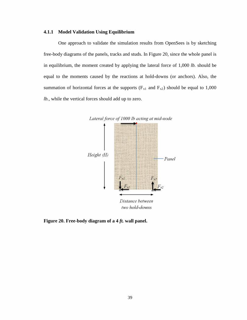
4.1.1 Model Validation Using Equilibrium
One approach to validate the simulation results from OpenSees is by sketching
free-body diagrams of the panels, tracks and studs. In Figure 20, since the whole panel is
in equilibrium, the moment created by applying the lateral force of 1,000 lb. should be
equal to the moments caused by the reactions at hold-downs (or anchors). Also, the
summation of horizontal forces at the supports (Fx1 and Fx2) should be equal to 1,000
lb., while the vertical forces should add up to zero.
Figure 20. Free-body diagram of a 4 ft. wall panel.
39

Sample Calculation
For example, in linear analysis L4_1, the reactions are Fx1 = 500 lb., Fx2 =
499.92 lb., Fy1= 2571 lb. and Fy2 = 2571 lb. Thus, the summation of all the vertical
reactions is equal to zero, and the sum of the horizontal reaction forces at the two hold-
downs are approximately equal to 1,000 lb. applied load. Since the distance between two
hold-downs is 42 in., the moment taken about the left hold-down due to Fy2 is 107,982
lb.-in. This is approximately equal to moment created by the 1000 lb. lateral load
(108,000 lb.-in). The small discrepancy between the two results is due to the nonlinear
modeling of hold-downs as a uniaxial spring element.
OpenSees analyses also provide visualization of the entire shear wall (Figure 21).
The blue and yellow panels represent OSB sheathing of the shear wall before and after the
lateral load is applied, respectively. The original position of the framing studs and tracks
are colored in red, and the displaced position in blue. Moreover, OpenSees can create
graphical diagrams for the internal forces (axial, shear, moment) in the framing members
as a result of force transfer at each individual fastener as shown in Figure 22a-f. At a
minimum, the graphical diagrams reveal and validate the fundatmental relationships
between axial, shear and moment diagrams.
40

Figure 21. Visualization of model L4_1 at 1000 lb. lateral force.
41

(b)
(a)
42

(c)
(d)
43
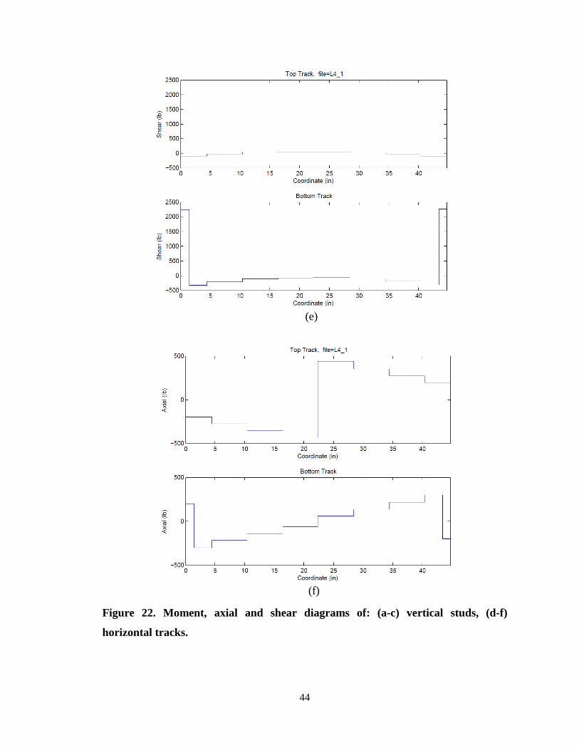
Figure 22. Moment, axial and shear diagrams of: (a-c) vertical studs, (d-f)
horizontal tracks.
(e)
(f)
44
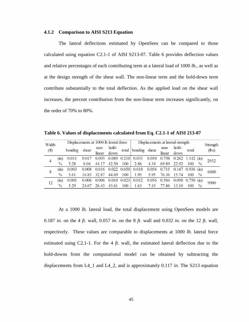
4.1.2 Comparison to AISI S213 Equation
The lateral deflections estimated by OpenSees can be compared to those
calculated using equation C2.1-1 of AISI S213-07. Table 6 provides deflection values
and relative percentages of each contributing term at a lateral load of 1000 lb., as well as
at the design strength of the shear wall. The non-linear term and the hold-down term
contribute substantially to the total deflection. As the applied load on the shear wall
increases, the percent contribution from the non-linear term increases significantly, on
the order of 70% to 80%.
Table 6. Values of displacements calculated from Eq. C2.1-1 of AISI 213-07
At a 1000 lb. lateral load, the total displacement using OpenSees models are
0.187 in. on the 4 ft. wall, 0.057 in. on the 8 ft. wall and 0.032 in. on the 12 ft. wall,
respectively. These values are comparable to displacements at 1000 lb. lateral force
estimated using C2.1-1. For the 4 ft. wall, the estimated lateral deflection due to the
hold-downs from the computational model can be obtained by subtracting the
displacements from L4_1 and L4_2, and is approximately 0.117 in. The S213 equation
45

predicts the lateral displacement to be 0.089 in. Similarly for the 8 ft. wall, the lateral
deflection prediction from the S213 equation is 0.022 in. and from OpenSees 0.026 in
(subtracting the lateral displacement of L8_1 from that of L8_2d). For the 12 ft. wall, the
S213 lateral deflection is 0.010 in. and OpenSees deflection is 0.011 in. (subtracting the
displacements from L12_1 and L12_2t). Thus, the two methods generally produce
favorably comparable displacement results. It is important to note that these OpenSees
models do not account for the sheathing shear flexibility. Therefore, the deflections from
the computational model could be slightly increased by including the shear term from
the S213 equation.
4.1.3 Comparison to Experimental Results
The linear analyses focus on examining the accuracy of four modeling features:
hold-downs, shear anchors, vertical seams and ledger track (Table 4). The initial
stiffnesses from OpenSees models are superimposed on the experimental results from
University of Northern Texas (Liu et al., 2012).
By comparing the available experimental (Liu et al., 2012) and computational
results of the 4 ft. and 8 ft. walls (L4_1 vs. L4_2 and L8_1 vs. L8_2d), it is observed that
modeling of hold-down requires tension flexibility (Figure 23).
46
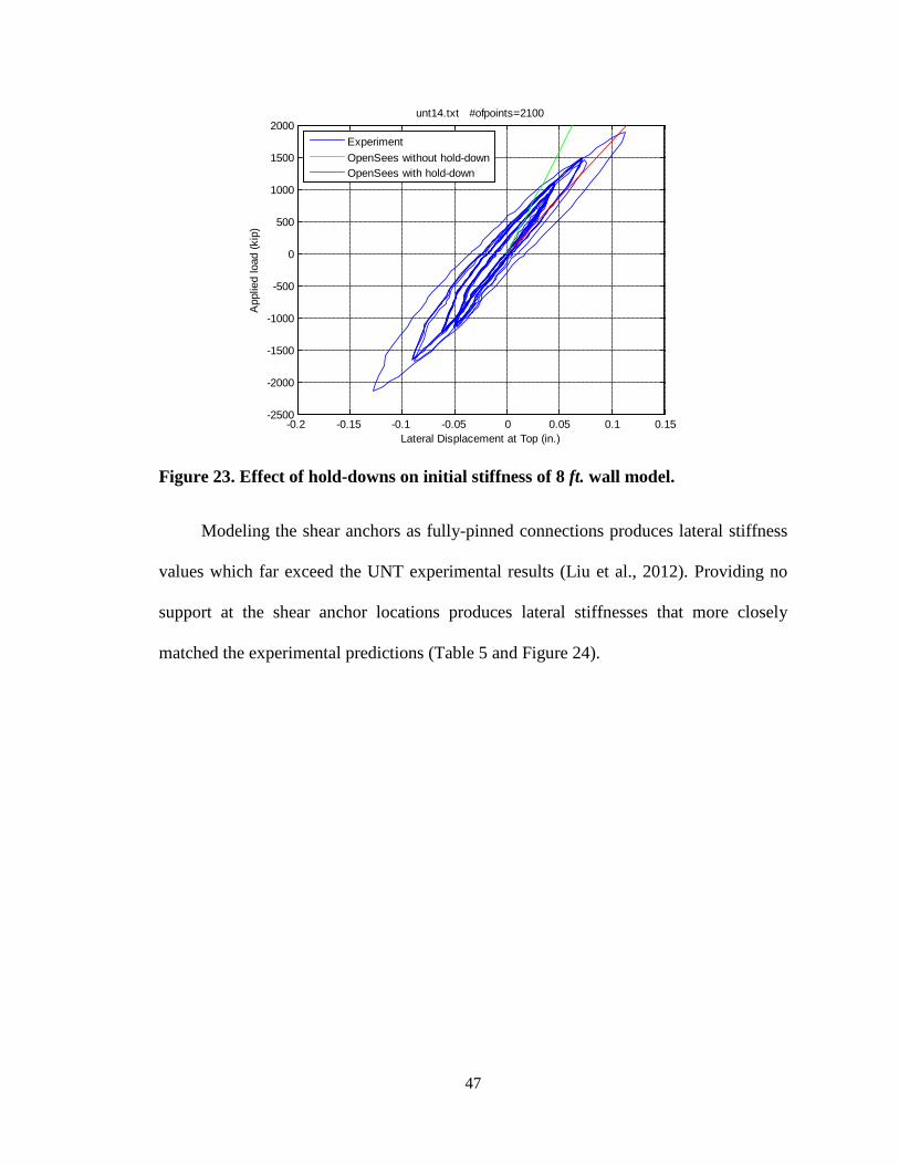
Figure 23. Effect of hold-downs on initial stiffness of 8 ft. wall model.
Modeling the shear anchors as fully-pinned connections produces lateral stiffness
values which far exceed the UNT experimental results (Liu et al., 2012). Providing no
support at the shear anchor locations produces lateral stiffnesses that more closely
matched the experimental predictions (Table 5 and Figure 24).
-0.2 -0.15 -0.1 -0.05 0 0.05 0.1 0.15-2500
-2000
-1500
-1000
-500
0
500
1000
1500
2000
Lateral Displacement at Top (in.)
App
lied
load
(kip
)
unt14.txt #ofpoints=2100
ExperimentOpenSees without hold-downOpenSees with hold-down
47
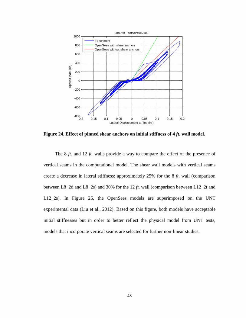
Figure 24. Effect of pinned shear anchors on initial stiffness of 4 ft. wall model.
The 8 ft. and 12 ft. walls provide a way to compare the effect of the presence of
vertical seams in the computational model. The shear wall models with vertical seams
create a decrease in lateral stiffness: approximately 25% for the 8 ft. wall (comparison
between L8_2d and L8_2s) and 30% for the 12 ft. wall (comparison between L12_2t and
L12_2s). In Figure 25, the OpenSees models are superimposed on the UNT
experimental data (Liu et al., 2012). Based on this figure, both models have acceptable
initial stiffnesses but in order to better reflect the physical model from UNT tests,
models that incorporate vertical seams are selected for further non-linear studies.
-0.2 -0.15 -0.1 -0.05 0 0.05 0.1 0.15 0.2-800
-600
-400
-200
0
200
400
600
800
1000
Lateral Displacement at Top (in.)
App
lied
load
(kip
)
unt4.txt #ofpoints=2100
ExperimentOpenSees with shear anchorsOpenSees without shear anchors
48
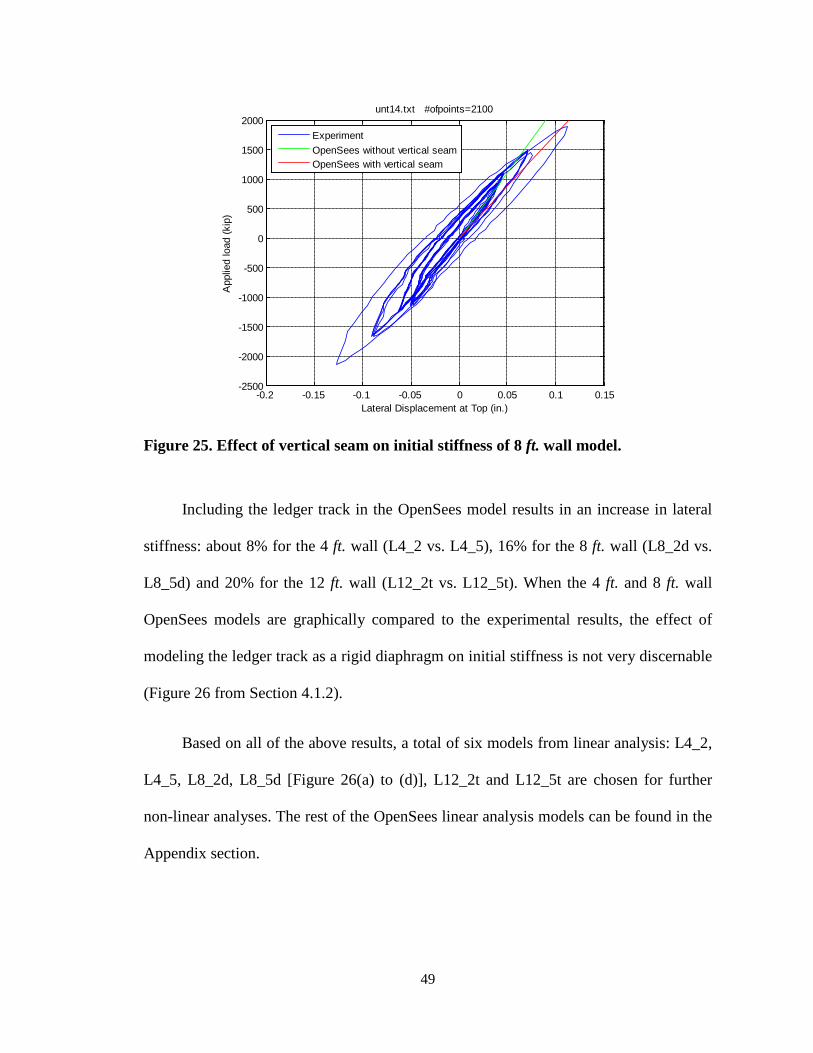
Figure 25. Effect of vertical seam on initial stiffness of 8 ft. wall model.
Including the ledger track in the OpenSees model results in an increase in lateral
stiffness: about 8% for the 4 ft. wall (L4_2 vs. L4_5), 16% for the 8 ft. wall (L8_2d vs.
L8_5d) and 20% for the 12 ft. wall (L12_2t vs. L12_5t). When the 4 ft. and 8 ft. wall
OpenSees models are graphically compared to the experimental results, the effect of
modeling the ledger track as a rigid diaphragm on initial stiffness is not very discernable
(Figure 26 from Section 4.1.2).
Based on all of the above results, a total of six models from linear analysis: L4_2,
L4_5, L8_2d, L8_5d [Figure 26(a) to (d)], L12_2t and L12_5t are chosen for further
non-linear analyses. The rest of the OpenSees linear analysis models can be found in the
Appendix section.
-0.2 -0.15 -0.1 -0.05 0 0.05 0.1 0.15-2500
-2000
-1500
-1000
-500
0
500
1000
1500
2000
Lateral Displacement at Top (in.)
App
lied
load
(kip
)
unt14.txt #ofpoints=2100
ExperimentOpenSees without vertical seamOpenSees with vertical seam
49

-0.1 -0.05 0 0.05 0.1 0.15 0.2 0.25-400
-200
0
200
400
600
800
1000
Lateral Displacement at Top (in.)
App
lied
load
(kip
)
unt4.txt L4_2 #ofpoints=1000
ExperimentOpenSees
-0.2 -0.15 -0.1 -0.05 0 0.05 0.1 0.15 0.2-1000
-800
-600
-400
-200
0
200
400
600
800
1000
Lateral Displacement at Top (in.)
App
lied
load
(kip
)
unt2.txt L4_5 #ofpoints=2100
ExperimentOpenSees
(a)
(b)
50

Figure 26. Chosen linear models with OpenSees initial stiffness graphs (red)
superimposed on the UNT experimental data (Liu et al., 2012) (blue) : (a) L4_2, (b)
L4_5, (c) L8_2d, (d) L8_5d.
-0.2 -0.15 -0.1 -0.05 0 0.05 0.1 0.15-2500
-2000
-1500
-1000
-500
0
500
1000
1500
2000
Lateral Displacement at Top (in.)
App
lied
load
(kip
)
unt14.txt L8_2d #ofpoints=2100
ExperimentOpenSees
-0.15 -0.1 -0.05 0 0.05 0.1 0.15 0.2-2000
-1500
-1000
-500
0
500
1000
1500
2000
2500
Lateral Displacement at Top (in.)
App
lied
load
(kip
)
unt12.txt L8_5d #ofpoints=2100
ExperimentOpenSees
(c)
(d)
51
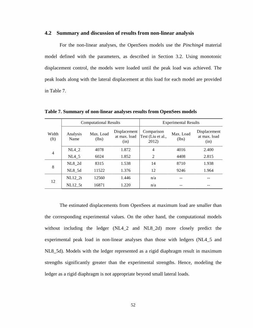
4.2 Summary and discussion of results from non-linear analysis
For the non-linear analyses, the OpenSees models use the Pinching4 material
model defined with the parameters, as described in Section 3.2. Using monotonic
displacement control, the models were loaded until the peak load was achieved. The
peak loads along with the lateral displacement at this load for each model are provided
in Table 7.
Table 7. Summary of non-linear analyses results from OpenSees models
The estimated displacements from OpenSees at maximum load are smaller than
the corresponding experimental values. On the other hand, the computational models
without including the ledger (NL4_2 and NL8_2d) more closely predict the
experimental peak load in non-linear analyses than those with ledgers (NL4_5 and
NL8_5d). Models with the ledger represented as a rigid diaphragm result in maximum
strengths significantly greater than the experimental strengths. Hence, modeling the
ledger as a rigid diaphragm is not appropriate beyond small lateral loads.
Computational Results Experimental Results
Width (ft)
Analysis Name
Max. Load (lbs)
Displacement at max. load
(in)
Comparison Test (Liu et al.,
2012)
Max. Load (lbs)
Displacement at max. load
(in)
4 NL4_2 4078 1.872 4 4016 2.400 NL4_5 6024 1.852 2 4408 2.815
8 NL8_2d 8315 1.538 14 8710 1.938 NL8_5d 11522 1.376 12 9246 1.964
12 NL12_2t 12560 1.446 n/a -- --
NL12_5t 16871 1.220 n/a -- --
52
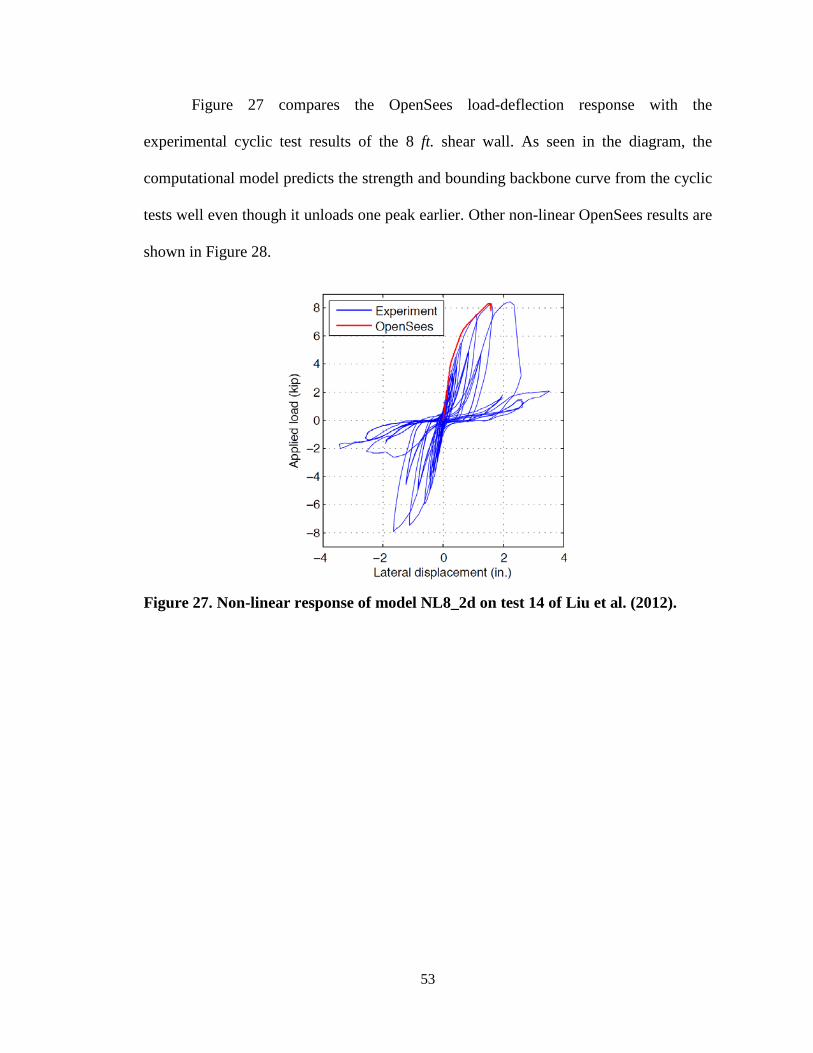
Figure 27 compares the OpenSees load-deflection response with the
experimental cyclic test results of the 8 ft. shear wall. As seen in the diagram, the
computational model predicts the strength and bounding backbone curve from the cyclic
tests well even though it unloads one peak earlier. Other non-linear OpenSees results are
shown in Figure 28.
Figure 27. Non-linear response of model NL8_2d on test 14 of Liu et al. (2012).
53

(a)
(b)
54

Figure 28. OpenSees non-linear responses: (a) model NL4_2 superimposed on UNT
test 4 of Peterman and Schafer (2013), (b) model NL4_5 superimposed on UNT test
2 of Peterman and Schafer (2013), (c) model NL8_5d superimposed on UNT test 12
of Peterman and Schafer (2013), (d) models NL12_2t and NL12_5t (no
experimental data available).
(c)
(d)
55

Modeling the individual fasteners permits a more detailed examination of the
interaction forces between the fasteners, the framing members and the sheathing than is
possible in typical experiments. A vector plot of the 8 ft. shear wall (NL8_2d) shows the
magnitude and direction of each fastener force at the lateral strength (Figure 29a).
While the design assumption would usually suppose vertical uniform force
transfer, the vector plot reveals that forces are not only non-vertical but also the
magnitudes (the lengths of the vector force) vary across the shear wall. The diagonal
forces near the bottom corners of the vector plot reflect the observed experimental
behavior of fasteners near the corner of the shear wall causing sufficient damage to the
sheathing OSB to pull through (Figure 29b).
56

Figure 29. (a) Vector plot of fastener force at peak strength for model NL8_2d
(Buonopane et al., 2014), (b) An example of observed fastener pull-through failure
at the bottom corner which can be predicted by fastener force vector plot (Liu et
al., 2012).
(a) (b)
57

4.3 Preliminary Study of 4 ft. x 9 ft. Wall with Corner Detail
The fastener-based OpenSees modeling technique can be extended to other Wall
configurations. At the University at Buffalo in New York, a two-story CFS building was
fabricated to study seismic response of the structure (Madsen et al., 2011). Compared to
previous models (especially to L4_2), where both hold-downs are inside the wall, the
right hold-down in this model is outside of the chord stud (Figure 30). Since this
particular shear wall is connected to another wall at the building corner, an additional
corner stud is inserted and the outermost hold-down is repositioned 6 in. to the right.
Figure 30. The elevation and plan view of a 4 ft. x 9 ft. wall of a two-story steel
building (Madsen et al., 2011).
58

Four models were created to study how the construction details at the corner
affect the response of the shear wall (Table 8). Model L4_2 is the baseline 4 ft. wall
model with features detailed in Table 4 of Section 3.3.1. While the baseline model has
both hold-downs inside the shear wall, the other models (L4_h2, L4_h2a, L4_h2b,
L4_h2c) have hold-downs positioned according to the construction of the test structure
at University of Buffalo. Additional corner stud is included in models L4_h2a, L4_h2b
and L4_h2c, which incoroprate various fastener spacings as seen in the following table.
Table 8. OpenSees model variations for the corner 4 ft. x 9 ft. wall
Model Name
Model Features
Stiffness (lb./in.)
Displacement (in.) account for
corner stud
corner stud fastener
spacing (in.)
Fastener spacing for stud near the left hold-
down (in.)
L4_2 no n/a 6 5357 0.1870
L4_h2 no n/a 6 5088 0.1966
L4_h2a yes 6 12 5105 0.1959
L4_h2b yes 12 6 5149 0.1942
L4_h2c yes 6 6 5209 0.1920
The initial stiffness value of L4_h2 is smaller than that of L4_2 model. And, the
stiffness values of L4_h2a, L4_h2b and L4_h2c are close to L4_h2. Based on the
following vector plots (Figure 31), there are force transfers in both the corner stud and
its adjacent chord stud. These vector plots suggest that the shear wall models cannot
ignore the presence of the additional corner stud and simply assume a 3.5 ft. wide shear
59

wall. Thus, the future work would be to model a 3.5 ft. shear wall and compare its initial
stiffness to those given in Table 8.
(a) (b)
Figure 31. Vector plots of modified 4 ft. wall: (a) L4_h2a, (b) L4_h2b.
60
CHAPTER 5
5 CONCLUSIONS AND FUTURE WORK
The objective of this research was to develop and validate fastener-based models
of CFS shear walls using the OpenSees structural analysis software. The ability to
accurately predict initial stiffness, lateral strength and non-linear behavior of the shear
walls is important for the performance-based seismic design of CFS structures. The
research approach was based on the understanding that the complex interaction of the
fasteners with the sheathing plays a significant role in the non-linear behavior of the
CFS shear walls.
The OpenSees models developed for this research used beam-column elements for
the framing members and a rigid diaphragm for the OSB sheathing panel. Each
individual fastener that connects the framing members and the sheathing was modeled as
a radially symmetric linear or non-linear spring element. The modeling parameters for
the fasteners are obtained from fastener tests. For the non-linear analyses, the Pinching4
material model in OpenSees was employed. The Pinching4 element allows for non-
linear loading and unloading, pinching and deterioration of strength and stiffness. To
model fastener elements, results from Johns Hopkins University (JHU) were employed.
Shear walls of widths 4 ft., 8 ft. and 12 ft. were modeled in OpenSees to study the
effects of four specific features—hold-downs, shear anchors, panel seams and ledger
track—on the initial stiffness and strength of the CFS shear walls. In addition, a study of
61
a 4 ft. wide wall with various corner details was performed. The results were validated
using three methods: (1) external equilibrium and internal force diagrams, (2)
comparison of lateral deflections to those predicted from empirically derived equations
in the seismic design code (AISI S213-07 2007), and (3) comparison to University of
Texas (UNT) full-scale test results of 4 ft. and 8 ft. walls.
Overall, in the OpenSees models, hold-downs with tension flexibility were needed
to better represent the initial stiffness of the physical testings. Models with vertical panel
seams closely predicted the initial stiffnesses of the experimental results. Presence of
fully rigid shear anchors resulted in overestimation of the lateral stiffnesses. Modeling
the web of the ledger track as a rigid diaphragm slightly increased the initial stiffness of
the shear wall, but the non-linear strength significantly exceeded the experimental
results. Modeling every individual fastener allows close examination of the interaction
forces between the fasteners, framing members and sheathing. Vector plots of the
fastener forces allow visualization of the complex force interaction. The significance of
this research, thus, is the development of computational tools which have the ability to
accurately model the non-linear response with various specific construction details
without the need for performing full scale testing.
For future work, the ledger track could be modeled using beam elements and rigid
offsets. OpenSees models could also include horizontal seams but at these seams steel
straps would need to be incorporated. In addition, modeling of shear anchors could be
done with stiffness properties based on physical testing results. Future work should also
62

seek to adjust the non-linear OpenSees model to be more reflective of the experimental
deflections. One way to achieve is this by studying the effect of the Pinching4 fastener
model parameters related to unloading and degradation on the global wall
displacements.
Further development of this research potentially includes full non-linear cyclic
analysis, application of gravity loads and seismic excitation. Finally, the fastener-based
computational approach can be employed to model in-plane stiffness of floor
diaphragms and to examine the load sharing between shear and gravity walls.
63

BIBLIOGRAPHY
ASTM E564 (2006). “Standard Practice for Static Load Test for Shear Resistance of
Framed Walls for Buildings,” ASTM International, West Conshohocken, PA,
2006, DOI: 10.1520/E0564-06, www.astm.org.
AISI-S100-07 (2007). “North American Specification for the Design of Cold-Formed
Steel Structural Members,” American Iron and Steel Institute, Washington, D.C.,
AISI-S100-07.
AISI-S200-07 (2007). North American Standard for Cold-Formed Steel Framing –
General Provisions. American Iron and Steel Institute, Washington, D.C., AISI-
S200-07.
AISI-S213-07 (2007). North American Standard for Cold-Formed Steel Framing–
Lateral Design. American Iron and Steel Institute, Washington, D.C., AISI-S213-
07.
Buonopane S. G., T. H. Tun, and B. W. Schafer (2014). “Fastener-based computational
models for prediction of seismic behavior of CFS shear walls,” in Tenth U.S.
National Conference on Earthquake Engineering, Anchorage, Alaska, 2014.
Celik, K., Engleder, T. (2010). Shear walls with cold-formed steel framing and wood
structural panel sheathing. Conference Proceedings of International Symposium
64
“Steel structures: Cultural & Sustainability 2010”. Istanbul, September 21-23,
2010.
Della Corte G, Fiorino L, Landolfo R. (2006). “Seismic behavior of sheathed cold-
formed structures: numerical study,” Journal of Structural Engineering 2006;
132(4):558-569.
Filiatrault, A. (1990). “Static and dynamic analysis of timber shear walls,” Can. J. Civ.
Engrg., Ottawa, 17(4), 643–651.
Filiatrault, A., and Folz, B. (2004a). “Seismic analysis of woodframe structures. I:
Model implementation and formulation,” Journal of Structural Engineering. Vol.
130: 9, 1353-1360.
Filiatrault, A., and Folz, B. (2004b). “Seismic analysis of woodframe structures. II:
Model implementation and verification,” ASCE Journal of Structural Engineering.
Vol. 130: 9, 1361-1370.
Fiorino, L., G. D. Corte, Landolfo R. (2006). “Lateral response of sheathed cold-formed
shear walls: an analytical approach,” Eighteenth International Specialty
Conference on Cold-Formed Steel Structures. Orlando, Florida, USA, October 26-
27, 2006.
Fiorino, L., O. Iuorio, R. Landolfo. (2012). “Seismic analysis of sheathing-braced cold-
formed steel structures,” Engineering Structures (Elsevier Science) 2012; 34:538-
547.
65
Folz B, Filiatrault A. (2001). “Cyclic analysis of wood shear walls,” Journal of
Structural Engineering 2001; 127(4): 433-441.
Fülöp LA, Dubina D (2004). “Performance of wall-stud cold-formed shear panels under
monotonic and cyclic loading. Part II: Numerical modelling and performance
analysis,” Thin-Walled Structures 2004; 42: 339-349.
K.D. Peterman, B.W. Schafer (2013). "Hysteretic shear response of fasteners connecting
sheathing to cold-formed steel studs" Research Report, CFS-NEES, RR04, January
2013, access at www.ce.jhu.edu/cfsnees.
Leng, J., Schafer, B.W., Buonopane, S.G. (2013). "Modeling the seismic response of
cold-formed steel framed buildings: model development for the CFS-NEES
building." Proceedings of the Annual Stability Conference - Structural Stability
Research Council, St. Louis, Missouri, April 16-20, 2013, 17pp.
Lowes, L., Mitra, N., Altoontash, A (2004). A Beam-Column Joint Model for
Simulating the Earthquake Response of Reinforced Concrete Frames. PEER
Report 2003/10, www.peer.berkeley.edu.
McKenna F. OpenSees: The Open System for Earthquake Engineering Simulation.
http://opensees.berkeley.edu.
P. Liu, K.D. Peterman, B.W. Schafer (2012). "Test Report on Cold-Formed Steel Shear
Walls" Research Report, CFS-NEES, RR03, June 2012, access at
www.ce.jhu.edu/cfsnees.
66

R.L. Madsen, N. Nakata, B.W. Schafer (2011). "CFS-NEES Building Structural Design
Narrative", Research Report, RR01, access at www.ce.jhu.edu/cfsness, October
2011, revised 2013.
Serrette R, Chau K., (2003). “Estimating the response of cold-formed steel frame shear
walls,” AISI Research Report RP03-7; 2003.
Serrette R. L, Hall G, Nygen J, (1996). “Shear wall values for light weight steel
framing,” USA: AISI, 1996.
Serrette, R.L. (1997). “Additional Shear Wall Values for Light Weight Steel Framing,”
Final Report, Santa Clara University, Santa Clara, CA, 1997.
Serrette, R.L. (2002). “Performance of Cold-Formed Steel-Framed Shear Walls:
Alternative Configurations,” Final Report: LGSRG-06-02, Santa Clara University,
Santa Clara, CA, 2002.
Xu L, Martínez J. (2006). “Strength and stiffness determination of shear wall panels in
cold-formed steel framing,” Thin-Walled Structures 2006; 44: 1084-1095.
67

APPENDIX
Figure A.1. Linear stiffness of model L4_1 superimposed on UNT test 4 (Peterman and Schafer, 2013).
Figure A.2. Linear stiffness of model L4_3 superimposed on UNT test 4 (Peterman and Schafer, 2013).
-0.2 -0.15 -0.1 -0.05 0 0.05 0.1 0.15 0.2-800
-600
-400
-200
0
200
400
600
800
1000
Lateral Displacement at Top (in.)
App
lied
load
(kip
)
unt4.txt L4_1 #ofpoints=2100
ExperimentOpenSees
-0.2 -0.15 -0.1 -0.05 0 0.05 0.1 0.15 0.2-800
-600
-400
-200
0
200
400
600
800
1000
Lateral Displacement at Top (in.)
App
lied
load
(kip
)
unt4.txt L4_3 #ofpoints=2100
ExperimentOpenSees
68
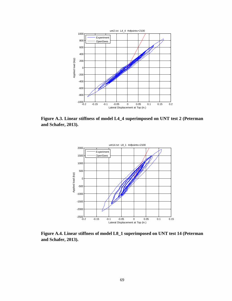
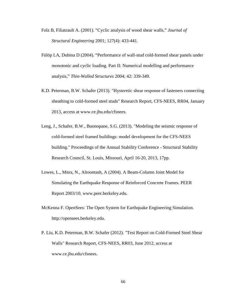
Figure A.3. Linear stiffness of model L4_4 superimposed on UNT test 2 (Peterman and Schafer, 2013).
Figure A.4. Linear stiffness of model L8_1 superimposed on UNT test 14 (Peterman and Schafer, 2013).
-0.2 -0.15 -0.1 -0.05 0 0.05 0.1 0.15 0.2-1000
-800
-600
-400
-200
0
200
400
600
800
1000
Lateral Displacement at Top (in.)
App
lied
load
(kip
)
unt2.txt L4_4 #ofpoints=2100
ExperimentOpenSees
-0.2 -0.15 -0.1 -0.05 0 0.05 0.1 0.15-2500
-2000
-1500
-1000
-500
0
500
1000
1500
2000
Lateral Displacement at Top (in.)
App
lied
load
(kip
)
unt14.txt L8_1 #ofpoints=2100
ExperimentOpenSees
69
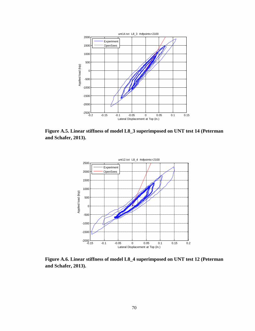
Figure A.5. Linear stiffness of model L8_3 superimposed on UNT test 14 (Peterman and Schafer, 2013).
Figure A.6. Linear stiffness of model L8_4 superimposed on UNT test 12 (Peterman and Schafer, 2013).
-0.2 -0.15 -0.1 -0.05 0 0.05 0.1 0.15-2500
-2000
-1500
-1000
-500
0
500
1000
1500
2000
Lateral Displacement at Top (in.)
App
lied
load
(kip
)
unt14.txt L8_3 #ofpoints=2100
ExperimentOpenSees
-0.15 -0.1 -0.05 0 0.05 0.1 0.15 0.2-2000
-1500
-1000
-500
0
500
1000
1500
2000
2500
Lateral Displacement at Top (in.)
App
lied
load
(kip
)
unt12.txt L8_4 #ofpoints=2100
ExperimentOpenSees
70
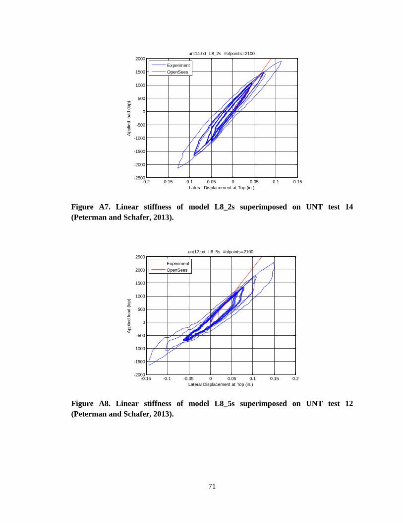
Figure A7. Linear stiffness of model L8_2s superimposed on UNT test 14 (Peterman and Schafer, 2013).
Figure A8. Linear stiffness of model L8_5s superimposed on UNT test 12 (Peterman and Schafer, 2013).
-0.2 -0.15 -0.1 -0.05 0 0.05 0.1 0.15-2500
-2000
-1500
-1000
-500
0
500
1000
1500
2000
Lateral Displacement at Top (in.)
App
lied
load
(kip
)
unt14.txt L8_2s #ofpoints=2100
ExperimentOpenSees
-0.15 -0.1 -0.05 0 0.05 0.1 0.15 0.2-2000
-1500
-1000
-500
0
500
1000
1500
2000
2500
Lateral Displacement at Top (in.)
App
lied
load
(kip
)
unt12.txt L8_5s #ofpoints=2100
ExperimentOpenSees
71