Fast Local Search and Guided Local Search and Their Application to British Telecom’s Workforce Scheduling Problem

Edward Tsang & Chris Voudouris

Technical Report CSM-246Department of Computer Science

University of EssexColchester CO4 3SQ

email: {voudcx, edward}@uk.ac.essex

August 1995

Abstract

This paper reports a Fast Local Search (FLS) algorithm which helps to improve the efficiencyof hill climbing and a Guided Local Search (GLS) Algorithm which is developed to help localsearch to escape local optima and distribute search effort. To illustrate how these algorithmswork, this paper describes their application to British Telecom’s workforce scheduling prob-lem, which is a hard real life problem. The effectiveness of FLS and GLS are demonstrated bythe fact that they both out-perform all the methods applied to this problem so far, whichinclude simulated annealing, genetic algorithms and constraint logic programming.

I. Introduction

Due to their combinatorial explosion nature, many real life constraint optimization problemsare hard to solve using complete methods such asbranch & bound[17, 14, 21, 23]. One wayto contain the combinatorial explosion problem is to sacrifice completeness. Some of the bestknown methods which use this strategy arelocal search methods, the basic form of whichoften referred to ashill climbing. The problem is seen as an optimization problem according toan objective function (which is to be minimized or maximized). The strategy is to define aneighbourhood function which maps every candidate solution (often called astate) to a set ofother candidate solutions (which are calledneighbours). Then starting from a candidate solu-tion, which may be randomly or heuristically generated, the search moves to a neighbourwhich is ‘better’ according to the objective function (in a minimization problem, a betterneighbour is one which is mapped to a lower value by the objective function). The search ter-minates if no better neighbour can be found. The whole process can be repeated from differentstarting points.

One of the main problems with hill climbing is that it may settle in local optima — stateswhich are better than all the neighbours but not necessarily the best possible solution. To over-

2

come that, methods such assimulated annealing [1, 7, 20] andtabu search [10, 11, 12] havebeen proposed. In this paper, we present a method, calledGuided Local Search (GLS), toguide local search to escape local optima. Like tabu search, this method also allows the soft-ware engineer to build knowledge into the algorithm to guide the search towards areas whichappear to be more promising.

A factor which limits the efficiency of a hill climbing aglorithm is the size of the neighbour-hood. If there are many neighbours to consider, then if the search takes many steps to reach alocal optima, and/or each evaluation of the objective function requires a nontrivial amount ofcomputation, then the search could be very costly. In this paper, we present a method, whichwe calledFast Local Search (FLS) to restrict the neighbourhood. The intention is to ignoreneighbours which are unlikely to lead to fruitful hill-climbs in order to improve the efficiencyof a search.

We shall illustrate these two algorithms by using a real life scheduling problem as an example.We shall also use this example problem to demonstrate the effectiveness and efficiency ofthese two algorithms. In the next section, we shall explain this example problem.

II. BT’s Workforce Scheduling Problem

The problem is to schedule a number of engineers to a set of jobs, minimizing total costaccording to a function which is to be explained below. Each job is described by a triple:

(Loc, Dur, Type) (1)

whereLoc is the location of the job (depicted by itsx andy coordinates),Dur is the standardduration of the job andType indicates whether this job must be done in the morning, in theafternoon, as the first job of the day, as the last job of the day, or “don’t care”.

Each engineer is described by a 5-tuple:

(Base, ST, ET, OT_limit, Skill) (2)

whereBase is thex andy coordinates at which the engineer locates,ST andET are this engi-neer’s starting and ending time,OT_limit is his/her overtime limit, andSkill is a skill factorbetween 0 and 1 which indicates the fraction of the standard duration that this engineer needsto accomplish a job. In other words, the smaller thisSkill factor, the less time this engineerneeds to do a job. If an engineer with skill factor 0.9 is to serve a job with duration (Dur) 20,say, then this engineer would actually take 18 minutes to finish the job.

The cost function which is to be minimized is defined as follows:

Total Cost = (3)

where: NoT = number of engineers;NoJ = number of jobs;TCi = Travelling Cost of engineeri;OTi = Overtime of engineeri;Durj = Duration of jobj;UFj = 1 if job j is not served; 0 otherwise;Penalty = constant (which is set to 60 in the tests)

TCii 1=

NoT

∑ OTi2

i 1=

NoT

∑ Durj Penalty+( ) UFj×j 1=

NoJ

∑+ +

3

The travelling cost between (x1, y1) to (x2, y2) is defined as follows:

if ;

otherwise. (4)

Here is the absolute difference betweenx1 andx2, and is the absolute differencebetweeny1 andy2. The greater of thex andy differences is halved before summing. Engineersare required to start from and return to their bases everyday. An engineer may be assignedmore jobs than he/she can finish.

III. Fast Local Search Applied to Workforce Scheduling

III.1. Representation of candidate solutions and hill climbing

To tackle BT’s workforce scheduling problem, we represent a candidate solution (i.e. a possi-ble schedule) by a permutation of the jobs. Each permutation is mapped into a schedule usingthe following (deterministic) algorithm:

ProcedureEvaluation (input: one particular permutation of jobs)

1. For each job, order the qualified engineers in ascending order of the distancesbetween their bases and the job (such orderings only need to be computedonce and recorded for evaluating other permutations)

2. Process one job at a time, following their ordering in the input permutation.For each jobx, try to allocate it to an engineer according to the ordered list ofqualified engineers:2.1. to check if engineerg can do jobx, makex the first job ofg; if that fails

to satisfy any of the constraints, make it the second job ofg, and so on;2.2. if job x can be fitted into engineerg’s current tour, then try to improve

g’s new tour (now withx in it): the improvement is done by a simple 2-opting algorithm (see e.g. [2]), modified in the way that only bettertours which satisfy the relevant constraints will be accepted;

2.3. if job x cannot be fitted into engineerg’s current tour, then consider thenext engineer in the ordered list of qualified engineers forx; the job isunallocated if it cannot fit into any engineer’s current tour.

3. The cost of the input permutation, which is the cost of the schedule thus cre-ated, is returned.

Given a permutation, hill climbing is performed in a simple way: a pair of jobs are looked at ata time. Two jobs are swapped to generate a new permutation if the new permutation is evalu-ated (using theEvaluation procedure above) to a lower cost than the original permutation.

The starting point of the hill climbing is generated heuristically and deterministically: the jobsare ordered by the number of qualified engineers for them. Jobs which can be served by thefewest number of qualified engineers are placed earlier in the permutation.

TC x1 y1,( ) x2 y2,( ),( )∆x 2⁄ ∆y+

8= ∆x ∆y>

∆y 2⁄ ∆x+8

=

∆x ∆y

4

III.2. Fast Hill climbing

So far we have defined an ordinary hill climbing algorithm. Each state in this algorithm hasO(n2) neighbours, wheren is the number of jobs in the workforce scheduling problem. Thefast local search is a general strategy which allows us to restrict the neighbourhood, and con-sequently improve the efficiency of the hill climbing. We shall explain here how it is appliedto the workforce scheduling problem. Later we shall explain that this technique can be (andhas successfully been) generalized to other problems.

To apply the fast local search to workforce scheduling, each job permuation position is associ-ated with it anactivation bit, which takes binary values (0 and 1). These bits are manipulatedin the following way:

1. All the activation bits are set to 1 (or “on”) when hill climbing starts;

2. the bit for job permutation positionx will be switched to 0 (or “off”) if everypossible swap between the job at positionx and another job under the currentpermutation has been considered, but no better permutation has been found;

3. the bit for job permutation positionx will be switched to 1 wheneverx isinvolved in a swap which has been accepted.

During hill climbing, only those job permutation positions which activation bits are 1 will beexamined for swapping. In other words, positions which have been examined for swappingbut failed to produce a better permutation will be heuristically ignored. Positions whichinvolved in a successful swap recently will be examined more. The overall effect is that thesize of neighbourhood is greatly reduced and resources are invested in examining swapswhich are more likely to produce better permutations.

IV. Guided Local Search Applied to Workforce Scheduling

IV.1. The GLS algorithmLike all other hill climbing algorithms, FLS suffers from the problem of settling in localoptima. Guided local search (GLS) is a method for escaping local optima. GLS is built uponour experience in a connectionist method called GENET (it is a generalization of the GENETcomputation models) [27, 6, 26].

GLS is a algorithm for modifying local search algorithms. The basic idea is thatcosts andpen-alty values are associated to selected features of the candidate solutions. Selecting such fea-tures in an application is not difficult because the objective function is often made up of anumber of features in the candidate solutions. If the costs should normally take their valuesfrom the objective function. The penalties are initialized to 0.

Given an objective functiong which maps every candidate solutions to a numerical value, wedefine a functionh which will be used by the local search algorithm (replacingg).

h(s) = g(s) + (5)

wheres is a candidate solution,λ is a parameter to the GLS algorithm,F is the number of fea-tures,pi is the penalty for featurei (which are initialized to 0) andIi is an indication of whetherthe candidate solutions exhibits featurei:

Ii (s) = 1 if s exhibits featurei; 0 otherwise. (6)

λ pi I i s( )⋅i 1 F,=∑

5

When the local search settles on a local optimum, the penalty of some of the features associ-ated to this local optimum is increased (to be explained below). This has the effect of changingthe objective function (which defines the “landscape” of the local search) and driving thesearch towards other candidate solutions. The key to the effectiveness of GLS is in the waythat the penalties are imposed.

Our intention is to penalize “bad features”, or features which “matter most”, when a localsearch settles in a local optima. The feature which has high cost affects the overall cost more.Another factor which should be considered is the current penalty value of that feature. Wedefine the utility of penalizing featurei, utili, under a local optimums* , as follows:

utili(s*) = Ii (s*) × (7)

In other words, if a feature is not exhibited in the local optimum, then the utility of penalizingit is 0. The higher the cost of this feature, the greater the utility of penalizing it. Besides, themore times that it has been penalized, the greater (1 +pi) becomes, and therefore, the lowerthe utility of penalizing it again.

In a local optimum, the feature(s) with the greatestutil value will be penalized. This is done byadding 1 to its penalty value:

pi = pi + 1 (8)

The λ parameter in the GLS algorithm is used to adjust the weight of penalty values in theobjective function. As it will be shown later, results in applying GLS to the workforce sched-uling problem is not very sensitive to the setting of this parameter.

By taking cost and the current penalty into consideration in selecting the feature to penalize,we are distributing the search effort in the search space. Candidate solutions which exhibit“good features”, i.e. features involving lower cost, will be given more effort in the search, butpenalties may lead the search to explore candidate solutions which exhibit features with highercost. The idea of distributing search effort, which plays an important role in the success ofGLS, is borrowed from Operations Research, e.g. see Koopman [16] and Stone [22].

Following we shall describe the general GLS procedure:

ProcedureGLS (input: an objective functiong and a local search strategyL)

1. Generate a starting candidate solution randomly or heuristically;

2. Initialize all the penalty values (pi) to 0;

3. Repeat the following until a termination condition (e.g. a maximum numberof iterations or a time limit) has been reached:3.1. Perform local search (usingL) according to the functionh (which isg

plus the penalty values, as defined above) until a local optimumM hasbeen reached;

3.2. For each featurei which is exhibited inM computeutili = ci / (1 +pi)3.3. Penalize every featurei such thatutili is maximum:pi = pi + 1;

4. Return the best candidate solution found so far according to the objectivefunctiong.

ci

1 pi+

6

IV.2. GLS applied to BT’s workforce scheduling problem

To apply GLS to a problem, we need to identify the objective function and a local search algo-rithm. In earlier sections, we have described the objective function and a local search algo-rithm, FLS, for BT’s workforce scheduling problem.

Our next task is to define solution features to penalize. In the workforce scheduling problem,the inability to serve jobs incurs a cost, which plays an important part in the objective functionwhich is to be minimized. Therefore, we intend to penalize the inability to serve a job in a per-mutation. To do so, we associate a penalty value to each job. The travelling cost is taken careof by the ordering of engineers by their distance to the jobs in the local search described in theEvaluation procedure above as well as 2-opting. (If the travelling cost in this problem is foundto play a role as important as unallocated jobs, we could associate a penalty to the assignmentof each jobx to each engineerg, with the cost of this feature reflecting the travelling cost. Thispenalty is increased if the schedule in a local minimum uses engineerg to do jobx.) Integratedinto GLS, FLS will switch on (i.e. switching from 0 to 1) the activation bits associated to thepositions where the penalized jobs currently lie.

It may be worth noting that since the starting permutation is generated heuristically, and hillclimbing is performed deterministically, the application of FLS and GLS presented here do notinvolve any randomness as most local search applications do.

V. Experimental Results

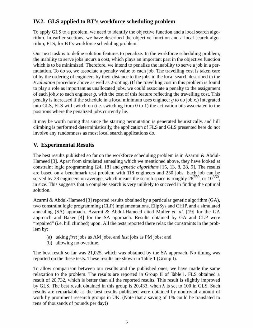
The best results published so far on the workforce scheduling problem is in Azarmi & Abdul-Hameed [3]. Apart from simulated annealing which we mentioned above, they have looked atconstraint logic programming [24, 18] andgenetic algorithms [15, 13, 8, 28, 9]. The resultsare based on a benchmark test problem with 118 engineers and 250 jobs. Each job can beserved by 28 engineers on average, which means the search space is roughly 28250, or 10360,in size. This suggests that a complete search is very unlikely to succeed in finding the optimalsolution.

Azarmi & Abdul-Hameed [3] reported results obtained by a particular genetic algorithm (GA),two constraint logic programming (CLP) implementations, ElipSys and CHIP, and a simulatedannealing (SA) approach. Azarmi & Abdul-Hameed cited Mulleret. al. [19] for the GAapproach and Baker [4] for the SA approach. Results obtained by GA and CLP were“repaired” (i.e. hill climbed) upon. All the tests reported there relax the constraints in the prob-lem by:

(a) takingfirst jobs as AM jobs, andlast jobs as PM jobs; and (b) allowing no overtime.

The best result so far was 21,025, which was obtained by the SA approach. No timing wasreported on the these tests. These results are shown in Table 1 (Group I).

To allow comparison between our results and the published ones, we have made the samerelaxation to the problem. The results are reported in Group II of Table 1. FLS obtained aresult of 20,732, which is better than all the reported results. This result is slightly improvedby GLS. The best result obtained in this group is 20,433, whenλ is set to 100 in GLS. Suchresults are remarkable as the best results published were obtained by nontrivial amount ofwork by prominent research groups in UK. (Note that a saving of 1% could be translated totens of thousands of pounds per day!)

7

Table 1: Results obtained in BT’s benchmark workforce scheduling problem

Algorithms Total costCpu time

(sec)Travelcost

Cost(number) ofunallocated

jobs

over-timecost

Group I: Best results reported in the literature (no overtime allowed):

GA + repair 23,790 N.A. N.A. N.A. (67) disallow

22,570 N.A. N.A. N.A. (54) disallow

CLP — ElipSys + repair 21,292 N.A. 4,902 16,390 (53) disallow

CLP — CHIP + repair 22,241 N.A. 5,269 16,972 (48) disallow

SA 21,025 N.A. 4,390 16,660 (56) disallow

Group II: Best results on FLS and GLS withovertime disallowed:

Fast Local Search (FLS) 20,732 1,242 4,608 16,124 (49) disallow

Fast GLS

λ = 10 20,556 5,335 4,558 15,998 (48) disallow

λ = 20 20,497 7,182 4,533 15,864 (49) disallow

λ = 30 20,486 6,756 4,676 15,810 (50) disallow

λ = 40 20,490 5,987 4,743 15,747 (48) disallow

λ = 50 20,450 3,098 4,535 15,915 (49) disallow

λ = 100 20,433 9,183 4,707 15,726 (48) disallow

Group III: Best results on FLS and GLS, with a maximum of 10 minutesovertime allowed:

Fast Local Search (FLS) 20,224 1,244 4,651 15,448 (51) 125

Fast GLS

λ = 10 20,124 4,402 4,663 15,329 (50) 132

λ = 20 19,997 4,102 4,648 15,209 (49) 140

λ = 30 20,000 2,788 4,690 15,155 (48) 155

λ = 40 20,070 4,834 4,727 15,194 (48) 149

λ = 50 20,055 2,634 4,690 15,197 (49) 168

λ = 100 20,132 2,962 4,779 15,152 (48) 201

Notes:1. GA, CLP and SA results from Azarmi & Abdul-Hameed [3], Mulleret. al. [19] and

Baker [4];2. FLS and GLS are implemented in C++, all results obtained from a DEC Alpha 3000/600

175MHz machine; results are available in http://cswww.essex.ac.uk/CSP/wfs;3. The benchmark problem, which has 118 engineers and 250 jobs, is obtained from British

Telecom Research Laboratories, UK.

8

In the objective function, the overtime term is squared. This discourages overtime in sched-ules, but it does not mean that a good schedule cannot have overtime. We tried to restate thisconstraint, but gave each engineer a limit in overtime. The best result, which were found inlimiting overtime to 10 minutes per engineer, is shown in Group III of Table 1. FLS in thisgroup obtained a result of 20,224, which was better than all the results in Group II. The bestresult in Group III, which is 19,997, was found by GLS whenλ was set to 20.

The λ parameter is the only parameter that needs to be set in GLS (there are relatively moreparameters to set in both GA and SA). The above test results show that the total cost is not ter-ribly sensitive to the setting ofλ.

Test data1 and results reported in this paper by FLS and GLS are included in Essex’s worldwide web (http://cswww.essex.ac.uk/CSP/wfs) for reference and verification.

VI. Discussion

In BT’s workforce scheduling problem, anactivation bit is associated to each job permutationpostion. Although the definition of activation bits in FLS is domain dependent, it is not diffi-cult to define them in an application. Hints can often be obtained from the objective functionor the representation of candidate solutions.

FLS is a generalization of Bentley’sapproximate 2-opting algorithm [5], which is applied tothe travelling salesman problem (TSP). Voudouris & Tsang [26] report the successful applica-tion of FLS and GLS in the TSP. Apart from these prolems, FLS has been applied successfullyto the radio link frequency assignment problem, which will be reported in detail in anotheroccasion (this problem and early results were reported in Voudouris & Tsang [25]).

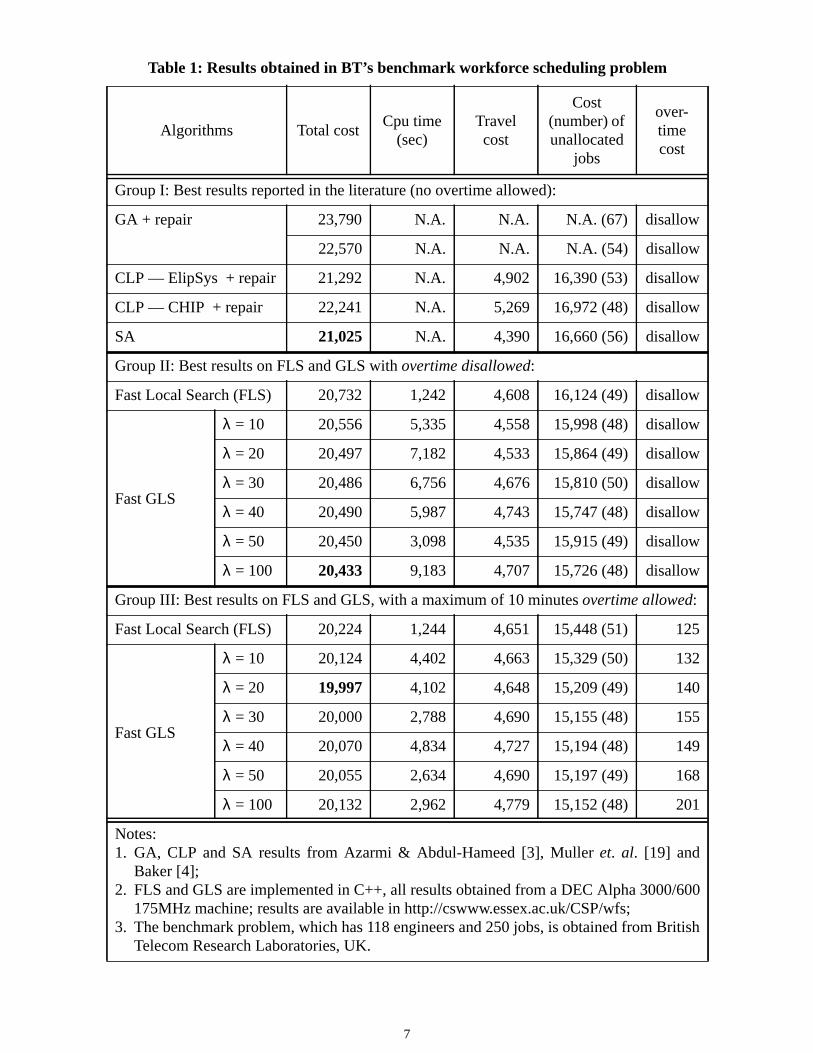
To evaluate the role of the activation bits in the efficiency of FLS, we compare FLS with alocal search algorithm which uses the same hill climbing strategy as FLS, but without usingactivation bits to reduce its neighbourhood (we refer to this algorithm as LS). The results areshown in Table 2.

1. with the permission of British Telecom

Table 2: Evalutation of the efficiency of FLS

AlgorithmsTotalcost

Cputime(sec)

speedup by FLSin cputime

Travel cost

Cost(number) ofunallocated

jobs

over-timecost

No overtimeallowed

FLS 20,732 1,24216 times

4,608 16,124 (49) disallow

LS 20,788 20,056 4,604 16,184 (50) disallow

Max. 10 min.OT allowed

FLS 20,224 1,24420 times

4,651 15,448 (51) 125

LS 20,124 25,195 4,595 15,358 (48) 171

Notes: Local Search (LS) use the same hill climbing strategy as FLS, but no activation bitsare used; Both aglorithms implemented in C++, all results obtained from a DEC Alpha3000/600 175MHz machine

9

When no overtime is allowed, FLS runs 16 times faster than LS, which converged to a slightlyworse local minimum. When a maximum of 10 minutes is allowed for overtime, FLS runs 20times faster than LS, though LS produced a slightly better result. Our conclusion is that theactivation bits help to speed up FLS significantly and there is no convincing evidence thatquality of results has been sacrificed in the workforce scheduling problem.

In BT’s workforce scheduling problem, penalties are associated to each job, because they arethe subject of allocation. The selection of features to be penalized is (like the definition of acti-vation bits) not difficult. It can often be done through observation in the objective function.Bits can be associated to elements which make up the total cost. (In fact, a similar exercise isoften done in genetic algorithms in defining building blocks in a representation.)

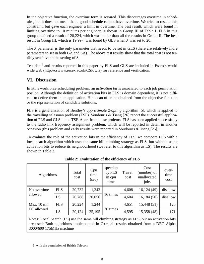
We have also experimented with random starting permutations and a starting permutation withthe jobs ordered by the ratio between their durations and the number of qualified engineers.Their results are shown in Table 3.

In Table 3, an (almost) arbitraryλ value of 100 has been chosen to give the readers more infor-mation about the sensitivity of GLS over this parameter (though this was not the parameterunder which the best result were generated when overtime was allowed). Results in Table 3shows that the result of FLS can be affected by the initial ordering of the job, though even theworse result is comparable with those reported in the literature. However, Fast GLS is rela-tively insensitive to it — all the results of GLS are better than the best result reported in the lit-erature. This helps to show the robustness of GLS. More evidence of the effectiveness of GLSwill be given in other occasions.

VII. Concluding Summary

In this paper, we have described two general local algorithms, namely the fast local search(FLS) algorithms and the guided local search (GLS) algorithm, for tackling constraint optimi-zation problems. We have demonstrated their effectiveness in a case study using British Tele-com’s workforce scheduling problem. On the benchmark problem, our algorithms obtainedresults convincingly better than those published, which include simulated annealing, geneticalgorithms and constraint logic programming.

The FLS algorithms is designed to speed up local search by restricting the neighbourhood tothose which are more likely to contain better neighbours. This allows one to speed up a hill

Table 3: Ordering heuristics used in starting permutation

Heuristics used in generatingstarting permutation

InitialCost

After FLS After Fast GLS

cost cpu sec cost cpu sec

Random ordering 25,886 21,204 767 20,287 7,639

Job duration / # of qualified eng. 23,828 20,286 903 20,187 2,468

# of qualified engineers 22,846 20,224 1,218 20,132 2,962

Notes: a maximum of 10 minutes is allowed in overtime; a maximum of 500 penalty cyclesis allowed in GLS, which usesλ = 100; all programs implemented in C++; all resultsobtained from a DEC Alpha 3000/600 175MHz machine

10

climbing search. The GLS algorithm helps local search to escape local optima by adding apenalty term in the objective function. The penalties also help the search to distribute its effortaccording to the promise of the selected features in candidate solutions.

Acknowledgement

The Computer Service Department provided the DEC Alpha machines. The benchmark prob-lem was obtained from British Telecom (BT) Research Laboratories. Edward Tsang was sup-ported by a BT Short Term Research Fellowship in 1992, under the guidance of BarryCrabtree. Chris Voudouris is employed by the EPSRC funded project, ref GR/H75275.

11

References

[1] E. Aarts and J. Korst,Simulated Annealing and Boltzmann Machines, JohnWiley & Sons, 1989.

[2] A.V. Aho, J.E. Hopcroft, and J.D. Ullman,Data structures and algorithms,Addison-Wesley, 1983.

[3] N. Azarmi and W. Abdul-Hameed, “Workforce scheduling with constraintlogic programming”,British Telecom Technology Journal, Vol.13, No.1,January, 81-94 (1995).

[4] S. Baker, “Applying simulated annealing to the workforce managementproblem”, ISR Technical Report, British Telecom Laboratories, MartleshamHeath, Ipswich (1993).

[5] J.J. Bentley, “Fast algorithms for geometric traveling salesman problems”,ORSA Journal on Computing, Vol.4, 387-411 (1992).

[6] A. Davenport, E.P.K. Tsang, C.J. Wang and K. Zhu, “GENET: a connection-ist architecture for solving constraint satisfaction problems by iterativeimprovement”,Proc., 12th National Conference for Artificial Intelligence(AAAI), 325-330 (1994).

[7] L. Davis (ed.),Genetic algorithms and simulated annealing, Research notesin AI, Pitman/Morgan Kaufmann, 1987.

[8] L. Davis (ed.),Handbook of genetic algorithms, Van Nostrand Reinhold,1991.

[9] A.E. Eiben, P-E. Raua, and Zs. Ruttkay, “Solving constraint satisfactionproblems using genetic algorithms”, Proc., 1st IEEE Conference on Evolu-tionary Computing, 543-547 (1994).

[10] F. Glover, “Tabu search Part I”,ORSA Journal on Computing 1, 109-206(1989).

[11] F. Glover, “Tabu search Part II”,ORSA Journal on Computing 2, 4-32(1990).

[12] F. Glover, E. Taillard, and D. de Werra, “A user’s guide to tabu search”,Annals of Operations Research, Vol.41, 1993, 3-28 (1993).

[13] D.E. Goldberg,Genetic algorithms in search, optimization, and machinelearning, Addison-Wesley Pub. Co., Inc., 1989.

[14] P.A.V. Hall, “Branch and bound and beyond”,Proc. International JointConference on AI, 641-650 (1971).

[15] J.H. Holland,Adaptation in natural and artificial systems, University ofMichigan press, Ann Arbor, MI, 1975.

[16] B.O. Koopman, “The theory of search, part III, the optimum distribution ofsearching effort”,Operations Research, Vol.5, 1957, 613-626 (1957).

[17] E.W. Lawler and D.E. Wood, “Branch-and-bound methods: a survey”,

12

Operations Research 14, 699-719 (1966).

[18] J. Lever, M. Wallace, and B. Richards, “Constraint logic programming forscheduling and planning”,British Telecom Technology Journal, Vol.13,No.1., 73-80 (1995).

[19] C. Muller, E.H. Magill, and D.G. Smith, “Distributed genetic algorithms forresource allocation”, Technical Report, Strathclyde University, Glasgow(1993).

[20] R.H.J.M. Otten and L.P.P.P. van Ginneken,The annealing algorithm, Klu-wer Academic Publishers, 1989.

[21] E. M. Reingold, J. Nievergelt, and N. Deo,Combinatorial algorithms: the-ory and practice, Englewood Cliffs, N.J., Prentice hall, 1977.

[22] L.D. Stone, “The process of search planning: current approaches and contin-uing problems”,Operations Research, Vol.31, 207-233 (1983).

[23] E.P.K. Tsang, “Scheduling techniques — a comparative study”,British Tele-com Technology Journal, Vol.13, No.1, 16-28 (1995).

[24] P. van Hentenryck,Constraint satisfaction in logic programming, MITPress, 1989.

[25] C. Voudouris and E.P.K. Tsang, “The tunnelling algorithm for partial con-straint satisfaction problems and combinatorial optimization problems”,Technical Report CSM-213, Department of Computer Science, Universityof Essex (1994).

[26] C. Voudouris and E.P.K. Tsang, “Guided Local Search”, Technical ReportCSM-247, Department of Computer Science, University of Essex (1995).

[27] C.J. Wang and E.P.K. Tsang, “Solving constraint satisfaction problemsusing neural-networks”,Proceedings of IEE Second International Confer-ence on Artificial Neural Networks, 295-299 (1991).

[28] T. Warwick and E.P.K. Tsang, “Using a genetic algorithm to tackle the proc-essors configuration problem”,Symposium on Applied Computing (1994).