fast incremental maintenance of approximate histograms · fast incremental maintenance of...

Fast Incremental Maintenance of Approximate Histograms

Phillip B. Gibbons Yossi Matias Viswanath Poosala

Bell Laboratories, 600 Mountain Avenue, Murray Hill NJ 07974 { gibbons,matias,poosala} @research.bell-labscorn

Abstract

Many commercial database systems maintain histograms to summarize the contents of large relations and permit efficient estimation of query result sizes for use in query optimizers. Delay- ing the propagation of database updates to the histogram often introduces errors in the estimation. This paper presents new sampling-based approaches for incremental maintenance of approximate histograms. By scheduling updates to the histogram based on the updates to the database, our techniques are the first to maintain histograms effectively up-to-date at all times and avoid computing overheads when unnecessary. Our techniques provide highly-accurate approximate histograms belonging to the equi-depth and Com- pressed classes. Experimental results show that our new approaches provide orders of magnitude more accurate estimation than previous approaches.

An important aspect employed by these new approaches is a backing sample, an up-to-date random sample of the tuples currently in a relation. We provide efficient solutions for maintaining a uniformly random sample of a relation in the presence of updates to the relation. The backing sample techniques can be used for any other application that relies on random samples of data.

1 Introduction

Most DBMSs maintain a variety of statistics on the contents of the database relations in order to estimate various quantities, such as selectivities within cost-based query optimizers. These statistics are typically used to approximate

Permission to copy without jke all or part of this material is granted provided that the copies are not made or distributedfor direct commercial advantage, the VWB copyright notice and the title af the publication and its date appear: and notice is given that copying is by permission of the %-r-y Large Data Base Endowment. 7i) copy otherwise, or to republish, requires a fee and/or special permission from the Endowment.

Proceedings of the 23rd VLDB Conference Athens, Greece, 1997

the distribution of data in the attributes of various database relations. It has been established that the validity of the optimizer’s decisions may be critically affected by the quality of these approximations [1, 41. This is becoming particularly evident in the context of increasingly complex queries (e.g., data analysis queries).

Probably the most common technique used in practice for selectivity estimation is maintaining histograms on the frequency distribution of an attribute. A histogram groups attribute values into “buckets” (subsets) and approximates true attribute values and their frequencies based on summary statistics maintained in each bucket [q. For most real-world databases, there exist histograms that produce low-error estimates while occupying reasonably small space (of the order of 1K bytes in a catalog) [6]. Histograms are used in DB2, Informix, Ingres, Oracle, Microsoft SQL Server, Sybase, and Teradata. They are also being used in other areas, e.g., parallel join load balancing [7] toprovidevarious estimates.

Histograms are usually precomputed on the underlying data and used without much additional overheads inside the query optimizer. A drawback of using precomputed histograms is that they may get outdated when the data in the database is modified, and hence introduce significant errors in estimations. On the other hand, it is clearly impractical to compute a new histogram after every update to the database. Fortunately, it is not necessary to keep the histograms perfectly up-to-date at all times, because they are used only to provide reasonably accurate estimates (typically within l-10%). Instead, one needs appropriate schedules and algorithms for propagating updates to histograms, so that the database performance is not affected.

Despite the popularity of histograms, most issues related to their maintenance have not been studied in the literature. Most of the work so far has focused on proper bucketizations of values in order to enhance the accuracy of histograms, and assumed that the database is not being modified. In our earlier work, we have introduced several classes of histograms that offer high accuracy for various estimation problems [8]. We have also provided efficient sampling- based methods to construct various histograms, but ignored the problem of maintaining histograms. In a more general context, we can view histograms as materialized views, but they are different in two aspects. First, during utilization,

466

they are typically maintained in main memory, which im- plies more constraints on space. Second, they need to be maintained only approximately, and can therefore be considered as cached approximate materialized views. We are not aware of any prior work on approximate materialized views.

The only approach used to date for histogram updates, which is followed in nearly all commercial systems, is to recompute histograms periodically (e.g., every night). This approach has two disadvantages. First, any significant updates to the data between two recomputations could cause poor estimations in the optimizer. Second, since the histograms are recomputed from scratch by discarding the old histograms, the recomputation phase for the entire database is computationally very intensive.

In this paper, we present fast and effective procedures for maintaining two histogram classes used extensively in DBMSs: equi-depth histograms (which are used in most DBMSs) and Compressed histograms (used in DB2). As a key component of our approach, we introduce the notion of a “backing sample”, which is a random sample of the tuples in a relation, that is kept up-to-date in the presence of updates. We demonstrate important advantages gained by using a backing sample and present algorithms for its maintenance. We conducted an extensive set of experiments studying these techniques which confirm the theoret- ical findings and show that with a small amount of additional storage and CPU resources, these techniques maintain histograms nearly up-to-date at all times.

Due to the limited space, the proofs of all theorems in this paper, as well as many technical details, are omitted and can be found in the full version of this paper [3].

2 Histograms and their maintenance

The domain 2) of an attribute X is the set of all possible values of X and the value set V (C 2)) for a relation R is the set of values of X that are present in R. Let V = {vi : 1 5 i 5 IVl}, where zii < vj when i < j. The frequency fi of vi is the number of tuples t E R with t .X = Q. The data distribution of X (in R) is the set of pairs 7 = {(VI, f~), (~2, f2), . . . , (~1~1, fpl)l.

A histogramon attribute X is constructed by partitioning the datadistribution 7 into p (2 1) mutually disjoint subsets called buckets and approximating the values and frequencies in each bucket in some common fashion. Typically, a bucket is assumed to contain either all m values in 2) between the smallest and largest values in that bucket (the bucket’s range), or just rE 5 m equi-distant values in the range, where L is actual number of values in the bucket. The former is known as the continuous value assumption [9], and the latter is known as the uniform spread assumption [S]. Let fn be the number of tuples t E R with t.X = v for some value v in bucket B. The frequencies for values in a bucket B are approximated by their averages; i.e., by either f~/m

Different classes of histograms can be obtained by using different rules for partitioning values into buckets. In this paper, we focus on two important classes of histograms, namely the equi-depth and Compressed (simply called Compressed in this paper) classes. In an equi-depth (or equi-height) histogram, contiguous ranges of attribute values are grouped into buckets such that the number of tuples, fB, in each bucket B is the same. In a Compressed histogram [8], the n highest frequencies are stored separately in n singleton buckets; the rest are partitioned as in an equi- depth histogram. In our target Compressed histogram, the value of n adapts to the data distribution to ensure that no singleton bucket can fit within an equi-depth bucket and yet no single value spans an equi-depth bucket. We have shown in our earlier work [8] that Compressed histograms are very effective in approximating distributions of low or high skew.

Equi-depth histograms are used in one form or another in nearly all commercial systems, except DB2 which uses the more accurate Compressed histograms.

Histogram storage. For both equi-depth and Compressed histograms, we store for each bucket B the largest value in the bucket, B.maxval, and a count, Bcount, that equals or approximates fB. When using the histograms to estimate range selectivities, we apply the uniform spread assumption for singleton buckets and the continuous value assumption for equi-depth buckets.

2.1 Approximate histograms

Let ‘H be the class C histogram, or C-histogram, on attribute X for a relation R. When R is modified, the accuracy of 31 is affected in two ways: 1-I may no longer be the cor- rect C-histogram on the updated data (Class Error) and ‘H may contain inaccurate information about X (Distribution Error).

For a given attribute, an approximate C-histogram provides an approximation to the actual C-histogram for the relation. The quality of the approximation can be evaluated according to various error metrics defined based on the class and distribution errors.

The pcount error metric. An example of a distribution error metric, relevant to many histogram types, reflects the accuracy of the counts associated with each bucket. For example, when R is modified, but the histogram is not, then there may be buckets B with B.count # fB; the difference between fB and B.count is the approximation error for B. We consider the error metric, pcount, defined as follows:

’ ’ &B, - Bi.count)z , Pcount = z 3

@ i=l (1)

where N is the number of tuples in R and /I is the number of buckets. This is the standard deviation of the bucket

467

counts from the actual number of elements in each bucket, normalized with respect to the mean bucket count (N/P).

2.2 Incremental histogram maintenance

There are two components to our incremental approach: (i) maintaining a backing sample, and (ii) a framework for maintaining an approximate histogram that performs a few program instructions in response to each update to the database,’ and detects when the histogram is in need of an adjustment of one or more of its bucket boundaries. Such adjustments make use of the backing sample. There is a fundamental distinction between the backing sample and the histogram it supports: the histogram is accessed far more frequently than the sample and uses less memory, and hence it can be stored in main memory while the sample is likely stored on disk. Figure 1 shows typical sizes of various entities relevant to our discussion.

Figure 1: Typical sizes of various entities

Incremental histogram maintenance was previously studied in [2], for the important case of a high-biased histogram, which is a Compressed histogram with /3 - 1 buckets devoted to the p - 1 most frequent values, and 1 bucket devoted to all the remaining values. This algorithm did not use the approach described above - for example, no backing sample was maintained or used.

3 Backing sample A backing sample is a uniform random sample of the tuples in a relation that is kept up-to-date in the presence of updates to the relation.

We argue that maintaining a backing sample is useful for histogram computation, selectivity estimation, etc. In most sampling-based estimation techniques, whenever a sample of size n is needed, either the entire relation is scanned to extract the sample, or several random disk blocks are read. In the latter case, the tuples in a disk block may be highly correlated, and hence to obtain a truly random sample, n disk blocks must be read. In contrast, a backing sample can be stored in consecutive disk blocks, and can therefore be scanned by reading sequential disk blocks. Moreover, for each tuple in the sample, only the unique row id and the

‘To further reduce the overhead of our approach, the few program instructions can be performed only for a random sample of the database updates (as discussed in Section 6.2).

attribute(s) of interest are retained. Thus the entire sample can be stored in only a few disk blocks, for even faster retrieval. Finally, an indexing structure for the sample can be held, which would enable quick access of the sample values within a certain range.

At any given time, the backing sample for a relation R needs to be equivalent to a random sample of the same size that would be extracted from R at that time. In this section, we present techniques for maintaining a provably random backing sample of R based on the sequence of updates to R, while accessing R very infrequently (R is accessed only when an update sequence deletes about half the tuples in R).

Let S be a backing sample maintained for a relation R. We first consider insertions to R. Our technique for maintaining S as a simple random sample in the presence of inserts is based on the Reservoir Sampling technique due to Vitter [lo]. The algorithm proceeds by inserting the first n tuples into a “reservoir.” Then a random number of records are skipped, and the next tuple replaces a randomly selected tuple in the reservoir. Another random number of records are then skipped, and so forth, until the last record has been scanned. The distribution function of the length of each random skip depends explicitly on the number of tuples scanned so far, and is chosen such that each tuple in the relation is equally likely to be in the reservoir after the last tuple has been scanned. By treating the tuple being inserted in the relation as the next tuple in the scan of the relation, we essentially obtain a sample of the data in the presence of insertions.

Extensions to handle modify and delete operations. We extend Vitter’s algorithm to handle modify and delete operations, as follows. Modify operations are handled by updating the value field, if the element is in the sample. Delete operations are handled by removing the element from the sample, if it is in the sample. However, such deletions decrease the size of the sample from the target size n, and moreover, it is not known how to use subsequent insertions to obtain a provably random sample of size n once the sample has dropped below n. Instead, we maintain a sample whose size is initially a prespecified upper bound U, and allow for it to decrease as a result of deletions of sample items down to a prespecified lower bound L. If the sample size drops below L, we rescan the relation to re-populate the random sample. In the full paper [3], we show that with high probability, no such rescans will occur in databases with infrequent deletions. Moreover, even in the worst case where deletions are frequent, the cost of any rescans can be amortized against the’cost of the large number of deletions that with high probability must occur before a rescan becomes necessary.

Optimizations. The overheads of the algorithm can be lowered by using a hash table of the row ids in the sample to test an id’s presence and by batching deletions together

468

whenever possible (e.g., data warehouses often batch dis- card the oldest data prior to loading the newest data). Since the algorithm maintains a random sample independent of the order of the updates to the database, we can “rearrange” the order, until an up-to-date sample is required by the application using the sample. We can use lazy processing of modify and delete operations, whereby such operations are simply placed in a buffer to be processed as a batch whenever the buffer becomes full or an up-to-date sample is needed. Likewise, we can postpone the processing of modify and delete operations until the next insert that is selected for S.

We show in [3] that this procedure maintains a random sample for R. Based on the overheads, it is clear that the algorithm is best suited for insert-mostly databases or for data warehousing environments.

4 Fast maintenance of approximate equi- depth histograms

The standard algorithm for constructing an (exact) equi- depth histogram first sorts the tuples in the relation by attribute value, and then selects every LN/pJ ‘th tuple. How- ever, for large relations, this algorithm is quite slow because the sorting may involve multiple I/O scans of the relation.

An approximate equi-depth histogram approximates the exact histogram by relaxing the requirement on the number of tuples in a bucket and/or the accuracy of the counts. Such histograms can be evaluated based on how close the buckets are to N/P tuples and how close the counts are to the actual number of tuples in their respective buckets.

A class error metric for equi-depth histograms. Con- sider an approximate equi-depth histogram with /3 buckets for a relation of N tuples. We consider an error metric, &,d, that reflects the extent to which the histogram’s bucket boundaries succeed in evenly dividing the tuples in the relation:

This is the standard deviation of the buckets sizes from the mean bucket size, normalized with respect to the mean bucket size.

Computing approximate equi-depth histograms from a random sample. Given a random sample, an approximate equi-depth histogram can be computed by constructing an equi-depth histogram on the sample but setting the bucket counts to be N/p ([8]). Denote this the Sample-Compute algorithm.

We will next present an incremental algorithm that oc- casionally uses SampleXompute. The accuracy of the approximate histogram maintained by the incremental algorithm depends on the accuracy resulting from this pro-

cedure, which is stated in the following theorem2. The statement of the theorem is in terms of a sample size m.

Theorem 4.1 Let ,L? 1 3. Let m = (c ln2 /3)/?, for Some c 2 4. Let S be a random sample of size m of values drawn uniformlyfrom a set of size N > m3, either with or without replacement. Then Sample-Compute computes an approximate equi-depth histogram such that with probability at least 1 - ,f3-(fi-‘) - N-‘13, ped = pcount 5 CX.

4.1 Maintaining equi-depth histograms using a backing sample

We first devise an algorithm that monitors the accuracy of the histogram, and recomputes the histogram from the backing sample only when the approximation error exceeds a pre-specified tolerance parameter. We denote this algorithm _ _ the Equi-depthSimple algorithm. We assume throughout that a backing sample is being maintained using the algorithm of Section 3 with L set to the sample size m from the theorems.

The algorithm works in phases. At each phase we maintain a threshold T = (2 + -y)N’/P, where N’ is the number of tuples in the relation at the beginning of the phase, and y > - 1 is a tunable performance parameter. The threshold is set at the beginning of each phase. The number of tuples in any given bucket is maintained below the threshold T. (Recall that the ideal target number for a bucket size would be N/P.) As new tuples are added to the relation, we increment the counts of the appropriate buckets. When a count exceeds the threshold T, the entire equi- depth histogram is recomputed from the backing sample using Sample-Compute, and a new phase is started.

Performance analysis. We first consider the accuracy of the above algorithm, and show that with very high probability it is guaranteed to be a good approximation for the equi-depth histogram. The following theorem shows that the error parameter pcount remains unchanged, whereas the error parameter p@J may grow by an additive factor of at most (1 + y), the tolerance parameter.

Theorem 4.2 Let p 2 3. Let m = (c ln2 p)p, forsome c 2 4. Let S be a random sample of size m of values drawn uniformlyfrom a set of size N 2 m3, either with or without replacement. Let a = (c ln2 ,8)-‘16. Then Equi-depthSimple computes an approximate equi-de withprobability at least 1 - /3-( 4

th histogram such that ‘-‘) - (N/(2 + r))-‘i3,

The following lemma bounds the total number of calls to Sample-Compute as a function of the final relation size and the tolerance parameter y.

2Even though the computation of approximate histograms from a random sample of a fixed relation R has been considered in the past, we are not aware of a similar analysis.

469

Lemma 4.3 Let a = 1 + (1 + 7)/P. rf a total of N tuples are-inserted in all, then the number of calls to Sam- ple-compute is at most min(lg, N, N).

4.2 The split&merge algorithm

In this section we modify the previous algorithm in order to reduce the number of calls to Sample-Compute by trying to balance the buckets using a local, inexpensive procedure, before resorting to Sample-Compute. When a bucket count reaches the threshold, T, we split the bucket in half instead of recomputing the entire histogram from the backing sample. In order to maintain the number of buckets, ,L3, fixed, we merge some two adjacent buckets whose total count does not exceed T, if such a pair of buckets can be found. Only when a merge is not possible do we recompute from the backing sample. We define a phase to be the sequence of operations between consecutive recomputations. Denote this the Equi-depthSplitMerge algorithm.

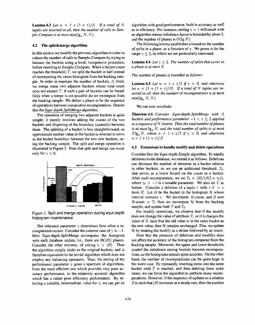
The operation of merging two adjacent buckets is quite simple; it merely involves adding the counts of the two buckets and disposing of the boundary (quantile) between them. The splitting of a bucket is less straightforward; an approximate median value in the bucket is selected to serve as the bucket boundary between the two new buckets, using the backing sample. The split and merge operation is illustrated in Figure 2. Note that split and merge can occur only for 7 > 0.

AITRIBVTI: v*t.uEF MEAN

Figure 2: Split and merge operation during equi-depth histogram maintenance

The tolerance parameter 7 determines how often a recomputation occurs. Consider the extreme case of 7 R - 1. Here Equi-depthSplitMerge recomputes the histogram with each database update, i.e., there are O(lRI) phases. Consider the other extreme, of setting 7 > (RI. Then the algorithm simply sticks to the original buckets, and is therefore equivalent to the trivial algorithm which does not employ any balancing operation. Thus, the setting of the performance parameter 7 gives a spectrum of algorithms, from the most efficient one which provides very poor accuracy performance, to the relatively accurate algorithm which has a rather poor efficiency performance. By se- lecting a suitable, intermediate, value for 7, we can get an

algorithm with good performance, both in accuracy as well as in efficiency, For instance, setting 7 = 1 will result with an algorithm whose imbalance factor is bounded by about 3, and the number of phases is O(lg N).

The following lemma establishes a bound on the number of splits in a phase, as a function of 7. We prove it for the range 7 5 2, in which we are particularly interested.

Lemma 4.4 Let 7 < 2. The number of splits that occur in a phase is at most /3.

The number of phases is bounded as follows:

Lemma 4.5 Let (Y = 1 + y/2 if 7 > 0, and otherwise let IY = (1 + (1 + 7)/j?). If a total of N tuples are inserted in all, then the number of recomputations is at most min(lg, N, N).

We can now conclude:

Theorem 4.6 Consider Equi-depthSplitMerge with p buckets and performance parameter - 1 < 7 5 2 applied to a sequence of N inserts. Then the total number of phases is at most Ig, N, and the total number of splits is at most p Ig, N, where cy = 1 + y/2 if 7 > 0, and otherwise (Y = 1 -I- (1 + 7)/P.

4.3 Extensions to handle modify and delete operations

Consider first the Equi-depthsimple algorithm. To handle deletions to the database, we extend it as follows. Deletions can decrease the number of elements in a bucket relative to other buckets, so we use an additional threshold, Te, that serves as a lower bound on the count in a bucket. After each recomputation, we set Te = IRI/(P(2 + 7e)), where 7e > - 1 is a tunable parameter. We also set T as before. Consider a deletion of a tuple r with r.X = v from R. Let B be the bucket in the histogram 7-1 whose interval contains v. We decrement Bcount, and if now Bcount = Te then we recompute fi from the backing sample, and update both T and Te.

For modify operations, we observe that if the modify does not change the value of attribute X, or if it changes the value of X such that the old value is in the same bucket as the new value, then 3-1 remains unchanged. Else, we update 31 by treating the modify as a delete followed by an insert.

Note that the presence of deletions and modifys does not affect the accuracy of the histogram computed from the backing sample. Moreover, the upper and lower thresholds control the imbalance among buckets between recomputations, so the histograms remain quite accurate. On the other hand, the number of recomputations can be quite large in the worst case. By repeatedly inserting items into the same bucket until T is reached, and then deleting these same items, we can force the algorithm to perform many recomputations. However, if the sequence of updates to a relation R is such that (RI increases at a steady rate, then the number

470

of recomputes can be bounded by a constant factor times the bound given in Lemma 4.3, where the constant depends on the rate of increase.

Now consider the Equi-depthSplitMerge algorithm. The extensions to handle delete operations are identical to those outlined above, with the following additions to handle the split and merge operations. If B.count = Te, we merge B with one of its adjacent buckets and then split the bucket B’ with the largest count, as long as B’.count 2 2(T” + 1). (Note that B’ may, or may not be the newly merged bucket.) If no such B’ exists, then we recompute 3t from the backing sample. Modify operations are handled as outlined above.

5 Fast maintenance of approximate Com- pressed histograms

In this section, we consider another important histogram type, the Compressed(V, F) histogram. We first present a “split&merge” algorithm for maintaining a Compressed histogram in the presence of database insertions, and then show how to extend the algorithm to handle database modifys and deletes. We assume throughout that a backing sample is being maintained.

Definitions. Consider a relation of (a priori unknown) size N. In an equi-depth histogram, values with high frequencies can span a number of buckets; this is a waste of buckets since the sequence of spanned buckets for a value can be replaced with a single bucket with a single count. A Com- pressed histogram has a set of such singleton buckets and an equi-depth histogram over values not in singleton buckets. Our target Compressed histogram with /3 buckets has p’ equi-depth buckets and p - p’ singleton “high-biased” buckets, where I 5 p’ 5 p, such that the following requirements hold: (Rl) each equi-depth bucket has [N’/p’J or [N’//3’1 tuples, where N’ is the total number of tuples in equi-depth buckets, (R2) no single value “spans” an equi- depth bucket, i.e., the set of bucket boundaries are distinct, and conversely, (R3) the value in each singleton bucket has frequency 2 N///3’. Associated with each bucket B is a maximum value B.maxval (either the singleton value or the bucket boundary) and a count, B.count.

An approximate Compressed histogram approximates the exact histogram by relaxing one or more of the three requirements above and/or the accuracy of the counts.

Class error metrics. Consider an approximate Com- pressed histogram ‘If with equi-depth buckets BI , . . . , Bpl and singleton buckets Bp~+l , . . . , Bp. Recall that f~ is defined to be the number of tuples in a bucket B. Let N’ be the number of tuples in equi-depth buckets, i.e., N’ = & f~,. We define two class error metrics, fled and phb (,&d is as defined in Section 4 but applied only to

the equi-depth buckets):

where U is the set of values that violate requirement (R2) or (R3). This metric penalizes for mistakes in the choice of high-biased buckets in proportion to how much the true frequencies deviate from the target threshold, N//P’, normalized with respect to this threshold.

5.1 A split&merge algorithm for Compressed histograms

We show how Equi-depthSplitMerge can be extended to handle Compressed histograms. We denote this algorithm the Compressed-SplitMerge algorithm.

On an insert of a tuple with value v into the relation, the (singleton or equi-depth) bucket, B, for ZI is determined, and the count is incremented. If B is an equi-depth bucket, then as in Equi-depthSplitMerge, we check to see if its count now equals the threshold T for splitting a bucket, and if it does, we update the bucket boundaries. The steps for updating the Compressed histogram are similar to those in Equi-depthSplitMerge, but must address several additional concerns:

1.

2.

3.

4.

New values added to the relation may be skewed, so that values that did not warrant singleton buckets before may now belong in singleton buckets.

The threshold for singleton buckets grows with N’, the number of tuples in equi-depth buckets. Thus values rightfully in singleton buckets for smaller N’ may no longer belong in singleton buckets as N’ increases.

Because of concerns 1 and 2 above, the number of equi-depth buckets, p’, grows and shrinks, and hence we must adjust the equi-depth buckets accordingly.

Likewise, the number of tuples in equi-depth buckets grows and shrinks dramatically as sets of tuples are re- moved from and added to singleton buckets. The ideal is to maintain N’/fl tuples per equi-depth bucket, but both N’ and p’ are growing and shrinking.

Our algorithm addresses each of these four concerns as follows. To address concern 1, we use the fact that a large number of updates to the same value u will suitably increase the count of the equi-depth bucket containing v so as to cause a bucket split. Whenever a bucket is split, if doing so creates adjacent bucket boundaries with the same value v, then we know to create a new singleton bucket for v. To address concern 2, we allow singleton buckets with relatively small counts to be merged back into the equi-depth

471

buckets. As for concerns 3 and 4, we use our procedures for splitting and merging buckets to grow and shrink the number of buckets, while maintaining approximate equi-depth buckets, until we recompute the histogram. The imbalance between the equi-depth buckets is controlled by the thresholds T and Te (which depend on the tunable performance parameters y and yl, as in Equi-depthSplitMerge). When we convert an equi-depth bucket into a singleton bucket or vice-versa, we ensure that at the time, the bucket is within a constant factor of the average number of tuples in an equi- depth bucket (sometimes additional splits and merges are required). Thus the average is roughly maintained as such equi-depth buckets are added or subtracted.

The requirements for when a bucket can be split or when two buckets can be merged are more involved than in Equi- depthSplitMerge: A bucket B is a candidate split bucket if it is an equi-depth bucket with B.count 2 2(Te + 1) or a singleton bucket such that T/(2 + y) 2 Bcount 2 2(Tl+ 1). A pair of buckets, Bi and Bj , is a candidate merge pair if (1) either they are adjacent equi-depth buckets or they are a singleton bucket and the equi-depth bucket in which its singleton value belongs, and (2) Bi .count + Bj .count < T. When there are more than one candidate split bucket (candidate merge pair), the algorithm selects the one with the largest (smallest combined, resp.) bucket count.

Due to space limitations, the exact details of this algorithm are presented in [3], including the procedure for computing an approximate Compressed histogram from the backing sample.

Lemma 5.1 Algorithm CompressedSplitMerge maintains the following invariants. (1) For all buckets B, B .count > Te. (2) For all equi-depth buckets B, B.count < T. (3) All bucket boundaries (B.maxval) are distinct. (4) Any value v belongs to either one singleton bucket, one equi-depth bucket or two adjacent equi-depth buckets (in the latter case, any subsequent inserts or deletes are targeted to the first of the two adjacent buckets).

Thus the set of equi-depth buckets have counts that are within a factor of T/T!, which is a small constant independent of JR] (details in the full paper).

5.2 Extensions to handle modify and delete operations

We now discuss how to extend CompressedSplitMerge to handle deletions to the database. Deletions can decrease the number of tuples in a bucket relative to other buckets, resulting in a singleton bucket that should be converted to an equi-depth bucket or vice-versa. A deletion can also drop a bucket count to the lower threshold Te.

Consider a deletion of a tuple r with T.X = v from R. Let B be the bucket in the histogram ‘H whose interval contains V. First, we decrement B.count. If B.count = Te, we do the following. If B is part of some candidate merge pair, we merge the pair with the smallest combined count

and then split the candidate split bucket B’ with the largest count. (Note that B’ may, or may not be the newly merged bucket.) If no such B’ exists, then we recompute 3-1 from the backing sample. Likewise, if B is not part of some candidate merge pair, we recompute ‘H from the backing sample. As in the insertion-only case, the conversion of buckets from singleton to equi-depth and vice-versa is pri- marily handled by detecting the need for such conversions when splitting or merging buckets.

For modify operations, we observe as before that if the modify does not change the value of attribute A, or it changes the value of A such that the old value is in the same bucket as the new value, then ‘H remains unchanged. Else, we update ‘H by treating the modify as a delete followed by an insert.

The invariants in Lemma 5.1 hold for the version of the algorithm that incorporates these extensions for modify and delete operations.

6 Experimental evaluation In this section, we experimentally study the effectiveness of our histogram-maintenance techniques and their efficiency. First, we describe the experiment testbed.

Database. We model the base data already in the database and the update data independent of each other using an extensive set of Zipf-ian [ 1 l] data distributions. The Zipf distribution was chosen because it supposedly models the skew in many real-life data quite closely. The z value was varied from 0 to 4 to vary the skew (z = 0 corresponds to the uniform distribution). The number of tuples (T) in the relation was 1OOK to start with and the number of distinct values (D) was varied from 200 to 1000. Since the exact attribute values do not affect the relative quality of our techniques, we chose the integer value domain. Finally, the frequencies were mapped to the values in different orders - decreasing (deer), increasing (incr), and random (random) -thereby generating a large collection of data distributions. We refer to a Zipf distribution with the parameter z and order z as the zipf( r , x) distribution.

Histograms. The equi-depth and Compressed histograms consisted of 20 buckets and were computed from a sample of 2000 tuples, which was also the size of the backing sample.

Updates. We used three classes of updates, described below, based on the mix of inserts, deletes, and modifys. In each case, the update data was taken from a Zipf distribution. By varying the z parameter, we can vary the skew in the updates. The number of updates was increased up to 40011’ (four times the relation size).

1. Insert: The first class of updates consists of just insert operations, Since our algorithms are most efficient for such an environment, they are studied in most detail.

472

Warehouse: This class contains an alternating sequence of a set of inserts followed by a set of deletes. This pattern is common in data warehouses keeping transactional information during sliding time windows (loading fresh data and discarding very old data, when loaded close to capacity).

Mixed: This class contains a uniform mixture of inserts, deletes, and modifys occurring in random order.

In this paper, we only present the results for the Insert class. The results for the remaining classes are given in [3].

Techniques. We studied several variants of old and new techniques which are described below in terms of their operations for a single insert (operations for delete are similar in principle).

1.

2.

3.

4.

5.

Fixed-Histogram: The sum ‘of frequencies in each bucket is incremented by i so that the total sum of the frequencies increases by 1. This is essentially the technique currently in use in nearly all systems, which treat insertions of all values the same and simply keep track of the number of tuples.

Periodic-Sample-Compute: This (expensive) technique requires recomputing the histogram from the backing sample after each insertion into the sample, while the total sum of frequencies is incremented as in the above technique.

SplitMerge: This is the class of techniques correspond- ing to the algorithms proposed in this paper.

No-Recompute: This technique differs from Split- Merge by not performing the recomputations and simply increasing the split threshold when a merge can not be performed.

Fixed-Buckets: This technique differs from Split- Merge by not attempting to split any bucket. But, unlike the Fixed-Histogram algorithm, the size of the bucket containing the inserted value is correctly incremented.

Error metrics. The following error metrics are used: pcount (Es. I), ped (Eq. 2 and 31, and PM 0% 4). In addition a new metric P,.,,~~ is defined, which captures the accuracy of histograms in estimating the result sizes of range predicates (of the form X 5 a). The query-set contains range predicates over all possible values in the joint value domain. For each query, we find the error as a percentage of the result size. P,.~,,~~ is defined as the average of these errors over the query-set.

6.1 Effects of recomputation and y

Figure 3 depicts the errors (,~,d) of the equi-depth histogram obtained at the end of 40011’ insertions as a function of y, under the SplitMerge and No-Recompute techniques. The base data distribution for this case was uniform and the update distribution was zipf(2,decr). It is clear that SplitMerge outperforms the technique without recomputations. Also, the errors due to the techniques are lowest for low values of y and increase rapidly as y increases. This is because, for low values of y the histogram is recomputed more often and the bucket sizes do not exceed a low threshold, thus keeping the p& small.

On the other hand, small values of y result in a larger number of disk accesses (for the backing sample). Figure 4 shows the effect of y on the number of recomputations. It is clear that too small values of y result in a large number of recomputations. Based on similar sets of experiments conducted over the entire set of data distributions, we con- cluded that y = 0.5 is a reasonable value for limiting the number of computations as well as for decreasing errors; we use this setting in all the remaining experiments.

6.2 Update sampling

Nearly all the experiments in this paper were conducted by considering every insertion in the database. In some update-intensive databases this could result in intolerable performance degradation. Hence we propose uniformly sampling the updates with a certain probability and mod- ifying the histograms only for the sampled updates. In this experiment, we study the effect of the update sampling probability on histogram performance. The base and update distributions are chosen to be zipf((l,incr) and zipf(0.5, random) respectively, and the histogram is Compressed. Figure 5 depicts the errors due to the SplitMerge technique for various sampling probabilities. The x-axis represents the average number of updates that are skipped and the y-axis represents the errors incurred by the histogram resulting at the end of 40011 inputs in estimating the result sizes of range queries &range). It is clear from this figure that the accuracy depends on the number of updates sampled; as long as not too many updates are skipped (say, at most 100 in this experiment), the errors are reasonably small.

6.3 Approximation of equi-depth histograms

We compare the effectiveness of various techniques in approximating equi-depth histograms under insertions into the database. The results are presented for uniform base data and zipf(2,incr) update data and are fairly consistent over most other combinations. Figures 6 through 8 contain various error measures on the y-axes, and the number of insertions on the x-axes. For this experiment, the Split- Merge technique performed just 2 recomputations while Periodic-Sample-Compute performed 3276.

473

0.x -

-Without Recomputes

0.6 - -With Recomputes

B

2’ CM-

Gamma

Figure 3: Effect of y and recomputation on &d errors

..-....‘. Fixed-Histogram ..-....‘. Fixed-Histogram - L- - Fixed-Buckets - L- - Fixed-Buckets - Periodic-Sample-Camp. - Periodic-Sample-Camp. ----- SplitMerge ----- SplitMerge

Figure 6: &,j errors (equi-depth histograms)

Figure 4: Effect of y on the number of recomputations

-+ Fixed-Buckets - Periodic-Sample-Camp. ---. SplitMerge

Figure 7: peoUnt errors (equi- depth histograms)

It is clear from Figure 6 that the SplitMerge technique is nearly identical to the more expensive Periodic-Sample- Compute technique in maintaining the histogram close to equi-depth. The Periodic-Sample-Compute technique does not maintain a perfectly equi-depth histogram because it is recomputed from the backing sample which may not reflect all the insertions. The other two techniques clearly result in a very poor equi-depth histogram because they do not perform any splits of the over-populated buckets. Figure 7 shows that the SplitMerge and Fixed-Buckets techniques are very accurate in reflecting the accurate counts, because their bucket sizes are correctly updated after every insertion. For the other two techniques, the size of a bucket is always equal to N//3, hence the p,,,nt and &d measures are identical. Finally, it is clear from Figure 8 that the SplitMerge technique offers the best performance in estimating range query result sizes as well.

6.4 Approximation of Compressed histograms

We compare the effectiveness of various techniques in maintaining approximating Compressed histograms. The base data distribution is zipf(l,incr) (a skewed distribution was chosen so that the Compressed histogram will contain a few high-biased buckets) and the update distribution is zipf(2,random), which introduces skew at different points in the relation’s distribution. Figures 9 and 10 depict the phb and p,.ange errors on the y-axes respectively and the

update samplln# Period

Figure 5: Effect of update sampling

....-. Fixed-Histogram “..-. Fixed-Histogram -.- Fixed-Buckets -.- Fixed-Buckets - Periodic-Sample-Comp. - Periodic-Sample-Comp. --- SplitMerge --- SplitMerge

jb 0 ” twmo ?.m ?Jtth ‘4mxY)

Number of Updates

Figure 8: pfange errors (equi- depth histograms)

number of insertions on the x-axes. The results for the other two metrics are similar to the equi-depth case and consistently demonstrate the accuracy of the SplitMerge technique, hence are not presented. Once again, the Split- Merge technique performed just 2 recomputations from the sample, while Periodic-Sample-Compute performed 3274 recomputations.

It can be seen from Figure 9 that the Periodic-Sample- Compute and SplitMerge techniques result in almost zero errors in capturing the high frequency values in the updated relation, even when these values were not frequent in the base relation. In the beginning, the updates do not create a new high frequency value and all techniques perform well. But once a new value becomes frequent, it is clear that the other two techniques fail to characterize it as such and hence incur high errors.

Figure 10 shows that the errors in range size estimation follow the similar pattern as the equi-depth case. Also, as expected from our earlier work [8], the Compressed histograms are observed to incur smaller errors than the equi-depth histograms from Figure 8.

6.5 Effect of skew in the updates

High skews in the update data can vary the distribution of the base relation data drastically and hence require effective histogram maintenance techniques. In Figure 11 we depict the performance of various Compressed histograms

474

..-- Fixed-Histogram a Fixed-Buckets

- Periodic-Sample-Camp. - *- SplitMerge

I, ,,MXlX, 2cmm Jcixm Number of Updales

Figure 10: P,.,,~~ errors (Com- pressed histograms)

-+ Fixed-Histogram -+ Fixed-Histogram -+-Fixed-Buckets -+-Fixed-Buckets + Periodic-Sample-Camp. + Periodic-Sample-Camp. - *- SplitMerge - *- SplitMerge

Figure 11: Effect of skew in the updates

Figure 9: phb errors (Compressed histograms)

resulting from the techniques at the end of 400K insertions to the database. ‘The x-axis contains the z parameter values and the y-axis contains the errors in estimating range query result sizes (pvange ). The Fixed-Histogram technique fails very quickly because it assumes that the updates are uniform and hence does not update the high-biased part correctly. It is clear from this figure that the SplitMerge technique performs consistently well for all levels of skew and is always better than the other techniques, because it approximates the equi-depth part well using splits and recomputations, and approximates the high-biased part well by dynamically detecting high-frequency values.

7 Conclusions

This paper proposed a novel approach for maintaining histograms and samples up-to-date in the presence of updates to the database. Algorithms were proposed for the widely used equi-depth histograms and the highly accurate class of Compressed(V,F) histograms using the novel notions of split and merge techniques and backing samples. The CPU, I/O and storage requirements for these techniques are negli- gible for insert-mostly databases and for data warehousing environments. Based on our analytical and experimental studies, our conclusions are as follows:

l The new techniques are very effective in approximating equi-depth and Compressed histograms. They are equally effective for relations orders of magnitude larger. In fact, as the relation size grows, the relative overhead of maintaining the backing sample necessary for the same performance, becomes even smaller.

l Very few recomputations from the backing sample are incurred for a large number of updates, proving that our split&merge techniques are quite effective in min- imizing the overheads due to recomputation.

l The experiments clearly show that histograms maintained using these techniques remain highly effective in result size estimation, unlike the current approaches.

Based on our results, we recommend that these techniques be used in most DBMSs, for effective incremental maintenance of approximate histograms.

Acknowledgments. We acknowledge the contributions of Andy Wrtkowski to the algorithm for maintaining approximate equi-depth histograms. We also thank Nabil Kahale and Sridhar Rajagopalan for discussions related to this work.

References [l] S. Christodoulakis. Implications of certain assumptions in

database performance evaluation. ACM TODS, 9(2): 163- 186, June 1984.

[2] P B. Gibbons and Y. Matias. Space-efficient maintenance of top sellers lists in large databases. Manuscript., July 1996.

[3] P. B. Gibbons, Y. Matias, and V. Poosala. Fast incremental maintenance of approximate histograms. Technical report, Bell Laboratories, Murray Hill, NJ, June 1997.

[4] Y. Ioannidis and S. Christodoulakis. On the propagation of errors in the size of join results. Proc. of ACM SIGMOD Co& pages 268-277,199 1.

[5] R. P. Kooi. The optimization of queries in relational databases. PhD thesis, Case Western Reserver University, Sept. 1980.

[6] V. Poosala. Histogram-based estimation techniques in database systems. PhD thesis, Univ. of Wisconsin-Madison, Feb. 1997.

[7] V. Poosala and Y. Ioannidis. Estimation of query-result distribution and its application in parallel-join load balancing. Proc. of the 22nd Int. Conf on Very Large Databases, pages 448459, Sept. 1996.

(81 V. Poosala, Y. Ioannidis, P. Haas, and E. Shekita. Improved histograms for selectivity estimation of range predicates. Proc. of ACM SIGMOD ConJ pages 294-305, June 1996.

[9] P. Selinger, M. Astrahan, D. Chamberlin, R. Lorie, and T. Price. Access path selection in a relational database man- agement system. Proc. ofACMSIGMOD Conf, pages 23-34, 1979.

[ 101 J. S. Vitter. Random sampling with a reservoir. ACM Trans. Math. Softiare, 11:37-57, 1985.

[l l] G. K. Zipf. Human behaviour and the principle of least e$ort. Addison-Wesley, Reading, MA, 1949.

475

fast incremental maintenance of approximate histograms · fast incremental maintenance of...

Documents