fast generalized subset scan for anomalous pattern detection
TRANSCRIPT

Journal of Machine Learning Research 14 (2013) 1533-1561 Submitted 4/12; Revised 1/13; Published 6/13
Fast Generalized Subset Scan for Anomalous Pattern Detection
Edward McFowland III [email protected]
Skyler Speakman [email protected]
Daniel B. Neill [email protected]
Event and Pattern Detection Laboratory
H.J. Heinz III College
Carnegie Mellon University
Pittsburgh, PA 15213 USA
Editor: Tony Jebara
Abstract
We propose Fast Generalized Subset Scan (FGSS), a new method for detecting anomalous patterns
in general categorical data sets. We frame the pattern detection problem as a search over subsets
of data records and attributes, maximizing a nonparametric scan statistic over all such subsets.
We prove that the nonparametric scan statistics possess a novel property that allows for efficient
optimization over the exponentially many subsets of the data without an exhaustive search, enabling
FGSS to scale to massive and high-dimensional data sets. We evaluate the performance of FGSS
in three real-world application domains (customs monitoring, disease surveillance, and network
intrusion detection), and demonstrate that FGSS can successfully detect and characterize relevant
patterns in each domain. As compared to three other recently proposed detection algorithms, FGSS
substantially decreased run time and improved detection power for massive multivariate data sets.
Keywords: pattern detection, anomaly detection, knowledge discovery, Bayesian networks, scan
statistics
1. Introduction
We focus on the task of detecting anomalous patterns in massive, multivariate data sets. The anoma-
lous pattern detection task arises in many domains: customs monitoring, where we attempt to dis-
cover patterns of illicit container shipments; disease surveillance, where we must detect emerging
outbreaks of disease in the very early stages; network intrusion detection, where we attempt to
identify patterns of suspicious network activities; and various others. The underlying assumption of
anomalous pattern detection is that the majority of the data is generated according to the same distri-
bution representing the (typically unknown and possibly complex) normal behavior of the system,
and thus we wish to detect groups of records which are unexpected given the typical data distri-
bution. Most existing anomaly detection methods focus on the discovery of single anomalous data
records, for example, detecting a fraudulent transaction in financial data. However, an intelligent
fraudster will attempt to disguise their activity so that it closely resembles legitimate transactions.
In such a case, each individual fraudulent transaction may only be slightly anomalous, and thus it is
only by detecting groups of such transactions that we can discover the pattern of fraud.
Alternatively, customs officials who are tasked with detecting smuggling efforts must decide
which of the many containers entering the country daily should be opened for inspection. If a
smuggler has discovered an effective method for concealing contraband, he may make similar il-
c©2013 Edward McFowland III, Skyler Speakman and Daniel B. Neill.

MCFOWLAND III, SPEAKMAN AND NEILL
licit shipments—for example, through the same shipping company, to the same port, and/or with
the same declared contents—in the future. By searching for groups of these similar and slightly
anomalous shipments, we can detect the presence of the subtle underlying pattern of smuggling. As
a concrete example, in §4.1 we analyze a data set of real-world container shipments, with attributes
including country of origin, commodity, size, weight, and value. Our approach, described in §2,
can identify self-similar subsets of data records (container shipments) for which any subset of these
attributes are anomalous, for example, shipments of pineapple from the same country, each with
elevated weights as a result of the fruits being hollowed out and filled with drugs. Similarly, in the
disease surveillance domain, health officials may wish to ignore a single hospital Emergency De-
partment (ED) having an increased number of patient visits. This could be due to noise or associated
with a completely different process that does not reflect an actual disease outbreak. However, health
officials are very interested when a group of hospital locations, perhaps within a close proximity
to each other, all have an increase in the number of ED visits. As a concrete example, in §4.2 we
analyze a data set of real-world Emergency Department visits from Allegheny County, PA, with
attributes including hospital id, prodrome, age decile, gender, and zip code. Our approach can iden-
tify subsets of data records (ED visits) for which any subset of attributes are anomalous, enabling
early and accurate outbreak detection.
1.1 The Anomalous Pattern Detection Problem
Here we focus on the problem of anomalous pattern detection in general data, that is, data sets
where data records are described by an arbitrary set of attributes. We describe the anomalous pat-
tern detection problem as detecting groups of anomalous records and characterizing their anomalous
features, with the intention of understanding the anomalous process that generated these groups.
The anomalous pattern detection task begins with the assumption that there are a set of processes
generating records in a data set. The “background” process generates records that are typical and
expected; these records are assumed to constitute the majority of the data set. Records that do not
correspond to the background data pattern, and therefore represent atypical system behavior, are
assumed to have been generated by an anomalous process and follow an alternative data pattern. If
these anomalies are generated by a process which is very different from the background process,
it may be sufficient to evaluate each individual record in isolation because many of the records’
attributes will be atypical, or individual attributes may take on extremely surprising values. How-
ever, a subtle anomalous process will generate records that may each be only slightly anomalous
and therefore extremely challenging to detect. The key insight is to acknowledge and leverage the
group structure of these records, since we expect records generated by the same process to have a
high degree of similarity. Therefore, we propose to detect self-similar groups of records, for which
some subset of attributes are unexpected given the background data distribution.
While searching over groups of records (rather than individual records) may substantially in-
crease detection power, performing this search for general data sets presents several challenges.
Many previously proposed pattern detection methods are optimized to detect patterns in data from
a specific domain, such as fraud detection or disease surveillance, but cannot be as easily applied to
other domains (Chau et al., 2006; Neill and Cooper, 2010; Neill, 2011). Typically these methods can
attribute their success to prior knowledge of the behavior of relevant patterns of anomalies. Con-
versely, general methods for anomalous pattern detection are most useful for identifying interesting
and non-obvious patterns occurring in the data, when there is little knowledge of what patterns to
1534

FAST GENERALIZED SUBSET SCAN FOR ANOMALOUS PATTERN DETECTION
look for. All of the pattern detection methods considered in this work use background data to learn
a null model M0, where M0 captures the joint probability distribution over the set of attributes under
the null hypothesis H0 that nothing of interest is occurring. A general anomalous pattern detection
method must learn M0 while making few assumptions, as it must maintain the ability to detect pre-
viously unknown and relevant patterns across diverse data without prior knowledge of the domain
or the true distribution from which the data records are drawn.
We can reduce the challenge of anomalous pattern detection in general data to a sequence of
tasks: learning a null model, defining the search space (i.e., which subsets of the data will be
considered), choosing a function to score the interestingness or anomalousness of a subset, and
optimizing this function over the search space in order to find the highest scoring subsets. There-
fore, we briefly summarize several previously proposed methods for anomalous pattern detection in
general categorical data sets based on their techniques, and their limitations, for addressing these
tasks; more detailed descriptions can be found in §3. Each method discussed here, including our
proposed Fast Generalized Subset Scan approach, learns the structure and parameters of a Bayesian
network from training data to represent M0, and then searches for subsets of records in test data
that are collectively anomalous given M0. The training data can be historical data, background data,
or simply a separate data set. However, the methods do assume that the training data set does not
contain anomalous patterns. Das and Schneider (2007) present a simple solution to the problem of
individual record anomaly detection by computing each record’s likelihood given M0, and assuming
that the lowest-likelihood records are most anomalous; we refer to this approach as the Bayesian
Network Anomaly Detector (BN). Although BN is able to locate highly individually anomalous
records very quickly, it will lose power to detect anomalous groups produced by a subtle anomalous
process where each record, when considered individually, is only slightly anomalous. Furthermore,
BN ignores the group structure of anomalies and thus fails to provide specific details (groups of
records, or subsets of attributes for which these records are anomalous) useful for understanding the
underlying anomalous processes. Anomaly Pattern Detection (APD) first computes each record’s
likelihood given M0, assuming that the lowest-likelihood records are individually anomalous, and
then finds rules (conjunctions of attribute values) with higher than expected numbers of individu-
ally anomalous records (Das et al., 2008). APD improves on BN by allowing for subsets larger
than one record. However, like BN, APD loses power to detect subtle anomalies because of its de-
pendency on individual record anomalousness. Also, APD permits records within a group to each
be anomalous for different reasons, therefore compromising its ability to differentiate between true
examples of anomalous patterns and noise, and making it difficult to characterize why a given sub-
set is anomalous. Anomalous Group Detection (AGD) maximizes a likelihood ratio statistic over
subsets of records, where a subset’s likelihood under H0 is computed from the null model Bayesian
network and the subset’s likelihood under H1 is computed from a Bayesian network learned specif-
ically from the subset of interest (Neill et al., 2008; Das, 2009). The search spaces of all possible
rules and all possible subsets are too vast to search over exhaustively for APD and AGD respec-
tively. Therefore both approaches reduce their search spaces, by using a set of 2-component rules
for APD and a greedy heuristic search for AGD. In both cases, the algorithm may fail to identify the
most interesting subset of the data. Therefore the current state of the literature requires anomalies to
be found either in isolation or through a reduction in the search space, when searching for groups,
which could remove the anomalous groups of interest from consideration. In §2 we propose an
algorithm, Fast Generalized Subset Scan (FGSS), that can efficiently maximize a scoring function
over all possible subsets of data records and attributes, allowing us to find the most anomalous sub-
1535

MCFOWLAND III, SPEAKMAN AND NEILL
set. Furthermore, our algorithm does not depend on the anomalousness of an entire record, but only
some subset of its attributes, and is therefore able to provide useful information about the underlying
anomalous process by identifying the subset of attributes for which a group is anomalous.
2. Fast Generalized Subset Scan
Fast Generalized Subset Scan (FGSS) is a novel method for anomalous pattern detection in general
categorical data. Unlike previous methods, we frame the pattern detection problem as a search
over subsets of data records and subsets of attributes; we therefore search for self-similar groups of
records for which some subset of attributes is anomalous. More precisely, we define a set of data
records R1 . . .RN and attributes A1 . . .AM. Here we assume that all attributes are categorical, but
future work will extend the approach to continuous attributes as well. For each record Ri, we assume
that we have a value vi j for each attribute A j. We then define the subsets S under consideration to be
S = R×A, where R⊆ {R1 . . .RN} and A⊆ {A1 . . .AM}. We wish to find the most anomalous subset
S∗ = R∗×A∗ = argmaxS
F(S),
where the score function F(S) defines the anomalousness of a subset of records and attributes. We
accomplish this by first learning a Bayesian network model, M0, from the training data. For each
value vi j (the value of attribute A j for record Ri), FGSS then computes its likelihood li j given M0.
This likelihood represents the conditional probability of the observed value vi j under the null hy-
pothesis H0, given its parent attribute values for record Ri. Then the method computes an empirical
p-value range pi j for each li j, which serves as a measure of how uncommon it is to see a likelihood
as low as li j under H0. More specifically, pi j is computed by ranking the likelihoods li j for a given
attribute A j, with the rankings then scaled to [0,1]. Finally, FGSS searches for subsets that contain
an unexpectedly large number of low (significant) empirical p-value ranges, as such a subset is more
likely to have been generated by an anomalous process.
2.1 Learning the Data Probability Distribution
The FGSS algorithm first learns a Bayesian network which models the probability distribution of
the data under the assumption of the null hypothesis that no anomalous patterns exist. As in the
previously proposed BN, APD, and AGD methods, this Bayesian network is typically learned from
a separate “clean” data set of training data assumed to contain no anomalous patterns, but can
also be learned from the test data if the proportion of anomalies is assumed to be very small. We
use the Optimal Reinsertion algorithm proposed by Moore and Wong (2003) to learn the structure
of the Bayesian network, using smoothed maximum likelihoods to estimate the parameters of the
conditional probability table. Smoothing provides a means to handle sparsity of the training data,
as it is possible that combinations of attribute values which appear in the test data will not appear
in the training data. In such cases we would like to assume a low, but non-zero, probability for the
corresponding entries in the conditional probability table.
If we consider the node corresponding to attribute A j in our Bayesian network M0 and let Ap( j)
represent its parent nodes, then we represent the parameters of the conditional probability tables as
follows:
θ jmk = PM0(A j = m |Ap( j) = k) ∀ j,m,k.
1536

FAST GENERALIZED SUBSET SCAN FOR ANOMALOUS PATTERN DETECTION
To estimate θ jmk, let N jmk correspond to the number of instances in the data where A j = m and
Ap( j) = k. To apply Laplace smoothing, we define the arity of A j as C and add 1/C to each N jmk.
Therefore, our smoothed parameter estimates are computed as
θ̂ jmk =N jmk +1/C
∑m′(N jm′k +1/C),
thus assuming that the total weight of the prior sums to one for each attribute A j and set of parent
values Ap( j). After learning a model of the data distribution under the null hypothesis, FGSS then
computes
li j = PM0(A j = vi j |Ap( j) = vi,p( j)),
representing the individual attribute-value likelihoods of each attribute for a given record, condi-
tioned on its parent attribute values for that record. We compute these individual attribute-value
likelihoods for all records in the training and test data sets.
2.2 Computing Empirical p-value Ranges
The calculation of empirical p-value ranges in the test data set requires obtaining a ranking of the
likelihoods li j for each attribute A j. To do so, we calculate for each likelihood li j the quantities
Nbeat(li j) = ∑Rk∈Dtrain
I(lk j < li j),
Ntie(li j) = ∑Rk∈Dtrain
I(lk j = li j).
We then define the empirical p-value range corresponding to likelihood li j as
pi j = [pmin(pi j), pmax(pi j)]
=
[
Nbeat(li j)
Ntrain +1,Nbeat(li j)+Ntie(li j)+1
Ntrain +1
]
,(1)
where Ntrain is the total number of training data records.
To properly interpret the concept of an empirical p-value range, we first consider the traditional
empirical p-value
p̂(x) =1
n
n
∑z=1
I(Xz ≤ x)
for n data samples, which closely resembles pmax(pi j), the upper limit of pi j. For an attribute A j,
corresponding to a column in the test data set, there is some true distribution of likelihoods li j under
H0. Since the training data is assumed to contain no anomalous patterns, we can estimate the true
cumulative distribution function FL j(l) with an empirical cumulative distribution function
F̂L j(l) =
Nbeat(l)+Ntie(l)
Ntrain
derived from the training data set. Then the empirical p-value corresponding to a given likelihood li j
in the test data set can be defined as p̂(li j) = F̂L j(li j). If the null hypothesis is true, then the test data
set also has no anomalous patterns, and is generated from the same distribution as the training data
1537

MCFOWLAND III, SPEAKMAN AND NEILL
set. In this case, the empirical p-values p̂(li j) will be asymptotically distributed as Uniform[0,1] for
each attribute A j. Davison and Hinkley (1997) note that the smoothed empirical p-value
p̂(l) = F̂L j(l) =
Nbeat(l)+Ntie(l)+1
Ntrain +1
is also asymptotically unbiased, and is a more accurate estimator of the true p-value. This definition
also guards against obtaining an empirical p-value of zero, which is consistent with our knowledge
that true p-values are non-zero.
Our FGSS algorithm extends the concept of empirical p-values to empirical p-value ranges in
order to appropriately handle ties in likelihoods. In the general data set context, we often see many
records with identical attribute-value likelihoods, typically as a result of identical attribute values.
Using an empirical p-value, where tied likelihoods are treated identically to lower likelihood val-
ues, will introduce a bias toward larger p-values when ties in likelihood are present. However,
under the null hypothesis that the training and test data sets are drawn from the same distribution,
if we compute the empirical p-value ranges as defined in (1) and then draw an empirical p-value
uniformly at random from each range [pmin(pi j), pmax(pi j)], then the resulting empirical p-values
will be asymptotically distributed as Uniform[0,1]. As a concrete example, if a given attribute was
entirely uninformative (i.e., all training and test data records had identical likelihoods for that at-
tribute), we would obtain an empirical p-value range of [0,1] for each test record, while the previous
empirical p-value approach would set each empirical p-value equal to 1.
For a single p-value, p, we can define an indicator variable nα(p) representing whether or not
that p-value is significant at level α:
nα(p) = I(p≤ α).
This traditional definition of significance can be extended naturally to p-value ranges by considering
the proportion of each range that is significant at level α, or equivalently, the probability that a p-
value drawn uniformly from [pmin(pi j), pmax(pi j)] is less than α. The quantity nα(pi j) representing
the significance of a p-value range is therefore defined as:
nα(pi j) =
1 if pmax(pi j)< α
0 if pmin(pi j)> αα−pmin(pi j)
pmax(pi j)−pmin(pi j)otherwise.
For a subset S, we can then define the quantities
Nα(S) = ∑vi j∈S
nα(pi j), (2)
N(S) = ∑vi j∈S
1 (3)
where N(S) represents the total number of empirical p-value ranges contained in subset S. Nα(S)can informally be described as the number of p-value ranges in S which are significant at level α, but
is more precisely the total probability mass less than α in these p-value ranges, since it is possible
for a range pi j to have pmin(pi j) ≤ α ≤ pmax(pi j). For a subset S consisting of N(S) empirical
1538

FAST GENERALIZED SUBSET SCAN FOR ANOMALOUS PATTERN DETECTION
p-value ranges, we can compute the expected number of significant p-value ranges under the null
hypothesis H0:
E [Nα(S)] = E
[
∑vi j∈S
nα(pi j)
]
= ∑vi j∈S
E [nα(pi j)]
= ∑vi j∈S
α
= αN(S).
We note that this equation follows from the property that the empirical p-values are identically
distributed as Uniform[0,1] under the null hypothesis, and holds regardless of whether the p-values
are independent. Under the alternative hypothesis, we expect the likelihoods li j (and therefore the
corresponding p-value ranges pi j) to be lower for the affected subset of records and attributes,
resulting in a higher value of Nα(S) for some α. Therefore a subset S where Nα(S)> αN(S) (i.e., a
subset with a higher than expected number of low, significant p-value ranges) is potentially affected
by an anomalous process.
2.3 Nonparametric Scan Statistic
To determine which subsets of the data are most anomalous, FGSS uses a nonparametric scan statis-
tic (Neill and Lingwall, 2007) to compare the observed and expected number of significantly low
p-values contained in subset S. We define the general form of the nonparametric scan statistic as
F(S) = maxα
Fα(S) = maxα
φ(α,Nα(S),N(S)) (4)
where Nα(S) and N(S) are defined as in (2) and (3) respectively. We assume that the function
φ(α,Nα,N) satisfies several intuitive properties that will also allow efficient optimization:
(A1) φ is monotonically increasing w.r.t. Nα.
(A2) φ is monotonically decreasing w.r.t. N and α.
(A3) φ is convex.
These assumptions follow naturally because the ratio of observed to expected number of significant
p-values NαNα increases with the numerator (A1), and decreases with the denominator (A2). Also,
a fixed ratio of observed to expected should be more significant when the observed and expected
counts are large (A3).
We consider “significance levels” α between 0 and some constant αmax < 1. If there is a prior
expectation of the subtleness of the anomalous process, αmax can be chosen appropriately. The
less subtle the anomalous process, that is, the more individually anomalous the records it generates
are expected to be, the lower αmax can be set. We note that maximizing of F(S) over a range
of α values, rather than for a single arbitrarily-chosen value of α, enables the nonparametric scan
statistic to detect a small number of highly anomalous p-values, a larger number of subtly anomalous
p-values, or anything in between.
In this work we explore the use of two functions φ(α,Nα,N) which satisfy the monotonicity and
convexity properties (A1)-(A3) assumed above: the Higher Criticism (HC) statistic (Donoho and
1539

MCFOWLAND III, SPEAKMAN AND NEILL
Jin, 2004) and the Berk-Jones (BJ) statistic (Berk and Jones, 1979). The HC statistic is defined as
follows:
φHC(α,Nα,N) =Nα−Nα
√
Nα(1−α). (5)
Under the null hypothesis of uniformly distributed p-value ranges, and the additional simplifying
assumption of independence between p-value ranges, the number of empirical p-value ranges less
than α is binomially distributed with parameters N and α. Therefore the expected number of p-
value ranges less than α under H0 is Nα, with a standard deviation of√
Nα(1−α). This implies
that the HC statistic can be interpreted as the test statistic of a Wald test for the number of significant
p-value ranges. We note that the assumption of independent p-value ranges is not necessarily true in
practice, since our method of generating these p-value ranges may introduce dependence between
the p-values for a given record; nevertheless, this assumption results in a simple and efficiently
computable score function.
The BJ statistic is defined as:
φBJ(α,Nα,N) = NK
(
Nα
N,α
)
, (6)
where K is the Kullback-Liebler divergence,
K(x,y) = x logx
y+(1− x) log
1− x
1− y,
between the observed and expected proportions of p-values less than α. The BJ statistic can be de-
scribed as the log-likelihood ratio statistic for testing whether the empirical p-values are uniformly
distributed on [0,1], where the alternative hypothesis assumes a piecewise constant distribution with
probability density function
f (x) =
{
f1 for 0≤ x≤ α
f2 for α≤ x≤ 1
with f1 > f2.
Berk and Jones (1979) demonstrated that this test statistic fulfills several optimality properties and
has greater power than any weighted Kolmogorov statistic.
We note that the original version of the nonparametric scan statistic, used for spatial data by
Neill and Lingwall (2007), considered the HC statistic (5) only, and used empirical p-values rather
than p-value ranges. Our empirical results below demonstrate that the BJ statistic (6) outperforms
HC for some real-world anomalous pattern detection tasks, and our use of empirical p-value ranges
guarantees unbiased scores even when ties in likelihood are present. Furthermore, we present a
novel approach for efficient optimization of any nonparametric scan statistic (satisfying the mono-
tonicity and convexity properties (A1)-(A3) assumed above) over subsets of records and attributes,
as described below.
2.3.1 EFFICIENT NONPARAMETRIC SUBSET SCANNING
Although the nonparametric scan statistic provides a function F(S) to evaluate the anomalousness of
subsets in the test data, naively maximizing F(S) over all possible subsets of records and attributes
1540

FAST GENERALIZED SUBSET SCAN FOR ANOMALOUS PATTERN DETECTION
would be infeasible for even moderately sized data sets, with a computational complexity of O(2N×2M). However, Neill (2012) defined the linear-time subset scanning (LTSS) property, which allows
for efficient and exact maximization of any function satisfying LTSS over all subsets of the data. For
a pair of functions F(S) and G(Ri), which represent the “score” of a given subset S and the “priority”
of data record Ri respectively, the LTSS property guarantees that the only subsets with the potential
to be optimal are those consisting of the top-k highest priority records {R(1) . . .R(k)}, for some k
between 1 and N. This property enables us to search only N of the 2N subsets of records, while still
guaranteeing that the highest-scoring subset will be found. We demonstrate that the nonparametric
scan statistics satisfy the necessary conditions for the linear-time subset scanning property to hold,
allowing efficient maximization over subsets of data records (for a given subset of attributes) or
over subsets of attributes (for a given subset of records). In the following section, we will show how
these efficient optimization steps can be combined to enable efficient joint maximization over all
subsets of records and attributes. We begin by restating a theorem from Neill (2012):
Theorem 1 (Neill, 2012) Let F(S) = F(X , |S|) be a function of one additive sufficient statistic of
subset S, X(S) = ∑Ri∈S xi (where xi depends only on record Ri), and the cardinality of S. Assume
that F(S) is monotonically increasing with X. Then F(S) satisfies the LTSS property with priority
function G(Ri) = xi.
Corollary 2 We consider the general class of nonparametric scan statistics as defined in (4), where
the significance level α is allowed to vary from zero to some constant αmax. For a given value of
α, and assuming a given subset of attributes A⊆ {A1 . . .AM} under consideration, we demonstrate
that Fα(S) can be efficiently maximized over all subsets S = R×A, for R ⊆ {R1 . . .RN}. First, we
know that every record Ri has the same number |A| of p-value ranges, and thus N(S) ∝ |R|. Hence
we can write
Fα(S) = φ(α,Nα(R), |R|),
where the additive sufficient statistic Nα(R) is defined as follows:
Nα(R) = ∑Ri∈R
∑A j∈A
nα(pi j).
Since the nonparametric scan statistic is defined to be monotonically increasing with Nα (A1), we
know that Fα(S) satisfies the LTSS property with priority function
Gα(Ri) = ∑A j∈A
nα(pi j). (7)
Therefore the LTSS property holds for each value of α, enabling each Fα(S) to be efficiently
maximized over subsets of records. Nearly identical reasoning can be used to demonstrate that
Fα(S) can be efficiently maximized over all subsets S = R×A, for A ⊆ {A1 . . .AM}, assuming a
given set of records R⊆ {R1 . . .RN}. In this case,
Fα(S) = φ(α,Nα(A), |A|)
satisfies the LTSS property with priority function
Gα(A j) = ∑Ri∈R
nα(pi j). (8)
1541

MCFOWLAND III, SPEAKMAN AND NEILL
Thus the LTSS property enables efficient computation of maxS Fα(S) for a given value of α, but
we must still consider how to maximize this function over all values of α, for 0 < α ≤ αmax. We
demonstrate that only a small set of α levels must be examined, and therefore
maxS
F(S) = maxα
maxS
Fα(S)
can also be computed efficiently. More precisely, we demonstrate that only the maximum value
pmax(pi j) of each p-value range pi j in the subset S must be considered as a possible value of α. We
first define some preliminaries:
Definition 3 Let U(S,αmax) be the set of distinct values {pmax(pi j) : vi j ∈ S, pmax(pi j) ≤ αmax}∪{0,αmax}.
Definition 4 Let α(k) be the kth smallest value in U(S,αmax). We will consider the set of intervals
[α(k),α(k+1)], for k = 1 . . . |U(S,αmax)|−1.
Definition 5 Let P(S,α) = {pi j : vi j ∈ S,α ∈ pi j}, be the set of p-value ranges pi j in S such that
pmin(pi j)≤ α≤ pmax(pi j).
Lemma 6 Nα(S) is a convex function of α over each interval [α(k),α(k+1)], for k= 1 . . . |U(S,αmax)|−1.
Proof of Lemma 6 We consider two cases, one of which will hold for any given interval [α(k),α(k+1)].In either case, we note that no pmax values are contained within the interval, that is, for all values
vi j ∈ S and the corresponding p-value ranges pi j, pmax(pi j) /∈ (α(k),α(k+1)). We begin by observing
that∂Nα(S)
∂α= ∑
pi j∈P(S,α)
1
pmax(pi j)− pmin(pi j). (9)
Case 1: For all values vi j ∈ S and the corresponding p-value ranges pi j, pmin(pi j) /∈ (α(k),α(k+1)).In this case, no p-value range begins or ends within the interval, and thus P(S,α) is constant over
the entire interval (α(k),α(k+1)). Therefore, we know that (9) equals a positive constant over the
entire interval, and thus Nα(S) is a linear (and therefore convex) function of α.
Case 2: For some value(s) vi j ∈ S and the corresponding p-value ranges pi j, pmin(pi j)∈ (α(k),α(k+1)).As for Case 1, we know that (9) is piecewise constant, and therefore Nα(S) is a piecewise linear func-
tion of α. We note additionally that, for a given pmin(pi j), the slope described in (9) increases by1
pmax(pi j)−pmin(pi j)> 0 at α = pmin(pi j).
From these two cases, we conclude that, as a function of α, Nα(S) is piecewise linear with an
increasing slope at each value pmin(pi j), a decreasing slope at each value pmax(pi j), and an other-
wise constant slope. Therefore, within each interval defined by [α(k),α(k+1)] and thus containing no
values pmax(pi j), we know that Nα(S) is convex.
Theorem 7 If Fα(S) = φ(α,Nα(S),N(S)) satisfies assumptions (A1)-(A3) given in §2.3, then
maxα
Fα(S) = maxα∈U(S,αmax)
Fα(S).
1542

FAST GENERALIZED SUBSET SCAN FOR ANOMALOUS PATTERN DETECTION
Proof of Theorem 7 For any point αint in the open interval (α(k),α(k+1)), we show that:
Fαint(S)≤max{Fα(k)
(S),Fα(k+1)(S)}.
To see this, we can write
αint = λα(k)+(1−λ)α(k+1)
where 0 < λ < 1.
Then the proof proceeds as follows:
Fαint(S) = φ(αint,Nαint
(S),N(S))
≤ φ(αint,λNα(k)(S)+(1−λ)Nα(k+1)
(S),N(S))
≤max{Fα(k)(S),Fα(k+1)
(S)}.
The first inequality follows from the assumption (A1) that φ(α,Nα,N) is monotonically increasing
with Nα: by Lemma 6, we know that
Nαint(S)≤ λNα(k)
(S)+(1−λ)Nα(k+1)(S).
The second inequality follows from the assumption (A3) that φ(α,Nα,N) is convex.
We can conclude that, when computing maxα Fα(S), only values of α ∈ U(S,αmax) (Defini-
tion 3) must be considered, as there will not be any local maxima of the function outside of this set.
This fact, combined with Theorem 1, demonstrates that
maxS
F(S) = maxα
maxS
Fα(S)
= maxα∈U(S,αmax)
maxS
Fα(S)(10)
can be efficiently and exactly computed over all subsets S = R×A, where R ⊆ {R1 . . .RN}, for a
given subset of attributes A. To do so, we consider the set of distinct α values U =U({R1 . . .RN}×A,αmax). For each α ∈U , we employ the same logic as described in Corollary 2 to optimize Fα(S):compute the priority Gα(Ri) for each record as in (7), sort the records from highest to lowest priority,
and evaluate subsets S = {R(1) . . .R(k)}×A consisting of the top-k highest priority records, for k =1 . . .N. For each of the |U | values of α under consideration, the aggregation step requires O(N|A|) =O(NM) time, sorting the records by priority requires O(N logN) time, and evaluation of the N
subsets requires O(N) time, giving a total complexity of O(|U |N(M+ logN)) for this optimization
step. In the unconstrained case (as opposed to the similarity-constrained FGSS approach described
in §2.5), |U | tends to grow linearly with N. However, even though we must consider N|A| p-values,
we note that |U | is upper bounded by the number of distinct likelihood values li j with corresponding
pmax(pi j) ≤ αmax in the conditional probability tables of the Bayesian network learned in the first
step of the FGSS algorithm, and thus tends to be much smaller than N|A| in practice.
Similarly, (10) can be efficiently and exactly computed over all subsets S = R× A, where
A ⊆ {A1 . . .AM}, for a given subset of records R. In this case, we consider the set of distinct α
values U = U(R×{A1 . . .AM},αmax). For each α ∈ U , we again employ the same logic as de-
scribed in Corollary 2 to optimize Fα(S): compute the priority Gα(A j) for each attribute as in (8),
1543
MCFOWLAND III, SPEAKMAN AND NEILL
sort the attributes from highest to lowest priority, and evaluate subsets S = R×{A(1) . . .A(k)} con-
sisting of the top-k highest priority attributes, for k = 1 . . .M. For each of the |U | values of α under
consideration, the aggregation step requires O(M|R|) = O(MN) time, sorting the attributes by pri-
ority requires O(M logM) time, and evaluation of the M subsets requires O(M) time, giving a total
complexity of O(|U |M(N + logM)) for this optimization step.
2.4 Search Procedure
Given the two efficient optimization steps described above (optimizing over all subsets of attributes
for a given subset of records, and optimizing over all subsets of records for a given subset of at-
tributes), we propose two different search procedures for maximizing the score function F(S) over
all subsets of records and attributes. The first approach, which we call “exhaustive FGSS”, performs
an efficient search over records separately for each of the 2M subsets of attributes. This approach
is computationally efficient when the number of attributes is small, and is guaranteed to find the
globally optimal subset of records and attributes. However, its run time scales exponentially with
the number of attributes (Table 1), with a total complexity of O(2M|U |N(M+ logN)), and thus the
exhaustive FGSS approach is not feasible for data sets with a large number of attributes.
Thus we propose the FGSS search procedure that scales well with both N and M, using LTSS
to efficiently maximize over subsets of records and subsets of attributes. To do so, we first choose a
subset of attributes A ⊆ {A1...AM} uniformly at random. We then iterate between the two efficient
optimization steps described above. We first maximize F(S) over all subsets of records for the
current subset of attributes A, and set the current set of records as follows:
R = argmaxR⊆{R1...RN}F(R×A). (11)
We then maximize F(S) over all subsets of attributes for the current subset of records R, and set the
current set of attributes as follows:
A = argmaxA⊆{A1...AM}F(R×A). (12)
We continue iterating between (11) and (12) until convergence, at which point we have reached a
conditional maximum of the score function (R is conditionally optimal given A, and A is condi-
tionally optimal given R). This ordinal ascent approach is not guaranteed to converge to the joint
optimum
argmaxR⊆{R1...RN},A⊆{A1...AM}F(R×A),
but multiple random restarts can be used to approach the global optimum. We show in §4 that with
50 random restarts, FGSS will locate a near globally optimal subset with high probability. Moreover,
if N and M are both large, this iterative search is much faster than an exhaustive search approach,
making it computationally feasible to detect anomalous subsets of records and attributes in data sets
that are both large and high-dimensional. Each iteration (optimization over records, followed by
optimization over attributes) has a complexity of O(|U |(NM +N logN +M logM)), where |U | is
the average number of α thresholds considered. In this expression, the O(NM) term results from
aggregating over records and attributes, while the O(N logN) and O(M logM) terms result from
sorting the records and attributes by priority respectively. Thus the FGSS search procedure has a
total complexity of O(Y Z|U |(NM+N logN +M logM)), where Y is the number of random restarts
and Z is the average number of iterations required for convergence (Table 1). Since each iteration
1544

FAST GENERALIZED SUBSET SCAN FOR ANOMALOUS PATTERN DETECTION
Search Procedure # of StepsOptimizing Optimizing Aggregating
Records Attributes Records and Attributes
Exhaustive 2M|U | O(N logN) - O(NM)
Efficient Y Z|U | O(N logN) O(M logM) O(NM)
Exhaustive w/2M|U |N O(k logk) - O(kM)
Similarity Constraints
Efficient w/Y Z|U |N O(k logk) O(M logM) O(kM)
Similarity Constraints
Table 1: Outline of the computational complexity of each FGSS search procedure. From left to right
the columns describe: the particular search procedure, the number of optimization steps
required, the complexity of sorting over records per optimization step, the complexity
of sorting over attributes per optimization step, and the complexity of aggregating over
records and attributes per optimization step.
Variable Definitions:
|U | is the average number of α thresholds considered.
Y is the number of random restarts (efficient methods only).
Z is the average number of iterations required for convergence (efficient
methods only).
M is the number of attributes.
N is the number of records.
k is the average neighborhood size corresponding to distance threshold r
(similarity-constrained methods only).
step optimizes over all subsets of records (given the current subset of attributes) and all subsets of
attributes (given the current subset of records), convergence is extremely fast, with average values
of Z less than 3.0 for all of our experiments described below.
2.5 Incorporating Similarity Constraints
The search approaches described above exploit the linear-time subset scanning property to effi-
ciently identify the unconstrained subset of records and attributes that maximizes the score function
F(S). However, the unconstrained optimal subset may contain unrelated records, while records gen-
erated by the same anomalous process are expected to be similar to each other. The self-similarity
of the detected subsets can be ensured by enforcing a similarity constraint. We augment the FGSS
search procedure by defining the “local neighborhood” of each record in the test data set, and then
performing an unconstrained FGSS search for each neighborhood, where F(S) is maximized over
all subsets of attributes and over all subsets of records contained within that neighborhood. Given a
metric d(Ri,R j) which defines the distance between any two data records, we define the local neigh-
borhood of Ri as {R j : d(Ri,R j)≤ r}, where r is some predefined distance threshold. We then find
the maximum score over all similarity-constrained subsets. The FGSS constrained search procedure
1545

MCFOWLAND III, SPEAKMAN AND NEILL
has a complexity of O(Y Z|U |N(kM+k logk+M logM)), where k is the average neighborhood size
(number of records) corresponding to distance threshold r (Table 1).
In the constrained case, the value of |U | tends to be small, and we observed |U | < 20 for all
of our experiments described below. For small numbers of attributes, |U | is upper bounded by
the number of distinct likelihood values li j with corresponding pmax(pi j)≤ αmax in the conditional
probability tables of the Bayesian network learned in the first step of the FGSS algorithm, as in the
unconstrained case. For larger numbers of attributes, the neighborhood size k tends to decrease, and
since all of the records in the neighborhood differ in at most r attributes, we note that |U | is upper
bounded by M +(k− 1)r. This is because the center record could have M distinct values of pmax,
while each other record in the neighborhood could only have r distinct values of pmax not contained
in the center record. In practice, we expect |U | to be far lower than this because of duplicates and
because many attribute values have pmax(pi j) greater than αmax.
2.6 Statistical Significance Testing
The FGSS algorithm is designed to detect and report the most anomalous subsets of a large test data
set. However, by scanning over many different subsets of records and attributes, and computing
the maximum of these scores, we may see “large” scores simply due to chance. FGSS can avoid
this problem, commonly referred to as multiple hypothesis testing, by simply reporting the highest
scoring subsets without drawing conclusions as to whether or not their scores are high enough
to be considered significant. Alternatively, we can correct for multiple testing by randomization,
and then only report the statistically significant subsets. To perform randomization testing, we
create a large number T of “replica” data sets under the null hypothesis, perform the same scan
(maximization of F(S) over self-similar subsets of records and attributes) for each replica data
set, and compare the maximum subset score for the original data to the distribution of maximum
subset scores for the replica data sets. More precisely, we create each replica data set, containing
the same number of records as the original test data set, by sampling uniformly at random from
the training data or by generating random records according to our Bayesian network representing
H0. We then use the previously described steps of the FGSS algorithm to find the score of the most
anomalous subset F∗=maxS F(S) of each replica. We can then determine the statistical significance
of each subset S detected in the original test data set by comparing F(S) to the distribution of
F∗. The p-value of subset S can be computed as Tbeat+1T+1
, where Tbeat is the number of replicas
with F∗ greater than F(S) and T is the total number of replica data sets. If this p-value is less
than our significance level f pr, we conclude that the subset is significant. An important benefit
of this randomization testing approach is that the overall false positive rate (i.e., the probability of
reporting any subsets as significant if the null hypothesis H0 is true) is guaranteed to be less than
or equal to the chosen significance level f pr. However, a disadvantage of randomization testing is
its computational expense, which increases run time proportionally to the number of replications
performed. Our results discussed in §4 directly compare the scores of “clean” and anomalous data
sets, and thus do not require the use of randomization testing.
2.7 FGSS Algorithm
Inputs: test data set, training data set, αmax, r, Y .
1. Learn a Bayesian network (structure and parameters) from the training data set.
1546

FAST GENERALIZED SUBSET SCAN FOR ANOMALOUS PATTERN DETECTION
2. For each data record Ri and each attribute A j, in both training and test data sets, compute the
likelihood li j given the Bayesian network.
3. Compute the p-value range pi j = [pmin(pi j), pmax(pi j)] corresponding to each likelihood li j
in the test data set.
4. For each (non-duplicate) data record Ri in the test data set, define the local neighborhood Si
to consist of Ri and all other data records R j where d(Ri,R j)≤ r.
5. For each local neighborhood Si, iterate the following steps Y times. Record the maximum
value F∗ of F(S), and the corresponding subsets of records R∗ and attributes A∗ over all such
iterations:
(a) Initialize A← random subset of attributes.
(b) Repeat until convergence:
i. Maximize F(S) = maxα≤αmaxFα(R×A) over subsets of records R⊆ Si in the local
neighborhood, for the current subset of attributes A, and set R← argmaxR⊆SiF(R×
A).
ii. Maximize F(S) = maxα≤αmaxFα(R×A) over all subsets of attributes A, for the cur-
rent subset of records R, and set A← argmaxA⊆{A1...AM}F(R×A).
6. Output S∗ = R∗×A∗.
7. Optionally, perform randomization testing, and report the p-value of S∗.
3. Related Work
In this section, we briefly contrast the theoretical contributions of this work with the previous work
of Neill (2011, 2012) as well as describe two other recently proposed methods for anomalous pattern
detection in general categorical data sets: Anomaly Pattern Detection (APD) and Anomalous Group
Detection (AGD). In §4, we directly compare the detection performance of our new FGSS method
to APD and AGD along with the simple Bayesian network anomaly detection method defined above
in the domains of customs monitoring, disease surveillance, and network intrusion detection.
3.1 Anomaly Pattern Detection
Anomaly Pattern Detection (APD) (Das et al., 2008) attempts to solve the problem of finding anoma-
lous records in a categorical data set through a two-step approach. The first step is to evaluate the
anomalousness of each individual record using a local anomaly detector. Local anomaly detec-
tors are typically simple methods that use characteristics of the individual data record to determine
its anomalousness. Das et al. (2008) defined two local anomaly detectors for use within the APD
framework. Here we focus on the BN method, which defines the anomalousness of a record as
inversely proportional to the likelihood of that record given the Bayesian network learned from the
training data; all likelihoods below some threshold value are considered anomalous. The second
step evaluates a set of candidate rules, each consisting of a conjunction of attribute values. For ex-
ample, in Emergency Department data, one possible rule could be “hospital id = 5 AND prodrome =
respiratory”. Each rule is scored by comparing the observed and expected numbers of individually
1547

MCFOWLAND III, SPEAKMAN AND NEILL
anomalous records with the given attribute values, using Fisher’s Exact Test. When the number of
individually anomalous records is significantly higher than expected, that rule is considered anoma-
lous.
Some of the limitations of APD stem from its dependency on searching over “rules”: more
specifically, APD enforces a stringent constraint which allows records to be grouped together if
and only if they share certain attribute values. All records that share these attribute values will
be evaluated together, but it is conceivable that the true anomalies only make up a small fraction
of the records that satisfy a given rule. Second, considering all conjunctions of attribute values
would be computationally infeasible, and thus only rules containing no more than two attributes are
considered. Although this reduction of the search space reduces the run time of APD, it can also
adversely affect detection ability. Many of the relevant and interesting patterns we wish to detect
may affect more than two attributes, and APD will likely lose power to detect such patterns. Also,
APD bases the score of a rule on the number of (perceived) individually anomalous records that
satisfy it. Thus we do not expect it to perform well in cases where each individual record is not
highly anomalous, and the anomalous pattern is only visible when the records are considered as a
group. Finally, APD, unlike FGSS, lacks the ability to provide accurate insight into the subset of
attributes or relationships for which a given group of records is anomalous. The patterns returned
by APD are simply constraints used to group records for the purpose of searching; in §4.5 we show
that these do not correspond well to the true anomalous subset of attributes.
3.2 Anomalous Group Detection
Anomalous Group Detection (AGD) (Neill et al., 2008; Das, 2009) is a method designed to find the
most anomalous groups of records in a categorical data set. AGD attempts to solve this problem in
a loosely constrained manner, improving on a limitation of APD, such that any arbitrary group of
anomalous records can be detected and reported. AGD identifies subsets of records S that maximize
the likelihood ratio statistic F(S) = P(DataS |H1(S))P(DataS |H0)
. In this expression, the null hypothesis is repre-
sented as a “global” Bayesian network with structure and parameters learned from the training data.
Each alternative hypothesis H1(S) is represented by a “local” Bayesian network, which maintains
the same structure as the global Bayesian network but learns parameter values using only the subset
of records S. A subset that has a large F(S) is one whose records are mutually very likely given the
local Bayesian network (self-similar) but are dissimilar to the records outside of subset S. The self-
similarity metric used by AGD addresses some limitations of APD’s rule-based metric, allowing for
less stringent constraints in the formation of groups of records. However, with this approach, it is
still computationally infeasible to maximize over all possible subsets of records. Therefore, AGD
relies on a greedy search heuristic to reduce the search space, with no guarantee that it will find the
subset of records which maximizes F(S). Furthermore, for the subsets it does return, AGD does
not provide any additional information useful for characterizing the underlying anomalous process,
such as the affected subset of attributes.
3.3 Fast Subset Scan and Fast Subset Sums
The previous work of Neill (2011, 2012), like the present work, presents new methods for efficient
detection of anomalous patterns. However, both previous approaches focus on the domain of spatial
event detection, where one or more count data streams are monitored across a collection of spatial
locations and over time, with the goal of identifying space-time regions with significantly higher
1548
FAST GENERALIZED SUBSET SCAN FOR ANOMALOUS PATTERN DETECTION
than expected counts. Our work builds on Neill (2012), which defines and lays the theoretical foun-
dations for the LTSS property, proves that many parametric, univariate spatial and space-time scan
statistics satisfy LTSS, and shows how this property can be used for “fast subset scanning” over
proximity-constrained subsets of locations. We extend LTSS to detect self-similar, anomalous sub-
sets of records and attributes in general multivariate data, where many of the traditional parametric
assumptions found in space-time detection fail to hold. Thus we demonstrate that a general class
of nonparametric scan statistics satisfy the necessary conditions of LTSS, and provide an algorith-
mic framework for optimizing these statistics over subsets of records and attributes. Neill (2011)
describes a methodological approach which is very different from both Neill (2012) and this work.
It optimizes the Bayesian framework of Neill and Cooper (2010) for integrating prior information
and observations from multiple data streams, assuming a known set of event types to be detected.
Unlike Neill (2012) and the present work, this “fast subset sums” approach does not identify a most
anomalous subset of the data, but instead efficiently computes the posterior probability that each
event type has affected each monitored location.
4. Evaluation
In this section, we compare the performance of FGSS to the previously proposed AGD, APD, and
BN approaches. We consider data sets from three distinct application domains (customs monitoring,
disease surveillance, and network intrusion detection) in order to evaluate each method’s ability to
detect anomalous patterns. These data sets are described in §4.1-§4.3 respectively, along with the
evaluation results for each domain. In §4.4, we consider the scalability and evaluate the run times
of the competing methods, and in §4.5 we compare the methods’ ability to accurately characterize
the detected patterns.
We define two metrics for our evaluation of detection power: area under the precision/recall
(PR) curve, which measures how well each method can distinguish between anomalous and normal
records, and area under the receiver operating characteristic (ROC) curve, which measures how well
each method can distinguish between data sets which contain anomalous patterns and those in which
no anomalous patterns are present. In each case, a higher area under the curve (AUC) corresponds
to better detection performance.
To precisely define these two metrics, we first note that three different types of data sets are used
in our evaluation. The training data set only contains records representing typical system behavior
(i.e., no anomalous patterns are present) and is used to learn the null model. Each test data set
is composed of records that represent typical system behavior as well as anomalous groups, while
each normal data set has the same number of records as the test data sets but does not contain any
anomalous groups.
For the PR curves, each method assigns a score to each record in each test data set, where a
higher score indicates that the record is believed to be more anomalous, and we measure how well
the method ranks true anomalies above non-anomalous records. The list of record scores returned
by a method are sorted and iterated through: at each step, we use the score of the current record
as a threshold for classifying anomalies, and calculate the method’s precision (number of correctly
identified anomalies divided by the total number of predicted anomalies) and recall (number of
correctly identified anomalies divided by the total number of true anomalies). For each method,
the area under the PR curve is computed for each of the 50 test data sets, and its average AUC and
standard error are reported.
1549

MCFOWLAND III, SPEAKMAN AND NEILL
For the ROC curves, each method assigns a score to each test and normal data set, where a
higher score indicates that the data set is believed to be more anomalous, and we measure how
well the method ranks the test data sets (which contain anomalous groups) above the normal data
sets (which do not contain anomalous groups). For each method, the algorithm is run on an equal
number of data sets containing and not containing anomalies. The list of data set scores returned by
a method are sorted and iterated through: at each step, we compute the true positive rate (fraction
of the 50 test data sets correctly identified as anomalous) and false positive rate (fraction of the 50
normal data sets incorrectly identified as anomalous). The area under the ROC curve is computed
for each method along with its standard error.
To compute the PR and ROC curves, each method must return a score for every record in each
data set, representing the anomalousness of that record, as well as a score for the entire data set.
For the BN method, the score of a record Ri is the negative log-likelihood of that record given the
Bayesian network learned from training data, and the score of a data set is the average negative log-
likelihood of the individual records it contains. For the AGD method, the score of a record Ri is the
score of the highest scoring group of which that record is a member: Score(Ri) = maxS : Ri∈S F(S).Similarly, the score of a data set is the score of its highest scoring group (Neill et al., 2008; Das,
2009). For the APD method, all records that belong to a significant pattern are ranked above all
records that do not belong to a significant pattern; within each of these subsets of records, the
individual records are ranked using the individual anomaly detector (BN method). Similarly, a data
set’s score is the score of the most individually anomalous record it contains, with all data sets
containing significant patterns ranked above all data sets which do not contain significant patterns
(Das et al., 2008).
In our FGSS method, we find the top-k highest scoring disjoint subsets S, by iteratively finding
the optimal S in our current test data set and then removing all of the records that belong to this
group; we repeat this process until we have k groups or have grouped all the test data records. In
this framework, a record Ri can only belong to one group, and thus the score of each record Ri is
the score of the group of which it is a member. All records that do not belong to a top-k group are
grouped together in the (k+ 1)th group. Within each group, records are sorted from most to least
anomalous, that is, from the lowest to the highest record likelihood given the Bayesian network
learned from training data. For all of the FGSS results described in this paper, unless otherwise
specified, we use the similarity-constrained FGSS search with a top-k of 20, a maximum radius of
r = 1, and an αmax of 0.1. The score of a data set is defined as the average group score of all grouped
records, ∑FiNi
∑Ni, where Fi is the score of group i and Ni is the number of records in group i.
4.1 PIERS Container Shipment Data
This real-world data set contains records of scanned containers imported into the U.S. from various
ports in Asia. Customs and border patrol officials wish to examine such data sets in order to identify
patterns of shipments which may represent smuggling or other illicit activities so that these contain-
ers can be flagged for further inspection. In our data set, each record is described by 10 features,
7 categorical and 3 continuous. The categorical features include the container’s country of origin,
departing and arriving ports, shipping line, shipper’s name, vessel name, and the commodity being
shipped. The continuous features, which we discretize into five equal-width bins, include the size,
weight, and value of the container. As this data set has no labeled anomalies which could be used
1550

FAST GENERALIZED SUBSET SCAN FOR ANOMALOUS PATTERN DETECTION
N kin j sin j min j FGSS−BJ FGSS−HC AGD APD BN
1000 1 10 1 76.9±3.9 52.3±4.7 62.2±4.2 47.7±4.3 18.8±2.7
1000 1 10 2 80.9±3.2 67.6±4.0 64.9±4.1 65.5±4.1 38.9±3.7
1000 4 25 1 94.2±1.0 61.7±2.9 93.0±1.2 52.9±2.0 43.5±2.2
1000 4 25 2 97.3±1.0 87.3±1.6 94.3±0.7 77.3±1.5 73.1±1.8
1000 10 10 1 90.8±1.2 62.0±1.9 80.4±1.5 52.9±1.6 39.6±1.5
1000 10 10 2 91.5±0.8 85.4±1.0 83.5±1.0 75.7±1.3 71.4±1.2
10,000 4 25 1 79.7±2.5 40.2±3.5 These 41.8±2.9 8.0±1.0
10,000 4 25 2 71.2±1.8 65.2±2.5 runs 64.2±2.6 26.4±1.9
10,000 10 10 1 54.3±2.4 41.5±2.7 did not 16.2±1.4 6.8±0.8
10,000 10 10 2 51.6±2.0 65.4±1.7 complete 40.2±2.3 26.7±1.4
Table 2: PIERS Container Shipment Data: Average area (in percent) under the PR curve, with
standard errors. For each row, the method which demonstrates the best performance, and
those methods with performance not significantly different at significance level α = 0.05,
are bolded.
N kin j sin j min j FGSS−BJ FGSS−HC AGD APD BN
1000 1 10 1 94.2±2.7 87.1±3.5 76.6±3.8 77.2±4.4 66.6±4.1
1000 1 10 2 97.8±1.8 95.6±2.2 78.8±3.4 82.3±4.1 71.3±3.5
1000 4 25 1 1±0 1±0 1±0 1±0 98.3±1.0
1000 4 25 2 1±0 1±0 1±0 1±0 1±0
1000 10 10 1 1±0 1±0 1±0 1±0 99.7±0.2
1000 10 10 2 1±0 1±0 1±0 1±0 1±0
10,000 4 25 1 99.9±0.1 97.4±1.7 These 99.3±0.6 78.6±4.0
10,000 4 25 2 1±0 1±0 runs 1±0 97.4±1.1
10,000 10 10 1 99.9±0.1 1±0 did not 94.1±2.8 82.8±3.8
10,000 10 10 2 1±0 1±0 complete 99.8±0.2 96.3±1
Table 3: PIERS Container Shipment Data: Average area (in percent) under the ROC curve, with
standard errors. For each row, the method which demonstrates the best performance, and
those methods with performance not significantly different at significance level α = 0.05,
are bolded.
as a gold standard, our evaluation approach is to inject synthetic anomalous groups into the test data
sets.
To create a group of anomalies, we first make sin j identical copies of a randomly chosen record.
A subset of attributes Ain j is then chosen at random; each of the identical records in the group is
then modified by randomly redrawing its values for this subset of attributes. The new value for each
attribute is drawn from the marginal distribution of that attribute in the training data set. The records
within the injected group are self-similar, as each pair of records differs by at most min j = |Ain j|attributes. Each record in the injected group may be subtly anomalous, since randomly changing an
attribute value breaks the relationship of that attribute with the remaining attributes. One possible
1551

MCFOWLAND III, SPEAKMAN AND NEILL
real world scenario where such an anomalous group might occur is when a smuggler attempts to
ship contraband using methods which have proved successful in the past, thus creating a group of
similar, subtly anomalous container shipments.
We performed ten different experiments which differed in four parameters: the number of
records N in the test data sets, the number of injected groups kin j, the number of records per in-
jected group sin j, and the number of randomly altered attributes min j. In each case, 50 test data
sets were created, along with an additional 50 normal data sets (containing the same number of
records as the test data sets, but with no injected anomalies). A separate training data set containing
100,000 records was generated for each experiment; the training and normal data sets are assumed
to contain only “normal” shipping patterns with no anomalous patterns of interest. Results of these
experiments are summarized in Tables 2 and 3.
Table 2 compares each method’s average area under the PR curve across the various PIERS sce-
narios, thus evaluating the methods’ ability to distinguish between anomalous and normal records
in the test data sets. We observe that FGSS-BJ (using the Berk-Jones nonparametric scan statis-
tic) demonstrated significantly higher AUC than all other methods in nine of the ten experiments,
while FGSS-HC (using the Higher Criticism nonparametric scan statistic) demonstrated signifi-
cantly higher AUC than all other methods in the remaining experiment. Both FGSS-BJ and FGSS-
HC consistently outperformed APD and BN; FGSS-BJ outperformed AGD in all experiments, while
FGSS-HC underperformed AGD when only a single attribute was affected. All methods tended to
have improved performance when the proportion of anomalies kin jsin j/N was larger, when the group
size sin j was larger, and when the records were more individually anomalous (corresponding to a
larger number of randomly changed attributes min j). However, several differences between methods
were noted. FGSS-BJ and AGD both experienced only slight improvements in performance when
the number of randomly changed attributes min j was increased from 1 to 2, while FGSS-HC, APD,
and BN experienced large improvements in performance for min j = 2. This suggests that FGSS-HC,
APD, and BN rely more heavily on the individual anomalousness of data records, while FGSS-BJ
and AGD rely more heavily on the self-similarity of a group of records, each of which may only be
subtly anomalous. AGD performed almost as well as FGSS-BJ when the proportion of anomalies
and the group size were large, but its performance degraded for a small (1%) proportion of anoma-
lies. Moreover, we were unable to compute results for AGD on data sets containing 10,000 records,
as each run of AGD (on a single test data set) required approximately one week to complete.
Table 3 compares each method’s average area under the ROC curve across the various PIERS
scenarios, thus evaluating the methods’ ability to distinguish between the test data sets (which con-
tain anomalous patterns) and the equally-sized normal data sets (in which no anomalies are present).
For the two experiments with 1000 records and 1% anomalies, the two FGSS methods significantly
outperformed AGD, APD, and BN. For 1000 records and 10% anomalies, all methods performed
extremely well. For 10,000 records and 1% anomalies, the FGSS methods and APD performed
well, while BN exhibited significantly reduced performance and (as noted above) the AGD runs did
not complete.
4.2 Emergency Department Data
This real-world data set represents visits to hospital Emergency Departments in Allegheny County,
Pennsylvania during the year 2004. Each record represents a patient visit characterized by five
categorical attributes: hospital id, prodrome, age decile, gender, and patient home zip code. As in
1552

FAST GENERALIZED SUBSET SCAN FOR ANOMALOUS PATTERN DETECTION
Method PR ROC
FGSS−BJ 63.8±2.5 95.4±1.7
FGSS−HC 49.7±2.1 89.1±3.3
AGD 74.3±2.4 93.2±2.5
APD 51.5±1.9 91.6±2.2
BN 47.6±2.0 84.8±4.2
Table 4: Emergency Department Data: Average area (in percent) under the PR curve and ROC
curve, with standard errors. For each column, the method which demonstrates the best
performance, and those methods with performance not significantly different at signifi-
cance level α = 0.05, are bolded.
Das (2009), we inject simulated respiratory cases resembling an anthrax outbreak. The simulated
cases of anthrax were produced by a state-of-the-art simulator (Hogan et al., 2007) that implements
a realistic simulation model of the effects of an airborne anthrax release on the number and spatial
distribution of respiratory ED cases. We treat the first two days of the attack as the test data,
thus evaluating a method’s ability to detect anthrax attacks within two days of the appearance of
symptoms. It is important for a method to detect the outbreak within these first two days, as early
detection and characterization have the potential to significantly decrease morbidity and mortality.
Early outbreak detection is difficult, however, as there are typically a small number of observed
cases, resulting in only an extremely weak signal. We acknowledge that the challenge of discovering
the presence of a subtle, emerging event in space-time data is better addressed by spatial event
detection methods (Kulldorff and Nagarwalla, 1995; Kulldorff, 1997; Neill et al., 2005; Neill, 2009)
rather than these general methods, but only the general pattern detection approaches are considered
in this work. We train the methods on the previous 90 days of data, and evaluate how well each
method can detect the signal of an outbreak. Though the simulator provides a detailed model for the
effects of an anthrax release, none of the methods are given any information from it. This allows us
to test each method’s ability to recognize a realistic, but previously unknown, disease outbreak.
Table 4 compares each method’s average area under the PR and ROC curves. We observe that
AGD demonstrates the best performance for identifying which records are anomalous (as measured
by area under the PR curve). In our disease surveillance scenario, this corresponds to best identi-
fying which ED visits correspond to anthrax cases in the event of an attack. However, FGSS-BJ
demonstrates the best performance for identifying which data sets are anomalous (as measured by
area under the ROC curve). In our disease surveillance scenario, this corresponds to detecting that
an anthrax attack has occurred. FGSS-HC, APD, and BN all perform poorly compared to FGSS-BJ
and AGD. These results support our understanding of the various detection methods, as the data
records corresponding to anthrax-related ED visits are not extremely individually anomalous, but
there are a large number of similar cases.
4.3 KDD Cup Network Intrusion Data
The KDD Cup Challenge of (1999) was designed as a supervised learning competition for network
intrusion detection. Contestants were provided a data set where each record represents a single
1553

MCFOWLAND III, SPEAKMAN AND NEILL
Figure 1: KDD Network Intrusion Data: Heat map of the average area under the PR curve (measur-
ing performance for distinguishing affected vs. unaffected data records). Darker shades
correspond to higher areas under the curve (i.e., better performance). (*) indicates exper-
iments for which the FGSS input parameters were adjusted, as discussed in the text.
Figure 2: KDD Network Intrusion Data: Heat map of the average area under the ROC curve (mea-
suring performance for distinguishing affected vs. unaffected data sets). Darker shades
correspond to higher areas under the curve (i.e., better performance). (*) indicates exper-
iments for which the FGSS input parameters were adjusted, as discussed in the text.
1554

FAST GENERALIZED SUBSET SCAN FOR ANOMALOUS PATTERN DETECTION
connection to a simulated military network environment. Each record was labeled as belonging to
normal network activity or one of a variety of known network attacks. The 41 features of a record,
most of which are continuous, represent various pieces of information extracted from the raw data
of the connection. As a result of the provided labels, we can generate new, randomly sampled data
sets either containing only normal network activity or normal activity injected with examples of a
particular intrusion type. The anomalies from a given intrusion type are likely to be both self-similar
and different from normal activity, as they are generated by the same underlying anomalous process.
These facts should make it possible to detect intrusions by identifying anomalous patterns of net-
work activity, without requiring labeled training examples of each intrusion type. Das (2009) notes
that using all 41 features makes the anomalies very individually anomalous, such that any individual
record anomaly detection method could easily distinguish these records from normal network activ-
ity. In this case, methods that search for groups of anomalies also achieve high performance, but the
differences between methods are not substantial. Thus, following Das (2009), we use a subset of 22
features that provide only basic information for the connection, making the anomalies less obvious
and the task of detecting them more difficult. We also use the same seven common attack types as
described by Das (2009), and discretize all continuous attributes to five equal-width bins.
In Figure 1 and Figure 2 respectively, we compare the areas under the PR and ROC curves for
the different methods, for each injection scenario and intrusion type. We observe very different
results for the cases of 1% and 10% injected anomalies. For 1% anomalies, FGSS-HC tends to have
highest area under the PR curve, indicating that it is best able to distinguish between anomalous and
normal records; FGSS-HC and BN tend to have highest area under the ROC curve, indicating that
these methods are best able to distinguish between normal data sets and those containing anoma-
lous patterns. These results are consistent with what we understand about the data and the various
methods, since records generated by most of the attack types are individually highly anomalous,
and FGSS-HC tends to detect smaller subsets of more individually anomalous records. When the
proportion of anomalies is increased to 10%, all methods tend to demonstrate higher performance,
as measured by area under the PR and ROC curves. However, now FGSS-BJ and AGD achieve the
highest detection performance, with near-perfect ability to distinguish between normal and attack
scenarios. These results, while suggesting that the optimal choice of detection method is highly
dependent on the type and severity of the network attack, demonstrate that FGSS can successfully
detect intrusions across multiple scenarios given appropriate choices of the scan statistic (BJ versus
HC) and parameters.
We use alternate values of the FGSS parameters for two of the attack types, Mailbomb and Sn-
mpguess. We separate these two attacks from the others because of a trait that they alone share. For
our subset of 22 attributes, all of the records injected by the Mailbomb attack are identical to each
other; after the discretization of continuous attributes, the records injected by the Snmpguess attack
are also identical to each other and to many normal records. This atypical case, where all the records
of interest are identical, rewards the AGD method, which requires large groups of similar records
in order to achieve high detection power. More precisely, AGD attempts to maximize the likelihood
ratio statistic F(S) = P(DataS |H1(S))P(DataS |H0)
. The numerator of this expression becomes large when the in-
jected records are identical, regardless of whether or not the pattern is anomalous, and thus AGD
achieves high detection power for these attacks while FGSS (using the standard parameter settings)
and other methods perform poorly. However, we demonstrate that the similarity-constrained FGSS-
BJ method with adjusted parameter settings of maximum radius r = 0 and αmax = 0.3 is also able to
achieve high performance comparable to AGD, and much better than the other methods which rely
1555
MCFOWLAND III, SPEAKMAN AND NEILL
on the individual anomalousness of the records of interest. We acknowledge that it is not typical
to know the appropriate degree of self-similarity or the appropriate value of αmax a priori, though
these values could easily be learned by cross-validation given labeled training data for a particular
attack type.
4.4 Computational Considerations and Scalability
As noted above, both the AGD and APD methods reduce the search space to maintain computational
tractability, which may also harm detection power. Naively maximizing a score function over all
possible subsets of N records is O(2N), and thus AGD uses a greedy search over subsets of records.
Das (2009) describes the complexity of AGD as O(GCN2) where G is the maximum allowable
group size (provided as an input to the algorithm) and C is the number of non-zero values of Nm jk in
S. While the greedy search reduces run time, it may find a suboptimal subset of records, and is still
computationally expensive. Similarly, naively maximizing a score function over all possible subsets
of M attributes is O(2M), and thus APD reduces its search space to rules consisting of at most two
attributes.
Our search procedure can be used to efficiently maximize the score function over subsets of
records while exhaustively searching over subsets of attributes (Exhaustive FGSS) or to efficiently
optimize over both subsets of records and subsets of attributes using an iterative search procedure
(FGSS). Also, we can enforce similarity constraints on the anomalous groups returned, or perform
an unconstrained search over all subsets of records and attributes. Figure 3 compares the run times
of FGSS and AGD for varying numbers of records N and attributes M. For each N and M, run times
were averaged over 100 data sets, each randomly sampled from the KDD Cup normal network
activity data. We only use the BJ scoring function for these experiments, since BJ and HC run times
were nearly identical. Also, the BN and APD methods were omitted from the graphs; both methods
had extremely fast run times, never requiring more than twelve seconds for any scenario. Though
BN and APD are consistently faster as a result of their severely reduced search spaces, this reduction
in run time comes at the expense of detection ability, as demonstrated above.
As shown in Figure 3, all four variants of FGSS scaled approximately linearly with the number
of records. Both variants of (non-exhaustive) FGSS scaled approximately linearly with the number
of attributes M, while exhaustive FGSS scaled exponentially with M. We note that the run-time
overhead associated with the iterative maximization approach used by FGSS does not typically
yield speedups over exhaustive FGSS until M ≥ 12. Finally, we note that constrained FGSS is much
more computationally expensive than unconstrained FGSS when M is small, but is very similar in
run time for larger M.
In addition to comparing the run times of the efficient and exhaustive versions of FGSS, we can
also measure how often the efficient version of FGSS finds the globally optimal subset. We define
the approximation ratio as the largest value p such that the efficient FGSS method achieves a score
within (100− p)% of the global maximum score (computed by exhaustive FGSS) at least p% of the
time. For example, an approximation ratio of 95% would signify that FGSS achieves a score within
5% of the global maximum with 95% probability. Results were computed for all values of N shown
in Figure 3, and for M ≤ 16 attributes; for larger values of M, it was computationally infeasible
to run the exhaustive FGSS method to completion. For each scenario, the FGSS unconstrained
search achieved an approximation ratio of 98% or better, while the FGSS constrained search, the
procedure used by our main FGSS algorithm, achieved a approximation ratio of 100% (finding
1556
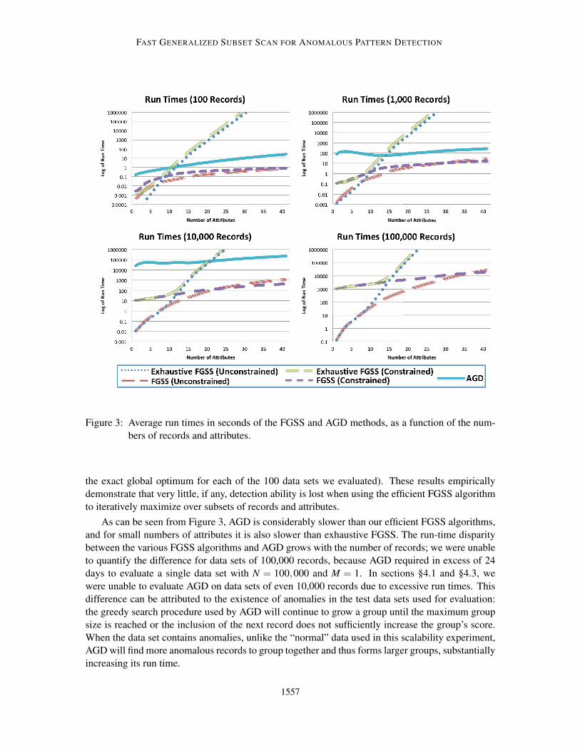
FAST GENERALIZED SUBSET SCAN FOR ANOMALOUS PATTERN DETECTION
Figure 3: Average run times in seconds of the FGSS and AGD methods, as a function of the num-
bers of records and attributes.
the exact global optimum for each of the 100 data sets we evaluated). These results empirically
demonstrate that very little, if any, detection ability is lost when using the efficient FGSS algorithm
to iteratively maximize over subsets of records and attributes.
As can be seen from Figure 3, AGD is considerably slower than our efficient FGSS algorithms,
and for small numbers of attributes it is also slower than exhaustive FGSS. The run-time disparity
between the various FGSS algorithms and AGD grows with the number of records; we were unable
to quantify the difference for data sets of 100,000 records, because AGD required in excess of 24
days to evaluate a single data set with N = 100,000 and M = 1. In sections §4.1 and §4.3, we
were unable to evaluate AGD on data sets of even 10,000 records due to excessive run times. This
difference can be attributed to the existence of anomalies in the test data sets used for evaluation:
the greedy search procedure used by AGD will continue to grow a group until the maximum group
size is reached or the inclusion of the next record does not sufficiently increase the group’s score.
When the data set contains anomalies, unlike the “normal” data used in this scalability experiment,
AGD will find more anomalous records to group together and thus forms larger groups, substantially
increasing its run time.
1557

MCFOWLAND III, SPEAKMAN AND NEILL
4.5 Pattern Characterization
Anomalous pattern detection can be described as a form of knowledge discovery, where the knowl-
edge of interest includes not only the subset of data records affected by an anomalous process,
but also which subset of attributes are anomalous for these records. Accurately describing which
facets of a subset of data are anomalous can be crucial, particularly when discovering a previously
unknown pattern type. In addition to identifying the subset of records affected by an anomalous pro-
cess, our FGSS method also identifies the subset of attributes for which these records are anomalous.
The previously proposed APD method also characterizes anomalous patterns by identifying “rules”
which correspond to a higher than expected number of individually anomalous records. However,
we hypothesize that the identified attributes may not correspond well to the subset of attributes
which are anomalous. To test this hypothesis, we compare the pattern characterization ability of
FGSS and APD using the semi-synthetic PIERS data. Recall that to generate an anomalous group
in the PIERS data, we selected a subset of attributes at random, and regenerated these attribute val-
ues for each affected record. The affected subset of attributes for each record is used as the ground
truth to which we can compare the subset of attributes identified as anomalous by a given method.
We measure each method’s attribute overlap coefficient, defined as
Overlap =|Predicted Attributes ∩ True Attributes|
|Predicted Attributes ∪ True Attributes|,
for each of the PIERS injection scenarios.
However, it is also important to take into consideration the structure of the Bayesian network
used to determine the anomalous patterns. The structure of the network is important in characteriz-
ing the pattern, as it represents the conditional dependencies between attributes. When an attribute
has an anomalous value, either its corresponding likelihood or the likelihoods of its children given
the Bayesian network structure will be low. Therefore, our evaluation framework gives a method
credit for identifying either the affected attribute or at least one of its children. To do so, prior to
computing the overlap coefficient, each method’s set of predicted attributes is redefined according
to the following logic. Given the set of predicted attributes A and the set of true (affected) attributes
B, if there exists an attribute Ai ∈ A with a parent Ap ∈ B, then A = A∪{Ap}, that is, the parent
attribute is counted as correctly predicted. If it is also the case that Ai 6∈ B, then A = A \ {Ai}, that
is, the method is not penalized for identifying the child attribute.
Figure 4 shows a comparison of each method’s overlap coefficient for the PIERS data, averaged
across the different numbers of groups and attributes injected. We also include a simple p-value
characterization method in our comparison: this approach evaluates each record in isolation and
predicts any attribute whose entire p-value range is less than or equal to αmax. We feel that this
is a more appropriate “straw man” than APD to demonstrate the improvements in characterization
ability provided by FGSS. FGSS places all ungrouped records in a group together, and thus we also
use the p-value characterization method to identify a subset of attributes for each ungrouped record.
We allow APD to use all detected patterns in order to identify a subset of attributes for each record,
using the most significant pattern for which that record is a member. We observe that FGSS-BJ
and FGSS-HC consistently demonstrate significantly better performance than the p-value method,
and the p-value method consistently outperforms APD by a large margin. These results support
our hypothesis that the grouping of records that are self-similar and anomalous for some subset of
attributes in our FGSS framework results in substantially improved pattern characterization ability.
1558

FAST GENERALIZED SUBSET SCAN FOR ANOMALOUS PATTERN DETECTION
Figure 4: Pattern characterization accuracy for each method, evaluated on the PIERS data set, and
averaged across different numbers of groups and attributes injected.
5. Conclusions
This paper has presented several contributions to the literature on anomalous pattern detection. We
formalize the pattern detection problem as a search over subsets of data records and attributes, and
present the Fast Generalized Subset Scan (FGSS) algorithm, which efficiently detects anomalous
patterns in general categorical data sets. The FGSS algorithm provides a systematic procedure to
map data set values to an unbiased measure of anomalousness, empirical p-value ranges. The al-
gorithm then uses the distribution of these empirical p-value ranges under the null hypothesis in
order to find subsets of data records and attributes that as a group significantly deviate from their
expectation as measured by a nonparametric scan statistic. We demonstrate that a general class of
nonparametric scan statistics satisfy the linear-time subset scanning property (LTSS). This prop-
erty allows us to search efficiently and exactly over all subsets of data records or attributes while
evaluating only a linear number of subsets. These efficient optimization steps are then incorporated
into an iterative procedure which jointly maximizes over subsets of records and attributes. Addi-
tionally, similarity constraints can be easily incorporated into our FGSS framework, allowing for
the detection of self-similar subsets of records which have anomalous values for some subset of
attributes.
We provide an extensive comparison between FGSS and other recently proposed pattern detec-
tion (AGD, APD) and individual record anomaly detection (BN) methods for general categorical
data on semi-synthetic and real-world data sets. Our results indicate that FGSS consistently out-
performs the other methods. FGSS excels in scenarios when there is a strong self-similarity among
the records generated by an anomalous process, with each individual record only emitting a subtle
anomalous signal. FGSS demonstrates improved scalability as compared to AGD, the method with
the most comparable detection ability. Furthermore, we empirically demonstrate that, even as FGSS
scales to high-dimensional data, it finds the globally optimal subset of records and attributes with
high probability. This optimization task can be performed exactly when the number of attributes
1559

MCFOWLAND III, SPEAKMAN AND NEILL
is small (e.g., twelve attributes or fewer) using the “exhaustive FGSS” approach described above.
When the number of attributes is large, FGSS converges to a conditional maximum (for which the
subset of records is optimal given the subset of attributes and vice-versa), and multiple restarts are
used to approach the joint optimum. Finally, FGSS not only achieves high detection power but
is also able to accurately characterize the subset of attributes for which each identified subset of
records is anomalous.
In future work, we plan to extend FGSS in three main directions. Currently FGSS can only han-
dle categorical attributes, which forces it to discretize continuous attributes when evaluating mixed
data sets. This constraint only exists because our current method for obtaining record-attribute
likelihoods, modeling the conditional probability distribution between attributes with a Bayesian
network and using Optimal Reinsertion (Moore and Wong, 2003) to learn the network structure,
can only handle categorical attributes. By discretizing continuous attributes, we may lose vital
information that would make the task of detecting anomalous patterns easier. Therefore we are cur-
rently investigating extensions of FGSS which better exploit the information contained in continu-
ous attributes. We believe that augmenting a Bayesian network, learned only from the categorical
attributes, with a regression tree for each continuous attribute will increase the power of FGSS to
detect patterns. Second, we are investigating other variants of the nonparametric scan statistic which
take into account the dependence between p-values for a given record and correctly adjust for the
multiplicity of tests. Such statistics might increase detection power as compared to the simpler HC
and BJ statistics used here, but it is not clear whether they can be optimized efficiently over subsets
of the data. Finally, we are also concerned with FGSS being able to better detect novel patterns of
interest. Currently, FGSS only maintains a model M0 describing the distribution of the data when no
anomalous patterns are present, but we plan to extend this approach to maintain models for multiple,
known pattern types. We will detect subsets of records and attributes that are unlikely given each
known pattern model as well as M0, thus enabling FGSS to discover previously unknown pattern
types given the current set of known patterns.
Acknowledgments
The authors would like to thank Sriram Somanchi for fruitful discussions and valuable feedback.
This work was partially supported by the National Science Foundation, grants IIS-0916345, IIS-
0911032, and IIS-0953330. Additionally, Edward McFowland III was supported by an NSF Grad-
uate Research Fellowship (NSF GRFP-0946825) and an AT&T Labs Fellowship.
References
KDD Cup, 1999. URL http://kdd.ics.uci.edu/databases/kddcup99/kddcup99.html.
R. H. Berk and D. H. Jones. Goodness-of-fit test statistics that dominate the Kolmogorov statistics.
Z. Wahrsch. Verw. Gebiete, 47:47–59, 1979.
D. H. Chau, S. Pandit, and C. Faloutsos. Detecting fraudulent personalities in networks of online
auctioneers. In Proceedings of the European Conference on Machine Learning and Principles
and Practice of Knowledge Discovery in Databases, pages 103–114, 2006.
1560

FAST GENERALIZED SUBSET SCAN FOR ANOMALOUS PATTERN DETECTION
K. Das. Detecting patterns of anomalies. Technical Report CMU-ML-09-101, PhD thesis, Carnegie
Mellon University, Department of Machine Learning, 2009.
K. Das and J. Schneider. Detecting anomalous records in categorical datasets. In Proceedings of
the 13th ACM SIGKDD Conference on Knowledge Discovery and Data Mining, pages 220–229,
2007.
K. Das, J. Schneider, and D. B. Neill. Anomaly pattern detection in categorical datasets. In Proceed-
ings of the 14th ACM SIGKDD Conference on Knowledge Discovery and Data Mining, 2008.
A. C. Davison and D. V. Hinkley. Bootstrap Methods and Their Applications. Cambridge University
Press, 1997.
D. Donoho and J. Jin. Higher criticism for detecting sparse heterogeneous mixtures. Annals of
Statistics, 32(3):962–994, 2004.
W. R. Hogan, G. F. Cooper, G. L. Wallstrom, M. M. Wagner, and J.-M. Depinay. The bayesian
aerosol release detector: An algorithm for detecting and characterizing outbreaks caused by an
atmospheric release of bacillus anthracis. Statistics in Medicine, 26:5225–5252, 2007.
M. Kulldorff. A spatial scan statistic. Communications in Statistics: Theory and Methods, 26(6):
1481–1496, 1997.
M. Kulldorff and N. Nagarwalla. Spatial disease clusters: detection and inference. Statistics in
Medicine, 14:799–810, 1995.
A. W. Moore and W.-K. Wong. Optimal reinsertion: A new search operator for accelerated and
more accurate bayesian network structure learning. In Proceedings of the 20th International
Conference on Machine Learning, pages 552–559. AAAI Press, 2003.
D. B. Neill. Expectation-based scan statistics for monitoring spatial time series data. International
Journal of Forecasting, 25:498–517, 2009.
D. B. Neill. Fast Bayesian scan statistics for multivariate event detection and visualization. Statistics
in Medicine, 30(5):455–469, 2011.
D. B. Neill. Fast subset scan for spatial pattern detection. Journal of the Royal Statistical Society
(Series B: Statistical Methodology), 74(2):337–360, 2012.
D. B. Neill and G. F. Cooper. A multivariate Bayesian scan statistic for early event detection and
characterization. Machine Learning, 79:261–282, 2010.
D. B. Neill and J. Lingwall. A nonparametric scan statistic for multivariate disease surveillance.
Advances in Disease Surveillance, 4:106, 2007.
D. B. Neill, A. W. Moore, M. R. Sabhnani, and K. Daniel. Detection of emerging space-time
clusters. In Proceedings of the 11th ACM SIGKDD Conference on Knowledge Discovery and
Data Mining, 2005.
D. B. Neill, G. F. Cooper, K. Das, X. Jiang, and J. Schneider. Bayesian network scan statistics
for multivariate pattern detection. In J. Glaz, V. Pozdnyakov, and S. Wallenstein, editors, Scan
Statistics: Methods and Applications, 2008.
1561