Fast Distance Field Computation Using Graphics Hardware

Avneesh Sud and Dinesh ManochaDepartment of Computer Science, Univeristy of North Carolina

Chapel Hill, NC, USA{sud,dm}@cs.unc.edu

http://gamma.cs.unc.edu/DiFi

UNC Computer Science Technical Report TR03-026

Abstract

We present an algorithm for fast computation of dis-cretized 3D distance fields using graphics hardware. Givena set of primitives and a distance metric, our algorithmcomputes the distance field for each slice of a uniform spa-tial grid by rasterizing the distance functions of the prim-itives. We compute bounds on the spatial extent of theVoronoi region of each primitive. These bounds are usedto cull and clamp the distance functions rendered for eachslice. Our algorithm is applicable to all geometric modelsand does not make any assumptions about connectivity ora manifold representation. We have used our algorithm tocompute distance fields of large models composed of tensof thousands of primitives on high resolution grids. More-over, we demonstrate its application to medial axis evalu-ation and proximity computations. As compared to earlierapproaches, we are able to achieve an order of magnitudeimprovement in the running time.

Keywords: Distance fields, Voronoi regions, graphics hard-ware, proximity computations

1 IntroductionGiven a set of objects, a distance field in 3D is defined ateach point by the smallest distance from the point to theobjects. Each object may be represented as data on a voxelgrid or as an explicit surface representation. Moreover, thedistances between the point and an object can be specifiedusing different metrics, including Euclidean or max-normdistance. If the primitives are closed or orientable, a signcan be assigned to the distance field.

Distance fields are frequently used in computer graphics,geometric modeling, robotics and scientific visualization.Their applications include shape representation [10, 29, 30],model simplification [14], remeshing [20, 30], morphing[5], CSG operations [1, 2], sculpting [25], swept volume

computation [19], path planning and navigation [15, 18],collision and proximity computations [16, 17], etc. Theseapplications use a signed or unsigned distance field along adiscrete grid.

Different algorithms have been proposed to compute thedistance fields in 2D or 3D for geometric and volumetricmodels. The computation of a distance field along a uni-form grid can be accelerated by using graphics rasterizationhardware [15, 8, 28]. These algorithms compute 2D slicesof the 3D distance field by rendering the three dimensionaldistance function for each primitive. However, renderingthe distance meshes of all the primitives for each slice maybecome expensive in terms of transformation and rasteriza-tion cost. As a result, current algorithms for 3D distancefield computation may be slow and not work well for de-formable models or dynamic environments.Main Contributions: We present a fast algorithm (DiFi)to compute a distance field of complex objects along a 3Dgrid. We use a combination of novel culling and clampingalgorithms that render relatively few distance meshes foreach slice. We also exploit spatial coherence between adja-cent slices in 3D and perform incremental computations tospeed up the overall algorithm.

Our novel site culling algorithm uses properties of theVoronoi diagram to cull away primitives that do not con-tribute to the distance field of a given slice. We use a two-pass approach and perform culling using occlusion queries.Furthermore, we present a conservative sampling strategythat accounts for sampling errors in the occlusion queries.Our clamping algorithm reduces the rasterization cost ofeach distance function by rendering it on a portion of eachslice.

We have implemented DiFi on a 2.8GHz PC with anNVIDIA GeForce FX 5900 Ultra graphics processor andused it to compute distance fields of complex objects con-sisting of tens to hundreds of thousands of triangles. Therunning time ranges from a second for small models to tens

Figure 1. 3D Distance Field of Hugo Model(17k poly-gons): Distance to the surface is color coded, increasingfrom red to green to blue. Time taken to compute the dis-tance field on 73×45×128 grid using our algorithm is 4.2seconds.

of seconds for large models. We have used DiFi to computethe simplified medial axis of complex polyhedral modelsand perform proximity computations in a dynamic environ-ment for path planning. As compared to prior distance fieldcomputation algorithms, our approach offers the followingadvantages:

• Generality: No assumption is made with regards tothe input models. The objects may be non-orientableor non-manifold surfaces, or may be represented usingvoxel data.

• Efficiency: We show that our approach is significantlyfaster than previous approaches. The culling tech-niques provide us with a 3 − 20 times speedup in dis-tance field computation over previous approaches thatcan handle generic models. The speedups are higherfor complex models with a high number of primitives.

• Dynamic Models: Our algorithm involves no prepro-cessing and can compute distance fields of dynamicobjects with a few thousand polygons at almost inter-active rates.

Organization: The rest of the paper is organized in the fol-lowing manner. We give a brief survey of distance fieldcomputation algorithms in Section 2 and an overview ofour approach in Section 3. Section 4 describes our cullingalgorithm and Section 5 presents the clamping algorithm.In Section 6, we highlight two applications of our distancefield computation algorithm. We describe its performancein Section 7 and analyze it in Section 8.

2 Related WorkThe problem of computing a distance field can be broadlyclassified by the type of input object representation. Theobject can be specified either as a data on a voxel grid, such

as a binary image or as an explicit surface representation,such as a triangulated model.

2.1 Distance Fields of Geometric ModelsMany algorithms are known to compute the distance fieldsof geometric models represented using polygonal or higherorder surfaces. These algorithms use either a uniform gridor an adaptive grid. A key issue in generating discrete dis-tance samples is the underlying sampling rate used for adap-tive subdivision. Many adaptive refinement strategies usetrilinear interpolation or curvature information to generatean octree spatial decomposition [27, 10, 25, 31].

Distance field computation can be accelerated usinggraphics hardware. The graphics hardware based algo-rithms compute a 2D slice of the distance field at a time.Hoff et al. [15] render a polygonal approximation of thedistance function on the depth-buffer hardware and com-pute the generalized Voronoi Diagrams in two and three di-mensions. This approach works on any geometric modelthat can be polygonized and is applicable to any distancefunction that can be rasterized. An efficient extension ofthe 2-D algorithm for point sites is proposed in [8]. Ituses precomputed depth textures, and a quadtree to esti-mate Voronoi region bounds. However, the extension ofthis approach to higher dimensions or higher order primi-tives is not presented. A class of exact distance transformalgorithms is based on computing partial Voronoi diagrams[21]. A scan-conversion method to compute the 3-D Eu-clidean distance field in a narrow band around manifold tri-angle meshes is the Characteristics/Scan-Conversion (CSC)algorithm [22]. The CSC algorithm uses the connectivityof the mesh to compute polyhedral bounding volumes forthe Voronoi cells. The distance function for each site isevaluated only for the voxels lying inside this polyhedralbounding volume. An efficient GPU based implementationof the CSC algorithm is presented in [28]. The number ofpolygons sent to the graphics pipeline is reduced and thenon-linear distance functions are evaluated using fragmentprograms.

2.2 Volumetric ModelsGiven voxel data, many exact and approximate algorithmsfor distance field computation have been proposed [24, 2,12]. A good overview of these algorithms has been given in[6]. The approximate methods compute the distance field ina local neighborhood of each voxel. Danielsson [7] uses ascanning approach in 2D based on the assumption that thenearest object pixels are similar. The Fast Marching Method(FMM)[26] propagates a contour to compute the distancetransformation from the neighbors. This provides an ap-proximate finite difference solution to the Eikonal Equation|∇u| = 1/f . A linear time algorithm for computing ex-act Euclidean distance transform of a 2-D binary image ispresented in [3]. This is extended to k-D images and other

distance metrics [23].

3 Overview and NotationIn this section we introduce the notation used in the paperand give an overview of our approach.3.1 Distance FieldsA geometric primitive or an object in 3D is called a site.Given a site pi, the scalar distance function dist(q, pi) de-notes the distance from the point q ∈ R

3 to the closestpoint on pi. The minimum distance of q to a set of sitesP = {p1, p2, . . . , pm} is represented as dist(q,P) =minpi∈P(dist(q, pi)). The distance field DM (P), for a do-main M ⊂ R

3, is the scalar field given by the minimumdistance function dist(q,P) for all points q ∈ M . For easeof notation, let DM = DM (P). Given a subset, X ⊂ P ,dist(q,X ) ≥ dist(q,P)∀q ∈ M .

Distance fields are closely related to Voronoi regions.The Voronoi region for pi is defined as:

V (pi) = {q | dist(q, pi) ≤ dist(q, pj)∀pj ∈ P,q ∈ M}Our goal is to compute the distance field within a boundeddomain M represented as an axis-aligned uniform 3D grid.Let the size of each voxel in the 3D grid be δx × δy × δz .In a bounded domain, Voronoi regions are bounded. Let theminimum and maximum bounds of the Voronoi region ofa site pi along Z be V (pi).zmin and V (pi).zmax, respec-tively.3.2 Computation using Graphics HardwareA brute-force algorithm to compute DM would evaluatedist(q, pi) for all sites pi ∈ P and store the minimum ateach grid point q ∈ M . If there are m sites, and the gridhas n cells, the time complexity of this algorithm is O(mn).This brute force algorithm can be easily parallelized usingdepth-buffered graphics rasterization hardware [15]. Theprimitive sites in P consist of points, edges and triangles.The set of voxels with a constant z-value represents a uni-form 2D grid and is called a slice. A slice sk is defined assk = {(x, y, z)|(x, y, z) ∈ M, z = zk}. In the rest of thepaper, we represent the distance field Dsk

(P) for a slice sk

as Dk(P). A sweep is performed along the Z axis and thedistance field Dk is computed for each slice. The complex-ity of this algorithm is linear in m for each slice and therunning time can be slow when m is large.3.3 Our ApproachWe speed up the 3D distance field computation by reduc-ing the number of distance functions that are rasterized foreach slice. We exploit the following properties of Voronoiregions and distance fields to accelerate the computation:

1. Connectivity: We consider distance metrics that aresymmetric, positive definite and satisfy the triangle in-equality. Thus, Voronoi regions defined by that dis-tance metric are connected. This is true for all Lp

norms, including Euclidean distance and max-norm[4]. Note that for higher order sites, like line segmentsand polygons, each Voronoi region may consist of non-linear boundaries and may not be convex. But eachVoronoi region is connected.

2. Spatial Coherence: The distance fields of adjacentslices, sk and sk+1, can have high spatial coherence.The distance values associated with two points in ad-jacent voxels on a 3D grid will be very close to eachother. We use this coherence to compute bounds onthe maximum change in the distance field between ad-jacent slices.

3. Monotonicity: Given a slice, the distance functionof a site is a monotonic function. It has a minimumvalue in the interior of the slice and is maximum onthe boundary of the slice.

Our goal is to cull away sites that do not contribute tothe final distance field for a particular slice. Furthermore,the distance field for each site should be computed in theregion of the slice where it contributes to the final distancefield (see Figure 2). Our algorithm utilizes the above men-tioned properties and computes conservative bounds on theVoronoi regions. We use these bounds in two steps: to cullthe set of sites for each slice (described in Section 4) andclamp the region of computation for each site in the non-culled set (described in Section 5).3.4 Site ClassificationWe introduce a classification of the sites used by our algo-rithm to cull away sites that do not contribute to the distancefield for a slice. Let us assume that the sweep direction isalong the +Z direction. For a slice sk at z = zk, we par-tition the set of sites P into three subsets depending on theVoronoi region bounds of each site along the Z axis (shownin Figure 2):

Intersecting, I+

k = {pi | V (pi).zmin ≤ zk ≤V (pi).zmax}. Only the distance functions of thesesites contributes to the final distance field of slice sk.

Approaching, A+

k = {pi | V (pi).zmin > zk}. TheVoronoi region of an approaching site does not inter-sect with current slice, but could potentially intersectwith a slice sl, where zl > zk.

Receding, R+

k = {pi | V (pi).zmax < zk}. Due to theconnectivity property of Voronoi regions, a recedingsite can never become intersecting, hence it can be dis-carded for any slice sl, where zl > zk.

For efficient computation, the algorithm presented inSection 4 performs two passes along +Z and −Z direc-tions and considers only the sites swept up-to the current

Figure 2. Site Classification: Shaded areas repre-sent the connected Voronoi regions for a subset of sites{p1, . . . , p5}. Sweep direction is along +Z. For slicesk, the site sets are: Intersecting I+

k = {p2, p3, p4},Approaching A+

k = {p5}, Receding R+

k = {p1} andSwept S+

k = {p1, p2, p3}, Unswept U+

k = {p4, p5}. Dis-tance functions have to be drawn for set I+

k only. For sitep3, the distance function has be drawn only in the regionQ3,k = V (p3) ∩ sk. For the next slice sk+1, p4 is movedto S+

k+1, p5 is moved to I+

k+1and p3 is moved to R+

k+1.

slice. We also partition P based on the spatial bounds ofeach site along Z axis. Let pi.zmax denote the maximum Zvalue of a site pi. Then the set P is partitioned as (shown inFigure 2):

Swept, S+

k = {pi | pi.zmax ≤ zk}

Unswept, U+

k = {pi | pi.zmax > zk}

The intersecting set I+

k can be further partitioned into anintersecting swept set IS+

k = (I+

k ∩S+

k ) and an intersectingunswept set IU+

k = (I+

k ∩ U+

k ).

I+

k = IS+

k ∪ IU+

k (1)

The set of sites, P , is also partitioned into subsets along the−Z sweep direction. The intersecting, swept and unsweptsubsets are represented as I−

k , S−k , U−

k , and are defined as

I−k = {pi | V (pi).zmin ≤ zk ≤ V (pi).zmax}

S−k = {pi | pi.zmax > zk}

U−k = {pi | pi.zmax ≤ zk}

Consequently,

U+

k = S−k , I+

k = I−k = Ik

and Eq. (1) reduces to

Ik = IS+

k ∪ IS−k (2)

The key idea for speedup is that for a large number of sitesm and any given slice sk, the size of Ik is typically muchsmaller than m. By computing a conservative estimate of Ik

one can cull away a large number of sites and considerablyspeed up the distance field computation.

4 Site CullingIn this section, we present our culling algorithm that reducesthe number of distance functions that are rasterized for eachslice. Our goal is to compute the distance field Dk for eachslice sk. Since only the set Ik contributes to Dk, we haveDk = Dk(Ik). Using Eq. (2), Dk can be expressed as:

Dk(Ik) = Dk(IS+

k ∪IS−k ) = min

(Dk(IS+

k ), Dk(IS−k )

)

Therefore, the problem is reduced to computing two dis-tance fields Dk(IS+

k ) and Dk(IS−k ) for each slice sk. We

present an algorithm to compute Dk(IS+

k ) for sk with asweep direction along +Z. The same algorithm is used tocompute Dk(IS−

k ) by using a sweep direction along −Z.In the rest of the paper, we will present our algorithm for+Z sweep direction and drop the + sign to simplify thenotation.

We utilize the spatial coherence between successiveslices and compute the intersecting swept set ISk+1 by per-forming incremental computations on ISk (see Figure 2).We use the following formulation:

(ISk+1) =(ISk ∪ (Sk+1 \ Sk)

)\ (Rk+1 \ Rk) (3)

where \ represents the set-difference operation. The ex-act computation of ISk and ISk+1 is equivalent to exactVoronoi computation. Instead, we conservatively compute aset of potentially intersecting swept sites ISk using Equa-tion (3), where ISk ⊇ ISk.

Given the sets ISk and Rk, the algorithm for comput-ing Dk+1, ISk+1 and Rk+1

proceeds as follows:

1. Initialize ISk+1 = ISk, Dk+1 = ∞.

2. Update ISk+1 = ISk+1 ∪ (Sk+1\ Sk). Add the

additional sites swept by slice sk+1 to ISk+1 .

3. Compute Dk+1. For each site pi ∈ ISk+1, com-pute Dk+1(pi) in order of increasing i. Each Dk(pi) istested for visibility with respect to Dk+1(Xi−1), whichis the distance field of set Xi−1 = {p1, p2, . . . , ˆpi−1}.If Dk+1(pi) is not visible along the direction orthogo-nal to sk+1, then it does not contribute to Dk+1.

4. Compute (Rk+1\ Rk). All sites pi for which

Dk+1(pi) is not visible can be moved from ISk+1

to Rk+1.

5. Update ISk+1 = ISk+1 \ (Rk+1\ Rk)

Initially we set k = 0,Rk = ∅, ISk = {pi|pi.zmax = 0}.We proceed along the Z-axis and compute the distance fieldfor each slice as described above. Each site pi is bucketedinto a list according to pi.zmax. This allows the addition

Figure 3. Sampling Error: (a) The Voronoi region V (p2)of a swept site p2 does not lie on any cell (represented bycrosses) on slice sk, but lies on a cell for slice sk+1. (b) TheXY intersection of the Voronoi regions with slice sk. Theclosest cell q to V (p2) is at a distance ε.

of swept sites in Step (2) to be performed in constant time.The distance fields are rasterized approximately in order ofincreasing distance to the current slice. This results in bet-ter culling of the receding sites in Steps (3) and (4) of thealgorithm. The complexity of this algorithm for slice sk+1

is a linear function of the size | ISk+1 |.The visibility computations are performed using occlu-

sion queries (e.g. GL NV occlusion query) available oncurrent graphics systems. As the distance meshes are scanconverted, these queries check for updates to the depthbuffer and return the number of pixels that are visible.4.1 Conservative SamplingThe occlusion queries sample the visibility at fixed loca-tions in each pixel and can result in sampling errors. Inparticular, the algorithm presented above classifies a sweptsite pi as receding if its Voronoi region V (pi) does not coverany grid cells, i.e. the occlusion query returns zero visiblepixels for the distance field Dk(pi) in Step (3). This mayintroduce errors when V (pi) intersects slice sk but its inter-section with sk is not sampled by the rasterization hardware.An incorrect classification of pi as receding can introduceerrors in Dl for a subsequent slice sl, l > k. One such caseis shown in Figure 3(a), for i = 2.

We modify the algorithm for distance field computationto account for these sampling errors. The approach is basedon a lemma that states the condition for a Voronoi region tobe sampled.

Lemma 1. Let V (pi) be a voronoi region for a slice sk thatis undersampled, and the closest cell q is at a distance εfrom V (pi). If we reduce dist(q, pi) by ε without changingdist(q,P − pi), we ensure that q ∈ V (pi).

Proof. Let q belong to the voronoi region V (pj) of site pj ,and the point in V (pi) closest to q be r (see Figure 3), withi = 2, j = 4, dist(q, r) = ε. We shall first prove the re-sult for the case when V (pi) shares a boundary with V (pj).

Figure 4. Conservative Sampling: (a) Distance fieldDk(p2) of site p2 is occluded at all pixels on sk. (b) Trans-lating Dk(p2) by δxy ensures it is visible at at least onepixel.

Then using the fact r ∈ V (pi) and r ∈ V (pj), and thetriangle inequality, we have

dist(r, pj) = dist(r, pi)

dist(q, pi) ≤ dist(q, r) + dist(r, pi)

dist(r, pj) ≤ dist(r,q) + dist(q, pj)

⇒ dist(q, pi) − ε ≤ dist(r, pj) < dist(q, pj)

Thus, by reducing dist(q, pi) by ε and keeping dist(q, pj)the same, q will lie in Voronoi region V (pi). This directlyextends to the case when V (pi) and V (pj) do not sharea boundary, by using a sequence of triangle inequalitiesacross Voronoi boundaries between V (pi) and V (pj).

We apply the result of Lemma 1 in the following manner. Inpractice, we do not know the point q or ε but use the fact that

ε is bounded by pixel size, ε ≤ δxy =

√δ2

x+δ2y

2. Therefore,

we move pi closer to all the points in slice sk, by subtractingδxy from each value of the distance field Dk(pi). This isequivalent to translating Dk(pi) along −Z by δxy and isshown in Figure 4.

Given a slice sk+1, we redraw the translated distancefield of each site pi marked as receding in Step (4) of thealgorithm given above (i.e. pi ∈ Rk+1

\ Rk). The redrawndistance field is tested for visibility with respect to Dk+1.This redrawing is performed to ensure conservative sam-pling for site-culling. During this step, updates to the finaldistance field in the depth buffer are disabled. Moreover,the translated field is clamped to 0 for negative values. Forline and triangle sites, the size of the Voronoi region is alsolimited by the spatial size of the line segment or the triangle.To ensure that the Voronoi region covers at least one of thefour neighboring cells, we increase the size of these sites byδxy in addition to translating the distance field.

5 Distance Function ClampingIn Section 4, we presented an algorithm to cull away thesites that do not contribute to the distance field Dk of slice

sk. In this section, we present a clamping algorithm to re-duce the rasterization cost of the distance function of eachpotentially intersecting swept site. Given a slice sk and eachsite pi ∈ ISk, we compute the distance function dist(q, pi)only for the set of points on sk that lie in the Voronoi re-gion of pi. In other words, our goal is to evaluate the dis-tance function for the set Qi,k = {q|q ∈ V (pi) ∩ sk}. Wefirst present an approach to compute a conservative estimateQi,k of Qi,k for any arbitrary set of sites. We further im-prove the performance of the clamping algorithm for mani-fold surfaces by using the CSC-algorithm [22].5.1 Conservative ClampingThe connectivity of the Voronoi regions implies that Qi,k

is a connected set. We exploit the monotonicity propertyand compute a superset Qi,k. Initially, we assume that weare given the maximum value max(Dk(pi)) of the distancefield Dk(pi) of site pi on slice sk. We compute a set ofextreme points on sk where the value of the distance fieldDk(pi) is equal to the maximum value. By the monotonic-ity property of distance functions, the set of points whosedistance function is less than or equal to max(Dk(pi)) be-long to Qi,k. An example is shown in Figure 5.

Figure 5. Clamping distance field computation to Voronoiregion bounds on a slice. Q2,k = V (pi)∪sk. Q2,k ⊇ Q2,k

and is computed from max(Dk(p2)).

The problem of distance function clamping reduces tocomputing max(Dk(pi)) for each site pi in ISk for a slicesk. We use the following lemma to compute an upper boundon max(Dk(pi)).

Lemma 2. Let max(Dk(Sk)) denote the maximum valueof the distance fields Dk(Sk) of set Sk on a slice sk andmax(Dk+1(Sk+1

)) be defined similarly. Let the distancebetween sk+1 and sk be |zk+1 − zk| = δz . Then

max(Dk+1(Sk+1)) ≤ max(Dk(Sk)) + δz (4)

Proof. Given two points qk(x, y, zk) ∈ sk andqk+1(x, y, zk+1) ∈ sk+1 that lie in the Voronoi regions ofsome two sites. Then

|dist(qk+1,P) − dist(qk,P)| ≤ δz. (5)

Figure 6. Change in distance field for signed distancecomputation

This follows directly from the triangle inequality, and thedefinition of the distance function dist(q,P). Moreover,max(Dk(X )) = maxq∈sk

(dist(q,X )). This implies that

max(Dk+1(X )) ≤ max(Dk(X )) + δz (6)

Moreover, for a slice sk and any two sets of sites X1 and X2,X1 ⊆ X2 ⇒ Dk(X2) ≤ Dk(X1). We know Sk ⊆ Sk+1

.This combined with Eq. (6), where X = Sk+1

, leads to theresult in Eq. (4).

Given the maximum value max(Dk(Sk)) of the distancefield for slice sk, we use Eq. (4) to compute the maxi-mum value max(Dk+1(Sk+1

)) of the distance field for slicesk+1. This also gives a conservative bound on maximumvalue of the distance function for each site pi on slice sk+1,max(Dk+1(Sk+1

)) ≥ max(Dk+1(pi)) ∀ pi ∈ Sk+1. We

use it to compute a conservative bound on the set of pointsQi,k+1 on slice sk+1 and use this bound for clamping.

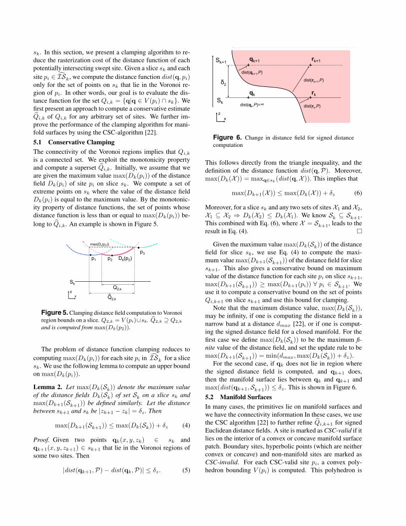
Note that the maximum distance value, max(Dk(Sk)),may be infinity, if one is computing the distance field in anarrow band at a distance dmax [22], or if one is comput-ing the signed distance field for a closed manifold. For thefirst case we define max(Dk(Sk)) to be the maximum fi-nite value of the distance field, and set the update rule to bemax(Dk+1(Sk+1

)) = min(dmax,max(Dk(Sk)) + δz).For the second case, if qk does not lie in region where

the signed distance field is computed, and qk+1 does,then the manifold surface lies between qk and qk+1 andmax(dist(qk+1,Sk+1

)) ≤ δz . This is shown in Figure 6.5.2 Manifold SurfacesIn many cases, the primitives lie on manifold surfaces andwe have the connectivity information In these cases, we usethe CSC algorithm [22] to further refine Qi,k+1 for signedEuclidean distance fields. A site is marked as CSC-valid if itlies on the interior of a convex or concave manifold surfacepatch. Boundary sites, hyperbolic points (which are neitherconvex or concave) and non-manifold sites are marked asCSC-invalid. For each CSC-valid site pi, a convex poly-hedron bounding V (pi) is computed. This polyhedron is

Figure 7. Medial Axis Transform: Left: Triceratops model (5.6k polygons, Grid Size=128× 56× 42, Computation Time=0.79s)The medial surface is color coded by the distance from the boundary. Right: Brake rotor model (4.7k polygons, Grid Size=4 ×128 × 128, Computation Time=0.61s ). The medial seam curves are shown in red.

intersected with sk+1 to compute a convex polygon Gi,k+1.In this case, Gi,k+1 ∩ Qi,k+1 results in a tighter approxima-tion of Qi,k+1.

5.3 Complete AlgorithmGiven ISk , Rk and Dk, the algorithm for computingDk+1 as presented in Section 4 is refined to perform clamp-ing as follows:

1. Compute max(Dk) by using multiple occlusionqueries as described in [13]. Compute max(Dk+1) =min(dmax,max(Dk) + δ).

2. Initialize ISk+1 = ISk, Dk+1 = ∞.

3. Update ISk+1 = ISk+1 ∪ (Sk+1\ Sk).

41. Compute Qi,k+1. For each site pi ∈ ISk+1, computeQi,k+1 from max(Dk+1)

42. Refine Qi,k+1. For each CSC-valid site pi ∈ ISk+1,compute the convex polygon Gi,k+1. Refine Qi,k+1 =

Qi,k+1 ∩ Gi,k+1.

43. Compute Dk+1. For each site pi ∈ ISk+1, computeD

Qi,k+1(pi) and test for visibility as before.

44. Perform Conservative Sampling Disable distancefield updates. For each site pi ∈ ISk+1 which ismarked as occluded, expand the site and computeD

Qi,k+1(pi)− δxy . Test for visibility against the com-

puted distance field Dk+1 as before. Enable distancefield updates.

5. Compute (Rk+1\Rk) from the results of the visibility

tests of Step 3.4.

6. Update ISk+1 = ISk+1 \ (Rk+1\ Rk).

Given a 3D grid with N + 1 slices and a Z range[zmin, zmax], we make 2 passes. In the first pass, we

increment k from 0 to N . Initially, R+

0 = ∅, IS+

0 ={pi|pi.zmax = zmin}. In the second pass, k is decre-

mented from N down to 0. Initially, R−N = ∅, IS−

N ={pi|pi.zmax = zmax}. The final distance field for eachslice is the lower envelope of both.

6 ApplicationsWe have applied our distance field algorithm to computethe medial axis transform of polyhedral models and pathplanning. These applications require global distance fieldcomputation along a 3D grid.

Simplified Medial Axis Computation: We computea simplification of the Blum medial axis, called the θ-simplified medial axis (θ-SMA) [9]. The θ-SMA provides agood approximation of the stable subset of the medial axis.The algorithm for computing the θ-SMA of an object X isbased on computing the vector field called the neighbor di-rection field of the object X and denoted by N(X). N(X)is the negated gradient of the distance field defined by theboundary of X . Given N(X), a separation criterion is de-fined using the separation angle θ. The criterion is used tocheck whether a line segment connecting the centers of ad-jacent voxels of a grid crosses a sheet of the medial axis.When a pair of points passes the separation criterion, weadd the facet between them to the approximation of θ-SMAand compute a polygonal approximation of the medial axis.In some cases a discrete voxel representation of the θ-SMAis desirable. A voxel is added to the medial axis if it lies onone side of a facet on the medial axis, which is determinedas above. This selection operation can be efficiently per-formed on modern programmable graphics hardware usingfragment programs. The gradient field is stored on graphicscard texture memory. This avoids the costly readbacks ofthe entire distance field to the CPU.

Interactive Path Planning in Dynamic Environments:We have used our distance field computation algorithmwithin a constraint-based path planner [11]. The path plan-ning problem is reduced to simulating a constrained dy-namic system, and computes an approximation of the gener-alized Voronoi diagrams (GVD) of the robot and obstaclesin the environment. Each robot is subject to virtual forcesintroduced by geometric and mechanical constraints, suchas making the robot follow an estimated path computed us-ing the GVD and linking the rigid objects together to rep-resent an articulated robot. The distance field is used tocompute an approximate GVD and a Voronoi graph. Thedistance field is also used to perform proximity tests be-tween the robot and the obstacles and maintain a minimumclearance. Given a pair of objects, R1 and R2, the distancefield of R2 is drawn in a potentially overlapping region. Thesurface of R1 is sampled at points inside the overlapping re-gion, and a force is generated at each sample point qi. Theforce is in the direction of the gradient of the distance fieldand proportional to the distance between qi and the surfaceof R2. As the obstacles in the environment undergo mo-tion, our algorithm recomputes the distance field and usesit for path computation. We have used this path planner forvirtual prototyping applications.

7 Implementation and Results

In this section we describe the implementation of our dis-tance field computation algorithm and highlight its perfor-mance on complex polygonal models.

We have implemented our algorithm in Microsoft VisualC++ and use OpenGL as the graphics API. The distancefunction for each primitive is approximated as a polygo-nal mesh based on techniques presented in [15]. The vis-ibility test is performed using the OpenGL occlusion queryextension GL NV occlusion query. We exploit the paral-lelism of this query by batching together occlusion queriesfor an entire set of potentially intersecting sites. The CSCalgorithm [22] is used for clamping the region of distancefield computation for CSC-valid sites. We have integratedthe CSC algorithm with the distance field computation al-gorithm presented in [15]. We clamp the approximate dis-tance mesh of each CSC-valid site with the bounding con-vex polyhedra. The bounding convex polyhedra are com-puted at run time. Our implementation involves no precom-putation and is directly applicable to deformable models.

We generate the gradient vector field along with the dis-tance field to compute the θ-SMA. The gradient vector isencoded in the color values of each vertex of the distancemesh. The voxel representation of the θ-SMA is com-puted directly on the graphics processor using OpenGL’sARB fragment program extension. The medial axis is ren-dered directly from the GPU as a volume grid.

7.1 PerformanceWe have applied our algorithm to 3D polygonal models.These include scanned models and CAD models. Some ofthem are non-manifold.Distance Field Computation: All the timings reportedin this paper were generated on a Pentium4 2.8GHz PCwith 2GB RAM and an NVIDIA GeForce FX 5900 Ul-tra graphics card, running Windows XP. We have com-pared the performance of our distance field computationalgorithm (DiFi) with the algorithm presented by Hoffet al. [15](called HAVOC), a software implementation ofCSC algorithm [22], and an implementation that combinesHAVOC with CSC. The timings are presented in Table 1.In our benchmarks, DiFi obtains more than two orders ofmagnitude over a software implementation of the CSC al-gorithm and more than one order of magnitude performanceimprovement over an implementation combining HAVOCand CSC for manifold objects. For non-manifold models,we obtain 4 − 20 times speedup over HAVOC.Medial Axis Computation: We have applied the distancefield to compute the simplified medial axis of polyhedralmodels. The simplified medial axis for two models is shownin Figure 7. Our algorithm takes less than a second tocompute the medial axis of polyhedral models consistingof thousands of polygons.Path Planning: We have applied the path planning algo-rithm to an assembly environment (shown in Figure 9). Theenvironment consists of an articulated robot arm with 6 de-grees of freedom placed in the middle of a complicated pip-ing structure. The robot arm reaches for a part moving on aconveyor belt and avoids collision with obstacles. Variouslinks on the robot arm come in close proximity with the pip-ing structures. We are able to dynamically compute the pathat interactive rates using our fast distance field computationalgorithm.

8 Analysis and LimitationIn this section we analyze the performance of our algorithm.We highlight its computational complexity and the errorsin distance computation. We also compare its performancewith earlier algorithms.

We approximate each non-linear distance function witha polygonal distance mesh. This introduces a tessellationerror [15]. The tessellation error is bounded by a user de-

fined ε > 0. We set ε =

√δ2

x+δ2y+δ2

z

2so that the error in

the distance field is no more than half the diagonal lengthof a grid cell. As a result, the main source of discretizationerror is grid resolution. Current graphics processors support24-bit depth buffers, so the error in depth computation andcomparisons is relatively small.

Given a model with m sites and a 3D grid of sizen = N × N × N , the cost of computing the distancefield is proportional to the number of processed cells over

Model Polys Resolution CSC HAVOC HAVOC+CSC DiFiRotor 4736 4x128x128 59.22 6.33 3.98 0.61Rotor 4736 8x254x254 424.89 18.73 12.12 1.16Triceratops5660 128x56x42 127.81 2.11 1.10 0.79Triceratops5660 254x111x84 990.48 6.33 3.65 1.92Hugo 17000 73x45x128 X 30.55 19.24 4.22Hugo 17000 145x90x254 X 108.84 75.85 8.63Head 21764 78x105x128 201.12 37.89 16.76 4.98Shell 22598 254x252x252 X 162.97 95.31 7.79Cassini 93234 186x254x188 X 356.03 298.55 29.86Dragon 108926 57x90x128 X 171.13 95.69 24.76

Table 1. Distance Field Computation: Times (in seconds) to compute the global dis-tance fields using approaches by Mauch [22] (CSC), Hoff et al. [15](HAVOC), an im-plementation combining CSC with HAVOC on graphics hardware (HAVOC+CSC), andour algorithm (DiFi). For the entries marked X, CSC algorithm fails as the model con-tains CSC-invalid sites.

Figure 8. Cassini Model: Avolume rendering of the dis-tance field of the Cassini with93K polygons. The distance tothe surface is color coded, in-creasing from red to green toblue.

which the distance function is evaluated. The optimal costfor computing the 3D distance field is O(N 3) = O(n).For a slice sk, the optimal number of processed cells is∑|Ik|

i=1|Qi,k| = N2. The actual number of processed cells

is∑|Ik|

i=1|Qi,k|. We define the following average number of

cells covered by one site:

optimal = 〈|Qi,k|〉 =∑|I

k|

i=1|Qi,k|

|Ik| , actual = 〈|Qi,k|〉 =

∑|Ik|

i=1|Qi,k|

|Ik|

The per-slice efficiency of our algorithm can be measuredby two ratios: the clamping efficiency, e1k =

〈|Qi,k|〉

〈|Qi,k|〉and

culling efficiency, e2k =|Ik|

|Ik|. The average efficiency per

slice can be defined as 〈e〉 = 1

N

∑Nk=1

e1k × e2k. The totalcost of the algorithm is O(n/〈e〉), and is bounded betweenO(n) and O(mn). For CSC-invalid sites, the clamping ef-ficiency e1k approaches 1 as the sites are uniformly dis-tributed on the 3D grid. For CSC-valid sites, the complex-ity is similar to that of the CSC algorithm, i.e. O(m + rn).However, our algorithm obtains tighter bounds on the pa-rameter r, r = 1/〈e〉. In practice, e1k ≈ 1, thus r = 1

〈e2k〉.

We sample and render some of the distance functionstwice in order to overcome the sampling errors introducedby occlusion queries. Moreover, to detect under-samplingerrors, the distance field is offset by a larger value of cellsize δxy , leading to a more conservative estimate of thepotentially intersecting set. This extra computation is per-formed only when a site is marked as receding due to under-sampling, and becomes smaller at higher grid resolutions.

8.1 Comparison

We now provide a comparison of our algorithm, DiFi, withtwo previous algorithms for computing 3D distance fields

using graphics hardware: HAVOC, and the algorithm bySigg et al. [28].HAVOC: DiFi is restricted in the distance functions han-dled compared to HAVOC, since it assumes that the Voronoiregions are connected. It can however handle a wide rangeof distance functions, including all the Lp metrics, whilegiving more than one order of magnitude speedup. LikeHAVOC, it is applicable to generic models without connec-tivity information, and has the same error bounds.Sigg et al.: The algorithm by Sigg et al. [28] is applica-ble only to manifold surfaces and has the same asymptoticcomplexity as the CSC algorithm [22], i.e. O(m+rn). It isparticularly efficient for computing the distance field in nar-row bands around manifold surfaces. For small band sizes,the parameter r is close to unity. However, for computingthe global distance field of complex environments with mul-tiple manifold surfaces and high depth-complexity, r can beO(m). Distances computed by this algorithm are exact upto GPU floating texture precision. The culling and clampingtechniques presented in DiFi are complementary to thosepresented in [22, 28]. In fact, the approach presented in [28]can be used for distance field computation of manifold sitesinside DiFi instead of HAVOC. This would give significantspeedups over [28] for computing global distance fields incomplex environments. In particular, we have demonstratedthat DiFi provides significant speedups over HAVOC andCSC combined.

8.2 Limitations

Our algorithm has certain limitations. Our distance fieldcomputation is performed on a uniform grid and its accu-racy is governed by grid resolution. Current graphics pro-cessors provide up to 4K×4K pixel resolution and this im-poses an upper bound on the grid resolution. Even though

Figure 9. Planning in an assembly environment: Constraint based planning in a dynamic environment consisting of 26.9k polygonsusing distance fields. The robot arm tracks a moving part on a conveyor belt, while avoiding contact with other obstacles in theenvironment. Our algorithm computes the distance field at interactive rates and uses the distance field to compute a collision freepath.

we use culling and clamping algorithms, the performance ofthe algorithm is still bounded by the rasterization cost or thefill-rate. Moreover, some applications require reading backthe distance field to the CPU and readbacks can be slow onthe PCI bus. Our algorithm is best suited for computationon uniform grids and may not result in any speedups foradaptive distance fields [10].

9 Conclusions and Future WorkWe have presented an algorithm for fast computation of 3Ddiscretized distance fields using graphics hardware. Our al-gorithm uses a combination of culling and clamping tech-niques to reduce the number and size of distance functionsthat are rendered for each slice. We use occlusion queries tospeed up the computation and have presented a conservativescheme to overcome sampling errors. We have used our al-gorithm to compute distance fields of complex 3D models.The distance fields are used for computing the simplifiedmedial axis and for path planning in a dynamic environ-ment. We achieve one to two orders of magnitude improve-ment over prior algorithms and implementations.

There are many avenues for future work. We would liketo further improve the performance by utilizing temporalcoherence between successive frames for dynamic or de-formable models. We would also like to use our algorithmfor other applications, including dynamic simulation, mor-phing and proximity computations.

AcknowledgmentsThis research is supported in part by ARO Contract DAAD19-02-1-0390, NSF Awards ACI-9876914, ACR-0118743,ONR Contract N00014-01-1-0067, and Intel Corporation.The models are courtesy of the Stanford University Com-puter Graphics Laboratory, the Georgia Tech Large Mod-els Archive, Alpha 1 Project at University of Utah, Lau-

rence Boisseux at INRIA and Stephen Wall, Gary Coughand Don Jacob at NASA-JPL. We thank Mark Foskey forθ-SMA code, Luv Kohli for help with cPlan, Mark Har-ris and Greg Coombe for help with GPU programming andthe UNC GAMMA group for many useful discussions andsupport. We are also grateful to the reviewers for their feed-back.

References[1] J. Bloomenthal, editor. Introduction to Implicit Surfaces,

volume 391. Morgan-Kaufmann, 1997.[2] D. Breen, S. Mauch, and R. Whitaker. 3d scan conversion of

csg models into distance, closest-point and color volumes.Proc. of Volume Graphics, pages 135–158, 2000.

[3] H. Breu, J. Gil, D. Kirkpatrick, and M. Werman. Lineartime Euclidean distance transform and Voronoi diagram al-gorithms. IEEE Trans. Pattern Anal. Mach. Intell., 17:529–533, 1995.

[4] L. P. Chew and R. L. Drysdale, III. Voronoi diagrams basedon convex distance functions. In ACM Symposium on Com-putational Geometry, pages 235–244, 1985.

[5] D. Cohen-Or, D. Levin, and A. Solomovici. Three-dimensional distance field metamorphosis. ACM Transac-tions on Graphics, 1997.

[6] O. Cuisenaire. Distance Transformations: Fast Algorithmsand Applications to Medical Image Processing. PhD thesis,Universite Catholique de Louvain, 1999.

[7] P. E. Danielsson. Euclidean distance mapping. ComputerGraphics and Image Processing, 14:227–248, 1980.

[8] M. Denny. Solving geometric optimization problems usinggraphics hardware. Computer Graphics Forum, 22(3), 2003.

[9] M. Foskey, M. Lin, and D. Manocha. Efficient computationof a simplified medial axis. Proc. of ACM Solid Modeling,pages 96–107, 2003.

[10] S. Frisken, R. Perry, A. Rockwood, and R. Jones. Adaptivelysampled distance fields: A general representation of shapesfor computer graphics. In Proc. of ACM SIGGRAPH, pages249–254, 2000.

[11] M. Garber and M. Lin. Constraint-based motion planningusing voronoi diagrams. Proc. Fifth International Workshopon Algorithmic Foundations of Robotics, 2002.

[12] S. Gibson. Using distance maps for smooth representationin sampled volumes. In Proc. of IEEE Volume VisualizationSymposium, pages 23–30, 1998.

[13] N. Govindaraju, B. Lloyd, W. Wang, M. Lin, andD. Manocha. Fast computation of database operations us-ing graphics processors. Proc. of ACM SIGMOD, 2004.

[14] T. He, L. Hong, A. Varshney, and S. Wang. Controlled topol-ogy simplification. IEEE Transactions on Visualization andComputer Graphics, 2(2):171–184, 1996.

[15] K. Hoff, T. Culver, J. Keyser, M. Lin, and D. Manocha. Fastcomputation of generalized voronoi diagrams using graphicshardw are. Proceedings of ACM SIGGRAPH, pages 277–286, 1999.

[16] K. Hoff, A. Zaferakis, M. Lin, and D. Manocha. Fast andsimple 2d geometric proximity queries using graphics hard-ware. Proc. of ACM Symposium on Interactive 3D Graphics,pages 145–148, 2001.

[17] K. Hoff, A. Zaferakis, M. Lin, and D. Manocha. Fast 3dgeometric proximity queries between rigid and deformablemodels using graphics hardware acceleration. Technical Re-port TR02-004, Department of Computer Science, Univer-sity of North Carolina, 2002.

[18] L. Hong, S. Muraki, A. Kaufman, D. Bartz, and T. He.Virtual voyage: Interactive navigation in the human colon.Proc. of ACM SIGGRAPH, pages 27–34, 1997.

[19] Y. Kim, G. Varadhan, M. Lin, and D. Manocha. Efficientswept volume approximation of complex polyhedral mod-els. Proc. of ACM Symposium on Solid Modeling and Appli-cations, pages 11–22, 2003.

[20] L. Kobbelt, M. Botsch, U. Schwanecke, and H. P. Seidel.Feature-sensitive surface extraction from volume data. InProc. of ACM SIGGRAPH, pages 57–66, 2001.

[21] M. Lin. Efficient Collision Detection for Animation andRobotics. PhD thesis, Department of Electrical Engineeringand Computer Science, University of California, Berkeley,December 1993.

[22] S. Mauch. Efficient Algorithms for Solving Static Hamilton-Jacobi Equations. PhD thesis, Californa Institute of Tech-nology, 4 2003.

[23] C. Maurer, R. Qi, and V. Raghavan. A linear time algo-rithm for computing exact euclidean distance transforms ofbinary images in arbitary dimensions. IEEE Transactions onPattern Analysis and Machine Intelligence, 25(2):265–270,February 2003.

[24] J. C. Mullikin. The vector distance transform in two andthree dimensions. CVGIP: Graphical Models and ImageProcessing, 54(6):526–535, Nov. 1992.

[25] R. Perry and S. Frisken. Kizamu: A system for sculptingdigital characters. In Proc. of ACM SIGGRAPH, pages 47–56, 2001.

[26] J. A. Sethian. Level set methods and fast marching methods.Cambridge, 1999.

[27] R. Shekhar, E. Fayyad, R. Yagel, and F. Cornhill. Octree-based decimation of marching cubes surfaces. Proc. of IEEEVisualization, pages 335–342, 1996.

[28] C. Sigg, R. Peikert, and M. Gross. Signed distance transformusing graphics hardware. In Proceedings of IEEE Visualiza-tion, 2003.

[29] G. Varadhan, S. Krishnan, Y. Kim, and D. Manocha.Feature-sensitive subdivision and isosurface reconstruction.Proc. of IEEE Visualization, 2003.

[30] G. Varadhan, S. Krishnan, T. V. N. Sriram, and D. Manocha.Topology preserving surface extraction using adaptive sub-division. Technical report, Department of Computer Sci-ence, University of North Carolina, 2004.

[31] J. Vleugels and M. Overmars. Approximating Voronoi dia-grams of convex sites in any dimension. International Jour-nal of Computational Geometry and Applications, 8:201–222, 1997.