fast and accurate polar fourier transform
TRANSCRIPT

Fast and Accurate Polar Fourier Transform
A. Averbuch∗ R.R. Coifman† D.L. Donoho‡ M. Elad§ M. Israeli¶
December 1st, 2004
Abstract
In a wide range of applied problems of 2-D and 3-D imaging a continuous formulation of the problem
places great emphasis on obtaining and manipulating the Fourier transform in polar coordinates. However,
the translation of continuum ideas into practical work with data sampled on a Cartesian grid is problematic.
It is widely believed that “there is no Polar Fast Fourier Transform (FFT)” and that for practical work,
continuum ideas are at best a source of inspiration rather than a practical source of algorithmic approaches.
In this article we develop a fast high accuracy Polar FFT. For a given two-dimensional signal of size
N × N , the proposed algorithm’s complexity is O(N2 log N), just like in a Cartesian 2D-FFT. A special
feature of our approach is that it involves only 1-D equispaced FFT’s and 1-D interpolations. A central tool
in our approach is the pseudo-polar FFT, an FFT where the evaluation frequencies lie in an oversampled set
of non-angularly equispaced points. We describe the concept of pseudo-polar domain, including fast forward
and inverse transforms, a quasi-Parseval relation, and provide empirical and theoretical analysis of the Gram
operator of the pseudo-polar FFT. For those interested primarily in Polar FFT’s, the pseudo-polar FFT
plays the role of a halfway point – a nearly-polar system from which conversion to Polar Coordinates uses
processes relying purely on 1-D FFT’s and interpolation operations. We describe the conversion process,
and give an error analysis. We compare accuracy results obtained by cartesian-based unequally-sampled
FFT methods to ours and show marked advantage to our approach.
Keywords: polar coordinates, cartesian coordinates, pseudo-polar coordinates, fast Fourier transform,
unequally-sampled FFT, interpolation, linogram.
∗Department of Computer Science, Tel-Aviv University, Tel-Aviv 69978, Israel
†Department of mathematics, Yale University, New Haven CT 06520-8283 USA
‡Department of Statistics, Stanford University, Stanford 94305-9025 CA. USA.
§Department of Computer Science, The Technion, Haifa 32000, Israel
¶Department of Computer Science, The Technion, Haifa 32000, Israel.
1

1 Introduction
Fourier analysis is a fundamental tool in mathematics and mathematical physics, and also in theoretical
treatments of signal and image processing. The discovery, popularization, and digital realization of fast
algorithms for Fourier analysis – so called FFT – has had far reaching implications in science and technology
in recent decades. The scientific computing community regards the FFT as one of the leading algorithmic
achievements of the 20th century [1]. In fact, even ordinary consumer-level applications now involve FFT’s
– think of web browser decoding JPEG images – so that development of new tools for Fourier analysis of
digital data may be of potentially major significance. In this paper we develop tools associated with Fourier
analysis in which the set of frequencies is equispaced when viewed in polar coordinates.
1.1 Polar Fourier Transform
Let f(x) = f(x1, x2) be a function on the plane x = (x1, x2) ∈ R2. Let
f(φ) =∫
f(x) exp(−iφ′x)dx
be the usual continuum Fourier transform of f . Writing the frequency φ = {rcos(θ), rsin(θ)} in polar
coordinates, we let
f(r, θ) = f(φ(r, θ)).
In this paper, the term Polar Fourier Transform will always refer to the operation
f(r, θ) = PF{f(x)},
namely, getting f(x) in Cartesian variables and computing f(r, θ) defined with polar variables.
While changes of variables are, of course, banal per se, their significance lies in the change of viewpoint
they provide. As it turns out, several fundamental procedures for manipulation of such continuum functions
f can best be defined in terms of polar variables. We mention here four examples.
• Rotation. Let Uω be the operator of planar rotation by ω degrees. This allows us to define the
rotation of the function f by applying rotation to its arguments: fω(x) = f(Uωx). It is easily seen
that fω(r, θ) = f(r, θ−ω), so that rotation, viewed in polar coordinates, is simply a shift in the angular
variable.
• Registration. Suppose now that the function g is thought to be a rotation of a standard object f , but
the angle ω is not known, and must be recovered. By what we have just said, the polar FT of g will
be simply a shift of the FT of f , for some unknown shift parameter. In particular the angular cross
correlation
χ(τ) =∫ ∫
g(r, θ)f(r, θ − τ)drdθ
will assume its maximum value at τ = ω.
• Tomography. The Radon transform is a collection of all integrals of the function f along planar lines.
We may write this formally using delta functions as
Rf(t, θ) =∫ ∫
f(x1, x2)δ(x1cos(θ) + x2sin(θ)− t)dx1dx2.
2

A key result – the projection-slice theorem [2] – says that the 1-dimensional Fourier transform of Rf
in the t variable is simply the polar FT of f :
(F1Rf)(t, θ) = f(r, θ).
Hence, equivalently, the 1-dimensional inverse FT in the r variable recovers the Radon transform:
Rf(t, θ) = (F−11 f)(r, θ),
provided that for the purpose of interpreting the Fourier integral we take care to extend f to r < 0 by
the obvious rule f(−r, θ) = f(r, θ + π). In short, the polar Ft contains all the information about the
Radon transform in a convenient format, and can be used to fast forward and backward computation
of it.
• Analysis of Singularities. Suppose we are interested in an object f which is smooth apart from a
discontinuity along the line x1cos(ω) + x2sin(ω) = t. Then along each slice of constant θ the polar
FT will exhibit rapid decay as |r| → ∞ , except along the line θ = ω, where it will exhibit decay at
best like 1/|r|.Suppose that f is smooth apart from a discontinuity along a smooth curve. Then, for directions θ
which do not appear as normals to the smooth curve, the polar FT f(r, θ) will exhibit rapid decay
as |r| → ∞, while for directions which do appear as normals, the polar FT will exhibit slow decay,
typically of order 1/|r|3/2. In short, the size of the polar transform along radial lines gives information
about the singular directions of f .
In short, the polar FT can be a powerful tool for organizing our understanding of operators and functions
on the two dimensional continuum. Much the same can be said of higher dimensions.
1.2 Digital Problematics
The relatively simple and obvious continuum concepts, posing little or no intellectual challenge, correspond
to concrete processes operating on sampled digital data, which are important and widely used. It seems
natural to ask if the conceptual simplicity and clarity of the continuum polar FT can be used in some way
to assist, improve, or simplify practical procedures for digital processing, which appear as digitally sampled
realizations of rotation, registration, radon transformation, and so on.
This leads naturally to the question of whether there could be a polar FT for discrete data, particularly
a fast algorithm, or Polar FFT. Such a hypothetical entity would have many of the properties of the
continuum polar FT, including relations to rotation, registration, Radon transform, and so on, and yet
would be definable and rapidly computed for digital data in the now ubiquitous equispaced Cartesian
format.
The prevailing belief seems to be that there is no such algorithm. For example, in Briggs’ treatise The
FFT: an Owner’s Manual for the Discrete Fourier Transform [3], which is widely considered comprehensive
and authoritative, the index contains the entry “Polar FFT”, continuing with “no FFT for, 284”!
3

It is not hard to see why a belief of this sort should be prevalent. We have grown used to availability of
an FFT for Cartesian grids, and there is a beautiful symmetry and duality in these grids between the spatial
and the frequency domains. For example, the grids in the two domains have the same cardinality, and a
two-dimensional discrete-space object can equally be defined by its Cartesian grid spatial samples or by its
Cartesian-grid frequency samples; moreover the transform from representation by discrete spatial samples
to discrete frequencies is an isometry. In contrast, there is no natural polar grid for discrete data, and it
seems very difficult to imagine that there could be one which has the same cardinality as the underlying
Cartesian spatial grid. Moreover, many continuum procedures seem to have no obvious analogs for discrete
sampled data – for example, rotation, which obviously has problems with regard to the “fate of corners”.
So it is a priori unclear that a digital polar representation of the frequency domain could exist or could be
as useful as in the continuum case.
As a result, we can understand why in the existing literature of digital processing for problems like
registration and Radon inversion – where the continuum version of the problem makes natural use of the
polar FT, and so conceivably continuum ideas could be very useful – the continuum polar FT is viewed
a source of inspiration only. Rather than hewing to some general process deriving from polar FT, each
relevant application area has custom built tools specialized to the application at hand [4, 5, 6, 7]. It is
perhaps also not a coincidence that in these areas the methods most directly inspired by continuum polar
Ft ideas are not the ones in the most widespread use. For example, in Radon inversion, the so-called direct
Fourier reconstruction method, which has clear roots in the polar FFT relationship mentioned above, is
far less widely used than the convolution-backprojection method – which operates in the spatial domain.
In image rotation,the currently most popular procedures are also based on a space-domain interpolation
scheme [4, 8].
In short, the current state-of-the-art literature identifies the concept of polar FT as a heuristic principle
only, not directly applicable for digital data in an automatic, practical way.
1.3 This Paper’s Contribution
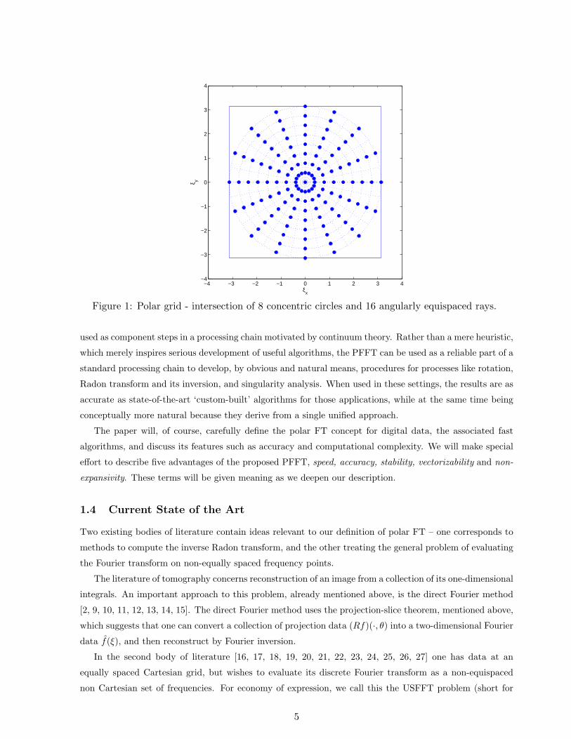
In this paper we propose a notion of a polar FT which is well suited for digital data – a procedure which is
faithful to the continuum polar FT concept, highly accurate, fast, and generally applicable. As in Figure 1
, we define the polar grid of frequencies ξp,q = {ξx[p, q], ξy[p, q]} in the circle inscribed in the fundamental
region ξ ∈ [−π, π)2, and, given digital Cartesian data f [i1, i2] we define the polar FT to be the collection
of samples {F (ξp,q)}, where F (ξ) is the trigonometric polynomial
F (ξp,q) =∑
i1
∑
i2
f [i1, i2] exp (−i1ξx[p, q]− i2ξy[p, q]) .
Thinking of the polar Discrete Fourier Transform (PDFT) mapping PDFT : f [i1, i2] → F (ξp,q) as a linear
operator, we also consider a generalized inverse procedure of it, going back from discrete polar Fourier data
to cartesian spatial data. We define the required density of polar samples in the frequency domain in order
to enable such stable inversion.
This notion of polar FT and its (generalized) inverse leads to a natural and automatic Polar Fast Fourier
Transform (PFFT) algorithm and a natural and automatic inverse PFFT (IPFFT), which can be reliably
4
−4 −3 −2 −1 0 1 2 3 4−4
−3
−2
−1
0
1
2
3
4
ξx
ξ y
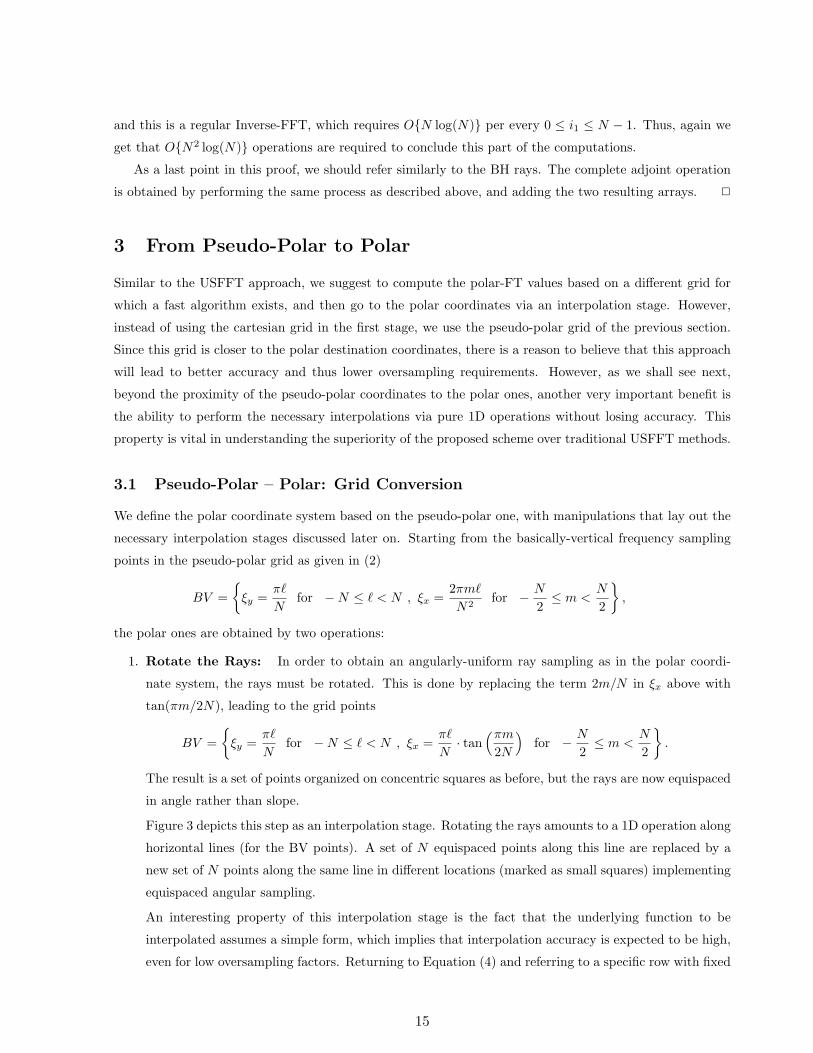
Figure 1: Polar grid - intersection of 8 concentric circles and 16 angularly equispaced rays.
used as component steps in a processing chain motivated by continuum theory. Rather than a mere heuristic,
which merely inspires serious development of useful algorithms, the PFFT can be used as a reliable part of a
standard processing chain to develop, by obvious and natural means, procedures for processes like rotation,
Radon transform and its inversion, and singularity analysis. When used in these settings, the results are as
accurate as state-of-the-art ‘custom-built’ algorithms for those applications, while at the same time being
conceptually more natural because they derive from a single unified approach.
The paper will, of course, carefully define the polar FT concept for digital data, the associated fast
algorithms, and discuss its features such as accuracy and computational complexity. We will make special
effort to describe five advantages of the proposed PFFT, speed, accuracy, stability, vectorizability and non-
expansivity. These terms will be given meaning as we deepen our description.
1.4 Current State of the Art
Two existing bodies of literature contain ideas relevant to our definition of polar FT – one corresponds to
methods to compute the inverse Radon transform, and the other treating the general problem of evaluating
the Fourier transform on non-equally spaced frequency points.
The literature of tomography concerns reconstruction of an image from a collection of its one-dimensional
integrals. An important approach to this problem, already mentioned above, is the direct Fourier method
[2, 9, 10, 11, 12, 13, 14, 15]. The direct Fourier method uses the projection-slice theorem, mentioned above,
which suggests that one can convert a collection of projection data (Rf)(·, θ) into a two-dimensional Fourier
data f(ξ), and then reconstruct by Fourier inversion.
In the second body of literature [16, 17, 18, 19, 20, 21, 22, 23, 24, 25, 26, 27] one has data at an
equally spaced Cartesian grid, but wishes to evaluate its discrete Fourier transform as a non-equispaced
non Cartesian set of frequencies. For economy of expression, we call this the USFFT problem (short for
5
Unequally Spaced Frequency Fourier Transform).
While neither literature explicitly develops a concept of polar FT, it is not hard to see the direct
relevance to the definition we have given. First, we note that the polar sampling set defined above is
certainly a non-equispaced, non-Cartesian set. Thus, the problem of computing F (ξp,q) from digital data
f [i1, i2] is explicitly a problem of evaluating the Fourier transform of f at unequally spaced frequencies. In
other words, the problem of computing the PDFT is a special case of the USFFT problem, though not one
discussed in the above mentioned literature.
Second, note that, if we take the projection data (Rf)(·, θ) and perform a discrete Fourier transform in
the (discretely sampled) t-variable, we effectively have f(ξp,q). Hence, the problem of Radon inversion is
closely connected to the problem of going back from discrete polar Fourier data f(ξp,q) to Cartesian spatial
data f [i1, i2].
In short, it appears that the two literatures concern problems which are inverses of one another. However,
as we shall see later in this section, the approach taken by both is very similar, leaning on oversampling
and two-dimensional interpolation.
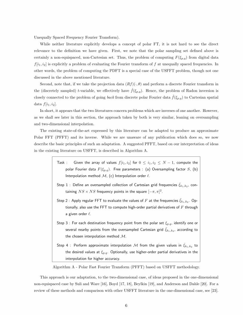
The existing state-of-the-art expressed by this literature can be adapted to produce an approximate
Polar FFT (PFFT) and its inverse. While we are unaware of any publication which does so, we now
describe the basic principles of such an adaptation. A suggested PFFT, based on our interpretation of ideas
in the existing literature on USFFT, is described in Algorithm A.
Task : Given the array of values f [i1, i2] for 0 ≤ i1, i2 ≤ N − 1, compute the
polar Fourier data F (ξp,q). Free parameters : (a) Oversampling factor S, (b)
Interpolation method M, (c) Interpolation order `.
Step 1 : Define an oversampled collection of Cartesian grid frequencies ξk1,k2 , con-
taining NS ×NS frequency points in the square [−π, π]2.
Step 2 : Apply regular FFT to evaluate the values of F at the frequencies ξk1,k2 . Op-
tionally, also use the FFT to compute high-order partial derivatives of F through
a given order `.
Step 3 : For each destination frequency point from the polar set ξp,q, identify one or
several nearby points from the oversampled Cartesian grid ξk1,k2 , according to
the chosen interpolation method M.
Step 4 : Perform approximate interpolation M from the given values in ξk1,k2 to
the desired values at ξp,q. Optionally, use higher-order partial derivatives in the
interpolation for higher accuracy.
Algorithm A - Polar Fast Fourier Transform (PFFT) based on USFFT methodology.
This approach is our adaptation, to the two-dimensional case, of ideas proposed in the one-dimensional
non-equispaced case by Suli and Ware [16], Boyd [17, 18], Beylkin [19], and Anderson and Dahle [20]. For a
review of these methods and comparison with other USFFT literature in the one-dimensional case, see [23].
6
Many variations are possible, but the most important ones concern the choice of degree of oversampling
and the degree of approximation (i.e. degree of accuracy of the approximate interpolation formula).
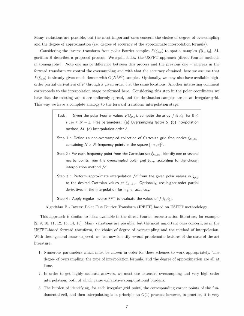
Considering the inverse transform from polar Fourier samples F (ξp,q) to spatial samples f [i1, i2], Al-
gorithm B describes a proposed process. We again follow the USFFT approach (direct Fourier methods
in tomography). Note one major difference between this process and the previous one – whereas in the
forward transform we control the oversampling and with that the accuracy obtained, here we assume that
F (ξp,q) is already given much denser with O(N2S2) samples. Optionally, we may also have available high-
order partial derivatives of F through a given order ` at the same locations. Another interesting comment
corresponds to the interpolation stage performed here. Considering this step in the polar coordinates we
have that the existing values are uniformly spread, and the destination samples are on an irregular grid.
This way we have a complete analogy to the forward transform interpolation stage.
Task : Given the polar Fourier values F (ξp,q), compute the array f [i1, i2] for 0 ≤i1, i2 ≤ N − 1. Free parameters : (a) Oversampling factor S, (b) Interpolation
method M, (c) Interpolation order `.
Step 1 : Define an non-oversampled collection of Cartesian grid frequencies ξk1,k2 ,
containing N ×N frequency points in the square [−π, π]2.
Step 2 : For each frequency point from the Cartesian set ξk1,k2 , identify one or several
nearby points from the oversampled polar grid ξp,q, according to the chosen
interpolation method M.
Step 3 : Perform approximate interpolation M from the given polar values in ξp,q
to the desired Cartesian values at ξk1,k2 . Optionally, use higher-order partial
derivatives in the interpolation for higher accuracy.
Step 4 : Apply regular Inverse FFT to evaluate the values of f [i1, i2].
Algorithm B - Inverse Polar Fast Fourier Transform (IPFFT) based on USFFT methodology.
This approach is similar to ideas available in the direct Fourier reconstruction literature, for example
[2, 9, 10, 11, 12, 13, 14, 15]. Many variations are possible, but the most important ones concern, as in the
USFFT-based forward transform, the choice of degree of oversampling and the method of interpolation.
With these general issues exposed, we can now identify several problematic features of the state-of-the-art
literature:
1. Numerous parameters which must be chosen in order for these schemes to work appropriately. The
degree of oversampling, the type of interpolation formula, and the degree of approximation are all at
issue.
2. In order to get highly accurate answers, we must use extensive oversampling and very high order
interpolation, both of which cause exhaustive computational burdens.
3. The burden of identifying, for each irregular grid point, the corresponding corner points of the fun-
damental cell, and then interpolating is in principle an O(1) process; however, in practice, it is very
7
expensive. In practice, the different corner points, although geometrically close, can be stored very far
apart in linear memory, causing cache misses for a high proportion of interpolation1. Because memory
speed is so much slower than cache speed, the cache misses effectively constrain the overall run time
of the algorithm.
4. The “forward” and “inverse” polar FT’s defined this way need not be inverses of each other. Since the
methods are approximate in each direction, there is no possibility of an exact reconstruction property
– i.e. a reconstruction which is exact modulo the usual arithmetic precision effects associated with
floating-point computations.
In short, there are various uncertainties and complexities associated with an implementation using the
current state-of-the-art ideas from the USFFT and direct Fourier methods in tomography literature.
1.5 The New Approach
The approach we propose for PFFT factors the problem into two steps: first, a pseudo-polar FFT is applied,
in which a pseudo-polar sampling set is used, and second, a conversion from pseudo-polar to polar FT is
performed.
At the heart of the method proposed here for the PFFT we use the pseudo-polar FFT – an FFT where
the evaluation frequencies lie in an oversampled set of non-angularly equispaced points (see Figure 2).
The pseudo-polar FFT offers us a near-polar frequency coordinate system for which exact rapid evaluation
are possible [28]. Whereas the polar grid points sit at the intersection between linearly growing concentric
circles and angularly equispaced rays, the pseudo-polar points sit at the intersection between linearly growing
concentric squares and a specific choice of angularly non-equispaced rays.
The pseudo-polar transform plays the role of a halfway point – a nearly-polar system from which con-
version to Polar Coordinates uses processes relying purely on 1-D FFT’s and interpolation operations.
We present this conversion process, along with an error analysis of it, showing far improved performance
compared to the USFFT-based approach.
As mentioned above, the above described approach enjoys the following important advantages:
• Complexity: For a given two-dimensional signal of size N ×N , the complexity of both the proposed
Polar FFT and its inverse is of order N2 log N , just like in a Cartesian 2D-FFT operating on the same
input array.
• Accuracy: Since polynomial interpolations are involved in the algorithm’s path, exact results cannot
be claimed. However, as will be shown later, the applied interpolations are expected to yield highly
accurate results due to specific features of the frequency domain function slices. The accuracy obtained
is 2 orders of magnitude better than the one expected with the best among the USFFT-based methods.
• Stability: This property refers mostly to our ability to invert the transform, and claim almost one-
to-one mapping between spatial array and its and PFFT result. Two ingredients are responsible for
such a behavior - adequate conditioning of the signal prior to its transform, and a proper set of polar
1This could be analyzed leading to a quantitative evaluation of the cache miss rate.
8

frequency samples that would be considered representative. We show how those two considerations
lead to traceable process with stable inversion.
• Vectorizability: The process we propose is organized as a series of purely one-dimensional signal
manipulation processes, in which data form a single row or column of an array are subjected to
a series of Fourier transforms, 1D interpolations, and ancillary operations. Owing to the use of
vectorized operations, there are effectively very few cache misses in any component step. Moreover,
since many of the involved operations are 1D-FFT, there are opportunities on modern consumer PC
architecture – such as PowerPC G4 chips – to use fast in silicon FFT algorithms operating at speeds
far higher than the usual assembly-coded routines.
• Non-expansivity: There is no drastic oversampling of the underlying array. If we recall the USFFT
approach described earlier, it turns out that very substantial degrees of oversampling are necessary to
get high accuracy. The transformation we describe here is oversampled by factor 2 in each coordinate
and yet is essentially exact.
1.6 Content
This paper is organized as follows:
• Section 2 describes the pseudo-polar Fourier grid, the forward and inverse transform with this grid.
In this section we closely follow the work in [28].
• Section 3 then discusses the conversion from pseudo-polar – to –polar for the forward transform,
and from polar – to – pseudo-polar in the inverse one. We show how these conversions amount
to one-dimensional operations, and discuss reasons for the high interpolation accuracy obtained. A
pre-process stage is introduced in order to guarantee stability of the forward and inverse transforms.
• Section 4 analyzes the proposed algorithm from several aspects. Accuracy is studied by bounding the
interpolation error and by finding the worst-case scenarios maximizing the approximation error.
• Section 5 gives a brief description of a freely available software performing the forward and inverse
transform from Cartesian spatial domain to polar frequency and backwards to the spatial domain.
This software also includes the code to reproduce this paper’s results.
• Section 6 concludes this paper, with discussion on future work and open questions.
2 Pseudo-Polar Fourier Transform
The pseudo-polar Fourier transform is based on a definition of a polar-like 2D grid that enables fast Fourier
computation. This grid has been explored by many since the 1970-s. The pioneers in this field are Mersereau
and Oppenheim [30] who proposed the concentric squares grid as an alternative to the polar grid. Work by
Pasciak [31], Edholm and Herman [32], and Lawton [33] showed that fast exact evaluation on such grids is
possible. Later work by Munson and others [12, 13] have shown how these ideas can be extended and used
9
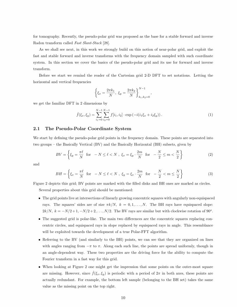
for tomography. Recently, the pseudo-polar grid was proposed as the base for a stable forward and inverse
Radon transform called Fast Slant-Stack [28].
As we shall see next, in this work we strongly build on this notion of near-polar grid, and exploit the
fast and stable forward and inverse transforms with the frequency domain sampled with such coordinate
system. In this section we cover the basics of the pseudo-polar grid and its use for forward and inverse
transform.
Before we start we remind the reader of the Cartesian grid 2-D DFT to set notations. Letting the
horizontal and vertical frequencies{
ξx =2πk1
N, ξy =
2πk2
N
}N−1
k1,k2=0
,
we get the familiar DFT in 2 dimensions by
f(ξx, ξy) =N−1∑
i1=0
N−1∑
i2=0
f [i1, i2] · exp (−i(i1ξx + i2ξy)) . (1)
2.1 The Pseudo-Polar Coordinate System
We start by defining the pseudo-polar grid points in the frequency domain. These points are separated into
two groups – the Basically Vertical (BV) and the Basically Horizontal (BH) subsets, given by
BV ={
ξy =π`
Nfor −N ≤ ` < N , ξx = ξy · 2m
Nfor − N
2≤ m <
N
2
}(2)
and
BH ={
ξx =π`
Nfor −N ≤ ` < N , ξy = ξx · 2m
Nfor − N
2< m ≤ N
2
}(3)
Figure 2 depicts this grid; BV points are marked with the filled disks and BH ones are marked as circles.
Several properties about this grid should be mentioned:
• The grid points live at intersections of linearly growing concentric squares with angularly non-equispaced
rays. The squares’ sides are of size πk/N, k = 0, 1, . . . , N . The BH rays have equispaced slope:
2k/N, k = −N/2+1,−N/2+2, . . . , N/2. The BV rays are similar but with clockwise rotation of 90o.
• The suggested grid is polar-like. The main two differences are the concentric squares replacing con-
centric circles, and equispaced rays in slope replaced by equispaced rays in angle. This resemblance
will be exploited towards the development of a true Polar-FFT algorithm.
• Referring to the BV (and similarly to the BH) points, we can see that they are organized on lines
with angles ranging from −π to π. Along each such line, the points are spread uniformly, though in
an angle-dependent way. These two properties are the driving force for the ability to compute the
Fourier transform in a fast way for this grid.
• When looking at Figure 2 one might get the impression that some points on the outer-most square
are missing. However, since f(ξx, ξy) is periodic with a period of 2π in both axes, these points are
actually redundant. For example, the bottom left sample (belonging to the BH set) takes the same
value as the missing point on the top right.
10
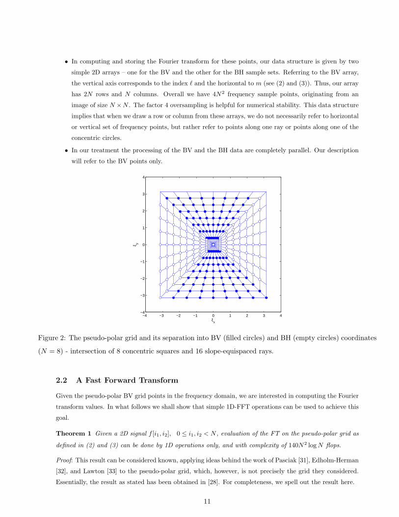
• In computing and storing the Fourier transform for these points, our data structure is given by two
simple 2D arrays – one for the BV and the other for the BH sample sets. Referring to the BV array,
the vertical axis corresponds to the index ` and the horizontal to m (see (2) and (3)). Thus, our array
has 2N rows and N columns. Overall we have 4N2 frequency sample points, originating from an
image of size N ×N . The factor 4 oversampling is helpful for numerical stability. This data structure
implies that when we draw a row or column from these arrays, we do not necessarily refer to horizontal
or vertical set of frequency points, but rather refer to points along one ray or points along one of the
concentric circles.
• In our treatment the processing of the BV and the BH data are completely parallel. Our description
will refer to the BV points only.
−4 −3 −2 −1 0 1 2 3 4−4
−3
−2
−1
0
1
2
3
4
ξx
ξ y
Figure 2: The pseudo-polar grid and its separation into BV (filled circles) and BH (empty circles) coordinates
(N = 8) - intersection of 8 concentric squares and 16 slope-equispaced rays.
2.2 A Fast Forward Transform
Given the pseudo-polar BV grid points in the frequency domain, we are interested in computing the Fourier
transform values. In what follows we shall show that simple 1D-FFT operations can be used to achieve this
goal.
Theorem 1 Given a 2D signal f [i1, i2], 0 ≤ i1, i2 < N , evaluation of the FT on the pseudo-polar grid as
defined in (2) and (3) can be done by 1D operations only, and with complexity of 140N2 log N flops.
Proof: This result can be considered known, applying ideas behind the work of Pasciak [31], Edholm-Herman
[32], and Lawton [33] to the pseudo-polar grid, which, however, is not precisely the grid they considered.
Essentially, the result as stated has been obtained in [28]. For completeness, we spell out the result here.
11

Using the definition of the Fourier transform for discrete functions in Equation (1), and plugging the
coordinates from Equation (2) and (3) we obtain
f(ξx, ξy) = f [m, `] =N−1∑
i1=0
N−1∑
i2=0
f [i1, i2] · exp (−i(i1ξx + i2ξy)) (4)
=N−1∑
i1=0
N−1∑
i2=0
f [i1, i2] · exp(−i
(2πi1`m
N2+
πi2`
N
))
=N−1∑
i1=0
exp(− i2πi1`m
N2
) N−1∑
i2=0
f [i1, i2] · exp(− iπi2`
N
).
Concentrating on the inner summation part, we define
f1[i1, `] =N−1∑
i2=0
f [i1, i2] · exp(− iπi2`
N
). (5)
This expression stands for a 1D-FFT on the columns of the zero padded array f [i1, i2]. In order to show
this, assume that f [i1, i2] is zero padded to yield
fZ [i1, i2] =
f [i1, i2] 0 ≤ i2 < N
0 N ≤ i2 < 2N
Thus,
f1[i1, `] =N−1∑
i2=0
f [i1, i2] · exp(− iπi2`
N
)=
2N−1∑
i2=0
fZ [i1, i2] · exp(− i2πi2`
2N
). (6)
This expression stands for 1D-FFT of an array of 2N samples. However, another complicating factor is
the range of ` (−N ≤ ` ≤ N − 1), as opposed to the regular FFT range that starts at 0. Thus, defining
n = ` + N we get
f1[i1, n] =2N−1∑
i2=0
fZ [i1, i2] · exp(− i2πi2(n−N)
2N
)(7)
=2N−1∑
i2=0
fZ [i1, i2] · (−1)i2 · exp(− i2πi2n
2N
).
To summarize this part, we found that computation of the inner summation (w.r.t. i2) amounts to 1D-FFT
of length 2N on the columns of the zero padded and pre-multiplied2 array f [i1, i2] · (−1)i2 . The amount of
operations needed for this stage are 5 · 2N log(2N) per each column, and 10N2 log(2N) operations for all
the N columns.
We return now to Equation (4), and assume that the above process has been completed. Thus we hold
the N × 2N array f1[i1, `], and we should proceed by computing the second summation
f [m, `] =N−1∑
i1=0
f1[i1, `] exp(− i2πi1m`
N2
)=
N−1∑
i1=0
f1[i1, `] exp(− i2πi1m
N· `
N
). (8)
2We have to multiply our array by (−1)i2 , but this could be replaced by later shift, owing to the periodic nature of the
transform.
12
Removal of the factor α = `/N in the exponent turns this expression into a regular 1D-FFT, this time
applied on the rows of the array f1. With this factor α in the above summation, the required operation is
known as the Chirp-Z [35], or the Fractional Fourier Transform (FRFT) [36]. In Appendix A we show how
this transform can be computed efficiently for any α, with 30N log N operations, based on 1D-FFT use. As
before, due to a shifted range of the index m, one has either to shift after the transform, or modulate the
array, prior to the transform.
To summarize, we have 2N rows that are to be put through a Chirp-Z transform. Thus we need
60N2 log N operations for this stage. Adding to the previous stage complexity, we get an overall of
70N2 log N operations for the computation of the transform for the BV part of the grid. To cover both the
BV and the BH grid points we need 140N2 log N . 2
In this paper the pseudo-polar grid is a stepping stone towards the polar coordinates system. Interpo-
lations will be made to convert from pseudo-polar to polar coordinates. For better interpolation results, we
consider computing the pseudo-polar FFT for more densely-spaced grid. We state here two results showing
how the pseudo-polar FFT works for an oversampled grid.
Theorem 2 Given a 2D signal f [i1, i2], 0 ≤ i1, i2 < N , the evaluation of the FT on the oversampled
pseudo-polar grid with NS concentric squares and 2NP slope-equispaced rays can be obtained by 1D vector
operations only, and with complexity of 120N2PS log(NS) flops.
Conceptually, this result follows immediately from Theorem 1 with zero-padding. Here we state this
result. For simplicity we assume P = S.
Theorem 3 Given a 2D signal f [i1, i2], 0 ≤ i1, i2 < N , the evaluation of the FT on the oversampled
pseudo-polar grid with NS concentric squares and 2NS rays can be done by applying the regular pseudo-
polar FFT on the signal
fZ [i1, i2] =
f [i1, i2] 0 ≤ i1, i2 < N
0 N ≤ i2 < SN or N ≤ i2 < SN. (9)
2.3 Fast Inverse Transform and Quasi-Parseval Relationship
The pseudo-polar FFT can be inverted by the method of Least-Squares (LS). To see this, consider a matrix-
vector formulation of our processes. For an image f [i1, i2] of size N × N , we define the column vector f
of length N2, containing the image pixel values in column-stack ordering. This vector is multiplied by a
matrix TPP ∈ C4N2×N2, representing the pseudo-polar FFT. The outcome of this multiplication is a vector
f of length 4N2, containing the samples of the Fourier transform on the pseudo-polar grid.
Given f , inversion of the pseudo-polar Fourier transform is achieved by solving
f = Arg minx
∥∥∥TPP x− f∥∥∥
2
2=
(TH
PP TPP
)−1TH
PP f = T+PP f . (10)
where T+PP denotes generalized inverse.
Of course, the matrix-based solution is useless as a computational approach for reasonable sizes of
input arrays; a pseudo direct inversion of the matrix TPP is computationally prohibitive, and definitely
13
beyond the desired N2 log(N) complexity. Instead, we approach the optimization problem iteratively by
the iteration relation
fk+1
= fk−DTH
PP
(TPP f
k− f
). (11)
The expression THPP
(TPP x− f
)is the function’s gradient, and the multiplication by a positive definite
matrix D guarantees descent in the LS error. If chosen properly, D could speed-up convergence of this
algorithm to the true solution, as posed in (10). In [28] a specific choice of diagonal matrix D is proposed
that down-weights near-origin points in order to equalize the condition number. It is shown that with few
(2 − 6) iterations this iterative process achieves high accuracy solutions. As to the initialization, it could
be chosen as zeros for simplicity.
This way we obtain a fast inverse transform of the same complexity as the forward one, as every iteration
requires the application of both the forward transform (multiplying with TPP ) and its adjoint (multiplying
with THPP ). It still remains to be seen that the adjoint is computable with the same complexity as the
forward transform, which is the claim of the next Theorem.
Theorem 4 Given a 2D array f [m, `] of size 2N × 2N representing a pseudo-polar grid sampling in the
frequency domain, the evaluation of the adjoint pseudo-polar FFT to produce an N ×N image can be done
by 1D operations only, and with complexity of O{N2 log(N)} operations.
Proof: Posed in a matrix notation, multiplication by THPP requires taking the conjugate of each element in
the matrix TPP , and summing with respect to columns, rather than rows. Thus, using the relation posed
in (4) we have that the regular (forward) transform is applied by
f [m, `] =N−1∑
i1=0
N−1∑
i2=0
f [i1, i2] · exp(−i
(2πi1`m
N2+
πi2`
N
)).
Similarly, referring to the basically vertical (BV) values only, the adjoint is achieved by
f [i1, i2] =N/2−1∑
m=−N/2
N−1∑
`=−N
f [m, `] · exp(
i
(2πi1`m
N2+
πi2`
N
))(12)
=N−1∑
`=−N
exp(
iπi2`
N
) N/2−1∑
m=−N/2
f [m, `] · exp(
i2πi1`m
N2
).
The inner summation could be written as
f [i1, `] =N/2−1∑
m=−N/2
f [m, `] · exp(
i2πi1m
N· `
N
),
and this is a Fractional FFT, just as we obtained with the forward transform. We have seen that this
operation could be done in O{N log(N)} per every `, producing N values. Thus, for −N ≤ ` ≤ N − 1 we
need to perform O{N2 log(N)} operations. Once performed, we then obtain the expression
f [i1, i2] =N−1∑
`=−N
exp(
iπi2`
N
)f [i1, `], (13)
14
and this is a regular Inverse-FFT, which requires O{N log(N)} per every 0 ≤ i1 ≤ N − 1. Thus, again we
get that O{N2 log(N)} operations are required to conclude this part of the computations.
As a last point in this proof, we should refer similarly to the BH rays. The complete adjoint operation
is obtained by performing the same process as described above, and adding the two resulting arrays. 2
3 From Pseudo-Polar to Polar
Similar to the USFFT approach, we suggest to compute the polar-FT values based on a different grid for
which a fast algorithm exists, and then go to the polar coordinates via an interpolation stage. However,
instead of using the cartesian grid in the first stage, we use the pseudo-polar grid of the previous section.
Since this grid is closer to the polar destination coordinates, there is a reason to believe that this approach
will lead to better accuracy and thus lower oversampling requirements. However, as we shall see next,
beyond the proximity of the pseudo-polar coordinates to the polar ones, another very important benefit is
the ability to perform the necessary interpolations via pure 1D operations without losing accuracy. This
property is vital in understanding the superiority of the proposed scheme over traditional USFFT methods.
3.1 Pseudo-Polar – Polar: Grid Conversion
We define the polar coordinate system based on the pseudo-polar one, with manipulations that lay out the
necessary interpolation stages discussed later on. Starting from the basically-vertical frequency sampling
points in the pseudo-polar grid as given in (2)
BV ={
ξy =π`
Nfor −N ≤ ` < N , ξx =
2πm`
N2for − N
2≤ m <
N
2
},
the polar ones are obtained by two operations:
1. Rotate the Rays: In order to obtain an angularly-uniform ray sampling as in the polar coordi-
nate system, the rays must be rotated. This is done by replacing the term 2m/N in ξx above with
tan(πm/2N), leading to the grid points
BV ={
ξy =π`
Nfor −N ≤ ` < N , ξx =
π`
N· tan
(πm
2N
)for − N
2≤ m <
N
2
}.
The result is a set of points organized on concentric squares as before, but the rays are now equispaced
in angle rather than slope.
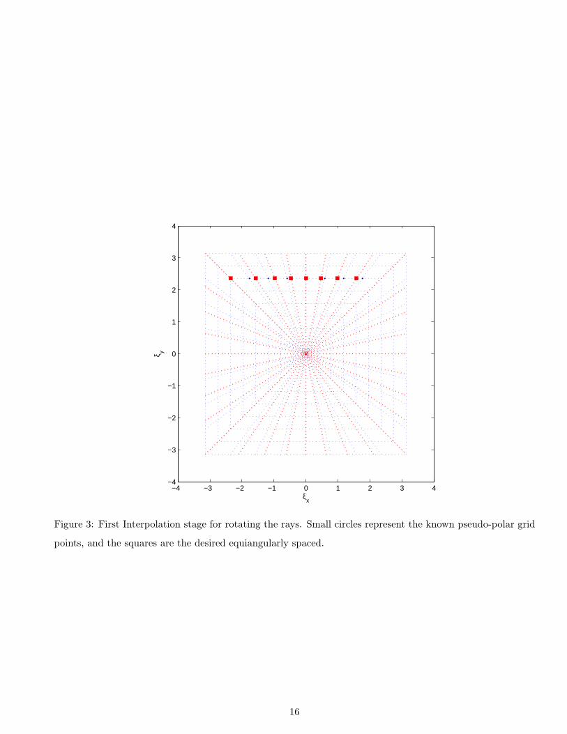
Figure 3 depicts this step as an interpolation stage. Rotating the rays amounts to a 1D operation along
horizontal lines (for the BV points). A set of N equispaced points along this line are replaced by a
new set of N points along the same line in different locations (marked as small squares) implementing
equispaced angular sampling.
An interesting property of this interpolation stage is the fact that the underlying function to be
interpolated assumes a simple form, which implies that interpolation accuracy is expected to be high,
even for low oversampling factors. Returning to Equation (4) and referring to a specific row with fixed
15
−4 −3 −2 −1 0 1 2 3 4−4
−3
−2
−1
0
1
2
3
4
ξx
ξ y
Figure 3: First Interpolation stage for rotating the rays. Small circles represent the known pseudo-polar grid
points, and the squares are the desired equiangularly spaced.
16
ξy, we have
f(m, ξy) =N−1∑
i1=0
N−1∑
i2=0
f [i1, i2] · exp(−i
[2mi1N
+ i2
]ξy
)
=N−1∑
i1=0
[N−1∑
i2=0
exp (−iξyi2) f [i1, i2]
]· exp
(−i
2mi1N
ξy
)(14)
=N−1∑
i1=0
C[i1] ·[exp
(−i
2i1N
ξy
)]m
and this is a complex trigonometric polynomial of order N .
One implication of this observation is that given N samples of this function, all information about
this function is given. Theoretically, this implies that a perfect interpolation is possible if for every
destination points all the N given samples are used. From a more practical point of view, the above
observation implies that this function is relatively smooth and with a moderate oversampling (factor
of 2− 4) a near-perfect interpolation is expected for a small neighborhood operation.
2. Circle the Squares: In order to obtain concentric circles as required in the polar coordinate system,
we need to ‘circle the squares’. This is done by dividing both ξx and ξy by a constant along each ray,
based on its angle, and therefore a function of the parameter m, being
R[m] =√
1 + tan2(πm
2N
)(15)
The resulting grid is given by
BV =
ξy = π`NR[m] for −N ≤ ` < N
ξx = π`NR[m] · tan
(πm2N
)for − N
2 ≤ m < N2
.
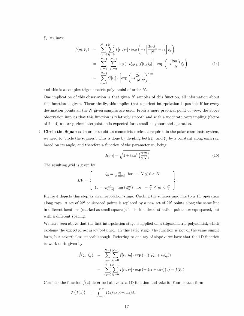
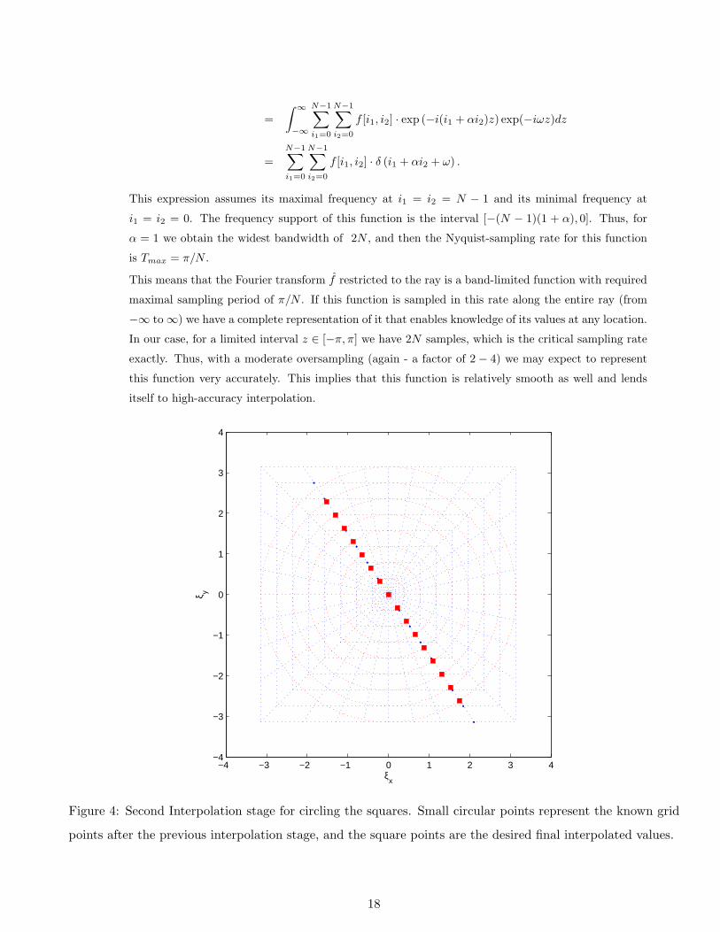
Figure 4 depicts this step as an interpolation stage. Circling the squares amounts to a 1D operation
along rays. A set of 2N equispaced points is replaced by a new set of 2N points along the same line
in different locations (marked as small squares). This time the destination points are equispaced, but
with a different spacing.
We have seen above that the first interpolation stage is applied on a trigonometric polynomial, which
explains the expected accuracy obtained. In this later stage, the function is not of the same simple
form, but nevertheless smooth enough. Referring to one ray of slope α we have that the 1D function
to work on is given by
f(ξx, ξy) =N−1∑
i1=0
N−1∑
i2=0
f [i1, i2] · exp (−i(i1ξx + i2ξy))
=N−1∑
i1=0
N−1∑
i2=0
f [i1, i2] · exp (−i(i1 + αi2)ξx) = f(ξx)
Consider the function f(z) described above as a 1D function and take its Fourier transform
F{f(z)} =∫ ∞
−∞f(z) exp(−iωz)dz
17
=∫ ∞
−∞
N−1∑
i1=0
N−1∑
i2=0
f [i1, i2] · exp (−i(i1 + αi2)z) exp(−iωz)dz
=N−1∑
i1=0
N−1∑
i2=0
f [i1, i2] · δ (i1 + αi2 + ω) .
This expression assumes its maximal frequency at i1 = i2 = N − 1 and its minimal frequency at
i1 = i2 = 0. The frequency support of this function is the interval [−(N − 1)(1 + α), 0]. Thus, for
α = 1 we obtain the widest bandwidth of 2N , and then the Nyquist-sampling rate for this function
is Tmax = π/N .
This means that the Fourier transform f restricted to the ray is a band-limited function with required
maximal sampling period of π/N . If this function is sampled in this rate along the entire ray (from
−∞ to ∞) we have a complete representation of it that enables knowledge of its values at any location.
In our case, for a limited interval z ∈ [−π, π] we have 2N samples, which is the critical sampling rate
exactly. Thus, with a moderate oversampling (again - a factor of 2 − 4) we may expect to represent
this function very accurately. This implies that this function is relatively smooth as well and lends
itself to high-accuracy interpolation.
−4 −3 −2 −1 0 1 2 3 4−4
−3
−2
−1
0
1
2
3
4
ξx
ξ y
Figure 4: Second Interpolation stage for circling the squares. Small circular points represent the known grid
points after the previous interpolation stage, and the square points are the desired final interpolated values.
18

In performing the polar-FFT, we start with computation of the Fourier transform over a pseudo-polar
grid, followed by the two interpolation stages presented above. As we have seen, in order to obtain high
accuracy, the pseudo-polar grid must be oversampled, both radially and angularly. One approach to over-
sampling is the use of the over-complete pseudo-polar grid as presented in the previous section. Alternatively,
as the pseudo-polar fast transform can be broken into two parts, this separation could be used for better
efficiency. For the BV coordinates, the vertical FFT can be done with oversampling by zero padding as
before, and then, as we go to the second phase of Fractional FFT per each row, we can apply this stage
one row at a time with the interpolation that leads directly to the rotated rays. The memory savings are
substantial (directly proportional to the oversampling factor P ). Note that in performing the 1D interpola-
tions, complete rows or columns from the result array are brought to the cache, and processed to produce
the desired values. Thus, memory management becomes extremely effective, as opposed to the regular
USFFT methods that require general memory access and lead to many cache misses.
As for the complexity of the overall algorithm, we have seen before that an amount of 120N2SP log2(NS)
operations are required for the computation of the oversampled pseudo-polar FFT. Those operations are
followed by the first interpolation requiring O(N2S) operations (every row uses NP points to compute N
values requires O(N) operations, and there are NS of those). The second interpolation requires O(N2)
operations (every ray with 2NS values is used to produce 2N new values, and there are N rays). Thus, the
overall operation count is dominated by the 120N2SP log2(NS) operations of the pseudo-polar FFT.
In terms of memory requirements, the overcomplete pseudo-polar FFT requires 4N2SP float-values, and
once those are allocated, all other operations can be done within this array. Alternatively, using row-wise
interpolation, only 4N2S values are required. Also, a factor 2 saving can be obtained if a proper separation
between the basically vertical and basically horizontal parts is applied. Further savings could be obtained
by breaking each of these groups (BV and BH) to sub-parts with small overlap.
The inversion of the polar-FFT requires an implementation of the inverse pseudo-polar FFT as described
in the previous section. Starting with a set of polar coordinates in the frequency domain, we first apply
two interpolation stages - squaring the circles, and then rotating the rays - just as described above but in
reverse order. For such operation to succeed, we assume that the polar grid is given in an over-complete
manner (i.e., we start with an array of 2NP [rays] × 2NS[cirlces] and interpolate to a pseudo-polar grid
with 2N [rays]× 2N [squares]). Once those coordinates are filled with values, inverse pseudo-polar FFT is
applied as described previously, using the adjoint operator. The same arguments posed above explain the
suitability of the 1D interpolation and their expected accuracy in the above reverse process.
3.2 Disk Band-Limited Support As Regularization
A major difficulty in using the polar coordinate system with digitally sampled data arises from the square
shape of the fundamental domain [−π, +π]2. In our polar FFT the corners are not represented, and this may
lead to some loss of information. From an algebraic point of view, one may say that the matrix representing
the polar FFT we have defined is not invertible, or badly conditioned.
A way around this problem is to assume that there is no vanishing content in those non-sampled corners.
This means that the image should be supported in the frequency domain inside a disk of radius π, leaving
19

the corners empty. If the given image is sampled at√
2 times the Nyquist rate on both cartesian axes then
it’s frequency domain support is the square [−π/√
2,+π/√
2]2, and this square is contained in the disk
required. Figure 5 presents these support regions in the frequency domain. Thus, given any image, we can
easily verify that this condition holds: zero-padding the image by factor√
2 in both axes, and applying
2D-FFT followed by 2D-IFFT, the result image is twice as big (in pixel count) and its frequency domain
support is as required. All these operations add O(N2 log2(N) flops to the polar FFT that follows.
−4 −3 −2 −1 0 1 2 3 4−4
−3
−2
−1
0
1
2
3
4
ξx
ξ y
Figure 5: Frequency domain: The fundamental domain [−π, +π]2, its inscribed circle of radius π, and the
square inscribed in this circle, [−π/√
2, +π/√
2]2.
In the inversion transform from the frequency polar-coordinates to the spatial domain, the knowledge
about the corners having zero content is valuable, and could be used to further stabilize the inverse trans-
form. This is done in the interpolation to the pseudo-polar grid, by assigning zero values to all grid-points
outside the π-radius circle3 .
Figure 6 presents the effect of the corner-nulling process proposed here on the condition number of the
transform matrix. For an input array of size N × N (with N assuming the values 4, 6, 8, . . . , 30) we
compose the transform matrix for the 4N2 polar coordinates and compute its condition number. As can
be seen from the graph, this value grows exponentially. As an example, for a moderate size of 30 × 30
input array, the condition number is 2e9, implying that inversion by Least-Squares will require numerous
iterations, and will be highly sensitive to numerical errors.
The second curve refers to the same transform matrix with an augmented part referring to the corners.
The augmentation part is generated by generating a regular 4N × 4N cartesian grid transform matrix, and
choosing the rows that refer to the corner (outside the π-radius disk). Roughly speaking, we have doubled
3Note that this discussion is not to be confused with the need to apply preconditioning in the inversion of the pseudo-polar
transform.
20
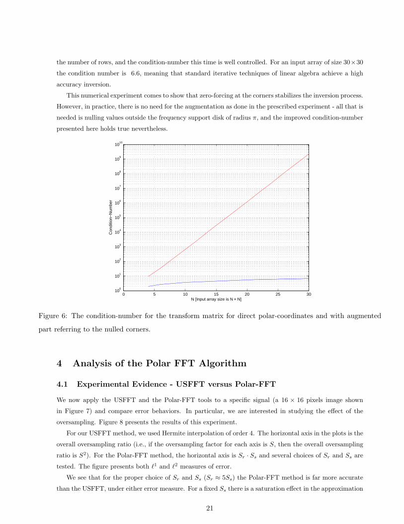
the number of rows, and the condition-number this time is well controlled. For an input array of size 30×30
the condition number is 6.6, meaning that standard iterative techniques of linear algebra achieve a high
accuracy inversion.
This numerical experiment comes to show that zero-forcing at the corners stabilizes the inversion process.
However, in practice, there is no need for the augmentation as done in the prescribed experiment - all that is
needed is nulling values outside the frequency support disk of radius π, and the improved condition-number
presented here holds true nevertheless.
0 5 10 15 20 25 3010
0
101
102
103
104
105
106
107
108
109
1010
N [Input array size is N × N]
Con
ditio
n−N
umbe
r
Figure 6: The condition-number for the transform matrix for direct polar-coordinates and with augmented
part referring to the nulled corners.
4 Analysis of the Polar FFT Algorithm
4.1 Experimental Evidence - USFFT versus Polar-FFT
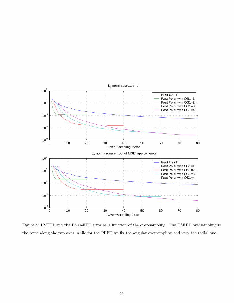
We now apply the USFFT and the Polar-FFT tools to a specific signal (a 16 × 16 pixels image shown
in Figure 7) and compare error behaviors. In particular, we are interested in studying the effect of the
oversampling. Figure 8 presents the results of this experiment.
For our USFFT method, we used Hermite interpolation of order 4. The horizontal axis in the plots is the
overall oversampling ratio (i.e., if the oversampling factor for each axis is S, then the overall oversampling
ratio is S2). For the Polar-FFT method, the horizontal axis is Sr · Ss and several choices of Sr and Ss are
tested. The figure presents both `1 and `2 measures of error.
We see that for the proper choice of Sr and Ss (Sr ≈ 5Ss) the Polar-FFT method is far more accurate
than the USFFT, under either error measure. For a fixed Ss there is a saturation effect in the approximation
21

error as Sr →∞ because errors caused by the first interpolation stage dominate.
The higher needed oversampling along the rays can be explained in two ways: (i) the radial interpolation
stage of the PFFT uses a lower-order procedure, based on splines instead of Hermite; and (ii) the radial
interpolation task is more difficult as the signal to be interpolated is less smooth (see previous Section).
Extensive experiments with different signals, their sizes, and metrics of error evaluations, all confirm
that the above conclusions comparing the USFFT to the Polar-FFT are typical.
2 4 6 8 10 12 14 16
2
4
6
8
10
12
14
160
0.1
0.2
0.3
0.4
0.5
0.6
0.7
0.8
0.9
1
Figure 7: The test image (16× 16).
4.2 Frequency Domain Spread of the Error
Given the specific signal and fixing the oversampling ratio, we study how the errors of the two methods
behave in the frequency domain. Intuitively, we know that USFFT method should cause higher errors
near the origin where the interpolation starts from an inherently coarser grid. In contrast, we expect the
Polar-FFT to perform well near the origin as the accuracy there is high, both because the pseudo-polar
grid supplies exact high density sampling there, and because the interpolation performed near the origin is
of high accuracy as well due to the denser sampling.
Figure 9 show the test image from the previous experiment, its exact polar Fourier transform using the
definition, the errors obtained by the USFFT (S = 9 in both axes), and the Polar-FFT (Sr = 20, Ss = 4).
All the plots show absolute values, and the frequency domain is presented on Cartesian axes in order to give
more intuitive frequency-content description. Since the frequency domain is sampled in polar coordinates
in the transforms, we use a Voronoi diagram to slice the plane into pieces per each polar frequency sample.
This is a matter only of visual display.
Our expectations about the distribution of errors in the frequency domain are validated - the USFFT
concentrates the error at the origin, while the Polar-FFT errors are concentrated near the corners. Moreover,
the errors obtained by the Polar-FFT are better by more than 2 orders of magnitudes.
22
0 10 20 30 40 50 60 70 8010
−6
10−4
10−2
100
102
L1 norm approx. error
Over−Sampling factor
Best USFTFast Polar with OS1=1Fast Polar with OS1=2Fast Polar with OS1=3Fast Polar with OS1=4
0 10 20 30 40 50 60 70 8010
−6
10−4
10−2
100
102
L2 norm (square−root of MSE) approx. error
Over−Sampling factor
Best USFTFast Polar with OS1=1Fast Polar with OS1=2Fast Polar with OS1=3Fast Polar with OS1=4
Figure 8: USFFT and the Polar-FFT error as a function of the over-sampling. The USFFT oversampling is
the same along the two axes, while for the PFFT we fix the angular oversampling and vary the radial one.
23

The test image
5 10 15
2
4
6
8
10
12
14
16 0
0.2
0.4
0.6
0.8
1The exact Fourier transform
10
20
30
40
50
60
Error: USFFT vs. the exact
0
0.005
0.01
0.015
0.02
0.025
Error: New method vs. exact
2
4
6
8
10x 10
−5
Figure 9: The error as a function of frequency location: using a specific signal. This figure shows the original
image (top left), its true PFFT (top right), the error obtained by the USFFT method (bottom left), and the
PFFT algorithm errors (botom right).
4.3 Frequency Domain Spread of the Error - Worst-Case Analysis
A limitation of the above experiment is that it relies on a specific choice of a signal. We now address the
same question from a worst-case point of view: for a specific frequency location in the destination polar
grid, what is the worst possible signal, maximizing the error at this point, and how big is this maximum
error? Answering these questions per each location, we can draw a worst-case error map in the frequency
domain and compare for both the USFFT and the Polar-FFT methods.
Let x of size N ×N denote the signal to be transformed. The transform result has 2N rays containing
2N samples each. As all the involved operations are linear, we adopt a matrix-vector representation for
the exact (Te), the USFFT (Tu) and the Polar-FFT (Tp). All these matrices are of size 4N2 × N2. For
the given signal x of length N2 (due to its lexicographic ordering), the transform error for the USFFT is
(Te −Tu)x, with a similar expression for the Polar-FFT method. To maximize this error is to solve
maxx
‖W (Te −Tu) x‖22‖x‖22
. (16)
W is a diagonal matrix with all entries being zero apart from the one element chosen in the frequency
domain. Thus, essentially, only one row of the matrix Te − Tu is used - denote this as eT . Clearly, by
Cauchy’s inequality, the maximum is obtained for x = e, and the error obtained is ‖e‖2.Figure 10 presents these worst-case errors4 as a function of frequency for both methods when N = 16.
The Polar-FFT performs far better in all locations by 2 orders of magnitude, the Polar-FFT errors are
4In this and later experiments based on the matrix-vector representation of the transforms, we use low value for N because of
the induced matrix sizes. One can use much higher N values if instead of explicitly forming the matrices, the transform and its
adjoint operator are applied within the Power-method. We leave such approach for later work.
24

largest near the boundaries of the frequency support [−π, π]2, while those of the USFFT are large near the
origin. Note that our relatively low choice of N = 16 in this experiment causes special sampling effects.
Worst Error: USFFT vs. the exact
0
0.002
0.004
0.006
0.008
0.01
0.012
Worst Error: New method vs. exact
0
1
2
3
4
5
6
7
8x 10
−4
Figure 10: The error as a function of frequency location: using the worst case signal per location.
4.4 Worst Case Error via Eigenspace Analysis
4.4.1 Direct Approach
Returning to the experiment described in Figure 8, we plot the worst case `2 error of each method under a
fixed oversampling. Using matrix-vector notation, for a given signal x, the transform error of the USFFT
is (Te −Tu)x. Now we solve the optimization problem
maxx
‖(Te −Tu) x‖22‖x‖22
, (17)
seeking the worst-possible signal x maximizing error, subject to unit `2-norm. The answer is of-course the
first right singular vector of (Te −Tu) [34], and the value of (17) is the square of the first singular value5.
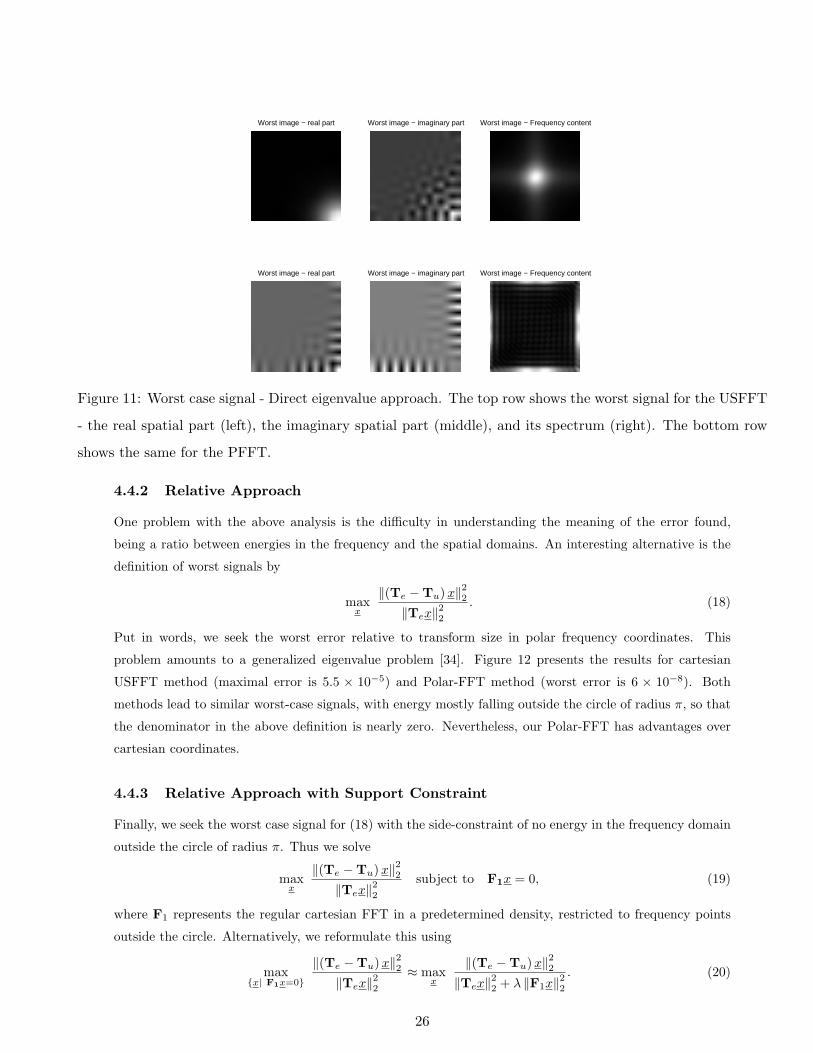
Figure 11 presents the real and imaginary parts of these worst-case signals for the USFFT (S = 9) and
the Polar-FFT (Sr = 20, Ss = 4), and the absolute frequency description of this signal. The USFFT’s
maximal error is 8.9×10⁻³ while the Polar-FFT’s is 1.92×10⁻⁶. Again, the USFFT method is weaker, and
its worst signal is concentrated near the frequency origin where the method is weakest. Note that the worst
signal is modulated (notice the shift from the center in the spatial domain) to result in a very non-smooth
frequency behavior.
5Note that this time the error is MSE and not square-root MSE as in Figure 8 - Thus, while the worst case error in the Polar
FFT method for the oversampling used is 1.92× 10⁻⁶, the specific signal chosen in the construction of figure 8 gives an error of
1× 10⁻¹⁰.
25
Worst image − real part Worst image − imaginary part Worst image − Frequency content
Worst image − real part Worst image − imaginary part Worst image − Frequency content
Figure 11: Worst case signal - Direct eigenvalue approach. The top row shows the worst signal for the USFFT
- the real spatial part (left), the imaginary spatial part (middle), and its spectrum (right). The bottom row
shows the same for the PFFT.
4.4.2 Relative Approach
One problem with the above analysis is the difficulty in understanding the meaning of the error found,
being a ratio between energies in the frequency and the spatial domains. An interesting alternative is the
definition of worst signals by
maxx
‖(Te −Tu) x‖22‖Tex‖22
. (18)
Put in words, we seek the worst error relative to transform size in polar frequency coordinates. This
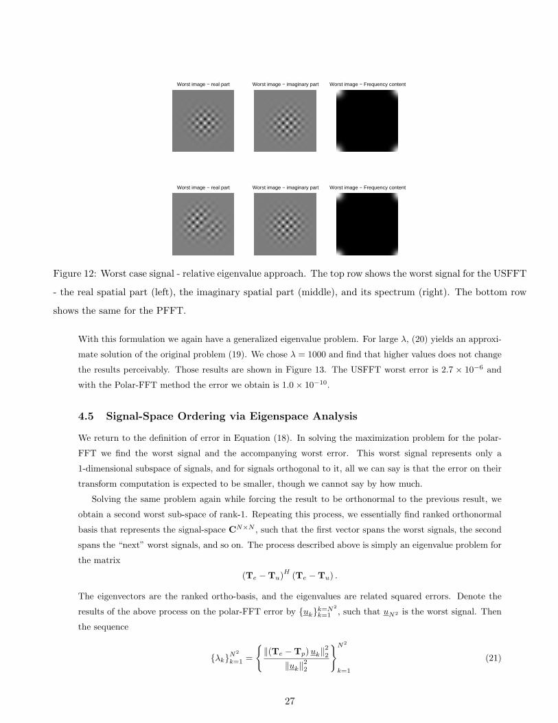
problem amounts to a generalized eigenvalue problem [34]. Figure 12 presents the results for cartesian
USFFT method (maximal error is 5.5 × 10⁻⁵) and Polar-FFT method (worst error is 6 × 10⁻⁸). Both
methods lead to similar worst-case signals, with energy mostly falling outside the circle of radius π, so that
the denominator in the above definition is nearly zero. Nevertheless, our Polar-FFT has advantages over
cartesian coordinates.
4.4.3 Relative Approach with Support Constraint
Finally, we seek the worst case signal for (18) with the side-constraint of no energy in the frequency domain
outside the circle of radius π. Thus we solve
maxx
‖(Te −Tu) x‖22‖Tex‖22
subject to F1x = 0, (19)
where F1 represents the regular cartesian FFT in a predetermined density, restricted to frequency points
outside the circle. Alternatively, we reformulate this using
max{x| F1x=0}
‖(Te −Tu)x‖22‖Tex‖22
≈ maxx
‖(Te −Tu)x‖22‖Tex‖22 + λ ‖F1x‖22
. (20)
26
Worst image − real part Worst image − imaginary part Worst image − Frequency content
Worst image − real part Worst image − imaginary part Worst image − Frequency content
Figure 12: Worst case signal - relative eigenvalue approach. The top row shows the worst signal for the USFFT
- the real spatial part (left), the imaginary spatial part (middle), and its spectrum (right). The bottom row
shows the same for the PFFT.
With this formulation we again have a generalized eigenvalue problem. For large λ, (20) yields an approxi-
mate solution of the original problem (19). We chose λ = 1000 and find that higher values does not change
the results perceivably. Those results are shown in Figure 13. The USFFT worst error is 2.7 × 10⁻⁶ and
with the Polar-FFT method the error we obtain is 1.0× 10⁻¹⁰.
4.5 Signal-Space Ordering via Eigenspace Analysis
We return to the definition of error in Equation (18). In solving the maximization problem for the polar-
FFT we find the worst signal and the accompanying worst error. This worst signal represents only a
1-dimensional subspace of signals, and for signals orthogonal to it, all we can say is that the error on their
transform computation is expected to be smaller, though we cannot say by how much.
Solving the same problem again while forcing the result to be orthonormal to the previous result, we
obtain a second worst sub-space of rank-1. Repeating this process, we essentially find ranked orthonormal
basis that represents the signal-space CN×N , such that the first vector spans the worst signals, the second
spans the “next” worst signals, and so on. The process described above is simply an eigenvalue problem for
the matrix
(Te −Tu)H (Te −Tu) .
The eigenvectors are the ranked ortho-basis, and the eigenvalues are related squared errors. Denote the
results of the above process on the polar-FFT error by {uk}k=N2
k=1 , such that uN2 is the worst signal. Then
the sequence
{λk}N2
k=1 =
{‖(Te −Tp)uk‖22
‖uk‖22
}N2
k=1
(21)
27

Worst image − real part Worst image − imaginary part Worst image − Frequency content
Worst image − real part Worst image − imaginary part Worst image − Frequency content
Figure 13: Worst case signal - relative eigenvalue approach with constraint. The top row shows the worst
signal for the USFFT - the real spatial part (left), the imaginary spatial part (middle), and its spectrum
(right). The bottom row shows the same for the PFFT.
measures the errors induced by each subspace, from ranked best to the worst. Using the same ortho-basis,
we may compute
{δk}N2
k=1 =
{‖(Te −Tu) uk‖22
‖uk‖22
}N2
k=1
, (22)
the errors we will effectively obtain from the cartesian USFFT method on the same subspaces. Plotting
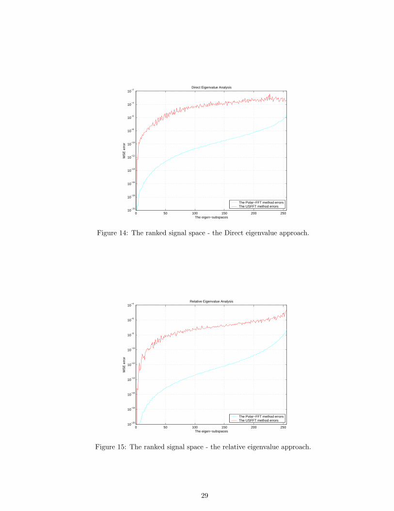
these two sequences in Figure 14, we compare the distribution of errors by subspace and obtain a complete
picture about the transform errors of the two methods for all the signal space.
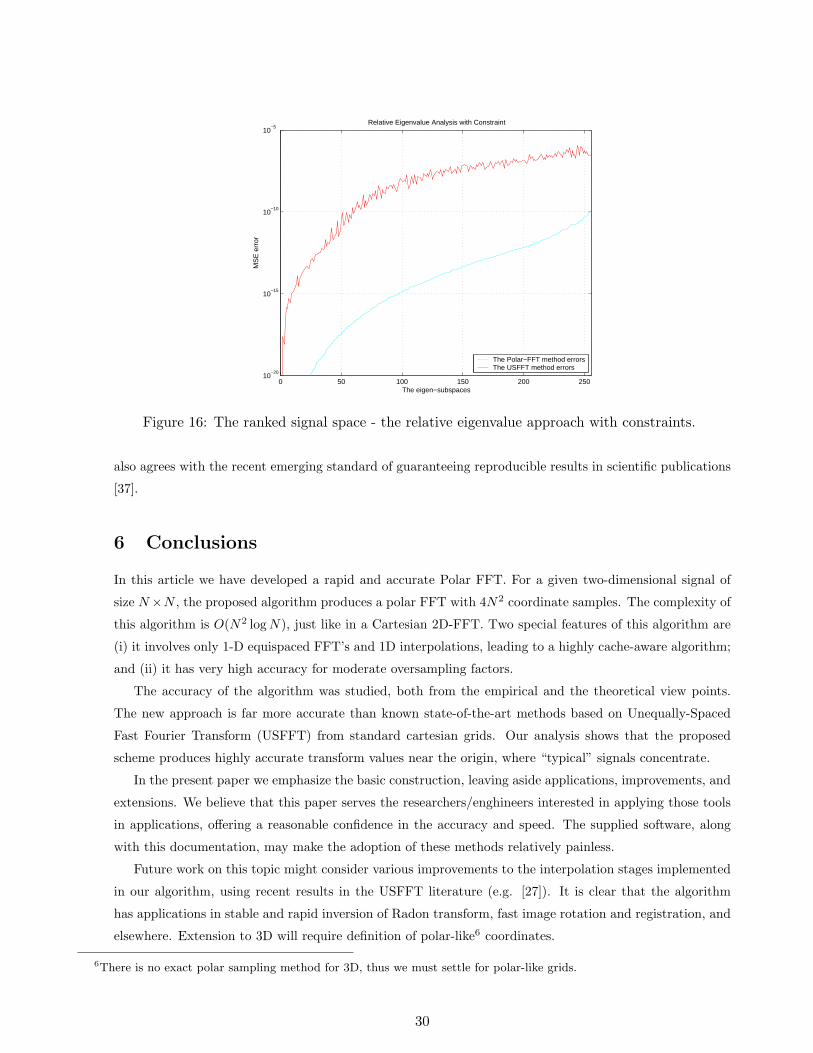
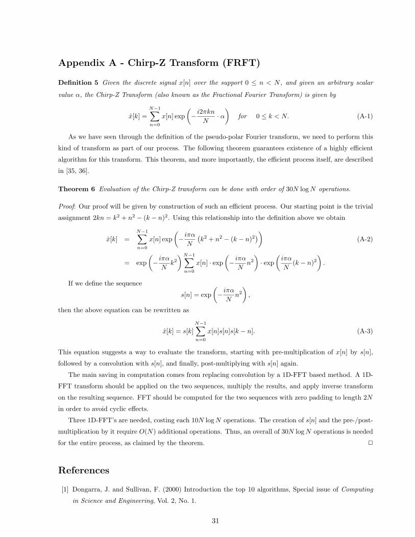
Figure 15 is similar but uses (19) to obtain the ortho-basis and the errors for its subspaces. In this case
the eigenvalue problem becomes a generalized eigenvalue one. Similarly, Figure 16 presents results from
the constrained generalized eigenvalue problem (20). All these figures show a consistent superiority of the
cartesian Polar-FFT over the USFFT method.
5 Available Software and Reproducible Results
One of the main objectives of this project has been development of a software tool that performs the compu-
tations given here. We intend to make this toolbox available to the public, in a fashion parallel to Wavelab
and Beamlab libraries [37, 38]. Our implementation uses Matlab code to perform various tasks around the
idea of polar FFT. The PFFT toolbox is freely available in http://www.stanford.edu/~elad/PolarFFT.zip.
As part of the freely available software, we supply code reproducing every figure based on computation
(as opposed to figures containing drawings). We believe that this will help researchers entering this area, and
engineers interested in better understanding the details behind the verbal descriptions supplied here. This
28
0 50 100 150 200 25010
−20
10−18
10−16
10−14
10−12
10−10
10−8
10−6
10−4
10−2
The eigen−subspaces
MS
E e
rror
Direct Eigenvalue Analysis
The Polar−FFT method errorsThe USFFT method errors
Figure 14: The ranked signal space - the Direct eigenvalue approach.
0 50 100 150 200 25010
−20
10−18
10−16
10−14
10−12
10−10
10−8
10−6
10−4
The eigen−subspaces
MS
E e
rror
Relative Eigenvalue Analysis
The Polar−FFT method errorsThe USFFT method errors
Figure 15: The ranked signal space - the relative eigenvalue approach.
29
0 50 100 150 200 25010
−20
10−15
10−10
10−5
The eigen−subspaces
MS
E e
rror
Relative Eigenvalue Analysis with Constraint
The Polar−FFT method errorsThe USFFT method errors
Figure 16: The ranked signal space - the relative eigenvalue approach with constraints.
also agrees with the recent emerging standard of guaranteeing reproducible results in scientific publications
[37].
6 Conclusions
In this article we have developed a rapid and accurate Polar FFT. For a given two-dimensional signal of
size N×N , the proposed algorithm produces a polar FFT with 4N2 coordinate samples. The complexity of
this algorithm is O(N2 log N), just like in a Cartesian 2D-FFT. Two special features of this algorithm are
(i) it involves only 1-D equispaced FFT’s and 1D interpolations, leading to a highly cache-aware algorithm;
and (ii) it has very high accuracy for moderate oversampling factors.
The accuracy of the algorithm was studied, both from the empirical and the theoretical view points.
The new approach is far more accurate than known state-of-the-art methods based on Unequally-Spaced
Fast Fourier Transform (USFFT) from standard cartesian grids. Our analysis shows that the proposed
scheme produces highly accurate transform values near the origin, where “typical” signals concentrate.
In the present paper we emphasize the basic construction, leaving aside applications, improvements, and
extensions. We believe that this paper serves the researchers/enghineers interested in applying those tools
in applications, offering a reasonable confidence in the accuracy and speed. The supplied software, along
with this documentation, may make the adoption of these methods relatively painless.
Future work on this topic might consider various improvements to the interpolation stages implemented
in our algorithm, using recent results in the USFFT literature (e.g. [27]). It is clear that the algorithm
has applications in stable and rapid inversion of Radon transform, fast image rotation and registration, and
elsewhere. Extension to 3D will require definition of polar-like6 coordinates.
6There is no exact polar sampling method for 3D, thus we must settle for polar-like grids.
30
Appendix A - Chirp-Z Transform (FRFT)
Definition 5 Given the discrete signal x[n] over the support 0 ≤ n < N , and given an arbitrary scalar
value α, the Chirp-Z Transform (also known as the Fractional Fourier Transform) is given by
x[k] =N−1∑n=0
x[n] exp(− i2πkn
N· α
)for 0 ≤ k < N. (A-1)
As we have seen through the definition of the pseudo-polar Fourier transform, we need to perform this
kind of transform as part of our process. The following theorem guarantees existence of a highly efficient
algorithm for this transform. This theorem, and more importantly, the efficient process itself, are described
in [35, 36].
Theorem 6 Evaluation of the Chirp-Z transform can be done with order of 30N log N operations.
Proof: Our proof will be given by construction of such an efficient process. Our starting point is the trivial
assignment 2kn = k2 + n2 − (k − n)2. Using this relationship into the definition above we obtain
x[k] =N−1∑n=0
x[n] exp(− iπα
N
(k2 + n2 − (k − n)2
))(A-2)
= exp(− iπα
Nk2
) N−1∑n=0
x[n] · exp(− iπα
Nn2
)· exp
(iπα
N(k − n)2
).
If we define the sequence
s[n] = exp(− iπα
Nn2
),
then the above equation can be rewritten as
x[k] = s[k]N−1∑n=0
x[n]s[n]s[k − n]. (A-3)
This equation suggests a way to evaluate the transform, starting with pre-multiplication of x[n] by s[n],
followed by a convolution with s[n], and finally, post-multiplying with s[n] again.
The main saving in computation comes from replacing convolution by a 1D-FFT based method. A 1D-
FFT transform should be applied on the two sequences, multiply the results, and apply inverse transform
on the resulting sequence. FFT should be computed for the two sequences with zero padding to length 2N
in order to avoid cyclic effects.
Three 1D-FFT’s are needed, costing each 10N log N operations. The creation of s[n] and the pre-/post-
multiplication by it require O(N) additional operations. Thus, an overall of 30N log N operations is needed
for the entire process, as claimed by the theorem. 2
References
[1] Dongarra, J. and Sullivan, F. (2000) Introduction the top 10 algorithms, Special issue of Computing
in Science and Engineering, Vol. 2, No. 1.
31

[2] Natterer, F. (1986) The Mathematics of Computerized Tomography. John Wiley & Sons, New York.
[3] Briggs, B. and Henson, E. (1995) The FFT: an Owner’s Manual for the Discrete Fourier Transform,
SIAM, Philadelphia.
[4] Unser, M., Thevenaz, P. and Yaroslavsky, L. (1995), IEEE Trans. on Image Processing, Vol. 4, No. 10,
pp. 1371–1381.
[5] Keller, Y., Averbuch, A., and Israeli, M. (2003) A PseudoPolar FFT technique for translation, rotation
and scale-invariant image registration, Accepted to the IEEE Trans. On Image Processing.
[6] Irani, M., Rousso, B. and Peleg, S. (1997) Recovery of ego-motion using region alignment IEEE Trans.
on Pattern Analysis and Machine Intelligence, Vol. 19, No. 3, pp. 268–272.
[7] Basu, S. and Bresler, Y. (2000) An O(n2 log n) filtered backprojection reconstruction algorithm for
tomography, IEEE Trans. Image Processing, Vol. 9, No. 10, pp. 1760–1773.
[8] Parker, J.A., Kenyon, R.V. and Troxel, D.E. (1983) Comparison of interpolating methods for image
resampling, IEEE Trans. on Medical Imaging, Vol. 2, pp. 31-39.
[9] Stark, H., Woods, J.W., Paul, I. and Hingorani, R. (1981) Direct Fourier reconstruction in computer
tomography, IEEE Trans. on Acoustics, Speech and Signal Proc. Vol. 29, No. 2, pp. 237-245.
[10] Fan, H. and Sanz, J.L.C. (1985) Comments on ’Direct fourier reconstruction in computer tomography’,
IEEE Trans. on Acoustics, Speech and Signal Proc., Vol 33, No. 2, pp. 446-449.
[11] Matej, S. and Vajtersic, M. (1990) Parallel implementation of the direct Fourier reconstruction method
in tomography, Computers and Art. Intel., Vol. 9, No. 4, pp. 379–393.
[12] Moraski, K. J. and Munson Jr., D.C. (1991) Fast tomographic reconstruction using chirp-z interpola-
tion, in Proceedings of 25th Asilomar Conference on Signals, Systems, and Computers, Pacific Grove,
CA, pp. 1052-1056.
[13] Choi, H. and Munson Jr., D.C., (1998) Direct-Fourier reconstruction in tomography and synthetic
aperture radar, Int. J. of Imaging Systems and Tech., Vol.9, No.1, pp. 1-13.
[14] Walden, J. (2000) Analysis of the direct Fourier method for computer tomography, IEEE Trans. on
Medical Imaging, Vol. 19, No.3, pp. 211–22.
[15] Gottleib, D., Gustafsson, B., and Forssen, P. (2000) On the direct Fourier method for computer
tomography, IEEE Transactions on Medical Imaging, Vol. 19, No. 3, pp. 223–232.
[16] Suli, E. and Ware, A. (1991) A spectral method of characteristics for hyperbolic problems SIAM J.
Numer. Anal., Vol. 28, No. 2, pp. 423–445.
[17] Boyd, J.P. (1992) Multipole expansions and pseudospectral cardinal functions: A new generalization
of the Fast Fourier Transform, J. Comput. Phys., Vol. 103 No. 2, pp. 184–186.
[18] Boyd, J.P. (1992) A fast algorithm for Chebyshev, Fourier, and sinc interpolation onto an irregular
grid, J. of Comp. Phys., Vol. 103, No. 2, pp.243–257.
[19] Beylkin, G. (1995) On the fast Fourier transform of functions with singularities, Applied Computational
Harmonics, Vol. 2, pp. 263-381.
32
[20] Anderson, C. and Dahleh, M. D. (1998) Rapid computation of the discrete Fourier transform, SIAM
J. Sci. Comput., Vol. 17 pp. 913–919.
[21] Dutt, A. and Rokhlin, V. (1993) Fast Fourier transforms for nonequispaced data, SIAM J. Sci. Com-
put., Vol. 14, pp. 1368–1393.
[22] Dutt, A. and Rokhlin, V. (1995) Fast Fourier transforms for nonequispaced data II, Appl. Comput.
Harmon. Anal. Vol. 2, pp. 85–100.
[23] Ware, A. F. (1998) Fast approximate Fourier transform for irregularly spaced data, SIAM Review, Vol.
40, No. 4, pp. 838–856.
[24] Potts, D., Steidl, G. and Tasche, M. (2000) Fast Fourier transforms for nonequispaced data: A tutorial,
in Modern Sampling Theory: Mathematics and Application by J. J. Benedetto and P. Ferreira, eds.,
ch. 12, pp. 253 - 274, Birkhauser.
[25] Duijndam, A.j.W. and Schonewille, M.A. (1999), Nonuniform fast Fourier transform, Geophysics, Vol.
64, No. 2, pp. 539–551.
[26] Nguyen, N. and Liu, Q.H. (1999) The regular Fourier matrices and nonuniform fast Fourier Transforms,
SIAM Journal of Scientific Computing, Vol. 21, No. 1, pp. 283–293.
[27] Fessler, J.A., and Sutton, B.P. (2003) Nonuniform Fast Fourier Transforms Using Min-Max Interpola-
tion, IEEE Trans. on Signal Processing, Vol. 51, No. 2, pp. 560–574.
[28] Averbuch, A., Coifman, R., Donoho, D.L., and Israeli, M. (2003) Fast Slant Stack: A notion of Radon
transform for data in a Cartesian grid which is rapidly computible, algebraically exact, geometrically
faithful and invertible, to appear in SIAM Scientific Computing.
[29] Porat, B. (1997) A Course in Digital Signal Processing, John Wiley & Sons.
[30] Mersereau, R. M. and Oppenheim, A. V., (1974) Digital reconstruction of multidimensional signals
from their projections, Proc. IEEE, Vol. 62, No. 10, pp. 1319–1338.
[31] Pasciak, J.E. (1981) A note on the Fourier algorithm for image reconstruction, Preprint AMD 896
Applied Mathematics Department, Brookhaven National Laboratory, Upton, New York 11973.
[32] Edholm, P. and Herman, G.T., (1987) Linograms in image reconstruction from projections ,IEEE
Trans. Medical Imaging, MI-6, No. 4, pp. 301-307.
[33] Lawton, W., (1988) A new polar fourier-transform for computer-aided tomography and spotlight syn-
thetic aperture radar Ieee Transactions On Acoustics Speech And Signal Processing, Vol. 36, No. 6, pp.
931–933 June 1988.
[34] Golub, G.H. and Van Loan C.F, (1996) Matrix Computations, John Hopkins University Press, Third
edition.
[35] Rabiner, L. R., Schafer, R. W. and Rader, C. M. (1969) The Chirp z-Transform algorithm and its
application”, Bell System Technical Journal, Vol. 48 pp. 1249–1292.
[36] Bailey, D. H. and Swarztrauber P. N. (1991) The fractional Fourier transform and applications, SIAM
Review, Vol. 33, No. 3 pp. 389–404.
33

[37] Buckheit, J. and Donoho, D.L. (1995) WaveLab and Reproducible Research, in Wavelets and Statistics,
Springer-Verlag, Berlin.
[38] Choi, C.S., Donoho, D.L., Flesia, A.G., Huo, X., Levi, O., and Shi, D. (2002) About BeamLab a
Toolbox for New Multiscale Methodologies, Stanford University - Statistics Department Technical
Report, http://www-stat.stanford.edu/~beamlab.
34