farm optimization for households growing oilseed …
TRANSCRIPT
FARM OPTIMIZATION FOR
HOUSEHOLDS GROWING OILSEED
CROPS IN JIMMA, ETHIOPIA.
Napol D. Gurmesa
Supervisors:
Ir. Jo Wijnands
Agricultural Economics
Research Institute
LEI, The Hague
Ir. Gerard Giesen Business Economics Group
Wageningen University
Thesis Business Economics: BEC 80433
Wageningen
May 2011

2
Abstract:
The main objective of this MSc thesis was to develop a farm optimization model for
households that grow oilseeds and other crops in Jimma region. Developing a farm
model was necessary to address due to lacking economic farm research on this
subject in Ethiopia. In doing so, 11 crops (teff, wheat, sorghum, maize, faba beans, field
peas, soya bean, nueg, linseed, sunflower and sesame) were included in the model.
Along with the crops, the major agronomic (rainfall, land and soil) and socio-economic
conditions (labor, food security and financial capital) that affect the farm practice
were taken into account. As a goal, the gross farm income from these crops was
maximized by the model.
The optimization results were separately assessed for the conventional and best farm
practices. Under both farm practices, the cropping plan was more or less the same.
Maize had the highest share of land (mostly 50%) under most cropping plan of
different farm sizes. Apart from the cereals, that consumed the maximum allowed land
in all cases (67%), sesame and to a lesser extent soya beans together utilized most of
the land left (mostly more than 25%). Small farm size has proven to have a negative
impact on the gross farm incomes due to the prevalence of a minimum acreage land
required to meet their food demand.
Land was the most common binding resource. A significant difference between the
optimal results of conventional and best farm practices was recognized when the
effect of constraints was assessed through sensitivity analysis. Under best farm
practices, limiting credit facilities has proven to have a far more negative impact,
which resulted in fallow lands and extremely low discretionary incomes. The
participation of oilseed crops in the optimal plans was mainly represented by sesame
and soya beans. Price rises in soya bean improve the land share of soya bean, but not
that of sunflower, nueg and linseed. The model led to a number of new, interesting
and relevant research topics. It can also be made more comprehensive by including
other factors, which can be a stepping stone for future Ethiopian researches in the
area.
Key words: farm optimization, agronomic constraints, socio-economic constraints,
gross farm income, conventional farming, best farm practices, cropping plan, cereals,
oilseed crops.

3
Preface
The accomplishment of this MSc thesis would not be possible without the valuable
contribution of a number of people that have supported me during all these years. I
feel that the least I can do is acknowledge and thank them.
My dear supervisors, Ir. Jo Wijnands and Ir. Gerard Giesen, were basically the bed
rocks of my thesis. Jo instructed me from day 1 and relentlessly gave me critical
methodological and academic insights. Every time we met, I learned something from
him and I felt my growth intellectually and professionally throughout the process.
Gerard, on the other hand, has been a great controller and care taker of my thesis.
Without his support and supervision, my thesis would not meet the necessary
thresholds. His rich experience with economic principles and modeling has been
instrumental in providing me with critical directions and recommendations on how I
should proceed every step of the way.
I would also like to thank Ir. Robert van Loo from Plant Science Group. He has been
impressively responsive whenever I wanted his help. Biological and agronomic issues
were beyond my scope of knowledge and Robert contributed a great insight in filling
the gap. He also taught me how to use GAMS, which was invaluable.
And thanks to my colleague and roommate, Jolinda Lute, who has accompanied me
during the academic trips and coffee breaks. Our spontaneous chats and jokes have
kept my work interesting and stimulating. Finally, I would like to thank my family
(dad, mom and sis), who showed me all the love throughout my life and who are
actually the reason why I live.
4
Table of Contents 1 Introduction ........................................................................................................... 7
1.1 Background of the study ...................................................................................... 7
1.2 Research problem ................................................................................................. 8
1.3 Objective of the study ........................................................................................... 9
1.4 Methodology .......................................................................................................... 9
1.4.1 Brief description of the study area ...................................................................... 9
1.4.2 Data type and data Source .................................................................................. 10
1.4.3 Data collection method ....................................................................................... 10
1.5 Methods of data analysis .................................................................................... 11
1.6 Scope of the study ............................................................................................... 11
1.7 Outline of the thesis ............................................................................................ 11
2 Literature on farm optimization models............................................................... 12
2.1 Farm optimization .............................................................................................. 12
2.2 Farm household model objectives ..................................................................... 14
3 Farming in Ethiopia ................................................................................................ 16
3.1 General information on farming in Ethiopia .................................................... 16
3.2 The Ethiopian government agricultural policy ................................................ 17
3.3 Inputs of peasant farming in Ethiopia ............................................................... 18
3.4 Agronomic conditions ........................................................................................ 18
3.4.1 Rainfall ................................................................................................................. 18
3.4.2 Land and soil ....................................................................................................... 19
3.5 Socio-economic conditions ................................................................................ 20
3.5.1 Labor .................................................................................................................... 20
3.5.2 Food security ....................................................................................................... 20
3.5.3 Credit .................................................................................................................... 21
4 Model description and data interpretation .......................................................... 23
4.1 General structure ................................................................................................ 23
4.2 Explanation of the general structure ................................................................. 25
4.3 The objective function ........................................................................................ 26
4.4 The Crops ............................................................................................................. 27
4.5 Constraints- conventional farm practice .......................................................... 29
4.5.1 Land constraint ................................................................................................... 29
4.5.2 Rotational constraints ........................................................................................ 29
4.5.3 Labor requirement .............................................................................................. 31
4.5.3.1 General Activities ............................................................................................ 32
4.5.3.2 Soil Tillage ....................................................................................................... 33
4.5.3.3 Sowing – weeding ........................................................................................... 34
4.5.3.4 Harvesting, threshing and cleaning ............................................................... 35
4.5.4 Fertilizer and sowing seed requirement and costs .......................................... 35
4.5.5 Food requirement ............................................................................................... 36
4.5.6 Crop yield balance .............................................................................................. 38
4.5.7 Cash flow requirement ....................................................................................... 38
4.6 Best farm practices ............................................................................................. 39

5
4.7 Summary information of crops .......................................................................... 41
5 Results of the model ............................................................................................... 43
5.1 Validation of the model ...................................................................................... 43
5.2 Conventional practice results ............................................................................ 46
5.2.1 Optimum plan results ......................................................................................... 46
5.2.2 Sensitivity analysis.............................................................................................. 50
5.2.2.1 Increase in price of soya bean and sunflower .............................................. 50
5.2.2.2 Low labor supply ............................................................................................. 52
5.3 Best farm practice results .................................................................................. 54
5.3.1 Optimum plan results ......................................................................................... 54
5.3.2 Sensitivity analysis.............................................................................................. 56
5.3.2.1 Increasing price of soya bean and sunflower ............................................... 56
5.3.2.2 Credit ................................................................................................................ 58
5.3.2.3 Low labor supply ............................................................................................. 59
6 Discussions, conclusions and recommendations ................................................. 61
6.1 Methodological issues......................................................................................... 61
6.1.1 Model re-usability and representation ............................................................. 61
6.1.2 Crop rotation scheme ......................................................................................... 61
6.1.3 Assumptions made in the thesis ........................................................................ 63
6.2 General discussion of results ............................................................................. 64
6.3 Conclusions from results .................................................................................... 66
6.4 Recommendations for future researches.......................................................... 67
References (Literature and websites) ........................................................................... 68
Appendix 1:Man labor hours ......................................................................................... 72
Appendix 2: Oxen labor hours ....................................................................................... 79
Appendix 3: Production and utilization ........................................................................ 83
Appendix 4: Fertilizer and seed input ........................................................................... 83
Appendix 5: Crop rotation table .................................................................................... 84
Appendix 6: Costs (Inputs, hiring and food) in ETB..................................................... 85

6
List of Tables:
Table 1 Share of Agriculture in Ethiopian GDP ................................................................ 16
Table 2 Consumption in 2007 and dietary reference intake of energy, proteins and fats .............................................................................................................................................. 21
Table 3 General Structure of the LP model ....................................................................... 24
Table 4 Area and yield in kg/ha of the main crops in Jimma and Ethiopia (Italic are selected crops) .................................................................................................................... 28
Table 5 Distribution of Agricultural households by holding size in hectares ................ 29
Table 6 Soil tillage ............................................................................................................... 34
Table 7 Farm gate and Seed Price of the crops ................................................................. 36
Table 8 Food consumption computation .......................................................................... 37
Table 9 Major differences between the two farm practices. ........................................... 40
Table 10 Crop summary under conventional farm practices ......................................... 41
Table 11 Crop summary under best farm practices ........................................................ 42
Table 12 Actual and optimal cropping plan results at the average farm size of 1.72 hectares ................................................................................................................................ 44
Table 13 Optimal cropping plan and economic results for conventional farm practices at different farm sizes ......................................................................................................... 47
Table 14 Price* increase impacts of soya bean and sunflowers at the 5 hectare
conventional farm ............................................................................................................... 51
Table 15 Impact of low labor supply and higher labor price at conventional farm size of 5 hectares ........................................................................................................................ 52
Table 16 Optimal crop plan results for best farm practices at different farm sizes ...... 54
Table 17 Increasing price of soya bean (4.0) and sunflower (5.25) at a farm size of 5 hectares. ............................................................................................................................... 57
Table 18 Changes in credit level at a (best practice) farm size of 5 hectares ............... 58
Table 19 Impact of low labor supply at farm size of 5 hectares ..................................... 59
Table 20 Results of other rotation rules at farm size of 5 hectares ............................... 62
List of Figures Figure 1 Location of the Study………………………………………………………….............................10
Figure 2 Structure of the farm household……………………………………………….. ...................14
Figure 3 Annual rain variability…………………………………………………………...........................19
Figure 4 Crop Calendar of Ethiopia……………………………………………………............................30
Figure 5: Percentage utilized of production in 2008/2009 (2001 E.C.)..............................37

7
1 Introduction
In this chapter, background information on crop agriculture in Ethiopia will be first
presented. Then, the research problem, the research objectives and questions will be
outlined. Finally, the general methodology used in the thesis will be explained
followed by the scope and organization of the thesis.
1.1 Background of the study
Agriculture is the most important sector of the Ethiopian economy in terms of income,
employment and Gross Domestic Product (GDP). According to Fitsum et al. (2006),
agriculture’s contribution to GDP, although showing slight decline over the years, has
remained very high. Currently, agriculture employs 80% of the national labour force
and accounts for 47% of the GDP (Wijnands et al., 2009).
Crop production, among all agricultural activities, is the major contributor to the GDP.
The peasant sector, which produces more than 90 per cent of crop output has simple
farming technology, acute shortage of purchased inputs particularly fertilizer, little
infrastructure and inefficient marketing systems (Arbrar, 2003). With 85 percent of
the population (75 million) living in rural areas under subsistence and semi-
subsistence (CSA, 2000), Ethiopia needs to accelerate agricultural growth
(Gabre_Madhin and Goggin, 2005; Gabre Madhin, 2001).
The oilseeds sector, which is a subset of crop production, is Ethiopia’s fastest-growing
agricultural sector, both in terms of its foreign exchange earnings and as a main
source of income for over three million Ethiopian farmers. It is the second largest
source of foreign exchange earnings after coffee. Study reports indicate that Ethiopia
is among the top-five producers of sesame seed, linseed and noug, also called neug or
niger seed (Wijnands et al, 2009).
Despite its rising significance, stakeholders are convinced that the oilseed production
in Ethiopia hasn’t reached its climax. Gelalcha (2009) and Wijnands et al. (2009)
asserted that the potential for further growth, both in terms of quantity and quality of
oilseed crops, through improved production techniques and productivity factors is
considered to be great. In addition, evidences point to a growing export of oilseed
from Ethiopia to the rest of the world in general.
Many oilseed crops remain largely unknown to a large proportion of Ethiopian
farmers. In the region of Jimma for instance, oilseed crops such as soya beans,
sunflower and sesame are being introduced as new crops on an established farm.
Noug and linseed are the only two major oilseed crops prominently grown in the
region (CSA, 2009). Cereals and pulses are by far more known and grown. Cereals in
particular are grown over a significant chunk of Ethiopian farms, signalling a large
room for oilseed crops to expand their land share.

8
In the process of introducing the oilseed crops on the farms of Jimma, the primary
farm inputs, land, labor and capital are shared with other crops, mainly cereals and
pulses. This means competition among the traditional and new crops. The higher
resource competition and the introduction of new crops sparks a need for a
comprehensive farm model, which facilitates an understanding of the new farm
dynamics.
The new farm dynamics set up a different agronomic and socio-economic
environment. This is due to the fact that any crop grown over a farm has to qualify
both agronomic (soil fertility, rainfall, altitude, crop rotation) and socio-economic
possibilities (land availability, labor, food security). Hence, there is considerable need
for a model that involves the new crops to address the new farm dynamics and that
handles the stronger resource competition between the crops.
As far as we know, there is no farm optimization research at household level for
Ethiopian cases that incorporates these crops. The household models that have been
developed so far (Singh, 1987) couldn’t give a complete focus on crop production. This
study will address this research gap by developing a linear programming farm model
that maximizes income from these crops. Linear programming is still one of the most
widely used optimization model techniques used in modern business. According to
Claassen et al (2007), ever since linear programming was introduced, it has been in
wide use.
1.2 Research problem
Although oilseeds are widely regarded as a great business engine for the Ethiopian
economy, there are no or limited integrated studies of oilseed crop production at farm
level along with cereals and pulses.
The Ethiopian Institute of Agricultural Research (EIAR), which is the major farm
research institute in the country, gives little attention to researches on economic farm
modeling. The core mandates of EIAR are; supply of improved agricultural
technologies, popularization of improved technologies and coordination of the
national agricultural researches (EIAR, 2010). Hence, it is safe to conclude that much
of the focus goes to technological issues. Tesfaye (2007) outlined the socio-economic
research branch of EIAR as only focusing on methods of participatory research and
technology transfer, monitoring and evaluation of technology packages with regard to
adoption and impact, and contributions to policies. Thus, there is a clear gap of
knowledge with regard to farm modeling.
The knowledge gap has prevented policy makers, business managers and other stake
holders from making well informed decisions in the past. This bottleneck also had its
role in depressing the attempts to improve overall crop yields and gross farm incomes.
Having adequate well-presented information will improve the efficiency of rural
development projects and programs (Samuel, 2006a). This research addresses the

9
knowledge gap by developing a linear optimization model for the crops could help
planners as well as future researchers.
1.3 Objective of the study
The main objectives of this study are:
1. To develop a farm optimization model that involves both oilseed and other
crops grown in Jimma region.
2. To analyze the new farm dynamics created by introducing oilseed crops on an
average Jimma farm and assess the effect of different factors on cropping plan
and income of the farmers.
The objectives of the thesis are reflected in an attempt of answering the following
research questions:
a) What are the key crops, including oilseeds, that can be grown in Jimma region?
b) Do these crops fit the actual farm practice?
c) What are the prominent agronomic and socio-economic restrictions in
maximizing the income from these crops?
d) How can these crops and restrictions be modelled in line with the analysis of
the major crop information such as labour requirement, expenses, returns, etc?
e) What are the optimum results of the model?
f) How do the various restrictions and variables affect the optimum results and
what is the effect of different scenarios?
1.4 Methodology
Chapter 3 reviews the overall methodology in developing the optimization model. In
this section, a brief description of the study area is presented followed by the data
sources for the model and the method of analysis used to extract results of the model.
1.4.1 Brief description of the study area
This study is about the region of Jimma (see figure 1.1). Jimma is one of the 13 zones
in Oromiya region in the southwestern part of Ethiopia. It has about 2.5 million people
of which 5.7% are urban dwellers and 94.3% are rural dwellers (CSA, 2007). Jimma is
known for its rich coffee. Most of Jimma’s landscape is midlands which constitute 67%
of the land.

10
Figure 1 Location of the Study
Source: Jimma University, 2006
1.4.2 Data type and data Source
This research mainly relies on secondary data sources of both quantitative and
qualitative nature. The secondary data sources include CSA (Central Statistical Agency
of Ethiopia) data, government reports, scientific papers and literature reviews.
The CSA database is used to identify the key crops and oilseeds that are
predominantly cultivated in Jimma region. This assists the choice of crops to be
included in the model. CSA data also provides the general information such as average
yields, rough fertilizer consumption estimates, and other resource requirements.
Moreover, literatures depicting the general agronomic and socio economic nature of
Ethiopian agriculture are extensively used to identify the major agricultural
restrictions. In addition, government reports, Agricultural Association reports are also
part of the assessment to cross check facts and solidify findings.
1.4.3 Data collection method
The research is conducted in the Netherlands. So, there is no field assessment and face
to face interviews with farmers. Since secondary data is mainly used, much of the data
collection is done by reviewing all the sources mentioned above. To fit the data
available to the purpose of this research, some restructuring of the available data is
carried out.

11
1.5 Methods of data analysis
In this study, collected data is analyzed using different quantitative and qualitative
statistical procedures and methods. Descriptive statistical measures such as means
and percentages are used to summarize raw data available about Jimma region. This
assists in producing input data or resource consumption data for the crops.
Further data interpretation is assisted by mathematical programming software
known as GAMS. Gross farm income data and constraints data will be fed in to the
software to perform actual optimization and sensitivity analysis. Hence, the nature of
the analysis is mainly quantitative. However, qualitative data will be partly analyzed
on spot during data collection to fill the gaps in the quantitative data.
1.6 Scope of the study
This study is a part of an oilseed project in Ethiopia, which is undertaken by the
cooperation between LEI and PRI of Wageningen University and Research Centre. The
farm model, which is a central theme of this thesis, is specifically developed for the
region of Jimma, situated in the Southwest corner of Ethiopia. But the model can serve
as a basic framework of analysis for areas with similar social, agronomic and
topographic conditions. The main objective of the model is income maximization of
farmers. Hence, other possible model objectives such as cost minimization, efficiency
promotion and resource optimization are not emphasized as a priority. In addition to
this, the model is developed on the themes of linear programming and reflects the
possibility of growing 11 crops indicated on a certain farm in the region.
In terms of the variables and constraints taken in to consideration, only a number of
socio-economic and agronomic restrictions that have a limiting influence on gross
farm income were incorporated. These constraints include land, labor, food security,
fertilizer, cash flow and credit limitations. In this regard, the most important
constraints critical to the farm conditions of the region were taken in to account.
Lastly, the findings from this research can be applied to some areas other than Jimma.
1.7 Outline of the thesis
Chapter 1 is the introduction chapter. Research problems, objectives and
methodology followed in carrying out the research are presented. In chapter 2, a brief
review of literature on farm optimization models is presented. Chapter 3 provides the
basic information on Ethiopian farming. Chapter 4 describes the structure of the farm
model and specifies the method used in developing the major parts of the model. This
chapter narrows down the general background information discussed about
Ethiopian farming in chapter 3 to the region of Jimma and specifies how the model is
built for the region along the way. In chapter 5, the main results from the model
calculations are presented and explained. Finally, chapter 6 presents the discussions
and conclusions of this study.

12
2 Literature on farm optimization models
In this chapter, two major areas of knowledge pertaining to this research will be
briefly addressed. First, the concepts pertinent to farm optimization in general will be
briefly discussed. Then a pointed discussion relating the household and farm will be
made.
2.1 Farm optimization
Developing farm optimization models is related with planning more than any other
conventional management functions. The function of planning in business is covered
in various literature and books advocating it as a very critical activity for ensuring
business success. The function of planning as a decision making unit in business is
well known. To match this notion in farming, Barnard and Nix, (1999) asserted that
the farmer is the manager or the entrepreneur of a farm who carries out decision
making activities including the function of planning. Planning in business sense is the
process of setting organization goals and determines the best strategy in reaching
them. In relation to farms, farm models assist how the resources should be allocated
enriching more understanding of farms.
Farmers often have little patience with economic principles and tend to dismiss
scientific ideas of management functions (Schweigman, 2005). It is true that there are
considerable variations and uncertainties between what literature say and what
farmers actually face making it difficult to provide neat answers to individual farm
situations. Nevertheless, knowledge of these principles is important for better
planning and decision making.
The decisions taken in farm planning are not fundamentally different from those that
need to be taken in manufacturing or service industry. Barnard and Nix, (1999)
pointed out three basic decisions in farm planning:
1. What to produce? That is which activities or a combination of activities an
enterprise chooses to carry out. Product-product relationships are usually studied
to answer this question.
2. How much to produce? That is at which level of output should be aimed in each
enterprise. It relates to factor-output relationship.
3. How to Produce? This answers which combination of resources (alternatively
factors or inputs) should be used to produce the products the enterprise selected.
The supply of some resources is limited, thus restricting the choice. Here, factor-
factor relationships are relevant.
Schweigman (2005) also went on describing the basics of farm planning in terms of
crop farming as a combined decision of what, when, how and how much is grown.
Most of these questions focused on crops while dealing with farming, which fits the
purpose of the thesis. Schweigman (2005) described these decisions in real farm
conditions as:

13
“What is grown depends, among other things, on the character of the soil,
availability of water, climate and tradition. When to grow appears in the so called
growing-calendar. This gives the points of time on which to start planting or
harvesting (growing season). The growing calendar is very much regionally defined.
How to grow crops is associated with how often one weeds, how much fertilizer is
used, how land is tilled with a hoe or with ox-drawn ploughs, etc. This is mainly where
the manual labor is consumed. Lastly, how much must be grown is described by what
size of acreage should be for every crop or combination of crops.”
These decisions and farm activities are usually reflected best in farm models. Romero
and Rehman (1984) depicted the structure of decision making in farm planning as a
linear programming model as:
Max.z = f (x ) = c ' x
subject to
A x<= b and
X >= 0
Where
z the criterion function (usually defined as profit before deducting fixed costs), is
a scalar product of _c' and x;.
x is a vector of decision variables. This might be the number of hectares a crop to
be grown, or the quantity of each crop to be produced, etc.
c ' is the vector giving corresponding contributions of these variables to the
criterion function.
b The vector b represents the physical, institutional and personal restraints that
define the environment within choices are made. This refers to the individual
economic contribution of each crop to the total economic benefit. It
specifies the limits of each restraint. This might be the maximum number of
crops in a certain crop rotation, the maximum labor hours available, the timing
that must be followed as a result of growing calendar, etc.
A defines the technical relationships between the variables and the constraints. In
other words, it refers to the requirement of a unit of each crop for each restraint.
This can be the number of labor hours per crop, the food consumed per each
crop, the amount of fertilizer to be utilized for each crop, etc.
Farm level planning usually involves financial objectives such as profit maximization.
Other objectives such as peer group standing (Gasson, 1973) and stable level of
income (Barnard and Nix, 1999) are also relevant. However, financial objectives are
commonly used in farm planning. (Glen ,1986). As indicated, the basic model of farm
planning is linear in its core essence. Linearity requires the following assumptions
(Bazaraa et al., 1990):
14
• Proportionality – a change in a variable results in a proportionate change in
that variable contribution to the value of the function;
• Additivity – the function value is the sum of the contributions of each term;
• Divisibility – the decision variables can be divided in to non-integer values,
taking fractional values. Integer programming techniques can be used if the
divisibility assumption does not hold;
• Deterministic – the coefficients are known and constant.
Despite these restrictive assumptions, linear programming models are among the
most widely used models today, representing several systems quite satisfactorily and
they can provide a large amount of information besides simply a solution
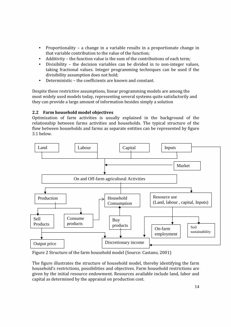
2.2 Farm household model objectives
Optimization of farm activities is usually explained in the background of the
relationship between farms activities and households. The typical structure of the
flow between households and farms as separate entities can be represented by figure
3.1 below.
Figure 2 Structure of the farm household model (Source: Castano, 2001)
The figure illustrates the structure of household model, thereby identifying the farm
household’s restrictions, possibilities and objectives. Farm household restrictions are
given by the initial resource endowment. Resources available include land, labor and
capital as determined by the appraisal on production cost.
Land Labour Inputs
On and Off-farm agricultural Activities
Production
Market scenario
Household Consumption
Discretionary income Output price
Resource use (Land, labour , capital, Inputs)
Consume products
Sell Products
On-farm employment
Soil sustainability
Buy products
Capital

15
Farm household possibilities are given by on and off-farm production activities. On
farm activities are defined for crop and fallow activities, while off-farm production
activities refer to off-farm employment possibilities for family laborers.
Production is either destined to the market or used for on-farm consumption. The
farm household can buy food and other products that are not produced at the farm.
Goods as well as factors can be bought on the market at market prices, while family
labor can also be hired out against the prevailing off-farm wage rate.
The household model pursues four objectives: maximum discretionary income,
minimum soil erosion, minimum risk and maximum on-farm employment.
Discretionary income is defined by Campell and McConnel, (1999) as the “amount of
farmer’s income available for spending after the essentials (such as production costs,
food, clothing, health and shelter) have been taken care of”. The result is a part of the
disposable income that can be used to finance vacations to retirement or invested or
saved fully at the farmer’s discretion. In this research, a term closely related to
discretionary income called as Gross Farm Income (GFI) is maximized.
There are some differences between gross farm income (the model objective of this
research) and discretionary income (as defined in Castano model). Firstly,
discretionary income is the residual result of deducting all production costs from farm
revenue. However, this model does not take all production costs in to account. Gross
farm income excludes fixed costs such as setup cost, acquiring oxen, acquiring the
metal equipments. Secondly, costs for clothing, health and shelter are part of the cost
deductions under discretionary income. In this research, these items are not part of
the deductions. These cost exclusions are the main reasons why the term “gross” in
GFI is preferred. It is to indicate that all costs that can be associated with farming are
not included.

16
3 Farming in Ethiopia
This chapter focuses on available information about farming in Ethiopia including the
issue of food security to facilitate understanding of farming in Ethiopia for a person
who is not familiar to the country. It will present the general farm inputs in Ethiopia
and the socio-economic and agronomic conditions.
3.1 General information on farming in Ethiopia
Agriculture currently accounts for about 47 percent of the gross domestic product
(GDP), 80 percent of employment, and generates about 90 percent of the export
earnings (Wijnands et al., 2009). It also supplies about 70 percent of the raw materials
to the manufacturing sector (MEDaC, 1999). Table 1 below reviews the share of
Agriculture to GDP by breaking down to crop farming.
Table 1 Share of Agriculture in Ethiopian GDP
Year Total GDP
in ETB*
(billion)
Agriculture
GDP in ETB
(billion)
Crop farming
GDP in ETB
(billion)
Agriculture
in GDP (%)
Crop farming
in GDP (%)
1995/1996
1996/1997
1997/1998
1998/1999
1999/2000
2000/2001
2001/2002
2002/2003
2003/2004
2004/2005
2005/2006
53.6
55.5
53.4
57.4
64.4
65.7
63.5
68.9
91.7
98.4
115.6
28.6
28.7
25.2
25.4
28.4
27.7
24.4
26.2
32.2
42.2
50.9
17.3
16.7
14.5
15.5
17.7
16.3
13.1
14.9
19.9
27.3
32.2
53
52
47
44
44
42
39
36
39
43
44
32
30
27
27
28
25
21
22
24
28
28
Source: FDRE (2006). Note: In 2006 1 US dollar is equivalent to ETB 8.67
*ETB= Ethiopian Birr, currency of Ethiopia.
As it can be seen from the table above, farming has an indisputable place in Ethiopian
economy. Agriculture’s contribution to the overall GDP in percentage evolved mostly
in the high forties. Considering the difficulties of recording in rural areas, the
percentage of Agriculture is likely to be higher in real terms.
And within agriculture, crop farming can be regarded as an integral part of Ethiopian
agriculture. As indicated, most of Agriculture’s contribution to the GDP emanates from
crop farming. But within the crop farming itself, there is a big difference with regard
to where the focus is. Fitsum etal. (2006) reported that under the dominant farming
system in Ethiopia (rain fed system), cereals and pulses alone consume 78% and 16%
of the whole land respectively. It is estimated that 8.4 million hectares of land is being
used for food grains (cereals, pulses and oilseeds) and other plantations (FDRE 2000).

17
3.2 The Ethiopian government agricultural policy
At a policy level, Ethiopian farming has gone through various changes in response to
different developments. Crop productivity is low and highly unstable. As a result, in
recent Ethiopian history, there were two large-scale famines in 1973-74 and 1983-85
caused by consecutive and severe droughts in those years. The 1973-74 famine is
estimated to have claimed the lives of roughly 200,000 people (Shephard, 1975).
In response to the famine of 1973-74, the then government launched the policies of
land reform and socialist collectivization in an attempt to prevent future famines. This
was an attempt to redistribute income and stimulate small-holder agricultural
production while discouraging the development of large scale commercial farms. In
retrospect, the above-mentioned policies had failed to prevent the recurrence of
famines in Ethiopia (Yao 1996). Understandably, a farmer had a little impact to boost
productivity and had a little motivation to earn international export and get rich.
Therefore, it can be said during the Derg Era, the idea of farm planning is corrupted by
the intervention of the Derg regime and the uniformity of policies that should be
followed by all the farmers prevented the farmers from being flexible.
In 1991, the government launched the agricultural development strategy where
emphasis is put in linking research development through well-focused and targeted
transfer of appropriate technology to farmers. The agricultural development strategy
aimed at promoting growth, reducing poverty and attaining food self-sufficiency while
protecting the environment through safe use of improved technologies (FDRE 2000).
The fundamental transformation of policy in Ethiopian farming came in to being after
the fall of the Derg regime. The current government abolished the socialist system of
land ownership in 1994 and focused on the commercialization of farms. One of the
main policy directions was the encouragement of investments in farming and increase
exports. To boost, exports, the Ethiopian government has developed a package of
incentives under Regulation NO. 84/2003 to encourage investments in agriculture
(Wijnands, etal. 2009).
Within this framework of change, the initiative of farm planning is transferred to
individual farmers and to small/medium/large scale companies that own farms.
However, the Ethiopian Institute of Agricultural Research (EIAR), which is by far the
only significant farm research institution in the country has assisted the farmers with
farm planning. EIAR is responsible for the running of federal research centers, and it
is administered by the regional state governments. In addition to conducting research
at its federal centers, EIAR is charged with the responsibility for providing the overall
coordination of agricultural research countrywide, and advising Government on
agricultural research policy formulation.

18
3.3 Inputs of peasant farming in Ethiopia
Peasant farming is the major form of agriculture in Ethiopia. Agricultural production
is dominated by the small scale peasant farm sector, which accounts for about 97
percent of farm activities (Addis 2003). The rest 3 percent is commercial farming or
large-scale farming, which is growing at an exponential rate. Large-scale farmers tend
for a number of reasons to find mechanization more attractive than small scale
farmers (Thomas et al., 2009). This could be due to a number of reasons such as
financial constraints, lack of technology knowledge and high costs. Mechanization has
been encouraged by governments in developing countries through such devices as
overvalued exchange rates, liberal tariff policies, and cheap credit. Yet the
participation of small scale farmers in mechanization options remains low.
This said, mechanization still has many drawbacks. Not only, the net employment
effect of extensive mechanization is generally negative, but the process also uses
relatively scarce resources (capital, foreign exchange, skilled labor) to be substituted
for relatively abundant ones(labor, traditional skills and implements). Due to the huge
capital requirements, most peasant farmers can’t afford to utilize modern agricultural
inputs like tractors, combine harvester, modern irrigation and so on. These type of
tools are usually used in commercial farming. Yao (1996) characterizes the peasant
farm production by poor technology, low levels of modern inputs and little irrigation.
Due to these circumstances, crop production is greatly affected by weather conditions,
especially the amount of rainfall.
Land and labor are the two most determinant farm inputs in the conventional farming
of Ethiopia. On average, about 90 per cent of crop output is explained by the two
major traditional inputs, land and labor (Yao 1996). Hence, it is easy to imagine that
the level of technology dominant in the country. Peasant farming is mainly an ox-
driven plough and storage which is supported by metals and shovels for clearing the
land and harvesting. Sometimes, horses and donkeys can be used instead of oxen.
Farmers can still farm without any animal with a hoe.
3.4 Agronomic conditions
Agronomic conditions refer to the status of natural environment that present a
various restrictions on crop yields and gross farm income. Below, are among the most
prominent ones with specific customized description for Ethiopia.
3.4.1 Rainfall
While the country is highly dependent on the agricultural sector for income, foreign
currency, and food security, the sector is dominated by small-scale farmers who
employ largely a rain-fed system. Agricultural yields are highly vulnerable to rainfall
variability, perhaps the most important agronomic constraint. Dependency on rainfall
is among the major challenges of agriculture in Ethiopia (Reid et al., 2000).
Variability in rainfall has made agriculture an uncertain business especially in arid
areas. Because of the unreliable nature and at times also low rainfall and high

19
temperature, arid areas are characterized by shortage of water. Jimma region, which
is mostly a mid-land sometimes, shows these characteristics. The good thing is
different crops have different rainfall requirements. But by this rain-fed agriculture,
the area must give the least requirement of the crops in terms of rainfall.
The income of farmers is responsive to the changes in rainfall levels. Figure 2.2 shows
the changes in GDP income with rainfall’s deviation from the mean. Importantly,
income variability trails rainfall variability.
Figure 3 Annual rain variability, Source: The World Bank, 2006.
3.4.2 Land and soil
Land in Ethiopia is a public property that has been administered by the government
for more than decades (Samuel 2006). Farmers have open-ended rights to use
agricultural land and restricted right to transfer or lease their use right. Thus, land
tenure systems under the existing public ownership of land derive from official
allocation by local government authorities or through transfer of land use rights.
Smallholder agriculture in Ethiopia is not only facing tenure insecurity problem which
the government has been struggling to address recently. But also declining farm size
and high farm fragmentation, which again is partly attributed to the existing land
policy. Agriculture is predominantly smallholder agriculture where over 85% of
farmers operate farms with less than 2 hectare. Such small sizes of farms are
fragmented on average into smaller plots. About 11% of farmers were reported to be
landless in 2002(EEA, 2002).

20
Although Ethiopian soil varies from region to region, it is generally considered to be
fertile. Two main types of soils are recognized in Ethiopia: the red to reddish-brown
clayey loam and the black soil. The former is usually of good fertility but their major
deficiency in plant nutrients is phosphorous. The black soils have a tendency to dry
out quickly and to crack badly thus hampering the cultivation. Like rainfall, each crop
has its own soil requirement in terms of both nutrients and soil acidity. Jimma has
largely a soil type known as Nitosols and some areas have soils type known as
Vertisols. Nitosols are reddish in color and are derived from complete decomposition
of the volcanic lava flows by deep tropical weathering.
3.5 Socio-economic conditions
This section discusses the status of socio-economic conditions that influence the crop
yields and gross farm income in Ethiopia. These are labor, food security and capital.
3.5.1 Labor
There are three sources of farm labor in Ethiopia, namely, family labor, hired labor
and labor sharing arrangements. A labor sharing arrangement (locally called Dabo) is
done between neighbors and between households. Shared labor can be either
reciprocal or non-reciprocal. It is reciprocal in the sense that the household has to
repay it in the form of labor or in another implicit form. It can be non-reciprocal in the
sense that there is no obligation to pay it immediately in the form of labor.
Nevertheless, it is usually expected that the household will help the other at times
when the other is short in labor. It is common and polite to offer hired and shared-
laborers with food and tela (local brewed drink) during work or after the end of the
day. Providing laborers with food and tela during work stimulate them to work hard
(boost their morale).
3.5.2 Food security
Ethiopia is known for its low level of food security. Its booming population combined
with its low agricultural productivity is a recipe for food insecurity. A special focus on
food security is given in this thesis since it is expected to influence the basic farm
decisions in a farm household model.
In Ethiopia, national food supply management continues to be a major policy concern.
The proportion of population unable to attain their minimum nutritional
requirements is estimated at 52% of the rural population and 36% of the urban
population (MEDaC 1999). What makes agriculture so important in this regard is that
81% of the calorie supply comes from cereals, roots and tubers (Adenew, 2004).
The 1948 Universal Declaration of Human Rights includes the right to food and is
formulated as follows (UNCHR, 2010):
“The right to adequate food is realized when every man, woman and child, alone or
in community with others, has physical and economic access at all times to
adequate food or means for its procurement.”

21
Worldwide, the consumption exceeds the Dietary Reference Intake (DRI) of energy,
proteins and fats. Ethiopians meet the protein reference intake and have a low energy
(kcal) intake (See Table 2). The fat intake is almost half the DRI and can be seen as
insufficient as it does not meet the UNCHR element adequate. The Dutch consumption
is far above the DRI for all categories, which also harms the health.
Table 2 Consumption in 2007 and dietary reference intake of energy, proteins and fats
Animal
Vegetal
Total
Animal
Vegetal
Total
Animal
Vegetal
Total
World
Ethiopia
Netherlands
DRI Male
DRI Female
481
96
1058
2315
1884
2220
2796
1980
3278
2400
2000
29.8
6.0
68.3
47.3
50.6
36.5
77.1
56.7
104.7
56.0
46.0
35.3
6.8
76.0
44.2
14.1
60.6
79.5
21.0
136.6
50.0
38.0
Source: Wijnands et al, 2011.
Ethiopian farm families are heavily dependent on home production for their
consumption. The staple food of most people is injera and wit. Injera is a porous, sour
pancake, a few millimeters thick and 40 to 50 cm in diameter. Although injera made
from teff is generally preferred, it is also made from barley, wheat, maize and sorghum
or even a mixture of these, depending on availability and price. The ingredients of wot,
the highly spiced sauce which accompanies the injera, depend on what is available,
fasting requirements and local tastes. Meat wot is preferred, but most farmers can
afford it only on feast-days.
The fasting rules of the Christian Orthodox church prohibit the consumption of food
containing animal protein (except fish) on Wednesdays and Fridays, and during long
fasting periods, such as the eight weeks before Easter and the second and third week
of August. Most Christian families are thus confined to a vegetarian diet for 130 to 150
days per year. For those who also observe optional fasting days, the total can be as
high as 220 days per year. On fasting days the wot is made of pulses (peas, beans,
lentils) and spices.
3.5.3 Credit
Ethiopian farmers incur a range of expenditures on fertilizers, seeds, hiring labor and
interest expenses. A sustainable utilization of modern farm inputs (agricultural
intensification) is a function of financial incentives to farmers, affordability and
availability of farm inputs. Rural financing activities in Ethiopia have mainly
concentrated on short-term fertilizer credit and to some extent to pity trade and
consumption smoothing purposes, mainly through micro-finance institutions. The
government has considered fertilizers as a strategic input to ensure national food
security and, consequently, has taken policy measures to ensure its wider use.
The government subsidized fertilizer until 1997 when it abandoned subsidies mainly
because of pressure from international institutions. Since then, the government has
expended its fertilizer credit substantially to encourage its use and minimize the

22
negative effect of subsidy withdrawal. Demeke (1999) indicates that over 80% of
farmers buy fertilizer on credit. But low levels of productivity and land shortage
coupled with marketing problems constrain a sustained profitable use of farm credit.
Inflexible credit repayment procedures are also widely reported as hindering
smallholders’ interest in farm credit (Carswell et al, 2000).
Agricultural credit, may be argued, should not only be available to finance short-term
farm expenditures but also long-term investment activities cutting across different
livelihood domains, both on and off-farm. Smallholders need access to credit for long-
term land improvement and capital expenditures that include expenditure for
irrigation facilities, farm machinery and post-harvest technologies, as well as to meet
short-term seasonal needs.
Private rural-based and small-town business could also be encouraged and supported
to engage in the processing of agricultural products and in transport and input-supply
operations through providing the required credit for long-term investment and
working capital which will also strengthen the efficiency of the smallholder sector.
However, medium to long term investment finance is non-existent in most rural areas
due to structural problems in the rural sector, including issues related to the land
policy like lack of collateral and the smallness of farm sizes.
23
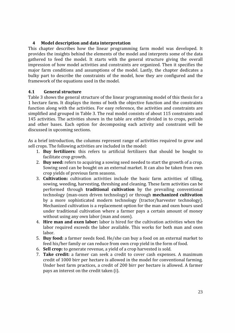
4 Model description and data interpretation
This chapter describes how the linear programming farm model was developed. It
provides the insights behind the elements of the model and interprets some of the data
gathered to feed the model. It starts with the general structure giving the overall
impression of how model activities and constraints are organized. Then it specifies the
major farm conditions and assumptions of the model. Lastly, the chapter dedicates a
bulky part to describe the constraints of the model, how they are configured and the
framework of the equations used in the model.
4.1 General structure
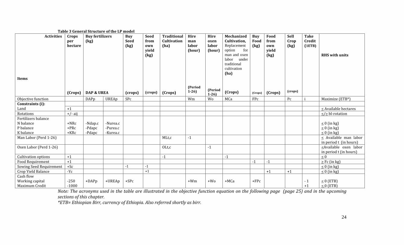
Table 3 shows the general structure of the linear programming model of this thesis for a
1 hectare farm. It displays the items of both the objective function and the constraints
function along with the activities. For easy reference, the activities and constraints are
simplified and grouped in Table 3. The real model consists of about 115 constraints and
145 activities. The activities shown in the table are either divided in to crops, periods
and other bases. Each option for decomposing each activity and constraint will be
discussed in upcoming sections.
As a brief introduction, the columns represent range of activities required to grow and
sell crops. The following activities are included in the model:
1. Buy fertilizers: this refers to artificial fertilizers that should be bought to
facilitate crop growth.
2. Buy seed: refers to acquiring a sowing seed needed to start the growth of a crop.
Sowing seed can be bought on an external market. It can also be taken from own
crop yields of previous farm seasons.
3. Cultivation: cultivation activities include the basic farm activities of tilling,
sowing, weeding, harvesting, threshing and cleaning. These farm activities can be
performed through traditional cultivation by the prevailing conventional
technology (man-oxen driven technology) or through mechanized cultivation
by a more sophisticated modern technology (tractor/harvester technology).
Mechanized cultivation is a replacement option for the man and oxen hours used
under traditional cultivation where a farmer pays a certain amount of money
without using any own labor (man and oxen).
4. Hire man and oxen labor: labor is hired for the cultivation activities when the
labor required exceeds the labor available. This works for both man and oxen
labor.
5. Buy food: a farmer needs food. He/she can buy a food on an external market to
feed his/her family or can reduce from own crop yield in the form of food.
6. Sell crop: to generate revenue, a yield of a crop harvested is sold.
7. Take credit: a farmer can seek a credit to cover cash expenses. A maximum
credit of 1000 birr per hectare is allowed in the model for conventional farming.
Under best farm practices, a credit of 200 birr per hectare is allowed. A farmer
pays an interest on the credit taken (i).
24
Table 3 General Structure of the LP model
Activities
Items
Crops
per
hectare
(Crops)
Buy fertilizers
(kg)
DAP & UREA
Buy
Seed
(kg)
(crops)
Seed
from
own
yield
(kg)
(crops)
Traditional
Cultivation
(ha)
(Crops)
Hire
man
labor
(hour)
(Period
1-26)
Hire
oxen
labor
(hour)
(Period
1-26)
Mechanized
Cultivation, Replacement option for man and oxen labor under traditional cultivation
(ha)
(Crops)
Buy
Food
(kg)
(Crops)
Food
from
own
yield
(kg)
(Crops)
Sell
Crop
(kg)
(crops)
Take
Credit
(1ETB)
RHS with units
Objective function DAPp UREAp SPc Wm Wo MCa FPc Pc i Maximize (ETB*)
Constraints (i):
Land
+1 < Available hectares
Rotations +/- aij </> bl-rotation
Fertilizers balance
N balance
P balance
K balance
+NRc
+PRc
+KRc
-Ndap.c
-Pdapc
-Pdapc
-Nurea.c
-Purea.c
-Kurea.c
< 0 (in kg)
< 0 (in kg)
< 0 (in kg)
Man Labor (Perd 1-26) MLt,c -1 < Available man labor
in period t (in hours)
Oxen Labor (Perd 1-26) OLt,c -1 <Available oxen labor
in period t (in hours)
Cultivation options +1 -1 -1 < 0
Food Requirement +1 -1 -1 > Fc (in kg)
Sowing Seed Requirement +Sc -1 -1 < 0 (in kg)
Crop Yield Balance -Yc +1 +1 +1 < 0 (in kg)
Cash flow
Working capital
Maximum Credit
-250
-1000
+DAPp
+UREAp
+SPc
+Wm
+Wo
+MCa
+FPc
- 1
+1
< 0 (ETB)
< 0 (ETB)
Note: The acronyms used in the table are illustrated in the objective function equation on the following page (page 25) and in the upcoming
sections of this chapter.
*ETB= Ethiopian Birr, currency of Ethiopia. Also referred shortly as birr.

25
Of all the activities in the model, the activity “Sell crop” produces revenue while others
incur costs. The revenue from crop sales minus the costs associated with the required
activities is to be maximized. The constraints associated with the activities are
presented in the rows of table 3. The constraints are explained in the upcoming
sections along with actual data interpretation.
4.2 Explanation of the general structure
Most of the model activities mentioned under section 4.1 are classified per crops. Only
labor related activity is classified on the basis of time. The second column is titled as
“crops per hectare”. It represents the decision variable for the general model. In
section 4.1, the column activities are briefly described. Below, a short description of
the rows in table 3 is presented. Mostly, the rows in table 3 represent the constraints.
• Objective function: it represents revenue (sell crop or Pc) minus the costs. This is
to be maximized. For more details, see section 4.3.
• Land: each crop requires a land to be grown. The sum of land used shall not exceed
the available hectares. For more details, see section 4.5.1.
• Rotations: the crop rotation rules adopted in the model are represented by a host
of crop coefficients. For more details, see section 4.5.2.
• Fertilizer balance: each crop requires a specific NRc, PRc and KRc amount in kg
which is delivered by buying UREA and DAP fertilizers. Each kg of UREA and DAP
bought for each crop contain certain amount or proportion of N (Nurea.c & Ndap.c),
P (Purea.c and Pdap.c) and K (Kurea.c & Kdap.c). These proportions or amounts of
N,P,K in UREA and DAP range between 0 and 1 kg (0% to 100%). For more details,
refer to section 4.5.4.
• Man labor: traditional cultivation requires MLt,c man hours in period to grow crop
C. Man labor can also be hired (-1) in period t. The sum shall be less than the
available man hours in period t. For more details about cultivation activities and
how they are modeled, refer to section 4.5.3.
• Oxen labor: traditional cultivation requires OLt,c oxen hours in period t to grow
crop C. Oxen can also be hired (-1) in period t. The sum shall be less than the
available oxen hours in period t. For more details about cultivation activities and
how they are modeled, refer to section 4.5.3.
• Cultivation options: cultivation (farm activities) can be undertaken through the
traditional (conventional) technology or through the mechanized technology.
Under traditional cultivation, man and oxen labor are mainly utilized (MLt,c and
OLt,c). But when opting for mechanized cultivation, a farmer incurs a
mechanization cost for the farm activities to grow crops (MCa) in replacing the man
and oxen labor that could have been used under traditional cultivation. The
cultivation activities with mechanization option include soil tillage, sowing-
weeding, harvesting, threshing and cleaning. For more details, refer to section 4.5.3.
• Food requirement: the food required in the form of the crops (+Fc) in kg can be
delivered by buying (-1) or by taking from own yield (-1). For more details, refer to
section 4.5.5.

26
• Sowing seed requirement: the sowing seed required to seed the crops (+Sc) in kg
can be delivered by buying (-1) or by taking from own yield (-1). For more details,
refer to section 4.5.4.
• Crop yield balance: Delivered crop yields (-Yc) shall exceed the sum of the seed
from own yield (+1), the food taken from own yield (+1) and crop sold (+1) in kg.
For more details, refer to section 4.5.6.
• Working capital: refers to the season end summary of cash inflows (250 birr
which is the maximum birr amount allowed as a starting working capital and credit
taken (-1)) and cash outflows (buying fertilizers (+DAPp and +UREAp), buying seed
(+SPc), buying food (+FPc), hiring man labor (+Wm), hiring oxen labor (+Wo) and
using mechanized machineries (+MCa) and interest on credit (+1)). There should
be at least a neutral cash balance. Selling crops is another source of cash, but it is
not included in the cash summary. This is because crop yield is sold in the following
agricultural season. For more details, refer to section 4.5.7.
• Maximum credit: represents the maximum of 1,000 birr credit per hectare
allowed. Under best farm practices, 2000 birr per hectare was allowed. For more
details, refer to section 4.5.7.
4.3 The objective function
This model pursues the goal of maximizing the gross farm income from growing
crops. Gross farm income, in this case, is the amount of cash available for a farmer to
expend on his/her personal expenditures like clothing, family bills, etc., investments
or other expenditures Specifically, the gross farm income to be maximized is modeled
as the equation:
Z= ∑c
Pc *YSc - ∑c
DAPp*DAPc -∑c
UREAp*UREAc - ∑c
SPc*SBc
- ∑c
FPc*FBc - ∑t
Wm*HLt - ∑t
Wo*HOt - ∑ca,
MHc*MCa - i
Where:
Z Gross farm income
YSc Yield sold in kg per hectare from Crop C
Pc Farm gate price of crop C in birr per kg
DAPc Amount of DAP fertilizer applied in kg for crop C
UREAc Amount of UREA fertilizer applied in kg for crop C
DAPp Cost of DAP in birr per kg
UREAp Cost of UREA in birr per kg
MLt Number of own man labor in hours utilized in period t
OLt Number of own oxen labor in hours utilized in period t
HLt Number of man labor hours hired in period t
Wm Wage rate per hour for man labor
Hot Number of oxen labor hours hired in period t
Wo Wage rate per hour for oxen labor
MCa Mechanization cost per hectare for cultivation activity a
MHc Amount of hectares under mechanization for cultivation activity ‘a’ per crop C
i Amount of interest paid in birr on credit taken

27
FBc Amount of food bought in kg by a farming family in a season
FPc Cost of food bought in birr per kg
SBc Amount of seed bought in kg for sowing per hectare per crop C
SPc Cost of seed bought in birr per kg
c classification for crops. ‘c’ extends from 1-11, representing 11 crops in the
model
t classification for labor periods. ‘t’ extends from 1-26, representing the two
week periods in one agricultural season
a is a classification for cultivation activities required. ‘a’ represents soil
tillage, sowing, weeding, harvesting, threshing and cleaning.
The definition of gross farm income has already been discussed comprehensively in
chapter 2. The decision variable of this model is the size of acreage (Ac) on which the
different crops are grown. “Ac” can be directly labeled as area of Crop ‘c’ in hectares;
“c” extends from 1-11 incorporating the 11 crops in the model. Most of the items in
the objective function equation have a “c” classification, indicated as crop subscripts.
The labor costs have classification “t” because labor is distributed on a time basis.
Twenty six periods, each comprising two weeks, are used as a basis for developing
labor calendar. Further discussion on the labor periods will be cited more specifically
when we consider the labor constraint. Classifying the items by “c” assists in a clear
decision making from the final results of the model as far as directly relating the
specific costs and revenues to the crops is concerned.
Mechanization cost, which is also a cash expense, is the critical part of the model. It is
the sum of costs associated with hiring a more sophisticated level technology for
executing the farming activities. Mechanization costs (MCa) were classified based on
the range of farm activities required to grow crops since each activity incurs different
levels of mechanization costs. The activity classifications (‘a’) includes soil tillage,
sowing, weeding, harvesting, threshing and cleaning. Apart from these, off-farm
activities such as buying seed and fertilizers can be labeled as input costs. These costs
are mainly incurred out of the pocket of the farmer which is particularly true for
fertilizers. Seed costs are out of pocket cost for the farmer. The farmer can save crop
yields from previous seasons and use them as a sowing seed.
4.4 The Crops
Table 4 below shows some basic information about the crops in Jimma and Ethiopia as
a whole. The crops included in this farm model are chosen based on the significance of
area covered in Jimma. This was especially true for cereals and pulses. For oilseeds,
another criterion apart from area covered such as the opportunity/potential to grow is
used.

28
Table 4 Area and yield in kg/ha of the main crops in Jimma and Ethiopia (Italic are selected crops)
Year 2008/2009
Jimma Ethiopia
Crop Area (*1000)
% Area
(*1000)
%
Cereals 384 87% 8, 770 78%
Teff 134 30% 2481 22%
Wheat 30 7% 1454 13%
Maiz 117 26% 1768 16%
Sorghum 72 16% 1615 14%
Other cereals 31 7% 1451 13%
Pulses 40 9% 1575 14%
Faba Beans 24 5% 538 5%
Field Peas 11 2% 230 2%
Other pulses 5 1% 807 7%
Oilseeds 20 5% 855 8%
Noug 13 3% 313 3%
Linseed 4 1% 181 1%
Soya beans n.a. n.a. 6 .05%.
Sunflower n.a. n.a. 8 .07%
Sesame seed n.a. n.a. 278 2%
Other Oilseed 3 1% 69 .6%
Total grain crops 444 100% 11200 100%
Vegetables, fruits, chat & coffee 117 100% 941 100%
Coffee (within veg, fruits, chat) 72 68% 391 42%
Source: CSA, 2009a, page 43. n.a. information not available
Based on the criterion of area covered in Jimma, the following crops are included in
the model.
Cereals: (maize, sorghum, teff and wheat)
Pulses: (faba beans and field peas)
Oilseeds: (Noug, linseed, soya beans, sunflower and sesame seed)
Soybean is widely recognized as an oilseed, but in some reports, it comes under pulses.
In this case, it is considered as an oilseed crop. Teff, wheat, maize, sorghum and other
cereals covered 87% of the total land area in Jimma. As far as pulses are concerned,
fava bean and field pea shares about 9% of the land. Noug and linseed together
consume the largest oilseed area in Jimma with a share of about 67% of the land
committed to oilseeds. Other oilseeds crops chosen (sesame, soybean, and sunflower)
have a negligible share.
Coffee, which covers a good deal of land (72, 254 hectare) is not included in the model.
Most coffee is merely collected from forest and it is not as labor intensive as the other
crops. Furthermore, coffee is not an instrumental crop in terms of food security. It is
highly a commercial crop. Most of the coffee farms are now under cooperatives and
are being continuously owned by large scale merchants.

29
4.5 Constraints- conventional farm practice
Conventional farm practices refer to the traditional farming style that is predominant
in Ethiopia. This includes farmers that are not in especial government programs and
are not participants of farm experiments being conducted by various agricultural
research institutions.
4.5.1 Land constraint
The most obvious constraint on any farm is probably the area of land available.
Oromiya region’s distribution of agricultural households by holding size in table 5
below assists in determining the size of land that a typical farm possesses. It should be
noted here that Jimma is one of the sub regions within Oromiya region. Land statistics
is only available for Oromiya region.
Table 5 Distribution of Agricultural households by holding size in hectares
Holding size(Ha) No of households
Under 0.1 273,114
0.1- 0.5 852, 682
0.51- 1.00 1, 078, 299
1.01 – 2.00 1, 438, 956
2.01 – 5.00 1,162, 978
5.01-10.00 141, 092
Over 10 10, 544
Total 4, 957, 655
Source: CSA, 2009a
By applying statistical mean calculation for the frequency data, we can arrive at the
average agricultural land size. Using the equation: Mean Xi = ∑ Fi * Mi / ∑Fi, the
calculated average size is 1.72 hectares. This can be rounded off as 2 hectares.
However, to expand the range of results and to analyze the sensitivities of different
farm sizes, the results of various farm sizes will be discussed too. This includes farm
sizes of 1, 5, and 10 hectares. In simple form, the land constraint can be put as:
∑c
Ac + Fallow <= Maximum land Available;
‘Ac’ represents area sown in hectares per each crop. Fallow in this case is part of the
land available which is not exploited for crop cultivation in a certain season of farming.
This land may be reserved for livestock grazing, guarding place and the like.
4.5.2 Rotational constraints
In Ethiopia’s traditional farming, there are a lot of cropping patterns that farmers
exercise and believed to be good for yield and other purposes. About 74.7% of the
crop farmers in Oromiya region reported practicing crop rotation as their main
method of improving soil fertility (CSA, 2009c).

30
Despite of the fact that farmers in Ethiopia practice crop rotation widely, the level of
information they have on the subject is limited. As evidenced in table 4, Ethiopian
farmers in general are only familiar with crop rotation rules that constitute cereals
and pulses. Since a number of oilseeds are included in this model, a new knowledge
framework is required. That is why many of the crop rotation rules in the model are
adopted from guidelines recommended by plant researches and the conventional
practices. For that reason, operational adjustments in applying the results of this
model to the farming practices of the peasants will be necessary. In terms of Ethiopian
calendar, the figure below overviews the seasonal activities with respect to different
crops.
Agricultural activities are highly seasonal in Ethiopia mainly due to the timing of rain.
It is highly critical that crops are sown during the rainy season. Accordingly, a
cropping calendar, which takes approximately 12 months, is divided roughly in to four
(or three) activity seasons: plowing, planting, weeding and harvesting (except that
planting and weeding can overlap and be considered one season). The calendar begins
usually with plowing and the specific timing in the farm calendar depends on the
crops
Figure 4 Crop calendar of Ethiopia
Source: USDA

31
Based on Wijnands et.al. (2011), the following crop rotation rules are adopted in this
model.
1. The same cereal can’t be grown over two successive years
2. After two different cereals are grown, a non-cereal should be grown
3. Faba beans, field peas and soya beans are grown only once every four years
4. A Brassica crop can only be grown once every four years (in the selected set
only applies to noug, commonly known as Abyssinian mustard). A Brassica
crop includes the likes of rapeseed, canola, black mustard, brown mustard and
Asian mustard.
5. Linseed is only grown once in two years
6. Sunflower only once in four years (but no sesame, leguminous or Brassica in
the four year rotation)
7. Sesame is grown only once in four years.
These rules gave rise to 13 specific crop rotation rules. For their formulation and the
corresponding crop coefficients of crops in each rule, see Appendix 5.
These rotational schemes are recommendable rotations that can potentially improve
crop yield and prevent soil nutrient losses. But they are rather prudent set of rotation
rules meaning the rules may be relaxed in practice, but only after sufficient
information has been obtained on practical rotations. For example, in many parts of
the world soya bean is rotated alternatively with maize, so perhaps it should be
allowed to have soybean once every second year. Sunflower has been shown to
perform well after some leguminous crops, so in some USA states crop rotation rules
for sunflower have been relaxed. In these cases, practical data from Ethiopian
experiences are needed to relax the crop rotation rules.
4.5.3 Labor requirement
Human labor
Traditional Ethiopian farming employs both human and animal labor. For simplicity,
all human labor are referred to as manual labor and animal labor are referred as oxen
labor in this model. Oromiya region has an average family size of 4.7 which can be
rounded to a family with 5 members (CSA, 2005). This will serve as the source of
human labor supply. However, not all are economically active. Family members under
the age of 18 are considered as full time students and will only be available for labor
during school breaks.
By breaking down the age structure based on the national age distribution of the CSA,
3 out of 5 members are considered to be economically active all year around. But one
of the 3 members is considered to be not active on the farm, mainly serving as cook
and responsible for other miscellaneous family activities, typically the mother of the
household.
The labor seasons are broken down on a two weeks basis. This means a single
agricultural year will have 26 periods. The labor hours available for all periods are not
constant. In accordance with Ethiopian calendar, periods of school break will have

32
more labor available due to labor of the students in the family. These are six periods
in a calendar they will work on the farm; July 4 – 17, July 18 -31, August 1-14, Aug 15 –
28, Aug 29 – Sept 11, and Dec 19 – Jan 1. These periods supply 288 hours of manual
labor bisected as; 8*6*2*2 + 8*6*2. The first supply (8*6*2*2) represents 192 labor
hours from the two economically active members of the family that work all year
around on the farm. The description of 8*6*2*2 stands for two economically active
family members working 8 hours per day for 6 days for 2 weeks. These 192 hours are
the available labor for the remaining 20 periods of the agricultural calendar. The
additional available labor hours for the six periods(8*6*2) come from school break of
the children who work together in total for 8 hours for 6 days in 2 weeks.
There will be hired human labor when the labor required exceeds the labor supply.
This is true especially for rainy months like June and July that are labor intensive as
the farmers have to plant the crops during this season of the year. The soil tilling
activity is the major agricultural activity during this time for which additional labor is
needed. On the other hand, harvest times like the months of October and November
also need more labor than other months and thus, need hired labor.
Animal labor
Traditional farming also employs a great deal of animal labor. In Ethiopia, oxen are
mainly used for plowing the soil for transporting the harvested crop and threshing.
Donkeys are of great use especially to transport items. Transporting by donkeys can
occur in both conditions of moving harvested crop to threshing area and moving
threshed crop to storage area. Due to the significant use of oxen and other animals,
the labor calendar is developed as done for the manual human labor. But due to the
different type of animals used in different period, it is proper to divide the activities
for farms.
CSA (2009b) indicates renting oxen or pairing with someone else’s ox, particularly for
tilling purpose, is common due to the increasing problem of oxen shortage. In 2009,
852,687 farmers nationally reported renting an ox while 2,821,080 farmers paired
their ox with someone else’s. In Jimma region, 33 % of crop holders had no ox, 30%
had one ox, and 32% had two oxen. Extra oxen hours may be hired in case of labor
deficiency. In this model, it is assumed that a family owns a pair of oxen that work for
8 hours per day for six days providing a constant 192 single oxen hours available in
each period.
The model allows the hiring of labor in each period. The hired labor can be used to
perform any activity that requires manual intervention by man. Below, the
descriptions of essential cultivation activities performed by both man and oxen labor
required for growing the crops are given.
4.5.3.1 General Activities
The general activities are the farm activities that lead up to tilling and some activities
after cleaning. They are considered as activities that are accessory to the main
agricultural activities such as tilling, weeding, harvesting and cleaning. These

33
activities include manure application, land preparation and some parts of
transporting and storage. The activities can be mechanized. But due to their trivial
nature, they are mostly executed manually.
Manure application is one of the minor activities in Ethiopian farming, but considered
important. Organic fertilizer is still widely used in Ethiopia. In 2009, 32% of peasant
holdings used natural fertilizers on cropland areas (CSA 2009c). Animal manure is the
major natural fertilizer on use in Ethiopia. However, thrown food and other garbage
materials are also applied.
Mostly, manure and other materials are dumped on crop lands right after the harvest
of previous season is ended. It is not a labor intensive activity even though it requires
some attention in the follow up. In the model, the four periods after the harvest period
is ended are dedicated to manure application. In each period, 4 hours is given to
manure or other natural fertilizer application. Manual labor by human is the only type
of required labor to undertake manure application (See Appendix 1). In traditional
context, manure application is not supported by any modern machine or the like.
Land preparation is the farm activity before soil tillage. It is also mainly performed by
manual labor without a need for animal labor. After the last harvest, crop lands have
the tendency to grow grasses and unwanted plants. It needs labor intervention to
remove the unwanted plants. The amount of labor hours given to land preparation is
the same for all crops per hectare which is 12 hours (see Appendix 1). Contradictory
to this, it is assumed in the model that the land to be used for farming has been
cultivated.
Finally, transporting and storage refers to the activities after cleaning a harvested
crop. Transporting is related to the human activity required to carry a crop yield from
a farm slot to household’s location for consumption or market place for sales. The
storage is mainly related to the follow up needed to protect any harm to a collected
yield. Some crops require extra care to prevent yield from insects and other sources of
risk (See Appendix 1). Both transport and storage activities could be less or more
labor intensive depending on the amount of the harvest and the care required in
keeping a yield safe.
4.5.3.2 Soil Tillage
Soil tillage is considered a major farming activity in Ethiopia. Ethiopians have a
peculiar way of plowing farm lands which is quite traditional. Almost all peasant
holders make use of a tilling material made from wood. The only metal in the tilling
material is the part that goes in to the ground. It is not an expensive proposition to
obtain it, but the efficiency of the tilling material is far behind the modern machineries
using a tractor. Its inefficiency is mainly related with the huge amount of labor it
consumes to cover a considerable amount of farm field.
Different crops have varying need of soil tillage. Some crops respond only to well-
tilled soil. For instance teff, wheat and some oil seed crops need more tilling than
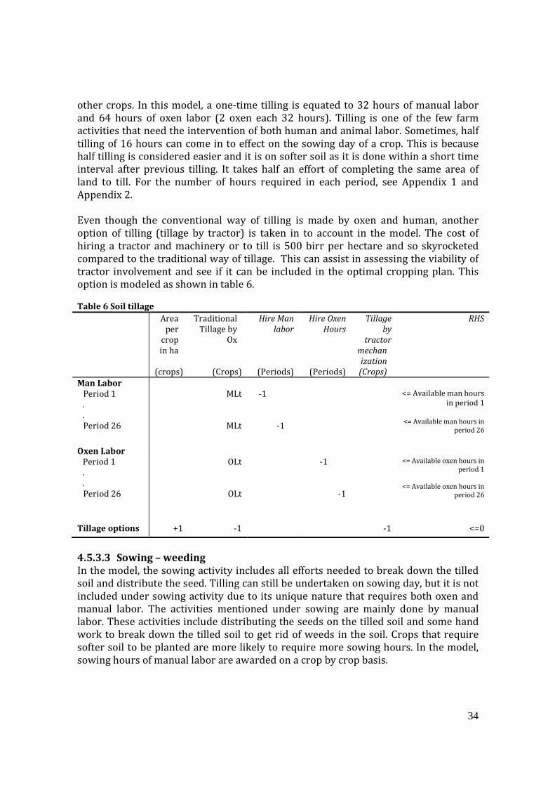
34
other crops. In this model, a one-time tilling is equated to 32 hours of manual labor
and 64 hours of oxen labor (2 oxen each 32 hours). Tilling is one of the few farm
activities that need the intervention of both human and animal labor. Sometimes, half
tilling of 16 hours can come in to effect on the sowing day of a crop. This is because
half tilling is considered easier and it is on softer soil as it is done within a short time
interval after previous tilling. It takes half an effort of completing the same area of
land to till. For the number of hours required in each period, see Appendix 1 and
Appendix 2.
Even though the conventional way of tilling is made by oxen and human, another
option of tilling (tillage by tractor) is taken in to account in the model. The cost of
hiring a tractor and machinery or to till is 500 birr per hectare and so skyrocketed
compared to the traditional way of tillage. This can assist in assessing the viability of
tractor involvement and see if it can be included in the optimal cropping plan. This
option is modeled as shown in table 6.
Table 6 Soil tillage
Area
per
crop
in ha
(crops)
Traditional
Tillage by
Ox
(Crops)
Hire Man
labor
(Periods)
Hire Oxen
Hours
(Periods)
Tillage
by
tractor
mechan
ization
(Crops)
RHS
Man Labor
Period 1
.
.
Period 26
MLt
MLt
-1
-1
<= Available man hours
in period 1
<= Available man hours in
period 26
Oxen Labor
Period 1
.
.
Period 26
OLt
OLt
-1
-1
<= Available oxen hours in
period 1
<= Available oxen hours in
period 26
Tillage options +1 -1 -1 <=0
4.5.3.3 Sowing – weeding
In the model, the sowing activity includes all efforts needed to break down the tilled
soil and distribute the seed. Tilling can still be undertaken on sowing day, but it is not
included under sowing activity due to its unique nature that requires both oxen and
manual labor. The activities mentioned under sowing are mainly done by manual
labor. These activities include distributing the seeds on the tilled soil and some hand
work to break down the tilled soil to get rid of weeds in the soil. Crops that require
softer soil to be planted are more likely to require more sowing hours. In the model,
sowing hours of manual labor are awarded on a crop by crop basis.
35
Nearly all crops in the model require some level of weeding. Weeding mainly
facilitates the growth of planted crops. It can be undertaken either traditionally or in a
modern way. Expectedly in Ethiopia, the traditional way of weeding is predominant.
Traditional weeding is performed by hand which requires only manual labor. On the
other hand, modern weeding is undertaken through the intervention of a tractor.
However, tractor can only come in play if the seeds are planted in rows. This makes it
less likely for Ethiopian case since most farmers use broadcasting of the seeds as a
major sowing technique.
The modeling of both sowing and weeding is the same for how the activity of tillage
was handled. There will be technology option of sowing and weeding by tractor.
However the cost of tractor is different this time. Details of man and oxen labor hours
and costs are provided in Appendix 1, 2 and 6.
4.5.3.4 Harvesting, threshing and cleaning
This farm activity incorporates the range of activities from harvesting of a crop to the
cleaning of harvested crop, leaving the yield to be stored. It represents a highly critical
part of farming in Ethiopia.
After the rainy season is over, the major farming activity of Ethiopia’s agriculture is
harvesting. In the model, harvesting activity refers to broad range of undertakings
involving cutting off or drawing out a crop, preparing the threshing area and
transporting the cut crops to the threshing area. The end of the harvesting activity
marks when the crops are ready to be threshed or cleaned.
The amount of hours required to do these things are again put on a crop by crop basis
(See Appendix 1 and 2). Crops that are tiny and compact in nature tend to require
more harvesting hours. The same is true for threshing and cleaning. Small seeds tend
to consume more hours of threshing and cleaning. In this regard, crops like teff,
sorghum, linseed, wheat and noug will need more labor hours.
Animal labor for threshing may be involved for some crops. However some crops are
delicate to be overrun by animal feet. Hence, the manual and oxen labor may be
combined for some crops and not for other crops. The modeling of these activities is
still consistent as it is portrayed for tilling (See table 6).
4.5.4 Fertilizer and sowing seed requirement and costs
Fertilizer and sowing seed requirements are often regarded as the most direct input
costs for farming. However, the inorganic fertilizers can only be bought. Urea and DAP
are the two most prominent fertilizers bought and applied. The CSA data are used to
derive current fertilizer requirement of N, P and K. Urea and DAP use have been
converted to N and P using (0.46 N per kg urea and 0.46 P per kg DAP). K-requirement
was calculated from exported K in seed (= seed yield x K-content in seed) and using a
recovery of 70 % of K-applied. The specific nutrient amount required for each crop
and other details are provided in Appendix 4. The cost of DAP and UREA were directly

36
adopted from the fertilizer market in Ethiopia. DAP costs 2.55 birr per kg while UREA
costs 2.5 birr per kg (CSA, 2009c).
As indicated, sowing seed can either be bought on the market or taken from previous
yields. The cost of sowing seed on the market is derived from the farm gate prices of
each product. It is assumed that the sowing price is higher than the farm gate price.
This is due to two reasons. First, the sowing season is usually at the time of low supply
of crop yields on the market. Secondly, there will be additional cost of storing added to
the farm gate price which is incurred between time of harvest and the season of
sowing. Thus, the seed price is assumed 1.5 times the farm gate price and 3 times in
the case of best farm practice. Table below shows the farm gate and the sowing seed
price of each crop.
Table 7 Farm gate and Seed Price of the crops
birr/kg Birr/kg Birr/kg
Crops Farm gate
price
Seed Price
(Conventional farming
Seed Price
(Best farm practices)
Teff 6.0 9.0 18.0
Wheat 5.0 7.5 15.0
Maize 3.5 5.3 10.5
Sorghum 3.5 5.3 10.5
Faba 4.8 7.2 14.4
Fieldpea 5.3 7.9 15.9
Soya 4.0 6.0 12.0
Noug 5.5 8.3 16.5
Linseed 5.0 7.5 15.0
Sunflower 5.3 7.9 15.9
Sesame 8.0 12.0 24.0
4.5.5 Food requirement
Food security is one of the greatest challenges faced by Ethiopian farmers in general.
Historically, the region of Jimma has not encountered a big problem in feeding its
people. One of the major purposes of this model is to make sure that there is a
condition set that ensures there is at least a minimum food available for the family.
The farmer’s family uses most of all produced agriculture products for own
consumption.
Own produced goods will be the main source for consumptions. Figure 5 shows the
share of own use on the average farm. Of the cereals and pulses over 80% is used for
either consumption or sowing seeds. Of oilseeds, 65% is used for these purposes.
Cereals are the most important food crops, the production amounts 145 million tons,
pulses are the second (20 million tons). The quantity of oilseeds (7 million tons) is a
mere 5% of the cereal production. Neug, sesame seed, rapeseed, beef and eggs are
mainly sold, providing the farmers cash. In conclusion, the major part of the crops is
consumed on the own farm.

37
Figure 5 Percentage utilized of production in 2008/2009 (2001 E.C.)
Source: Wijnands et al., 2011.
Based on the above distribution the amount food consumed in kg by a typical family is
calculated in a way portrayed in table 8:
Table 8 Food consumption computation
Produced
*1000
Consumed Amount
consumed
per head
consumed
Family
Consumption
Crops
(tons/year) ( %) (tons/year) (Kg/year) (Kg/year)
Cereals
Teff
1,508
67
101,050
46
230
wheat 464 58 26,912 12 61
maize 3,097 75 232,310 105 528
sorghum 1,230 77 94,731 43 215
Pulses
Faba 276 55 15,226 7 35
Field 109 55 6,008 3 14
Soya 1 0 0 0 0
Oilseeds
Nueg 53 53 2,846 2 10
linseed 20 32 668 1 5
sunflower 1 0 0 0 0
sesame 12 0 0 0 0
The last column in the column above represents the food required per crop for a
family to survive (Fc, see table 3). In the model, “FOc” is the amount of food consumed
0
10
20
30
40
50
60
70
80
90
100Cereals
Pulses
Oilseeds
Neug
Linseed
Sesam
e
Rapeseed
Milk
Butter
Cheese
Beef
Mutton/Goat
Eggs
Chicken
Own consumption Seed Sale Other

38
from own yield per year per family. The farmer can still buy food from outside but at a
price (FBc) of 1.25X the farm gate price. In essence, this can be put as:
- FOc - FBc >= Fc (See table 3)
4.5.6 Crop yield balance
The yield of each crop goes through various deductions before the final balance is
reached. Appendix 3 shows the input requirements that transact within the yield
balance. The seed consumption from own yield, food consumption from own yield and
amount of yield sold represent the deductions from the crop yields. These deductions
shall not exceed the actual yield of a crop. These transactions can be converted in to
an equation model that looks like:
-Yc + Soc + SBc + YSc <= 0 (See table 3)
Where:
Yc Actual yield in kg per hectare from crop C
SOc Amount of own seed used for sowing with zero cost per crop C
FOc Amount of own food consumed with zero cost per crop C
YSc Amount of yield sold in kg per crop C
4.5.7 Cash flow requirement
Cash flow is a summary of projected cash inflows and cash outflows for a business
over a given period (Ronald et al, 2008). It is desired in this model that a particular
farm has at least a neutral cash balance. This requirement, which is explained in the
equation below, captures all the cash receipts and cash expenses covered in this
model for all the periods that have an impact on the working capital.
Besides, a maximum starting working capital of 250 birr per hectare and a maximum
credit of 1000 birr per hectare are allowed. These two provisions are the sources of
cash which serve as the first amount of cash a farmer needs before growing the crops.
The other cash source is the sales from crop yields. The working capital balance
equation in the model can be put as:
WC = - SC*FS – C*FS +∑c
DAPp*DAPc + ∑c
UREAp*UREAc + ∑c
SPc*SBc
+ ∑c
FPc*FBc + ∑t
Wm*HLt + ∑t
Wo*HOt + ∑ca,
MHc*MCa + i <= 0 (see table 3)
Where:
WC The working capital balance of a farmer in a season.
SC Starting working capital allowed for a farmer in a season per hectare
FS Available farm size in hectares
C Amount of money borrowed in birr by a farmer in a season per hectare
YSc Yield Sold in kg per crop C
Pc Farm gate price of Crop C in birr per kg
DAPa Amount of DAP fertilizer applied in kg
UREAa Amount of UREA fertilizer applied in kg
DAPp Cost of DAP in birr per kg

39
UREAp Cost of UREA in birr per kg
HLt Number of manual labor hours hired in period t
Wm Wage rate per hour for manual labor
Hot Number of oxen labor hours hired in period t
Wo Wage rate per hour for oxen labor
MCa Mechanization cost per hectare for cultivation activity a
MHc Amount of hectares under mechanization for a cultivation activity per crop C
i Amount of interest paid in birr on credit taken
FBc Amount of food bought in kg by a farming family in a season
FPc Cost of food bought in birr per kg
SBc Amount of seed bought in kg for sowing per crop C
SPc Cost of seed bought in birr per kg
4.6 Best farm practices
The second major farm situation considered in this model is the best farm practices.
Best farm practices refer to the farmers involved in especial government programs
and follow specific scientific recommendations of farm research institutions. This
practice usually results in higher yields, but at high costs and resource consumption.
(See table 9)
The framework of equations for best farm practices and the conventional farm
practices are the same. However, the coefficients may differ. Table below summarizes
the differences from the conventional farming.

40
Table 9 Major differences between the two farm practices.
Item Best farm practice Conventional farm practices
Seed Improved seed varieties are sown under best
farm practices. The seeds can only be
purchased from a special seed market at an
expensive rate. In this model, the seed price is
assumed 3X the normal farm gate value of the
crops.
Purchase of seed at 1.5X farm
gate value is allowed or seed
is taken from own yield.
Human
Labor
The number of human hours needed under best
farm practice is greater due to extra human
intervention needed. Extra labor hours are
required for three reasons. First, an extra
tillage is required in best farm practices as the
soil has to be softer. Second, higher yields mean
greater number of harvest, threshing and
storage hours. Third, extra care and
supervision of crops is required under the best
farm practices.
Human labor hours are
calculated for different farm
activities based on the
specific crop requirement for
each activity.
Oxen
Labor
Oxen labor hours will also be greater. An extra
soil tillage and threshing under best farm
practices means more oxen hours.
Oxen labor hours are
calculated in the same way
for human labor hours
Fertilizer Specific scientific recommendations of fertilizer
to achieve maximum yields under the
circumstances are adopted.
The fertilizer consumption is
based on the CSA data.
Credit A credit of 2000 birr per hectare is allowed.
The amount allowed is higher than under the
conventional practices because of the fact that
more cash expenses are required. Fertilizer and
seed cost is by far greater under the best farm
practices.
A credit of 1000 birr per
hectare is allowed under the
conventional farming.
Yield Special program yields adopted from farm
research institutes. These yield figures are
typically higher than the yields of conventional
farming.
Actual yields recorded based
on CSA data
Crop
protection
expense
Crop protection expense exists under best farm
practices. It is a unique cost incurred to give
extra care and follow up for the growing crops.
Crop protection expense does
not exist under conventional
farming.

41
4.7 Summary information of crops
The two tables below summarize the prominent input information for the crops in the
model. The nominal gross margin before optimization is computed for each crop. It is
calculated as:
GMc = Yc*Pc – DAPc*DAPp – UREAc*UREAp – Sc*(Pc*k)
Where
GMc Gross margin per hectare of crop C
Yc Actual yield per hectare in kg from crop C
Pc Farm gate price of Crop C in birr per kg
DAPa Amount of DAP fertilizer applied in kg per hectare
UREAa Amount of UREA fertilizer applied in kg per hectare
DAPp Cost of DAP in birr per kg
UREAp Cost of UREA in birr per kg
Sc Amount of seed required per hectare to grow crop C
k Cost multiplier for seed cost. As discussed, ‘k’ is 1.5X the farm gate price
for conventional farming and 3X for best farm practices.
In short, the gross margin is estimated as sales from a crop yield minus the fertilizer
and seed costs. Fertilizer and seed as discussed above are the major input costs for
which a farmer expends cash by buying items from an external market. It gives some
indications on how a given crop is financially attractive.
Table 10 Crop summary under conventional farm practices
Crops Gross
margin
Birr/ha
Man’l
labor
Hrs/ha
Oxen
labor
Hrs/ha
Actual
Yield
Kgs/ha
Farm
price
Birr/kg
DAPc
Kg/ha
UREAc
Kg/ha
Seed
rate
Kg/ha
teff
wheat
maize
sorghum
faba
fieldpea
soya
noug
linseed
sunflower
sesame
5473
5532
6506
4596
3438
4008
4374
2233
2353
3546
4974
556
496
324
396
380
332
452
388
420
322
300
506
360
200
272
184
184
240
260
212
248
184
1000
1400
2000
1500
1000
1000
1200
450
550
700
650
6
5
3.5
3.5
4.8
5.3
4
5.5
5
5.3
8
60
72.5
85
25
50
50
35
22.5
35
12.5
25
120
145
170
50
100
100
70
55
70
25
50
30
175
15
120
185
150
50
15
35
10
10
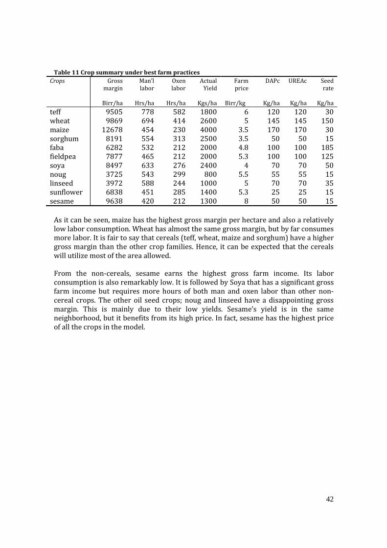
42
Table 11 Crop summary under best farm practices
Crops Gross
margin
Birr/ha
Man’l
labor
Hrs/ha
Oxen
labor
Hrs/ha
Actual
Yield
Kgs/ha
Farm
price
Birr/kg
DAPc
Kg/ha
UREAc
Kg/ha
Seed
rate
Kg/ha
teff
wheat
maize
sorghum
faba
fieldpea
soya
noug
linseed
sunflower
sesame
9505
9869
12678
8191
6282
7877
8497
3725
3972
6838
9638
778
694
454
554
532
465
633
543
588
451
420
582
414
230
313
212
212
276
299
244
285
212
1800
2600
4000
2500
2000
2000
2400
800
1000
1400
1300
6
5
3.5
3.5
4.8
5.3
4
5.5
5
5.3
8
120
145
170
50
100
100
70
55
70
25
50
120
145
170
50
100
100
70
55
70
25
50
30
150
30
15
185
125
50
15
35
15
15
As it can be seen, maize has the highest gross margin per hectare and also a relatively
low labor consumption. Wheat has almost the same gross margin, but by far consumes
more labor. It is fair to say that cereals (teff, wheat, maize and sorghum) have a higher
gross margin than the other crop families. Hence, it can be expected that the cereals
will utilize most of the area allowed.
From the non-cereals, sesame earns the highest gross farm income. Its labor
consumption is also remarkably low. It is followed by Soya that has a significant gross
farm income but requires more hours of both man and oxen labor than other non-
cereal crops. The other oil seed crops; noug and linseed have a disappointing gross
margin. This is mainly due to their low yields. Sesame’s yield is in the same
neighborhood, but it benefits from its high price. In fact, sesame has the highest price
of all the crops in the model.

43
5 Results of the model
This chapter will concentrate on the presentation and explanation of the main results of
the model. The results to be discussed include model validation, the optimum cropping
plan, the revenues and expenses, and the sensitivity analysis. These results are
organized on the basis of farm sizes and farm practices. Farm size is chosen to analyze
the effect of changes in farm sizes. Results will be presented for farm sizes of 1, 2, 5 and
10 hectares. Farms larger than 10 hectares are usually commercially owned and do not
reflect peasant farming. Additionally, results will be presented and discussed for two
kinds of farm practices: conventional and best farm practices.
5.1 Validation of the model
This section evaluates the consistency of the optimization model with the actual farm
practice of the region. The previous chapter has described how farm realities of the
region are molded in to the model. But models rarely reflect the real situation perfectly.
Hence, there are some major settings of the GAMS model that deviate from the pure
reality.
To quantify the effect of these inconsistencies, table 12 below compares the results of
the actual cropping plan with the optimal cropping plan results for a farm size of 1.72
hectares. The average farm size in Ethiopia is 1.72 hectares. The table also gives the
revenue and expense details of each plan along with the minimum farm size of each
crop that is needed to meet the food demand of the family. The minimum farm sizes
indicated in the last column are crop land sizes that should be grown to avoid buying
food from external market. If the size of any crop falls short of the prescribed
minimum in the cropping plan, there will be food expense which is bought from
external market.
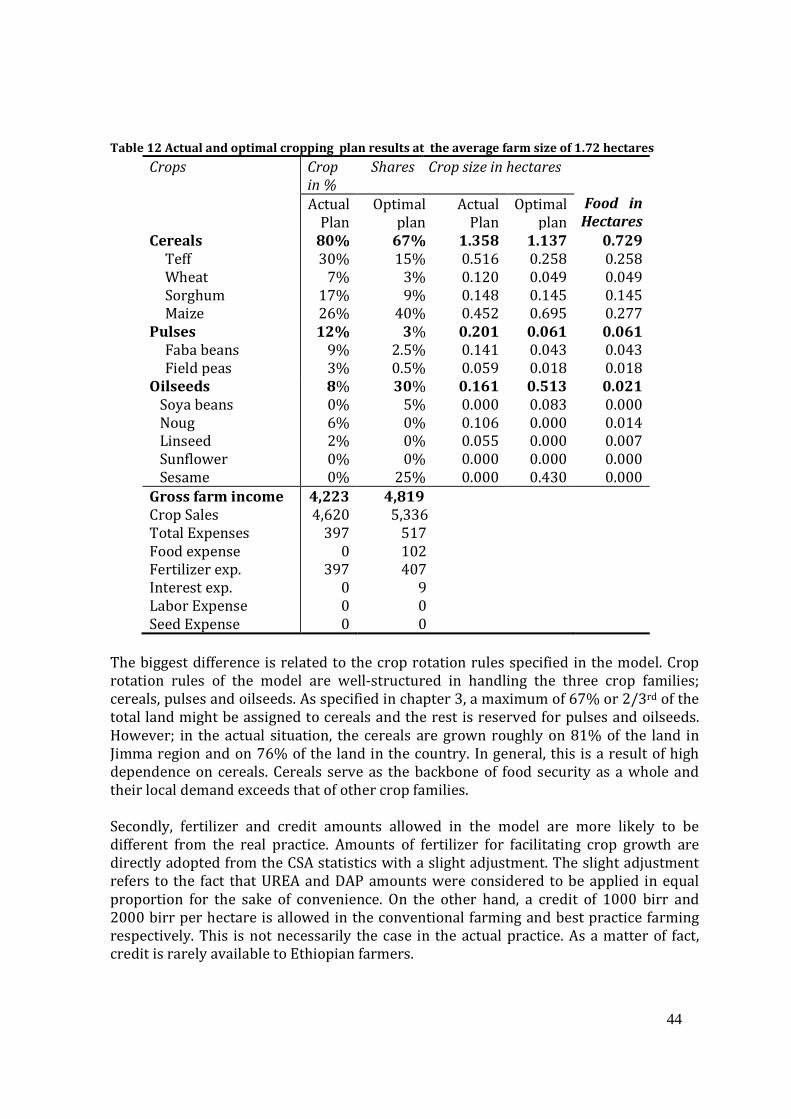
44
Table 12 Actual and optimal cropping plan results at the average farm size of 1.72 hectares
Crops Crop Shares
in %
Crop size in hectares
Food in
Hectares Actual
Plan
Optimal
plan
Actual
Plan
Optimal
plan
Cereals
Teff
Wheat
Sorghum
Maize
80%
30%
7%
17%
26%
67%
15%
3%
9%
40%
1.358
0.516
0.120
0.148
0.452
1.137
0.258
0.049
0.145
0.695
0.729
0.258
0.049
0.145
0.277
Pulses
Faba beans
Field peas
12%
9%
3%
3%
2.5%
0.5%
0.201
0.141
0.059
0.061
0.043
0.018
0.061
0.043
0.018
Oilseeds
Soya beans
Noug
Linseed
Sunflower
Sesame
8%
0%
6%
2%
0%
0%
30%
5%
0%
0%
0%
25%
0.161
0.000
0.106
0.055
0.000
0.000
0.513
0.083
0.000
0.000
0.000
0.430
0.021
0.000
0.014
0.007
0.000
0.000
Gross farm income
Crop Sales
Total Expenses
Food expense
Fertilizer exp.
Interest exp.
Labor Expense
Seed Expense
4,223
4,620
397
0
397
0
0
0
4,819
5,336
517
102
407
9
0
0
The biggest difference is related to the crop rotation rules specified in the model. Crop
rotation rules of the model are well-structured in handling the three crop families;
cereals, pulses and oilseeds. As specified in chapter 3, a maximum of 67% or 2/3rd of the
total land might be assigned to cereals and the rest is reserved for pulses and oilseeds.
However; in the actual situation, the cereals are grown roughly on 81% of the land in
Jimma region and on 76% of the land in the country. In general, this is a result of high
dependence on cereals. Cereals serve as the backbone of food security as a whole and
their local demand exceeds that of other crop families.
Secondly, fertilizer and credit amounts allowed in the model are more likely to be
different from the real practice. Amounts of fertilizer for facilitating crop growth are
directly adopted from the CSA statistics with a slight adjustment. The slight adjustment
refers to the fact that UREA and DAP amounts were considered to be applied in equal
proportion for the sake of convenience. On the other hand, a credit of 1000 birr and
2000 birr per hectare is allowed in the conventional farming and best practice farming
respectively. This is not necessarily the case in the actual practice. As a matter of fact,
credit is rarely available to Ethiopian farmers.

45
Last but not least, labor planning of the model is more scientific and efficient than the
actual farm practice. To assume that labor can be hired whenever the family labor falls
short of the demands in some way overlooks the difficulties. In addition to this, the wage
of labor hiring may be volatile based on the type of activity or the time in the labor
calendar. For example, labor for harvesting may cost more than labor for soil tillage
because it requires higher skill.
The points mentioned above are the major inconsistencies that can be attributed to
the fact that the model represents only some parts of the farm reality in Ethiopia. The
most important difference between the two plans as noted above is with regard to the
crop rotation scheme. As it can be seen, cereals have a significant share in the actual
crop growing practice of the region. Teff, wheat, sorghum and maize were grown over
80% of the land in the actual plan while they consumed the maximum allowed 67% of
the land in the optimal plan. Teff and maize in particular have high shares in the actual
plan with 30% and 26% of the land respectively. These two crops in combination
consume more than half of the land available. As evidenced in the last column of the
table, 0.258 and 0.277 hectare of teff and maize respectively are required to meet the
food demand of these two crops. This clearly shows that teff and maize are the two
most prominent crops used for food consumption in the region.
There will be yield available for sale for both maize and teff since the hectares in the
actual plan (teff=0.516 and maize=0.452) are greater than the hectares needed for
family food. However; in the optimal plan, even if both maize (40%) and teff (15%)
have a great share of the land, but most of the land went to maize because of its high
gross farm income. Under the optimal plan, teff is grown over the minimal land
required for food. This indicates maize is available for sale, but not teff.
Another major crop which is available for sale in the optimal plan is sesame with
0.430 hectares in the optimal plan and with zero hectare required for food. Same
explanation can be made for soya bean. In fact, the biggest difference between the two
plans in terms of oilseeds is related to the role of soya bean and sesame. Soya and
sesame have a negligible share in the actual plan. But these two crops utilize 29% of
the land as far as the optimal cropping plan is concerned. In the actual plan, it is noug
and linseed with a share of 8% of the land that represents the participation of oilseeds.
Unfortunately, both suffer from a lower gross farm income as shown in the summary
crop information in chapter 3. Crops can be included in the actual plan even if they
have a low gross farm income since their land sizes are predetermined based on the
overall farm practice of the region. This shows noug and linseed are the two most
commonly grown and consumed oilseed crops, which is evidenced by the minimum
size of land (0.014 and 0.007 hectares) needed in the food column.
On the other hand, the crop sizes in the optimal plan are not as predetermined as they
are in the actual plan. The guiding factor for the optimal plan in determining the land
size of crops is the minimum food requirement in hectares. However, under
optimization, the plan can flexibly avoid growing some crops that do not have high

46
gross farm income to be purchased and use the land left for growing more crops with
a better gross farm income figures. This flexibility is proven especially for the cereals
and oilseeds. Under cereals, maize has the highest gross farm income. Thus the other
cereals (teff, wheat and sorghum) are only grown at 0.258, 0.049 and 0.145 hectares
respectively so that the rest of the land available goes to maize.
This adjustment allows growing maize over 0.695 hectares. The indicated size is the
maximum land size maize can have, mainly due to the crop rotation restriction that
assigns 67% of the land to cereals. Assessing the oilseed participation under the
optimal plan, the minimum land required for nueg and linseed is not met. This is
because purchasing these crops from the external market and transferring these
minimum land requirements to two other oilseed crops, soya bean and sesame has a
more favorable impact on the gross farm income. The optimal plan does not include
purchasing pulses (faba and field peas) from the external as evidenced by the land
required which are 0.043 and 0.018 hectares respectively.
Hence, the amount of land saved from not growing nueg and linseed and from
growing faba and field pea went to sesame and soya bean. The first land allotment
went to sesame and as a result, 0.430 hectares of sesame was grown. This is 25% of
the land which is the maximum allowed share for an oilseed. The second most
attractive crop financially was soya bean and the rest of the land went to it. As a result,
soya bean is grown over 0.083 hectares of land grown. This flexible land adjustment is
the primary reason behind the better gross farm income figures under the optimal
cropping plan.
Breaking down the details of the expenses, food expense in the actual plan are zero,
but 102 birr in the optimal plan. The food expense in the optimal plan is not consistent
with the actual situation. As seen in table 12, the actual plan covers all the crop size
required to meet the food demand. The optimal plan doesn’t meet those requirements
for noug and linseed since they are not included in the optimal plan. Thus, the 102 birr
expense is directly related with purchasing noug and linseed from the food market. As
a result of this change, the sales of the optimal plan are much higher than while the
costs of the actual plan are lower. Fertilizer costs are only a little higher. So the
difference in the costs is mainly explained by the possibility of food expenses.
5.2 Conventional practice results This section presents the optimization results of the model for the conventional farm
practices. Conventional farm practices refer to the traditional farming style that are
predominant in Ethiopia. This includes farmers that are not in especial government
programs and are not participants of farm experiments being conducted by various
agricultural institutions.
5.2.1 Optimum plan results Table 13 presents the three types of key results of conventional farm practices. First,
it shows at different farm sizes the optimal cropping plan in hectares with the
respective percentages along with minimum crop size required to meet food demand.

47
Secondly, it summarizes the revenues, expenses and the gross farm income as a result
of the optimal crop plans. Thirdly, it summarizes the status of major resources in the
model.
Table 13 Optimal cropping plan and economic results for conventional farm practices at
different farm sizes
*Both man and oxen labor are fully used only in some periods. Note that the expression
‘fully used’ is a short expression for ‘fully used in some periods’.
The cropping plan distribution is more or less the same for all farm sizes except for 1
hectare. As expected, maize takes the highest share in all optimum cropping plans. For
all farm sizes bigger than 2 hectares, 50% of the land is assigned to maize which is the
maximum allowed land. In the 1 hectare land distribution, maize is grown on only
0.277 hectares which is equal to the minimum land size required to meet food
demand. This shows maize is not sold for generating revenue. This in turn indicates 1
hectare is too small to satisfy the food demand of the family and have an extra land
available for the crops with an attractive gross farm income. This, for instance, is
clearly witnessed by the crop size of cereals. The size of all cereals except sorghum
were only able to meet the minimum required food size. Teff, maize, and wheat only
were grown over 0.258, 0.049 and 0.277 hectares respectively, equal to the hectares
Crop 1 ha % 2 ha % 5 ha % 10 ha % Food in
hectares
Cereals
Teff
Wheat
Sorghum
Maize
Pulses
Faba
Field pea
Oilseeds
Soya
Noug
Linseed
Sunflower
Sesame
0.258
0.049
0.083
0.277
0.043
0.018
0.023
0.000
0.000
0.000
0.250
67
25.8
4.9
8.3
27.7
6
4.3
1.8
27
2.3
0.0
0.0
0.0
25
0.258
0.049
0.145
0.882
0.043
0.018
0.106
0.000
0.000
0.000
0.500
67
12.9
2.4
7.2
44.1
3
2.1
0.9
30
5.3
0.0
0.0
0.3
25
0.258
0.431
0.145
2.500
0.043
0.018
0.656
0.000
0.000
0.000
0.950
67
5.2
8.6
2.9
50
1.5
0.9
0.4
32
13
0.0
0.0
0.0
19
0.258
1.264
0.145
5.000
0.043
0.018
1.892
0.000
0.000
0.000
1.381
67
2.6
12.6
1.5
50
0.6
0.4
0.2
32.7
18.9
0.0
0.0
0.0
13.8
0.729
0.258
0.049
0.145
0.277
0.061
0.043
0.018
0.021
0.000
0.014
0.007
0.000
0.000
Resource Use
Land
Own Man Labor
Own Oxen Labor
Credit
Fully used
Not fully used
Not fully used
Used
Fully used
Not fully used
Not fully used
Used
Fully used
Not fully used
Fully used*
used
Fully used
Fully used*
Fully used*
used
Revenues & Expenses
Gross farm income
Crop Sales
Total Expense
Food Expense
Fertilizer Expense
Interest Expense Labor expense (Man)
Labor Expense (Ox)
Seed Expense Gross farm income per ha
605
1385
780
501
226
53 0
0
0
605
6, 435
7, 030
595
102
484
10 0
0
0
3,218
23, 457
24, 851
1,394
102
1,199
14 0
79
0
4,691
50,379
54, 296
3,917
102
2,285
142 382
996
0
5,038

48
of food. Sorghum was grown over 0.083, which is even less than the minimal size
required (0.145 hectares). This means yield of sorghum equivalent to 0.06 hectares
will be outsourced or purchased. The sum of the size of cereals mentioned under the 1
hectare plan above is 0.667 hectares. This sum has already reached the maximum
allowed land for cereals, i.e., 67%.
Hence, it is not possible to grow maize beyond the minimum requirement, which
negatively influenced the gross farm income for the 1 hectare plan. The absence of
crop sales with high gross farm income like maize clearly indicates the impact of
having a small farm size. There is no particular crop with a very high share of the land
under 1 hectare and as seen in the resource usage status, land is the only resource
that is fully utilized. The critical resource shortage explains the uncharacteristically
low gross farm income per hectare, shown on the last row. The gross farm income per
hectare increased dramatically from 605 to 3,218 birr after increasing farm size to 2
hectares.
Soya bean and sesame are the only two crops that will be sold under 1 hectare plan.
Soya bean and sesame are not needed for food and yet have a share in the optimal
plan. Thus, all of their yield will be used for sales. Nueg and linseed are not grown for
economic reasons while the pulses (faba=.043 hectares, field pea=0.018 hectares) are
grown to meet the minimal food requirement. The extra land available from these
distributions went to sesame and soya bean. The first land allotment was attributed to
sesame until it reached the maximum land share allowed (25%), then a tiny amount of
land (0.023 hectares) went to soya bean.
In the 2, 5 and 10 hectare plans, share of maize is greater than 0.277 hectares. Hence,
there is maize available for crop sales. Wheat is sold in 5 and 10 hectare optimal plans,
but not at the 2 hectare plan. Other cereals (Sorghum and Teff) had a contribution in
the optimal plans that are only sufficient to meet the food demand. The advantage of
having bigger farm sizes such as these is the possibility of extra land available for
growing crops with high gross farm income over large land sizes. This boosts the crop
sales significantly. The sum of minimum land required for food under cereals is 0.729
hectares (the sum of 0.258, 0.049, 0.145 and 0.277 hectares). For example, under the
5 hectare crop plan, 67% of the land (3.35 hectares) is available to be utilized by
cereals. Thus, there will be a big chunk of land to go beyond the minimum
requirements. In doing so, priority is given to crops with high gross margin (See table
10). As a result, the share of maize was increased until the maximum allowed
land(50%) is reached. Growing wheat above the minimum land size required was
even possible at the 5 hectare plan as it has a share of 0.431 hectares. This analogy is
also true for the 10 hectare plan.
With regard to oilseeds, soya bean and sesame has almost the same role in the 2,5 and
10 hectare plans. In general, cereals have consumed the maximum allowed land
proportion, i.e., 67%. Out of what is left for other crops that are not cereals, most of
the land is consumed by sesame and soya bean. Sesame and soya bean shared more
than 30% of the land between themselves. In the case of all farm sizes, soya bean and

49
sesame had a share of more than 25% of the land. As discussed under the 1 hectare
plan, nueg and linseed were purchased and pulses (faba beans and field peas) were
grown at their minimal level, leaving a substantial land to be utilized by sesame and
soya bean.
Land is a limiting factor for all farm sizes. This indicates land is the only resource in
the model limiting the gross farm income in all the cases. Oxen labor becomes a
binding factor for some periods with labor shortages for farm sizes greater than 5,
while human labor becomes limiting only after 10 hectares and beyond. This shows
oxen labor has higher economic value and is more scarce than the human labor. It is
important to note that labor shortage is not faced in all periods. Labor will always be
idle in some periods. It is only in peak periods like period 7 (see Appendix 1 and 2)
that labor is fully used and hiring is needed. Additionally, credit is used in all farm
sizes, but in all cases, the maximum allowed credit is not reached. Hence, credit is a
critical resource of the model, but not binding.
Assessing the revenue and expense figures, food cost is the highest cost incurred for
the 1 hectare size and it is the only case where the food cost exceeded the fertilizer
cost. In fact, food cost of 501 birr under the 1 hectare plan is larger than the other
observed food costs of 102 birr for the other farm sizes. The reason behind the high
food cost under 1 hectare relates to the inclusion of sorghum in the food purchase. In
all farm sizes except 1 hectare, noug and linseed are the only two crops that are not
grown meet the food demand and need to be purchased. But under 1 hectare, share of
sorghum, noug and linseed are not sufficient for food demand. Thus, these three crops
are purchased from the market to keep the family from food insecurity.
Fertilizer expense is directly related with the farm sizes. The expense doubled as farm
size is increased from 1 to 2 hectare and from 5 to 10 hectares. There is no labor
expense until 5 hectare is reached. And the first labor type that was fully utilized and
hired was an oxen labor. Thus, the 79 birr labor expense in relation to the 5 hectare
crop plan resulted from oxen hiring. Under 10 hectares, there is a significantly high
labor expense. Both man and oxen labor were hired. That is why interest expense was
much higher form the rest of the farm sizes as cash was needed for compensation.
The food expense explains the change in the gross farm income from 1 to 2 hectares.
The food expense decreases dramatically. Besides, the 1 hectare farm size has proven
to be small to provide a significant amount of crop yields for sales. Hence the crop
sales per hectare was significantly larger under 2 hectares(3,015 birr) , compared to 1
hectare (1,385 birr).
The gross farm income per hectare increased by 1473 birr moving from 2 to 5
hectares while it jumped by only 347 birr in shifting from 5 to 10 hectares. There are
two factors in the increase moving from 2 to 5 hectares. The first one is due to the
simple reason that the food expense stayed the same. Food expense was 102 birr for
both farm sizes. Thus the same cost for two different farm sizes means a lower cost
per hectare for the larger farm size. The other reason was the increase in sales per

50
hectare. Crop sales per hectare under the 2 hectare plan is 3, 015 while it is 4, 970
under the 5 hectare plan. These two combinations caused the higher gross farm
income per hectare. The increase in gross farm income per hectare in moving from 5
to 10 hectares is also explained by these two factors. But there were other reasons
that contributed for the low increase (347 birr). First, the farm size more than
doubled in shifting from 2 to 5 hectares. This gives it more advantage. Secondly, even
if the crop sales per hectare boomed from 4,970 birr to 5,430 birr, the need for more
cash due to more labor expenses increased the interest expense and the labor expense
per hectare by more than 10 times. Labor expense was higher since the labor available
(the family size) stayed the same as the farm sizes increased.
5.2.2 Sensitivity analysis Sensitivity analysis was done in order to capture the effects of major variables. It is
one of the several measures to evaluate how representative a model is (Kruseman,
2000). This section will outline the changes in the optimal results by altering the
status of variables such as farm gate price, labor availability and credit level. Two
kinds of sensitivities were undertaken. The first is price changes for both inputs and
outputs in the model. Variation in price of some crops and changes in costs of labor
are included in this division. The second type is change of constraint. The effects of
either relaxing or making some constraints more strict will be discussed.
The 5 hectare solution report will be used as a basis for comparisons. This farm size is
chosen for two reasons. First, it is large enough to clearly indicate the effect of some
variables. For instance, the effect of decreasing labor availability doesn’t come in to
play until 5 hectare farm size is reached. Secondly, 5 hectare can be used as a typical
cropping plan distribution. The cropping plan of 5 hectares is nearly uniform with all
the plans greater than 2 hectares.
5.2.2.1 Increase in price of soya bean and sunflower
Table 14 presents how the optimal cropping plan changes with the increase in price of
Soya beans and Sunflower. With the increasing international market demand and the
possible diversification of food sources in Ethiopia, it is foreseeable that their price
will go up. So the question to be answered is how far their prices should be increased
until their share reaches maximum allowed land. The price will be increased by 0.5
birr step by step.

51
Table 14 Price* increase impacts of soya bean and sunflowers at the 5 hectare conventional farm
Crop Base Increase
by 0.5
birr
Increase
by 1.00
birr
Increase
by 1.5
birr
Crops
Cereals
Teff
Wheat
Sorghum
Maize
Pulses
Faba
Field pea
Oilseeds
Soya
Noug
Linseed
Sunflower
Sesame
Revenues and Expenses
Gross farm income
Crop Sales
Total Expense
Food Expense
Fertilizer Expense
Interest Expense
Labor Expense (man)
labor Expense (ox)
Seed Expense
67%
0.258
0.431
0.145
2.500
1.2%
0.043
0.018
32%
0.656
0.000
0.000
0.000
0.950
23,337
24,758
1,421
122
1,202
17
0
79
1
67%
0.258
0.431
0.145
2.500
0.94%
0.029
0.018
32%
1.203
0.000
0.000
0.000
0.417
24, 078
25,328
1,250
169
1,040
0
0
41
0
67%
0.258
0.431
0.145
2.500
0.36%
0.0
0.018
33%
1.232
0.000
0.000
0.000
0.417
24, 785
26,188
1,403
312
1,035
15
0
41
0
67%
0.258
0.431
0.145
2.500
0%
0.00
0.000
33%
1.250
0.000
0.000
0.000
0.417
25,329
27,008
1,509
410
1,031
26
0
42
0
* base price is for soya beans 4ETB/kg and 5.25ETB/kg
Soya bean is by far more responsive to the price increase than sunflower. Sunflower’s
share in the optimal plan did not change despite the price jumps, even for high price
increases. Soya bean is more attractive financially and takes the role of inclusion.
Additionally, soya bean’s land share did not require a dramatic price increase to come
in to play. With only a 0.5 birr increase in price, soya bean’s share jumped from 0.656
to 1.203, increased by almost a double. After a 0.5 birr increase, the land proportion
increased slowly until it reaches the maximum allowed, i.e 25% of the total land. The
price of soya bean has to increase by 1.5 birr before it reaches the maximum allowed
land as shown. This shows with a slight increase in demand or price of soya bean, it
has a great potential to be a financially preferable crop to the farmers.
With every 0.5 birr increase in price of both the crops the gross farm income showed a
steady growth of 740 birr. This figure is impressive when the land improvement of the
crops is particularly referenced. For instance, between 0.5 and 1.00 birr price jump,
the farm size of soya bean enlarged by only 0.02 hectares out of the 5 hectares
available and yet the gross farm income improvement is still 620 birr.

52
5.2.2.2 Low labor supply
Manual and oxen labor are among the limiting resources for especially large farm
sizes. In Ethiopia, in areas with extreme weather conditions such as Humeara, farm
labor availability is usually low due to low population density. In these kind of areas,
wage rates are often high. This section attempts to assess the effect of these adverse
conditions with significance of such areas. Two labor conditions with high wage rate
will be analyzed; labor availability of 30% less than what is assumed in the model and
50% less. Along with the decrease in labor availability, wage rate for man labor is
increased to 2.5 birr and oxen labor is rocketed to 1.5 birr.
Table 15 presents how the optimal cropping plan and economic results change as a
result of having a lower labor supply and higher wage rate at the same time.
Table 15 Impact of low labor supply and higher labor price at conventional farm size of 5 hectares
Crop Base 30% Less 50% Less Food in hectares
Cereals
Teff
Wheat
Sorghum
Maize
Pulses
Faba
Field pea
Oilseeds
Soya
Noug
Linseed
Sunflower
Sesame
67%
0.258
0.431
0.145
2.500
1%
0.043
0.018
32%
0.656
0.000
0.000
0.000
0.950
67%
0.313
0.375
0.145
2.500
1%
0.043
0.018
32%
0.801
0.000
0.000
0.000
0.805
67%
0.404
0.284
0.145
2.500
1%
0.043
0.018
32%
1.189
0.000
0.000
0.000
0.417
0.729
0.258
0.049
0.145
0.277
0.061
0.043
0.018
0.021
0.000
0.014
0.007
0.000
0.000
Resource Use
Own Man Labor
Own Oxen Labor
Not fully used
Fully used*
Fully used*
Fully used*
Fully used*
Fully used*
Gross farm income
Crop Sales
Total Expense
Food Expense
Fertilizer Expense
Interest Expense
Labor Expense
Seed Expense
23, 457
24, 851
1,394
102
1,199
14
79
0
22,852
24,529
1,677
102
1,033
43
500
0
22, 048
24, 758
2, 710
102
1, 153
146
1,310
0
*Both man and oxen labor are fully used only in some periods. Note that the expression
‘fully used’ is a short expression for ‘fully used in some periods’.
Surprisingly, the effect of adverse labor conditions is not as worse as expected. The
gross farm income decreased by only 600 birr (12.5%) as a result of depressing the
labor by 30% and only by 1400 birr (6%) from cutting the labor by 50%. The increase

53
is mainly from an increase of labor expense. Throughout the labor force cuts, the labor
expense exploded from 79 birr to 500 birr and to 1,310 birr with the labor cuts.
The cropping plan changed throughout the decrease in labor supply. The most
important changes observed are related with the two crops from cereals and two from
oilseed crop families. The changes have the same trend. From the cereals side, there
was a rise in share of teff from 0.258 ha to 0.404 ha and the land share of wheat was
downsized from 0.431 hectares to 0.284 ha. And from the oilseeds side, the size of
soya bean rose to 1.189 hectares while Sesame’s size fell to 0.417 hectares. As it can
be seen from the labor consumptions in Appendix 1 and 2, teff needs more labor than
wheat, while soya bean consumes more labor than sesame in a period with the highest
labor shortage; which is period 7. Taking all crops in to account, period 7 requires 352
hours of man labor and 576 hours of oxen labor as compared to 192 hours of man and
oxen labor available, more than any other period. In the model, period 7 represents
the days ranging from June 20 to July 3 GC which is a rainy season in Jimma. Farmers
has to plant a lot of crops in this period to gain advantage of the rain.
The logical adjustment due to the low labor supply would have been the decrease in
the land share of teff and soya bean and the increase in the land share of wheat and
sesame. However, the land share for teff and soya bean increased while that of wheat
and sesame decreased. This means another factor besides labor supply impacted the
cropping plan. In case of wheat, increasing its land share as a result of low labor
supply would have mean a decrease in the land share of one of the other cereals (teff,
sorghum and maize). But, it can be noticed that teff and sorghum are on the minimum
level of hectares to meet food demand and maize has already reached the maximum
possible amount of hectares. The share of maize could not be decreased since it is the
crop with the highest gross margin. And in case of sorghum and teff, decreasing their
share means buying some amount of sorghum and teff from the external market for
food. And buying crops from external market is more expensive than hiring more
labor. As mentioned under section 4.5.5, to buy a kg of teff and sorghum, a farmer pays
7.5 birr (6*1.25) and roughly 4.4 (3.5*1.25) birr per kg respectively. Whereas, to hire
an extra unit of man and oxen labor, a farmer is expected to pay an extra 2.5 birr and
1.5 birr per hour respectively.
Thus, it is more economical to pay for more labor hours than buy extra food.
Accordingly, the options to adjust for low labor supply is to further increase the land
share of maize, sorghum and teff to avoid the buying of more food. The land share of
maize cannot be increased since it is has reached the maximum allowed land. As a
result, increasing the share of teff is preferred to sorghum since teff has a higher gross
margin. As a result, the share of teff was increased throughout decreasing the supply
of labor to 30% and 50% respectively. And the land share of wheat has to be
decreased to remain within the allowed land share for cereals.
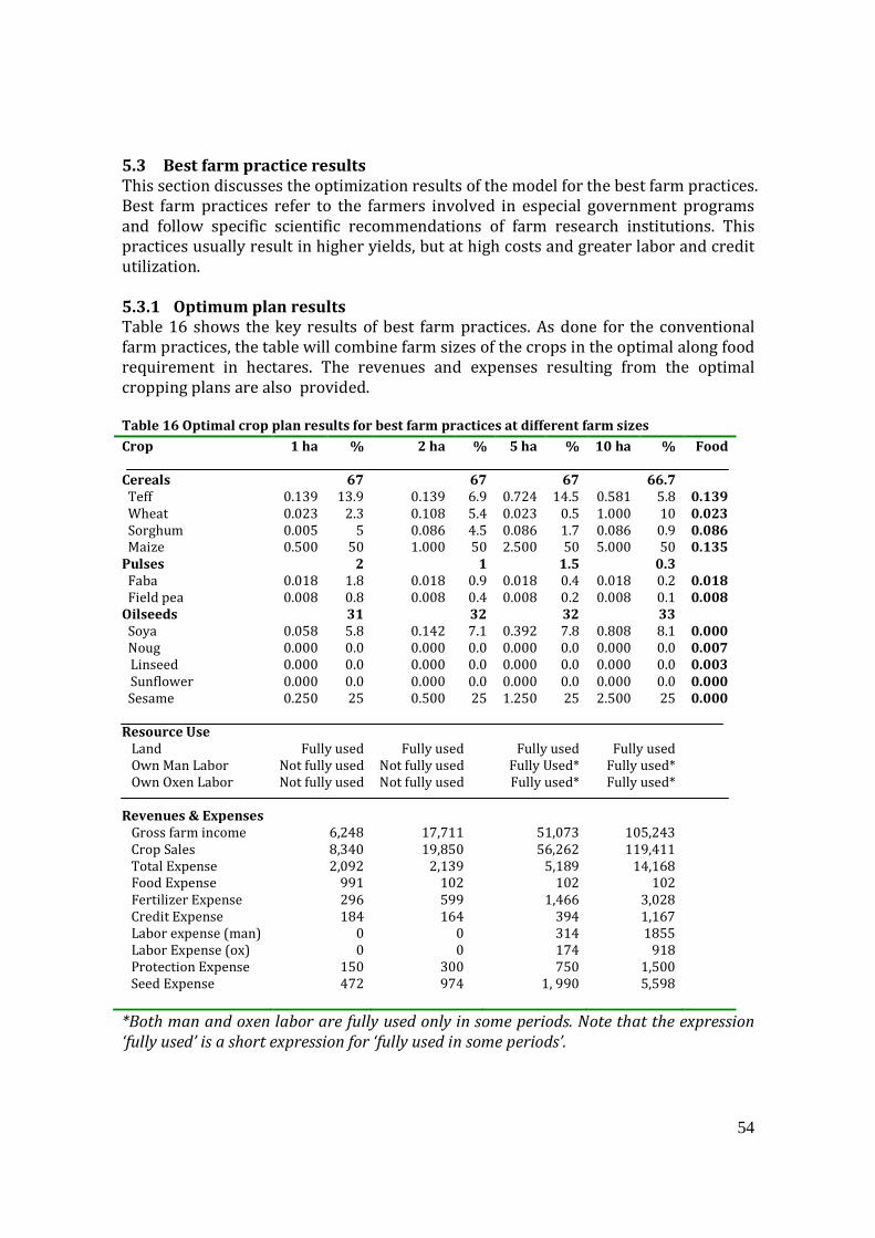
54
5.3 Best farm practice results
This section discusses the optimization results of the model for the best farm practices.
Best farm practices refer to the farmers involved in especial government programs
and follow specific scientific recommendations of farm research institutions. This
practices usually result in higher yields, but at high costs and greater labor and credit
utilization.
5.3.1 Optimum plan results
Table 16 shows the key results of best farm practices. As done for the conventional
farm practices, the table will combine farm sizes of the crops in the optimal along food
requirement in hectares. The revenues and expenses resulting from the optimal
cropping plans are also provided.
Table 16 Optimal crop plan results for best farm practices at different farm sizes
*Both man and oxen labor are fully used only in some periods. Note that the expression
‘fully used’ is a short expression for ‘fully used in some periods’.
Crop 1 ha % 2 ha % 5 ha % 10 ha % Food
Cereals
Teff
Wheat
Sorghum
Maize
Pulses
Faba
Field pea
Oilseeds
Soya
Noug
Linseed
Sunflower
Sesame
0.139
0.023
0.005
0.500
0.018
0.008
0.058
0.000
0.000
0.000
0.250
67
13.9
2.3
5
50
2
1.8
0.8
31
5.8
0.0
0.0
0.0
25
0.139
0.108
0.086
1.000
0.018
0.008
0.142
0.000
0.000
0.000
0.500
67
6.9
5.4
4.5
50
1
0.9
0.4
32
7.1
0.0
0.0
0.0
25
0.724
0.023
0.086
2.500
0.018
0.008
0.392
0.000
0.000
0.000
1.250
67
14.5
0.5
1.7
50
1.5
0.4
0.2
32
7.8
0.0
0.0
0.0
25
0.581
1.000
0.086
5.000
0.018
0.008
0.808
0.000
0.000
0.000
2.500
66.7
5.8
10
0.9
50
0.3
0.2
0.1
33
8.1
0.0
0.0
0.0
25
0.139
0.023
0.086
0.135
0.018
0.008
0.000
0.007
0.003
0.000
0.000
Resource Use
Land
Own Man Labor
Own Oxen Labor
Fully used
Not fully used
Not fully used
Fully used
Not fully used
Not fully used
Fully used
Fully Used*
Fully used*
Fully used
Fully used*
Fully used*
Revenues & Expenses
Gross farm income
Crop Sales
Total Expense
Food Expense
Fertilizer Expense
Credit Expense
Labor expense (man)
Labor Expense (ox)
Protection Expense
Seed Expense
6,248
8,340
2,092
991
296
184
0
0
150
472
17,711
19,850
2,139
102
599
164
0
0
300
974
51,073
56,262
5,189
102
1,466
394
314
174
750
1, 990
105,243
119,411
14,168
102
3,028
1,167
1855
918
1,500
5,598

55
Despite the optimum cropping plan distribution of conventional farm practices, the
optimal plans of best farm practices are more uniform for all farm sizes including 1
hectare. Maize takes up 50% of the land in all optimum cropping plans which wasn’t
the case for the conventional farm practices. The major reason for this is related with
the higher yields of best farm practices, usually double of the conventional practices.
Higher yields enable the best farm practice cropping plan to cover the minimum food
requirement with a much smaller farm sizes. For instance, farm sizes of 0.258(teff),
0.145(sorghum) and 0.043(faba) were required to meet the food demand of the
respective crops. But under the best practices, these figures were reduced to
0.139(teff), 0.086(sorghum) and 0.018(faba). This provides more land available for
sales and revenue generation of crops with high gross farm income. Pulses are grown
only to meet the food requirement with a crop size of 0.018 and 0.008 hectares, as
seen forr faba and field pea respectively.
Under cereals, teff and wheat are grown to meet the minimum food requirement in
the 1 and 2 hectare plans. But they are sold under 5 and 10 hectare cropping plan as
their respective land shares exceeded the minimum hectare needed to secure food
demand. On the whole, cereals have once again consumed the maximum allowed land
proportion, i.e., 67%. This shows cereals are still more attractive financially than the
other crop families. As expected, soya bean and sesame utilized most of the land left
from cereals. Sesame was grown at a maximum allowed land share. Soya beans utilize
the remaining land. This proves these two crops are the most profitable crops to grow
in rotating with cereals. Rotating as discussed above is necessary to avoid the
deterring effects of mono-cropping.
Assessing the resource usage influencing the cropping plan, land is once again a
common limiting factor throughout all plans. As it can be recalled, oxen labor becomes
a binding factor in some periods for farm sizes of 5, while human labor becomes
limiting only at 10 hectares under the conventional farm practices. However under
best farm practices, human labor becomes binding before oxen labor. This is noted
from the details of GAMS solution report where more human labor is hired than the
oxen labor. Credit was used in the crop plans of all farm sizes but not to the fullest
extent. But the amount of credit used under best farm practices is by far greater than
used under conventional practices. This is due to the high level of cash related
expenses under best farm practices. The cash expenses and the relation with credit
will be discussed in the upcoming paragraphs.
As far as revenue and expense figures are concerned, there is a new cost category
under the best farm practices, this is indicated as crop protection expense. This is the
cost of extra care required under best farm practices that are not prevalent under the
conventional farm practices. It is linearly related with the farm size like the fertilizer
cost. It increased from 150 to 300 birr as farm size rise from 1 hectare to 2 hectares.
Roughly, the same analysis can be made for the fertilizer cost. Gross farm income is
reasonably high even for 1 hectare. It was only about 600 birr under 1 hectare for the
conventional farm practice. This figure is as high as 6,248 birr in the best farm
practices. The major reason for this normally high gross farm income as indicated has

56
to do with the higher yields of best farm practices, usually double of the conventional
practices. This enables the best farm practices to cover the minimum food
requirement with a much smaller farm sizes. This provides the opportunity making
more land available for sales and revenue generation.
Food cost is still the highest cost incurred for the 1 hectare size and it is the only case
where the food cost exceeded the fertilizer cost. Beyond 2 hectares, the food cost
remained constant at 102 birr which is of course incurred for purchasing noug and
linseed since the minimum threshold of them are not met in the optimum crop plans.
Additional food purchase caused by sorghum is the reason behind the unusually high
food cost of the 1 hectare situation. There is no labor expense until 5 hectare is
reached. But it is important to note that contrary to the conventional farm practice
results, human labor costs (314 birr) were higher than oxen hiring costs (174 birr)
under the best practices. This is partly due to the extra human intervention and care
required to keep the crops in the best possible conditions.
Another important distinction between the conventional and best farm practice
results is the level of interest expense. Interest expenses are relatively much higher
for best practices. Interest expense is 184 birr under the 1 hectare cropping plan. This
means a credit of 1840 birr is used as the cost of borrowing was set at 10%. The credit
taken is only 160 birr from the maximum allowed credit, i.e., 2000 birr per hectare.
Clearly, interest expenses are more significant for the 1 hectare farm size. For instance,
the credit taken per hectare under the 1 hectare plan is 1, 840 birr while it is 820 birr
under 2 hectares and so on. However, in general, this points to the importance of
credit for the best farm practices because it involves high level of cash related
expenses. The unique cost that requires large amount of cash in fact was the seed
expense. Seed expense was uncharacteristically the highest expense of all the
expenses under best practices. This is expected since best seed varieties can only be
used and the seeds can only be bought from a special seed market at a remarkably
high price.
5.3.2 Sensitivity analysis
Sensitivity analysis was also done for the best farm practices. Changes made for the
conventional farm practices will be repeated with an extra analysis in this case. That
additional sensitivity analysis is made for discussing the effect of changing the level of
credit available. Credit has proven to be a big player in the best farm practices due to
higher cash expenses. The other variables to be discussed are the increase in price of
oilseeds, and decrease of labor force.
5.3.2.1 Increasing price of soya bean and sunflower
Table 17 below presents how the optimal cropping plan changes with the increase in
price of Soya beans and Sunflower under the best farm practices.

57
Table 17 Increasing price of soya bean (4.0) and sunflower (5.25) at a farm size of 5 hectares.
Crop Base Increase
by 0.5
Increase
by 1.00
Increase
by 1.5
Increase
by 2.0
Crops
Cereals
Teff
Wheat
Sorghum
Maize
Pulses
Faba
Field pea
Oilseds
Soya
Noug
Linseed
Sunflower
Sesame
Revenues and Expenses
Gross farm income
Crop Sales
Total Expense
Food Expense
Fertilizer Expense
Interest Expense
Labor Expense
labor Expense(man)
Labor Expense (ox)
Crop Protection Expense
Seed Expense
67%
0.724
0.023
0.086
2.500
0.5%
0.018
0.008
32.5%
0.392
0.000
0.000
0.000
1.250
51,073
56,262
5,189
102
1,466
394
488
314
174
750
1, 990
67%
0.329
0.419
0.086
2.500
0.5%
0.018
0.008
32.5%
1.225
0.000
0.000
0.000
0.417
51,877
57,936
6,059
105
1,321
481
444
291
153
750
2,959
66%
0.330
0.417
0.086
2.500
0.3%
0.000
0.008
32.7%
1.242
0.000
0.000
0.000
0.417
53,258
59,612
6,354
312
1,321
510
446
293
153
750
3,014
66%
0.330
0.417
0.086
2.500
0.3%
0.000
0.008
32.7%
1.242
0.000
0.000
0.000
0.417
54,646
61,103
6,457
312
1,321
521
446
293
153
750
3,108
66%
0.325
0.422
0.086
2.500
0%
0.000
0.000
33.3%
1.250
0.000
0.000
0.000
0.417
56,040
62,714
6,673
410
1,322
542
447
294
153
750
3,202
The response of soya and sesame to the price increases is almost similar to the
observation under the conventional farm practices. Soya bean is still more responsive
to the price increase than sunflower. The only difference under this plan is that a price
has to be increased by 2.00 for one of the crops(soya bean) to reach the maximum
allowed share of land. This is partly due to the relatively low crop share in the starting
point (0.392 hectares). Sunflower’s share in the optimal plan did not change despite
the price jumps. With every 0.5 birr increase in price of both the crops the gross farm
income showed a steady growth of 800 birr per hectare.

58
5.3.2.2 Credit
Credit is the main constraint with the biggest impact on the results of the optimal
crop plans. Table 18 presents the changes in the optimal plans resulting from
minimizing the allowed credit per hectare from 2000 birr to 250birr, 500 birr and
1000 birr. Ethiopian farmers constantly face lack of sufficient credit availability and it
is important to have a prism of lower credits.
Table 18 Changes in credit level at a (best practice) farm size of 5 hectares
Crop Base (Credit 2000) Credit 1000 Credit 500 Credit 250
Cereals
Teff
Wheat
Sorghum
Maize
Pulses
Faba
Field pea
Oilseeds
Soya
Noug
Linseed
Sunflower
Sesame
3.333
0.724
0.023
0.086
2.500
0.026
0.018
0.008
1.642
0.392
0.000
0.000
0.000
1.250
3.333
0.724
0.023
0.086
2.500
0.026
0.018
0.008
1.642
0.392
0.000
0.000
0.000
1.250
3.334
0.139
0.023
0.813
2.359
0.026
0.018
0.008
0.918
0.511
0.013
0.005
0.000
0.389
2.858
0.139
0.023
0.446
2.250
0.026
0.018
0.008
0.026
0.000
0.013
0.005
0.004
0.004
Resource Use
Credit
Land
Not fully used
Fully Used
Not fully used
Fully used
Fully used Not fully used
Fully used Not fully used
Labor
Gross farm income
Crop Sales
Total Expense
Food Expense
Fertilizer Expense
Interest Expense
Labor Expense
Labor Expense(man)
Labor Expense (ox)
Crop Protection Expense
Seed Expense
Fully used
51,073
56,262
5,189
102
1,466
394
488
314
174
750
1, 990
Fully used
51,073
56,262
5,189
102
1,466
394
488
314
174
750
1,990
Fully used
42,764
46,514
3,750
0
1,243
250
104
104
0
641
1,512
Not fully used
30,329
32,829
2,500
0
967
125
0
0
0
435
973
As it can be seen, low credit has an extremely adverse impact on both the resource
usage and gross farm income. The gross farm income retains its normal stature when
the credit is set at 1000 birr per hectare and above. But it decreased by more than
20,000 birr from setting the credit to 250 birr per hectare and decreased by just less
than 10,000 birr as a result of a 500 birr per hectare credit and working capital. Credit
didn’t prove to be of a great influence under the conventional farm practice. Relatively
low level of farm expenses in the conventional farm practice helped preserve the
stability of gross farm income with lower credit availabilities.

59
The major reason behind the sharp fall in the gross farm income is mainly related with
the amount of land used. Not all of the land available was used under the 250 and 500
birr per hectare credit. This adversely decreases the sales since lower land use means
lower crop yield available for consumption and sales. Under a credit of 250 birr per
hectare, only 3.824 hectares of the 5 hectares available was utilized. This is due to the
fact that a credit of 250 birr per hectare is too low to meet the cash expenses incurred
from operating on 5 hectares. Consequently, the maximum credit allowed was utilized.
An interest expense of 125 birr results from a 10% credit expense of 1250 birr (250
birr * 5 hectares). The same can be said about the 500 birr credit per hectare with an
interest expense of 250 birr.
5.3.2.3 Low labor supply
Table 19 presents how the optimal cropping plan and economic results change as a
result of having a lower labor supply and higher wage rate at the same time.
Table 19 Impact of low labor supply at farm size of 5 hectares
Crop Base 30% Less 50% less Food
Cereals
Teff
Wheat
Sorghum
Maize
Pulses
Faba beans
Field pea
Oilseeds
Soya
Noug
Linseed
Sunflower
Sesame
3.334
0.724
0.023
0.086
2.500
0.026
0.018
0.008
1.642
0.392
0.000
0.000
0.000
1.250
3.334
0.458
0.290
0.086
2.500
0.026
0.018
0.008
1.642
0.392
0.000
0.000
0.000
1.250
3.334
0.247
0.500
0.086
2.500
0.026
0.018
0.008
1.642
0.392
0.000
0.000
0.000
1.250
0.139
0.023
0.086
0.135
0.018
0.008
0.000
0.007
0.003
0.000
0.000
Resource Use
Own Man Labor
Own Oxen Labor
Fully used*
Fully used*
Fully used*
Fully used*
Fully used*
Fully used*
Gross farm income
Crop Sales
Total Expense
Food Expense
Fertilizer Expense
Interest Expense
Labor Expense
Labor Expense (man)
Labor Expense (ox)
Crop Protection Expense
Seed Expense
51,073
56,262
5,189
102
1,466
394
488
314
174
750
1, 990
49,546
56,849
7,303
102
1,494
605
1,906
1, 037
869
750
2,446
48,654
57,311
8,657
102
1,516
741
2,743
1782
1231
750
2,806
*Both man and oxen labor are fully used only in some periods. Note that the expression
‘fully used’ is a short expression for ‘fully used in some periods’.

60
The effect of adverse labor conditions is again not as worse as expected. The gross
farm income decreased by only 1,527 birr (2.7%) as a result of depressing the labor
by 30% and only by 2,419 birr (4.8 %) from cutting the labor by 50%. The increase is
mainly from an increase of labor expense. Throughout the labor force cuts, the labor
expense increased from 488 birr to 1,906 birr and to 2,743 birr with the labor cuts.
The cropping plan changed throughout the decrease in labor supply. There was a rise
in share of wheat from 0.023 ha to 0.290 ha and the land share of teff was downsized
from 0.724 hectares to 0.458 ha. As seen in Appendix 1 and 2, teff needs more man
and oxen labor than wheat in a period with the highest labor shortage and that is
period 7. In the model, period 7 represents the days ranging from June 20 to July 3 GC
which is a rainy season in Jimma. Farmers has to plant a lot of crops in this period to
gain advantage of the rain.
Despite what was observed under the conventional farming, the logical adjustment
due to the low labor supply holds under the best farm practices. The share of a crop
with lower labor requirement in period 7(wheat) increased while the share of a crop
with higher labor requirement (teff) decreased. This is because all the land shares of
the cereals under the base have already met the minimum food requirement. There
was no need to decrease a share of crops that are on the minimum level of hectares to
meet the food demand. As shown in table 19, teff, wheat, sorghum and maize need
0.139, 0.023, 0.086 and 0.135 hectares to meet the food demand which is already met
in the 5 hectare plan. Thus, the share of wheat can be increased without any
additional forms of cost, except labor cost. As a result, the share of teff decreased and
that of wheat increased.

61
6 Discussions, conclusions and recommendations
This final chapter broadens the discussion of preceding chapters to issues that are
related to major methodological choices and the overall implication of model results. In
section 6.1, major discussion points related to methodological issues are raised. In
section 6.2, some points derived from empirical results of this thesis are analyzed.
Section 6.3, general conclusions from this research are given. Section 6.4 presents
various recommendations and ideas for further research.
6.1 Methodological issues
A number of critical decisions and methodological choices were made during this
thesis. Developing a farm model especially for Ethiopia where there has been literally
no research on the subject is a challenge by itself and requires a number of decisions.
6.1.1 Model re-usability and representation
By definition, models are abstractions of reality and consequently they cannot include
all factors that influence a certain phenomenon. Some variables that may impact crop
production and overall efficiency were not included in the model for various reasons.
For instance, the profile of farmers in terms of their level of education, access to key
agricultural information and consultation can impact farmer effectiveness. This may
add another perspective to the model that can make it more comprehensive.
On the other hand, the model developed in this thesis is customized for the region of
Jimma. But it doesn’t represent a specific agronomic condition. The annual rainfall, the
soil type, the humidity and the altitude for which data was collected does not reflect a
particular agronomic and topographic conditions. The model was created for an
average rainfall, soil fertility, temperature and altitude in the region. This has both
advantages and disadvantages. On the advantage side, it has a broad appeal of
representing many regions in Ethiopia that have the topographic and agronomic
condition within the limits of Jimma region. But it can serve as a basic framework for
future models. Future researchers can exclude or include crops, change yields,
increase or decrease labor demand and other variables and can still follow the model
structure to a great extent.
6.1.2 Crop rotation scheme
Determining the share of the three crop families was a difficult task due to two reasons.
First, Ethiopian farmers are in general unfamiliar with oilseed crops and including
oilseeds in the cropping plan further complicated how land should be allocated. Secondly,
the major rotation practice in Ethiopia is rotating cereals with pulses and even
sometimes, cereals with cereals. It is easy to infer that cereals should consume a larger
part of the land, but how much to assign was only settled after consulting plant
researchers at PRI Wageningen University (Wijnands et al, 2011). With the oilseeds in
the picture as a new crop family to be introduced, the crop rotation scheme remains
ambiguous and more complex. That is why the thesis needed a crop rotation rule that
handles these three crop families in a well-structured scientific manner.

62
Conducting a field research and interviewing the farmers would have helped to adopt a
more representative and flexible crop rotation rules, but doing so would not result in a
fundamentally different rotation scheme crafted in the model. The model assigned a
maximum of 67% of the land to the cereals and the rest is left for either pulses or
oilseeds. Individual cereals can grow on a maximum share of 50% of the total land under
cultivation while individual pulses and oilseeds can claim up to 25% of the land. Even if
67% is a big share by any measure, surprisingly it is not sufficient when compared with
the reliance of Ethiopian farmers on cereals. As noted, farmers of Jimma region on
average grow cereals over 80% of their farm land.
The model delicately handled the three crop families in a way it is in parallel with the
actual farm practice and in a way the rotation sequence preserves soil fertility and
enhance crop yields. Hence, the actual farm practice, soil fertility and crop yields were
balanced while formulating the crop rotation rules adopted in the model. As a result, the
crop rotation rules of the model are not purely the same with the scientific
recommendations and yet they are not perfectly similar to the actual rotation practices
of farmers in Ethiopia. Table 20 below reviews model results by excluding oilseeds and
assigning all the land to either cereals or pulses to make it closer to the actual farm
practice.
Table 20 Results of other rotation rules at farm size of 5 hectares
Crop Base Rotation rule X* Rotation rule Y*
Cereals
Teff
Wheat
Sorghum
Maize
Pulses
Faba beans
Field pea
Oilseeds
Soya
Noug
Linseed
Sunflower
Sesame
3.334
0.258
0.431
0.145
2.500
0.061
0.043
0.018
1.606
0.656
0.000
0.000
0.000
0.950
5.000
0.295
2.000
0.145
2.500
0.000
0.000
0.000
0.000
0.000
0.000
0.000
0.000
0.000
5.000
0.258
0.067
0.145
4.531
0.000
0.000
0.000
0.000
0.000
0.000
0.000
0.000
0.000
Gross farm income
Crop Sales
Total Expense
Food Expense
Fertilizer Expense
Interest Expense
Labor Expense
Seed Expense
23, 457
24, 851
1,394
102
1,199
14
79
0
24, 587
27, 069
2482
376
1706
96
305
0
25,612
28,103
2491
376
1832
121
162
0
*Rotation rule X: Oilseed crops are excluded from the rotation while keeping rotation rules
limiting the maximum share of individual crops. But there is no limit on crop families
(cereals, pulses and oilseeds)

63
*Rotation rule Y: Oilseed crops are excluded from the rotation without any other rotation
rules
As it is shown avoiding oilseed crops from rotation since they are new crops to Ethiopian
farmers has a positive impact on gross farm income as it increased through those
transitions. But these spike in the gross farm income are not sustainable and are not as
positive as they seem. The biggest problem with these kind of rotations is their
detrimental effect of soil fertility and crop yield. Following the cropping plan indicated in
the last two columns may give a farmer such a high gross farm income on the first time
tilling or in the first season. But rotating within the same crop family and growing a
single crop (maize) over such a huge share of land will harm the soil and the crop yields
will continuously decline. Thus, the observed gross farm income cannot be kept at the
same level or increased.
6.1.3 Assumptions made in the thesis
There are substantial alternatives to some assumptions made in developing the model.
The major ones that deserve critiques are the ones made with regard to labor and land.
As far as labor goes, there was an assumption that kept the model simple and more
efficient. That is the constant wage rate assumed in hiring labor. For all farm activities ,
the cost of hiring was considered constant despite the fact that some farm functions
require slightly more skills than others. This, not only made the handling of labor simple,
but also avoided the arduous task of setting up a mechanism to trace which farm
activities are hired in which period and assigning a different wage rate to each activity.
Even if customizing the rate of hiring to different farm activities will make the model far
more complicated, it is sometimes that can potentially better the model. The main
concern in going through that road is the costs of setting up that mechanism may out
weight the benefits of performing it.
Despite this, however, the model adopted a very robust way of handling the labor supply.
The model deserves much credit for dissecting a single farming season in to 26 periods
on a 2 weeks basis and assign different levels of labor supply to each period depending
on labor mobility and seasonal migrations that affect the labor supply. The flexibility
enjoyed by this mechanism made it easy to account labor additions as a result of labor of
the students of the family available during school breaks. The only weakness in this
regard is the failure of the model in considering labor supply additions resulting from
labor migrations that are becoming prominent in Ethiopian agriculture. During farm
peak seasons harvesting, there is a considerable migration of labor from North Ethiopia
to South.
The migration occurs for two reasons. Firstly, the harvest season involves the hottest
three months in Ethiopia in general. But in the north, the temperature is quite extreme
and there is a tendency of labor force shift to pass the time in the south. So, this creates
more labor in southern areas like Jimma region. Secondly, harvest season is quite labor
demanding and beside that, some farmers want to avoid risk of crop catastrophes from
unexpected rains. Hence, there is an urgency to perform harvesting on time to avoid the
negative effects of a possible rainfall. This labor demand provides an opportunity for
64
young labor in the North, where the lands are not so fertile to grow crops, to move south
and earn some money.
But money is not the only vehicle through which these transactions are made between
the migrants and the farming labor. In fact, the more frequently practiced exchange is in
terms of sharing the crop yields collected at the end of the farming season. Farmers do so
to avoid cash expense since financial liquidity is one of the major bottlenecks constantly
faced in Ethiopia. There is no standard share on how the yield is shared, which was one
of the major reasons why labor migration effect was ignored by the model. Yield
exchanges usually take place through an oral dialogue between a migrant and a farmer,
thereby making it difficult to adjust the crop yields.
As far as land is concerned, the model assumed that each hectare of the land can be used
for growing crops. Fallows are allowed in the model, but they won’t have a role in the
results observed in the previous chapter, resulting from the process of optimization.
Farmers may flexibly preserve some part their land for grazing and even may rent out
some pieces of land to other farmers. The possibility of renting out is not particularly
considered. There is an extremely limited information on land renting to include it in the
model on the one hand. But on the other hand, including the possibility can potentially
influence the results extracted from the model.
6.2 General discussion of results
To test the validity of the model, the results of actual and optimal cropping plans were
compared. There is a considerable proximity in the financial outcomes of both plans.
Nevertheless, it doesn’t guarantee a good representative model. A net difference of more
than 600 birr was observed between the two plans, in which the optimal plan recorded a
higher gross farm income. This indicates the actual crop growing plan doesn’t represent
the best possible scheme to maximize the gross farm income.
Food requirement has proven to be the most critical item in shaping the optimal
cropping plans. It also shapes the crop rotation schemes indirectly. Cereals take a
significant role in Ethiopian food security. This creates a natural demand of growing
these crops more than other crop families. The demand in turn drives the price of the
cereals up giving them a considerable advantage of a higher chance of being included in
the optimal plan. Accordingly, in both the conventional and best farm practices, cereals
(teff, wheat, sorghum and maize) consumed most of the land allowed. In all farm sizes,
cereals did consume 67% of the land, which is the maximum allowed share of the land
for the crop family. Except for the 1 hectare plan under the conventional farm practice,
maize utilized nearly 50% of the land. Maize’s high yield, high gross margin and its
relatively lower labor consumption were the major reasons for its inclusion in the
optimal results. The prospect of maize is even brighter when the demand for the crop as
a food source and its new role as an energy source (ethanol) is considered.
Apart from the land share of cereals in the optimal cropping plan, the role of pulses(faba
and field peas) and oilseeds (soya, noug, linseed, sunflower and sesame) are more or less

65
the same under both the conventional and best farm practices. Pulses were mostly
grown over the minimum land required to meet the food demand. Soya bean and sesame
were the only two oilseed crops that managed to be in the optimal plan despite the fact
that noug and linseed were more critical for food security. Noug and linseed were
purchased from the external market to meet the food demand rather than growing them,
which was found to be preferable to maximize the gross farm income.
Hence, in general, at normal conditions of conventional and best farm practices, soya
beans and sesame are in the optimal cropping plan, but their significance comes second
to the cereals. Even if their share is marginal, their contribution in the optimal plan also
has a good prospect like maize. There are efforts by food security advocacy groups to
enable Ethiopian farmers to diversify their food sources. This is a good policy and also
beneficial to the farmers. These efforts can potentially divert the enormous dependence
on cereals for food to oilseeds. The extra demand created will cause a rise in price of
oilseeds. This will in turn make the gross farm income of oilseeds more attractive and
increases the level of their involvement in the optimum cropping plan.
A significant difference between the optimal results of conventional and best farm
practices is recognized when the effect of constraints is assessed through sensitivity
analysis. Under best farm practices, limiting credit facilities has proven to have a far
more negative impact. When the credit level is set at less than 1000 birr per hectare ,
there will be a fallow land in the 5 hectare and larger crop plans. Fallow lands (unutilized
pieces of farm land) significantly decrease crop sales from yields and ultimately causing
a sharp decline in the gross farm income. Land becomes not binding for the first time
throughout the analysis of model results when credit is fixed at low levels. In relation to
this, the cash need under the best farm practices was higher than the conventional farm
practices, which was why credit limitation had such a huge negative impact.
In assessing the prospect of oilseeds through price rises, the participation of soya
bean in the optimal cropping plan can be doubled with a slight increase of 0.5 birr/kg
in its price. The price of sunflower has to be increased by 3 birr to be included in the
optimal plan, which is a big ask. Even by then, its contribution is marginal.
The impact of labor was not as big as anticipated, which was demonstrated by the
marginal negative impact of unfavorable labor conditions on the gross farm income.
Under conventional farm practices, labor becomes binding only for 5 hectares and
larger farm sizes. And oxen labor becomes binding before human labor. But it is
human labor that becomes binding before an oxen labor under best farm practices.
The demand of human labor under best farm practices is higher than oxen labor due
to the extra human intervention needed to delicately handle the crops and vice versa
under the conventional farm practices.

66
6.3 Conclusions from results
The major conclusions from the thesis are:
1. The model developed in this thesis is a flexible and reasonably a sound
representative of the actual farm practice in the region. There are some
drawbacks, if dealt with would make the model more representative at the cost
of making it more complex. Nevertheless, considering the fact there were no
significant past works in farm modeling of Ethiopia, the model can be regarded
as a good start. The difference of 600 birr (around 11% above the actual plan)
between the income of the optimal and the actual cropping plan indicates that
the model is not that far away from the farm reality. On the other hand, the
model introduced relatively new crops (Oilseeds) to a typical farm and induced
greater competition within crops for limited resources. The new crops were fit
to the actual farm situation effectively so that food security and financial
demands of the farmers were met. But as a future recommendation, farm
research institutes in Ethiopia should actively take on farm modeling for better
understanding of crop production on Ethiopian farms.
2. The optimal crop plan of the model yielded a greater financial outcome than
the actual cropping plan adopted from the CSA data. The deciding factor in
gross farm income improvement from the optimal results was how the land
that is left over from cereal crops was utilized. In actual farm practice,
pulses(faba and field pea) and some oilseed crops(noug and linseed) were
grown along the cereals. These crops were not attractive financially and
instead of them, soya bean and sesame were included in the optimal plan.
These crops had a positive impact on the gross farm income. Hence, there is
room for improving farmers income and sustain crop yields at a desired level
through further research in farm modeling and better land distribution among
the crops.
3. Food requirement played a critical role in establishing a framework in how the
land is distributed in the optimal cropping plans. In general, crops that are an
important source of food security have higher prices, giving those crops an
edge to be included in the optimal results. Cereals, with a leading role of maize
(50% of the land mostly), took a great role in most of the cropping plans. Soya
beans and sunflower are the two oil seed crops that covered most of the land
left over from the cereals. Pulses were grown on the minimum land required to
meet the food demand.
4. Increasing the price of soya bean by a slight 0.5 birr/kg increases its share in
the cropping plan by a significant proportion, but the price of sunflower has to
rise monumentally to have a considerable role in the optimal results.
5. The optimal results of the conventional and best farm practices more or less
have the same nature. However visible differences arise when the role of the
constraints were assessed. Land was found to be binding in all cases except the
case of low credit facilities under the best farm practices. Low credits resulted
in unused land under best farm practices hugely impacting the gross farm

67
income. For that reason, credit providers (banks and the government) should
make sure that farmers under best farm practice preserve sufficient level
liquidity. Oxen labor is scarcer than human labor while human labor takes that
role under the best farm practices. Thus, conventional practice farmers should
put forward a continuous effort in rescheduling oxen labor and minimizing
oxen hiring as much as possible. The same implication can be made for the best
practice farmers with regard to the human labor
6.4 Recommendations for future researches
The research presented in this thesis leads to a number of new, interesting and
relevant research topics. There are also ways to improve the model in this thesis. The
model can be made more comprehensive by adding other factors that can possibly
influence the gross farm income and the decision making process of farmers. These
factors can be the effect of farm cooperatives, farmer’s level of education and access to
information. Many of the modeling decisions in this thesis were kept straight forward,
flexible and simple due to lack of past works and data limitations. The model can be
made more challenging and robust by setting up various mechanisms to further make
it more flexible. One of this adjustment can be expanding options of labor and creating
a set up through which variable rate of hiring is possible.
It has been indicated also that the model doesn’t represent a perfectly specific
agronomic and topographic condition since most of the general information about the
agricultural environment were based on an average basis. It is recommended for the
future a farm model be developed for a specific soil type, rainfall amount and weather
condition so that a more direct interpretation of model results for specific regions and
individual farmers can be made. Detailed regional or farm specific data bases can be
used for creating such models. Economic analysis such as marginal analysis of various
factors, credit-fertilizer correlation and other correlations can further enrich the
comprehensiveness of this research.
Formulating crop rotation rules was a difficult task in developing this model. To
improve model performance in this regard, farm observation and field research is
recommended for the future. Finally, GAMS software has been very helpful in
conducting this thesis. But other open source software like JAVA or R can be used for
optimization with a greater detail and complexity.

68
References (Literature and websites)
Abenet, B., Dillon, J. and Frank, M. (1992) Efficiency of small-scale farmers in Ethiopia:
A case study in the Baso and Warana sub-district. Elsevier Science Publishers
B.V., Amsterdam.
Abrar, S. (2003) Estimating Supply Response in the Presence of Technical Inefficiency
Using the Profit Function: An Application to Ethiopian Agriculture. Discussion
Papers in Economics #03/04. UK: University of Leicester. Accessed on: August
13, 2010
Addis A. (2003) Economic Development and Democracy in Ethiopia (Ph D thesis).
Erasmus University of Rotterdam. Rotterdam, The Netherlands.
Adenew, B. (2004) The food security Role of agriculture in Ethiopia. Ethiopian
economic policy research institute. Journal of agricultural and development
Economics. Addis Ababa, Ethiopia. Accessed December 2010. Available at:
http://scholar.google.nl/eap.gov.et
Barnard, S., and Nix, J. (1999) Farm Planning and Control (2nd ed). Interprint Limited,
New York, USA
Bazaraa, M., Jarvis, J., Sherali, H. (1990) Linear Programming and network flows. – 2nd
ed. John Wiley and Sons, New York. 684.p. Beck G.S. (1965). A theory of the
allocation of time. The Economic Journal 75:493-517
Bekele, S. and Stein, H. (1999) Soil Erosion and Smallholders’ Conservation Decisions
in the Highlands of Ethiopia, Agricultural University of Norway, As, Norway.
Bekele, S., and Stein H. (1999) Soil Erosion and Smallholders’ Conservation Decisions
in the Highlands of Ethiopia. Agricultural University of Norway.
Berhanu, N. and Samuel, G. (2002) Land Tenure and Agricultural Development in
Ethiopia, Addis Ababa: Ethiopian Economic Association.
Bulcha, W. (2007) Guizotia abyssinica. In: VOSSEN, H. A. M. V. D. & MKAMILO, G. S.
(eds.) PROTA (Plant Resources of Tropical Africa / Ressources végétales de
l’Afrique tropicale).
Campell, R. and McConnel, S. (1999) Economics: Principles, Problems and Policies,
14th ed. Boston: McGraw-Hill.
Carswell, G., Data, D., De Haan, A., Alemayehu, K., Haileyesus, S. and Sinclair, A. (2000).
Ethiopia Country Report. IDS Research Report, Brighton, IDS.

69
Castano, J.(2001) Agricultural Marketing Systems and Sustainability: Study of Small
Scale Andean hillside farms, PhD thesis, Wageningen University, Wageningen,
The Netherlands.
CIA. (2010). The World Factbook: Ethiopia [Online]. USA Central Intelligence Agency.
Available: https://www.cia.gov/library/publications/the-world-
factbook/geos/et.html [Accessed September 2010].
Claassen G., Hendriks, Th. and Hendrix, E. (2007) Decision Science: Theory and
Applications. Wageningen, Wageningen Academic Publishers, Mansholt
Publication Series, Vol. 2.
CSA (2005) Population Statistics 2004/2005, Central Statistical Agency of Ethiopia
CSA (2009a) Agricultural Sample Survey 2008/2009. Area and production of crops.
Addis Ababa: Central Statistical Agency of Ethiopia.
CSA (2009b) Report on crop and livestock product utilization in 2008/2009. Addis
Ababa: Central Statistical Agency.
CSA (2009c) Report on farm management practices. Addis Ababa: Central Statistical
Agency.
Demeke, M. (1999) Ethiopian Agriculture since 1991: Its Performance and Challenges
Faced, presented to the Symposium for Reviewing Ethiopia’s Socioeconomic
Performance 1991-1999.
EEA (2002) Second Annual Report on the Ethiopian Economy. Addis Abeba, Ethiopia.
EIAR (2010). Company profile, Ethiopian Institute of Agricultural Research. Available
at http://www.eiar.gov.et/about-eiar. Accessed on August 2010.
FDRE. (2000). The Second Five-year Agricultural Development Program, 2000/01-
2004/05, November 2000 (in Amharic).
Fistum, H., Goswill, M., Regass, E., and Seleshi, B.(2006): Importance of Irrigated
Agriculture to the Ethiopian Economy, International Water Management
Institute Research Report 128, Addis Ababa, Ethiopia.
Gabre-Madhin, E. (2001) Market Institutions, Transaction Costs, and Social Capital in
the Ethiopian Grain Market, IFPRI Research Report, No.124, Washington DC:
International Food Policy Research Institute
Gabre-Madhin, E. and Goggin, I. (2006) Does Ethiopia Need a Commodity Exchange?
An Integrated Approach to Market Development, EDRI-ESSP Policy Working
Paper, No.4, Addis Ababa: Ethiopian Development Research Institute.

70
Gasson, R. (1973) Goals and Values of Farmers, Journal of Agricultural Economics,
Cambridge University, Cambridge, the UK.
Gelalcha, S. D. (2009) Sesame trade arrangements, costs and risks in Ethiopia: A
baseline survey. VC4PPD Report. Wageningen: Wageningen University and
Research.
Glen, J. (1986) Mathematical Models in Farm Planning. University of Edinburg.
Edinburg, Scotland.
Government of Ethiopia (2003) ‘The New Coalition for Food Security in Ethiopia: Food
Security Programme, Vol.1’, Addis Ababa: Ministry of Agriculture and Rural
Development
Kruseman, G. (2000) Bio-economic household modelling for agricultural
intensification. Ph. D. thesis. Mansholt Graduate School, Wageningen University,
The Netherlands. 256 pp.
MEDaC. (1999) Poverty Situation in Ethiopia. Welfare Monitoring Unit. Addis Ababa
MEDaC. (1999) Survey of the Ethiopian Economy, Review of Post-Reform
Developments, September 1999.
MOFED (2010) The Federal Democratic Republic of Ethiopia Growth and
Transformation Plan (GTP) 2010/11-2014/15 (Draft). Addis Ababa, Ministry
of Finance and Economic Development.
Reid, R., Kruska, R., Muthui, N. (2000) Landuse and landcover dynamics in response
to changes in climatic ,biological and socio2political forces:the case of
southwestern Ethiopia. L an dscape Ecol ,15 (4) :339-355
Romero, C., Rehman, T. (1984) Goal Programming and Multiple Criteria Decision
Making in Farm Planning: Expository Analysis, Universidad de Cordoba and
University of Reading, Earley Gate, Reading RG6 2AT, the UK.
Ross, H(2003) Soil PH and Plant Nutrients.
Samuel, G. (2006a) Land, Land Policy and Smallholder Agriculture in Ethiopia. Policy
Paper Prepared for the Future Agricultures Consortium and Presented at
Institute Development Studies, University of Sussex, March 22-22, 2006.
Samuel, G. (2006b) Population, Environment and Agricultural Development in
Ethiopia: Could The Dismal Prediction of Malthus Explain the Reality in
Ethiopia? Policy Paper Prepared for the Future Agricultures Consortium.

71
Samuel, G. (2006) Intensification of Smallholder agriculture in Ethiopia: Options and
scenarios, 2006 Available at: http://www.dfid.gov.uk/R4D//PDF, last accessed
September 14, 2010.
Schweigman, C. (2005) Operations Research Problems in Agriculture in Developing
Countries, Khartoum Universtiy Press, Khartoum, Sudan.
Shepherd, J. (1975) The Politics of Starvation. New York: Carnegie Endowment for
Inter-national Peace
Singh, H. (1987) Agricultural problems in Ethiopia. Gian Publishing House 29/6 Shakti
Nagar, Delhi, India. Available at: http://books.google.nl/books, Accessed on
August 2010.
Suleiman, A., Oliver, M. and Tony, R. (2004) Aggregate Agricultural Supply Response
in Ethiopia; A farm-level Anaylsis, University of Sheffield, UK
Tanner, D., Zewdu, Y., Lemma, Z. and Girmay, H. (1994) Potential for Cereal-Based
Double cropping in Bale region of Southeastern Ethiopia. African Crop Science
Journal, Nirobi, Kenya.
Thomas, R., Christopher, B., Julio A. and Johan F. (2009) Agrifood Industry
Transformation and Small Farmers in Developing Countries; Michigan State
University, USA
Tesfaye, Z. (2007) Technologies, Markets and Poverty: Evidence from Studies of
Agricultural Commodities in Ethiopia.; Socio-economics research program, p.1
UNHCR, (2010)The Right to Adequate Food. Fact Sheet 34. United Nations, New York,
USDA, (2010) USDA National Nutrient Database for Standard Reference [Online].
Washington: Agricultural Research Service,
Wijnands, J., Napol, G., Lute, J. and van Loo, E. (2011). Ethiopian soya bean and
sunflower value chains: Oppurtunities and Challenges, LEI, Wageningen
University, The Netherlands.
Wijnands, J.H.M., J. Biersteker and E.N. van Loo, Oilseeds business oppurtunities in
Ethiopia. LEI, part of Wageningen UR, The Hague, 2009.
World Bank (2006). Annual Review: Ethiopia. Available at http://web.worldbank.org/
Acceccessed, November 2010.
Yao, S. (1996). The Determinant of Crop Productivity of the Peasant Farm Sector in
Ethiopia; Journal of international Development: Vol. 8, No. 1, 69-82 (1996)
Department of Economics, University of Portsmouth.

72
Appendices:
Appendix 1:Man labor hours
General activity man hours- conventional farming and best farm practices General Activity Crops
Time Teff Wheat Sorghum maize fava fieldp Soybean neug linseed sunflower Sesame
Land
Preparation Period 1 12 12 12 12
Period 2 12 12
Period 3 12 12 12 12 12
Period 4
Period 5
Period 6
Period 7
Period 8
Period 9
Period 10
Period 1 1
Period 12
Period 13
Transport
and Storage Period 14
Period 15 24
Period 16
Period 17 16 8
Period 18 8 28 8 8 4
Period 19 8 24 24 16 4 4 8 16
Period 20 16 4 16
Period 21 16
Period 22 16
Manure
Application Period 23 4 4 4 4 4 4 4 4 4 4 4
Period 24 4 4 4 4 4 4 4 4 4 4 4
Period 25 4 4 4 4 4 4 4 4 4 4 4
Period 26 4 4 4 4 4 4 4 4 4 4 4

73
Man hours for tilling under conventional farming Tillage by ox Crops
Time Teff Wheat Sorghum maize fava fieldp Soybean neug linseed sunflower Sesame
Period 1 32
Period 2 32
Period 3 32 32 32
Period 4 16 32 32 32
Period 5 32 32 32 32 32 32
Period 6 64 48 16 32 32
Period 7 80 32 16 16 16 48 48 32
Period 8 32 16 16 16 16
Period 9
Period 10
Period 1 1
Period 12
Period 13
Period 14
Period 15
Period 16
Period 17
Period 18
Period 19
Period 20
Period 21
Period 22
Period 23
Period 24
Period 25
Period 26

74
Man hours for tilling under best farm practices
Tillage by ox Crops
Time Teff Wheat Sorghum maize fava fieldp Soybean neug linseed sunflower Sesame
Period 1 32
Period 2 32
Period 3 32 32 32
Period 4 32 32 32 32
Period 5 32 32 32 32 32 32
Period 6 64 48 32 32 32
Period 7 80 64 32 32 32 48 48 32
Period 8 64 32 32 32 32
Period 9
Period 10
Period 1 1
Period 12
Period 13
Period 14
Period 15
Period 16
Period 17
Period 18
Period 19
Period 20
Period 21
Period 22
Period 23
Period 24
Period 25
Period 26

75
Man hours for Sowing-Weeding under conventional farming
Sowing-weeding Crops
Time Teff Wheat Sorghum maize fava fieldp Soybean neug linseed sunflower Sesame
Period 1
Period 2
Period 3
Sowing Period 4 24
Period 5
Period 6 16 24
Period 7 40 24 16 16 32 40 16
Weeding Period 8 32 16
Period 9 48 32 32 32
Period 10 32 48 32 48 8
Period 1 1 32 36 32 32 32
Period 12 16 48 16 48 24 32
Period 13 48 16
Period 14
Period 15
Period 16
Period 17
Period 18
Period 19
Period 20
Period 21
Period 22
Period 23
Period 24
Period 25
Period 26

76
Man hours for Sowing-Weeding under best farm practices
Sowing-weeding Crops
Time Teff Wheat Sorghum maize fava fieldp Soybean neug linseed sunflower Sesame
Sowing Period 1
Period 2
Period 3
Period 4 48
Period 5
Period 6 32 48
Period 7 48 48 32 32 48 64 32
Weeding Period 8 32 32
Period 9 48 32 32 32
Period 10 32 48 32 48 8
Period 1 1 16 20 16 32 16
Period 12 8 16 8 8
Period 13 24 8
Period 14
Period 15
Period 16
Period 17
Period 18
Period 19
Period 20
Period 21
Period 22
Period 23
Period 24
Period 25
Period 26

77
Man hours for activities from harvesting, threshing and cleaning under
conventional farming
(Each crop has two labor figures under this activities. The first one corresponds to
harvesting. The second one relates to both threshing and cleaning)
Harvest, threshing
cleaning Crops
Time Teff Wheat Sorghum maize fava fieldp Soybean neug linseed sunflower Sesame
Period 1
Period 2
Period 3
Period 4
Period 5
Period 6
Period 7
Period 8
Period 9
Period 10
Period 1 1
Period 12
Period 13
Period 14 64
Period 15 128 24 96 96
Period 16 160 96 112
Period 17 48 104 112 96
Period 18 48 40 48 24 8
Period 19 104
Period 20 48 40 30
Period 21
Period 22 40
Period 23
Period 24
Period 25
Period 26
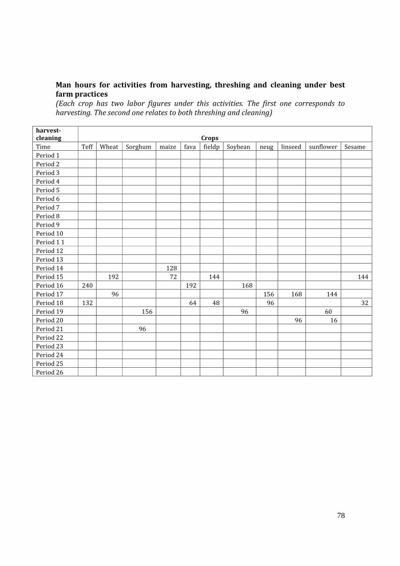
78
Man hours for activities from harvesting, threshing and cleaning under best
farm practices
(Each crop has two labor figures under this activities. The first one corresponds to
harvesting. The second one relates to both threshing and cleaning)
harvest-
cleaning Crops
Time Teff Wheat Sorghum maize fava fieldp Soybean neug linseed sunflower Sesame
Period 1
Period 2
Period 3
Period 4
Period 5
Period 6
Period 7
Period 8
Period 9
Period 10
Period 1 1
Period 12
Period 13
Period 14 128
Period 15 192 72 144 144
Period 16 240 192 168
Period 17 96 156 168 144
Period 18 132 64 48 96 32
Period 19 156 96 60
Period 20 96 16
Period 21 96
Period 22
Period 23
Period 24
Period 25
Period 26
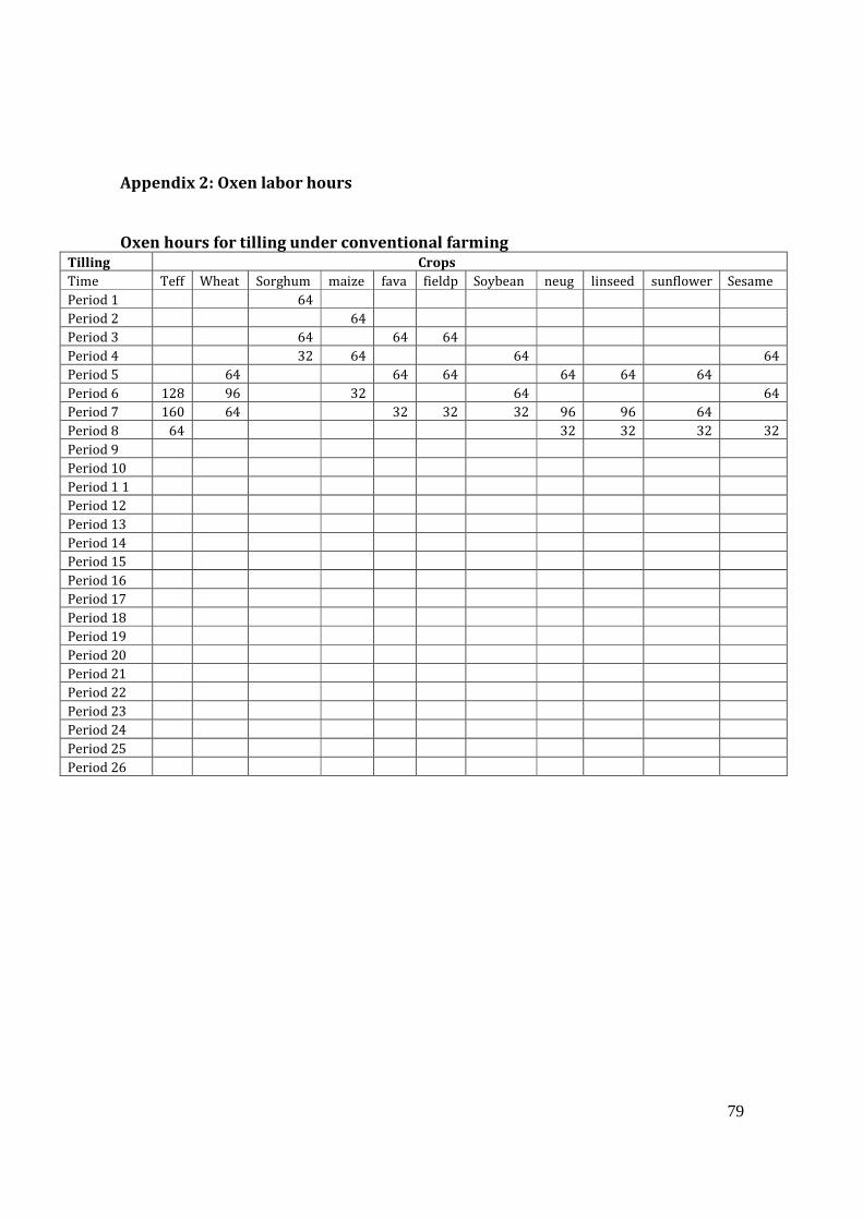
79
Appendix 2: Oxen labor hours
Oxen hours for tilling under conventional farming Tilling Crops
Time Teff Wheat Sorghum maize fava fieldp Soybean neug linseed sunflower Sesame
Period 1 64
Period 2 64
Period 3 64 64 64
Period 4 32 64 64 64
Period 5 64 64 64 64 64 64
Period 6 128 96 32 64 64
Period 7 160 64 32 32 32 96 96 64
Period 8 64 32 32 32 32
Period 9
Period 10
Period 1 1
Period 12
Period 13
Period 14
Period 15
Period 16
Period 17
Period 18
Period 19
Period 20
Period 21
Period 22
Period 23
Period 24
Period 25
Period 26
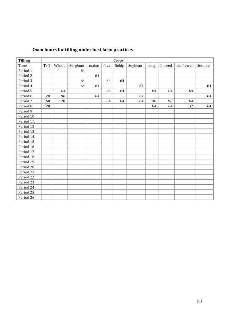
80
Oxen hours for tilling under best farm practices
Tilling Crops
Time Teff Wheat Sorghum maize fava fieldp Soybean neug linseed sunflower Sesame
Period 1 64
Period 2 64
Period 3 64 64 64
Period 4 64 64 64 64
Period 5 64 64 64 64 64 64
Period 6 128 96 64 64 64
Period 7 160 128 64 64 64 96 96 64
Period 8 128 64 64 32 64
Period 9
Period 10
Period 1 1
Period 12
Period 13
Period 14
Period 15
Period 16
Period 17
Period 18
Period 19
Period 20
Period 21
Period 22
Period 23
Period 24
Period 25
Period 26

81
Oxen hours for threshing under conventional farming
harvest
cleaning Crops
Time Teff Wheat Sorghum maize fava fieldp Soybean neug linseed sunflower Sesame
Period 1
Period 2
Period 3
Period 4
Period 5
Period 6
Period 7
Period 8
Period 9
Period 10
Period 1 1
Period 12
Period 13
Period 14
Period 15
Period 16
Period 17 96
Period 18 96 48
Period 19
Period 20 32
Period 21 40
Period 22
Period 23
Period 24
Period 25
Period 26

82
Oxen hours for threshing under best farm practices
harvest
cleaning Crops
Time Teff Wheat Sorghum maize fava fieldp Soybean neug linseed sunflower Sesame
Period 1
Period 2
Period 3
Period 4
Period 5
Period 6
Period 7
Period 8
Period 9
Period 10
Period 1 1
Period 12
Period 13
Period 14
Period 15
Period 16
Period 17 192
Period 18 192 96
Period 19
Period 20 64
Period 21 192
Period 22
Period 23
Period 24
Period 25
Period 26

83
Appendix 3: Production and utilization
Crop Production and consumption in Ethiopia and Jimma
Region Crop Production Consumption Seed Sale Wages Feed Other
Ton % % % % % % %
Ethiopia Cereals 144,964,059 66 16 14 1.3 0.6 3.0
Pulses 19,646,301 61 21 15 0.8 0.3 1.9
Oilseeds 6,556,044 53 12 29 1.3 0.1 4.6
Neug 1,906,523 24 13 60 1.3 0.1 1.2
Linseed 1,560,693 46 15 35 0.6 0.1 1.4
Sesame 2,166,406 19 10 68 2.4 0.1 0.6
Rapeseed 386,636 43 11 44 0.3 0.1 0.8
Jimma Cereals 6,299,960 60 13 11 3.3 0.3 2.6
Pulses 386,698 69 13 16 1.1 0.0 0.9
Oilseeds 89,196 53 12 29 1.3 0.1 4.6
Neug 50,632 32 15 51 0.1 0.9
Linseed 19,669 65 13 18 2.8 0.9
Sesame 12,066 40 4 55 0.5
Rapeseed 1,348 65 9 25 0.5 0.3
Appendix 4: Fertilizer and seed input
Fertilizer (individual nutrient required per hectare to facilitate crop growth)
Source: Prota database and USDA (2010)
Conventional farming Best farm practices
N P K N P K
Unit
Crops kg kg kg kg kg kg
teff 21.3 4.3 4.3 38.3 7.7 7.7
wheat 21.9 3.5 4.1 56.9 9.1 10.7
maize 15.0 2.1 3.2 60.2 8.4 12.8
sorghum 18.0 2.9 3.5 45.0 7.3 8.8
faba 42.0 4.2 10.6 105.0 10.5 26.5
fieldpea 36.0 4.6 10.4 74.0 9.2 20.8
soya 58.0 6.1 18.0 139.2 17.0 43.1
noug 29.0 6.0 6.0 23.2 5.6 5.6
linseed 31.2 5.0 8.1 28.1 4.5 7.3
sunflower 31.6 6.3 6.1 44.3 8.8 8.6
sesame 28.4 6.0 4.4 45.4 9.6 7.1

84
Seed amount required
Appendix 5: Crop rotation table
Crop coefficients of the crop rotation rules Constraint C1 C2 C3 C4 C5 C6 C7 C8 C9 C10 C11 Fallow RHS
land 1 1 1 1 1 1 1 1 1 1 1 <= Rb
CR1 2 0 0 0 0 0 0 0 0 0 0 0 </>= Rb
CR2 0 2 0 0 0 0 0 0 0 0 0 0 </>= Rb
CR3 0 0 2 0 0 0 0 0 0 0 0 0 </>= Rb
CR4 0 0 0 2 0 0 0 0 0 0 0 0 </>= Rb
CR5 1 1 1 1 -2 -2 -2 -2 -2 -2 -2 -2 </>= Rb
CR6 1.5 1.5 1.5 1.5 0 0 0 0 0 0 0 0 </>= Rb
CR7 0 0 0 0 4 4 4 0 0 0 0 0 </>= Rb
CR8 0 0 0 0 0 0 0 4 0 4 0 0 </>= Rb
CR9 0 0 0 0 0 0 0 0 2 0 0 0 </>= Rb
CR10 -1 -1 -1 -1 0 0 0 0 -1 3 0 -1 </>= Rb
CR11 -1 -1 -1 -1 -1 -1 -1 3 -1 0 0 -1 </>= Rb
CR12 0 0 0 0 0 0 0 4 4 0 0 </>= Rb
CR13 0 0 0 0 0 0 0 0 0 0 4 0 </>= Rb
Note:
C1-C11 represents the crops
Rb=Available farm size in hectares
Conventional
farming
Best farm
practices
unit Kg/hectare Kg/hectare
Crops Seed rate Seed rate
teff 30 30
wheat 150 150
maize 30 30
sorghum 15 15
faba 185 185
fieldpea 125 125
soya 50 50
noug 15 15
linseed 35 35
sunflower 15 15
sesame 15 15

85
Appendix 6: Costs (Inputs, hiring and food) in ETB
Activity
unit
Costs
Hiring man labor 1 hour 1.25
Hiring oxen labor 1 hour 0.75
Tilling by tractor 1 ha 500
Seedbed preparation by tractor 1 ha 250
Sowing by tractor 1 ha 500
Weeding by tractor 1 ha 75
Harvest, threshing and cleaning by
combine harvester
1 ha 1700
Urea 1 Kg 2.50
DAP 1 Kg 2.55
Interest on credit 1 ETB 0.1