fairness spillovers the case of taxation
TRANSCRIPT

Fairness Spillovers
–
the case of taxation
Thomas Cornelissena
University College LondonOliver Himmlerb
Goettingen University
Tobias Koenigc
Hannover University
first draft: October 2009this version: March 30, 2010
Abstract
It is standardly assumed that perceived injustice triggers behavioral adjustmentsin precisely the same area where the violation of justice has occurred. However,grievances over being exposed to injustice may have even broader consequencesand also spill over to other spheres, causing adjustments there. The behavioralconsequences of tax fairness perceptions indicate the presence of such a mechanism.Specifically, we show that the lower levels of tax morale which have been reportedin the literature need not be the only adjustment to violations of tax fairness. Inour estimations, a belief that the rich don’t contribute adequately to the tax base isalso associated with lower work morale. These “fairness spillovers” are surprisinglystrong, thus incurring large economic costs which have been neglected so far: Thebelief that the rich pay too little in taxes is associated with 20% higher levels ofpaid absenteeism due to illness.
Keywords: Tax Fairness, Taxation, Conditional Compliance, Reciprocity, SocialComparisonsJEL: J22, D63, H31, A13.
aUniversity College London, Department of Economics, Drayton House, 30 Gordon Street, London WC1H0AX, United Kingdom. email: [email protected]
bGoettingen University, Department of Economics, Platz der Goettinger Sieben 3, D-37073, Goettingen,Germany. email: [email protected]
cHannover University, Department of Economics, Koenigsworther Platz 1, D-30167, Hannover, Germany.email: [email protected]
We thank Christian Dustmann, Uta Schoenberg, Robert Schwager, Andreas Wagener and the partic-ipants of the CReAM seminar at UCL for helpful comments. An earlier version of this manuscripthas been circulated under the title ’Tax Fairness Perceptions and Economic Behavior – Evidence fromAbsenteeism’.

1 Introduction
People care about justice in taxation. Especially when it comes to the question of how
much to tax the rich. Consequently, this is one of the most widely discussed topics in
present-day politics and virtually every political actor has something to say about tax-
reform proposals for the upper income brackets. Fueled by the current financial crisis, a
soak the rich attitude is prevalent in many countries and tax increases for high incomes
are being discussed around the globe. Tax breaks for the rich on the other hand usually
don’t go down well with the public and are often accompanied by political protests. When
people are asked in opinion polls, questions about tax cuts for this part of the population
let emotions run high. In a recent Economist poll on US public opinion, people were
asked how angry they get when they think about “Tax Breaks for the Rich”. Almost half
of the respondents answered “Very Angry”, about one fifth get “Somewhat Angry” while
only one out of ten said they “Don’t think about it”.1 While the belief that the rich pay
too little in taxes, it is open to question whether these complaints translate into behavior.
This is what we empirically investigate in this paper.
The idea that people show behavioral responses to social environments perceived to be
unfair is widely held in the literature.2 Individuals condition their own contribution to
common goals on whether others contribute, i.e. whether others show co-operative or pro-
social behavior.3 Consequently, a lower willingness to comply with generally accepted
ethical codes results from the fact or belief that others violate social norms. A small
strand of research has applied these ideas to fairness in taxation. They ask whether a tax
system which is perceived to be unfair evokes compensatory actions in the form of tax
evasion.4 Carried over to our framework, feelings of unfairness may stem from the belief
that the rich do not contribute adequately to the tax pool – e.g. by taking advantage of
loopholes or by flat out evading taxes in an illegal manner. However, the blame need not
be on the rich themselves: agents may just as well feel that politicians fail to implement
tax policies that sufficiently strain the rich and thus deem the tax system unfair. As a
result of both mechanisms, the agents may decide not to comply with the norm to pay
their tax dues and attempt to restore equity by evading taxes. While at first glance tax
evasion is a plausible reaction to perceived injustice in taxation, it is not a viable option
for most. Taxable income is often directly reported to the government by employers
or other third-party institutions such as banks, investment funds, and pensions funds.
1Economist/YouGov Poll, conducted March 22-24, 2009.2For a survey of the fairness literature in economics, see Fehr and Schmidt (2005).3Frey and Meier (2004); Traxler and Winter (2009).4Andreoni et al. 1998, Feld and Frey 2002, McCaffery and Slemrod 2004 consider the role of tax fairnessand other cultural aspects for tax compliance.
1

This precludes the manipulation of tax returns (Kleven et al., 2010). However, this lack
of direct adjustment measures may create spillovers to other spheres of life: instead of
evading taxes, agents may resort to non-compliant behavior in surrogate areas. We argue
that the realm of the workplace is especially prone to such spillovers. The reason is that
exertion of effort at work is not fully contractible and therefore entails various elements
of “quasi-voluntary” contributions. Individuals who feel that the rich don’t pay their fair
share in taxes, suspect the rich of violating a norm by failing to contribute to the common
good, may reciprocate this norm violation by cutting back work effort, thus choosing not
to contribute to the common good by means of violating the norm of working hard, either.
That fairness spillovers may indeed exist can be inferred from situations where agents
utter that they refuse to make any effort above and beyond the call of duty at work
as long as those in charge do not contribute their fair share. This is obviously only
anecdotal evidence for the existence of the hypothesized spillovers and a rigorous way
of testing for their existence is more difficult to come up with, because such individual
’work-to-rule’ strategies are notoriously hard to observe and measure. We suggest a setup
where the sickness leave of German employees serves as a work morale measure that is
easy to observe, and that at the same time allows us to put a price tag on the fairness
spillovers and assess their economic relevance. In Germany, there is no reduction of
earnings associated with sickness spells of up to six weeks’ duration and, for the first
three days of each period of leave, employees are usually not even obliged to provide a
doctor’s note. In addition, there are high levels of job protection. We assume that this
legal generosity provides incentives to utilize it as as a means of shirking one’s duty when
others are suspected of not contributing to common goals, either.5 The data on sick leave
stems from the German Socio-Economic Panel (GSOEP), which in its 2005 wave also
includes questions about how people evaluate the fairness of the tax system at the upper
end of the income distribution. We take the belief that managers don’t pay enough taxes
to represent perceived unfairness in favor of the rich and use this variable to explain the
number of days absent from work, carefully conditioning on health status, a rich set of
income, personal and job related variables. We find that the belief that managers pay
too little in taxes is strongly negatively correlated with our indicator of non-compliant
behavior, even after netting out the factors mentioned above. The effect is robust to the
use of a variety of estimation methods and specifications. On average, employees with the
perception that managers pay too little in taxes accrue 20 percent more sick days, which
translates to 1.5 more days absent from work per year.
5This is not to say that everyone on sick leave is a shirker. However, that absence due to illness is notpurely a response to medical conditions is widely accepted in the labor economics literature (Barmby etal., 2002; Johannsen and Palme, 2005; Puhani and Sonderhof, 2010).
2
Our study is the first that empirically relates tax fairness perceptions to work effort, to
the best of our knowledge. It is closely related to literature in workplace psychology
– which largely builds on Adams’ equity theory (1963, 1965) – as well as work effort
experiments in economics (Fehr and Falk, 2002; Fehr and Schmidt, 2005). Both these
strands of literature analyze whether perceptions of fairness within the workplace matter
for work performance and define fairness in terms of reciprocity or conditional compliance.
They argue that when others take actions that violate certain work related norms – in
the case of equity theory the norm that the ratio of work input to work output should
be equalized, in the context of experimental economics the norm to give “kind” wage
offers – individuals adjust their own work effort in order to reciprocate. Departing from
direct reciprocity, we suggest work performance to be sensitive to compliance behavior
outside the realm of workplace. Hence, we raise the issue of indirect reciprocity or indirect
compliance: Individuals exhibit substantial adjustment behavior even in ways and areas
that at first seem far removed from the domain where the perceived injustice occurred.6
This is what we label ’fairness spillovers’.
This paper also contributes to the question of how taxation affects the economy. The
conventional wisdom is that taxation changes monetary incentives, e.g. by reducing the
opportunity costs of leisure, or the expected value of consumption. We suggest a comple-
mentary channel: People seem to have beliefs about fairness in taxation – and it is these
beliefs that provide an incentive on their own. Considering that the effects of perceived
unfairness on absenteeism are large, the costs of taxation could be quite different from
what is usually assumed. Put differently, a “hidden” excess burden of taxation may result
from the association between tax fairness and work morale.
The remainder of the paper is organized as follows. Section 2 provides a more detailed
exposition of how fairness perceptions may affect work morale. It also describes the
data and gives some descriptive statistics. Section 3 presents and discusses the baseline
empirical results. Section 4 presents robustness checks, and section 5 concludes.
2 Background, data and descriptive statistics
How do individuals react when their sense of tax fairness is violated? Fortunately, most
people will not go to such extremes as the person who decided to crash his airplane into
an Austin tax office in early 2010, killing himself and an employee. The suicide note was
described by the New York Times as a ’rant against the government, big business and
6Another example for behavior where individuals use seemingly unrelated outlets in response to externalemotional cues is given by Card and Dahl (2009).
3

particularly the tax system [...]’.7 Such drastic violent acts are rare, but each year the US
tax authorities are faced with a substantial number of threats against employees.8 The
problem is so serious that there even is an Internal Revenue Service (IRS) database of
’Potentially Dangerous Taxpayers’, and every year a number of individuals receive jail
sentences as a consequence of making such threats.9 There is no denying that taxation
is an emotionally charged issue for most, and so these violent outbursts may only be the
tip of the iceberg, indicative of a more widespread disgruntlement with the tax system.
Indeed, opinion polls regularly show that a large share of individuals is discontent with the
current state of taxation, especially when it comes to the taxation of wealthy individuals.
In April 2009, between 51% and 74% of respondents were in favor of increasing tax rates
for those earning more than $250,000.10 When explicitly asked about the fairness of
the tax system, in a 2007 Gallup poll 66% of respondents said they felt that ’upper-
income people’ paid less than their fair share in taxes. An even higher share of people
(71%) believed that corporations didn’t contribute adequately.11 Interestingly, even the
billionaire Warren Buffett publicly points out that his own average tax rate is much lower
than that of his receptionist, a first indicator that believing the tax system to be unfair
at the top is not confined to working class individuals.12
Clearly, the feeling of being exposed to an unfair tax system is not uncommon, and some
people find extreme ways of expressing their grievance. However, there is obviously an
enormous number of individuals who are discontent, but do not turn to violent actions
in response. Do these individuals simply accept the situation, or will they turn to less
visible adjustment behavior? So far, a number of studies has suggested looking at tax
evasion as a possible outcome of an unfair tax system. This literature emphasizes that tax
avoidance behavior is shaped by three aspects of tax fairness. First, the fiscal exchange
paradigm stresses that agents evaluate the fairness of taxation from the relation between
tax contributions and received public goods or services (Kinsey et al. 1991) – an idea
that corresponds to the benefit principle of taxation. Individuals who perceive their
7See http://www.nytimes.com/2010/02/19/us/19crash.html.8The Treasury Inspector General for Tax Administration (TIGTA) has investigated more than 1,000threats against IRS employees in 2009. See the article in the Wall Street Journal at http://online.wsj.com/article/SB10001424052748704757904575077381781219798.html, and the TIGTA website athttp://www.treas.gov/tigta.
9Guidelines for identifying Potentially Dangerous taxpayers are laid out in Part 25.4.1 of the InternalRevenue Service’s (IRS) Internal Revenue Manual (IRM), accessible at http://www.irs.gov/irm.
10See the Rasmussen report http://www.rasmussenreports.com/public_content/business/taxes/february_2009/51_say_tax_hike_on_those_earning_over_250_000_is_a_good_move, a CBS/NYTimes poll at http://www.cbsnews.com/htdocs/pdf/poll_Obama_040609.pdf, and a Fox News pollat http://www.foxnews.com/projects/pdf/030509_Poll.pdf.
11See http://www.gallup.com/poll/27199/americans-say-federal-income-taxes-too-high-unfair.aspx. As an interesting aside, 60% of individuals felt that their own tax burden was fair.
12See www.nytimes.com/2007/07/15/business/yourmoney/15view.html.
4

contributions as being too high in relation to the returns will then attempt to evade
taxation as a rectifying measure. When it comes to taxation of the rich, others may feel
that the ratio of input to public output is insufficiently low, because the wealthy don’t pay
enough taxes. Second, procedural fairness may play a role. This argument goes beyond
regarding tax payments as pure contributions toward the acquisition of public goods or
services in quid pro quo terms. Here, the payments also serve the purpose of furthering
a bonum commune or common goals (Feld and Frey, 2007). In return, taxpayers expect
the government to provide a tax system that incorporates general fairness criteria such
as distributive or procedural justice. A government that does not conform to theses
expectations, e.g. by enacting a tax schedule that is deemed to impose too small a
burden upon the wealthy, may reap higher levels of evasive actions. The third fairness
aspect does not focus on taxpayer-government relationships, but rather stresses taxpayer-
taxpayer relationships: Tax fairness is assessed by the extent to which others pay the dues
they are legally obliged to, i.e. the extent of others’ tax evasion (Alm et al. 1999). From
this view, agents start to evade taxes if they feel that evasion is common practice among
other members of the society – in our case the belief that the wealthy evade taxes may
increase evasive efforts by others. In all three aspects of tax fairness brought forward in
the existing literature it is some kind of conditional compliance mechanism that drives tax
evasion behavior. In the fiscal exchange case, compliance is conditioned upon some ratio
being met. In the case of procedural fairness, compliance is higher when the government
ensures that certain standards are implemented. Others’ compliance with social norm to
obey tax laws is the prerequisite for tax compliance in the third case.
Tax evasion appears to be a straightforward reaction to violations of tax fairness, and
experimental evidence makes a strong case in favor of the idea. However, in real life
situations the opportunities for cheating are slim for most agents. Rather than bottling
up the frustrations, they may scramble to find alternative measures of adjustment to
perceived unfairness. ’Fairness spillovers’ of taxation may thus arise outside the realm of
taxation. Social psychologists have long stressed that the workplace constitutes a sphere
of life where fairness considerations play an important role – to quote Elster (1989), the
’workplace is a hotbed of norm-guided actions’. This idea has recently been rediscovered
by economists and various experiments on the role of fairness at the workplace have been
conducted. The common interest in these studies is in showing whether perceptions of
fairness within the workplace matter for work effort. However, workplace psychologists
such as Adams (1963) have long stressed that work morale may also be influenced by
factors outside the workplace. Building on this notion, we suggest broadening the scope
on what may influence work effort to include perceived fairness of taxation. Put differently,
we believe that the consequences of unfair taxation can spill over to another area. Just as
5

paying taxes, hard work is seen as a virtue and a contribution to the common good across
all cultures, religions and political regimes (Lipset 1992). Conditional compliance may
then materialize in the exertion of work effort just as well as it may in paying taxes. In
the same vein, a ’fairness spillover’ of discontent with the tax system can lead individuals
to reduce their contribution to the common good by lowering work effort. In particular,
those who feel that the rich do not contribute to the common good by paying ample taxes
may in return resort to shirking as a means of non-compliance.
Testing whether the belief that the rich pay too little in taxes is associated with lower
levels of work morale is challenging, as real-world data on beliefs towards justice in tax-
ation and on work morale are usually not readily available. An exception is the 2005
wave of the German Socio-Economic Panel (GSOEP), a large nationally representative
household panel data set.13 This survey includes questions on tax fairness perceptions
and on absenteeism from the workplace, which we use as a proxy for work morale.
Regarding tax fairness perceptions, the 2005 questionnaire of the GSOEP asked respon-
dents how fair they perceive the tax burden to be at the upper end of the income distribu-
tion, exemplified by ”managers”. The introduction to the question reads: ”In Germany,
everyone has to pay taxes in relation to his or her income. Those who earn more have
to pay higher taxes (also known as ’progressive taxes’)”. Respondents are then asked:
”[...] what do you think about the taxes paid by a manager on the board of directors of a
large company? Does he/she pay too much, too little, or an exactly appropriate amount
in taxes compared to other groups?”. There are four categories among which they could
choose: ’too much’, ’too little’, ’appropriate’, ’don’t know’.
The framing of the question alludes to the principle of progressive taxation, which pos-
tulates that people with higher incomes should pay more taxes. This suggests that re-
spondents are likely to interpret the question as ”do you believe that there is enough tax
progression at the upper end of the income distribution”? However, there is some scope
for individuals to apply fairness principles other than that of sufficient progression. Ex-
amples are: (a) respondents may think of the typical manager as someone – as Mankiw
(2007) puts it – from the ’leisure class’ who ’collects interest and dividend checks and
spends long afternoons relaxing on his yacht’. In combination with a belief that capital
income is subject to lower tax rates than income from ’hard labor’, this should make re-
spondents inclined to state that managers don’t pay enough taxes. Such an answer could
purely be the result of a fairness norm that postulates horizontal equity in the sense of
a synthetic taxation of income; (b) horizontal equity concerns also come into play when
the belief is present that the rich have more loopholes at their disposal to reduce their
13See Wagner et al. 2007 for a description of the panel survey.
6
tax burden. This could violate a principle that every taxpayer should have equal rights.
Both (a) and (b) are cases where the respondent believes that the government fails to
implement an appropriate legal framework. However, the respondents may (c) interpret
the question completely different. They may – as stated above – feel that the rich evade
taxes illegally or they may evaluate fairness from a fiscal exchange view.
In the end, for our purposes it does not matter which tax fairness principle respondents
actually have in mind. What matters is that individuals apply some tax fairness prin-
ciple. From the broader context in which the tax questions are asked, we assume that
respondents believe that there is tax unfairness in favor of the wealthy when choosing the
item ’too little’. The questions are part of a social justice module of the questionnaire,
in which words with normative connotation were used repeatedly. For example, a pream-
ble to one of the associated questions reads “There has been ongoing discussion about
what constitutes just and unjust income ...”. And, in the question directly before the tax
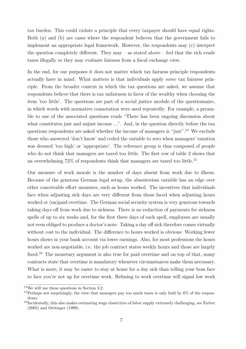
questions respondents are asked whether the income of managers is “just”.14 We exclude
those who answered ’don’t know’ and coded the variable to zero when managers’ taxation
was deemed ’too high’ or ’appropriate’. The reference group is thus composed of people
who do not think that managers are taxed too little. The first row of table 2 shows that
an overwhelming 72% of respondents think that managers are taxed too little.15
Our measure of work morale is the number of days absent from work due to illness.
Because of the generous German legal setup, the absenteeism variable has an edge over
other conceivable effort measures, such as hours worked. The incentives that individuals
face when adjusting sick days are very different from those faced when adjusting hours
worked or (un)paid overtime. The German social security system is very generous towards
taking days off from work due to sickness. There is no reduction of payments for sickness
spells of up to six weeks and, for the first three days of each spell, employees are usually
not even obliged to produce a doctor’s note. Taking a day off sick therefore comes virtually
without cost to the individual. The difference to hours worked is obvious: Working fewer
hours shows in your bank account via lower earnings. Also, for most professions the hours
worked are non-negotiable, i.e. the job contract states weekly hours and those are largely
fixed.16 The monetary argument is also true for paid overtime and on top of that, many
contracts state that overtime is mandatory whenever circumstances make them necessary.
What is more, it may be easier to stay at home for a day sick than telling your boss face
to face you’re not up for overtime work. Refusing to work overtime will signal low work
14We will use these questions in Section 3.2.15Perhaps not surprisingly, the view that managers pay too much taxes is only held by 6% of the respon-
dents.16Incidentally, this also makes estimating wage elasticities of labor supply extremely challenging, see Farber
(2005) and Oettinger (1999).
7
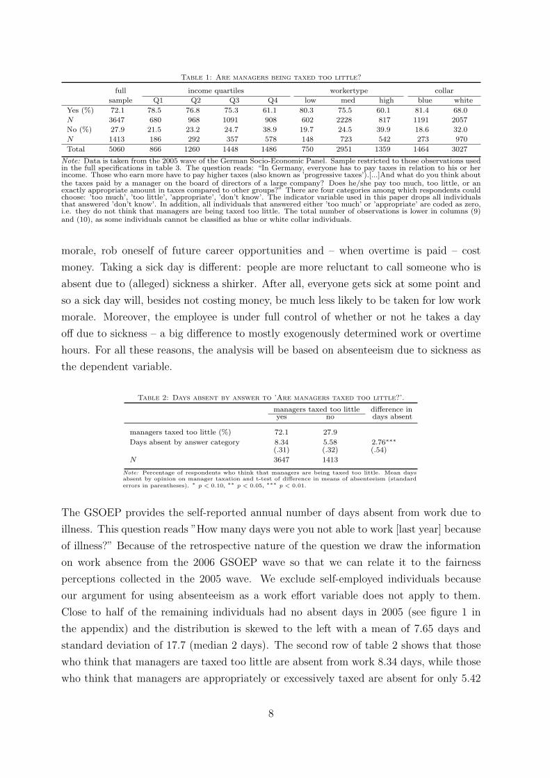
Table 1: Are managers being taxed too little?
full income quartiles workertype collar
sample Q1 Q2 Q3 Q4 low med high blue white
Yes (%) 72.1 78.5 76.8 75.3 61.1 80.3 75.5 60.1 81.4 68.0
N 3647 680 968 1091 908 602 2228 817 1191 2057
No (%) 27.9 21.5 23.2 24.7 38.9 19.7 24.5 39.9 18.6 32.0
N 1413 186 292 357 578 148 723 542 273 970
Total 5060 866 1260 1448 1486 750 2951 1359 1464 3027
Note: Data is taken from the 2005 wave of the German Socio-Economic Panel. Sample restricted to those observations usedin the full specifications in table 3. The question reads: “In Germany, everyone has to pay taxes in relation to his or herincome. Those who earn more have to pay higher taxes (also known as ’progressive taxes’).[...]And what do you think aboutthe taxes paid by a manager on the board of directors of a large company? Does he/she pay too much, too little, or anexactly appropriate amount in taxes compared to other groups?” There are four categories among which respondents couldchoose: ’too much’, ’too little’, ’appropriate’, ’don’t know’. The indicator variable used in this paper drops all individualsthat answered ’don’t know’. In addition, all individuals that answered either ’too much’ or ’appropriate’ are coded as zero,i.e. they do not think that managers are being taxed too little. The total number of observations is lower in columns (9)and (10), as some individuals cannot be classified as blue or white collar individuals.
morale, rob oneself of future career opportunities and – when overtime is paid – cost
money. Taking a sick day is different: people are more reluctant to call someone who is
absent due to (alleged) sickness a shirker. After all, everyone gets sick at some point and
so a sick day will, besides not costing money, be much less likely to be taken for low work
morale. Moreover, the employee is under full control of whether or not he takes a day
off due to sickness – a big difference to mostly exogenously determined work or overtime
hours. For all these reasons, the analysis will be based on absenteeism due to sickness as
the dependent variable.
Table 2: Days absent by answer to ’Are managers taxed too little?’.
managers taxed too little difference inyes no days absent
managers taxed too little (%) 72.1 27.9
Days absent by answer category 8.34 5.58 2.76∗∗∗
(.31) (.32) (.54)
N 3647 1413
Note: Percentage of respondents who think that managers are being taxed too little. Mean daysabsent by opinion on manager taxation and t-test of difference in means of absenteeism (standarderrors in parentheses). ∗ p < 0.10, ∗∗ p < 0.05, ∗∗∗ p < 0.01.
The GSOEP provides the self-reported annual number of days absent from work due to
illness. This question reads ”How many days were you not able to work [last year] because
of illness?” Because of the retrospective nature of the question we draw the information
on work absence from the 2006 GSOEP wave so that we can relate it to the fairness
perceptions collected in the 2005 wave. We exclude self-employed individuals because
our argument for using absenteeism as a work effort variable does not apply to them.
Close to half of the remaining individuals had no absent days in 2005 (see figure 1 in
the appendix) and the distribution is skewed to the left with a mean of 7.65 days and
standard deviation of 17.7 (median 2 days). The second row of table 2 shows that those
who think that managers are taxed too little are absent from work 8.34 days, while those
who think that managers are appropriately or excessively taxed are absent for only 5.42
8

days. This “fairness gap” of 2.92 days is highly statistically significant, and in relative
terms amounts to 39% of the average number of days absent. These observations are
consistent with the idea that individuals not only ’get angry’ when thinking about tax
breaks for the rich – as implied by the Economist poll mentioned above – but that there
are behavioral consequences to unjust taxation of the rich.
3 Estimation results
The descriptive statistics presented in section 2 show a positive correlation between the
belief that managers pay too little in taxes and days absent from work – a first indicator
that there may indeed be spillovers from tax fairness perceptions to work morale. The
GSOEP provides a vast array of control variables, far beyond what is usually available
in survey data, and this section provides estimates of the association between fairness
perceptions and absenteeism after netting out these possibly confounding factors. Our
benchmark is the linear OLS case, but due to the nature of the dependent variable, we
also use count-data and Quasi-Maximum-Likelihood methods. These estimations provide
the baseline results and give an idea of the magnitude of the ’fairness gap’, the difference
in sick days between two individuals who only differ in their assessment of whether or not
the rich pay their fair share in taxes. Section 3.2 then goes on to investigate whether this
fairness gap varies across population subgroups.
3.1 Baseline results
The main explanatory variable in all regressions of this subsection is the indicator variable
for whether an individual believes that ’managers are being taxed too little’, which we
take as a measure of whether taxation at the top of the income distribution is in line with
a respondent’s concept of fairness. We expect people holding this belief to respond by
increasing their days absent from work and thus the dependent variable is the number of
sick days in the year of the survey.17
17We exclude individuals who report more than 250 sick days, the maximum number of workdays per year.We could also have used a binary indicator of whether a person had at least one day of sick absence,however, finding an explanatory model for whether an individual has zero versus a positive number ofsick days is not actually what we are looking for. We believe the mechanism that we describe to workat any given number of sick days. That is, we are not interested in the effect of fairness perceptions onthe probability of not being sick for even one day, but rather we are interested in the effect on the totalnumber of sick days. It is probably easier for respondents to just ’add’ another day to sick days theyalready have. This practice may come with less feelings of guilt than taking the first day off withoutactually being sick. This leads us to expect a rather small effect in the dummy dependent variablecase. Probit estimations not reported here confirm this. Believing that manager taxation is unfair has a
9

Table 3 provides the results from linear OLS estimations.18 Column (1) reproduces the
raw differential presented in table 2 by using a bivariate regression model: People who
think that managers are taxed too little report on average 2.9 more days of staying away
from work due to illness. A first natural candidate to control for is a person’s individual
health.19 It might be argued that the correlation of Column (1) is driven by reversed
causality: Those who stay at home due to illness may become aware that they are net
benefiters of the social security system and therefore always think that taxation levels are
too low. Column (2) therefore adds two indicators of respondents’ health status. Health
score is a self-reported assessment of an individual’s objective health status. Respondents
can rate their health on a scale ranging from ’poor’ [1] to ’very good’ [5]. However, there
may be vast differences in the health threshold that needs to be reached before a person
decides to call in sick. Hence, we also control for the subjective satisfaction with health
status. This variable is coded on an 11-point scale ranging from ’totally unhappy’ [0] to
’totally happy’ [10]. Both variables are significant and the coefficients bear the expected
negative sign. They imply that better objective health leads to lower levels of absenteeism,
and that at fixed objective health, higher levels of satisfaction with this particular level
of well-being are associated with lower absenteeism.20 Most interestingly, the difference
in absenteeism after controlling for health is still two full days, compared to the 2.9 days
difference in absenteeism without any controls.
Individual income is also an important control variable. One can argue that low-income
earners may systematically want higher tax levels for the rich, and that they also have
a higher probability of shirking, as they have less at stake when getting caught. Since
this would bias our coefficient of interest upwards, income is included in column (3) along
with other personal characteristics, some of which would be included in a standard Mincer
equation. It turns out that a higher level of education is associated with fewer sick days,
as is advanced age and having children. However, the belief that the tax system at the
upper end of the income distribution is unfair is still associated with significantly higher
levels of absenteeism, despite the number being cut down to one sick day. Adding job and
firm related variables in columns (4) and (5) does not further diminish the tax fairness
coefficient, the difference in absenteeism now actually increases somewhat. Longer job
tenure and larger firm size are both associated with higher levels of absenteeism. A
marginal effect of 0.041 in the full specification, i.e. the perception of an unfair tax system is associatedwith a four percent higher probability of having at least one sick day.
18Table 7 in the appendix gives descriptions of all the variables used in this paper, and table 8 in theappendix displays summary statistics.
19In fact, if everyone used sick days the way one is supposed to, there should not be any systematicpredictors of absenteeism other than actual health.
20Obviously, both these variables are of a subjective nature, even if the health score variable asks for anobjective level of well-being. We would of course prefer to have a really objective measure, such as theresults from getting a physical at a doctor’s office. However, such data are not available.
10

possible explanation would be that longer tenure makes it harder for employers to punish
shirking due to lay-off protection laws, while a larger firm size reduces the probability
of getting caught while shirking. From column (4) on, the specifications also include 16
indicators for the German regions and 9 indicators representing an individual’s rank in
the firm’s hierarchy – the former for netting out regional differences in work attitudes
among others, the latter as further controls for socio-economic status.
The GSOEP allows us to account for some personal attitudes and mental states directly,
rather than using proxies for them. After adding these variables in column (6) the ab-
senteeism difference increases somewhat to 1.5 days and remains highly significant. We
control for whether someone is satisfied with his job, since the job related and firm related
variables we included above may not fully capture workplace characteristics driving both
work morale and attitudes towards taxing the rich. Lower job satisfaction can reduce
an indiviudal’s work morale and may be the result of antipathy against own superiors,
who individuals may equate with the “rich” or the ”managers”. We also include fear of
job loss, although perceived job security may already be partly covered by the dummies
for part-time and marginally employed. It can also be argued that the correlation be-
tween sick absence and the belief that managers are taxed insufficiently is spurious due
to a self-serving bias: Those who often stay at home may do so because of their laziness,
and in order to justify their own deficiencies, these respondents accuse managers of being
immoral by saying that they are not paying their dues. To meet this objection, we also
control for an individual’s self-reported laziness (on a scale from 0 to 7). Still, people
may be reluctant to answer this question truthfully. However, the absenteeism question
inquires about sick days in the past year and is thus taken from the 2006 GSOEP wave,
whereas the laziness question as well as all other variables are from the 2005 wave. The
fact that absenteeism varies quite a bit over the two waves should thus substantially miti-
gate this potential self-servingness. Finally, we take into account a person’s degree of risk
aversion, as shirking is a still a risky behavior even under the high job protection levels in
Germany. Somewhat surprisingly, none of these soft variables have a significant associa-
tion with absenteeism. The other controls may already account for these characteristics,
e.g. it is likely that certain individuals select themselves into certain industries or firms.
The gap associated with differing perceptions of tax fairness is apparently very robust to
the specification chosen and hardly changes at all after the inclusion of health and personal
characteristics. The main message of these estimates is that the connection between tax
fairness beliefs and absenteeism, described in section 2, does not seem to be an artefact
of failing to control for these observable characteristics.
The fact that the dependent variable can only take on non-negative integer values means
11

Table
3:
OL
S,
dependent
varia
ble
days
abse
nt.
(1)
(2)
(3)
(4)
(5)
(6)
man
ager
sta
xed
too
litt
le2.9
15∗∗
∗(0.3
94)
2.0
13∗∗
∗(0.3
72)
1.1
71∗∗
∗(0.4
09)
1.2
77∗∗
∗(0.4
36)
1.3
57∗∗
∗(0.4
53)
1.5
41∗∗
∗(0.4
47)
hea
lth
score
−3.3
92∗∗
∗(0.4
13)
−3.3
82∗∗
∗(0.4
53)
−3.2
83∗∗
∗(0.4
70)
−3.4
73∗∗
∗(0.4
90)
−3.3
17∗∗
∗(0.4
86)
hea
lth
sati
sfact
ion
−.8
846∗∗
∗(0.1
86)
−.9
287∗∗
∗(0.2
01)
−.9
905∗∗
∗(0.2
08)
−.9
619∗∗
∗(0.2
15)
−1.0
51∗∗
∗(0.2
38)
Pers
onalchara
cte
rist
ics
gro
ssin
com
e.0
439
(0.1
09)
−.0
871
(0.1
24)
−.2
121
(0.1
32)
−.1
621
(0.1
30)
age
−.3
146∗∗
(0.1
40)
−.3
523
(0.2
28)
−.4
602∗
(0.2
50)
−.2
535
(0.2
38)
ages
q.0
037∗∗
(0.0
02)
.0047
(0.0
03)
.0062∗
(0.0
03)
.0032
(0.0
03)
male
−.7
615
(0.5
11)
−.9
9(0.6
30)
−1.1
9∗
(0.6
62)
−.7
492
(0.6
42)
child
ren
−1.1
65∗∗
(0.4
61)
−.6
608
(0.5
08)
−.5
138
(0.5
33)
−.5
237
(0.5
37)
fore
ign
1.7
99
(1.2
69)
1.9
83
(1.3
21)
1.9
13
(1.3
92)
.8479
(1.1
98)
sch
oolin
g−.3
972∗∗
∗(0.0
83)
−.3
582∗∗
∗(0.1
34)
−.3
166∗∗
(0.1
38)
−.3
312∗∗
∗(0.1
25)
Job
rela
ted
vari
able
ste
nu
re.2
354∗∗
∗(0.0
82)
.2179∗∗
∗(0.0
84)
.1966∗∗
(0.0
84)
tenu
resq
−.0
067∗∗
∗(0.0
02)
−.0
068∗∗
∗(0.0
02)
−.0
062∗∗
∗(0.0
02)
full
tim
eex
per
ien
ce−.1
406
(0.1
37)
−.1
693
(0.1
42)
−.1
914
(0.1
35)
full
tim
eex
per
ien
cesq
.0029
(0.0
03)
.0032
(0.0
03)
.0049
(0.0
03)
part
tim
eex
per
ien
ce.0
848
(0.1
61)
.054
(0.1
65)
.0822
(0.1
39)
part
tim
eex
per
ien
cesq
−.0
054
(0.0
04)
−.0
049
(0.0
04)
−.0
04
(0.0
04)
part
tim
e(a)
−1.6
94∗
(0.9
65)
−1.4
49
(1.0
32)
−1.4
07
(1.0
15)
marg
inally
emp
loyed
−6.4
92∗∗
∗(1.1
67)
−6.4
59∗∗
∗(1.2
01)
−6.3
1∗∗
∗(1.2
23)
Fir
mle
velvari
able
s
20<
emp
loyee
s<200
(b)
1.5
46∗∗
(0.6
99)
1.5
79∗∗
(0.7
14)
200<
=em
plo
yee
s<2000
3.6
96∗∗
∗(0.8
08)
3.2
24∗∗
∗(0.7
96)
emp
loyee
s>2000
3.0
79∗∗
∗(0.7
08)
2.8
49∗∗
∗(0.7
12)
agri
cult
ure
(c)
−3.3
85∗∗
(1.5
30)
−3.2
24∗∗
(1.5
21)
min
ing/en
ergy
4.6
06
(2.8
65)
5.2
5∗
(2.9
67)
pro
cess
ing
−.4
616
(0.9
24)
−.0
545
(0.9
00)
traffi
c/m
edia
.8531
(1.0
79)
.7244
(1.0
33)
con
stru
ctio
n1.8
19
(1.5
65)
2.0
45
(1.6
10)
wh
ole
sale
1.3
68
(1.0
75)
1.6
41
(1.0
87)
serv
ices
−.4
73
(0.7
62)
−.3
028
(0.7
43)
ban
kin
g/in
sura
nce
−.1
163
(0.9
45)
.3499
(0.9
46)
pu
blic
sect
or
.2814
(0.8
03)
.6824
(0.7
52)
Pers
onalattitudes
afr
aid
tolo
sejo
b−.0
953
(0.5
07)
sati
sfied
w/
job
.0476
(0.1
72)
lazy
−.1
02
(0.1
57)
risk
taker
.0538
(0.1
24)
con
stant
5.4
25
(0.2
70)
24.4
4(1.5
19)
37.3
4(3.4
21)
36.9
9(4.8
14)
37.4
6(5.3
01)
33.5
4(5.3
07)
16
regio
nd
um
mie
sN
oN
oN
oY
esY
esY
es9
occ
up
ati
on
du
mm
ies
No
No
No
Yes
Yes
Yes
log-L
ikel
ihood
-3.2
e+04
-3.2
e+04
-2.4
e+04
-2.4
e+04
-2.2
e+04
-2.1
e+04
R2
0.0
10.0
57
0.0
71
0.0
80
0.0
88
0.0
88
N7327
7304
5773
5535
5217
5060
Note
:S
tan
dard
erro
rsin
pare
nth
eses
allow
for
clu
ster
ing
at
the
hou
seh
old
level
.R
efer
ence
cate
gori
esare
:(a
)fu
ll-t
ime
for
’job
statu
s’,
(b)
less
than
20
emp
loyee
sfo
r’fi
rmsi
ze’,
(c)
manu
fact
uri
ng
for
’sec
tora
ld
um
mie
s’.
Colu
mn
s(1
)-(6
)are
stan
dard
lin
ear
OL
Sre
gre
ssio
ns
wit
hd
epen
den
tvari
ab
le’n
um
ber
of
days
ab
sent’
.∗
p<
0.1
0,∗∗p<
0.0
5,∗∗
∗p<
0.0
1.
12

that OLS is not the preferred method of estimation and count-data methods are a better
fit. This is why table 4 presents results from a Poisson model, a Negative Binomial (Neg-
bin II) model, and a two-step Negative Binomial Quasi Maximum Likelihood Estimator
(QMLE). While the first two of these models are fairly standard count-data models, the
third was proposed by Wooldridge (2002) and has desirable robustness properties. The
QMLE estimator is a fully robust estimator in the sense that it does not rely on the
distributional assumption and the variance assumption of the Negbin II model. Only the
conditional mean assumption is needed for consistency.21 In the Poisson model shown
in column (1) all control variables have significant coefficients. However, due to overdis-
persion in the dependent variable – which can be inferred from the estimate of η2 in the
two other models – the standard errors produced by the Poisson model systematically
underestimate the true standard errors. Inference should therefore be based on the Neg-
ative Binomial and QMLE models. Coefficients must be interpreted as in a log-linear
regression, and the preferred QMLE model estimates the difference in absenteeism at
26%, which translates to roughly 2 days of absenteeism – somewhat more than the OLS
estimates in column (6) of the previous table suggested. This again emphasizes the very
robust nature of the fairness gap and establishes that individuals who perceive the tax
system to be unfair have a much higher level of absenteeism, even after conditioning on
a vast array of possible confounders.
3.2 Subgroups - taxation and relative deprivation
In this section we analyze whether the connection between perceived unfairness in taxing
the rich and willingness to comply with work norms is a “local” phenomenom or whether
it is found through a wide range of socio-economic classes. Table 5 presents the QMLE
results for various subsamples. To begin with, it has been frequently observed in the social
comparisons literature that women and men are differently affected by violations of social
norms (see e.g. Clark, 2003). Interestingly, the association of the belief that managers
are taxed too little with our chosen measure of work effort does not systematically differ
between genders as is suggested in the top panel of table 5 – the fairness gap is very
similar for men and women. This is not the case when blue and white collar workers are
considered: The fairness gap is almost twice as large as for blue collar workers than for
those working in white collar jobs. Yet, in both subgroups the coefficient on tax unfairness
is highly significant.
To further check whether socio-economic status matters, we split the sample up along
21See Wooldridge (2002) for details.
13
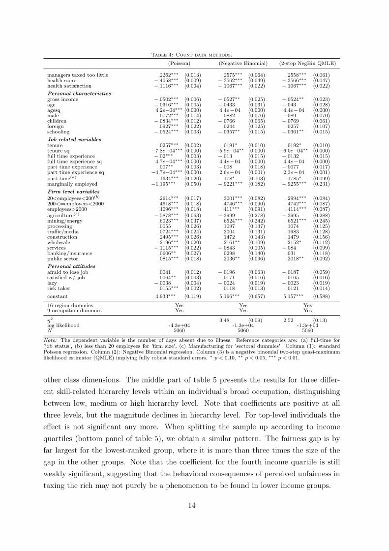
Table 4: Count data methods.
(Poisson) (Negative Binomial) (2-step NegBin QMLE)
managers taxed too little .2262∗∗∗ (0.013) .2575∗∗∗ (0.064) .2558∗∗∗ (0.061)health score −.4058∗∗∗ (0.009) −.3562∗∗∗ (0.049) −.3566∗∗∗ (0.047)health satisfaction −.1116∗∗∗ (0.004) −.1067∗∗∗ (0.022) −.1067∗∗∗ (0.022)
Personal characteristicsgross income −.0502∗∗∗ (0.006) −.0527∗∗ (0.025) −.0524∗∗ (0.023)age −.0316∗∗∗ (0.005) −.0433 (0.031) −.043 (0.028)agesq 4.2e−04∗∗∗ (0.000) 4.4e−04 (0.000) 4.4e−04 (0.000)male −.0772∗∗∗ (0.014) −.0882 (0.076) −.089 (0.070)children −.0834∗∗∗ (0.012) −.0766 (0.065) −.0769 (0.061)foreign .0927∗∗∗ (0.022) .0244 (0.125) .0257 (0.107)schooling −.0524∗∗∗ (0.003) −.0357∗∗ (0.015) −.0361∗∗ (0.015)
Job related variablestenure .0257∗∗∗ (0.002) .0191∗ (0.010) .0192∗ (0.010)tenure sq −7.8e−04∗∗∗ (0.000) −5.9e−04∗∗ (0.000) −6.0e−04∗∗ (0.000)full time experience −.02∗∗∗ (0.003) −.013 (0.015) −.0132 (0.015)full time experience sq 4.7e−04∗∗∗ (0.000) 4.4e−04 (0.000) 4.4e−04 (0.000)part time experience .007∗∗ (0.003) −.008 (0.018) −.0077 (0.017)part time experience sq −4.7e−04∗∗∗ (0.000) 2.6e−04 (0.001) 2.3e−04 (0.001)part time(a) −.1634∗∗∗ (0.020) −.178∗ (0.103) −.1785∗ (0.099)marginally employed −1.195∗∗∗ (0.050) −.9221∗∗∗ (0.182) −.9255∗∗∗ (0.231)
Firm level variables
20<employees<200(b) .2614∗∗∗ (0.017) .3001∗∗∗ (0.082) .2994∗∗∗ (0.084)200<=employees<2000 .4618∗∗∗ (0.018) .4746∗∗∗ (0.090) .4742∗∗∗ (0.087)employees>2000 .4096∗∗∗ (0.018) .411∗∗∗ (0.091) .4114∗∗∗ (0.087)agriculture(c) −.5878∗∗∗ (0.063) −.3999 (0.278) −.3995 (0.288)mining/energy .6023∗∗∗ (0.037) .6524∗∗∗ (0.242) .6521∗∗∗ (0.245)processing .0055 (0.026) .1097 (0.137) .1074 (0.125)traffic/media .0724∗∗∗ (0.024) .2004 (0.131) .1983 (0.128)construction .2495∗∗∗ (0.026) .1472 (0.143) .1479 (0.156)wholesale .2196∗∗∗ (0.020) .2161∗∗ (0.109) .2152∗ (0.112)services −.1115∗∗∗ (0.022) −.0843 (0.105) −.084 (0.099)banking/insurance .0606∗∗ (0.027) .0298 (0.140) .031 (0.118)public sector .0815∗∗∗ (0.018) .2036∗∗ (0.096) .2018∗∗ (0.092)
Personal attitudesafraid to lose job .0041 (0.012) −.0196 (0.063) −.0187 (0.059)satisfied w/ job .0064∗∗ (0.003) −.0171 (0.016) −.0165 (0.016)lazy −.0038 (0.004) −.0024 (0.019) −.0023 (0.019)risk taker .0155∗∗∗ (0.002) .0118 (0.013) .0121 (0.014)
constant 4.933∗∗∗ (0.119) 5.166∗∗∗ (0.657) 5.157∗∗∗ (0.588)
16 region dummies Yes Yes Yes9 occupation dummies Yes Yes Yes
η2 3.48 (0.09) 2.52 (0.13)log likelihood -4.3e+04 -1.3e+04 -1.3e+04N 5060 5060 5060
Note: The dependent variable is the number of days absent due to illness. Reference categories are: (a) full-time for’job status’, (b) less than 20 employees for ’firm size’, (c) Manufacturing for ’sectoral dummies’. Column (1): standardPoisson regression. Column (2): Negative Binomial regression. Column (3) is a negative binomial two-step quasi-maximumlikelihood estimator (QMLE) implying fully robust standard errors. ∗ p < 0.10, ∗∗ p < 0.05, ∗∗∗ p < 0.01.
other class dimensions. The middle part of table 5 presents the results for three differ-
ent skill-related hierarchy levels within an individual’s broad occupation, distinguishing
between low, medium or high hierarchy level. Note that coefficients are positive at all
three levels, but the magnitude declines in hierarchy level. For top-level individuals the
effect is not significant any more. When splitting the sample up according to income
quartiles (bottom panel of table 5), we obtain a similar pattern. The fairness gap is by
far largest for the lowest-ranked group, where it is more than three times the size of the
gap in the other groups. Note that the coefficient for the fourth income quartile is still
weakly significant, suggesting that the behavioral consequences of perceived unfairness in
taxing the rich may not purely be a phenomenon to be found in lower income groups.
14

Table 5: 2-step QMLE estimations, subsamples.
by sex(a) by worker class(b)
(male) (female) (blue collar) (white collar)
managers taxed too little .2078∗∗∗ .2397∗∗∗ .3725∗∗∗ .1963∗∗∗
(0.078) (0.088) (0.121) (0.074)N 2858 2202 1464 3027
by hierarchy in occupation(c)
(low) (medium) (high)
managers taxed too little .5216∗∗∗ .2009∗∗∗ .1595(0.147)) (0.077) (0.104)
N 750 2951 1359
by income quartile(d)
(1st Q) (2nd Q) (3rd Q) (4th Q)
managers taxed too little .6106∗∗∗ .1658 .189∗ .1884∗
(0.168) (0.108) (0.098) (0.101)N 866 1260 1448 1486
Note: The full sample is split by: (a) male and female respondents, (b) blue and white collar respondents, (c)three skill-related hierarchy levels in occupation, (d) income quartiles of the 2005 SOEP wave. All estimationsare two-step quasi-maximum likelihood (QMLE) implying fully robust standard errors. The dependent variable is’number of days absent’. ∗ p < 0.10, ∗∗ p < 0.05, ∗∗∗ p < 0.01.
The finding that the coefficient of the manager taxation indicator is larger in size for
lower ranked individuals and that it tends to decrease when moving up the social ladder
is consistent with the concept of relative deprivation (Runciman, 1966), which has recently
attracted attention among economists in the social comparisons literature (see e.g. Ferrer-
i-Carbonell, 2005). This concept stipulates that individuals feel grievance when others
possess things oneself does not have (but feels entitled to), and this grievance rises with
distance to the privileged social group. To the extent that greater grievance is also
accompanied by greater behavioral responses, our result that low-income individuals react
more strongly to perceived tax privileges of the rich are well in line with this hypothesis.
In our case the trigger of relative deprivation has a different dimension from the one along
which deprivation rises - the trigger is of the dimension “tax payments” while the extent
of deprivation is related to “rank” on a positional scale. That comparison processes may
go well beyond one-dimensional comparisons of income has been shown by Abeler et al.
(2009).
4 Alternative fairness concepts, preference for redis-
tribution, and ’complainer attitudes’.
In the previous section, we have uncovered a strong association between perceived unfair-
ness in taxing the rich and absenteeism, which holds even after conditioning on a consid-
erable number of observable characteristics and throughout most of the subsamples. In
this section, we address the issue of potential remaining unobserved heterogeneity. Par-
ticularly, we look into whether fairness concepts other than tax fairness may drive our
15

manager-taxed-too-little coefficient.
So far we haven’t considered the respondents’ own tax burden. It may be argued that
the belief that managers pay too little in taxes is positively related to one’s own tax
rate. Then, the coefficients on manager taxation presented so far may be confounded
with another mechanism that is independent from fairness considerations at all: a higher
tax rate reduces an individual’s net income or, equivalently, the expected loss from being
detected, which calls for higher levels of shirking according to a standard neoclassical
model. The GSOEP allows us to calculate the average tax rate individuals effectively face.
Respondents are asked for the gross as well as for the net income. We take the difference
between these two variables and divide it by gross income. This effective average tax rate
is included as an additional regressor. As a benchmark, column (1) of table 6 reproduces
the effect from the full specification of the QMLE model from the last column of table
4. Column (2) shows the results when the effective average tax rate is added (only the
coefficient of the additional regressors and manager taxation are shown in this table). The
effect of the tax unfairness indicator remains very stable.
A related issue is that the question on manager taxation explicitly asks the respondent
to evaluate the tax burden of the rich in comparison to ’other groups’. Hence, it could be
argued that labeling managers’ tax burden as ’too low’ may be just another way of stating
that your own tax burden is unfairly high. The overall aim of this paper is to provide
evidence that perceived injustice in taxation may spill over to other areas than taxation
itself. For this purpose, it is irrelevant why individuals think the rich are being taxed too
little. All we need is the assumption that the source of this belief is indeed perceived tax
unfairness. If however, the argument equates tax fairness to income fairness (stating that
own taxation is unfairly high may be equivalent to stating that own net income is unfairly
low), we need further controls.
The conjecture that tax fairness coincides with concepts of income fairness and that it is
this kind of fairness that drives our results is a fundamental objection, since ultimately
it questions whether tax fairness presents a distinct fairness category at all.22 However,
22It should be emphasized that discussions of the fairness of taxation are an integral part of mainstreampublic economics. A discussion of the principles of just taxation is found in many textbooks of publicfinance. For example, in what could be called the epitome of public economics textbooks, Musgrave(1959) devotes two entire chapters to tax equity issues. An example that illustrates how dedicated thesediscussions can be is the so called Musgrave/Kaplow Exchange. Starting in one, then continued in anotherjournal, Musgrave and Kaplow debated over four years on whether the concept of horizontal tax equityhas any normative significance aside from vertical equity and on how these equity concepts relate to thegoal of efficiency. (The Musgrave/Kaplow Exchange refers to Kaplow, 1989, Musgrave, 1990, Kaplow,1992 and Musgrave 1993.) Clearly, the discussion on wether tax equity has any normative significancebesides other principles is not a strict proof of its relevance for individual behavior, but it is anotheranecdotal evidence that people are not unaffected by tax equity considerations.
16

Table
6:
Robust
ness
checks.
(1)
(2)
(3)
(4)
(5)
(6)
(7)
(8)
(9)
(10)
man
ager
sta
xed
too
litt
le.2
558∗∗
∗.2
41∗∗
∗.2
566∗∗
.1783∗∗
.2572∗∗
∗.2
532∗∗
∗.2
532∗∗
∗.2
534∗∗
∗.1
608∗∗
.2111∗∗
∗
(0.0
61)
(0.0
61)
(0.0
61)
(0.0
73)
(0.0
61)
(0.0
61)
(0.0
61)
(0.0
61)
(0.0
75)
(0.0
74)
effec
tive
aver
age
tax
rate
−.1
152
−.3
453
(0.2
92)
(0.3
66)
ow
nin
com
eu
nfa
ir−.0
042
.012
(0.0
59)
(0.0
72)
man
ager
inco
me
un
fair
.1936∗∗
.1816∗∗
(0.0
77)
(.077)
left
ist/
right
−.0
067
−.0
314∗
(0.0
16)
(0.0
19)
inco
me
det
erm
ined
by
luck
.1444∗∗
.0575
(0.0
63)
(0.0
79)
pes
sim
ist
−.0
014
−.0
969
(0.0
62)
(0.0
76)
life
sati
sfact
ion
−.0
087
.0189
(0.0
21)
(0.0
25)
59
contr
ols
Yes
Yes
Yes
Yes
Yes
Yes
Yes
Yes
Yes
Yes
N5060
4983
5045
3391
4978
5043
5048
5056
3267
3267
Note
:A
lles
tim
ati
on
sare
two-s
tep
qu
asi
-maxim
um
likel
ihood
esti
mato
rs(Q
ML
E)
imp
lyin
gfu
lly
rob
ust
stan
dard
erro
rs.
Th
ed
epen
den
tvari
ab
leis
the
nu
mb
erof
days
ab
sent
du
eto
illn
ess
an
dvari
ou
sad
dit
ion
al
contr
ols
are
ad
ded
toth
efu
llsp
ecifi
cati
on
inth
eco
unt
data
mod
els.
Colu
mn
(1)
show
sth
ere
fere
nce
coeffi
cien
tfr
om
tab
le4.
Colu
mn
(2)
ad
ds
the
resp
on
den
t’s
effec
tive
aver
age
tax
rate
,co
lum
n(3
)ad
ds
an
ind
icato
rfo
rw
het
her
the
ind
ivid
ual
per
ceiv
esh
isow
nin
com
eto
be
un
fair
,co
lum
n(4
)ad
ds
an
ind
icato
rfo
rw
het
her
the
ind
ivid
ual
per
ceiv
esm
an
ager
s’in
com
esto
be
un
fair
,co
lum
n(5
)ad
ds
avari
ab
leth
at
mea
sure
sth
ere
spon
den
t’s
posi
tion
wit
hin
the
politi
cal
spec
tru
m(l
ow
ervalu
esin
dic
ate
ale
ftis
tst
an
ce),
colu
mn
(6)
ad
ds
an
ind
icato
rfo
rw
het
her
the
resp
on
den
tb
elie
ves
that
inco
me
ism
ost
lyd
eter
min
edby
luck
,co
lum
n(7
)in
clu
des
an
ind
icato
rfo
rw
het
her
the
resp
on
den
tis
pes
sim
isti
cab
ou
tth
efu
ture
,co
lum
n(8
)ad
ds
avari
ab
leth
at
mea
sure
sh
ow
sati
sfied
the
resp
on
den
tis
wit
hlife
over
all
(hig
her
valu
esin
dic
ate
hig
her
sati
sfact
ion
level
s),
the
spec
ifica
tion
inco
lum
n(9
)in
clu
des
all
ad
dit
ion
alvari
ab
les.
Bec
au
seth
ein
clu
sion
of
the
’man
ager
s’in
com
e’qu
esti
on
sign
ifica
ntl
yre
duce
sth
esa
mp
lesi
ze,
colu
mn
s(4
)an
d(9
)ca
nn
ot
be
com
pare
dto
colu
mn
(1).
To
allow
for
aco
mp
ari
son
,w
ead
dre
fere
nce
colu
mn
(10),
wh
ich
show
sth
ere
fere
nce
coeffi
cien
tw
hen
the
spec
ifica
tion
from
colu
mn
(1)
ises
tim
ate
don
this
smaller
sam
ple
from
colu
mn
(9).
∗p<
0.1
0,∗∗p<
0.0
5,∗∗
∗p<
0.0
1.
17

the SOEP provides us with the luxury to control also for income fairness beliefs. Fairness
perceptions of own wage income are collected in the GSOEP by asking ”Is the income
that you earn at your current job just, from your point of view? [Yes/No].” The third
column of table 6 shows the coefficient of fairness perceptions of manager taxes in the
overall sample after including this variable. When compared to the benchmark coefficient
shown in column (1), the coefficient of tax fairness beliefs remains virtually unaltered in
column (3). In other words, these results do not suggest that an evaluation of managers’
taxes as being too low is confounded with perceiving one’s own income as unjust. The
GSOEP also allows us to control for whether individuals think managers earn too much.
It asked its is participants ”How high on average is the monthly net income of a manager
on the board of directors of a large company? Would you say that this income has a just
relation to the job demands? [Yes/No]”. As can be seen in column (4), the perception of
manager incomes as unfair is also associated with a higher number of days absent, yet the
coefficient on manager taxation still suggests a 18% higher level of absenteeism for those
who believe the tax system to be unfair. The coefficient is not as precisely estimated as
before, yet still significant at the 5% level. The imprecision stems in part from the way
this question is asked: respondents were only asked the fairness part if they could specify
how much they think managers earn. This causes a drop in the number of observations
by roughly one third. Due to the samples being different, the coefficient on manager
taxation should not be compared to the benchmark in column (1). Rather, in column
(10) we show a benchmark coefficient from a QMLE estimation of the specification shown
in column (1), estimated on the restricted sample that results from the non-responses
to the ’manager income fairness’ question. This coefficient in column (10) is 0.21, and
so the drop to 0.18 in column (4) suggests that 85% of the original effect remain. This
large part of the original coefficient then cannot be due to perceiving managers income to
be unfair. In the end, this finding gives us some confidence that, while tax fairness and
income fairness may have some overlap, our “the rich-don’t-pay-their-share” coefficient is
not confounded by income fairness.
A related concern is whether a preference for redistribution may be confounded with
the manager tax coefficient, too. Someone who states that the rich are taxed too little
may in essence be concerned about insufficient levels of redistribution from the rich to
other parts of the population. In column (5), we thus add a control for the respondent’s
position within the political spectrum. Lower values indicate a leftist stance, which can be
assumed to go with a preference for redistribution. Because preferences for redistribution
are not necessarily fully captured in political views, column (6) includes an indicator for
whether the respondent believes that income is mostly determined by luck. The notion
that one’s position in the income distribution is a matter of fate can be accompanied by
18

a propensity to support redistributive policies, e.g. because beliefs also imply little trust
in upward social mobility (Piketty 1995; Alesina and Giuliano, 2009). While the political
views do not show a significant coefficient, believing in luck as the determinant of income
is significantly associated with 14% more sick days.23 Interestingly, the association of a
preference for redistribution with absenteeism seems to be independent of the tax fairness
perceptions – which still indicate 25% higher levels of absenteeism.
Finally, some individuals may have a negative attitude towards many things in general.
Such attitudes may in part be triggered by being sick often, and also lead individuals
to assess the taxation of others as unfair – as a way of expressing a generally negative
stance. Aside from this reverse causality, pessimism acts as another variable that captures
beliefs about social mobility. Column (8) adds a variable which indicates whether the
respondent is ’pessimistic about the future’. From the coefficient, it seems seems that
such a disposition is unrelated to absenteeism and tax fairness. There is some importance
to this result: finding pessimism to be a confounder of the tax fairness coefficient would
have meant that it is not even another fairness category driving our results, but rather
a negative view of life prospects. Other individuals may loosely be termed ’complainers’.
Their ’complainer’ attitude may cause them to lament about the tax system more often
and at the same time be associated with having more sick days. To the extent that such
attitudes are not fully captured in the ’pessimist’ control variable, they can still bias our
estimates. As a further robustness check we therefore use a GSOEP question on general
life satisfaction. The question reads: “How satisfied are you with your life, all things
considered? [scale 0-10]”. The results after including this additional regressor are shown
in column (9) of table 6, where the coefficient on manager taxation remains stable and
precise. The fact that being dissatisfied with life in general is not associated with more sick
days suggests that the control variables of the benchmark specification are already holding
all relevant factors constant that life satisfaction might proxy for. Another reason for this
association to be be insignificant could be that life satisfaction does not meet the criteria
to be a valid proxy variable. If there is some idiosyncratic variation in life satisfaction
that makes it deviate temporarily from the underlying unobserved ’complainer’ attitude,
then life satisfaction is not an appropriate proxy variable, but rather an indicator variable
(see Wooldridge 2002, p. 105). A way to correct for such variation in an indicator
variable has been proposed by Griliches and Mason (1972), see also Griliches (1977),
Chamberlain (1977) and Blackburn/Neumark (1993, 1995). It involves instrumenting
23This is interesting in its own. Alesina and Angeletos (2005) introduce the disutility stemming fromthe perception that luck determines income in a additive-separable manner, and hence, as having nobehavioral affects. The question of how to introduce fairness into standard neoclassical utility functionsis a question not adressed in this paper. However, our results can also be seen as evidence for justifyingincentive shaping variants.
19

life satisfaction with a second measure for the underlying unobserved factor, which must
not be correlated with the variation in life satisfaction that makes it fluctuate around
the underlying ’complainer’ attitude. We choose values of life satisfaction lagged by one
period and lagged by five periods as instruments, employing them both separately in
two different specifications. The longer lag length accommodates the case in which the
shocks that make life satisfaction deviate from the underlying attitude last over several
years (Clark et al. 2008). Table 9 in the appendix shows that both lagged values of
life satisfaction are sufficiently correlated with contemporaneous life satisfaction in the
first stage regression, and that the coefficient on manager taxation remains stable after
instrumenting. Column (9) of table 6 jointly includes all additional controls discussed in
this section. The manager tax fairness coefficient is still significant and not much smaller
than the benchmark in column (10).
For the income and status sub-groups presented earlier, the same robustness checks (not
reported here) deliver qualitatively very similar results as before, i.e., for workers in the
first quartile of the wage distribution, the effect is generally high and significant, while it
is lower and not significant for workers in the higher quartiles, and for blue collar workers
the effect is stronger than for white collar workers. Overall, this section shows that the
correlation between tax fairness perceptions and absenteeism is not due to preferences for
redistribution or alternative fairness concepts. There is also little evidence to suggest the
coefficient may be biased due to unobserved heterogeneity caused by being pessimistic in
general or having a ’complainer’ personality.
5 Conclusion
Everybody knows someone who complains about injustice in taxing the rich. Whether
such complaints translate into behavior is the core question of this paper. We use a large
scale German data set and investigate whether the belief that the rich don’t pay a sufficient
amount of taxes affects work morale. The results provide first evidence suggesting that:
(a) there is indeed a connection between an agent’s complaining over injustice in taxing
the rich and his propensity to work hard, and (b) this connection is surprisingly strong.
On average, the belief that the top income earners don’t contribute a fair share in taxes is
associated with a 20 percent increase in days absent from work due to illness, our measure
of work morale. The results prove robust to adding standard labor economics controls as
well as a wide variety of individual attitudes that may affect absenteeism but that are not
generally available in other data sets.
20

The contribution of this paper is twofold. First, we deal with the question of how taxes
affect the economy. It is standardly assumed that taxes deter economic activity via
reduced monetary incentives. We provide evidence that perceived injustice in taxation
may crowd out effort as well. Second, and at a more general level, we build on the recent
economic literature on fairness. Not only are our results well in line with the established
hypothesis that in addition to material self-interest, fairness matters for economic behavior
– we also add several new aspects to this literature. Most importantly, responses to
perceived injustice in a certain area may not be restricted to that area, but rather ’fairness
spillovers’ may be present. In addition, these responses – though indirect – may be
substantial and associated with large economic costs.
One reason why we found relatively large effects may be the following. It is considered a
stylized fact that Europeans believe success to be a matter of luck rather than of hard work
(Alesina and Angeletos, 2005), and that Europeans generally believe social mobility to be
low (Benabou and Tirole, 2006). Thus, it can be assumed that in Germany, grievance over
not belonging to the upper social strata is rather high, and so people may be especially
averse to tax breaks for the wealthy. It should be interesting to see, whether in a country
like the United States, where people believe in social mobility and in being in charge of
their own destiny, the effect of perceived unfairness of taxation on work effort is smaller.
Provided that the effects can be shown to be undoubtedly causal – a task left for future
research – they suggest that the excess burden of taxation may be quite different from
what is usually assumed. Traditionally, welfare costs of taxation are assessed in terms
of distorting monetary incentives. However, our analysis revealed that there are other
channels through which tax policy may have an impact on economic behavior. Neglecting
these fairness-induced costs of taxation bears the risk of arriving at misleading policy
recommendations. At the same time it is also important to realize that the implication
of this research cannot be higher tax rates for managers or the wealthy in order to avoid
the “extra” excess burden. First, it is unclear whether beliefs about fairness in taxation
correspond to real tax burdens of the wealthy at all. Even if the fairness beliefs emerge
from correct beliefs about the tax system, positive welfare effects at the bottom of the
income distribution must be weighed against possibly negative welfare effects induced by
behavioral responses at the upper end of the income distribution. In the end, this study
should be considered as a pointer that quite likely there are hidden effects of taxation in
areas that have not been considered thus far, and that the extent of these effects may be
large.
21
References
Abeler, J., Altmann, S., Kube, S. and M. Wibral (2009), Gift Exchange and Work-
ers’ Fairness Concerns: When Equality is Unfair. IZA Discussion Paper 4262.
Adams, J. S. (1963), Toward an Understanding of Inequity, Journal of Abnormal and
Social Psychology, 67, 422-436.
Adams, J. S. (1965), Inequity in Social Exchange. In: Berkowitz, L. (Ed.), Advances in
Experimental Social Psychology, Vol. 2, 267-299, New York: Academic Press.
Alesina, A. F. and G.-M. Angeletos (2005), Fairness and Redistribution, American
Economic Review, 95(4), 960-980.
Alesina, A. F., and P. Giuliano (2009), Preferences for Redistribution, IZA Discussion
Paper No. 4056.
Alm, J., McClelland, G. H. and W. D. Schulze (1999), Changing the Social Norm
of Tax Compliance by Voting, Kyklos, 52(2), 141-71.
Andreoni, J., Erard, B. and J. Feinstein (1998), Tax Compliance, Journal of Eco-
nomic Literature, 36, 818-860.
Barmby, T. A., Ercolani, M. G. and J. G. Treble (2002), Sickness Absence: An
International Comparison, The Economic Journal, 112, 315-331.
Economist/YouGov Poll. 2009.
Benabou R. and J. Tirole (2006), Belief in a Just World and Redistributive Politics,
Quarterly Journal of Economics, 12, 699-746.
Blackburn, M. L. and D. Neumark (1993), Omitted-Ability Bias and the Increase in
the Return to Schooling, Journal of Labor Economics, 11(3), 521-544.
Blackburn, M. L. and D. Neumark (1995), Are OLS Estimates of the Return to
Schooling Biased Downward? Another Look, Review of Economics and Statistics,
77(2), 217-230.
Card, D. and G. Dahl (2009), Family Violence and Football: The Effect of Unexpected
Emotional Cues on Violent Behavior, NBER Working Papers 15497.
Chamberlain, G. (1977), Education, Income, and Ability Re-visited, Journal of Econo-
metrics, 5, 241-257.
22

Clark, A. E. (2003), Unemployment as a Social Norm: Psychological Evidence from
Panel Data, Journal of Labor Economics, 21, p. 323-351.
Clark, A. E., Diener, E., Georgellis, Y. and R. E. Lucas (2008), Lags and Leads
in Life Satisfaction: A Test of the Baseline Hypothesis, Economic Journal, 118(529),
F222-F243.
Dohmen, T., Falk, A., Huffman, D. and U. Sunde, Homo Reciprocans: A Survey
Evidence on Behavioral Outcomes, Economic Journal, 119, 592-619.
Duesenberry, J. S. (1949), Income, Saving, and the Theory of Consumer Behavior,
Harvard: University Press.
Elster, J. (1989), The Cement of Society: A Study of Social Order, Cambridge: Uni-
versity Press.
Farber, H. S. (2005), Is Tomorrow Another Day? The Labor Supply of New York City
Cabdrivers, Journal of Political Economy 113:1, 46-82.
Fehr, E. and A. Falk (2002), Psychological Foundations of Incentives, European Eco-
nomic Review, 46, 687-724.
Fehr, E. and K. M. Schmidt (2005), The Economics of Fairness, Reciprocity and
Altruism. Experimental Evidence and New Theories, In: Kolm, S. and J. M.
Mercier (Eds.), Handbook of Reciprocity, Gift-Giving and Altruism, Amsterdam:
North-Holland.
Feld, L. and B. Frey (2002), Trust breeds trust: How Taxpayers are Treated, Eco-
nomics of Governance, 3, 87-99.
Feld, L. and B. Frey (2007), Tax Compliance as the Result of a Psychological Tax
Contract: The Role of Incentives and Responsive Regulation, Law & Policy, 29(1),
102-120.
Ferrer-i-Carbonell, A. (2005), Income and Well-Being: An Empirical Analysis of
the Comparison Income Effect, Journal of Public Economics, 89(4-5), 997-1019.
Frey, B. and S. Meier (2004), Social Comparisons and Pro-Social Behavior: Testing
Conditional Cooperation in a Field Experiment, American Economic Review, 94
(5), 1717-1722.
Griliches, Z. (1977), Estimating the Returns to Schooling: Some Econometric Prob-
lems, Econometrica, 45(1), 1-22.
23

Griliches, Z. and W. M. Mason (1972), Education, Income, and Ability, Journal of
Political Economy, 80 (3), S74-S103.
Johansson, P. and M. Palme (2005), Moral Hazard and Sickness Insurance, Journal
of Public Economics, 89(9-10), 1879-1890.
Kaplow, L. (1989), Horizontal Equity: Measures in Search of a Principle, National Tax
Journal, 42(2), 139-154.
Kaplow, L. (1992), A Note on Horizontal Equity, Florida Tax Review, 1, 191-196.
Kinsey, K., Grasmick, H. G. and K. W. Smith (1991), Framing Justice: Taxpayer
Evaluations of Personal Tax Burdens, Law & Society Review, 25(4), 845-873.
Kleven, H. J. K., Knudsen, M. B., Kreiner, C. T., Pedersen, S. and E. Saez
(2010), Unwilling or Unable to Cheat? Evidence from a Randomized Tax Audit
Experiment in Denmark, NBER Working Papers 15769.
McCaffery, E. J. and J. Slemrod (2004), Toward an Agenda for Behavioural Public
Finance, USC CLEO Working paper, 04-22.
Musgrave, R. A. (1959), The Theory of Public Finance, New York: McGraw-Hill.
Musgrave, R. A. (1990), Horizontal Equity Once More, National Tax Journal, 43,
113-23.
Musgrave, R. A. (1993), Horizontal Equity: A Further Note, Florida Tax Review, 354.
Oettinger, G. S. (1999), An Empirical Analysis of the Daily Labor Supply of Stadium
Vendors, Journal of Political Economy 107:2, 360-392.
Piketty, T. (1995), Social Mobility and Redistributive Politics, Quarterly Journal of
Economics 110:3, 551-584.
Puhani, P. and K. Sonderhof (2010), The Effects of a Sick Pay Reform on Absence
and on Health-Related Outcomes, Journal of Health Economics, forthcoming.
Runciman, W. G. (1966), Relative Deprivation and Social Justice, London: Routledge
and Kegan Paul.
Stiglitz, J. E. (2000), Economics of the Public Sector, New York: W. W. Norton.
Traxler, C. and J. Winter (2009), Survey Evidence on Conditional Norm Enforce-
ment, Munich Discussion Paper in Economics 8992.
24
Wagner, G., Frick, J. and J. Schupp (2007), The German Socio-Economic Panel
Study (SOEP): Scope, Evolution and Enhancements, Schmollers Jahrbuch 127, pp.
139 - 69.
Wooldridge, J. M. (2002), Econometric Analysis of Cross Section and Panel Data,
Cambridge: MIT Press.
25

Appendix
0.1
.2.3
.4P
ropo
rtio
n
0 10 20 30absenteeismF
Density neg binom probpoisson prob
Figure 1: Observed days absent vs poisson/negative binomial distribution.
26

Table 7: Description of Variables.
Variable Description
Main variables
absenteeism number of days absent in the year of survey. Asked retrospectively in 2006.absenteeism dummy indicator variable, takes on value 1 if absenteeism >0.managers taxed too little indicator variable, takes on value 1 if respondent thinks managers are being taxed too little.unskilled taxed too much indicator variable, takes on value 1 if respondent thinks the unskilled are being taxed too much.health score ’How would you describe your current health?’. Scale: ’Poor’ (1) to ’Very good’ (5).health satisfaction ’How satisfied are you with your health?’. Scale: ’totally unhappy’ (0) to ’totally happy’ (10).
Personal characteristics
gross income gross monthly household income in Euros.age age in years.agesq age in years squared.male indicator variable, 1 if male.children the number of children <16 years in the household.foreign indicator variable, 1 if non-German citizen.schooling year of schooling (includes tertiary education and vocational training).
Job related variables
tenure tenure with current employer.tenure sq tenure with current employer squared.full time experience years of full time experience.full time experience sq years of full time experience squared.part time experience years of part time experience.part time experience sq years of part time experience squared.part time indicator variable, 1 if currently part time employed.marginally employed indicator variable, 1 if currently marginally employed.
Firm level variables
20<employees< 200 indicator variable, 1 if number of employees at current employer 20<employees<200.200<=employees<2000 indicator variable, 1 if number of employees at current employer 200<=employees<2000.employees>2000 indicator variable, 1 if number of employees at current employer >2000.agriculture by the share of newspaper i’s total sales occuringmining/energy indicator variable, 1 if employed in this sector.processing indicator variable, 1 if employed in this sector.traffic/media indicator variable, 1 if employed in this sector.construction indicator variable, 1 if employed in this sector.wholesale indicator variable, 1 if employed in this sector.services indicator variable, 1 if employed in this sector.banking/insurance indicator variable, 1 if employed in this sector.public sector indicator variable, 1 if employed in this sector.
Personal attitudes
afraid to lose job Indicator variable, 1 if individual is ’very concerned’ or ’somewhat concerned’ about job security.satisfied w/ job ’How satisfied are you with your job?’. Scale: ’totally unhappy’ (0) to ’totally happy’ (10).lazy ’I see myself as someone who tends to be lazy.’ Scale: ’not at all’ (1) to ’applies perfectly’ (7).risk taker ’Are you prepared to take risks?’. Scale: ’avoid risks’ (0) to ’fully prepared’ (10).
Robustness checks
effective avg tax rate 1-(net monthly household income in Euros/gross monthly household income in Euros).leftist/right ’How would you rate your political views?’ Scale: ’Far left’ (0) to ’Far right’ (10).redistribution preference indicator, 1 if respondent gave at least (5) on a (7)-point scale (’disagree’ (0) – ’agree’ (7))
to the question ’What a person achieves in life is above all a question of fate or luck’.own income unfair indicator variable, 1 if respondent thinks her/his own pay is unfair.manager income unfair indicator variable, 1 if respondent thinks manager pay is unfair.pessimist indicator variable, 1 if individual states to be either ’pessimistic’
or ’more pessimistic than optimistic’ about the future.life satisfaction ’How satisfied are you with your life’ Scale: ’not at all’ (0) to ’fully’ (10).
Other
region dummies 16 indicator variables for the German states.occupation dummies 3 blue collar indicator variables: low, medium, high skilled,
3 white collar indicator variables: low, medium, high skilled,3 public servant indicator variables: low, medium, high skilled.
27

Table 8: Summary statistics.
N Mean Std. Dev. Min Max
Main variables
absenteeism 5060 7.57 17.30 0 245absenteeism dummy 5060 0.55 0.50 0 1managers taxed too little 5060 0.72 0.45 0 1unskilled taxed too much 5055 0.54 0.50 0 1health score 5060 3.55 0.82 1 5health satisfaction 5060 7.01 1.90 0 10
Personal characteristics
gross income 5060 2.78 1.83 0.25 35age 5060 43.02 10.08 18 74male 5060 0.56 0.50 0 1children 5060 0.38 0.48 0 1foreign 5060 0.05 0.23 0 1schooling 5060 12.87 2.79 7 18
Job related variables
tenure 5060 12.14 10.12 0 48.8full time experience 5060 16.80 10.91 0 47part time experience 5060 2.62 5.29 0 45part time 5060 0.19 0.39 0 1marginally employed 5060 0.03 0.17 0 1
Firm level variables
employees<= 20 5060 0.21 0.40 0 120<employees< 200 5060 0.30 0.46 0 1200<=employees<2000 5060 0.23 0.42 0 1employees>2000 5060 0.26 0.44 0 1agriculture 5060 0.01 0.10 0 1mining/energy 5060 0.01 0.12 0 1manufacturing 5060 0.21 0.41 0 1processing 5060 0.05 0.22 0 1traffic/media 5060 0.06 0.24 0 1construction 5060 0.05 0.21 0 1wholesale 5060 0.11 0.32 0 1services 5060 0.13 0.34 0 1banking/insurance 5060 0.05 0.23 0 1public sector 5060 0.30 0.46 0 1
Personal attitudes
afraid to lose job 5060 0.60 0.49 0 1satisfied w/ job 5060 7.04 1.92 0 10lazy 5060 2.20 1.45 1 7risk taker 5060 4.85 2.14 0 10
Robustness checke
effective avg tax rate 4893 0.33 0.12 −0.14 0.7leftist/right 4978 4.71 1.74 0 10redistribution preference 5043 0.24 0.43 0 1own income unfair 5045 0.33 0.47 0 1manager income unfair 3391 0.75 0.43 0 1pessimist 5048 0.26 0.44 0 1life satisfaction 5056 7.19 1.61 0 10
Table 9: Instrumental variable estimates.
2nd stage, dependent variable is days absent due to illness in period t.
managers taxed too little 1.69∗∗∗ (0.46) 2.07∗∗∗ (0.51)life satisfaction .88∗ (0.50) .86 (0.89)
N 5052 4129
1st stage, dependent variable is life satisfaction in period t.
life satisfaction (t− 1) 0.4∗∗∗ (0.02)life satisfaction (t− 5) 0.27∗∗∗ (0.02)
Note: Instrumented variable is life satisfaction in period t, the instrument is life satisfaction in period (t−1) inthe first column, and life satisfaction in period (t−5) in the second column. In both cases, a test of endogeneityfails to reject exogeneity of ’life satisfaction’ in t. Estimations are OLS-IV, only select coefficients are reported,full specification is as in column (6) of table 3. Standard errors allow for clustering on the household level. ∗
p < 0.10, ∗∗ p < 0.05, ∗∗∗ p < 0.01.
28