arX

iv:a

stro

-ph/

0402

118v

1 4

Feb

200

4

Faint High-Latitude Carbon Stars Discovered by the Sloan Digital Sky Survey:

An Initial Catalog

Ronald A. Downes1, Bruce Margon1, Scott F. Anderson2, Hugh C. Harris3, G. R. Knapp4, Josh

Schroeder4, Donald P. Schneider5, Donald. G. York6, Jeffery R. Pier3, and J. Brinkman7

ABSTRACT

A search of more than 3,000 square degrees of high latitude sky by the Sloan Dig-

ital Sky Survey has yielded 251 faint high-latitude carbon stars (FHLCs), the large

majority previously uncataloged. We present homogeneous spectroscopy, photometry,

and astrometry for the sample. The objects lie in the 15.6 < r < 20.8 range, and

exhibit a wide variety of apparent photospheric temperatures, ranging from spectral

types near M to as early as F. Proper motion measurements for 222 of the objects show

that at least 50%, and quite probably more than 60%, of these objects are actually

low luminosity dwarf carbon (dC) stars, in agreement with a variety of recent, more

limited investigations which show that such objects are the numerically dominant type

of star with C2 in the spectrum. This SDSS homogeneous sample of ∼ 110 dC stars now

constitutes 90% of all known carbon dwarfs, and will grow by another factor of 2-3 by

the completion of the Survey. As the spectra of the dC and the faint halo giant C stars

are very similar (at least at spectral resolution of 103) despite a difference of 10 mag

in luminosity, it is imperative that simple luminosity discriminants other than proper

motion be developed. We use our enlarged sample of FHLCs to examine a variety of

possible luminosity criteria, including many previously suggested, and find that, with

certain important caveats, JHK photometry may segregate dwarfs and giants.

Subject headings: astrometry, stars : carbon, stars : statistics, surveys

1Space Telescope Science Institute, 3700 San Martin Drive, Baltimore, MD 21218

2Department of Astronomy, University of Washington, Box 351580, Seattle, WA 98195-1580

3US Naval Observatory, Flagstaff Station, P.O. Box 1149, Flagstaff, AZ 86002-1149

4Princeton University Observatory, Peyton Hall, Princeton, NJ 08544-1001

5Department of Astronomy and Physics, 525 Davey Laboratory, Pennsylvania State University, University Park,

PA 16802

6University of Chicago, Astronomy & Astrophysics Center, 5640 South Ellis Avenue, Chicago, IL 60637

7Apache Point Observatory, P.O. Box 59, Sunspot, NM 88349-0059

– 2 –

1. Introduction

Carbon stars (objects with prominent C2 in their spectra) have been studied for more than

a century (Duner 1884), although faint (R > 13) high-latitude carbon stars (FHLCs), which

presently number in the hundreds, were not easily found until recently. Most FHLCs are thought

to be distant giants, as there is no obvious way for C2 to reach the photosphere prior to the red giant

phase. While relatively rare, these objects are interesting because, for example, of their utility as a

halo velocity tracers (Mould et al. 1985; Bothun et al. 1991). However, a small number of FHLCs

display parallaxes and/or large proper motions, implying main-sequence luminosities (MV ∼ 10),

and have been designated dwarf Carbon (dC) stars. It now appears that a significant fraction

of FHLCs are in fact not distant giants, but are nearby dwarfs (Margon et al. 2002, hereafter

Paper I). Based on data obtained during the Sloan Digital Sky Survey (SDSS; York et al. 2000)

commissioning period, we claimed in Paper I that at least 40 − 50% of all FHLCs are dwarfs.

Here we report the results of an expanded sample of SDSS FHLCs. In Section 2, we discuss

the observations and selection criteria for our sample, while Section 3 describes the classification

of the objects as dwarfs or giants. A key problem remains the derivation of simple luminosity

discriminants other than proper motion, as the low resolution (∼ 1000) spectra of the giants and

dwarfs are so similar. Section 4 discusses photometric and spectroscopic luminosity indicators,

while our conclusions are given in Section 5.

2. Observations

The FHLC candidates were chosen by analyzing the imaging data from the SDSS camera

(Gunn et al. 1998; Lupton et al. 2001), which obtains images in five bands (u, g, r, i, z; Fukugita

et al. 1996) almost simultaneously. The instrumental fluxes are calibrated via a network of primary

and secondary standard stars (Fukugita et al. 1996; Hogg et al. 2001; Smith et al. 2002). Observa-

tions of previously known FHLCs in the SDSS system (Krisciunas, Margon, & Szkody 1998) were

used to determine approximately where in the SDSS color-color diagrams FHLCs were expected,

and an automated analysis of the photometric database was used to identify objects that appear

in those regions. More details on object selection can be found in Paper I.

Spectroscopic observations were then obtained for as many of the FHLC candidates as possible.

The spectra, obtained with a SDSS fiber-fed CCD spectrograph, cover the wavelength range 3800 A-

9200 A with ∆λ/λ ∼ 1800; see Stoughton et al. (2002) for details. Although more than 600 spectra

are obtained in each observation, our survey is not 100% complete due to two factors. First, there

is a minimum separation of the fibers, so a FHLC candidate close to a higher priority science target

cannot be observed. Second, there are regions where all fibers are utilized by unrelated higher

priority programs. Nonetheless, the SDSS FHLC survey does provide a large homogeneous sample

of objects.

– 3 –

As was the case in Paper I, we have not relied on an automated algorithm to select true

FHLC stars from the SDSS spectra, but rather visually examined all spectra. The SDSS First

Data Release DR1 (Abazajian et al. 2003) contains spectra of about 500 unresolved sources that

the SDSS photometric selection flagged as a possible FHLC. However, manual examination of these

spectra shows that only ∼ 10% actually display C2 bands. The bulk of the contaminants are late

type stars, and a few are high redshift quasars, where prominent Lα emission simulates a band

head. In this respect the contaminants are identical to those in C star surveys of decades past, made

on objective prism plates. Clearly, the efficiency of photometric selection of FHLCs is modest, due

to color degeneracy with both interesting and uninteresting objects, Galactic and extragalactic.

However, the SDSS will at completion still derive a very large, homogeneous sample of FHLCs, in

part because multiple other unrelated, high-priority scientific projects in the survey, in particular

the search for distant QSOs, target many of these candidates for spectroscopy due to the color

degeneracy. Even though such programs may have relatively small contamination rates by FHLCs,

they target very large numbers of objects.

On the basis of the spectroscopic observations, 251 of the SDSS candidates (including the 39

listed in Paper I, which are repeated here for convenience and completeness) were found to be

FHLCs. Ninety seven have data publically available in the DR1, and the remainder are newly

presented here. The spectra of all FHLCs can be found via anonymous ftp1; sample spectra are

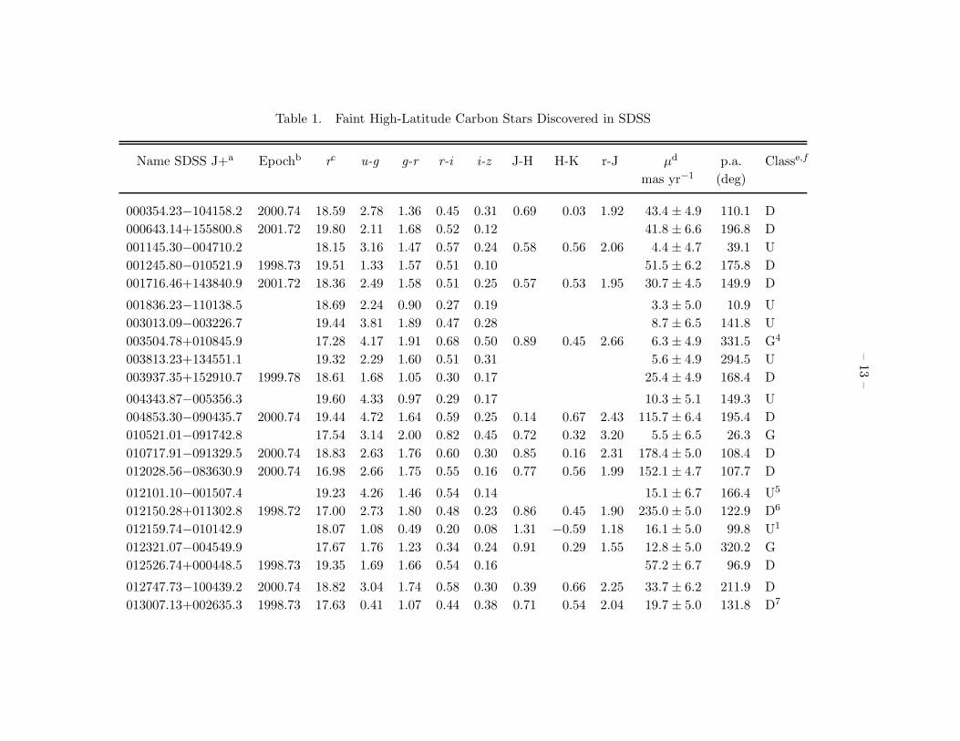
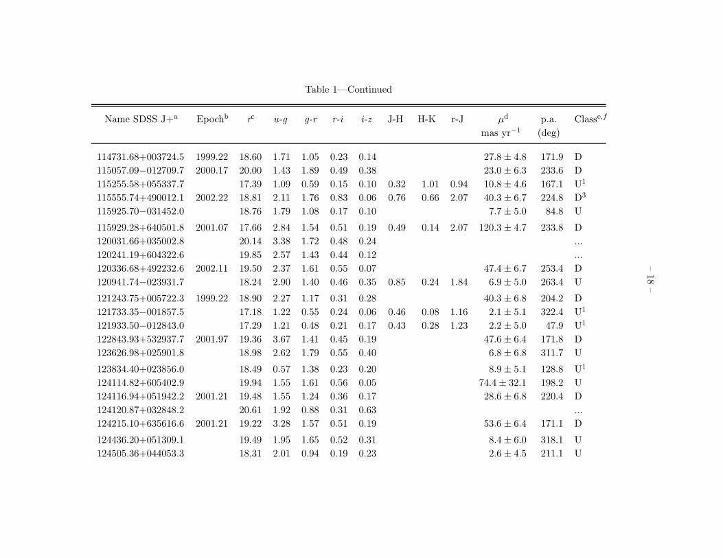
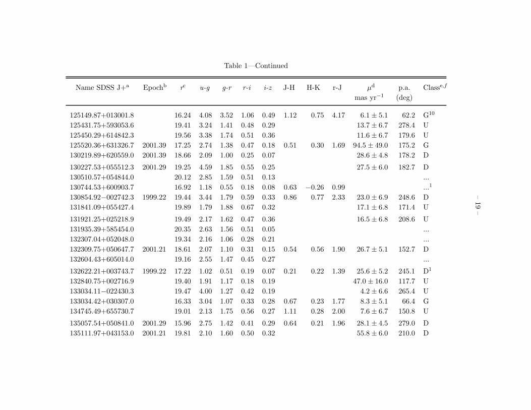
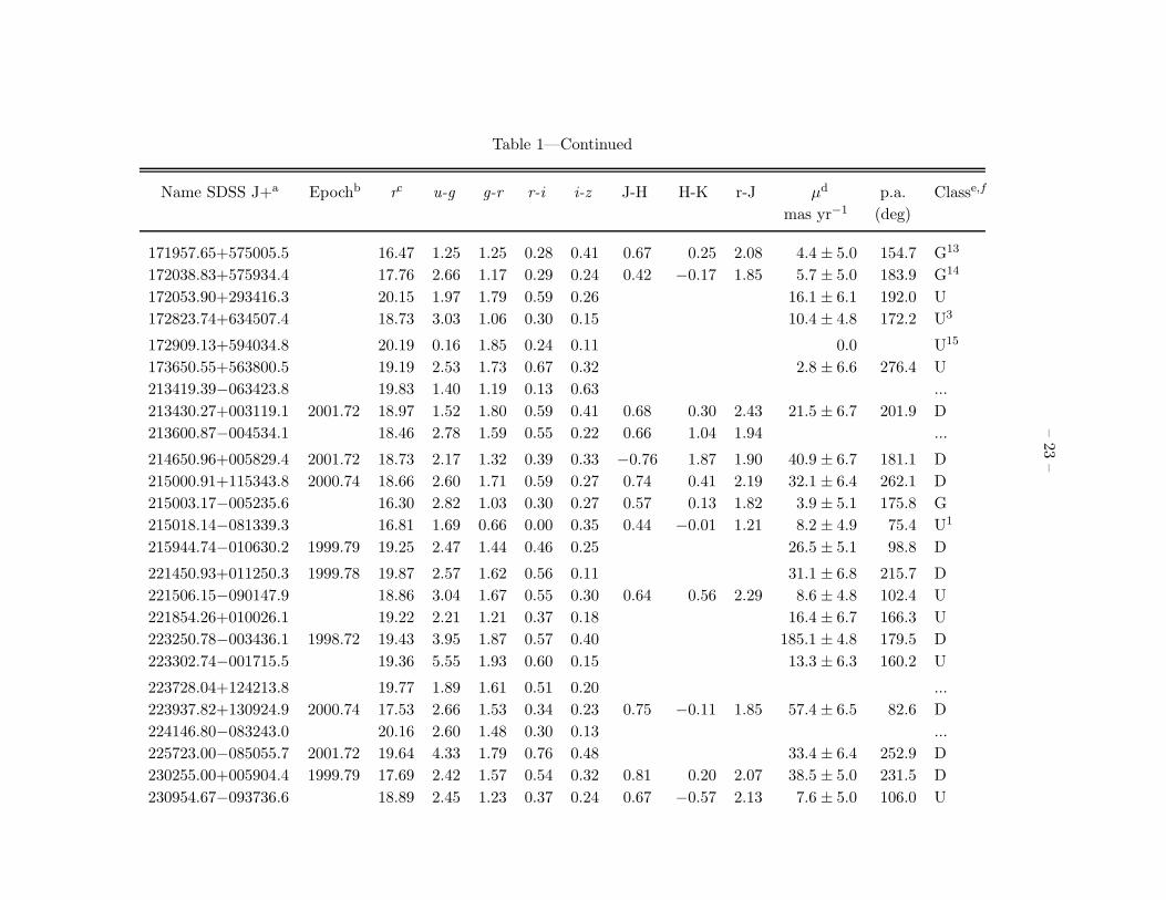
displayed in Paper I. The 251 objects are listed in Table 1, which provides astrometric (coordinates

and, when available, proper motions) and photometric (both Sloan and, when available, 2MASS

colors) data. We also note a luminosity class (giant or dwarf) based on the SDSS-derived proper

motions (see Paper I for details): all objects with 3σ detections of motion are considered dwarfs.

The spectra are qualitatively similar to those noted in Paper I, and we continue to see the broad

range of NaD strength (presumptively temperature) previously noted. However, the fraction of

objects with noticeable Balmer emission (6%) is only about half that seen in our initial sample.

A few special cases of extreme color are worthy of mention. In Paper I, no N-type stars were

detected by the selection software (the 2 objects shown there were found in an SDSS vs. 2MASS

comparison), although we noted that their extreme red colors should make them easier to find than

the R-type. Our expanded survey has resulted in the detection of one (but only one!) N-type star

- SDSS J125149.87+013001.8. A small fraction of the sample are exceptionally blue, and show

Balmer and Ca II absorption in addition to the C2 bands. These “F/G Carbon Stars”, discussed

elsewhere (Schroeder et al. 2002; Knapp et al. 2003), were initially found serendipitously. Searches

of the SDSS standard star sample, selected by colors optimized for metal-poor F-subdwarfs, then

added ∼ 20 more cases. This small fraction of very red or very blue objects, not found by our

nominal FHLC target selection software, stands as yet another warning of incompleteness in this

survey.

Figures 1-3 display color-color diagrams of the SDSS FHLCs, and define the location in the

1ftp.stsci.edu; cd pub/science/SDSS Carbon

– 4 –

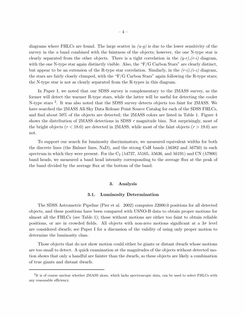
diagrams where FHLCs are found. The large scatter in (u-g) is due to the lower sensitivity of the

survey in the u band combined with the faintness of the objects; however, the one N-type star is

clearly separated from the other objects. There is a tight correlation in the (g-r),(r-i) diagram,

with the one N-type star again distinctly visible. Also, the “F/G Carbon Stars” are clearly distinct,

but appear to be an extension of the R-type star correlation. Similarly, in the (r-i),(i-z) diagram,

the stars are fairly closely clumped, with the “F/G Carbon Stars” again following the R-type stars;

the N-type star is not as clearly separated from the R-types in this diagram.

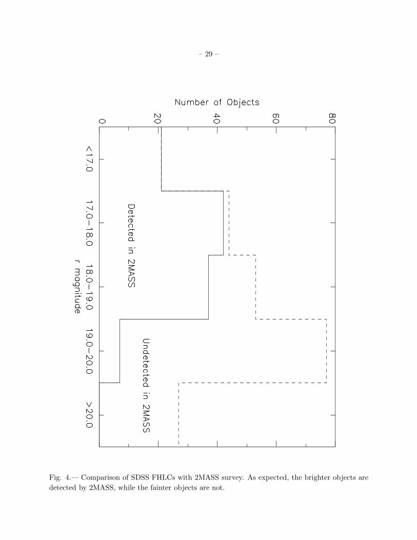
In Paper I, we noted that our SDSS survey is complementary to the 2MASS survey, as the

former will detect the warmer R-type stars, while the latter will be useful for detecting the cooler

N-type stars 2. It was also noted that the SDSS survey detects objects too faint for 2MASS. We

have searched the 2MASS All-Sky Data Release Point Source Catalog for each of the SDSS FHLCs,

and find about 50% of the objects are detected; the 2MASS colors are listed in Table 1. Figure 4

shows the distribution of 2MASS detections in SDSS r magnitude bins. Not surprisingly, most of

the bright objects (r < 18.0) are detected in 2MASS, while most of the faint objects (r > 19.0) are

not.

To support our search for luminosity discriminators, we measured equivalent widths for both

the discrete lines (the Balmer lines, NaD), and the strong CaH bands (λ6382 and λ6750) in each

spectrum in which they were present. For the C2 (λ4737, λ5165, λ5636, and λ6191) and CN (λ7900)

band heads, we measured a band head intensity corresponding to the average flux at the peak of

the band divided by the average flux at the bottom of the band.

3. Analysis

3.1. Luminosity Determination

The SDSS Astrometric Pipeline (Pier et al. 2002) computes J2000.0 positions for all detected

objects, and these positions have been compared with USNO-B data to obtain proper motions for

almost all the FHLCs (see Table 1); those without motions are either too faint to obtain reliable

positions, or are in crowded fields. All objects with non-zero motions significant at a 3σ level

are considered dwarfs; see Paper I for a discussion of the validity of using only proper motion to

determine the luminosity class.

Those objects that do not show motion could either be giants or distant dwarfs whose motions

are too small to detect. A quick examination at the magnitudes of the objects without detected mo-

tion shows that only a handful are fainter than the dwarfs, so these objects are likely a combination

of true giants and distant dwarfs.

2It is of course unclear whether 2MASS alone, which lacks spectroscopic data, can be used to select FHLCs with

any reasonable efficiency.

– 5 –

To determine which objects are close enough (if dwarfs) for a motion to be detectable, we

examined the distribution of observed motions, and find that most (over 90%) have proper motions

≥ 20 mas yr−1, which we take as our minimum detectable value. After converting the SDSS

magnitudes to V (Fukugita et al. 1996), and assuming MV = +10, we converted all proper

motions to a linear scale, and find that ∼ 90% of the objects have tangential velocities ≥ 50 km

s−1. Finally, we determined the V magnitude an object would have if it were at these limits (i.e.,

would be barely detectable), and find that Vmin = 18.6. This means that any object brighter than

this limit is likely a true giant, which is 32% (35) of the objects without observed motions; the

nature of the remaining objects must be considered uncertain. The occasional renegade dwarf may

of course by chance have a small tangential component to its motion. We exclude from this analysis

the “F/G Carbon Stars”, which are likely more luminous than the fiducial MV = +10, and label

them all of uncertain luminosity in Table 1, unless a positive detection of proper motion is present.

For the remaining 74 objects (excluding the 29 objects that had no proper motion data avail-

able), it is possible to make a statistical argument concerning the number that should be giants.

The faintest star in our sample has V=21.3, and it would need to have a tangential velocity of

175 km s−1 to be detectable. About one-third of the dwarfs have a motion above this limit, so

0.33 × 74 = 24 of the uncertain objects should be dwarfs with motions large enough to detect,

and hence the lack of detected motion implies they are true giants (although we don’t know which

ones). Thus, about half of the objects without detected motions are probably giants.

A different conclusion emerges, however, if a significant fraction of the sample is made of

disk dwarfs with space velocities smaller than velocities of halo stars. They will sometimes have

tangential velocities less than 50 km s−1, so some will contaminate the brighter stars that were called

giants above. They will all have tangential velocites less than 175 km s−1, so they may dominate the

fainter stars without significant motions, leaving fewer of the fainter uncertain objects as implied

giants than the 24 estimated above. In this case, significantly fewer than half of the objects without

detected motions would be giants. The population models made for Paper I indicated that disk

dwarfs were required to explain the stars with small radial velocities. A further analysis of the

population mix will be deferred to a future paper.

The total number of dwarfs in our survey (excluding the “F/G Carbon stars”) is 107, while

the total number of non-dwarfs (excluding the “F/G Carbon stars” and the 3 objects in the Draco

dwarf galaxy) is 117. Thus, at least 48% of the FHLCs are dwarfs, consistent with the estimate

of ≥ 50% of Paper I. If we assume half the uncertain objects are dwarfs, then at least 63% of the

FHLCs are dwarfs. The recent summary of known dC stars by Lowrance et al. (2003) lists 14

objects in total not due to SDSS. Thus, the homogeneous sample of SDSS stars in Table 1 that are

unambiguously dwarfs now constitutes 90% of all known dC stars.

In Paper I, we derived a surface density of 0.05 deg2, which was consistent with the value of

0.072±0.005 deg2 of Christlieb et al. (2001), derived from a bright, photographic sample. With the

same caveats about the completeness of our sample (see Paper I), we derived a surface density from

– 6 –

our expanded sample (224 objects in ∼3600 deg2) of 0.06 deg2 (again excluding the “F/G Carbon

stars” and the 3 Draco stars). It is clear that careful incompleteness corrections, not currently

available, will be needed to understand the true surface density of the faintest FHLCs.

4. Discussion

As previously noted, at least 50% the FHLCs are dwarfs. Therefore the development of a

simple observational luminosity discriminant is imperative if we are to, for example, use the giants

as halo velocity tracers. The fact that the dwarfs and giants differ in intrinsic luminosity by ∼ 10

mag gives hope that there would be such discriminants. In fact, several luminosity discriminants

have been proposed, although the small number of objects known to date has made it difficult

to assess the validity and range of applicability of these discriminants. With our large sample of

objects, an objective analysis of the proposed discriminants, as well as the possibility of uncovering

others, is now possible.

4.1. Previously proposed photometric luminosity discriminants

Numerous authors (e.g., Green et al. 1992; Joyce 1998; Totten et al. 2000; Lowrance

et al. 2003) have proposed near-IR colors as a luminosity discriminant, while MacConnell (2003)

showed a tight sequence for N-type stars for his survey objects in the (H-K), (J-H) diagram. While

we will discuss the luminosity aspect below, we present in Figure 5 the 2MASS color-color diagram

for all stars (∼ 100 stars) in our survey, in the carbon star catalog (|b| > 10◦; ∼ 300 stars) of Alk-

snis et al. (2001), and all previously reported FHLC dwarfs (11 stars), summarized by Lowrance

et al. (2003).

While the N-type stars continue to show the trend seen by MacConnell (2003), the R-type

stars are far more scattered, and the “F/G Carbon stars” appear to form a nice continuation of

the C stars sequence. The one N-type star in our survey fits nicely in with those from Alksnis

et al. (2001), while the one R-type star from Alksnis et al. (2001) at (H-K)=1.0 is classified as

R-N, so is likely an N-type; the R-type star at (H-K)=1.6 is the bright Mira variable RU Vir.

Although near-IR colors have been proposed as a luminosity discriminant, Wing & Jørgensen

(1996) and Jørgensen et al. (1998) argue on purely physical grounds that JHK colors alone should

not be an unambiguous indicator. Based on 4 objects from Paper I, we found that 2 objects

were consistent with the JHK discriminant, while 2 objects were not consistent. In Figure 6, we

show an enlargement of the near-IR color-color diagram, with just the SDSS stars, as well as the

previously known dwarfs, displayed. For (H-K) colors bluer than about 0.3, there is no separation

between giants and dwarfs. However, for redder colors, the bulk of the objects are dwarfs. For the

(somewhat arbitrary) line shown in the figure, 20 (74%) of the objects are dwarfs, 1 (4%) is a giant,

and 6 (22%) are uncertain; if only the confirmed giants and dwarfs are counted, then 95% of the

– 7 –

objects are dwarfs. A slight shift of the line to the blue (or red) does not significantly change the

giant to dwarf ratio. An examination of Figure 5 shows that most of the previously known dwarfs

do indeed appear to be offset from the bulk of the R-type stars from the Alksnis et al. (2001)

catalog, but with the addition of the SDSS FHLCs, it now appears that this discriminant can be

refined and confirmed.

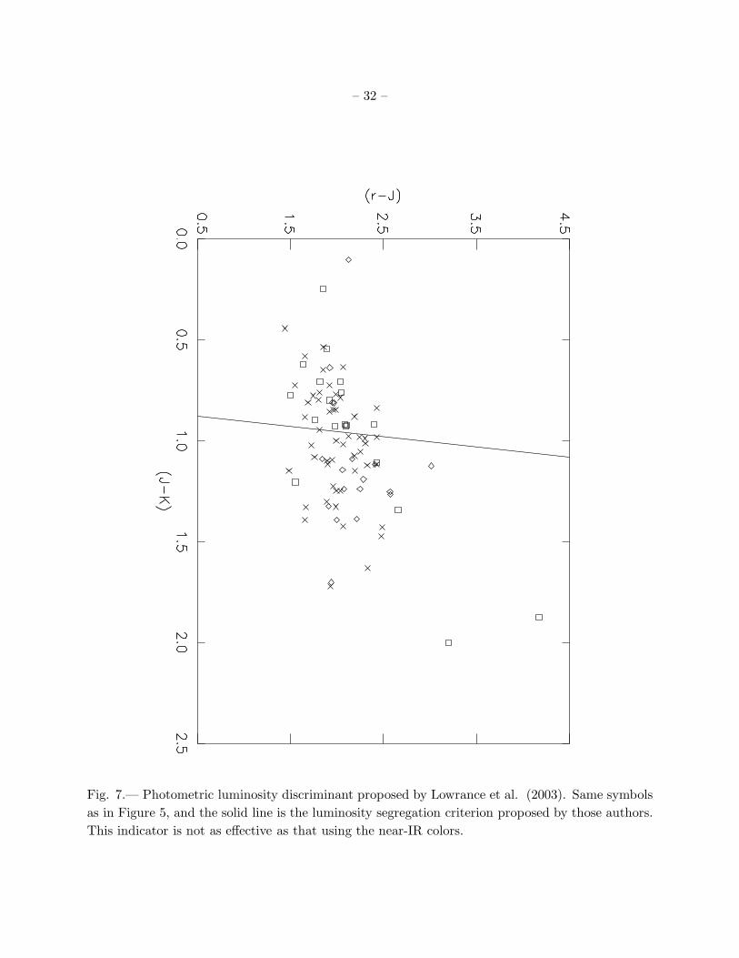
Lowrance et al. (2003) proposed that dwarfs and giants could be separated in the (J-K),

(R-J) diagram. While we do not have R magnitudes for our SDSS sample, the SDSS r band

should be a reasonable proxy to the Johnson R, so we have examined this discriminant with our

sample. Figure 7 shows that, as with the near-IR colors, this discriminant can identify dwarfs, but

is somewhat less effective (there are 5 giants in the dwarf region) than using only 2MASS colors.

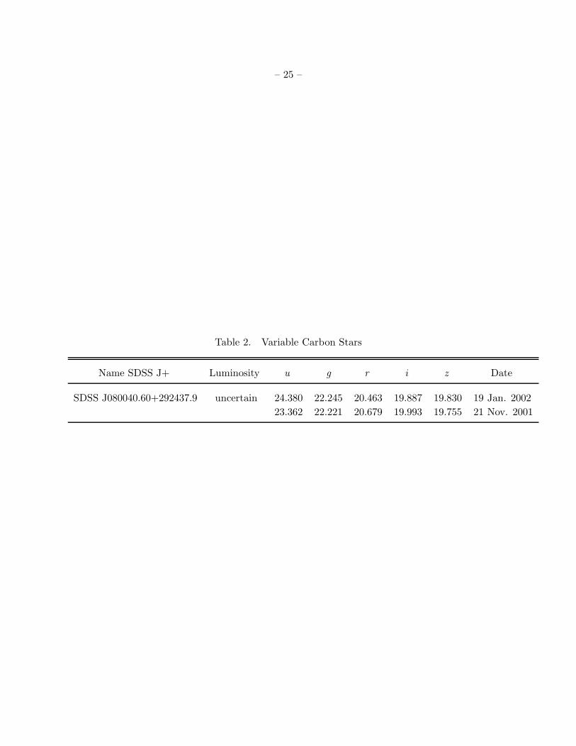
In Paper I, we commented that photometric variability may prove to be a simple luminosity

criterion, since only giants should show consistent, chaotic variations associated with mass loss;

absence of variability, however, does not imply the object is a dwarf. Many of the SDSS objects have

multiple photometric measurements in the imaging database, so we have performed a preliminary

check for variability. Given the faintness of many of the objects (particularly in u), we define an

object as variable if at least 2 of the g, r, and i magnitudes changed by at least 0.10 mag. With that

criteria, only 1 of the 49 FHLCs with multiple measurements is variable, and this object is listed in

Table 2. That object has an uncertain luminosity class, and thus is a strong candidate for a giant.

Note, however, that the object could be similar to the dC PG 0824+289 (Heber et al. 1993), which

shows variability due to heating effects from a hot companion, and so multiple measurements to

look for periodic variability would be interesting.

4.2. New photometric luminosity discriminants

In Figures 1-3, we plot the 3 SDSS color-color diagrams. An examination of those figures

shows that, while the “F/G Carbon stars” are clearly separated from the R-type stars, there is no

indication of a luminosity discriminant. We also investigated other color-color plots, none of which

presented any valid discriminant.

The model for a dwarf C star is that the C2 was deposited in a previous mass-transfer episode

from a companion that is now a faint white dwarf. In some cases (e.g., PG 0824+289 (Heber

et al. 1993); SBS 1517+5017 (Liebert et al. 1994)), the white dwarf is hot enough to be detectable

in the visible. However, in most cases, the white dwarf is too cool to be visible in the optical. We

examined those dwarfs in our sample that have the bluest u-g colors, to look for any spectroscopic

evidence of a white dwarf, but none was found. On the other hand, it may be possible to detect

the white dwarf in the ultraviolet, where the C star is faint and the contrast may be optimized.

To determine how faint (i.e., cool) the white dwarf would typically have to be to be undetected

either spectroscopically or photometrically, we selected one blue and one red giant FHLC from our

sample, and added a blackbody and/or real white dwarf spectrum of various temperatures. We

– 8 –

find that a 10,000 K blackbody is barely detectable in the red giant, while an 11,000 K blackbody

is barely detectable in the blue giant. However, in the satellite ultraviolet, these cool white dwarfs

could be detectable (e.g., with the ACS SBC camera on HST). Therefore, UV colors may in fact

be a useful photometric luminosity discriminant.

4.3. Previously proposed spectroscopic luminosity discriminants

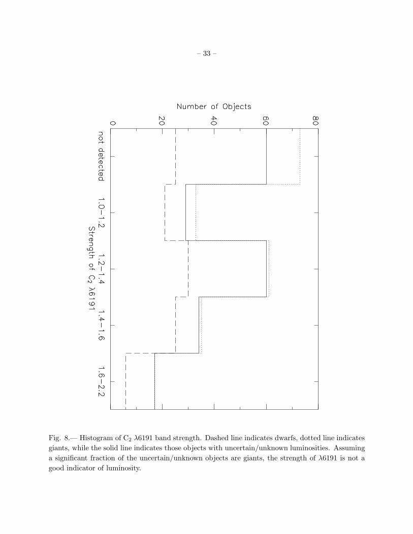
Numerous spectroscopic luminosity discriminants have been previously proposed. Green et al. (1992)

proposed that the appearance of a strong C2 band head at λ6191 indicated the object was a dwarf,

while Margon et al. (2002) suggested the feature was both temperature and luminosity dependent.

However, both studies noted that while the absence of λ6191 could not be used to firmly classify

the object as a giant, the presence of λ6191 was a good indicator that the object is a dwarf. In

Figure 8 we show a histogram of the strength of λ6191, which demonstrates that this feature is in

fact probably not a good luminosity discriminant. When λ6191 is weak (1.0-1.4), about 50% of

the objects are confirmed dwarfs, while at its strongest (> 1.6) about a third of the objects are

confirmed dwarfs. Only in the 1.4-1.6 bin do the dwarfs dominate (70%). In total, 50% of the

objects with λ6191 are confirmed dwarfs, so this feature can no longer be considered a luminosity

discriminant.

In Paper I we suggested that the presence of Hα emission could be an indicator that the

object is a giant, since dwarfs are unlikely to process active chromospheres or undergo active

mass loss. However, a contrary case (PG 0824+289) was noted, where heating of the dwarf by a

hot DA companion caused the emission. In that case, the white dwarf was visible in the optical

spectrum, so Hα emission in dCs where there is no indication of a hot white dwarf could still be

a luminosity discriminant. Of the 14 objects in our sample with Hα emission, 3 are giants, 3 are

dwarfs, and the remaining 8 have are uncertain luminosity. Thus, the use of Hα emission as a

luminosity discriminant is speculative. The dCs with Hα emission are rare, and thus should be

further observed.

The bands of CaH at λλ6382, 6750 are normally strong only in K and M dwarfs (e.g., Kilk-

patrick et al. 1991), which led us to suggest in Paper I that the presence of these features was a

luminosity indicator in FHLCs. In Figure 9 we show plot of the equivalent width of λ6750 versus

that of NaD. While it is true that there are no giants whose spectra show CaH, there are 10 objects

(out of 16 total) that have an uncertain luminosity. So, while promising, this discriminant must

still be consider unproven.

It is interesting to note that sharp turn-on of the CaH feature at Wλ(NaD) = 10 A, although

there are two objects (one with weaker NaD (hotter) which shows CaH, one with stronger NaD

(cooler) that does not) that are exceptions. To estimate the temperature of this turn-on point,

the temperature index (Cohen 1979) of every star that showed NaD was measured, and a fit of

NaD as a function of Temperature Index was made. The Temperature index was converted to a

– 9 –

temperature (Yamashita 1967), with the result that the CaH turn-on occurs at T=2900 K.

Green et al. (1992) suggested that dC’s have strong λ6191 band heads given their relatively

weak CN band strength. In Figure 10, we plot the strength of λ6191 versus the strength of the CN

band at λ7900. Unfortunately, there are so few confirmed giants which show CN that a definitive

statement about this criterion is not possible. However, given the range of λ6191 strengths seen for

the dwarfs alone, this discriminant can be considered doubtful. On the other hand, the strength

of the CN band alone, particularly at the weakest and stronger levels, may be a discriminant (see

below).

4.4. New spectroscopic luminosity discriminants

With our large sample of FHLCs, we have searched for possible new spectroscopic discrimi-

nants. Christlieb et al. (2001) found a correlation between the strengths of the C2 bands at λ5165

and λ4737, which they used for detection of carbon stars. Our data also shows this correlation, but

there is no separation between dwarfs, giants, and the stars of uncertain luminosity. In a similar

vein, we show, in Figure 11, the equivalent relation for the strongest C2 bands. Again, there is a

correlation, but C2 band strength does not appear to be a luminosity discriminant.

As previously noted, the strength of the CN band at λ7900 may be a luminosity indicator. In

Figure 12, we plot a histogram of the strength of this feature. As can be seen, all objects with band

strengths greater than 1.6 are either giants (6) or of uncertain luminosity (1; the object with the

strongest CN). Similarly, most of the objects with weak CN are dwarfs (19); there are 2 giants and

1 object of uncertain luminosity. Thus, extremely strong CN seems to imply a giant luminosity,

while extremely weak (but present) CN implies a dwarf luminosity.

5. Summary

We have increased our SDSS survey of faint high-latitude carbon stars to include 251 objects,

at least 50% of which are dwarfs. Although giant and dwarf carbon stars differ in luminosity

by 10 mag, the spectra (at the SDSS spectral resolution of 103) are extremely similar. We have

used our expanded sample to search for photometric and spectroscopic discriminants, including an

examination of those previously proposed.

We find that SDSS colors and the strength of the C2 band head at λ6191 are not good lu-

minosity discriminants, while the presence of Hα emission as a discriminant is speculative. The

suggestion from Paper I that the CaH bands at λλ6382, 6750 indicate that the object is a dwarf

must also still be considered unproven.

The strength of the CN band at λ7900, when it is extremely strong or extremely weak, appears

to be a good luminosity discriminant. However, it is of limited use, as almost half the objects do not

– 10 –

show this band. For the redder objects, the use of JHK colors appears to allow the identification of

dwarfs. Another possible discriminant is ultraviolet colors, where the presumed white dwarf (which

transferred its carbon to the now dC star) may be detectable.

We thank J. MacConnell for helpful comments. This publication makes use of data products

from the Two Micron All Sky Survey, which is a joint project of the University of Massachusetts

and the Infrared Processing and Analysis Center/California Institute of Technology, funded by

NASA and the NSF. This research has also made use of the SIMBAD database, operated at

CDS, Strasbourg, France, and the NASA/IPAC Infrared Science Archive, which is operated by the

Jet Propulsion Laboratory, California Institute of Technology, under contract with the National

Aeronautics and Space Administration.

Funding for the creation and distribution of the SDSS Archive has been provided by the

Alfred P. Sloan Foundation, the Participating Institutions, the National Aeronautics and Space

Administration, the National Science Foundation, the US Department of Energy, the Japanese

Monbukagakusho, and the Max Planck Society. The SDSS Web site is http://www.sdss.org/.

The SDSS is managed by the Astrophysical Research Consortium (ARC) for the Participating

Institutions. The Participating Institutions are The University of Chicago, Fermilab, the Institute

for Advanced Study, the Japan Participation Group, The Johns Hopkins University, Los Alamos

National Laboratory, the Max-Planck-Institute for Astronomy (MPIA), the Max-Planck-Institute

for Astrophysics (MPA), New Mexico State University, University of Pittsburgh, Princeton Uni-

versity, the US Naval Observatory, and the University of Washington.

– 11 –

REFERENCES

Abazajian, K., Adelman, J., Agueros, M. et al. 2003, AJ, 126, 2081

Alksnis, A., Balklavs, A., Dzervitis, U., Eglitis, I., Paupers, O., & Pundure, I. 2001, Baltic Astron.,

10, 1

Bothun, G., Elias, J. H., MacAlpine, G., Matthews, K., Mould, J. R., Neugebauer, G., & Reid, I.

N. 1991, AJ, 101, 2220

Christlieb, N., Green, P. J., Wisotzki, L., & Reimers, D. 2001, A&A, 375, 366

Cohen, M. 1979, MNRAS, 186, 837

Duner, N.-C. 1884, Sur les etoiles a spectres de la troisieme classe (Stockholm: Norstedt)

Fukugita, M., Ichikawa, T., Gunn, J. E., Doi, M., Shimasaku, K., & Schneider, D. P. 1996, AJ,

111, 1748

Grebel, E. 2004, private communication

Green, P. J., Margon, B., Anderson, S. F., & MacConnell, D. J. 1992, ApJ, 400, 659

Gunn, J. E., Carr, M. A., Rockosi, C. M., Sekiguchi, M. et al. 1998, AJ, 116, 3040

Heber, U., Bade, N., Jordan, S., & Voges, W. 1993, A&A, 267, L31

Hendon, A. A. & Stone, R. C. 1998, AJ, 115, 296

Hogg, D. W., Schlegel, D. J., Finkbeiner, D. P., & Gunn, J. E. 2001, AJ, 122, 2129

Jørgensen, U. G., Borysow, A., & Hofner, S. 1998, in ASP Conf. Ser. 138, 1997 Pacific Rim

Conference on Stellar Atmospheres, ed. K. L. Chan, K. S. Cheng, & H. P. Singh (San

Francisco : ASP), 157

Joyce, R. R. 1998, AJ, 115, 2059

Kirkpatrick, J. D., Henry, T. J., & McCarthy, D. W. 1991, ApJS, 77, 417

Knapp, G. R. et al. 2003, in preparation

Krisciunas, K., Margon, B., & Szkody, P. 1998, PASP, 110, 1342

Liebert, J., Schmidt, G. D., Lesser, M., Stepanian, J. A., Lipovetsky, V. A., Chaffee, F. H., Foltz,

C. B., & Bergeron, P. 1994, ApJ, 421, 733

Lowrance, P. J., Kirkpatrick, J. D., Reid, I. N., Cruz, K. L., & Liebert, J. 2003, ApJ, 584, L95

– 12 –

Lupton, R., Gunn, J. E., Ivezic, Z., Gnapp, J. R., Kent, S., & Yasuda, N. 2001, in ASP Conf.

Ser. 238, Astronomical Data Analysis Software and Systems X, ed. F. R. Harnden, Jr., A.

Primini, & H. E. Payne (San Francisco : ASP), 269

MacConnell, D. J. 2003, PASP, 115, 351

Margon, B. et al. 2002, AJ, 124, 1651 (Paper I)

Mould, J. R., Schneider, D. P., Gordon, G. A., Aaronson, M., & Liebert, J. W. 1985, PASP, 97,

130

Pier, J. R., Munn, J. A., Hindsley, R. B., Hennessy, G. S., Kent, S. M., Lupton, R. H., & Ivezic,

Z. 2002, AJ, 125, 1559

Schroeder, J. et al. 2002, BAAS, 34, 1126

Smith, J. A., Tucker, D. L., Kent, S. M., et al. 2002, AJ, 123, 2121

Stoughton, C. et al. 2002, AJ, 123, 485 (Early Data Release)

Totten, E. J. & Irwin, M. J. 1998, MNRAS, 294, 1

Totten, E. J., Irwin, M. J., & Whitelock, P. A. 2000, MNRAS, 314, 630

Wing, R. F. & Jørgensen, U. G. 1996, BAAS, 28, 1382

Yamashita, Y. 1967, Pub. Dom. Astrophys. Obs., XIII, 67

York, D. G., Adelman, J., Anderson, J. E., et al. 2000, AJ, 120, 1579

This preprint was prepared with the AAS LATEX macros v5.2.

–13

–

Table 1. Faint High-Latitude Carbon Stars Discovered in SDSS

Name SDSS J+a Epochb rc u-g g-r r-i i-z J-H H-K r-J µd p.a. Classe,f

mas yr−1 (deg)

000354.23−104158.2 2000.74 18.59 2.78 1.36 0.45 0.31 0.69 0.03 1.92 43.4 ± 4.9 110.1 D

000643.14+155800.8 2001.72 19.80 2.11 1.68 0.52 0.12 41.8 ± 6.6 196.8 D

001145.30−004710.2 18.15 3.16 1.47 0.57 0.24 0.58 0.56 2.06 4.4 ± 4.7 39.1 U

001245.80−010521.9 1998.73 19.51 1.33 1.57 0.51 0.10 51.5 ± 6.2 175.8 D

001716.46+143840.9 2001.72 18.36 2.49 1.58 0.51 0.25 0.57 0.53 1.95 30.7 ± 4.5 149.9 D

001836.23−110138.5 18.69 2.24 0.90 0.27 0.19 3.3 ± 5.0 10.9 U

003013.09−003226.7 19.44 3.81 1.89 0.47 0.28 8.7 ± 6.5 141.8 U

003504.78+010845.9 17.28 4.17 1.91 0.68 0.50 0.89 0.45 2.66 6.3 ± 4.9 331.5 G4

003813.23+134551.1 19.32 2.29 1.60 0.51 0.31 5.6 ± 4.9 294.5 U

003937.35+152910.7 1999.78 18.61 1.68 1.05 0.30 0.17 25.4 ± 4.9 168.4 D

004343.87−005356.3 19.60 4.33 0.97 0.29 0.17 10.3 ± 5.1 149.3 U

004853.30−090435.7 2000.74 19.44 4.72 1.64 0.59 0.25 0.14 0.67 2.43 115.7 ± 6.4 195.4 D

010521.01−091742.8 17.54 3.14 2.00 0.82 0.45 0.72 0.32 3.20 5.5 ± 6.5 26.3 G

010717.91−091329.5 2000.74 18.83 2.63 1.76 0.60 0.30 0.85 0.16 2.31 178.4 ± 5.0 108.4 D

012028.56−083630.9 2000.74 16.98 2.66 1.75 0.55 0.16 0.77 0.56 1.99 152.1 ± 4.7 107.7 D

012101.10−001507.4 19.23 4.26 1.46 0.54 0.14 15.1 ± 6.7 166.4 U5

012150.28+011302.8 1998.72 17.00 2.73 1.80 0.48 0.23 0.86 0.45 1.90 235.0 ± 5.0 122.9 D6

012159.74−010142.9 18.07 1.08 0.49 0.20 0.08 1.31 −0.59 1.18 16.1 ± 5.0 99.8 U1

012321.07−004549.9 17.67 1.76 1.23 0.34 0.24 0.91 0.29 1.55 12.8 ± 5.0 320.2 G

012526.74+000448.5 1998.73 19.35 1.69 1.66 0.54 0.16 57.2 ± 6.7 96.9 D

012747.73−100439.2 2000.74 18.82 3.04 1.74 0.58 0.30 0.39 0.66 2.25 33.7 ± 6.2 211.9 D

013007.13+002635.3 1998.73 17.63 0.41 1.07 0.44 0.38 0.71 0.54 2.04 19.7 ± 5.0 131.8 D7

–14

–

Table 1—Continued

Name SDSS J+a Epochb rc u-g g-r r-i i-z J-H H-K r-J µd p.a. Classe,f

mas yr−1 (deg)

013148.46+004230.7 1998.72 19.05 1.85 1.05 0.17 0.19 19.1 ± 5.0 78.1 D

013249.99+000300.4 20.52 1.36 1.21 0.34 0.47 ...

014140.31−100355.1 19.60 3.99 1.76 0.55 0.33 19.2 ± 6.6 152.1 U

015025.80−001315.1 17.62 1.09 0.42 0.09 0.05 0.30 −0.31 1.10 6.4 ± 4.8 143.1 U1

015232.31−004932.6 1998.72 18.15 2.69 1.68 0.48 0.26 0.66 0.13 2.04 14.9 ± 4.8 128.9 D

020716.86+133034.7 19.49 2.04 1.02 0.28 0.28 8.7 ± 4.6 176.2 U

021119.82+003201.5 19.73 3.30 1.65 0.56 0.28 6.4 ± 6.6 249.2 U

023208.60+003639.3 1998.73 19.46 2.09 1.59 0.56 0.28 21.7 ± 6.8 19.2 D

025634.62−084853.8 1999.79 19.47 1.94 1.11 0.27 0.17 35.2 ± 6.8 137.4 D

030837.07+005157.1 20.63 1.92 1.89 0.44 0.41 ...

032955.54−000354.0 17.96 1.16 0.53 0.19 0.08 0.27 0.56 1.18 6.5 ± 4.8 141.7 U1

033704.05−001603.0 18.67 2.48 1.92 0.71 0.30 0.79 0.33 2.41 12.0 ± 5.0 116.1 U

034705.41−063323.9 2000.74 16.17 1.00 0.39 0.17 0.04 0.36 −0.02 1.01 24.0 ± 5.1 171.4 D1

073621.29+390725.2 2000.32 18.43 3.21 1.52 0.46 0.16 0.68 0.65 1.67 55.6 ± 4.7 230.1 D

073805.73+274148.8 2001.97 18.46 2.49 1.57 0.55 0.21 0.78 0.10 2.19 19.1 ± 6.3 159.4 D

074109.31+243603.0 19.95 2.17 1.51 0.53 0.04 ...

074638.21+400403.5 19.52 3.08 1.68 0.51 0.21 ...

074710.84+251619.6 18.12 1.06 0.42 0.15 0.10 10.3 ± 4.5 177.5 U1

075116.37+391201.4 17.61 3.47 1.60 0.58 0.43 0.81 0.30 2.43 3.9 ± 4.7 168.9 G

075228.63+280547.5 2002.02 20.09 1.55 1.63 0.49 0.10 34.4 ± 6.6 191.2 D

075953.64+434021.1 19.48 3.64 1.91 0.63 0.15 3.9 ± 6.6 324.3 U

080040.60+292437.9 20.46 2.13 1.78 0.58 0.06 ...8

–15

–

Table 1—Continued

Name SDSS J+a Epochb rc u-g g-r r-i i-z J-H H-K r-J µd p.a. Classe,f

mas yr−1 (deg)

080046.72+364107.1 17.37 1.06 0.41 0.13 0.08 0.63 −0.01 1.04 3.5 ± 4.8 220.4 U1

080156.39+395043.8 18.46 4.16 1.65 0.54 0.26 0.59 0.50 2.16 2.0 ± 5.0 125.7 U

080806.06+293634.1 18.34 3.22 1.18 0.33 0.35 0.71 0.10 1.95 6.3 ± 5.0 6.6 U

080908.15+360129.0 18.89 0.32 0.44 0.25 0.10 6.1 ± 4.8 192.4 U

082127.90+333037.2 19.46 2.62 1.21 0.33 0.22 11.0 ± 21.7 256.9 U

082251.41+461232.3 2000.26 17.23 2.79 1.40 0.47 0.23 0.82 0.20 1.73 27.1 ± 5.0 221.3 D

082626.76+470911.7 2000.26 17.77 2.80 1.46 0.48 0.31 0.60 0.17 1.99 39.6 ± 4.8 148.9 D

084130.12+435136.7 2001.15 19.45 2.52 1.52 0.48 0.23 33.6 ± 6.3 354.7 D

084720.16+003340.4 20.73 1.14 1.92 0.56 0.21 ...

085212.77+383721.9 2002.02 19.93 3.10 1.69 0.51 0.18 51.8 ± 6.4 204.2 D

085853.28+012243.5 2000.34 18.31 2.46 1.99 0.67 0.36 0.71 0.72 2.49 32.1 ± 4.7 124.3 D

090011.35−003606.5 1999.22 18.44 3.27 1.48 0.47 0.26 53.8 ± 6.4 168.4 D

090208.05+435503.8 17.43 1.19 0.47 0.14 0.06 4.5 ± 4.8 135.2 U1

091007.61+521612.4 17.01 2.94 1.63 0.54 0.27 0.72 0.20 2.09 12.6 ± 4.8 177.4 G

091019.21+041211.6 19.05 3.42 1.50 0.54 0.38 12.2 ± 6.0 279.3 U

091335.63+492444.7 19.83 2.12 1.60 0.49 0.25 8.0 ± 6.5 212.6 U

091336.99+034839.1 2001.14 18.86 2.34 1.27 0.38 0.23 35.4 ± 6.0 150.0 D

092508.21+010545.4 17.94 2.66 1.29 0.44 0.32 0.49 0.27 2.05 6.3 ± 4.8 190.6 G

092545.46+424929.0 2002.02 17.51 1.11 0.43 0.11 0.04 0.25 −0.26 0.98 20.5 ± 4.8 156.6 D1

093057.12+033453.6 19.23 2.41 1.60 0.55 0.35 16.5 ± 6.1 349.8 U

093203.67+002753.8 20.40 1.00 1.66 0.45 0.10 ...

093741.12+470836.2 2001.96 18.6g 0.20 0.93 61.5 ± 4.8 199.9 D

094209.94+535719.2 16.49 2.61 1.44 0.53 0.30 0.72 0.21 1.98 7.2 ± 4.8 352.4 G

–16

–

Table 1—Continued

Name SDSS J+a Epochb rc u-g g-r r-i i-z J-H H-K r-J µd p.a. Classe,f

mas yr−1 (deg)

094318.73+032743.7 2001.14 18.11 2.70 1.38 0.49 0.13 0.54 0.04 1.66 34.9 ± 4.5 229.4 D

094511.57+503214.5 2002.02 18.86 5.21 1.32 0.40 0.22 15.4 ± 4.8 202.7 D3

094858.68+583020.5 2000.26 18.77 2.55 1.15 0.33 0.22 26.9 ± 4.7 163.2 D

095005.09+584123.8 2000.26 17.03 2.93 1.43 0.47 0.18 0.67 0.41 1.76 102.9 ± 4.7 162.5 D

095516.39+012129.8 18.36 2.85 1.60 0.53 0.26 0.86 −0.05 1.97 7.4 ± 4.9 100.9 U

100132.62+020402.7 19.41 3.84 1.68 0.61 0.20 10.9 ± 6.3 237.9 U

100432.45+004337.7 1999.22 19.99 1.78 1.71 0.56 0.19 32.1 ± 6.4 169.1 D

100627.47+462117.4 17.52 0.96 0.44 0.15 0.10 0.26 0.19 1.31 10.4 ± 5.0 164.5 U1

100638.20+473039.5 2001.97 19.96 1.88 1.65 0.54 0.27 37.2 ± 6.7 161.4 D

100812.04+012657.2 2000.34 20.17 3.60 1.73 0.51 0.15 425.2 ± 6.3 190.7 D

100913.95+514924.6 2002.02 18.55 2.66 1.44 0.45 0.16 0.64 0.15 1.80 75.8 ± 5.0 217.4 D

100958.70+010313.2 1999.22 17.07 2.26 1.03 0.27 0.14 0.41 0.03 1.44 35.9 ± 4.8 171.8 D

101007.11+031444.1 18.96 1.97 1.78 0.63 0.40 1.03 0.21 2.25 8.9 ± 6.6 129.9 U

101210.81+465249.1 2002.04 18.36 2.76 1.39 0.46 0.29 1.01 0.39 1.66 22.6 ± 6.6 218.5 D

101422.75+464737.3 19.77 2.34 1.52 0.52 0.09 18.5 ± 6.6 149.1 U

102239.58+622344.7 19.88 2.24 1.79 0.37 0.34 11.2 ± 6.4 250.8 U

102433.76+562855.1 19.51 2.37 1.78 0.56 0.20 3.5 ± 6.5 308.6 U

102908.38+591853.8 18.93 1.91 1.36 0.46 0.18 10.9 ± 4.9 175.0 U

102941.07+020613.1 19.48 2.62 1.75 0.58 0.26 10.7 ± 6.2 169.4 U

103758.57+612559.3 2000.26 18.08 1.00 0.36 0.19 −0.01 17.9 ± 4.9 156.8 D1

104138.55+643219.8 18.48 2.45 1.89 0.75 0.42 0.68 0.58 2.58 3.1 ± 6.4 208.4 U

104316.17+573755.7 19.96 1.54 1.55 0.54 0.11 ...

–17

–

Table 1—Continued

Name SDSS J+a Epochb rc u-g g-r r-i i-z J-H H-K r-J µd p.a. Classe,f

mas yr−1 (deg)

105629.95+012208.8 17.52 1.09 0.54 0.18 0.05 0.09 −0.77 1.32 6.6 ± 5.0 180.1 U1

105806.72+032514.7 18.40 2.77 1.28 0.37 0.23 0.59 0.04 1.93 4.0 ± 6.3 160.5 U

110558.06+510942.9 2001.97 18.91 3.76 1.88 0.54 0.15 0.99 0.73 1.93 51.2 ± 6.7 204.3 D

110607.96+495055.0 2001.97 18.82 2.89 1.56 0.55 0.14 65.0 ± 6.4 200.0 D

111833.84+563958.1 2001.89 16.65 0.88 0.35 0.15 0.02 0.27 0.18 0.98 19.8 ± 4.8 222.0 D1

112034.87+555937.2 2001.97 16.15 2.75 1.31 0.43 0.15 0.64 0.14 1.74 95.3 ± 4.5 200.9 D

112417.34+054921.3 20.30 4.73 1.19 0.31 0.24 23.4 ± 30.7 359.6 U

112631.31+053705.3 20.26 3.42 1.79 0.55 0.23 15.4 ± 6.7 166.7 U

112650.77+645646.0 19.09 3.15 1.39 0.45 0.25 11.2 ± 4.8 198.7 U

112654.85+645155.8 20.30 2.27 1.78 0.57 0.09 6.4 ± 6.6 225.9 U

112746.45+041502.5 2001.14 18.92 2.99 1.54 0.49 0.29 51.9 ± 5.0 148.7 D

112752.79+515815.2 2001.97 17.68 2.89 1.21 0.38 0.24 0.61 0.27 1.66 29.1 ± 4.5 169.9 D

112801.68+004034.7 18.81 2.46 1.41 0.38 0.23 19.0 ± 6.8 171.0 U9

112836.57+011331.2 17.23 1.03 0.43 0.17 0.09 0.60 0.01 1.05 2.2 ± 5.2 288.5 U1

112900.75+510742.0 2001.97 20.14 1.81 1.44 0.48 0.04 23.0 ± 6.0 167.2 D

112950.38+003344.9 1999.22 18.28 2.27 1.40 0.41 0.33 0.77 0.17 1.81 39.6 ± 6.8 234.2 D

113040.49+525039.2 17.34 1.14 0.45 0.13 0.03 0.28 −0.36 1.01 6.4 ± 4.5 266.8 U1

113720.88−012515.7 2000.17 19.14 3.34 1.28 0.37 0.23 29.6 ± 6.2 230.5 D

113931.62+050231.2 19.59 2.03 1.69 0.56 0.39 17.5 ± 6.3 164.8 U

114125.85+010504.3 17.29 2.12 0.89 0.15 0.29 0.42 0.35 1.50 3.9 ± 4.8 85.7 G

114355.88+625924.7 2001.38 19.41 1.62 1.55 0.51 0.32 35.2 ± 6.5 167.6 D

114442.36+043641.9 2001.29 19.17 2.31 1.39 0.31 0.29 35.0 ± 6.2 275.5 D

–18

–

Table 1—Continued

Name SDSS J+a Epochb rc u-g g-r r-i i-z J-H H-K r-J µd p.a. Classe,f

mas yr−1 (deg)

114731.68+003724.5 1999.22 18.60 1.71 1.05 0.23 0.14 27.8 ± 4.8 171.9 D

115057.09−012709.7 2000.17 20.00 1.43 1.89 0.49 0.38 23.0 ± 6.3 233.6 D

115255.58+055337.7 17.39 1.09 0.59 0.15 0.10 0.32 1.01 0.94 10.8 ± 4.6 167.1 U1

115555.74+490012.1 2002.22 18.81 2.11 1.76 0.83 0.06 0.76 0.66 2.07 40.3 ± 6.7 224.8 D3

115925.70−031452.0 18.76 1.79 1.08 0.17 0.10 7.7 ± 5.0 84.8 U

115929.28+640501.8 2001.07 17.66 2.84 1.54 0.51 0.19 0.49 0.14 2.07 120.3 ± 4.7 233.8 D

120031.66+035002.8 20.14 3.38 1.72 0.48 0.24 ...

120241.19+604322.6 19.85 2.57 1.43 0.44 0.12 ...

120336.68+492232.6 2002.11 19.50 2.37 1.61 0.55 0.07 47.4 ± 6.7 253.4 D

120941.74−023931.7 18.24 2.90 1.40 0.46 0.35 0.85 0.24 1.84 6.9 ± 5.0 263.4 U

121243.75+005722.3 1999.22 18.90 2.27 1.17 0.31 0.28 40.3 ± 6.8 204.2 D

121733.35−001857.5 17.18 1.22 0.55 0.24 0.06 0.46 0.08 1.16 2.1 ± 5.1 322.4 U1

121933.50−012843.0 17.29 1.21 0.48 0.21 0.17 0.43 0.28 1.23 2.2 ± 5.0 47.9 U1

122843.93+532937.7 2001.97 19.36 3.67 1.41 0.45 0.19 47.6 ± 6.4 171.8 D

123626.98+025901.8 18.98 2.62 1.79 0.55 0.40 6.8 ± 6.8 311.7 U

123834.40+023856.0 18.49 0.57 1.38 0.23 0.20 8.9 ± 5.1 128.8 U1

124114.82+605402.9 19.94 1.55 1.61 0.56 0.05 74.4 ± 32.1 198.2 U

124116.94+051942.2 2001.21 19.48 1.55 1.24 0.36 0.17 28.6 ± 6.8 220.4 D

124120.87+032848.2 20.61 1.92 0.88 0.31 0.63 ...

124215.10+635616.6 2001.21 19.22 3.28 1.57 0.51 0.19 53.6 ± 6.4 171.1 D

124436.20+051309.1 19.49 1.95 1.65 0.52 0.31 8.4 ± 6.0 318.1 U

124505.36+044053.3 18.31 2.01 0.94 0.19 0.23 2.6 ± 4.5 211.1 U

–19

–

Table 1—Continued

Name SDSS J+a Epochb rc u-g g-r r-i i-z J-H H-K r-J µd p.a. Classe,f

mas yr−1 (deg)

125149.87+013001.8 16.24 4.08 3.52 1.06 0.49 1.12 0.75 4.17 6.1 ± 5.1 62.2 G10

125431.75+593053.6 19.41 3.24 1.41 0.48 0.29 13.7 ± 6.7 278.4 U

125450.29+614842.3 19.56 3.38 1.74 0.51 0.36 11.6 ± 6.7 179.6 U

125520.36+631326.7 2001.39 17.25 2.74 1.38 0.47 0.18 0.51 0.30 1.69 94.5 ± 49.0 175.2 G

130219.89+620559.0 2001.39 18.66 2.09 1.00 0.25 0.07 28.6 ± 4.8 178.2 D

130227.53+055512.3 2001.29 19.25 4.59 1.85 0.55 0.25 27.5 ± 6.0 182.7 D

130510.57+054844.0 20.12 2.85 1.59 0.51 0.13 ...

130744.53+600903.7 16.92 1.18 0.55 0.18 0.08 0.63 −0.26 0.99 ...1

130854.92−002742.3 1999.22 19.44 3.44 1.79 0.59 0.33 0.86 0.77 2.33 23.0 ± 6.9 248.6 D

131841.09+055427.4 19.89 1.79 1.88 0.67 0.32 17.1 ± 6.8 171.4 U

131921.25+025218.9 19.49 2.17 1.62 0.47 0.36 16.5 ± 6.8 208.6 U

131935.39+585454.0 20.35 2.63 1.56 0.51 0.05 ...

132307.04+052048.0 19.34 2.16 1.06 0.28 0.21 ...

132309.75+050647.7 2001.21 18.61 2.07 1.10 0.31 0.15 0.54 0.56 1.90 26.7 ± 5.1 152.7 D

132604.43+605014.0 19.16 2.55 1.47 0.45 0.27 ...

132622.21+003743.7 1999.22 17.22 1.02 0.51 0.19 0.07 0.21 0.22 1.39 25.6 ± 5.2 245.1 D1

132840.75+002716.9 19.40 1.91 1.17 0.18 0.19 47.0 ± 16.0 117.7 U

133034.11−022430.3 19.47 4.00 1.27 0.42 0.19 4.2 ± 6.6 265.4 U

133034.42+030307.0 16.33 3.04 1.07 0.33 0.28 0.67 0.23 1.77 8.3 ± 5.1 66.4 G

134745.49+655730.7 19.01 2.13 1.75 0.56 0.27 1.11 0.28 2.00 7.6 ± 6.7 150.8 U

135057.54+050841.0 2001.29 15.96 2.75 1.42 0.41 0.29 0.64 0.21 1.96 28.1 ± 4.5 279.0 D

135111.97+043153.0 2001.21 19.81 2.10 1.60 0.50 0.32 55.8 ± 6.0 210.0 D

–20

–

Table 1—Continued

Name SDSS J+a Epochb rc u-g g-r r-i i-z J-H H-K r-J µd p.a. Classe,f

mas yr−1 (deg)

135124.90+040920.2 18.67 2.77 1.30 0.40 0.25 0.78 0.54 1.91 3.3 ± 6.0 198.4 U

135155.17+052009.1 2001.21 17.34 2.90 1.77 0.56 0.24 0.90 0.35 2.00 22.5 ± 4.5 187.7 D

135333.01−004039.5 1999.22 16.60 2.68 1.59 0.54 0.27 0.81 0.19 1.99 57.0 ± 4.8 236.6 D

135534.06+021151.6 20.67 1.08 1.66 0.32 −0.09 ...

140327.81+024725.1 2000.34 19.42 1.73 1.43 0.49 0.40 55.0 ± 6.0 149.9 D

140411.94−014951.4 2001.39 20.04 3.14 1.21 0.45 −0.10 22.4 ± 6.7 172.5 D

140425.25+013252.7 15.93 4.33 1.53 0.56 0.43 0.66 0.26 2.40 2.3 ± 5.1 27.6 G

141046.22−011332.2 2001.39 19.28 1.66 1.46 0.46 0.12 46.8 ± 6.8 276.5 D

141111.54+614933.7 2001.14 18.71 2.39 1.09 0.30 0.20 28.7 ± 4.8 251.8 D

141324.15+015547.8 2000.34 18.73 3.02 1.93 0.52 0.28 0.58 0.54 2.33 31.0 ± 5.0 290.4 D

141412.57+030647.6 15.92 3.08 1.18 0.35 0.32 0.67 0.13 1.92 4.4 ± 4.6 310.7 G

141421.39+043129.3 20.22 1.33 1.78 0.49 0.24 65.9 ± 26.4 270.1 U

142112.42−004822.6 19.05 2.20 1.51 0.36 0.42 1.01 0.22 2.08 14.5 ± 6.8 97.7 U

142312.35−022824.2 17.69 2.77 1.13 0.33 0.27 0.51 0.03 1.89 7.6 ± 5.0 73.5 G

142535.12+024730.8 19.19 2.66 0.98 0.20 0.25 4.0 ± 6.6 237.5 U

143156.34+034228.4 20.42 3.45 1.82 0.51 0.20 ...

143328.12+595808.9 2001.14 18.02 0.96 0.44 0.18 0.08 0.58 0.05 1.55 22.5 ± 5.0 171.0 D1

144104.98−013824.4 2001.39 19.44 1.62 1.85 0.60 0.19 0.52 0.96 2.48 20.3 ± 6.7 153.2 D

144150.90−002424.4 17.86 2.59 1.72 0.66 0.26 0.88 0.51 2.21 3.9 ± 5.2 304.6 U

144428.79+021430.7 19.36 3.45 1.60 0.54 0.36 8.4 ± 7.0 310.7 U

144448.40+043944.2 2000.36 19.59 3.65 1.85 0.49 0.20 116.9 ± 6.7 291.2 D

144841.80+042844.5 17.19 2.30 1.11 0.30 0.24 0.49 0.13 1.64 5.6 ± 5.0 291.8 G

–21

–

Table 1—Continued

Name SDSS J+a Epochb rc u-g g-r r-i i-z J-H H-K r-J µd p.a. Classe,f

mas yr−1 (deg)

144845.39+031059.4 19.21 2.15 0.97 0.23 0.22 0.9 ± 5.0 94.5 U

144923.37−011732.9 20.43 4.38 1.23 0.32 0.36 ...

144945.37+012656.2 15.64 3.45 1.26 0.39 0.41 0.75 0.18 2.11 1.9 ± 5.3 52.3 G

144958.04−010308.6 2001.45 20.09 1.02 1.47 0.41 0.09 45.1 ± 7.2 256.6 D

145318.82+600421.1 2000.26 17.59 3.12 1.61 0.60 0.29 0.56 0.29 1.99 232.5 ± 5.0 267.7 D

145459.75+563807.2 2001.38 17.85 2.64 1.61 0.47 0.24 0.69 0.53 1.96 74.0 ± 5.0 179.7 D

145506.01+002239.1 17.71 1.15 0.48 0.21 0.06 6.5 ± 5.4 198.4 U1

145512.68+614101.1 19.43 1.72 1.89 0.63 0.29 0.80 0.45 2.57 10.7 ± 6.7 270.6 U

145933.45+033310.2 2000.36 19.02 2.30 1.33 0.43 0.29 26.8 ± 6.6 191.1 D

150051.84+022656.1 18.82 3.21 1.12 0.30 0.27 13.5 ± 6.6 174.3 U

150245.71−022454.8 2001.39 17.86 2.79 1.34 0.38 0.22 0.10 0.44 1.86 29.4 ± 5.3 230.3 D

150430.04+561603.8 19.15 2.08 1.14 0.33 0.17 14.0 ± 5.0 251.6 U

150713.81+595402.6 2001.22 19.36 3.24 1.42 0.44 0.37 67.0 ± 4.8 264.0 D

152132.17−012010.3 19.20 3.60 1.74 0.50 0.29 ...

152218.79+582629.3 19.67 2.39 1.66 0.52 0.27 ...

152352.14+460216.5 2002.35 19.26 2.36 1.31 0.37 0.26 22.0 ± 4.8 144.6 D

152410.66+453657.3 20.00 1.49 1.86 0.62 0.28 18.9 ± 6.4 217.0 U

152434.12+444956.3 2002.35 19.33 2.22 1.74 0.55 0.23 26.3 ± 4.8 187.6 D

152525.47+450706.5 19.54 1.39 0.68 0.29 0.11 14.3 ± 4.8 199.3 U11

152702.75+434517.4 2002.35 16.25 2.99 1.68 0.62 0.37 0.69 0.29 2.25 42.9 ± 5.0 289.5 D

153107.09+522200.6 2001.39 18.24 2.31 1.20 0.36 0.23 1.03 0.12 1.49 15.5 ± 5.0 159.5 D

153532.93+011016.4 19.29 2.17 1.96 0.71 0.31 0.58 0.55 3.01 11.6 ± 6.0 265.0 U

–22

–

Table 1—Continued

Name SDSS J+a Epochb rc u-g g-r r-i i-z J-H H-K r-J µd p.a. Classe,f

mas yr−1 (deg)

153732.19+004343.1 1999.22 17.63 2.55 1.82 0.63 0.38 0.84 0.27 2.42 33.6 ± 4.6 144.3 D

154156.85+514421.3 2001.38 17.5h 0.50 0.26 60.5 ± 5.1 199.7 D2

154426.04+023623.7 2001.21 15.67 2.73 1.40 0.44 0.30 0.71 0.15 1.92 60.1 ± 4.9 221.4 D

154839.88+411621.1 2002.35 19.54 2.78 1.59 0.46 0.28 46.4 ± 5.1 251.3 D

154900.25+514156.0 2001.29 17.68 3.47 1.68 0.57 0.31 0.76 0.22 2.12 16.1 ± 5.0 222.6 D

155043.84+571342.5 20.48 1.48 1.75 0.55 0.15 ...

155441.23+514601.1 20.81 0.83 1.83 0.49 0.16 ...

155745.94+480207.5 2001.38 19.15 2.16 1.52 0.47 0.26 27.1 ± 5.0 260.2 D

161657.55−010349.9 19.06 2.96 1.70 0.60 0.22 19.4 ± 6.6 174.2 U3

162923.70+455729.6 2000.26 19.67 2.62 1.68 0.50 0.16 50.1 ± 6.7 234.2 D

163045.02+004025.2 1999.22 19.99 3.24 1.80 0.57 0.15 57.5 ± 6.2 245.0 D

164410.81+395642.5 2000.26 18.73 2.70 1.70 0.52 0.22 0.21 0.87 2.19 34.8 ± 6.4 256.9 D

164619.36+383333.6 2001.38 19.63 2.62 1.46 0.37 0.25 31.7 ± 6.6 238.6 D

164650.57+405509.4 19.53 2.73 1.58 0.48 0.28 1.5 ± 6.4 222.1 U

165141.94+352012.6 16.65 0.89 0.36 0.14 0.06 0.40 0.03 0.95 6.6 ± 5.0 203.8 U1

165532.15+410112.6 20.10 2.32 1.64 0.51 0.19 ...

165948.02+391241.7 19.63 3.33 1.86 0.58 0.38 8.7 ± 5.0 165.7 U

170219.09+351034.5 2001.39 16.01 2.39 1.07 0.28 0.19 0.56 0.16 1.55 23.1 ± 5.0 142.3 D

171303.09+285902.2 2001.39 18.71 2.97 1.68 0.63 0.35 0.74 0.24 2.31 22.7 ± 4.5 341.5 D

171502.33+313231.5 19.37 3.49 1.55 0.47 0.21 14.1 ± 6.1 174.8 U

171606.44+275255.3 2001.39 19.40 2.74 1.58 0.50 0.24 21.6 ± 6.1 178.8 D

171638.50+274937.7 2001.39 17.95 2.35 1.25 0.39 0.26 0.62 0.14 1.82 38.9 ± 4.5 255.6 D

171942.38+575837.7 16.81 3.29 1.18 0.33 0.34 0.62 0.09 2.04 13.3 ± 5.0 222.2 G12

–23

–

Table 1—Continued

Name SDSS J+a Epochb rc u-g g-r r-i i-z J-H H-K r-J µd p.a. Classe,f

mas yr−1 (deg)

171957.65+575005.5 16.47 1.25 1.25 0.28 0.41 0.67 0.25 2.08 4.4 ± 5.0 154.7 G13

172038.83+575934.4 17.76 2.66 1.17 0.29 0.24 0.42 −0.17 1.85 5.7 ± 5.0 183.9 G14

172053.90+293416.3 20.15 1.97 1.79 0.59 0.26 16.1 ± 6.1 192.0 U

172823.74+634507.4 18.73 3.03 1.06 0.30 0.15 10.4 ± 4.8 172.2 U3

172909.13+594034.8 20.19 0.16 1.85 0.24 0.11 0.0 U15

173650.55+563800.5 19.19 2.53 1.73 0.67 0.32 2.8 ± 6.6 276.4 U

213419.39−063423.8 19.83 1.40 1.19 0.13 0.63 ...

213430.27+003119.1 2001.72 18.97 1.52 1.80 0.59 0.41 0.68 0.30 2.43 21.5 ± 6.7 201.9 D

213600.87−004534.1 18.46 2.78 1.59 0.55 0.22 0.66 1.04 1.94 ...

214650.96+005829.4 2001.72 18.73 2.17 1.32 0.39 0.33 −0.76 1.87 1.90 40.9 ± 6.7 181.1 D

215000.91+115343.8 2000.74 18.66 2.60 1.71 0.59 0.27 0.74 0.41 2.19 32.1 ± 6.4 262.1 D

215003.17−005235.6 16.30 2.82 1.03 0.30 0.27 0.57 0.13 1.82 3.9 ± 5.1 175.8 G

215018.14−081339.3 16.81 1.69 0.66 0.00 0.35 0.44 −0.01 1.21 8.2 ± 4.9 75.4 U1

215944.74−010630.2 1999.79 19.25 2.47 1.44 0.46 0.25 26.5 ± 5.1 98.8 D

221450.93+011250.3 1999.78 19.87 2.57 1.62 0.56 0.11 31.1 ± 6.8 215.7 D

221506.15−090147.9 18.86 3.04 1.67 0.55 0.30 0.64 0.56 2.29 8.6 ± 4.8 102.4 U

221854.26+010026.1 19.22 2.21 1.21 0.37 0.18 16.4 ± 6.7 166.3 U

223250.78−003436.1 1998.72 19.43 3.95 1.87 0.57 0.40 185.1 ± 4.8 179.5 D

223302.74−001715.5 19.36 5.55 1.93 0.60 0.15 13.3 ± 6.3 160.2 U

223728.04+124213.8 19.77 1.89 1.61 0.51 0.20 ...

223937.82+130924.9 2000.74 17.53 2.66 1.53 0.34 0.23 0.75 −0.11 1.85 57.4 ± 6.5 82.6 D

224146.80−083243.0 20.16 2.60 1.48 0.30 0.13 ...

225723.00−085055.7 2001.72 19.64 4.33 1.79 0.76 0.48 33.4 ± 6.4 252.9 D

230255.00+005904.4 1999.79 17.69 2.42 1.57 0.54 0.32 0.81 0.20 2.07 38.5 ± 5.0 231.5 D

230954.67−093736.6 18.89 2.45 1.23 0.37 0.24 0.67 −0.57 2.13 7.6 ± 5.0 106.0 U

–24

–

Table 1—Continued

Name SDSS J+a Epochb rc u-g g-r r-i i-z J-H H-K r-J µd p.a. Classe,f

mas yr−1 (deg)

231340.54+143600.8 2001.72 19.7h 15.8 ± 4.7 169.4 D2

231941.81−105318.3 2000.74 19.84 2.62 1.80 0.48 0.23 65.0 ± 6.6 183.2 D

232310.27+010826.4 20.22 0.94 1.66 0.44 0.24 ...

234038.86+150841.8 18.92 2.66 1.51 0.50 0.29 6.3 ± 4.6 357.7 U

a as per normal convention, coordinate names are truncated rather than rounded; precise astrometry is available

in the SDSS archive

b Epochs provided for those objects with proper motions detected with ≥ 3σ significance

c An approximate transformation to the Cousins I magnitude, derived empirically from a comparison of SDSS

observations of multiple standard stars with published broadband photometry (Grebel 2004), is Ic = −0.333(r − i)+

i − 0.443. Note that this transformation is not optimized for the specific case of C stars.

d the errors are ±1σ uncertainties

e Object notes: 1. “F/G Carbon star”; 2. possible “F/G Carbon star”; 3. poorly calibrated spectrum; 4. FASST

2; see Hendon & Stone (1998); 5. RASS and FIRST source nearby; 6. LP 587−45; 7. composite; 8. variable?; 9.

candidate extragalactic object (see Paper I); 10. N-type; see Totten & Irwin (1998) and Hendon & Stone (1998);

11. RASS source (QSO) nearby; 12. in Draco dwarf galaxy (BASV 461); 13. in Draco dwarf galaxy (Draco C-1);

symbiotic variable; ROSAT source; 14. in Draco dwarf galaxy (BASV 578); 15. in Draco dwarf galaxy?

f D = Dwarf, G = Giant, U = Uncertain, ... = no data

g poor photometry: g mag given for crude guidance

h poor photometry

– 25 –

Table 2. Variable Carbon Stars

Name SDSS J+ Luminosity u g r i z Date

SDSS J080040.60+292437.9 uncertain 24.380 22.245 20.463 19.887 19.830 19 Jan. 2002

23.362 22.221 20.679 19.993 19.755 21 Nov. 2001

– 26 –

Fig. 1.— (u-g) vs. (g-r) diagram for the SDSS FHLCs. Dwarfs are indicated with an “X”,

giants with a square, “F/G Carbon stars” with a triangle, and objects with uncertain or unknown

luminosities with a diamond. Note the one SDSS N-type star (the object with (g-r) = 3.52). The

“F/G Carbon stars” are mostly clumped around (u-g) = 1.0, (g-r) = 0.5. Other than these rare

objects, these colors provide no effective segregation of carbon giants and dwarfs. Obviously the u

measurements for the faintest, reddest objects are highly uncertain.

– 27 –

Fig. 2.— (g-r) vs. (r-i) diagram. Same symbols as in Figure 1. Note the tight correlation, with the

N-type star and the “F/G Carbon stars” clearly separate from the majority of the FHLCs (R-type

stars). However, the small number of the latter objects in our sample makes the significance of the

gap in the color distribution unclear.

– 28 –

Fig. 3.— (r-i) vs. (i-z) diagram. Same symbols as in Figure 1. The N-type (the object with (r-i)

= 1.06), and the “F/G Carbon stars” are not nearly as distinct in this diagram.

– 29 –

Fig. 4.— Comparison of SDSS FHLCs with 2MASS survey. As expected, the brighter objects are

detected by 2MASS, while the fainter objects are not.

– 30 –

Fig. 5.— Near-IR colors for various carbon star samples. Objects from Alksnis et al. (2001) are

indicated with a red asterisk (N-type) and a green plus sign (R-type). SDSS FHLCs are indicated

with a black “X” (dwarfs), a blue square (giants), a purple triangle (“F/G Carbon stars”), and

a brown diamond (objects with uncertain/unknown luminosities). Previously reported dwarfs are

indicated by a filled black circle.

– 31 –

Fig. 6.— Expanded near-IR color-color diagram. Same symbols as in Figure 5. Note that most of

the objects to the right of the solid line are dwarfs.

– 32 –

Fig. 7.— Photometric luminosity discriminant proposed by Lowrance et al. (2003). Same symbols

as in Figure 5, and the solid line is the luminosity segregation criterion proposed by those authors.

This indicator is not as effective as that using the near-IR colors.

– 33 –

Fig. 8.— Histogram of C2 λ6191 band strength. Dashed line indicates dwarfs, dotted line indicates

giants, while the solid line indicates those objects with uncertain/unknown luminosities. Assuming

a significant fraction of the uncertain/unknown objects are giants, the strength of λ6191 is not a

good indicator of luminosity.

– 34 –

Fig. 9.— Plot of Wλ(NaD) vs. Wλ(CaH λ6750). Same symbols as in Figure 5. The objects along

the bottom axis are those with no detectable CaH. While no confirmed giants have detected CaH,

the large number of uncertain/unknown objects makes this proposed discriminant uncertain.

– 35 –

Fig. 10.— Plot of the strength of λ7900 (CN) vs. λ6191 (C2). Same symbols as in Figure 5. The

objects along the axes are those with no detection of CN (y-axis) or C2 (x-axis). The number of

confirmed giants is too small to confirm the Green et al. (1992) criterion. However, the lack of

dwarfs with CN strengths greater than 1.5 is discussed in the text.

– 36 –

Fig. 11.— Plot of the strength of λ5165 vs. λ5636. Same symbols as in Figure 5. Note that the

“F/G Carbon Stars” fit nicely at the head of the correlation. There is no clear separate of dwarfs

and giants.

– 37 –

Fig. 12.— Histogram of CN λ7900 strength. Dashed line indicates dwarfs, dotted line indicates

giants, while the solid line indicates those objects with uncertain/unknown luminosities. Those

objects with the strongest CN are giants or have uncertain/unknown luminosities.