fahrzeugenergie- systeme ii
TRANSCRIPT

Fahrzeugenergie-systeme II Abschlussbericht TP2000-AP2300 Modellbasierte Entwicklung innovativer Betriebsstrategien – Modelbased development of innovative operation strategies
Februar 2013


pg. II
Titel
TP2000-AP2300 Modellbasierte Entwicklung innovativer
Betriebsstrategien – Modelbased development of innovative
operation strategies
Projektlaufzeit 01.01.2010 bis 31.12.2012
Schlüsselwörter
Energy Management, Control Allocation, State Estimation,
Kalman Filter, Control Allocation, Optimization, SOC, Battery
Model, Drive Model, Modelica
AP- Ansprechpartner Brembeck, Jonathan
Autor Brembeck, Jonathan
Version Co-Authoren: Christian Engst, Sebastian Wielgos, Peter
Ritzer, Martin Otter Datum
01 02.2013
Dateiname FESII_Abschlussbericht_AP2300
Zuletzt gespeichert von Jonathan Brembeck
Zuletzt gespeichert am 25.02.2013 22:16
Freigegeben durch:
Unterschrift:
Gedruckt am:

pg. III
Glossary
1 Purpose of investigations 1
2 Scientific and technical implementation 2
2.1 Modelling of Real-Time capable components – The Electric Drive ..................... 2
2.1.1 Overview .............................................................................................. 2
2.1.2 Permanent Magnet Synchronous Machine (PMSM) ............................. 4
2.1.3 Modelling Approaches ........................................................................ 11
2.1.4 Current Control ................................................................................... 14
2.1.5 Current Reference Generation ........................................................... 18
2.1.6 Speed Control .................................................................................... 24
2.1.7 Losses ................................................................................................ 25
2.1.8 Modelica Model .................................................................................. 28
2.2 Sensor data fusion for the use in Real-Time systems ...................................... 35
2.2.1 Recursive state estimation ................................................................. 36
2.2.2 Nonlinear Kalman Filter Algorithms .................................................... 41
2.2.3 Battery models for online purposes .................................................... 44
2.2.4 Derivation of an modifiedESC battery model ...................................... 45
2.2.5 The mESC model and Kalman filtering ............................................... 49
2.2.6 Parameterization and validation ......................................................... 50
2.3 Optimization based operation strategies .......................................................... 53
2.3.1 ROMO Control – Starting Point, Performance & Enhancements ........ 53
2.3.2 The Concept of Energy Optimal Control Allocation ............................. 55
2.3.3 Implementations & Simulation Results ............................................... 61
3 Results 66
3.1 Conclusion and future work .............................................................................. 66
3.2 Reflexion .......................................................................................................... 66
3.3 Accompanying third party projects ................................................................... 66
4 Publications & References 67

pg. IV
List of Abbreviations
AC Alternating current
BEV Battery Electric Vehicle
BLDC Brushless direct current
DC Direct current
DLR Deutsches Zentrum für Luft- und Raumfahrt
DOF Degree of freedom
EKF Extended Kalman Filter
ESC Enhanced Self Correcting Model
EV Electric vehicle
ITEA Information Technology for European Advancement
mESC Modified Enhanced Self Correcting Model
MTPA Maximum Torque per Ampere
OCV Open-circuit voltage
PMSM Permanent Magnet Synchronous Machine
PWM Pulse-width modulation
RMS Root mean square
rpm Revolutions per minute
SOC State of charge
SR-UKF Square Root – Unscented Kalman Filter
UKF Unscented Kalman Filter

pg. V
List of Figures
Figure 1 - PMSM with inner rotor and surface mounted magnets (6) ................................ 5
Figure 2 - PMSM with inner rotor and buried magnets (6) ................................................. 6
Figure 3 - PMSM with outer rotor and surface mounted magnets (6) ................................ 6
Figure 4 - Setup of a PMSM with Control and Power Supply ............................................ 7
Figure 5 - PMSM Reference Frames ................................................................................ 8
Figure 6 - Icon for PMSM model ......................................................................................12
Figure 7 - Model Structure of PMSM with Control and Inverter ........................................12
Figure 8 - Current Control Loop .......................................................................................14
Figure 9 - Stator current graph in dq frame ......................................................................22
Figure 10 - Stator voltages and currents in dq frame for field weakening control ..............24
Figure 11 - Composition of the losses of a PMSM ...........................................................26
Figure 12 - Power module schematics .............................................................................28
Figure 13 - Modelica model of the iron losses ..................................................................30
Figure 14 - PMSM Modelica model in rotor reference frame (dq) .....................................32
Figure 15 - Absolute power losses ...................................................................................33
Figure 16 - DC link current PMSM dq and abc .................................................................34
Figure 17: ROMO – the robotic electric vehicle in front of DLR Techlab ...........................35
Figure 18: Principle of recursive Kalman filter. .................................................................40
Figure 19: Equivalent circuit representation .....................................................................44
Figure 20: Capacity variation due to temperature and current ( ) ...............45
Figure 21: Internal cell resistance for T =25°C .................................................................47
Figure 22: OpenCircuitVoltage .........................................................................................47
Figure 23: Polarization voltage .........................................................................................48
Figure 24: Exemplary identification of for T=25°C ......................................................48
Figure 25: mESC model implementation in DYMOLA ......................................................49
Figure 26: MOPS optimization process ............................................................................51
Figure 27: mESC observer structure ................................................................................51
Figure 28: Artemis Road velocity profile and power consumption ....................................52
Figure 29: Experiment results from Artemis Road Drive Cycle Test .................................53
Figure 30: Planar movement of ROboMObil ....................................................................55
Figure 31: Control scheme of closed loop control allocator ..............................................56
Figure 32: Scheme for vehicle control by means of the control allocator .........................61
Figure 33: Trajectory planning module .............................................................................61

pg. VI
Figure 34: ISO 3888-1 double lane change ......................................................................64
Figure 35: Actuating variables trajectory (solid = phys., dotted = heur.) ...........................64

pg. VII
List of Tables
Table 1: Concepts and Aims ............................................................................................. 1
Table 2: Recursive weighted least squares algorithm ......................................................39
Table 3: Linear discrete Kalman Filter ..............................................................................40
Table 4: Extended Kalman Filter Algorithm ......................................................................42
Table 5: List of optimized parameters ..............................................................................50
Table 6: Overall energy consumption ...............................................................................64

pg. 1
1 Purpose of investigations
In this work package we focus on the possibilities to optimize the energy flow between
different electric actuators, which cope with the task of driving, by the use of real-time
optimization based control and estimation techniques. The aim is to find a control
strategy via model based control which can enhance classic controller design
approaches. We try to transfer well studied approaches and technologies from other
domains, developed at DLR RMC SR, to the paradigm of future electro mobility energy
management. As an implementation framework Modelica, due to it’s a-causal object
oriented programming capabilities for multi domain simulation, is chosen. Furthermore
through the link to the projects Eurosyslib (Linear Systems Library for Modelica) or
Modelisar (Standardized Simulation Interface), at DLR RMS SR, the development
could be accelerated. In combination with the selected Modelica development
framework DYMOLA, it was possible to create a tool chain from model based design
down to rapid prototyping micro controller hardware. The following development steps
were defined in the project application:
Table 1: Concepts and Aims
1. Development of real time capable components and overall car models
2. Sensor data fusion algorithms for the use in real time online applications
3. Development of optimization based operation strategies for the task of driving
4. Supply of an energy management algorithm for the application on a
demonstration vehicle or in simulation

pg. 2
2 Scientific and technical implementation
In the following chapter a scientific and technical report is given based on publications
and internal reports. It is organized as follows. In chapter 2.1 the modelling of real-time
capable electric motor models is given. One can find here a derivation of a PMSM that
is modelled by the use of a dq frame representation and comprising the most import
transient effects for energy management purposes. Furthermore details on a real-time
capable battery model can be found in chapter 2.2.3. This is combined with the theory
and implementation of sensor data fusion algorithms based on recursive estimation
and Kalman Filter techniques see chapter 2.2. The developed algorithms can finally be
tested successfully in simulation experiments see chapters 2.1.8.4 & 2.2.6 & 2.3.3.2.
The documentation is part of the Phd. thesis of Jonathan Brembeck that will be
published prospectively by the End of 2013.
2.1 Modelling of Real-Time capable components – The Electric Drive
This chapter deals with the electrical drives which are used in the electric vehicle. First,
there is an overview about the general characteristics and different kinds of electrical
machines. Then, this chapter concentrates on one certain kind of electric drive, the
Permanent Magnet Synchronous Machine (PMSM) which is used very often in electric
vehicle applications due to its high power density.
The theory of the electrical machines is mainly based on (1)and (2). Another important
aspect is the control of the electrical drives which includes current control, current
reference generation, speed control and position control (3) (4). Finally, this chapter
includes different modelling types of the machines and compares the simulation
results. An accurate consideration of the existing losses determines the precision of the
model.
2.1.1 Overview
Electric motors transform electrical energy into mechanical energy which is based on
the interaction of current-carrying conductors and magnetic fields. The reverse
process, transforming mechanical energy into electrical energy, is obtained by a
generator. Electric drives used as traction machines in electric vehicles normally

pg. 3
perform both tasks. This enables recuperation of energy when the speed of the vehicle
is reduced (electrical braking).
Electrical machines can be divided into 3 different kinds. The characteristics differ in
construction, power supply and control. That leads to different advantages and
efficiencies. (5)
2.1.1.1 DC Machines
The most common electrical machine is the DC machine. Its construction allows simple
methods to control the generated torque and speed. There is no need of power
electronics such as inverters because it is designed to run on DC electric power. Thus,
it is often used as an universal motor. The construction itself is relatively complicated
and requires regular maintenance. For example, the commutator with its sliding
contacts wears out and must be replaced after some time. The commutator also
generates friction and hence reduces the efficiency of the machine.
2.1.1.2 Asynchronous Machines
The asynchronous machine belongs to the AC machines. The construction of the
asynchronous machine is simple and cheap. As the machine does not have brushes
and slip rings, it does not require a lot of maintenance.
The stator normally has cylindrical shapes with slots on the inner surface. The stator
windings which are placed around these shapes are supplied by a three-phase
alternating current which produces a magnetic field. The rotor may be a short-circuited
rotor or a slip ring rotor and is not connected to an external voltage source. The short-
circuited rotor consists of copper or aluminium bars pressed into rotor slots and two
conductor rings at both ends of the bar. The slip ring rotor contains windings similar to
the stator windings. This enables the modification of the electrical characteristics (for
example adding resistance for a better start of the machine) and simplifies the control
of the drive because there is a direct access to the rotor windings. However, the
construction of a short-circuited rotor is easier and cheaper.
The magnetic flux wave rotates at synchronous rotational speed relative to the stator,
generated by the alternating current in the stator windings. The rotating stator magnetic
flux induces rotor currents as the speed of the rotor is not synchronous to the rotating
field. The rotor currents magnetize the rotor and create a rotor flux. The interaction

pg. 4
between the rotor’s and the stator’s magnetic flux provides a torque which forces the
rotor to rotate and brings it almost to synchronization with the stator’s rotating field. As
there must be a flux wave rotating relative to the rotor to provide torque, the rotor runs
at different speed (slightly lower or higher) than the synchronous speed. The rotor
speed is asynchronous which gives the name for this machine. As the rotor currents
are induced by the rotating magnetic flux, the asynchronous machine is also called
induction machine.
2.1.1.3 Synchronous Machines
The synchronous machine belongs to the AC machines, too. The construction is very
similar to the asynchronous machine. The stator also consists of windings which are
supplied by a three-phase current and create a rotating magnetic flux. The difference
exists in the construction of the rotor. The connection to the rotor coils are taken out
and fed by an external current source to create a continuous magnetic field. Then, the
rotor rotates synchronously to the stator’s flux and gives the name for the synchronous
machine.
A special type of the synchronous machine is the Permanent Magnet Synchronous
Machine (PMSM). Instead of the magnetic field created by an external supply, a
permanent magnet is used for the rotor. The PMSM is considered detailed in 2.1.2.
2.1.2 Permanent Magnet Synchronous Machine (PMSM)
2.1.2.1 Construction
The Permanent Magnet Synchronous Machine (PMSM) is a special type of the
synchronous machine. The rotor contains permanent magnets which replace the
connection of the rotor coils to an external power source and thus simplify the
construction of the whole machine. The most common materials for the permanent
magnets are Neodymium-Boron Iron (NdFeB) and Samarium-Cobalt (SmCo). The
materials are types of rare-earth magnets, very strong permanent magnets and due to
its rare deposit expensive.
In comparison to the normal synchronous machine, the PMSM has some important
advantages. Since the rotor is not conducted by current, the power losses are reduced
and the efficiency is increased. The construction of the rotor is simplified, the weight of
the whole machine is reduced and the compactness of the machine is enhanced.

pg. 5
These are factors which often play an important role for the design and construction of
electric vehicles.
There are several possibilities for the construction of a PMSM. The common layout is
an inner rotor. In Figure 1, the rotor contains surface mounted magnets. They are
attached with their magnetic force but they often need auxiliary constructions to resist
the centrifugal forces at high speed. The magnets are coloured corresponding to their
magnetic orientation. Red means a North Magnetic Pole regarded from the stator,
green means a South Magnetic Pole. Another possibility shows Figure 2. The magnets
are buried in the rotor sheet and hence they sustain extreme exposure of centrifugal
forces at very high speed.
Figure 1 - PMSM with inner rotor and surface mounted magnets (6)

pg. 6
Figure 2 - PMSM with inner rotor and buried magnets (6)
Wheel hub motors often use a construction with an outer rotor as shown in Figure 3.
This may simplify the construction of the wheel.
Figure 3 - PMSM with outer rotor and surface mounted magnets (6)
The permanent magnets of the rotor may be implemented in different ways and
different distribution. Surface-mounted magnets result in a symmetrical magnetic
circuit. The symmetrical arrangement exhibits very little saliency (Non-salient
Permanent Magnet Synchronous Machines). Rotors with buried permanent magnets
may be unsymmetrical (Salient Permanent Magnet Machines). It can be regarded as

pg. 7
different inductances in the rotor’s coordinate system. This characteristic influences the
dependency of the torque output from the supplied electrical power.
Saliency in a machine is also used in some position-sensorless control schemes to
determine the rotor position by means of online inductance measurement. (4)
The electrical drive considered in this document is the first type, a Permanent Magnet
Synchronous Machine with an inner rotor and surface mounted magnets. The surface
mounted magnets are attached with an auxiliary construction to resist the centrifugal
forces. The machine is non-salient which means the rotor is constructed symmetrically.
2.1.2.2 Brushless DC Drive
The Permanent Magnet Synchronous Machine can be regarded as a brushless direct
current machine (BLDC) in the context of a drive system with rotor position feedback.
Generally, the structure of a BLDC machine can be described by the block diagram in
Figure 4. The brushless DC drive consists of four main parts. The power converter
transforms the power from the external source (e.g. a DC link supply respective a
battery) to a three-phase alternating current (AC) to drive the PMSM. The frequency of
the three-phase voltage correlates with the rotor speed. The PMSM converts the
electrical energy to mechanical energy. The position of the rotor is an important aspect
for the control of a BLDC drive. It can be determined either by a rotor-position sensor or
sensorless by an observer which calculates the position out of the characteristics of the
electrical machine. Based on the command signal and the rotor position, the control
algorithm determines the command signals to the semiconductors of the power
electronics (Power Converter). The command signal for the control algorithm may be a
torque command, speed command, voltage command and so on.
Power Converter
Control Sensors
PMSMElectrical
System
Mechanical
System
Command
Signal
Figure 4 - Setup of a PMSM with Control and Power Supply

pg. 8
The structure of the control algorithms determines the type of the BLDC drive. It can be
divided into voltage-source-based drives and current-source-based drives. Using
current-source-based drives, the Power Converter provides a current to the PMSM
given by the control algorithm, whereby for voltage-source-based drives, the Power
Converter supplies the PMSM with a certain voltage. This thesis concentrates on
control algorithms with power electronics providing voltage. (1)
2.1.2.3 Reference Frame Theory
This section deals with the context of the voltage and torque equations. Figure 5 shows
a two-pole Permanent Magnet Synchronous Machine. It consists of three-phase stator
windings (a, b and c) and a permanent magnet rotor. The stator windings are arranged
in distance of 120°. Besides the three-phase stator windings, the figure shows the
coordinates of the two-phase stationary reference frame (αβ) and the two-phase
rotating reference frame (dq). The d-axis of the rotor reference frame points into the
direction of the North Magnetic Pole of the rotor. The q-axis lags the d-axis by π/2
respective 90°.
ia
ib
ic
q
α
β
d
φN
S
Figure 5 - PMSM Reference Frames
The characteristics of the stator voltages are described by the following equations (3).
(1)

pg. 9
(2)
, , and symbolise the stator voltages and the stator currents denoted in the
rotor reference frame. Constant values in the rotating reference frame (dq) correspond
to sinusoidal values in the stationary reference frame (abc) when the rotating speed is
constant. The resistance of a stator winding , the inductances and and the
magnetic flux of the permanent magnet describe the characteristics of the
machine. is the angular velocity of the rotating reference frame and is equal to the
electrical angular velocity.
The torque is described in equation(3). It includes the number of pole pairs .
[ ( ) ] (3)
The torque expression (3) can be divided into two parts:
Dynamic torque:
This part of the torque equation provides a torque which depends on the permanent
magnetization of the rotor and the current that is provided to the electrical machine. It is
independent of the shape of the rotor.
Reluctance torque:
( )
The reluctance torque is independent of the permanent magnetization. It mainly
depends on the shape of the rotor which influences the inductances and . It is
also influenced by both the q-axis and the d-axis current.
The arrangement of the permanent magnets in the rotor influences the mechanical
characteristic of the machine. One North Magnetic Pole and one South Magnetic Pole
build together one pole pair. The rotor of a PMSM consists of a certain amount of pole
pairs p. The electrical angular velocity which depends on the frequency of the provided
voltage by the power electronics is p times higher than the mechanical angular velocity.
(4)
The description in the rotor reference frame is another possibility for the differentiation
between non-salient machines ( ) and salient machines .

pg. 10
2.1.2.4 Reference Frame Transformations
The equations and the control of synchronous machines are simplified basically in the
rotating reference frame (dq). Therefore, there is a need of mathematical
transformations between the different reference frames. (7)
2.1.2.4.1 Clarke’s Transformation
The stationary two-phase variables of the stator are denoted as α and β as shown in
Figure 5. The α-axis coincides with the winding of phase a, the β-axis lags the α-axis
by π/2 respective 90°. Equation (5) describes the transformation from the three-phase
(abc) to the two-phase (αβ) stator fixed reference frame. This example uses the
currents but the transformation matrix is valid in general.
[
]
[
√
√
] [
] (5)
The inverse transformation is described by
[
]
[
√
√
]
[
] (6)
2.1.2.4.2 Park’s Transformation
The Park’s transformation describes the transformation from the three-phase stationary
reference frame (abc) to the two-phase rotating reference frame (dq).
The two-phase stationary reference frame (αβ) and the two-phase rotating reference
frame (dq) correlate and depend on the angle φ between stator and rotor. The
correlation is described by the following equations.
(7)
(8)
Hence, there is a transformation matrix and its inverse for the transformation between
these two reference frames.
[
] [
] [
] (9)

pg. 11
[
] [
] [
] (10)
2.1.2.5 Steady-state operation
Steady-state operation assumes balanced, sinusoidal applied stator voltages. It can be
assumed due to the much higher mechanical time constant in compare to the electrical
time constant of the machine. This results in a constant speed ω of the rotor for the
single moment. Further, that means the rotor reference frame rotates with constant
speed. The magnetic field excitation is constant due to the used permanent magnet.
These assumptions are sufficient for non-dynamic considerations of the electrical part.
(11)
The steady-state supposition simplifies the equations (1) and (2).
(12)
(13)
2.1.3 Modelling Approaches
The Permanent Magnet Synchronous Machine can be modelled in two different ways.
First possibility is the PMSM model in the stator reference frame. This corresponds to
the real machine as the model requires a three-phase voltage supply. A simplified
model is described by the PMSM model in the rotor reference frame. In either case, the
control of the machine takes place in the rotor reference frame (dq).
2.1.3.1 General Model Structure
The interface of the PMSM model does not depend on the model of the PMSM itself.
For the DC supply, there is an electric potential and a current flow defined by a positive
and a negative pin. They have to be connected with an electric circuit with ground. One
input is a real value which indicates the torque reference that should be provided by the
electrical machine. The mechanical flange is the output of the electrical machine. The
torque and speed depends on the reference, the supply voltage and the control.

pg. 12
Figure 6 - Icon for PMSM model
Figure 7 shows the inner structure of the PMSM model. The demanded torque is
converted to a current reference in d-axis and q-axis. The Current Reference
Generator considers the conditions explained in 2.1.5. The Current Control block
contains a PI controllers and the decoupling network. The current which flows into the
electrical machine is measured and fed back to the control block. The functional
inverter provides the electrical machine with the requested voltage. Functional means
that there are no switching elements such as transistors. This simplification reduces the
simulation time and leads to results which are accurate enough for the purpose of hard
real-time simulations.
Figure 7 - Model Structure of PMSM with Control and Inverter

pg. 13
2.1.3.2 PMSM Model in stator reference frame
The PMSM model in the stator reference frame is supplied by a three-phase voltage.
The connector represents the connections from the inverter to the three stator windings
of the machine. The amplitude and the frequency of the three-phase sinusoidal voltage
depend on the speed and the load of the machine. The machine includes the
conversion from electrical to mechanical energy and considers the losses of the
machine.
Since the control of the machine takes place in the rotor reference frame, there are
some transformations between rotor and stator reference frame necessary. The inner
control loop is the current control. The current controller outputs a reference voltage
which should be provided to the machine. The reference voltage is specified in the
rotor reference frame and the purpose of the inverter is the transformation into stator
reference frame (abc) and the supply of the voltage to the electrical machine. The
current control loop needs the feedback of the actual current of the machine for its
control. As the currents consumed by the machine are in three-phase stator reference
frame, they have to be transformed back to two-phase rotor reference frame for the
current control.
Altogether, there are two transformations between the different reference frames. The
supply voltages of the PMSM are sinusoidal and thus they oscillate all the time which
results in high calculation and simulation effort. The influence of the frequency of the
AC current on the simulation time is explained in 2.1.8.4.
2.1.3.3 Simplified PMSM Model in rotor reference frame
The PMSM model in rotor reference frame is not supplied by a three-phase voltage but
by a two-phase voltage in the rotor reference frame (dq). The values for the voltage in
d-axis and the voltage in q-axis depend on the speed and the load of the electrical
machine. They are calculated in the current control loop. The machine model
transforms the provided electrical energy into mechanical energy and considers the
occurring losses. The conversion happens by the means of the equations (1) - (3).
As the current control also takes place in the rotor reference frame, there is no need of
transformations between the different reference frames. In steady-state operation, the
voltages in d-axis and q-axis are approximately constant. This simplifies the model and
decreases the calculation and simulation time. There is a functional inverter that

pg. 14
converts the DC link voltage to the demanded voltage in rotor reference frame (dq),
also by considering the inverter losses (see 2.1.7.4 and 2.1.8.2).
2.1.4 Current Control
2.1.4.1 Current Control Structure
The Current Control consists of two current control loops, one for the d-axis current and
one for the q-axis current. The control loops are not quite independent of each other
but a decoupling network improves the separate control (feed forward part) (4) (7).
Both control loops have the same structure which is shown in Figure 8. They use the
same control parameters but they differ in the feed forward part.
Both the DC/AC inverter and the PMSM model can be approximated with a PT1-
behaviour. The system is controlled by a controller with proportional and integral part
(PI controller). The feed forward part is not regarded for the determination of the PI
controller parameters.
The feed forward part for the control is determined by the equations (1) and (2). It is
added to the output of the PI controller. By introducing this decoupling network, speed
dependent effects are considered. With higher speed, the induced voltage increases
and thus the provided voltage has to be adapted. The decoupling network takes into
account the interaction between the d-axis and the q-axis control.
Figure 8 - Current Control Loop
pg. 15
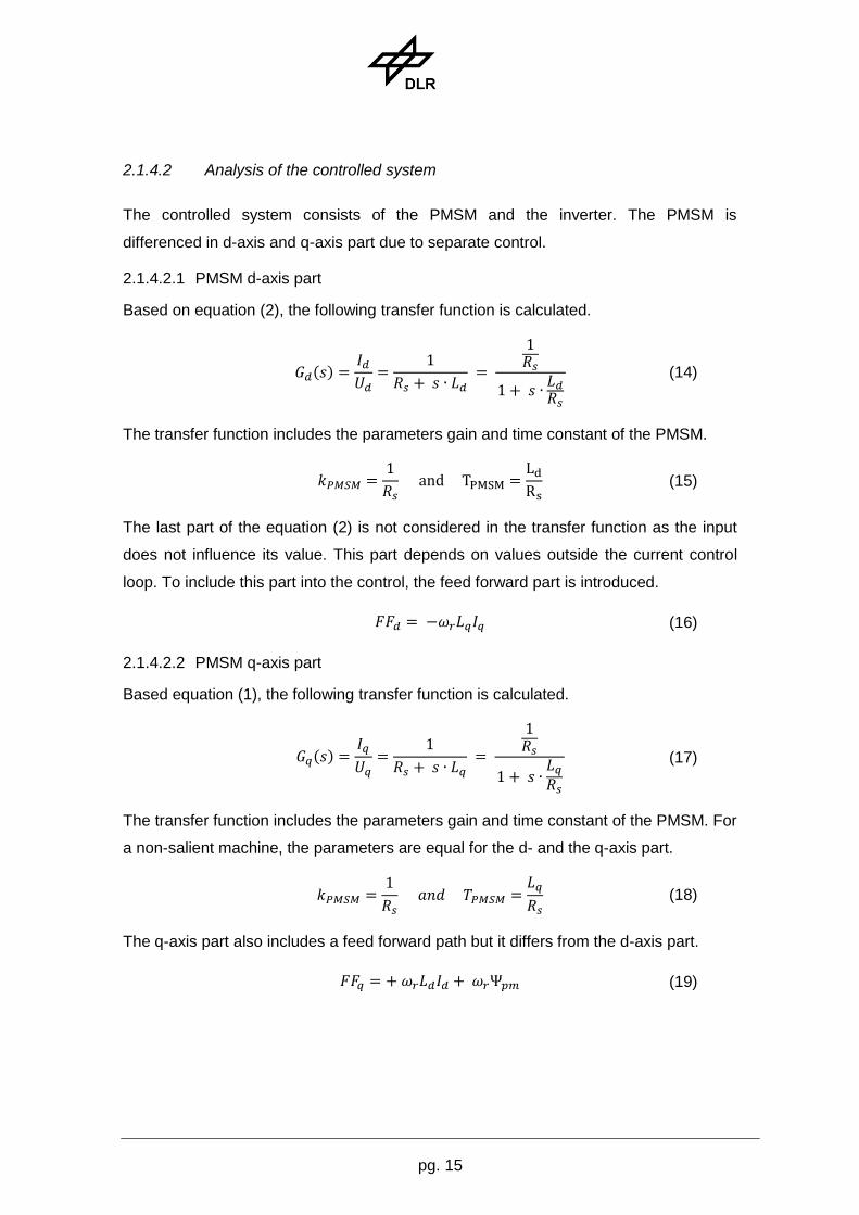
2.1.4.2 Analysis of the controlled system
The controlled system consists of the PMSM and the inverter. The PMSM is
differenced in d-axis and q-axis part due to separate control.
2.1.4.2.1 PMSM d-axis part
Based on equation (2), the following transfer function is calculated.
(14)
The transfer function includes the parameters gain and time constant of the PMSM.
(15)
The last part of the equation (2) is not considered in the transfer function as the input
does not influence its value. This part depends on values outside the current control
loop. To include this part into the control, the feed forward part is introduced.
(16)
2.1.4.2.2 PMSM q-axis part
Based equation (1), the following transfer function is calculated.
(17)
The transfer function includes the parameters gain and time constant of the PMSM. For
a non-salient machine, the parameters are equal for the d- and the q-axis part.
(18)
The q-axis part also includes a feed forward path but it differs from the d-axis part.
(19)

pg. 16
2.1.4.2.3 Inverter
The DC/AC converter is based on pulse-width-modulation (PWM) with a certain
frequency fPWM respective a certain time period TPWM. It can be approximated with PT-1
behaviour. (3)
(20)
2.1.4.3 Equations of the PMSM in Rotor Reference Frame
The characteristics of the stator voltages are described by the following equations (3).
(21)
2.1.4.4 Controller Design
The controller design plays an important role for the controlled system and depends on
the desired behaviour of the systems. There are some requirements which can be
weighted differently:
Steady-state accuracy
Dynamic accuracy
Consequences of disturbances
The design of a controller is always a compromise between stability, accuracy and
dynamic behaviour. A higher gain, for example, results in a better accuracy but also
reduces the stability behaviour.
Two standard control design techniques are the magnitude optimum and the
symmetrical optimum (3). The magnitude optimum claims the following requirement:
The magnitude of the closed-loop frequency response shall be ideal in a preferably
wide range, i.e. the control shall be very accurate until very high frequencies. This
results in very low overshoots and a fast regulation of disturbances. Thus, it is
appropriate for non-oscillating systems. The current of the PMSM with its not negligible
dynamic behaviour of the inverter meets the requirements to be controlled by a
controller designed using the magnitude optimum.
The magnitude optimum determines the parameters of a controller with proportional
and integral gain. The PI controller is described by the transfer function

pg. 17
(22)
The parameters for the PI controller are chosen following the rules in (3)
Compensation of the bigger time constant with the time constant of the PI controller:
The controlled system consists of two PT1 blocks with the time constants TPMSM and
TPWM. Thereby, the time constant TPMSM is bigger than the time period of the inverter.
(23)
Determination of the gain of the PI controller which enables the transfer function to
be one in a very large frequency range.
(24)
The magnitude optimum optimises the current control for high accuracy.
The use of a PI controller for this system has got two advantages. Firstly, the largest
time constant of the controlled system is compensated. That is a requirement to
achieve the best possible dynamic behaviour. Secondly, the integral part of the
controller prevents a remaining error between reference value and actual value.
Including the designed current controller in the system, the transfer function of the open
control loop is
(25)
The feedback of the current closes the loop and leads to the following transfer function
of the whole current control system:
(26)

pg. 18
As
is much smaller than one, the part including s² is negligible. The
result is a substitute current transfer function for further calculations with the
following characteristics
(27)
2.1.5 Current Reference Generation
The stator current reference in d-axis and q-axis is calculated in a Current Reference
Generator block. The input of this block is a torque demand; the outputs are the d-axis
current reference and the q-axis current reference. In this block, current and voltage
limitations are considered.
2.1.5.1 Maximum Torque per Ampere
The most important aim of the Current Reference Generator is the consideration of
voltage and current limitations. If these requirements are met, the requested torque
should be provided with a minimisation of the losses. The minimisation means highest
efficiency and is achieved by using the minimal stator current for the requested torque.
The Maximum Torque per Ampere (MTPA) current reference generation depends on
the saliency of the PMSM.
2.1.5.1.1 Non-salient machines ( )
The inductances in the rotor reference frame depend on the arrangement of the
permanent magnet in the rotor. A non-salient PMSM has the same values for the
inductances in d-axis and in q-axis.. That simplifies the torque equation (3) to
(28)
Then, the provided torque just depends on the current in q-axis. That means the stator
current which is a result of the d-axis and the q-axis current can be minimised by
setting the d-axis current to zero.
(29)

pg. 19
(30)
2.1.5.1.2 Salient machines ( )
Salient machines have an unsymmetrical arrangement of the permanent magnet in the
rotor and its inductances in d-axis and q-axis do not have the same value. That
complicates the MTPA current reference generation. The calculation is explained very
detailed in (3). The minimisation of the stator current considers the following two
equations.
√
(31)
[ ( ) ] (32)
2.1.5.2 Voltage Limitations
With increasing speed, the induced voltage also increases because it is proportional to
the rotational velocity .. The higher induced voltage requires a supply of the PMSM
with a higher voltage. The requested voltage of the Current Control output may become
higher than the voltage that can be provided by the inverter. The output of the inverter
is limited by the DC link voltage.
The induced voltage also depends on the magnetic flux. In general, it is possible to
decrease the magnetic flux in order to enable the machine to run at higher speed. This
procedure is called field weakening. As a PMSM has got permanent magnets in its
rotor, a field weakening in the common way is not possible. Normally, the exciting
current for the magnetic flux is reduced and thus field weakening achieved. In the
PMSM, there is another way to weaken the effect of the permanent magnets. By
introducing a negative d-axis current , a magnetic flux is created that counteracts the
permanent magnets. From outside, this can be regarded as field weakening.
The maximum voltage that can be created by the inverter is limited by the available
voltage from the DC link. As the electrical machine operates in star connection, the DC
link voltage has to be divided by the square root of 3.
√ (33)
The absolute requested voltage must not be higher than the maximum available
voltage.

pg. 20
√
(34)
The voltages and depend on the stator currents and as described in
equations (1) and (2). For high speed, the voltage part that occurs at the resistance
is negligible as it is rather small. This assumption leads to the following equations.
(35)
The equations in (35) can be plugged in equation (34).
√
( )
( )
(36)
2.1.5.2.1 Non-salient machines
For non-salient machines ( ), the following equation is valid.
(
)
(37)
This equation symbolises an equation of a circle in a stator current graph. The two
axes are the currents Id and Iq. The circle of the voltage limit has got the characteristics:
Centre: (
)
Radius:
The centre of the circle depends only on the properties of the electrical machine. A
higher magnetic flux of the permanent magnet results in a higher induced voltage.
Thus the voltage limitations are stricter. In contrast, the radius is dependent on the
current rotational speed of the electrical machine. With increasing speed, the radius of
the voltage limit circle shrinks. The result is a speed dependent voltage limit circle. The
operating point has to be within the circle to meet the voltage limit requirements.
2.1.5.2.2 Salient machines
For salient machines ( ), the equation becomes the following.

pg. 21
(
)
(
) (38)
This is not the equation of a circle anymore, but the equation of an ellipse in a stator
current graph. The ellipse has got the characteristics:
Centre: (
)
D semi axis:
Q semi axis
Here, the centre is independent of the rotational speed as well. The semi axes of the
ellipse depend on the speed and the inductances. It results in a speed dependent
voltage limit ellipse. For higher speed, the ellipse shrinks. To meet the voltage limit
requirements, the stator current has to be within this ellipse. (2)
2.1.5.3 Current Limitations
The most important requirement is the stator current limitation to protect the electrical
machine against damage. The absolute stator current, depending on the d-axis and the
q-axis current, has to be smaller than the maximum allowed current for the machine.
√
(39)
When the current limit is reached, the q-axis current has to be reduced. That results in
a decreased available torque. The equation (39) can also be interpreted in the stator
current graph. It symbolizes a circle with the centre in the origin and the radius Imax.
2.1.5.4 Stator Current Graph
The sections 2.1.5.1 to 2.1.5.3 can be summarised in one stator current graph in the
rotor reference frame (dq). Figure 9 shows an example of the stator current graph for a
non-salient PMSM. The graph consists of the axes for the currents and . As the
machine is non-salient, the provided torque just depends on the supplied q-axis current
. The Maximum Torque per Ampere (MTPA) locus in red is orthogonal to the d-axis
current and the loci for a constant torque (green) are parallel to the d-axis current. The
q-axis current and the provided torque are correlated by the equation (28). The red
circle symbolises the stator current limit which is a machine specific value. The blue

pg. 22
circles indicate the speed dependent voltage limits. As the speed increases, the
voltage limit circles shrink. The operating point has to be within the red circle and the
currently valid blue circle. This graph shows the need of field weakening for high speed
to meet the voltage limitations. (2)
Figure 9 - Stator current graph in dq frame
The requirements for the current reference generation as described above are different
in the priority. Most important is the requirement to stay within the current limitations.
This is necessary to protect the electrical machine and the power electronics. Staying
within the voltage limitations is the second priority. As the DC link supply is limited, the
supply of the electrical machine is limited as well. If these requirements are met, the
purpose is choosing the minimal stator current for a given torque (MTPA). This
corresponds to the highest possible efficiency.
2.1.5.5 Field Weakening Control
The field weakening control is required to satisfy the voltage limitations. Therefore, the
requested voltage which is the output of the Current Control block has to be monitored.

pg. 23
When the absolute requested voltage comes close to the maximum available voltage,
the field weakening is started.
The margin is defined to be 95% of the available voltage from DC link. This gives some
reserve in the case of fast voltage variations. When the margin is reached, a PI
controller starts to decrease the d-axis current reference for the current controller. That
influences the d-axis and the q-axis voltage and thus the absolute requested voltage.
The PI controller output has its upper limit at zero; that means only negative current is
allowed for field weakening. The purpose of the controller is to adapt the d-axis current
so that the voltage limit is not exceeded. The parameters of the controller are chosen in
a way that the controller does not behave too aggressive. As the speed variation is
limited due to inertia of the vehicle, the field weakening does not have to adapt very
fast. The mechanical side with the inertia and the mass of the vehicle reacts much
slower than the electrical side with its inductances. A PI controller with gain 0.1 and the
time constant 0.1s shows a good behaviour in the simulations.
2.1.5.5.1 Normal operation
With increasing speed, the requested absolute voltage increases because of the
speed dependent induced voltage. The d-axis current is equal to zero and the q-axis
current is adapted to provide the requested torque. It is constant for a constant
torque and the determination follows the Maximum Torque per Ampere concept.
2.1.5.5.2 Field weakening operation
At a certain point of speed, the maximum absolute voltage is reached. With further
increasing speed, field weakening is started. The q-axis current Iq remains constant for
providing a constant torque. In contrast, the d-axis current becomes more and more
negative to cause the field weakening effect. As a result, the requested absolute stator
current increases. The d-axis voltage becomes more negative and the q-axis
voltage decreases due to the increasing negative d-axis current , but the absolute
voltage remains constant in field weakening operation. The behaviour of the stator
voltages and the stator currents can be comprehended by regarding the equations (1)
and (2).
Field weakening is not very efficient for PMSM but it is a possibility to drive with slightly
higher speeds for some time. Figure 10 shows graphs of the stator voltages and the
stator currents in the field weakening operation. The electrical machine provides a

pg. 24
constant torque of 40 Nm. Up to the speed of about 1000 rpm, the PMSM is in normal
operation mode. Then, the maximum available stator voltage is reached and field
weakening is started. The graphs show the constant remaining stator voltage , the
constant remaining q-axis stator current and the negative increasing d-axis stator
current for achieving the field weakening effect.
Figure 10 - Stator voltages and currents in dq frame for field weakening control
This graph only shows theoretical possibilities. It is not common to run a PMSM with
speed that is a lot of higher than the nominal speed due to non-efficient characteristics.
The speed range shown in the graphs is thus exaggerated.
2.1.6 Speed Control
The speed control of the electrical drive is realised as cascade control. The speed
control loop is constructed around the current control loop which is described in 2.1.4
and designed in 2.1.4.4. The controlled system of the speed control consists of the
current control loop and the inertia of the electrical machine. It is denoted in (40). The
current control loop is approximated by the substitute current transfer function that is
described in the equation (27). The inertia of the electrical machine acts as integrator
with the time constant described in (41).
(40)
(41)
A controller with proportional and integral gain is used. The transfer function of the PI
controller is the following.
pg. 25
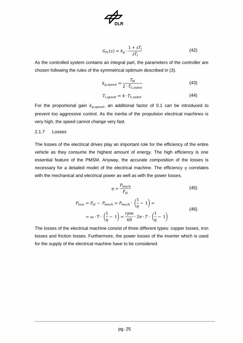
(42)
As the controlled system contains an integral part, the parameters of the controller are
chosen following the rules of the symmetrical optimum described in (3).
(43)
(44)
For the proportional gain , an additional factor of 0.1 can be introduced to
prevent too aggressive control. As the inertia of the propulsion electrical machines is
very high, the speed cannot change very fast.
2.1.7 Losses
The losses of the electrical drives play an important role for the efficiency of the entire
vehicle as they consume the highest amount of energy. The high efficiency is one
essential feature of the PMSM. Anyway, the accurate composition of the losses is
necessary for a detailed model of the electrical machine. The efficiency correlates
with the mechanical and electrical power as well as with the power losses.
(45)
(
)
(
)
(
)
(46)
The losses of the electrical machine consist of three different types: copper losses, iron
losses and friction losses. Furthermore, the power losses of the inverter which is used
for the supply of the electrical machine have to be considered.

pg. 26
Mechanical Losses (Friction)
Mechanical Power
Electrical Power
Inverter Losses
Copper Losses
Iron Losses
Figure 11 - Composition of the losses of a PMSM
2.1.7.1 Copper Losses
The conducting losses in the coils of the electrical machine are called copper losses.
The losses depend on the current and thus on the provided torque. As the rotor
includes permanent magnets, it does not have to be magnetised and there are no
copper losses in the rotor. That explains the high efficiency of the PMSM. The copper
losses are denoted in the following equations. The resistor symbolises the
resistance of one stator winding.
(47)
√
(48)
2.1.7.2 Iron Losses
As the copper losses of a PMSM are reduced in comparison to a synchronous
machine, the iron losses constitute a larger portion of the total losses. The iron losses
basically consist of two different types of losses, the hysteresis losses and the eddy
current losses. The effects are explained detailed in (8)and (9). The excess eddy
current losses are relative small and are negligible for the regarded PMSM. The origin

pg. 27
for all the loss mechanism is the Joule loss due to the eddy currents which results from
changing the magnetisation.
2.1.7.2.1 Hysteresis Losses
Hysteresis losses result from the Backhausen effect. Small domain wall segments
make localized jumps between local minima of the system of free energy, giving rise to
localized eddy currents around the jumping wall segments. The effect is proportional to
the frequency respective to the rotating speed of the machine.
2.1.7.2.2 Eddy Current Losses
These losses are associated with a uniform change of the magnetisation throughout
the sample. The resulting eddy currents flow throughout the body of the sample. The
eddy current losses are proportional to the square of the frequency.
Both the hysteresis and the eddy current losses can be summarised by the following
equation. The parameters and are machine specific. They can be obtained
by measurements which is much easier than the calculation.
(49)
2.1.7.3 Friction Losses
In every rotating or moving system, friction losses occur. In an electrical machine, the
frictional losses are proportional to the rotational speed. The friction losses normally
are very small in compare to the copper and iron losses. The parameter
depends on the construction of the machine.
(50)
2.1.7.4 Inverter Losses
The inverter supplies the PMSM with the requested voltage. Therefore, the DC link
voltage is converted to a three-phase voltage. Figure 12 shows the basic schematics of
a DC/AC converter. There are six IGBT transistors, each with freewheeling diode. They
are arranged in three branches and the middle of each branch is the output for one
phase of the three-phase AC voltage. The appropriate control enables the conversion
from the constant DC voltage to the requested three-phase voltage.

pg. 28
Figure 12 - Power module schematics
Both in the IGBT and in the free-wheeling diode, power losses occur. The main losses
of the IGBT are the switching losses when the transistor is turned on or turned off.
Furthermore, there are conducting losses when current flows through the IGBT. The
forward blocking losses and the driver losses are rather small and negligible. The free-
wheeling diode also creates turn-off losses and conducting losses. The reverse
blocking power losses are negligible.
The inverter losses can be approximated by two parts. One part is constant and
independent of the current flowing through the transistor, on condition that the
switching frequency is constant. That mainly includes the switching losses. The other
part depends on the current flowing through the components. The conducting losses
are influenced by that. (10) (11)
The implementation of the inverter losses in the model are approximated by the
equation (51). The constants and are inverter specific.
(51)
2.1.8 Modelica Model
The Modelica Standard Library, Version 3.1, which is provided by the Modelica
Association contains a model of a PMSM (SM_PermanentMagnet). Resistance and

pg. 29
stray inductance are modelled directly in the stator phases, frame transformations and
a rotor fixed air gap model are used to provide a torque to the flange. The permanent
magnet is modelled by a constant equivalent excitation feeding the d-axis current of the
rotor. Only the losses in stator resistance are considered which are equal to the copper
losses (see 2.1.7.1). (12)
2.1.8.1 Iron Losses
For an accurate model of the PMSM, only the consideration of the copper losses is not
sufficient. Especially, the influence of the iron losses is not negligible as it becomes
even the largest part of the losses at high speed. The composition of the iron losses
are explained in 2.1.7.2. The iron losses consist of one part which is proportional to the
speed and one part which is proportional to the square of the speed. As the mechanical
power is the product of angular velocity and torque, the iron losses can be expressed in
another way. The iron losses can be seen as an additional torque that the electrical
machine has to provide. One part of the torque is constant and the other part is linear
speed dependent.
The bearing friction is an element of the Modelica Standard Library and describes the
coulomb friction in bearings. The friction torque is a function of the angular velocity
which is noted in a table and the element is connected to the flange of the electrical
machine.
The implementation of the iron losses as bearing friction and torque source and is
shown in Figure 13. Both elements are from the Modelica Standard Library. The
bearing friction describes the hysteresis losses. The torque source implements the
eddy current losses as linear speed dependent torque. The torque is the opposite
direction for the opposite direction of the rotation. The flanges of the bearing friction
and the torque source are connected to the output flange of the electrical machine.

pg. 30
Figure 13 - Modelica model of the iron losses
2.1.8.2 Functional Inverter
The inverter converts the DC link voltage to the supply voltage of the PMSM. The input
of the inverter block is the requested voltage that is calculated by the current controller.
The requested voltage is described in the rotor reference frames and consists of the
voltage in d-axis and the voltage in q-axis. The aim of the inverter is to provide the
requested voltage to the PMSM. Thereby, the functional inverter considers the inverter
losses and the discharging of the DC link voltage. The output voltage of the inverter
depends on the model of the PMSM. Functional means that there are no switching
elements included in the inverter. The conversion is a mathematical calculation that
represents the real inverter.
2.1.8.2.1 Inverter for a PMSM in three-phase stator reference frame (abc)
The supply voltage of this model is a three-phase AC voltage. First, the inverter
transforms the requested voltage from the rotor reference frame into the three-phase
stator reference frame 0. The requested voltage is delayed by a PT1 element with a
time constant that is equal to the period of the pulse-width modulation of the inverter.
Afterwards, this three-phase voltage is provided to the output. For the power flow on
the DC link, the following equation is considered.
(52)
2.1.8.2.2 Inverter for PMSM in rotor reference frame (dq)
The PMSM model in rotor reference frame is supplied by a d-axis voltage and a q-axis
voltage. The requested voltage is also delayed by a PT1 element with a time constant
that is equal to the period of the pulse-width modulation of the inverter. For the

pg. 31
calculation of the power on the DC link side, the definition of the rotor reference frame
in chapter 2.1.2.3 leads to the introduction of a factor 3/2. The power relations are
shown in the following equation.
(53)
2.1.8.3 PMSM Model in rotor reference frame
The PMSM model in rotor reference frame extends from the partial basic machine
which is modelled in the Modelica Standard Library. The base partial model for DC
machines contains the inertias, the mechanical shaft and the mechanical support. The
other elements of the PMSM have to be added. The air gap model converts the
supplied voltage into torque at the flange. The conversion takes place according to the
equations (1) to (3). As described in 2.1.8.1, the iron losses are introduced as a torque
load at the flange of the rotor. The connection to the inverter is realised by a “dq plug”.
This plug contains two voltages and currents, one for the d-axis and one for the q-axis.
The rotor inductances consist of a main field inductance and a stator stray inductance
.
(54)
The stator stray inductance does not influence the torque generation but has an
influence on the voltage. The voltage across the stator stray inductance is denoted by
the following equations.
(55)
The effects of the stator stray inductance are modelled in the element Lssigma dq.
Figure 14 shows the entire model of the PMSM in rotor reference frame.

pg. 32
Figure 14 - PMSM Modelica model in rotor reference frame (dq)
2.1.8.4 Simulation Results
2.1.8.4.1 Absolute Power Losses
Figure 15 shows the absolute power losses of the Modelica model and the motor data
from the manufacturer. The losses increase with higher speed due to the iron losses. A
higher torque requires a higher current which results in higher copper losses. This
example shows one propulsion motor of the electric vehicle. The simulation results
(blue graph) are very similar to the data from the manufacturer (red graph). Only for
very low speeds, there are some power losses effects that are not considered in the
model. As this region corresponds to very low speed and is not the main operating
point, these deviations are neglected. The standard Modelica models of electrical
machines only consider the copper losses (black graph). This assumption results in
absolute power losses independent of the rotational speed. That leads to a very high
efficiency for high speeds which is not realistic and far from the data of the
manufacturer.

pg. 33
Figure 15 - Absolute power losses
2.1.8.4.2 PMSM model in rotor reference frame
Figure 16 shows the DC link current and the difference between the usage of the
PMSM model in the stator reference frame (abc) and the PMSM model in the rotor
reference frame (dq). Both models, the PMSM model in the stator reference frame from
the Modelica Standard Library and the PMSM model in the rotor reference frame,
behave exactly the same way. For the same reference, they generate the same speed
and the same torque at the flange. The power consumption is identical, too.
The only difference occurs in the current consumption on the DC link voltage. As the
PMSM model in stator reference frame is supplied by a three-phase alternating current
(AC), the current consumption oscillates on the DC link, too. The root mean square
(RMS) value of the power consumption is identical for both machines. Consuming DC
current instead of AC current is easier to handle and faster to simulate. The simulator
does not have to use an integrator step size to follow 20 to 1000 Hz signals but just
uses the RMS value. Thus a much bigger integrator step size is possible and the
simulation is more efficient.

pg. 34
Figure 16 - DC link current PMSM dq and abc
For this example of the simulation of a PMSM, the simulation time is reduced by a
factor of 2.5. In the simulation of the entire vehicle model, it would result in a higher
factor as the small step size of the PMSM abc must be applied for the entire model.
0 5 10 15 200
5
10
15
20
25
30DC link current PMSM dq und abc
Time [s]
Cu
rre
nt
[A]
PMSM abc
PMSM dq

pg. 35
2.2 Sensor data fusion for the use in Real-Time systems
For model based control, like the here proposed Energy Management, the system
states of the vehicle must be reliably available. Unfortunately, many of them cannot be
measured directly and therefore have to be estimated. In the following sections,
different recursive state estimation algorithms are investigated and the interconnection
between them derived. The most common algorithms are sketched as pseudo code
algorithms and the difference between them are explained. In the second part an
application using the example of a battery state of charge estimation is given. These
algorithms are part of a battery management system, which are implemented on
embedded controllers in today’s electric vehicle. The aim of these systems is to give a
good estimation for actual and future power availability and health monitoring. This
requirement is very complex due to the nonlinear behavior, especially in the case of
high performance Lithium-Ion cells. Currently no direct measurement method without
destroying the cell to determine the system’s states, like the SOC, is available.
Therefore here a real-time capable model that is combined with recursive online
estimation is suggested, which gives a good trade-off between modeling accuracy and
real-time requirements. The proposed algorithm is successfully implemented,
parameterized and tested on the DLR RMC ROboMObil research platform (Figure 17,
(13)). Finally, simulation results with real world drive cycles to validate the performance
and quality are given.
Figure 17: ROMO – the robotic electric vehicle in front of DLR Techlab

pg. 36
2.2.1 Recursive state estimation
In this chapter, the principle ideas of recursive state estimation are summarized, and its
(historical) development leading to the Kalman Filter is outlined. In the second part, this
algorithm is extended to nonlinear systems and finally the latest developments are
sketched. Further background information, alternative formulations, and recent
developments are provided in the standard book (14) that is also the starting point for
the following explanations.
2.2.1.1 Principles
At first, we consider an estimation of a constant signal on the basis of several noisy
measurements. This Weighted Least Squares Estimation problem is well-known in
system identification tasks (see, e.g., (15)). Through the weighted formulation, the user
can assign different levels of confidence to certain measurements (or observations).
This feature is crucial for tuning Kalman Filters. The corresponding minimization
problem is formulated as follows:
[
] [
] [
] [
]
( )
(56)
The unknown vector is constant and consists of elements, is a -element noisy
measurement vector and usually . Each element of y - - is a linear combination
( ) with the unknown vector x and the variance of the measurement noise of the i-th
measurement . The noise of each measurement is zero-mean and independent from
each other, therefore the measurement covariance matrix is
(57)
The residual
⏟
(58)
is the difference of all measured values y with the (unknown) x-vector minus the
estimated vector that is computed from the estimated vector . The goal is to

pg. 37
compute the estimated vector such that the weighted residual is as small as possible,
i.e., to minimize the cost function J:
(59)
To minimize , it is useful to compute the partial derivative with respect to the estimated
vector and set it to zero. In this way, an optimal solution for can be calculated:
(60)
(60) requires that R is nonsingular and H has full rank. This is the “textbook” version of
the algorithm. It is inefficient and numerically not reliable. Alternatively, (59) can be
formulated as:
[
]
[
]
(61)
To solve the following standard linear least squares problem that minimizes the
Euclidian norm of the weighted residue vector:
‖ [
] ‖
‖ ‖
‖ ‖
‖ ‖
(62)
This minimization problem has a unique solution, if A=WH has full rank. If A is rank
deficient, an infinite number of solutions exists. The usual approach is to select from
the infinite number of solutions the unique one that additionally minimizes the norm of
the solution vector: ‖ ‖ Given A= WH and b = Wy, this solution vector can be
computed with the Modelica function Modelica.Math.Matrices.leastSquares(...) from the
Modelica Standard Library which is a direct interface to the LAPACK function DGELSX
[Lap99]. This function uses a QR decomposition of A with column pivoting together with
a right multiplication of an orthogonal matrix Z to arrive at:

pg. 38
‖[ ] [
] ‖ (63)
where Q and Z are orthogonal matrices, P is a permutation matrix, U is a regular, upper
triangular matrix and the dimension of the quadratic matrix U is identical to the rank of
A. Since the norm of a vector is invariant against orthogonal transformations, this
equation can be transformed to:
‖ [
] [
] ‖ (64)
This is equivalent to
‖[ ] [
] ‖ = (65)
from which the solution can be directly computed as (taking into account b = Wy):
(66)
In the following, only textbook versions of algorithms will be shown, such as (60). Their
implementation is, however, performed in an efficient and numerically reliable way,
such as (66), where matrices R and H can be rank deficient. The sketched approach,
both (60) and (66), can be used for offline estimation with a predetermined number of
measurements k. In real-time applications, new measurements arrive in each sample
period to improve the estimation. Using (66) would require a complete recalculation
with -flops. One approach could be to use a moving horizon and to forget the
older measurements (still costly). Another option is to reformulate the problem into a
recursive form that is updated at every sample instant with the new measurements. A
linear recursive estimator can be written in the following representation:
(67)
We compute based on the estimation from the last time step and the
information from the new measurement . is the estimator gain vector that weights
the correction term . Hence, we have to compute an optimal in a
recursive way. To this end, it is necessary to formulate another cost function that
minimizes the covariance in a recursive way.
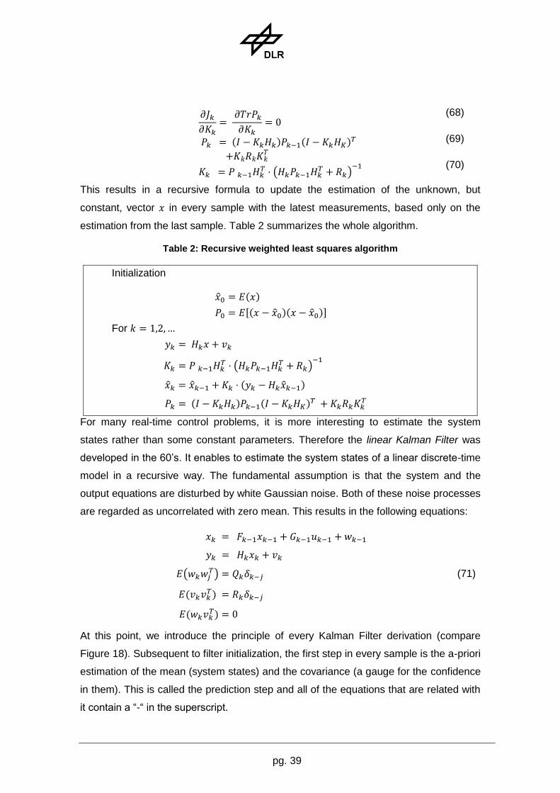
pg. 39
(
)
(68)
(69)
(70)
This results in a recursive formula to update the estimation of the unknown, but
constant, vector in every sample with the latest measurements, based only on the
estimation from the last sample. Table 2 summarizes the whole algorithm.
Table 2: Recursive weighted least squares algorithm
Initialization
[ ]
For
(
)
For many real-time control problems, it is more interesting to estimate the system
states rather than some constant parameters. Therefore the linear Kalman Filter was
developed in the 60’s. It enables to estimate the system states of a linear discrete-time
model in a recursive way. The fundamental assumption is that the system and the
output equations are disturbed by white Gaussian noise. Both of these noise processes
are regarded as uncorrelated with zero mean. This results in the following equations:
( )
(71)
At this point, we introduce the principle of every Kalman Filter derivation (compare
Figure 18). Subsequent to filter initialization, the first step in every sample is the a-priori
estimation of the mean (system states) and the covariance (a gauge for the confidence
in them). This is called the prediction step and all of the equations that are related with
it contain a “-“ in the superscript.

pg. 40
Time Update
(Predict)
Measurement
Update
(Correct)
kx
kxy
00 ,ˆ Px
Figure 18: Principle of recursive Kalman filter.
This forms the basis for the calculation of the optimal Kalman gain that is used to
correct the estimated state vector with the information from the actual measurements.
Finally, the covariance matrix is updated. This is called the correction step. In the next
sample, these values are used to restart again at the subsequent prediction step. The
algorithm can be formulated as follows:
Table 3: Linear discrete Kalman Filter
Initialization
[
]
For
(
)
To determine the relationship between the Kalman Filter and recursive weighted lest
squares, we should have a closer look at Table 3. The matrix
represents the covariance of the system states (
denotes the variance of the system states). Its entries represent the confidence in the
a-priori estimation and can be tuned by the application engineer. Large values
represent high uncertainty (probably due to an imprecise model), whereas small values
indicate good trust. The second tuning matrix represents the confidence in the actual
measurements. Its effect resembles our first estimation problem (eq. (56) to (60)).

pg. 41
Furthermore, it can be shown that if is a constant vector then and
. In this case, the Linear discrete Kalman Filter algorithm (Table 3) reduces to
the recursive weighted least squares algorithm (Table 2). This property is often
exploited in the formulation of parameter estimation problems using Kalman Filter
algorithms.
2.2.2 Nonlinear Kalman Filter Algorithms
So far, we have discussed estimation problems for linear discrete systems. This is
generalized to nonlinear systems starting from a continuous-time representation in
state space form:
(72)
In section 3, it is sketched how such a model description can be generated from a
Modelica model for use in a nonlinear Kalman Filter using the Functional Mockup
Interface. In this way, it is possible to formulate the synthesis models for the prediction
step (see Figure 18) with Modelica, even in implicit representation, and shift all tedious
tasks to the Nonlinear Observer framework. This avoids calculus mistakes and allows
us to put the main focus on the design of the algorithms.
In Table 4, the widely used extension of the discrete linear Kalman Filter to the discrete
nonlinear Kalman Filter with additive noise is presented. The dynamic system is
represented as follows:
(73)
The algorithm is very similar to a purely linear one. To handle the nonlinearity, the
system is linearized around the last estimation point using a Taylor Series Expansion
up to the first term. This can be performed numerically by the use of a forward
difference formula.
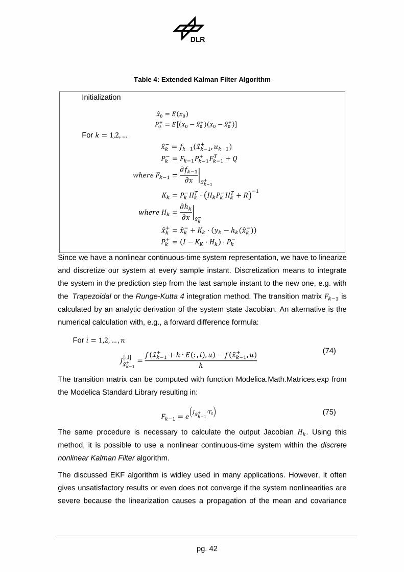
pg. 42
Table 4: Extended Kalman Filter Algorithm
Initialization
[
]
For
|
(
)
|
Since we have a nonlinear continuous-time system representation, we have to linearize
and discretize our system at every sample instant. Discretization means to integrate
the system in the prediction step from the last sample instant to the new one, e.g. with
the Trapezoidal or the Runge-Kutta 4 integration method. The transition matrix is
calculated by an analytic derivation of the system state Jacobian. An alternative is the
numerical calculation with, e.g., a forward difference formula:
For
[ ]
(74)
The transition matrix can be computed with function Modelica.Math.Matrices.exp from
the Modelica Standard Library resulting in:
(
)
(75)
The same procedure is necessary to calculate the output Jacobian . Using this
method, it is possible to use a nonlinear continuous-time system within the discrete
nonlinear Kalman Filter algorithm.
The discussed EKF algorithm is widley used in many applications. However, it often
gives unsatisfactory results or even does not converge if the system nonlinearities are
severe because the linearization causes a propagation of the mean and covariance

pg. 43
that is only valid up to the first order. The following section sketches the principles of
the Unscented Kalman Filter (UKF) and its advantages in nonlinear state estimation.
2.2.2.1 Unscented Kalman Filter
In order to achieve higher accuracy, the UKF calculates the means and covariances
from disturbed state vectors, called sigma points, by using the nonlinear system
description. As one side effect, the Jacobians of and are no longer needed.
See (16)for more detailed information. The structure of the equation set, containing
prediction and update, is similar to the EKF. However, the calculation of the
covariances requires to integrate the nonlinear system times from the last to the
actual time instant and is therefore computationally costly. The symmetry of all the
involved matrices is fully exploited to reduce computational costs. An additional
reduction of computational effort is achieved with the Square Root UKF (SR-UKF).
2.2.2.2 Square Root Unscented Kalman
The equations of the SR-UKF are identical to the UKF, but the structure is utilized
during the evaluation: Although the covariance matrix and the predicted covariance
matrix are uniquely defined by their Ckolesky factors √ and √
respectively, with
UKF the covariance matrices are calculated at each step. Furthermore, the sigma
points can be computed with the Cholesky factor √ , and the updated sigma points
of the measurement update with the Cholesky factor √ without using the covariance
matrices. Moreover, the gain matrix is determined as solution of the linear equation
system
(76)
that can be more efficiently solved by utilizing again the Cholesky factorization. In the
SR-UKF implementation, the Cholesky factors are propagated directly and the
refactorization of the covariance matrices is avoided (17).
The EKF, UKF, and SR-UKF algorithms are implemented as Modelica functions using
LAPACK for core numerical computations. Implementation details of the numerical
algorithms will be provided in an upcoming publication by Marcus Baur.

pg. 44
2.2.3 Battery models for online purposes
Now we come from the theory of the different Kalman Filters to the second part of this
chapter. Here we derive an improved and optimized battery model for an estimation
task in a battery electric vehicle.
Nowadays Batterie Management Systems for BEV, e. g. the widely used system from
I+ME Actia, use a predetermined cell characteristic table and a current counting
method without considering the transient behavior of the cell.
Another and more advanced approach is the Enhanced Self Correcting Model
proposed by Plett in (18), (19), (20)and (21). The cell is considered as a system with
input "cell current" and output "terminal voltage". The State Of Charge is included in
the state vector and therefore can be estimated by means of an EKF. The basis of the
model is the open-circuit voltage and the ohmic loss. This is represented in the
equivalent circuit in Figure 19.
UOCV ucell
icellRi
Figure 19: Equivalent circuit representation
Beyond that, this approach takes into account hysteresis effects. The remaining cell
dynamics is described by means of a current filter. Therefore, this results in the
following output equation:
(77)
where is the hysteresis voltage and represents the influence of the current filter.
The implementation of the ESC model shows significant optimization potential. There
are several better discretization methods than the proposed explicit Euler 1 method.
This helps in simulation stability and accuracy for online and offline purpose (see
section 2.2.5 for details). The formulation of the current filter also seems unnecessary
complex, It is formulated as an IIR Low Pass Filter as follows:
,.

pg. 45
Furthermore the computational costly online parameterization of the filter by the use of
a dual estimation approach (see (21)) can be done offline. In this way the system order
can be reduced and therefore the online performance increases. Moreover, the first
implementations of the ESC model at DLR have shown problems with the
determination of SOC. In addition, the effects of current and temperature on the actual
cell capacity are not considered in the ESC model. These can have an enormous
influence on the calculation of the SOC, cf. Figure 20.
Figure 20: Capacity variation due to temperature and current ( )
2.2.4 Derivation of an modifiedESC battery model
Since we are convinced of the basic approach with the ESC model, we will introduce a
modified version that is different in several aspects. In the mESC approach, the battery
cell is represented by a continuous state space model. Through this scheme, the
discretization algorithm can be changed and methods with higher accuracy, such as
Runge-Kutta 4, can be used. Due to the complex structure and time consuming
parameterization of the current filter, it is replaced by a critical damping FIR filter that
only contains one parameter. Additionally, the calculation of the SOC is improved by an
empirically determined correction factor that accounts for the dependency of
temperature and current on the actual cell capacity. Lastly, the model is parameterized
using an offline optimization with real training data and then verified by validation data.
2.2.4.1 Formulation and model structure
The mathematical description of the mESC model is given by the following:

pg. 46
[
]
[
|
|
]
(78)
(79)
The differential equation for the SOC depends on the cell current , the nominal
cell capacity , the Coulombic efficiency and the correction factor . This factor
takes into consideration the variation of the cell capacity as shown in Figure 20.
Following (22)the correction factor is determined by:
{
(80)
is a positive constant leading into a straight line for positive cell current, which
intersects the ordinate at . For negative cell current the correction factor is described
by an exponential function. The parameters and are gathered from capacity tests
replacing the simple straight line with more accurate look-up tables. The hysteresis
voltage is described by a more complex equation taking into account the additional
factors (polarization voltage) and (time constant). The remaining four differential
equations describe the optimized fourth order critical damping current filter with the
only remaining parameter and its four states . The output equation (79) is similar
to the ESC model’s output equation but aggregates the influence of the cell current
(ohmic loss and current filter) into one summand.
2.2.4.2 Model parameters and variables
The internal resistance is one of the cell’s descriptive variables, which depends on
SOC, cell current and temperature resulting in a three dimensional look-up table. This
relationship is visualized for room temperature in Figure 21. Considering equation (79)
one can imagine easily that the resulting cell voltage varies highly in case of low SOC

pg. 47
and high currents due to increase of the internal resistance of the cell. In such cases
the cell is in a critical situation and can be damaged irreversible.
Figure 21: Internal cell resistance for T =25°C
Another important cell variable is the OCV, whose characteristic curve incorporates the
relationship between SOC and OCV, as shown in Figure 22. This depiction also shows
the hysteresis effects very well. The blue and red curves are measured during charging
and discharging of the cell with very low currents respectively. This minimizes
excitation of the cell dynamics so that the cell terminal voltage can be considered
unloaded. In addition, the influence of the internal resistance is eliminated during the
data analysis. The polarization voltage is defined as half of the difference between
the two curves and therefore also depends on the OCV.
Figure 22: OpenCircuitVoltage
In Figure 23 the polarization voltage is plotted depending on the temperature. It is
apparent that temperatures below have the highest influence.
Inn
er
resis
tan
ce
Ri
Cell current
icell [A]
StateOfCharge [-]
0 0.1 0.2 0.3 0.4 0.5 0.6 0.7 0.8 0.9 13
3.2
3.4
3.6
3.8
4
4.2
4.4
Charge
Discharge
OCV
StateOfCharge [-]
Ce
ll vo
lta
ge
[V
]
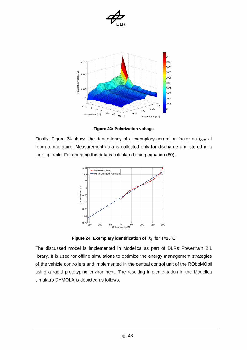
pg. 48
Figure 23: Polarization voltage
Finally, Figure 24 shows the dependency of a exemplary correction factor on at
room temperature. Measurement data is collected only for discharge and stored in a
look-up table. For charging the data is calculated using equation (80).
Figure 24: Exemplary identification of for T=25°C
The discussed model is implemented in Modelica as part of DLRs Powertrain 2.1
library. It is used for offline simulations to optimize the energy management strategies
of the vehicle controllers and implemented in the central control unit of the ROboMObil
using a rapid prototyping environment. The resulting implementation in the Modelica
simulatro DYMOLA is depicted as follows.
StateOfCharge [-]Temparature [°C]
Po
larisa
tio
n v
olta
ge
[V
]
-150 -100 -50 0 50 100 150 2000.75
0.8
0.85
0.9
0.95
1
1.05
1.1
1.15
Measured data
Parameterized equation
Co
rre
ctio
n fa
cto
r k i
Cell current icell [A]

pg. 49
Figure 25: mESC model implementation in DYMOLA
2.2.5 The mESC model and Kalman filtering
The proposed mESC model has one input, cell current, and one output, cell voltage.
These two quantities can be directly measured with high accuracy even in embedded
systems. The third quantity is the cell temperature. It is determined by the use of a
thermocouple sensor on the cell surface. This is the same method as applied in the cell
test bench (see section 2.2.6 for details). To achieve a better estimation performance ,
a second “perfect” measurement equation is implemented. The idea in principal is to
take constraints into account within the Kalman Filter. For this purpose an additional
fictitious measurement is introduced. It can be weighted through the tuning of the
output covariance matrix. This method is well known as Perfect Measurements (ref. to
(14), chp. 7.5.2). In this way the output equation extends to:
[
] (81)
The first equation is identical to formula (79) and the second one can be derived as
follows:
(82)
The measured SOC is calculated through the inverse OCV/ look-up in
combination with a low pass filtering afterwards. This extension allows the KF to adjust
SOC directly and therefore to enforce a physically correct estimation. To use the

pg. 50
proposed mESC model in an embedded system for state estimation a SR-UKF
(chapter 2.2.2.2) algorithm is implemented. It handles the nonlinearities through
statistical linear regression and therefore no numeric derivation of the state and ouput
Jacobians are necessary. In this case, due to the mixed usage of equations and tables,
this optimizes highly the accuracy through the minimization of linearization errors
compared to EKF (chapter 2.2.2). In additional the formulation with matrix updating
techniques ensures a high robustness against non-positive covariance matrix updates.
2.2.6 Parameterization and validation
In the ROboMObil project we were able to obtain a high performance cell from Li-Tec
industries. It has a nominal capacity of 40 Ah and with its security features it is fully
capable for series production. All cell measurement for parameterization, testing, and
validations were done with a Vötsch VT4011 environment simulator and a BaSyTec
battery testing system. The model parameter optimization is accomplished with MOPS
(see (23)for more information) on the Linux cluster of DLR RM Institute. The detailed
procedure and the necessary test cycles are explained in (24). The list of tuned
parameters is given in Table 5.
Table 5: List of optimized parameters
Time constant for rate of change of the hysteresis voltage
Cut-off frequency of the fourth order current filter with critical damping
Cut-off frequency of the first order low pass filter for smoothing the
"measured" SOC needed due to the extended output equation
Covariance matrices for optimal EKF settings (weighting of prediction
by means of the model and correction due to the measured values)
The optimization process can be summarized as shown in Figure 26. As quality
criterions cell voltage and SOC are compared to their respective references using the
so-called fit value. The fit value weights the reference to the simulated characteristic
vector and can be calculated as follows:

pg. 51
(
√∑ (| |
)
√∑ (| ∑
|
)
)
(83)
Since a direct comparison of SOC is not possible, the actually and effectively moved
amount of charge at the terminals of the cell is used.
T Model
Simulation & Analysis
Calculation of quality criterions
Scaling & Weightening
of quality criterions
On-line
visualisation
Optimizer
S
G C
C T: Tuning parameter S: Simulation result G: Quality criterion C: Normed quality criterions
MOPS
On-
linevisualisation
Figure 26: MOPS optimization process
For the validation of the estimated model parameters a test bench experiment by
means of a simulated drive cycle is used. The observer scheme is shown in Figure 27.
The aim is to produce an accurate estimate of the battery SOC, which is a decisive
input for the function of the energy management strategy. In this observer, the input u
of the battery model is the measured current, while the model output ym is the voltage
of a single cell.
V
Observer
I
mESC
+
xKFy
u l
Figure 27: mESC observer structure
The model used in the observer was parameterized by an offline optimization that uses
measurements test cycles and the characteristics of a single cell as training data. In
order to validate the resulting parameterization, the battery was connected to an
electrical power supply/load and tested with a simulated drive cycle. For this simulation,

pg. 52
a model of the longitudinal dynamics of the ROboMObil was developed in Modelica
which calculates the energy flow of all the power consumers in the electrical system
(25).
Figure 28: Artemis Road velocity profile and power consumption
A closed-loop controller calculates the actuator demands in order to follow the specified
driving cycle. In this way, the required electrical power is calculated. Figure 28 shows a
normalized Artemis Road cycle, which is synthesized by stochastic calculations from
real recorded driving data (26). This reflects real driving behavior significantly better
than the purely synthetic ECE15 driving cycle used in the homologation of European
vehicles. The calculated electrical power flow is then taken from a Dymola simulation
and scaled to one battery cell. This data is used on the HIL test bench to give the
Lithium-Ion cell the appropriate load current. The results of this test, including the
current, voltage, as well as the cell temperature are used to test the mESC model with
EKF in the offline simulation. The test results are shown in Figure 29, where the
measured and estimated values are compared to each other. Evidently, the voltage
values agree very well. With almost 93% accuracy, the accordance of the effective
charge amount delivers a good result and shows that the selected approach with the
model-based observer is of practical use.
0 5 10 150
20
40
60
80
100
120
Time [min]
Velo
city [km
/h]
0 5 10 15
-30
-20
-10
0
10
20
30
Time [min]P
ow
er
[KW
]

pg. 53
Figure 29: Experiment results from Artemis Road Drive Cycle Test
2.3 Optimization based operation strategies
In this chapter we focus on the energy optimal control of vehicles powertrain actuators
to follow a given trajectory from a high level planner or an interpreted driver input. This
generic approach utilizes the over-actuated control plant completely to achieve minimal
control effort and therefore best energy efficiency via real-time capable optimization. As
testing platform we choose the DLR RMC robotic electric vehicle (see Figure 17) that is
through its ten powertrain actuators highly predestined for this investigation. The
following chapters are organized as follows: In chapter 2.3.1 the principle idea of the
transfer from robotics to vehicles is sketched. In section 2.3.2 the modeling of the
controlled plant and the derivation of the control allocation (CA) algorithm are stated.
The different implementation and simulation results are given in chapter 2.3.3. Finally
the approaches and further development steps are sketched in section 3.1
2.3.1 ROMO Control – Starting Point, Performance & Enhancements
In (27) we presented a control strategy from the point of view of an easy to handle
Human Machine Interface. The concept is to provide a user-friendly interface to
address the third degree of freedom (DOF) and to distribute the user input to the
overall ten actuators of the ROboMObil. This geometric approach does not take any
further considerations of the actuator dynamics, the losses in the power train or the
wheel slip into account. Although we have experienced good results with the geometric
approach, we decided to develop a new control approach with focus on minimal power
consumption.
0 2000 4000 6000 8000 10000 120003
3.5
4
Reference characteristic
Estimated characteristic (Fit=100.00%)
0 2000 4000 6000 8000 10000 12000
-40
-20
0
Reference characteristic
Estimated characteristic (Fit=92.96%)
Ce
ll vo
lta
ge
[V
]E
ffe
ctive
ch
arg
e
am
ou
nt
Qef
f [A
h]
Time [s]
Time [s]
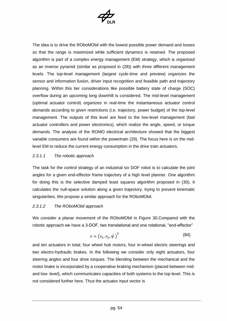
pg. 54
The idea is to drive the ROboMObil with the lowest possible power demand and losses
so that the range is maximized while sufficient dynamics is retained. The proposed
algorithm is part of a complex energy management (EM) strategy, which is organized
as an inverse pyramid (similar as proposed in (28)) with three different management
levels. The top-level management (largest cycle-time and preview) organizes the
sensor and information fusion, driver input recognition and feasible path and trajectory
planning. Within this tier considerations like possible battery state of charge (SOC)
overflow during an upcoming long downhill is considered. The mid-level management
(optimal actuator control) organizes in real-time the instantaneous actuator control
demands according to given restrictions (i.e. trajectory, power budget) of the top-level
management. The outputs of this level are feed to the low-level management (fast
actuator controllers and power electronics), which realize the angle, speed, or torque
demands. The analysis of the ROMO electrical architecture showed that the biggest
variable consumers are found within the powertrain (29). The focus here is on the mid-
level EM to reduce the current energy consumption in the drive train actuators.
2.3.1.1 The robotic approach
The task for the control strategy of an industrial six DOF robot is to calculate the joint
angles for a given end-effector frame trajectory of a high level planner. One algorithm
for doing this is the selective damped least squares algorithm proposed in (30). It
calculates the null-space solution along a given trajectory, trying to prevent kinematic
singularities. We propose a similar approach for the ROboMObil.
2.3.1.2 The ROboMObil approach
We consider a planar movement of the ROboMObil in Figure 30.Compared with the
robotic approach we have a 3-DOF, two translational and one rotational, “end-effector”
( )
(84)
and ten actuators in total; four wheel hub motors, four in-wheel electric steerings and
two electro-hydraulic brakes. In the following we consider only eight actuators, four
steering angles and four drive torques. The blending between the mechanical and the
motor brake is incorporated by a cooperative braking mechanism (placed between mid-
and low- level), which communicates capacities of both systems to the top-level. This is
not considered further here. Thus the actuator input vector is

pg. 55
(85)
In contrast to the robotic approach, we have an under determined optimization
problem. Hence it is possible to exploit the null-space to find an optimal solution, which
minimizes a cost function. This technique is well known as control allocation and it is
used for example in flight applications where the amount of actuators is also larger than
the degrees of freedoms of the body movement (31).
Figure 30: Planar movement of ROboMObil
2.3.1.3 CA enhancements
Due to the fact that CA does not take explicitly system dynamics from the plant or the
actuators into account, those have to be treated separately. In our case we have very
different time constants especially comparing the slower ones belonging to the steering
actuators to the electric ones of the in-wheel motors. Therefore an approach for
compensating the steering actuator time constant is proposed.
2.3.1.4 State of the art
In (32) also the technique of (31) is used in a vehicle CA with EM application. It
proposes a state machine based energy management strategy that distributes the
instantaneous power demand according to rules to the different power sinks and
sources. Force allocation approaches (i.e. (33) (34)) focus on the tire force utilization
factor and optimization of the vehicle dynamics potential and do not have EM as a
primary goal.
2.3.2 The Concept of Energy Optimal Control Allocation
X0
Y0
lr lf
ax
ψ ..
ay
δ2
τ2
F2
δ4
τ4
F4
δ3
τ3
F3
bl
τ1
F1
δ1
br

pg. 56
The technique of CA can be used in a wide range of over-actuated control problems.
The main advantage in comparison to conventional feedback control without
optimization is that it is possible to take actuator limits into account. Due to the control
variable independent design, it is possible to adapt the controller online without
reconfiguring it. For example, in case of an actuator fault the distribution mechanism
can be easily modified to no longer comprise the defective actuating variable.
Furthermore, one can design secondary objectives within the problem formulation. This
opens the possibility to exploit the actuator redundancy for energy optimal actuating
variable determination.
2.3.2.1 CA problem formulation
In Figure 31 a closed loop control allocator scheme is shown. An outer loop controller
determines the virtual control variables based on the desired command variable
reference . These are fed forward to the CA were they are mapped to actuating
variables and then commanded to the over-actuated plant.
Figure 31: Control scheme of closed loop control allocator
The mapping between the virtual control variables and the actuating variables is
concatenated with the so called control actuating variables efficiency function .
Mathematically the general problem formulation of the control allocator can be
considered as follows:
[ ] [ ]
(86)
Here [ ] denote the min/max (rate) actuator limits. There are several methods, to
solve the CA problem for linear systems. The most common ones are daisy chain or
via a cascaded generalized inverse solution (35) (36). As sketched in the beginning of
this section, the goal is to select a method to minimize the costs for two objectives. For
controllercontrol
allocator
over-actuated
plant
vd uydes yact
uact

pg. 57
this reason an optimization based CA is chosen (31). The principle is to minimize a
cost function while handling the CA problem and the limits within the constraints.
Formulated for the linear case, this yields to (35):
(87)
If several solutions for the equality constraints exist, the one that minimizes
the cost function is chosen. In the case there is no solution of the equation
system, the optimization would fail and therefore a second step becomes necessary.
Two of the most common solutions are to “preserve direction”, not discussed here, or
to “minimize the objective error” (35):
(88)
Here signifies the weighting of virtual control variable. Instead of this sequential
optimization approach it can be reduced to a weighted one-step optimization problem
(31).
(89)
The tuning parameter allows the prioritization between the primary and the
secondary optimization objective. By means of the analysis of the controlled
plant (compare section 2.3.1.2) there are strong nonlinearities between the actuating
variables and the virtual control variables. Therefore the proposed method (eq. (87)
and (88)) has to be extended to handle a nonlinear control efficiency matrix (31). For
this purpose the nonlinear CA problem is locally approximated by means of a Taylor
series expansion of the control efficiency function to the first term.
⏟
⏟
(90)
In this way a linear substituted problem for the nonlinear control efficiency function can
be formulated as follows:

pg. 58
(91)
The solution of eq. (91) gives the actuating variables a change to follow the
commanded control variable variation . is the solution approximating
eq. (86). In addition to the linearization of the actuating efficiency function also the
boundaries are substituted to correspond to the actuating variable variation . Since
the CA is used within a time discrete system, the rate of change ⁄ can be
expressed as ⁄ , where constitutes the sample time. To minimize the energy
costs for a virtual control variable trajectory the complete two step optimization problem
is given by:
(92)
In terms of computational effort the solution of the one-step optimization problem (eq.
(89)) may be more efficient, but more difficult to tune. So it is decided to apply the two
step approach (eq.(92)) for controlling the ROboMObil.
2.3.2.2 The actuating variables efficiency matrix
As mentioned before, the actuating variable efficiency function is highly nonlinear. So in
this section the derivation of the linearized matrix is outlined. For the mathematical
description of the vehicle’s planar movement (Figure ) we have two linear momentum
equations and one angular momentum equation. The first two specify the longitudinal
(eq.(93)) and lateral (eq.(94)) movement, the third the rotation around the vertical axis
in the co-ordinate system ( in Figure ).
∑
(93)
∑
(94)

pg. 59
[
]
(95)
Here indicates the vehicle mass, the yaw momentum and the distances
from to the Wheel Robots. The forces can be calculated by a vehicle tire
model. When solving all equations for the virtual control variables ( ) (compare
eq. (84)) one can obtain the solution of the actuating variable efficiency function
that we are searching for:
[
⁄
⁄
⁄ ]
(
∑
∑
∑
)
( ) (
) (96)
The linearization of this function yields, with the help of eq.(90), to the nonlinear
actuating variables efficiency matrix:
[
]
(97)
Where and . Note the nonlinearities are due to the
trigonometric functions of the kinematics. In the following sections two cost functions
for the second step in the optimization problem (eq. (92)) are investigated. Here a
linear tire model is considered in the efficiency matrix, which has unlimited force
transfer potential. As a consequence the trajectory controller (Figure 32) has to
consider the feasibility of virtual control variables.
2.3.2.3 The physically motivated cost function
First, a physically motivated cost function is designed, which is based on multi-physics
models of the actuators and their drivetrains. In chapter 2.1 field-oriented controlled
permanent magnet synchronous motor (PMSM) models, as they are assembled in the
steering and the wheel hub motors of the ROboMObil (13), are developed. The
modeling depth is focused on the real-time capability, quasi-stationary behavior and
losses. The models use a so-called dq-frame approach, which neglects the inverter
switching and thereby have a good simulation performance. The energy losses, with

pg. 60
respect to the flow from electric to mechanic power, in a PMSM can be outlined as
follows:
inverter losses (switching and basic load)
copper losses (coil resistance)
iron losses (reversal of magnetism)
mechanical losses (friction effects)
For reason of simplification, the field weakening operation mode is neglected and in
this way the electric losses function can be simplified as a second order polynomial
function.
∫ ( ( ) | |
| |
(98)
Here denotes the angular velocity and the torque of the motor. The steering
actuators are mounted on the wheel carriers and transfer their torque to the upper
wishbone of the chassis (13). Their drive train consists of a low torque, high speed
PMSM and a cycloidal gear box connected to a spur gear, which meshes with a larger
one mounted on the upper wishbone. Additional to the losses of the PMSM, we have
further in the steering mechanism:
the acceleration work, due to the inertia of the wheel hub and the steering drive train,
the transmission losses and
the work to overcome tire bore torque and the speed dependent self-aligning torque.
The consideration is, when minimizing the overall power consumption also the
energetic effort is minimized. This assumption is valid through the fact that the power
function is monotonic during one sample optimization step . In this way minimizing
the power consumption also minimizes the energetic effort, which is the integral over
the power consumption function (compare eq. (98)). Adding up all losses terms into
one overall power function yields:
(
⁄ )
(99)
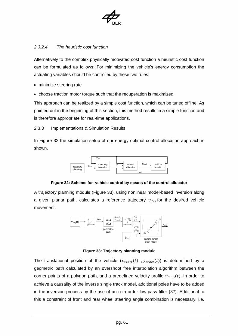
pg. 61
2.3.2.4 The heuristic cost function
Alternatively to the complex physically motivated cost function a heuristic cost function
can be formulated as follows: For minimizing the vehicle’s energy consumption the
actuating variables should be controlled by these two rules:
minimize steering rate
choose traction motor torque such that the recuperation is maximized.
This approach can be realized by a simple cost function, which can be tuned offline. As
pointed out in the beginning of this section, this method results in a simple function and
is therefore appropriate for real-time applications.
2.3.3 Implementations & Simulation Results
In Figure 32 the simulation setup of our energy optimal control allocation approach is
shown.
Figure 32: Scheme for vehicle control by means of the control allocator
A trajectory planning module (Figure 33), using nonlinear model-based inversion along
a given planar path, calculates a reference trajectory for the desired vehicle
movement.
Figure 33: Trajectory planning module
The translational position of the vehicle ( , ) is determined by a
geometric path calculated by an overshoot free interpolation algorithm between the
corner points of a polygon path, and a predefined velocity profile . In order to
achieve a causality of the inverse single track model, additional poles have to be added
in the inversion process by the use of an n-th order low-pass filter (37). Additional to
this a constraint of front and rear wheel steering angle combination is necessary, i.e.
control
allocator
trajectory
controller
vehicle
modeltrajectory
planning
vdes
vact
ucmd
uact
Δv
vlong(t)x(λ)
y(λ)t
PTn -1
inverse single
track model
λ(t)xexact(t)
yexact(t)
(t)y
(t)x
...
y(t)
x(t)
(n)
(n)
geometric
path
p(t)
vdes
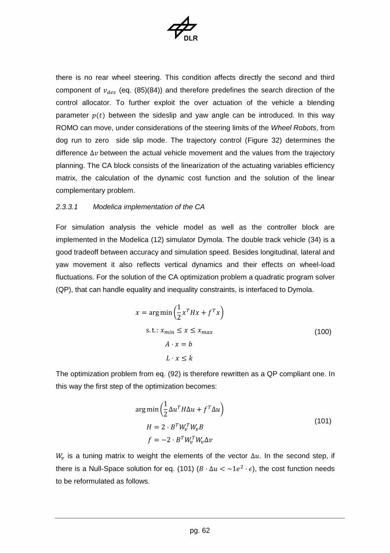
pg. 62
there is no rear wheel steering. This condition affects directly the second and third
component of (eq. (85)(84)) and therefore predefines the search direction of the
control allocator. To further exploit the over actuation of the vehicle a blending
parameter between the sideslip and yaw angle can be introduced. In this way
ROMO can move, under considerations of the steering limits of the Wheel Robots, from
dog run to zero side slip mode. The trajectory control (Figure 32) determines the
difference between the actual vehicle movement and the values from the trajectory
planning. The CA block consists of the linearization of the actuating variables efficiency
matrix, the calculation of the dynamic cost function and the solution of the linear
complementary problem.
2.3.3.1 Modelica implementation of the CA
For simulation analysis the vehicle model as well as the controller block are
implemented in the Modelica (12) simulator Dymola. The double track vehicle (34) is a
good tradeoff between accuracy and simulation speed. Besides longitudinal, lateral and
yaw movement it also reflects vertical dynamics and their effects on wheel-load
fluctuations. For the solution of the CA optimization problem a quadratic program solver
(QP), that can handle equality and inequality constraints, is interfaced to Dymola.
(
)
(100)
The optimization problem from eq. (92) is therefore rewritten as a QP compliant one. In
this way the first step of the optimization becomes:
(
)
(101)
is a tuning matrix to weight the elements of the vector . In the second step, if
there is a Null-Space solution for eq. (101) ( ), the cost function needs
to be reformulated as follows.

pg. 63
(102)
The physically motivated cost function, proposed in section 2.3.2.3, needs to be
approximated via a second order Taylor series expansion. The operating point needs
to be selected separately for the steering and the traction motor power. The steering
actuator power demand depends on the change of the steering angle, not on the angle
itself. Therefore, the expansion is chosen around the operating point from the last
calculated step ( in eq. (103)). On the contrary, the drive torque
operation point is set to the current time step ( in eq. (103)).
(
)
(
)
(103)
For the desired formulation as an optimization objective applicable to eq.(102), the
quadratic function of eq. (103) needs to be resorted.
The heuristic cost function (see 2.3.2.4) is considered as a weighted minimization
problem of the distance between the actuating variable and the demand . The
entries of the weighting matrix are the outcome of an offline closed loop
optimization with the DLR optimization software MOPS (23).
→
(104)
The rules of section 2.3.2.4 can be expressed with the actuating variation vector .
The steering rates are set to zero and the drive torque rates are set to the maximum
recuperation permitted by the current vehicle state.
( )
( )
(105)
2.3.3.2 Experimental setup and results
For the comparison of the different control strategies an ISO-double-lane-change
driving maneuver with predefined velocity profile is used (Figure 34). The focus of the

pg. 64
investigations is on a reproducible test. To achieve this, a lateral acceleration interval is
employed that does not reach the threshold of the tire and vehicle dynamics. The rear
steering of the inverse model in the trajectory planning module (Figure 33) in this
experiment is fixed. The car accelerates with up to time and then
changes volatile to .
Figure 34: ISO 3888-1 double lane change
This guaranties a considerable demand change especially to the traction motors to
highlight the potential of the CA optimization strategy.
Table 6: Overall energy consumption
Variant Energy consumption
Physically motivated cost function
Heuristic cost function
Both simulations with the physically motivated (section 2.3.2.3) and the heuristic
(section 2.3.2.4) cost function show almost identical results in the overall energy
consumption. Also the characteristics of the actuator variable commands differ only
negligibly and both of them generate feasible commands.
Figure 35: Actuating variables trajectory (solid = phys., dotted = heur.)
0 10 20 30 40 50 60 700
0.5
1
1.5
long.direction [m]
lat.
direction [
m]
Trajectory
0 2 4 6 8-0.1
-0.05
0
0.05
0.1
Steering angle [rad] front right
0 2 4 6 8
-5
0
5
x 10-3 Steering angle [rad] rear right
0 2 4 6 8
-100
0
100
200Drive torque [Nm] front right
0 2 4 6 8
-100
0
100
200Drive torque [Nm] rear right
time (s) time (s)

pg. 65
The computational complexity and necessity for a state observer to calculate the
physically motivated cost function calls its use in real-time applications into question.
For future developments the physically motivated cost function will be used as a
benchmark solution for real-time capable control algorithms. To capitalize on its
advantages these will be performed with true nonlinear optimization methods, like
SQP, in offline simulations.

pg. 66
3 Results
In conclusion we can say that all milestones of the work plan (compare Table 1) could
be fulfilled. The deliverables show that the chosen approach has a high potential and it
is worth to pursue them in the consecutive project FES III.
3.1 Conclusion and future work
It was shown that the technique of model based control design, which is very wide
spread in the field of robotics, can also be applied to energy optimal control for future
electric vehicle applications. By means of Kalman Filter based estimation algorithms in
combination with real-time capable prediction models, modelled in Modelica, the gap
between high accuracy and performance could be reduced tremendously. The given
simulation results, in combination with real experiment data, show the high potential of
the developed techniques. In future investigations, the focus will be on the transfer of
the algorithms to micro controller hardware on an experimental vehicle. In FES III the
focus will be on high level planning and optimization in combination with the coupling to
the vehicle and the driver.
3.2 Reflexion
The proposed approaches establish, due to their extension of freedom in vehicle
architecture design, a high potential for model based development in future automotive
controllers. Nevertheless the tool chains of the simulator developers and the code
generation process still have a lot of flaws to be user friendly enough to cleave towards
a wide spread in future controller development. Therefore projects like ITEA2
Modelisar, in which DLR RMC-SR also participates, can reduce this gap. Also the
developments in DLR FIZ, will support this. Finally we can say that through this
development we could derive a clear view were the open research points are and also
reflect them already to the new project plans in FES III and FIZ.
3.3 Accompanying third party projects
The robotic test platform ROboMObil, which also has been used here in this work
package for several investigations, was funded by BayStMWIVT within the project
“Wheel robots”. The developed models for the real-time application are now part of the
commercial Modelica Powertrain Library 2.1, which is distributed by Dassault Systems.

pg. 67
4 Publications & References
1. Krause, Paul C., Wasynczuk, Oleg and Sudhoff, Scott C. Analysis of electric
machinery and drive systems. New York : IEEE Press, 2002. Second Edition.
2. Wayne, Beaty H. and Kirtley, J.L. Electric Motor Handbook. New York : McGraw-
Hill, 1998.
3. Schröder, D. Elektrische Antriebe - Regelung von Antriebssystemen. Berlin
Heidelberg : Springer-Verlag, 2009. 3. Auflage.
4. Drury, Bill. The Control Techniques Drives and Control Handbook. London : The
Institute of Engineering and Technology, 2009. Second Edition.
5. Alaküla, Mats and Karlsson, Per. Power Electronics - Devices, Converters, Control
and Applications. Lund : Lunds University, 2009.
6. Hybrid-Autos.Info. [Online] [Cited: Juni 25, 2010.] http://www.hybrid-
autos.info/technik/e-maschinen/.
7. Ong, Chee-Mung. Dynamic Simulation of electric machinery. Upper Saddle River :
Prentice Hall, 1998.
8. Roshen, Waseen. Iron Loss Model for Permanent-Magnet Synchronous Motor.
Hilliard : IEEE Transactions on Magnetics, 2007. Vol. 43.
9. Herranz Gracia, M., Lange, E. and Hameyer, K. Numerical Calculation of Iron
Losses in Electrical Machines with a Modified Post-Processing Formula. Aachen :
Institute of Electrical Machines, RWTH Aachen University, 2007.
10. Semikron. IGBT- und MOSFET-Leistungsmodule. Nürnberg : s.n., 2010.
11. Schröder, D. Leistungselektronische Schaltungen. Berlin Heidelberg : Springer-
Verlag, 2008. 2. Auflage.
12. Association, Modelica. Modelica - A Unified Object-Oriented Language for
Physical Systems Modeling Language Specification Version 3.2. 2010.
13. ROMO – THE ROBOTIC ELECTRIC VEHICLE. Brembeck, J., et al., et al.
Manchester : s.n., 2011. 22nd IAVSD International Symposium on Dynamics of Vehicle
on Roads and Tracks.

pg. 68
14. Simon, D. Optimal State Estimation: Kalman, H Infinity, and Nonlinear Approaches.
1. Auflage. s.l. : Wiley & Sons, 2006.
15. Ljung, Lennart. System Identification: Theory for the User (2nd Edition). s.l. :
Prentice Hall PTR, 1998.
16. Sigma-Point Kalman Filters for Nonlinear Estimation and Sensor-Fusion:
Applications to Integrated Navigation. Merwe, R. van der, Wan, Eric and Julier,
Simon. 2004.
17. The square-root unscented Kalman filter for state and parameter-estimation.
Merwe, R. van der and Wan, E. A. 2001. Vol. 6, pp. 3461-3464 vol.6.
18. High-performance battery-pack power estimation using a dynamic cell model. Plett,
G.L. 5, 2004, Vehicular Technology, IEEE Transactions on, Vol. 53, pp. 1586-1593.
19. Extended Kalman filtering for battery management systems of LiPB-based HEV
battery packs: Part 1. Background. Plett, Gregory L. 2, 2004, Journal of Power
Sources, Vol. 134, pp. 252-261.
20. Extended Kalman filtering for battery management systems of LiPB-based HEV
battery packs: Part 2. Modeling and identification. Plett, Gregory L. 2, 2004, Journal of
Power Sources, Vol. 134, pp. 262-276.
21. Extended Kalman filtering for battery management systems of LiPB-based HEV
battery packs: Part 3. State and parameter estimation. Plett, Gregory L. 2, 2004,
Journal of Power Sources, Vol. 134, pp. 277-292.
22. Graaf, Roger. Simulation hybrider Antriebskonzepte mit Kurzzeitspeicher für
Kraftfahrzeuge. Ika RWTH, Aachen. 2010.
23. A multiobjective optimisation-based software environment for control systems
design. Joos, H.-D. Glasgow : s.n., 2002. 12th IEEE International Symposium on
Computer Aided Control System Design. pp. 7-14. ISSN: DOI:
10.1109/CACSD.2002.1036921.
24. Wielgos, Sebastian, et al., et al. Development of an Energy Management System
for Electric Vehicles Design and System Simulation. Technische Universität München.
2010.
25. Engst, Christian, et al., et al. Object-Oriented Modelling and Real-Time
Simulation of an Electric Vehicle in Modelica. Technische Universität München. 2010.
pg. 69
26. The ARTEMIS European driving cycles for measuring car pollutant emissions.
André, Michel. 2004, Science of The Total Environment, Vols. 334-335, pp. 73-84.
Highway and Urban Pollution.
27. Human Machine Interface Concept for Interactive Motion Control of a Highly
Maneuverable Robotic Vehicle. Bünte, T., Brembeck, J. and Ho, L. M. Baden Baden :
s.n., 2011. Intelligent Vehicles Symposium (IV), IEEE. pp. 1170 - 1175. ISSN: 1931-
0587 DOI: 10.1109/IVS.2011.5940490.
28. Applying Management Methodology to Electric Vehicles with Multiple Energy
Storage Systems. Rosario, L. and Luk, P.C.K. Hong Kong : s.n., 2007. International
Conference on Machine Learning and Cybernetics. Vol. 7, pp. 4223-4230.
29. Brembeck, J. and Ritzer, P. Energie- und Leistungsmanagement in
Elektrofahrzeugen. DLR Robotics and Mechatronics Center. Oberpfaffenhofen : s.n.,
2012. Internal Report. Internal Report.
30. Selectively Damped Least Squares for Inverse Kinematics. Buss, S. R. and Kim,
J.-S. 3, University of California, San Diego : s.n., 2004, Journal of Graphics Tools, Vol.
10, pp. 37-49.
31. Härkegard, O. Backstepping and Control Allocation with Applications to Flight
Control. Linköping University, Department of Electrical Engineering. Linköping
University, Sweden : s.n., 2003. Ph.D. Dissertation. Author of QCAT.
32. Coordination of Vehicle Motion and Energy Management Control Systems for
Wheel Motor Driven Vehicles. Laine, L. and Fredriksson, J. Istanbul : s.n., 2007.
Intelligent Vehicles Symposium (IV), IEEE. pp. 773-780. ISSN: 1931-0587 DOI:
10.1109/IVS.2007.4290210.
33. Optimized Force Allocation - A General Approach to Control and to Investigate the
Motion of Over-Actuated Vehicles. Knobel, C., Pruckner, A. and Bünte, T.
Heidelberg : s.n., 2006. 4th IFAC Symposium on Mechatronic Systems. pp. 366-371.
34. Orend, R. Integrierte Fahrdynamikregelung mit Einzelradaktorik. Technischen
Fakultät der Universität Erlangen-Nürnberg. 2006. Dissertation.
35. Beck, R. E. Application of Control Allocation Methods to Linear Systems with Four
or More Objectives. Virginia Polytechnic Institute and State University. USA : s.n.,
2002. Ph.D. Dissertation.

pg. 70
36. Buss, S. R. and Kim, J.-S. Introduction to Inverse Kinematics with Jacobian
Transpose, Pseudoinverse and Damped Least Squares methods. Department of
Mathematics. University of California, San Diego : s.n., 2004. This is an introduction
that was originally written for a paper by.
37. Nonlinear Inverse Models for Control. Thummel, M., et al., et al. Hamburg : s.n.,
2005. 4th International Modelica Conference. pp. 267-279.
38. Research on thermo-physical properties identification and thermal analysis of EV
Li-ion battery. Cheng, Lin, et al., et al. 2009. pp. 1643-1648.
39. Advanced Electro-Thermal Modeling of Lithium-Ion Battery System for Hybrid
Electric Vehicle Applications. Mi, C., et al., et al. 2007. pp. 107-111.
40. Construction of three-dimensional thermal simulation model of lithium-ion
secondary battery. Matsushita, T., et al., et al. 2008. pp. 1-6.
41. Constrained state estimation using the Unscented Kalman Filter. Kandepu, R.,
Imsland, L. and Foss, B.A. 2008. pp. 1453-1458.
42. Incorporation of time delayed measurements in a discrete-time Kalman filter.
Larsen, T. D., et al., et al. 1998. Vol. 4, pp. 3972-3977.
43. Engst, C., Brembeck, J. and Kennel, R. Object-Oriented Modelling and Real-
Time Simulation of an Electric Vehicle in Modelica. TUM. Munich : s.n., 2010. Master
Thesis.
44. Simon, D. Kalman filtering with state constraints: a survey of linear and nonlinear
algorithms. s.l. : IET Control Theory & Applications, 2010. p. 1303+.
45. Jonasson, Mat. Aspects of Autonomous Corner Modules as an Enabler for New
Vehicle Chassis Solutions. Royal Institute of Technology. Stockholm : s.n., 2007.
Licentiate Thesis.
http://www.google.de/url?sa=t&source=web&cd=1&ved=0CBwQFjAA&url=http%3A%2
F%2Fwww.diva-
portal.org%2Fsmash%2Fget%2Fdiva2%3A11577%2FFULLTEXT01&ei=-
iwtTpG4B4ee-Qa3v-HsDQ&usg=AFQjCNE73f2gChTnVeBqdPm1Zvwv2Ug88w.
46. Development of the ExoMars Chassis and Locomotion Subsystem. Michaud, S, et
al., et al. Los Angeles, California : s.n., 2008. 9th International Symposium on Artificial
Intelligence, Robotics and Automation in Space, iSairas '08.

pg. 71
47. Robotic Electric Vehicle with Camera-based Autonomy Approach. Schaub,
Alexander, et al., et al. 2, 2011, ATZelektronik, Vol. 2, pp. 10-16.
48. Asogawa, Katsunori. Variable Wheel Positioning in a Vehicle. EP1902926 03 26,
2008.
49. Gashi, Rexhep and Laurent, Daniel. Vehicle ground connection comprising a
wheel and a suspension. US2008/0100020 05 01, 2008.
50. Siemens VDO announces eCorner motor-in-hub concept. [Online] 08 10, 2006.
[Cited: 07 25, 2011.] http://www.autoblog.com/2006/08/10/siemens-vdo-announces-
ecorner-motor-in-hub-concept/.
51. Machbarkeitstudie zur Entwicklung eines eCorners. DLR. Wessling : s.n., 2009.
52. A real time capable battery model for electric mobility applications using optimal
estimation methods. Brembeck, Jonathan and Wielgos, Sebastian. Dresden,
Germany : s.n., 2011. Proceedings 8th Modelica Conference. pp. 398-405.
53. ISO 7401, Road vehicles; laterial transient response test methods. 1988.
54. Schmitt, Peter. Just build it! : a fully functional concept vehicle using robotic
wheels. s.l. : Massachusetts Institute of Technology, School of Architecture and
Planning, Program in Media Arts and Sciences, 2007. Thesis (S.M.).
55. Better Place. [Online] 2011. [Cited: 07 2011, 27.] http://www.betterplace.com.
56. Dynamic Simulation of a Free-Piston Linear Alternator in Modelica. Pohl, S.E. and
Gräf, M. Hamburg, Germany : s.n., 2005. Proceedings of the 4th International Modelica
Conference.
57. Hartweg, Stefan. Master Thesis: Einfluss elastischer Strukturen auf
Fahrdynamikregelysteme. s.l. : Institut für Kraftfahrzeuge (IKA), RWTH Aachen, 2010.
58. Human machine interface concept for interactive motion control of a highly
maneuverable robotic vehicle. Bünte, Tilman, Brembeck, Jonathan and Ho, Lok
Man. Baden-Baden, Germany : s.n., 2011. IEEE Intelligent Vehicles Symposium (IV).
pp. 1170-1175.
59. Stereo Processing by Semiglobal Matching and Mutual Information. Hirschmüller,
H. 2, 2008, Pattern Analysis and Machine Intelligence, IEEE Transactions on, Vol. 30,
pp. 328-341.

pg. 72
60. Optimized Force Allocation - A General Approach to Control and to Investigate the
Motion of Over-Actuated Vehicles. Knobel, Christian, Pruckner, Alfred and Bünte,
Tilman. Heidelberg : s.n., 2006. 4th IFAC Symposium on Mechatronic Systems. Vol.
Volume 44.