faculty of engineering vol. 44 no. july 2016 pp. 362 ... · 353 jes, assiut university, faculty of...

351

Journal of Engineering Sciences

Assiut University

Faculty of Engineering

Vol. 44

No. 4

July 2016

PP. 351 – 362

* Corresponding author.

E- mail address: [email protected]

SIMPLIFICATION OF WATER SUPPLY SYSTEMS FOR

PRODUCING MORE OPTIMAL PUMP SCHEDULES IN LESS TIMES

Nashat A. Ali, Gamal Abozeid, Moustafa S. Darweesh and Mohamed Mamdouh *

Staff in Civil Eng Dept, Faculty of Engineering, Assuit Univ, 71516 Assuit.

Received 23 March 2016; Accepted 25 June 2016

ABSTRACT

Simplification of large water supply networks is used for reducing computation times and for

making it easier to manage, monitor and analyze. The effect of networks’ simplification on raising

the efficiency of pump optimization process is investigated. The key topic of this paper is to

produce more optimal pump schedules by using simplified networks. In this research, twelve of

demand allocation methods are used after the simplification process and the best one is selected.

Then, the simplified network is used for finding a better pump schedule than that produced from the

original one under the same conditions, by using Genetic Algorithm (GA) in WaterGEMS V8i

software. The produced schedule from the simplified network is applied on the original network to

check its performance. Two examples are studied. First, Scheduler Sample1 is reduced by 52 % for

pipes and 50 % of nodes. The schedule produced from the simplified network, after applying it on

the original network, gives a better solution than that produced from the original one by 9 % in the

energy cost along a week and by 12 % in the time for optimization. Second, New El- Minia city

network is simplified by removing 82 % from its pipes and 77 % of its nodes. The schedule

produced from the simplified network saves the energy consumption along a week by 1.7 % and the

time for optimization by 74 % after applying it on the original network.

Keywords: Pump optimization, pipes network, simplification, demand allocation.

1. Introduction

Modeling of a hydraulic system is a main issue, and it is not always convenient to model

every component in the network. Skeletonization of the network to a simplified one reduces its

complexity for calibration, operation and monitoring purposes. However, the level of

skeletonization used depends on the intended use of the model (Lamoudi et al. [7]). Maschler

& Savic [8] specified two main ways to simplify a network model, which are simplification of

network model components and black box simplification. Mohamed and Ahmed [9] used the

first way in three levels to study the effect of network simplification on the chlorine

distribution. They found that increasing network simplification could effectively increase the

error in water quality modeling. Gad and Mohamed [4] simplified a network by using the first

352

Mohamed Mamdouh et al., Simplification of water supply systems for producing more optimal …….

way in three levels and the impact of network’s simplification on water hammer phenomenon

was investigated. They found that increasing of simplification degree gave inaccurate transient

pressure results. Moser and Smith [11] simplified a network by using the second way. They

combined a strategy of model falsification with network reduction techniques to obtain reliable

and efficient diagnoses. They found that this methodology had a potential to detect leak

regions; even with a small number of sensors. Preis et al. [13] used the second way to reduce a

network by 93% of its pipes and 97% of its nodes. They used the simplified model with

statistical data-driven algorithm and GA to estimate future water demands. The simplified

model reduced the computation time by 89%. Paluszczyszyn et al. [12] used the second way to

present an online simplification algorithm, which can be used to manage abnormal situations,

and structural changes to a network, e.g. isolation of part of a network that due to a pipe burst.

This approach allowed preserving the hydraulic and energetic characteristics of the original

water network. Skworcow et al. [15] used the previous approach for reducing the network,

while maintaining the energy distribution in the simplified network. The simplified network

was used for minimizing the energy cost and leakage, while achieving operational constraints.

Georgescu and Georgescu [5] reduced a real network by using a numerical network model and

data recorded. By using the Honey Bees Mating Optimization Algorithm (HBMOA), they

could save about 32% of daily energy consumption.

Many researchers harnessed GA for finding optimal pump schedules. Moreira and Ramos

[10] reduced the daily energy cost of a real network by 43.7%, by using GA with a manual

override approach. Behandish and Wu [2] used the Artificial Neural Network (ANN) with

GA to reduce the daily energy cost of a real system by about 10-15%. Amirabdollahian and

Mokhtari [1] utilized fuzzy genetic algorithm with uncertain hydraulic constraints to

determine siting and sizing of tanks and pumps. They concluded that this approach reduced

the computational costs and improved the network performance. Puleo et al. [14] coupled

linear programming with GA. The proposed hybrid optimization model dominated on the

traditional metaheuristic algorithms in terms of rapid convergence and reliability. Blinco et

al. [3] developed a GA model to solve multi objectives pumping operation problem. The

objectives were reducing cost, energy and Green House Gas emissions (GHG). They

developed an interface, which allows users to employ this approach to their networks.

According to the above literature, simplification of water pipes network has been utilized

for various aspects related to water distribution systems. Despite the enormous computational

power available in these days, the requirements of water distribution systems become more

complex and complicated in terms of size, objectives, and constraints. So, there is an ongoing

seek for techniques or algorithms that can rapidly identify feasible solutions.

This study aim to investigate the effect of water networks simplification on pump

optimization process to find better solutions in fewer times under the same hydraulic

conditions and GA characteristics.

2. Theoretical considerations The pump scheduling problem is treated as a single objective optimization problem subjected

to some constraints. The objective function is given as follows (Giacomello et al. [6]);

(1)

353

JES, Assiut University, Faculty of Engineering, Vol. 44, No. 3, July 2016, pp. 351– 362

Where T = number of hydraulic time steps during the operating period; NPumps =

number of active pumps in the pump station; γ = specific weight of water; CP,T = cost of

electricity (in pecuniary units per KWh) during time t at pump station p; ηp = overall

efficiency of pump p; Qp,t = discharge of pump p during time t; Hp,t = acting head of pump

p during time t; and Δt = hydraulic time step (typically 1 hr).

This objective is restricted by physical and operational constraints. Physical constraints

describe the hydraulic behavior of the network (conservation of mass and energy), while

operational constraints are identified by the utility throughout the network to meet its needs.

The conservation of mass at junctions is defined as follows;

Where Qij,t = discharge in pipe ij at time t; and qi,t = demand at junction i at time t. Mass

balance in tanks can be illustrated with the following equation;

Where Si = cross-sectional area of tank i (assuming cylindrical tank); Yi,t = water elevation

in tank at time t; Yi,t − Δt = water elevation at previous time step; and Yi,0= The water elevation

in tank i at the beginning of the operating period. Both Eqs. (2) and (3) are written for every

junction at each time t. The conservation of energy equation is introduced as follows;

Where Hi,t and Hj,t = heads in starting and ending junctions of pipe ij at time t; Rij =

resistance coefficient for pipe ij; and n = exponent of discharge term.

factor when water enters a centrifugal pump p is defined as follows;

Where Ap and Bp = two resistance coefficients; and Cp = shutoff head. Both Eqs. (4) and

(5) are written for every pipe ij and every pump p at each time t.

The operational constraints usually contain restrictions on nodal pressures, tank levels,

and boundary conditions. Firstly, pressure constraint which means that the pressure should be

above some minimum required value, Hreq

i,t , for each hydraulic time step t at each node;

If necessary, a maximum value of nodal pressure could also be added. In addition, the minimum

and maximum water levels at all tanks must be constrained for each hydraulic time step t;

(2)

(3)

(4)

(5)

(6)

354


Where Ymin

i and Ymax

i = minimum and maximum water levels in tank i. In addition to that,

each tank has to be operated in a way to ensure that the water level inside tank i at the end of

the day, Yi,T, is more than that at the beginning of that day, Yi,0. This leads to reassure that tank

balance will be achieved in the following day. This constraint can be expressed as follows;

The operational constraints also contained velocity limitations which are;

Vmin ≤ Vij,t

Vij,t ≤ Vmax

Where Vij,t = water velocity of pipe ij at time t, Vmin

and Vmax

= minimum and maximum

water velocities in the pipe.

Furthermore, it is possible to calculate the search space of the pump optimization

problems. If you have Np of pumps, Ns of pump speed settings and Hs of hydraulic time

steps in your duration time, the search space is S = Ns^ ( Np * Hs).

3. Case study Two examples are given in this study to illustrate the benefit of the network

simplification in the pump optimization process.

1- Example 1: Scheduler Sample 1

SchedulerSample1 is a municipal water distribution network available in WaterCAD

User’s Guide [16] as shown in Fig. 1. This network contains 554 pipes and 458 nodes with

looped and branch system. There is one source of water feeding the network with fixed

water level = 184 m, and a circular elevated tank of 14 m diameter with a height of 27 m as

shown in Fig. 1. The initial tank level is 17.37 m at the beginning of the simulation time

(24 hours). The network has a pump station containing 5 pumps and the total average daily

demand is 93 L/s. Elevations of the network nodes, average base demands for the different

nodes and time demand pattern are considered. The distribution system composes of

95,432.00 m of different diameter pipelines. All of them are ductile iron, and the head loss

in each pipe is computed using Hazen-Williams formula. In addition to that, Fig. 2 shows

the day hours when pumps are turned off and turned on in this network.

Fig. 1. Schedulersample1 network (the original network).

(7)

(8)

(9)

(10)

(11)

355


Fig. 2. The pump schedules of the Schedulersample1original network.

2- Example 2: New El- Minia city network

New El- Minia city is located about 250 km south of Cairo on the eastern bank of the

River Nile, and has a drinking water distribution network as shown in Fig. 3. This network

consists of 1348 pipes and 943 nodes, and there is one source of water feeding the network

with water level = 150.96 m. This network has a circular elevated tank of 19.4 m diameter

with a height of 62 m, and the total average daily demand is 170.7 L/s. Elevations of the

network junctions, average base demands for the different junctions and time demand

pattern are taken into consideration. The distribution system composes of 188 Km of

different diameter pipelines of Poly Vinyl Chloride (PVC), and the head loss in each pipe

is computed using Hazen-Williams formula. Furthermore, Fig. 4 depicts that the pump

station is working for 24 hours daily.

Fig. 3. New El- Minia city network (the original network).

Fig. 4. The pump schedule of New El- Minia city network before optimization.

4. Methodology

First of all, simplification of network model components method, which includes

deletion of trees, removal of small diameter pipes and trimming of short pipe segments

including dead nodes (with no or little demand), is used intuitively to simplify water pipes

network to make it easier for both analyzing and optimizing. Secondly, twelve of demand

allocation methods (available in WaterGEMS V8i software) are used to redistribute the

demands of the removed nodes to the simplified network, and the best method is selected

356


to give the closest picture to the original network. For reducing the energy consumed by

the pump station while achieving the physical and operational constraints, pump

scheduling optimization is accomplished by using both the original network (without

simplification) and the simplified one (with the best demand allocation method), with the

same constraints and GA options in Darwin Scheduler (a tool in WaterGEMS V8i).

Finally, a comparison between the performance of schedules, produced from the original

and the simplified network has been done within the original network, to explore the effect

of network simplification on facilitating the pump optimization process, in terms of

percentage of saved energy and time taken for optimization.

5. Results and discussions

5.1. Simplification process

We adopt simplification of network model components procedure to reduce our networks.

Deletion of trees, removal of small diameter pipes and trimming of short pipe segments

including dead nodes (with no or little demand) are some techniques in this procedure. These

techniques are used to skeletonize the studied networks. This kind of simplification does not

contain any changes in pump stations or tanks. Schedulersample1 original network is

reduced, from 554 pipes to 264 pipes (52%) and from 458 nodes to 231 nodes (50%), and

shown in Fig. 5. New El- Minia city original network is reduced, from 1348 pipes to 243

pipes (82%) and from 943 nodes to 221 nodes (77%), and depicted in Fig. 6.

Fig. 5. Scheduler sample 1 network (the simplified network).

Fig. 6. New El- Minia city network (the simplified network).

Twelve of demand allocation methods, some of them are available in WaterCAD User’s

Guide [16], are used to reallocate the demands of the removed nodes to the simplified

network. The best method is that produces flows in the pipes of the simplified network

very close to flows in its corresponding pipes in the original network. These methods and

their index values are listed in Table (1).

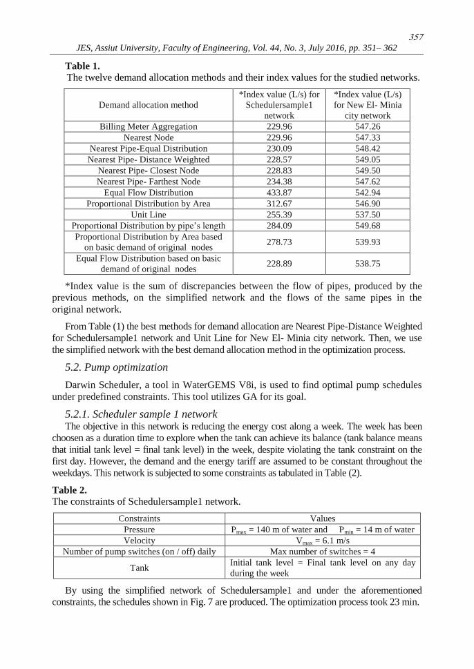
357


Table 1.

The twelve demand allocation methods and their index values for the studied networks.

Demand allocation method

*Index value (L/s) for

Schedulersample1

network

*Index value (L/s)

for New El- Minia

city network

Billing Meter Aggregation 229.96 547.26

Nearest Node 229.96 547.33

Nearest Pipe-Equal Distribution 230.09 548.42

Nearest Pipe- Distance Weighted 228.57 549.05

Nearest Pipe- Closest Node 228.83 549.50

Nearest Pipe- Farthest Node 234.38 547.62

Equal Flow Distribution 433.87 542.94

Proportional Distribution by Area 312.67 546.90

Unit Line 255.39 537.50

Proportional Distribution by pipe’s length 284.09 549.68

Proportional Distribution by Area based

on basic demand of original nodes 278.73 539.93

Equal Flow Distribution based on basic

demand of original nodes 228.89 538.75

*Index value is the sum of discrepancies between the flow of pipes, produced by the

previous methods, on the simplified network and the flows of the same pipes in the

original network.

From Table (1) the best methods for demand allocation are Nearest Pipe-Distance Weighted

for Schedulersample1 network and Unit Line for New El- Minia city network. Then, we use

the simplified network with the best demand allocation method in the optimization process.

5.2. Pump optimization

Darwin Scheduler, a tool in WaterGEMS V8i, is used to find optimal pump schedules

under predefined constraints. This tool utilizes GA for its goal.

5.2.1. Scheduler sample 1 network The objective in this network is reducing the energy cost along a week. The week has been

choosen as a duration time to explore when the tank can achieve its balance (tank balance means

that initial tank level = final tank level) in the week, despite violating the tank constraint on the

first day. However, the demand and the energy tariff are assumed to be constant throughout the

weekdays. This network is subjected to some constraints as tabulated in Table (2).

Table 2.

The constraints of Schedulersample1 network.

Constraints Values

Pressure Pmax = 140 m of water and Pmin = 14 m of water

Velocity Vmax = 6.1 m/s

Number of pump switches (on / off) daily Max number of switches = 4

Tank Initial tank level = Final tank level on any day

during the week

By using the simplified network of Schedulersample1 and under the aforementioned

constraints, the schedules shown in Fig. 7 are produced. The optimization process took 23 min.

358


Fig. 7. The pump schedules produced from the Schedulersample1simplified network.

The optimization process is repeated with the original network of Schedulersample1

under the same constraints and the same GA options. The produced schedules are

presented in Fig. 8. It is observed that the optimization process was achieved in 26 min

with an increase of 11.5% compared to the simplified network.

Fig. 8. The produced optimized schedules from the Schedulersample1original network.

In Table (3), a comparison between the previous schedules (Figs. 5, 6 and 7) are made

by applying them to the original network with full tank level on the first day of the week.

Table 3.

The performance of the previous schedules along a week.

Schedules Energy cost

($/week)

Pressure

constraint

Velocity

constraint Tank constraint

Figure 7 1088 No

violation

No

violation

Tank balance is achieved on the

second day with 15.28 m

Figure 8 1190 No

violation

No

violation

Tank balance is achieved on the first

day with 17.37 m

Figure 2 1231 No

violation

No

violation

Tank balance is achieved on the

third day with 12.51 m

From Table (3), it is obvious that the energy cost of the schedules produced from the

simplified network in Fig. 7 is less than the energy cost of the schedules produced from the

original network in Fig. 8 by 9%. In addition, the time taken to produce the schedules in

Fig. 7 is less than the elapsed time to create the schedules in Fig. 6 by 11.5%. On the other

hand, pump 3 in the schedules produced from the simplified network in Fig. 7 has six

switches per day which violate the number of pump switches constraint.

5.2.2. New El- Minia city network Reducing the energy consumption is the objective in this network while achieving the

constraint as listed in Table (4).

359


Table 4.

The constraints of New El- Minia city network.

Constraints Values

Pressure Pmin = 30 m of water

Velocity Vmax = 2 m/s

Number of pump switches

(on / off) daily Max number of switches = 4

Tank Initial tank level = Final tank level on any day

during the week

The optimization of the simplified network of New El- Minia City with the constraint

presented in Table (4) produces the schedule as shown in Fig. 9 in 17 min. However, the

optimization process under the same constraints and GA options when repeated with the

original network of New El- Minia City, the schedule in Fig. 10 is produced in 66 min.

Fig. 9. The pump schedule of New El- Minia city simplified network.

Fig. 10. The pump schedule of New El- Minia city original network.

The difference between the obtained schedules in Figs. 4, 9 and 10 is summarized in

Table (5). The schedules are applied on the original network with 0.15 m as the initial tank

level on the first day in the week.

Table 5.

The performance of New El- Minia City schedules of Figures 8,9 and 10 along a week.

Schedules

Energy

consumption

(kwh/week)

Pressure

constraint

Velocity

constraint Tank constraint

Figure 9 22526 No violation No violation Tank balance is achieved on the

second day with 1.58 m.


fourth day with 7.75 m.


second day with 10.15 m.

From Table (5), it is obvious that the energy consumption of the schedule produced

from the simplified network in Fig. 9 is less than the energy consumption of the schedule

produced from the original network in Fig. 10 by 1.8 %. In addition, the time taken to

produce the schedule in Fig. 9 is less than the elapsed time to create the schedule in Fig. 10

by 74 %. Also, the schedule produced from the simplified network in Fig. 9 achieves the

pump switches constraint unlike the schedule in Fig. 10 which violates this constraint by

eight switches per day. On the other hand, Figure 4 shows the schedule of New El- Minia

City network before optimization without any stops leading to a higher energy

consumption compared to that of the optimized simplified network.

360


Finally, Table (6) clarifies the effect of network simplification on facilitating the pump

optimization process in terms of producing pump schedules with less energy consumption

and take minimal time for optimizing. In terms of reducing the time taken for optimization,

simplification of Schedulersample1 network by 51% in average has led to 11.5% save in

time, and about 74% has been reduced after simplification of New El- Minia city network by

80%. These percentages can be supported by the view that the software can deal with a

simplified network easier than a complex one, especially when it comes to optimization

problems which require a lot of iterations to find the optimum solution. So, the more the

network is simplified, the less optimization time it will take. However, the remarkable

difference, in decline of the optimization time between the two examples, is due to the

difference in number of pumps in each example. By this I mean that, the first example has

five pumps with size of search space equals 2^(5*24), but the second one has only one pump

with 2^(1*24) search space size. Consequently, the bigger the search space you may have,

the more time it will be taken for optimization. Owing to the fact that, New El- Minia city

network has started its lifetime recently, with demand equals only 170.7 L/s (around 145.41

L/s go to the surrounding villages), the percentages of saved energy are not sensible enough,

and subsequently the saved energy in the first case is 5 times higher than that in this network.

Table 6.

Comparison between saved energy and optimization time for the original and simplified

networks of the two case studies.

Example Network Simplification

Optimized

pump

schedules

Time for

optimizing

(min)

Saved

percentage

Schedulersample1

network

Original No No

Original No Yes 26 3.33%

Simplified Yes Yes 23 11.62%

New El- Minia city

network

Original No No

Original No Yes 66 0.65%

Simplified Yes Yes 17 2.36%

6. Conclusions

Simplification of network model components technique is used to skeletonize water

distribution networks. Twelve of demand allocation methods are utilized to preserve that the

overall system demand is kept unchanged in the reduced model. The best one is selected and

used for finding optimal pump schedule. A comparison between this schedule and that

produced from the original network after applying them on the original network is made.

Although, the studied simplification technique doesn’t reduce the search space S. However,

the time elapsed in the optimization process is reduced by 12% in example 1 and significantly

by 74% in example 2. Also, pump scheduling, created by using the simplified network, resulted

in energy savings of 9% in example 1 and 1.7% in example 2, when compared to schedule,

created by using the original network, with the same GA characteristics.

It is recommended that any suggested simplification technique used for pump optimization

process should preserve both hydraulic and energy characteristics of the original network.

Otherwise, the proposed schedules must be checked within the original network.

361


REFERENCES

[1] Amirabdollahian, M. and Mokhtari, M., “Optimal design of pumped water distribution

networks with storage under uncertain hydraulic constraints”, J. of Water Resour. Manage.,

Vol. 29, Issue 8, pp. 2637-2653, (2015).

[2] Behandish, M. and Wu, Z. Y., “Concurrent pump scheduling and storage level

optimization using meta-models and evolutionary algorithms”, 12th

Int. Conf. on

Computing and Control for the Water Industry, CCWI, Vol. 70, pp. 103–112, (2014).

[3] Blinco, L. J., Simpson, A. R., Lambert, M. F., Auricht, C. A., Hurr, N. E., Tiggemann, S. M.

and Marchi, A. “Genetic algorithm optimization of operational costs and greenhouse gas

emissions for water distribution systems”, 16th Water Distribution System Analysis Conf.,

WDSA- Urban Water Hydroinformatics and Strategic Planning, Vol. 89, pp. 509–516, (2014).

[4] Gad, A. A. M. and Mohamed, H. I., “Impact of pipes networks simplification on water

hammer phenomenon”, Sadhana j., Vol. 39, Issue 5, pp. 1227-1244, (2014).

[5] Georgescu, S. C. and Georgescu, A. M., “Application of HBMOA to pumping stations

scheduling for a water distribution network with multiple tanks”, 12th

Int. Conf. on

Computing and Control for the Water Industry, CCWI, Vol. 70, pp. 715–723, (2014).

[6] Giacomello, C., Kapelan, Z. and Nicolini, M., “Fast hybrid optimization method for effective

pump scheduling”, J. Water Resour. Plann. Manage, Vol. 139, Issue 2, pp. 175-183, (2013).

[7] Lamoudi, K. B., Bergerand, J. L. and Carrier, F., “Automated simplification of water

networks models”, Internship report – Master 2 CCI, (2013).

[8] Maschler, T. and Savic, D. A., “Simplification of water supply network models through

linearization”, Centre for Water Systems, Exeter University, Report No.99 (1), pp. 1-119, (1999).

[9] Mohamed, H. I. and Ahmed, S. S., “Effect of simplifying the water supply pipe networks on water

quality simulation”, Inter. Conf. for Water, Energy Environ., Sharijah, UAE, pp. 41–46, (2011).

[10] Moreira, D. F. and Ramos, H. M., “Energy cost optimization in a water supply system case

study”, J. of Energy. Vol. 2013, pp. 1-9, (2013).

[11] Moser, G. and Smith, I. F. C., “Detecting leak regions through model falsification”, 20th

Int. Workshop: Intelligent Computing in Engineering, Vienna, Austria, Jully 1-3, (2013).

[12] Paluszczyszyn, D., Skworcow, P. and Ulanicki, B., “Online simplification of water

distribution network models for optimal scheduling”, J. Hydroinformatics, (2013).

[13] Preis, A., Whittle, A. J., Asce, m., Ostfeld, A. and Perelman, L., “Efficient hydraulic state

estimation technique using reduced models of urban water networks”, J. Water Resour.

Plann. Manage., Vol. 137, Issue 4, pp. 343–351, (2011).

[14] Puleo, V., Morley, M., Freni, G. and Savic, D. A., “A hybrid optimization method for real-time

pump-scheduling”, 11th Int. Conf. on Hydroinformatics - HIC2014, New York, USA, (2014).

[15] Skworcow, P., Paluszczyszyn, D., Ulanicki, B., Rudek, R. and Belrain, T., “Optimization

of pump and valve schedules in complex large-scale water distribution systems using

GAMS modeling language”, 12th

Int. Conf. on Computing and Control for the Water

Industry, CCWI, Vol. 70, pp. 1566–1574, (2014).

[16] WaterCAD User’s Guide: Water Distribution Modeling Software, Series 4, (2013).

362


" إستخدام تبسيط شبكات ٳمداد المياه في إنتاج جداول لتشغيل الطلمبات لخفض

ٳستهالكها من الطاقة الكهربية و في أوقات حسابية أقل "

الملخص العربى

خطوة أساسية في عملية تصميم هذه الشبكات. فعلى ،يعد تبسيط وإختصار شبكات اٳلمداد بمياه الشرب

يعطي صورة أقرب ما تكون إلى الواقع إال أنه من الممكن الرغم من أن تمثيل شبكة المي اه بأكملها حاسوبيا

لتقليل الوقت التغاضي عن تمثيل بعض مكونات الشبكة األقل أهمية و ذلك بهدف جعلها أقل تعقيدا و أيضا

ظرا االزم لحساب الخصائص الهيدروليكية الخاصة بشبكات المياه مثل الضغوط و السرعات و غيرها. و ن

تقوم شركات المياه ،ٳلرتفاع تكاليف الطاقة الكهربية المستهلكة لرفع المياه في منظومة اإلمداد بمياه الشرب

،خالل اليوم هذه الجداول تتضمن ساعات عمل كل طلمبة و ساعات توقفها ،بعمل جداول لتشغيل الطلمبات

لمياه المطلوب استهالكها و أيضا الضغوط بهدف تخفيض ٳستهالكها من الطاقة الكهربية و الوفاء بكميات ا

الالزمة لتوصيلها. يوجد العديد من الدراسات التي تناولت موضوع تخفيض الطاقة الكهربية باقتراح جداول

هذه الدراسات ٳستخدمت خوارزميات رياضية متعددة باإلضافة الى تبسيط الشبكة لتحقيق ،لتشغيل الطلمبات

أقل. هذا الهدف و في أوقات حسابية

و لذلك كان الغرض من هذه الدراسة:

تبسيط شبكات المياه و ٳعادة توزيع إستهالك المياه فيها بٳستخدام اثني عشر طريقة مختلفة و إختيار .1

الطريقة األفضل.

في إنتاج جداول لتشغيل ،بعد إعادة توزيع اٳلستهالك بأفضل طريقة،ٳستخدام الشبكة المبسطة .2

الكهربية.الطلمبات لخفض الطاقة

المقارنة بين جداول تشغيل الطلمبات التي تم ٳنتاجها بإستخدام الشبكة المبسطة و جداول تشغيل .3

للوقوف على دور تبسيط الشبكات ،الطلمبات التي تم ٳنتاجها بإستخدام الشبكة األصلية بدون تبسيط

في ٳنتاج جداول تشغيل للطلمبات تستهلك طاقة كهربية أقل.

. يحتوي هذا البرنامج على Bentley WaterGEMS V8iحث دراسة نظرية بإستخدام برنامج يقدم هذا الب

و هي أداة Darwin Schedulerعدة طرق لتوزيع ٳستهالك المياه بعد تبسيط الشبكة و أيضا يحتوي على

إحداهما ،في إنتاج جداول تشغيل الطلمبات. تم ٳستخدام شبكتين للمياه Genetic Algorithm (GA)تستخدم

و ،شبكة موجودة في أمثلة هذا البرنامج و األخرى شبكة حقيقية هي شبكة مياه الشرب بمدينة المنيا الجديدة

ذلك لبيان دور تبسيط الشبكة في ٳنتاج جداول تشغيل للطلمبات تستهلك طاقة أقل و في أوقات حسابية أقل. كان

من أهم النتائج المستخلصة من هذا البحث اآلتي:

مكن إنتاج جداول تشغيل للطلمبات تستهلك طاقة كهربية أقل و في أوقات أقل بٳستخدام الشبكة ي .1

وجد أن ،. فالبنسبة للمثال األولGAالمبسطة بدال من الشبكة األصلية مع إستخدام نفس خصائص

الشبكة المبسطة أنتجت جداول لتشغيل الطلمبات أفضل من الجداول التي تم ٳنتاجها من الشبكة

،%. و بالنسبة لشبكة المنيا الجديدة12% من الطاقة الكهربية و في وقت أقل بنسبة 9األصلية بمقدار

%.74% من الطاقة الكهربية و في وقت أقل بنسبة 1.7بإستخدام الشبكة المبسطة تم توفير

بكة البد من تطبيق الحلول التي تم ٳنتاجها من الشبكة المبسطة على الشبكة األصلية ألن الش .2

المبسطة مازالت ال تمثل الصورة الحقيقية للواقع و خاصة إذا كان التبسيط لم يحافظ على قيم ثابتة

للضغوط عند نقاط الشبكة قبل و بعد التبسيط.

faculty of engineering vol. 44 no. july 2016 pp. 362 ... · 353 jes, assiut university, faculty of...

Documents