facts device modelling in the harmonic domain
TRANSCRIPT
FACTS device modelling in the harmonic
domain
Christopher Donald Collins
A thesis presented for the degree of
Doctor of Philosophy
in
Electrical and Electronic Engineering
at the
University of Canterbury,
Christchurch, New Zealand.
April 2006

ABSTRACT
This thesis describes a novel harmonic domain approach for assessing the steady state per-
formance of Flexible AC Transmission System (FACTS) devices. Existing harmonic analysis
techniques are reviewed and used as the basis for a novel iterative harmonic domain model for
PWM FACTS devices. The unified Newton formulation adopted uses a combination of positive
frequency real valued harmonic and three-phase fundamental frequency power-flow mismatches
to characterise a PWM converter system. A dc side mismatch formulation is employed in order
to reduce the solution size, something only possible because of the hard switched nature of PWM
converters. This computationally efficient formulation permits the study of generalised systems
containing multiple FACTS devices.
This modular PWM converter block is applied to series, shunt and multi-converter FACTS
topologies, with a variety of basic control schemes. Using a three-phase power-flow initialisation
and a fixed harmonic Jacobian provides robust convergence to a solution consistent with time
domain simulation. By including the power-flow variables in the full harmonic solution the
model avoids unnecessary assumptions regarding a fixed (or linearised) operating point, fully
modelling system imbalance and the associated non-characteristic harmonics.
The capability of the proposed technique is illustrated by considering a range of harmonic in-
teraction mechanisms, both within and between FACTS devices. In particular, the impact of
transmission network modelling and operating point variation is investigated with reference to ac
and dc side harmonic interaction. The minor role harmonic distortion and over-modulation play
in the PWM switching process is finally considered with reference to the associated reduction
in system linearity.

ACKNOWLEDGEMENTS
The completion of this thesis marks the end of a major portion of my life, and at this stage I
would like to acknowledge those people who have played an important part in my time at the
University of Canterbury.
Firstly, I would like to thank my supervisors Associate Professor Neville Watson and Dr Alan
Wood for their support, advice and encouragement. Thank you Neville, you and your family
have been a real blessing. Alan, what would I have done without those quick questions which
inevitably turned into afternoon long discussions, many thanks. A special thanks must also go
to Dr Graeme Bathurst, for his patient correspondence and assistance early on in this research.
My thanks also goes to all my colleagues in Room 310 for their friendship and refreshing conver-
sation over the past three years; Dr Dave Hume, Dr Yonghe Liu, Dr Zaid Mohamed, Dr John
Schonberger, Geoff Love, Kent Yu, Bernard Perera, Suman Poudel, Dave Rentoul, Cynthia Liu,
Jiak San Tan, Nikki Newham and Simon Bell.
Finally, I would like to acknowledge the financial support I received through the University of
Canterbury Doctoral Scholarship, and Transpower NZ (Ltd).

CONTENTS
ABSTRACT iii
ACKNOWLEDGEMENTS v
GLOSSARY xvii
CHAPTER 1 INTRODUCTION 1
1.1 General 1
1.2 Thesis objectives 1
1.3 Thesis outline 2
CHAPTER 2 HARMONIC SOLUTION TECHNIQUES AND THEIR
APPLICABILITY TO FACTS DEVICES 5
2.1 Introduction 5
2.2 Harmonic analysis techniques 6
2.2.1 Time domain techniques 6
2.2.2 Harmonic domain techniques 6
2.2.3 Extended harmonic analysis 11
2.3 Applicability to FACTS devices 11
2.3.1 FACTS devices 12
2.3.2 Harmonic modelling of FACTS devices 12
2.3.3 Model specification 13
2.3.4 Model summary 14
CHAPTER 3 FACTS DEVICE MODELLING IN THE HARMONIC
DOMAIN 15
3.1 Introduction 15
3.1.1 Underlying assumptions and definitions 15
3.2 A PWM converter model 16
3.2.1 Ideal PWM transfers by convolution 17
3.2.2 Connection transformer 21
3.2.3 Switching losses and snubbers 23
3.3 FACTS connection modelling 24
3.3.1 AC side interface 24
3.3.2 DC side interface 26
3.4 Control aspects 26
3.4.1 Fundamental frequency component 27
viii CONTENTS
3.4.2 Distorted control feedback 28
3.5 Linear system components 30
3.5.1 Shunt: Loads and filters 31
3.5.2 Equivalent-pi: Transmission lines and transformers 31
3.6 Conclusions 32
CHAPTER 4 A UNIFIED SOLUTION TECHNIQUE 33
4.1 Introduction 33
4.2 Solution variable selection and initialisation 34
4.2.1 Harmonic solution variable selection 34
4.2.2 Solution variable initialisation 36
4.3 Power-flow solution 36
4.3.1 Load and generator mismatches 37
4.3.2 FACTS power-flow mismatches 37
4.3.3 Power-flow dependence on harmonic solution variables 39
4.4 Harmonic solution 40
4.4.1 Linear ac system analysis 40
4.4.2 Modelling dc connection configurations 43
4.4.3 Harmonic mismatches 43
4.4.4 Control mismatches 45
4.5 System Jacobian formulation 46
4.5.1 Jacobian derivation 46
4.5.2 Jacobian structure 47
4.5.3 Reducing computational expense 49
4.6 Model extension to other non-linear devices 50
4.7 Conclusions 50
CHAPTER 5 MODEL IMPLEMENTATION, VALIDATION AND
PERFORMANCE 51
5.1 Introduction 51
5.2 Model implementation 51
5.2.1 Harmonic domain model 51
5.2.2 PSCAD/EMTDC: Time domain model 52
5.3 Validation against time domain simulation 53
5.3.1 Balanced case 53
5.3.2 Unbalanced case 57
5.4 Model Performance 57
5.4.1 Convergence properties 57
5.4.2 Jacobian characteristics 63
5.5 Capacitor size, unbalance, and linearised solutions 65
5.5.1 Operating point for linearisation 66
5.5.2 A linearised solution 67
5.5.3 Capacitor size 68
5.6 Conclusions 68
CONTENTS ix
CHAPTER 6 FACTS DEVICE INTERACTION 73
6.1 Introduction 73
6.2 AC side interaction 73
6.2.1 Dominant low-pass interconnection 73
6.2.2 Realistic transmission systems 74
6.2.3 ‘High-pass’ configurations 79
6.3 DC side interaction 82
6.3.1 UPFC model validation 82
6.3.2 Isolating dc side converter interaction 83
6.3.3 DC side harmonic cancellation 88
6.4 Impact of converter interaction on convergence properties 89
6.5 Conclusions 91
CHAPTER 7 CONTROL SYSTEM LINEARITY 93
7.1 Introduction 93
7.2 Distorted control feedback 93
7.2.1 Feedback mechanism 93
7.2.2 Distorted feedback example 95
7.2.3 Impact on convergence and solution speed 97
7.3 PWM over-modulation 98
7.4 Conclusions 101
CHAPTER 8 CONCLUSIONS AND FUTURE WORK 103
8.1 Conclusions 103
8.2 Future work 104
8.2.1 Iterative model improvements 104
8.2.2 Extension to other PWM devices 105
8.2.3 Large distributed system studies 106
APPENDIX A PUBLISHED PAPERS 107
APPENDIX B TEST SYSTEMS 109
B.1 STATCOM/SSSC 5-busbar system 109
B.2 Distribution level UPFC system 111
B.3 SSSC system: with distorted control feedback 111
APPENDIX C TRANSMISSION LINE MODELLING 113
C.1 Alternative approach: Line geometry and Carson’s corrections 113
C.2 Model Comparison 114
REFERENCES 117

LIST OF FIGURES
2.1 Non-linear device representations 9
2.2 Iterative Newton solutions 10
2.3 VSC FACTS devices under consideration 12
2.4 A diagrammatic overview of the proposed iterative solution technique 14
3.1 A three-phase PWM converter and connection transformer 17
3.2 Switching instant variation resulting from control signal distortion, in this case
modulation index ripple 18
3.3 Un-defined δψδm resulting from PWM over-modulation 19
3.4 Square pulse sampling function 20
3.5 ac Voltage formulation by convolution 22
3.6 dc Current formulation by convolution 22
3.7 Connection transformer representation 23
3.8 Shunt connection representation (single line diagram) 24
3.9 Series connection representation (single line diagram) 25
3.10 A harmonic voltage/current source UPFC model (single line diagram) 26
3.11 Single variable voltage (or current) controller 29
3.12 dq Transformation definition 29
3.13 Single line diagram of the filter types modelled 31
3.14 Three-phase equivalent-pi circuit for transmission lines 32
4.1 The iterative solution process 33
4.2 Converter control, ac and dc ports 34
4.3 Power-flow equivalents for FACTS devices (single line diagrams) 38
4.4 Harmonic reduction of a two converter system 41
4.5 dc Side configuration of multiple converter FACTS devices 43
4.6 Harmonic current mismatches: dependence on the harmonic and power-flow vari-
ables 44
xii LIST OF FIGURES
4.7 Harmonic control mismatches: dependence on the harmonic and power-flow vari-
ables 46
4.8 Example system Jacobian matrices, nh = 25 48
5.1 Single line diagram of the 5-busbar test system 52
5.2 Time domain comparison for the balanced system 54
5.3 Harmonic domain comparison of the dc voltages for the balanced system 55
5.4 Harmonic domain comparison of the a-phase currents for the balanced system 56
5.5 Time domain comparison for the unbalanced system 58
5.6 Harmonic domain comparison of the dc voltages for the unbalanced system 59
5.7 Harmonic domain comparison of the a-phase currents for the unbalanced system 60
5.8 Model convergence using a full Newton solution 61
5.9 Model convergence using a fixed Jacobian 62
5.10 Solution speed using a 2.2GHz PC 63
5.11 Numerically derived full Jacobian for the balanced two converter case, nh = 30 64
5.12 Enlargement of the harmonic lattice structure for the STATCOM, nh = 50 65
5.13 PWM VSC FACTS representation in a three-phase power-flow 66
5.14 Harmonic domain illustration of the limitations of a linearised harmonic solution
based on a fixed operating point which neglects harmonic/power-flow interaction 69
5.15 Accuracy improvement obtained, for the unbalanced case, using an operating
point which is linearly dependent on the harmonic solution 70
5.16 Illustration of the linearised techniques accuracy for idealised unbalanced cases
with limited dc ripple 70
5.17 System resonance and the associated impact on second harmonic dc ripple 71
6.1 Illustration of the limited effect converter interaction has on the solution variables
for dominant low-pass connections 75
6.2 Accuracy degradation in the a-phase terminal currents for the low-pass case ne-
glecting converter interaction 76
6.3 Illustration of the impact frequency dependent transmission lines have on the
converter solution 77
6.4 Illustration of the degraded solution accuracy for the SSSC when mutual coupling
is neglected with transmission systems present 78
6.5 Additional solution degradation as a result of neglecting mutual coupling when
both converters use an identical switching frequency 79
6.6 An illustration of the harmonic domains sensitivity to small variations in the
transmission line model 80
LIST OF FIGURES xiii
6.7 Discarded harmonic transfers in the system Jacobian 81
6.8 STATCOM dc voltage harmonics 2,6,12,18 & 24 as a function of nh 82
6.9 Single line diagram of the UPFC test system 83
6.10 Time domain comparison of dc voltage and ac currents for the UPFC 84
6.11 Harmonic domain comparison of dc voltage and ac currents for the UPFC 85
6.12 Series and shunt contributions to the harmonic Jacobian for the UPFC, nh = 50 86
6.13 UPFC dc ripple decomposed into shunt and series elements 87
6.14 Single line diagram of the modified UPFC test system 88
6.15 Illustration of how the dc side distortion is dependent on the operating point of
the UPFC 89
6.16 Solution convergence properties for the unbalanced fixed impedance, transmission
line, and UPFC test systems 90
7.1 Impact of 2nd harmonic PWM distortion on the a-phase current spectra 94
7.2 System Jacobian for the SSSC system with harmonic control feedback (Gain=1),
variables arranged as per Figure 4.8(b) 95
7.3 The distorted SSSC terminal current used for control feedback and the associated
unfiltered direct component 96
7.4 The impact of harmonic feedback through the controller on the dc voltage ripple 96
7.5 Control loop transfer function, including a 2nd harmonic notch 97
7.6 Illustration of the degraded solution convergence resulting from harmonic feed-
back through the controller 98
7.7 Model accuracy in the presence of over-modulation 99
7.8 Power-flow initialisation convergence in the presence of over-modulation, the fixed
Jacobian is included to illustrate increased non-linearity resulting from over-
modulation 100
7.9 Model convergence in the presence of over-modulation 101
B.1 Single line diagram of the 5-busbar test system 109
B.2 Single circuit transmission lines used in the 5-busbar test system 110
B.3 Single line diagram of the UPFC test system 111
B.4 Series converter control scheme for the UPFC 112
C.1 Continuous frequency comparison of the two transmission line representations used115
C.2 Harmonic frequency comparison of the two transmission line representations used 116

LIST OF TABLES
4.1 Solution variable selection 35
5.1 Operating point variation: Balanced case 67
5.2 Operating point variation: Unbalanced case 67
B.1 Transmission line data 110
B.2 SSSC + UPFC system operating points 110
B.3 UPFC system operating points 112
B.4 SSSC control loop variables 112

GLOSSARY
Abbreviations
CSC Current Sourced Converter
DVR Dynamic Voltage Restorer
EMTDC Electro Magnetic Transient Direct Current
FACTS Flexible AC Transmission Systems
FFT Fast Fourier Transform
GTO Gate Turn Off thyristor
Hard Switched Self-commutated
HDA Harmonic Domain Analysis
HP High Pass
HVdc High Voltage direct current
IGBT Insulated Gate Bi-polar Transistor
IGCT Integrated Gate Commutated Thyristor
IPFC Inter-line Power Flow Controller
PCC Point of Common Coupling
PLL Phase Locked Loop
PI Proportional-Integral controller
PQ Power-flow busbar where the real and reactive power are specified
PSCAD Power System Computer Aided Design - interface for EMTDC
pu per-unit
PV Power-flow busbar where the real power and voltage magnitude are specified
PWM Pulse Width Modulation
RLC Resistance,Inductance and Capacitance network
SSSC Static Synchronous Series Compensator
SVC Static Var Compensator
STATCOM Static Compensator
TCR Thyristor Controlled Reactor
TCSC Thyristor Controlled Series Capacitor
THD Total Harmonic Distortion
UPFC Unified Power Flow Controller
xviii GLOSSARY
VSC Voltage Sourced Converter
Notation (where X is a generic variable or quantity)
[X] Matrix form of X
X Vector form of X
ℜX Real part of X
ℑX Imaginary part of X
XT Matrix transpose of X
X∗ Conjugate of X
|X|, ∠X Magnitude, angle of X
∆X Change in X
W ⊗X W convolved with X in the frequency domain
Xa/b/c Phase a/b/c quantity
X+ Positive frequency phasor or Positive sequence component
X− Negative frequency phasor or Negative sequence component
X0 Zero sequence component
X0Hz dc term
Xac/dc ac/dc quantity
Xd/q d/q-axis quantity
Xpri/sec Primary/secondary transformer quantity
Xse/sh Variable refers to the series/shunt converter
XSch Scheduled value of X
Y , Z Admittance, impedance
V , I Voltage, current
Symbols
C dc side Capacitor
h,k hth,kth harmonic
j Complex operator
Ji Jacobian at iteration i
mdc dc component of the modulation index
m1:nh Ripple component of the distorted modulation index
M(X) Mismatch vector or distorted Modulating index at angle X
nh Highest harmonic of interest
Np Number of PWM pulses
P Real power
Q Imaginary power
GLOSSARY xix
Rdc dc side resistor used to approximate converters losses
S Positive frequency PWM switching spectrum
Snode Power at a node, S = P + jQ
Vconv ac converter terminal voltage (three-phase)
Xi Solution variables at the ith iteration
XCon Harmonic control variables
XHarm Harmonic solution variables (electrical)
XPF Power-flow variables
αdc dc component of the PWM phase angle
α1:nh Ripple component of the PWM phase angle
α,β Modulating angle for a shunt/series connected converter
δ Fundamental frequency voltage angle
θ Fundamental frequency current angle
ψ PWM switching instant
ψON/OFF Vector of on/off PWM switching instants

Chapter 1
INTRODUCTION
1.1 GENERAL
The increasing prevalence of Flexible AC Transmission System (FACTS) devices reflects the
modern power market and prevailing regulatory environment, an environment focused on in-
creasing levels of plant utilisation. The control capabilities inherent to FACTS devices can help
facilitate this increased utilisation of existing transmission networks, providing an attractive al-
ternative to transmission system upgrades. FACTS devices derive this enhanced controllability
using switching converters, which in addition to providing a controllable interface act as both a
source and modulator of harmonic distortion.
FACTS devices are therefore in essence both a part of the power quality problem and a part of
its solution. They provide the control capability necessary to solve transient and steady-state
voltage stability issues while introducing steady-state waveform distortion. Distortion which in
turn propagates through the power system has an adverse impact on losses, telecommunication
interference, filter and machine over-heating, and increased current levels.
Computer simulation plays an important role both in evaluating this distortion, and mitigating
any impact on power quality. However, the distributed nature of FACTS devices and the associ-
ated interaction with other system components makes accurate system level modelling difficult.
Primarily, the models need to incorporate a full representation of the non-linear time-variant
converters, without compromising on the scale and complexity of the system representation.
This thesis details the development of an efficient analysis technique for steady-state PWM
distortion which balances solution speed and accuracy.
1.2 THESIS OBJECTIVES
To date research into harmonic domain techniques for modelling waveform distortion has focused
on low pulse number line commutated devices; however the harmonic domain is equally appli-
cable to more advanced switching topologies with higher switching frequencies. Undertaking
system level harmonic domain analysis of FACTS devices containing these advanced topologies
is the primary focus of this thesis.
2 CHAPTER 1 INTRODUCTION
From a harmonic perspective, hard switched PWM converters are a simple extension of line
commutated converters. The lack of commutation permitting significant simplifications to the
solution framework. This thesis details one such framework, tailored to provide an efficient
modular solution for hard switched converters. Integral to this objective is the application and
validation of this technique for a variety of series, shunt and hybrid connected FACTS devices.
While numerous authors have presented individual FACTS models, comprehensive system level
studies involving the interaction of multiple FACTS devices have not yet been undertaken. In-
vestigating these phenomena forms the secondary objective for this thesis. The investigation will
focus on the relationship between these interactions and the system operating point, imbalance,
phase coupling and frequency dependence; with the aim of assessing both the impact of multiple
FACTS devices and what type of harmonic assessment techniques are most appropriate.
1.3 THESIS OUTLINE
Chapter 2 provides a brief review of existing harmonic simulation techniques and FACTS device
technology. The applicability of these harmonic analysis techniques to FACTS devices is then
assessed before the models specifications, necessary to undertake accurate simulation, are finally
detailed.
Chapter 3 describes the harmonic domain model used to characterise single level PWM FACTS
devices. This representation is based around the switching converter transfers which are charac-
terised using a positive frequency convolutional approach. The modular converter representation
is used in conjunction with control blocks and a linear system representation to provide a thor-
ough and versatile model, which can be applied to a range of FACTS connection topologies
(including multi-converter devices).
Chapter 4 outlines how the harmonic domain models presented in Chapter 3 can be applied
to a unified iterative Newton solution. First the choice of solution variables is discussed, before
the associated mismatch equations are formulated as a function of these variables. While these
mismatches can be broadly divided into those associated with the power-flow (operating point)
or the harmonic solution, they do no act in isolation. The coupling being incorporated within
the unified system Jacobian; the derivation and structure of which is also considered.
Chapter 5 presents the MATLAB implementation and the validation of the proposed model.
The chapter compares the results obtained for a 5-busbar test system containing two FACTS
devices with a commercial time domain simulation package, PSCAD/EMTDC. The convergence
characteristics and Jacobian properties are also considered with reference to solution speed and
FACTS device interaction. Finally the relationship between the linear harmonic solution and
the non-linear operating point is discussed.
Chapter 6 develops more advanced test systems which highlight the principle mechanisms for
ac and dc side harmonic interaction. To undertake ac side interaction studies the 5-busbar test
system is adjusted to incorporate transmission system imbalance, phase coupling and frequency
1.3 THESIS OUTLINE 3
dependence. Further for dc side analysis, the Static Synchronous Series Compensator (SSSC)
and Static Compensator (STATCOM) are migrated together to form a Unified Power Flow
Controller (UPFC). Both cases take advantage of the explicit inclusion of harmonic couplings in
the solution, which allows device interaction to be visualised with the system Jacobian.
Chapter 7 considers the important role FACTS device control systems play in the harmonic
solution; both in terms of the operating point and the transfer of harmonic distortion through the
controller. This type of switching instant variation is the major source of converter non-linearity,
and the principle reason why a non-linear formulation is adopted.
Chapter 8 summarises the research described by this thesis. The capability and limitations of
the proposed model are considered, before possible extensions and the future direction of this
research are discussed.

Chapter 2
HARMONIC SOLUTION TECHNIQUES AND THEIR
APPLICABILITY TO FACTS DEVICES
2.1 INTRODUCTION
The generation, propagation and modelling of non-power frequency currents within power sys-
tems has been, and continues to be, a topic of significant research. Traditionally this research has
focused on line commutated power converters, the largest source of harmonic currents, however
a variety of other harmonic sources do exist in modern power systems. Of particular interest
is the proliferation of smaller hard switched converters using advanced switching topologies, a
more recent focus of harmonic analysis research.
Both converter types can, under idealised operating conditions, be described using classic closed
form equations based on Fourier analysis Kimbark[1], Arrillaga[2] and Mohan[3]. The resulting
integer harmonics are classed as characteristic harmonics; these harmonics, whilst dominant,
are unfortunately not alone as idealised conditions rarely prevail. The presence of transmission
network asymmetry, saturated transformers, synchronous and induction machines all impact
on converter performance, leading to the generation of additional non-characteristic integer
harmonics.
The presence of these non-ideal phenomena limits the applicability of simplistic closed form
representations, therefore numerous harmonic techniques have been proposed to account for
these effects. These converter representations, which range in both complexity and efficiency,
can be divided into two general categories:
1. Time Domain techniques; while often thorough, are computationally intensive and must
approximate the frequency dependence of the ac network.
2. Harmonic (or frequency) domain techniques; these offer a concise (and hence efficient)
steady-state representation, yet often use linear approximations, and simplistic control
representations.
6 CHAPTER 2 HARMONIC SOLUTION TECHNIQUES AND THEIR APPLICABILITY TO FACTS DEVICES
2.2 HARMONIC ANALYSIS TECHNIQUES
2.2.1 Time domain techniques
Well established time domain modelling techniques, using numerical integration of differential
equations (Dommel [4] and Woodford [5]) are by their nature very applicable to time variant
converter systems. These techniques, which are widely available in general purpose software
packages, are used extensively for power system analysis. While typically employed for transient
simulation these techniques can be used to perform harmonic analysis. This is undertaken by
simulating until a steady-state operating point is reached and then using the Fourier transform
to obtain the frequency domain components. The practicability of this technique is limited by
the computational effort required to reach an accurate steady-state operating point. Switching
converters combine very long and very short time constants, resulting in a ‘stiff’ system which
necessitates short time-step long run simulations, increasing the computational burden of finding
a steady-state operating point. Methods involving boundary problem analysis [6] have been
developed to accelerate this convergence to the steady-state solution.
Time domain techniques typically incorporate modular control blocks, capable of easily and
accurately incorporating a variety of control schemes, making time domain simulation par-
ticularly suited to control and transient studies. In contrast the limitations of time domain
simulation become apparent when considering system-wide power quality issues, which require
more than idealised system equivalents. Realistic system equivalents need to account for the
frequency dependence of generators, transformers, transmission lines and loads. While this
is feasible in the time domain, take for example the accurate transmission line representation
used in PSCAD/EMTDC [7], the present lack of appropriate harmonic models for generators,
transformers and loads limit the harmonic modelling capability of the time domain. Even if ap-
propriate models are available their inclusion further degrades computational efficiency, making
the simulation of large systems difficult. Alternative methods involving the reduction of large
systems to a series of equivalent RLC branches [8] also exist, providing a more efficient (yet less
direct) alternative.
2.2.2 Harmonic domain techniques
The harmonic (or frequency) domain, in contrast to time domain techniques, is by definition
a steady-state form of harmonic analysis based on representing converters in terms of their
harmonic spectra. Converters are therefore viewed as harmonic modulators, the transfers char-
acteristic of which can be defined using a range of techniques based on Fourier analysis [9]. The
resultant models having a broader scope and significantly improved efficiency when compared
with equivalent time domain techniques.
Further, the harmonic domain has the advantage of being capable of easily accommodating
frequency dependent components in the system admittance. A range of harmonic domain equiv-
2.2 HARMONIC ANALYSIS TECHNIQUES 7
alents already existing for common system components. The harmonic domain does not however
to date have the modular control blocks which are available to time domain techniques. While
this type of analysis is not precluded from the harmonic domain, it is more difficult and less
intuitive than the time domain equivalent.
A large number of harmonic domain converter models have been presented in literature, these
models being broadly divisible into two groups: iterative non-linear formulations, and linearised
approaches. Both approaches have been shown to provide satisfactory results given their re-
spective limitations are taken into account. The difference between the two techniques is best
illustrated for HVdc systems. These converters while being non-linear and time-variant exhibit a
linear harmonic transfer characteristics in the absence of control or commutation variation [10].
The merits of both techniques are immediately apparent, linearised techniques taking advantage
of an approximately fixed operating point to provide a fast solution, while iterative techniques
compromise speed in order to fully model small operating point variations and the associated
non-linearity. The situation for hard-switched PWM converter models is similar, with the ex-
ception of the lack of commutation which makes all harmonic domain non-linearity a function
of the operating point.
Harmonic phasor transfers
The frequency coupling and phase dependence inherent to switching converters is best illustrated
by considering the modulation of a sinusoidal quantity by a converter. This is the dual of
multiplying two sinusoids in the time domain and results in the generation of sum and difference
frequencies. The summed frequency terms having a phase angle directly related to the phase
angle of the modulating signal, while the difference frequencies phase is related to the conjugate
of the modulating signal:
sin (mω0t+ δm) sin (nω0t+ ∂n) =1
2cos [(m− n)ω0t+ δm − δn]︸ ︷︷ ︸
conjugated
−1
2cos [(m+ n)ω0t+ δm + δn]︸ ︷︷ ︸
direct
(2.1)
This frequency coupling and phase angle dependence can be modelled using a matrix, where
each element corresponds to a linear frequency transfer between two electrical quantities (each
of which is represented by a harmonic phasor containing Fourier series coefficients). When
applied to non-linear analysis this transfer matrix is incorporated within the Jacobian matrix
(the linearisation used to update variables within an iterative Newton solution), whereas for
linearised analysis it is typically referred to as the frequency (or harmonic) coupling (or transfer)
matrix.
Either way the harmonic transfers should account for the phase angle dependence of the con-
jugated (difference frequency) terms [10, 11]. This dependence requires the inclusion of the
8 CHAPTER 2 HARMONIC SOLUTION TECHNIQUES AND THEIR APPLICABILITY TO FACTS DEVICES
conjugated negative frequency terms, leading to the common complex conjugate notation [12],
[
∆I+
∆I−
]
=
[
Y1 Y2
Y ∗1 Y ∗
2
][
∆V+
∆V−
]
(2.2)
since I− = I∗+ for a real valued waveform [13], this can be re-written using complex positive
frequency phasors as:
∆I+ = Y1∆V+ + Y2∆V∗+ (2.3)
Which when decomposed into real and imaginary components this yields,
Ir + jIi = (Y1r + jY1i) (Vr + jVi) + (Y2r + jY2i) (Vr − jVi) (2.4)
Ir = (Y1rVr − Y1iVi) + (Y2rVr + Y2iVi) (2.5)
Ii = (Y1rVi + Y1iVr) + (−Y2rVi + Y2iVr) (2.6)
or in matrix form: [
∆Ir
∆Ii
]
=
[
Y1r + Y2r Y2i − Y1i
Y1i + Y2i Y1r − Y2r
][
∆Vr
∆Vi
]
(2.7)
This positive frequency real valued tensor linearisation (Equation 2.7) was used by Smith [10] as
a computationally efficient equivalent of the complex conjugate notation (Equation 2.2). While
the positive frequency real valued decomposition is equivalent to complex conjugate notation, it
is less elegant. The resultant harmonic linearisation is no longer a Toeplitz matrix, but rather has
a lattice structure where the reverse diagonal components correspond to the negative frequency
conjugated terms.
Direct / linearised harmonic analysis
The most basic application of harmonic phasor analysis is direct harmonic analysis, where har-
monic current injections are assumed to be independent of the terminal conditions at the non-
linear device. This technique uses the operating point, generated with a power-flow, to calculate
fixed harmonic current injections using a simplified closed form harmonic model. The resultant
injections propagate through the system admittance, allowing a direct solution according to:
[Inode] = [Ysys] [Vnode] (2.8)
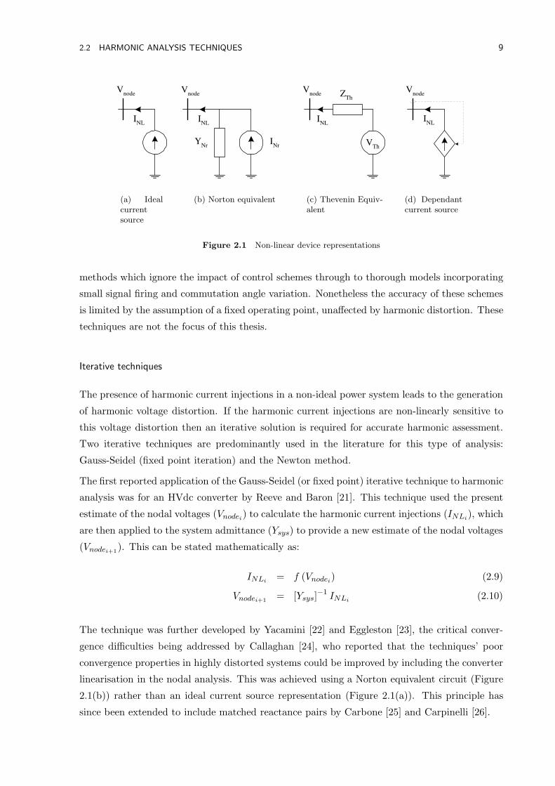
This technique represents the converter as a fixed harmonic current source (Figure 2.1(a)),
ignoring both operating point and terminal voltage variation. An improvement on this technique
is the incorporation of a linearisation of the converter impedance and harmonic transfers. This
leads to either a Norton or Thevenin representation (Figure 2.1(b) and 2.1(c)). Linearised
models have been proposed for both line commutated and hard switched devices, these models
being either experimentally [14] or analytically derived [15]-[20] and ranging in complexity from
2.2 HARMONIC ANALYSIS TECHNIQUES 9
V node
I NL
(a) Idealcurrentsource
V node
I NL
Y Nr
I Nr
(b) Norton equivalent
V node
I NL
Z Th
V Th
(c) Thevenin Equiv-alent
V node
I NL
(d) Dependantcurrent source
Figure 2.1 Non-linear device representations
methods which ignore the impact of control schemes through to thorough models incorporating
small signal firing and commutation angle variation. Nonetheless the accuracy of these schemes
is limited by the assumption of a fixed operating point, unaffected by harmonic distortion. These
techniques are not the focus of this thesis.
Iterative techniques
The presence of harmonic current injections in a non-ideal power system leads to the generation
of harmonic voltage distortion. If the harmonic current injections are non-linearly sensitive to
this voltage distortion then an iterative solution is required for accurate harmonic assessment.
Two iterative techniques are predominantly used in the literature for this type of analysis:
Gauss-Seidel (fixed point iteration) and the Newton method.
The first reported application of the Gauss-Seidel (or fixed point) iterative technique to harmonic
analysis was for an HVdc converter by Reeve and Baron [21]. This technique used the present
estimate of the nodal voltages (Vnodei) to calculate the harmonic current injections (INLi), which
are then applied to the system admittance (Ysys) to provide a new estimate of the nodal voltages
(Vnodei+1). This can be stated mathematically as:
INLi = f (Vnodei) (2.9)
Vnodei+1= [Ysys]
−1 INLi (2.10)
The technique was further developed by Yacamini [22] and Eggleston [23], the critical conver-
gence difficulties being addressed by Callaghan [24], who reported that the techniques’ poor
convergence properties in highly distorted systems could be improved by including the converter
linearisation in the nodal analysis. This was achieved using a Norton equivalent circuit (Figure
2.1(b)) rather than an ideal current source representation (Figure 2.1(a)). This principle has
since been extended to include matched reactance pairs by Carbone [25] and Carpinelli [26].
10 CHAPTER 2 HARMONIC SOLUTION TECHNIQUES AND THEIR APPLICABILITY TO FACTS DEVICES
Initialize Variables
Fundamental frequency
power-flow
Iterative harmonic
solution
Output Solution
New estimate fund. freq.
converter variables
Harmonic / PF
mismatch
No
Yes
Converged
(a) Sequential
Initialize Variables
Power-flow and harmonic
solution
Output solution
No
Yes
Converged
(b) Simultaneous
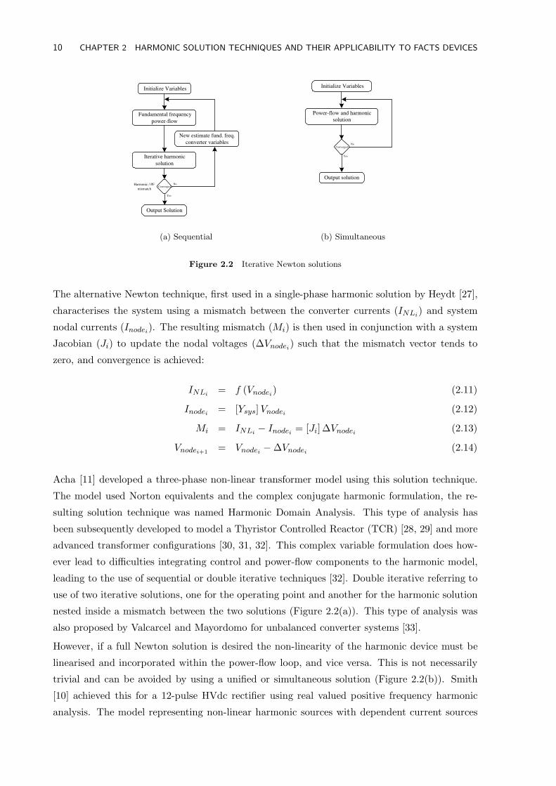
Figure 2.2 Iterative Newton solutions
The alternative Newton technique, first used in a single-phase harmonic solution by Heydt [27],
characterises the system using a mismatch between the converter currents (INLi) and system
nodal currents (Inodei). The resulting mismatch (Mi) is then used in conjunction with a system
Jacobian (Ji) to update the nodal voltages (∆Vnodei) such that the mismatch vector tends to
zero, and convergence is achieved:
INLi = f (Vnodei) (2.11)
Inodei = [Ysys]Vnodei (2.12)
Mi = INLi − Inodei = [Ji]∆Vnodei (2.13)
Vnodei+1= Vnodei − ∆Vnodei (2.14)
Acha [11] developed a three-phase non-linear transformer model using this solution technique.
The model used Norton equivalents and the complex conjugate harmonic formulation, the re-
sulting solution technique was named Harmonic Domain Analysis. This type of analysis has
been subsequently developed to model a Thyristor Controlled Reactor (TCR) [28, 29] and more
advanced transformer configurations [30, 31, 32]. This complex variable formulation does how-
ever lead to difficulties integrating control and power-flow components to the harmonic model,
leading to the use of sequential or double iterative techniques [32]. Double iterative referring to
use of two iterative solutions, one for the operating point and another for the harmonic solution
nested inside a mismatch between the two solutions (Figure 2.2(a)). This type of analysis was
also proposed by Valcarcel and Mayordomo for unbalanced converter systems [33].
However, if a full Newton solution is desired the non-linearity of the harmonic device must be
linearised and incorporated within the power-flow loop, and vice versa. This is not necessarily
trivial and can be avoided by using a unified or simultaneous solution (Figure 2.2(b)). Smith
[10] achieved this for a 12-pulse HVdc rectifier using real valued positive frequency harmonic
analysis. The model representing non-linear harmonic sources with dependent current sources
2.3 APPLICABILITY TO FACTS DEVICES 11
(Figure 2.1(d)), which is mathematically equivalent to using Norton equivalent given a Newton
solution [34]. This simultaneous solution technique was extended by Dinh [35] to unit connected
HVdc rectifiers, and then further by Bathurst [34] who internalised the solution of converter
switching angles, making the model significantly more modular.
2.2.3 Extended harmonic analysis
A recent trend in harmonic research blurs the classical distinction between steady-state and tran-
sient analysis by incorporating time varying ‘dynamic’ harmonic phasors. This principle, first
proposed for resonant power electronic studies by Sanders [36], describes time-domain electrical
quantities using a time variant Fourier series of the form:
x (τ) =
∞∑
k=−∞
Xk (t) ejkωsτ (2.15)
Where Xk(t) are the time evolving Fourier series components calculated by passing a sliding
window (of period T ) over the time domain waveform x (τ). The kth coefficient is calculated
using the ‘averaging’ method:
Xk (t) =1
T
∫ t
t−Tx (τ)e−jkωsτdτ (2.16)
This principle has been extended to multi-phase systems, an example being the Thyristor Con-
trolled Series Capacitor (TCSC) and UPFC models proposed by Stankovic [37]. These models
use the averaging approach to calculate the fundamental frequency Fourier coefficients, which
are then applied to transient analysis. Given the assumption that ac and dc quantities can be
represented by fundamental frequency or dc coefficients respectively it is somewhat questionable
whether this type of analysis is truly harmonic. However Rico [38] has used the same principle
in conjunction with PWM switching functions to represent a STATCOM in isolation excluding
operating point variation. The resultant state space, coined the extended harmonic domain or
the harmonic state space, being capable of both transient and steady-state analysis. Given the
aim of investigating steady-state device interaction, this type of analysis is not the focus of this
thesis.
2.3 APPLICABILITY TO FACTS DEVICES
While harmonic analysis techniques have matured significantly, there still exists a major bias
toward line commutated converters, and relatively small simplified test systems. The distributed
nature of FACTS devices and the move towards higher switching frequencies challenges this bias.
This thesis extends detailed steady-state harmonic analysis to systems containing multiple PWM
FACTS devices.
12 CHAPTER 2 HARMONIC SOLUTION TECHNIQUES AND THEIR APPLICABILITY TO FACTS DEVICES
I STAT
V STAT
(a) STATCOM
I SSSC
V SSSC
(b) SSSC
I Series
V Series
I Shunt
V Shunt
(c) UPFC
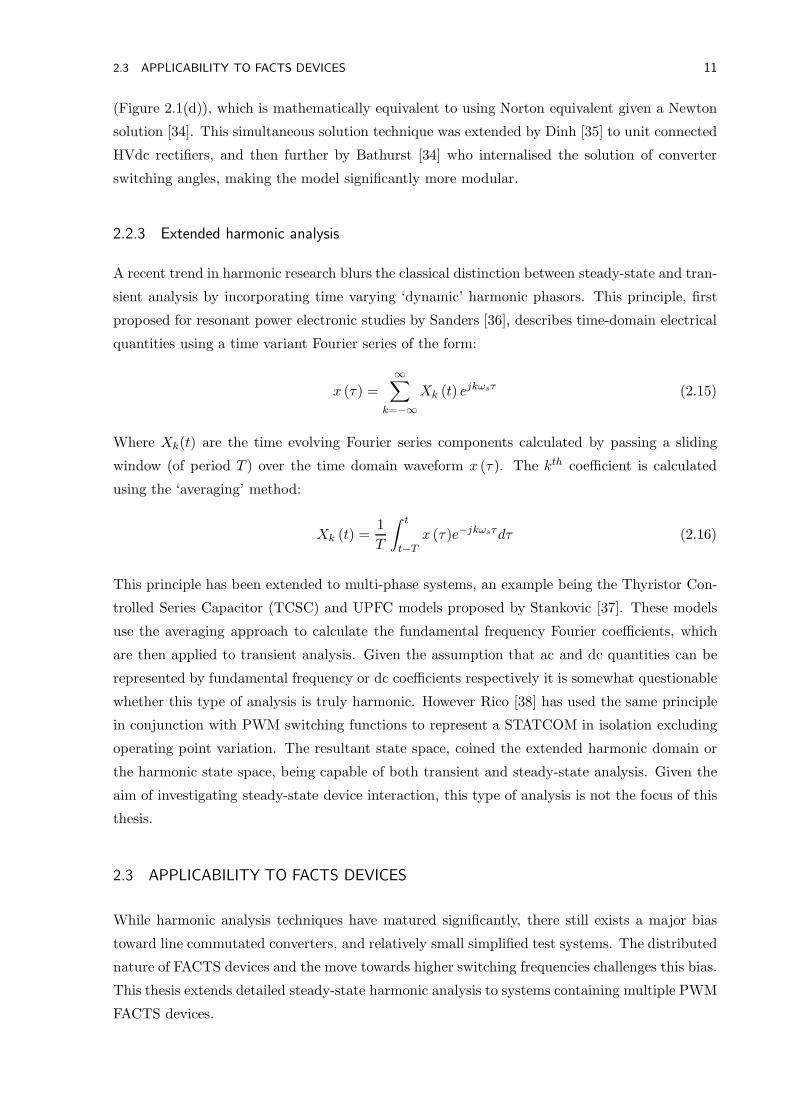
Figure 2.3 VSC FACTS devices under consideration
2.3.1 FACTS devices
The term FACTS, first coined by Hingorani [39, 40, 41], refers to the application of switching
converters to increase the flexibility of traditional power system equipment. This is achieved by
using switching converters as a controllable interface between two power system terminals. A
variety of combinations using this principle exist, providing a wide range of compensation and
control possibilities. Early devices were based on line commutated switching topologies (Static
Var Compensator (SVC) and TCSC) providing limited control flexibility, more advanced sys-
tems (STATCOM, SSSC, Dynamic Voltage Regulator (DVR), UPFC and Interline Power Flow
Controller (IPFC)) being based on the turn off capability of modern semiconductor switches,
which provides enhanced control capabilities.
The analysis described in this thesis is focused on FACTS devices containing hard-switched
PWM bridges, the resulting converter representation being applicable to a variety of connec-
tion configurations. These are typically voltage sourced converters using some form of dc volt-
age source (typically a capacitor) to provide a variable ac voltage source which is capable of
both steady-state reactive power compensation and transient real/reactive power compensation.
Three common connection configurations are considered: shunt, series and hybrid. Examples of
these are shown in Figure 2.3.
2.3.2 Harmonic modelling of FACTS devices
A large variety of analysis techniques have been proposed to analyze FACTS devices. The vast
majority of these models concentrate on transient behaviour using time domain techniques [42]-
[49], these have limited applicability to harmonic analysis. Of the harmonic domain models
proposed, the most thorough have been developed for low pulse number converters: Ricos’ New-
ton based TCR model [28], further developed by Lima [29], and Woods’ linearised STATCOM
[50] are good examples.
While harmonic domain models for PWM FACTS devices do exist they are focused on taking
advantage of the entirely linear harmonic transfer characteristic of hard switched converters.
2.3 APPLICABILITY TO FACTS DEVICES 13
Madrigal [19] for example assumes a fixed operating point (specified separately in a power-
flow) and then uses a linearised Thevenin equivalent to model a single level PWM STATCOM.
Likewise, for the unbalanced PWM model proposed by Saniter [20] which has subsequently been
developed to include linearised firing instant variation [51], yet still depends on an externally
specified operating point. In essence existing work has concentrated on the near linear aspects
of PWM behaviour, rather than the operating point which is the most significant source of
non-linearity.
In contrast iterative techniques can incorporate operating point variation and the interaction
between the harmonic and fundamental frequency solutions, maintaining generality. The cost
being a loss in computational efficiency, the magnitude of which is minimised if the Jacobian is
not recalculated.
2.3.3 Model specification
This thesis details a novel extension to the iterative harmonic solution framework proposed
by Smith [10]; first for individual shunt/series FACTS devices and then to multiple converter
systems. The aim is a comprehensive steady-state analysis technique for FACTS devices, the
associated controllers and system components. To achieve this a generalised formulation capable
of considering the likely harmonic generation mechanisms is proposed, as detailed below:
1. Iterative: A non-linear representation avoids unnecessary assumptions regarding the op-
erating point, making the model capable of analyzing heavily distorted systems where the
harmonic and fundamental frequency solutions are not isolated.
2. Three-phase: Since system unbalance is the primary cause of non-characteristic harmonic
distortion a three-phase formulation is critical.
3. Robust and efficient: A unified Newton is specified in order to provide reliable and efficient
convergence, a requirement for realistically sized test systems.
4. Modular: By maintaining a modular structure for the PWM converter, the model will be
capable of being reconfigured for a range of FACTS devices:
(a) Shunt: STATCOM
(b) Series: SSSC, DVR
(c) Hybrid: UPFC, IPFC
5. Scalable: In order to understand the impact of having multiple FACTS devices interacting
with each other the model must be scalable to larger more complex systems.
6. Control aspects: Harmonic generation is heavily dependent on the operating point of the
converter, as such the model should consider both the operating point, and the impact
harmonics have on this operating point.
14 CHAPTER 2 HARMONIC SOLUTION TECHNIQUES AND THEIR APPLICABILITY TO FACTS DEVICES
Converter 1
Converter i
AC
System
V dc
+
-
R dc
C
I dc 1
I dc i
I dc Cap
DC
System
V dc
V ac
I ac
I dc
I dcCap
Mis
Up
date
Figure 2.4 A diagrammatic overview of the proposed iterative solution technique
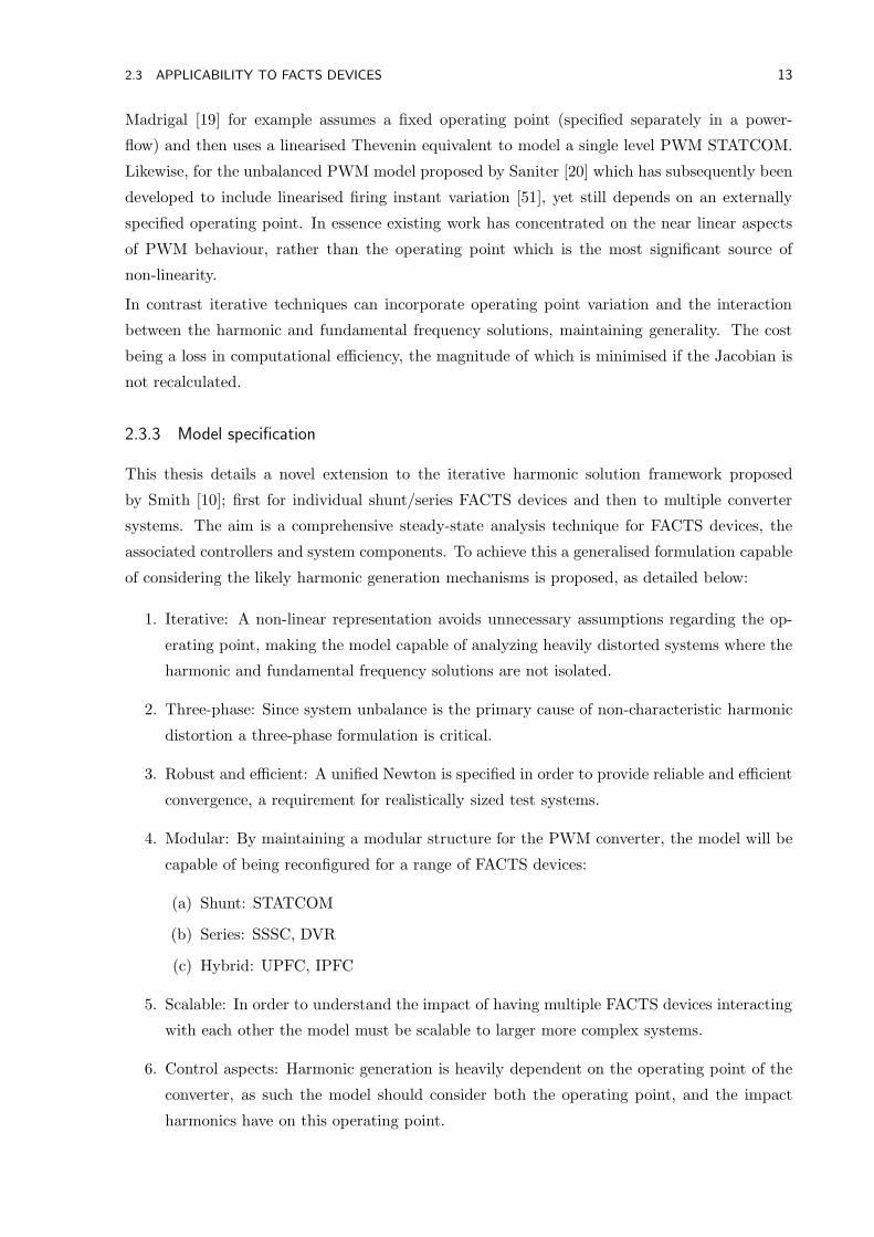
7. Realistic test systems: For full analysis of FACTS devices it is necessary to realistically
model the remainder of the system. Therefore the formulation should be capable of includ-
ing models of relevant system components, any phase coupling and non-linear frequency
dependence.
2.3.4 Model summary
This specification is satisfied by the iterative solution outlined in Figure 2.4. Given the hard
switched nature of PWM devices each converter can be characterised (at harmonic frequencies)
using a single terminal quantity, in this case the dc voltage harmonics. This quantity is initially
estimated and then iteratively updated via a dc current mismatch until convergence is achieved.
The component models and the associated mismatches are described in two steps; first Chapter
3 develops the appropriate harmonic domain models, before Chapter 4 focuses on the application
of these models to a Newton solution. The resultant technique uses convolution (⊗ in Figure
2.4) to describe the ac ↔ dc harmonic transfers for each converter. These transfers form the
basis of the dc current mismatch, which concisely characterises PWM FACTS devices in the
harmonic domain.
Chapter 3
FACTS DEVICE MODELLING IN THE HARMONIC DOMAIN
3.1 INTRODUCTION
The control capabilities which FACTS devices possess are primarily derived from the switching
converters they are based on. This controllable interface, in addition to providing fundamental
frequency and transient control, acts as both a source and modulator of harmonic distortion.
The PWM converter and the associated control block are therefore the central component of any
FACTS device harmonic representation. Since these blocks couple harmonic frequencies they are
naturally non-linear in the time domain. However the extent of this non-linearity is significantly
reduced in the harmonic (or frequency) domain [10], making harmonic domain analysis a concise
solution format.
Chapter 3 outlines how FACTS devices can be represented in the harmonic domain, describing
the hard switched converter transfers (Section 3.2), the connection configuration (Section 3.3)
and the associated control scheme (Section 3.4). These components define an isolated FACTS
device at harmonic frequencies. Finally, in order to permit the generalised harmonic domain
modelling of systems containing multiple FACTS devices, these representations are combined
with a linear network equivalent (Section 3.5).
These harmonic domain models form the basis of non-linear solution proposed in Chapter 4.
The proposed formulation integrates the near linear PWM harmonic transfers with a power-flow
model describing the operating point. To achieve this the PWM transfer model proposed in this
Chapter is reformulated into fundamental and harmonic frequency mismatches, which are then
solved using an iterative Newton solution.
3.1.1 Underlying assumptions and definitions
In order to derive the harmonic domain PWM model the following assumptions / definitions
have been made:
Phase angle reference: Given the complex nature of the electrical quantities represented it
is necessary to define an arbitrary phase reference. This reference would typically be derived
from an ac terminal quantity (using a phase locked loop, PLL); however given the assumption
16 CHAPTER 3 FACTS DEVICE MODELLING IN THE HARMONIC DOMAIN
of a perfect PLL this reference can be placed anywhere within the system. The slack generator
busbar has therefore been defined as the zero angle reference, all firing angles being described
relative to this reference point. This does not preclude full analysis of the PLL, whose error
could be linearised or incorporated as an additional term in the switching instant solution.
Harmonic phasors: Complex valued positive frequency harmonic phasors have been used to
define sinusoidally varying quantities within this thesis. The time domain equivalent of these
phasors, which rotate in an anti-clockwise direction, are defined as the sine referenced imaginary
component.
Network linearity: The harmonic performance of any converter based device is heavily de-
pendant on the ac system to which it is connected, as such the ac network must be represented.
However, fully modelling the entire ac network in a non-linear fashion at harmonic frequencies
would result in a massive increase in the number of solution variables. In order to maintain an
efficient formulation it is advantageous to assume that the ac network behaves in a linear time
invariant fashion (at harmonic frequencies), greatly reducing the number of solution variables.
This assumption limits coupling between harmonic frequencies to components specified by the
mismatch equations.
Idealised switching: The semiconductor switching devices used in the converter bridges are
assumed to perform in an ideal fashion, having zero ON state and an infinite OFF state resis-
tance. This simplifies the switching function derivation, while still permitting switching losses
to be represented as a component of the series connection impedance.
Per unit system: All power system quantities have been incorporated on a per unit (pu) basis,
decreasing the chance of matrix conditioning problems and reducing the internal complexity of
the formulation.
3.2 A PWM CONVERTER MODEL
The primary component of any FACTS device is the switching bridge and a wide variety of con-
verter configurations have been proposed to carry out the controllable interface function. These
configurations range from simplistic single level line commutated configurations (6, 12 pulse etc.),
through single level hard switched PWM, to advanced multi-level multi-switch configurations.
Assuming the devices are hard switched (self-commutated), any arbitrary configuration can
be approximated within the harmonic domain using an ac ↔ dc transfer function which is
predominantly a function of the control variables. As such a generic formulation is proposed,
this permits a range of converter configurations to be incorporated via the transfer function.
For illustrative purposes only the stereotypical six switch three-phase PWM bridge is considered
within this thesis (Figure 3.1).
3.2 A PWM CONVERTER MODEL 17
C R dc
1:1 1
2
5
4
3
6
V a
V b
V c
V Conv
I dc
V dc
+
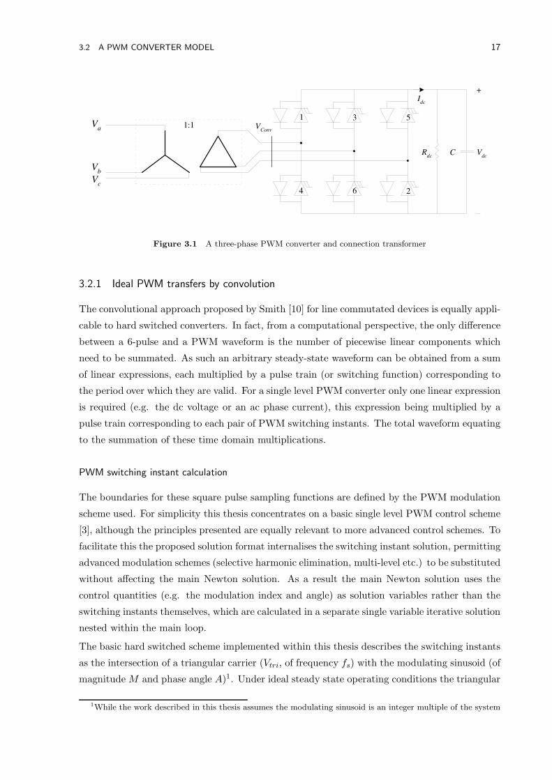
Figure 3.1 A three-phase PWM converter and connection transformer
3.2.1 Ideal PWM transfers by convolution
The convolutional approach proposed by Smith [10] for line commutated devices is equally appli-
cable to hard switched converters. In fact, from a computational perspective, the only difference
between a 6-pulse and a PWM waveform is the number of piecewise linear components which
need to be summated. As such an arbitrary steady-state waveform can be obtained from a sum
of linear expressions, each multiplied by a pulse train (or switching function) corresponding to
the period over which they are valid. For a single level PWM converter only one linear expression
is required (e.g. the dc voltage or an ac phase current), this expression being multiplied by a
pulse train corresponding to each pair of PWM switching instants. The total waveform equating
to the summation of these time domain multiplications.
PWM switching instant calculation
The boundaries for these square pulse sampling functions are defined by the PWM modulation
scheme used. For simplicity this thesis concentrates on a basic single level PWM control scheme
[3], although the principles presented are equally relevant to more advanced control schemes. To
facilitate this the proposed solution format internalises the switching instant solution, permitting
advanced modulation schemes (selective harmonic elimination, multi-level etc.) to be substituted
without affecting the main Newton solution. As a result the main Newton solution uses the
control quantities (e.g. the modulation index and angle) as solution variables rather than the
switching instants themselves, which are calculated in a separate single variable iterative solution
nested within the main loop.
The basic hard switched scheme implemented within this thesis describes the switching instants
as the intersection of a triangular carrier (Vtri, of frequency fs) with the modulating sinusoid (of
magnitude M and phase angle A)1. Under ideal steady state operating conditions the triangular
1While the work described in this thesis assumes the modulating sinusoid is an integer multiple of the system
18 CHAPTER 3 FACTS DEVICE MODELLING IN THE HARMONIC DOMAIN
0 0.5 1 1.50
0.2
0.4
0.6
0.8
1
Angle (radians)
Con
trol
Sig
nals
Triangular Carrier
Distorted Sinusoid
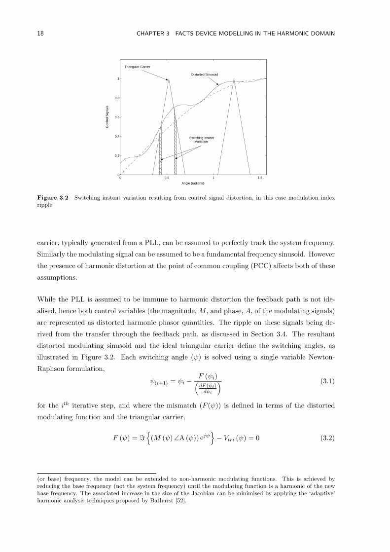
Switching Instant Variation
Figure 3.2 Switching instant variation resulting from control signal distortion, in this case modulation indexripple
carrier, typically generated from a PLL, can be assumed to perfectly track the system frequency.
Similarly the modulating signal can be assumed to be a fundamental frequency sinusoid. However
the presence of harmonic distortion at the point of common coupling (PCC) affects both of these
assumptions.
While the PLL is assumed to be immune to harmonic distortion the feedback path is not ide-
alised, hence both control variables (the magnitude, M , and phase, A, of the modulating signals)
are represented as distorted harmonic phasor quantities. The ripple on these signals being de-
rived from the transfer through the feedback path, as discussed in Section 3.4. The resultant
distorted modulating sinusoid and the ideal triangular carrier define the switching angles, as
illustrated in Figure 3.2. Each switching angle (ψ) is solved using a single variable Newton-
Raphson formulation,
ψ(i+1) = ψi −F (ψi)
(dF (ψi)dψi
) (3.1)
for the ith iterative step, and where the mismatch (F (ψ)) is defined in terms of the distorted
modulating function and the triangular carrier,
F (ψ) = ℑ
(M (ψ) ∠A(ψ)) ejψ
− Vtri (ψ) = 0 (3.2)
(or base) frequency, the model can be extended to non-harmonic modulating functions. This is achieved byreducing the base frequency (not the system frequency) until the modulating function is a harmonic of the newbase frequency. The associated increase in the size of the Jacobian can be minimised by applying the ‘adaptive’harmonic analysis techniques proposed by Bathurst [52].
3.2 A PWM CONVERTER MODEL 19
1
-1
2π
δψ
δm
Vtri
↑ m
ψ1 ψ2
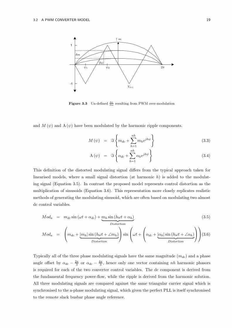
Figure 3.3 Un-defined δψ
δmresulting from PWM over-modulation
and M (ψ) and A (ψ) have been modulated by the harmonic ripple components.
M (ψ) = ℑ
mdc +nh∑
h=1
mhejhψ
(3.3)
A (ψ) = ℑ
αdc +
nh∑
h=1
αhejhψ
(3.4)
This definition of the distorted modulating signal differs from the typical approach taken for
linearised models, where a small signal distortion (at harmonic h) is added to the modulat-
ing signal (Equation 3.5). In contrast the proposed model represents control distortion as the
multiplication of sinusoids (Equation 3.6). This representation more closely replicates realistic
methods of generating the modulating sinusoid, which are often based on modulating two almost
dc control variables.
Moda = mdc sin (ωt+ αdc) +mh sin (hωt + αh)︸ ︷︷ ︸
Distortion
(3.5)
Moda =
mdc + |mh| sin (hωt+ ∠mh)︸ ︷︷ ︸
Distortion
sin
ωt+
αdc + |αh| sin (hωt+ ∠αh)︸ ︷︷ ︸
Distortion
(3.6)
Typically all of the three phase modulating signals have the same magnitude (mdc) and a phase
angle offset by αdc −2π3 or αdc −
4π3 , hence only one vector containing nh harmonic phasors
is required for each of the two converter control variables. The dc component is derived from
the fundamental frequency power-flow, while the ripple is derived from the harmonic solution.
All three modulating signals are compared against the same triangular carrier signal which is
synchronised to the a-phase modulating signal, which given the perfect PLL is itself synchronised
to the remote slack busbar phase angle reference.
20 CHAPTER 3 FACTS DEVICE MODELLING IN THE HARMONIC DOMAIN
ψON1ψOF F1
ψON2ψOF F2
2π
1
Np
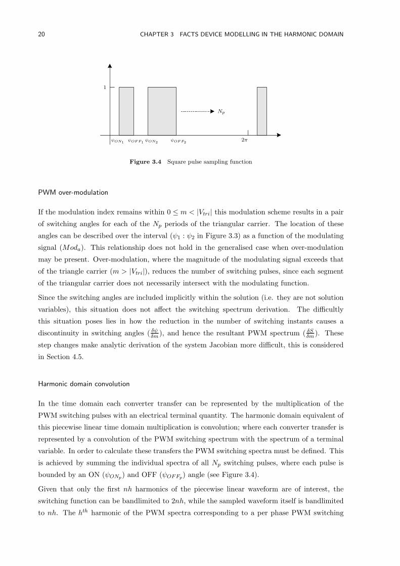
Figure 3.4 Square pulse sampling function
PWM over-modulation
If the modulation index remains within 0 ≤ m < |Vtri| this modulation scheme results in a pair
of switching angles for each of the Np periods of the triangular carrier. The location of these
angles can be described over the interval (ψ1 : ψ2 in Figure 3.3) as a function of the modulating
signal (Moda). This relationship does not hold in the generalised case when over-modulation
may be present. Over-modulation, where the magnitude of the modulating signal exceeds that
of the triangle carrier (m > |Vtri|), reduces the number of switching pulses, since each segment
of the triangular carrier does not necessarily intersect with the modulating function.
Since the switching angles are included implicitly within the solution (i.e. they are not solution
variables), this situation does not affect the switching spectrum derivation. The difficultly
this situation poses lies in how the reduction in the number of switching instants causes a
discontinuity in switching angles ( δψδm), and hence the resultant PWM spectrum ( δSδm). These
step changes make analytic derivation of the system Jacobian more difficult, this is considered
in Section 4.5.
Harmonic domain convolution
In the time domain each converter transfer can be represented by the multiplication of the
PWM switching pulses with an electrical terminal quantity. The harmonic domain equivalent of
this piecewise linear time domain multiplication is convolution; where each converter transfer is
represented by a convolution of the PWM switching spectrum with the spectrum of a terminal
variable. In order to calculate these transfers the PWM switching spectra must be defined. This
is achieved by summing the individual spectra of all Np switching pulses, where each pulse is
bounded by an ON (ψONp) and OFF (ψOFFp) angle (see Figure 3.4).
Given that only the first nh harmonics of the piecewise linear waveform are of interest, the
switching function can be bandlimited to 2nh, while the sampled waveform itself is bandlimited
to nh. The hth harmonic of the PWM spectra corresponding to a per phase PWM switching
3.2 A PWM CONVERTER MODEL 21
function can therefore be described using Fourier analysis,
Sh =
Np∑
p=1
j
2π
(ψOFFp − ψONp
), h = 0 (3.7)
Sh =
Np∑
p=1
(
ejhψOFFp − ejhψONp)∗
hπ, h 6= 0 (3.8)
where the OFF (ψOFFp) angle must occur after the associated ON (ψONp) angle.
The convolution itself is defined using the conjugate operator (replacing the requirement for neg-
ative frequency harmonics), leading to the following definition which describes the convolution
of a PWM switching spectrum (S) with a generic bandlimited signal (F ) [53]. The kth harmonic
of the resulting spectra being:
(F ⊗ S)k =j
2
−2F0S0 +
nh∑
q=0
FqS∗q
, k = 0 (3.9)
(F ⊗ S)k =j
2
nh∑
q=0
(
FqS∗(q+k)
)∗
−
k∑
q=0
FqS∗(k−q) +
nh∑
q=k
FqS∗(q−k)
, k > 0 (3.10)
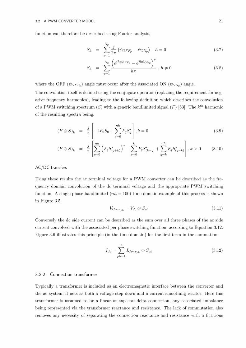
AC/DC transfers
Using these results the ac terminal voltage for a PWM converter can be described as the fre-
quency domain convolution of the dc terminal voltage and the appropriate PWM switching
function. A single-phase bandlimited (nh = 100) time domain example of this process is shown
in Figure 3.5.
VConvph = Vdc ⊗ Sph (3.11)
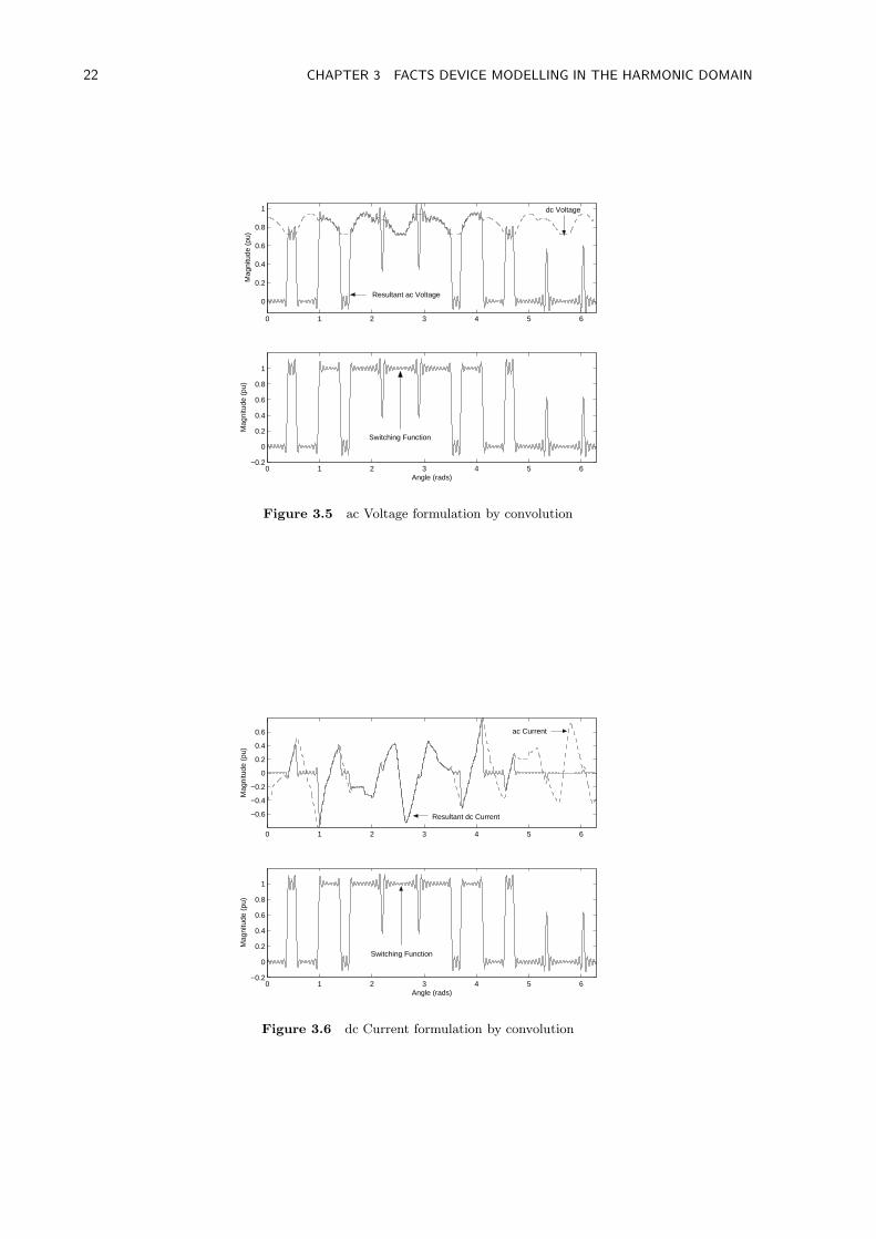
Conversely the dc side current can be described as the sum over all three phases of the ac side
current convolved with the associated per phase switching function, according to Equation 3.12.
Figure 3.6 illustrates this principle (in the time domain) for the first term in the summation.
Idc =3∑
ph=1
IConvph ⊗ Sph (3.12)
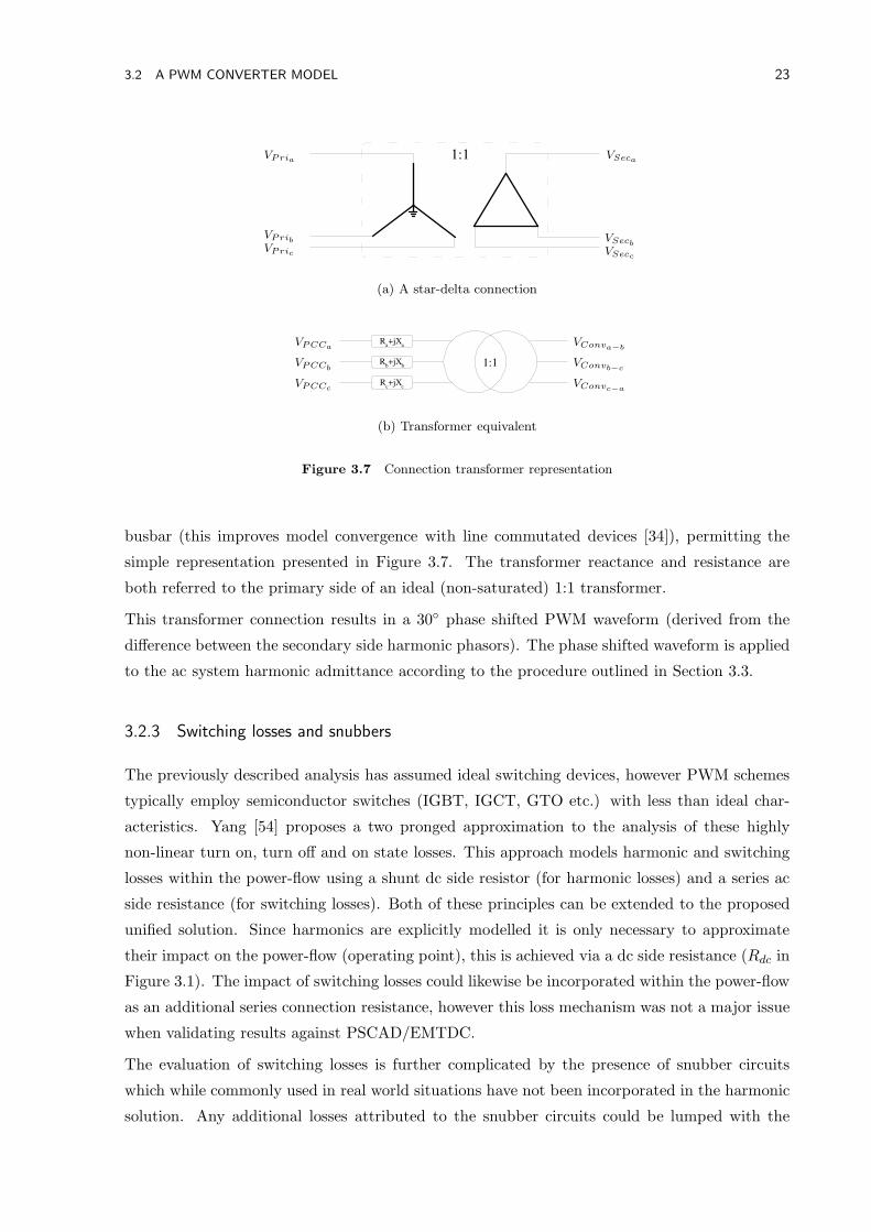
3.2.2 Connection transformer
Typically a transformer is included as an electromagnetic interface between the converter and
the ac system; it acts as both a voltage step down and a current smoothing reactor. Here this
transformer is assumed to be a linear on-tap star-delta connection, any associated imbalance
being represented via the transformer reactance and resistance. The lack of commutation also
removes any necessity of separating the connection reactance and resistance with a fictitious
22 CHAPTER 3 FACTS DEVICE MODELLING IN THE HARMONIC DOMAIN
0 1 2 3 4 5 6
0
0.2
0.4
0.6
0.8
1
Mag
nitu
de (
pu)
0 1 2 3 4 5 6−0.2
0
0.2
0.4
0.6
0.8
1
Angle (rads)
Mag
nitu
de (
pu)
Switching Function
dc Voltage
Resultant ac Voltage
Figure 3.5 ac Voltage formulation by convolution
0 1 2 3 4 5 6
−0.6
−0.4
−0.2
0
0.2
0.4
0.6
Mag
nitu
de (
pu)
0 1 2 3 4 5 6−0.2
0
0.2
0.4
0.6
0.8
1
Angle (rads)
Mag
nitu
de (
pu)
Switching Function
ac Current
Resultant dc Current
Figure 3.6 dc Current formulation by convolution
3.2 A PWM CONVERTER MODEL 23
1:1 VPria
VPribVPric
VSeca
VSecb
VSecc
(a) A star-delta connection
1:1
R a +jX
a
R b +jX
b
R c +jX
c
VPCCa
VPCCb
VPCCc
VConva−b
VConvb−c
VConvc−a
(b) Transformer equivalent
Figure 3.7 Connection transformer representation
busbar (this improves model convergence with line commutated devices [34]), permitting the
simple representation presented in Figure 3.7. The transformer reactance and resistance are
both referred to the primary side of an ideal (non-saturated) 1:1 transformer.
This transformer connection results in a 30 phase shifted PWM waveform (derived from the
difference between the secondary side harmonic phasors). The phase shifted waveform is applied
to the ac system harmonic admittance according to the procedure outlined in Section 3.3.
3.2.3 Switching losses and snubbers
The previously described analysis has assumed ideal switching devices, however PWM schemes
typically employ semiconductor switches (IGBT, IGCT, GTO etc.) with less than ideal char-
acteristics. Yang [54] proposes a two pronged approximation to the analysis of these highly
non-linear turn on, turn off and on state losses. This approach models harmonic and switching
losses within the power-flow using a shunt dc side resistor (for harmonic losses) and a series ac
side resistance (for switching losses). Both of these principles can be extended to the proposed
unified solution. Since harmonics are explicitly modelled it is only necessary to approximate
their impact on the power-flow (operating point), this is achieved via a dc side resistance (Rdc in
Figure 3.1). The impact of switching losses could likewise be incorporated within the power-flow
as an additional series connection resistance, however this loss mechanism was not a major issue
when validating results against PSCAD/EMTDC.
The evaluation of switching losses is further complicated by the presence of snubber circuits
which while commonly used in real world situations have not been incorporated in the harmonic
solution. Any additional losses attributed to the snubber circuits could be lumped with the
24 CHAPTER 3 FACTS DEVICE MODELLING IN THE HARMONIC DOMAIN
V Conv
V i
I shunt
Z shunt
(a) Shunt connection
V Conv
V i
I shunt
Z shunt
h
h
h
(b) Harmonic equivalent at har-monic h
Figure 3.8 Shunt connection representation (single line diagram)
switching losses; the accurate assessment of these losses would require additional analysis not
included within this thesis.
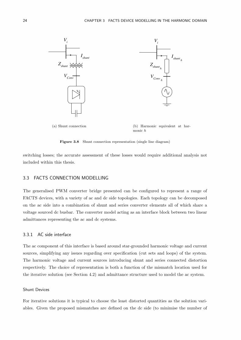
3.3 FACTS CONNECTION MODELLING
The generalised PWM converter bridge presented can be configured to represent a range of
FACTS devices, with a variety of ac and dc side topologies. Each topology can be decomposed
on the ac side into a combination of shunt and series converter elements all of which share a
voltage sourced dc busbar. The converter model acting as an interface block between two linear
admittances representing the ac and dc systems.
3.3.1 AC side interface
The ac component of this interface is based around star-grounded harmonic voltage and current
sources, simplifying any issues regarding over specification (cut sets and loops) of the system.
The harmonic voltage and current sources introducing shunt and series connected distortion
respectively. The choice of representation is both a function of the mismatch location used for
the iterative solution (see Section 4.2) and admittance structure used to model the ac system.
Shunt Devices
For iterative solutions it is typical to choose the least distorted quantities as the solution vari-
ables. Given the proposed mismatches are defined on the dc side (to minimise the number of
3.3 FACTS CONNECTION MODELLING 25
V Conv
V i
I series
Z series
V j
(a) Series connection
V i Z
series V
j
I series
I series
h h
h
(b) Harmonic equivalent at harmonich
Figure 3.9 Series connection representation (single line diagram)
solution variables) and voltage sourced conversion is assumed, the best choice of variable is the
dc voltage. This choice makes it convenient to represent the ac side of a shunt connected con-
verter using voltage sources; primarily since the only processing required to generate the phase
voltages is the PWM dc ↔ ac transfer. In contrast a shunt current injection representation
[55] would require an additional conversion step or a different choice of variables, both of which
would affect computational efficiency.
The voltage source representation is also very easy to incorporate within linear harmonic analysis,
all that is required is an additional voltage defined busbar connected through the transformer
impedance to the PCC (see Figure 3.8). The voltage on the new busbar being equal to the
converters ac terminal voltage (e.g. VConva−b = VConva − VConvb), as defined in Section 3.2.
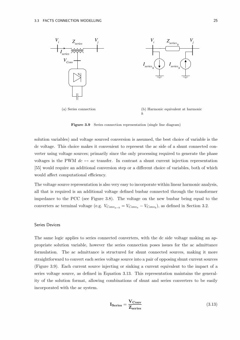
Series Devices
The same logic applies to series connected converters, with the dc side voltage making an ap-
propriate solution variable, however the series connection poses issues for the ac admittance
formulation. The ac admittance is structured for shunt connected sources, making it more
straightforward to convert each series voltage source into a pair of opposing shunt current sources
(Figure 3.9). Each current source injecting or sinking a current equivalent to the impact of a
series voltage source, as defined in Equation 3.13. This representation maintains the general-
ity of the solution format, allowing combinations of shunt and series converters to be easily
incorporated with the ac system.
ISeries =VConv
Zseries
(3.13)
26 CHAPTER 3 FACTS DEVICE MODELLING IN THE HARMONIC DOMAIN
V shunt
V i
Z shunt
Z series
V j
I series
I series h
h
h h
h
Figure 3.10 A harmonic voltage/current source UPFC model (single line diagram)
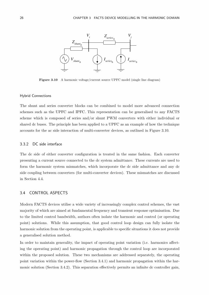
Hybrid Connections
The shunt and series converter blocks can be combined to model more advanced connection
schemes such as the UPFC and IPFC. This representation can be generalised to any FACTS
scheme which is composed of series and/or shunt PWM converters with either individual or
shared dc buses. The principle has been applied to a UPFC as an example of how the technique
accounts for the ac side interaction of multi-converter devices, as outlined in Figure 3.10.
3.3.2 DC side interface
The dc side of either converter configuration is treated in the same fashion. Each converter
presenting a current source connected to the dc system admittance. These currents are used to
form the harmonic system mismatches, which incorporate the dc side admittance and any dc
side coupling between converters (for multi-converter devices). These mismatches are discussed
in Section 4.4.
3.4 CONTROL ASPECTS
Modern FACTS devices utilise a wide variety of increasingly complex control schemes, the vast
majority of which are aimed at fundamental frequency and transient response optimisation. Due
to the limited control bandwidth, authors often isolate the harmonic and control (or operating
point) solutions. While this assumption, that good control loop design can fully isolate the
harmonic solution from the operating point, is applicable to specific situations it does not provide
a generalised solution method.
In order to maintain generality, the impact of operating point variation (i.e. harmonics affect-
ing the operating point) and harmonic propagation through the control loop are incorporated
within the proposed solution. These two mechanisms are addressed separately, the operating
point variation within the power-flow (Section 3.4.1) and harmonic propagation within the har-
monic solution (Section 3.4.2). This separation effectively permits an infinite dc controller gain,
3.4 CONTROL ASPECTS 27
resulting in the correct operating point, without the associated numerical difficulties of incorpo-
rating zero frequency control components within the harmonic matrices (the PI controller has a
pole at zero frequency).
While a massive variety of control techniques could be modelled (to differing extents) in HDA,
this thesis focuses on common (and basic) voltage, current and power regulation schemes which
are not necessarily optimised for transient response. These control schemes are succinctly in-
cluded using a combination of two control blocks; one based on fundamental frequency real/reactive
power flows and the other a single variable PI control loop.
3.4.1 Fundamental frequency component
Since most FACTS controllers are principally aimed at regulating fundamental frequency quanti-
ties, the most significant control aspect is the component associated with fundamental frequency.
This component is dealt with in the power-flow section of the model using classic mismatches
between a set-point and the current value. These mismatches can be used in isolation, given the
assumption of ‘pseudo fundamental’ control quantities, or as the dc component of a distorted
control mismatch. The first option improves efficiency when modelling large systems with mul-
tiple FACTS devices, the second being more appropriate for detailed analysis of a single device.
Real and reactive power control schemes
The assumption that the harmonics do not propagate through the controller is particularly
applicable to control schemes which regulate real or reactive power since these quantities are
predominantly a function of fundamental frequency quantities. The limited bandwidth of me-
tering transducers and the requirement that both harmonic voltage and current must be present
at the same harmonic to generate real or reactive power, make the assumption of harmonic iso-
lation fair in all but the most distorted systems. Given this assumption fundamental frequency
real/reactive control schemes can be implemented entirely within the power-flow solution block.
For example the series element of a UPFC, controlled to regulate both the positive sequence real
and reactive power being transferred through an adjacent transmission system is represented
using two simple mismatches:
0 = P+Line − POrder (3.14)
0 = Q+Line −QOrder (3.15)
Since single converter FACTS devices are limited to reactive power compensation (in the steady-
state), the associated STATCOM and SSSC reactive power control schemes can be modelled
using a single Q mismatch.
28 CHAPTER 3 FACTS DEVICE MODELLING IN THE HARMONIC DOMAIN
Voltage and current control schemes
While voltage and current quantities are often more distorted than power quantities it is some-
times useful to make the somewhat questionable assumption that these quantities too can be
isolated from the harmonic solution. This is done primarily because incorporating harmonic
propagation through the controller requires significantly more computational effort.
For phase angle control schemes the power-flow mismatches state that the positive sequence
voltage at the PCC (or current through the converter) must equate to the corresponding voltage
(or current) order, while the magnitude of the modulating index (mdc) must equate to the fixed
modulating index order (mOrder). The second modulating index mismatches can be replaced by
a dc voltage mismatch in regulated dc busbar schemes.
For a STATCOM, with an optional droop characteristic (XDroop):
0 = V +PCC − VOrder +XDroopI
+STAT (3.16)
0 = mdc −mOrder (3.17)
For an SSSC:
0 = I+SSSC − IOrder (3.18)
0 = mdc −mOrder (3.19)
3.4.2 Distorted control feedback
If the measurement point is heavily distorted, or the converter controller is aimed at fast tran-
sient response (hence requiring wider control bandwidth), it is necessary to assess the impact
of harmonic propagation through the controller. This can be achieved by incorporating the fre-
quency response of the controller within the harmonic solution. The proposed formulation, while
capable of incorporating any linear (or linearised) controller, is described here with reference to a
basic PI feedback loop (Figure 3.11). While extremely simple this demonstrates how this mech-
anism can impact the fundamental and harmonic frequency solutions. If a non-linear control
scheme were to be included the number and location of the control mismatches (described in
Section 4.4.4) would need to be adjusted.
These control loops are typically used to adjust the phase (α) and/or magnitude (m) of the PWM
modulating function in order to regulate an ac or dc quantity. The basic example given here
regulates an ac quantity using phase angle control, which indirectly adjusts the the magnitude
of the converter’s terminal voltage. This basic principle is applied to more advanced schemes in
later chapters, obviously the dq transformation can be omitted for control schemes based on dc
quantities (e.g. regulated dc busbar systems).
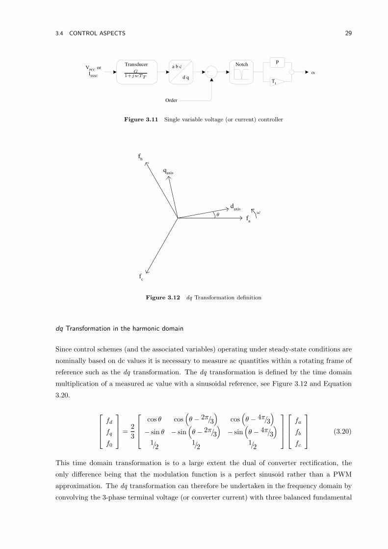
3.4 CONTROL ASPECTS 29
Transducer a b c
d q
P
T I
Notch V
PCC or
I SSSC
Order
G1+jwTT
α
Figure 3.11 Single variable voltage (or current) controller
f a
f b
f c
q axis
d axis
ωθ
Figure 3.12 dq Transformation definition
dq Transformation in the harmonic domain
Since control schemes (and the associated variables) operating under steady-state conditions are
nominally based on dc values it is necessary to measure ac quantities within a rotating frame of
reference such as the dq transformation. The dq transformation is defined by the time domain
multiplication of a measured ac value with a sinusoidal reference, see Figure 3.12 and Equation
3.20.
fd
fq
f0
=2
3
cos θ cos(
θ − 2π/3
)
cos(
θ − 4π/3
)
− sin θ − sin(
θ − 2π/3
)
− sin(
θ − 4π/3
)
1/21/2
1/2
fa
fb
fc
(3.20)
This time domain transformation is to a large extent the dual of converter rectification, the
only difference being that the modulation function is a perfect sinusoid rather than a PWM
approximation. The dq transformation can therefore be undertaken in the frequency domain by
convolving the 3-phase terminal voltage (or converter current) with three balanced fundamental
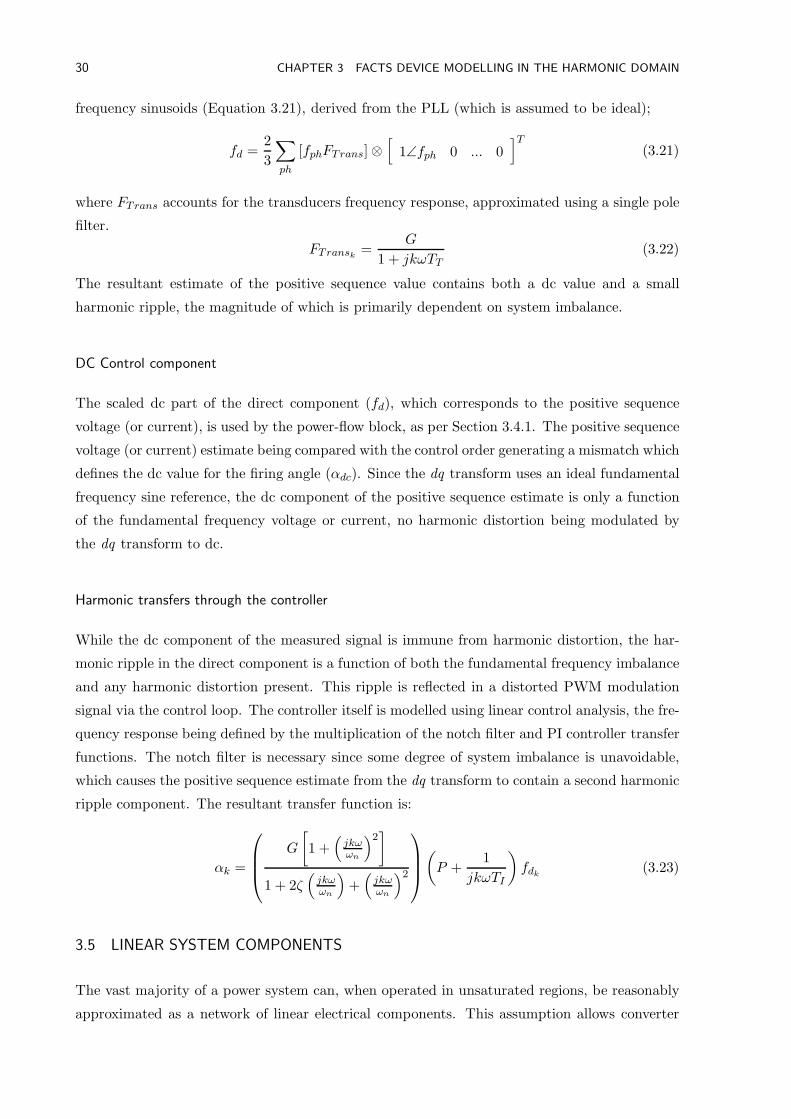
30 CHAPTER 3 FACTS DEVICE MODELLING IN THE HARMONIC DOMAIN
frequency sinusoids (Equation 3.21), derived from the PLL (which is assumed to be ideal);
fd =2
3
∑
ph
[fphFTrans] ⊗[
1∠fph 0 ... 0]T
(3.21)
where FTrans accounts for the transducers frequency response, approximated using a single pole
filter.
FTransk =G
1 + jkωTT(3.22)
The resultant estimate of the positive sequence value contains both a dc value and a small
harmonic ripple, the magnitude of which is primarily dependent on system imbalance.
DC Control component
The scaled dc part of the direct component (fd), which corresponds to the positive sequence
voltage (or current), is used by the power-flow block, as per Section 3.4.1. The positive sequence
voltage (or current) estimate being compared with the control order generating a mismatch which
defines the dc value for the firing angle (αdc). Since the dq transform uses an ideal fundamental
frequency sine reference, the dc component of the positive sequence estimate is only a function
of the fundamental frequency voltage or current, no harmonic distortion being modulated by
the dq transform to dc.
Harmonic transfers through the controller
While the dc component of the measured signal is immune from harmonic distortion, the har-
monic ripple in the direct component is a function of both the fundamental frequency imbalance
and any harmonic distortion present. This ripple is reflected in a distorted PWM modulation
signal via the control loop. The controller itself is modelled using linear control analysis, the fre-
quency response being defined by the multiplication of the notch filter and PI controller transfer
functions. The notch filter is necessary since some degree of system imbalance is unavoidable,
which causes the positive sequence estimate from the dq transform to contain a second harmonic
ripple component. The resultant transfer function is:
αk =
G
[
1 +(jkωωn
)2]
1 + 2ζ(jkωωn
)
+(jkωωn
)2
(
P +1
jkωTI
)
fdk (3.23)
3.5 LINEAR SYSTEM COMPONENTS
The vast majority of a power system can, when operated in unsaturated regions, be reasonably
approximated as a network of linear electrical components. This assumption allows converter
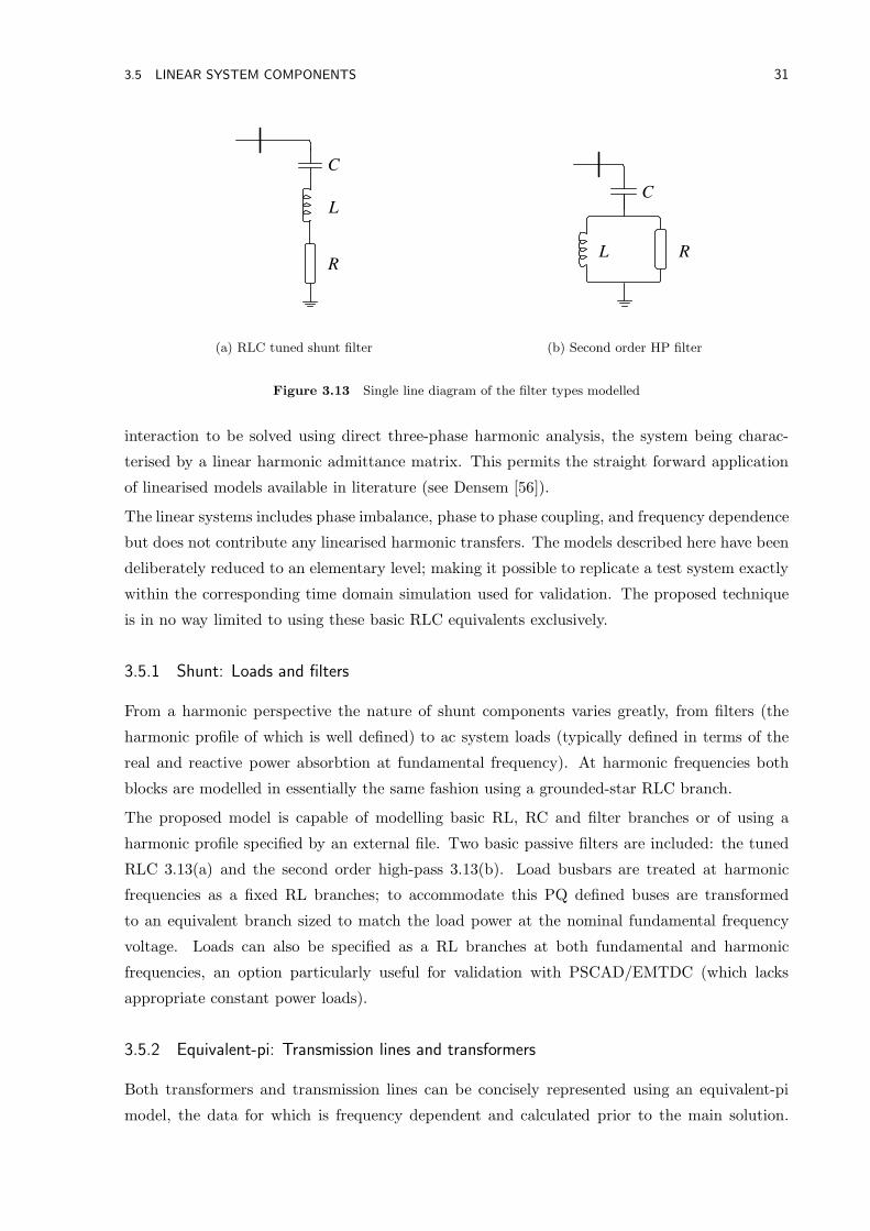
3.5 LINEAR SYSTEM COMPONENTS 31
C
R
L
(a) RLC tuned shunt filter
C
R L
(b) Second order HP filter
Figure 3.13 Single line diagram of the filter types modelled
interaction to be solved using direct three-phase harmonic analysis, the system being charac-
terised by a linear harmonic admittance matrix. This permits the straight forward application
of linearised models available in literature (see Densem [56]).
The linear systems includes phase imbalance, phase to phase coupling, and frequency dependence
but does not contribute any linearised harmonic transfers. The models described here have been
deliberately reduced to an elementary level; making it possible to replicate a test system exactly
within the corresponding time domain simulation used for validation. The proposed technique
is in no way limited to using these basic RLC equivalents exclusively.
3.5.1 Shunt: Loads and filters
From a harmonic perspective the nature of shunt components varies greatly, from filters (the
harmonic profile of which is well defined) to ac system loads (typically defined in terms of the
real and reactive power absorbtion at fundamental frequency). At harmonic frequencies both
blocks are modelled in essentially the same fashion using a grounded-star RLC branch.
The proposed model is capable of modelling basic RL, RC and filter branches or of using a
harmonic profile specified by an external file. Two basic passive filters are included: the tuned
RLC 3.13(a) and the second order high-pass 3.13(b). Load busbars are treated at harmonic
frequencies as a fixed RL branches; to accommodate this PQ defined buses are transformed
to an equivalent branch sized to match the load power at the nominal fundamental frequency
voltage. Loads can also be specified as a RL branches at both fundamental and harmonic
frequencies, an option particularly useful for validation with PSCAD/EMTDC (which lacks
appropriate constant power loads).
3.5.2 Equivalent-pi: Transmission lines and transformers
Both transformers and transmission lines can be concisely represented using an equivalent-pi
model, the data for which is frequency dependent and calculated prior to the main solution.
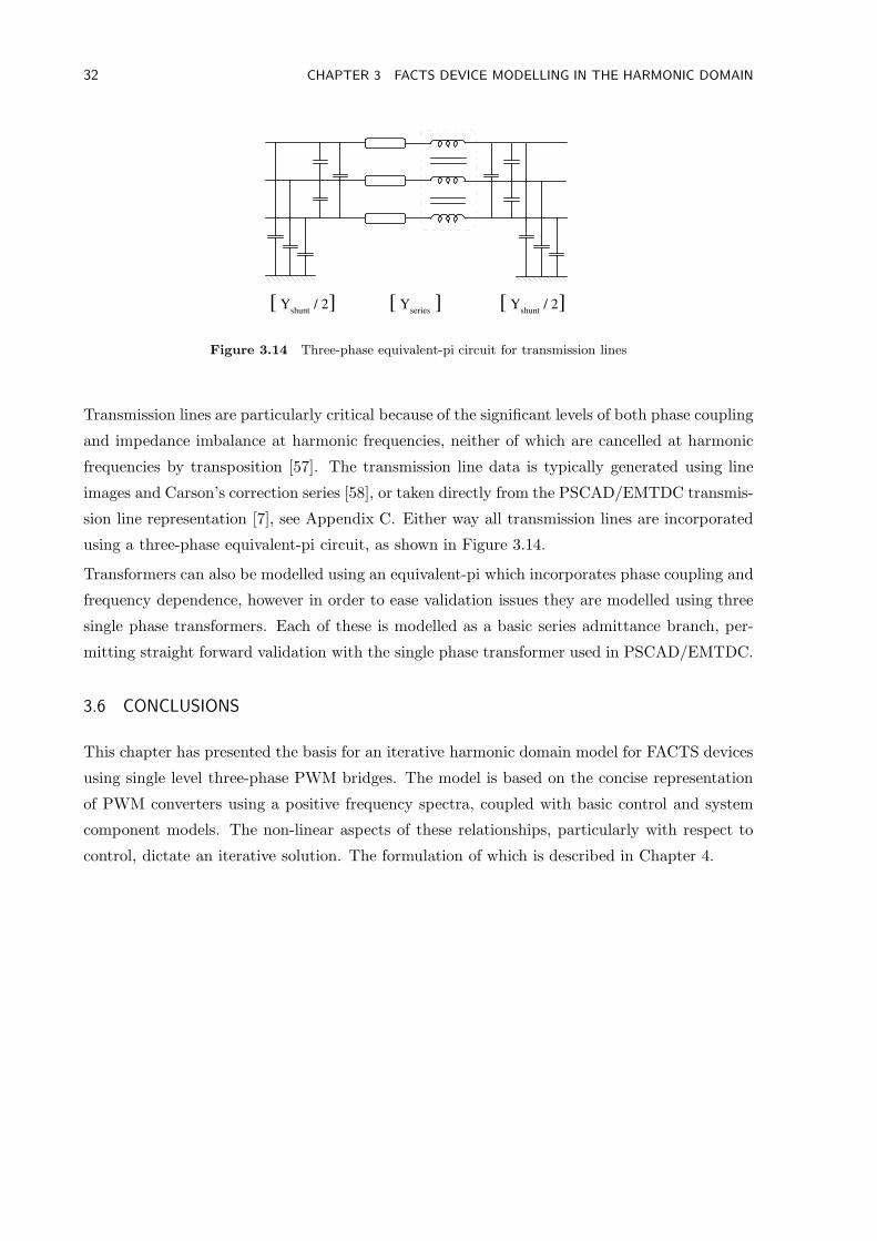
32 CHAPTER 3 FACTS DEVICE MODELLING IN THE HARMONIC DOMAIN
[ Y shunt
/ 2 ] [ Y shunt
/ 2 ] [ Y series
]
Figure 3.14 Three-phase equivalent-pi circuit for transmission lines
Transmission lines are particularly critical because of the significant levels of both phase coupling
and impedance imbalance at harmonic frequencies, neither of which are cancelled at harmonic
frequencies by transposition [57]. The transmission line data is typically generated using line
images and Carson’s correction series [58], or taken directly from the PSCAD/EMTDC transmis-
sion line representation [7], see Appendix C. Either way all transmission lines are incorporated
using a three-phase equivalent-pi circuit, as shown in Figure 3.14.
Transformers can also be modelled using an equivalent-pi which incorporates phase coupling and
frequency dependence, however in order to ease validation issues they are modelled using three
single phase transformers. Each of these is modelled as a basic series admittance branch, per-
mitting straight forward validation with the single phase transformer used in PSCAD/EMTDC.
3.6 CONCLUSIONS
This chapter has presented the basis for an iterative harmonic domain model for FACTS devices
using single level three-phase PWM bridges. The model is based on the concise representation
of PWM converters using a positive frequency spectra, coupled with basic control and system
component models. The non-linear aspects of these relationships, particularly with respect to
control, dictate an iterative solution. The formulation of which is described in Chapter 4.
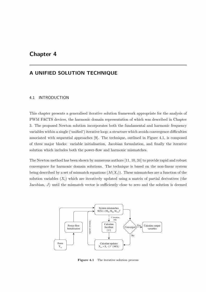
Chapter 4
A UNIFIED SOLUTION TECHNIQUE
4.1 INTRODUCTION
This chapter presents a generalised iterative solution framework appropriate for the analysis of
PWM FACTS devices, the harmonic domain representation of which was described in Chapter
3. The proposed Newton solution incorporates both the fundamental and harmonic frequency
variables within a single (‘unified’) iterative loop; a structure which avoids convergence difficulties
associated with sequential approaches [9]. The technique, outlined in Figure 4.1, is composed
of three major blocks: variable initialisation, Jacobian formulation, and finally the iterative
solution which includes both the power-flow and harmonic mismatches.
The Newton method has been shown by numerous authors [11, 10, 34] to provide rapid and robust
convergence for harmonic domain solutions. The technique is based on the non-linear system
being described by a set of mismatch equations (M(Xi)). These mismatches are a function of the
solution variables (Xi) which are iteratively updated using a matrix of partial derivatives (the
Jacobian, J) until the mismatch vector is sufficiently close to zero and the solution is deemed
No
Yes
System mismatches M(X i ) = [M
PF M
Idc M
Con ] T
Calculate
Jacobian
[ J ]
Converged
Calculate updates X
i+1 = X
i - [ J -1 ] M(X
i )
Calculate output
variables
Power-flow
Initialization
Form
Y ac
Solu
tion
variab
les
1 st iteration
only
Figure 4.1 The iterative solution process
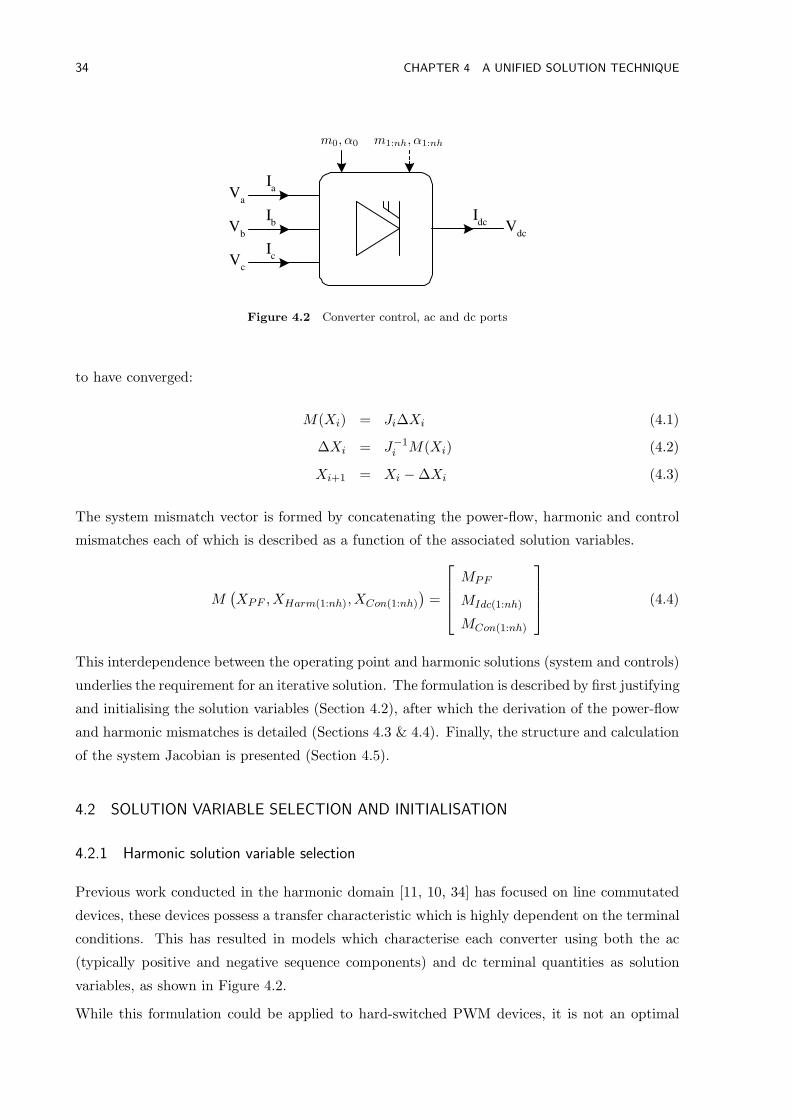
34 CHAPTER 4 A UNIFIED SOLUTION TECHNIQUE
V a
V b
V c
I a
I b
I c
V dc
I dc
m0, α0 m1:nh, α1:nh
Figure 4.2 Converter control, ac and dc ports
to have converged:
M(Xi) = Ji∆Xi (4.1)
∆Xi = J−1i M(Xi) (4.2)
Xi+1 = Xi − ∆Xi (4.3)
The system mismatch vector is formed by concatenating the power-flow, harmonic and control
mismatches each of which is described as a function of the associated solution variables.
M(XPF ,XHarm(1:nh),XCon(1:nh)
)=
MPF
MIdc(1:nh)
MCon(1:nh)
(4.4)
This interdependence between the operating point and harmonic solutions (system and controls)
underlies the requirement for an iterative solution. The formulation is described by first justifying
and initialising the solution variables (Section 4.2), after which the derivation of the power-flow
and harmonic mismatches is detailed (Sections 4.3 & 4.4). Finally, the structure and calculation
of the system Jacobian is presented (Section 4.5).
4.2 SOLUTION VARIABLE SELECTION AND INITIALISATION
4.2.1 Harmonic solution variable selection
Previous work conducted in the harmonic domain [11, 10, 34] has focused on line commutated
devices, these devices possess a transfer characteristic which is highly dependent on the terminal
conditions. This has resulted in models which characterise each converter using both the ac
(typically positive and negative sequence components) and dc terminal quantities as solution
variables, as shown in Figure 4.2.
While this formulation could be applied to hard-switched PWM devices, it is not an optimal
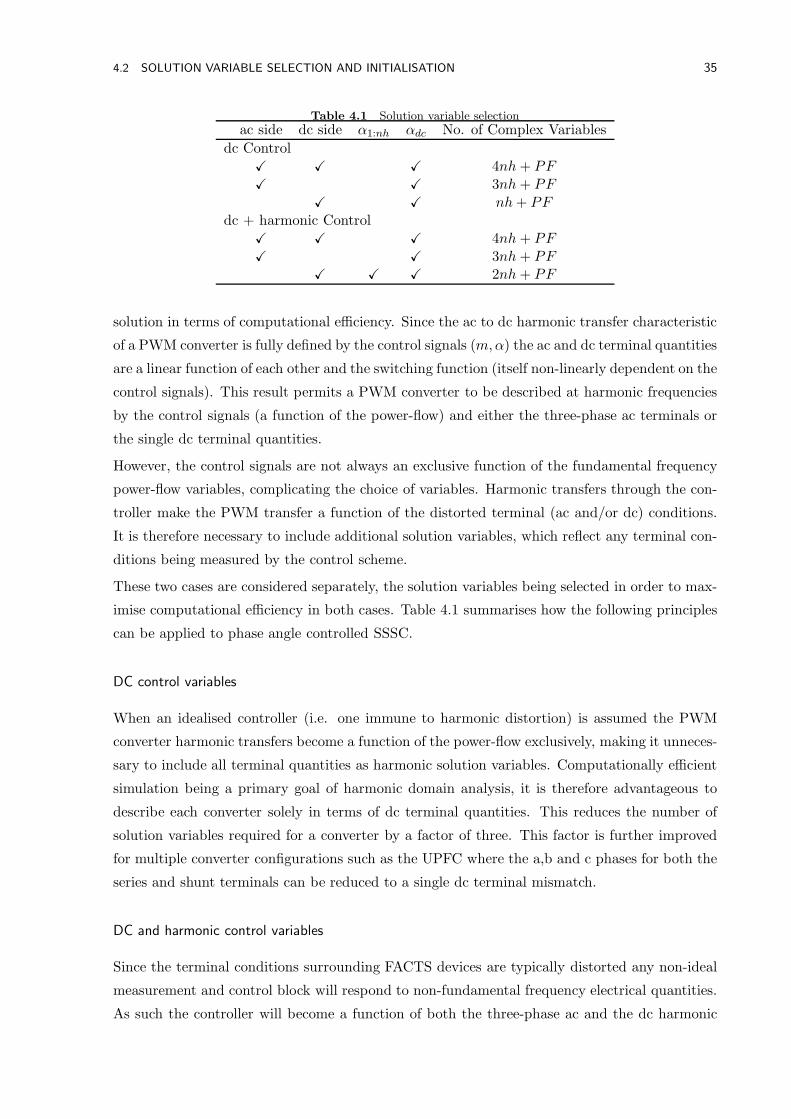
4.2 SOLUTION VARIABLE SELECTION AND INITIALISATION 35
Table 4.1 Solution variable selectionac side dc side α1:nh αdc No. of Complex Variables
dc ControlX X X 4nh+ PFX X 3nh+ PF
X X nh+ PFdc + harmonic Control
X X X 4nh+ PFX X 3nh+ PF
X X X 2nh+ PF
solution in terms of computational efficiency. Since the ac to dc harmonic transfer characteristic
of a PWM converter is fully defined by the control signals (m,α) the ac and dc terminal quantities
are a linear function of each other and the switching function (itself non-linearly dependent on the
control signals). This result permits a PWM converter to be described at harmonic frequencies
by the control signals (a function of the power-flow) and either the three-phase ac terminals or
the single dc terminal quantities.
However, the control signals are not always an exclusive function of the fundamental frequency
power-flow variables, complicating the choice of variables. Harmonic transfers through the con-
troller make the PWM transfer a function of the distorted terminal (ac and/or dc) conditions.
It is therefore necessary to include additional solution variables, which reflect any terminal con-
ditions being measured by the control scheme.
These two cases are considered separately, the solution variables being selected in order to max-
imise computational efficiency in both cases. Table 4.1 summarises how the following principles
can be applied to phase angle controlled SSSC.
DC control variables
When an idealised controller (i.e. one immune to harmonic distortion) is assumed the PWM
converter harmonic transfers become a function of the power-flow exclusively, making it unneces-
sary to include all terminal quantities as harmonic solution variables. Computationally efficient
simulation being a primary goal of harmonic domain analysis, it is therefore advantageous to
describe each converter solely in terms of dc terminal quantities. This reduces the number of
solution variables required for a converter by a factor of three. This factor is further improved
for multiple converter configurations such as the UPFC where the a,b and c phases for both the
series and shunt terminals can be reduced to a single dc terminal mismatch.
DC and harmonic control variables
Since the terminal conditions surrounding FACTS devices are typically distorted any non-ideal
measurement and control block will respond to non-fundamental frequency electrical quantities.
As such the controller will become a function of both the three-phase ac and the dc harmonic
36 CHAPTER 4 A UNIFIED SOLUTION TECHNIQUE
terminal conditions (assuming a regulated dc busbar scheme is used); its output containing a
portion of the terminal distortion present. Including all these quantities as solution variables
would cause a massive increase in the number of harmonic mismatches and the size of the
Jacobian, reducing computational efficiency.
The reduction in efficiency can be lessened by choosing the control ripple signals as the addi-
tional extra harmonic variables, rather than the ac terminal values. This is possible since (for
simplistic PI controllers) each control block is dependent on a single harmonic vector variable
(e.g. I+, V +, P , Q etc.), making it more efficient to choose the ac side solution variable after
the measurement block (e.g. dq transformation, P or Q calculation). Each PI controller can
therefore be characterised by a distorted control signal (e.g. α or m) updated with a positive
sequence mismatch 1.
When used in combination with the previously described dc variable formulation a wide variety
of basic ac and dc control schemes can be incorporated without the associated large increase in
the number of solution variables / mismatches.
4.2.2 Solution variable initialisation
To achieve reliable convergence it is critical that the solution variables are suitably initialised,
in particular the fundamental frequency operating point for each PWM converter. While it is
possible to initialise the system with a flat voltage profile and no harmonic distortion and then
solve the system using the full solution immediately, this is highly inefficient since each full
iteration is computationally intensive.
The solution variables are therefore initialised using the three-phase power-flow solved with no
harmonics included. When convergence is achieved the harmonic solution is added with all
harmonics initialised to zero. This point typically generates an adequate estimate of the full
Jacobian; making it unnecessary to re-calculate the Jacobian at subsequent iterations, while
still achieving satisfactory convergence.
4.3 POWER-FLOW SOLUTION
The harmonic performance of a converter is extremely dependent on the operating point of the
system to which it is connected, this necessitates the incorporation of fundamental frequency
operating point variation within the solution. A basic three-phase power-flow, the predominant
tool for this type of analysis, is used to fulfill this requirement.
Traditional PQ (load), PV (generator) and Slack buses are used in conjunction with a three-phase
adaptation of Canizares positive sequence FACTS device power-flow models [59] to represent the
1If the control scheme regulates both positive and negative sequence ac quantities it becomes necessary toinclude two harmonic control vectors of length nh, one for each sequence component. This makes it more straight-forward, and equally as efficient, to use the three ac terminals as the solution variables.
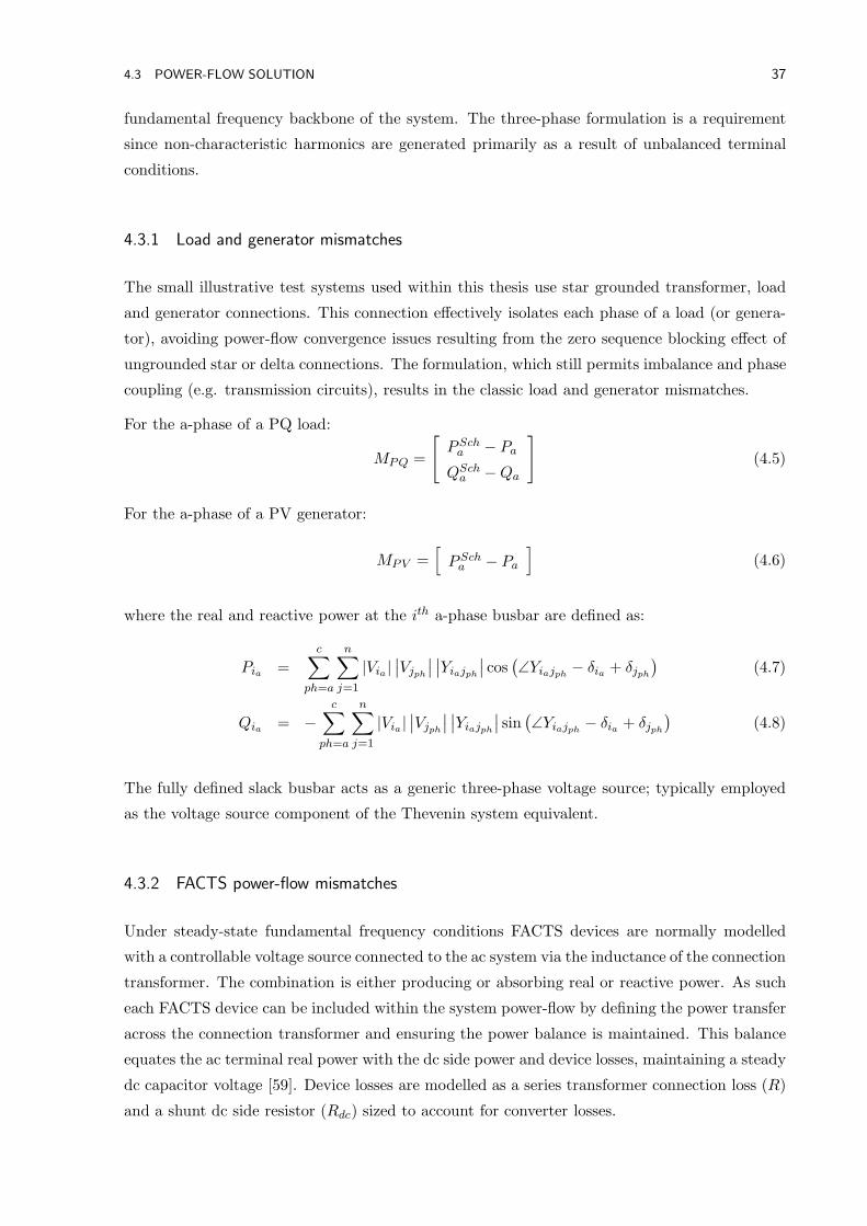
4.3 POWER-FLOW SOLUTION 37
fundamental frequency backbone of the system. The three-phase formulation is a requirement
since non-characteristic harmonics are generated primarily as a result of unbalanced terminal
conditions.
4.3.1 Load and generator mismatches
The small illustrative test systems used within this thesis use star grounded transformer, load
and generator connections. This connection effectively isolates each phase of a load (or genera-
tor), avoiding power-flow convergence issues resulting from the zero sequence blocking effect of
ungrounded star or delta connections. The formulation, which still permits imbalance and phase
coupling (e.g. transmission circuits), results in the classic load and generator mismatches.
For the a-phase of a PQ load:
MPQ =
[
PScha − Pa
QScha −Qa
]
(4.5)
For the a-phase of a PV generator:
MPV =[
PScha − Pa
]
(4.6)
where the real and reactive power at the ith a-phase busbar are defined as:
Pia =c∑
ph=a
n∑
j=1
|Via |∣∣Vjph
∣∣∣∣Yiajph
∣∣ cos
(∠Yiajph − δia + δjph
)(4.7)
Qia = −
c∑
ph=a
n∑
j=1
|Via |∣∣Vjph
∣∣∣∣Yiajph
∣∣ sin
(∠Yiajph − δia + δjph
)(4.8)
The fully defined slack busbar acts as a generic three-phase voltage source; typically employed
as the voltage source component of the Thevenin system equivalent.
4.3.2 FACTS power-flow mismatches
Under steady-state fundamental frequency conditions FACTS devices are normally modelled
with a controllable voltage source connected to the ac system via the inductance of the connection
transformer. The combination is either producing or absorbing real or reactive power. As such
each FACTS device can be included within the system power-flow by defining the power transfer
across the connection transformer and ensuring the power balance is maintained. This balance
equates the ac terminal real power with the dc side power and device losses, maintaining a steady
dc capacitor voltage [59]. Device losses are modelled as a series transformer connection loss (R)
and a shunt dc side resistor (Rdc) sized to account for converter losses.
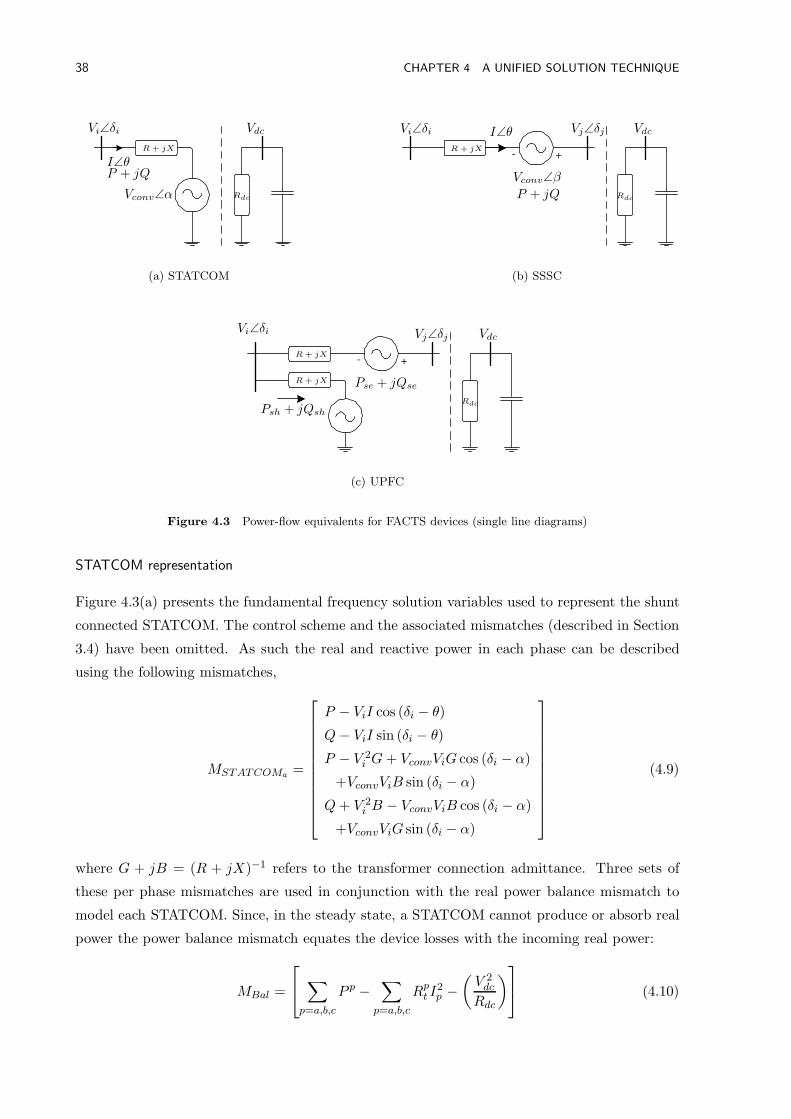
38 CHAPTER 4 A UNIFIED SOLUTION TECHNIQUE
Vi∠δi
I∠θ
Vconv∠α
P + jQ
R + jX
Rdc
Vdc
(a) STATCOM
+ -
Vi∠δi I∠θ
P + jQ
R + jX
Rdc
VdcVj∠δj
Vconv∠β
(b) SSSC
+ -
Vi∠δi
R + jX
R + jX
Rdc
VdcVj∠δj
Pse + jQse
Psh + jQsh
(c) UPFC
Figure 4.3 Power-flow equivalents for FACTS devices (single line diagrams)
STATCOM representation
Figure 4.3(a) presents the fundamental frequency solution variables used to represent the shunt
connected STATCOM. The control scheme and the associated mismatches (described in Section
3.4) have been omitted. As such the real and reactive power in each phase can be described
using the following mismatches,
MSTATCOMa =
P − ViI cos (δi − θ)
Q− ViI sin (δi − θ)
P − V 2i G+ VconvViG cos (δi − α)
+VconvViB sin (δi − α)
Q+ V 2i B − VconvViB cos (δi − α)
+VconvViG sin (δi − α)
(4.9)
where G + jB = (R + jX)−1 refers to the transformer connection admittance. Three sets of
these per phase mismatches are used in conjunction with the real power balance mismatch to
model each STATCOM. Since, in the steady state, a STATCOM cannot produce or absorb real
power the power balance mismatch equates the device losses with the incoming real power:
MBal =
∑
p=a,b,c
P p −∑
p=a,b,c
Rpt I2p −
(V 2dc
Rdc
)
(4.10)
4.3 POWER-FLOW SOLUTION 39
SSSC representation
The per phase power mismatches for a series connected SSSC (see Figure 4.3(b)) can be described
in a similar fashion to the STATCOM. The only significant difference is the requirement for an
additional set of PQ terminal mismatches,
MSSSCa =
Pi − ViI cos (δi − θ)
Qi − ViI sin (δi − θ)
Pj + VjI cos (δj − θ)
Qj + VjI sin (δj − θ)
P − (Pi + Pj)
Q− (Qi +Qj)
P − V 2G+ VconvV G cos (δ − β)
+VconvV B sin (δ − β)
Q+ V 2B − VconvV B cos (δ − β)
+VconvV G sin (δ − β)
(4.11)
where V ∠δ refers to the voltage difference between the ac terminal voltages Vi and Vj . The
power balance mismatch (Equation 4.10) remains unchanged for the SSSC.
UPFC representation
Given the hybrid nature of the UPFC (Figure 4.3(c)) it is modelled using a combination of
the shunt and series representations (Equations 4.9 and 4.11). However the power balance
mismatch must be generalised in order to permit real power transfers between the series and
shunt connections. This results in the following additional mismatches.
MBal =
(Psh + Pse) − (Pi + Pj)
(Qsh +Qse) − (Qi +Qj)∑
p=a,b,c
(P psh + P pse
)−
∑
p=a,b,c
(Rpsh(I
psh)
2 +Rpse(Ipse)2
)−
(V 2dc
Rdc
)
(4.12)
4.3.3 Power-flow dependence on harmonic solution variables
This power-flow representation is typically used in an isolated fashion, the impact of harmonics
being ignored. While this assumption is often adequate for fundamental frequency studies, it is
not strictly correct, nor is it appropriate for detailed harmonic studies. Since switching converters
can modulate harmonic frequency components at the dc terminal to fundamental frequency ac
quantities (and vice versa) the series or shunt voltage source equivalents become a function of
both fundamental and harmonic frequency variables.
Equations 4.9 and 4.11 have been included in a generalised fashion which can accommodate
either type of representation. The series or shunt voltage source (Vconv) can be defined as a
40 CHAPTER 4 A UNIFIED SOLUTION TECHNIQUE
function of the power-flow variables,
Vconv = kPWMmdcVdc(0Hz)∠αdc (4.13)
where kPWM is a constant relating the dc and ac voltage. It can also be defined as a function
of the dc voltage (Vdc including harmonics) and the switching function (itself a function of the
control variables).
Vconvph = Sph (α,m) ⊗ Vdc1:nh (4.14)
The fundamental frequency version is used for variable initialisation, while the convolutional
approach is adopted for the full harmonic solution.
4.4 HARMONIC SOLUTION
In contrast to the fundamental frequency power-flow, the majority of the harmonic system is
assumed to behave in a linear fashion, acting as a linear admittance over which non-linear
harmonic injections can interact. As such the harmonic mismatches are dependent on the ac
and dc system admittances, the operating point and the harmonic solution variables.
4.4.1 Linear ac system analysis
The ac system acts as the medium over which FACTS devices interact, making the ac system
impedance an integral part of the harmonic mismatches. Given the assumption that the re-
mainder of the ac system behaves in a linear fashion (at a given operating point), it is relatively
straightforward to incorporate using nodal analysis. This reduces the ac system to a harmonic
admittance matrix of the following form,
[
I1
I2
]
=
[
Y11 + Y12 −Y12
−Y12 Y22 + Y12
] [
V1
V2
]
(4.15)
where each branch of the equivalent-pi admittance (see Figure 3.14) is calculated or read from an
appropriate data file (for frequency dependent components) at all harmonics up to nh. The full
formation replicates Equation 4.15 for all three phases, including any phase to phase coupling
terms.
Since significant non-linear harmonic injections are only present at a small proportion of the
system nodes it is advantageous to eliminate passive busbars, improving computational efficiency.
Passive busbars are defined as linear busbars with no harmonic injection present, an example
being PQ busses, which are non-linear at fundamental frequency, but are represented as a fixed
impedance at harmonic frequencies. The resultant reduced system only contains the non-linear
FACTS harmonic injection busses, which are linked by equivalent impedances, as illustrated for
a two converter system system in Figure 4.4.
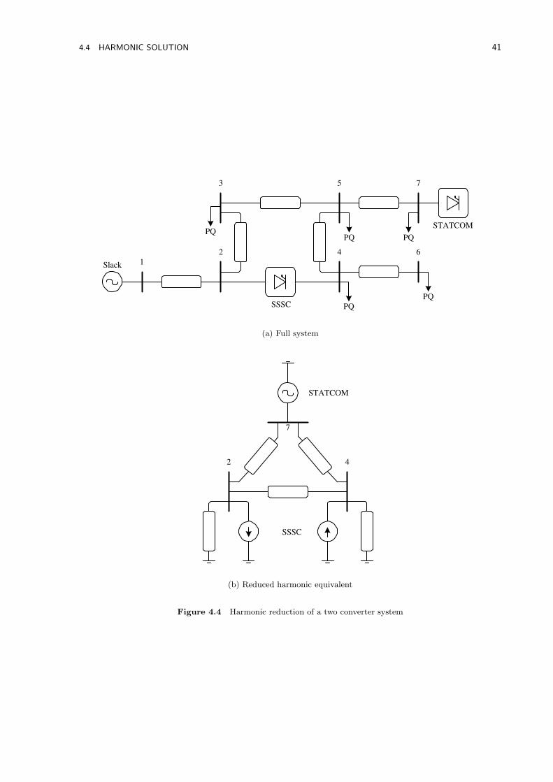
4.4 HARMONIC SOLUTION 41
PQ PQ
PQ
PQ STATCOM
SSSC PQ
Slack 1
2
3
4
5
6
7
(a) Full system
SSSC
2 4
7
STATCOM
(b) Reduced harmonic equivalent
Figure 4.4 Harmonic reduction of a two converter system
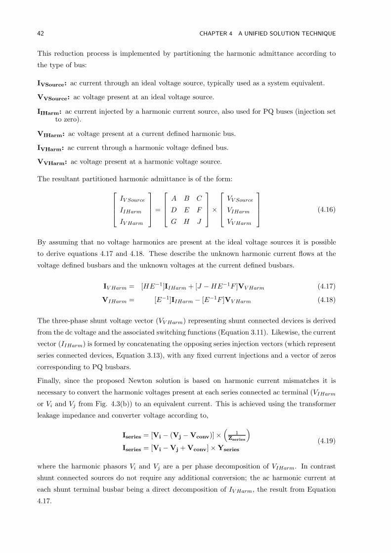
42 CHAPTER 4 A UNIFIED SOLUTION TECHNIQUE
This reduction process is implemented by partitioning the harmonic admittance according to
the type of bus:
IVSource: ac current through an ideal voltage source, typically used as a system equivalent.
VVSource: ac voltage present at an ideal voltage source.
IIHarm: ac current injected by a harmonic current source, also used for PQ buses (injection setto zero).
VIHarm: ac voltage present at a current defined harmonic bus.
IVHarm: ac current through a harmonic voltage defined bus.
VVHarm: ac voltage present at a harmonic voltage source.
The resultant partitioned harmonic admittance is of the form:
IV Source
IIHarm
IV Harm
=
A B C
D E F
G H J
×
VV Source
VIHarm
VV Harm
(4.16)
By assuming that no voltage harmonics are present at the ideal voltage sources it is possible
to derive equations 4.17 and 4.18. These describe the unknown harmonic current flows at the
voltage defined busbars and the unknown voltages at the current defined busbars.
IV Harm = [HE−1]IIHarm + [J −HE−1F ]VV Harm (4.17)
VIHarm = [E−1]IIHarm − [E−1F ]VV Harm (4.18)
The three-phase shunt voltage vector (VV Harm) representing shunt connected devices is derived
from the dc voltage and the associated switching functions (Equation 3.11). Likewise, the current
vector (IIHarm) is formed by concatenating the opposing series injection vectors (which represent
series connected devices, Equation 3.13), with any fixed current injections and a vector of zeros
corresponding to PQ busbars.
Finally, since the proposed Newton solution is based on harmonic current mismatches it is
necessary to convert the harmonic voltages present at each series connected ac terminal (VIHarm
or Vi and Vj from Fig. 4.3(b)) to an equivalent current. This is achieved using the transformer
leakage impedance and converter voltage according to,
Iseries = [Vi − (Vj − Vconv)] ×(
1Zseries
)
Iseries = [Vi − Vj + Vconv] × Yseries
(4.19)
where the harmonic phasors Vi and Vj are a per phase decomposition of VIHarm. In contrast
shunt connected sources do not require any additional conversion; the ac harmonic current at
each shunt terminal busbar being a direct decomposition of IV Harm, the result from Equation
4.17.
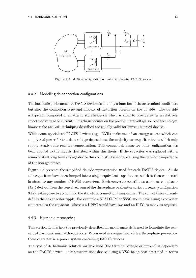
4.4 HARMONIC SOLUTION 43
Converter 1
Converter i
AC
System
V dc
+
-
R dc
C
I dc 1
I dc i
I dc Cap
Figure 4.5 dc Side configuration of multiple converter FACTS devices
4.4.2 Modelling dc connection configurations
The harmonic performance of FACTS devices is not only a function of the ac terminal conditions,
but also the connection type and amount of distortion present on the dc side. The dc side
is typically composed of an energy storage device which is sized to provide either a relatively
smooth dc voltage or current. This thesis focuses on the predominant voltage sourced technology,
however the analysis techniques described are equally valid for current sourced devices.
While some specialised FACTS devices (e.g. DVR) make use of an energy source which can
supply real power for transient voltage depressions, the majority use capacitor banks which only
supply steady-state reactive compensation. This common dc capacitor bank configuration has
been applied to the models described within this thesis. If the capacitor was replaced with a
semi-constant long term storage device this could still be modelled using the harmonic impedance
of the storage device.
Figure 4.5 presents the simplified dc side representation used for each FACTS device. All dc
side capacitors have been lumped into a single equivalent capacitance, which is then connected
in shunt to any number of PWM converters. Each converter contributes a dc current phasor
(Idci) derived from the convolved sum of the three-phase ac shunt or series currents (via Equation
3.12), taking care to account for the star-delta connection transformer. The sum of these currents
defines the dc capacitor ripple. For example a STATCOM or SSSC would have a single converter
connected to the capacitor, whereas a UPFC would have two and an IPFC as many as required.
4.4.3 Harmonic mismatches
This section details how the previously described harmonic analysis is used to formulate the real-
valued harmonic mismatch equations. When used in conjunction with a three-phase power-flow
these characterise a power system containing FACTS devices.
The type of dc harmonic solution variable used (the terminal voltage or current) is dependent
on the FACTS device under consideration; devices using a VSC being best described in terms
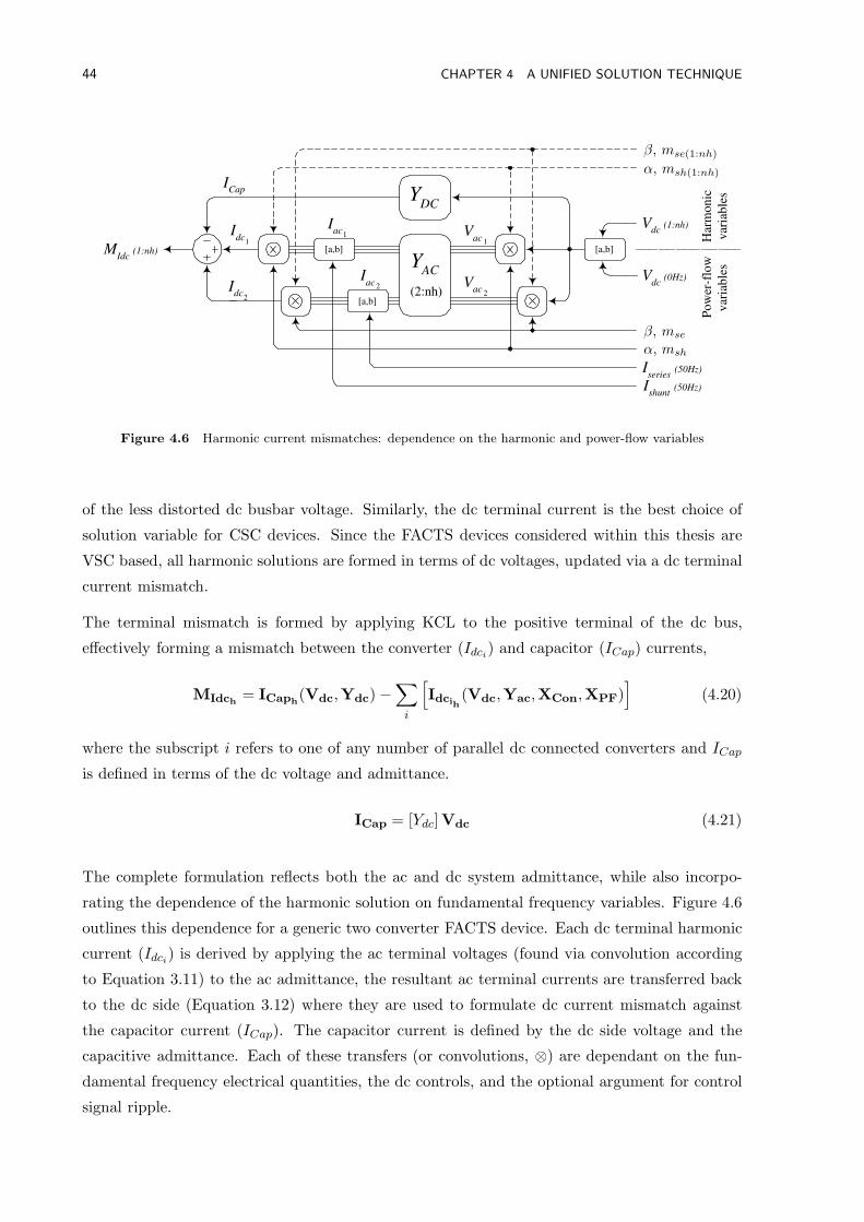
44 CHAPTER 4 A UNIFIED SOLUTION TECHNIQUE
V ac
I ac
Y AC
V dc
(1:nh)
Y DC
I Cap
I dc
M Idc
(1:nh)
V ac
I ac I
dc
V dc
(0Hz)
[a,b] [a,b]
(2:nh) [a,b]
I shunt
(50Hz)
I series
(50Hz)
Har
monic
var
iable
s
Pow
er-f
low
var
iable
s
1 1
1
2
2 2
β, mse
α, msh
β, mse(1:nh)
α, msh(1:nh)
Figure 4.6 Harmonic current mismatches: dependence on the harmonic and power-flow variables
of the less distorted dc busbar voltage. Similarly, the dc terminal current is the best choice of
solution variable for CSC devices. Since the FACTS devices considered within this thesis are
VSC based, all harmonic solutions are formed in terms of dc voltages, updated via a dc terminal
current mismatch.
The terminal mismatch is formed by applying KCL to the positive terminal of the dc bus,
effectively forming a mismatch between the converter (Idci) and capacitor (ICap) currents,
MIdch= ICaph
(Vdc,Ydc) −∑
i
[
Idcih
(Vdc,Yac,XCon,XPF)]
(4.20)
where the subscript i refers to one of any number of parallel dc connected converters and ICap
is defined in terms of the dc voltage and admittance.
ICap = [Ydc]Vdc (4.21)
The complete formulation reflects both the ac and dc system admittance, while also incorpo-
rating the dependence of the harmonic solution on fundamental frequency variables. Figure 4.6
outlines this dependence for a generic two converter FACTS device. Each dc terminal harmonic
current (Idci) is derived by applying the ac terminal voltages (found via convolution according
to Equation 3.11) to the ac admittance, the resultant ac terminal currents are transferred back
to the dc side (Equation 3.12) where they are used to formulate dc current mismatch against
the capacitor current (ICap). The capacitor current is defined by the dc side voltage and the
capacitive admittance. Each of these transfers (or convolutions, ⊗) are dependant on the fun-
damental frequency electrical quantities, the dc controls, and the optional argument for control
signal ripple.
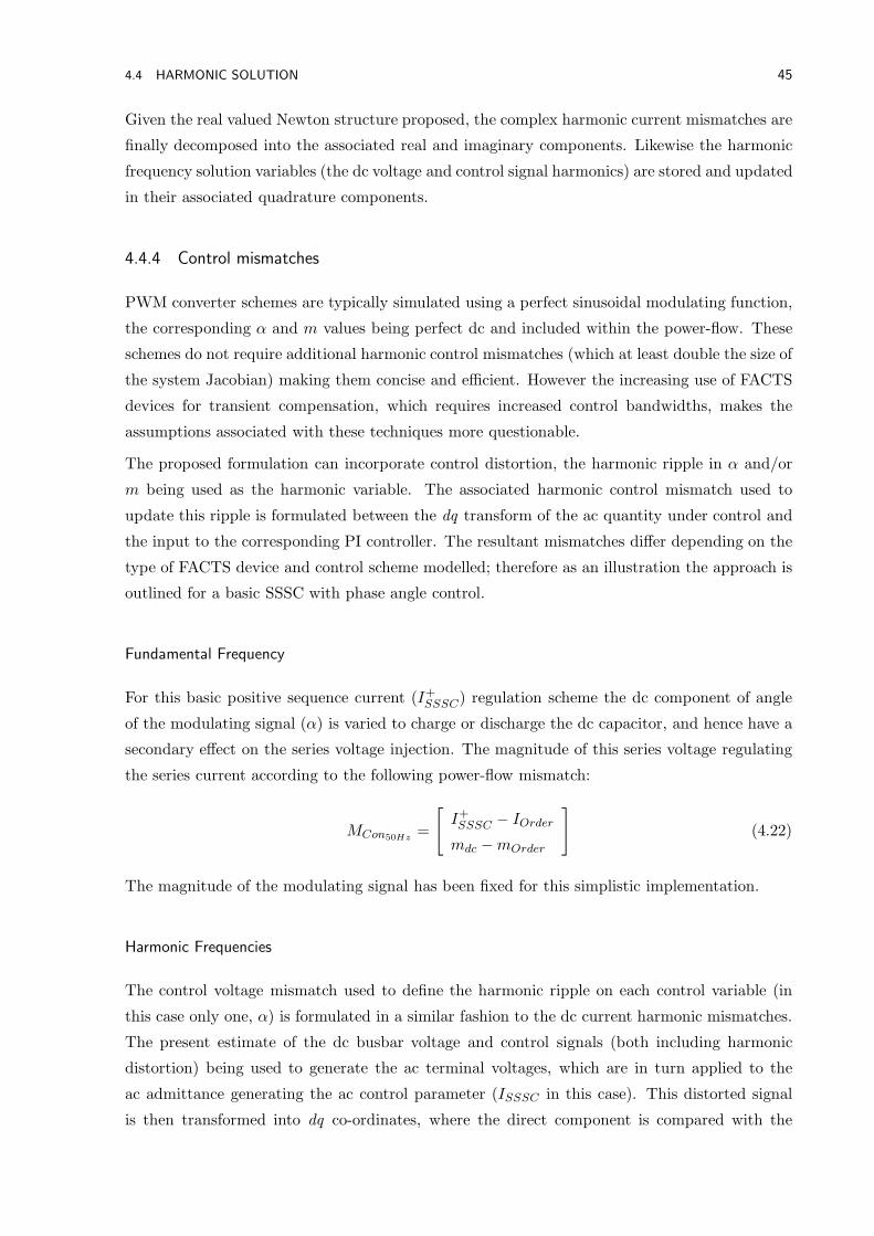
4.4 HARMONIC SOLUTION 45
Given the real valued Newton structure proposed, the complex harmonic current mismatches are
finally decomposed into the associated real and imaginary components. Likewise the harmonic
frequency solution variables (the dc voltage and control signal harmonics) are stored and updated
in their associated quadrature components.
4.4.4 Control mismatches
PWM converter schemes are typically simulated using a perfect sinusoidal modulating function,
the corresponding α and m values being perfect dc and included within the power-flow. These
schemes do not require additional harmonic control mismatches (which at least double the size of
the system Jacobian) making them concise and efficient. However the increasing use of FACTS
devices for transient compensation, which requires increased control bandwidths, makes the
assumptions associated with these techniques more questionable.
The proposed formulation can incorporate control distortion, the harmonic ripple in α and/or
m being used as the harmonic variable. The associated harmonic control mismatch used to
update this ripple is formulated between the dq transform of the ac quantity under control and
the input to the corresponding PI controller. The resultant mismatches differ depending on the
type of FACTS device and control scheme modelled; therefore as an illustration the approach is
outlined for a basic SSSC with phase angle control.
Fundamental Frequency
For this basic positive sequence current (I+SSSC) regulation scheme the dc component of angle
of the modulating signal (α) is varied to charge or discharge the dc capacitor, and hence have a
secondary effect on the series voltage injection. The magnitude of this series voltage regulating
the series current according to the following power-flow mismatch:
MCon50Hz=
[
I+SSSC − IOrder
mdc −mOrder
]
(4.22)
The magnitude of the modulating signal has been fixed for this simplistic implementation.
Harmonic Frequencies
The control voltage mismatch used to define the harmonic ripple on each control variable (in
this case only one, α) is formulated in a similar fashion to the dc current harmonic mismatches.
The present estimate of the dc busbar voltage and control signals (both including harmonic
distortion) being used to generate the ac terminal voltages, which are in turn applied to the
ac admittance generating the ac control parameter (ISSSC in this case). This distorted signal
is then transformed into dq co-ordinates, where the direct component is compared with the

46 CHAPTER 4 A UNIFIED SOLUTION TECHNIQUE
V ac
I ac
Y AC
V dc
(1:nh) M Con
(1:nh)
V dc
(0Hz)
[a,b] [a,b]
I series
(50Hz)
Har
monic
var
iable
s
Pow
er-f
low
var
iable
s
( PI ) -1
d q
a b c
I Con +
I Sys +
α(1 : nh)
α, msh
Figure 4.7 Harmonic control mismatches: dependence on the harmonic and power-flow variables
input to the control block, derived from the control variable ripple and the inverse PI control
characteristic.
MConh= IdSysh
(Vdc,XCon,XPF) − IdConh(XCon,PI) (4.23)
IdSysh refers to the positive sequence estimate (via the dq transform) of the series current, and
IdConh is the same quantity calculated via the PI controller block. Figure 4.7 outlines this
process, highlighting the interdependence with the power-flow variables. Note how the phase
angle reference for the dq transformation is idealised, and hence provided by the power-flow
rather than via a PLL (for which the angle reference would be a function of the harmonic
variables).
4.5 SYSTEM JACOBIAN FORMULATION
The final critical component of the harmonic solution system is the system Jacobian, a matrix
of partial derivatives representing the case specific linearisation for a system. This linearisa-
tion is both relatively complex to derive analytically and computationally expensive to derive
numerically, making it the critical determinant of the models flexibility and efficiency.
4.5.1 Jacobian derivation
While analytic derivation of the system Jacobian has been shown to be an efficient and practical
method for HVdc converters [10, 34] it is not necessarily as applicable to PWM converters. PWM
converters differ from 6 or 12 pulse line commutated devices in that the number of switching
instants can vary with the operating point. Over-modulation (where the magnitude of m exceeds
that of Vtri) leads to a reduction in the number of switching instants and a discontinuity in δψδm ,
making analytic Jacobian derivation more difficult.
In contrast numerical derivation of the Jacobian, while computationally expensive, can be easily
applied to generalised PWM systems containing multiple switching frequencies and modulation

4.5 SYSTEM JACOBIAN FORMULATION 47
indices. Further, numerical derivation of the Jacobian is straightforward to formulate, can be
extended in a modular fashion, and is robust. A numerical Jacobian is calculated by simply
sequentially perturbing each of the solution variables, and observing the change in the resultant
mismatch vector. This difference vector is then divided by the magnitude of the perturba-
tion, generating one column of the Jacobian. In order for this approximation to be valid the
perturbation must be small enough such that:
J =δF
δx≈F (x+ ∆x) − F (x)
∆x(4.24)
Numerical derivation has therefore been adopted so as to maintain generality at the cost of
computational efficiency. A perturbation magnitude of 10−6 pu has been applied to the funda-
mental frequency (distortion free) operating point; this technique has been shown experimentally
to provide a satisfactory estimate of the full harmonic Jacobian.
4.5.2 Jacobian structure
Block structure: dc control variables
Regardless of its derivation, the structure of the Jacobian is defined by the test system and the
choice of solution variables. Each variable is related to a column of dependent mismatches by
the Jacobian. For a basic fundamental frequency controller this structure is relatively simple,
the unified solution being defined in terms of the power-flow variables (XPF ) and a single dc
voltage phasor (Vdc) for each FACTS device.
The resulting Jacobian therefore contains a power-flow block ( δMPF
δXPF), diagonal harmonic blocks
for each FACTS device (δMIdci
δVdci), and off-diagonal mutual coupling blocks. Each of these harmonic
blocks has a lattice structure corresponding to converter frequency transfers, themselves function
of the PWM switching frequency. As such the Jacobian for a system containing two FACTS
devices is of the form of Equation 4.25, a numerically derived example being included in Figure
4.8(a).
MPF
MIdc1
MIdc2
=
δMPF
δXPFδMPF
δVdc1δMPF
δVdc2δMIdc1
δXPF
δMIdc1
δVdc1
δMIdc1
δVdc2δMIdc2
δXPF
δMIdc2
δVdc1
δMIdc2
δVdc2
∆XPF
∆Vdc1
∆Vdc2
(4.25)
The real and imaginary component of each dc voltage harmonic (and the associated mismatch)
are treated as separate solution variables. The real valued Jacobian elements relating these
variables are therefore 2 × 2 tensors [10], having the form of Equation 4.26.
[
ℜ(MIdc)
ℑ(MIdc)
]
=
[
J11 J12
J21 J22
]
·
[
∆ℜ(Vdc)
∆ℑ(Vdc)
]
(4.26)
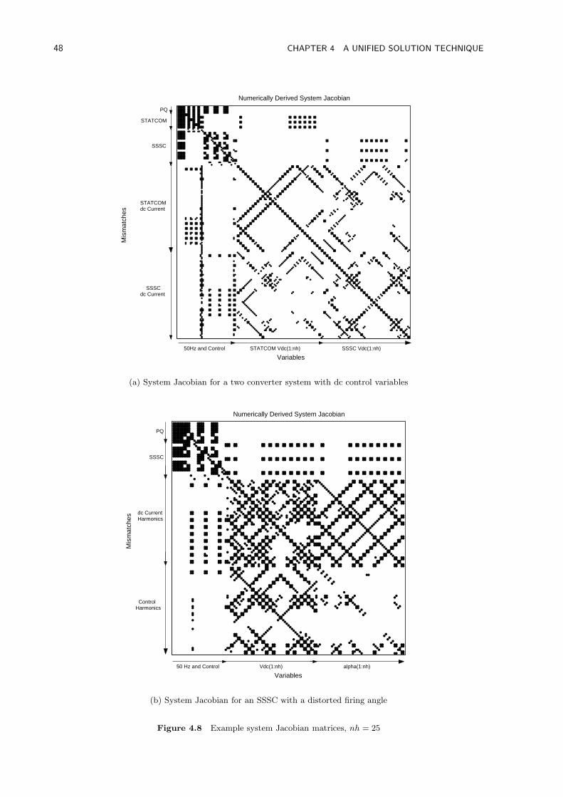
48 CHAPTER 4 A UNIFIED SOLUTION TECHNIQUE
Numerically Derived System Jacobian
Mis
mat
ches
Variables
PQ
STATCOM
SSSC
STATCOMdc Current
SSSCdc Current
50Hz and Control STATCOM Vdc(1:nh) SSSC Vdc(1:nh)
(a) System Jacobian for a two converter system with dc control variables
Numerically Derived System Jacobian
Mis
mat
ches
Variables
PQ
SSSC
dc CurrentHarmonics
ControlHarmonics
50 Hz and Control Vdc(1:nh) alpha(1:nh)
(b) System Jacobian for an SSSC with a distorted firing angle
Figure 4.8 Example system Jacobian matrices, nh = 25
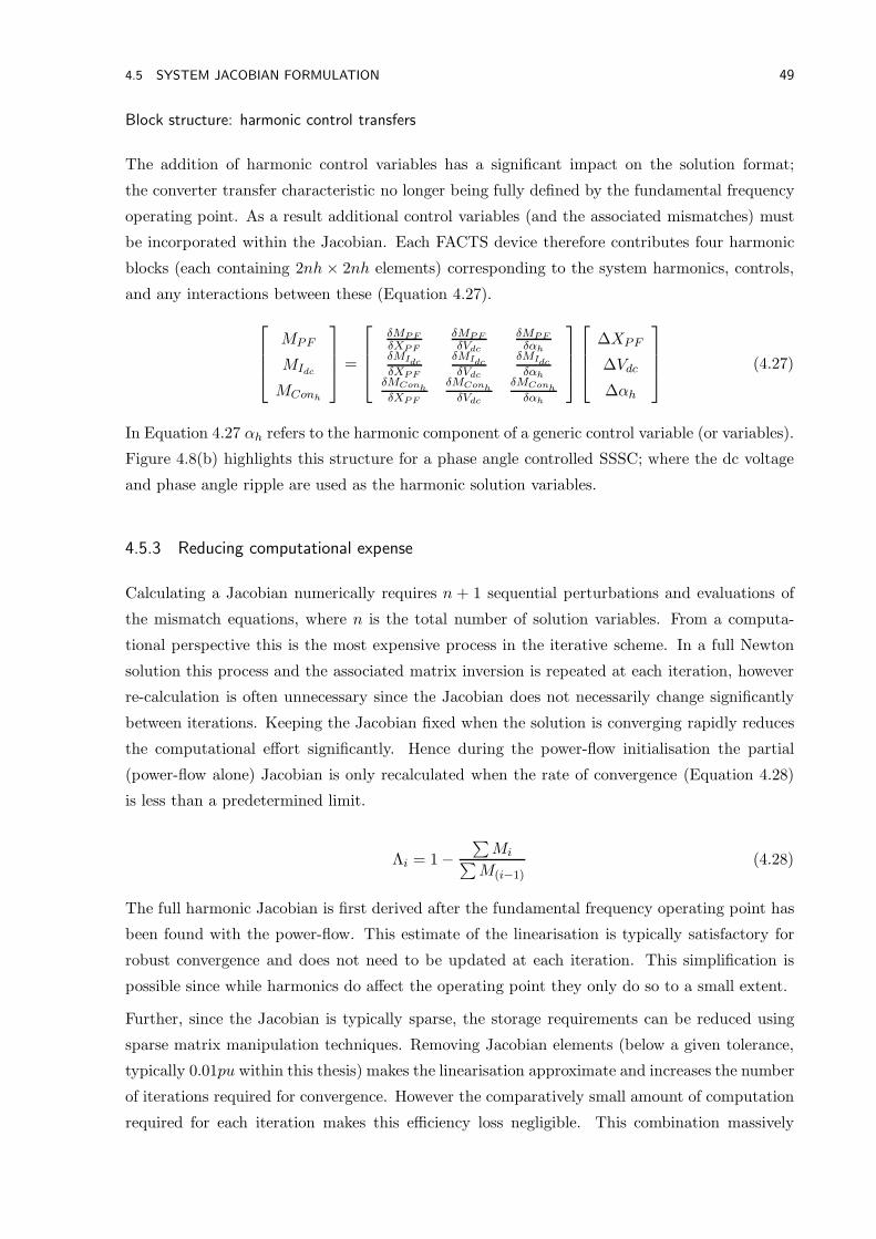
4.5 SYSTEM JACOBIAN FORMULATION 49
Block structure: harmonic control transfers
The addition of harmonic control variables has a significant impact on the solution format;
the converter transfer characteristic no longer being fully defined by the fundamental frequency
operating point. As a result additional control variables (and the associated mismatches) must
be incorporated within the Jacobian. Each FACTS device therefore contributes four harmonic
blocks (each containing 2nh × 2nh elements) corresponding to the system harmonics, controls,
and any interactions between these (Equation 4.27).
MPF
MIdc
MConh
=
δMPF
δXPFδMPF
δVdcδMPF
δαhδMIdc
δXPF
δMIdc
δVdc
δMIdc
δαhδMConh
δXPF
δMConh
δVdc
δMConh
δαh
∆XPF
∆Vdc
∆αh
(4.27)
In Equation 4.27 αh refers to the harmonic component of a generic control variable (or variables).
Figure 4.8(b) highlights this structure for a phase angle controlled SSSC; where the dc voltage
and phase angle ripple are used as the harmonic solution variables.
4.5.3 Reducing computational expense
Calculating a Jacobian numerically requires n + 1 sequential perturbations and evaluations of
the mismatch equations, where n is the total number of solution variables. From a computa-
tional perspective this is the most expensive process in the iterative scheme. In a full Newton
solution this process and the associated matrix inversion is repeated at each iteration, however
re-calculation is often unnecessary since the Jacobian does not necessarily change significantly
between iterations. Keeping the Jacobian fixed when the solution is converging rapidly reduces
the computational effort significantly. Hence during the power-flow initialisation the partial
(power-flow alone) Jacobian is only recalculated when the rate of convergence (Equation 4.28)
is less than a predetermined limit.
Λi = 1 −
∑Mi
∑M(i−1)
(4.28)
The full harmonic Jacobian is first derived after the fundamental frequency operating point has
been found with the power-flow. This estimate of the linearisation is typically satisfactory for
robust convergence and does not need to be updated at each iteration. This simplification is
possible since while harmonics do affect the operating point they only do so to a small extent.
Further, since the Jacobian is typically sparse, the storage requirements can be reduced using
sparse matrix manipulation techniques. Removing Jacobian elements (below a given tolerance,
typically 0.01pu within this thesis) makes the linearisation approximate and increases the number
of iterations required for convergence. However the comparatively small amount of computation
required for each iteration makes this efficiency loss negligible. This combination massively
50 CHAPTER 4 A UNIFIED SOLUTION TECHNIQUE
reduces the amount of computation required to reach convergence since only the smaller power-
flow Jacobian is recalculated, while the massive harmonic Jacobian is only formulated once and
handled using sparse routines.
4.6 MODEL EXTENSION TO OTHER NON-LINEAR DEVICES
If under given operating conditions a system component is deemed to be unsatisfactorily ap-
proximated using linearised analysis, additional non-linear models could be incorporated within
the proposed formulation. Each additional non-linear component would need to be defined as
either a harmonic current or voltage source each of which would be a function of a further set of
solution variables. The dc side FACTS formulation makes any combined representation some-
what less intuitive, since the system would be composed of a combination of ac and dc ports,
but does not limit the addition of further ac side non-linear injections.
The additional accuracy which could be obtained by using more advanced component models
needs to be balanced against the increase in computational expense and the accuracy of system
data at harmonic frequencies. Given the lack of harmonic information pertaining to system
loads and transmission lines it is uncertain whether the possible gain in accuracy merits the
associated reduction in efficiency.
4.7 CONCLUSIONS
This chapter has presented a generalised harmonic domain algorithm capable of representing
hard-switched FACTS devices and the associated electrical systems, according to the models
described in Chapter 3. The formulation is based around a three-phase power-flow used in
conjunction with a harmonic representation. The harmonic solution reduces the linear ac and
dc systems to a dc side harmonic equivalent for each FACTS device. This cuts the number
of solution variables and reduces the size and computational expense of deriving the system
Jacobian. This principle is applicable to a variety of ac and dc connection topologies with
multiple PWM converters, providing a comprehensive, yet efficient, harmonic representation.
Chapter 5
MODEL IMPLEMENTATION, VALIDATION AND PERFORMANCE
5.1 INTRODUCTION
This chapter presents the MATLAB implementation and validation for the proposed FACTS
device models. The models are applied to a basic 5-busbar test system containing a series
(SSSC) and shunt (STATCOM) connected PWM converter, the results being compared against
time domain simulation. The test system (see Figure 5.1 and Appendix B.1) is composed of a
deliberately over-simplified transmission network (a balanced series equivalent impedance), two
fixed impedance loads and a balanced Thevenin equivalent system representation. This system
avoids the modelling difficulties associated with the more advanced transmission representations
(see Section 6.2.2), making accurate validation of the proposed PWM converter model more
straightforward.
The computational efficiency aspects, which differentiate time and harmonic domain steady-
state analysis are considered, both in terms of the solution speed and convergence properties.
These properties are heavily dependent on the nature of the system Jacobian, which is explored
both as a visual measure of variable interaction and with the aim of improving model efficiency.
Finally the interaction between the operating point and the harmonic solution is discussed, with
reference to the advantages and disadvantages of using linearised analysis.
5.2 MODEL IMPLEMENTATION
5.2.1 Harmonic domain model
The proposed Newton solution was implemented within the MATLAB environment which, even
though it includes extra computational overheads, provides a versatile (if somewhat inefficient)
range of matrix handling functions. Of particular importance to harmonic analysis are the sparse
matrix handling and matrix inversion facilities which deal with the large harmonic admittance
and Jacobian matrices.
The program is structured to first form the harmonic and power-flow admittance matrices in
per phase and per unit terms, either from basic RLC branch data, or an external file containing
harmonic admittance data. These matrices are then re-structured according to Section 4.4.1,
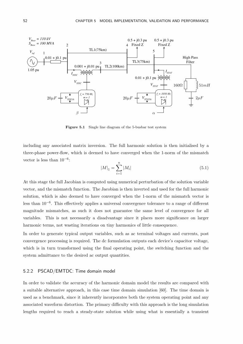
52 CHAPTER 5 MODEL IMPLEMENTATION, VALIDATION AND PERFORMANCE
I SSSC
0.001 + j0.01 pu
I STAT
TL1(75km)
TL2(100km)
0.01 + j0.1 pu
0.5 + j0.3 pu
Fixed Z
0.5 + j0.3 pu
Fixed Z
TL3(75km)
V inf
0.01 + j0.1 pu
1.05 pu
V Base
= 110 kV
S Base
= 100 MVA
V SSSC V
STAT
V STATdc
V SSSCdc
f s = 750 Hz
m = 1
f s = 1050 Hz
m = 1
1
2
3
4
5
High Pass
Filter
20µF
β
20µF
α
160Ω 51mH
2µF
Figure 5.1 Single line diagram of the 5-busbar test system
including any associated matrix inversion. The full harmonic solution is then initialised by a
three-phase power-flow, which is deemed to have converged when the 1-norm of the mismatch
vector is less than 10−6:
|M |1 =n∑
i=1
|Mi| (5.1)
At this stage the full Jacobian is computed using numerical perturbation of the solution variable
vector, and the mismatch function. The Jacobian is then inverted and used for the full harmonic
solution, which is also deemed to have converged when the 1-norm of the mismatch vector is
less than 10−6. This effectively applies a universal convergence tolerance to a range of different
magnitude mismatches, as such it does not guarantee the same level of convergence for all
variables. This is not necessarily a disadvantage since it places more significance on larger
harmonic terms, not wasting iterations on tiny harmonics of little consequence.
In order to generate typical output variables, such as ac terminal voltages and currents, post
convergence processing is required. The dc formulation outputs each device’s capacitor voltage,
which is in turn transformed using the final operating point, the switching function and the
system admittance to the desired ac output quantities.
5.2.2 PSCAD/EMTDC: Time domain model
In order to validate the accuracy of the harmonic domain model the results are compared with
a suitable alternative approach, in this case time domain simulation [60]. The time domain is
used as a benchmark, since it inherently incorporates both the system operating point and any
associated waveform distortion. The primary difficulty with this approach is the long simulation
lengths required to reach a steady-state solution while using what is essentially a transient
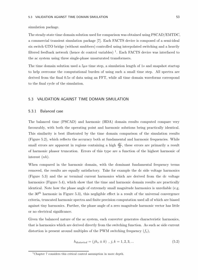
5.3 VALIDATION AGAINST TIME DOMAIN SIMULATION 53
simulation package.
The steady-state time domain solution used for comparison was obtained using PSCAD/EMTDC,
a commercial transient simulation package [7]. Each FACTS device is composed of a semi-ideal
six switch GTO bridge (without snubbers) controlled using interpolated switching and a heavily
filtered feedback network (hence dc control variables) 1. Each FACTS device was interfaced to
the ac system using three single-phase unsaturated transformers.
The time domain solution used a 5µs time step, a simulation length of 1s and snapshot startup
to help overcome the computational burden of using such a small time step. All spectra are
derived from the final 0.5s of data using an FFT, while all time domain waveforms correspond
to the final cycle of the simulation.
5.3 VALIDATION AGAINST TIME DOMAIN SIMULATION
5.3.1 Balanced case
The balanced time (PSCAD) and harmonic (HDA) domain results computed compare very
favourably, with both the operating point and harmonic solutions being practically identical.
This similarity is best illustrated by the time domain comparison of the simulation results
(Figure 5.2), which reflects the accuracy both at fundamental and harmonic frequencies. While
small errors are apparent in regions containing a high dVdt , these errors are primarily a result
of harmonic phasor truncation. Errors of this type are a function of the highest harmonic of
interest (nh).
When compared in the harmonic domain, with the dominant fundamental frequency terms
removed, the results are equally satisfactory. Take for example the dc side voltage harmonics
(Figure 5.3) and the ac terminal current harmonics which are derived from the dc voltage
harmonics (Figure 5.4), which show that the time and harmonic domain results are practically
identical. Note how the phase angle of extremely small magnitude harmonics is unreliable (e.g.
the 30th harmonic in Figure 5.3), this negligible effect is a result of the universal convergence
criteria, truncated harmonic spectra and finite precision computation used all of which are biased
against tiny harmonics. Further, the phase angle of a zero magnitude harmonic vector has little
or no electrical significance.
Given the balanced nature of the ac system, each converter generates characteristic harmonics,
that is harmonics which are derived directly from the switching function. As such ac side current
distortion is present around multiples of the PWM switching frequency (fs),
hdistorted = (jhs ± k) , j, k = 1, 2, 3, ... (5.2)
1Chapter 7 considers this critical control assumption in more depth.
54 CHAPTER 5 MODEL IMPLEMENTATION, VALIDATION AND PERFORMANCE
0 1 2 3 4 5 60.05
0.1
0.15
0.2
0.25S
SS
C d
c vo
ltgae
(pu
)
0 1 2 3 4 5 6−1
−0.5
0
0.5
1
Angle (rads)
SS
SC
ac
curr
ent ’
a’ (
pu)
HDAPSCAD
(a) SSSC results
0 1 2 3 4 5 60.85
0.86
0.87
0.88
0.89
0.9
ST
AT
CO
M d
c vo
ltage
(pu
)
0 1 2 3 4 5 6−1
−0.5
0
0.5
1
Angle (rads)
ST
AT
CO
M a
c cu
rren
t ’a’
(pu
)
HDAPSCAD
(b) STATCOM results
Figure 5.2 Time domain comparison for the balanced system
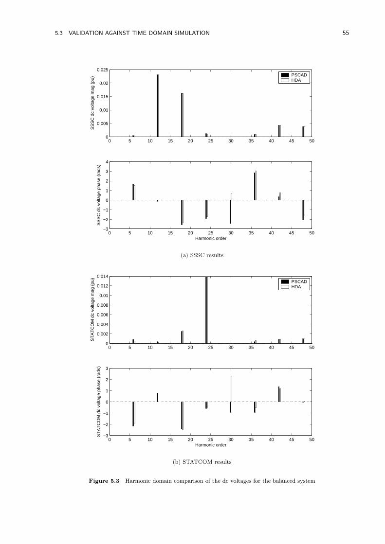
5.3 VALIDATION AGAINST TIME DOMAIN SIMULATION 55
0 5 10 15 20 25 30 35 40 45 500
0.005
0.01
0.015
0.02
0.025
SS
SC
dc
volta
ge m
ag (
pu)
0 5 10 15 20 25 30 35 40 45 50−3
−2
−1
0
1
2
3
4
Harmonic order
SS
SC
dc
volta
ge p
hase
(ra
ds)
PSCADHDA
(a) SSSC results
0 5 10 15 20 25 30 35 40 45 500
0.002
0.004
0.006
0.008
0.01
0.012
0.014
ST
AT
CO
M d
c vo
ltage
mag
(pu
)
0 5 10 15 20 25 30 35 40 45 50−3
−2
−1
0
1
2
3
Harmonic order
ST
AT
CO
M d
c vo
ltage
pha
se (
rads
)
PSCADHDA
(b) STATCOM results
Figure 5.3 Harmonic domain comparison of the dc voltages for the balanced system
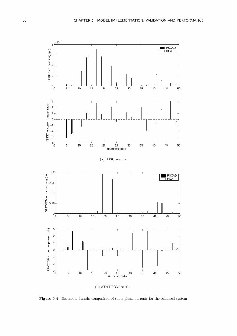
56 CHAPTER 5 MODEL IMPLEMENTATION, VALIDATION AND PERFORMANCE
0 5 10 15 20 25 30 35 40 45 500
2
4
6
8x 10
−3
SS
SC
ac
curr
ent m
ag (
pu)
0 5 10 15 20 25 30 35 40 45 50−4
−3
−2
−1
0
1
2
3
Harmonic order
SS
SC
ac
curr
ent p
hase
(ra
ds)
PSCADHDA
(a) SSSC results
0 5 10 15 20 25 30 35 40 45 500
0.05
0.1
0.15
0.2
ST
AT
CO
M a
c cu
rren
t mag
(pu
)
0 5 10 15 20 25 30 35 40 45 50−3
−2
−1
0
1
2
3
Harmonic order
ST
AT
CO
M a
c cu
rren
t pha
se (
rads
)
PSCADHDA
(b) STATCOM results
Figure 5.4 Harmonic domain comparison of the a-phase currents for the balanced system
5.4 MODEL PERFORMANCE 57
where
hs =fsf1. (5.3)
This is particularly evident in the ac current spectra for the STATCOM (hs = 21), which has
dominant terms at hs ± 2 and 2hs ± 1 (i.e. 19th,23rd,41st and 43rd harmonics). These textbook
characteristic spectra are complicated by the presence of the other converters’ characteristic
harmonics which are coupled, to differing extents, through the ac system. The magnitude of the
interaction is a function of the converters’ respective operating points, in this case the relatively
small series injection (Vseries ∼ 0.1pu) does not rival the dominance of the shunt injection
(Vshunt ∼ 1pu). Hence the ac current spectra for the SSSC has large spectral components
derived from the STATCOM’s characteristic distortion, whereas the STATCOM current is almost
exclusively a function of its own converter.
5.3.2 Unbalanced case
The presence of system imbalance leads to the generation of additional non-characteristic har-
monics, these require either a three-phase or positive/negative sequence approach. To test the
proposed method, which reflects a full three-phase formulation in the dc side variables, a grossly
exaggerated imbalance in the leakage impedance of the connection transformer was included.
This amounted to a 50% increase in the a-phase impedance for the STATCOM and the b-phase
impedance for the SSSC. The result is a 5% negative sequence current imbalance at the STAT-
COM and a very small imbalance in the SSSC current (since the series transformer leakage
impedance is small in comparison with the line impedances).
This imbalance does not result in any significant degradation in the quality of the match be-
tween the two simulation techniques, the time domain results still being almost indistinguishable
(Figure 5.5). Likewise, the frequency domain comparison of the dc voltages shows good agree-
ment (Figure 5.6). The dc voltage now contains a slew of small uncharacteristic harmonic terms
and a large second harmonic component. This second harmonic component is reflected in the
ac terminal currents as a third harmonic component, now present in both converters spectra
(Figure 5.7).
5.4 MODEL PERFORMANCE
5.4.1 Convergence properties
While accurate agreement with PSCAD/EMTDC is important, this in itself does not advance
harmonic analysis. Equally critical is the rate and manner in which convergence is achieved.
In general, given appropriate power-flow initialisation, the proposed harmonic model reliably
converges to a solution consistent with time domain simulation using PSCAD/EMTDC. The rate
of convergence is dependent on the type of system being simulated, in particular the number
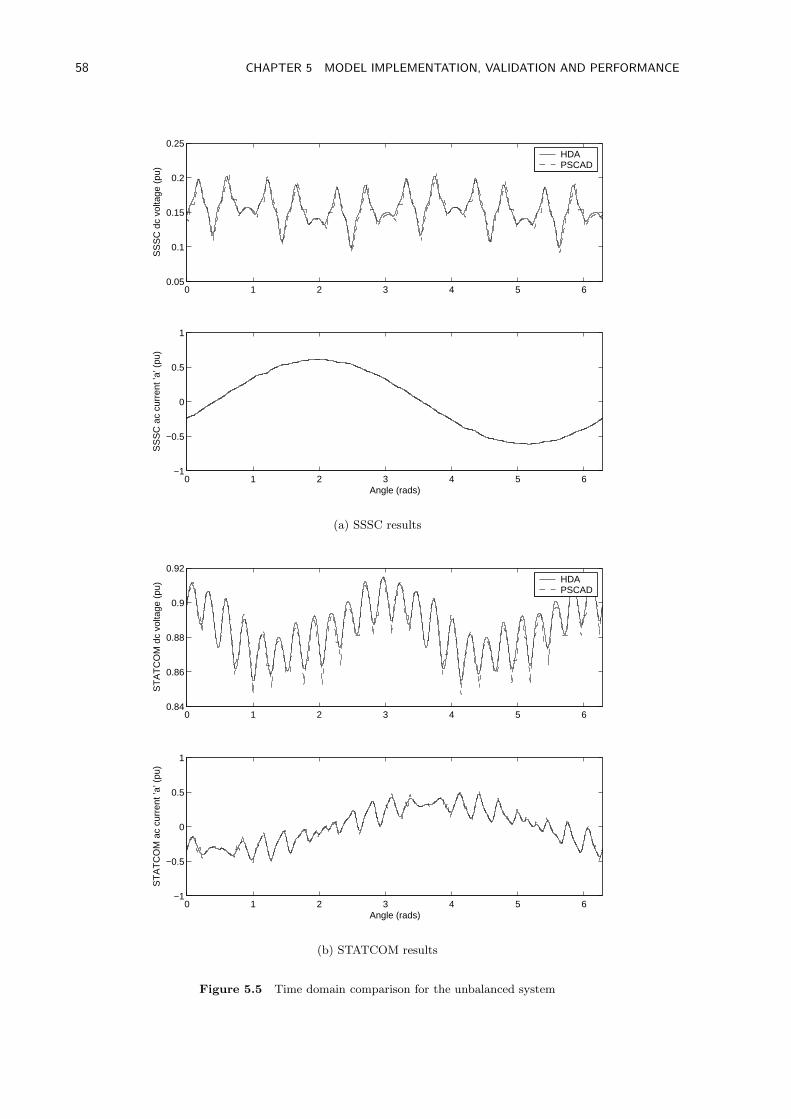
58 CHAPTER 5 MODEL IMPLEMENTATION, VALIDATION AND PERFORMANCE
0 1 2 3 4 5 60.05
0.1
0.15
0.2
0.25S
SS
C d
c vo
ltage
(pu
)
0 1 2 3 4 5 6−1
−0.5
0
0.5
1
Angle (rads)
SS
SC
ac
curr
ent ’
a’ (
pu)
HDAPSCAD
(a) SSSC results
0 1 2 3 4 5 60.84
0.86
0.88
0.9
0.92
ST
AT
CO
M d
c vo
ltage
(pu
)
0 1 2 3 4 5 6−1
−0.5
0
0.5
1
Angle (rads)
ST
AT
CO
M a
c cu
rren
t ’a’
(pu
)
HDAPSCAD
(b) STATCOM results
Figure 5.5 Time domain comparison for the unbalanced system
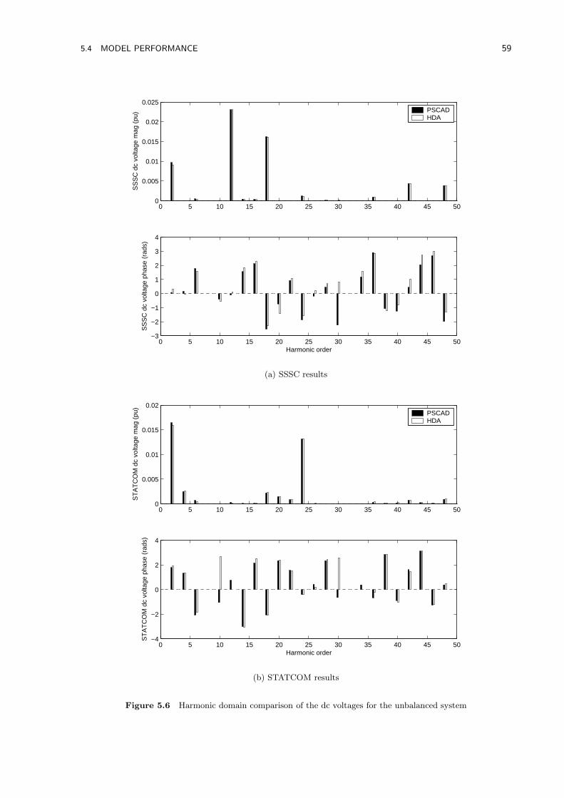
5.4 MODEL PERFORMANCE 59
0 5 10 15 20 25 30 35 40 45 500
0.005
0.01
0.015
0.02
0.025
SS
SC
dc
volta
ge m
ag (
pu)
0 5 10 15 20 25 30 35 40 45 50−3
−2
−1
0
1
2
3
4
Harmonic order
SS
SC
dc
volta
ge p
hase
(ra
ds)
PSCADHDA
(a) SSSC results
0 5 10 15 20 25 30 35 40 45 500
0.005
0.01
0.015
0.02
ST
AT
CO
M d
c vo
ltage
mag
(pu
)
0 5 10 15 20 25 30 35 40 45 50−4
−2
0
2
4
Harmonic order
ST
AT
CO
M d
c vo
ltage
pha
se (
rads
)
PSCADHDA
(b) STATCOM results
Figure 5.6 Harmonic domain comparison of the dc voltages for the unbalanced system
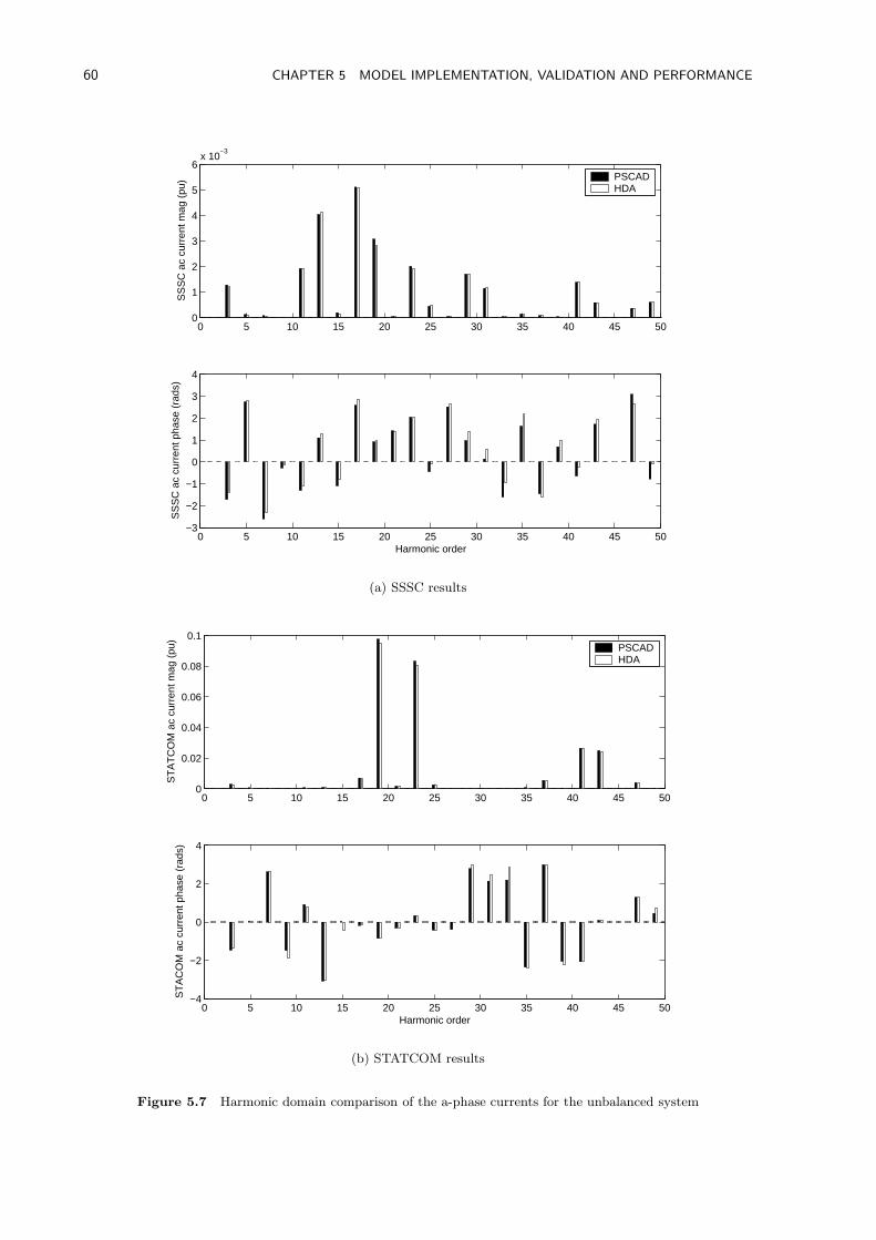
60 CHAPTER 5 MODEL IMPLEMENTATION, VALIDATION AND PERFORMANCE
0 5 10 15 20 25 30 35 40 45 500
1
2
3
4
5
6x 10
−3
SS
SC
ac
curr
ent m
ag (
pu)
0 5 10 15 20 25 30 35 40 45 50−3
−2
−1
0
1
2
3
4
Harmonic order
SS
SC
ac
curr
ent p
hase
(ra
ds)
PSCADHDA
(a) SSSC results
0 5 10 15 20 25 30 35 40 45 500
0.02
0.04
0.06
0.08
0.1
ST
AT
CO
M a
c cu
rren
t mag
(pu
)
0 5 10 15 20 25 30 35 40 45 50−4
−2
0
2
4
Harmonic order
ST
AC
OM
ac
curr
ent p
hase
(ra
ds)
PSCADHDA
(b) STATCOM results
Figure 5.7 Harmonic domain comparison of the a-phase currents for the unbalanced system
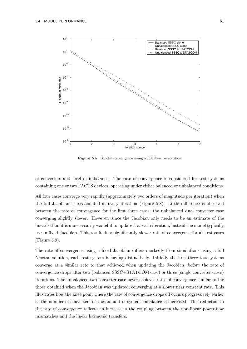
5.4 MODEL PERFORMANCE 61
1 2 3 4 5 6 710
−14
10−12
10−10
10−8
10−6
10−4
10−2
100
102
Iteration number
1−no
rm o
f mis
mat
ch
Balanced SSSC aloneUnbalanced SSSC aloneBalanced SSSC & STATCOMUnbalanced SSSC & STATCOM
Figure 5.8 Model convergence using a full Newton solution
of converters and level of imbalance. The rate of convergence is considered for test systems
containing one or two FACTS devices, operating under either balanced or unbalanced conditions.
All four cases converge very rapidly (approximately two orders of magnitude per iteration) when
the full Jacobian is recalculated at every iteration (Figure 5.8). Little difference is observed
between the rate of convergence for the first three cases, the unbalanced dual converter case
converging slightly slower. However, since the Jacobian only needs to be an estimate of the
linearisation it is unnecessarily wasteful to update it at each iteration, instead the model typically
uses a fixed Jacobian. This results in a significantly slower rate of convergence for all test cases
(Figure 5.9).
The rate of convergence using a fixed Jacobian differs markedly from simulations using a full
Newton solution, each test system behaving distinctively. Initially the first three test systems
converge at a similar rate to that achieved when updating the Jacobian, before the rate of
convergence drops after two (balanced SSSC+STATCOM case) or three (single converter cases)
iterations. The unbalanced two converter case never achieves rates of convergence similar to the
those obtained when the Jacobian was updated, converging at a slower near constant rate. This
illustrates how the knee point where the rate of convergence drops off occurs progressively earlier
as the number of converters or the amount of system imbalance is increased. This reduction in
the rate of convergence reflects an increase in the coupling between the non-linear power-flow
mismatches and the linear harmonic transfers.
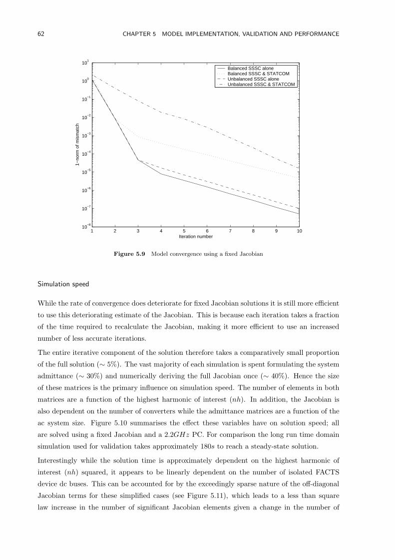
62 CHAPTER 5 MODEL IMPLEMENTATION, VALIDATION AND PERFORMANCE
1 2 3 4 5 6 7 8 9 1010
−8
10−7
10−6
10−5
10−4
10−3
10−2
10−1
100
101
Iteration number
1−no
rm o
f mis
mat
ch
Balanced SSSC aloneBalanced SSSC & STATCOMUnbalanced SSSC aloneUnbalanced SSSC & STATCOM
Figure 5.9 Model convergence using a fixed Jacobian
Simulation speed
While the rate of convergence does deteriorate for fixed Jacobian solutions it is still more efficient
to use this deteriorating estimate of the Jacobian. This is because each iteration takes a fraction
of the time required to recalculate the Jacobian, making it more efficient to use an increased
number of less accurate iterations.
The entire iterative component of the solution therefore takes a comparatively small proportion
of the full solution (∼ 5%). The vast majority of each simulation is spent formulating the system
admittance (∼ 30%) and numerically deriving the full Jacobian once (∼ 40%). Hence the size
of these matrices is the primary influence on simulation speed. The number of elements in both
matrices are a function of the highest harmonic of interest (nh). In addition, the Jacobian is
also dependent on the number of converters while the admittance matrices are a function of the
ac system size. Figure 5.10 summarises the effect these variables have on solution speed; all
are solved using a fixed Jacobian and a 2.2GHz PC. For comparison the long run time domain
simulation used for validation takes approximately 180s to reach a steady-state solution.
Interestingly while the solution time is approximately dependent on the highest harmonic of
interest (nh) squared, it appears to be linearly dependent on the number of isolated FACTS
device dc buses. This can be accounted for by the exceedingly sparse nature of the off-diagonal
Jacobian terms for these simplified cases (see Figure 5.11), which leads to a less than square
law increase in the number of significant Jacobian elements given a change in the number of
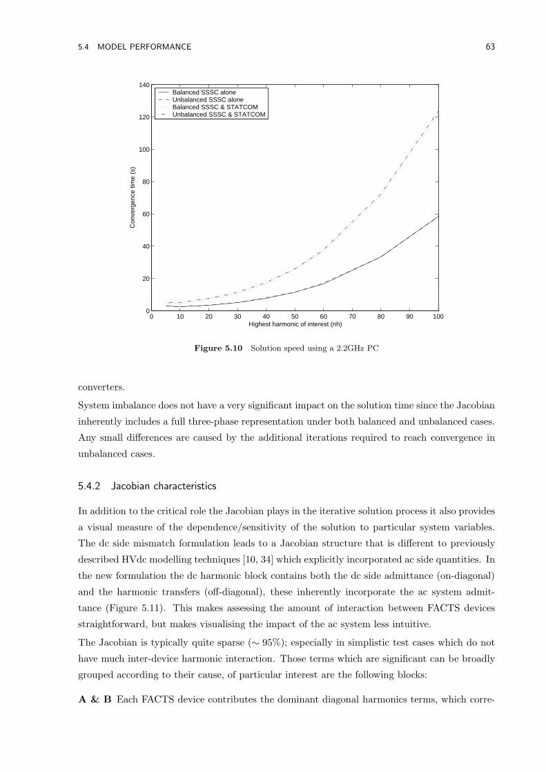
5.4 MODEL PERFORMANCE 63
0 10 20 30 40 50 60 70 80 90 1000
20
40
60
80
100
120
140
Highest harmonic of interest (nh)
Con
verg
ence
tim
e (s
)
Balanced SSSC aloneUnbalanced SSSC aloneBalanced SSSC & STATCOMUnbalanced SSSC & STATCOM
Figure 5.10 Solution speed using a 2.2GHz PC
converters.
System imbalance does not have a very significant impact on the solution time since the Jacobian
inherently includes a full three-phase representation under both balanced and unbalanced cases.
Any small differences are caused by the additional iterations required to reach convergence in
unbalanced cases.
5.4.2 Jacobian characteristics
In addition to the critical role the Jacobian plays in the iterative solution process it also provides
a visual measure of the dependence/sensitivity of the solution to particular system variables.
The dc side mismatch formulation leads to a Jacobian structure that is different to previously
described HVdc modelling techniques [10, 34] which explicitly incorporated ac side quantities. In
the new formulation the dc harmonic block contains both the dc side admittance (on-diagonal)
and the harmonic transfers (off-diagonal), these inherently incorporate the ac system admit-
tance (Figure 5.11). This makes assessing the amount of interaction between FACTS devices
straightforward, but makes visualising the impact of the ac system less intuitive.
The Jacobian is typically quite sparse (∼ 95%); especially in simplistic test cases which do not
have much inter-device harmonic interaction. Those terms which are significant can be broadly
grouped according to their cause, of particular interest are the following blocks:
A & B Each FACTS device contributes the dominant diagonal harmonics terms, which corre-
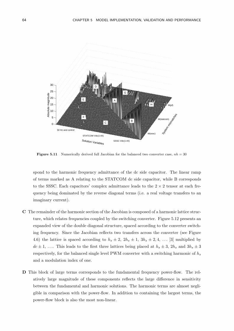
64 CHAPTER 5 MODEL IMPLEMENTATION, VALIDATION AND PERFORMANCE
0
5
10
15
20
25
30
Abs
olut
e m
agni
tude
E
C B
A
F
D
G
H
STATCOM Vdc(1:nh)
SSSC Vdc(1:nh)
50 Hz and control
Solution Variables
M(sssc) Syst
em m
ism
atch
es
M(statcom)
M(pf)
Figure 5.11 Numerically derived full Jacobian for the balanced two converter case, nh = 30
spond to the harmonic frequency admittance of the dc side capacitor. The linear ramp
of terms marked as A relating to the STATCOM dc side capacitor, while B corresponds
to the SSSC. Each capacitors’ complex admittance leads to the 2 × 2 tensor at each fre-
quency being dominated by the reverse diagonal terms (i.e. a real voltage transfers to an
imaginary current).
C The remainder of the harmonic section of the Jacobian is composed of a harmonic lattice struc-
ture, which relates frequencies coupled by the switching converter. Figure 5.12 presents an
expanded view of the double diagonal structure, spaced according to the converter switch-
ing frequency. Since the Jacobian reflects two transfers across the converter (see Figure
4.6) the lattice is spaced according to hs ± 2, 2hs ± 1, 3hs ± 2, 4, . . . [3] multiplied by
dc ± 1, . . .. This leads to the first three lattices being placed at hs ± 3, 2hs and 3hs ± 3
respectively, for the balanced single level PWM converter with a switching harmonic of hs
and a modulation index of one.
D This block of large terms corresponds to the fundamental frequency power-flow. The rel-
atively large magnitude of these components reflects the large difference in sensitivity
between the fundamental and harmonic solutions. The harmonic terms are almost negli-
gible in comparison with the power-flow. In addition to containing the largest terms, the
power-flow block is also the most non-linear.
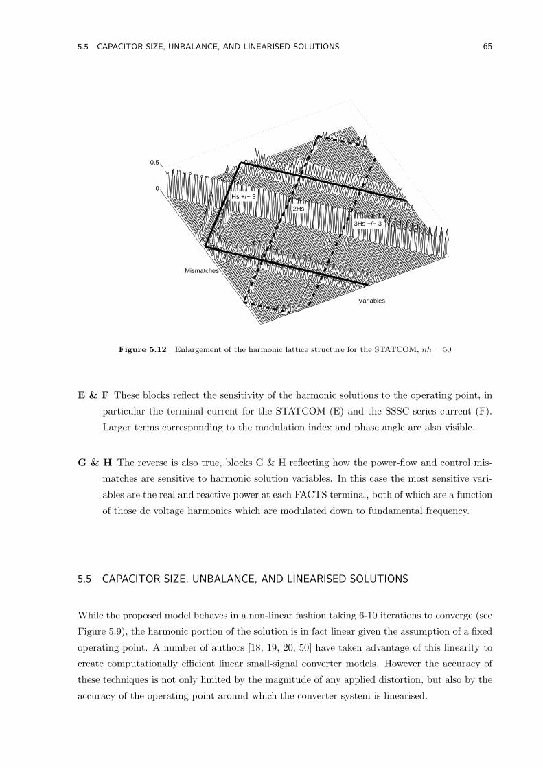
5.5 CAPACITOR SIZE, UNBALANCE, AND LINEARISED SOLUTIONS 65
0
0.5
Hs +/− 3
2Hs
3Hs +/− 3
Variables
Mismatches
Figure 5.12 Enlargement of the harmonic lattice structure for the STATCOM, nh = 50
E & F These blocks reflect the sensitivity of the harmonic solutions to the operating point, in
particular the terminal current for the STATCOM (E) and the SSSC series current (F).
Larger terms corresponding to the modulation index and phase angle are also visible.
G & H The reverse is also true, blocks G & H reflecting how the power-flow and control mis-
matches are sensitive to harmonic solution variables. In this case the most sensitive vari-
ables are the real and reactive power at each FACTS terminal, both of which are a function
of those dc voltage harmonics which are modulated down to fundamental frequency.
5.5 CAPACITOR SIZE, UNBALANCE, AND LINEARISED SOLUTIONS
While the proposed model behaves in a non-linear fashion taking 6-10 iterations to converge (see
Figure 5.9), the harmonic portion of the solution is in fact linear given the assumption of a fixed
operating point. A number of authors [18, 19, 20, 50] have taken advantage of this linearity to
create computationally efficient linear small-signal converter models. However the accuracy of
these techniques is not only limited by the magnitude of any applied distortion, but also by the
accuracy of the operating point around which the converter system is linearised.
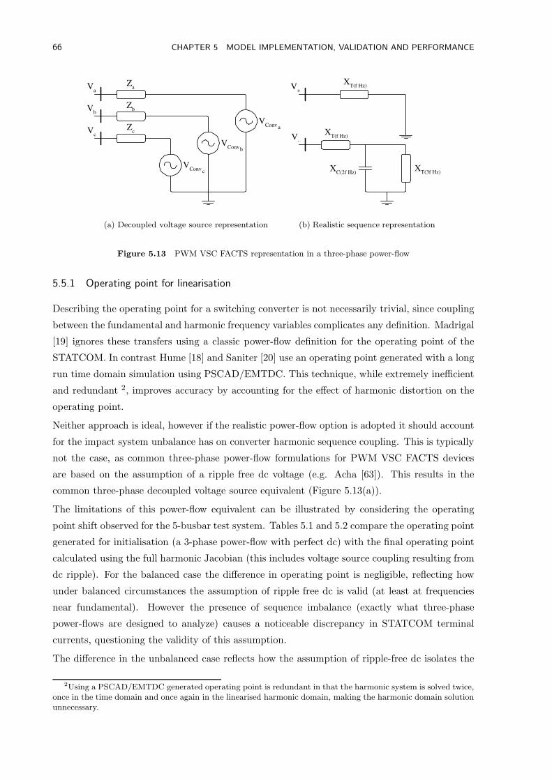
66 CHAPTER 5 MODEL IMPLEMENTATION, VALIDATION AND PERFORMANCE
V a
V b
V c
Z a
Z b
Z c
V Conv
V Conv
V Conv
a
b
c
(a) Decoupled voltage source representation
V +
V -
X T(f Hz)
X T(f Hz)
X C(2f Hz)
X T(3f Hz)
(b) Realistic sequence representation
Figure 5.13 PWM VSC FACTS representation in a three-phase power-flow
5.5.1 Operating point for linearisation
Describing the operating point for a switching converter is not necessarily trivial, since coupling
between the fundamental and harmonic frequency variables complicates any definition. Madrigal
[19] ignores these transfers using a classic power-flow definition for the operating point of the
STATCOM. In contrast Hume [18] and Saniter [20] use an operating point generated with a long
run time domain simulation using PSCAD/EMTDC. This technique, while extremely inefficient
and redundant 2, improves accuracy by accounting for the effect of harmonic distortion on the
operating point.
Neither approach is ideal, however if the realistic power-flow option is adopted it should account
for the impact system unbalance has on converter harmonic sequence coupling. This is typically
not the case, as common three-phase power-flow formulations for PWM VSC FACTS devices
are based on the assumption of a ripple free dc voltage (e.g. Acha [63]). This results in the
common three-phase decoupled voltage source equivalent (Figure 5.13(a)).
The limitations of this power-flow equivalent can be illustrated by considering the operating
point shift observed for the 5-busbar test system. Tables 5.1 and 5.2 compare the operating point
generated for initialisation (a 3-phase power-flow with perfect dc) with the final operating point
calculated using the full harmonic Jacobian (this includes voltage source coupling resulting from
dc ripple). For the balanced case the difference in operating point is negligible, reflecting how
under balanced circumstances the assumption of ripple free dc is valid (at least at frequencies
near fundamental). However the presence of sequence imbalance (exactly what three-phase
power-flows are designed to analyze) causes a noticeable discrepancy in STATCOM terminal
currents, questioning the validity of this assumption.
The difference in the unbalanced case reflects how the assumption of ripple-free dc isolates the
2Using a PSCAD/EMTDC generated operating point is redundant in that the harmonic system is solved twice,once in the time domain and once again in the linearised harmonic domain, making the harmonic domain solutionunnecessary.
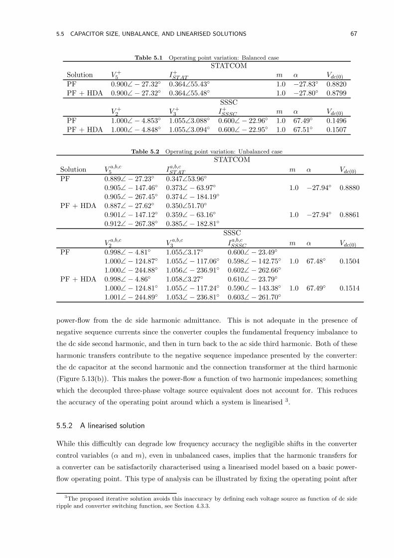
5.5 CAPACITOR SIZE, UNBALANCE, AND LINEARISED SOLUTIONS 67
Table 5.1 Operating point variation: Balanced case
STATCOMSolution V +
5 I+STAT m α Vdc(0)
PF 0.900∠ − 27.32 0.364∠55.43 1.0 −27.83 0.8820PF + HDA 0.900∠ − 27.32 0.364∠55.48 1.0 −27.80 0.8799
SSSCV +
2 V +3 I+
SSSC m α Vdc(0)PF 1.000∠ − 4.853 1.055∠3.088 0.600∠ − 22.96 1.0 67.49 0.1496PF + HDA 1.000∠ − 4.848 1.055∠3.094 0.600∠ − 22.95 1.0 67.51 0.1507
Table 5.2 Operating point variation: Unbalanced case
STATCOM
Solution V a,b,c5 Ia,b,cSTAT m α Vdc(0)
PF 0.889∠ − 27.23 0.347∠53.96
0.905∠ − 147.46 0.373∠ − 63.97 1.0 −27.94 0.88800.905∠ − 267.45 0.374∠ − 184.19
PF + HDA 0.887∠ − 27.62 0.350∠51.70
0.901∠ − 147.12 0.359∠ − 63.16 1.0 −27.94 0.88610.912∠ − 267.38 0.385∠ − 182.81
SSSC
V a,b,c2 V a,b,c
3 Ia,b,cSSSC m α Vdc(0)PF 0.998∠ − 4.81 1.055∠3.17 0.600∠ − 23.49
1.000∠ − 124.87 1.055∠ − 117.06 0.598∠ − 142.75 1.0 67.48 0.15041.000∠ − 244.88 1.056∠ − 236.91 0.602∠ − 262.66
PF + HDA 0.998∠ − 4.86 1.058∠3.27 0.610∠ − 23.79
1.000∠ − 124.81 1.055∠ − 117.24 0.590∠ − 143.38 1.0 67.49 0.15141.001∠ − 244.89 1.053∠ − 236.81 0.603∠ − 261.70
power-flow from the dc side harmonic admittance. This is not adequate in the presence of
negative sequence currents since the converter couples the fundamental frequency imbalance to
the dc side second harmonic, and then in turn back to the ac side third harmonic. Both of these
harmonic transfers contribute to the negative sequence impedance presented by the converter:
the dc capacitor at the second harmonic and the connection transformer at the third harmonic
(Figure 5.13(b)). This makes the power-flow a function of two harmonic impedances; something
which the decoupled three-phase voltage source equivalent does not account for. This reduces
the accuracy of the operating point around which a system is linearised 3.
5.5.2 A linearised solution
While this difficultly can degrade low frequency accuracy the negligible shifts in the converter
control variables (α and m), even in unbalanced cases, implies that the harmonic transfers for
a converter can be satisfactorily characterised using a linearised model based on a basic power-
flow operating point. This type of analysis can be illustrated by fixing the operating point after
3The proposed iterative solution avoids this inaccuracy by defining each voltage source as function of dc sideripple and converter switching function, see Section 4.3.3.
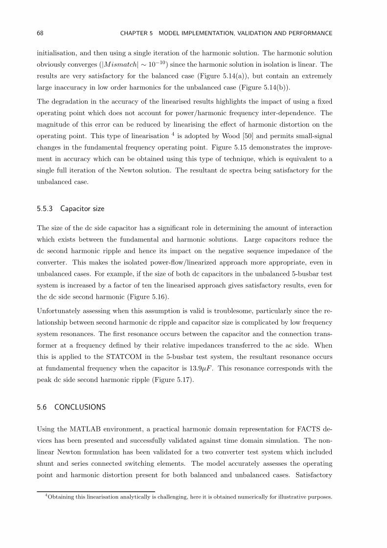
68 CHAPTER 5 MODEL IMPLEMENTATION, VALIDATION AND PERFORMANCE
initialisation, and then using a single iteration of the harmonic solution. The harmonic solution
obviously converges (|Mismatch| ∼ 10−10) since the harmonic solution in isolation is linear. The
results are very satisfactory for the balanced case (Figure 5.14(a)), but contain an extremely
large inaccuracy in low order harmonics for the unbalanced case (Figure 5.14(b)).
The degradation in the accuracy of the linearised results highlights the impact of using a fixed
operating point which does not account for power/harmonic frequency inter-dependence. The
magnitude of this error can be reduced by linearising the effect of harmonic distortion on the
operating point. This type of linearisation 4 is adopted by Wood [50] and permits small-signal
changes in the fundamental frequency operating point. Figure 5.15 demonstrates the improve-
ment in accuracy which can be obtained using this type of technique, which is equivalent to a
single full iteration of the Newton solution. The resultant dc spectra being satisfactory for the
unbalanced case.
5.5.3 Capacitor size
The size of the dc side capacitor has a significant role in determining the amount of interaction
which exists between the fundamental and harmonic solutions. Large capacitors reduce the
dc second harmonic ripple and hence its impact on the negative sequence impedance of the
converter. This makes the isolated power-flow/linearized approach more appropriate, even in
unbalanced cases. For example, if the size of both dc capacitors in the unbalanced 5-busbar test
system is increased by a factor of ten the linearised approach gives satisfactory results, even for
the dc side second harmonic (Figure 5.16).
Unfortunately assessing when this assumption is valid is troublesome, particularly since the re-
lationship between second harmonic dc ripple and capacitor size is complicated by low frequency
system resonances. The first resonance occurs between the capacitor and the connection trans-
former at a frequency defined by their relative impedances transferred to the ac side. When
this is applied to the STATCOM in the 5-busbar test system, the resultant resonance occurs
at fundamental frequency when the capacitor is 13.9µF . This resonance corresponds with the
peak dc side second harmonic ripple (Figure 5.17).
5.6 CONCLUSIONS
Using the MATLAB environment, a practical harmonic domain representation for FACTS de-
vices has been presented and successfully validated against time domain simulation. The non-
linear Newton formulation has been validated for a two converter test system which included
shunt and series connected switching elements. The model accurately assesses the operating
point and harmonic distortion present for both balanced and unbalanced cases. Satisfactory
4Obtaining this linearisation analytically is challenging, here it is obtained numerically for illustrative purposes.
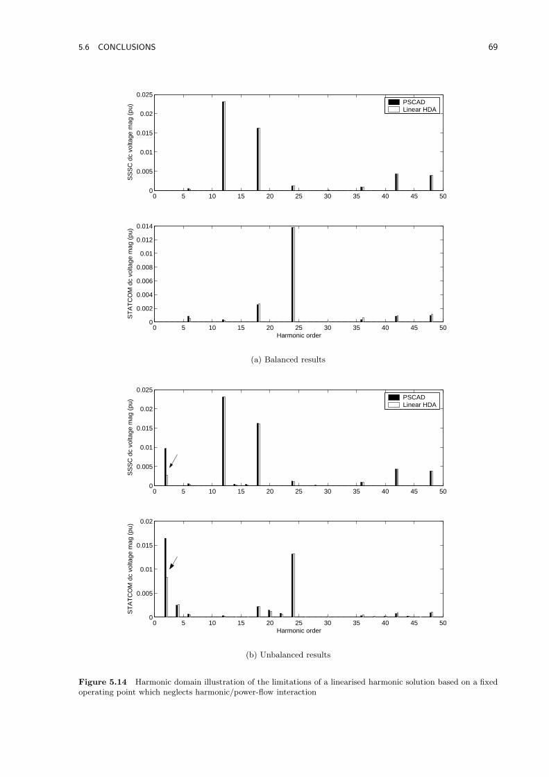
5.6 CONCLUSIONS 69
0 5 10 15 20 25 30 35 40 45 500
0.005
0.01
0.015
0.02
0.025
SS
SC
dc
volta
ge m
ag (
pu)
0 5 10 15 20 25 30 35 40 45 500
0.002
0.004
0.006
0.008
0.01
0.012
0.014
Harmonic order
ST
AT
CO
M d
c vo
ltage
mag
(pu
)
PSCADLinear HDA
(a) Balanced results
0 5 10 15 20 25 30 35 40 45 500
0.005
0.01
0.015
0.02
0.025
SS
SC
dc
volta
ge m
ag (
pu)
0 5 10 15 20 25 30 35 40 45 500
0.005
0.01
0.015
0.02
Harmonic order
ST
AT
CO
M d
c vo
ltage
mag
(pu
)
PSCADLinear HDA
(b) Unbalanced results
Figure 5.14 Harmonic domain illustration of the limitations of a linearised harmonic solution based on a fixedoperating point which neglects harmonic/power-flow interaction
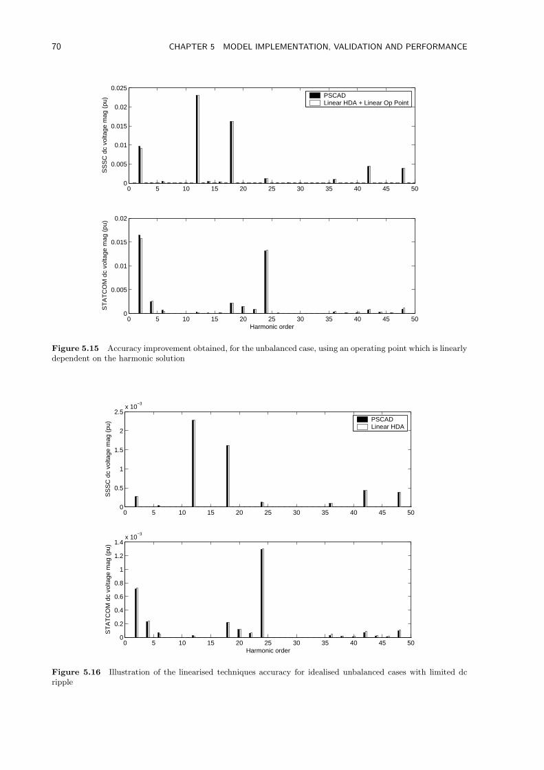
70 CHAPTER 5 MODEL IMPLEMENTATION, VALIDATION AND PERFORMANCE
0 5 10 15 20 25 30 35 40 45 500
0.005
0.01
0.015
0.02
0.025
SS
SC
dc
volta
ge m
ag (
pu)
0 5 10 15 20 25 30 35 40 45 500
0.005
0.01
0.015
0.02
Harmonic order
ST
AT
CO
M d
c vo
ltage
mag
(pu
)PSCADLinear HDA + Linear Op Point
Figure 5.15 Accuracy improvement obtained, for the unbalanced case, using an operating point which is linearlydependent on the harmonic solution
0 5 10 15 20 25 30 35 40 45 500
0.5
1
1.5
2
2.5x 10
−3
SS
SC
dc
volta
ge m
ag (
pu)
0 5 10 15 20 25 30 35 40 45 500
0.2
0.4
0.6
0.8
1
1.2
1.4x 10
−3
Harmonic order
ST
AT
CO
M d
c vo
ltage
mag
(pu
)
PSCADLinear HDA
Figure 5.16 Illustration of the linearised techniques accuracy for idealised unbalanced cases with limited dcripple
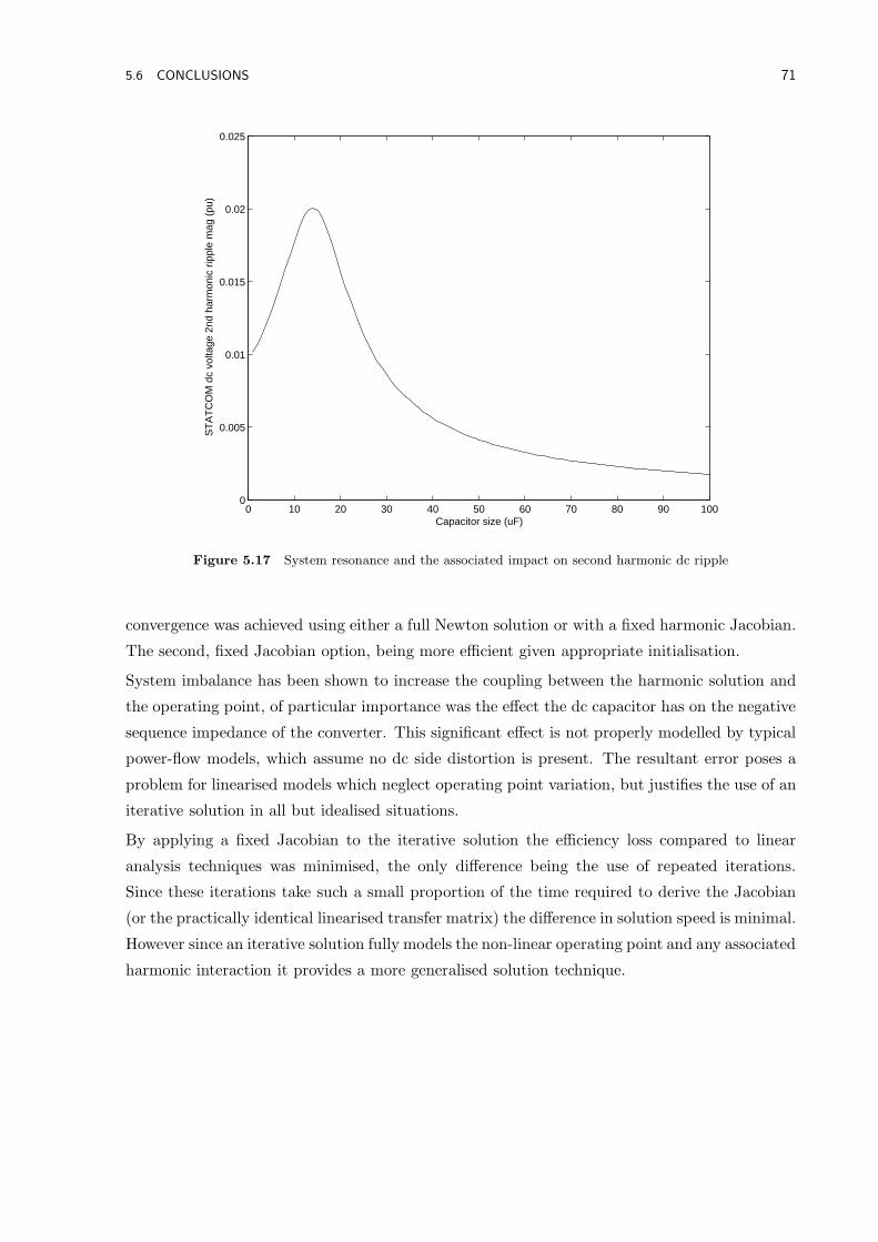
5.6 CONCLUSIONS 71
0 10 20 30 40 50 60 70 80 90 1000
0.005
0.01
0.015
0.02
0.025
Capacitor size (uF)
ST
AT
CO
M d
c vo
ltage
2nd
har
mon
ic r
ippl
e m
ag (
pu)
Figure 5.17 System resonance and the associated impact on second harmonic dc ripple
convergence was achieved using either a full Newton solution or with a fixed harmonic Jacobian.
The second, fixed Jacobian option, being more efficient given appropriate initialisation.
System imbalance has been shown to increase the coupling between the harmonic solution and
the operating point, of particular importance was the effect the dc capacitor has on the negative
sequence impedance of the converter. This significant effect is not properly modelled by typical
power-flow models, which assume no dc side distortion is present. The resultant error poses a
problem for linearised models which neglect operating point variation, but justifies the use of an
iterative solution in all but idealised situations.
By applying a fixed Jacobian to the iterative solution the efficiency loss compared to linear
analysis techniques was minimised, the only difference being the use of repeated iterations.
Since these iterations take such a small proportion of the time required to derive the Jacobian
(or the practically identical linearised transfer matrix) the difference in solution speed is minimal.
However since an iterative solution fully models the non-linear operating point and any associated
harmonic interaction it provides a more generalised solution technique.

Chapter 6
FACTS DEVICE INTERACTION
6.1 INTRODUCTION
As converter systems become increasingly prevalent in power systems worldwide, the nature
and impact of harmonic interaction between FACTS devices becomes increasingly important.
Assessing this interaction has two critical components: first calculating the aggregate effect
of multiple converters, and second quantifying the contribution of each converter. The first
objective is primarily a computational problem, a compromise between system scale and solution
speed, the second poses a more challenging problem.
Separating the contribution each converter makes to the aggregate distortion is complicated by
each converter’s dependence on the terminal conditions to which it is connected. This makes
it difficult, if not impossible, to assign any particular harmonic to a single converter. Since
the harmonic domain explicitly models this harmonic interdependence it offers a significant
advantage over equivalent time domain methods for this type of analysis. This Chapter uses this
advantage, in particular the solution Jacobian, to consider the ac and dc side interdependence
of systems containing two PWM converters.
6.2 AC SIDE INTERACTION
The first aspect of FACTS device interaction considered is the amount of ac side interaction
which occurs between individual FACTS devices. This is critical since accurately modelling the
entirety of an ac power system is often not feasible, making it necessary to reduce the system
beyond some boundary to an equivalent circuit. Determining where to place this boundary is
dependent on the nature of the converters and interconnecting ac system. This Section considers
three ac cases with varying amount of ac side interaction, outlining some determinants of ac side
interaction.
6.2.1 Dominant low-pass interconnection
Simplistic test systems, like that used in Chapter 5 and innumerable papers, typically behave ac-
cording to a low-pass characteristic. This is a result of fixed series impedances used to represent
74 CHAPTER 6 FACTS DEVICE INTERACTION
transmission systems. The resultant attenuation at higher harmonic frequencies limits converter
interdependence almost entirely to fundamental frequency, this is reflected in the system Jaco-
bian which contains practically no off-diagonal block components (Figure 6.1(a)). As such the
accuracy of the harmonic assessment for this case is not markedly affected by the assumption
of converter independence at harmonic frequencies. This can be illustrated by setting the off-
diagonal Jacobian blocks to zero, the resultant dc terminal voltages being practically identical
(Figure 6.1(b)).
The similarity observed in the results reflects the near independent nature of the solution vari-
ables for each converter (Vdc1:nh), as distinct from the lack of any interaction between the devices.
In fact when the ac terminal current spectra are calculated (post-convergence) significant dif-
ferences exist between the approximate harmonic domain solution and the full time domain
representation (see Figure 6.2). The comparative independence of the dc side voltages is a
function of two important mechanisms: the frequency and phase dependent impedance of each
converter, and the low-pass ac system characteristic. In this case, the combination of these two
effects isolates the solution variables (Vdc) somewhat unrealistically. Including a transmission
line model increases the ac system sensitivity at some harmonic frequencies (due to resonances),
thereby reducing this isolation.
6.2.2 Realistic transmission systems
In contrast to the idealised systems typically used to validate harmonic domain analysis tech-
niques, actual transmission systems do not conform to a low-pass characteristic. Conductor ge-
ometry and the length of transmission lines leads to phase imbalance and harmonic resonances.
Both these affect the harmonics generated by a convertor: imbalance causes the generation of
non-characteristic harmonics, while the resonances lead to reduced interconnecting impedances.
These transmission line characteristics are incorporated using a three-phase equivalent-pi, ini-
tially derived from the model included in PSCAD/EMTDC. Then, after validation, the sensitiv-
ity of harmonic solution to small transmission line variations is illustrated by comparing these
results with an analytic model based on line images and Carson’s corrections for earth return
(outlined in Appendix C).
Model validation with transmission system resonances
Including these phenomena has a dramatic effect on both the system Jacobian and the resultant
electrical quantities. The transmission lines shunt capacitance (not modelled for the low-pass
case) leads to a small shift in the fundamental frequency operating point, and a number of
complex harmonic resonances. These resonances increase the solution’s sensitivity to particu-
lar frequencies, contributing a large number of additional off-diagonal terms to the harmonic
Jacobian (see Figure 6.3(a)). The increase in ac system complexity does not have a noticeable
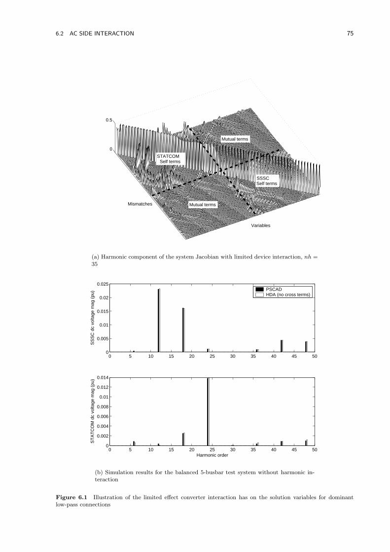
6.2 AC SIDE INTERACTION 75
0
0.5
Variables
Mismatches
STATCOM Self terms
SSSC Self terms
Mutual terms
Mutual terms
(a) Harmonic component of the system Jacobian with limited device interaction, nh =35
0 5 10 15 20 25 30 35 40 45 500
0.005
0.01
0.015
0.02
0.025
SS
SC
dc
volta
ge m
ag (
pu)
0 5 10 15 20 25 30 35 40 45 500
0.002
0.004
0.006
0.008
0.01
0.012
0.014
Harmonic order
ST
AT
CO
M d
c vo
ltage
mag
(pu
)
PSCADHDA (no cross terms)
(b) Simulation results for the balanced 5-busbar test system without harmonic in-teraction
Figure 6.1 Illustration of the limited effect converter interaction has on the solution variables for dominantlow-pass connections
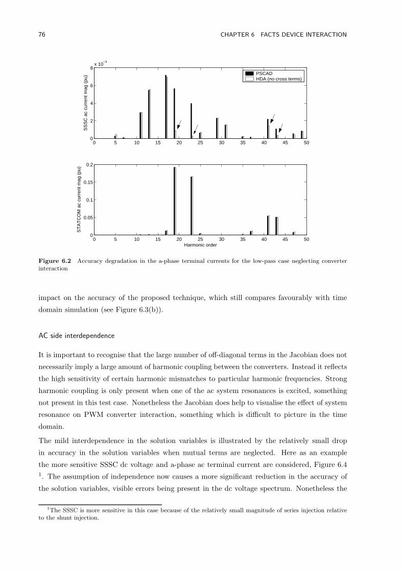
76 CHAPTER 6 FACTS DEVICE INTERACTION
0 5 10 15 20 25 30 35 40 45 500
2
4
6
8x 10
−3
SS
SC
ac
curr
ent m
ag (
pu)
0 5 10 15 20 25 30 35 40 45 500
0.05
0.1
0.15
0.2
Harmonic order
ST
AT
CO
M a
c cu
rren
t mag
(pu
)PSCADHDA (no cross terms)
Figure 6.2 Accuracy degradation in the a-phase terminal currents for the low-pass case neglecting converterinteraction
impact on the accuracy of the proposed technique, which still compares favourably with time
domain simulation (see Figure 6.3(b)).
AC side interdependence
It is important to recognise that the large number of off-diagonal terms in the Jacobian does not
necessarily imply a large amount of harmonic coupling between the converters. Instead it reflects
the high sensitivity of certain harmonic mismatches to particular harmonic frequencies. Strong
harmonic coupling is only present when one of the ac system resonances is excited, something
not present in this test case. Nonetheless the Jacobian does help to visualise the effect of system
resonance on PWM converter interaction, something which is difficult to picture in the time
domain.
The mild interdependence in the solution variables is illustrated by the relatively small drop
in accuracy in the solution variables when mutual terms are neglected. Here as an example
the more sensitive SSSC dc voltage and a-phase ac terminal current are considered, Figure 6.41. The assumption of independence now causes a more significant reduction in the accuracy of
the solution variables, visible errors being present in the dc voltage spectrum. Nonetheless the
1The SSSC is more sensitive in this case because of the relatively small magnitude of series injection relativeto the shunt injection.
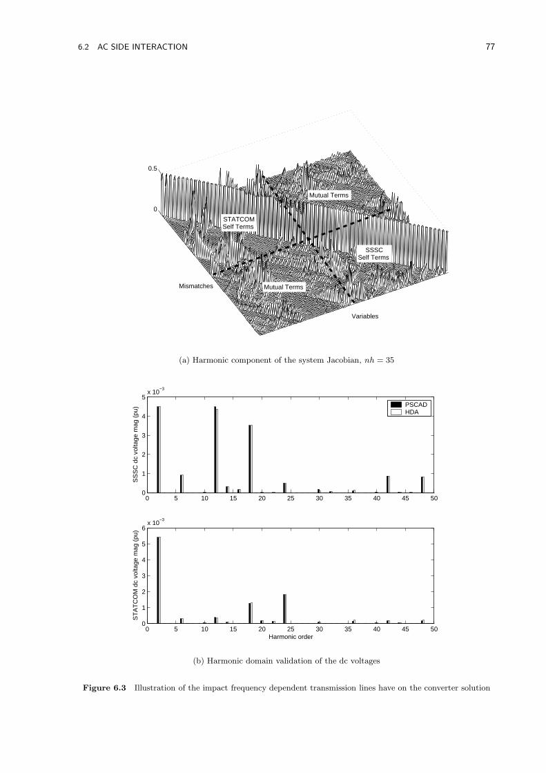
6.2 AC SIDE INTERACTION 77
0
0.5
Variables
Mismatches
STATCOMSelf Terms
SSSCSelf Terms
Mutual Terms
Mutual Terms
(a) Harmonic component of the system Jacobian, nh = 35
0 5 10 15 20 25 30 35 40 45 500
1
2
3
4
5x 10
−3
SS
SC
dc
volta
ge m
ag (
pu)
0 5 10 15 20 25 30 35 40 45 500
1
2
3
4
5
6x 10
−3
Harmonic order
ST
AT
CO
M d
c vo
ltage
mag
(pu
)
PSCADHDA
(b) Harmonic domain validation of the dc voltages
Figure 6.3 Illustration of the impact frequency dependent transmission lines have on the converter solution

78 CHAPTER 6 FACTS DEVICE INTERACTION
0 5 10 15 20 25 30 35 40 45 500
1
2
3
4
5x 10
−3
SS
SC
dc
volta
ge m
ag (
pu)
0 5 10 15 20 25 30 35 40 45 500
0.01
0.02
0.03
0.04
Harmonic order
SS
SC
ac
curr
ent m
ag (
pu)
PSCADHDA (no cross terms)
Figure 6.4 Illustration of the degraded solution accuracy for the SSSC when mutual coupling is neglected withtransmission systems present
dc spectrum is still dominated by the characteristic terms which remain relatively unaffected,
despite not modelling the mutual terms. Once again the similarity between the full and ap-
proximate solution is not observed in the ac side current spectra, which is clearly a function of
harmonic distortion introduced by the STATCOM.
The contrasting effect this approximation has on the ac and dc side electrical quantities reinforces
the blocking effect of the frequency and phase dependent impedance presented by a PWM
converter. While ac terminal distortion is linearly dependent on all other ac distorting signals
(i.e. no harmonic coupling), the dc side distortion is only a function of other distorting signals
when these signals coincide with elements of the converter’s PWM spectrum. As a result the
two dc side voltages in the test system are all but independent since few of the STATCOM and
SSSC PWM harmonics coincide. The only significant discrepancy occurs at the 6th dc harmonic.
Lowering the switching frequency of the STATCOM to match the SSSC shifts the Jacobian
peaks in the mutual blocks such that they align with the peaks in the self blocks, increasing
the interdependence of the solution variables. The comparative magnitude of the two injected
voltages leads to the STATCOM being relatively unaffected, while the smaller SSSC dc side
spectrum is heavily affected by the distortion introduced by the STATCOM (Figure 6.5). All of
the characteristic SSSC harmonics now show significant inaccuracy, the only exception is the 2nd
harmonic which is derived from the power-flow coupling which was still modelled. While this is
an extreme example, it does illustrate the difficultly associated with accurately partitioning a
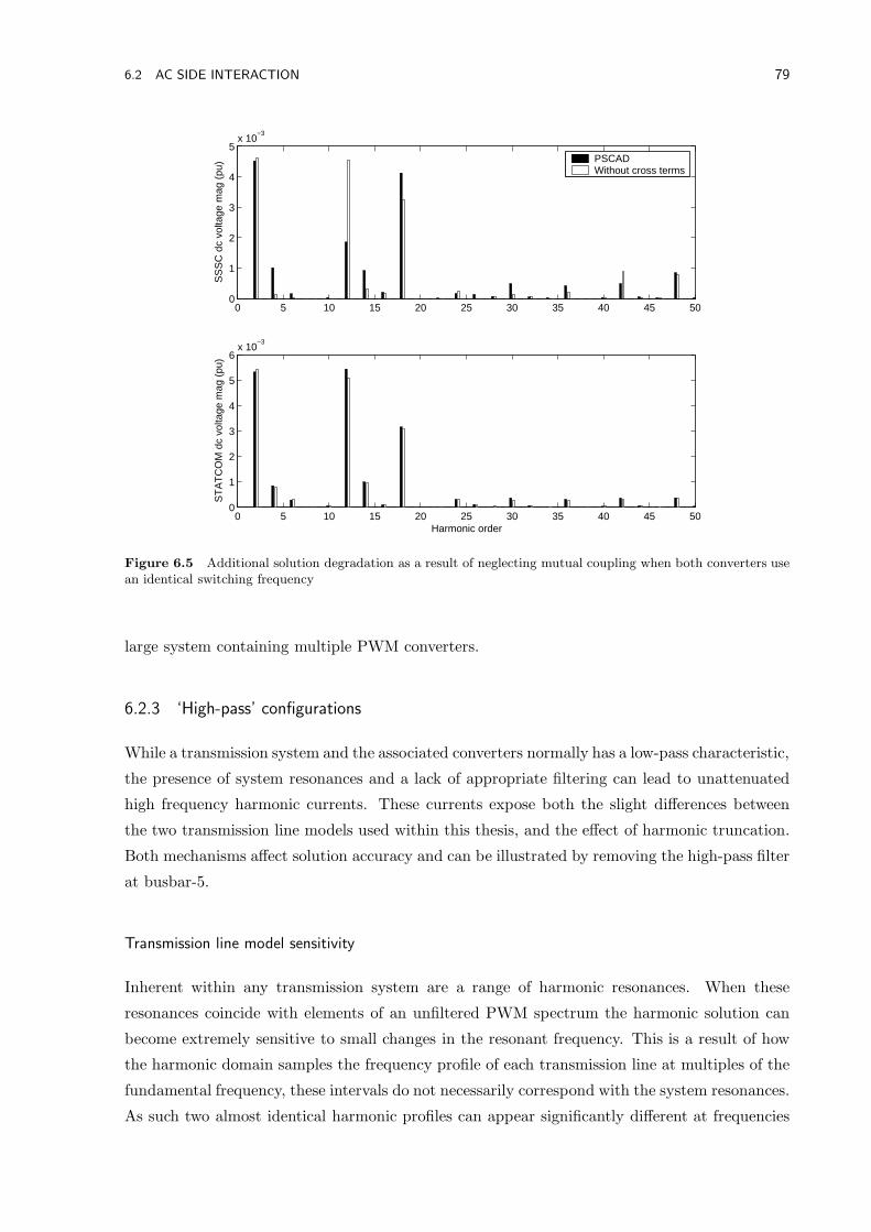
6.2 AC SIDE INTERACTION 79
0 5 10 15 20 25 30 35 40 45 500
1
2
3
4
5x 10
−3
SS
SC
dc
volta
ge m
ag (
pu)
0 5 10 15 20 25 30 35 40 45 500
1
2
3
4
5
6x 10
−3
Harmonic order
ST
AT
CO
M d
c vo
ltage
mag
(pu
)
PSCADWithout cross terms
Figure 6.5 Additional solution degradation as a result of neglecting mutual coupling when both converters usean identical switching frequency
large system containing multiple PWM converters.
6.2.3 ‘High-pass’ configurations
While a transmission system and the associated converters normally has a low-pass characteristic,
the presence of system resonances and a lack of appropriate filtering can lead to unattenuated
high frequency harmonic currents. These currents expose both the slight differences between
the two transmission line models used within this thesis, and the effect of harmonic truncation.
Both mechanisms affect solution accuracy and can be illustrated by removing the high-pass filter
at busbar-5.
Transmission line model sensitivity
Inherent within any transmission system are a range of harmonic resonances. When these
resonances coincide with elements of an unfiltered PWM spectrum the harmonic solution can
become extremely sensitive to small changes in the resonant frequency. This is a result of how
the harmonic domain samples the frequency profile of each transmission line at multiples of the
fundamental frequency, these intervals do not necessarily correspond with the system resonances.
As such two almost identical harmonic profiles can appear significantly different at frequencies
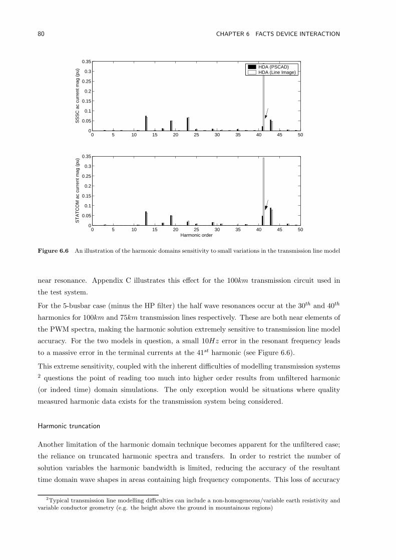
80 CHAPTER 6 FACTS DEVICE INTERACTION
0 5 10 15 20 25 30 35 40 45 500
0.05
0.1
0.15
0.2
0.25
0.3
0.35
SS
SC
ac
curr
ent m
ag (
pu)
0 5 10 15 20 25 30 35 40 45 500
0.05
0.1
0.15
0.2
0.25
0.3
0.35
Harmonic order
ST
AT
CO
M a
c cu
rren
t mag
(pu
)
HDA (PSCAD)HDA (Line Image)
Figure 6.6 An illustration of the harmonic domains sensitivity to small variations in the transmission line model
near resonance. Appendix C illustrates this effect for the 100km transmission circuit used in
the test system.
For the 5-busbar case (minus the HP filter) the half wave resonances occur at the 30th and 40th
harmonics for 100km and 75km transmission lines respectively. These are both near elements of
the PWM spectra, making the harmonic solution extremely sensitive to transmission line model
accuracy. For the two models in question, a small 10Hz error in the resonant frequency leads
to a massive error in the terminal currents at the 41st harmonic (see Figure 6.6).
This extreme sensitivity, coupled with the inherent difficulties of modelling transmission systems
2 questions the point of reading too much into higher order results from unfiltered harmonic
(or indeed time) domain simulations. The only exception would be situations where quality
measured harmonic data exists for the transmission system being considered.
Harmonic truncation
Another limitation of the harmonic domain technique becomes apparent for the unfiltered case;
the reliance on truncated harmonic spectra and transfers. In order to restrict the number of
solution variables the harmonic bandwidth is limited, reducing the accuracy of the resultant
time domain wave shapes in areas containing high frequency components. This loss of accuracy
2Typical transmission line modelling difficulties can include a non-homogeneous/variable earth resistivity andvariable conductor geometry (e.g. the height above the ground in mountainous regions)
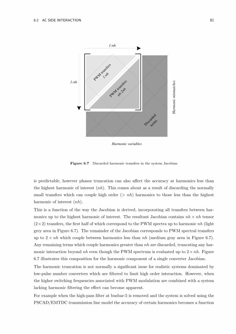
6.2 AC SIDE INTERACTION 81
1:nh
1:nh PW
M tr
ansf
ers
1:nh
PWM
tran
sfer
s
nh:2
nh
Disca
rded
term
s
Harmonic variables
Ha
rmo
nic
mis
ma
tch
es
Figure 6.7 Discarded harmonic transfers in the system Jacobian
is predictable, however phasor truncation can also affect the accuracy at harmonics less than
the highest harmonic of interest (nh). This comes about as a result of discarding the normally
small transfers which can couple high order (> nh) harmonics to those less than the highest
harmonic of interest (nh).
This is a function of the way the Jacobian is derived, incorporating all transfers between har-
monics up to the highest harmonic of interest. The resultant Jacobian contains nh× nh tensor
(2×2) transfers, the first half of which correspond to the PWM spectra up to harmonic nh (light
grey area in Figure 6.7). The remainder of the Jacobian corresponds to PWM spectral transfers
up to 2 × nh which couple between harmonics less than nh (medium gray area in Figure 6.7).
Any remaining terms which couple harmonics greater than nh are discarded, truncating any har-
monic interaction beyond nh even though the PWM spectrum is evaluated up to 2×nh. Figure
6.7 illustrates this composition for the harmonic component of a single converter Jacobian.
The harmonic truncation is not normally a significant issue for realistic systems dominated by
low-pulse number converters which are filtered to limit high order interaction. However, when
the higher switching frequencies associated with PWM modulation are combined with a system
lacking harmonic filtering the effect can become apparent.
For example when the high-pass filter at busbar-5 is removed and the system is solved using the
PSCAD/EMTDC transmission line model the accuracy of certain harmonics becomes a function
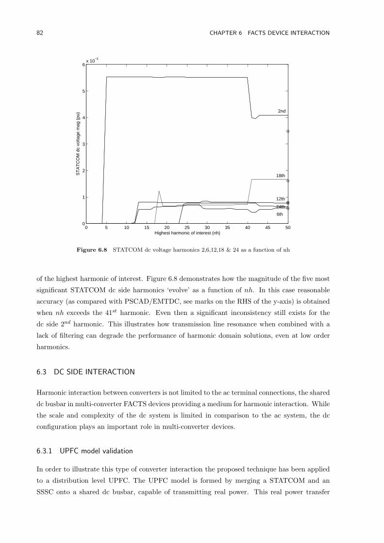
82 CHAPTER 6 FACTS DEVICE INTERACTION
0 5 10 15 20 25 30 35 40 45 500
1
2
3
4
5
6x 10
−3
Highest harmonic of interest (nh)
ST
AT
CO
M d
c vo
ltage
mag
(pu
) 2nd
18th
12th
6th
24th
Figure 6.8 STATCOM dc voltage harmonics 2,6,12,18 & 24 as a function of nh
of the highest harmonic of interest. Figure 6.8 demonstrates how the magnitude of the five most
significant STATCOM dc side harmonics ‘evolve’ as a function of nh. In this case reasonable
accuracy (as compared with PSCAD/EMTDC, see marks on the RHS of the y-axis) is obtained
when nh exceeds the 41st harmonic. Even then a significant inconsistency still exists for the
dc side 2nd harmonic. This illustrates how transmission line resonance when combined with a
lack of filtering can degrade the performance of harmonic domain solutions, even at low order
harmonics.
6.3 DC SIDE INTERACTION
Harmonic interaction between converters is not limited to the ac terminal connections, the shared
dc busbar in multi-converter FACTS devices providing a medium for harmonic interaction. While
the scale and complexity of the dc system is limited in comparison to the ac system, the dc
configuration plays an important role in multi-converter devices.
6.3.1 UPFC model validation
In order to illustrate this type of converter interaction the proposed technique has been applied
to a distribution level UPFC. The UPFC model is formed by merging a STATCOM and an
SSSC onto a shared dc busbar, capable of transmitting real power. This real power transfer
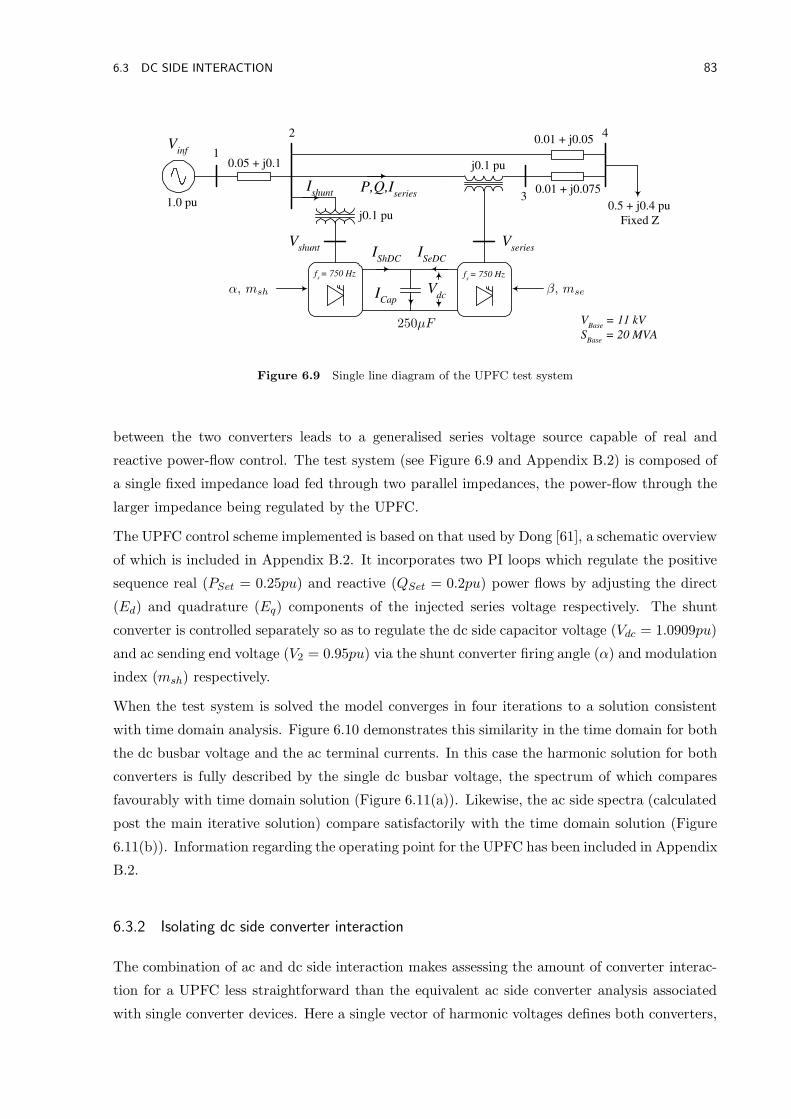
6.3 DC SIDE INTERACTION 83
V series
P,Q,I series
V dc
I ShDC
I SeDC
I Cap
V shunt
I shunt
V inf
0.05 + j0.1
0.01 + j0.05
0.01 + j0.075
0.5 + j0.4 pu
Fixed Z j0.1 pu
j0.1 pu 1
f s = 750 Hz f
s = 750 Hz
1.0 pu
V Base
= 11 kV
S Base
= 20 MVA
2
3
4
α, msh β, mse
250µF
Figure 6.9 Single line diagram of the UPFC test system
between the two converters leads to a generalised series voltage source capable of real and
reactive power-flow control. The test system (see Figure 6.9 and Appendix B.2) is composed of
a single fixed impedance load fed through two parallel impedances, the power-flow through the
larger impedance being regulated by the UPFC.
The UPFC control scheme implemented is based on that used by Dong [61], a schematic overview
of which is included in Appendix B.2. It incorporates two PI loops which regulate the positive
sequence real (PSet = 0.25pu) and reactive (QSet = 0.2pu) power flows by adjusting the direct
(Ed) and quadrature (Eq) components of the injected series voltage respectively. The shunt
converter is controlled separately so as to regulate the dc side capacitor voltage (Vdc = 1.0909pu)
and ac sending end voltage (V2 = 0.95pu) via the shunt converter firing angle (α) and modulation
index (msh) respectively.
When the test system is solved the model converges in four iterations to a solution consistent
with time domain analysis. Figure 6.10 demonstrates this similarity in the time domain for both
the dc busbar voltage and the ac terminal currents. In this case the harmonic solution for both
converters is fully described by the single dc busbar voltage, the spectrum of which compares
favourably with time domain solution (Figure 6.11(a)). Likewise, the ac side spectra (calculated
post the main iterative solution) compare satisfactorily with the time domain solution (Figure
6.11(b)). Information regarding the operating point for the UPFC has been included in Appendix
B.2.
6.3.2 Isolating dc side converter interaction
The combination of ac and dc side interaction makes assessing the amount of converter interac-
tion for a UPFC less straightforward than the equivalent ac side converter analysis associated
with single converter devices. Here a single vector of harmonic voltages defines both converters,
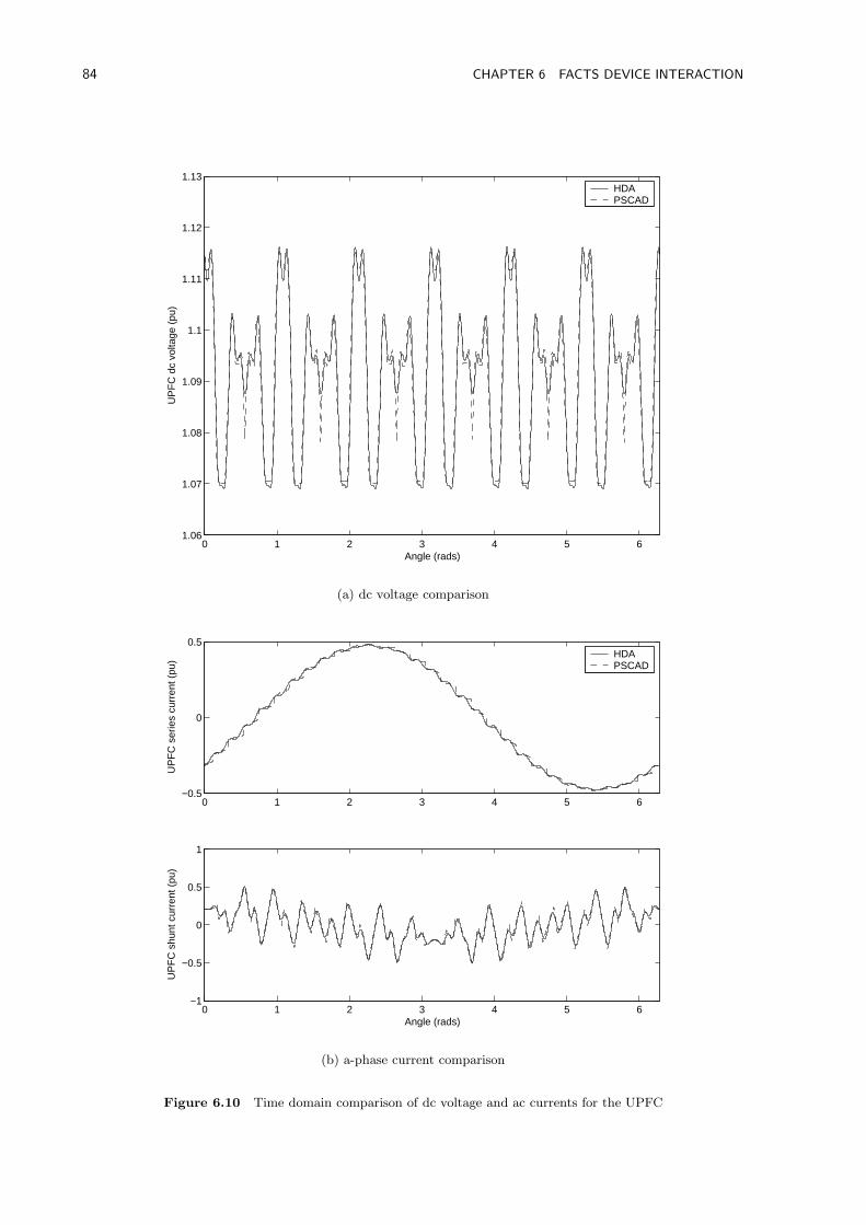
84 CHAPTER 6 FACTS DEVICE INTERACTION
0 1 2 3 4 5 61.06
1.07
1.08
1.09
1.1
1.11
1.12
1.13
Angle (rads)
UP
FC
dc
volta
ge (
pu)
HDAPSCAD
(a) dc voltage comparison
0 1 2 3 4 5 6−0.5
0
0.5
UP
FC
ser
ies
curr
ent (
pu)
0 1 2 3 4 5 6−1
−0.5
0
0.5
1
Angle (rads)
UP
FC
shu
nt c
urre
nt (
pu)
HDAPSCAD
(b) a-phase current comparison
Figure 6.10 Time domain comparison of dc voltage and ac currents for the UPFC
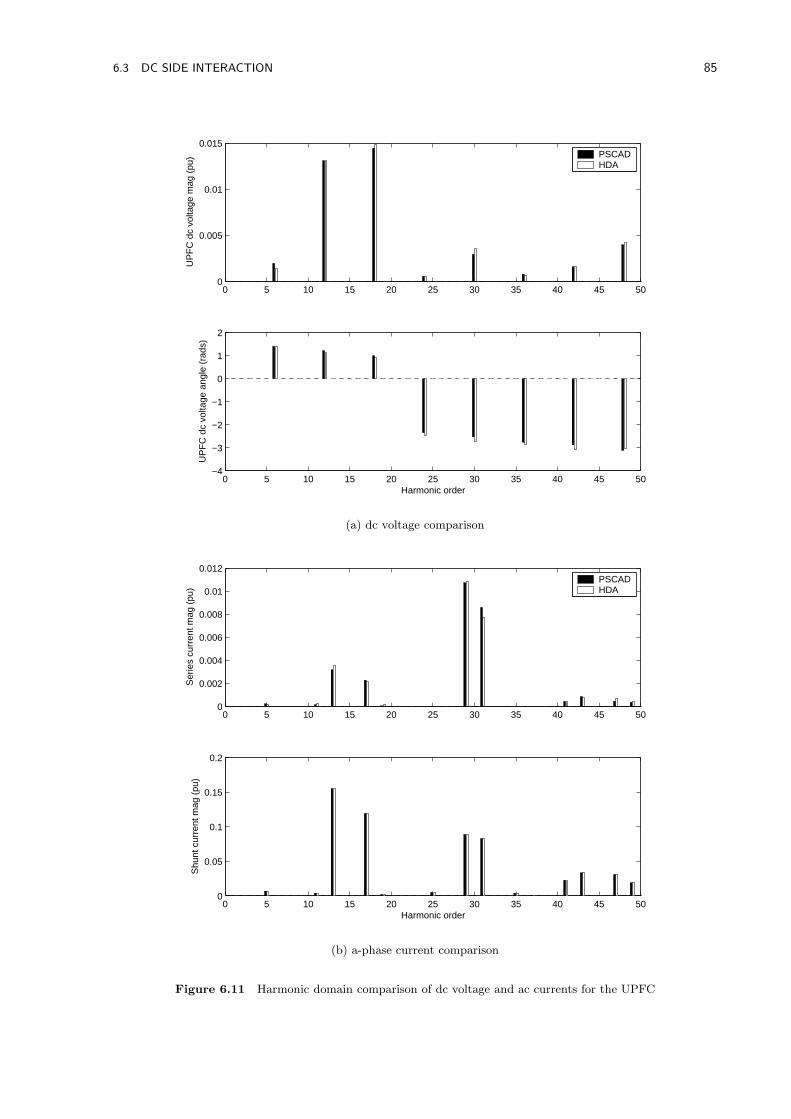
6.3 DC SIDE INTERACTION 85
0 5 10 15 20 25 30 35 40 45 500
0.005
0.01
0.015
UP
FC
dc
volta
ge m
ag (
pu)
0 5 10 15 20 25 30 35 40 45 50−4
−3
−2
−1
0
1
2
Harmonic order
UP
FC
dc
volta
ge a
ngle
(ra
ds)
PSCADHDA
(a) dc voltage comparison
0 5 10 15 20 25 30 35 40 45 500
0.002
0.004
0.006
0.008
0.01
0.012
Ser
ies
curr
ent m
ag (
pu)
0 5 10 15 20 25 30 35 40 45 500
0.05
0.1
0.15
0.2
Harmonic order
Shu
nt c
urre
nt m
ag (
pu)
PSCADHDA
(b) a-phase current comparison
Figure 6.11 Harmonic domain comparison of dc voltage and ac currents for the UPFC
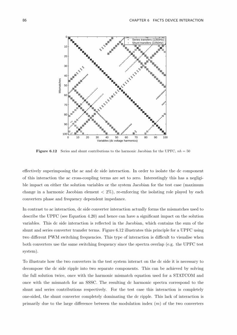
86 CHAPTER 6 FACTS DEVICE INTERACTION
0 10 20 30 40 50 60 70 80 90 100
0
10
20
30
40
50
60
70
80
90
100
Mis
mat
ches
Variables (dc voltage harmonics)
Series transfers (1350Hz)Shunt transfers (2250Hz)
Figure 6.12 Series and shunt contributions to the harmonic Jacobian for the UPFC, nh = 50
effectively superimposing the ac and dc side interaction. In order to isolate the dc component
of this interaction the ac cross-coupling terms are set to zero. Interestingly this has a negligi-
ble impact on either the solution variables or the system Jacobian for the test case (maximum
change in a harmonic Jacobian element < 2%), re-enforcing the isolating role played by each
converters phase and frequency dependent impedance.
In contrast to ac interaction, dc side converter interaction actually forms the mismatches used to
describe the UPFC (see Equation 4.20) and hence can have a significant impact on the solution
variables. This dc side interaction is reflected in the Jacobian, which contains the sum of the
shunt and series converter transfer terms. Figure 6.12 illustrates this principle for a UPFC using
two different PWM switching frequencies. This type of interaction is difficult to visualise when
both converters use the same switching frequency since the spectra overlap (e.g. the UPFC test
system).
To illustrate how the two converters in the test system interact on the dc side it is necessary to
decompose the dc side ripple into two separate components. This can be achieved by solving
the full solution twice, once with the harmonic mismatch equation used for a STATCOM and
once with the mismatch for an SSSC. The resulting dc harmonic spectra correspond to the
shunt and series contributions respectively. For the test case this interaction is completely
one-sided, the shunt converter completely dominating the dc ripple. This lack of interaction is
primarily due to the large difference between the modulation index (m) of the two converters
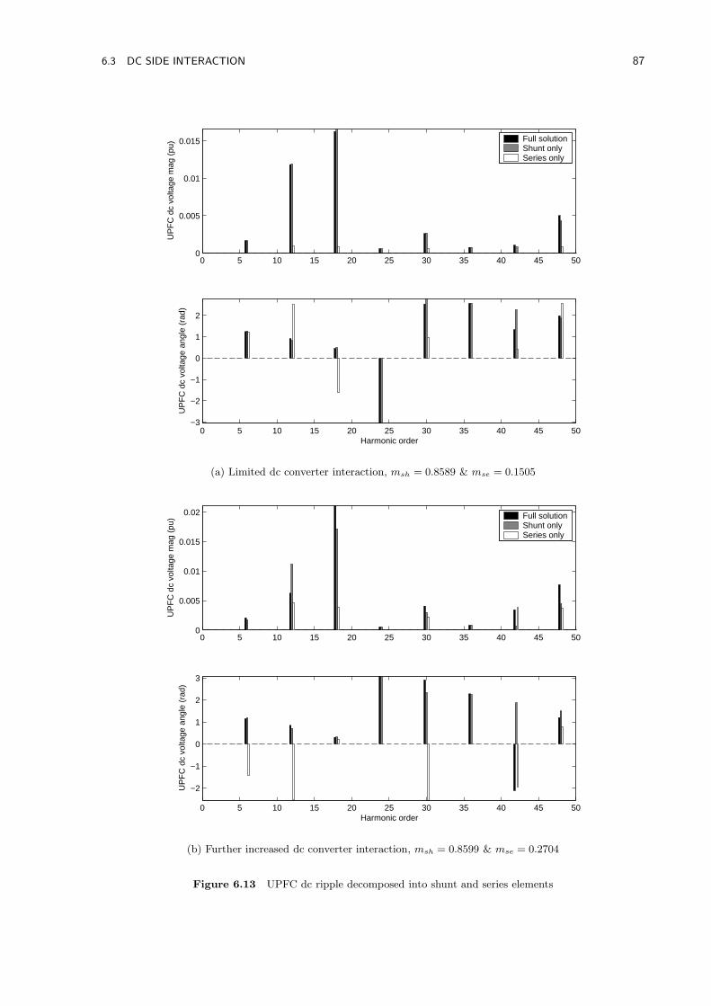
6.3 DC SIDE INTERACTION 87
0 5 10 15 20 25 30 35 40 45 500
0.005
0.01
0.015
UP
FC
dc
volta
ge m
ag (
pu)
0 5 10 15 20 25 30 35 40 45 50−3
−2
−1
0
1
2
Harmonic order
UP
FC
dc
volta
ge a
ngle
(ra
d)
Full solutionShunt onlySeries only
(a) Limited dc converter interaction, msh = 0.8589 & mse = 0.1505
0 5 10 15 20 25 30 35 40 45 500
0.005
0.01
0.015
0.02
UP
FC
dc
volta
ge m
ag (
pu)
0 5 10 15 20 25 30 35 40 45 50
−2
−1
0
1
2
3
Harmonic order
UP
FC
dc
volta
ge a
ngle
(ra
d)
Full solutionShunt onlySeries only
(b) Further increased dc converter interaction, msh = 0.8599 & mse = 0.2704
Figure 6.13 UPFC dc ripple decomposed into shunt and series elements
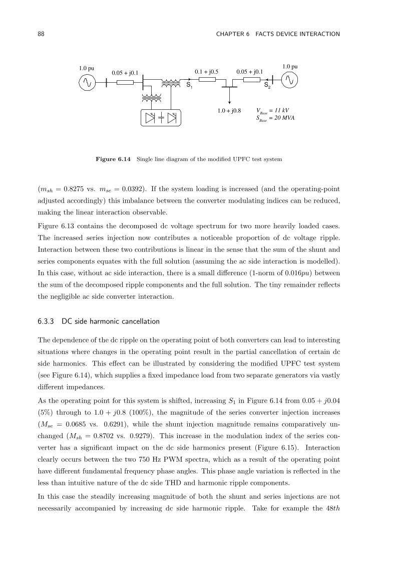
88 CHAPTER 6 FACTS DEVICE INTERACTION
0.05 + j0.1 0.1 + j0.5
1.0 + j0.8
1.0 pu
V Base
= 11 kV
S Base
= 20 MVA
S
2 S
1
1.0 pu 0.05 + j0.1
Figure 6.14 Single line diagram of the modified UPFC test system
(msh = 0.8275 vs. mse = 0.0392). If the system loading is increased (and the operating-point
adjusted accordingly) this imbalance between the converter modulating indices can be reduced,
making the linear interaction observable.
Figure 6.13 contains the decomposed dc voltage spectrum for two more heavily loaded cases.
The increased series injection now contributes a noticeable proportion of dc voltage ripple.
Interaction between these two contributions is linear in the sense that the sum of the shunt and
series components equates with the full solution (assuming the ac side interaction is modelled).
In this case, without ac side interaction, there is a small difference (1-norm of 0.016pu) between
the sum of the decomposed ripple components and the full solution. The tiny remainder reflects
the negligible ac side converter interaction.
6.3.3 DC side harmonic cancellation
The dependence of the dc ripple on the operating point of both converters can lead to interesting
situations where changes in the operating point result in the partial cancellation of certain dc
side harmonics. This effect can be illustrated by considering the modified UPFC test system
(see Figure 6.14), which supplies a fixed impedance load from two separate generators via vastly
different impedances.
As the operating point for this system is shifted, increasing S1 in Figure 6.14 from 0.05 + j0.04
(5%) through to 1.0 + j0.8 (100%), the magnitude of the series converter injection increases
(Mse = 0.0685 vs. 0.6291), while the shunt injection magnitude remains comparatively un-
changed (Msh = 0.8702 vs. 0.9279). This increase in the modulation index of the series con-
verter has a significant impact on the dc side harmonics present (Figure 6.15). Interaction
clearly occurs between the two 750 Hz PWM spectra, which as a result of the operating point
have different fundamental frequency phase angles. This phase angle variation is reflected in the
less than intuitive nature of the dc side THD and harmonic ripple components.
In this case the steadily increasing magnitude of both the shunt and series injections are not
necessarily accompanied by increasing dc side harmonic ripple. Take for example the 48th
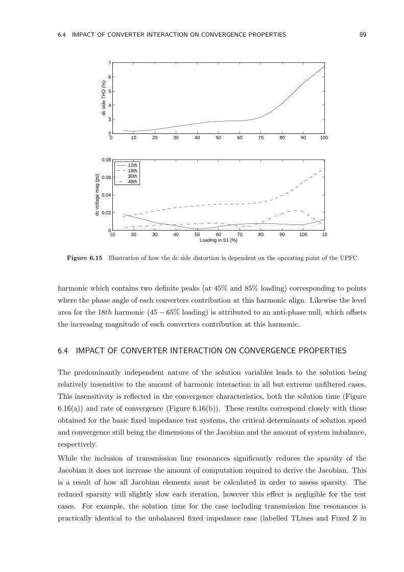
6.4 IMPACT OF CONVERTER INTERACTION ON CONVERGENCE PROPERTIES 89
0 10 20 30 40 50 60 70 80 90 100 2
3
4
5
6
7
dc s
ide
TH
D (
%)
10 20 30 40 50 60 70 80 90 100 100
0.02
0.04
0.06
0.08
dc v
olta
ge m
ag (
pu)
Loading in S1 (%)
12th18th30th48th
Figure 6.15 Illustration of how the dc side distortion is dependent on the operating point of the UPFC
harmonic which contains two definite peaks (at 45% and 85% loading) corresponding to points
where the phase angle of each converters contribution at this harmonic align. Likewise the level
area for the 18th harmonic (45 − 65% loading) is attributed to an anti-phase null, which offsets
the increasing magnitude of each converters contribution at this harmonic.
6.4 IMPACT OF CONVERTER INTERACTION ON CONVERGENCE PROPERTIES
The predominantly independent nature of the solution variables leads to the solution being
relatively insensitive to the amount of harmonic interaction in all but extreme unfiltered cases.
This insensitivity is reflected in the convergence characteristics, both the solution time (Figure
6.16(a)) and rate of convergence (Figure 6.16(b)). These results correspond closely with those
obtained for the basic fixed impedance test systems, the critical determinants of solution speed
and convergence still being the dimensions of the Jacobian and the amount of system imbalance,
respectively.
While the inclusion of transmission line resonances significantly reduces the sparsity of the
Jacobian it does not increase the amount of computation required to derive the Jacobian. This
is a result of how all Jacobian elements must be calculated in order to assess sparsity. The
reduced sparsity will slightly slow each iteration, however this effect is negligible for the test
cases. For example, the solution time for the case including transmission line resonances is
practically identical to the unbalanced fixed impedance case (labelled TLines and Fixed Z in
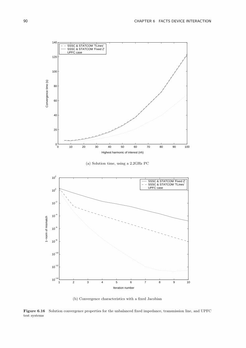
90 CHAPTER 6 FACTS DEVICE INTERACTION
0 10 20 30 40 50 60 70 80 90 1000
20
40
60
80
100
120
140
Highest harmonic of interest (nh)
Con
verg
ence
tim
e (s
)SSSC & STATCOM ’TLines’SSSC & STATCOM ’Fixed Z’UPFC case
(a) Solution time, using a 2.2GHz PC
1 2 3 4 5 6 7 8 9 1010
−14
10−12
10−10
10−8
10−6
10−4
10−2
100
102
Iteration number
1−no
rm o
f mis
mat
ch
SSSC & STATCOM ’Fixed Z’SSSC & STATCOM ’TLines’UPFC case
(b) Convergence characteristics with a fixed Jacobian
Figure 6.16 Solution convergence properties for the unbalanced fixed impedance, transmission line, and UPFCtest systems
6.5 CONCLUSIONS 91
Figure 6.16(a)). Likewise the UPFC case requires approximately the same amount of time as a
single converter fixed impedance case, illustrating how the number of isolated dc busbars is the
major determinant of the Jacobian’s size and hence the solution speed.
Similarly the rate of convergence using a fixed Jacobian is not significantly degraded in the
presence of system resonances. In fact the rate of convergence for test systems containing ac or dc
interaction (TLines and UPFC in Figure 6.16(b)) is superior to that obtained for the unbalanced
fixed impedance case. This stems from how the transmission system considered within this
Chapter has less unbalance than the unrealistic test case used in Chapter 5. Interestingly the
balanced UPFC case converges faster than the balanced single converter case (Figure 5.9); the
cause of this improved convergence has not been definitively identified, however it is likely that
the different control schemes used by the respective FACTS devices contributes to this difference.
6.5 CONCLUSIONS
This chapter has investigated the impact converter interaction has on the proposed harmonic
solution technique. It has demonstrated how increased harmonic interaction does not signifi-
cantly degrade the models performance, either in terms of accuracy or convergence. Moreover
the choice of the dc side voltage as a solution variable has been justified by the near indepen-
dence of each devices’ dc voltage spectrum. This independence in the solution variables does
not necessarily imply a lack of linear ac side interaction, which was observed in ac terminal
quantities. As such the amount of dc voltage interdependence is a useful guide as to whether
and/or where in depth harmonic interaction analysis is required.
The magnitude of any interaction is shown to be dependent on both the operating point and the
composition of the test system, in particular resonant components such as filters and transmission
systems. While the Jacobian reflects these components and the resultant sensitivity in the
harmonic solution, it is not necessarily a good measure of the magnitude of the interaction
present since resonances are not necessarily excited.

Chapter 7
CONTROL SYSTEM LINEARITY
7.1 INTRODUCTION
Previous chapters have focused on the electrical aspects of FACTS device analysis in the har-
monic domain, as such the associated test systems featured heavily filtered control networks and
conservative operating points (i.e. no over-modulation). Both of these common assumptions
improve system linearity by idealising the PWM process. This results in improved computa-
tional efficiency, something which is advantageous for multi-converter studies requiring a large
system Jacobian. This chapter considers the impact these common assumptions have on both
the accuracy and convergence of the proposed iterative solution, before discussing where these
control assumptions are appropriate.
7.2 DISTORTED CONTROL FEEDBACK
While the PI controller and the associated filters are assumed within this thesis to behave in
a linear fashion, the output from this block has a significant impact on the PWM process (a
primary source of non-linearity). For heavily filtered control cases this non-linearity is limited to
the switching spectrums dependence on the power-flow control variables αdc and mdc, leaving the
harmonic transfers perfectly linear. Removing this isolation contributes additional non-linear
harmonic transfers which complicate the solution by increasing the Jacobian size and reducing
the rate of convergence. The resultant reduction in efficiency makes the assumption of a heavily
filtered feedback network particularly attractive. In order to assess the accuracy of this common
assumption this section presents the impact of introducing PWM distortion to an SSSC.
7.2.1 Feedback mechanism
The introduction of harmonic distortion to the PWM process leads to variation in the switching
instants, which in turn generates non-characteristic ac side harmonics. Figure 7.1 illustrates this
effect for the ac terminal current spectra of the SSSC test system (see Appendix B.3). In this
case the sinusoidal modulating function has been heavily distorted by a second harmonic ripple
(10%) in the control angle (α). Since the introduced distortion is modulated by the switching
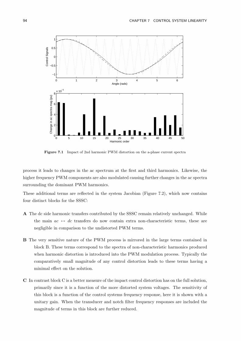
94 CHAPTER 7 CONTROL SYSTEM LINEARITY
0 1 2 3 4 5 6
−1
−0.5
0
0.5
1
Angle (rads)
Con
trol
Sig
nals
0 5 10 15 20 25 30 35 40 45 500
2
4
6
8x 10
−3
Harmonic order
Cha
nge
in a
c sp
ectr
a m
ag (
pu)
Figure 7.1 Impact of 2nd harmonic PWM distortion on the a-phase current spectra
process it leads to changes in the ac spectrum at the first and third harmonics. Likewise, the
higher frequency PWM components are also modulated causing further changes in the ac spectra
surrounding the dominant PWM harmonics.
These additional terms are reflected in the system Jacobian (Figure 7.2), which now contains
four distinct blocks for the SSSC:
A The dc side harmonic transfers contributed by the SSSC remain relatively unchanged. While
the main ac ↔ dc transfers do now contain extra non-characteristic terms, these are
negligible in comparison to the undistorted PWM terms.
B The very sensitive nature of the PWM process is mirrored in the large terms contained in
block B. These terms correspond to the spectra of non-characteristic harmonics produced
when harmonic distortion is introduced into the PWM modulation process. Typically the
comparatively small magnitude of any control distortion leads to these terms having a
minimal effect on the solution.
C In contrast block C is a better measure of the impact control distortion has on the full solution,
primarily since it is a function of the more distorted system voltages. The sensitivity of
this block is a function of the control systems frequency response, here it is shown with a
unitary gain. When the transducer and notch filter frequency responses are included the
magnitude of terms in this block are further reduced.
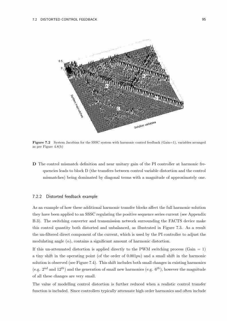
7.2 DISTORTED CONTROL FEEDBACK 95
Figure 7.2 System Jacobian for the SSSC system with harmonic control feedback (Gain=1), variables arrangedas per Figure 4.8(b)
D The control mismatch definition and near unitary gain of the PI controller at harmonic fre-
quencies leads to block D (the transfers between control variable distortion and the control
mismatches) being dominated by diagonal terms with a magnitude of approximately one.
7.2.2 Distorted feedback example
As an example of how these additional harmonic transfer blocks affect the full harmonic solution
they have been applied to an SSSC regulating the positive sequence series current (see Appendix
B.3). The switching converter and transmission network surrounding the FACTS device make
this control quantity both distorted and unbalanced, as illustrated in Figure 7.3. As a result
the un-filtered direct component of the current, which is used by the PI controller to adjust the
modulating angle (α), contains a significant amount of harmonic distortion.
If this un-attenuated distortion is applied directly to the PWM switching process (Gain = 1)
a tiny shift in the operating point (of the order of 0.001pu) and a small shift in the harmonic
solution is observed (see Figure 7.4). This shift includes both small changes in existing harmonics
(e.g. 2nd and 12th) and the generation of small new harmonics (e.g. 6th), however the magnitude
of all these changes are very small.
The value of modelling control distortion is further reduced when a realistic control transfer
function is included. Since controllers typically attenuate high order harmonics and often include
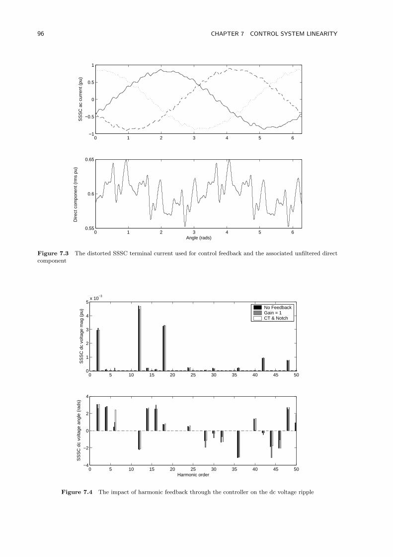
96 CHAPTER 7 CONTROL SYSTEM LINEARITY
0 1 2 3 4 5 6−1
−0.5
0
0.5
1
SS
SC
ac
curr
ent (
pu)
0 1 2 3 4 5 60.55
0.6
0.65
Angle (rads)
Dire
ct c
ompo
nent
(rm
s pu
)
Figure 7.3 The distorted SSSC terminal current used for control feedback and the associated unfiltered directcomponent
0 5 10 15 20 25 30 35 40 45 500
1
2
3
4
5x 10
−3
SS
SC
dc
volta
ge m
ag (
pu)
0 5 10 15 20 25 30 35 40 45 50−4
−2
0
2
4
Harmonic order
SS
SC
dc
volta
ge a
ngle
(ra
ds)
No FeedbackGain = 1CT & Notch
Figure 7.4 The impact of harmonic feedback through the controller on the dc voltage ripple
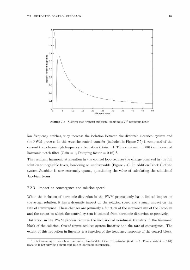
7.2 DISTORTED CONTROL FEEDBACK 97
0 5 10 15 20 25 30 35 40 45 500
0.1
0.2
0.3
0.4
0.5
0.6
0.7
0.8
0.9
1
Harmonic order
Tra
nsfe
r fu
nctio
n m
agni
tude
Figure 7.5 Control loop transfer function, including a 2nd harmonic notch
low frequency notches, they increase the isolation between the distorted electrical system and
the PWM process. In this case the control transfer (included in Figure 7.5) is composed of the
current transducers high frequency attenuation (Gain = 1, Time constant = 0.001) and a second
harmonic notch filter (Gain = 1, Damping factor = 0.16) 1.
The resultant harmonic attenuation in the control loop reduces the change observed in the full
solution to negligible levels, bordering on unobservable (Figure 7.4). In addition Block C of the
system Jacobian is now extremely sparse, questioning the value of calculating the additional
Jacobian terms.
7.2.3 Impact on convergence and solution speed
While the inclusion of harmonic distortion in the PWM process only has a limited impact on
the actual solution, it has a dramatic impact on the solution speed and a small impact on the
rate of convergence. These changes are primarily a function of the increased size of the Jacobian
and the extent to which the control system is isolated from harmonic distortion respectively.
Distortion in the PWM process requires the inclusion of non-linear transfers in the harmonic
block of the solution, this of course reduces system linearity and the rate of convergence. The
extent of this reduction in linearity is a function of the frequency response of the control block.
1It is interesting to note how the limited bandwidth of the PI controller (Gain = 1, Time constant = 0.01)leads to it not playing a significant role at harmonic frequencies.
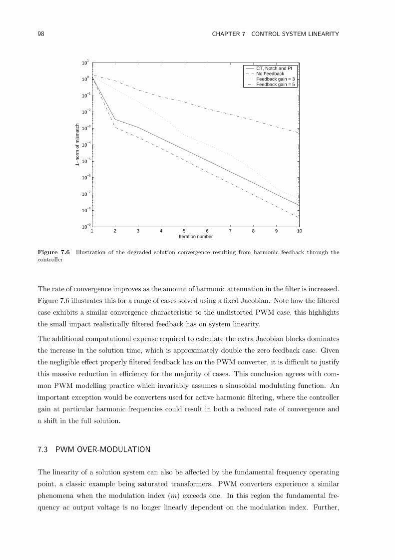
98 CHAPTER 7 CONTROL SYSTEM LINEARITY
1 2 3 4 5 6 7 8 9 1010
−9
10−8
10−7
10−6
10−5
10−4
10−3
10−2
10−1
100
101
Iteration number
1−no
rm o
f mis
mat
ch
CT, Notch and PINo FeedbackFeedback gain = 3Feedback gain = 5
Figure 7.6 Illustration of the degraded solution convergence resulting from harmonic feedback through thecontroller
The rate of convergence improves as the amount of harmonic attenuation in the filter is increased.
Figure 7.6 illustrates this for a range of cases solved using a fixed Jacobian. Note how the filtered
case exhibits a similar convergence characteristic to the undistorted PWM case, this highlights
the small impact realistically filtered feedback has on system linearity.
The additional computational expense required to calculate the extra Jacobian blocks dominates
the increase in the solution time, which is approximately double the zero feedback case. Given
the negligible effect properly filtered feedback has on the PWM converter, it is difficult to justify
this massive reduction in efficiency for the majority of cases. This conclusion agrees with com-
mon PWM modelling practice which invariably assumes a sinusoidal modulating function. An
important exception would be converters used for active harmonic filtering, where the controller
gain at particular harmonic frequencies could result in both a reduced rate of convergence and
a shift in the full solution.
7.3 PWM OVER-MODULATION
The linearity of a solution system can also be affected by the fundamental frequency operating
point, a classic example being saturated transformers. PWM converters experience a similar
phenomena when the modulation index (m) exceeds one. In this region the fundamental fre-
quency ac output voltage is no longer linearly dependent on the modulation index. Further,
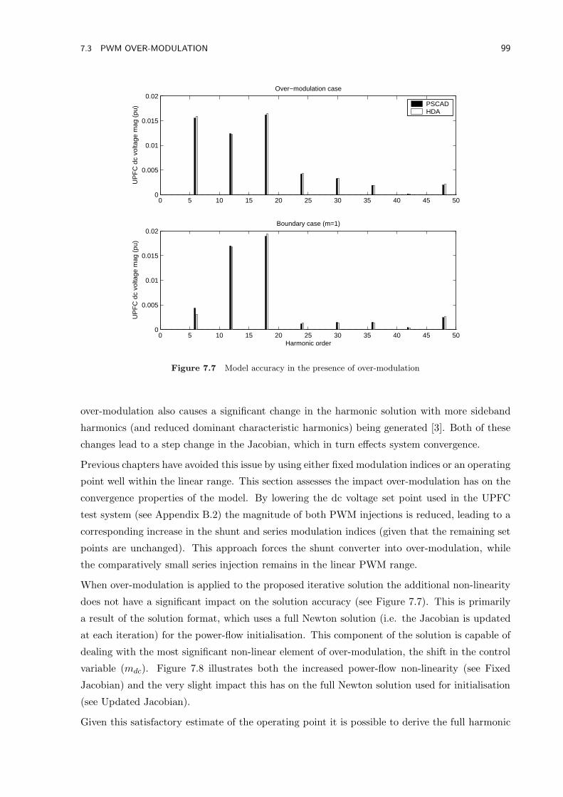
7.3 PWM OVER-MODULATION 99
0 5 10 15 20 25 30 35 40 45 500
0.005
0.01
0.015
0.02Over−modulation case
UP
FC
dc
volta
ge m
ag (
pu)
0 5 10 15 20 25 30 35 40 45 500
0.005
0.01
0.015
0.02Boundary case (m=1)
Harmonic order
UP
FC
dc
volta
ge m
ag (
pu)
PSCADHDA
Figure 7.7 Model accuracy in the presence of over-modulation
over-modulation also causes a significant change in the harmonic solution with more sideband
harmonics (and reduced dominant characteristic harmonics) being generated [3]. Both of these
changes lead to a step change in the Jacobian, which in turn effects system convergence.
Previous chapters have avoided this issue by using either fixed modulation indices or an operating
point well within the linear range. This section assesses the impact over-modulation has on the
convergence properties of the model. By lowering the dc voltage set point used in the UPFC
test system (see Appendix B.2) the magnitude of both PWM injections is reduced, leading to a
corresponding increase in the shunt and series modulation indices (given that the remaining set
points are unchanged). This approach forces the shunt converter into over-modulation, while
the comparatively small series injection remains in the linear PWM range.
When over-modulation is applied to the proposed iterative solution the additional non-linearity
does not have a significant impact on the solution accuracy (see Figure 7.7). This is primarily
a result of the solution format, which uses a full Newton solution (i.e. the Jacobian is updated
at each iteration) for the power-flow initialisation. This component of the solution is capable of
dealing with the most significant non-linear element of over-modulation, the shift in the control
variable (mdc). Figure 7.8 illustrates both the increased power-flow non-linearity (see Fixed
Jacobian) and the very slight impact this has on the full Newton solution used for initialisation
(see Updated Jacobian).
Given this satisfactory estimate of the operating point it is possible to derive the full harmonic
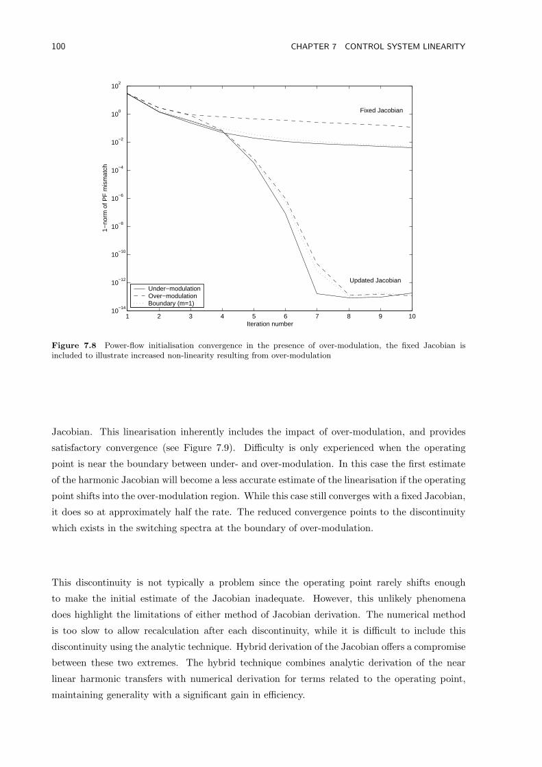
100 CHAPTER 7 CONTROL SYSTEM LINEARITY
1 2 3 4 5 6 7 8 9 1010
−14
10−12
10−10
10−8
10−6
10−4
10−2
100
102
Iteration number
1−no
rm o
f PF
mis
mat
ch
Under−modulationOver−modulationBoundary (m=1)
Fixed Jacobian
Updated Jacobian
Figure 7.8 Power-flow initialisation convergence in the presence of over-modulation, the fixed Jacobian isincluded to illustrate increased non-linearity resulting from over-modulation
Jacobian. This linearisation inherently includes the impact of over-modulation, and provides
satisfactory convergence (see Figure 7.9). Difficulty is only experienced when the operating
point is near the boundary between under- and over-modulation. In this case the first estimate
of the harmonic Jacobian will become a less accurate estimate of the linearisation if the operating
point shifts into the over-modulation region. While this case still converges with a fixed Jacobian,
it does so at approximately half the rate. The reduced convergence points to the discontinuity
which exists in the switching spectra at the boundary of over-modulation.
This discontinuity is not typically a problem since the operating point rarely shifts enough
to make the initial estimate of the Jacobian inadequate. However, this unlikely phenomena
does highlight the limitations of either method of Jacobian derivation. The numerical method
is too slow to allow recalculation after each discontinuity, while it is difficult to include this
discontinuity using the analytic technique. Hybrid derivation of the Jacobian offers a compromise
between these two extremes. The hybrid technique combines analytic derivation of the near
linear harmonic transfers with numerical derivation for terms related to the operating point,
maintaining generality with a significant gain in efficiency.
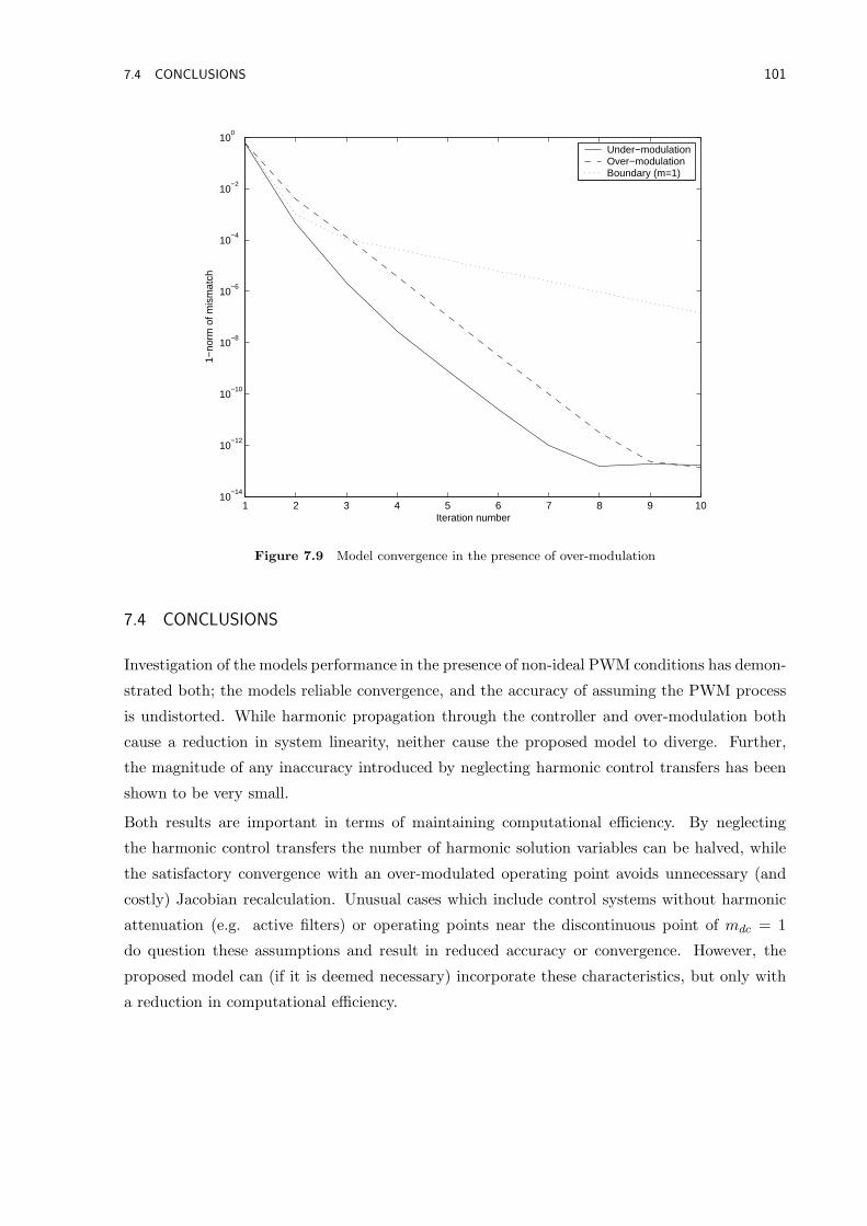
7.4 CONCLUSIONS 101
1 2 3 4 5 6 7 8 9 1010
−14
10−12
10−10
10−8
10−6
10−4
10−2
100
Iteration number
1−no
rm o
f mis
mat
ch
Under−modulationOver−modulationBoundary (m=1)
Figure 7.9 Model convergence in the presence of over-modulation
7.4 CONCLUSIONS
Investigation of the models performance in the presence of non-ideal PWM conditions has demon-
strated both; the models reliable convergence, and the accuracy of assuming the PWM process
is undistorted. While harmonic propagation through the controller and over-modulation both
cause a reduction in system linearity, neither cause the proposed model to diverge. Further,
the magnitude of any inaccuracy introduced by neglecting harmonic control transfers has been
shown to be very small.
Both results are important in terms of maintaining computational efficiency. By neglecting
the harmonic control transfers the number of harmonic solution variables can be halved, while
the satisfactory convergence with an over-modulated operating point avoids unnecessary (and
costly) Jacobian recalculation. Unusual cases which include control systems without harmonic
attenuation (e.g. active filters) or operating points near the discontinuous point of mdc = 1
do question these assumptions and result in reduced accuracy or convergence. However, the
proposed model can (if it is deemed necessary) incorporate these characteristics, but only with
a reduction in computational efficiency.

Chapter 8
CONCLUSIONS AND FUTURE WORK
8.1 CONCLUSIONS
The application of PWM switching to modern power system equipment has provided a wealth
of control possibilities, it has not however lessened the requirement for accurate harmonic simu-
lation tools. A review of existing harmonic analysis techniques revealed a bias toward older line
commutated technologies and basic linearised PWM modelling. Using this review as a basis, a
comprehensive Newton solution algorithm, tailored to PWM FACTS devices, has been proposed.
The format adopted allows multiple interconnected PWM converters, configured as FACTS
devices, to be comprehensively characterised in the steady-state. To achieve this the proposed
formulation incorporates both fundamental and harmonic frequency variables in a single solution
set, the size of which is minimised by using a novel dc side harmonic formulation based on current
mismatches. Nonetheless, both the power-flow and harmonic solutions reflect the full three-phase
ac system and are capable of analyzing non-characteristic harmonic distortion resulting from
system imbalance. The full harmonic solution, which is initialised using a three-phase power-
flow, has been shown to reliably converge for a range of test systems incorporating transmission
line resonance and multiple PWM converters. The results have subsequently been validated
against time domain simulation; excellent agreement being obtained at both fundamental and
harmonic frequencies.
The modular PWM converter block has been successfully applied to shunt, series and hybrid
FACTS devices using a combination of harmonic current and voltage sources. These distorting
sources interact across a linear ac system admittance leading to converter interdependence. This
interdependence has a considerable impact on ac side quantities but, as a result of the converters
phase and frequency dependent impedance, not on the dc side quantities used as the solution
variables. This independence provides further justification for the use of dc side quantities as
solution variables. Interestingly the Jacobian is not a good visual measure of this independence,
but instead is dominated by small but sensitive resonances. DC side harmonic interaction
has also been demonstrated for the UPFC. In this case the Jacobian better reflects the linear
combination of each individual converters harmonic lattice, making it a useful measure of dc
side harmonic interaction.
104 CHAPTER 8 CONCLUSIONS AND FUTURE WORK
Both these harmonic interaction mechanisms are, in the absence of control distortion, perfectly
linear. As such, an iterative solution is only required because of the non-linear interaction
between the harmonic and fundamental frequency solutions. For idealised cases the magnitude
of this harmonic induced operating point shift is small, however the presence of system imbalance
leads to a noticeable shift. In these non-ideal cases (e.g. small dc side capacitor or large ac current
imbalance) the operating point shift should be included in the solution, either with an iterative
solution or with a linearised power-flow equivalent (small-signal cases only).
Investigation into the control network confirmed both the model’s reliable convergence, and the
accuracy of assuming the control system is immune to harmonic distortion. Both results im-
prove the generality of the proposed model; the reliable convergence permits over-modulation
to be considered, while the assumption of controller immunity greatly improves computational
efficiency. This improved efficiency is particularly relevant to systems containing multiple dis-
tributed FACTS devices, where it is necessary to simulate many interconnected converters in
order to assess the aggregate impact on the system.
8.2 FUTURE WORK
The research detailed in this thesis could be extended in a number of ways, both in terms of
improving the proposed model and using the results to develop more efficient solution techniques.
8.2.1 Iterative model improvements
This thesis has described and validated a novel solution framework for PWM FACTS devices,
as such the emphasis has been placed on investigating the characteristics of the proposed model,
rather than an optimal implementation. While the MATLAB implementation developed is much
faster than an equivalent time domain solution, there is still significant room for improvement.
The following refinements are particularly important:
Coding environment The MATLAB environment has proved satisfactory for model evalua-
tion, however it is not a very efficient modelling environment. This restriction becomes
apparent when the model needs to handle the large amounts of data associated with system
level studies (e.g. massive system matrices and variable vectors). It would therefore be
advantageous to migrate the proposed technique into a more efficient coding environment.
Jacobian derivation In terms of efficiency the largest gains would be obtained by developing
analytic expressions for the system Jacobian. Of particular importance are the large har-
monic transfer blocks. These large blocks could be described relatively easily and provide
a significant efficiency gain, without compromising generality. In contrast analytic deriva-
tion for the control blocks would not necessarily be as rewarding, since these complex
very non-linear blocks only contribute a small proportion of the Jacobian. Thus a hybrid
derivation could improve efficiency without compromising generality or modularity.
8.2 FUTURE WORK 105
The extent to which each FACTS device and the surrounding network is modelled could be
improved by considering the following aspects:
AC component models For validation purposes the solution technique has been implemented
using basic power-flow and harmonic models (with the exception of transmission lines).
Ideally the proposed dc mismatch technique should be interfaced with an existing power-
flow program with more advanced component models (e.g. delta connections and off-
tap transformers). Likewise, the harmonic frequency models and the associated system
admittance formulation could easily be refined by incorporating existing direct harmonic
analysis models and techniques.
Transformer saturation Saturated transformers, like FACTS devices, behave in a non-linear
fashion which can be characterised using harmonic domain techniques. Complex conjugate
models of this type already exist and there is no reason why these models could not be
transferred to the positive frequency approach and integrated with the proposed solution.
Asynchronous PWM The assumption of an ideal PLL is very important in HDA since it
generates both a constant frequency and angle reference. These references lead to a syn-
chronous PWM process. While steady-state harmonic PLL distortion could be incorpo-
rated within this synchronous framework (in a similar fashion to PWM distortion), the
applicability of harmonic domain techniques to asynchronous situations has yet to be in-
vestigated.
8.2.2 Extension to other PWM devices
Other FACTS devices
The modular formulation of the proposed model makes it relatively simple to extend the existing
analysis to other FACTS devices which share the PWM converter block. A large range of ac
and dc side combinations could be considered using the existing components. For example
an Interline Power Flow Control (IPFC) could be modelled by combining two series PWM
converters, which share a dc bus. This harmonic representation could then be combined with the
appropriate power-flow and control mismatches (many of which could be derived from existing
mismatches) to form the full steady-state solution.
The existing solution framework is however limited to hard switched converters which have one
dc port and one three-phase ac port. The formulation is not presently capable of modelling the
complex dc side configurations associated with multi-level converter systems. These systems
have multiple dc ports corresponding to each voltage level and present an interesting extension
to existing harmonic analysis techniques.
106 CHAPTER 8 CONCLUSIONS AND FUTURE WORK
Active filters
Active harmonic filtering is based on the principle of varying a converters modulation scheme
such that anti-phase harmonic currents are injected. These currents in turn mitigate exist-
ing distortion. This procedure makes the non-linear modulation process heavily dependent on
harmonic variables (via the control loop), something which the proposed model is specifically
designed to represent. Given the calculation of the switching angles (and the associated transfer
function) is internalised, it would be relatively easy to substitute an appropriate modulation
technique without effecting the main dc side harmonic transfers.
PWM motor drives
At lower voltage levels PWM converters are often used as part of motor drive systems. The
PWM transfers described within this thesis are directly applicable to this situation. Indeed, the
shared dc busbar configuration used to model the UPFC could easily be modified to represent the
rectifier and inverter components of a variable speed motor drive system. Likewise this structure
is also relevant to wind energy systems utilising either doubly-fed induction or variable frequency
synchronous generators.
8.2.3 Large distributed system studies
It is important to view all these improvements in context of PWM devices, rather than HVdc
equipment1. Whereas it may be appropriate to model large converters in an extremely detailed
fashion (e.g. including transformer saturation and thorough control modelling) this is not neces-
sarily important, or indeed feasible, for distributed PWM devices. It is important that the small
accuracy improvements available are balanced against the associated loss in efficiency. Further
these small accuracy improvements must be viewed in terms of the inherent difficulties involved
in modelling the interconnecting transmission network. For most cases uncertainty regarding the
harmonic impedance of loads and transmission circuits will question whether minor converter
details are the limiting factor for harmonic simulation accuracy.
With this in mind a distinction should be drawn between modelling an isolated FACTS devices in
minute detail, and modelling the aggregate effect of many converters. While harmonic domain
techniques are capable of undertaking detailed studies, the harmonic domain’s real strength
remains with system level studies. Studies of this type require elegant solutions which take
advantage of appropriate simplifying assumptions. The research described in this thesis has
used a detailed PWM converter model to illustrate some of these critical assumptions. Looking
forward, further investigation is required into efficient/approximate multi-converter modelling
techniques which can be applied to large scale distributed networks.
1The vast majority of PWM devices are relatively small and widely distributed, in contrast HVdc systems arelarge but rare.
Appendix A
PUBLISHED PAPERS
The following papers have either been published or presented in conjunction with the work
described within this thesis:
1. C.D. Collins, G.N. Bathurst, N.R. Watson, and A.R. Wood. Harmonic domain approach
to STATCOM modelling. IEE Proc.-Gener. Transm. Distrib., 152(2):194-200, Mar. 2005.
2. C. Collins, N. Watson, and A. Wood. UPFC modeling in the harmonic domain. IEEE
Transactions on Power Delivery, 21(2):933-938, Apr. 2006.
3. C.D. Collins, A.R. Wood, and N.R. Watson. Unbalanced STATCOM analysis in the
harmonic domain. Proceedings of the 11th ICHQP, 1:232-237, Lake Placid, 2004.
4. C.D. Collins, N.R. Watson, and A.R. Wood. FACTS device interaction in the harmonic
domain. Proceedings of AUPEC05, 1:243-247, Hobart, 2005.
5. C.D. Collins, N.R. Watson, and A.R. Wood. Unbalanced SSSC Modelling in the Harmonic
Domain. Proceedings of IPEC05, Singapore, 2005.

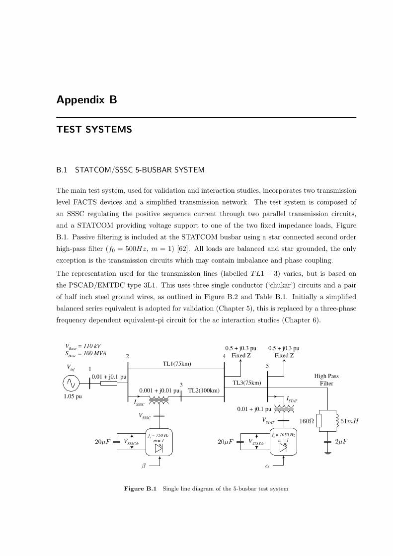
Appendix B
TEST SYSTEMS
B.1 STATCOM/SSSC 5-BUSBAR SYSTEM
The main test system, used for validation and interaction studies, incorporates two transmission
level FACTS devices and a simplified transmission network. The test system is composed of
an SSSC regulating the positive sequence current through two parallel transmission circuits,
and a STATCOM providing voltage support to one of the two fixed impedance loads, Figure
B.1. Passive filtering is included at the STATCOM busbar using a star connected second order
high-pass filter (f0 = 500Hz, m = 1) [62]. All loads are balanced and star grounded, the only
exception is the transmission circuits which may contain imbalance and phase coupling.
The representation used for the transmission lines (labelled TL1 − 3) varies, but is based on
the PSCAD/EMTDC type 3L1. This uses three single conductor (‘chukar’) circuits and a pair
of half inch steel ground wires, as outlined in Figure B.2 and Table B.1. Initially a simplified
balanced series equivalent is adopted for validation (Chapter 5), this is replaced by a three-phase
frequency dependent equivalent-pi circuit for the ac interaction studies (Chapter 6).
I SSSC
0.001 + j0.01 pu
I STAT
TL1(75km)
TL2(100km)
0.01 + j0.1 pu
0.5 + j0.3 pu
Fixed Z
0.5 + j0.3 pu
Fixed Z
TL3(75km)
V inf
0.01 + j0.1 pu
1.05 pu
V Base
= 110 kV
S Base
= 100 MVA
V SSSC V
STAT
V STATdc
V SSSCdc
f s = 750 Hz
m = 1
f s = 1050 Hz
m = 1
1
2
3
4
5
High Pass
Filter
20µF
β
20µF
α
160Ω 51mH
2µF
Figure B.1 Single line diagram of the 5-busbar test system
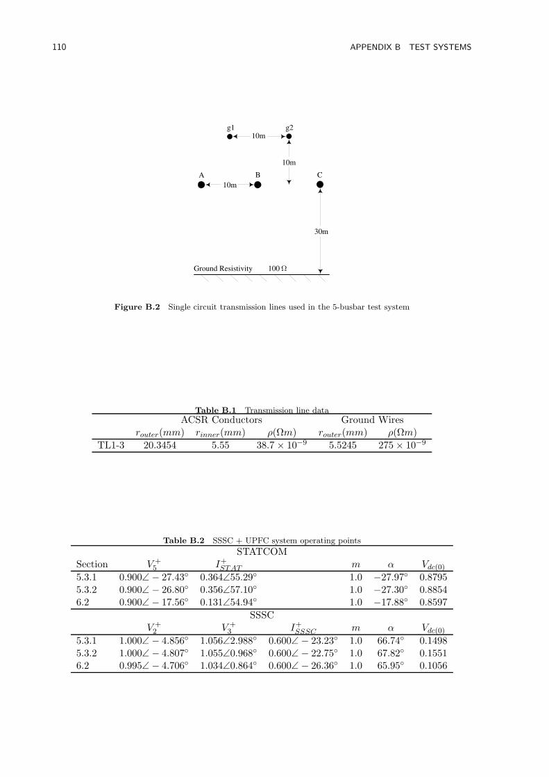
110 APPENDIX B TEST SYSTEMS
10m
10m
10m
A B C
g1 g2
30m
Ground Resistivity 100 Ω
Figure B.2 Single circuit transmission lines used in the 5-busbar test system
Table B.1 Transmission line dataACSR Conductors Ground Wires
router(mm) rinner(mm) ρ(Ωm) router(mm) ρ(Ωm)
TL1-3 20.3454 5.55 38.7 × 10⁻⁹ 5.5245 275 × 10−9
Table B.2 SSSC + UPFC system operating points
STATCOMSection V +
5 I+STAT m α Vdc(0)
5.3.1 0.900∠ − 27.43 0.364∠55.29 1.0 −27.97 0.87955.3.2 0.900∠ − 26.80 0.356∠57.10 1.0 −27.30 0.88546.2 0.900∠ − 17.56 0.131∠54.94 1.0 −17.88 0.8597
SSSCV +
2 V +3 I+
SSSC m α Vdc(0)5.3.1 1.000∠ − 4.856 1.056∠2.988 0.600∠ − 23.23 1.0 66.74 0.14985.3.2 1.000∠ − 4.807 1.055∠0.968 0.600∠ − 22.75 1.0 67.82 0.15516.2 0.995∠ − 4.706 1.034∠0.864 0.600∠ − 26.36 1.0 65.95 0.1056
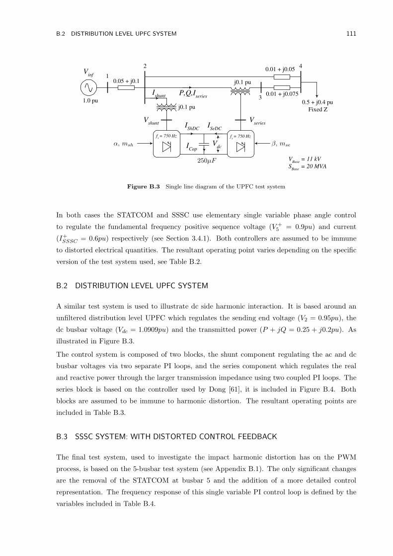
B.2 DISTRIBUTION LEVEL UPFC SYSTEM 111
V series
P,Q,I series
V dc
I ShDC
I SeDC
I Cap
V shunt
I shunt
V inf
0.05 + j0.1
0.01 + j0.05
0.01 + j0.075
0.5 + j0.4 pu
Fixed Z j0.1 pu
j0.1 pu 1
f s = 750 Hz f
s = 750 Hz
1.0 pu
V Base
= 11 kV
S Base
= 20 MVA
2
3
4
α, msh β, mse
250µF
Figure B.3 Single line diagram of the UPFC test system
In both cases the STATCOM and SSSC use elementary single variable phase angle control
to regulate the fundamental frequency positive sequence voltage (V +5 = 0.9pu) and current
(I+SSSC = 0.6pu) respectively (see Section 3.4.1). Both controllers are assumed to be immune
to distorted electrical quantities. The resultant operating point varies depending on the specific
version of the test system used, see Table B.2.
B.2 DISTRIBUTION LEVEL UPFC SYSTEM
A similar test system is used to illustrate dc side harmonic interaction. It is based around an
unfiltered distribution level UPFC which regulates the sending end voltage (V2 = 0.95pu), the
dc busbar voltage (Vdc = 1.0909pu) and the transmitted power (P + jQ = 0.25 + j0.2pu). As
illustrated in Figure B.3.
The control system is composed of two blocks, the shunt component regulating the ac and dc
busbar voltages via two separate PI loops, and the series component which regulates the real
and reactive power through the larger transmission impedance using two coupled PI loops. The
series block is based on the controller used by Dong [61], it is included in Figure B.4. Both
blocks are assumed to be immune to harmonic distortion. The resultant operating points are
included in Table B.3.
B.3 SSSC SYSTEM: WITH DISTORTED CONTROL FEEDBACK
The final test system, used to investigate the impact harmonic distortion has on the PWM
process, is based on the 5-busbar test system (see Appendix B.1). The only significant changes
are the removal of the STATCOM at busbar 5 and the addition of a more detailed control
representation. The frequency response of this single variable PI control loop is defined by the
variables included in Table B.4.
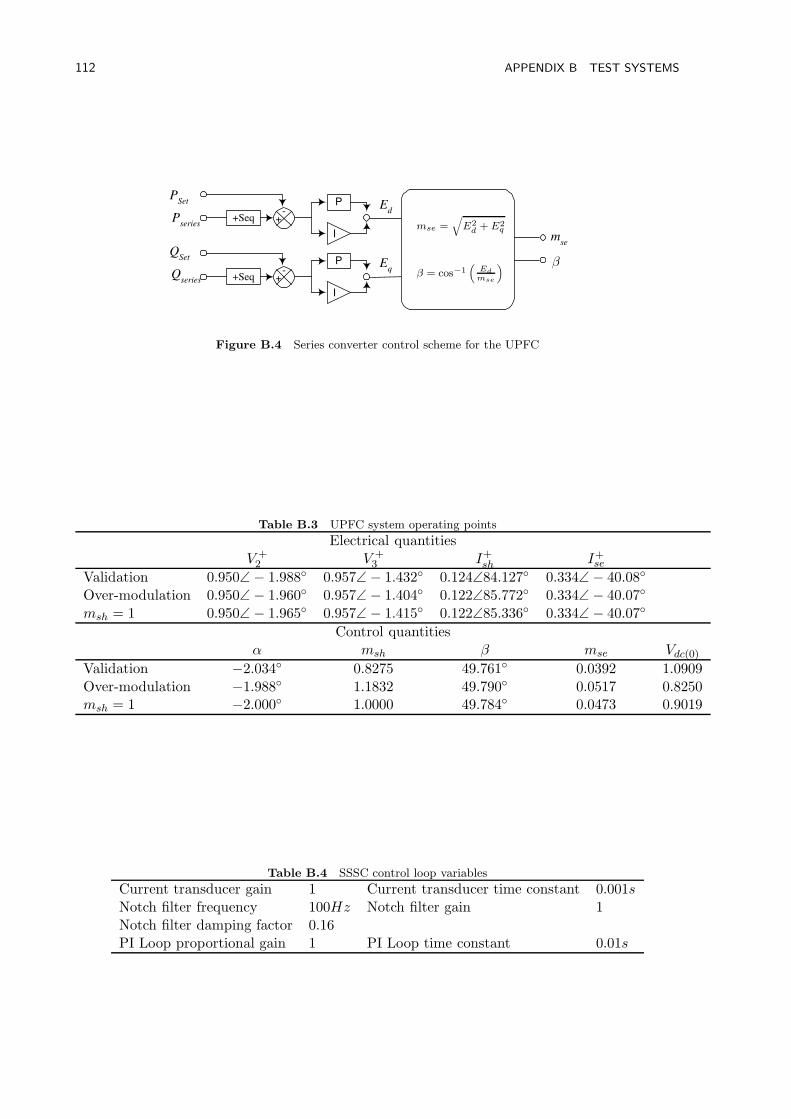
112 APPENDIX B TEST SYSTEMS
+Seq
P
I
+ -
P Set
P series
E d
Q Set
Q series
m se
E q
+Seq
P
I
+ -
β
mse =√
E2d
+ E2q
β = cos−1(Edmse
)
Figure B.4 Series converter control scheme for the UPFC
Table B.3 UPFC system operating points
Electrical quantitiesV +
2 V +3 I+
sh I+se
Validation 0.950∠ − 1.988 0.957∠ − 1.432 0.124∠84.127 0.334∠ − 40.08
Over-modulation 0.950∠ − 1.960 0.957∠ − 1.404 0.122∠85.772 0.334∠ − 40.07
msh = 1 0.950∠ − 1.965 0.957∠ − 1.415 0.122∠85.336 0.334∠ − 40.07
Control quantitiesα msh β mse Vdc(0)
Validation −2.034 0.8275 49.761 0.0392 1.0909Over-modulation −1.988 1.1832 49.790 0.0517 0.8250msh = 1 −2.000 1.0000 49.784 0.0473 0.9019
Table B.4 SSSC control loop variables
Current transducer gain 1 Current transducer time constant 0.001sNotch filter frequency 100Hz Notch filter gain 1Notch filter damping factor 0.16PI Loop proportional gain 1 PI Loop time constant 0.01s
Appendix C
TRANSMISSION LINE MODELLING
The phase to phase coupling, imbalance and harmonic resonances present in transmission systems
play a critical role in the propagation of harmonic distortion. As such it is important that these
transmission line phenomena are included in the harmonic solution. The range of modelling
approaches available and the difficulties involved in validating these models makes including
these phenomena anything but trivial. To a large extent this thesis avoids these problems by
adopting the PSCAD/EMTDC frequency dependent line model (basically a distributed RLC
travelling wave model) and assuming it to be correct. This is ideal for validating the converter
models performance, but does not illustrate the difficulties associated with transmission line
modelling at harmonic frequencies. To illustrate the sensitivity of the converter model to this
issue an alternate transmission line modelling approach is included for comparison.
C.1 ALTERNATIVE APPROACH: LINE GEOMETRY AND CARSON’S CORRECTIONS
This common approach is based around using Carson’s equations and correction factors to
calculate the shunt admittance (Y ) and series impedance (Z) matrices. These matrices are
formed in terms of each individual conductor, which are subsequently reduced by bundling
conductors together to form phases, reducing the size of the matrix. This process also removes
the earth wires.
The shunt admittance (Y ) is described by an n by n matrix (where n is the number of conductors)
formed from Maxwell’s potential coefficient matrix (P ), which relates the line to ground voltage
with the charge on each conductor. This is calculated from the geometry of the line,
Pii = 18 × 106 × ln
(2hirexti
)
(C.1)
Pik = 18 × 106 × ln
(Dik
dik
)
(C.2)
where it is assumed that the conductor radius (rexti) is much smaller than its vertical height (hi)
or inter-conductor spacing (dik). Dik refers to the distance between conductor i and the image
of conductor k. The capacitance between each wire and the ground, and the mutual capacitance
between any two conductors are described by the inverse of P, leading to Y being described (per
114 APPENDIX C TRANSMISSION LINE MODELLING
unit length) by:
[Y ] = j2πf × [P ]−1 (C.3)
Likewise the series impedance of the line is described by an n by n matrix (Z) which contains
the self and mutual inductances for each conductor. The self inductance terms (on the diagonal)
describe the series impedance per unit length of each conductor, using the ground as a return
path. The mutual inductance terms being the inductance between any two conductors. This
leads to the series impedance (Z) being defined per unit length by:
Zii = (Rii + ∆Rii) + j
(
2ω × 10−4 × ln
(2hi
GMRi
)
+ ∆Xii
)
(C.4)
Zik = Zki = ∆Rik + j
(
2ω × 10−4 × ln
(Dik
dik
)
+ ∆Xik
)
(C.5)
The correction coefficients (∆R & ∆X) are described using the infinite integral proposed by
Carson [58]. GMRi refers to the geometric mean radius of each conductor, while Rii refers to
the ac series resistance of each cable (including skin effect).
After reduction the Y and Z matrices are applied to a long line corrected equivalent-pi circuit.
The multi-phase nature of Y and Z complicates this calculation, requiring the use of modal
analysis to diagonalise both matrices. This process is well described by Acha [63].
C.2 MODEL COMPARISON
The two models produce very similar results, take for example the a-phase self admittance
and impedance terms for the 100km line (Figure C.1). The only significant difference is the
slight variation in the resonant frequency. However, when this continuous data is sampled
at each harmonic frequency (the series impedance is also inverted for inclusion in the harmonic
admittance matrix) these small differences get exaggerated (Figure C.2). The result is significant
discrepancies between the two models at frequencies near resonance. The magnitude of the error
introduced by this discrepancy being dependant on the amount of harmonic filtering present in
the test system (see Section 6.2.3).
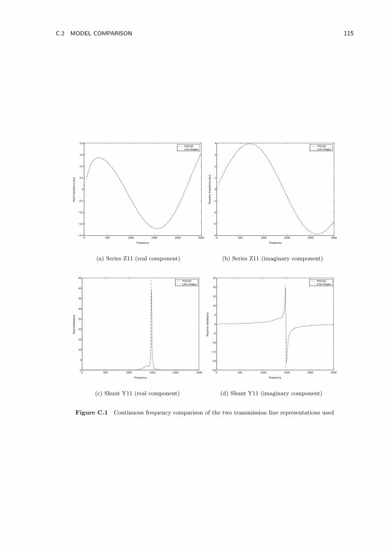
C.2 MODEL COMPARISON 115
0 500 1000 1500 2000 2500−0.4
−0.3
−0.2
−0.1
0
0.1
0.2
0.3
0.4
Rea
l Im
peda
nce
(pu)
Frequency
PSCADLine images
(a) Series Z11 (real component)
0 500 1000 1500 2000 2500−4
−3
−2
−1
0
1
2
3
4
Frequency
Rea
ctiv
e Im
peda
nce
(pu)
PSCADLine images
(b) Series Z11 (imaginary component)
0 500 1000 1500 2000 25000
5
10
15
20
25
30
35
40
45
Frequency
Rea
l Adm
ittan
ce
PSCADLine images
(c) Shunt Y11 (real component)
0 500 1000 1500 2000 2500−25
−20
−15
−10
−5
0
5
10
15
20
25
Frequency
Rea
ctiv
e A
dmitt
ance
PSCADLine images
(d) Shunt Y11 (imaginary component)
Figure C.1 Continuous frequency comparison of the two transmission line representations used
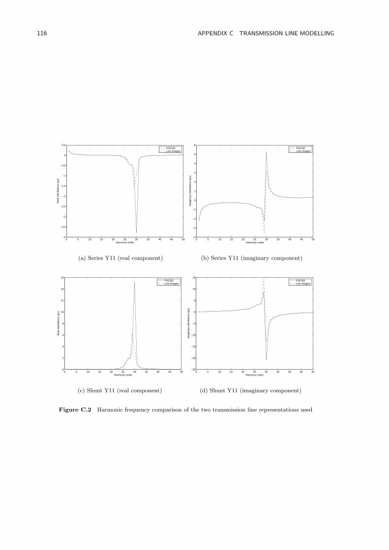
116 APPENDIX C TRANSMISSION LINE MODELLING
0 5 10 15 20 25 30 35 40 45 50−4
−3.5
−3
−2.5
−2
−1.5
−1
−0.5
0
0.5
Harmonic order
Rea
l Adm
ittan
ce (
pu)
PSCADLine Images
(a) Series Y11 (real component)
0 5 10 15 20 25 30 35 40 45 50−4
−3
−2
−1
0
1
2
3
4
5
6
Harmonic order
Imag
inar
y A
dmitt
ance
(pu
)
PSCADLine Images
(b) Series Y11 (imaginary component)
0 5 10 15 20 25 30 35 40 45 500
2
4
6
8
10
12
14
16
Harmonic order
Rea
l adm
ittan
ce (
pu)
PSCADLine Images
(c) Shunt Y11 (real component)
0 5 10 15 20 25 30 35 40 45 50−25
−20
−15
−10
−5
0
5
10
15
Harmonic order
Imag
inar
y ad
mitt
ance
(pu
)
PSCADLine Images
(d) Shunt Y11 (imaginary component)
Figure C.2 Harmonic frequency comparison of the two transmission line representations used
REFERENCES
[1] E.W. Kimbark. Direct Current Transmission. Wiley Interscience, New York, 1971.
[2] J. Arrillaga, C.P. Arnold, and B.J. Harker. Computer Modelling of Elecrical Power Systems.
John Wiley and Sons, 1983.
[3] N. Mohan, T.M. Undeland, and W.P. Robbins. Power Electronics:Converters, Applications,
and Design. John Wiley and Sons, 2nd ed., 1995.
[4] H.W. Dommel. Digital computer simulation of electromagnetic transients in single and mut-
liphase networks. IEEE Transactions on Power Apparatus and Systems, 88(4):388-399, Apr.
1969.
[5] D. Woodford, A. Gole, and R. Menzies. Digital simulation of dc links and ac machines. IEEE
Transactions on Power Apparatus and Systems, 102(6):1616-1623, Jun. 1983.
[6] T.J. Aprille and T.N. Trick. Steady-state analysis of non-linear circuits with periodic inputs.
Proceedings of the IEEE, 60(1):108-114, Jan. 1972.
[7] Manitoba HVdc Research Centre. PSCAD/EMTDC V3 users manual. Manitoba HVdc Re-
search Centre, Winnipeg, Canada, 1988.
[8] N. R. Watson. Frequency dependent ac system equivalents for harmonic studies and transient
converter simulation. PhD thesis, Department of Electrical and Electronic Engineering, Uni-
versity of Canterbury, Christchurch, New Zealand, 1987.
[9] R. Carbone, D. Menniti, R.E. Morrison, and A. Testa. Harmonic and interharmonic distor-
tion modeling in multiconverter systems. IEEE Transactions on Power Delivery, 10(3):1685-
1692, Jul. 1995.
[10] B.C. Smith. A harmonic domain model for the interaction of the HVdc converter with ac
and dc systems. PhD thesis, Department of Electrical and Electronic Engineering, University
of Canterbury, Christchurch, New Zealand, 1996.
[11] E. Acha. Modelling of power system transformers in the complex conjugate harmonic space.
PhD thesis, Department of Electrical and Electronic Engineering, University of Canterbury,
Christchurch, New Zealand, 1988.
118 REFERENCES
[12] A. Semlyen, E. Acha, and J. Arrillaga. Harmonic norton equivalent for the magnetising
branch of a transformer. IEE Proceedings, Part C, 143(2):162-169, Mar. 1987.
[13] W.H. Press, S.A. Teukolsky, W.T. Vetterling, and B.P. Flannery. Numerical Recipies in
FORTRAN. Cambridge University Press, 2nd ed., 1992.
[14] E.V. Larsen, D.H. Baker, and J.C. McIver. Low order harmonic interaction on ac/dc sys-
tems. IEEE Transactions on Power Delivery, 4(1):493-501, Jan. 1989.
[15] L. Hu and R. Yacamini. Harmonic transfer through convertors and hvdc links. IEEE Trans-
actions on Power Electronics, 7(3):514-525, Jul. 1992.
[16] D.L. Dickmander, S.Y. Lee, G.L. Desilets, and M. Granger. AC/DC harmonic interactions
in the presence of GIC for the Quebec-New England phase II HVdc transmission. IEEE
Transactions on Power Delivery, 9(1):68-78, Jan. 1994.
[17] A.R. Wood. An analysis of non-ideal HVdc converter behaviour in the frequency domain,
and a new control proposal. PhD thesis, Department of Electrical and Electronic Engineering,
University of Canterbury, Christchurch, New Zealand, 1993.
[18] D.J. Hume. Harmonic and interharmonic cross modulation in HVDC links. PhD thesis,
Department of Electrical and Computer Engineering, University of Canterbury, Christchurch,
New Zealand, 2002.
[19] M. Madrigal and E. Acha. Modelling of custom power equipment using harmonic domain
techniques. Proceedings of the 9th ICHQP, 1:264-269, 2000.
[20] C. Saniter, A.R. Wood, R. Hanitsch, and D. Schulz. Modelling the effects of AC system
impedance unbalance on PWM converters using frequency coupling matrices. Proceedings
Power Tech, IEEE Bologna, vol. 2, Jun. 2003.
[21] J. Reeve and J.A. Baron. Harmonic interaction between hvdc converters and ac power
systems. IEEE Transactions on Power Apparatus and Systems, 90(6)2785-2793, 1971.
[22] R. Yacamini and J.C. de Oliveira. Harmonics in multiple converter systems: a generalised
approach. IEE Proceedings Pt. B, 127:96-106, Mar. 1980.
[23] J.F. Eggleston. Harmonic modelling of transmission systems containing synchronus ma-
chines and static converters. PhD thesis, Department of Electrical and Electronic Engineer-
ing, University of Canterbury, Christchurch, New Zealand, 1985.
[24] C.D. Callaghan. Three phase integrated load and harmonic flows. PhD thesis, Department of
Electrical and Electronic Engineering, University of Canterbury, Christchurch, New Zealand,
1989.
REFERENCES 119
[25] R. Carbone, M. Fantauzzi, F. Gagliardi, and A. Testa. Some considerations on the iterative
harmonic analysis convergence. Proceedings of the 5th ICHQP, pp. 49-55, Sep. 1992.
[26] G. Carpinelli, F. Gagliardi, M. Russo, and D. Villacci. Generalised converter models for
iterative harmonic analysis in power systems. IEE Proceedings on Generation, Transmission
and Distribution, 141(5):445-451, Sep. 1994.
[27] G.T. Heydt and D. Xia. Harmonic power flow studies parts 1 and 2. IEEE Transactions on
Power Apparatus and Systems, 101(6):1257-1265, Jun. 1982.
[28] J.J. Rico, E. Acha, and T.J.E Miller. Harmonic domain modelling of three-phase thyristor-
controlled reactors by means of switching vectors and discrete convolutions. IEEE Transac-
tions on Power Delivery, 11(3):1678-1684, Jul. 1996.
[29] L.T.G. Lima, A. Semlyen, and M.R. Iravani. Harmonic domain periodic steady state model-
ing of power electronics apparatus: SVC and TCSC. IEEE Transactions on Power Delivery,
18(3):960-967, Jul. 2003.
[30] A. Medina and J. Arrillaga. Analysis of transformer-generator interaction in the harmonic
domain. IEE Proceedings on Generation, Transmission and Distribution, 141(1):38-46, May
1994.
[31] J. Arrillaga, A. Medina, M.L.V. Lisboa, M.A. Cavia, and P. Sanchez. The harmonic domain.
A frame of reference for power system harmonic analysis. IEEE Transactions on Power
Systems, 10(1):433-440, Feb. 1995.
[32] M.L.V. Lisboa. Three-phase three-limb transformer models in the Harmonic Domain. PhD
thesis, Department of Electrical and Electronic Engineering, University of Canterbury,
Christchurch, New Zealand, 1996.
[33] M. Valcarcel and J.G. Mayordomo. Harmonic power flow for unbalanced systems. IEEE
Transactions on Power Delivery, 8(4):2052-2059, Oct. 1993.
[34] G.N. Bathurst. A Newton solution for the harmonic analysis of power systems with mul-
tiple non-linear devices. PhD thesis, Department of Electrical and Electronic Engineering,
University of Canterbury, Christchurch, New Zealand, 1999.
[35] N.Q. Dinh, J. Arrillaga, and B.C. Smith. A steady-state model of direct connected
generator-HVdc converter units in the harmonic domain. IEE Proceedings on Generation,
Transmission and Distribution, 145(5):559-565, Oct. 1998.
[36] S.R. Sanders, M.J. Noworolski, X.Z. Liu, and G.C. Verghese. Generalized Averaging Method
for Power Conversion Circuits. IEEE Transactions on Power Electronics, 6(2):251-259, Apr.
1991.
120 REFERENCES
[37] A.M. Stankovic, P. Mattavelli, V. Caliskan, and G.C. Verghese. Modeling and Analysis of
FACTS Devices with Dynamic Phasors. IEEE Power Engineering Society Winter Meeting,
2:1440-1446, Jan. 2000.
[38] J.J. Rico, M. Madrigal, and E. Acha. Dynamic harmonic evolution using the extended
harmonic domain. IEEE Transactions on Power Delivery, 18(2):587-594, Arp. 2003.
[39] N.G. Hingorani. High Power Electronics and flexible AC Transmission System. IEEE Power
Engineering Review, pp. 3-4, Jul. 1988.
[40] N.G. Hingorani. Flexible AC transmission. IEEE Spectrum, 30:40-45, 1993.
[41] N.G. Hingorani, and L. Gyugyi. Understanding FACTS Concepts and Technology of Flexible
AC Transmission Systems. IEEE Press, New York, 1999.
[42] P. Petitclair, Y. Besanger, S. Bacha, and N. Hadjsaid. Facts modelling and control: Ap-
plications to the insertion of a STATCOM on power system. Proceedings of the 32nd IAS
Annual Meeting, Part 3,Oct. 1997.
[43] B.M.K. Han, G.G. Karady, J.K. Park, and S.I. Moon.Interaction analysis model for trans-
mission static compensator with EMTP. IEEE Transactions on Power Delivery, 13(4):1297-
1302, Oct. 1998.
[44] M.A. Madrigal, O. Anaya, E. Acha, J.G. Mayordomo, and R. Asensi. Single-phase PWM
converters array for three-phase reactive power compensation. I. Time domain studies. Pro-
ceedings of the 9th ICHQP, 2:541-547, 2000.
[45] C.K.L. Sao, P.W. Lenh, M.R. Iravani, and J.A. Martinez. A benchmark system for digital
time-domain simulation of a pulse-width-modulated D-STATCOM. IEEE Transactions on
Power Delivery, 17(4):1113-1120, Oct. 2002.
[46] O. Anaya-Lara and E. Acha. Modeling and analysis of custom power systems by
PSCAD/EMTDC. IEEE Transactions on Power Delivery, 17(1):266-272, Jan. 2002.
[47] W. Freitas and A. Morelato. A generalised current injection approach for modelling of facts
in power system dynamic simulation. Presented at 7th International Conference on AC-DC
Power Transmission, London, 2001.
[48] F.W. Huang, B.S. Rigby, and R.G. Harley. A static synchronous series compensator model
for EMTDC. Presented at 6th IEEE Africon Conference 2002, 2002.
[49] H.F. Wang. Modelling multiple FACTS devices into multi-machine power systems and ap-
plications. International Journal of Electrical Power & Energy Systems, 25:227-237, 2003.
[50] A.R. Wood, and C.M. Osauskas. A Linear Frequency-Domain Model of a STATCOM. IEEE
Transactions on Power Delivery, 19(3):1410-1418, Jul. 2004.
REFERENCES 121
[51] C.Saniter, R. Hanitsch, C. Osauskas, and H. Laird. A small signal frequency domain model
of a controlled PWM converter. Proceedings IEEE Postgraduate Power Conference, Bu-
dapest, 2002.
[52] G.N. Bathurst, N.R. Watson, and J. Arrillaga. Adaptive frequency-selection method for a
Newton solution of harmonics and interharmonics. IEE Proceedings on Generation, Trans-
mission and Distribution, 147(2):126-130, Mar. 2000.
[53] B.C. Smith, N.R. Watson, A.R. Wood, and J. Arrillaga. Steady state model of the AC/DC
converter in the harmonic domain. IEE Proceedings on Generation, Transmission and Dis-
tribution, 142(2):109-118, Mar. 1995.
[54] Z. Yang, C.Shen, M.L. Crow, and L. Zhang. An improved StatCom model for power flow
analysis. IEEE Power Engineering Society Summer Meeting, 2:1121-1126, Jul. 2000.
[55] W. Freitas, and A. Morelato. A generalised current injection approach for modelling of
FACTS in power system dynamic simulation. Seventh International Conference on AC-DC
Power Transmission, pp. 175-180, Nov. 2001.
[56] T.J. Densem. Three phase power system harmonic penetration. PhD thesis, Department of
Electrical and Electronic Engineering, University of Canterbury, Christchurch, New Zealand,
1983.
[57] J. Arrillaga, E. Acha, T.J. Densem, and P.S. Bodger. Ineffectiveness of Transmission Line
Transpositions at Harmonic Frequencies. IEE Proceedings, Part C, 133:99-104, Mar. 1986.
[58] J.R. Carson. Wave propagation in overhead wires with ground return. Bell System Technical
Journal, 5:539-54, 1926.
[59] C.A. Canizares. Power flow and transient stability models of FACTS controllers for voltage
and angle stability studies. IEEE Power Engineering Society Winter Meeting, 2:1447-1454,
2000.
[60] D.A. Woodford, A.M. Gole, and R.W. Menzies. Validation of digital simulation of hvdc
transients by field tests. IEE conf. publ. on AC and DC power transmission, (255):377-381,
1985
[61] L. Dong, M.L. Crow, Z. Yang, C. Shen, L. Zhang, and S. Atcitty. A reconfigurable FACTS
system for university laboratories. IEEE Transactions on Power Systems, 19:120-128, Feb.
2004.
[62] J. Arrillaga, D.A. Bradley, and P.S. Bodger. Power System Harmonics. John Wiley and
Sons, 1nd ed., 1985.
[63] E. Acha, C. Fuerte-Esquivel, H. Ambriz-Perez, and C. Angeles-Camacho. FACTS Modelling
and Simulation in Power Networks. John Wiley and Sons, 1st ed., 2004.