factors of multiple fatalities in car crashesanalytics.ncsu.edu/sesug/2016/sd-130_final_pdf.pdf ·...
TRANSCRIPT
PAPER SD-130
FACTORS OF MULTIPLE FATALITIES IN CAR CRASHES
BILL BENTLEY, VALUE-TRAIN; GINA COLAIANNI, KENNESAW STATE UNIVERSITY; KENNEDY ONZERE, KENNESAW STATE UNIVERSITY, CHERYL JONECKIS, US INTERNAL REVENUE SERVICE ADVISING PROFESSOR: XUELEI (SHERRY) NI, PH.D., KENNESAW STATE UNIVERSITY
1/15/2016
SESUG 2016
SESUG 2016 Paper SD-130 Project Report Page 1 of 6
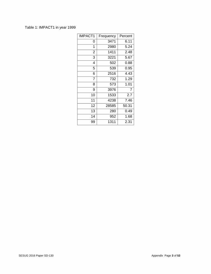
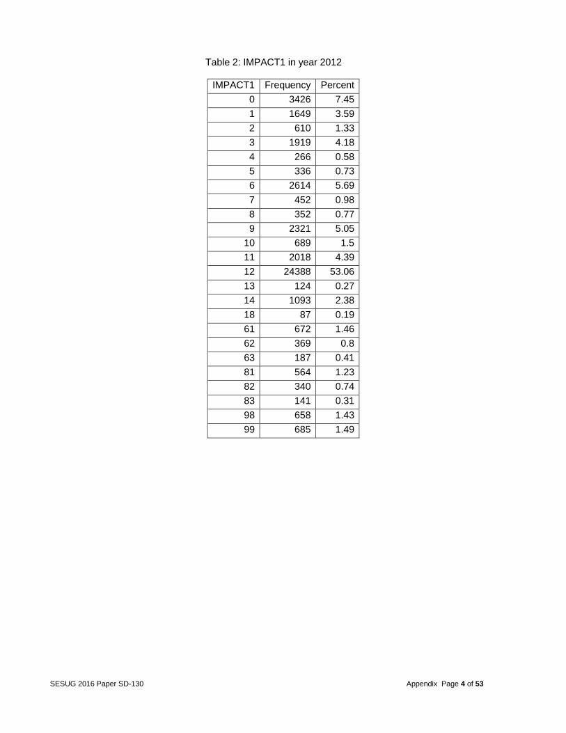
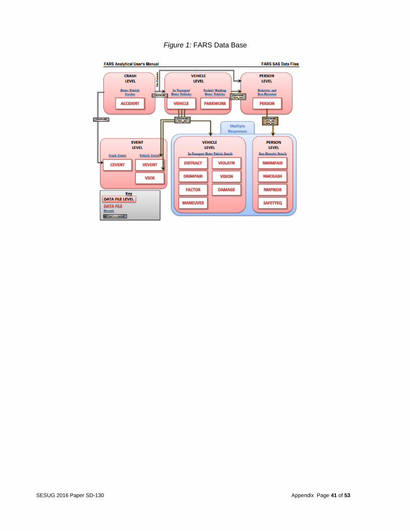
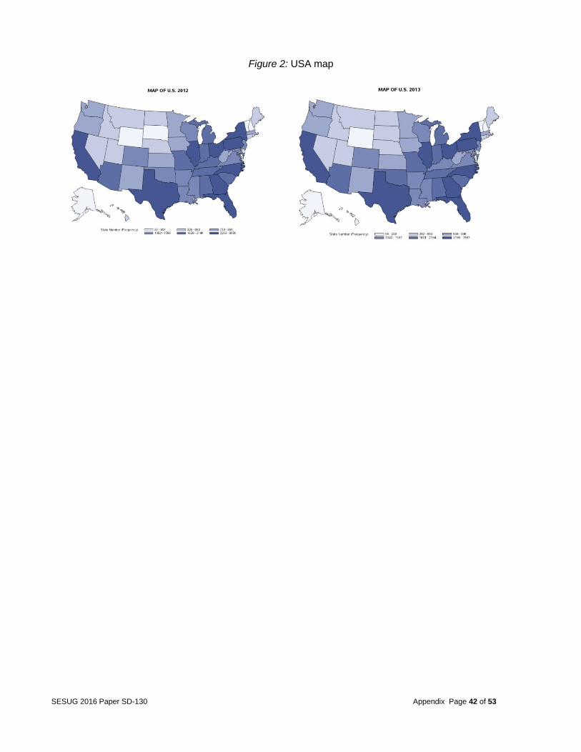
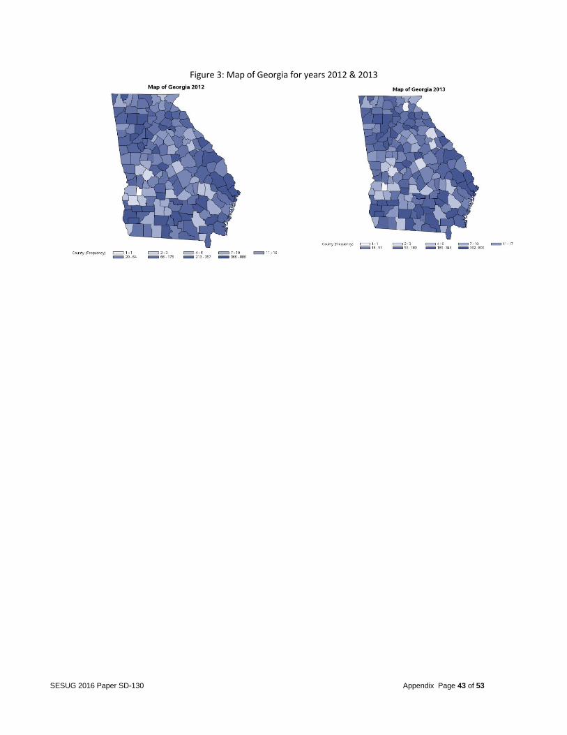
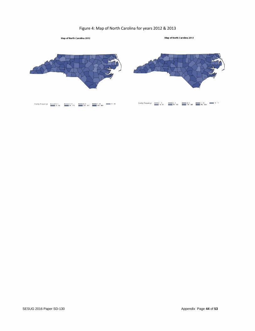
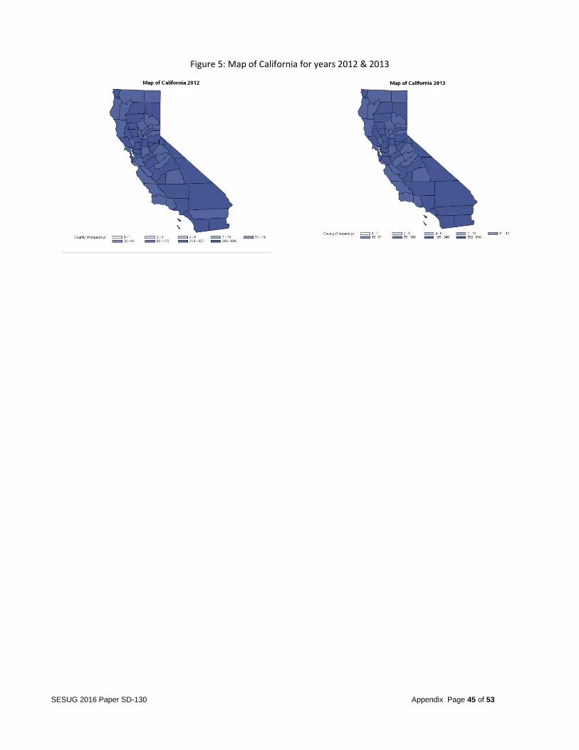
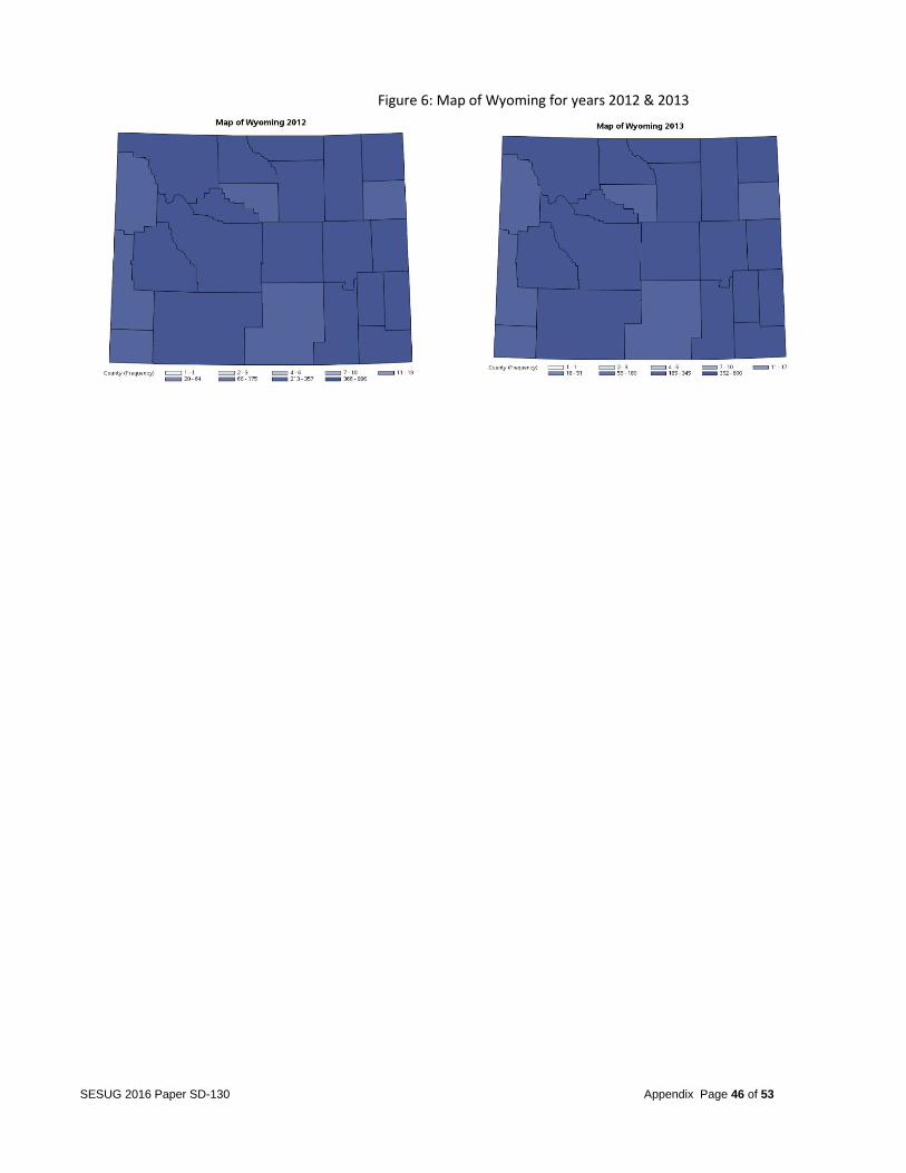
FACTORS OF MULTIPLE FATALITIES IN CAR CRASHES Introduction Road safety is a major concern for all United States of America citizens. According to the National Highway Traffic Safety Administration, 30,000 deaths are caused by automobile accidents annually. Oftentimes fatalities occur due to a number of factors such as driver carelessness, speed of operation, impairment due to alcohol or drugs, and road environment. Some studies suggest that car crashes are solely due to driver factors, while other studies suggest car crashes are due to a combination of roadway and driver factors. However, other factors not mentioned in previous studies may be contributing to automobile accident fatalities. The objective of this project was to identify the significant factors that lead to multiple fatalities in the event of a car crash. Data The FARS database the team was provided contained all fatal traffic crashes within the United States from 1999 to 2013. The 2012 database, for example, contained a total of 18 different files (see Figure 1 in the appendix for the file names and relations between the files). The ACCIDENT data file contained the characteristic and environment conditions at the time of the crash, with one record per accident. The VEHICLE data file contained information regarding each vehicle involved in the crash. The PERSON data file contained information describing each individual involved in the crash. The rest of the files included CEVENT, VEVENT, VSOE, FACTOR, VIOLATN, VISION, MANEUVER, DISTRACT, DRIMPAIR, NMIMPAIR, NMCRASH, NMPRIOR, SAFETYEQ, PARKWORK, and DAMAGE. These files included additional characteristics of the crash and contained multiple records per vehicle or person. The team focused on the years 2012 and 2013 because they were the most recent records, and the databases and variables were consistent for those 2 years. Over time, numerous databases were created, and several variables changed either in formats or in values. For example, the variable IMPACT1 had categories added and deleted over time and changed meanings several times. Tables 1 and 2 (in the appendix) compare the different categories between the years 1999 and 2012. The year 2012 was used as the training data and year 2013 was used as the testing data. Therefore, one should be able to see whether a big change occurs in the relationship after year 2012. Since no change occurred between the years, the current year data can be used to predict the next year’s fatalities or to make new recommendations. If significant changes over the years had occurred, a time series-based model could have been adopted to investigate the seasonality, trends, and change points. A quick insight into the data revealed that the frequency of accidents by state shown in Figure 2 (in the appendix) does not change significantly between the years. For example, the states Georgia and California both contained the highest number of accidents. The team randomly selected states to check the frequency counts in details. The states included Georgia, North Carolina, California, and Wyoming (as shown in Figures 3 through 6 in the appendix). Problem The project goal was to examine the number of deaths in a single accident and the contributing factors strongly related to accidents with multiple fatalities. The team’s recommendations will aim at reducing the number of accidents that potentially lead to multiple fatalities. Only the first event in the sequence of events in a multiple events accident was used, for once the accident sequence started, little action could be taken to prevent the subsequent sequence of events
SESUG 2016 Paper SD-130 Project Report Page 2 of 6
(based on the available data). This, plus a careful inspection of what each database contained and what each variable represented, gave a basis of making the data preparation decisions described next. Data Cleaning/Validation In preparation for data analysis, the following actions were taken: 1. The team chose to use 2012 datasets as the training sets and 2013 data for validation
purposes. The reasons for this decision were explained in the previous section. 2. The CEVENT and VEVENT databases were streamlined to include only those records
pertaining to event number one. The team decided to take only event one due to the fact that little action could be taken to prevent the subsequent sequence of events.
3. The VSOE database was not used because it was a subset of the VEVENT database. 4. An analysis of the databases with multiple responses was completed. For the vehicle level
databases, the team found the duplications were due to the multiple descriptions for the same vehicle from different angles. Therefore, the deduplication was done so that only one record per vehicle was available which created additional variables based on the categories. The following vehicle level files were transformed: DAMAGE and DRIMPAIR. Similar duplications were found in the person level files. The deduplication was processed as well in order for only one record to be available per person. The person level files included NMCRASH, NMIMPAIR, NMPRIOR, and SAFETYEQ.
5. Additional databases that included multiple responses were condensed by the number of
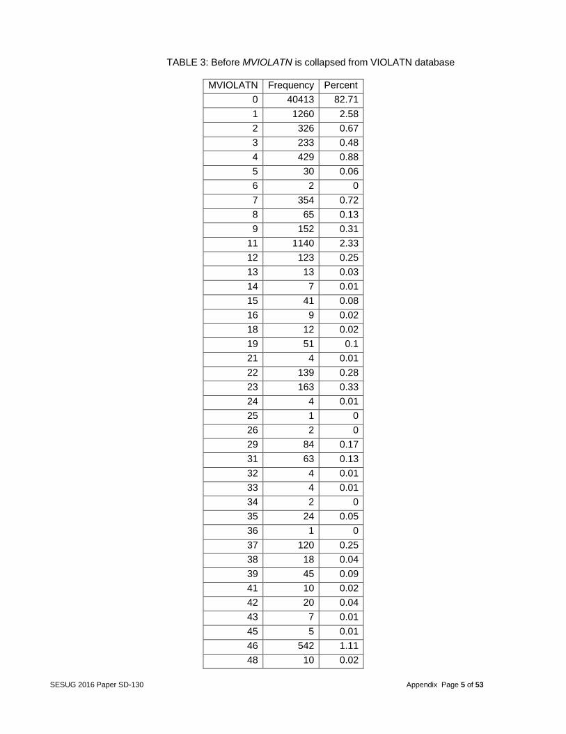
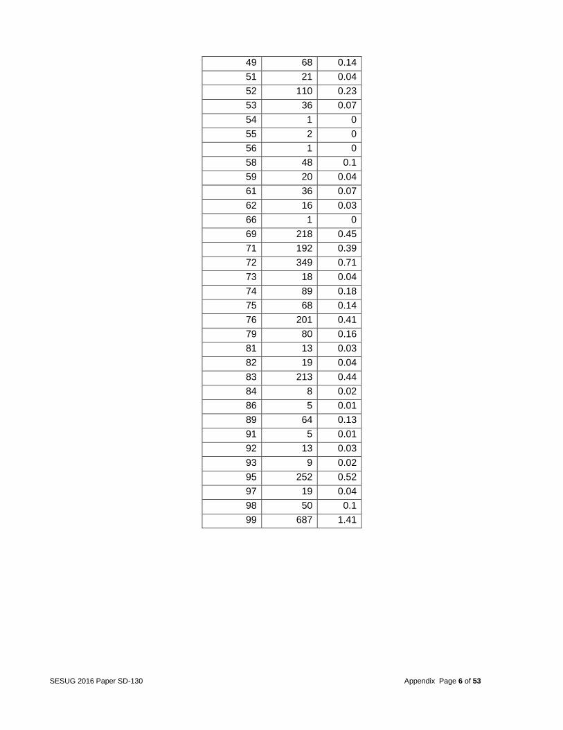
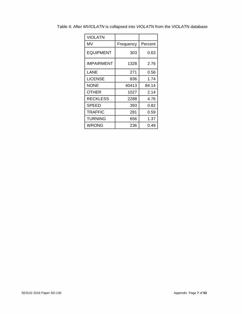
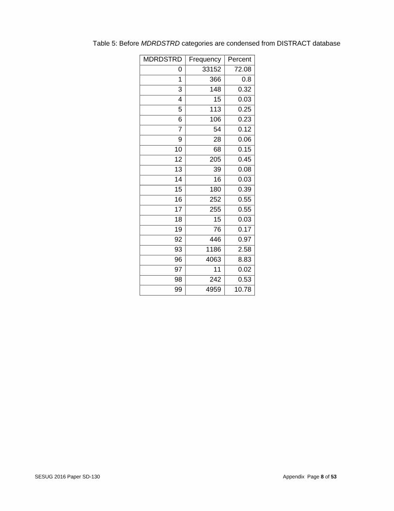
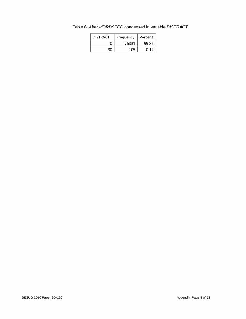
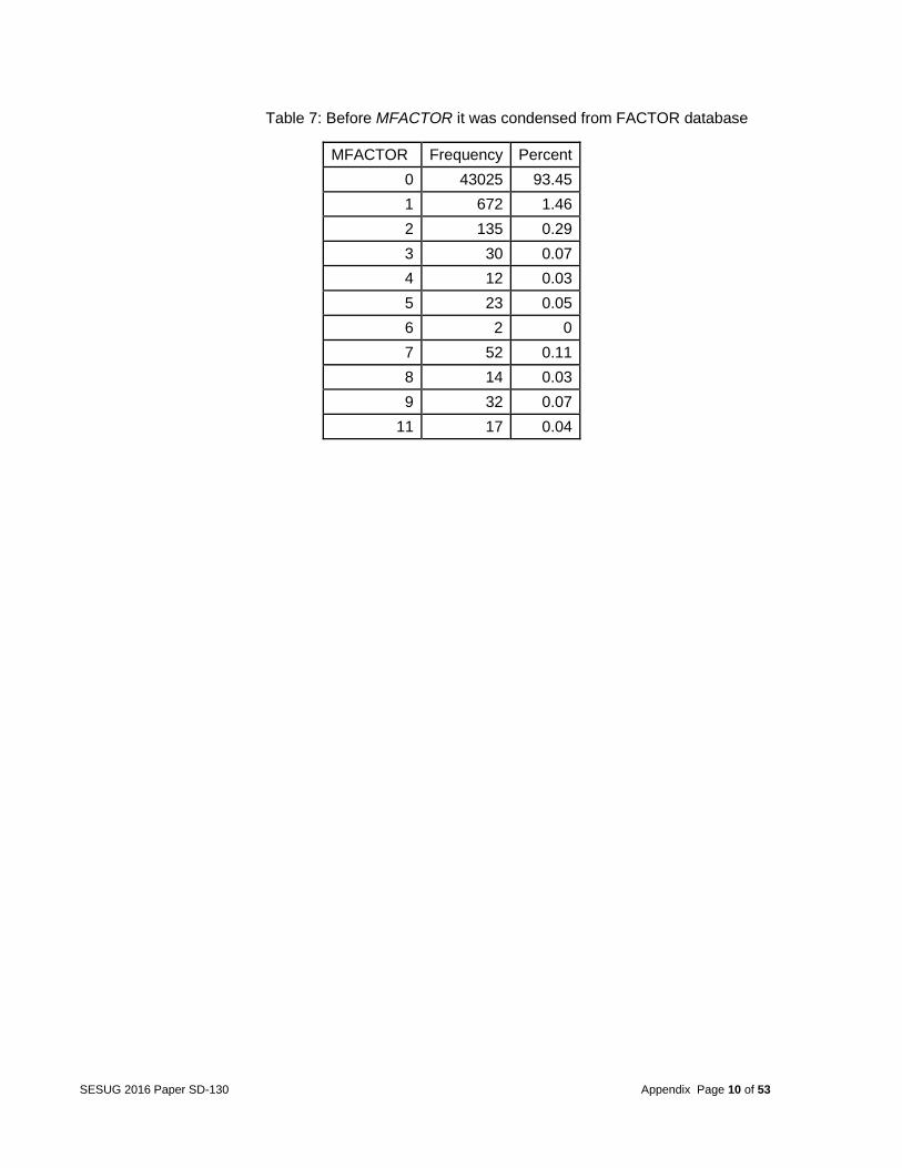
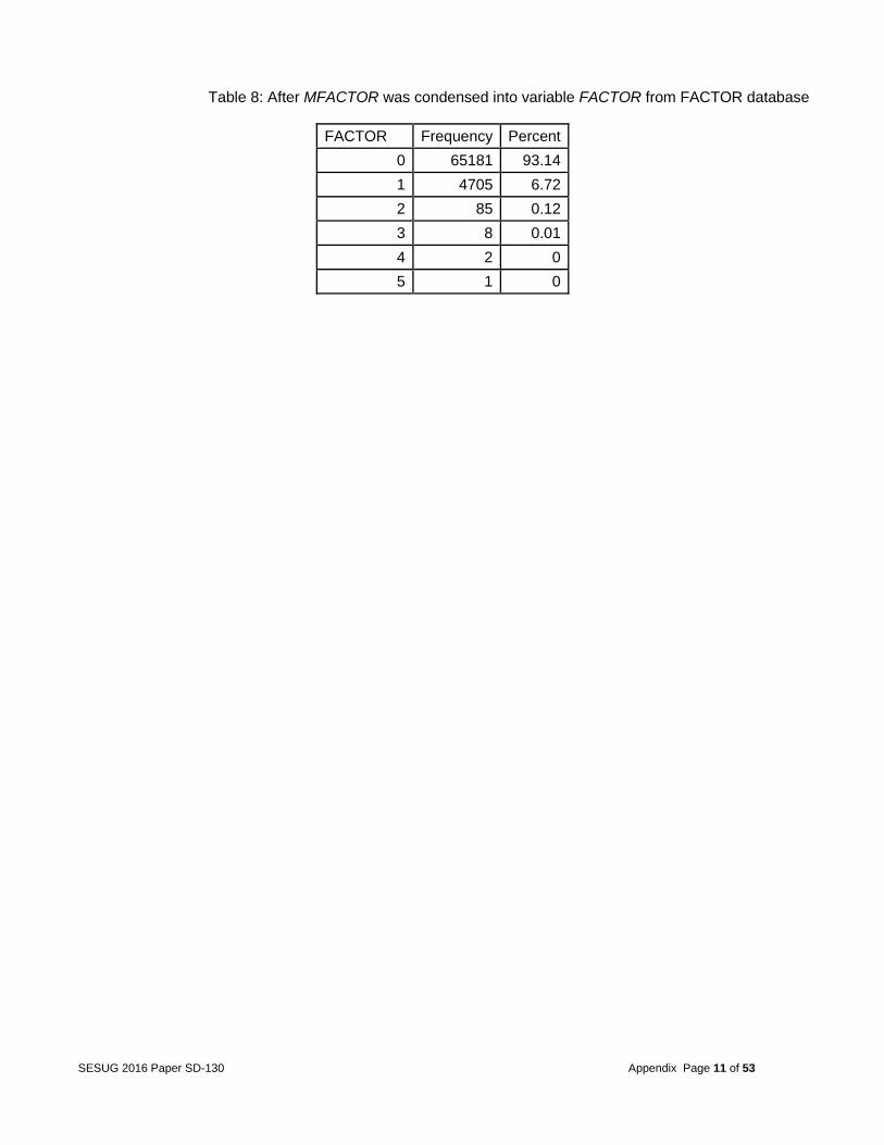
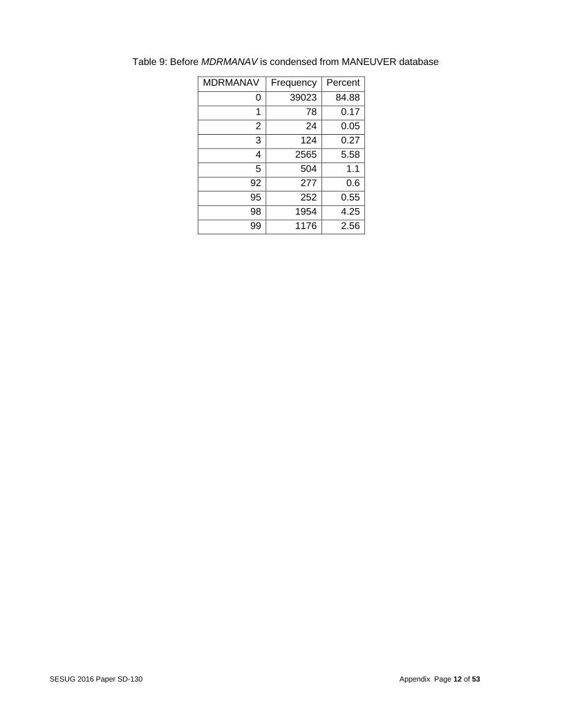
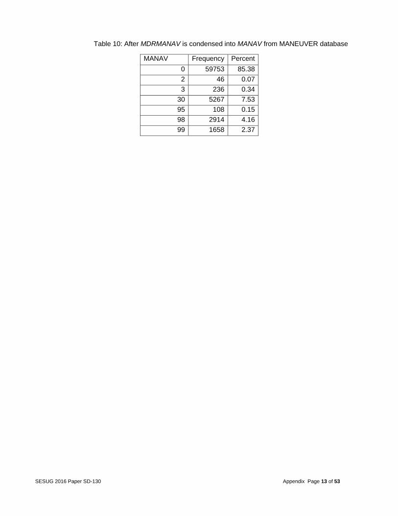
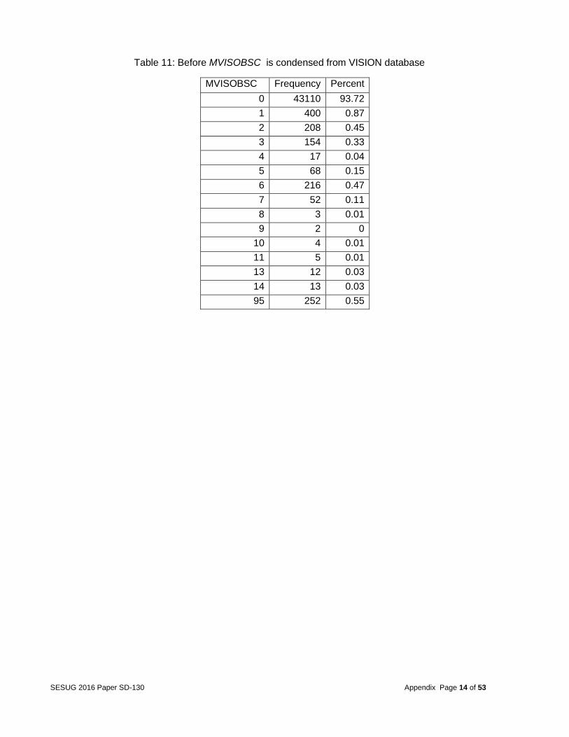
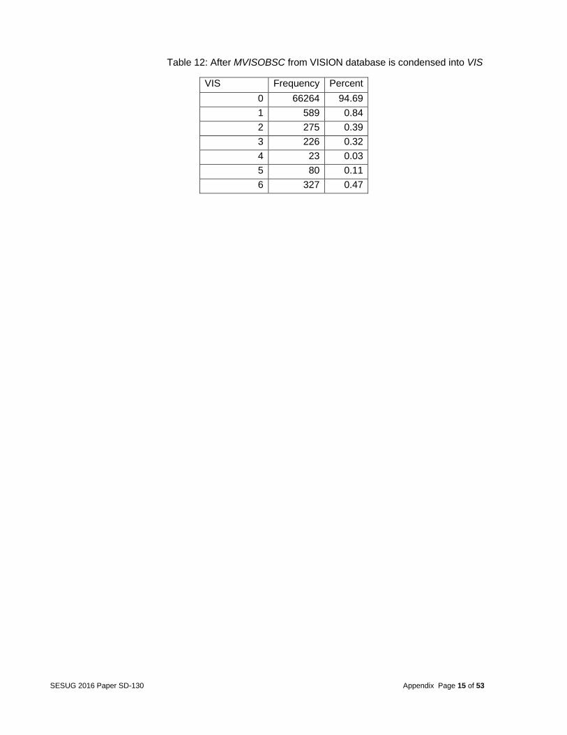
different categories. For example, the variable MVIOLATN from the database VIOLATN identified all violations charged to the driver. Due to the fact that there were several drivers with multiple violations, the team decided to collapse similar categories. The variable MVIOLATN was collapsed from 99 categories to 11. As a result, only one record per vehicle for the violation codes occurred. More details are given in the appendix in Tables 3 and 4. Other variables included MDRDSTRD in the DISTRACT database. This variable was condensed from 26 categories to 2 based on whether the vehicle had multiple distractions or not (as shown in Tables 5 and 6 in appendix). The variable MFACTOR in the FACTOR database was condensed from 21 categories to 2 by summing up the total number of factors per vehicle (as shown in Tables 7 and 8 in the appendix). The variable MDRMANAV in the MANEUVER database was condensed from 10 categories to seven (as shown in Tables 9 and 10 in the appendix), and VISION was condensed from 19 categories to 14 (as shown in Tables 11 and 12 in the appendix).
6. For the PARKWORK dataset, only the records associated with event number 1 were kept. 7. By simple descriptive statistical analysis, no influential points such as outliers were found in
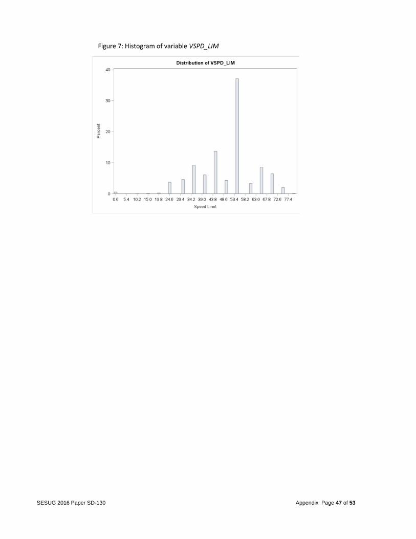
the data bases. The missing values were replaced with the median for each numeric variable because most of the distributions were skewed. A histogram of the variable VSPD_LIM is shown in the appendix as an example (Figure 7).
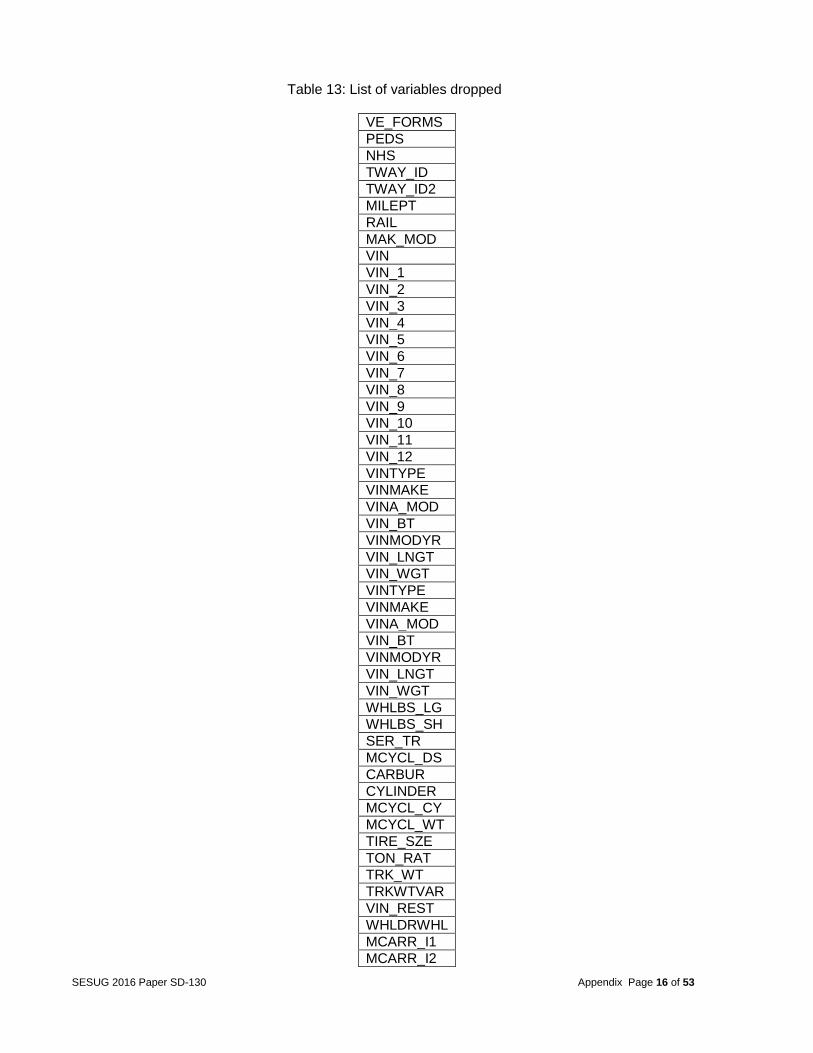
8. A careful inspection of each variable’s description was done. Identification variables, such as
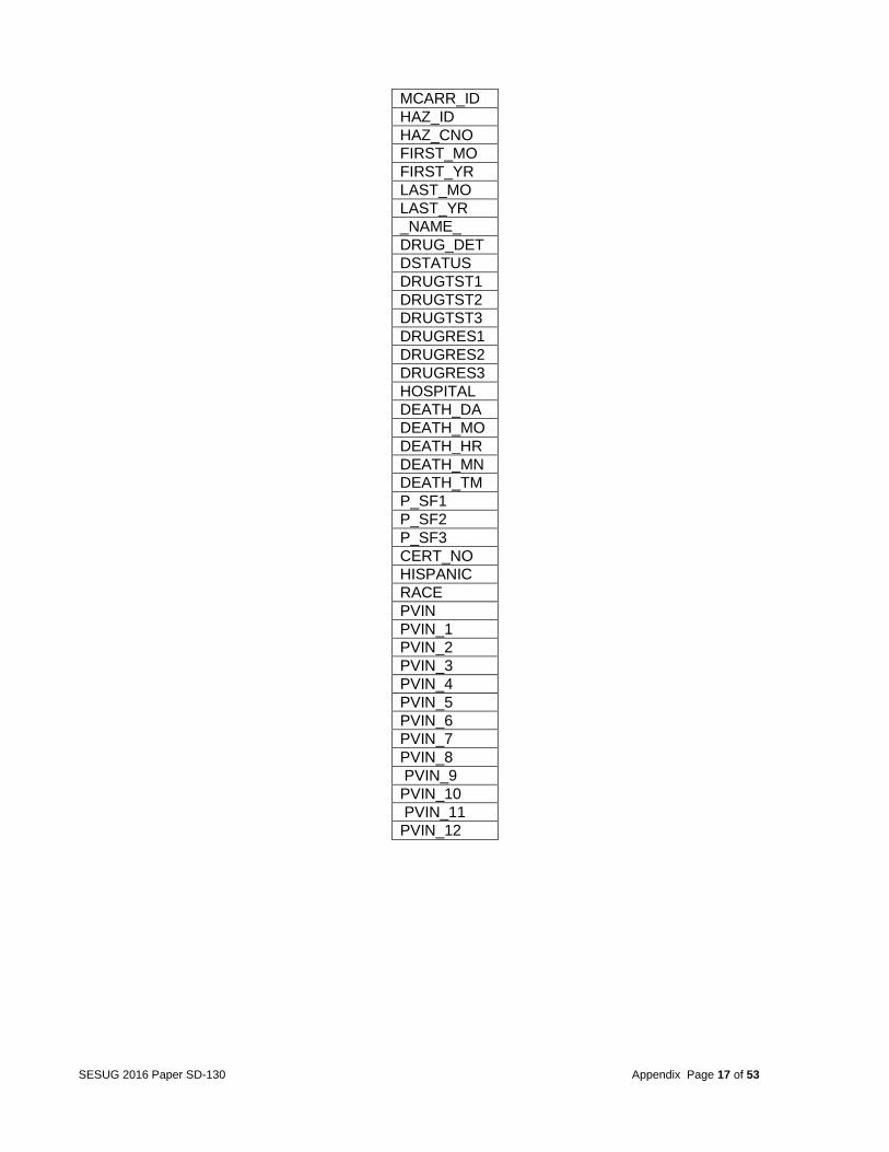
VIN number and variables that did not meet the team’s goal were dropped. See the completed list in the appendix (table 13).
SESUG 2016 Paper SD-130 Project Report Page 3 of 6
9. The various databases were merged together into person level, so each record was a person. Note that there could be multiple people in a vehicle and multiple vehicles in an accident. The merged data may have duplicated information for the same accident and same vehicle. The team decided to do so to keep the most detailed information in an accident. The order of merging was as follows:
a. CEVENT into ACCIDENT by case number b. VEVENT into VEHICLE by case number and vehicle number c. All vehicle level databases into VEHICLE by case number and vehicle number and
finally that resulting database into the PERSON database by case number and vehicle number.
d. The final database for analysis contained 76436 records and 239 variables, the same number of records in the person database.
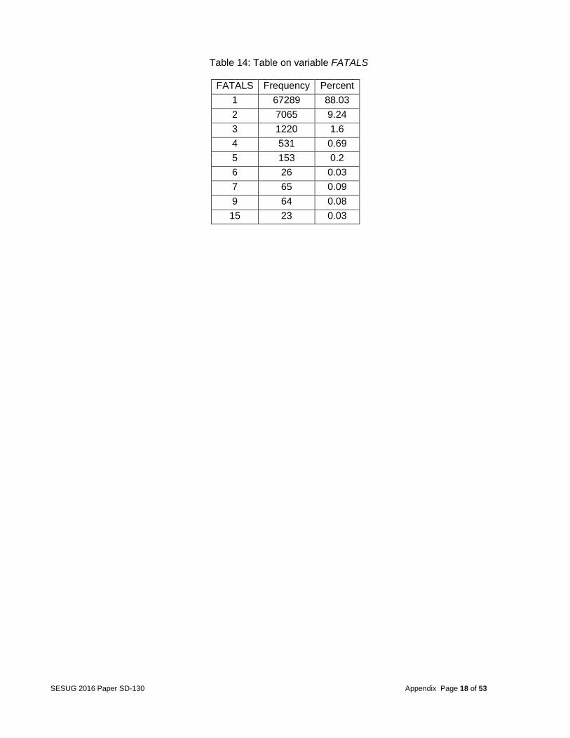
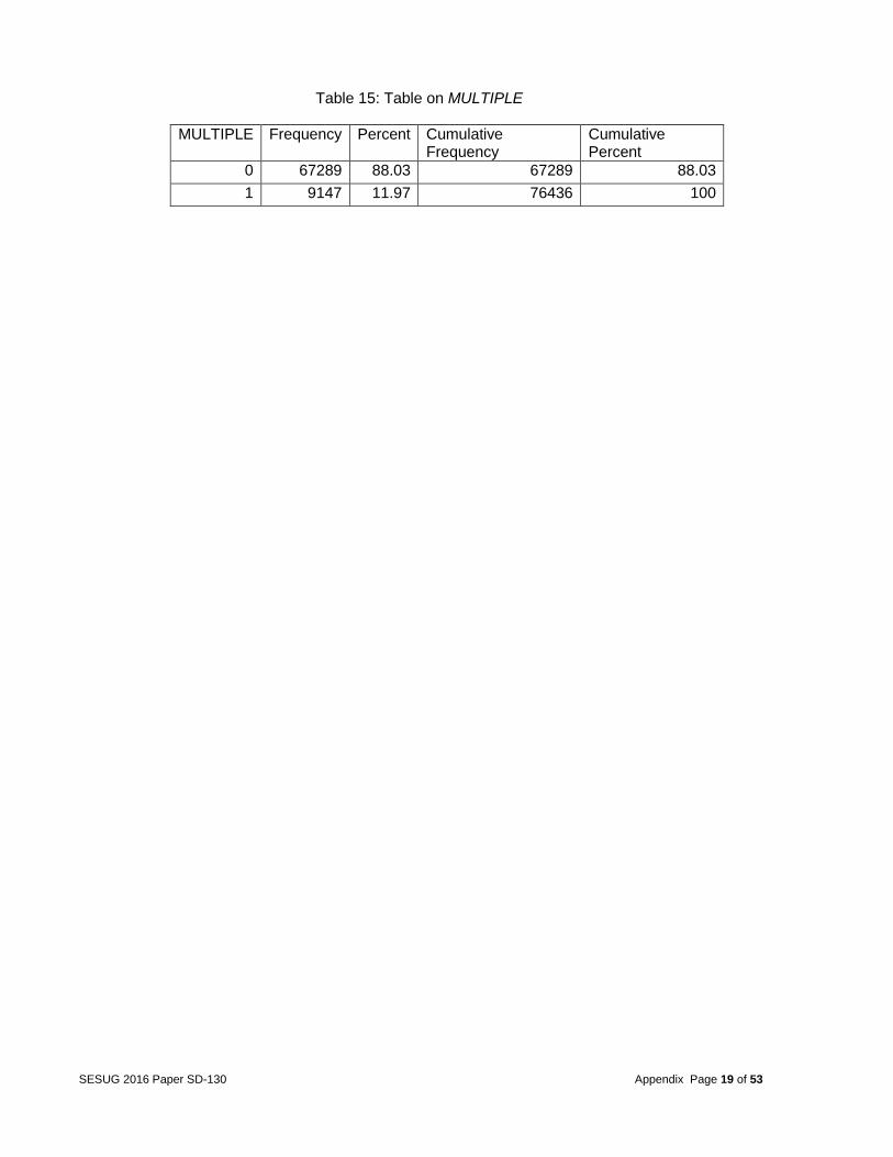
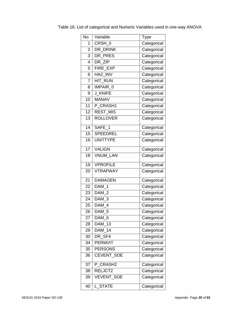
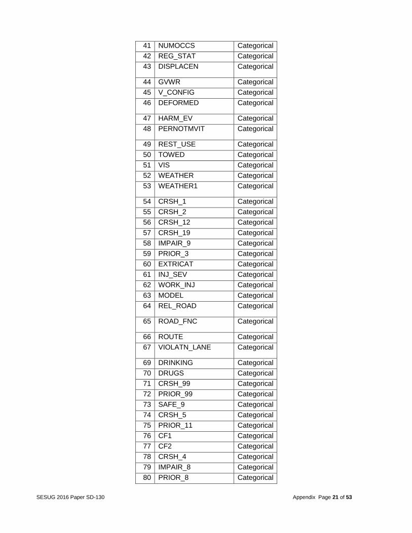
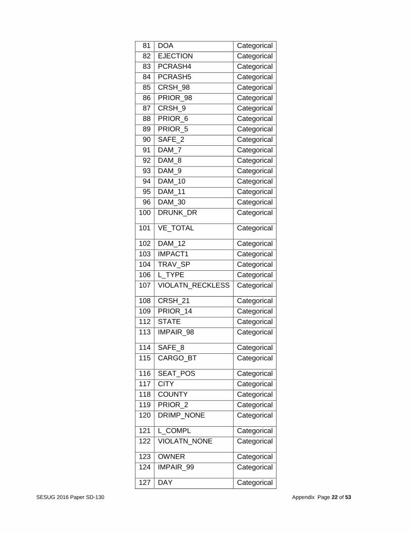
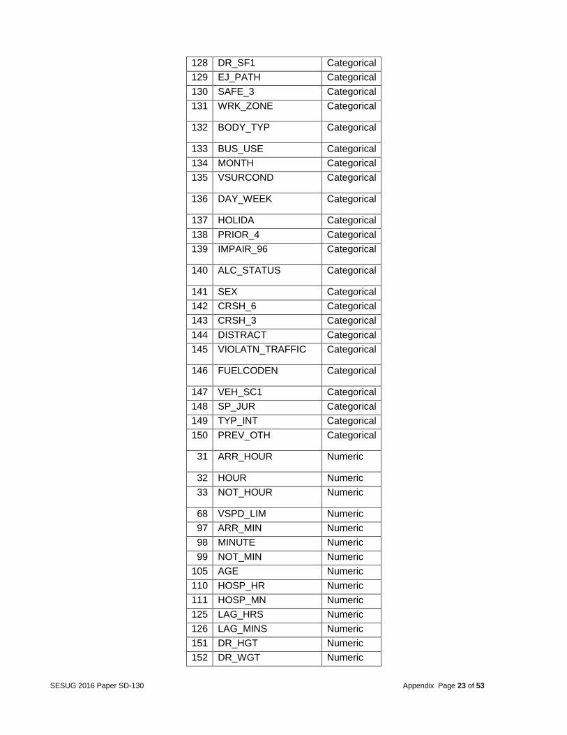
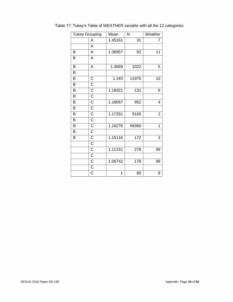
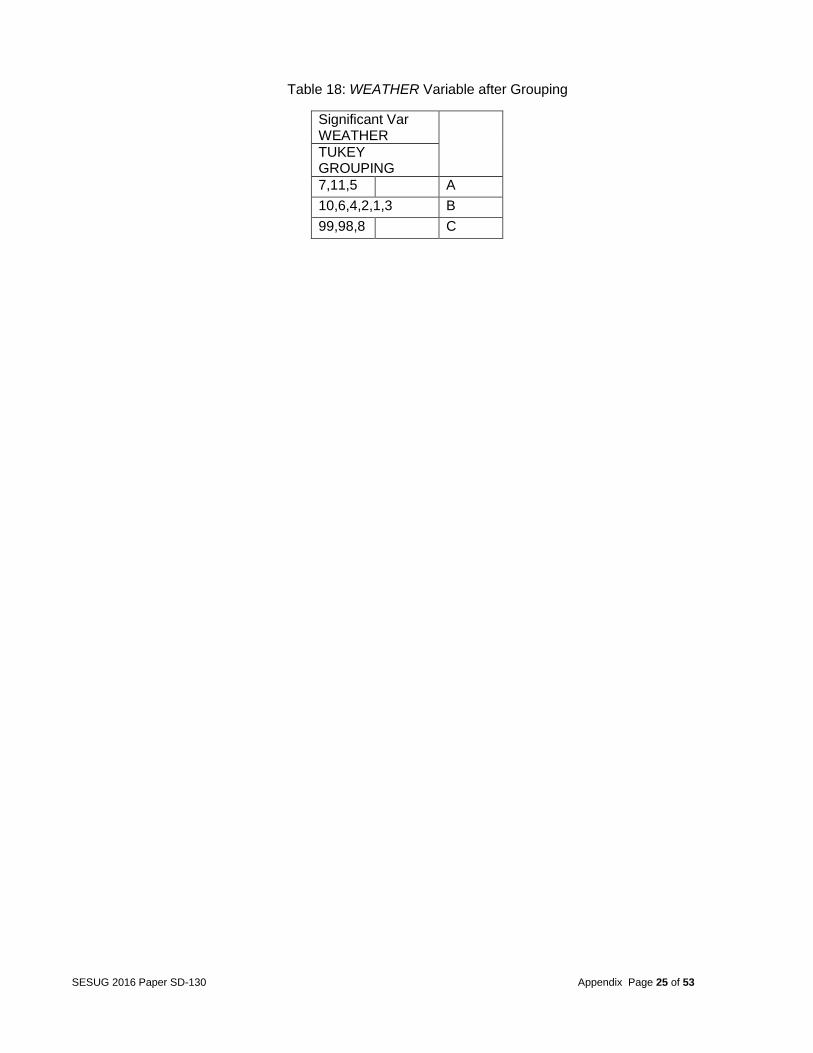
After the final dataset was created, the response variable was analyzed. The goal of this analysis was to determine what factors caused multiple deaths, so the team focused on the target variable FATALS. This variable identified the number of fatally injured persons in a crash. The frequency table of the variable FATALS is shown in appendix (Table 14). From this variable, a binary categorical variable was created to run a logistic regression model. This variable called MULTIPLE was used with 1 equal to multiple deaths and 0 equal to a single death. The frequency table of MULTIPLE is shown in appendix (table 15). Analysis After merging the datasets, the next step was to determine which variables were statistically related with fatalities in automobile accidents. The team identified these variables in 3 steps: Step 1 -- Relation between one predictor and the target based on one-way ANOVA or Pearson Correlation The team first identified the potential significant factors through a one-by-one checking. Only the variables with the p-value less than 0.05 were kept. As a result, 152 predictors were strongly related with the target variable, when no other factors were considered. 84 variables were not significant and were discarded from further consideration. Among the 152 significant variables, 14 were quantitative and 138 are categorical (full list in Table 16 in the appendix). Many of the categorical variables had too many categories, which would increase the complexity of the models and make the explanation too difficult in the later analysis stage. Therefore, Tukey’s post-hoc tests were applied to combine the categories with no significant difference. For example, the variable WEATHER (describing the atmospheric conditions that existed at the time of crash) initially had 12 categories but Tukey’s grouping suggested condensing these categories to 3 (see Table 17 & 18 in the appendix). Step 2 -- Variable clustering to reduce the collinearity among the predictors The above selected variables may have overlapped redundant information. For example, variable VSPD_LIM (speed limit just prior to vehicle’s critical pre-crash) and variable INJ_SEV (severity of injury) are highly correlated. They measure the similar characters in the accident (of a vehicle or of a person). When redundant variables are included in some of the model building procedures, the parameter estimates can become unstable and create a confounded interpretation. Therefore, deciding on the correct relationships between dependent and independent variables becomes difficult if multicollinearity is strong. In fact, given the nature of the datasets for this project,
SESUG 2016 Paper SD-130 Project Report Page 4 of 6
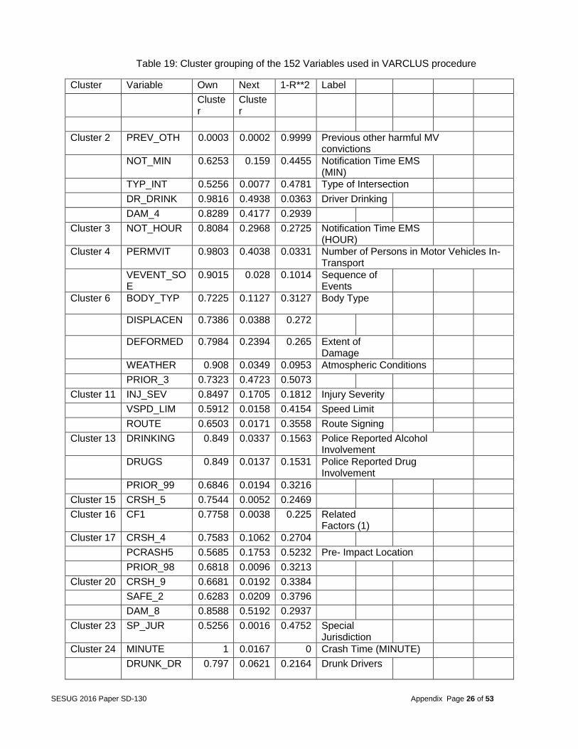
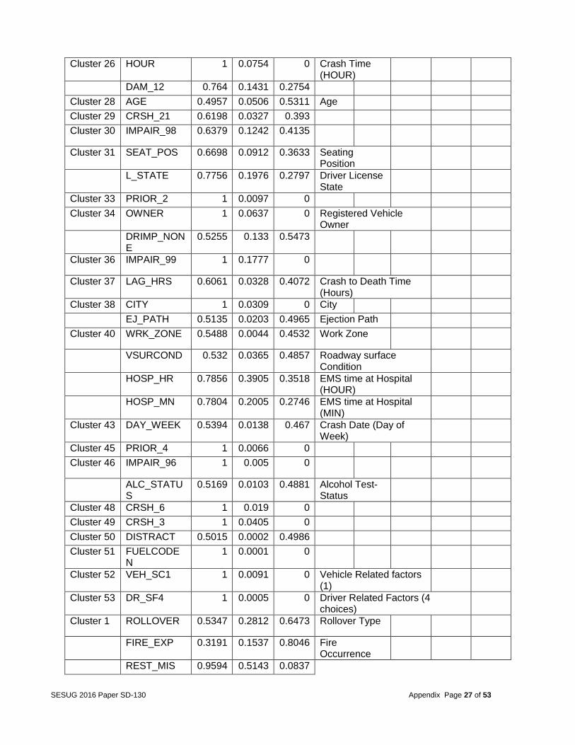
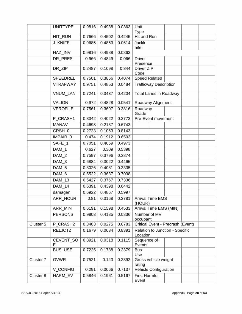
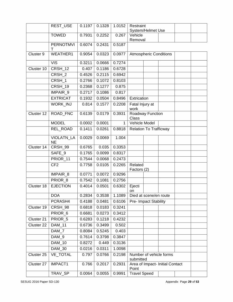
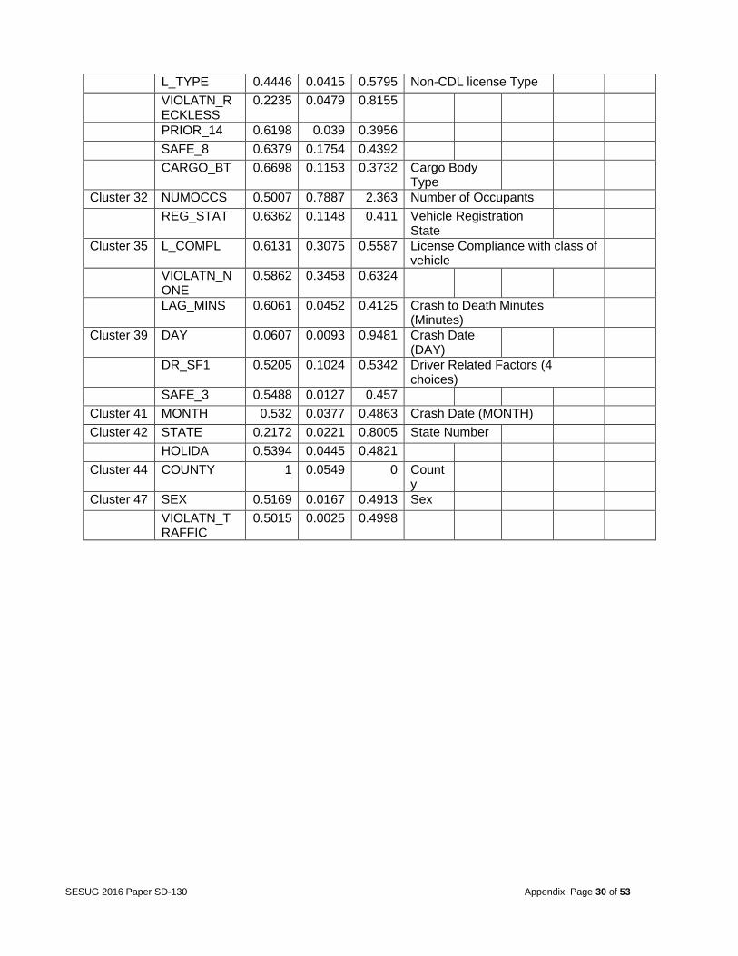
multicollinearity could be an issue to cause biased results. In order to reduce its effect, predictor variables were grouped into clusters, and representative variables selected from each cluster. The PROC VARCLUS procedure was used to do variable clustering based on the maximum eigenvalue threshold. The VARCLUS procedure only performs the clustering for numerical variables. Most of our variables were categorical. In order to do the grouping, the team changed the categorical coding into the mean of the target variable (FATALS, number of deaths) in that specific category. Note that this transformation will keep the category differences and also save the relation between the categorical factor and the target. This transformation was only used in this stage. In the later modelling stage, the team used the original categorical coding. As a result, there were 53 clusters (Table 19 of the Appendix). Variables in the same cluster were similar to each other, and variables in different clusters were different from each other. Representative variables from each cluster were then identified. Since the variables selected should have a high correlation with their respective cluster and low correlation with other clusters, 1 – R2 ratio was used to select the variables to be used for modelling. The variables with the lowest 1 - R2
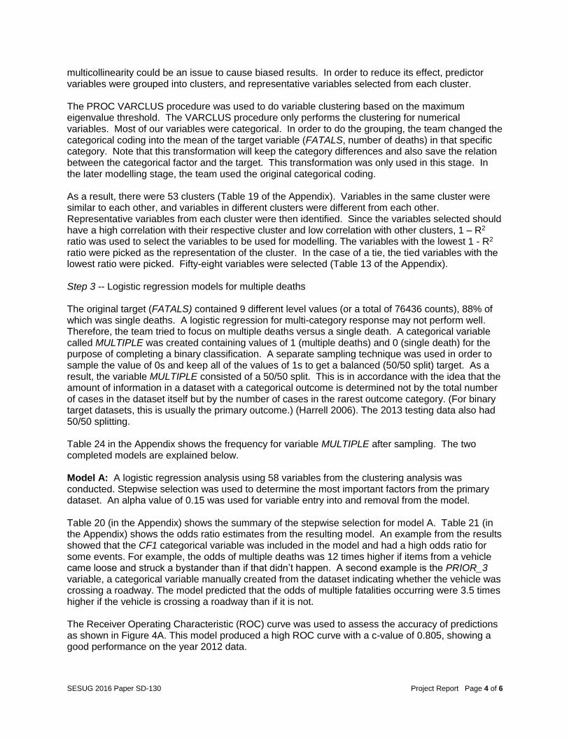
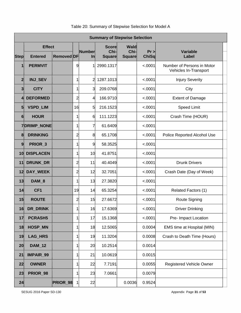
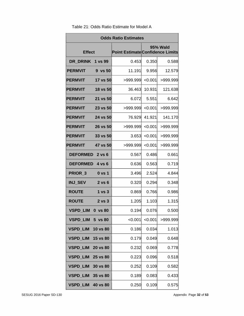
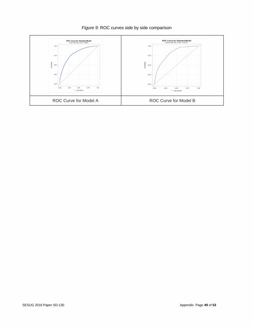
ratio were picked as the representation of the cluster. In the case of a tie, the tied variables with the lowest ratio were picked. Fifty-eight variables were selected (Table 13 of the Appendix). Step 3 -- Logistic regression models for multiple deaths The original target (FATALS) contained 9 different level values (or a total of 76436 counts), 88% of which was single deaths. A logistic regression for multi-category response may not perform well. Therefore, the team tried to focus on multiple deaths versus a single death. A categorical variable called MULTIPLE was created containing values of 1 (multiple deaths) and 0 (single death) for the purpose of completing a binary classification. A separate sampling technique was used in order to sample the value of 0s and keep all of the values of 1s to get a balanced (50/50 split) target. As a result, the variable MULTIPLE consisted of a 50/50 split. This is in accordance with the idea that the amount of information in a dataset with a categorical outcome is determined not by the total number of cases in the dataset itself but by the number of cases in the rarest outcome category. (For binary target datasets, this is usually the primary outcome.) (Harrell 2006). The 2013 testing data also had 50/50 splitting. Table 24 in the Appendix shows the frequency for variable MULTIPLE after sampling. The two completed models are explained below. Model A: A logistic regression analysis using 58 variables from the clustering analysis was conducted. Stepwise selection was used to determine the most important factors from the primary dataset. An alpha value of 0.15 was used for variable entry into and removal from the model. Table 20 (in the Appendix) shows the summary of the stepwise selection for model A. Table 21 (in the Appendix) shows the odds ratio estimates from the resulting model. An example from the results showed that the CF1 categorical variable was included in the model and had a high odds ratio for some events. For example, the odds of multiple deaths was 12 times higher if items from a vehicle came loose and struck a bystander than if that didn’t happen. A second example is the PRIOR_3 variable, a categorical variable manually created from the dataset indicating whether the vehicle was crossing a roadway. The model predicted that the odds of multiple fatalities occurring were 3.5 times higher if the vehicle is crossing a roadway than if it is not. The Receiver Operating Characteristic (ROC) curve was used to assess the accuracy of predictions as shown in Figure 4A. This model produced a high ROC curve with a c-value of 0.805, showing a good performance on the year 2012 data.
SESUG 2016 Paper SD-130 Project Report Page 5 of 6
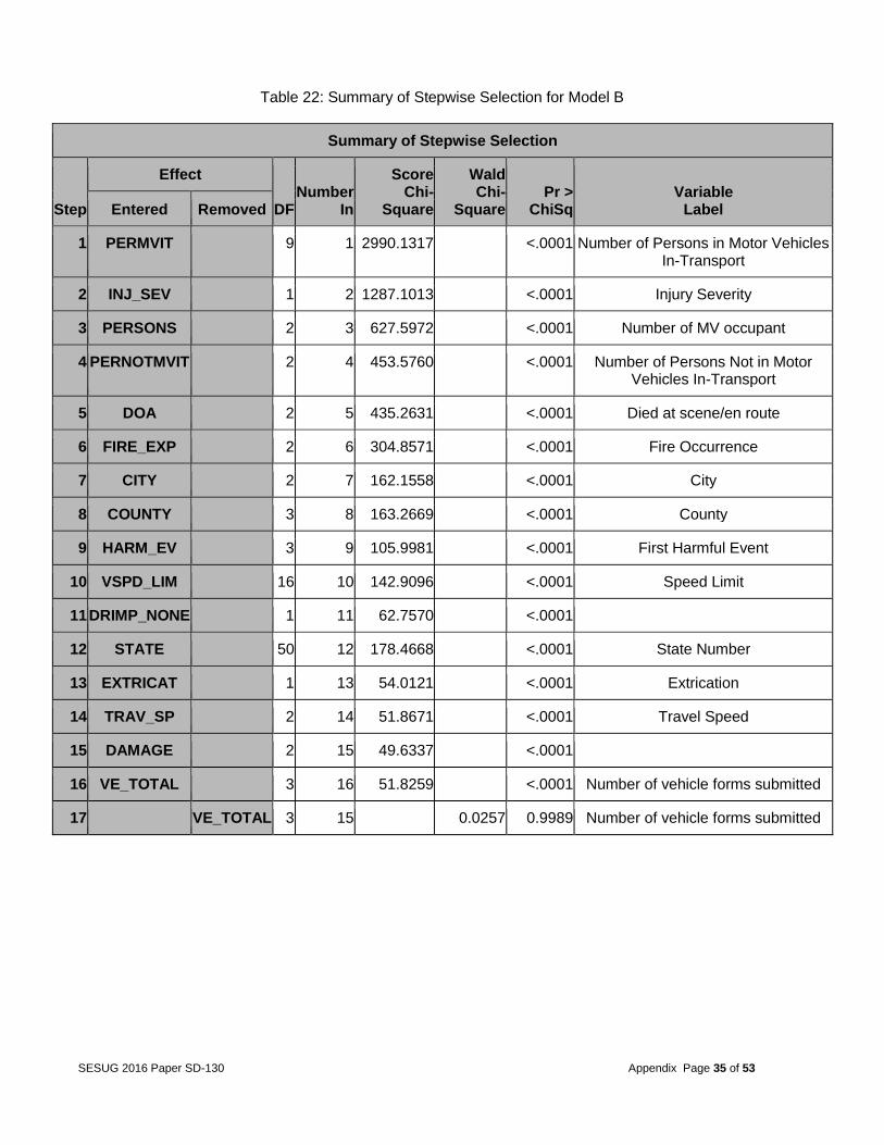
Model B: A logistic regression analysis and stepwise selection procedure was conducted using the same technique for model A but with all of the 152 variables in the dataset. Therefore, the selected variables may have a multicollinearity issue. This model was built to see if we ignored multicollinearity, whether a stronger model will be possible because the existence of multicollinearity does not affect the prediction of the target variable. So if the goal of a model user is to make accurate predictions about the likely occurrence of a fatal crash that results in multiple deaths, this model may be preferred. Table 22 shows the summary of the stepwise selection. Table 23 show the odds ratio estimates. An example of the model results for variable DOA is that based on the odds ratio estimate, the odds of multiple deaths are 2.3 times higher if someone died at the crash scene compared to no deaths at the crash scene. This variable is in a variable cluster containing three other variables. They are PCRASH4 (vehicle skidding, etc.), PCRASH5 (vehicle departed lane or roadway etc.) and EJECTION (people ejected from vehicle). These variables did not end up in this model but they are likely to affect the severity of the accident so they may have diluted the reported effects of the DOA variable because of collinearity. The ROC curve (Figure 9) was used to assess the accuracy of predictions. This model did produce a high ROC curve with a c-value of 0.8144.
SESUG 2016 Paper SD-130 Project Report Page 6 of 6
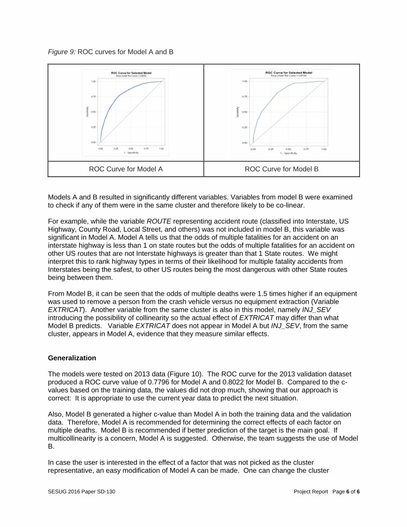
Figure 9: ROC curves for Model A and B
ROC Curve for Model A ROC Curve for Model B
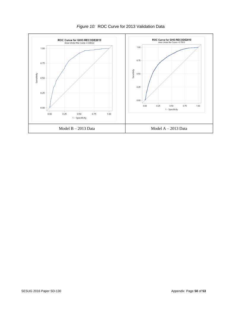
Models A and B resulted in significantly different variables. Variables from model B were examined to check if any of them were in the same cluster and therefore likely to be co-linear. For example, while the variable ROUTE representing accident route (classified into Interstate, US Highway, County Road, Local Street, and others) was not included in model B, this variable was significant in Model A. Model A tells us that the odds of multiple fatalities for an accident on an interstate highway is less than 1 on state routes but the odds of multiple fatalities for an accident on other US routes that are not Interstate highways is greater than that 1 State routes. We might interpret this to rank highway types in terms of their likelihood for multiple fatality accidents from Interstates being the safest, to other US routes being the most dangerous with other State routes being between them. From Model B, it can be seen that the odds of multiple deaths were 1.5 times higher if an equipment was used to remove a person from the crash vehicle versus no equipment extraction (Variable EXTRICAT). Another variable from the same cluster is also in this model, namely INJ_SEV introducing the possibility of collinearity so the actual effect of EXTRICAT may differ than what Model B predicts. Variable EXTRICAT does not appear in Model A but INJ_SEV, from the same cluster, appears in Model A, evidence that they measure similar effects. Generalization The models were tested on 2013 data (Figure 10). The ROC curve for the 2013 validation dataset produced a ROC curve value of 0.7796 for Model A and 0.8022 for Model B. Compared to the c-values based on the training data, the values did not drop much, showing that our approach is correct: It is appropriate to use the current year data to predict the next situation. Also, Model B generated a higher c-value than Model A in both the training data and the validation data. Therefore, Model A is recommended for determining the correct effects of each factor on multiple deaths. Model B is recommended if better prediction of the target is the main goal. If multicollinearity is a concern, Model A is suggested. Otherwise, the team suggests the use of Model B. In case the user is interested in the effect of a factor that was not picked as the cluster representative, an easy modification of Model A can be made. One can change the cluster
SESUG 2016 Paper SD-130 Project Report Page 7 of 6
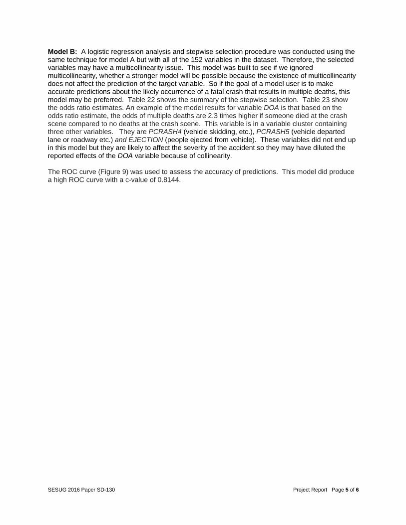
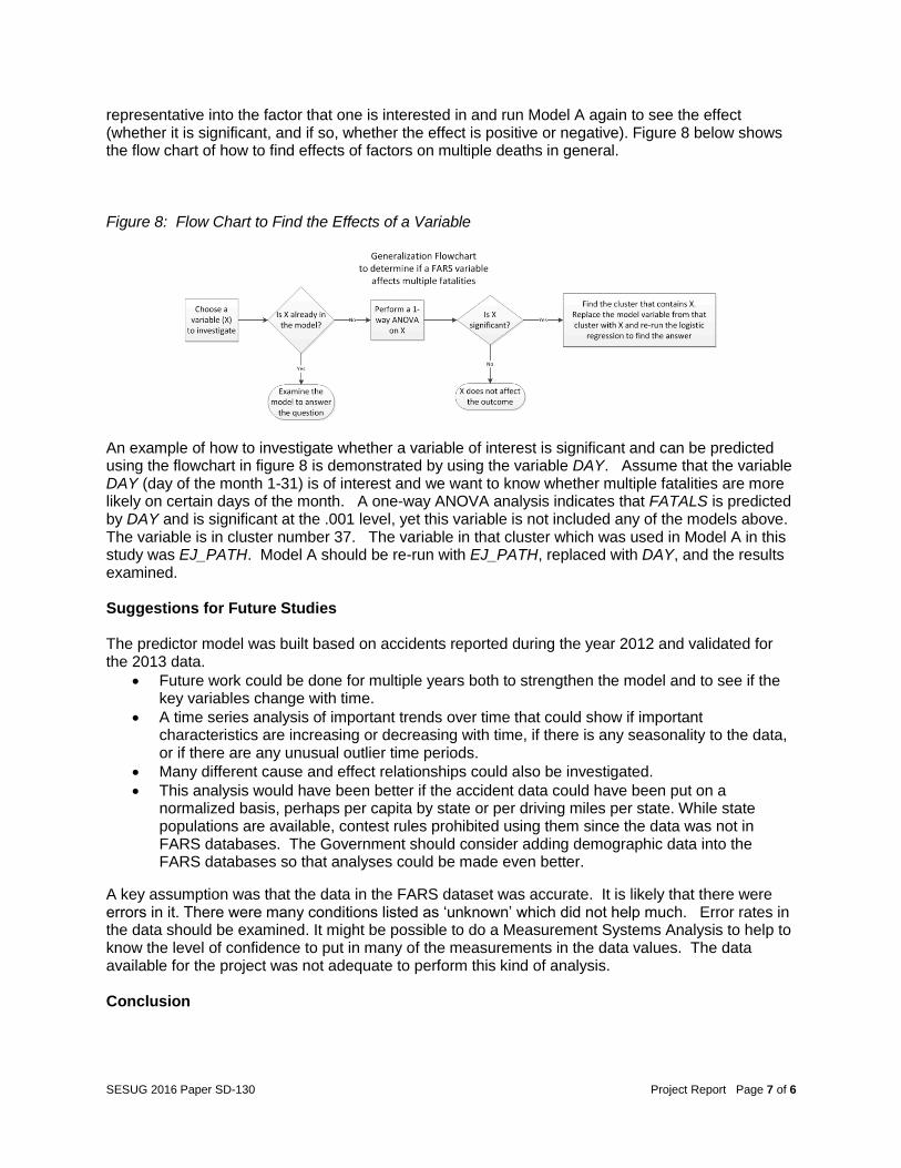
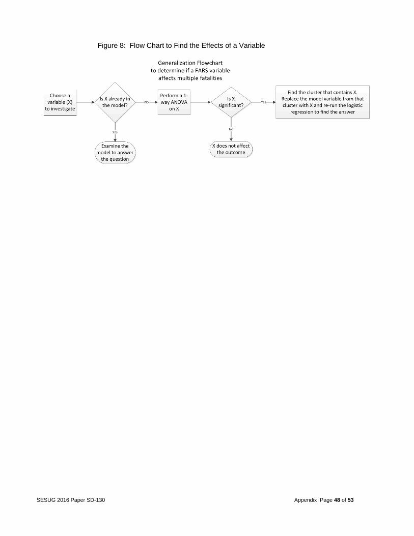
representative into the factor that one is interested in and run Model A again to see the effect (whether it is significant, and if so, whether the effect is positive or negative). Figure 8 below shows the flow chart of how to find effects of factors on multiple deaths in general. Figure 8: Flow Chart to Find the Effects of a Variable
An example of how to investigate whether a variable of interest is significant and can be predicted using the flowchart in figure 8 is demonstrated by using the variable DAY. Assume that the variable DAY (day of the month 1-31) is of interest and we want to know whether multiple fatalities are more likely on certain days of the month. A one-way ANOVA analysis indicates that FATALS is predicted by DAY and is significant at the .001 level, yet this variable is not included any of the models above. The variable is in cluster number 37. The variable in that cluster which was used in Model A in this study was EJ_PATH. Model A should be re-run with EJ_PATH, replaced with DAY, and the results examined. Suggestions for Future Studies The predictor model was built based on accidents reported during the year 2012 and validated for the 2013 data.
Future work could be done for multiple years both to strengthen the model and to see if the key variables change with time.
A time series analysis of important trends over time that could show if important characteristics are increasing or decreasing with time, if there is any seasonality to the data, or if there are any unusual outlier time periods.
Many different cause and effect relationships could also be investigated.
This analysis would have been better if the accident data could have been put on a normalized basis, perhaps per capita by state or per driving miles per state. While state populations are available, contest rules prohibited using them since the data was not in FARS databases. The Government should consider adding demographic data into the FARS databases so that analyses could be made even better.
A key assumption was that the data in the FARS dataset was accurate. It is likely that there were errors in it. There were many conditions listed as ‘unknown’ which did not help much. Error rates in the data should be examined. It might be possible to do a Measurement Systems Analysis to help to know the level of confidence to put in many of the measurements in the data values. The data available for the project was not adequate to perform this kind of analysis. Conclusion
SESUG 2016 Paper SD-130 Project Report Page 8 of 6
Since accidents are undesirable and unplanned, they can be prevented given the circumstances leading to the accident are recognized, and acted upon, prior to its occurrence. Model A and model B suggested that a number of factors contribute to the risk of multiple fatalities, including PERMVIT, INJ_SEV, PERNOTMVIT, DOA, PERSONS, NUMOCCS, FIRE_EXP, COUNTY, CITY, VE_TOTAL, DEFORMED, VSPD_LIM, HOUR, DRUNK_DR, etc. Model A would be ideal for a better understanding of effects of factors on multiple deaths while model B would be ideal for prediction purposes. Since the ROC curves for the 2012 and 2013 data were very similar, investigators can use previous year’s data to predict the following year’s data. This project also provided a general procedure for the users if any factor becomes of interest to them. This study is a step towards sensible analysis of the worst kind of motor vehicle fatalities and that all stakeholders in the transportation industry can be better informed and take sensible actions to help reduce them.
Appendix TABLE OF CONTENTS PAGE Tables Table 1: IMPACT1 in year 1999 2 Table 2: IMPACT1 in year 2012 3 Table 3: Before MVIOLATN is collapsed from VIOLATN database 4 Table 4: After MVIOLATN is collapsed into VIOLATN from the VIOLATN database 6 Table 5: Before MDRDSTRD categories are condensed from DISTRACT database 7 Table 6: After MDRDSTRD condensed in variable DISTRACT 8 Table 7: Before MFACTOR it was condensed from FACTOR database 9 Table 8: After MFACTOR was condensed into variable FACTOR from FACTOR database 10 Table 9: Before MDRMANAV is condensed from MANEUVER database 11 Table 10: After MDRMANAV is condensed into MANAV from MANEUVER database 12 Table 11: Before MVISOBSC is condensed from VISION database 13 Table 12: After MVISOBSC from VISION database is condensed into VIS 14 Table 13: List of variables dropped 15 Table 14: Table on variable FATALS 17 Table 15: Table on MULTIPLE 18 Table 16: List of categorical and Numeric Variables used in one-way ANOVA 19 Table 17: Tukey’s Table of WEATHER variable with all the 12 categories 23 Table 18: WEATHER Variable after Grouping 24 Table 19: Cluster grouping of the 152 Variables used in VARCLUS procedure 25 Table 20: Summary of Stepwise Selection for Model A 30 Table 21: Odds Ratio Estimate for Model A 31 Table 22: Summary of Stepwise Selection for Model B 34 Table 23: Odds Ratio Estimates for Model B 35 Table 24: MULTIPLE frequency after sampling 39
Figures Figure 1: FARS Data Base 40 Figure 2: Frequency of Accidents in the USA for years 2012 & 2013 41 Figure 3: Map of Georgia for years 2012 & 2013 42 Figure 4: Map of North Carolina for years 2012 & 2013 43 Figure 5: Map of California for years 2012 & 2013 44 Figure 6: Map of Wyoming for years 2012 & 2013 45 Figure 7: Histogram of variable VSPD_LIM 46 Figure 8: Flow Chart to Find the Effects of a Variable 47 Figure 9: ROC curves side by side comparison 48
SESUG 2016 Paper SD-130 Appendix Page 2 of 53
Figure 10: ROC Curve for 2013 Validation Data 49 SAS Code Summary of Coding Step 1: Filter First Event from datasets. 50 Step 2: ANOVA to check significant variables 50 Step 3: Clustering 51
SESUG 2016 Paper SD-130 Appendix Page 3 of 53
Table 1: IMPACT1 in year 1999
IMPACT1 Frequency Percent
0 3471 6.11
1 2980 5.24
2 1411 2.48
3 3221 5.67
4 502 0.88
5 539 0.95
6 2516 4.43
7 732 1.29
8 573 1.01
9 3976 7
10 1533 2.7
11 4238 7.46
12 28585 50.31
13 280 0.49
14 952 1.68
99 1311 2.31
SESUG 2016 Paper SD-130 Appendix Page 4 of 53
Table 2: IMPACT1 in year 2012
IMPACT1 Frequency Percent
0 3426 7.45
1 1649 3.59
2 610 1.33
3 1919 4.18
4 266 0.58
5 336 0.73
6 2614 5.69
7 452 0.98
8 352 0.77
9 2321 5.05
10 689 1.5
11 2018 4.39
12 24388 53.06
13 124 0.27
14 1093 2.38
18 87 0.19
61 672 1.46
62 369 0.8
63 187 0.41
81 564 1.23
82 340 0.74
83 141 0.31
98 658 1.43
99 685 1.49
SESUG 2016 Paper SD-130 Appendix Page 5 of 53
TABLE 3: Before MVIOLATN is collapsed from VIOLATN database
MVIOLATN Frequency Percent
0 40413 82.71
1 1260 2.58
2 326 0.67
3 233 0.48
4 429 0.88
5 30 0.06
6 2 0
7 354 0.72
8 65 0.13
9 152 0.31
11 1140 2.33
12 123 0.25
13 13 0.03
14 7 0.01
15 41 0.08
16 9 0.02
18 12 0.02
19 51 0.1
21 4 0.01
22 139 0.28
23 163 0.33
24 4 0.01
25 1 0
26 2 0
29 84 0.17
31 63 0.13
32 4 0.01
33 4 0.01
34 2 0
35 24 0.05
36 1 0
37 120 0.25
38 18 0.04
39 45 0.09
41 10 0.02
42 20 0.04
43 7 0.01
45 5 0.01
46 542 1.11
48 10 0.02
SESUG 2016 Paper SD-130 Appendix Page 6 of 53
49 68 0.14
51 21 0.04
52 110 0.23
53 36 0.07
54 1 0
55 2 0
56 1 0
58 48 0.1
59 20 0.04
61 36 0.07
62 16 0.03
66 1 0
69 218 0.45
71 192 0.39
72 349 0.71
73 18 0.04
74 89 0.18
75 68 0.14
76 201 0.41
79 80 0.16
81 13 0.03
82 19 0.04
83 213 0.44
84 8 0.02
86 5 0.01
89 64 0.13
91 5 0.01
92 13 0.03
93 9 0.02
95 252 0.52
97 19 0.04
98 50 0.1
99 687 1.41
SESUG 2016 Paper SD-130 Appendix Page 7 of 53
Table 4: After MVIOLATN is collapsed into VIOLATN from the VIOLATN database
VIOLATN
MV Frequency Percent
EQUIPMENT 303 0.63
IMPAIRMENT 1328 2.76
LANE 271 0.56
LICENSE 836 1.74
NONE 40413 84.14
OTHER 1027 2.14
RECKLESS 2288 4.76
SPEED 393 0.82
TRAFFIC 281 0.59
TURNING 656 1.37
WRONG 236 0.49
SESUG 2016 Paper SD-130 Appendix Page 8 of 53
Table 5: Before MDRDSTRD categories are condensed from DISTRACT database
MDRDSTRD Frequency Percent
0 33152 72.08
1 366 0.8
3 148 0.32
4 15 0.03
5 113 0.25
6 106 0.23
7 54 0.12
9 28 0.06
10 68 0.15
12 205 0.45
13 39 0.08
14 16 0.03
15 180 0.39
16 252 0.55
17 255 0.55
18 15 0.03
19 76 0.17
92 446 0.97
93 1186 2.58
96 4063 8.83
97 11 0.02
98 242 0.53
99 4959 10.78
SESUG 2016 Paper SD-130 Appendix Page 9 of 53
Table 6: After MDRDSTRD condensed in variable DISTRACT
DISTRACT Frequency Percent
0 76331 99.86
30 105 0.14
SESUG 2016 Paper SD-130 Appendix Page 10 of 53
Table 7: Before MFACTOR it was condensed from FACTOR database
MFACTOR Frequency Percent
0 43025 93.45
1 672 1.46
2 135 0.29
3 30 0.07
4 12 0.03
5 23 0.05
6 2 0
7 52 0.11
8 14 0.03
9 32 0.07
11 17 0.04
SESUG 2016 Paper SD-130 Appendix Page 11 of 53
Table 8: After MFACTOR was condensed into variable FACTOR from FACTOR database
FACTOR Frequency Percent
0 65181 93.14
1 4705 6.72
2 85 0.12
3 8 0.01
4 2 0
5 1 0
SESUG 2016 Paper SD-130 Appendix Page 12 of 53
Table 9: Before MDRMANAV is condensed from MANEUVER database
MDRMANAV Frequency Percent
0 39023 84.88
1 78 0.17
2 24 0.05
3 124 0.27
4 2565 5.58
5 504 1.1
92 277 0.6
95 252 0.55
98 1954 4.25
99 1176 2.56
SESUG 2016 Paper SD-130 Appendix Page 13 of 53
Table 10: After MDRMANAV is condensed into MANAV from MANEUVER database
MANAV Frequency Percent
0 59753 85.38
2 46 0.07
3 236 0.34
30 5267 7.53
95 108 0.15
98 2914 4.16
99 1658 2.37
SESUG 2016 Paper SD-130 Appendix Page 14 of 53
Table 11: Before MVISOBSC is condensed from VISION database
MVISOBSC Frequency Percent
0 43110 93.72
1 400 0.87
2 208 0.45
3 154 0.33
4 17 0.04
5 68 0.15
6 216 0.47
7 52 0.11
8 3 0.01
9 2 0
10 4 0.01
11 5 0.01
13 12 0.03
14 13 0.03
95 252 0.55
SESUG 2016 Paper SD-130 Appendix Page 15 of 53
Table 12: After MVISOBSC from VISION database is condensed into VIS
VIS Frequency Percent
0 66264 94.69
1 589 0.84
2 275 0.39
3 226 0.32
4 23 0.03
5 80 0.11
6 327 0.47
SESUG 2016 Paper SD-130 Appendix Page 16 of 53
Table 13: List of variables dropped
VE_FORMS
PEDS
NHS
TWAY_ID
TWAY_ID2
MILEPT
RAIL
MAK_MOD
VIN
VIN_1
VIN_2
VIN_3
VIN_4
VIN_5
VIN_6
VIN_7
VIN_8
VIN_9
VIN_10
VIN_11
VIN_12
VINTYPE
VINMAKE
VINA_MOD
VIN_BT
VINMODYR
VIN_LNGT
VIN_WGT
VINTYPE
VINMAKE
VINA_MOD
VIN_BT
VINMODYR
VIN_LNGT
VIN_WGT
WHLBS_LG
WHLBS_SH
SER_TR
MCYCL_DS
CARBUR
CYLINDER
MCYCL_CY
MCYCL_WT
TIRE_SZE
TON_RAT
TRK_WT
TRKWTVAR
VIN_REST
WHLDRWHL
MCARR_I1
MCARR_I2
SESUG 2016 Paper SD-130 Appendix Page 17 of 53
MCARR_ID
HAZ_ID
HAZ_CNO
FIRST_MO
FIRST_YR
LAST_MO
LAST_YR
_NAME_
DRUG_DET
DSTATUS
DRUGTST1
DRUGTST2
DRUGTST3
DRUGRES1
DRUGRES2
DRUGRES3
HOSPITAL
DEATH_DA
DEATH_MO
DEATH_HR
DEATH_MN
DEATH_TM
P_SF1
P_SF2
P_SF3
CERT_NO
HISPANIC
RACE
PVIN
PVIN_1
PVIN_2
PVIN_3
PVIN_4
PVIN_5
PVIN_6
PVIN_7
PVIN_8
PVIN_9
PVIN_10
PVIN_11
PVIN_12
SESUG 2016 Paper SD-130 Appendix Page 18 of 53
Table 14: Table on variable FATALS
FATALS Frequency Percent
1 67289 88.03
2 7065 9.24
3 1220 1.6
4 531 0.69
5 153 0.2
6 26 0.03
7 65 0.09
9 64 0.08
15 23 0.03
SESUG 2016 Paper SD-130 Appendix Page 19 of 53
Table 15: Table on MULTIPLE
MULTIPLE Frequency Percent Cumulative Frequency
Cumulative Percent
0 67289 88.03 67289 88.03
1 9147 11.97 76436 100
SESUG 2016 Paper SD-130 Appendix Page 20 of 53
Table 16: List of categorical and Numeric Variables used in one-way ANOVA
No Variable Type
1 CRSH_0 Categorical
2 DR_DRINK Categorical
3 DR_PRES Categorical
4 DR_ZIP Categorical
5 FIRE_EXP Categorical
6 HAZ_INV Categorical
7 HIT_RUN Categorical
8 IMPAIR_0 Categorical
9 J_KNIFE Categorical
10 MANAV Categorical
11 P_CRASH1 Categorical
12 REST_MIS Categorical
13 ROLLOVER Categorical
14 SAFE_1 Categorical
15 SPEEDREL Categorical
16 UNITTYPE Categorical
17 VALIGN Categorical
18 VNUM_LAN Categorical
19 VPROFILE Categorical
20 VTRAFWAY Categorical
21 DAMAGEN Categorical
22 DAM_1 Categorical
23 DAM_2 Categorical
24 DAM_3 Categorical
25 DAM_4 Categorical
26 DAM_5 Categorical
27 DAM_6 Categorical
28 DAM_13 Categorical
29 DAM_14 Categorical
30 DR_SF4 Categorical
34 PERMVIT Categorical
35 PERSONS Categorical
36 CEVENT_SOE Categorical
37 P_CRASH2 Categorical
38 RELJCT2 Categorical
39 VEVENT_SOE Categorical
40 L_STATE Categorical
SESUG 2016 Paper SD-130 Appendix Page 21 of 53
41 NUMOCCS Categorical
42 REG_STAT Categorical
43 DISPLACEN Categorical
44 GVWR Categorical
45 V_CONFIG Categorical
46 DEFORMED Categorical
47 HARM_EV Categorical
48 PERNOTMVIT Categorical
49 REST_USE Categorical
50 TOWED Categorical
51 VIS Categorical
52 WEATHER Categorical
53 WEATHER1 Categorical
54 CRSH_1 Categorical
55 CRSH_2 Categorical
56 CRSH_12 Categorical
57 CRSH_19 Categorical
58 IMPAIR_9 Categorical
59 PRIOR_3 Categorical
60 EXTRICAT Categorical
61 INJ_SEV Categorical
62 WORK_INJ Categorical
63 MODEL Categorical
64 REL_ROAD Categorical
65 ROAD_FNC Categorical
66 ROUTE Categorical
67 VIOLATN_LANE Categorical
69 DRINKING Categorical
70 DRUGS Categorical
71 CRSH_99 Categorical
72 PRIOR_99 Categorical
73 SAFE_9 Categorical
74 CRSH_5 Categorical
75 PRIOR_11 Categorical
76 CF1 Categorical
77 CF2 Categorical
78 CRSH_4 Categorical
79 IMPAIR_8 Categorical
80 PRIOR_8 Categorical
SESUG 2016 Paper SD-130 Appendix Page 22 of 53
81 DOA Categorical
82 EJECTION Categorical
83 PCRASH4 Categorical
84 PCRASH5 Categorical
85 CRSH_98 Categorical
86 PRIOR_98 Categorical
87 CRSH_9 Categorical
88 PRIOR_6 Categorical
89 PRIOR_5 Categorical
90 SAFE_2 Categorical
91 DAM_7 Categorical
92 DAM_8 Categorical
93 DAM_9 Categorical
94 DAM_10 Categorical
95 DAM_11 Categorical
96 DAM_30 Categorical
100 DRUNK_DR Categorical
101 VE_TOTAL Categorical
102 DAM_12 Categorical
103 IMPACT1 Categorical
104 TRAV_SP Categorical
106 L_TYPE Categorical
107 VIOLATN_RECKLESS Categorical
108 CRSH_21 Categorical
109 PRIOR_14 Categorical
112 STATE Categorical
113 IMPAIR_98 Categorical
114 SAFE_8 Categorical
115 CARGO_BT Categorical
116 SEAT_POS Categorical
117 CITY Categorical
118 COUNTY Categorical
119 PRIOR_2 Categorical
120 DRIMP_NONE Categorical
121 L_COMPL Categorical
122 VIOLATN_NONE Categorical
123 OWNER Categorical
124 IMPAIR_99 Categorical
127 DAY Categorical
SESUG 2016 Paper SD-130 Appendix Page 23 of 53
128 DR_SF1 Categorical
129 EJ_PATH Categorical
130 SAFE_3 Categorical
131 WRK_ZONE Categorical
132 BODY_TYP Categorical
133 BUS_USE Categorical
134 MONTH Categorical
135 VSURCOND Categorical
136 DAY_WEEK Categorical
137 HOLIDA Categorical
138 PRIOR_4 Categorical
139 IMPAIR_96 Categorical
140 ALC_STATUS Categorical
141 SEX Categorical
142 CRSH_6 Categorical
143 CRSH_3 Categorical
144 DISTRACT Categorical
145 VIOLATN_TRAFFIC Categorical
146 FUELCODEN Categorical
147 VEH_SC1 Categorical
148 SP_JUR Categorical
149 TYP_INT Categorical
150 PREV_OTH Categorical
31 ARR_HOUR Numeric
32 HOUR Numeric
33 NOT_HOUR Numeric
68 VSPD_LIM Numeric
97 ARR_MIN Numeric
98 MINUTE Numeric
99 NOT_MIN Numeric
105 AGE Numeric
110 HOSP_HR Numeric
111 HOSP_MN Numeric
125 LAG_HRS Numeric
126 LAG_MINS Numeric
151 DR_HGT Numeric
152 DR_WGT Numeric
SESUG 2016 Paper SD-130 Appendix Page 24 of 53
Table 17: Tukey’s Table of WEATHER variable with all the 12 categories
Tukey Grouping Mean N Weather
A 1.45161 31 7
A
B A 1.36957 92 11
B A
B A 1.3669 1022 5
B
B C 1.193 11975 10
B C
B C 1.18321 131 6
B C
B C 1.18067 952 4
B C
B C 1.17251 5165 2
B C
B C 1.16276 56360 1
B C
B C 1.15116 172 3
C
C 1.11151 278 99
C
C 1.06742 178 98
C
C 1 80 8
SESUG 2016 Paper SD-130 Appendix Page 25 of 53
Table 18: WEATHER Variable after Grouping
Significant Var WEATHER
TUKEY GROUPING
7,11,5 A
10,6,4,2,1,3 B
99,98,8 C
SESUG 2016 Paper SD-130 Appendix Page 26 of 53
Table 19: Cluster grouping of the 152 Variables used in VARCLUS procedure
Cluster Variable Own Next 1-R**2 Label
Cluster
Cluster
Cluster 2 PREV_OTH 0.0003 0.0002 0.9999 Previous other harmful MV convictions
NOT_MIN 0.6253 0.159 0.4455 Notification Time EMS (MIN)
TYP_INT 0.5256 0.0077 0.4781 Type of Intersection
DR_DRINK 0.9816 0.4938 0.0363 Driver Drinking
DAM_4 0.8289 0.4177 0.2939
Cluster 3 NOT_HOUR 0.8084 0.2968 0.2725 Notification Time EMS (HOUR)
Cluster 4 PERMVIT 0.9803 0.4038 0.0331 Number of Persons in Motor Vehicles In-Transport
VEVENT_SOE
0.9015 0.028 0.1014 Sequence of Events
Cluster 6 BODY_TYP 0.7225 0.1127 0.3127 Body Type
DISPLACEN 0.7386 0.0388 0.272
DEFORMED 0.7984 0.2394 0.265 Extent of Damage
WEATHER 0.908 0.0349 0.0953 Atmospheric Conditions
PRIOR_3 0.7323 0.4723 0.5073
Cluster 11 INJ_SEV 0.8497 0.1705 0.1812 Injury Severity
VSPD_LIM 0.5912 0.0158 0.4154 Speed Limit
ROUTE 0.6503 0.0171 0.3558 Route Signing
Cluster 13 DRINKING 0.849 0.0337 0.1563 Police Reported Alcohol Involvement
DRUGS 0.849 0.0137 0.1531 Police Reported Drug Involvement
PRIOR_99 0.6846 0.0194 0.3216
Cluster 15 CRSH_5 0.7544 0.0052 0.2469
Cluster 16 CF1 0.7758 0.0038 0.225 Related Factors (1)
Cluster 17 CRSH_4 0.7583 0.1062 0.2704
PCRASH5 0.5685 0.1753 0.5232 Pre- Impact Location
PRIOR_98 0.6818 0.0096 0.3213
Cluster 20 CRSH_9 0.6681 0.0192 0.3384
SAFE_2 0.6283 0.0209 0.3796
DAM_8 0.8588 0.5192 0.2937
Cluster 23 SP_JUR 0.5256 0.0016 0.4752 Special Jurisdiction
Cluster 24 MINUTE 1 0.0167 0 Crash Time (MINUTE)
DRUNK_DR 0.797 0.0621 0.2164 Drunk Drivers
SESUG 2016 Paper SD-130 Appendix Page 27 of 53
Cluster 26 HOUR 1 0.0754 0 Crash Time (HOUR)
DAM_12 0.764 0.1431 0.2754
Cluster 28 AGE 0.4957 0.0506 0.5311 Age
Cluster 29 CRSH_21 0.6198 0.0327 0.393
Cluster 30 IMPAIR_98 0.6379 0.1242 0.4135
Cluster 31 SEAT_POS 0.6698 0.0912 0.3633 Seating Position
L_STATE 0.7756 0.1976 0.2797 Driver License State
Cluster 33 PRIOR_2 1 0.0097 0
Cluster 34 OWNER 1 0.0637 0 Registered Vehicle Owner
DRIMP_NONE
0.5255 0.133 0.5473
Cluster 36 IMPAIR_99 1 0.1777 0
Cluster 37 LAG_HRS 0.6061 0.0328 0.4072 Crash to Death Time (Hours)
Cluster 38 CITY 1 0.0309 0 City
EJ_PATH 0.5135 0.0203 0.4965 Ejection Path
Cluster 40 WRK_ZONE 0.5488 0.0044 0.4532 Work Zone
VSURCOND 0.532 0.0365 0.4857 Roadway surface Condition
HOSP_HR 0.7856 0.3905 0.3518 EMS time at Hospital (HOUR)
HOSP_MN 0.7804 0.2005 0.2746 EMS time at Hospital (MIN)
Cluster 43 DAY_WEEK 0.5394 0.0138 0.467 Crash Date (Day of Week)
Cluster 45 PRIOR_4 1 0.0066 0
Cluster 46 IMPAIR_96 1 0.005 0
ALC_STATUS
0.5169 0.0103 0.4881 Alcohol Test- Status
Cluster 48 CRSH_6 1 0.019 0
Cluster 49 CRSH_3 1 0.0405 0
Cluster 50 DISTRACT 0.5015 0.0002 0.4986
Cluster 51 FUELCODEN
1 0.0001 0
Cluster 52 VEH_SC1 1 0.0091 0 Vehicle Related factors (1)
Cluster 53 DR_SF4 1 0.0005 0 Driver Related Factors (4 choices)
Cluster 1 ROLLOVER 0.5347 0.2812 0.6473 Rollover Type
FIRE_EXP 0.3191 0.1537 0.8046 Fire Occurrence
REST_MIS 0.9594 0.5143 0.0837
SESUG 2016 Paper SD-130 Appendix Page 28 of 53
UNITTYPE 0.9816 0.4938 0.0363 Unit Type
HIT_RUN 0.7666 0.4502 0.4245 Hit and Run
J_KNIFE 0.9685 0.4863 0.0614 Jackknife
HAZ_INV 0.9816 0.4938 0.0363
DR_PRES 0.966 0.4849 0.066 Driver Presence
DR_ZIP 0.2487 0.1098 0.844 Driver ZIP Code
SPEEDREL 0.7501 0.3866 0.4074 Speed Related
VTRAFWAY 0.9751 0.4853 0.0484 Trafficway Description
VNUM_LAN 0.7241 0.3437 0.4204 Total Lanes in Roadway
VALIGN 0.972 0.4828 0.0541 Roadway Alignment
VPROFILE 0.7561 0.3607 0.3816 Roadway Grade
P_CRASH1 0.8342 0.4022 0.2773 Pre-Event movement
MANAV 0.4698 0.2137 0.6743
CRSH_0 0.2723 0.1063 0.8143
IMPAIR_0 0.474 0.1912 0.6503
SAFE_1 0.7051 0.4069 0.4973
DAM_1 0.627 0.309 0.5398
DAM_2 0.7597 0.3796 0.3874
DAM_3 0.6884 0.3022 0.4465
DAM_5 0.8026 0.4081 0.3335
DAM_6 0.5522 0.3637 0.7038
DAM_13 0.5427 0.3767 0.7336
DAM_14 0.6391 0.4398 0.6442
damagen 0.6922 0.4867 0.5997
ARR_HOUR 0.81 0.3168 0.2781 Arrival Time EMS (HOUR)
ARR_MIN 0.6191 0.1598 0.4533 Arrival Time EMS (MIN)
PERSONS 0.9803 0.4135 0.0336 Number of MV occupant
Cluster 5 P_CRASH2 0.3403 0.0275 0.6783 Critical Event - Precrash (Event)
RELJCT2 0.1679 0.0084 0.8391 Relation to Junction - Specific Location
CEVENT_SOE
0.8921 0.0318 0.1115 Sequence of Events
BUS_USE 0.7225 0.1788 0.3379 Bus Use
Cluster 7 GVWR 0.7521 0.143 0.2892 Gross vehicle weight rating
V_CONFIG 0.291 0.0066 0.7137 Vehicle Configuration
Cluster 8 HARM_EV 0.5846 0.1961 0.5167 First Harmful Event
SESUG 2016 Paper SD-130 Appendix Page 29 of 53
REST_USE 0.1197 0.1328 1.0152 Restraint System/Helmet Use
TOWED 0.7931 0.2252 0.267 Vehicle Removal
PERNOTMVIT
0.6074 0.2431 0.5187
Cluster 9 WEATHER1 0.9054 0.0323 0.0977 Atmospheric Conditions
VIS 0.3211 0.0666 0.7274
Cluster 10 CRSH_12 0.407 0.1186 0.6728
CRSH_2 0.4526 0.2115 0.6942
CRSH_1 0.2766 0.1072 0.8103
CRSH_19 0.2368 0.1277 0.875
IMPAIR_9 0.2717 0.1086 0.817
EXTRICAT 0.1932 0.0504 0.8496 Extrication
WORK_INJ 0.814 0.1577 0.2208 Fatal Injury at work
Cluster 12 ROAD_FNC 0.6139 0.0179 0.3931 Roadway Function Class
MODEL 0.0002 0.0001 1 Vehicle Model
REL_ROAD 0.1411 0.0261 0.8818 Relation To Trafficway
VIOLATN_LANE
0.0029 0.0069 1.004
Cluster 14 CRSH_99 0.6765 0.035 0.3353
SAFE_9 0.1765 0.0099 0.8317
PRIOR_11 0.7544 0.0068 0.2473
CF2 0.7758 0.0105 0.2265 Related Factors (2)
IMPAIR_8 0.0771 0.0072 0.9296
PRIOR_8 0.7542 0.1081 0.2756
Cluster 18 EJECTION 0.4014 0.0501 0.6302 Ejection
DOA 0.2834 0.3538 1.1089 Died at scene/en route
PCRASH4 0.4188 0.0481 0.6106 Pre- Impact Stability
Cluster 19 CRSH_98 0.6818 0.0183 0.3241
PRIOR_6 0.6681 0.0273 0.3412
Cluster 21 PRIOR_5 0.6283 0.1218 0.4232
Cluster 22 DAM_11 0.6736 0.3499 0.502
DAM_7 0.8084 0.5245 0.403
DAM_9 0.7614 0.3798 0.3847
DAM_10 0.8272 0.449 0.3136
DAM_30 0.0216 0.0311 1.0098
Cluster 25 VE_TOTAL 0.797 0.0766 0.2198 Number of vehicle forms submitted
Cluster 27 IMPACT1 0.766 0.2017 0.2931 Area of Impact- Initial Contact Point
TRAV_SP 0.0064 0.0055 0.9991 Travel Speed
SESUG 2016 Paper SD-130 Appendix Page 30 of 53
L_TYPE 0.4446 0.0415 0.5795 Non-CDL license Type
VIOLATN_RECKLESS
0.2235 0.0479 0.8155
PRIOR_14 0.6198 0.039 0.3956
SAFE_8 0.6379 0.1754 0.4392
CARGO_BT 0.6698 0.1153 0.3732 Cargo Body Type
Cluster 32 NUMOCCS 0.5007 0.7887 2.363 Number of Occupants
REG_STAT 0.6362 0.1148 0.411 Vehicle Registration State
Cluster 35 L_COMPL 0.6131 0.3075 0.5587 License Compliance with class of vehicle
VIOLATN_NONE
0.5862 0.3458 0.6324
LAG_MINS 0.6061 0.0452 0.4125 Crash to Death Minutes (Minutes)
Cluster 39 DAY 0.0607 0.0093 0.9481 Crash Date (DAY)
DR_SF1 0.5205 0.1024 0.5342 Driver Related Factors (4 choices)
SAFE_3 0.5488 0.0127 0.457
Cluster 41 MONTH 0.532 0.0377 0.4863 Crash Date (MONTH)
Cluster 42 STATE 0.2172 0.0221 0.8005 State Number
HOLIDA 0.5394 0.0445 0.4821
Cluster 44 COUNTY 1 0.0549 0 County
Cluster 47 SEX 0.5169 0.0167 0.4913 Sex
VIOLATN_TRAFFIC
0.5015 0.0025 0.4998
SESUG 2016 Paper SD-130 Appendix Page 31 of 53
Table 20: Summary of Stepwise Selection for Model A
Summary of Stepwise Selection
Step
Effect
DF Number
In
Score Chi-
Square
Wald Chi-
Square Pr >
ChiSq Variable
Label
Entered Removed
1 PERMVIT 9 1 2990.1317 <.0001 Number of Persons in Motor Vehicles In-Transport
2 INJ_SEV 1 2 1287.1013 <.0001 Injury Severity
3 CITY 1 3 209.0768 <.0001 City
4 DEFORMED 2 4 166.9710 <.0001 Extent of Damage
5 VSPD_LIM 16 5 216.1523 <.0001 Speed Limit
6 HOUR 1 6 111.1223 <.0001 Crash Time (HOUR)
7 DRIMP_NONE 1 7 61.6409 <.0001
8 DRINKING 2 8 65.1708 <.0001 Police Reported Alcohol Use
9 PRIOR_3 1 9 58.3525 <.0001
10 DISPLACEN 1 10 41.8751 <.0001
11 DRUNK_DR 2 11 40.4049 <.0001 Drunk Drivers
12 DAY_WEEK 2 12 32.7051 <.0001 Crash Date (Day of Week)
13 DAM_8 1 13 27.3820 <.0001
14 CF1 19 14 65.3254 <.0001 Related Factors (1)
15 ROUTE 2 15 27.6672 <.0001 Route Signing
16 DR_DRINK 1 16 17.6369 <.0001 Driver Drinking
17 PCRASH5 1 17 15.1368 <.0001 Pre- Impact Location
18 HOSP_MN 1 18 12.5065 0.0004 EMS time at Hospital (MIN)
19 LAG_HRS 1 19 11.3204 0.0008 Crash to Death Time (Hours)
20 DAM_12 1 20 10.2514 0.0014
21 IMPAIR_99 1 21 10.0619 0.0015
22 OWNER 1 22 7.7191 0.0055 Registered Vehicle Owner
23 PRIOR_98 1 23 7.0661 0.0079
24 PRIOR_98 1 22 0.0036 0.9524
SESUG 2016 Paper SD-130 Appendix Page 32 of 53
Table 21: Odds Ratio Estimate for Model A
Odds Ratio Estimates
Effect Point Estimate 95% Wald
Confidence Limits
DR_DRINK 1 vs 99 0.453 0.350 0.588
PERMVIT 9 vs 50 11.191 9.956 12.579
PERMVIT 17 vs 50 >999.999 <0.001 >999.999
PERMVIT 18 vs 50 36.463 10.931 121.638
PERMVIT 21 vs 50 6.072 5.551 6.642
PERMVIT 23 vs 50 >999.999 <0.001 >999.999
PERMVIT 24 vs 50 76.929 41.921 141.170
PERMVIT 26 vs 50 >999.999 <0.001 >999.999
PERMVIT 33 vs 50 3.653 <0.001 >999.999
PERMVIT 47 vs 50 >999.999 <0.001 >999.999
DEFORMED 2 vs 6 0.567 0.486 0.661
DEFORMED 4 vs 6 0.636 0.563 0.719
PRIOR_3 0 vs 1 3.496 2.524 4.844
INJ_SEV 2 vs 6 0.320 0.294 0.348
ROUTE 1 vs 3 0.869 0.766 0.986
ROUTE 2 vs 3 1.205 1.103 1.315
VSPD_LIM 0 vs 80 0.194 0.076 0.500
VSPD_LIM 5 vs 80 <0.001 <0.001 >999.999
VSPD_LIM 10 vs 80 0.186 0.034 1.013
VSPD_LIM 15 vs 80 0.179 0.049 0.648
VSPD_LIM 20 vs 80 0.232 0.069 0.778
VSPD_LIM 25 vs 80 0.223 0.096 0.518
VSPD_LIM 30 vs 80 0.252 0.109 0.582
VSPD_LIM 35 vs 80 0.189 0.083 0.433
VSPD_LIM 40 vs 80 0.250 0.109 0.575
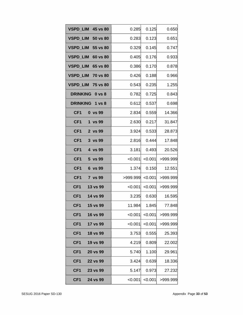
SESUG 2016 Paper SD-130 Appendix Page 33 of 53
VSPD_LIM 45 vs 80 0.285 0.125 0.650
VSPD_LIM 50 vs 80 0.283 0.123 0.651
VSPD_LIM 55 vs 80 0.329 0.145 0.747
VSPD_LIM 60 vs 80 0.405 0.176 0.933
VSPD_LIM 65 vs 80 0.386 0.170 0.878
VSPD_LIM 70 vs 80 0.426 0.188 0.966
VSPD_LIM 75 vs 80 0.543 0.235 1.255
DRINKING 0 vs 8 0.782 0.725 0.843
DRINKING 1 vs 8 0.612 0.537 0.698
CF1 0 vs 99 2.834 0.559 14.366
CF1 1 vs 99 2.630 0.217 31.847
CF1 2 vs 99 3.924 0.533 28.873
CF1 3 vs 99 2.816 0.444 17.848
CF1 4 vs 99 3.181 0.493 20.526
CF1 5 vs 99 <0.001 <0.001 >999.999
CF1 6 vs 99 1.374 0.150 12.551
CF1 7 vs 99 >999.999 <0.001 >999.999
CF1 13 vs 99 <0.001 <0.001 >999.999
CF1 14 vs 99 3.235 0.630 16.595
CF1 15 vs 99 11.984 1.845 77.848
CF1 16 vs 99 <0.001 <0.001 >999.999
CF1 17 vs 99 <0.001 <0.001 >999.999
CF1 18 vs 99 3.753 0.555 25.393
CF1 19 vs 99 4.219 0.809 22.002
CF1 20 vs 99 5.740 1.100 29.961
CF1 22 vs 99 3.424 0.639 18.336
CF1 23 vs 99 5.147 0.973 27.232
CF1 24 vs 99 <0.001 <0.001 >999.999
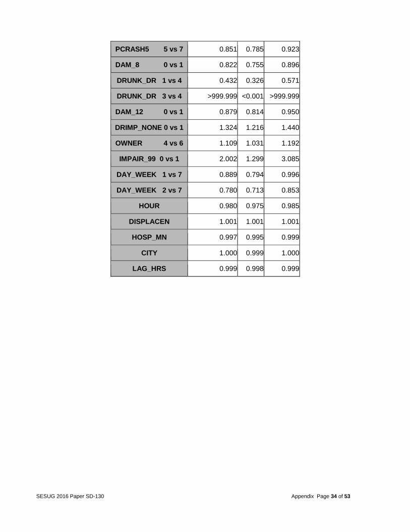
SESUG 2016 Paper SD-130 Appendix Page 34 of 53
PCRASH5 5 vs 7 0.851 0.785 0.923
DAM_8 0 vs 1 0.822 0.755 0.896
DRUNK_DR 1 vs 4 0.432 0.326 0.571
DRUNK_DR 3 vs 4 >999.999 <0.001 >999.999
DAM_12 0 vs 1 0.879 0.814 0.950
DRIMP_NONE 0 vs 1 1.324 1.216 1.440
OWNER 4 vs 6 1.109 1.031 1.192
IMPAIR_99 0 vs 1 2.002 1.299 3.085
DAY_WEEK 1 vs 7 0.889 0.794 0.996
DAY_WEEK 2 vs 7 0.780 0.713 0.853
HOUR 0.980 0.975 0.985
DISPLACEN 1.001 1.001 1.001
HOSP_MN 0.997 0.995 0.999
CITY 1.000 0.999 1.000
LAG_HRS 0.999 0.998 0.999
SESUG 2016 Paper SD-130 Appendix Page 35 of 53
Table 22: Summary of Stepwise Selection for Model B
Summary of Stepwise Selection
Step
Effect
DF Number
In
Score Chi-
Square
Wald Chi-
Square Pr >
ChiSq Variable
Label Entered Removed
1 PERMVIT 9 1 2990.1317 <.0001 Number of Persons in Motor Vehicles In-Transport
2 INJ_SEV 1 2 1287.1013 <.0001 Injury Severity
3 PERSONS 2 3 627.5972 <.0001 Number of MV occupant
4 PERNOTMVIT 2 4 453.5760 <.0001 Number of Persons Not in Motor Vehicles In-Transport
5 DOA 2 5 435.2631 <.0001 Died at scene/en route
6 FIRE_EXP 2 6 304.8571 <.0001 Fire Occurrence
7 CITY 2 7 162.1558 <.0001 City
8 COUNTY 3 8 163.2669 <.0001 County
9 HARM_EV 3 9 105.9981 <.0001 First Harmful Event
10 VSPD_LIM 16 10 142.9096 <.0001 Speed Limit
11 DRIMP_NONE 1 11 62.7570 <.0001
12 STATE 50 12 178.4668 <.0001 State Number
13 EXTRICAT 1 13 54.0121 <.0001 Extrication
14 TRAV_SP 2 14 51.8671 <.0001 Travel Speed
15 DAMAGE 2 15 49.6337 <.0001
16 VE_TOTAL 3 16 51.8259 <.0001 Number of vehicle forms submitted
17 VE_TOTAL 3 15 0.0257 0.9989 Number of vehicle forms submitted
SESUG 2016 Paper SD-130 Appendix Page 36 of 53
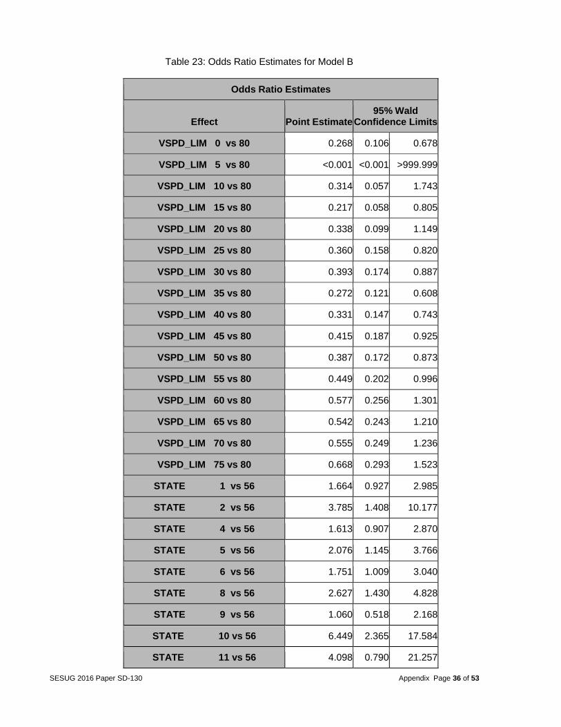
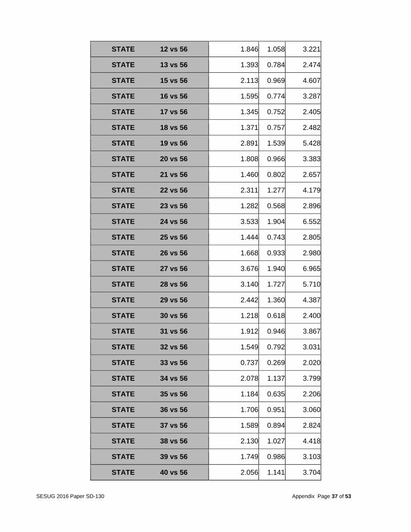
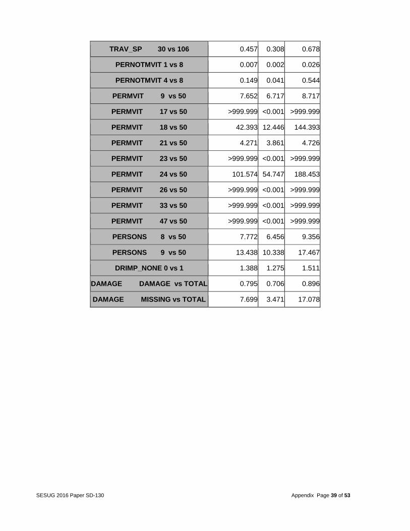
Table 23: Odds Ratio Estimates for Model B
Odds Ratio Estimates
Effect Point Estimate 95% Wald
Confidence Limits
VSPD_LIM 0 vs 80 0.268 0.106 0.678
VSPD_LIM 5 vs 80 <0.001 <0.001 >999.999
VSPD_LIM 10 vs 80 0.314 0.057 1.743
VSPD_LIM 15 vs 80 0.217 0.058 0.805
VSPD_LIM 20 vs 80 0.338 0.099 1.149
VSPD_LIM 25 vs 80 0.360 0.158 0.820
VSPD_LIM 30 vs 80 0.393 0.174 0.887
VSPD_LIM 35 vs 80 0.272 0.121 0.608
VSPD_LIM 40 vs 80 0.331 0.147 0.743
VSPD_LIM 45 vs 80 0.415 0.187 0.925
VSPD_LIM 50 vs 80 0.387 0.172 0.873
VSPD_LIM 55 vs 80 0.449 0.202 0.996
VSPD_LIM 60 vs 80 0.577 0.256 1.301
VSPD_LIM 65 vs 80 0.542 0.243 1.210
VSPD_LIM 70 vs 80 0.555 0.249 1.236
VSPD_LIM 75 vs 80 0.668 0.293 1.523
STATE 1 vs 56 1.664 0.927 2.985
STATE 2 vs 56 3.785 1.408 10.177
STATE 4 vs 56 1.613 0.907 2.870
STATE 5 vs 56 2.076 1.145 3.766
STATE 6 vs 56 1.751 1.009 3.040
STATE 8 vs 56 2.627 1.430 4.828
STATE 9 vs 56 1.060 0.518 2.168
STATE 10 vs 56 6.449 2.365 17.584
STATE 11 vs 56 4.098 0.790 21.257
SESUG 2016 Paper SD-130 Appendix Page 37 of 53
STATE 12 vs 56 1.846 1.058 3.221
STATE 13 vs 56 1.393 0.784 2.474
STATE 15 vs 56 2.113 0.969 4.607
STATE 16 vs 56 1.595 0.774 3.287
STATE 17 vs 56 1.345 0.752 2.405
STATE 18 vs 56 1.371 0.757 2.482
STATE 19 vs 56 2.891 1.539 5.428
STATE 20 vs 56 1.808 0.966 3.383
STATE 21 vs 56 1.460 0.802 2.657
STATE 22 vs 56 2.311 1.277 4.179
STATE 23 vs 56 1.282 0.568 2.896
STATE 24 vs 56 3.533 1.904 6.552
STATE 25 vs 56 1.444 0.743 2.805
STATE 26 vs 56 1.668 0.933 2.980
STATE 27 vs 56 3.676 1.940 6.965
STATE 28 vs 56 3.140 1.727 5.710
STATE 29 vs 56 2.442 1.360 4.387
STATE 30 vs 56 1.218 0.618 2.400
STATE 31 vs 56 1.912 0.946 3.867
STATE 32 vs 56 1.549 0.792 3.031
STATE 33 vs 56 0.737 0.269 2.020
STATE 34 vs 56 2.078 1.137 3.799
STATE 35 vs 56 1.184 0.635 2.206
STATE 36 vs 56 1.706 0.951 3.060
STATE 37 vs 56 1.589 0.894 2.824
STATE 38 vs 56 2.130 1.027 4.418
STATE 39 vs 56 1.749 0.986 3.103
STATE 40 vs 56 2.056 1.141 3.704
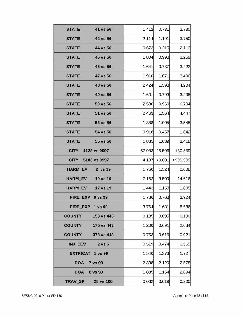
SESUG 2016 Paper SD-130 Appendix Page 38 of 53
STATE 41 vs 56 1.412 0.731 2.730
STATE 42 vs 56 2.114 1.191 3.750
STATE 44 vs 56 0.673 0.215 2.113
STATE 45 vs 56 1.804 0.998 3.259
STATE 46 vs 56 1.641 0.787 3.422
STATE 47 vs 56 1.910 1.071 3.406
STATE 48 vs 56 2.424 1.398 4.204
STATE 49 vs 56 1.601 0.793 3.235
STATE 50 vs 56 2.536 0.960 6.704
STATE 51 vs 56 2.463 1.364 4.447
STATE 53 vs 56 1.888 1.005 3.545
STATE 54 vs 56 0.918 0.457 1.842
STATE 55 vs 56 1.885 1.039 3.418
CITY 1128 vs 9997 67.983 25.596 180.559
CITY 5183 vs 9997 4.187 <0.001 >999.999
HARM_EV 2 vs 19 1.750 1.524 2.008
HARM_EV 10 vs 19 7.162 3.509 14.616
HARM_EV 17 vs 19 1.443 1.153 1.805
FIRE_EXP 0 vs 99 1.736 0.768 3.924
FIRE_EXP 1 vs 99 3.764 1.631 8.686
COUNTY 153 vs 443 0.135 0.095 0.190
COUNTY 175 vs 443 1.200 0.691 2.084
COUNTY 373 vs 443 0.753 0.616 0.921
INJ_SEV 2 vs 6 0.519 0.474 0.569
EXTRICAT 1 vs 99 1.540 1.373 1.727
DOA 7 vs 99 2.338 2.120 2.578
DOA 8 vs 99 1.835 1.164 2.894
TRAV_SP 28 vs 106 0.062 0.019 0.200
SESUG 2016 Paper SD-130 Appendix Page 39 of 53
TRAV_SP 30 vs 106 0.457 0.308 0.678
PERNOTMVIT 1 vs 8 0.007 0.002 0.026
PERNOTMVIT 4 vs 8 0.149 0.041 0.544
PERMVIT 9 vs 50 7.652 6.717 8.717
PERMVIT 17 vs 50 >999.999 <0.001 >999.999
PERMVIT 18 vs 50 42.393 12.446 144.393
PERMVIT 21 vs 50 4.271 3.861 4.726
PERMVIT 23 vs 50 >999.999 <0.001 >999.999
PERMVIT 24 vs 50 101.574 54.747 188.453
PERMVIT 26 vs 50 >999.999 <0.001 >999.999
PERMVIT 33 vs 50 >999.999 <0.001 >999.999
PERMVIT 47 vs 50 >999.999 <0.001 >999.999
PERSONS 8 vs 50 7.772 6.456 9.356
PERSONS 9 vs 50 13.438 10.338 17.467
DRIMP_NONE 0 vs 1 1.388 1.275 1.511
DAMAGE DAMAGE vs TOTAL 0.795 0.706 0.896
DAMAGE MISSING vs TOTAL 7.699 3.471 17.078
SESUG 2016 Paper SD-130 Appendix Page 40 of 53
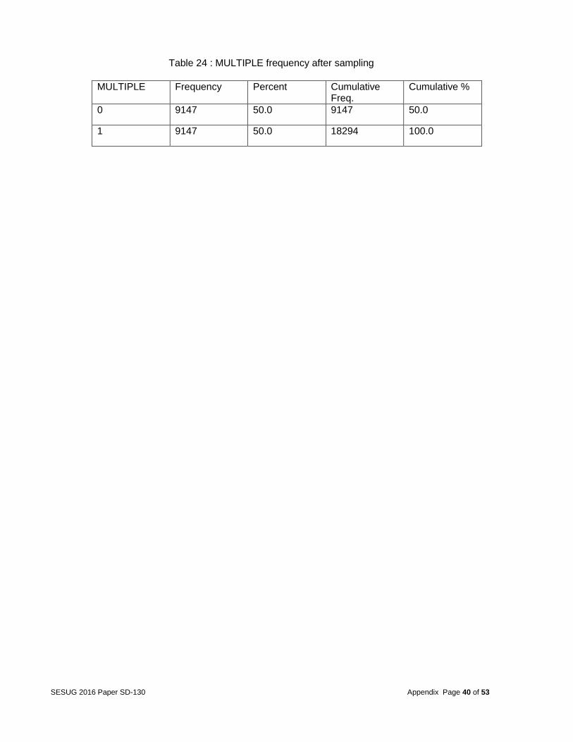
Table 24 : MULTIPLE frequency after sampling
MULTIPLE Frequency Percent Cumulative Freq.
Cumulative %
0 9147 50.0 9147 50.0
1 9147 50.0 18294 100.0
SESUG 2016 Paper SD-130 Appendix Page 41 of 53
Figure 1: FARS Data Base
SESUG 2016 Paper SD-130 Appendix Page 42 of 53
Figure 2: USA map
SESUG 2016 Paper SD-130 Appendix Page 43 of 53
Figure 3: Map of Georgia for years 2012 & 2013
SESUG 2016 Paper SD-130 Appendix Page 44 of 53
Figure 4: Map of North Carolina for years 2012 & 2013
SESUG 2016 Paper SD-130 Appendix Page 45 of 53
Figure 5: Map of California for years 2012 & 2013
SESUG 2016 Paper SD-130 Appendix Page 46 of 53
Figure 6: Map of Wyoming for years 2012 & 2013
SESUG 2016 Paper SD-130 Appendix Page 47 of 53
Figure 7: Histogram of variable VSPD_LIM
SESUG 2016 Paper SD-130 Appendix Page 48 of 53
Figure 8: Flow Chart to Find the Effects of a Variable
SESUG 2016 Paper SD-130 Appendix Page 49 of 53
Figure 9: ROC curves side by side comparison
ROC Curve for Model A ROC Curve for Model B
SESUG 2016 Paper SD-130 Appendix Page 50 of 53
Figure 10: ROC Curve for 2013 Validation Data
Model B – 2013 Data Model A – 2013 Data
SESUG 2016 Paper SD-130 Appendix Page 51 of 53
SAS Code Summary
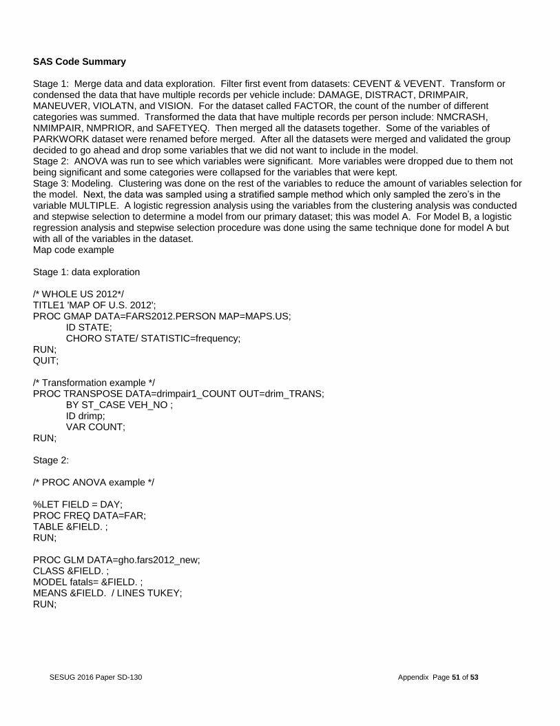
Stage 1: Merge data and data exploration. Filter first event from datasets: CEVENT & VEVENT. Transform or condensed the data that have multiple records per vehicle include: DAMAGE, DISTRACT, DRIMPAIR, MANEUVER, VIOLATN, and VISION. For the dataset called FACTOR, the count of the number of different categories was summed. Transformed the data that have multiple records per person include: NMCRASH, NMIMPAIR, NMPRIOR, and SAFETYEQ. Then merged all the datasets together. Some of the variables of PARKWORK dataset were renamed before merged. After all the datasets were merged and validated the group decided to go ahead and drop some variables that we did not want to include in the model. Stage 2: ANOVA was run to see which variables were significant. More variables were dropped due to them not being significant and some categories were collapsed for the variables that were kept. Stage 3: Modeling. Clustering was done on the rest of the variables to reduce the amount of variables selection for the model. Next, the data was sampled using a stratified sample method which only sampled the zero’s in the variable MULTIPLE. A logistic regression analysis using the variables from the clustering analysis was conducted and stepwise selection to determine a model from our primary dataset; this was model A. For Model B, a logistic regression analysis and stepwise selection procedure was done using the same technique done for model A but with all of the variables in the dataset. Map code example
Stage 1: data exploration /* WHOLE US 2012*/ TITLE1 'MAP OF U.S. 2012'; PROC GMAP DATA=FARS2012.PERSON MAP=MAPS.US; ID STATE; CHORO STATE/ STATISTIC=frequency; RUN; QUIT;
/* Transformation example */ PROC TRANSPOSE DATA=drimpair1_COUNT OUT=drim_TRANS; BY ST_CASE VEH_NO ; ID drimp; VAR COUNT; RUN;
Stage 2:
/* PROC ANOVA example */
%LET FIELD = DAY; PROC FREQ DATA=FAR; TABLE &FIELD. ; RUN;
PROC GLM DATA=gho.fars2012_new; CLASS &FIELD. ; MODEL fatals= &FIELD. ; MEANS &FIELD. / LINES TUKEY; RUN;
SESUG 2016 Paper SD-130 Appendix Page 52 of 53
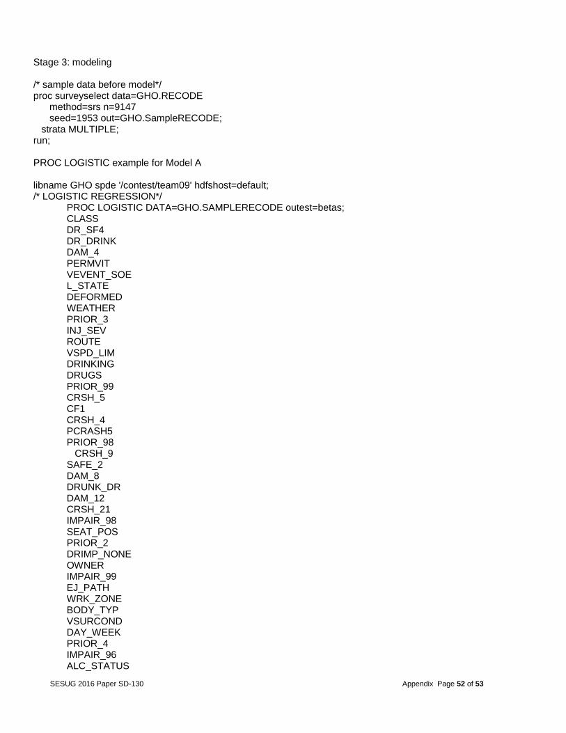
Stage 3: modeling
/* sample data before model*/ proc surveyselect data=GHO.RECODE method=srs n=9147 seed=1953 out=GHO.SampleRECODE; strata MULTIPLE; run;
PROC LOGISTIC example for Model A
libname GHO spde '/contest/team09' hdfshost=default; /* LOGISTIC REGRESSION*/ PROC LOGISTIC DATA=GHO.SAMPLERECODE outest=betas; CLASS
DR_SF4
DR_DRINK
DAM_4
PERMVIT
VEVENT_SOE
L_STATE
DEFORMED
WEATHER
PRIOR_3
INJ_SEV
ROUTE
VSPD_LIM
DRINKING
DRUGS
PRIOR_99
CRSH_5
CF1
CRSH_4
PCRASH5
PRIOR_98
CRSH_9
SAFE_2
DAM_8
DRUNK_DR
DAM_12
CRSH_21
IMPAIR_98
SEAT_POS
PRIOR_2
DRIMP_NONE
OWNER
IMPAIR_99
EJ_PATH
WRK_ZONE
BODY_TYP
VSURCOND
DAY_WEEK
PRIOR_4
IMPAIR_96
ALC_STATUS
SESUG 2016 Paper SD-130 Appendix Page 53 of 53
CRSH_6
CRSH_3
DISTRACT
VEH_SC1
SP_JUR
TYP_INT
PREV_OTH
FUELCODE
;
MODEL MULTIPLE(EVENT='1') =
DR_SF4
DR_DRINK
DAM_4
PERMVIT
VEVENT_SOE
L_STATE
DEFORMED
WEATHER
PRIOR_3
INJ_SEV
ROUTE
VSPD_LIM
DRINKING
DRUGS
PRIOR_99
CRSH_5
CF1
CRSH_4
PCRASH5
PRIOR_98
CRSH_9
SAFE_2
DAM_8
DRUNK_DR
DAM_12
CRSH_21
IMPAIR_98
SEAT_POS
PRIOR_2
DRIMP_NONE
OWNER
IMPAIR_99
EJ_PATH
WRK_ZONE
BODY_TYP
VSURCOND
DAY_WEEK
PRIOR_4
IMPAIR_96
ALC_STATUS
CRSH_6
CRSH_3
SESUG 2016 Paper SD-130 Appendix Page 54 of 53
DISTRACT
VEH_SC1
SP_JUR
TYP_INT
PREV_OTH
HOUR
MINUTE
NOT_HOUR
DISPLACEN
NOT_MIN
AGE
HOSP_HR
HOSP_MN
CITY
LAG_HRS
FUELCODE
/selection=stepwise sle=0.15 sls=0.15 outroc=ROCData ctable ; output out=pred p=phat lower=lcl upper=ucl predprob=(individual crossvalidate) ; score data=gho.samplerecode2013 out=vpred outroc=vroc; roc; roccontrast; run;