face recognition using pca and dct based approach

Face Recognition Using PCA

and DCT Based Approach

Tilak Acharya (109EC0212)

Sunit Kumar Sahoo(109EC0238)

Department of Electronics and Communication Engineering

National Institute of Technology Rourkela

Rourkela- 769008,India

Face Recognition Using PCA

and DCT Based Approach

A project submitted in partial fulfillment of the requirements for the degree of

Bachelor of Technology

in

Electronics and Communication Engineering

by

Tilak Acharya

(Roll 109EC0212)

Sunit Kumar Sahoo

(Roll 109EC0238)

under the supervision of

Prof. Sukadev Meher

Department of Electronics and Communication Engineering

National Institute of Technology Rourkela

Rourkela -769008, India

Electronics and Communication Engineering

National Institute of Technology Rourkela Rourkela-769008, India. www.nitrkl.ac.in

Certificate This is to certify that the thesis titled, “Face Recognition Using PCA and DCT Based

Approach” submitted by Tilak Acharya and Sunit Kumar Sahoo in partial fulfilment of the

requirements for the award of Bachelor of Technology Degree in Electronics and

Communication Engineering at National Institute of Technology, Rourkela (Deemed

University) in an authentic work carried out by them under my supervision and guidance.

Dr. Sukadev Meher Professor

Dept. of Electronics and Communication Engg. National Institute of Technology, Rourkela-769008

Acknowledgment

We would like to express our sincere gratitude and thanks to our supervisor

Prof. Sukadev Meher for for his constant guidance, encouragement and support

throughout the course of this project. We are thankful to Electronics and

Communication Engineering Department to provide us with the unparalleled

facilities throughout the project.We are thankful to Ph.D Scholars for their help

and guidance in completion of the project. We are thankful to our batch mates

and friends Sharad, Siba, Bharat, Swagat, Ritesh for their support and being

such a good company.We extend our gratitude to researchers and scholars

whose papers and thesis have been utilized in our project. Finally, we dedicate

our thesis to our parents for their love, support and encouragement without

which this would not have been possible.

Tilak Acharya Sunit Kumar Sahoo

Abstract Face is a complex multidimensional structure and needs good computing techniques for

recognition. Our approach treats face recognition as a two-dimensional recognition problem.

In this thesis face recognition is done by Principal Component Analysis (PCA) and by

Discrete Cosine Transform (DCT). Face images are projected onto a face space that encodes

best variation among known face images. The face space is defined by eigenface which are

eigenvectors of the set of faces. In the DCT approach we take transform the image into the

frequency domain and extract the feature from it. For feature extraction we use two

approach.. In the 1st approach we take the DCT of the whole image and extract the feature

from it. In the 2nd approach we divide the image into sub-images and take DCT of each of

them and then extract the feature vector from them.

CONTENT

Certificate

Acknowledgement

Abstract

List of figures

List of tables

Chapter 1

Introduction

1.1 Biometrics

1.2 Face recognition

Chapter 2

Principal component analysis

2.1 PCA

2.2 PCA theory

2.3 PCA in face recognition

Chapter 3

Discrete cosine transform

3.1 Introduction

3.2 Definition

3.3 PCA in DCT Domain

3.4 Basic Algorithm For Face Recognition

Chapter 4

Implementation

4.1 PCA

i

ii

iii

vi

vii

1

2

3

4

6

7

7

8

9

13

14

15

16

18

19

20

4.2 DCT

Chapter 5

Results

5.1 Result and analysis

5.2 Average success rate

5.3 Graph of the results

Chapter 6

Conclusion

Bibliography

23

30

31

33

34

37

39

List of figures

Fig:3.1 basic flow chart of DCT

Fig:4.1 few of the images from the database

Fig. 4.2 the image of 10 person in different pose

fig.4.3 mean of the above 40 faces

Fig 4.4 eigenfaces

fig: 4.5sample image

fig:4.6 dct of the image

fig:4.7 histogram equalized version of the DCT

fig:4.8 show the manner in which zigzag scanning is done

Fig: 4.9showing all the elements of the vector

Fig : 4.10showing only the 1st 200 components

Fig: 4.11 shows the division of the whole range of

frequency into three region.

Fig:4.12 shows how a sample image is divided into sub

images DCT transform of the subimages and it histogram

equalized version

List of Tables

Table 5.1: Comparison between different experimental

Results of PCA (1)approach

Table:5.2 Comparison between different experimental

Results of PCA(2) approach

Table 5.3: Comparison between different experimental

Results of DCT approach

National Institute of Technology , Rourkela Page 1

Chapter 1

Introduction


Chapter 1

Introduction

The information age is quickly revolutionizing the way transactions are completed. Human’s

day to day actions are increasingly being handled electronically, instead of face to face or

with pencil and paper. This type of electronic transactions has resulted in a greater demand

for fast and accurate user identification and authentication for establishing proper

communication, access codes for buildings, banks accounts and computer systems for more

secure transactions, PIN's for identification and security. By stealing other’s ATM or any

other smart cards, an unauthorized user can guess the correct personal information. Even after

warnings, many people continue to choose easily guessed PIN’s and passwords e.g.

birthdays, phone numbers and social security numbers, horoscopes. present cases of identity

theft have heightened the need for methods to prove that someone is truly who he/she claims

to be.

Face recognition technology may solve this problem since a face is undeniably connected to

its owner expect in the case of identical twins. It’s non-transferable. The system can then

compare scans to records stored in a central or local database or even on a smart card.


1.1 Biometrics

Biometrics is the technology for automated recognition or verification of the identity of a

person using unique physical or behavioral characteristics such as fingerprints, hand

geometry, iris, face, voice, and signatures. Biometrics is used in the process of authentication

of a person by verifying or identifying that who he, she, or it claims to be, and vice versa. It

uses the property that a human trait associated with a person itself like structure of finger,

face details etc.

Biometrics may be classified into two categories.such as physiological and behavioural.

Physiological biometrics (based on measurements and data derived from direct measurement

of a part of the human body) include:

Finger-scan

Hand-scan

Iris-scan

Facial Recognition

Retina-scan

Behavioral biometrics (based on measurements and data derived from an action) include:

Voice-scan

Signature-scan

Keystroke-scan


A “biometric system” refers to the integrated hardware and software used to conduct

biometric identification or verification.By comparing the existing data with the incoming

data, we can verify the identity of a particular person which has more dynamic effects in the

security and surveliance management, more convenient and easier in fraud detection, better

than password or smart cards.

1.2 Face Recognition

Face is a complex multidimensional structure and needs good computing techniques for

recognition. The face is our primary and first focus of attention in social life playing an

important role in identity of individual. We can recognize a number of faces learned

throughout our lifespan and identify that faces at a glance even after years. There may be

variations in faces due to aging and distractions like beard, glasses or change of hairstyles.

Face recognition is an integral part of biometrics. In biometrics basic traits of human is

matched to the existing data and depending on result of matching identification of a human

being is traced. Face recognition technology analyze the structure, pattern, shape and

positioning of the facial attributes. Eventhough face recognition is very complex technology

it is largely software based. The analysis framework methodology establishes algorithms for

each type of biometric device. Face recognition attempts to find a person in the image by

taking a picture of the person and then facial features are extracted and implemented through

algorithms which are eficient and some modifications are done to improve the existing

algorithm models.


Computers that detect and recognize faces could be applied to a wide variety of practical

applications including criminal identification, security systems, identity verification etc. Face

detection and recognition is used in many places nowadays, in websites hosting images and

social networking sites. Face recognition and detection can be achieved using technologies

related to computer science. Features extracted from a face are processed and compared with

similarly processed faces present in the database. If a face is recognized, it is known or

the system may show a similar face existing in database else it is unknown. In surveillance

system if a unknown face appears more than one time then it is stored in database for further

recognition. These steps are very useful in criminal identification. In general, face recognition

mathematically models the problems in two different ways.in the first method it perform

operation on whole image to get the desired result which is called principal component

analysis. The other one take the image and process it in blocks which is called direct cosine

transform analysis.


Chapter 2

Principal Component Analysis (PCA)


Chapter 2

2.1 Principal Component Analysis (PCA)

Principal component analysis (PCA) was invented in 1901 by Karl Pearson. It is a linear

transformation based on statistical technique. It is used to decrease the dimension of the data

or to reduce the correlation between them. It is a way of identifying patterns present in data,

and expressing the data in such a way that their similarities and differences are highlight.

Since patterns present in data can be hard to find in data of high dimension, where it can not

be represented graphically, PCA is a powerful tool for face detection which is multi-

dimensional.

The purpose of PCA is to reduce the large dimension of data space to a smaller intrinsic

dimension of feature vector (independent variable), which are used to describe the data cost

effectively. The first principal component is the linear combination of the original dimension

along which the variance is maximum. The second principal component is the linear

combination of the original dimension along which the variance is maximum and which is

orthogonal to the first principal component. The n-th principal component is the linear

combination with highest variance , subject to being orthogonal to n-1 principal component.


2.2 PCA THEORY

Principal component analysis in signal processing can be described as a transform of a given

set of n input vectors each of length K formed in the n-dimensional vector x = [x1, x2, ... ,xn]T

into a vector y according to

Each row of x have K variables belonging to one input.

mx represents the mean or expectation of all input variables defined as:

{ }

∑

The matrix A in the above equation is derived from the covariance matrix Cx . Rows of the

matrix A are the eigen vector of the covariance matrix arrange according to the decreasing

order of their eigen value.

The covariance matrix is given by:

{ }

∑

As x is a n dimensional vector so Cx is a nXn vector where each element is given by:

{ }

Rows of A are orthogonal to each other. We choose the number of rows to be present in A,

which is less than or equal to n, and represent the dimension to which we want to reduce y.


2.3 PCA In Face Recognition

The images of the faces we have are in two dimension , let us say of size NXN.

Our aim here is to find the Principal components (also known as Eigen Faces) which can

represent the faces present in the training set in a lower dimensional space.

For all our calculations we need the input data i.e. the faces is a linear form so we map the

NXN image into a 1XN2 vector. Let every linear form of the image in our training set be

represented by In. Let the total no. of faces in the training set be represented as M.

Steps For Computation of the Principal components:

We compute the mean of all the faces vectors :

∑

Next we subtract the mean from the image vector Ii.

We compute the covariance matrix C:

∑

(N

2XN

2 matrix)

Where B = [K1 K2 K3 ……… KM ]T (N

2 X M matrix)

Our next step is to compute the eigen vector of the matrix C or BBT, let it be ui.


But BBT has a very large size and the computation of eigen vector for it is not

practically possible.

So instead we find the eigen vector for the matrix BTB, let vi be the eigen vectors.

BTBvi = livi

Relationship between vi and ui

BTBvi = livi

=> BBTBvi = liAvi

=> CBvi = liBvi

=>Cui =liui where ui = Bvi

So BBT and B

TB have same eigen value and there eigen vector are related by ui = Bvi

The M eigenvalues of BTB (along with their corresponding eigenvectors) correspond

to the M largest eigenvalues of BBT (along with their corresponding eigenvectors).

So now we have the M best eigen vector of C. From that we choose N1 best eigen

vectors i.e. with largest eigen value.

The N1 eigen vector that we have chosen are used as basis to represent the faces. The

eigen vectors should be normalised. The eigen vectors are also referred to as eigen

faces because when it is transformed into a N X N matrix it appears as “ghostly faces”

consisting features of all the training faces.

Representing faces onto this basis:

Each face (minus the mean) Ki in the training set can be represented as a linear

combination of N1 eigenvectors:

∑


wj is the projection of Kj on to the eigen vector uj

So each normalised face Ki can be represented in form of the vector,

Recognising An Unknown Face:

Given an unknown face image (centred and of the same size like the training faces) we follow

these steps to recognise it:

We first convert it to the linear form , I

Then we normalise it by subtracting the mean from it

K = I –mean

Next we project K on all the N1 eigen vectors to obtain the vector W

W = [w1 w2 ….. wN1]T

where

Now we find er = minl ||W-Wl||

Where || || ∑

So er gives the minimum distance the given face has from another face belonging to

the training set. And the given face belongs to that person to whom the face in the

training set belongs.

If the value of er is greater than the threshold T1 but less then threshold T2 then we can

say that it doesn’t belong to any one in the given training set.


If er is greater than threshold T2 we can say that the given image doesn’t belong to

face space and hence is not the image of a face.


Chapter 3

Discrete Cosine Transform (DCT)


Chapter 3

Discrete Cosine Transform (DCT)

3.1 Introduction

A transform is a mathematical operation that when applied to a signal that is being processed

converts it into a different domain and then can be again is converted back to the original

domain by the use of inverse transform.

The transforms gives us a set of coefficients from which we can restore the original samples

of the signal. Some mathematical transforms have the ability to generate decorrelated

coefficients such that most of the signal energy is concentrating in a reduced number of

coefficients.

The Discrete Cosine Transform (DCT) also attempts to decorrelate the image data as other

transforms. After decorrelation each transform coefficient can be encoded independently

without losing compression efficiency. It expresses a finite sequence of data points in terms

of a sum of cosine functions oscillating at different frequencies. The DCT coefficients reflect

different frequency component that are present in it. The first coefficient refers to the

signal’s lowest frequency(DC component) and usually carries the majority of the relevant

information from the original signal. The coefficients present at the end refer to the signal’s

higher frequencies and these generally represent the finer detailed. The rest of the coefficients

carry different information levels of the original signal.


3.2 Definition

Ahmed, Natarajan, and Rao (1974) first introduced the discrete cosine transform (DCT) in

the early seventies. Ever since, the DCT has become very popular, and several versions have

been proposed (Rao and Yip, 1990).

The DCT was categorized by Wang (1984) into four slightly different transformations

named DCT-I, DCT-II, DCT-III, and DCT-IV.

Here we are using only DCT-II and is referred to as DCT and DCT-III as inverse DCT

henceforth.

One dimensional DCT transform is defined as :

∑ (

)

0≤ k ≤ N-1

Where u(n) in the input sequence of length N and its DCT is v(k) and

(0) = √

(k) = √ 1 ≤ k ≤ N-1

The inverse discrete cosine transform permits us to obtain u (n) from v (k). It is defined by:

∑ (

)

0 ≤ n ≤ N-1


In 2 dimension the DCT is defined as :

∑

∑

for u,v = 0,1,2,…,N −1 and α(u) and α(v) are defined above.

Its inverse is given by:

∑

∑

for x,y = 0,1,2,…,N −1.

3.3 PCA IN DCT DOMAIN

In the pattern recognition letter by Weilong Chen, Meng Joo Er , Shiqian Wu it has been

proved that we can apply the PCA directly on the coefficient of Discrete Cosine Transform.

When PCA is applied on a orthogonally transformed version of the original data then the

subspace projection obtained is same as compared to what is obtained by PCA on the

original data. DCT and Block-DCT (it is the process of dividing the images into small blocks

and then taking the DCT of each subimage) are also orthogonal transform, we can apply PCA

on it without any reduction in the performance.


3.4 Basic Algorithm For Face Recognition

The basic Face Recognition Algorithm is discussed below. Both normalization and

recognition are involved in it. The system receives as input an image containing a face .The

normalized (and cropped) face is obtained and then it can be compared with other faces in the

training set, under the same normalised condition conditions like nominal size, orientation

and position. This comparison is done by comparing the features extracted using the DCT.

The basic idea here is to compute the DCT of the normalized face and retain a certain subset

of the DCT coefficients as a feature vector describing this face.

Fig:3.1 basic flow chart of DCT


This feature vector contains the mostly low and mid frequency DCT coefficients, as these are

the ones that have maximum information contain and highest variance.

The feature vector which we obtain is still a very large in dimension. From the above

discussion we know that PCA can be used in DCT domain without any change in the

principal component. So we use the technique of PCA discussed in the previous section for

reducing the dimensionality of the feature vector.

Once we have defined the face space with the help of Eigen vectors , then we can find the

projection of the feature vectors in that space.

The projection of the input face and the projection of the faces in the data base are compared

by finding out the Euclidean distance between them. A match is obtained by minimising the

Euclidean distance.


Chapter 4

Implementation


Chapter 4

Implementation

4.1 PCA

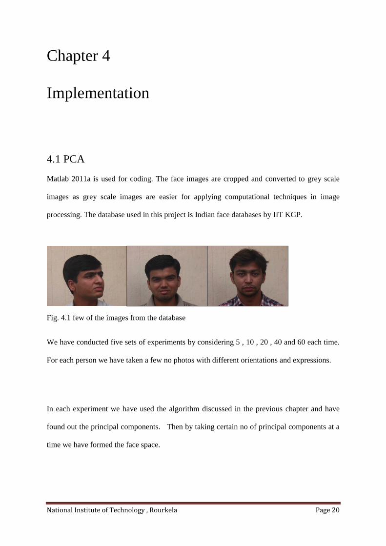
Matlab 2011a is used for coding. The face images are cropped and converted to grey scale

images as grey scale images are easier for applying computational techniques in image

processing. The database used in this project is Indian face databases by IIT KGP.

Fig. 4.1 few of the images from the database

We have conducted five sets of experiments by considering 5 , 10 , 20 , 40 and 60 each time.

For each person we have taken a few no photos with different orientations and expressions.

In each experiment we have used the algorithm discussed in the previous chapter and have

found out the principal components. Then by taking certain no of principal components at a

time we have formed the face space.


Fig. 4.2 Shows the image of 10 person in different pose

fig.4.3 mean of the above 40 faces


After the face space is formed we take a unknown face from the data base, normalize it by

subtracting the mean from it .

Then we project it on the eigen vectors and derive its corresponding components.

Next we evaluate the Euclidian distance from the feature vector of other faces and find the

face to which it has minimum distance. WE classify the unknown image to belong to that

class (provided the minimum distance is less than the defined threshold).

Fig 4.4 eigenfaces


4.2 DCT

We have used Matlab 2011a is used for implementation. We use the same data base as the

above case. The face images are cropped and changed grey level. Next we convert the image

to DCT domain for feature extraction. The feature vector is dimensionally much less as

compared to the original image but contains the required information for recognition.

The DCT of the image has the same size as the original image. But the coefficients with

large magnitude are mainly located in the upper left corner of the DCT matrix.

Low frequency coefficients are related to illumination variation and smooth regions (like

forehead cheek etc.) of the face. High frequency coefficients represent noise and detailed

information about the edijes in the image. The mid frequency region coefficients represent

the general structure of the face in the image.

Hence we can’t ignore all the low frequency components for achieving illumination

invariance and also we can’t truncate all the high frequency components for removing noise

as they are responsible for edges and finer details.

Here we are going to consider two approach for feature extraction:

i. Holistic approach (we take the DCT of the whole image)


ii. Block wise approach (we divide the image into small sub-images and take their DCT)

In holistic approach we take the DCT of the whole image and extract the feature vector from

it. In block wise approach we divide the image into many sub-images and then take DCT of

each of them. We extract the feature vector from each of them and concatenate then to form

the final feature vector.

HOLISTIC APPROACH

We take DCT of the image. Here our image size is 480 x 480. Next we convert the DCT of

the image into a one dimensional vector by zigzag scanning. We do a zigzag scanning so that

in the vector the components are arranged according to increasing value of frequency.

fig: 4.5sample image fig:4.6 dct of the

image

fig:4.7 histogram equalized

version of the DCT


fig:4.8 show the manner in which zigzag scanning is

done

From the plot of the vector we observe that the low- frequency components have high

magnitude high frequency component have very less magnitude (i.e. much less than 1).

Fig: 4.9showing all the elements of the vector


Fig : 4.10showing only the 1st 200 components

Now we divide the whole range of frequency into three equal sections and derive the

coefficient of feature vector from each section.

In case of low frequency section we reject the 1st three terms and consider the next 800 terms.

We reject the 1st three terms to achieve illumination invariance.

Fig: 4.11it shows the division of the whole range of frequency into three region.


In case of mid and high frequency section we find the position where the components with

high value generally occur. We find this by comparing the images of the DCT of the images

in the training set. Once the position whose values are to be considered are fixed then we

obtain the coefficient from those position and include them in the feature vector. Here in our

case we are considering 100 coefficient from each section.

So for each image we have obtained a feature vector of size 1000.

Next we apply PCA on these feature vector and find the corresponding eigen vector as

discussed in the previous section.

We select the dimension according to our requirement and represent the feature vector in that

space.

When we get a unknown face we first find its corresponding feature vector . Then we project

the feature vector to the space described above. next we find the face to which it has

minimum Euclidian distance and classify it accordingly.


BLOCK DCT APPROACH

In this approach we divide the image into small blocks. Then we extract the feature vector

from each block and combine them to get our required feature vector.We should choose the

block size optimally. If it is too small then two adjacent blocks wouldn’t be uncorrelated and

it would give rise to redundant features. And if the block size is too high then we may miss

out some feature.

Here we are considering block size of 32 x 32 pixels. So the original image is divided into

225 sub-images. Then we take the DCT of each sub image . So each DCT of sub-image

contain 1024 coefficients.

From this we remove the DC component and then take the next 20 elements by scanning in a

zigzag manner.

Fig:4.12 shows how a sample image is divided into sub images

DCT transform of the subimages and it histogram equalized version


Next we normalise the image we obtain from each sub-image and combine then to get our

feature vector.

The feature vector obtained is still quite large, so we use PCA on the feature vector and

obtain the eigen vector.

We select the dimension according to our requirement and represent the feature vector in that

space.

When we get a unknown face we first find its corresponding feature vector . Then we project

the feature vector to the space described above. next we find the face to which it has

minimum Euclidian distance and classify it accordingly.


Chapter 5

Results


Chapter 5

Results

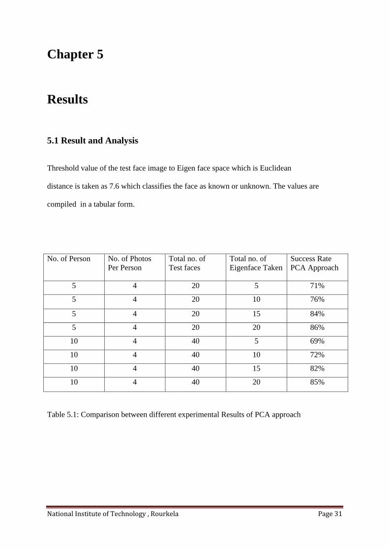
5.1 Result and Analysis

Threshold value of the test face image to Eigen face space which is Euclidean

distance is taken as 7.6 which classifies the face as known or unknown. The values are

compiled in a tabular form.

No. of Person No. of Photos

Per Person

Total no. of

Test faces

Total no. of

Eigenface Taken

Success Rate

PCA Approach

5 4 20 5 71%

5 4 20 10 76%

5 4 20 15 84%

5 4 20 20 86%

10 4 40 5 69%

10 4 40 10 72%

10 4 40 15 82%

10 4 40 20 85%

Table 5.1: Comparison between different experimental Results of PCA approach


No. of Person No. of Photos

Per Person

Total no. of

Test faces

Total no. of

Eigenface Taken

Success Rate

PCA Approach

20 8 160 10 67%

20 8 160 15 70%

20 8 160 20 75%

40 8 320 10 63%

40 8 320 15 69%

40 8 320 20 73%

60 8 480 10 55%

60 8 480 15 63%

60 8 480 20 70%

Table:5.2 Comparison between different experimental Results of PCA approach

No. of Person No. of Photos Per

Person

Total no. of Test

faces

Total no. of

Eigenface Taken

Success Rate DCT BLOCK-DCT

5 8 40 10 80% 82%

5 8 40 15 85% 85%

5 8 40 20 88% 90%

10 8 80 10 76% 78%

10 8 80 15 82% 83%

10 8 80 20 85% 86%

20 8 160 10 72% 74%

20 8 160 15 75% 76%

20 8 160 20 80% 80%

Table 5.3: Comparison between different experimental Results of DCT approach


Four different images for each mentioned condition were taken to test for five and ten

different people. Light intensity is tried to keep low. Size variation of a test image is not

altered to much extent. We can observe that normal expressions are recognized as face

efficiently because facial features are not changed much in that case and in other cases where

facial features are changed efficiency is reduced in recognition.similarly the results shows

poor performances for lesser eigenfaces.

5.2 Average Success Rate

(71+ 76+ 84+ 86+ 69 + 72+82+85)/8 = 78.125% for PCA

(80+85+88+76+82+85+72+75+80)/9 = 80.333% for DCT

(82+85+90+78+83+86+74+76+80)/9 = 81.556% for Block-DCT

However, this efficiency cannot be generalized as it is performed on less number

of test of images and conditions under which tested may be changed on other time.


5.3 Graph of the Result

Series 1 : No. of Person Series 2 No. of Photos Per Person

Series 3: Total no. of Test faces Series 4: Total no. of Eigenface Taken

Series 5: Success Rate

0

10

20

30

40

50

60

70

80

90

100

1 2 3 4 5 6 7 8

Series1

Series2

Series3

Series4

Series5


series 1:Total no f faces series 2: success rate in PCA

0

10

20

30

40

50

60

70

80

90

100

1 2 3 4 5 6 7 8 9

Series1

Series2


series 1:dct success rate series 2: block dct success rate

0%

1000%

2000%

3000%

4000%

5000%

6000%

7000%

8000%

9000%

10000%

1 2 3 4 5 6 7 8 9

Series1

Series2


Chapter 6

Conclusion


Chapter 6

Conclusion

In this thesis we implemented the face recognition system using Principal Component

Analysis and DCT based approach. The system successfully recognized the human faces and

worked better in different conditions of face orientation upto a tolerable limit. But in PCA, it

suffers from Background (deemphasize the outside of the face, e.g., by multiplying the input

image by a 2D Gaussian window centered on the face), Lighting conditions (performance

degrades with light changes),Scale (performance decreases quickly with changes to the head

size), Orientation (perfomance decreases but not as fast as with scale changes).

In block DCT based approach our the results are quite satisfactory.but it suffers from it’s

problem that all images should align themselves in the centre position minimizing the

skewness of the image to lower level.


Bibliography

[1] Application of DCT Blocks with Principal Component Analysis for Face

Recognition Proceedings of the 5th WSEAS Int. Conf. on SIGNAL, SPEECH and

IMAGE PROCESSING, Corfu, Greece, August 17-19, 2005 (pp107-111)

[2] PCA and LDA in DCT domain ,Weilong Chen, Meng Joo Er *, Shiqian Wu Pattern

Recognition Letters 26 (2005) 2474–2482

[3] Rafael Gonzalez and Richard Woods. Digital Image Processing. Addison Wesley, 1992.

[4] Eigenfaces for Face Detection/Recognition,M. Turk and A. Pentland, "Eigenfaces for

Recognition", Journal of Cognitive Neuroscience, vol. 3, no. 1, pp. 71-86, 1991

[5] M. A. Turk and A. P. Pentland. Face recognition using eigenfaces. In IEEE Computer

Society,Conference on Computer Vision and Pattern Recognition, CVPR 91, pages (586 -

591, 1991.)

[6] Face Recognition using Block-Based DCT Feature Extraction ,K Manikantan1, Vaishnavi

Govindarajan1,V V S Sasi Kiran1, S Ramachandran2 Journal of Advanced Computer

Science and Technology, 1 (4) (2012) 266-283

[7] http://www.face-rec.org

face recognition using pca and dct based approach

Documents