face alignment in-the-wild: a survey - arxiv · face alignment in-the-wild: a survey xin jina,b,...
TRANSCRIPT
Face Alignment In-the-Wild: A Survey
Xin Jina,b, Xiaoyang Tana,b,∗
aDepartment of Computer Science and Engineering, Nanjing University of Aeronautics and Astronautics, #29Yudao Street, Nanjing 210016, P.R. China
bCollaborative Innovation Center of Novel Software Technology and Industrialization, Nanjing University ofAeronautics and Astronautics, Nanjing 210016, China
Abstract
Over the last two decades, face alignment or localizing fiducial facial points has received increasing
attention owing to its comprehensive applications in automatic face analysis. However, such a
task has proven extremely challenging in unconstrained environments due to many confounding
factors, such as pose, occlusions, expression and illumination. While numerous techniques have
been developed to address these challenges, this problem is still far away from being solved. In
this survey, we present an up-to-date critical review of the existing literatures on face alignment,
focusing on those methods addressing overall difficulties and challenges of this topic under uncon-
trolled conditions. Specifically, we categorize existing face alignment techniques, present detailed
descriptions of the prominent algorithms within each category, and discuss their advantages and
disadvantages. Furthermore, we organize special discussions on the practical aspects of face align-
ment in-the-wild, towards the development of a robust face alignment system. In addition, we
show performance statistics of the state of the art, and conclude this paper with several promising
directions for future research.
Keywords: Face alignment, Active appearance model, Constrained local model, Cascaded
regression, Deep convolutional neural networks.
1. Introduction
Fiducial facial points refer to the predefined landmarks on a face graph, which are mainly
located around or centered at the facial components such as eyes, mouth, nose and chin (see Fig.
1). Localizing these facial points, which is also known as face alignment, has recently received
significant attention in computer vision, especially during the last decade. At least two reasons
account for this. Firstly, many important tasks, such as face recognition, face tracking, facial
expression recognition, head pose estimation, can benefit from precise facial point localization.
∗Corresponding author: Tel.: +86-25-8489-6490/6491 (Ext 12106 ) (O); fax: +86-25-8489-2452; E-mail:[email protected].
Preprint submitted to Computer Vision and Image Understanding August 16, 2016
arX
iv:1
608.
0418
8v1
[cs
.CV
] 1
5 A
ug 2
016
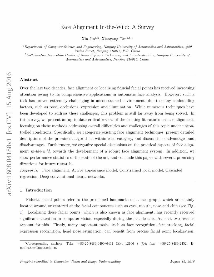
Figure 1: Illustration of some example face images with 68 manually annotated points from the IBUG database [4].
Secondly, although some level of success has been achieved in recent years, face alignment in
unconstrained environments is so challenging that it remains an open problem in computer vision,
and continues to attract researchers to attack it.
While face detection is generally regarded as the starting point for all face analysis tasks [1], face
alignment can be regarded as an important and essential intermediary step for many subsequent
face analyses that range from biometric recognition to mental state understanding. Concrete tasks
may differ in the number and type of the needed facial points, as well as the way these points are
used. Below we give some details on three typical tasks where face alignment plays a prominent
role:
• Face recognition: Face alignment is widely used by face recognition algorithms to improve
their robustness against pose variations. For example, in the stage of face registration, the
first step is usually to locate some major facial points and use them as anchor points for
affine warping, while other face recognition algorithms, such as feature-based (structural)
matching [2, 3], rely on accurate face alignment to build the correspondence among local
features (e.g, eyes, nose, mouth, etc.) to be matched.
• Attribute computing: Face alignment is also beneficial to facial attribute computing, since
many facial attributes such as eyeglasses and nose shape are closely related to specific spatial
positions of a face. In [5], six facial points are localized to compute qualitative attributes
and similes that are then used for robust face verification in unconstrained conditions.
• Expression recognition: The configurations of facial points (typically between 20-60) are
reliable indicative of the deformations caused by expressions, and the subsequent analysis
will reveal the particular type of expression that may lead to such deformation. Many works
[6, 7, 8, 9, 10] follow this idea and use various features extracted from these points for
expression recognition.
The above-mentioned applications, as well as numerous ones yet to be conceived, urge the need
for developing robust and accurate face alignment techniques in real-life scenarios.
Under constrained environments or on less challenging databases, the problem of face align-
ment has been well addressed, and some algorithms even achieve performance that is close to that
2

(a) Pose (b) Occlusion (c) Expression (d) Illumination
Figure 2: An illustration of the great challenges of face alignment in the wild (IBUG [4]), from left to right (everytwo columns): variations in pose, occlusion, expression and illumination.
of human beings [11, 12]. Under unconstrained conditions, however, this task is extremely chal-
lenging and far from being solved, due to the high degree of facial appearance variability caused
either by intrinsic dynamic features of the facial components such as eyes and mouth, or by am-
bient environment changes. In particular, the following factors have significant influence on facial
appearance and the states of local facial features:
• Pose: The appearance of local facial features differ greatly between different camera-object
poses (e.g., frontal, profile, upside down), and some facial components such as the one side
of the face contour, can even be completely occluded in a profile face.
• Occlusion: For face images captured in unconstrained conditions, occlusion frequently hap-
pens and brings great challenges to face alignment. For example, the eyes may be occluded
by hair, sunglasses, or myopia glasses with black frames.
• Expression: Some local facial features such as eyes and mouth are sensitive to the change
of various expressions. For example, laughing may cause the eyes to close completely, and
largely deform the shape of the mouth.
• Illumination: Lighting (varying in spectra, source distribution, and intensity), may signif-
icantly change the appearance of the whole face, and make the detailed textures of some
facial components missing.
These challenges are illustrated in Fig. 2 by the IBUG database [4]. An ideal face alignment system
should be robust to these facial variations on one hand; while on the other hand, as efficient as
possible to satisfy the need of practical applications (e.g., real-time face tracking).
Over the last two decades, numerous techniques have been developed for face alignment with
varying degrees of success. Celiktutan et al. [13] surveyed many traditional methods for face
3

alignment of both 2D and 3D faces, but some recent state-of-the-art methods are not covered.
Wang et al. [14] gave a more comprehensive survey of face alignment methods over the last two
decades, but the overall difficulties and challenges in unconstrained environments have not been
highlighted. More recently, Yang et al. [15] provided an empirical study of recent face alignment
methods, aiming to draw some empirical yet useful conclusions and make insightful suggestions
for practical applications.
The significant contribution of this paper is to give a comprehensive and critical survey of the
ad hoc face alignment methods addressing the difficulties and challenges in unconstrained environ-
ments, which we believe would be a useful complement to [13, 14, 15]. To be self-contained, some
traditional methods for face alignment covered in [13, 14] are also included. However, contrary to
the previous works, we pay special attention to study and summarize the motivation and successful
experiences behind the state-of-the-art, expecting to offer some insights into the studies of this
field. Furthermore, we organize special discussions on the practical aspects of constructing a face
alignment system, including training data augmentation, face preprocessing, shape initialization,
accuracy and efficiency tradeoffs. This in our opinion is a very important topic in practice, but
is mostly ignored in previous studies. In addition, we show comparative performance statistics of
the state of the art, and propose several promising directions for future research.
In the following Section 2, we briefly describe the main idea of face alignment and categorize
existing methods into two main categories. Then, the prominent methods within each category
are reviewed and analyzed in Section 3 and 4. In Section 5, we investigate some practical aspects
of developing of a robust face alignment system. In Section 6, we discuss a few issues concerning
performance evaluation. Finally, we conclude this paper with a discussion of several promising
directions for further research in Section 7.
2. Overview
The problem of face alignment has a long history in computer vision, and a large number
of approaches have been proposed to tackle it with varying degrees of success. From an overall
perspective, face alignment can be formulated as a problem of searching over a face image for
the pre-defined facial points (also called face shape), which typically starts from a coarse initial
shape, and proceeds by refining the shape estimate step by step until convergence. During the
search process, two different sources of information are typically used: facial appearance and
shape information. The latter aims to explicitly model the spatial relations between the locations
of facial points to ensure that the estimated facial points can form a valid face shape. Although
some methods make no explicit use of the shape information, it is common to combine these two
sources of information.
4

Table 1: Categorization of the popular approaches for face alignment.Approach Representative works
Generative methodsActive appearance models (AAMs)
Regression-based fitting Original AAM [16]; Boosted Appearance Model [17]; Nonlinear discriminative ap-proach [18]; Accurate regression procedures for AMMs [19]
Gradient descent-based fitting Project-out inverse compositional (POIC) algorithm [20]; Simultaneous inverse com-positional (SIC) algorithm [21]; Fast AAM [22]; 2.5D AAM [23]; Active OrientationModels [24]
Part-based generative deformable models Original Active Shape Model (ASM) [25]; Gauss-Newton deformable part model [26];Project-out cascaded regression [27]; Active pictorial structures [28]
Discriminative methodsConstrained local models (CLMs)a
PCA shape model Regularized landmark mean-shift [29]; Regression voting-based shape model matching[30]; Robust response map fitting [31]; Constrained local neural field [32]
Exemplar shape model Consensus of exemplar [11]; Exemplar-based graph matching [33]; Robust Discrimi-native Hough Voting [34]
Other shape models Gaussian Process Latent Variable Model [35]; Component-based discriminative search[36]; Deep face shape model [37]
Constrained local regression Boosted regression and graph model [38]; Local evidence aggregation for regression[39]; Guided unsupervised learning for model specific models [40]
Deformable part models (DPMs) Tree structured part model [41]; Structured output SVM [42]; Optimized part model[43]; Regressive Tree Structured Model [44]
Ensemble regression-voting Conditional regression forests [12]; Privileged information-based conditional regressionforest [45]; Sieving regression forest votes[46]; Nonparametric context modeling [47]
Cascaded regressionTwo-level boosted regression Explicit shape regression [48]; Robust cascaded pose regression [49]; Ensemble of
regression trees [50]; Gaussian process regression trees [51];Cascaded linear regression Supervised descent method [52]; Multiple hypotheses-based regression [53]; Local bi-
nary feature [54]; Incremental face alignment [55]; Coarse-to-fine shape search [56]Deep neural networksb
Deep CNNs Deep convolutional network cascade [57]; Tasks-constrained deep convolutional net-work [58]; Deep Cascaded Regression[59]
Other deep networks Coarse-to-fine Auto-encoder Networks (CFAN) [60]; Deep face shape model [37]a Classic Constrained Local Models (CLMs) typically refer to the combination of local detector for each facial point and the parametric Point Distribution
Model [61, 62, 29]. Here we extend the range of CLMs by including some methods based on other shape models (i.e., exemplar-based model [11]). Inparticular, we will show that the exemplar-based method [11] can also be interpreted under the conventional CLM framework.
b We note that some deep learning-based systems can also be placed in other categories. For instance, some systems are constructed in a cascade manner[60, 59, 63], and hence can be naturally categorized as cascaded regression. However, to highlight the increasing important role of deep learningtechniques for face alignment, we organize them together for more systematic introduction and summarization.
Before describing specific and prominent algorithms, a clear and high-level categorization will
help to provide a holistic understanding of the commonality and differences of existing methods
in using the appearance and shape information. For this, we follow the basic modeling principles
in pattern recognition, and roughly divide existing methods into two categories: generative and
discriminative.
• Generative methods: These methods build generative models for both the face shape and
appearance. They typically formulate face alignment as an optimization problem to find the
shape and appearance parameters that generate an appearance model instance giving best
fit to the test face. Note that the facial appearance can be represented either by the whole
(warped) face, or by the local image patches centered at the facial points.
• Discriminative methods: These methods directly infer the target location from the facial
appearance. This is typically done by learning independent local detector or regressor for
each facial point and employing a global shape model to regularize their predictions, or by
5

directly learning a vectorial regression function to infer the whole face shape, during which
the shape constraint is implicitly encoded.
Table 1 summarizes algorithms and representative works for face alignment, where we fur-
ther divide the generative methods and discriminative methods into several subcategories. A few
methods overlap category boundaries, and are discussed at the end of the section where they are
introduced. Below, we discuss the motivation and general approach of each category first, and
then, give the review of prominent algorithms within each category, discussing their advantages
and disadvantages.
3. Generative methods
Typically, faces are modelled as deformable objects which can vary in terms of shape and
appearance. Generative methods for face alignment construct parametric models for facial ap-
pearance similar to EigenFace [64], but differ from EigenFace in that they take into account the
deformation of face shape, and build appearance model in a canonical reference frame where the
shape variations have been removed. Fitting a generative model aims to find the shape and ap-
pearance parameters that can generate a model instance fitting best to the test face.
According to the type of facial representation, generative methods can be further divided into
two categories: Active Appearance Models (AAMs) that use the holistic representations, and
part-based generative deformable models that use part-based representation.
3.1. Active appearance models
Active Appearance Models (AAMs), proposed by Cootes et al. [16], are linear statistical
models of both the shape and the appearance of the deformable object. They are able to generate
a variety of instances by a small number of model parameters, and therefore have been widely
used in many computer vision tasks, such as face recognition [65], object tracking [66] and medical
image analysis [67]. In the field of face alignment, AAMs are arguably the most well-known family
of generative methods that have been extensively studied during the last 15 years [16, 20, 21, 22].
In the following, we first briefly introduce the basic AAM algorithm including AAM modeling
and fitting, then summarize and analysis some recent advances on AAM research, and finally
present some discussions about the advantages and disadvantages of AAMs.
3.1.1. Basic AAM algorithm: modeling and fitting
In the section, we briefly introduce the basic AAM algorithm: modeling and fitting. Note that
we do not intend to give a very comprehensive and detailed overview of the basic AAM algorithm,
and refer the reader to recent surveys [68, 14] for more details.
6

AAM modeling. An AAM is defined by three components, i.e., shape model, appearance model,
and motion model. The shape model, which is coined Point Distribution Model (PDM) [69], is
built from a collection of manually annotated facial points s = (xT1 , ...,x
TN)T describing the face
shape, where xi = (xi, yi) is the 2-D location of the ith point. To learn the shape model, the
training face shapes are normalized with respect to a global similarity transform (typically using
Procrustes Analysis [70]) and Principal Component Analysis (PCA) is applied to obtained a set
of linear shape bases. The shape model can be mathematically expressed as:
s(p) = s0 + Sp, (1)
where s0 ∈ R{2N,1} is the mean shape, S ∈ R{2N,n} and p ∈ Rn is the shape eigenvectors and
parameters. Furthermore, this shape model need to be composed with a 2D global similarity
transform, in order to position a particular shape model instance arbitrarily on the image frame.
For this, using the re-orthonormalization procedure described in [20], the final expression for the
shape model can be compactly written using 1 by appending S with 4 similarity eigenvectors.
The appearance model is obtained by warping the training faces onto a common reference
frame (typically defined by the mean shape), and applying PCA onto the warped appearances.
Mathematically, the texture model is defined as follows:
A(c) = a0 + Ac, (2)
where a0 ∈ R{F,1} is the mean appearance, A ∈ R{F,m} and c ∈ R{m,1} is the appearance eigen-
vectors and parameters respectively.
To produce the shape-free textures, the motion model plays a role as a bridge between the
image frame and the canonical reference frame. Typically, it is a warp function W that defines
how, given a shape, the image should be warped into a canonical reference frame. Popular motion
models include piece-wise affine warp [20, 22] and Thin-Plate Splines warp [71].
AAM fitting. Given an test image I, AAM fitting aims to find the optimal parameters p and c
so that the synthesized appearance model instance gives best fit to the test image in the reference
frame. Formally, let I[p] = I(W(p)) denote the vectorized version of the warped test image, then
AAM fitting can be formulated as the following optimization problem,
arg minp,c||I[p]− a0 −Ac||2. (3)
Solving 3 is an iterative process that at each iteration an update of the current model parameters
is estimated. In general, there are two main approaches for AAM fitting.
The first approach is to assume a fixed relationship between the residual image and the model
7
parameter increments, and learn it via regression. For example, in the original AAM paper [72], this
relationship is assumed linear and learned by linear regression, while in [18] a nonlinear repressor
is learned via boosting. However, because the basic assumption that the regression functions are
fixed is incorrect [20], the regression-based fitting strategies are efficient but approximate.
The second approach is to employ a standard gradient descend algorithm. But unfortunately,
standard gradient descend algorithms are inefficient when applied to AAMs fitting. Matthews et al.
[20] addressed this problem with a so-called project-out inverse compositional algorithm (POIC)
algorithm, which decouples shape from appearance by projecting out appearance variation, and
estimates the warp update in the model coordinate frame and then compose it inversely to the
current warp. Although POIC is extremely fast, it is also known to have a small convergence radius,
i.e., convergence is especially bad when training and testing images differ strongly [21]. Different
from POIC that projects out the appearance variations, the simultaneous inverse compositional
(SIC) algorithm [73] optimizes the shape parameter and appearance parameter simultaneously
under the inverse compositional framework. SIC has been shown to be more robust than POIC
for generic AAM fitting, but the computational cost is much higher [21]. Besides SIC, another
accurate AAM fitting algorithm is the Alternating Inverse Compositional (AIC) algorithm [74],
which solves two separate minimization problems, one for the shape and one for the appearance
optimal parameters, in an alternating fashion.
3.1.2. Recent advances on AAMs
Recently, some extensions and improvements of AAMs have been proposed to make this classic
algorithm better adapted to the task of face alignment in-the-wild. In general, recent advances
on AAMs mainly focus on three aspects: (1) unconstrained training data [22], (2) robust image
representations [75, 76] and (3) robust and fast fitting strategies [75, 22].
Unconstrained training data. Although some AAM fitting algorithms (e.g., the Simultane-
ous Inverse Compositional (SIC) algorithm [73]) are known to perform well on constrained face
databases, their performance has not been assessed on in-the-wild databases until recently. Tz-
imiropoulos et al. [22] showed that, when trained in-the-wild, AAMs perform notably well and in
some cases comparably with current state-of-the-art methods, without using sophisticated shape
priors, robust features or robust norms. Fig. 3 shows a fitting case and the reconstruction of the
image, produced by AAM built in the wild [22].
Robust image representations. Typically, AAMs use the pixel-based image representation
that is sensitive to global lighting [72, 20, 22], and a natural way to improve the robustness of
AAMs is to use the feature-based representation. In general, robust image features, such as HOG
[77], SIFT [78] or SURF [79] that describe distinctive and important image characteristics, can
generalize better to unseen images. Some recent works have confirmed the robustness of the
8

Note that the cost for calculating Hffw as above is n2N andcomes from the first term (this is because ATJI ∈ Rm×n).An additional cost for the forward additive formulation isthat ∂W
∂p is evaluated at p and not at p = 0, but the cost fordoing this can be negligible.
An interesting observation following the above analysisis that, for both forward and inverse algorithms, the domi-nant computational cost comes from projecting out the ap-pearance subspace when calculating the Hessian. If wechoose not to do this, then the total cost is further reducedto (n2 + m)N . Note however that, in this case, the result-ing algorithms are approximate and not exact. We leave theevaluation of these approximate algorithms as interestingfuture work.
5. Fitting AAMs in-the-wildSimultaneous AAM fitting algorithms are known to per-
form well but their performance has not been previously as-sessed on recently collected in-the-wild data sets. In thissection and in the one that follows, we aim to address thisgap in literature. In particular, we show that AAMs performalmost comparably to some state-of-the-art face alignmentalgorithms, even without using any priors (the fitting algo-rithms described above are used as is) and using raw pixelintensities as features.
One reason for not evaluating AAMs in-the-wild is thatSIC as proposed in [16] is too slow to be employed, espe-cially for m � n, which is the case for generic face align-ment. However, as we showed above, the cost per iterationfor Fast-SIC and Fast-Forward is on the order of a few timesmN . This cost can be easily handled by current systemspossibly allowing a close to real-time implementation.
Another reason for ruling out AAMs from unconstrainedface alignment experiments is the fact that AAMs are notconsidered robust. All optimization problems considered inthe previous sections are least-squares problems, and as itis well-known in computer vision least-squares combinedwith pixel intensities as features typically results in poorperformance for data corrupted by outliers (e.g. sunglasses,occlusions, difficult illumination). Standard ways of deal-ing with outliers are robust features and robust norms. Theproblem with feature extraction is that it might slow downthe speed of the fitting algorithm significantly especiallywhen the dimensionality of the featured-based appearancemodel is large. The problem with robust norms is that scaleparameters must be estimated (or percentage of outlier pix-els must be predefined) and this task is not trivial.
We propose a third orthogonal direction for fitting AAMsin unconstrained conditions which is via training AAMs in-the-wild. In fact, this paper is one of the few that proposethe combination of generative models plus training in-the-wild (plus robust optimization for model fitting). It turns outthat this combination is very beneficial for unconstrained
(a) (b)
Figure 2. (a) A face image from the test set of LFPW [3]. Theimage was not seen during training. Landmarks were detected byfitting the AAM using the Fast-SIC algorithm. (b) Reconstruc-tion of the image from the appearance subspace. The appearancesubspace is powerful because the AAM was built in the wild.
AAM fitting. Consider for example the image shown inFig. 2 (a). This is a test image from the LFPW data set.This image was not seen during training, but similar imagesof unconstrained nature were used to train the shape andappearance model of an AAM. Fig. 2 (b) shows the recon-struction of the image from the appearance subspace. Aswe may see the appearance model is powerful enough to re-construct the texture almost perfectly. Fitting with a robustalgorithm (Fast-SIC in this case) gives the fitting result ofFig. 2 (a). This example illustrates why the results of thenext section should not be considered too surprising.
6. ResultsThe main target of our experiments was not to prove that
AAM fitting is state-of-the-art in face alignment but to showthat robust fitting plus training in-the-wild improves AAMfitting performance dramatically. For this reason, we did notattempt to use sophisticated shape priors for regularization,nor we employed robust features/appearance models or ro-bust norms for improving performance. In all experiments,we used simple pixel intensities as features. Additionally,we note that we did not attempt to reproduce the results ofany of current state-of-the-art methods because their imple-mentation is not trivial and in most cases the code is notpublicly available. Instead, we report the performance ofAAMs using two very popular error measures and we re-fer the readers to these papers and the references therein fordrawing comparisons with the algorithms described in thispaper.
To facilitate fitting, we used a multi-resolution fittingapproach with m = 50, n = 3 at the lowest level andm = 200, n = 10 at the highest. We found experimen-tally, that for robust fitting, m should be at least one or-der of magnitude greater than n. Note that in most AAMpapers, m and n are chosen so that a fixed percentage ofvariance is fixed (most cases 95%). This may result in rel-atively large model sizes that are more difficult to optimize.Instead we chose the model parameters by running the al-
Figure 3: (a) A face image from the test set of LFPW [11], with facial points detected by the Fast-SIC algorithmproposed in [22]. (b) Reconstruction of the image from the appearance subspace. (Fig. 2 in [22])
appearance model built upon feature-based representation [75, 24, 80].
Robust and fast fitting strategies. It is widely acknowledged that the Project-out Inverse
Compositional (POIC) algorithm is fast but has a small convergence radius, while the Simultaneous
Inverse Compositional (SIC) algorithm is accurate but very slow. Due to this, some recent advances
on AAMs have focused on robust and fast fitting algorithms. For example, it was found in [75, 80]
that the Alternating Inverse Compositional (AIC) algorithm [74] performs well for generic AAM
fitting. Although AIC is slower than the project-out algorithm, it is still very fast probably allowing
a real-time implementation. Furthermore, by using a standard results from optimization theory,
Tzimiropoulos et al. [22] dramatically reduced the dominant cost for both SIC and the standard
Lukas-Kanade algorithm, making both algorithms very attractive speed-wise for practical AAM
systems.
3.1.3. Discussion
We have described the basic AAM algorithm and recent advances on AAMs. Despite the
popularity and success, AMMs have been traditionally criticized for the limited representational
power of their holistic representation, especially when used in wild conditions. However, recent
works on AAMs [75, 76, 81] suggest that this limitation might have been over-stressed in the
literature and that AAMs can produce highly accurate results if appropriate training data [22],
image representations [75, 76] and fitting strategies [75, 22] are employed.
Despite this, AAMs are still considered to have the following drawbacks: (1) Since the holistic
appearance model is used, partial occlusions cannot be easily handled. (2) For the appearance
model built in-the-wild, the dimension of appearance parameter is very high, which makes AAMs
difficult to optimize and likely to converge to undesirable local minima. One possible way to
overcome these drawbacks is to use part-based representations, due to the observation that local
features are generally not as sensitive as global features to lighting and occlusion. In the following
section, we turn to part-based generative methods.
9

3.2. Part-based generative deformable models
Part-based generative methods build generative appearance models for facial parts, typically
with a shape model to govern the deformations of the face shapes. In this paper, we do not
distinguish the specific form of the shape model, and refer to all part-based generative methods
collectively as part-based generative deformable models.
In general, there are two approaches to construct generative part models. The first is to
construct individual appearance model for each facial part. A notable example is the well-known
original Active Shape Models [69, 25] that combine the generative appearance model for each facial
part and the Point Distribution Model for global shapes. However, we note that a more natural
and popular way is to model individual facial part is the discriminatively trained local detector
[82, 29, 30, 31], as adopted by a very successful family of methods coined Constrained Local Models
(CLMs) [29, 31]. Actually, ASMs can be regarded as the predecessors of CLMs, because they are
similar in both the models and the fitting process. Therefore, we refer the reader to Section 4.1
for more details about ASMs under the CLM framework.
The second approach is to construct generative models for all facial parts simultaneously. For
example, one can concatenate all facial parts (image patches) to form a part-based representa-
tion for the whole face, and then build generative appearance model for it. The Gauss-Newton
Deformable Part Model (GN-DPM) [26] has explored this idea, and build linear statistical model
for both the concatenated facial parts and the shape using PCA. Benefiting from the part-based
representation, the motion model of GN-DPM degenerates to similarity transformation, rather
than the affine warp of AAMs. In the fitting phase, GN-DPM formulate and solve the non-linear
least squares optimization problem similar to AAMs [20, 22]. The part-based appearance model
along with a global shape model is optimized by the fast SIC algorithm [22] in a Gauss-Newton
fashion. Extensive experiments on wild face databases [83, 84, 41] demonstrate that the part-based
GN-DPM outperforms AAMs by a large margin.
While GN-DPM employs the inverse compositional fitting algorithm, Tzimiropoulos et al. [27]
consider the forward algorithm for the non-linear least square optimization problem akin to that
of GN-DPM. Although analytic gradient decent method is employed in [27], it is only used for
the derivation of the learning and fitting basis of the proposed Project-Out Cascaded Regression
(PO-CR) method. In particular, PO-CR learns from data a sequence of averaged Jacobians and
descent directions via regression in a subspace orthogonal to the facial appearance variation. Apart
from the PCA-based appearance model in GN-DPM and PO-CR, Antonakos et al. [28] propose to
model the appearance of facial parts using multiple pairwise distributions based on the edges of a
graph (GMRF), and show that this outperforms the commonly used PCA model under an inverse
Gauss-Newton optimization framework.
Compared to AAMs, the part-based generative deformable models mainly have the advantages
10

from part-based representation, i.e., more robust to global lighting and occlusion in wild conditions.
As shown in [26], part-based generative models may have the same representational power of AAMs,
but are easier to optimize. That is, when the initial shape is far from the ground truth, part-based
generative deformable models are more likely to get converged to a good solution, although the
formulation is non-convex by nature.
3.3. Summary and discussion
We have reviewed generative methods for face alignment in two categories, i.e., Active Appear-
ance Models (AAMs) that use the holistic representation and the part-based generative deformable
models that use the part-based representation. In general, the fitting result of a generative ap-
pearance model to a test image typically depends on two factors: (1) the representational power
of the model, and (2) the difficulty in optimizing the model. As investigated in [26], when trained
in-the-wild, both AAMs and part-based generative deformable models can reconstruct the appear-
ance of an unseen image well, but the part-based generative deformable models are considered to
be easier to optimize than AAMs. Furthermore, recent results show that if unconstrained training
data [22], robust image representations [75, 76] and appropriate fitting strategies [75, 22, 26, 27] are
employed, generative methods can produce a very high degree of fitting accuracy for face alignment
in-the-wild. These results suggest that the limitations of generative methods, especially the AAMs,
might have been over-stressed in the literature. In addition, generative methods typically have the
advantage of requiring fewer training examples than the discriminative methods to perform well
[28].
However, with recent development of unconstrained facial databases with an abundance of
annotated facial data captured, the discriminative methods, which are capable of effectively lever-
aging large bodies of training data, are arguably now playing a more and more prominent role in
face alignment in-the-wild. Next, we will turn to discriminative methods.
4. Discriminative methods
Discriminative face alignment methods seek to learn a (or a set of) discriminative function that
directly maps the facial appearance to the target facial points. In general, there are two main
lines of research for discriminative methods. The first line is to follow the “divide and conquer”
strategy by learning discriminative local appearance model (detector or regressor) for each facial
point, and a shape model to impose global constraints on these local models. This line can be
further subdivided into three classes: (1) Constrained Local Models (CLMs) that learn independent
local detector for each facial point, with a shape model to regularize the detection responses of these
local detectors. (2) constrained local regression methods that learn independent local regressor for
each point and use a graph model to guide the search of these local regressors, and (3) deformable
11

Table 2: Overview of the six classes of discriminative methods in our taxonomy.Appearance model Shape model Highlights of the method
Constrained local models Independently trained localdetector that computes apseudo probability of the tar-get point occurring at a par-ticular position.
Point DistributionMoldel; Exemplarmodel, etca.
The local detectors are first correlated withthe image to yield a filter response for eachfacial point, and then shape optimization isperformed over these filter responses.
Constrained local regression Independently trained localregressor that predicts a dis-tance vector relating to apatch location.
Markov RandomFields to model therelations betweenrelative positions ofpairs of points.
Graph model is used to constrain the searchspace of local regressors by exploiting theconstellations that facial points can form.
Deformable part models Part-based appearance modelthat computes the appearanceevidence for placing a tem-plate for a facial part.
Tree-structured mod-els that are easier tooptimize than densegraph structures.
All parameters of the appearance model andshape model are discriminatively learned ina max-margin structured prediction frame-work; efficient dynamic programming algo-rithms can be used to find globally optimalsolutions.
Ensemble regression-voting Image patches to cast votesfor all facial points relating tothe patch centers;Local appearance featurescentered at facial points.
Implicit shape con-straint that is natu-rally encoded into themulti-output function(e.g., regression tree).
Votes from different regions are ensembled toform a robust prediction for the face shape.
Cascaded regression Shape-indexed feature that isrelated to current shape esti-mate (e.g., concatenated im-age patches centered at the fa-cial points).
Implicit shape con-straint that is natu-rally encoded into theregressor in a cas-caded learning frame-work.
Cascaded regression typically starts from aninitial shape (e.g., mean shape), and re-fines the holistic shape through sequentiallytrained regressors.
Deep neural networks Whole face region that is typ-ically used to estimate thewhole face shape jointly;Shape-indexed featureb.
Implicit shape con-straint that is en-coded into the net-works since all facialpoints are predictedsimultaneously.
Deep network is a good choice to model thenonlinear relationship between the facial ap-pearance and the shape update.Among others, deep CNNs have the capac-ity to learn highly discriminative features forface alignment.
a Constrained Local Models (CLMs) typically employ a parametric (PCA-based) shape model [29], but we will show that the exemplar-based method [11]can also be derived from the CLM framework. Furthermore, we extend the range of CLMs by including some methods that combine independently localdetector and other face shape model [35, 36, 37].
b Some deep network-based systems follow the cascaded regression framework, and use the shape-indexed feature [60].
part models that learn the local appearance model and the tree structured shape model jointly in
a discriminative framework.
The second line is to directly learn a vectorial regression function to infer the whole face shape,
during which the shape constraint is implicitly encoded. This line can also be further subdivided
into three classes: (1) ensemble regression-voting methods that cast votes for all facial points
from local regions via regression, and ensemble the votes from different regions to form a robust
prediction, (2) cascaded regression methods that learn a vectorial regression function in a cascade
manner to estimate the face shape stage-by-stage, and (3) deep neural networks that employ deep
convolutional networks [57, 58] or auto-encoder networks [60] to model the nonlinear relationship
between the facial appearance and the shape update.
Table 2 gives a overview of the six classes of discriminative methods in our taxonomy, where
12

the appearance model, shape model and highlights of them are listed respectively to show the
differences and relations between them.
4.1. Constrained local models
Constrained Local Models (CLMs), which can date back to the seminal work of Active Shape
Model (ASM) [25], are a relatively mature approach for face alignment [61, 29, 30, 31, 32]. In
the training phase, CLMs learn independent local detector for each facial point, and a prior shape
model to characterize the deformation of face shapes. In testing, face alignment is typically for-
mulated as an optimization problem to find the best fit of the shape model to the test image. We
classify CLMs as the discriminative methods because of the discriminative nature of usual local
detectors.
While the seminal work of [29] unifies various CLM approaches in a probabilistic framework,
it only focuses on the CLMs using the Point Distribution Model (PDM). However, we note that
some methods using other shape model (i.e., the exemplar shape model [11]) are also close to
[29] in methodology. Hence, in this paper we refer to those methods combining independent local
detector and any kind of shape model collectively as Constrained Local Models1.
In the following, we will first briefly introduce the basic Point Distribution Model (PDM) based
CLM algorithm including modeling and fitting, then summarize and analysis recent advances on
CLMs in handling unconstrained challenges. In particular, we will show that exemplar-based
method [11] can also be interpreted under the conventional CLM framework [29]. Finally, we
discuss the advantages and disadvantages of CLMs.
4.1.1. Basic CLM algorithm: modeling and fitting
In this section, we will briefly describe the basic CLM algorithm building upon the Point
Distribution Model (PDM), which has two procedures: modeling and fitting.
CLM modeling. A CLM consists of two important components: local detector for each facial
point, and the shape model that captures the deformations of valid face shapes. The task of local
detector is to compute a pseudo probability (likelihood) that the target point occurs at a particular
position. Existing local detectors can be broadly categorized into three groups.
• Generative approach: Generative approaches can be use to model local image patches cen-
tered at the annotated facial points. For example, [69, 86] assume that the local appearance
1A disadvantage of our extended definition for CLMs is that, the classical Deformable Part Models (DPMs)with the tree structured shape model [85, 41] will also be covered by our definition of CLMs, which however aretraditionally treated as an independent approach relative to others. In this paper, we will still treat DPMs as anindependent group of methods in face alignment, and describe them in Section 4.3
13

is multivariate Gaussian distributed, and use the Mahalanobis distance as the fitting response
for a new image patch.
• Discriminative classifier: Discriminative classifier-based approach learns a binary classifier
for each point with annotated image patches to discriminate whether the target point is
aligned or not when testing. To cast various CLM fitting strategies in a unified probabilistic
framework, the output of these classifiers are typically transformed into pseudo probabilities.
Different types of classifiers have been exploited in literature, e.g., logistic regression [29],
SVM [11, 31], and Local Neural Field (LNF) [32].
• Regression-voting approach: The regression-voting approach casts votes for the target point
from a nearby region, then compute the pseudo probabilities by accumulating votes from
different regions [82, 30]. The regression-voting approach has the potential to be more efficient
since a locally exhaustive search is avoided.
Due to the local patch support and large variations in training, the local detectors are typically
imperfect, and the correct location will not always be at the location with the highest detection
response. To address this drawback, a global shape model is typically employed to regularize the
detection of these local detectors. For this, conventional CLMs use the Point Distribution Model
(PDM) that simply models the normalized face shapes as multivariate Gaussian and approximates
them using PCA (see Equation 1).
CLM fitting. Overall, give an image I, the goal of PDM-based CLMs is to find the optimal shape
parameter p that maximizes the probability of its points corresponding to consistent locations
of the facial features. By assuming that the local search of each facial point is conditionally
independent, the fitting objective of PDM-based CLMs can be written as:
p∗ = arg maxp
p(p|{li =1}Ni=1, I)
= arg maxp
p(p)N∏
i=1
p(li =1|xi(p), I),(4)
where xi(p) is the location of the ith point generated by the shape model, li ∈ {1,−1} is a discrete
random variable denoting whether the ith facial point is aligned or not, and p(p) is the prior
distribution of p that can be estimated from the training data.
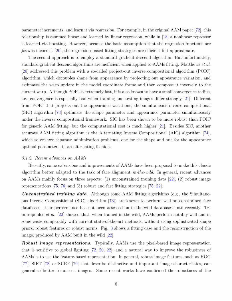
CLM fitting based on 4 is an iterative process (see Fig. 4) that entails (1) convolving the
local detectors with the image to generate response maps, and (2) performing a global shape
optimization procedure over these response maps. To make optimization efficient and numerically
stable, a common choice of existing optimization strategies is to replace the true response maps
14
202 Int J Comput Vis (2011) 91: 200–215
over all landmarks, regularized appropriately:
Q(p) = R(p) +n∑
i=1
Di (xi;I), (2)
where R penalizes complex deformations (i.e. the regular-ization term) and Di denotes the measure of misalignmentfor the ith landmark at xi in the image I (i.e. the data term).The form of regularization is related to the assumed distribu-tion of PDM parameters describing plausible object shapes,common examples of which include the Gaussian (Bassoet al. 2003) and Gaussian mixture model (GMM) (Gu andKanade 2008) estimates. Examples of the misalignment er-ror functions include the Mahalanobis distance over localpatch appearance (Cootes and Taylor 1992) and the boostedHarr-like feature based classifier (Cristinacce and Cootes2006).
Although it is possible to utilize general purpose op-timization strategies to minimize (2), this is rarely donein practice. With the exception of tracking-targeted ap-proaches, where Di is often chosen as the least squares dif-ference between the template and the image (Zhou et al.2005), most variants of CLM fitting employ a specializedfitting strategy. One reason for this is that the misalignmenterror functions typically exhibit significant noise in the spa-tial domain of xi . As such, local deterministic optimizationstrategies, such as the Newton method, are often unstable.Stochastic optimization strategies, such as the simplex basedmethod used in Cristinacce and Cootes (2004), are morestable since they do not make use of gradient information,which renders them somewhat insensitive to measurementnoise. However, convergence may be slow when using theseoptimizers, especially for a complex PDM with a large num-ber of parameters.
Since a landmark’s misalignment error depends onlyon its spatial coordinates, an independent exhaustive localsearch for the location of each landmark can be performedefficiently (i.e. at all integer pixel locations around the es-timated landmark locations). Therefore, most CLM variantsimplement a two step fitting strategy, where an exhaustivelocal search is first performed to obtain a response map foreach landmark. Optimization is then performed over theseresponse maps, which admit more sophisticated strategiescompared to generic optimization methods that make no useof domain specific knowledge. An illustration of this twostep procedure is presented in Fig. 2. It should be noted thatthis is made possible by the restricted search domains for{xi}ni=1, a condition specific to CLM’s formulation. A de-tailed discussion of such strategies is presented in Sect. 2.2.
2.1.2 A Probabilistic Interpretation
The CLM objective in (2) can be interpreted as maximiz-ing the likelihood of the model parameters such that all of
Fig. 2 Illustration of CLM fitting and its two components: (i) an ex-haustive local search for feature locations to get the response maps{p(li = 1|x,I)}ni=1, and (ii) an optimization strategy to maximize theresponses of the PDM constrained landmarks
its landmarks are aligned with their corresponding locationson the object in an image. The specific form of the objec-tive implicitly assumes conditional independence betweendetections for each landmark, the probabilistic interpretationof which takes the form:
p(p|{li = 1}ni=1,I) ∝ p(p)
n∏
i=1
p(li = 1|xi ,I), (3)
where li ∈ {1,−1} is a discrete random variable denotingwether the ith landmark is aligned or misaligned. With thisformulation, the regularization and misalignment error func-tions in (2) take the following forms:
R(p) = − ln{p(p)} (4)
Di (xi;I) = − ln{p(li = 1|xi ,I)}. (5)
To clarify exposition in the following sections, let us ex-plicate the specific forms of the prior and likelihood in (3)utilized in this work. We model the likelihood of alignmentat a particular landmark location, x, as follows:
p(li = 1|x,I) = 1
1 + exp{liCi (x;I)} , (6)
where Ci denotes a classifier that discriminates aligned frommisaligned locations. Notice that this likelihood is a properprobability mass function since it is non-negative every-where, and:
p(li = 1|x,I) + p(li = −1|x,I) = 1. (7)
For the classifier Ci we use the logistic regressor (Wang et al.2008a):
Ci (x;I) = wTi P(W(x;I)) + bi, (8)
where {wi , bi} respectively denote the gain and bias, andP(c) normalizes c to zero mean and unit variance. Here,W(x;I) is an image patch:
W(x;I) = [I(z1); . . . ;I(zP )]; {zi}Pi=1 ∈ �x, (9)
Figure 4: Illustration of PDM-based CLM fitting and its two components: (1) an exhaustive local search for featurelocations to get the response maps {p(li = 1|x, I)}Ni=1 and (2) an optimization strategy to maximize the responsesof the PDM constrained facial points. (Fig. 2 in [29])
with some approximate forms and then perform Guass-Newton optimization over them instead of
the original response maps.
Table 3: Different approximation strategies of response map.Approximation of response map
Isotropic Gaussian estimator [25] N (xi(p);µi, σ2i I
(e))Anisotropic Gaussian estimator [62] N (xi(p);µi,Σi)
Gaussian mixture model [87]∑Ki
k=1 πikN (xi(p);µik,Σik)Gaussian kernel estimation [29]
∑yj∈Ψxi
πyjN (xi(p); yj , ρ
2I(e))
The seminal framework of [29] unifies various approximation strategies for the true response
maps. As listed in Table 3, they are (1) the isotropic Gaussian estimators used by original ASMs
[69, 25], where µi is the the location of the maximum filter response within the ith response
map, and σ−2i is the detection confidence over peak response coordinate, (2) a full covariance
anisotropic Gaussian estimators used in [62], where Σi is the anisotropic covariance matrix of
Gaussian distribution, (3) Gaussian mixture model (GMM) used in [87], where Ki denotes the
number of modes and {πik}Kik=1 are the mixing coefficients for the GMM of the ith point, and (4)
a homoscedastic isotropic Gaussian kernel estimation (KDE) used by [29], where πyj= p(li =
1|yj, I) denotes the likelihood that the ith point is aligned at location yj, and ρ2 denotes the
variance of the noise on facial point locations, I(e) is the identity matrix. Among them, the
nonparametric Gaussian kernel estimation (KDE) method [29] is considered to achieve a good
tradeoff between representation power and the computational complexity. This method is known
as Regularized Landmark Mean-Shift (RLMS) fitting, as the resulting update equations based on
this nonparametric approximation are reminiscent of the well known mean-shift [88] over the facial
point but with regularization imposed by the Point Distribution Model.
Due to its effectiveness and efficiency, the RLMS method [29] has been extensively investigated.
For example, Baltruvsaitis et al. [89] explored the information of depth images, and extend the
RLMS [29] algorithm to a 3D vision. Unlike aforementioned approximations to response maps,
15

[31] proposes a novel discriminative regression based approach to directly estimate the parameter
update, and results in significant performance improvement.
4.1.2. Recent advances on CLMs
Recently, some improvements of the conventional CLMs have been proposed to better handle
various challenges in-the-wild. In general, recent advances on CLMs mainly focus on three aspects:
(1) better local detectors, (2) discriminative fitting, and (3) other shape models.
Better local detectors. Conventional CLMs typically use logistic regression [29] or SVM [11, 31]
to train local detector, which however is plagued by the problem of ambiguity, especially on the
wild databases. To mitigate this ambiguity, some advanced local detectors have been proposed,
such as the Minimum Output Sum of Squared Errors (MOSSE) filters [90] and the Local Neural
Field (LNF) patch expert, which are able to capture more complex information and exploit spatial
relationships between pixels, and hence can achieve better detection results.
Discriminative fitting. It is widely acknowledged that the formulation based on CLMs is non-
convex, and in general prone to local minima. As an alternative, Asthana et al. [31] proposed a
novel Discriminative Response Map Fitting (DRMF) method for the CLM fitting that outperforms
the RLMS fitting method [29] in wild databases. We conjecture that the robustness of DRMF
mainly stems from the discriminative training process, which can effectively leverage large bodies
of training data.
Other shape models. One problem with the Point Distribution Model (PDM) is that its the
model flexibility is heuristically determined by PCA dimension. To overcome this drawback, some
other shape models are proposed to combine with the local detectors for face alignment [35, 11, 37].
In particular, we will show that the exemplar-based method [11] can be derived and well interpreted
under the conventional CLM framework [29].
The exemplar-based method [11] assumes that the face shape s = (x1, ...,xN)T in the test image
is generated by one of the transformed exemplar shapes (global models). Let sk,t (k = 1, ..., D)
denote locations of all facial points in the kth of the D exemplars that transformed by some
similarity transformation t, and let xi,k,t denote location of the ith facial point of the transformed
exemplar sk,t. By assuming that conditioned on the global model sk,t, the location of each facial
point xi is conditionally independent of one another, the exemplar-based shape model p(s) can be
written as follows:
p(s) =D∑
k=1
∫
t∈Tp(s, sk,t)dt
=D∑
k=1
∫
t∈T
N∏
i=1
p(xi|xi,k,t)p(sk,t)dt,
(5)
16

where p(xi|xi,k,t) is modeled as a Gaussian distribution centered at xi,k,t, and the prior of the global
model p(sk,t) is assumed as an uniform distribution. Then, by replacing the shape model p(p) in
conventional CLM framework 4 with above exemplar-based model p(s), we derive the objective
function of [11] (difference in notations) as follows:
s∗=arg maxs
D∑
k=1
∫
t∈T
N∏
i=1
p(xi|xi,k,t)p(li =1|xi, I)dt. (6)
This function is optimized by employing RANSAC to sample global models. Due to the use
of RANSAC, the exemplar-based method [11] has two advantages over conventional CLMs: (1)
independent of shape initialization, and (2) robust to partial occlusion, and achieves excellent
performance on the wild LFPW database [11].
The global models in [11] are scored and selected by the global likelihood, i.e., multiplying
the detection response of each local detector. However, as pointed by Jin et al. [34], this global
likelihood score function ignores the difference between local detectors, while in fact, an eye detector
is typically more reliable than a chin detector. In [34], a discriminatively trained score function
is proposed to evaluate the goodness of a global model, which weighs the importance of different
local detectors. Furthermore, an efficient pipeline was proposed in [34] to alleviate the effect of
inaccurate anchor points for generating global models.
4.1.3. Discussion
We have reviewed the basic CLM algorithm and recent advances. In general, CLMs are con-
sidered to be more robust to partial occlusion and global lighting than the holistic approaches
(e.g., AAMs) [29], due to their part-based modeling. However, the local detectors of CLMs are
imperfect and have been shown to result in detection ambiguities in testing. Furthermore, since
the global shape optimization is performed on the response maps, the detection ambiguities may
lead to performance bottleneck, when facing various challenges in unconstrained conditions.
Another disadvantage of CLMs is that they perform an expensive locally exhaustive search for
each facial point. One way to reduce the computational cost is to use a displacement expert (local
regressor, i.e., estimate the relative position of the target point with respect to the given patch.
We will turn to this topic in the next section.
4.2. Constrained local regression
Besides the CLMs, another local model-based approach is to train independent local regressor
for each point, and employ a global shape model to restrict the search of these local regressors to
anthropomorphically consistent regions [38, 39]. Since this idea is similar to CLMs, we refer to
this approach as constrained local regression.
17

A representative work of this group is the Boosted Regression coupled with Markov Netwroks
[38] (BoRMaN) method, which iteratively uses Support Vector Regressoin (SVR) to provide an
initial prediction for all points, and then applies the Markov Network to ensure that the new
locations sampled to apply the local regressors are from correct point constellations. BoRMaN
let each node in the graph associated to a spatial relation between two points and define pairwise
relations between nodes, which allows a representation that is invariant to in-plane rotations, scale
changes and translations. Essentially, BoRMaN performs an iterative sequential refinement of
the estimate, where the previous target estimate becomes the test location at the next iteration.
Martinez et al. [39] argue that this sequential estimation approach has a series of drawbacks, for
example, sensitive to the starting point and any errors in the estimation process. To improve the
robustness of BoRMaN, [39] propose to detect the target location by aggregating the estimates
obtained from stochastically selected local appearance information into a single robust prediction,
and refer to their algorithm as Local Evidence Aggregated Regression (LEAR).
The main advantage of constrained local regression approach is that combing local regressors
with MRF may drastically reduce the time needed to search for point location, while its disad-
vantages are: (1) similar to CLMs, its performance is limited by the detection ambiguities of the
independently trained local regressors, and (2) globally optimizing MRF is intractable. An alter-
native choice to the graph-based MRF are the tree-structured models, which are also effective to
capture global elastic deformation, but easier to optimize than MRF.
4.3. Deformable part models
The tree-structured models are a natural and effective choice to model deformable objects
[85, 41], which benefit from the existence of an efficient dynamic programming algorithms [91] for
finding globally optimal solutions. Actually, discriminatively trained tree-structured models have
been successfully explored in many computer vision tasks, such as object detection [92], human
pose estimation [85], and recently in face alignment [41, 42, 44]. We follow the nomenclature of
[92] and refer to them collectively as deformable part models (DPMs).
The main challenges of applying tree-structured model for face alignment may lie in the fact
that a single tree-structured pictorial structure, perhaps, is insufficient to capture various shape
deformations due to viewpoint. This problem is addressed by the seminal work of Zhu et al. [41],
with a unified framework for face detection, pose estimation and face alignment. They modeled
every facial point as a part and used mixtures of trees to capture the global topological changes due
to viewpoint; a part will only be visible in certain mixtures/views. Formally, let Tm = (Vm, Em)
be a linearly-parameterized, tree-structured pictorial structure for the mth mixture. Then, given
18

image I and a face shape s = (x1, ...,xN)T , the tree structured part model of view m scores s as:
S(I, s,m) = Appm(I, s) + Shapem(s) + αm
Appm(I, s) =∑
i∈Vmwm
i ·φ(I,xi)
Shapem(s) =∑
ij∈Emamijdx
2+bmijdx+cmijdy2+dmijdy,
(7)
where Appm(I, s) sums the appearance evidence at each part in s, Shapem(s) scores the mixture-
specific spatial arrangement of s, and αm is a scalar bias associated with view point mixture m.
Since parts may look consistent across some changes in viewpoint, [41] allows different mixtures
to share part templates to reduce the computational complexity.
To learn above mixtures of tree structured part models, the Chow-Liu algorithm [93] is first
used to find the maximum likelihood tree structure that best explains the face shape for a given
mixture. Then, for each view, all the model parameters in Eq. 7 is discriminatively learned in a
max-margin structured prediction framework. In the testing phase, the input image is scored by
all tree structures Tm = (Vm, Em) respectively, and the globally optimal shape s is efficiently solved
with dynamic programming algorithm [91].
Due to its simplicity and effectiveness, the tree structured part model [41] has been extensively
investigated and improved for face alignment. Uricar et al. [94] argue that the learning algorithm
of [41] is a variant of a two-class Support Vector Machines, which optimizes the detection rate of
resulting face detector while the facial point locations serve only as latent variables not appearing
in the loss function. In contrast, Uricar et al. [94] directly optimizes the average face alignment
error with a novel objective function using the Structured Output SVMs algoirthm, which leads
to a significant improvement in alignment accuracy. Yu et al. [43] presented a two-stage cascaded
deformable shape model for face alignment, where a group sparse learning method is proposed to
automatically select the optimized anchor points to achieve robust initialization based on the part
mixture model of [41]. Hsu et al. [44] proposed to improve the run-time speed and localization
accuracy of [41] with the Regressive Tree Structure Model (RTSM), where the tree structured
model is applied on images with increasing resolution.
In general, the tree structured part model is effective at capturing global elastic deformation,
while being easy to optimize unlike dense graph structure. Furthermore, it provide an unified
framework to solve three tasks, namely face detection, face alignment and pose estimation, which
is very appealing in automatic face analysis. However, its sluggish runtime impedes the potential
for real-time facial point tracking; and perhaps due to the fact that the tree-based shape models
allow for the non-face like structures to occur frequently, the performance of the tree structured
part model [41] is reported to be slightly inferior to that of the CLMs [29, 31].
19

A common limitation of above part-based discriminative methods (i.e., CLMs, constrained local
regression, and DPMs), however, is that their performance is greatly constrained by the ambiguity
of the local appearance models. To break this bottleneck, many researchers have proposed to jointly
estimate the whole face shape from the image, as described in the following sections.
4.4. Ensemble regression-voting
Apart from above local appearance model-based methods, another main stream of discrimi-
native methods is to jointly estimate the whole face shape from image, during which the shape
constraint is implicitly exploited. A simple way for this is to cast votes for the face shape from
image patches via regression. Since voting from a single region is rather weak, a robust prediction
is typically obtained by ensembling votes from different regions. We refer to these methods as en-
semble regression-voting. In general, the choice of the regression function, which can cast accurate
votes for all facial points, is the key factor of the ensemble regression-voting approach.
Regression forests [95] are a natural choice to perform regression-voting due to their simplicity
and low computational complexity. Cootes et al. [30] use random forest regression-voting to
produce accurate response map for each facial point, which is then combined with the CLM fitting
for robust prediction. Dantone et al. [12] pointed out that conventional regression forests may
lead to a bias to the mean face, because a regression forest is trained with image patches on the
entire training set and averages the spatial distributions over all trees in the forest. Therefore,
they extended the concept of regression forests to conditional regression forests. A conditional
regression forest consists of multiple forests that are trained on a subset of the training data
specified by global face properties (e.g., head pose used in [12]). During testing, the head pose is
first estimated by a specialized regression forest, then trees of the various conditional forests are
selected to estimate the facial points. Due to the high efficiency of random forests, [12] achieves
close-to-human accuracy while processing images in real-time on the Labeled Faces in the wild
(LFW) database [96]. After that, Yang et al. [45] extended [12] by exploiting the information
provided by global properties to improve the quality of decision trees, and later deployed a cascade
of sieves to refine the voting map obtained from random regression forests [46]. Apart from the
regression forests [12, 97, 45, 46], Smith et al. [47] used each local feature surrounding the facial
point to cast a weighted vote to predict facial point locations in a nonparametric manner, where
the weight is pre-computed to take into account the feature’s discriminative power.
In general, the ensemble regression-voting approach is more robust than previous local detector-
based methods, and we conjecture that this robustness mainly stems from the combination of votes
from different regions. However, current ensemble regression-voting approach, arguably, have not
achieved a good balance between accuracy and efficiency for face alignment in-the-wild. The
random forests approach [12, 97, 45, 46] is very efficient but can hardly cast precise votes for those
20

unstable facial points (e.g., face contour), while on the other hand, the nonparametric feature
voting approach based on facial part features [47] is more accurate but suffers from very high
computational burden. To pursue a face alignment algorithm that is both accurate and efficient,
much research has focused on the cascaded regression approach as described in the next section.
4.5. Cascaded regression
Recently, cascaded regression has established itself as one of the most popular and state-of-
the-art methods for face alignment, due to its high accuracy and speed [48, 57, 52, 54, 56]. The
motivation behind this approach is that, since performing regression from image features to face
shape in one step is extremely challenging, we can divide the regression process into stages, by
learning a cascade of vectorial regressors.
Formally, given an image I and an initial shape s0, the face shape s is progressively refined by
estimating a shape increment ∆s stage-by-stage. In a generic form, a shape increment ∆s at stage
t is regressed as:
∆st = Rt(Φt(I, st−1)
), (8)
where st−1 is the shape estimated in the previous stage, Φt is the feature mapping function, and
Rt is the stage regressor. Note that Φt(I, st−1) is referred to as shape-indexed feature [48, 49]
that depends on the current shape estimate, and can be either designed by hand [52, 56] or by
learning [48, 54, 50]. In the training phase, the stage regressors (R1, ...,RT ) are sequentially learnt
to reduce the alignment errors on training set, during which geometric constraints among points
are implicitly encoded.
(a) (b) (c) (d) (e) (f)
Figure 1. A selected prediction result on the 300-W dataset using cGPRT. The shape estimate is initialized and iteratively updated througha cascade of regression trees: (a) initial shape estimate, (b)–(f) shape estimates at different stages of cGPRT.
matrix is then learned by minimizing the squared loss func-tion with l2 regularization, known as Ridge regression [12].
Instead of using gradient boosting, we propose cas-cade Gaussian process regression trees (cGPRT) that canbe incorporated as a learning method for a CRT predictionframework. Gaussian process regression (GPR) is known togive good generalization [16] but high computational com-plexity. By using a special kernel leading to low computa-tional complexity in prediction, cGPRT provides good gen-eralization compared with the CRT within the same pre-diction time. The proposed cGPRT is formed by a cas-cade of Gaussian process regression trees (GPRT), and eachGPRT considers a kernel function that is defined by a setof trees. The kernel measures the similarity between twoinputs based on the number of trees where the two inputsfall in the same leaves. The predictive mean of cGPRT canbe computed as the summation of outputs of trees, and thisprovides the same computation time in prediction but withbetter generalization. Here, the predictive mean of cGPRTis designed to be proportional to the product of predictivevariables from a set of GPRTs, and this explicitly leads to agreedy stage-wise learning method for cGPRT.
Input features to cGPRT are designed through shape-indexed difference of Gaussian (DoG) features computed onlocal retinal patterns [1] referenced by shape estimates. Theshape-indexed DoG features are extracted in three steps:(1) smoothing face images with Gaussian filters at variousscales to reduce noise sensitivity, (2) extracting pixel val-ues from Gaussian-smoothed face images indexed by lo-cal retinal sampling patterns, shape estimates, and smooth-ing scales, and (3) computing the differences of extractedpixel values. Smoothing scale of each local retinal sam-pling point is determined to be proportional to the distancebetween the sampling point and the center point. Thus, dis-tant sampling points cover larger regions than nearby sam-pling points, and this leads to increasing stability of the dis-tant sampling points against to shape estimate errors, whilethe nearby sampling points are more discriminative with anaccurate shape estimate. In a learning procedure of cGPRT,this trade-off allows for each stage to select reliable featuresbased on the current shape estimate errors.
The remainder of the paper is organized as follows: Sec-
tion 2 briefly reviews the CRT and describes the details ofthe proposed method. The experimental and comparativeresults are reported in Section 3. The conclusions are pre-sented in Section 4.
2. Method
In Section 2.1, the CRT for shape regression is brieflyreviewed to make the paper self-contained. Then, the detailsof the proposed cGPRT and the shape-indexed DoG featuresare described in Section 2.2 and 2.3, respectively.
2.1. Cascade regression trees
The CRT considers a set of T trees and formulates theshape regression as an additive cascade form of trees as fol-lows:
sT = s0 +
T∑
t=1
f t(xt;θt), (1)
where t is an index that denotes the stage, st is a shapeestimate, xt is a feature vector that is extracted from aninput image I , and f t(·; ·) is a tree that is parameterizedby θt. Starting from the rough initial shape estimate s0,each stage iteratively updates the shape estimate by st =st−1 + f t(xt;θt).
Given training samples S = (s1, · · · , sN )> and Xt =(xt1, · · · ,xtN )>, the trees are learned in a greedy stage-wisemanner to minimize the squared loss using regression resid-uals as follows:
θt = argminθ∗
N∑
i=1
||rti − f t(xt;θ∗)||22. (2)
Here, the regression residual is given by rti = si − st−1i .
The tree parameter θt consists of a split function τ t(xt)and regression outputs {rt,b}B1 . The split function takes aninput xt and computes the leaf index b ∈ {1, · · · , B}, andeach regression output is associated with the correspondingleaf index b. The optimal regression outputs are obtainedby averaging the regression residuals over all training data
Figure 5: Illustration of face alignment results in different stages of cascaded regression (Fig. 1 in [51]). The shapeestimate is initialized and iteratively updated through a cascade of regression trees: (a) initial shape estimate,(b)-(f) shape estimates at different stages.
Existing cascaded regression methods mainly differ in the specific form of the stage regressor
Rt and the feature mapping function Φt. Here, according to the type of the stage regressor Rt,
we roughly divide existing cascaded regression methods into two categories, i.e., two-level boosted
regression, and cascaded linear regression.
21

4.5.1. Two-level boosted regression
Cascaded regression is first introduced into face alignment by Cao et al. [48] in their seminal
work called Explicit Shape Regression (ESR). They design a two-level boosted regression framework
by again investigating boosted regression as the stage regressor Rt. More specifically, they use a
cascade of random ferns as Rt to regress the fixed shape-indexed pixel difference feature at each
stage, and adopt a correlation-based feature selection strategy to learn task-specific features. This
combination makes ESR a break-through face alignment method in both accuracy and efficiency,
and is widely adapted ever since.
Burgos-Artizzu et al. [49] also use the fern primitive regressor under the two-level boosted
regression framework, but improve [48] by explicitly incorporating the occlusion information into
the regression target to better handle occlusions. Instead of random ferns used by [48, 49], Kazemi
et al. [50] present a general framework based on gradient boosting for learning an ensemble of
regression trees, achieving super-realtime performance with high quality predictions and naturally
handling missing or partially labelled data. Lee et al. [51] propose to use the Gaussian pro-
cess regression tree (GPRT) to fit the primitive regressor under the two-level boosted regression
framework, where GPRT is a Guassian process with a kernel defined by a set of trees.
4.5.2. Cascaded linear regression
Although the two-level boosted regression framework has gained great success [48, 49, 50, 51],
generally speaking, any kind of stage regressor Rt with strong fitting capacity will be desirable.
A notable example is the cascaded linear regression proposed by Xiong et al. [52] using strong
hand-craft SIFT [78] feature.
The primary innovation of the cascaded linear regression method [52] is a Supervised gradient
Descent Method (SDM) that gives a mathematically sound explanation of the cascaded linear
regression by placing it in the context of Newton optimization for non-linear least squares problem.
SDM shows that a Newton update for the non-linear least squares alignment error function can
be expressed as a linear combination of the facial feature differences between the one extracted
at current shape and the ground truth template, resulting in a linear update function Rt at each
stage, i.e.,
Rt : ∆st ←Wt(Φt(I, st−1)
)+ bt, (9)
where Φt is the SIFT operator that extract SIFT feature at each facial point, and Wt is the
averaged descent direction on the training set.
Actually, SDM bears some similarities to AAMs trained in a discriminative manner with linear
regression [16], but differs from them in three aspects: (1) SDM is non-parametric in both shape
and appearance; (2) SDM uses the part-based representation; (3) SDM learns different regressors
Rt at different stages, while the original AAM [16] learns a constant regressor R for all stages.
22
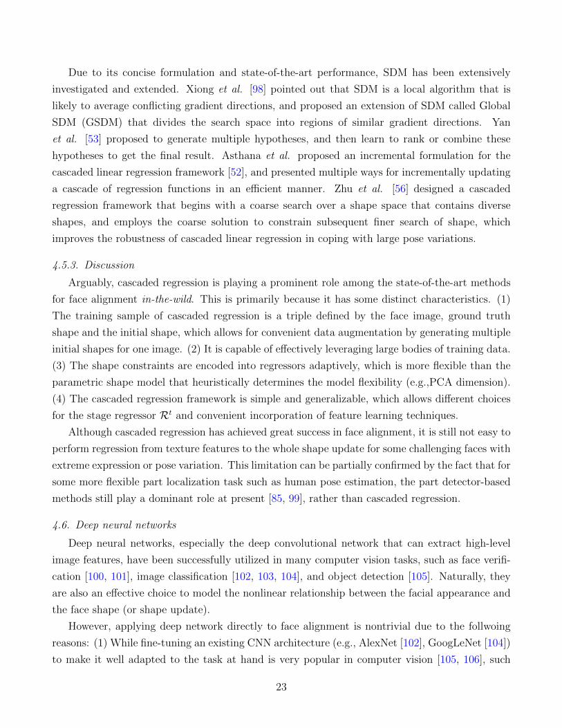
Due to its concise formulation and state-of-the-art performance, SDM has been extensively
investigated and extended. Xiong et al. [98] pointed out that SDM is a local algorithm that is
likely to average conflicting gradient directions, and proposed an extension of SDM called Global
SDM (GSDM) that divides the search space into regions of similar gradient directions. Yan
et al. [53] proposed to generate multiple hypotheses, and then learn to rank or combine these
hypotheses to get the final result. Asthana et al. proposed an incremental formulation for the
cascaded linear regression framework [52], and presented multiple ways for incrementally updating
a cascade of regression functions in an efficient manner. Zhu et al. [56] designed a cascaded
regression framework that begins with a coarse search over a shape space that contains diverse
shapes, and employs the coarse solution to constrain subsequent finer search of shape, which
improves the robustness of cascaded linear regression in coping with large pose variations.
4.5.3. Discussion
Arguably, cascaded regression is playing a prominent role among the state-of-the-art methods
for face alignment in-the-wild. This is primarily because it has some distinct characteristics. (1)
The training sample of cascaded regression is a triple defined by the face image, ground truth
shape and the initial shape, which allows for convenient data augmentation by generating multiple
initial shapes for one image. (2) It is capable of effectively leveraging large bodies of training data.
(3) The shape constraints are encoded into regressors adaptively, which is more flexible than the
parametric shape model that heuristically determines the model flexibility (e.g.,PCA dimension).
(4) The cascaded regression framework is simple and generalizable, which allows different choices
for the stage regressor Rt and convenient incorporation of feature learning techniques.
Although cascaded regression has achieved great success in face alignment, it is still not easy to
perform regression from texture features to the whole shape update for some challenging faces with
extreme expression or pose variation. This limitation can be partially confirmed by the fact that for
some more flexible part localization task such as human pose estimation, the part detector-based
methods still play a dominant role at present [85, 99], rather than cascaded regression.
4.6. Deep neural networks
Deep neural networks, especially the deep convolutional network that can extract high-level
image features, have been successfully utilized in many computer vision tasks, such as face verifi-
cation [100, 101], image classification [102, 103, 104], and object detection [105]. Naturally, they
are also an effective choice to model the nonlinear relationship between the facial appearance and
the face shape (or shape update).
However, applying deep network directly to face alignment is nontrivial due to the follwoing
reasons: (1) While fine-tuning an existing CNN architecture (e.g., AlexNet [102], GoogLeNet [104])
to make it well adapted to the task at hand is very popular in computer vision [105, 106], such
23

a strategy can hardly be applied for face alignment because the off-the-shelf large networks are
typically trained for image classification while face alignment is a structural prediction problem.
(2) Constructing a deep network-based system from scratch for face alignment should take into
account the issue of over-fitting, and hence the network structures at each stage need to be carefully
designed according to the task of this stage and the complexity involved.
Figure 2: Three-level cascaded convolutional networks. The input is the face region returned by a face detector. The threenetworks at level 1 are denoted as F1, EN1, and NM1. Networks at level 2 are denoted as LE21, LE22, RE21, RE22, N21,N22, LM21, LM22, RM21, and RM22. Both LE21 and LE22 predict the left eye center, and so forth. Networks at level 3are denoted as LE31, LE32, RE31, RE32, N31, N32, LM31, LM32, RM31, and RM32. Green square is the face boundingbox given by the face detector. Yellow shaded areas are the input regions of networks. Red dots are the final predictions ateach level. Dots in other colors are predictions given by individual networks.
Figure 3: The structure of deep convolutional network F1.Sizes of input, convolution, and max pooling layers are il-lustrated by cuboids whose length, width, and height denotethe number of maps, and the size of each map. Local recep-tive fields of neurons in different layers are illustrated bysmall squares in the cuboids.
multaneously predicts multiple facial points. For each facialpoint, the predictions of multiple networks are averaged toreduce the variance. Figure 3 illustrates the deep structureof F1, which contains four convolutional layers followed bymax pooling, and two fully connected layers. EN1 and N-M1 take the same deep structure, but with different sizesat each layer since the sizes of their input regions are dif-ferent. Networks at the second and third levels take localpatches centered at the predicted positions of facial pointsfrom previous levels as input and are only allowed to makesmall changes to previous predictions. The sizes of patchesand search ranges keep reducing along the cascade. Pre-dictions at the last two levels are strictly restricted becauselocal appearance is sometimes ambiguous and unreliable.The predicted position of each point at the last two levelsis given by the average of the two networks with differentpatch sizes. While networks at the first level aim to estimatekeypoint positions robustly with few large errors, networksat the last two levels are designed to achieve high accura-cy. All the networks at the last two levels share a common
shallower structure since their tasks are low-level.
3.1. Network structure selection
We analyze three important factors on the choice of net-work structures. The discussions are limited to networks atthe first level, which are the hardest to train. First, convo-lutional networks at the first level should be deep. Predict-ing keypoints from large input regions is a high-level task.Deeper structures help to form high-level features, whichare global while features extracted by neurons at lower lay-ers are local due to local receptive fields. By combiningspatially nearby features extracted at lower layers, neuron-s at higher layers can extract features from larger regions.Moreover, high-level features are highly non-linear. Addingadditional layers increases the non-linearity from input tooutput, and makes it possible to represent the relationshipbetween input and output.
Second, for neurons in the convolutional layers, abso-lute value rectification after the hyperbolic tangent activa-tion function (see details in Section 4) can effectively im-prove the performance. This modification over traditionalconvolutional networks was proposed in [14], where im-provement on Caltech-101 was observed. Our empirical s-tudy shows that it is also effective in our application.
Third, locally sharing weights of neurons on the samemap improves the performance. Traditional convolution-al networks share weights of all the neurons on the samemap based on two considerations. First, it assumes thatthe same features may appear everywhere in an image. Sofilters useful in one place should also be useful in others.Second, weight sharing helps to prevent gradient diffusionwhen back-propagating through many layers, since gradi-ents of shared weights are aggregated, which makes super-vised learning on deep structures easier. However, globally
347634763478
Figure 6: One of the first-level convolutional neural network structures used in [57] to predict five major facialpoints. Sizes of input, convolution, and max pooling layers are illustrated by cuboids whose length, width, andheight denote the number of maps, and the size of each map. Local receptive fields of neurons in different layersare illustrated by small squares in the cuboids.
Focusing on above issues, Sun et al. [57] were pioneers in this area with their work called
Deep Convolutional Network Cascade. They handled the face alignment task with three-level
carefully designed convolutional networks, and fuse the outputs of multiple networks at each level
for robust prediction (Fig. 6 illustrates one of the first-level CNN structures). The first level
network takes the whole face image as input to predict the initial estimates of the holistic face
shape, during which the shape constraints are implicitly encoded. Then, the following two level
networks refine the position of each point to achieve higher accuracy. Several network structures
critical for face alignment are investigated in [57], providing some important principles on the
choice of convolutional network structures. For example, convolutional networks at the first level
should be deeper than the following networks, since predicting facial points from large input regions
is a high-level task.
Ever since the work of [58], deep CNNs have been widely exploited for face alignment. Similar
to [58], Zhou et al. [107] designed a four-level convolutional network cascade to tackle the face
alignment problem in a coarse-to-fine manner, where each network level is trained to locally refine
a subset of facial points generated by previous network levels. Zhang et al. [58] extended the work
of [57] by jointly learning auxiliary attributes along with face alignment. Their work confirms that
some heterogeneous but subtly correlated tasks, e.g., head pose estimation and facial attribute
inference can aid the face alignment task through multi-task learning. Lai et al. [59] proposed an
end-to-end CNN architecture to learn highly discriminative shape-indexed features, by encoding the
image into high-level feature maps in the same size of the image, and then extracting deep features
from these high level descriptors through a novel “Shape-Indexed Pooling” method. Despite of
the great popularity and success, as mentioned before, we should take into account the tradeoff
between the model complexity and training data size, since some deep models have been reported
24

to be pre-trained with enormous quantity of external data sources [57, 58].
4.7. Summary and discussion
We have reviewed discriminative methods for face alignment in six groups, i.e., CLMs, con-
strained local regression, DPMs, ensemble regression-voting, cascaded regression and deep neural
networks. Among them, CLMs, constrained local regression and DPMs follow the “divide and
conquer” principle to simplify the face alignment task by constructing individual local appearance
model for each facial point. However, due to their small patch support and large appearance varia-
tion in training, these local appearance models are typically plagued by the problem of ambiguity.
Furthermore, since further inference (or global shape optimization) is based on the detection re-
sponses of these local appearance models, the problem of ambiguity may create the most serious
performance bottleneck for face alignment in-the-wild.
To break this bottleneck, another main stream in face alignment is to jointly estimate the whole
face shape from image, implicitly exploiting the spatial constraints among facial points. In this line,
we have first reviewed the ensemble regression-voting and cascaded regression methods, which learn
a vectorial regression function to infer the whole face shape in an ensemble or cascaded manner.
In particular, cascaded regression has emerged as one of the most popular and state-of-the-art
methods, due to its speed, accuracy and robustness. Then, we briefly reviewed the deep learning-
based approach for face alignment, which have the advantage of learning highly discriminative
task-specific features, but should take into account the issue of over-fitting.
It is worth noting that some methods involve techniques motivated by different principles,
which clearly overlap our category boundaries. For example, we classify the regression voting-
based shape model matching method [30] as CLM, since they fit a parametric shape model to a
new image based on the response map for each facial point. However, since the response maps in
[30] are generated by random forest regression-voting, it can also be considered as an ensemble
regression-voting method. Furthermore, some deep learning-based methods can also be classified
as cascaded regression due to their cascaded structure [60, 59].
5. Towards the development of a robust face alignment system
Face alignment in-the-wild is very challenging due to many kinds of undesirable appearance
variations, and hence it is often the case that no single modality is enough. In this section, we
will focus on the practical aspects of constructing a robust face alignment system, which is mostly
ignored in previous studies. Specifically, we first present a global system architecture for face
alignment, and then have a close look at possible strategies to improve the robustness of face
alignment under this architecture.
25

Normalization Acquisition
Face Detection
Input Image
Face Image
Scaling +
Lighting +
Enlarging
Normalized Face
Face Preprocessing
Mean Shape /
Randomly Sampled Shape
/ Multiple Randomly
Sampled Shapes /
Anchor Point-based Initialization
/ Estimation-based
Initialization
Shape Initialization Feature Extraction
Eye Center Coordinate
+ Eye Corner Coordinate
+ Nose Tip
Coordinate +
Mouth Corner Coordinate
+ Chin Coordinate
+ …
Output
Hand-designed Feature:
SIFT HOG
Learned Shallow Feature: Pixel Difference
LBF
Learned Deep Representation:
CNN
Shape Prediction
Generative Methods:
AAM Fitting/ Pictorial Structure
Discriminative Methods: Random Forests/
Cascaded Regression/
Structural SVM/ Hough Voting
Figure 7: A global system architecture for face alignment.
5.1. The global system architecture for face alignment
Inspired by [108, 109], we give a global system architecture for face alignment, where a com-
plicated system is divided into several substages. As shown in Fig. 7, the architecture can be
roughly divided into three parts: face preprocessing, shape initialization, and the iterative process
of feature extraction and shape prediction. We note that this architecture is only to illustrate
a general pipeline for face alignment, while in practical not all components are mandatory. For
example, the consensus of exemplar method [11] do not involve the shape initialization step.
While the feature extraction and shape prediction process have drawn a great deal of attention
in literature, the face preprocessing and shape initialization steps are often ignored. Meanwhile,
problems such as training data augmentation, and the accuracy and efficiency tradeoff are also
essential for any practical face alignment system. In the following, we will have a closer look at
these issues.
5.2. Training data augmentation
Due to the difficulty and cost of manual annotation, the number of training samples we actually
have is often much smaller than that we supposedly have. In such a case, artificial data augmenta-
tion, which is usually done by label-preserving transforms, is the easiest and most common method
to reduce over-fitting.
In general, there are four distinct forms of data augmentation to enlarge the training set: (1)
generating image rotations from a small interval (e.g., [-15 degrees, +15 degrees] used in [83]); (2)
synthesizing images by left-right flip to double the training set; (3) disturbing the bounding boxes
by randomly scaling and translating the bounding box for each image, which also increases the
robustness of face alignment algorithms to the bounding boxes; (4) sampling multiple initialization
for each training image, which is typically used by cascaded regression methods.
26

5.3. Face preprocessing
For the task of face alignment, it is useful to remove the scaling variations of the detected faces,
and enlarge the face region to ensure that all predefined facial points are enclosed.
5.3.1. Handling scaling variations
Typically, for a face analysis system, the training and test faces are required to be roughly
the same scale, by rescaling the bounding box produced by the face detector. We note that
to help preserve more detailed texture information, the size of the normalized bounding box for
high-resolution face databases is typically chosen to be larger than that for low-resolution face
databases. For example, Belhumeur et al. [83] rescale the high-resolution images from the LFPW
database so that the faces have an inter-ocular distance of roughly 55 pixels, while Dantone et al.
[12] choose to rescale the bounding box of the low-resolution faces from the LFW database [96] to
100×100, which is slightly smaller than the size chosen by Belhumeur et al. [83].
5.3.2. Enlarging face areas
The output of a face detector is a rough face region that might miss some facial points (e.g.,
the chin). This has little impact on cascaded regression, for which the bounding box only serves
to rescale the face and compute the initial shape. However, for those methods based on exhaustive
search or feature voting, it is necessary to enlarge the face bounding box to enclose all the facial
points, or define the sampling region of image patches to cast votes. For this, Dantone et al. [12]
suggest to enlarge the face bounding box by 30%, and we believe that this strategy may satisfy
the requirements of all face alignment algorithms.
5.4. Shape initialization
Most face alignment methods start from a rough initialization, and then refine the shape
iteratively until convergence. The initialization step typically has great influence on the final
result, and an initial shape far from the ground truth might lead to very bad alignment results.
The most common choice is to use the mean shape for initialization [52, 50, 54]. However,
sometimes, the mean shape is likely to be far from the target shape, and leads to bad result. As an
alternative, Cao et al. [48] propose to run the algorithm several times using different initialisations
randomly sampled from the training shapes, and take the median result as the final estimation to
improve robustness. Burgos-Artizzu et al. [49] proposed a smart restart method to further improve
the multiple initialization strategy in [48] by checking the variance between the predictions using
different initializations.
Recently, some authors proposed to estimate an initial shape that is tailored to the input face.
Zhang et al. [58] showed that the five major facial points localized by their deep model can serve as
anchor points to apply similarity transform to randomly sampled training shapes. Through this,
27

very accurate initial shapes can be generated for other algorithms (e.g., [49]) and lead to promising
performance improvement. Zhang et al. [60] and Sun et al. [57] proposed to directly estimate a
rough initial shape from the global image, which in general produces good initial shape that aids
following alignment.
5.5. Accuracy and efficiency tradeoffs
Face alignment in real time is crucial to many practical applications. The efficiency mainly
depends on the feature extraction and shape prediction steps. In general, strong hand-designed
feature (e.g., SIFT [78]) captures detailed texture information that may aid detection, but have
higher computational cost compared to simpler features (e.g., BRIEF [110]). Zhu et al. [56]
identified this phenomenon under the cascaded regression framework, and proposed to exploit
different types of features at different stages to achieve a good trade-off between accuracy and
efficiency, i.e., employ less accurate but computationally efficient BRIEF feature at the early stages,
and use more accurate but relatively slow SIFT feature at later stages. Besides this hybrid strategy,
a better choice is to learn highly efficient and discriminative features [48, 54, 50]. In particular,
Ren et al. [54] propose to learn a set of highly discriminative local binary features for each facial
point independently. Because extracting and regressing local binary features is computationally
very cheap, [54] achieves over 3,000 FPS while obtaining accurate alignment result.
In term of shape prediction, the regression-based methods in general are very efficient, while the
exhaustive search based methods typically suffer from high computational cost [11, 33]. Dibeklioglu
et al. [111] propose to mitigate this issue through a coarse-to-fine search strategy. In [111], a three-
level image pyramid from the cropped high-resolution face images is designed to reduce the search
region, where the coarse-level images have lower resolution but much smaller size.
6. System Evaluation
In this section, we first review the major wild face databases and evaluation metric in the
literature, then summarize and discuss some of reported performance of current state-of-the-art,
on the several popular wild face databases using the same evaluation metric for reference.
6.1. Databases and metric
6.1.1. Databases
There have been many face databases developed for face alignment, with the ground truth facial
points labelled manually by employing workers or through the tools such as Amazon mechanical
turk (MTurk). Among them, some databases are collected under controlled laboratory conditions
with normal lighting, neutral expression and high image quality, including the Extended M2VTS
database (XM2VTS) [115], BioID face database [116], PUT [117], Multi-Pie [118], etc.
28

Table 4: A list of sources of wild databases for face alignment.Databases Year #Images #Training #Test #Point Links
LFW [96] 2007 13,233 1,100 300 10 http://www.dantone.me/datasets/facial-features-lfw/
LFPW [11] 2011 1,432a - - 35b http://homes.cs.washington.edu/~neeraj/databases/lfpw/
AFLW [112] 2011 25,993 - - 21 http://lrs.icg.tugraz.at/research/aflw
AFW [41] 2012 205 - - 6 http://www.ics.uci.edu/~xzhu/face/
HELEN [84] 2012 2,330 2,000 300 194 http://www.ifp.illinois.edu/~vuongle2/helen/
300-W [113] 2013 3,837 3,148 689 68 http://ibug.doc.ic.ac.uk/resources/300-W/
COFW [49] 2013 1,007 - - 29 http://www.vision.caltech.edu/xpburgos/ICCV13/
MTFL [58] 2014 12,995 - - 5 http://mmlab.ie.cuhk.edu.hk/projects/TCDCN.html
MAFL [114] 2016 20,000 - - 5 http://mmlab.ie.cuhk.edu.hk/projects/TCDCN.htmla LFPW is shared by web URLs, but some URLs are no longer valid.b Each face image in LFPW is annotated with 35 points, but only 29 points defined in [11] are used for the face alignment.
(a) LFW (b) LFPW (c) AFLW (d) AFW
(e) HELEN (f) 300-W (g) COFW (h) MTFL
Figure 8: Illustration of the example face images from eight wide face databases with original annotation.
However, the goal of this paper is to investigate the problem of face alignment in-the-wild,
so we are more concerned with the uncontrolled databases that exhibit large facial variations
due to pose, expressions, lighting, occlusion and image quality. These uncontrolled databases are
typically collected from social network such as google.com, flickr.com, facebook.com, which are
more realistic and challenging for face alignment. In Tab. 4, we list the basic information of 9
wild face databases, including LFW [96], LFPW [11], AFLW [112], AFW [41], HELEN [84], 300-W
[113], COFW [49], MTFL [58], and MAFL [114], and also provide links to download them. The
example face images from these databases with original annotation are illustrated in Fig. 8. It
is worth noting that the LFPW, AFW and HELEN databases are re-annotated by Sagonas et al.
[113] with 68 points.
6.1.2. Evaluation metric
There have been several evaluation metrics for the alignment accuracy in the literature. For
example, many authors reported the inter-pupil distance normalized facial point error averaged
over all facial points and images for each database [49, 54, 50, 56, 51]. Specifically, the inter-ocular
29

distance normalized error for facial point i is defined as:
ei =||xi − x∗i ||2dIOD
, (10)
where xi is the automatically localized facial point location, x∗i is the manually annotated loca-
tion, and dIOD is the inter-ocular distance. The normalization term dIOD in this formulation can
eliminate unreasonable measurement variations caused by variations of face scales.
The cumulative errors distribution (CED) curve is also often chosen to illustrate the compar-
ative performance, showing the proportion of the test images or facial points with the increase
of the normalized error [29, 11, 26, 27, 56]. Some other evaluation metric can also been found in
literature, such as the facial point error normalized by face size [43], the percentage of the test
images or facial points less than given relative error level [111, 43], and the percentage of accuracy
improvement over other algorithm [48].
Besides the accuracy, the efficiency is another important performance indicator of face align-
ment algorithms, which is typically measured by frames per second (FPS).
6.2. Evaluation and discussion
Table 5: A list of published software of face alignment.Methods Year #Points LinksBoosted Regression with Markov Networks (BoRMaN) [38] 2010 22 http://ibug.doc.ic.ac.uk/resources/facial-point-detector-2010/
Constrained Local Model (CLM) [29] 2011 66 https://github.com/kylemcdonald/FaceTracker
Tree Structured Part Model (TSPM) [41] 2012 68 http://www.ics.uci.edu/~xzhu/face/
Conditional Random Forests (CRF) [12] 2012 10 http://www.dantone.me/projects-2/facial-feature-detection/
Structured Output SVM [42] 2012 7 http://cmp.felk.cvut.cz/~uricamic/flandmark/
Cascaded CNN [57] 2013 5 http://mmlab.ie.cuhk.edu.hk/archive/CNN_FacePoint.htm
Discriminative Response Map Fitting (DRMF) [31] 2013 66 https://sites.google.com/site/akshayasthana/clm-wild-code?
Supervised Descent Method (SDM) [52] 2013 49 www.humansensing.cs.cmu.edu/intraface
Robust Cascaded Pose Regression (RCPR) [49] 2013 29 http://www.vision.caltech.edu/xpburgos/ICCV13/
Optimized Part Mixtures (OPM) [43] 2013 68 http://www.research.rutgers.edu/~xiangyu/face_align/face_
align_iccv_1.1.zip
Continuous Conditional Neural Fields (CCNF) [119] 2014 68 https://github.com/TadasBaltrusaitis/CCNF
Coarse-to-fine Shape Searching (CFSS) [56] 2015 68 mmlab.ie.cuhk.edu.hk/projects/CFSS.html
Project-Out Cascaded Regression (PO-CR) [27] 2015 68 http://www.cs.nott.ac.uk/~yzt/
Active Pictorial Structures (APS) [28] 2015 68 https://github.com/menpo/menpo
Tasks-Constrained Deep Convolutional Network (TCDCN)[114]
2016 68 http://mmlab.ie.cuhk.edu.hk/projects/TCDCN.html
We choose four common wild databases, i.e., LFW, LFPW, HELEN, 300-W and IBUG (chal-
lenging subset of 300-W) databases, to show comparative performance statistics of the state of the
art. Table 5 lists some softwares published online, and Table 6 summarizes the reported perfor-
mance on above databases. Fig. 10 shows some challenging images from IBUG aligned by eight
state-of-the-art methods respectively.
For performance evaluation, we are mainly concerned with two key performance indicators, i.e.,
accuracy and efficiency. The former is measured by the normalized facial point error (cf. Eq. 10)
averaged over all facial points and images for each database, while the later is measured by frames
per second (FPS).
30
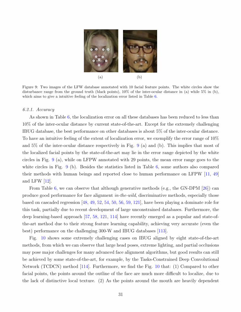
(a) (b)
Figure 9: Two images of the LFW database annotated with 10 facial feature points. The white circles show thedisturbance range from the ground truth (black points), 10% of the inter-ocular distance in (a) while 5% in (b),which aims to give a intuitive feeling of the localization error listed in Table 6.
6.2.1. Accuracy
As shown in Table 6, the localization error on all these databases has been reduced to less than
10% of the inter-ocular distance by current state-of-the-art. Except for the extremely challenging
IBUG database, the best performance on other databases is about 5% of the inter-ocular distance.
To have an intuitive feeling of the extent of localization error, we exemplify the error range of 10%
and 5% of the inter-ocular distance respectively in Fig. 9 (a) and (b). This implies that most of
the localized facial points by the state-of-the-art may lie in the error range depicted by the white
circles in Fig. 9 (a), while on LFPW annotated with 29 points, the mean error range goes to the
white circles in Fig. 9 (b). Besides the statistics listed in Table 6, some authors also compared
their methods with human beings and reported close to human performance on LFPW [11, 49]
and LFW [12].
From Table 6, we can observe that although generative methods (e.g., the GN-DPM [26]) can
produce good performance for face alignment in-the-wild, discriminative methods, especially those
based on cascaded regression [48, 49, 52, 54, 50, 56, 59, 121], have been playing a dominate role for
this task, partially due to recent development of large unconstrained databases. Furthermore, the
deep learning-based approach [57, 58, 121, 114] have recently emerged as a popular and state-of-
the-art method due to their strong feature learning capability, achieving very accurate (even the
best) performance on the challenging 300-W and IBUG databases [113].
Fig. 10 shows some extremely challenging cases on IBUG aligned by eight state-of-the-art
methods, from which we can observe that large head poses, extreme lighting, and partial occlusions
may pose major challenges for many advanced face alignment algorithms, but good results can still
be achieved by some state-of-the-art, for example, by the Tasks-Constrained Deep Convolutional
Network (TCDCN) method [114]. Furthermore, we find the Fig. 10 that: (1) Compared to other
facial points, the points around the outline of the face are much more difficult to localize, due to
the lack of distinctive local texture. (2) As the points around the mouth are heavily dependent
31

Figure 10: Example results on IBUG database [4] by eight state-of-the-art methods. These images are extremelydifficult due to the mixing of large head poses, extreme lighting, and partial occlusions. From top to bottom,results are produced by the Project-Out Cascaded Regression (PO-CR) method [27], Consensus of Exemplar (CoE)method [83], Robust Discriminative Hough Voting (RDHV) method [34], Local Binary Feature (LBF) method[54], Supervised Descent Method (SDM) [52], Explicit Shape Regression (ESR) method [48], Coarse-to-Fine ShapeSearching (CFSS) method [56], Tasks-Constrained Deep Convolutional Network (TCDCN) method [114]. Amongthese methods, we implement the Consensus of Exemplar (CoE) [83] and Robust Discriminative Hough Voting(RDHV) [34] methods and test them on these images, while other results are obtained from the published papers.
on facial expressions, they are more difficult to localize than those points insensitive to facial
32

Table 6: Lists of face alignment performance evaluated on various wild face databases.Databases Challenges #Test #Points Methods Error (%) FPS
LFW[96]
Low resolution, largevariations inilluminations,expressions and poses
13,233a 10
Conditional Random Forests (CRF) [12] 7.00 10 (c++)Explicit Shape Regression (ESR) [48] 5.90 11 (Matlab)Robust Cascaded Pose Regression (RCPR) [49] 5.30 15 (Matlab)
55b Consensus of Exemplar (CoE) [83] 5.18 -
LFPW[11]
Large variations inilluminations,expressions, poses andocclusion
224∼300c
21
Consensus of Exemplar (CoE) [11] 3.99 ≈ 1 (C++)Explicit Shape Regression (ESR) [48] 3.47 220 (C++)Robust Cascaded Pose Regression (RCPR) [49] 3.50 12 (Matlab)Supervised Descent Method (SDM) [52] 3.49 160 (C++)Exemplar-based Graph Matching (EGM) [33] 3.98 < 1Local Binary Feature (LBF) [54] 3.35 460 (C++)Fast Local Binary Feature (LBF fast) [54] 3.35 4600 (C++)
68d
Tree Structured Part Model (TSPM) [41] 8.29 0.04 (Matlab)Discriminative Response Map Fitting (DRMF) [31] 6.57 1 (Matlab)Robust Cascaded Pose Regression (RCPR) [49] 6.56 12 (Matlab)Supervised Descent Method (SDM) [52] 5.67 70 (C++)Gauss-Newton Deformable Part Model (GN-DPM) [26] 5.92 70Coarse-to-fine Auto-encoder Networks (CFAN) [60] 5.44 20Coarse-to-fine Shape Searching (CFSS) [56] 4.87 -CFSS Practical [56] 4.90 -Deep Cascaded Regression (DCR) [59] 4.57 -
HELEN[84]
Computation burdendue to the denseannotation, largevariations inexpressions, poses andocclusion
330
194
Stacked Active Shape Model (STASM) [120] 11.10 -Component-based ASM (ComASM) [84] 9.10 -Explicit Shape Regression (ESR) [48] 5.70 70 (C++)Robust Cascaded Pose Regression (RCPR) [49] 6.50 6 (Matlab)Supervised Descent Method (SDM) [52] 5.85 21 (C++)Ensemble of Regression Trees (ERT) [50] 4.9 1000Local Binary Feature (LBF) [54] 5.41 200 (C++)Fast Local Binary Feature (LBF fast) [54] 5.80 1500 (C++)Coarse-to-Fine Shape Searching (CFSS) [56] 4.74 -CFSS Practical [56] 4.84 -cascade Gaussian Process Regression Trees (cGPRT)[51]
4.63 -
68d
Tree Structured Part Model (TSPM) [41] 8.16 0.04 (Matlab)Discriminative Response Map Fitting (DRMF) [31] 6.70 1 (Matlab)Robust Cascaded Pose Regression (RCPR) [49] 5.93 12 (Matlab)Supervised Descent Method (SDM) [52] 5.67 70 (C++)Gauss-Newton Deformable Part Model (GN-DPM) [26] 5.69 70Coarse-to-fine Auto-encoder Networks (CFAN) [60] 5.53 20Coarse-to-Fine Shape Searching (CFSS) [56] 4.63 -CFSS Practical [56] 4.72 -Deep Cascaded Regression [59] 4.25 -
300-W[113]
Large variations inilluminations,expressions, poses andocclusion
689 68
Tree Structured Part Model (TSPM) [41] 12.20 0.04 (Matlab)Discriminative Response Map Fitting (DRMF) [31] 9.10 1 (Matlab)Explicit Shape Regression (ESR) [48] 5.28 120 (C++)Robust Cascaded Pose Regression (RCPR) [49] 8.35 -Supervised Descent Method (SDM) [52] 7.50 70 (C++)Ensemble of Regression Trees (ERT) [50] 6.4 1000Local Binary Feature (LBF) [54] 6.32 320 (C++)Fast Local Binary Feature (LBF fast) [54] 7.37 3100 (C++)Coarse-to-Fine Shape Searching (CFSS) [56] 5.76 25CFSS Practical [56] 5.99 25cascade Gaussian Process Regression Trees (cGPRT)[51]
5.71 93
fast cGPRT [51] 6.32 871Tasks-Constrained Deep Convolutional Network(TCDCN) [114]
5.54 59
Deep Cascaded Regression (DCR) [59] 5.02 -Megvii-Face++ [121] 4.54 -
IBUG[113]
Extremely largevariations inilluminations,expressions, poses andocclusion
135 68
Tree Structured Part Model (TSPM) [41] 18.33 0.04 (Matlab)Discriminative Response Map Fitting (DRMF) [31] 19.79 1 (Matlab)Explicit Shape Regression (ESR) [48] 17.00 120 (C++)Robust Cascaded Pose Regression (RCPR) [49] 17.26 -Supervised Descent Method (SDM) [52] 15.40 70 (C++)Local Binary Feature (LBF) [54] 11.98 320 (C++)Fast Local Binary Feature (LBF fast) [54] 15.50 3100 (C++)Robust Discriminative Hough Voting (RDHV) [34] 11.32 < 1 (Matlab)Coarse-to-Fine Shape Searching (CFSS) [56] 9.98 25CFSS Practical [56] 10.92 25Tasks-Constrained Deep Convolutional Network(TCDCN) [114]
8.60 59
Deep Cascaded Regression (DCR) [59] 8.42 -Megvii-Face++ [121] 7.46 -
a For LFW, the reported performance of [12, 48, 49] follows the the evaluation procedure proposed in [12], consisting of a ten-fold cross validation using eachtime 1,500 training images and the rest for testing. In [83], the model is trained on Columbia’s PubFig [5], and tested on all 13,233 images of LFW.
b Although used by [83], the 55 point annotation of LFW is not shared.c LFPW is shared by web URLs, but some URLs are no longer valid. So both the training and test images downloaded by other authors are less than the
original version (1,100 training images and 300 test images).d LFPW and HELEN are originally annotated with 29 and 194 points respectively, while later Sagonas et al. [113] re-annotate them with 68 points. Some
authors reported their performance on the 68 points version of these databases.
33

expressions, such as the points along the eyebrows, outer corners of the eyes, and the nose tips.
Finally, we have to highlight that the accuracy statistics listed in Table 6 may not fully charac-
terize the behavior of these algorithms, since several factors can complicate the assessment. First,
even for the same algorithm, different experimental details and programming skills may results in
different performance. Secondly, while the number and variety of training examples have a direct
effect on the final performance, the training data of some released software is not clear. Thirdly,
as pointed by [15], the performance of many algorithms is sensitive to the face detection variation,
but different systems may employ different face detectors. For example, SDM [52] employs the
Viola Jones detector [122], while GN-DPM [26] uses the in-house face detector of the IBUG group.
6.2.2. Efficiency
Besides accuracy, efficiency is another key performance indicator of face alignment algorithms.
In the last column of Table 6, we report the efficiency of some algorithms, and highlight the
implementation types of them (Matlab or C++). In general, the running time listed here is
consistent with the algorithm’s complexity. For example, algorithms that involves an exhaustive
search of local detectors typically have a high time cost [11, 41, 33], while the cascaded regression
methods are extremely fast since both the shape-index feature and the stage regression are very
efficient to compute [48, 52, 49]. It is worth noting that impressive speed (more than 1,000 FPS for
194 points on HELEN) has been achieved by the Local Binary Feature (LBF) [54] and Ensemble
of Regression Trees (ERT) [50], using learning-based features.
7. Conclusion and prospect
Face alignment is an important and essential intermediary step for many face analysis applica-
tions. Such a task is extremely challenging in unconstrained environments due to the complexity
of facial appearance variations. However, extensive studies on this problem have resulted in a great
amount of achievements, especially during the last few years.
In this paper, we have focused on the overall difficulties and challenges in unconstrained envi-
ronments, and provide a comprehensive and critical survey of the current state of the art in dealing
with these challenges. Furthermore, we hope that the practical aspects of face alignment we orga-
nized can provide further impetus for high-performance, real-time, real-life face alignment systems.
Finally, it is worth mentioning that some closely related problems are deliberately ignored in this
paper, such as facial feature tracking in videos [123, 124] and 3D face alignment [125], which are
also very important in practice.
Despite of many efforts devoted to face alignment during the last two decades, we have to admit
that this problem is far from being solved, and several general promising research directions could
be suggested.
34

• Challenging databases collection: Besides new methodologies, another notable development
in the field of face alignment has been the collection and annotation of large facial datasets
captured in-the-wild (cf., Table 4). But even so, we argue that the collection of challenging
databases is still important and has the potential to boost the performance of existing meth-
ods. This argument can be partially supported by the fact that: the performance of most
algorithms on IBUG is inferior to that on other databases such as LFPW and HELEN, as
the training set of these algorithms is typically less challenging compared to IBUG.
• Feature learning: One of the holy grails of machine learning is to automate more and more
of the feature engineering process [126], i.e., to learn task-specific features in a data-driven
manner. In the field of face alignment, many approaches that employ feature learning tech-
niques, including both shallow feature learning [48, 49, 54] and deep learning [57, 121] meth-
ods, have achieved state-of-the-art performances. We believe that, with the assistance of
abundant manually labeled images, automatic feature learning techniques can be a powerful
weapon for triumphing over various challenges of face alignment in the wild, and deserve the
efforts and smarts of researchers.
• Multi-task learning: Multi-task learning aims to improve the generalization performance of
multiple related tasks by learning them jointly, which has proven effective in many computer
vision problems [127, 128]. For face alignment in-the-wild, on the one hand, many factors
such as pose, expression and occlusion may pose great challenges; while on the other hand,
these factors can be considered jointly with face alignment to expect an improvement of
robustness. This has been confirmed by the work of [58], which proposes to exploit the
power of multi-task learning under the deep convolutional network architecture, leading to
a better performance compared to single task-based deep model. Although some attempts
have been proposed, we believe that multi-task learning remains a meaningful and promising
direction for face alignment in future.
We believe that face alignment in-the-wild is a very exciting line of research due to its inherent
complexity and wide practical applications, and will draw increasing attention from computer
vision, pattern recognition and machine learning.
Acknowledgment
This work is partially supported by National Science Foundation of China (61373060), Qing Lan
Project, and the Funding of Jiangsu Innovation Program for Graduate Education (KYLX 0289).
35

References
[1] S. Zafeiriou, C. Zhang, Z. Zhang, A survey on face detection in thewild: past, present and future, Computer Vision and Image Under-standing 138 (2015) 1–24.
[2] W. Zhao, R. Chellappa, P. J. Phillips, A. Rosenfeld, Face recognition:A literature survey, Acm Computing Surveys (CSUR) 35 (4) (2003)399–458.
[3] P. Campadelli, R. Lanzarotti, C. Savazzi, A feature-based face recog-nition system, in: Image Analysis and Processing, 2003. Proceedings.12th International Conference on, IEEE, 2003, pp. 68–73.
[4] C. Sagonas, G. Tzimiropoulos, S. Zafeiriou, M. Pantic, 300 faces in-the-wild challenge: The first facial landmark localization challenge,in: Computer Vision Workshops (ICCVW), 2013 IEEE InternationalConference on, IEEE, 2013, pp. 397–403.
[5] N. Kumar, A. C. Berg, P. N. Belhumeur, S. K. Nayar, Attribute andsimile classifiers for face verification, in: Computer Vision, 2009 IEEE12th International Conference on, IEEE, 2009, pp. 365–372.
[6] O. Rudovic, I. Patras, M. Pantic, Coupled gaussian process regressionfor pose-invariant facial expression recognition, in: Computer Vision–ECCV 2010, Springer, 2010, pp. 350–363.
[7] M. F. Valstar, M. Pantic, Fully automatic recognition of the tempo-ral phases of facial actions, Systems, Man, and Cybernetics, Part B:Cybernetics, IEEE Transactions on 42 (1) (2012) 28–43.
[8] T. Senechal, V. Rapp, H. Salam, R. Seguier, K. Bailly, L. Prevost,Combining aam coefficients with lgbp histograms in the multi-kernelsvm framework to detect facial action units, in: Automatic Face &Gesture Recognition and Workshops (FG 2011), 2011 IEEE Interna-tional Conference on, IEEE, 2011, pp. 860–865.
[9] J. N. Bailenson, E. D. Pontikakis, I. B. Mauss, J. J. Gross, M. E.Jabon, C. A. Hutcherson, C. Nass, O. John, Real-time classifica-tion of evoked emotions using facial feature tracking and physiologi-cal responses, International journal of human-computer studies 66 (5)(2008) 303–317.
[10] H. Li, H. Ding, D. Huang, Y. Wang, X. Zhao, J.-M. Morvan, L. Chen,An efficient multimodal 2d+ 3d feature-based approach to automaticfacial expression recognition, Computer Vision and Image Understand-ing 140 (2015) 83–92.
[11] P. N. Belhumeur, D. W. Jacobs, D. Kriegman, N. Kumar, Localizingparts of faces using a consensus of exemplars, in: Computer Visionand Pattern Recognition (CVPR), 2011 IEEE Conference on, IEEE,2011, pp. 545–552.
[12] M. Dantone, J. Gall, G. Fanelli, L. Van Gool, Real-time facial featuredetection using conditional regression forests, in: Computer Visionand Pattern Recognition (CVPR), 2012 IEEE Conference on, IEEE,2012, pp. 2578–2585.
[13] O. Celiktutan, S. Ulukaya, B. Sankur, A comparative study of facelandmarking techniques, EURASIP Journal on Image and Video Pro-cessing 2013 (1) (2013) 13.
[14] N. Wang, X. Gao, D. Tao, X. Li, Facial feature point detection: Acomprehensive survey, arXiv preprint arXiv:1410.1037.
[15] H. Yang, X. Jia, C. C. Loy, P. Robinson, An empirical study of recentface alignment methods, arXiv preprint arXiv:1511.05049.
[16] T. F. Cootes, G. J. Edwards, C. J. Taylor, Active appearance models,IEEE Transactions on pattern analysis and machine intelligence 23 (6)(2001) 681–685.
[17] X. Liu, Generic face alignment using boosted appearance model, in:Computer Vision and Pattern Recognition, 2007. CVPR’07. IEEEConference on, IEEE, 2007, pp. 1–8.
[18] J. Saragih, R. Goecke, A nonlinear discriminative approach to aam fit-ting, in: Computer Vision, 2007. ICCV 2007. IEEE 11th InternationalConference on, IEEE, 2007, pp. 1–8.
[19] P. Sauer, T. F. Cootes, C. J. Taylor, Accurate regression proceduresfor active appearance models., in: BMVC, 2011, pp. 1–11.
[20] I. Matthews, S. Baker, Active appearance models revisited, Interna-tional Journal of Computer Vision 60 (2) (2004) 135–164.
[21] R. Gross, I. Matthews, S. Baker, Generic vs. person specific active ap-pearance models, Image and Vision Computing 23 (12) (2005) 1080–1093.
[22] G. Tzimiropoulos, M. Pantic, Optimization problems for fast aam fit-ting in-the-wild, in: Proceedings of the IEEE International Conferenceon Computer Vision, 2013, pp. 593–600.
[23] P. Martins, R. Caseiro, J. Batista, Generative face alignment through2.5 d active appearance models, Computer Vision and Image Under-standing 117 (3) (2013) 250–268.
[24] G. Tzimiropoulos, J. Alabort-i Medina, S. Zafeiriou, M. Pantic, Activeorientation models for face alignment in-the-wild, Information Foren-sics and Security, IEEE Transactions on 9 (12) (2014) 2024–2034.
[25] T. F. Cootes, C. J. Taylor, D. H. Cooper, J. Graham, Active shapemodels-their training and application, Computer vision and image un-derstanding 61 (1) (1995) 38–59.
[26] G. Tzimiropoulos, M. Pantic, Gauss-newton deformable part mod-els for face alignment in-the-wild, in: Computer Vision and Pat-tern Recognition (CVPR), 2014 IEEE Conference on, IEEE, 2014, pp.1851–1858.
[27] G. Tzimiropoulos, Project-out cascaded regression with an applica-tion to face alignment, in: Proceedings of the IEEE Conference onComputer Vision and Pattern Recognition, 2015, pp. 3659–3667.
[28] E. Antonakos, J. Alabort-i Medina, S. Zafeiriou, Active pictorial struc-tures, in: Proceedings of the IEEE Conference on Computer Vision andPattern Recognition, 2015, pp. 5435–5444.
[29] J. M. Saragih, S. Lucey, J. F. Cohn, Deformable model fitting by regu-larized landmark mean-shift, International Journal of Computer Vision91 (2) (2011) 200–215.
[30] T. F. Cootes, M. C. Ionita, C. Lindner, P. Sauer, Robust and accurateshape model fitting using random forest regression voting, in: Com-puter Vision–ECCV 2012, Springer, 2012, pp. 278–291.
[31] A. Asthana, S. Zafeiriou, S. Cheng, M. Pantic, Robust discrimina-tive response map fitting with constrained local models, in: ComputerVision and Pattern Recognition (CVPR), 2013 IEEE Conference on,IEEE, 2013, pp. 3444–3451.
[32] T. Baltrusaitis, P. Robinson, L.-P. Morency, Constrained local neuralfields for robust facial landmark detection in the wild, in: Proceedingsof the IEEE International Conference on Computer Vision Workshops,2013, pp. 354–361.
[33] F. Zhou, J. Brandt, Z. Lin, Exemplar-based graph matching for robustfacial landmark localization, in: Computer Vision (ICCV), 2013 IEEEInternational Conference on, IEEE, 2013, pp. 1025–1032.
[34] X. Jin, X. Tan, Face alignment by robust discriminative hough voting,Pattern Recognition.
[35] Y. Huang, Q. Liu, D. Metaxas, A component based deformable modelfor generalized face alignment, in: Computer Vision, 2007. ICCV 2007.IEEE 11th International Conference on, IEEE, 2007, pp. 1–8.
[36] L. Liang, R. Xiao, F. Wen, J. Sun, Face alignment via component-based discriminative search, in: Computer Vision–ECCV 2008,Springer, 2008, pp. 72–85.
[37] Y. Wu, Q. Ji, Discriminative deep face shape model for facial pointdetection, International Journal of Computer Vision 113 (1) (2015)37–53.
[38] M. Valstar, B. Martinez, X. Binefa, M. Pantic, Facial point detectionusing boosted regression and graph models, in: Computer Vision andPattern Recognition (CVPR), 2010 IEEE Conference on, IEEE, 2010,pp. 2729–2736.
[39] B. Martinez, M. F. Valstar, X. Binefa, M. Pantic, Local evidence ag-gregation for regression-based facial point detection, Pattern Analysisand Machine Intelligence, IEEE Transactions on 35 (5) (2013) 1149–1163.
[40] S. Jaiswal, T. Almaev, M. Valstar, Guided unsupervised learning ofmode specific models for facial point detection in the wild, in: Pro-ceedings of the IEEE International Conference on Computer VisionWorkshops, 2013, pp. 370–377.
[41] X. Zhu, D. Ramanan, Face detection, pose estimation, and landmarklocalization in the wild, in: Computer Vision and Pattern Recognition(CVPR), 2012 IEEE Conference on, IEEE, 2012, pp. 2879–2886.
[42] M. Uricar, V. Franc, V. Hlavac, Detector of facial landmarks learnedby the structured output svm, VIsAPP 12 (2012) 547–556.
36

[43] X. Yu, J. Huang, S. Zhang, W. Yan, D. N. Metaxas, Pose-free faciallandmark fitting via optimized part mixtures and cascaded deformableshape model, in: Computer Vision (ICCV), 2013 IEEE InternationalConference on, IEEE, 2013, pp. 1944–1951.
[44] G.-S. Hsu, K.-H. Chang, S.-C. Huang, Regressive tree structuredmodel for facial landmark localization, in: Proceedings of the IEEEInternational Conference on Computer Vision, 2015, pp. 3855–3861.
[45] H. Yang, I. Patras, Privileged information-based conditional regres-sion forest for facial feature detection, in: Automatic Face and Ges-ture Recognition (FG), 2013 10th IEEE International Conference andWorkshops on, IEEE, 2013, pp. 1–6.
[46] H. Yang, I. Patras, Sieving regression forest votes for facial featuredetection in the wild, in: Computer Vision (ICCV), 2013 IEEE Inter-national Conference on, IEEE, 2013, pp. 1936–1943.
[47] B. M. Smith, J. Brandt, Z. Lin, L. Zhang, Nonparametric contextmodeling of local appearance for pose-and expression-robust faciallandmark localization, in: Computer Vision and Pattern Recognition(CVPR), 2014 IEEE Conference on, IEEE, 2014, pp. 1741–1748.
[48] X. Cao, Y. Wei, F. Wen, J. Sun, Face alignment by explicit shape re-gression, in: Computer Vision and Pattern Recognition (CVPR), 2012IEEE Conference on, IEEE, 2012, pp. 2887–2894.
[49] X. P. Burgos-Artizzu, P. Perona, P. Dollar, Robust face landmark es-timation under occlusion, in: Computer Vision (ICCV), 2013 IEEEInternational Conference on, IEEE, 2013, pp. 1513–1520.
[50] V. Kazemi, S. Josephine, One millisecond face alignment with an en-semble of regression trees, in: Computer Vision and Pattern Recogni-tion (CVPR), 2014 IEEE Conference on, IEEE, 2014.
[51] D. Lee, H. Park, C. D. Yoo, Face alignment using cascade gaussianprocess regression trees, in: Proceedings of the IEEE Conference onComputer Vision and Pattern Recognition, 2015, pp. 4204–4212.
[52] X. Xiong, F. De la Torre, Supervised descent method and its applica-tions to face alignment, in: Computer Vision and Pattern Recognition(CVPR), 2013 IEEE Conference on, IEEE, 2013, pp. 532–539.
[53] J. Yan, Z. Lei, D. Yi, S. Li, Learn to combine multiple hypothesesfor accurate face alignment, in: Proceedings of the IEEE InternationalConference on Computer Vision Workshops, 2013, pp. 392–396.
[54] S. Ren, X. Cao, Y. Wei, J. Sun, Face alignment at 3000 fps via regress-ing local binary features, in: Computer Vision and Pattern Recogni-tion (CVPR), 2014 IEEE Conference on, IEEE, 2014.
[55] A. Asthana, S. Zafeiriou, S. Cheng, M. Pantic, Incremental face align-ment in the wild, in: Proceedings of the IEEE Conference on ComputerVision and Pattern Recognition, 2014, pp. 1859–1866.
[56] s. Zhu, C. Li, C. C. Loy, X. Tang, Face alignment by coarse-to-fine shape searching, in: Computer Vision and Pattern Recognition(CVPR), 2015 IEEE Conference on, IEEE, 2015.
[57] Y. Sun, X. Wang, X. Tang, Deep convolutional network cascade forfacial point detection, in: Computer Vision and Pattern Recognition(CVPR), 2013 IEEE Conference on, IEEE, 2013, pp. 3476–3483.
[58] Z. Zhang, P. Luo, C. C. Loy, X. Tang, Facial landmark detection bydeep multi-task learning, in: Computer Vision–ECCV 2014, Springer,2014, pp. 94–108.
[59] H. Lai, S. Xiao, Z. Cui, Y. Pan, C. Xu, S. Yan, Deep cascaded regres-sion for face alignment, arXiv preprint arXiv:1510.09083.
[60] J. Zhang, S. Shan, M. Kan, X. Chen, Coarse-to-fine auto-encoder net-works (cfan) for real-time face alignment, in: Computer Vision–ECCV2014, Springer, 2014, pp. 1–16.
[61] D. Cristinacce, T. F. Cootes, Feature detection and tracking with con-strained local models., in: BMVC, Vol. 2, 2006, p. 6.
[62] Y. Wang, S. Lucey, J. F. Cohn, Enforcing convexity for improved align-ment with constrained local models, in: Computer Vision and PatternRecognition, 2008. CVPR 2008. IEEE Conference on, IEEE, 2008, pp.1–8.
[63] G. Trigeorgis, P. Snape, M. A. Nicolaou, E. Antonakos, S. Zafeiriou,Mnemonic descent method: A recurrent process applied for end-to-endface alignment, in: Proceedings of IEEE International Conference onComputer Vision & Pattern Recognition (CVPR16), Las Vegas, NV,USA, 2016.
[64] M. A. Turk, A. P. Pentland, Face recognition using eigenfaces,in: Computer Vision and Pattern Recognition, 1991. ProceedingsCVPR’91., IEEE Computer Society Conference on, IEEE, 1991, pp.586–591.
[65] A. Lanitis, C. J. Taylor, T. F. Cootes, Automatic interpretation andcoding of face images using flexible models, Pattern Analysis and Ma-chine Intelligence, IEEE Transactions on 19 (7) (1997) 743–756.
[66] M. B. Stegmann, S. I. Olsen, Object tracking using active appearancemodels.
[67] M. B. Stegmann, B. K. Ersbøll, R. Larsen, Fame-a flexible appear-ance modeling environment, Medical Imaging, IEEE Transactions on22 (10) (2003) 1319–1331.
[68] X. Gao, Y. Su, X. Li, D. Tao, A review of active appearance models,Systems, Man, and Cybernetics, Part C: Applications and Reviews,IEEE Transactions on 40 (2) (2010) 145–158.
[69] T. F. Cootes, C. J. Taylor, Active shape modelssmart snakes, in:BMVC92, Springer, 1992, pp. 266–275.
[70] J. C. Gower, Generalized procrustes analysis, Psychometrika 40 (1)(1975) 33–51.
[71] S. Baker, I. Matthews, Equivalence and efficiency of image align-ment algorithms, in: Computer Vision and Pattern Recognition, 2001.CVPR 2001. Proceedings of the 2001 IEEE Computer Society Confer-ence on, Vol. 1, IEEE, 2001, pp. I–1090.
[72] T. F. Cootes, G. J. Edwards, C. J. Taylor, Active appearance models,in: Computer VisionECCV98, Springer, 1998, pp. 484–498.
[73] R. Gross, I. Matthews, S. Baker, Lucas-kanade 20 years on: a unifyingframework: Part 3, Cmu-ri-tr-03-05, CMU.
[74] G. Papandreou, P. Maragos, Adaptive and constrained algorithms forinverse compositional active appearance model fitting, in: ComputerVision and Pattern Recognition, 2008. CVPR 2008. IEEE Conferenceon, IEEE, 2008, pp. 1–8.
[75] G. Tzimiropoulos, J. Alabort-i Medina, S. Zafeiriou, M. Pantic,Generic active appearance models revisited, in: Computer Vision–ACCV 2012, Springer, 2012, pp. 650–663.
[76] E. Antonakos, J. Alabort-i Medina, G. Tzimiropoulos, S. Zafeiriou,Hog active appearance models, in: Image Processing (ICIP), 2014IEEE International Conference on, IEEE, 2014, pp. 224–228.
[77] N. Dalal, B. Triggs, Histograms of oriented gradients for human de-tection, in: Computer Vision and Pattern Recognition, 2005. CVPR2005. IEEE Computer Society Conference on, Vol. 1, IEEE, 2005, pp.886–893.
[78] D. G. Lowe, Distinctive image features from scale-invariant keypoints,International journal of computer vision 60 (2) (2004) 91–110.
[79] H. Bay, A. Ess, T. Tuytelaars, L. Van Gool, Speeded-up robust fea-tures (surf), Computer vision and image understanding 110 (3) (2008)346–359.
[80] E. Antonakos, J. Alabort-i Medina, G. Tzimiropoulos, S. P. Zafeiriou,Feature-based lucas–kanade and active appearance models, Image Pro-cessing, IEEE Transactions on 24 (9) (2015) 2617–2632.
[81] S. Lucey, R. Navarathna, A. B. Ashraf, S. Sridharan, Fourier lucas-kanade algorithm, Pattern Analysis and Machine Intelligence, IEEETransactions on 35 (6) (2013) 1383–1396.
[82] D. Cristinacce, T. F. Cootes, Boosted regression active shape models.,in: BMVC, 2007, pp. 1–10.
[83] P. Belhumeur, D. Jacobs, D. Kriegman, N. Kumar, Localizing parts offaces using a consensus of exemplars., IEEE transactions on patternanalysis and machine intelligence 35 (12) (2013) 2930–2940.
[84] V. Le, J. Brandt, Z. Lin, L. Bourdev, T. S. Huang, Interactive facialfeature localization, in: Computer Vision–ECCV 2012, Springer, 2012,pp. 679–692.
[85] Y. Yang, D. Ramanan, Articulated human detection with flexible mix-tures of parts, Pattern Analysis and Machine Intelligence, IEEE Trans-actions on 35 (12) (2013) 2878–2890.
[86] T. F. Cootes, C. J. Taylor, Active shape model search using local grey-level models: A quantitative evaluation., in: BMVC, Vol. 93, Citeseer,1993, pp. 639–648.
37

[87] L. Gu, T. Kanade, A generative shape regularization model for robustface alignment, in: Computer Vision–ECCV 2008, Springer, 2008, pp.413–426.
[88] K. Fukunaga, L. D. Hostetler, The estimation of the gradient of adensity function, with applications in pattern recognition, Informa-tion Theory, IEEE Transactions on 21 (1) (1975) 32–40.
[89] T. Baltrusaitis, P. Robinson, L.-P. Morency, 3d constrained localmodel for rigid and non-rigid facial tracking, in: Computer Visionand Pattern Recognition (CVPR), 2012 IEEE Conference on, IEEE,2012, pp. 2610–2617.
[90] P. Martins, R. Caseiro, J. Batista, Non-parametric bayesian con-strained local models, in: Computer Vision and Pattern Recognition(CVPR), 2014 IEEE Conference on, IEEE, 2014, pp. 1797–1804.
[91] P. F. Felzenszwalb, D. P. Huttenlocher, Pictorial structures for objectrecognition, International Journal of Computer Vision 61 (1) (2005)55–79.
[92] P. F. Felzenszwalb, R. B. Girshick, D. McAllester, D. Ramanan, Ob-ject detection with discriminatively trained part-based models, Pat-tern Analysis and Machine Intelligence, IEEE Transactions on 32 (9)(2010) 1627–1645.
[93] C. Chow, C. Liu, Approximating discrete probability distributionswith dependence trees, Information Theory, IEEE Transactions on14 (3) (1968) 462–467.
[94] M. Uricar, V. Franc, D. Thomas, A. Sugimoto, V. Hlavac, Multi-viewfacial landmark detector learned by the structured output svm, Imageand Vision Computing.
[95] L. Breiman, Random forests, Machine learning 45 (1) (2001) 5–32.
[96] G. B. Huang, M. Mattar, T. Berg, E. Learned-Miller, E.: Labeled facesin the wild: A database for studying face recognition in unconstrainedenvironments.
[97] H. Yang, I. Patras, Face parts localization using structured-outputregression forests., in: ACCV (2), 2012, pp. 667–679.
[98] X. Xiong, F. De la Torre, Global supervised descent method, in: Pro-ceedings of the IEEE Conference on Computer Vision and PatternRecognition, 2015, pp. 2664–2673.
[99] J. Liu, Y. Li, P. Allen, P. Belhumeur, Articulated pose esti-mation using hierarchical exemplar-based models, arXiv preprintarXiv:1512.04118.
[100] Y. Taigman, M. Yang, M. Ranzato, L. Wolf, Deepface: Closing thegap to human-level performance in face verification, in: Proceedingsof the IEEE Conference on Computer Vision and Pattern Recognition,2014, pp. 1701–1708.
[101] Y. Sun, X. Wang, X. Tang, Deep learning face representation frompredicting 10,000 classes, in: Proceedings of the IEEE Conference onComputer Vision and Pattern Recognition, 2014, pp. 1891–1898.
[102] A. Krizhevsky, I. Sutskever, G. E. Hinton, Imagenet classification withdeep convolutional neural networks, in: Advances in neural informa-tion processing systems, 2012, pp. 1097–1105.
[103] K. Simonyan, A. Zisserman, Very deep convolutional networks forlarge-scale image recognition, arXiv preprint arXiv:1409.1556.
[104] C. Szegedy, W. Liu, Y. Jia, P. Sermanet, S. Reed, D. Anguelov, D. Er-han, V. Vanhoucke, A. Rabinovich, Going deeper with convolutions,in: Proceedings of the IEEE Conference on Computer Vision and Pat-tern Recognition, 2015, pp. 1–9.
[105] R. Girshick, J. Donahue, T. Darrell, J. Malik, Rich feature hierarchiesfor accurate object detection and semantic segmentation, in: Proceed-ings of the IEEE conference on computer vision and pattern recogni-tion, 2014, pp. 580–587.
[106] N. Zhang, J. Donahue, R. Girshick, T. Darrell, Part-based r-cnnsfor fine-grained category detection, in: Computer Vision–ECCV 2014,Springer, 2014, pp. 834–849.
[107] E. Zhou, H. Fan, Z. Cao, Y. Jiang, Q. Yin, Extensive facial land-mark localization with coarse-to-fine convolutional network cascade,in: Proceedings of the IEEE International Conference on ComputerVision Workshops, 2013, pp. 386–391.
[108] F. Song, X. Tan, S. Chen, Z.-H. Zhou, A literature survey on robustand efficient eye localization in real-life scenarios, Pattern Recognition46 (12) (2013) 3157–3173.
[109] B. Fasel, J. Luettin, Automatic facial expression analysis: a survey,Pattern recognition 36 (1) (2003) 259–275.
[110] M. Calonder, V. Lepetit, C. Strecha, P. Fua, Brief: Binary robust in-dependent elementary features, Computer Vision–ECCV 2010 (2010)778–792.
[111] H. Dibeklioglu, A. A. Salah, T. Gevers, A statistical method for 2-dfacial landmarking, Image Processing, IEEE Transactions on 21 (2)(2012) 844–858.
[112] M. Kostinger, P. Wohlhart, P. M. Roth, H. Bischof, Annotated faciallandmarks in the wild: A large-scale, real-world database for faciallandmark localization, in: Computer Vision Workshops (ICCV Work-shops), 2011 IEEE International Conference on, IEEE, 2011, pp. 2144–2151.
[113] C. Sagonas, G. Tzimiropoulos, S. Zafeiriou, M. Pantic, A semi-automatic methodology for facial landmark annotation, in: ComputerVision and Pattern Recognition Workshops (CVPRW), 2013 IEEEConference on, IEEE, 2013, pp. 896–903.
[114] Z. Zhang, P. Luo, C. C. Loy, X. Tang, Learning deep representation forface alignment with auxiliary attributes, IEEE transactions on patternanalysis and machine intelligence 38 (5) (2016) 918–930.
[115] K. Messer, J. Matas, J. Kittler, J. Luettin, G. Maitre, Xm2vtsdb: Theextended m2vts database, in: Second international conference on audioand video-based biometric person authentication, Vol. 964, Citeseer,1999, pp. 965–966.
[116] O. Jesorsky, K. J. Kirchberg, R. W. Frischholz, Robust face detectionusing the hausdorff distance, in: Audio-and video-based biometric per-son authentication, Springer, 2001, pp. 90–95.
[117] A. Kasinski, A. Florek, A. Schmidt, The put face database, ImageProcessing and Communications 13 (3-4) (2008) 59–64.
[118] R. Gross, I. Matthews, J. Cohn, T. Kanade, S. Baker, Multi-pie, Imageand Vision Computing 28 (5) (2010) 807–813.
[119] T. Baltrusaitis, P. Robinson, L.-P. Morency, Continuous conditionalneural fields for structured regression, in: Computer Vision–ECCV2014, Springer, 2014, pp. 593–608.
[120] S. Milborrow, F. Nicolls, Locating facial features with an extended ac-tive shape model, in: Computer Vision–ECCV 2008, Springer, 2008,pp. 504–513.
[121] Z. Huang, E. Zhou, Z. Cao, Coarse-to-fine face alignment with multi-scale local patch regression, arXiv preprint arXiv:1511.04901.
[122] P. Viola, M. J. Jones, Robust real-time face detection, Internationaljournal of computer vision 57 (2) (2004) 137–154.
[123] A. Kapoor, R. W. Picard, Real-time, fully automatic upper facial fea-ture tracking, in: Automatic Face and Gesture Recognition, 2002. Pro-ceedings. Fifth IEEE International Conference on, IEEE, 2002, pp.8–13.
[124] J. Ahlberg, Using the active appearance algorithm for face and fa-cial feature tracking, in: Recognition, Analysis, and Tracking of Facesand Gestures in Real-Time Systems, 2001. Proceedings. IEEE ICCVWorkshop on, IEEE, 2001, pp. 68–72.
[125] E. Vezzetti, F. Marcolin, 3d human face description: landmarks mea-sures and geometrical features, Image and Vision Computing 30 (10)(2012) 698–712.
[126] P. Domingos, A few useful things to know about machine learning,Communications of the ACM 55 (10) (2012) 78–87.
[127] X.-T. Yuan, X. Liu, S. Yan, Visual classification with multitask jointsparse representation, Image Processing, IEEE Transactions on 21 (10)(2012) 4349–4360.
[128] T. Zhang, B. Ghanem, S. Liu, N. Ahuja, Robust visual tracking viastructured multi-task sparse learning, International journal of com-puter vision 101 (2) (2013) 367–383.
38