f1 vwt formula 1 virtual wind tunnel - phoenics · f1 vwt - formula 1 virtual wind tunnel mkiv i...
TRANSCRIPT
CHAM Limited
Pioneering CFD Software for Education & Industry
F1 VWT Formula 1 Virtual Wind Tunnel
MkIV January 2007
CFD software prepared for F1 in Schools Challenge
F1 VWT is a variant of CHAM's PHOENICS CFD product. F1 VWT was created for use exclusively within schools and colleges participating in the F1 in Schools Challenge sponsored by, amongst others, BAE Systems, Denford, Jaguar. PHOENICS is developed and owned by CHAM Ltd, Bakery House, 40 High Street, Wimbledon Village, London SW19 5AU, UK, tel: +44 (0)20 8947 7651, fax: +44 (0)20 8879 3497, email: [email protected], web: www.cham.co.uk F1 VWT is distributed exclusively by Denford Ltd, Birds Royd, Brighouse, West Yorkshire, HD6 1NB, UK, tel: +44 (0)1484 712264, fax: +44 (0)1484 722160, email: [email protected], web: www.denford.com
CHAM Ltd, Bakery House, 40 High Street, Wimbledon Village, London SW19 5AU, UK Tel: +44 (0)20 8947 7651 Fax: +44 (0)20 8879 3497 Email: [email protected]
Web: http://www.cham.co.uk
Title: F1 VWT Formula 1 Virtual Wind Tunnel Document rev: 05 Doc. release date: 18 January 2007 Software version: PHOENICS 2007 Editor: J C Ludwig Published by: CHAM Other contributors Vicki Holdo Confidentiality: Classification: Unclassified The copyright covers the exclusive rights to reproduction and distribution including reprints, photographic reproductions, microform or any other reproductions of similar nature, and translations. No part of this publication may be reproduced, stored in a retrieval system or transmitted in any form or by any means, electronic, electrostatic, magnetic tape, mechanical, photocopying, recording or otherwise, without permission in writing from the copyright holder. © Copyright Concentration, Heat and Momentum Limited 2007 CHAM, Bakery House, 40 High Street, Wimbledon, London SW19 5AU, UK Telephone: 020 8947 7651 Fax: 020 8879 3497 E-mail: [email protected] Web site: http://www.cham.co.uk

F1 VWT - Formula 1 Virtual Wind Tunnel MkΙV
i
Preface The aerodynamics of racing cars has always been very important. Two specific forces are of considerable concern:
• Aerodynamic drag or air resistance
• Aerodynamic lift which can reduce or enhance traction or handling of the car
To achieve a car body that has low drag and sufficient negative lift (down force) to give good handling, F1 teams expend a lot of effort using aerodynamic prediction tools. In the past wind tunnels were the only tool used for this task, but in the last 10 years Computational Fluid Dynamics (CFD) has enabled good predictions of lift and drag at an early design phase. PHOENICS is such a CFD tool. CFD is the simulation of any process involving fluid flow using mathematical techniques embodied within a computer program. Access the Web and browse through "What is CFD" - www.cham.co.uk/website/new/cfdintro.htm for background information. The purpose of the F1 VWT (Virtual Wind Tunnel) subset of PHOENICS is to enable the testing of prototype vehicles before construction. This allows the designer to create and virtually test multiple shapes and styles, and achieve an optimum design before physical testing in a real wind tunnel. The F1 VWT can be run on any 'standard' PC running Windows. However, the software can be both CPU- and RAM-intensive, so the more power there is available, the better the software will perform. Consider a 1GHz system, with 512Mb RAM as a suitable minimum. The F1 VWT has been set up to accept designs created using ProDesktop, and indeed other CAD software exporting STL (3D object-based solid models) data. The default view is the unmodified balsa-wood block supplied with the F1 in Schools Kit, which may be replaced by new prototype designs imported from CAD. Designs may be for either D-class or R-class bodies. The F1 VWT's VR-Editor uses an interactive environment whereby users can visualize and modify their racing car designs, and provides some insight into the look and feel of the user environment utilised by Design Engineers in industry. The F1 VWT interface has been cut-down, offering reduced options for pre-and post-processing, though the standard PHOENICS "Main Menu" is underlying. This should not be accessed as part of the F1 in Schools Challenge and only attempted by those having access to PHOENICS-2007 User Documentation. See: http://www.cham.co.uk/phoenics/d_polis/d_docs/introdoc/introdoc.htm For reasons of simplification and computational efficiency, the default settings in the F1 VWT's VR-Editor include an inlet, an outlet, a pre-defined air-flow rate, plus pre-set structured computational grid (mesh) settings. The wheels, though spoked, are transparently 'blocked" for the purposes of the default analysis. In order to emulate the conditions anticipated within the F1 in Schools physical wind tunnel, the wheels are not rotating, the roadway is not moving, and the CO2 cylinder produces no thrust.
F1 VWT - Formula 1 Virtual Wind Tunnel MkΙV
ii
Having set up and run cases, the users can visualize the results within the F1 VWT's VR-Viewer. This will include vectors, contours, iso-surfaces, and streamlines for both velocity and pressure. The forces on the vehicle body will be calculated to produce drag/lift information. Three settings of computational meshing are offered - coarse, medium and fine - the finer the mesh the more accurate the results, but the longer the computer's run time. Please experiment with these settings whilst setting up the Tutorial and Demonstration cases in order to establish practical solutions within the time available to you. For example, "Fine" mesh runs can be left 'overnight' and the results viewed in the morning. Don't forget, if necessary, the 'solver' can be interrupted at any time and the results viewed, even before a converged solution is achieved. Whilst the F1 VWT software has "unsupported" status, questions relating to its use can be emailed to: [email protected] where you will be referred to your nearest support centre. Reference documentation for the CFD enthusiast: TR001: PHOENICS Overview TR006: What's New in PHOENICS-2007 TR110: Installation of PHOENICS-2007 TR324: Starting with PHOENICS-VR TR326: PHOENICS-VR Reference Guide All of these can be accessed from http://www.cham.co.uk. The following description, tutorial and examples, have been created by Mr Neil Dickson, graduate student of Hertfordshire University, for whose assistance and perspective we are very grateful. Our thanks too, to Mr Alain Grangeret for updating the documentation for the MkII release in June 2003, and especial thanks to Miss Vicki Holdo, student of Nottingham University, for the extensive modifications involved with the MkIII release during August 2004.
F1 VWT - Formula 1 Virtual Wind Tunnel MkΙV
iii
F1 IN SCHOOLS The F1 in schools challenge is a competition, open to all UK-based secondary schools and colleges, in which students design and manufacture CO2 powered model racing cars. Teams of students design 3D CAD models and manufacture the CO2 powered racing cars using CNC machines. Students produce their own F1 Car and battle it out on the racetrack with other students to see how well their car compares. For more information on the F1 in schools challenge look on the website http://www.f1inschools.com There are two types of racing car; the R-type and the D-type. The main differences between them are the dimensions. The website also gives you more information about each car type.
F1 VWT - Formula 1 Virtual Wind Tunnel MkΙV
iv
CONTENTS LIST
F1 VWT OVERVIEW....................................................................................... 1 1. Pre-processor - The VR (Virtual Reality) Editor................................... 1
1.1 Selecting the body class ................................................................... 1 1.2. The Menu Bar ................................................................................... 2 1.3 The VR Editor Handset ..................................................................... 3 1.4 Domain Attributes Menu.................................................................... 6 1.5. The Probe ......................................................................................... 8 1.6. The Original Shape........................................................................... 9 1.7. Car Body Orientation and Size.......................................................... 9 1.8 Getting help..................................................................................... 10
2. The Solver – Earth................................................................................ 11 3. The Post Processor - VR Viewer......................................................... 12
3.1. The Post Processor – VR Viewer Handset ..................................... 13 VIRTUAL WIND TUNNEL – TUTORIAL – D CLASS ................................... 14 1. Generation of Stereo-Lithography (STL) files.................................... 14 2. Starting with VWT ................................................................................ 15 3. Importing the geometry ....................................................................... 16 4. Setting up the VWT solver (Earth) ...................................................... 17 5. Running the VWT's solver (Earth) ...................................................... 18 6. Viewing the VWT Results .................................................................... 19
6.1 Velocity vectors............................................................................... 20 6.2 Hiding Objects................................................................................. 22 6.3 Transparency.................................................................................. 24 6.4 Velocity Contours............................................................................ 25 6.5 Pressure Contours .......................................................................... 26 6.6 Surface Contours ............................................................................ 28 6.7 Streamline plots .............................................................................. 29 6.8 Iso-surfaces .................................................................................... 31 6.9 Slices .............................................................................................. 33 6.10 Minimum and Maximum Values ...................................................... 34
7. Coefficient of Drag and Aerodynamic Forces ................................... 35 VIRTUAL WIND TUNNEL – TUTORIAL – R CLASS ................................... 37 DEMONSTRATION CASE - THE BALSA WEDGE...................................... 41 1. Introduction .......................................................................................... 41 2. Geometry, Setup and Running............................................................ 41 3. The Results........................................................................................... 43 4. Increase in aerodynamic efficiency.................................................... 47 5. The drag forces .................................................................................... 50 DEMONSTRATION CASE – JAGUAR F1 CAR........................................... 51 1. Introduction .......................................................................................... 51 2. The Geometry....................................................................................... 51 3. The Results........................................................................................... 53 4. Conclusion............................................................................................ 58
F1 VWT - Formula 1 Virtual Wind Tunnel MkΙV
1
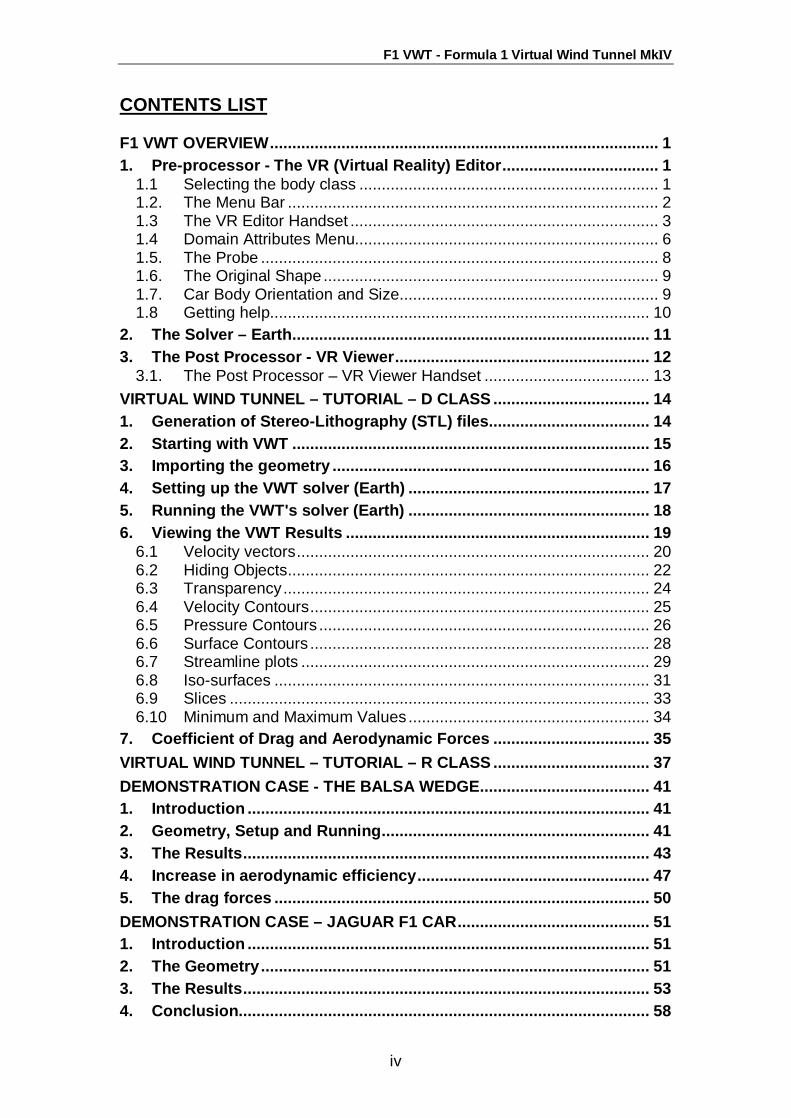
F1 VWT Overview 1. Pre-processor - The VR (Virtual Reality) Editor The Pre-processor is the part of the CFD program that sets up the aerodynamic test on the F1 model. From the desktop, click on the VWT icon
. Once initiated, the first screen should show a red-outlined (Domain) box with the default F1 balsa wood model. Everything in the VWT is created within this area and defines the limit of the space allocated.
1.1 Selecting the body class The body class can only be selected when starting a new case – it cannot be changed part way through a set up. To start a new case, click
• File ⇒ Start new case on the menu bar. From the dialog that appears, choose F1-D for the D-class body or F1-R for an R-class body. The examples in this guide are for a D-class body, but the methods used are identical for the two classes. The title F1 VWT (D) in the bottom-left corner of the image indicates that this is a D-class model.
Outlet
Inlet
Menu bar
Original shape
VR handset Road
Probe
F1 VWT - Formula 1 Virtual Wind Tunnel MkΙV
2
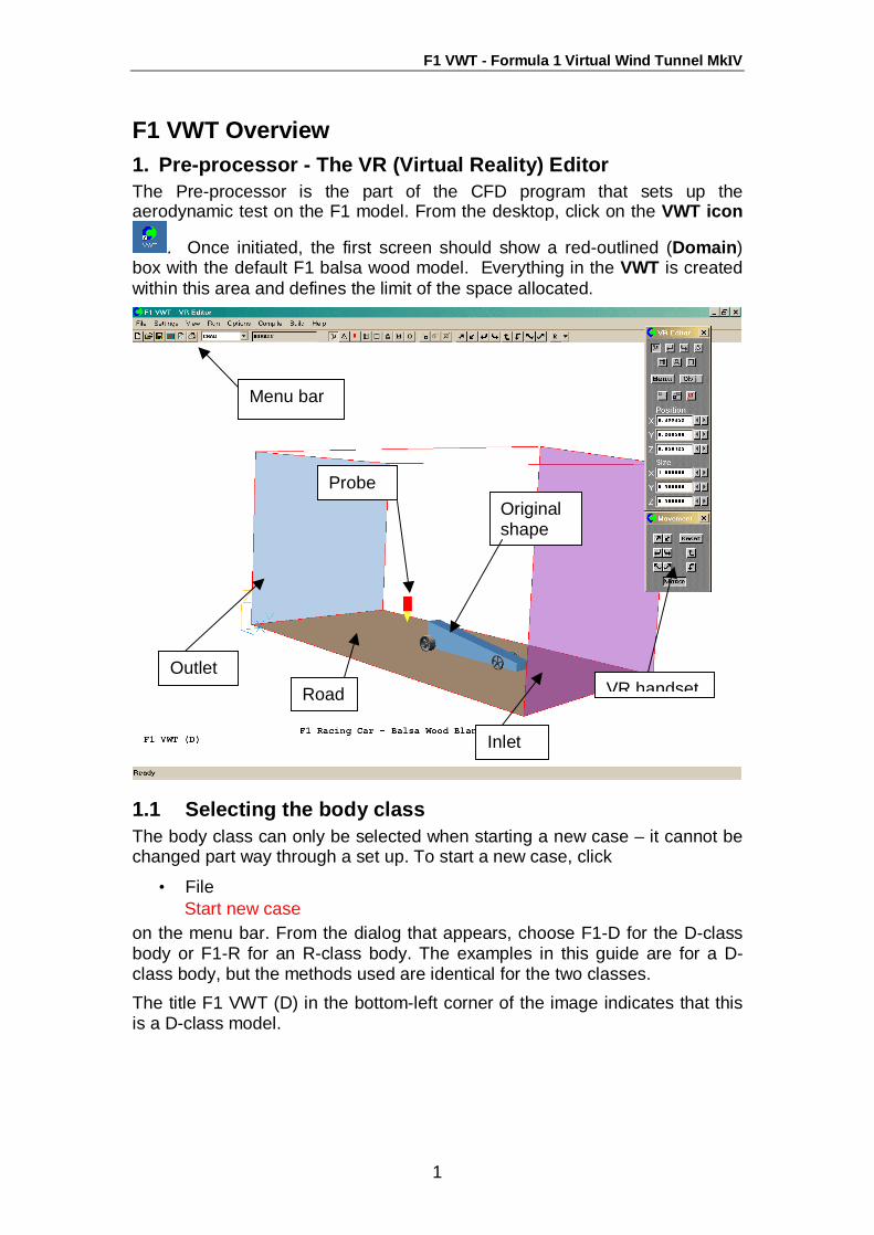
The balsa blank for the R-class looks like this.
Note that the title in the bottom-left corner is now F1 VWT (R).
1.2. The Menu Bar This gives access to everything in the VWT, but there are only certain important functions needed for the F1 in Schools Challenge. Everything else can be accessed from the ‘VR Handset’. Menu Bar File…
⇒ Open existing case Allows the opening of a previous simulation ⇒ Save as a case Saves the current simulation ⇒ Save window as Allows a screen shot in .GIF, BMP or PCX format ⇒ Exit Close down VWT Run…
⇒ Solver Runs the solver ⇒ Post-processor Runs the post-processor ⇒ Pre-processor Runs the pre-processor Options…
⇒ Change working directory Change to a preferred directory Note: The other options present in the menu bar should only be investigated in the presence of a teacher.
F1 VWT - Formula 1 Virtual Wind Tunnel MkΙV
3
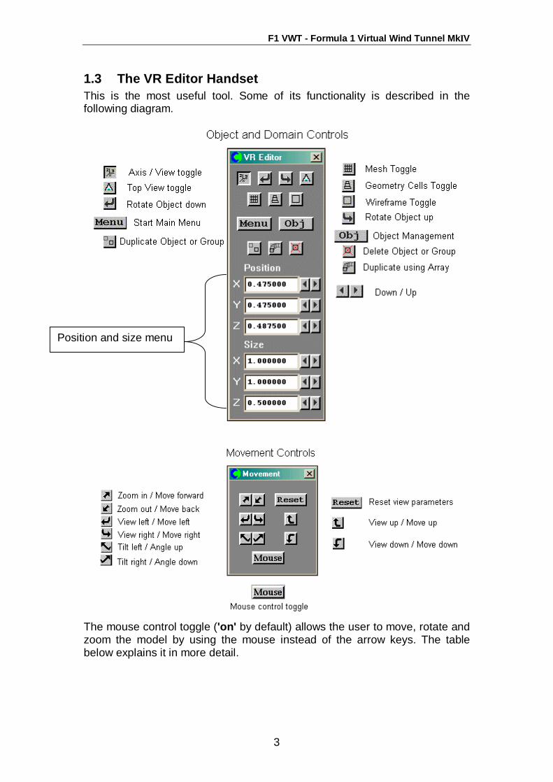
1.3 The VR Editor Handset This is the most useful tool. Some of its functionality is described in the following diagram.
The mouse control toggle ('on' by default) allows the user to move, rotate and zoom the model by using the mouse instead of the arrow keys. The table below explains it in more detail.
Position and size menu

F1 VWT - Formula 1 Virtual Wind Tunnel MkΙV
4
Mouse button held down
Mouse movement Effect Equivalent key
Left View left left-click on Right View right left-click on Up View up left-click on
Left
Down View down left-click on Left Tilt right left-click on Right Tilt left left-click on Up Zoom out left-click on
Right
Down Zoom in left-click on Left Move left right-click on Right Move right right-click on Up Move down right-click on
Middle (or both)
Down Move up right-click on
Left Rotate image right about viewer None
Right Rotate image left about viewer None
Up Rotate image down about viewer None
Shift+Left
Down Rotate image up about viewer None
Left None None Right None None Up Move back right-click on Shift+right
Down Move forward right-click on Quick Zoom To zoom into a region without panning and dragging, place the cursor where the centre of the zoomed image is to be. Press the control key <ctrl>, and with it held down, hold the left mouse button down and move the cursor to the left or right. A box will follow the movement of the cursor. When the mouse button is released while the control key is down, the area within the box will be expanded to fill the screen.
F1 VWT - Formula 1 Virtual Wind Tunnel MkΙV
5
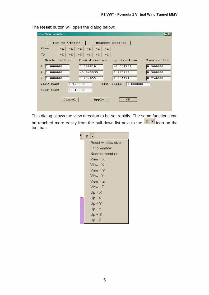
The Reset button will open the dialog below:
This dialog allows the view direction to be set rapidly. The same functions can be reached more easily from the pull-down list next to the icon on the tool bar:
F1 VWT - Formula 1 Virtual Wind Tunnel MkΙV
6
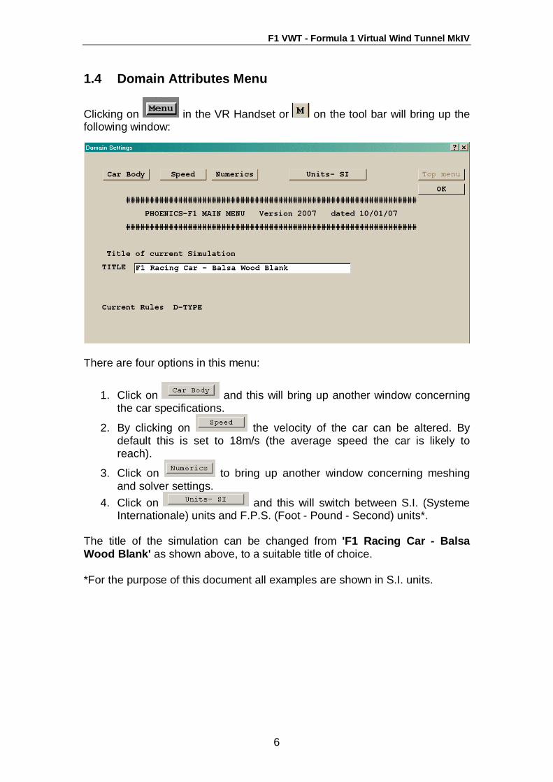
1.4 Domain Attributes Menu
Clicking on in the VR Handset or on the tool bar will bring up the following window:
There are four options in this menu:
1. Click on and this will bring up another window concerning the car specifications.
2. By clicking on the velocity of the car can be altered. By default this is set to 18m/s (the average speed the car is likely to reach).
3. Click on to bring up another window concerning meshing and solver settings.
4. Click on and this will switch between S.I. (Systeme Internationale) units and F.P.S. (Foot - Pound - Second) units*.
The title of the simulation can be changed from 'F1 Racing Car - Balsa Wood Blank' as shown above, to a suitable title of choice. *For the purpose of this document all examples are shown in S.I. units.
F1 VWT - Formula 1 Virtual Wind Tunnel MkΙV
7
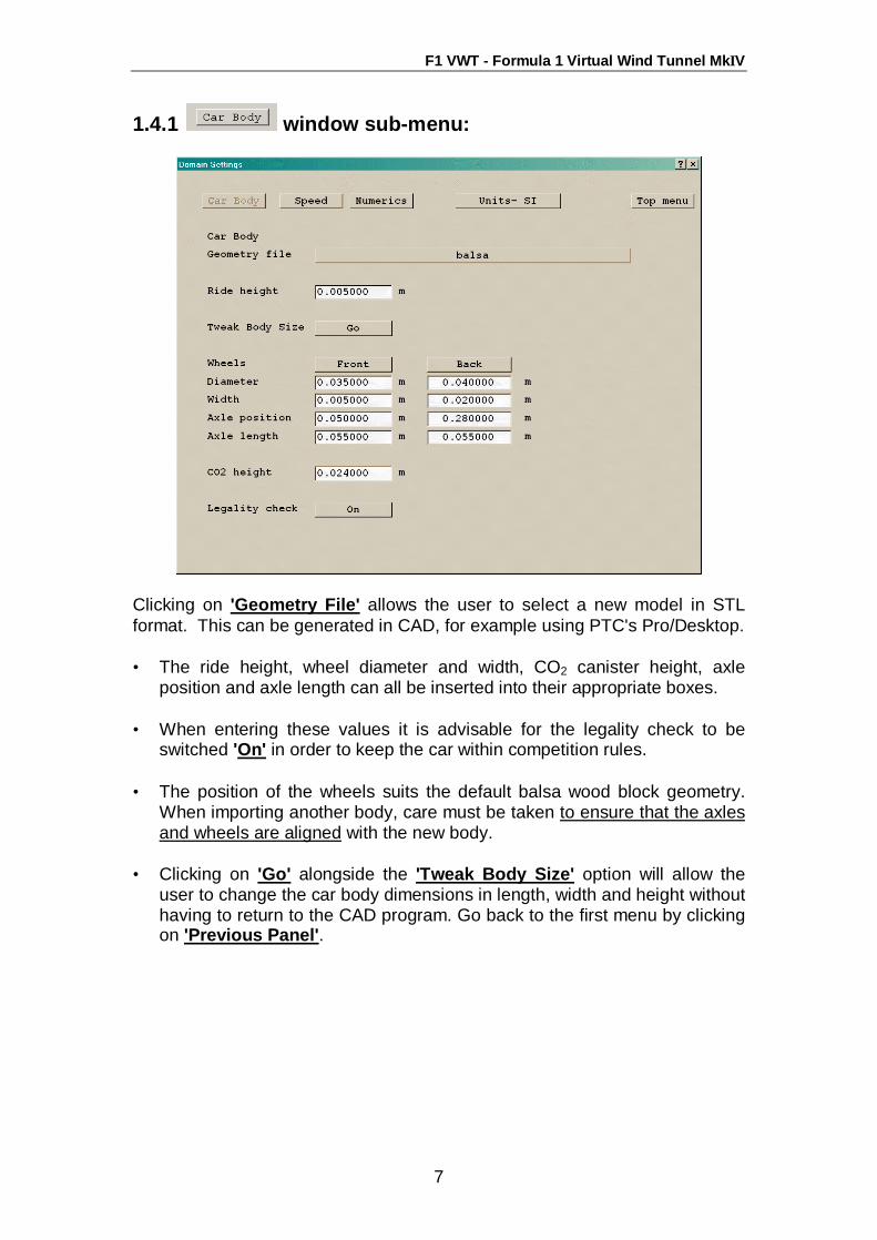
1.4.1 window sub-menu:
Clicking on 'Geometry File' allows the user to select a new model in STL format. This can be generated in CAD, for example using PTC's Pro/Desktop. • The ride height, wheel diameter and width, CO2 canister height, axle
position and axle length can all be inserted into their appropriate boxes. • When entering these values it is advisable for the legality check to be
switched 'On' in order to keep the car within competition rules. • The position of the wheels suits the default balsa wood block geometry.
When importing another body, care must be taken to ensure that the axles and wheels are aligned with the new body.
• Clicking on 'Go' alongside the 'Tweak Body Size' option will allow the
user to change the car body dimensions in length, width and height without having to return to the CAD program. Go back to the first menu by clicking on 'Previous Panel'.
F1 VWT - Formula 1 Virtual Wind Tunnel MkΙV
8
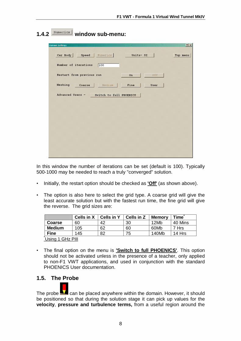
1.4.2 window sub-menu:
In this window the number of iterations can be set (default is 100). Typically 500-1000 may be needed to reach a truly "converged" solution. • Initially, the restart option should be checked as 'Off' (as shown above). • The option is also here to select the grid type. A coarse grid will give the
least accurate solution but with the fastest run time, the fine grid will give the reverse. The grid sizes are:
Cells in X Cells in Y Cells in Z Memory Time*
Coarse 60 42 30 12Mb 40 Mins Medium 105 62 60 60Mb 7 Hrs Fine 145 82 75 140Mb 14 Hrs
*Using 1 GHz PIII • The final option on the menu is 'Switch to full PHOENICS'. This option
should not be activated unless in the presence of a teacher, only applied to non-F1 VWT applications, and used in conjunction with the standard PHOENICS User documentation.
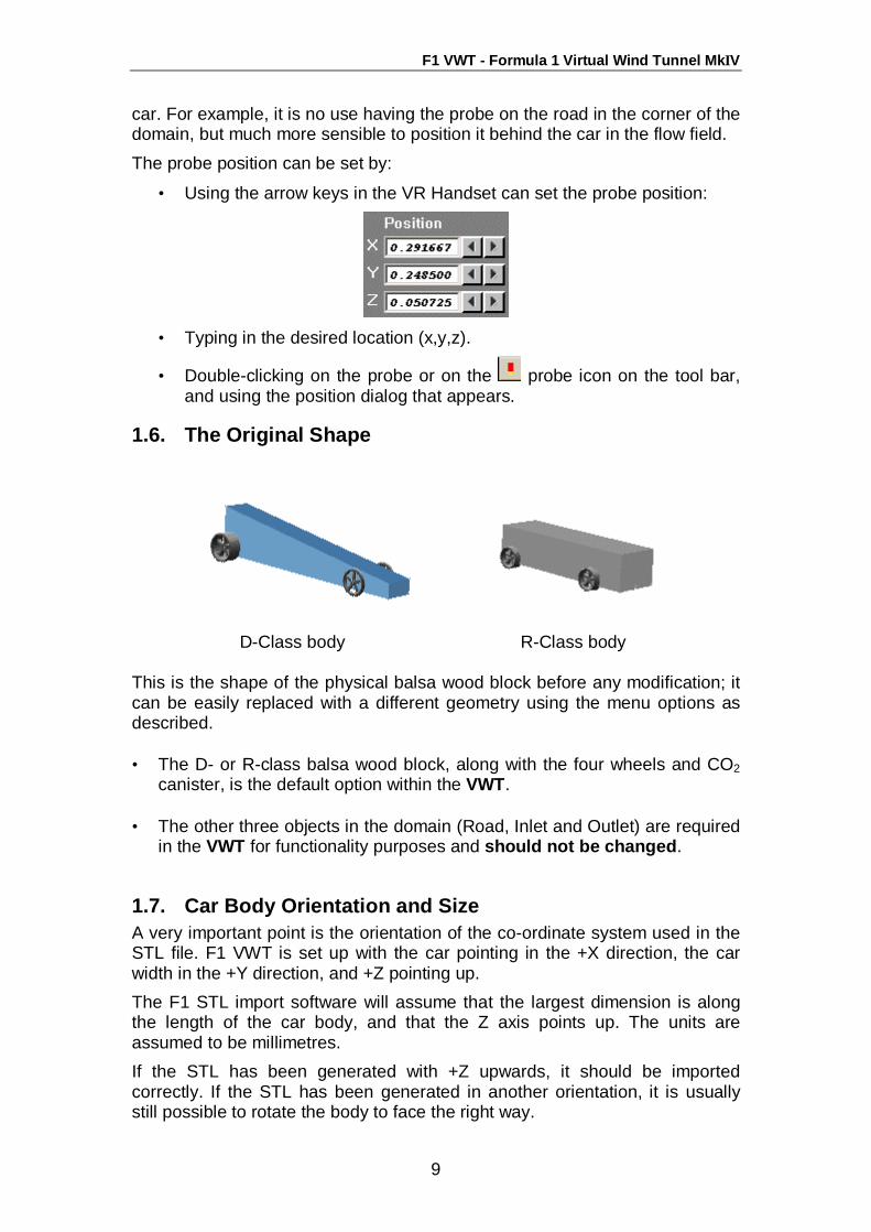
1.5. The Probe
The probe can be placed anywhere within the domain. However, it should be positioned so that during the solution stage it can pick up values for the velocity, pressure and turbulence terms, from a useful region around the
F1 VWT - Formula 1 Virtual Wind Tunnel MkΙV
9
car. For example, it is no use having the probe on the road in the corner of the domain, but much more sensible to position it behind the car in the flow field. The probe position can be set by:
• Using the arrow keys in the VR Handset can set the probe position:
• Typing in the desired location (x,y,z).
• Double-clicking on the probe or on the probe icon on the tool bar, and using the position dialog that appears.
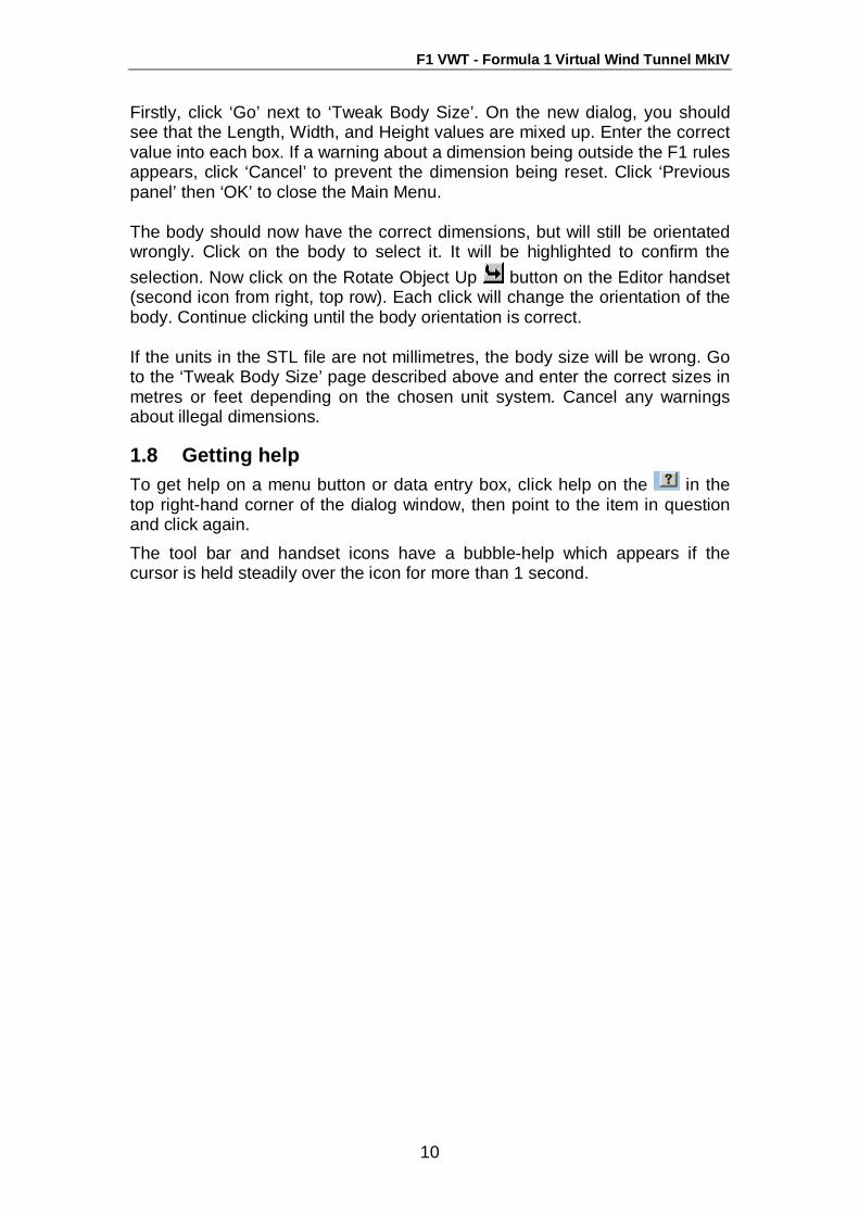
1.6. The Original Shape
D-Class body R-Class body This is the shape of the physical balsa wood block before any modification; it can be easily replaced with a different geometry using the menu options as described. • The D- or R-class balsa wood block, along with the four wheels and CO2
canister, is the default option within the VWT. • The other three objects in the domain (Road, Inlet and Outlet) are required
in the VWT for functionality purposes and should not be changed.
1.7. Car Body Orientation and Size A very important point is the orientation of the co-ordinate system used in the STL file. F1 VWT is set up with the car pointing in the +X direction, the car width in the +Y direction, and +Z pointing up. The F1 STL import software will assume that the largest dimension is along the length of the car body, and that the Z axis points up. The units are assumed to be millimetres. If the STL has been generated with +Z upwards, it should be imported correctly. If the STL has been generated in another orientation, it is usually still possible to rotate the body to face the right way.
F1 VWT - Formula 1 Virtual Wind Tunnel MkΙV
10
Firstly, click ‘Go’ next to ‘Tweak Body Size’. On the new dialog, you should see that the Length, Width, and Height values are mixed up. Enter the correct value into each box. If a warning about a dimension being outside the F1 rules appears, click ‘Cancel’ to prevent the dimension being reset. Click ‘Previous panel’ then ‘OK’ to close the Main Menu. The body should now have the correct dimensions, but will still be orientated wrongly. Click on the body to select it. It will be highlighted to confirm the selection. Now click on the Rotate Object Up button on the Editor handset (second icon from right, top row). Each click will change the orientation of the body. Continue clicking until the body orientation is correct. If the units in the STL file are not millimetres, the body size will be wrong. Go to the ‘Tweak Body Size’ page described above and enter the correct sizes in metres or feet depending on the chosen unit system. Cancel any warnings about illegal dimensions.
1.8 Getting help To get help on a menu button or data entry box, click help on the in the top right-hand corner of the dialog window, then point to the item in question and click again. The tool bar and handset icons have a bubble-help which appears if the cursor is held steadily over the icon for more than 1 second.
F1 VWT - Formula 1 Virtual Wind Tunnel MkΙV
11
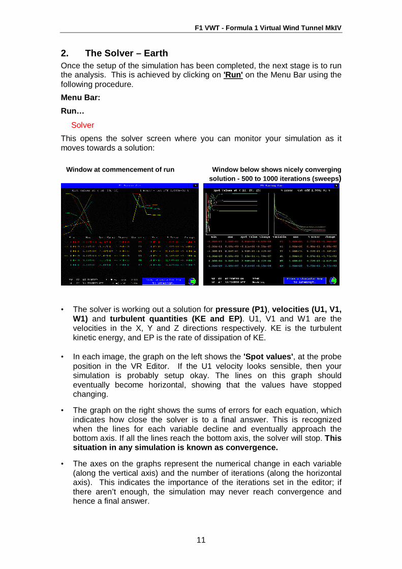
2. The Solver – Earth Once the setup of the simulation has been completed, the next stage is to run the analysis. This is achieved by clicking on 'Run' on the Menu Bar using the following procedure. Menu Bar: Run…
⇒ Solver This opens the solver screen where you can monitor your simulation as it moves towards a solution:
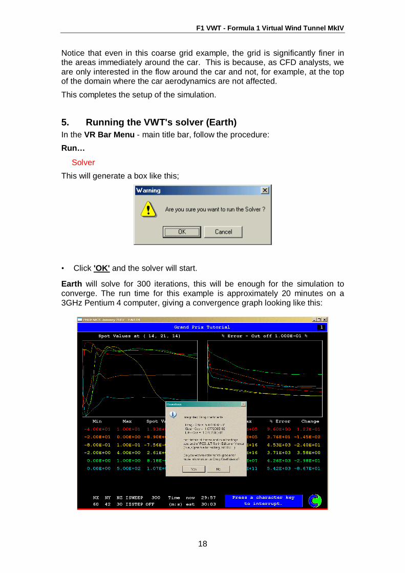
Window at commencement of run Window below shows nicely converging solution - 500 to 1000 iterations (sweeps)
• The solver is working out a solution for pressure (P1), velocities (U1, V1,
W1) and turbulent quantities (KE and EP). U1, V1 and W1 are the velocities in the X, Y and Z directions respectively. KE is the turbulent kinetic energy, and EP is the rate of dissipation of KE.
• In each image, the graph on the left shows the 'Spot values', at the probe
position in the VR Editor. If the U1 velocity looks sensible, then your simulation is probably setup okay. The lines on this graph should eventually become horizontal, showing that the values have stopped changing.
• The graph on the right shows the sums of errors for each equation, which indicates how close the solver is to a final answer. This is recognized when the lines for each variable decline and eventually approach the bottom axis. If all the lines reach the bottom axis, the solver will stop. This situation in any simulation is known as convergence.
• The axes on the graphs represent the numerical change in each variable
(along the vertical axis) and the number of iterations (along the horizontal axis). This indicates the importance of the iterations set in the editor; if there aren’t enough, the simulation may never reach convergence and hence a final answer.
F1 VWT - Formula 1 Virtual Wind Tunnel MkΙV
12
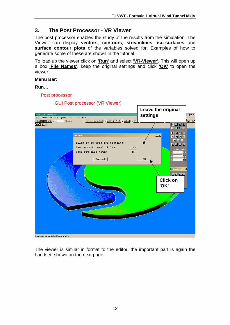
3. The Post Processor - VR Viewer The post processor enables the study of the results from the simulation. The Viewer can display vectors, contours, streamlines, iso-surfaces and surface contour plots of the variables solved for. Examples of how to generate some of these are shown in the tutorial. To load up the viewer click on 'Run' and select 'VR-Viewer', This will open up a box 'File Names', keep the original settings and click 'OK' to open the viewer. Menu Bar: Run…
⇒ Post processor
⇒ GUI Post processor (VR Viewer)
The viewer is similar in format to the editor; the important part is again the handset, shown on the next page.
Click on 'OK'
Leave the original settings
F1 VWT - Formula 1 Virtual Wind Tunnel MkΙV
13
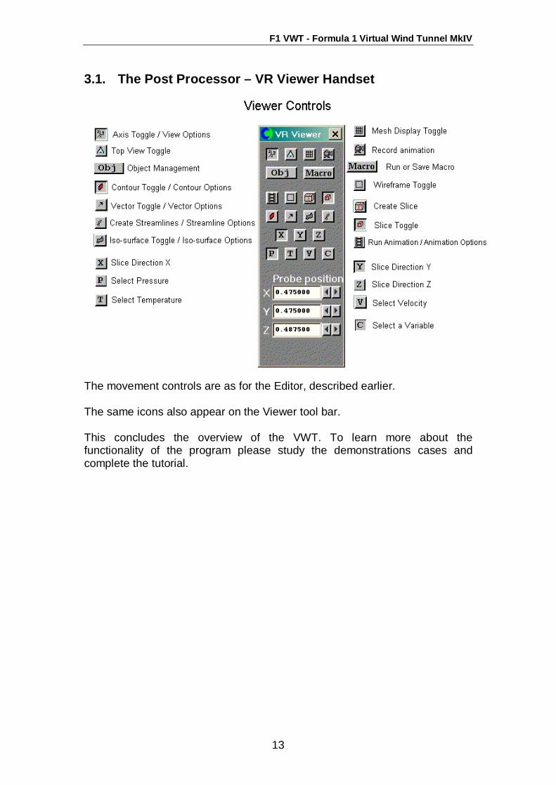
3.1. The Post Processor – VR Viewer Handset
The movement controls are as for the Editor, described earlier. The same icons also appear on the Viewer tool bar.
This concludes the overview of the VWT. To learn more about the functionality of the program please study the demonstrations cases and complete the tutorial.
F1 VWT - Formula 1 Virtual Wind Tunnel MkΙV
14
Virtual Wind Tunnel – Tutorial – D Class This tutorial follows on from PTC's ‘Grand Prix 2000ii 2D’ Pro/Desktop tutorial. Within this session the functionality of the Virtual Wind Tunnel (VWT) will be demonstrated from exporting suitable car geometries from Pro/Desktop, through obtaining a solution, to viewing the results generated. It is recommended that the user read ‘VWT Overview’ before starting this tutorial.
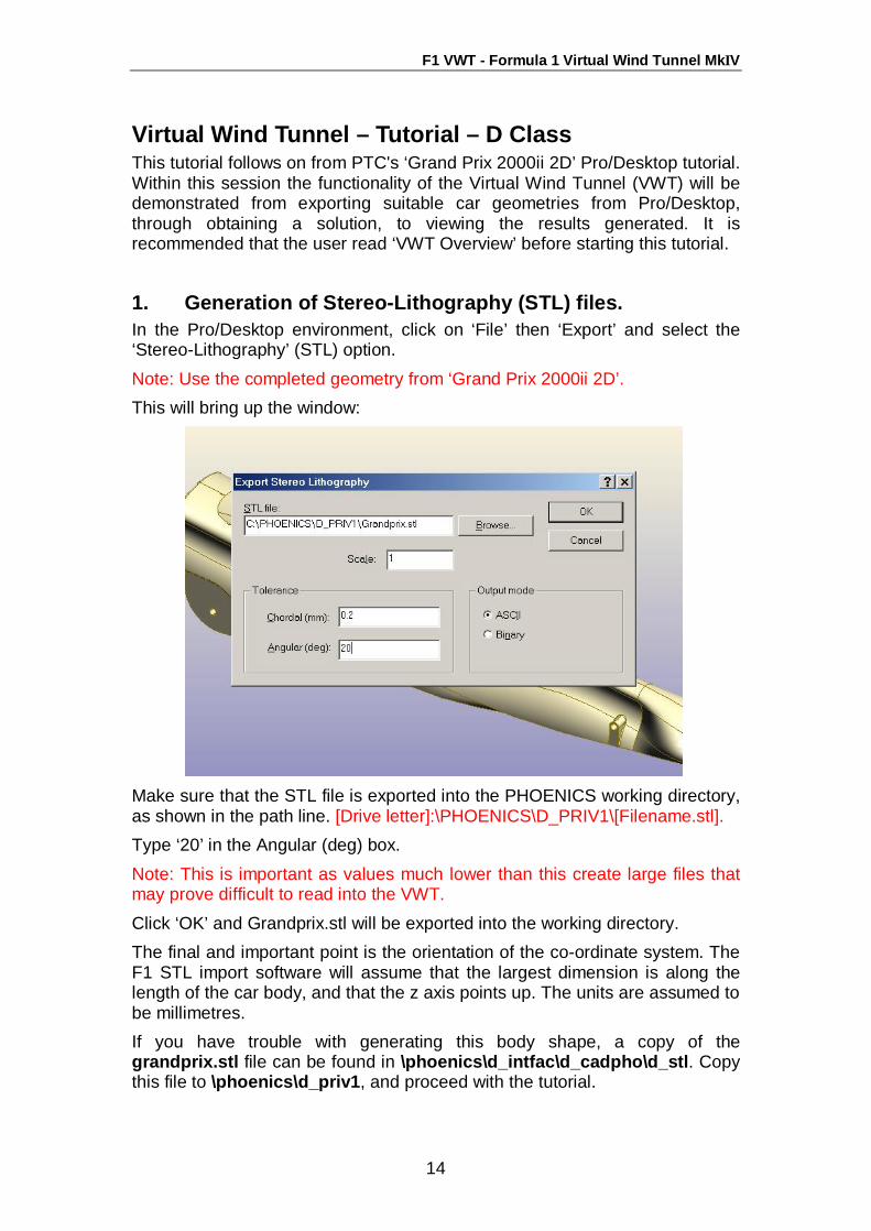
1. Generation of Stereo-Lithography (STL) files. In the Pro/Desktop environment, click on ‘File’ then ‘Export’ and select the ‘Stereo-Lithography’ (STL) option. Note: Use the completed geometry from ‘Grand Prix 2000ii 2D’. This will bring up the window:
Make sure that the STL file is exported into the PHOENICS working directory, as shown in the path line. [Drive letter]:\PHOENICS\D_PRIV1\[Filename.stl]. Type ‘20’ in the Angular (deg) box. Note: This is important as values much lower than this create large files that may prove difficult to read into the VWT. Click ‘OK’ and Grandprix.stl will be exported into the working directory. The final and important point is the orientation of the co-ordinate system. The F1 STL import software will assume that the largest dimension is along the length of the car body, and that the z axis points up. The units are assumed to be millimetres. If you have trouble with generating this body shape, a copy of the grandprix.stl file can be found in \phoenics\d_intfac\d_cadpho\d_stl. Copy this file to \phoenics\d_priv1, and proceed with the tutorial.
F1 VWT - Formula 1 Virtual Wind Tunnel MkΙV
15
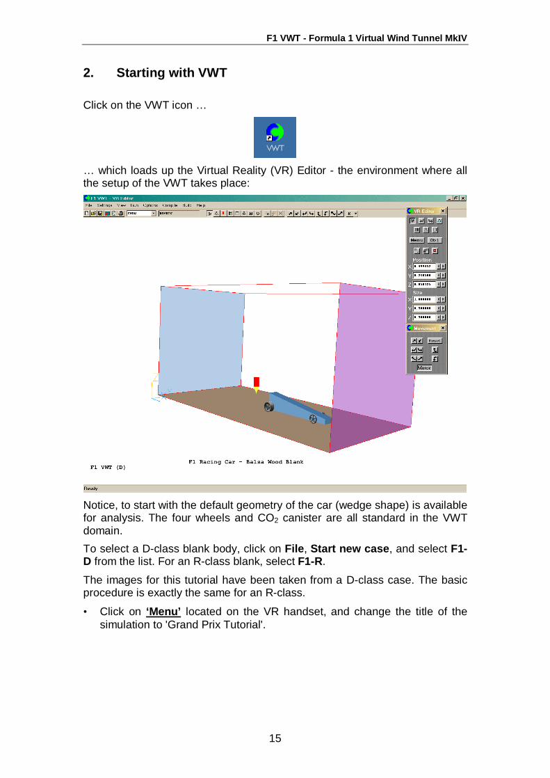
2. Starting with VWT Click on the VWT icon …
… which loads up the Virtual Reality (VR) Editor - the environment where all the setup of the VWT takes place:
Notice, to start with the default geometry of the car (wedge shape) is available for analysis. The four wheels and CO2 canister are all standard in the VWT domain. To select a D-class blank body, click on File, Start new case, and select F1-D from the list. For an R-class blank, select F1-R.
The images for this tutorial have been taken from a D-class case. The basic procedure is exactly the same for an R-class.
• Click on ‘Menu’ located on the VR handset, and change the title of the simulation to 'Grand Prix Tutorial'.
F1 VWT - Formula 1 Virtual Wind Tunnel MkΙV
16
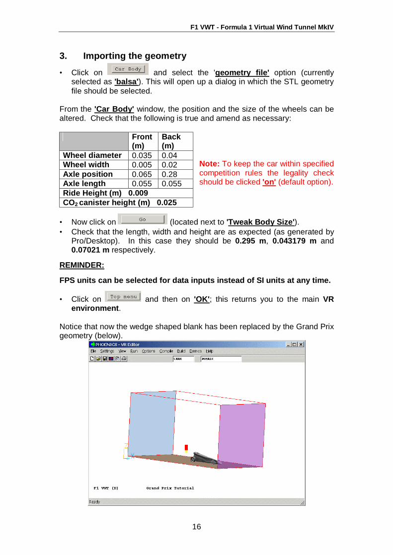
3. Importing the geometry
• Click on and select the 'geometry file' option (currently selected as 'balsa'). This will open up a dialog in which the STL geometry file should be selected.
From the 'Car Body' window, the position and the size of the wheels can be altered. Check that the following is true and amend as necessary:
Note: To keep the car within specified competition rules the legality check should be clicked 'on' (default option).
• Now click on (located next to 'Tweak Body Size'). • Check that the length, width and height are as expected (as generated by
Pro/Desktop). In this case they should be 0.295 m, 0.043179 m and 0.07021 m respectively.
REMINDER: FPS units can be selected for data inputs instead of SI units at any time.
• Click on and then on 'OK'; this returns you to the main VR environment.
Notice that now the wedge shaped blank has been replaced by the Grand Prix geometry (below).
Front (m)
Back (m)
Wheel diameter 0.035 0.04 Wheel width 0.005 0.02 Axle position 0.065 0.28 Axle length 0.055 0.055 Ride Height (m) 0.009 CO2 canister height (m) 0.025
F1 VWT - Formula 1 Virtual Wind Tunnel MkΙV
17
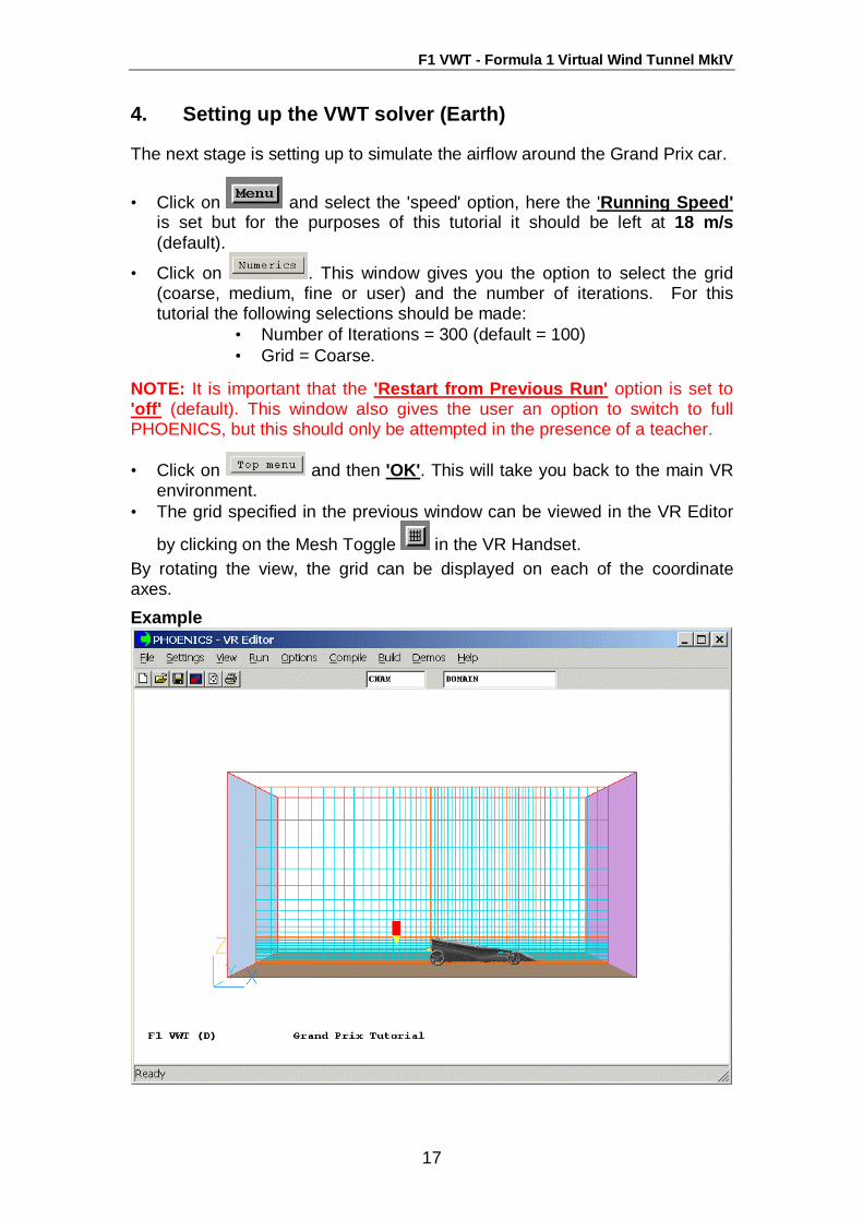
4. Setting up the VWT solver (Earth) The next stage is setting up to simulate the airflow around the Grand Prix car.
• Click on and select the 'speed' option, here the 'Running Speed' is set but for the purposes of this tutorial it should be left at 18 m/s (default).
• Click on . This window gives you the option to select the grid (coarse, medium, fine or user) and the number of iterations. For this tutorial the following selections should be made:
• Number of Iterations = 300 (default = 100) • Grid = Coarse.
NOTE: It is important that the 'Restart from Previous Run' option is set to 'off' (default). This window also gives the user an option to switch to full PHOENICS, but this should only be attempted in the presence of a teacher.
• Click on and then 'OK'. This will take you back to the main VR environment.
• The grid specified in the previous window can be viewed in the VR Editor
by clicking on the Mesh Toggle in the VR Handset. By rotating the view, the grid can be displayed on each of the coordinate axes. Example
F1 VWT - Formula 1 Virtual Wind Tunnel MkΙV
18
Notice that even in this coarse grid example, the grid is significantly finer in the areas immediately around the car. This is because, as CFD analysts, we are only interested in the flow around the car and not, for example, at the top of the domain where the car aerodynamics are not affected. This completes the setup of the simulation.
5. Running the VWT's solver (Earth) In the VR Bar Menu - main title bar, follow the procedure: Run…
⇒ Solver This will generate a box like this;
• Click 'OK' and the solver will start. Earth will solve for 300 iterations, this will be enough for the simulation to converge. The run time for this example is approximately 20 minutes on a 3GHz Pentium 4 computer, giving a convergence graph looking like this:
F1 VWT - Formula 1 Virtual Wind Tunnel MkΙV
19
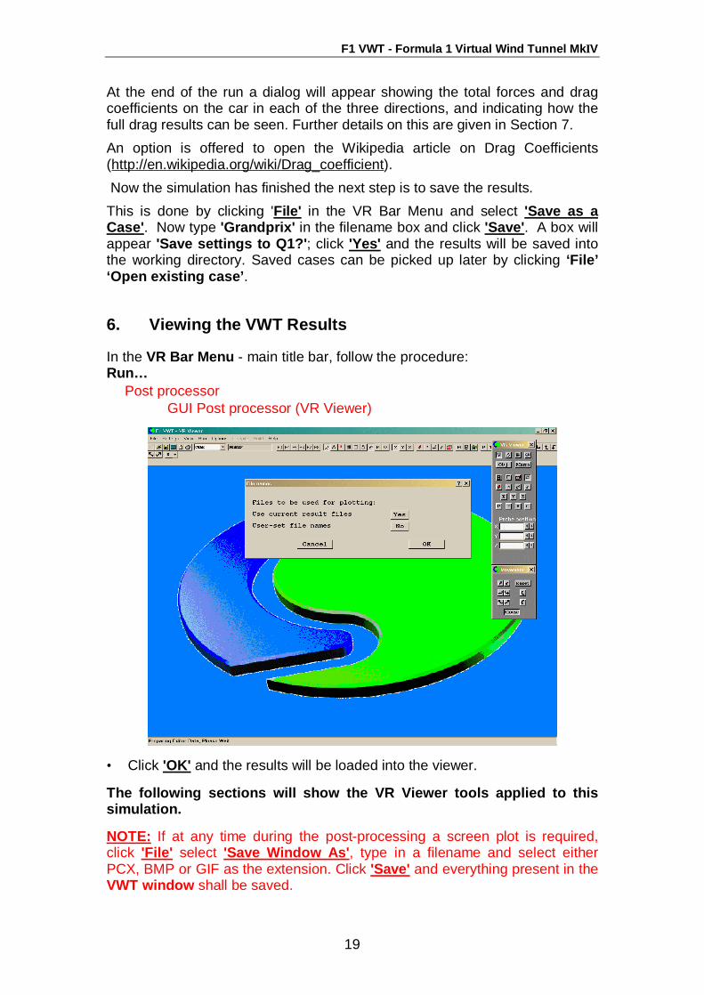
At the end of the run a dialog will appear showing the total forces and drag coefficients on the car in each of the three directions, and indicating how the full drag results can be seen. Further details on this are given in Section 7. An option is offered to open the Wikipedia article on Drag Coefficients (http://en.wikipedia.org/wiki/Drag_coefficient). Now the simulation has finished the next step is to save the results. This is done by clicking 'File' in the VR Bar Menu and select 'Save as a Case'. Now type 'Grandprix' in the filename box and click 'Save'. A box will appear 'Save settings to Q1?'; click 'Yes' and the results will be saved into the working directory. Saved cases can be picked up later by clicking ‘File’ ‘Open existing case’.
6. Viewing the VWT Results In the VR Bar Menu - main title bar, follow the procedure: Run… ⇒ Post processor
⇒ GUI Post processor (VR Viewer)
• Click 'OK' and the results will be loaded into the viewer. The following sections will show the VR Viewer tools applied to this simulation. NOTE: If at any time during the post-processing a screen plot is required, click 'File' select 'Save Window As', type in a filename and select either PCX, BMP or GIF as the extension. Click 'Save' and everything present in the VWT window shall be saved.
F1 VWT - Formula 1 Virtual Wind Tunnel MkΙV
20
The results of the simulation can be visualized as:
• Vectors (arrows showing local flow speed and direction).
• Contour maps showing distributions of pressure or velocity at selected planes.
• Iso-surfaces showing regions of constant value.
• Streamlines showing the path of dust particles dropped at chosen locations.
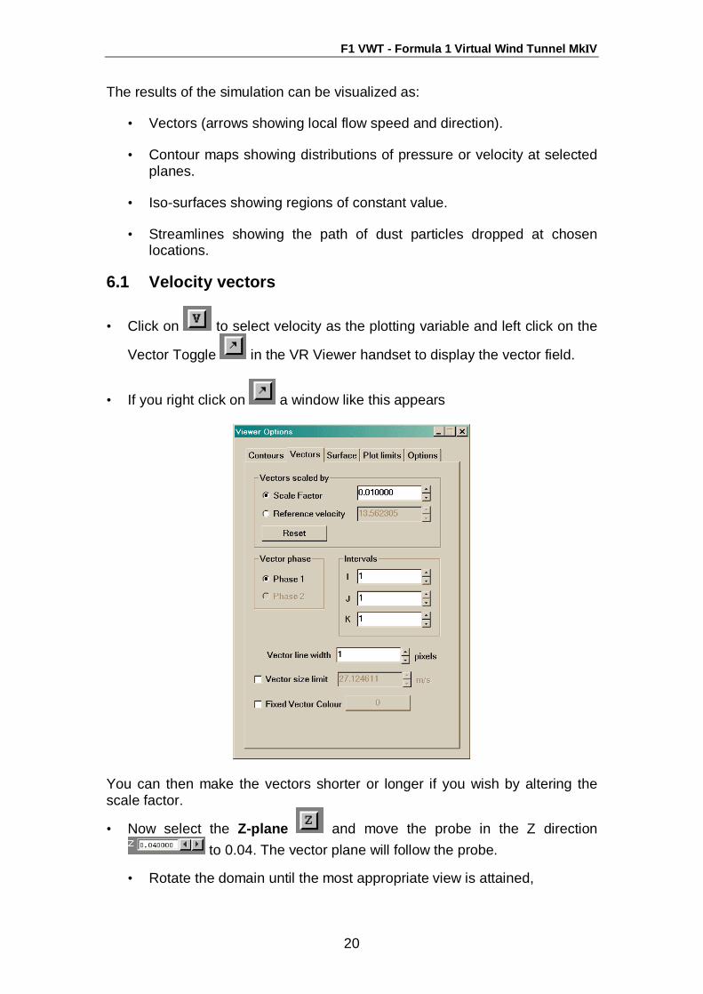
6.1 Velocity vectors
• Click on to select velocity as the plotting variable and left click on the
Vector Toggle in the VR Viewer handset to display the vector field.
• If you right click on a window like this appears
You can then make the vectors shorter or longer if you wish by altering the scale factor.
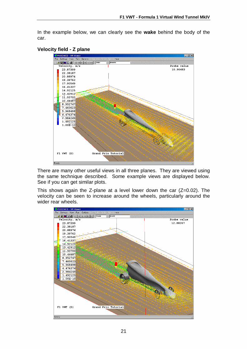
• Now select the Z-plane and move the probe in the Z direction to 0.04. The vector plane will follow the probe.
• Rotate the domain until the most appropriate view is attained,
F1 VWT - Formula 1 Virtual Wind Tunnel MkΙV
21
In the example below, we can clearly see the wake behind the body of the car. Velocity field - Z plane
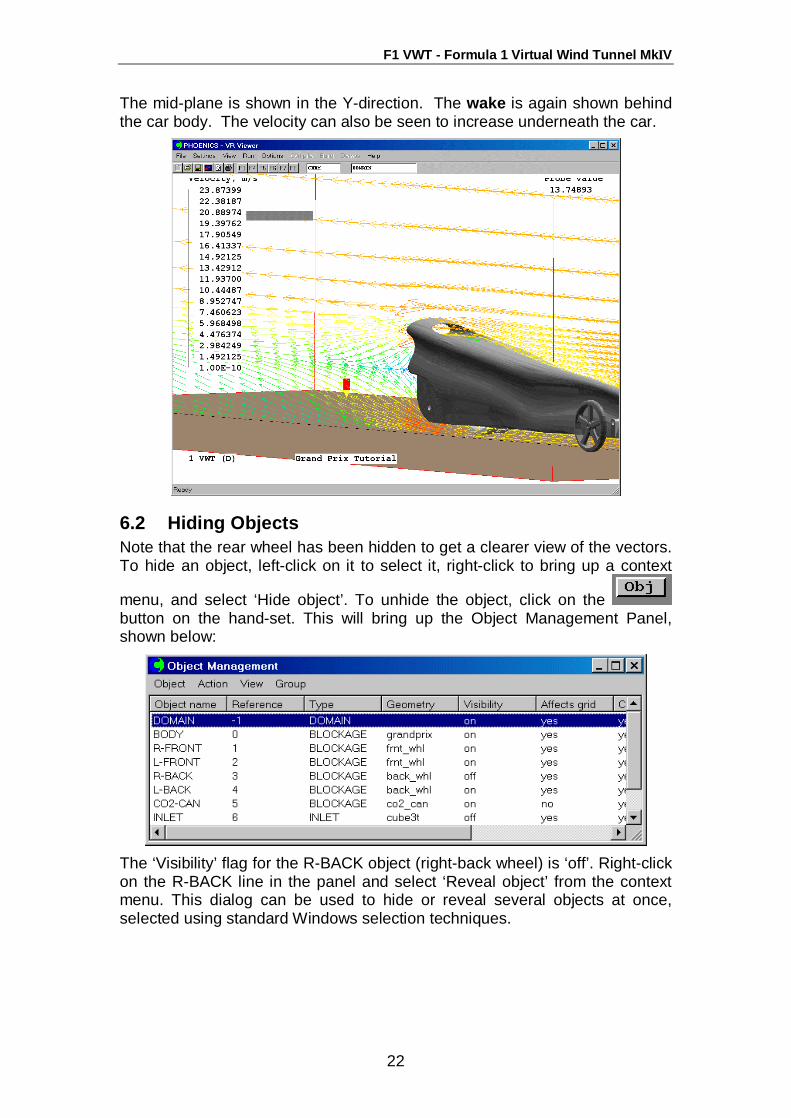
There are many other useful views in all three planes. They are viewed using the same technique described. Some example views are displayed below. See if you can get similar plots. This shows again the Z-plane at a level lower down the car (Z=0.02). The velocity can be seen to increase around the wheels, particularly around the wider rear wheels.
F1 VWT - Formula 1 Virtual Wind Tunnel MkΙV
22
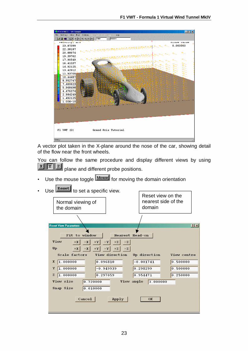
The mid-plane is shown in the Y-direction. The wake is again shown behind the car body. The velocity can also be seen to increase underneath the car.
6.2 Hiding Objects Note that the rear wheel has been hidden to get a clearer view of the vectors. To hide an object, left-click on it to select it, right-click to bring up a context
menu, and select ‘Hide object’. To unhide the object, click on the button on the hand-set. This will bring up the Object Management Panel, shown below:
The ‘Visibility’ flag for the R-BACK object (right-back wheel) is ‘off’. Right-click on the R-BACK line in the panel and select ‘Reveal object’ from the context menu. This dialog can be used to hide or reveal several objects at once, selected using standard Windows selection techniques.
F1 VWT - Formula 1 Virtual Wind Tunnel MkΙV
23
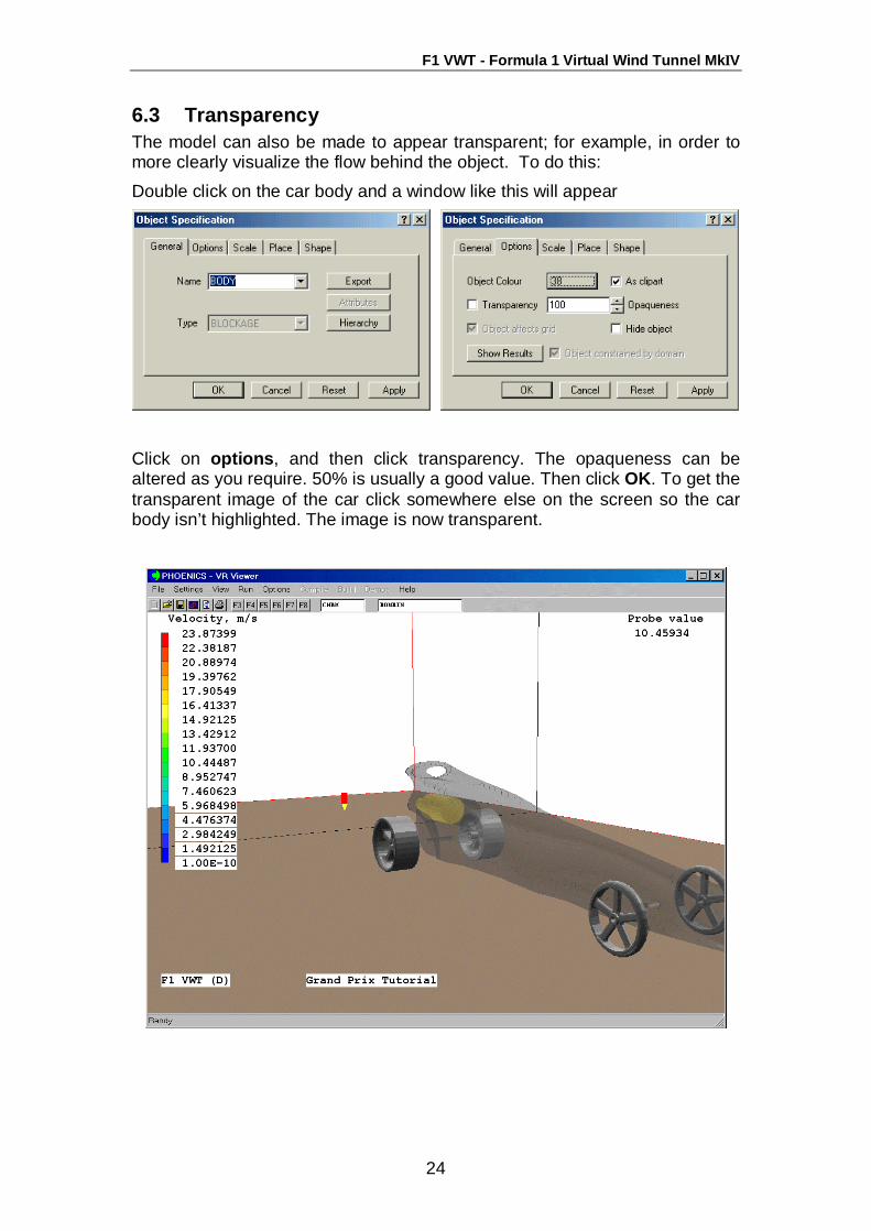
A vector plot taken in the X-plane around the nose of the car, showing detail of the flow near the front wheels. You can follow the same procedure and display different views by using
plane and different probe positions.
• Use the mouse toggle for moving the domain orientation
• Use to set a specific view.
Reset view on the nearest side of the domain
Normal viewing of the domain
F1 VWT - Formula 1 Virtual Wind Tunnel MkΙV
24
6.3 Transparency The model can also be made to appear transparent; for example, in order to more clearly visualize the flow behind the object. To do this: Double click on the car body and a window like this will appear
Click on options, and then click transparency. The opaqueness can be altered as you require. 50% is usually a good value. Then click OK. To get the transparent image of the car click somewhere else on the screen so the car body isn’t highlighted. The image is now transparent.
F1 VWT - Formula 1 Virtual Wind Tunnel MkΙV
25
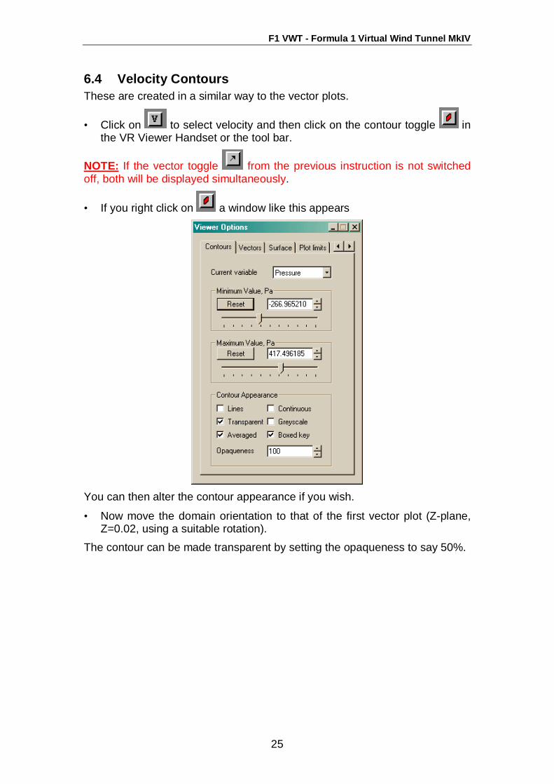
6.4 Velocity Contours These are created in a similar way to the vector plots.
• Click on to select velocity and then click on the contour toggle in the VR Viewer Handset or the tool bar.
NOTE: If the vector toggle from the previous instruction is not switched off, both will be displayed simultaneously.
• If you right click on a window like this appears
You can then alter the contour appearance if you wish.
• Now move the domain orientation to that of the first vector plot (Z-plane, Z=0.02, using a suitable rotation).
The contour can be made transparent by setting the opaqueness to say 50%.
F1 VWT - Formula 1 Virtual Wind Tunnel MkΙV
26
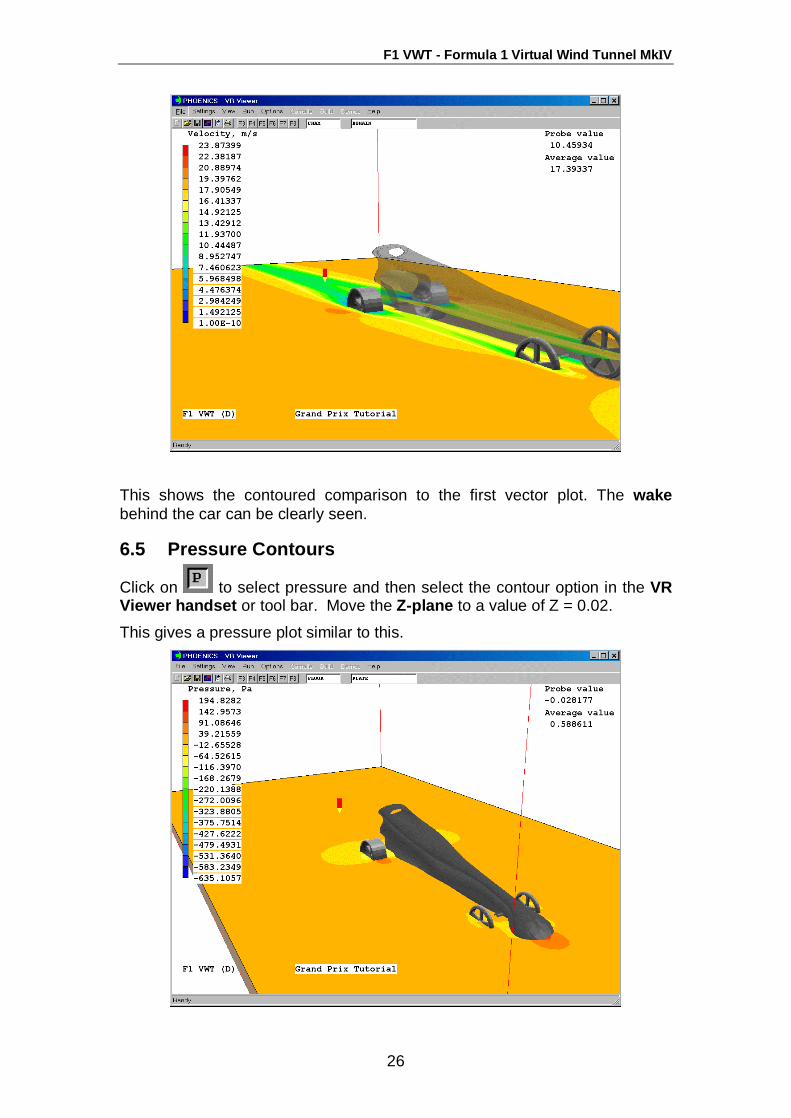
This shows the contoured comparison to the first vector plot. The wake behind the car can be clearly seen.
6.5 Pressure Contours
Click on to select pressure and then select the contour option in the VR Viewer handset or tool bar. Move the Z-plane to a value of Z = 0.02.
This gives a pressure plot similar to this.
F1 VWT - Formula 1 Virtual Wind Tunnel MkΙV
27
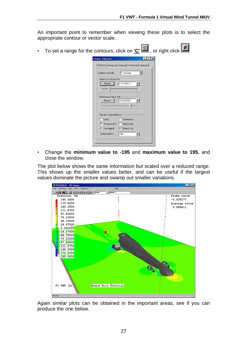
An important point to remember when viewing these plots is to select the appropriate contour or vector scale.
• To set a range for the contours, click on 'C' , or right click
• Change the minimum value to -195 and maximum value to 195, and
close the window. The plot below shows the same information but scaled over a reduced range. This shows up the smaller values better, and can be useful if the largest values dominate the picture and swamp out smaller variations.
Again similar plots can be obtained in the important areas, see if you can produce the one below.
F1 VWT - Formula 1 Virtual Wind Tunnel MkΙV
28
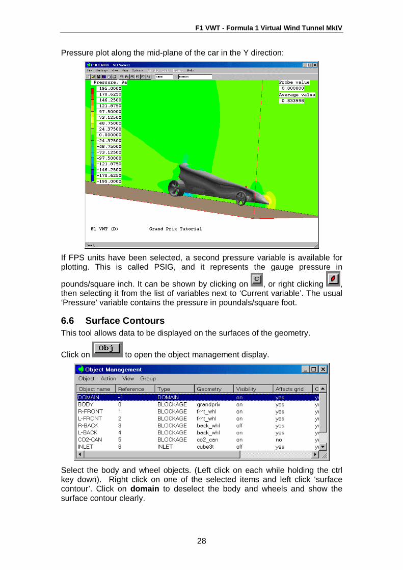
Pressure plot along the mid-plane of the car in the Y direction:
If FPS units have been selected, a second pressure variable is available for plotting. This is called PSIG, and it represents the gauge pressure in
pounds/square inch. It can be shown by clicking on , or right clicking , then selecting it from the list of variables next to ‘Current variable’. The usual ‘Pressure’ variable contains the pressure in poundals/square foot.
6.6 Surface Contours This tool allows data to be displayed on the surfaces of the geometry.
Click on to open the object management display.
Select the body and wheel objects. (Left click on each while holding the ctrl key down). Right click on one of the selected items and left click ‘surface contour’. Click on domain to deselect the body and wheels and show the surface contour clearly.
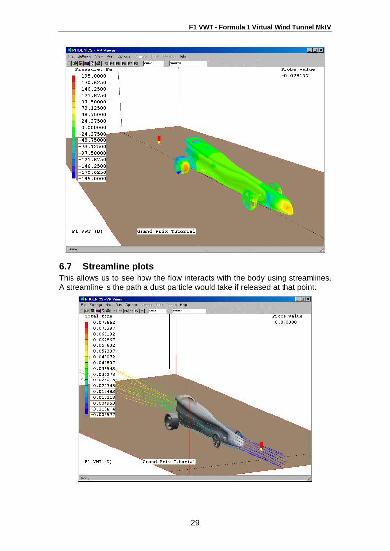
F1 VWT - Formula 1 Virtual Wind Tunnel MkΙV
29
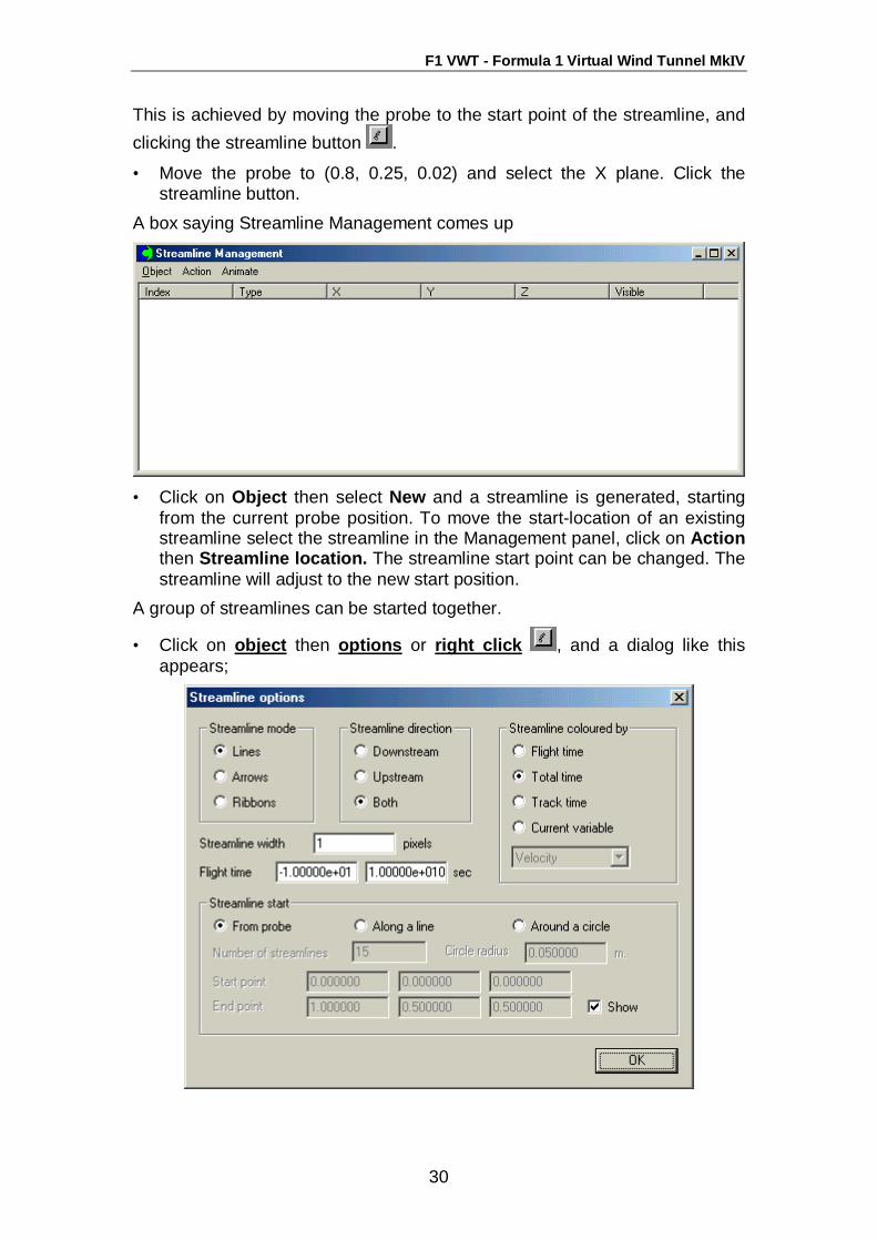
6.7 Streamline plots This allows us to see how the flow interacts with the body using streamlines. A streamline is the path a dust particle would take if released at that point.
F1 VWT - Formula 1 Virtual Wind Tunnel MkΙV
30
This is achieved by moving the probe to the start point of the streamline, and clicking the streamline button .
• Move the probe to (0.8, 0.25, 0.02) and select the X plane. Click the streamline button.
A box saying Streamline Management comes up
• Click on Object then select New and a streamline is generated, starting
from the current probe position. To move the start-location of an existing streamline select the streamline in the Management panel, click on Action then Streamline location. The streamline start point can be changed. The streamline will adjust to the new start position.
A group of streamlines can be started together.
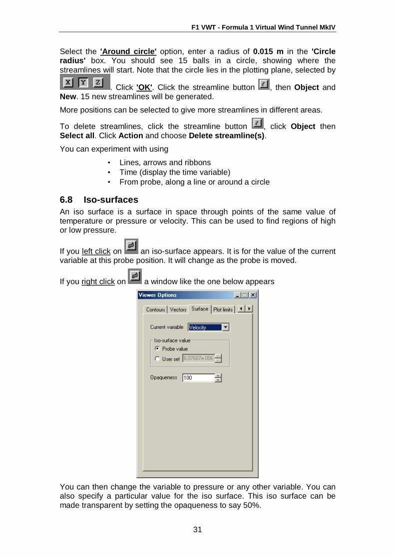
• Click on object then options or right click , and a dialog like this appears;
F1 VWT - Formula 1 Virtual Wind Tunnel MkΙV
31
Select the 'Around circle' option, enter a radius of 0.015 m in the 'Circle radius' box. You should see 15 balls in a circle, showing where the streamlines will start. Note that the circle lies in the plotting plane, selected by
. Click 'OK'. Click the streamline button , then Object and New. 15 new streamlines will be generated.
More positions can be selected to give more streamlines in different areas.
To delete streamlines, click the streamline button , click Object then Select all. Click Action and choose Delete streamline(s). You can experiment with using
• Lines, arrows and ribbons • Time (display the time variable) • From probe, along a line or around a circle
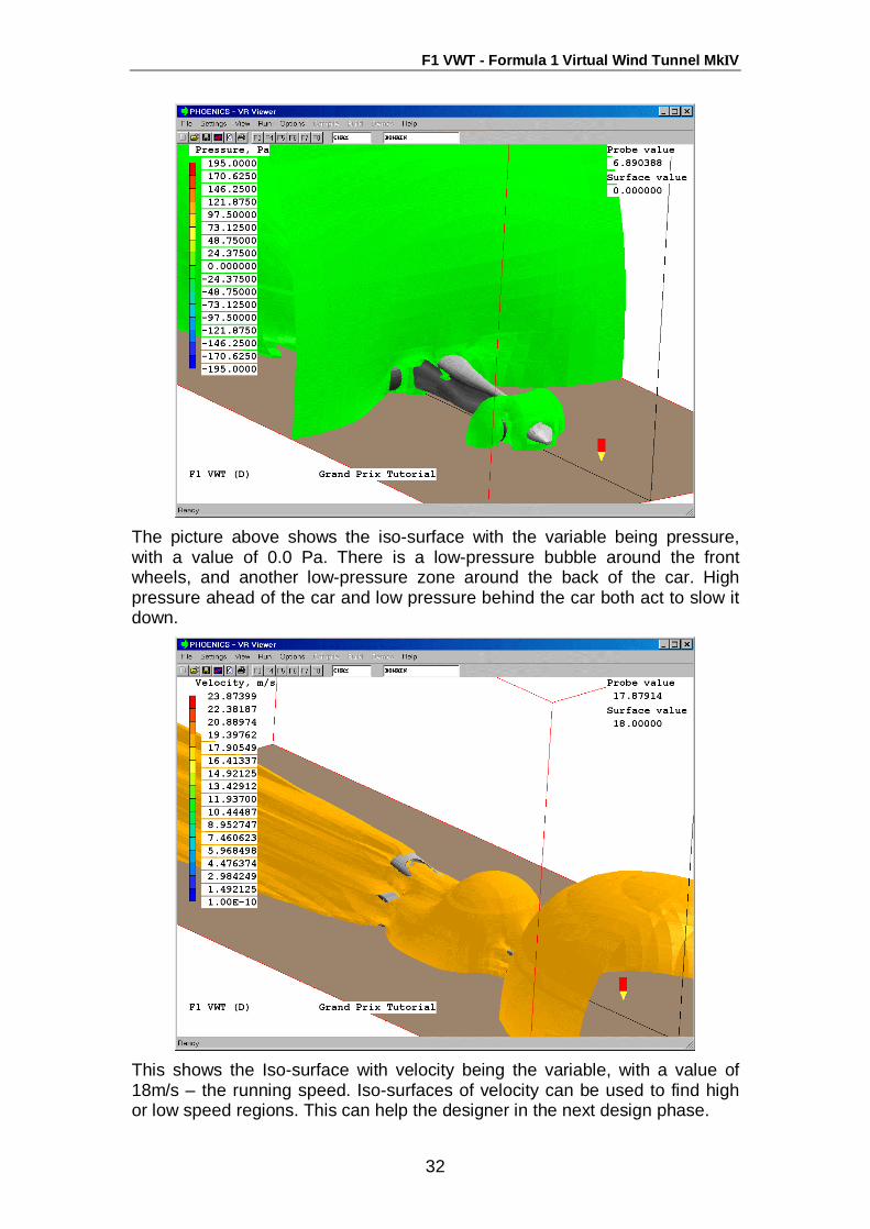
6.8 Iso-surfaces An iso surface is a surface in space through points of the same value of temperature or pressure or velocity. This can be used to find regions of high or low pressure.
If you left click on an iso-surface appears. It is for the value of the current variable at this probe position. It will change as the probe is moved.
If you right click on a window like the one below appears
You can then change the variable to pressure or any other variable. You can also specify a particular value for the iso surface. This iso surface can be made transparent by setting the opaqueness to say 50%.
F1 VWT - Formula 1 Virtual Wind Tunnel MkΙV
32
The picture above shows the iso-surface with the variable being pressure, with a value of 0.0 Pa. There is a low-pressure bubble around the front wheels, and another low-pressure zone around the back of the car. High pressure ahead of the car and low pressure behind the car both act to slow it down.
This shows the Iso-surface with velocity being the variable, with a value of 18m/s – the running speed. Iso-surfaces of velocity can be used to find high or low speed regions. This can help the designer in the next design phase.
F1 VWT - Formula 1 Virtual Wind Tunnel MkΙV
33
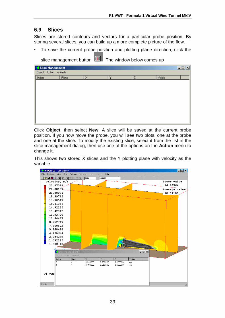
6.9 Slices Slices are stored contours and vectors for a particular probe position. By storing several slices, you can build up a more complete picture of the flow.
• To save the current probe position and plotting plane direction, click the
slice management button .The window below comes up
Click Object, then select New. A slice will be saved at the current probe position. If you now move the probe, you will see two plots, one at the probe and one at the slice. To modify the existing slice, select it from the list in the slice management dialog, then use one of the options on the Action menu to change it. This shows two stored X slices and the Y plotting plane with velocity as the variable.
.
F1 VWT - Formula 1 Virtual Wind Tunnel MkΙV
34
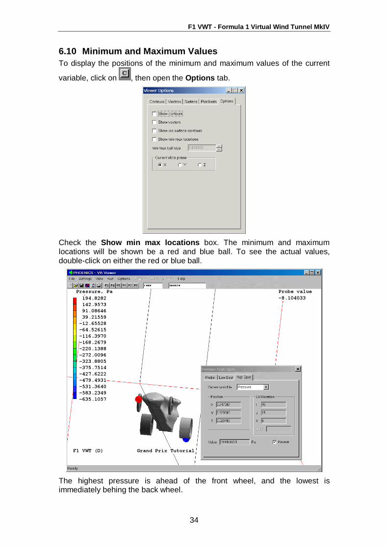
6.10 Minimum and Maximum Values To display the positions of the minimum and maximum values of the current
variable, click on , then open the Options tab.
Check the Show min max locations box. The minimum and maximum locations will be shown be a red and blue ball. To see the actual values, double-click on either the red or blue ball.
The highest pressure is ahead of the front wheel, and the lowest is immediately behing the back wheel.
F1 VWT - Formula 1 Virtual Wind Tunnel MkΙV
35
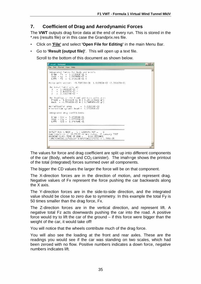
7. Coefficient of Drag and Aerodynamic Forces The VWT outputs drag force data at the end of every run. This is stored in the *.res (results file) or in this case the Grandprix.res file.
• Click on 'File' and select 'Open File for Editing' in the main Menu Bar.
• Go to 'Result (output file)'. This will open up a text file.
Scroll to the bottom of this document as shown below.
The values for force and drag coefficient are split up into different components of the car (Body, wheels and CO2 canister). The imah=ge shows the printout of the total (integrated) forces summed over all components. The bigger the CD values the larger the force will be on that component. The X-direction forces are in the direction of motion, and represent drag. Negative values of Fx represent the force pushing the car backwards along the X axis. The Y-direction forces are in the side-to-side direction, and the integrated value should be close to zero due to symmetry. In this example the total Fy is 50 times smaller than the drag force, Fx. The Z-direction forces are in the vertical direction, and represent lift. A negative total Fz acts downwards pushing the car into the road. A positive force would try to lift the car of the ground – if this force were bigger than the weight of the car, it would take off! You will notice that the wheels contribute much of the drag force. You will also see the loading at the front and rear axles. These are the readings you would see if the car was standing on two scales, which had been zeroed with no flow. Positive numbers indicates a down force, negative numbers indicates lift.
F1 VWT - Formula 1 Virtual Wind Tunnel MkΙV
36
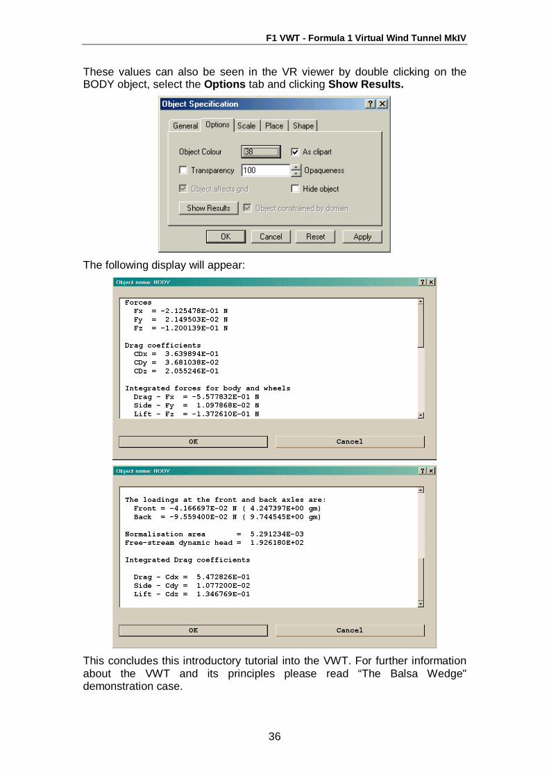
These values can also be seen in the VR viewer by double clicking on the BODY object, select the Options tab and clicking Show Results.
The following display will appear:
This concludes this introductory tutorial into the VWT. For further information about the VWT and its principles please read “The Balsa Wedge" demonstration case.

F1 VWT - Formula 1 Virtual Wind Tunnel MkΙV
37
Virtual Wind Tunnel – Tutorial – R Class The steps to be followed are exactly the same as for the D-class: 1. Generate the car body shape, then export an STL file. In this example, the
STL file is called ‘R6 F1 Car Template.stl’. The F1 STL import software will assume that the largest dimension is along the length of the car body, and that the z axis points up. The units are assumed to be millimetres.
If you have trouble with generating this body shape, a copy of the R6 F1 Car Template.stl file can be found in \phoenics\d_intfac\d_cadpho\d_stl. Copy this file to \phoenics\d_priv1, and proceed with the tutorial.
2. Start F1 VWT, click on File, Start New case, and select R-Class. The R-class balsa blank will appear.
3. Click on ‘Menu’ located on the VR handset, and change the title of the
simulation to 'R-Class Tutorial'
4. Click on and select the 'geometry file' option (currently selected as 'balsa-r'). This will open up a dialog in which the STL geometry file should be selected.
5. Click on ; here the 'Running Speed' is set, but for the purposes of this tutorial it should be left at 18 m/s (default). This is equivalent to 59 ft/s in the FPS unit system, which can be chosen at any time.
6. Click on . This window gives you the option to select the grid (coarse, medium, fine or user) and the number of iterations. For this tutorial the following selections should be made:
• Number of Iterations = 300 (default = 100) • Grid = Coarse.
NOTE: It is important that the 'Restart from Previous Run' option is set to 'off' (default). This window also gives the user an option to switch to full PHOENICS, but this should only be attempted in the presence of a teacher.
7. Click on and then 'OK'. This will take you back to the main VR environment. The car shape should change to:
F1 VWT - Formula 1 Virtual Wind Tunnel MkΙV
38
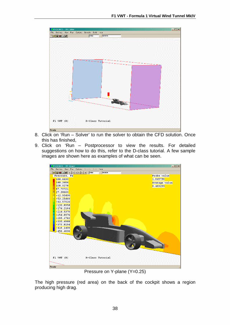
8. Click on ‘Run – Solver’ to run the solver to obtain the CFD solution. Once
this has finished, 9. Click on ‘Run – Postprocessor to view the results. For detailed
suggestions on how to do this, refer to the D-class tutorial. A few sample images are shown here as examples of what can be seen.
Pressure on Y-plane (Y=0.25)
The high pressure (red area) on the back of the cockpit shows a region producing high drag.

F1 VWT - Formula 1 Virtual Wind Tunnel MkΙV
39
Pressure surface contour
Velocity vectors on Y-plane (Y=0.25)
F1 VWT - Formula 1 Virtual Wind Tunnel MkΙV
40
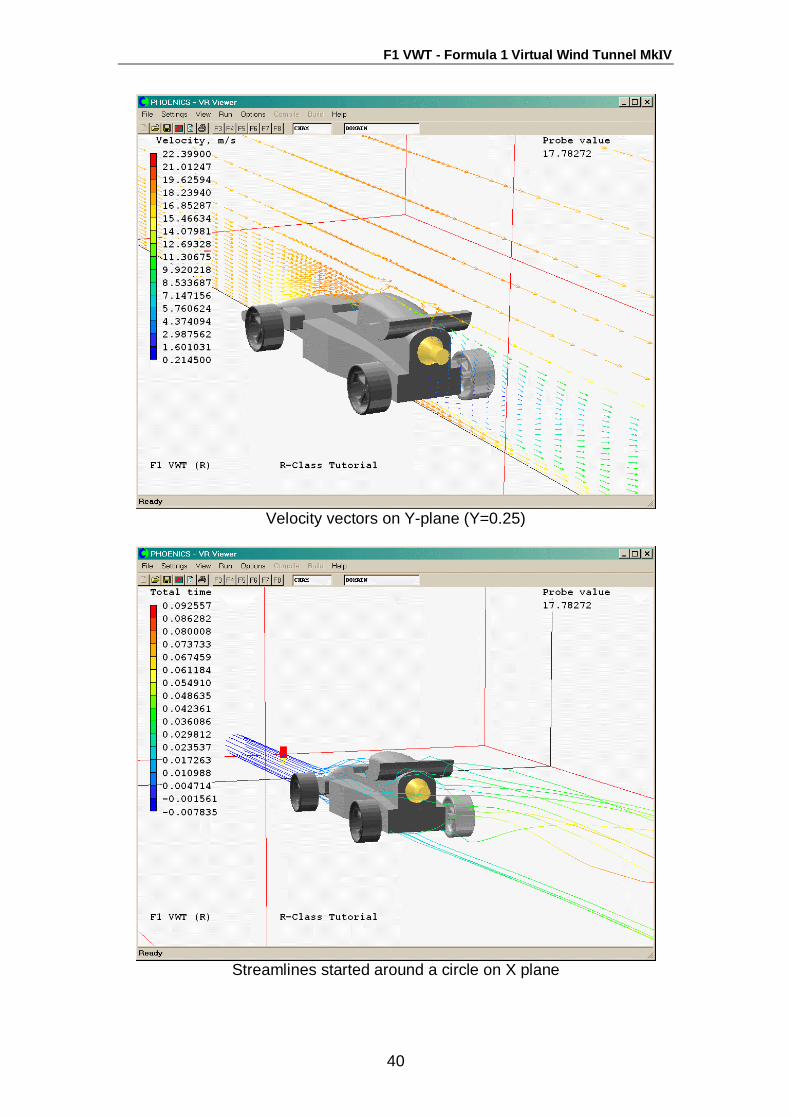
Velocity vectors on Y-plane (Y=0.25)
Streamlines started around a circle on X plane
F1 VWT - Formula 1 Virtual Wind Tunnel MkΙV
41
Demonstration Case - The Balsa Wedge 1. Introduction This demonstration case is designed to highlight further the versatility of the VWT. Although not an instructional example like the Grand Prix tutorial the balsa wood wedge simulation will show the following:
• The importance of grid refinement. • Aerodynamic improvements gained through modeling.
The structure of this demo will be to compare a 'coarse' and 'fine' meshed wedge example, followed by a comparison with the 'fine' Grand Prix case. This case was run with F1VWT MKll, so some of the screen images may no longer reflect the exact appearance of the current version.
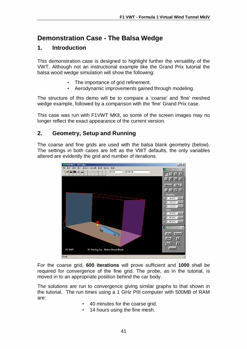
2. Geometry, Setup and Running The coarse and fine grids are used with the balsa blank geometry (below). The settings in both cases are left as the VWT defaults, the only variables altered are evidently the grid and number of iterations.
For the coarse grid, 600 iterations will prove sufficient and 1000 shall be required for convergence of the fine grid. The probe, as in the tutorial, is moved in to an appropriate position behind the car body. The solutions are run to convergence giving similar graphs to that shown in the tutorial. The run times using a 1 GHz PIII computer with 500MB of RAM are:
• 40 minutes for the coarse grid. • 14 hours using the fine mesh.
F1 VWT - Formula 1 Virtual Wind Tunnel MkΙV
42
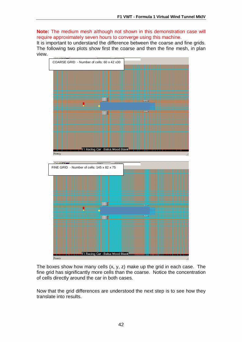
Note: The medium mesh although not shown in this demonstration case will require approximately seven hours to converge using this machine. It is important to understand the difference between the coarse and fine grids. The following two plots show first the coarse and then the fine mesh, in plan view.
The boxes show how many cells (x, y, z) make up the grid in each case. The fine grid has significantly more cells than the coarse. Notice the concentration of cells directly around the car in both cases. Now that the grid differences are understood the next step is to see how they translate into results.
COARSE GRID - Number of cells: 60 x 42 x30
FINE GRID - Number of cells: 145 x 82 x 75
F1 VWT - Formula 1 Virtual Wind Tunnel MkΙV
43
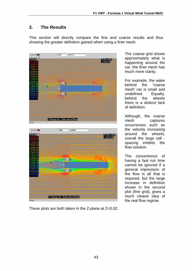
3. The Results This section will directly compare the fine and coarse results and thus showing the greater definition gained when using a finer mesh.
These plots are both taken in the Z-plane at Z=0.02.
The coarse grid shows approximately what is happening around the car, the finer mesh has much more clarity. For example, the wake behind the 'coarse mesh' car is small and undefined. Equally, behind the wheels there is a distinct lack of definition. Although, the coarse mesh captures occurrences such as the velocity increasing around the wheels, overall the large cell -spacing inhibits the flow solution. The convenience of having a fast run time cannot be ignored if a general impression of the flow is all that is required, but the largeincrease in definition shown in the second plot (fine grid), gives a much clearer idea of the real flow regime.
F1 VWT - Formula 1 Virtual Wind Tunnel MkΙV
44
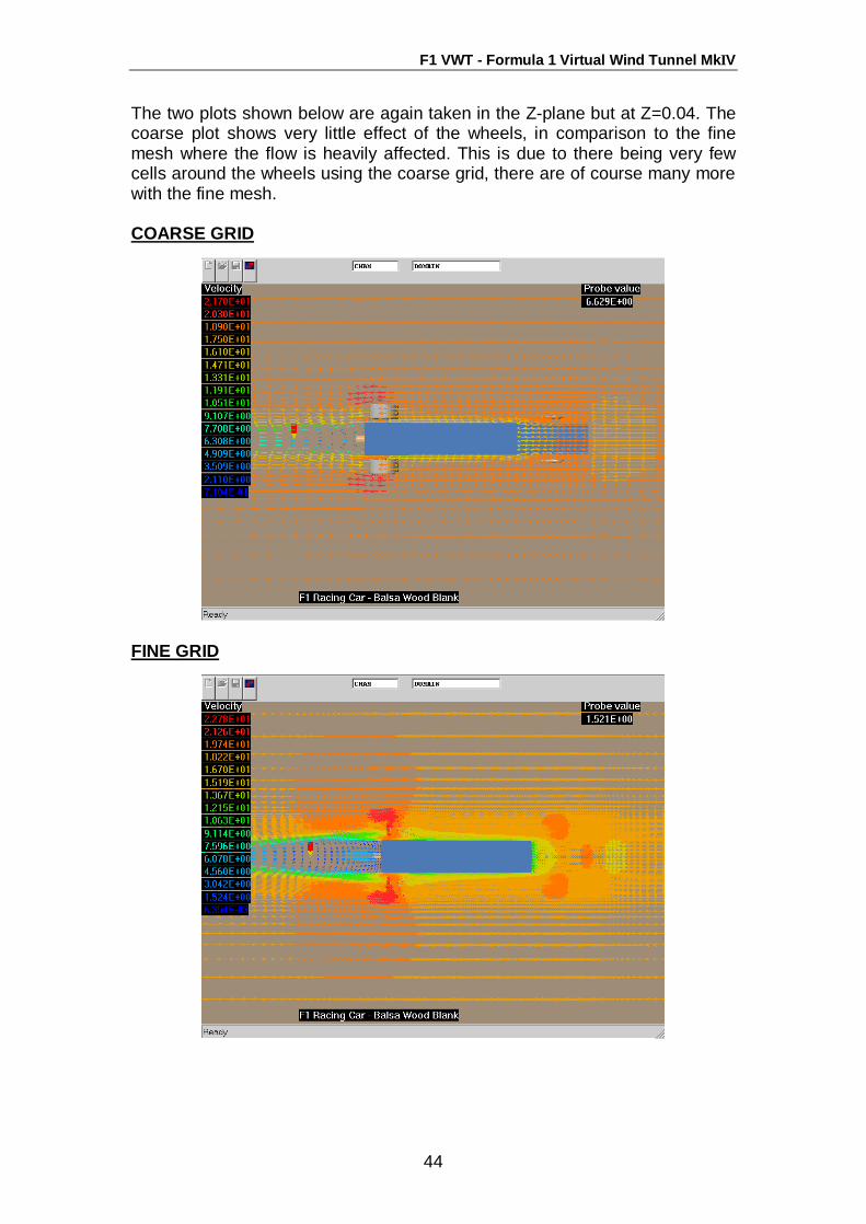
The two plots shown below are again taken in the Z-plane but at Z=0.04. The coarse plot shows very little effect of the wheels, in comparison to the fine mesh where the flow is heavily affected. This is due to there being very few cells around the wheels using the coarse grid, there are of course many more with the fine mesh. COARSE GRID
FINE GRID
F1 VWT - Formula 1 Virtual Wind Tunnel MkΙV
45
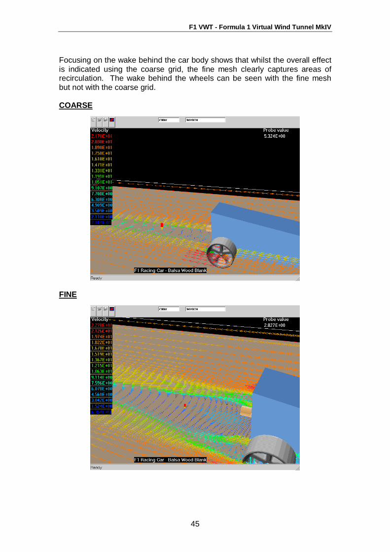
Focusing on the wake behind the car body shows that whilst the overall effect is indicated using the coarse grid, the fine mesh clearly captures areas of recirculation. The wake behind the wheels can be seen with the fine mesh but not with the coarse grid. COARSE
FINE

F1 VWT - Formula 1 Virtual Wind Tunnel MkΙV
46
These plots show the profile views of the car. An interesting point to note in the coarse grid plot is the step-effect along the top of the car, this is due to lack of cells and so the angular surface is not picked up accurately. The fine grid does not have this problem the increased number of cells has picked out the surface more accurately. (Note: For industry, "Body-Fitted" or "Adaptive Grid" meshes can also be used but these do not form part of the standard F1 VWT product.) Coarse
Fine
F1 VWT - Formula 1 Virtual Wind Tunnel MkΙV
47
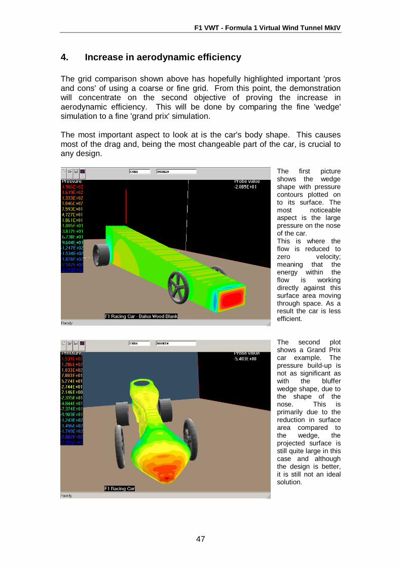
4. Increase in aerodynamic efficiency The grid comparison shown above has hopefully highlighted important 'pros and cons' of using a coarse or fine grid. From this point, the demonstration will concentrate on the second objective of proving the increase in aerodynamic efficiency. This will be done by comparing the fine 'wedge' simulation to a fine 'grand prix' simulation. The most important aspect to look at is the car's body shape. This causes most of the drag and, being the most changeable part of the car, is crucial to any design.
The first picture shows the wedge shape with pressure contours plotted on to its surface. The most noticeable aspect is the large pressure on the nose of the car. This is where the flow is reduced to zero velocity; meaning that the energy within the flow is working directly against this surface area moving through space. As a result the car is less efficient.
The second plot shows a Grand Prix car example. The pressure build-up is not as significant as with the bluffer wedge shape, due to the shape of the nose. This is primarily due to the reduction in surface area compared to the wedge, the projected surface is still quite large in this case and although the design is better, it is still not an ideal solution.
F1 VWT - Formula 1 Virtual Wind Tunnel MkΙV
48
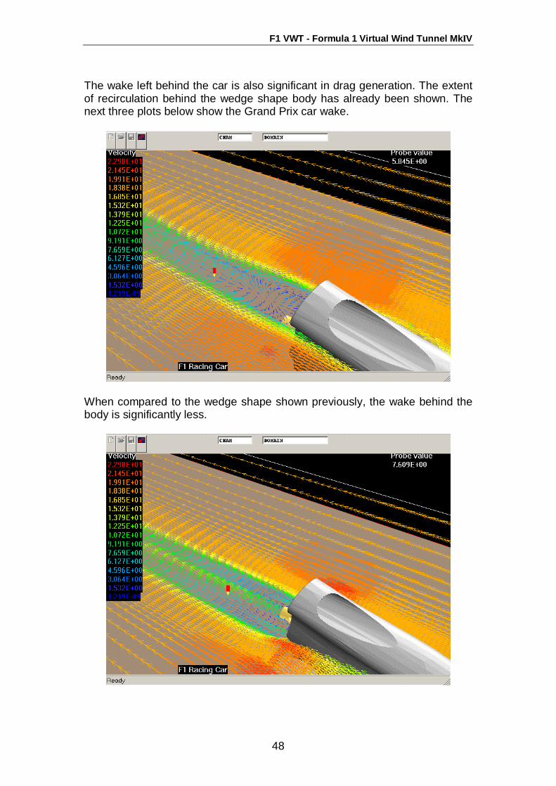
The wake left behind the car is also significant in drag generation. The extent of recirculation behind the wedge shape body has already been shown. The next three plots below show the Grand Prix car wake.
When compared to the wedge shape shown previously, the wake behind the body is significantly less.
F1 VWT - Formula 1 Virtual Wind Tunnel MkΙV
49
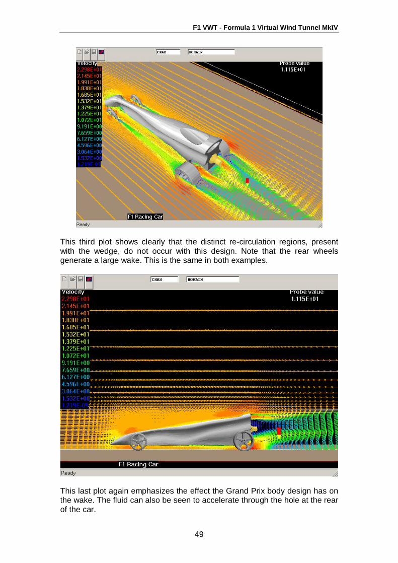
This third plot shows clearly that the distinct re-circulation regions, present with the wedge, do not occur with this design. Note that the rear wheels generate a large wake. This is the same in both examples.
This last plot again emphasizes the effect the Grand Prix body design has on the wake. The fluid can also be seen to accelerate through the hole at the rear of the car.
F1 VWT - Formula 1 Virtual Wind Tunnel MkΙV
50
5. The drag forces Another aspect of the VWT (as explained in the tutorial) is extracting the drag force data stored in the *.res file. The table below shows the comparison between the wedge and Grand Prix bodies. Balsa Wedge (body only) Grand Prix (body only)
Fx -2.709499E-01 N Fx -2.465826E-01 N Fy 1.458093E-03 N Fy -8.874801E-03 N Fz -2.537223E-02 N Fz -1.040585E-01 N CDx 4.925315E-01 CDx 3.972756E-01 CDy 5.735270E-04 CDy 3.348176E-03 CDz 1.045421E-02 CDz 3.885528E-02 The values for Fx (highlighted in red) are lower for the Grand Prix car, this is as expected due to its more aerodynamic shape. In conjunction with this the co-efficient of drag in x (CDx) (highlighted in blue) is significantly higher for the wedge shape. The final point to mention is the CD and forces in the Z direction. They will effectively represent down force generated by the car. These values are larger for the Grand Prix car. Within the results file is the same data for each object in the domain. The following table shows the drag components generated by the back wheels. Wedge (R-wheel only) Grand Prix (R-wheel only) Fx -1.442101E-01 N Fx -1.234675E-01 N Fy -6.596514E-03 N Fy 7.090292E-04 N Fz 8.877212E-02 N Fz 8.999211E-02 N CDx 4.248290E-01 CDx 3.637232E-01 CDy 4.919665E-02 CDy 5.287906E-03 CDz 2.625875E-01 CDz 2.661964E-01 As is expected the difference in CD and F for the same wheel on the two models is slight, with the only difference coming in the y direction but this can be attributed to the different body designs. From this data it is evident that the wheel adds significantly to the drag of the car, particularly when looking at the values of CDx and Fx.
This concludes this demonstration of the VWT. Further information can be gained by reading the "Jaguar F1 Car" demonstration case.
F1 VWT - Formula 1 Virtual Wind Tunnel MkΙV
51
Demonstration Case – Jaguar F1 Car 1. Introduction The simulation of the Jaguar F1 car was performed using the F1VWTMKll, so some of the screen images may not exactly reflect the appearance of the current version. The following document outlines the setup and results gained from the computation.
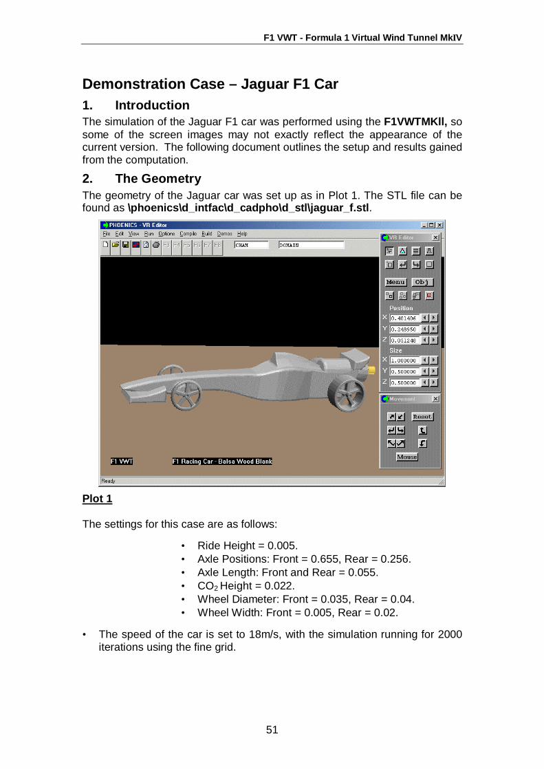
2. The Geometry The geometry of the Jaguar car was set up as in Plot 1. The STL file can be found as \phoenics\d_intfac\d_cadpho\d_stl\jaguar_f.stl.
Plot 1 The settings for this case are as follows:
• Ride Height = 0.005. • Axle Positions: Front = 0.655, Rear = 0.256. • Axle Length: Front and Rear = 0.055. • CO2 Height = 0.022. • Wheel Diameter: Front = 0.035, Rear = 0.04. • Wheel Width: Front = 0.005, Rear = 0.02.
• The speed of the car is set to 18m/s, with the simulation running for 2000 iterations using the fine grid.
F1 VWT - Formula 1 Virtual Wind Tunnel MkΙV
52
Note: 2000 iterations are enough to achieve a reasonable level of convergence; this should take approximately 35 hours using a PIII computer with 500MB of RAM.
F1 VWT - Formula 1 Virtual Wind Tunnel MkΙV
53
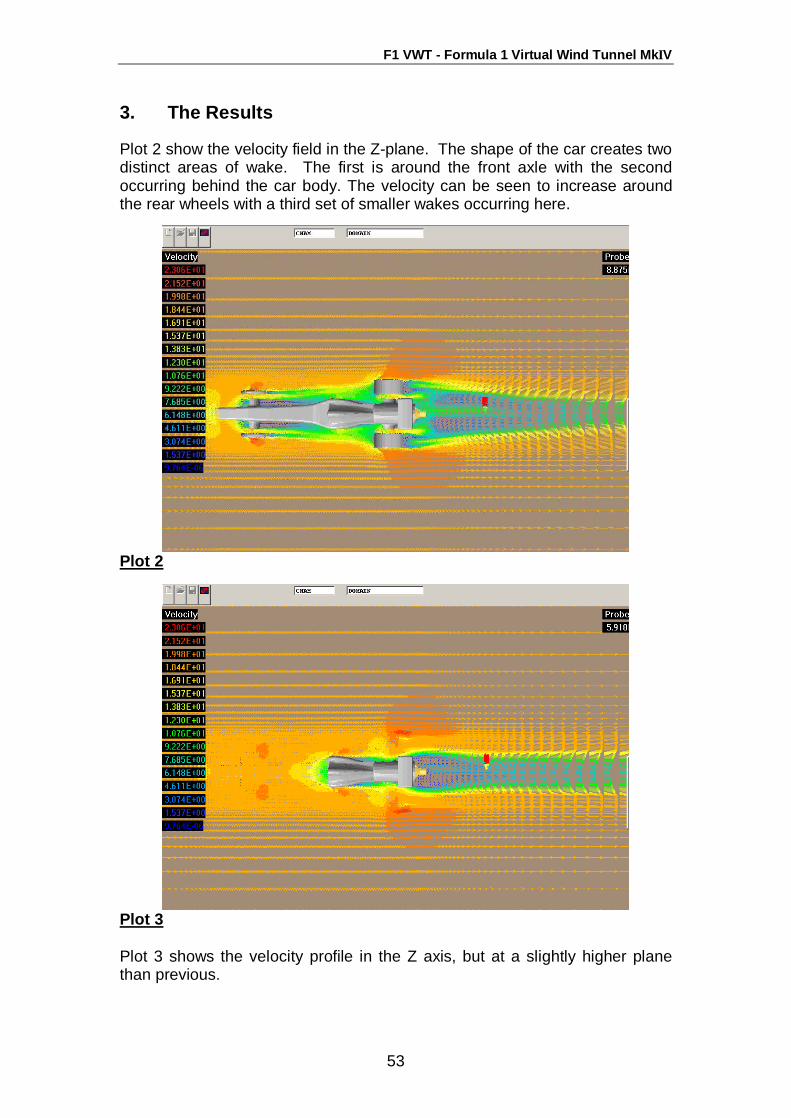
3. The Results Plot 2 show the velocity field in the Z-plane. The shape of the car creates two distinct areas of wake. The first is around the front axle with the second occurring behind the car body. The velocity can be seen to increase around the rear wheels with a third set of smaller wakes occurring here.
Plot 2
Plot 3 Plot 3 shows the velocity profile in the Z axis, but at a slightly higher plane than previous.
F1 VWT - Formula 1 Virtual Wind Tunnel MkΙV
54
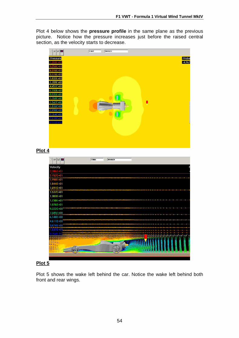
Plot 4 below shows the pressure profile in the same plane as the previous picture. Notice how the pressure increases just before the raised central section, as the velocity starts to decrease.
Plot 4
Plot 5 Plot 5 shows the wake left behind the car. Notice the wake left behind both front and rear wings.
F1 VWT - Formula 1 Virtual Wind Tunnel MkΙV
55
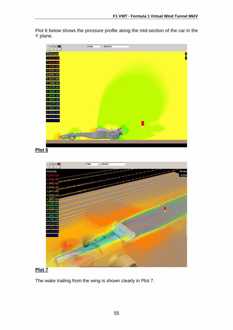
Plot 6 below shows the pressure profile along the mid-section of the car in the Y plane.
Plot 6
Plot 7 The wake trailing from the wing is shown clearly in Plot 7.
F1 VWT - Formula 1 Virtual Wind Tunnel MkΙV
56
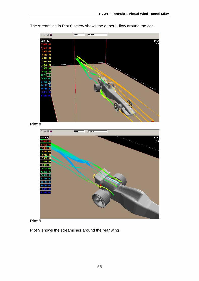
The streamline in Plot 8 below shows the general flow around the car.
Plot 8
Plot 9 Plot 9 shows the streamlines around the rear wing.
F1 VWT - Formula 1 Virtual Wind Tunnel MkΙV
57
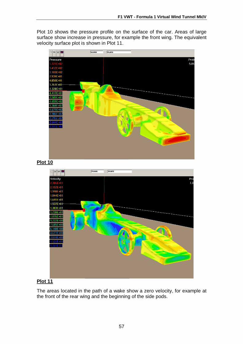
Plot 10 shows the pressure profile on the surface of the car. Areas of large surface show increase in pressure, for example the front wing. The equivalent velocity surface plot is shown in Plot 11.
Plot 10
Plot 11 The areas located in the path of a wake show a zero velocity, for example at the front of the rear wing and the beginning of the side pods.
F1 VWT - Formula 1 Virtual Wind Tunnel MkΙV
58
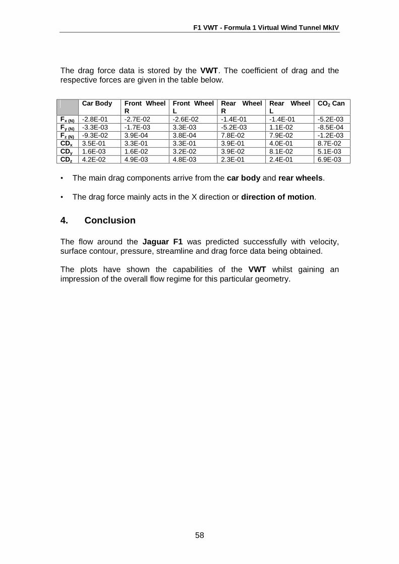
The drag force data is stored by the VWT. The coefficient of drag and the respective forces are given in the table below.
• The main drag components arrive from the car body and rear wheels. • The drag force mainly acts in the X direction or direction of motion.
4. Conclusion The flow around the Jaguar F1 was predicted successfully with velocity, surface contour, pressure, streamline and drag force data being obtained. The plots have shown the capabilities of the VWT whilst gaining an impression of the overall flow regime for this particular geometry.
Car Body Front Wheel R
Front Wheel L
Rear Wheel R
Rear Wheel L
CO2 Can
Fx (N) -2.8E-01 -2.7E-02 -2.6E-02 -1.4E-01 -1.4E-01 -5.2E-03 Fy (N) -3.3E-03 -1.7E-03 3.3E-03 -5.2E-03 1.1E-02 -8.5E-04 Fz (N) -9.3E-02 3.9E-04 3.8E-04 7.8E-02 7.9E-02 -1.2E-03 CDx 3.5E-01 3.3E-01 3.3E-01 3.9E-01 4.0E-01 8.7E-02 CDy 1.6E-03 1.6E-02 3.2E-02 3.9E-02 8.1E-02 5.1E-03 CDz 4.2E-02 4.9E-03 4.8E-03 2.3E-01 2.4E-01 6.9E-03