F-testtwo-sample t-test

Cochran-test

Variance analysis (ANOVA)

STATISSTATISTICSTICS

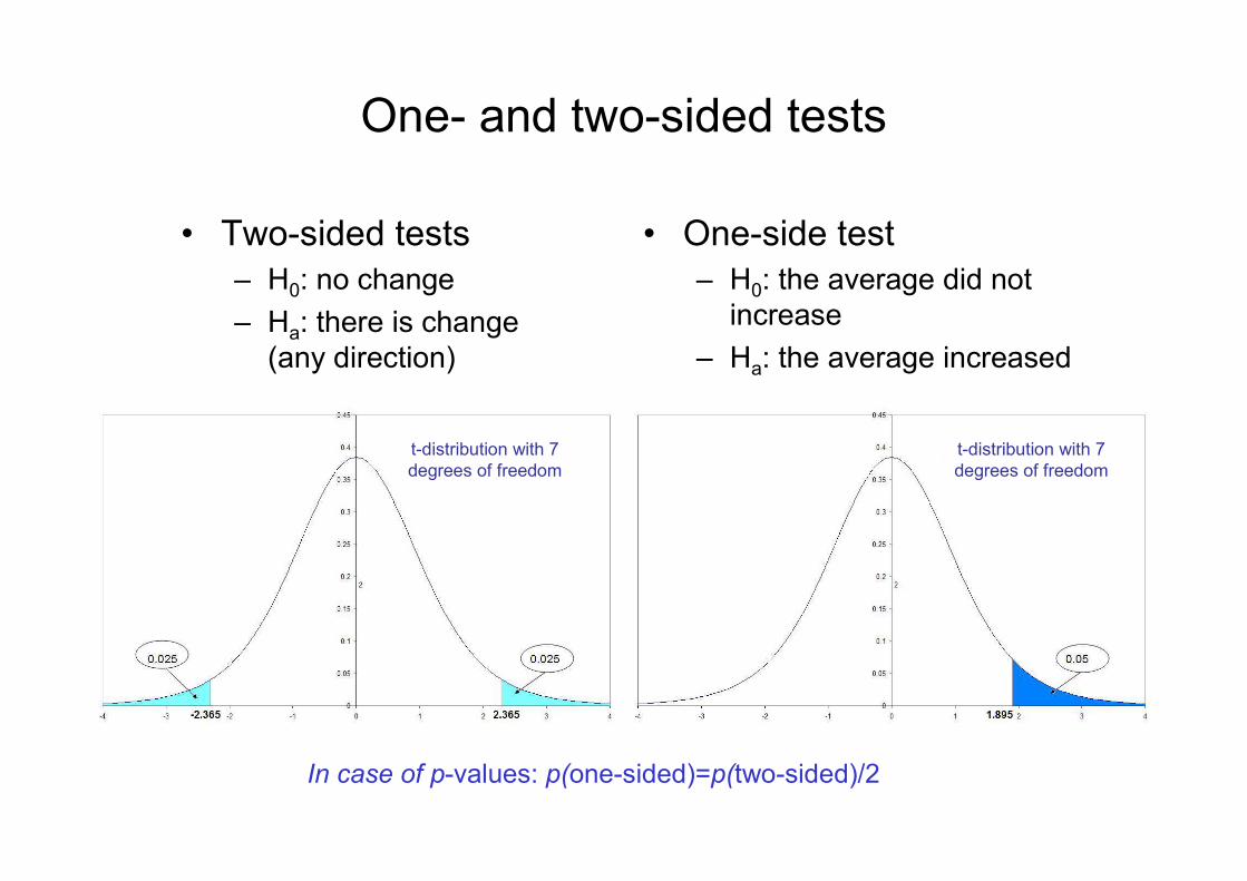
One- and two-sided tests

• Two-sided tests

– H0: no change

– Ha: there is change

(any direction)

• One-side test

– H0: the average did not

increase

– Ha: the average increased

In case of p-values: p(one-sided)=p(two-sided)/2

t-distribution with 7

degrees of freedom

t-distribution with 7

degrees of freedom

Interpretation of the significance

• Significant difference: p<α , p<0.05. It is stated that the compared populations are different. The probability errorof the decision is small (maximum α − this is the error of the first kind or Type I error).

• Non-significant difference: p>α , p>0.05. In this case, all you can say is that there is not sufficient information to detect the difference. Maybe– actually there is no difference;

– there is a difference, however only a few number of elementswere available;

– there was a standard deviation;

– it was wrong of the test method;

– 1

• Statistical significance should always be thought through whether for example it is significant in agricultural point of view;

• When providing statistical significance, indication of the p-value is also advisable;

FF--test for test for detectingdetecting identityidentity of of variancesvariances ofof twotwo

normallynormally distributeddistributed random random variablesvariables

� Our hypothesis for the identity of the variances of two independent

random variables of normal distribution with unknown expectation and

variance is checked by the so-called F-test.

� H0:

� H1:

� The test is always carried out as a one-sided test (it could be carried out

otherwise as well)

� Test statistics: , where

� If H0 fulfils, then Fsz is of F-distribution with degrees of freedom n1-1, n2-1

� Decision principle: for Fsz ≤ Fα 0-hypothesis is accepted, otherwise not.

22

21 σ=σ

22

21 σ>σ

22

*

21

*

szs

sF =

numerator: DF1 = n1 -1 denominator: DF2 = n2 -1

22

21

∗∗ > ss

ToTo be be peformedpeformed beforebefore tt--testtest!!

.

Two-sample t-test

( ) ( )2

11

21

222

211

21

21

21

−+

−+−⋅

+

−

nn

snsn

nn

nn

YY

2

22

1

21

21

n

s

n

s

YY

+

−

The test statistics received is of t-distribution with degrees of freedom n1 + n2 - 2

If the samples are independent,

normally distributed and their

standard deviations do not differ

significantly, they be seen as two

parts of a single sample.

Conditions of the t-test:

• For one-sample t-test:

• the random variable is normally distributed;

• the sample elements are independent;

• For two-sample t-test, in addition:

• standard deviations of the same two random variablesare identical;

Table of the t-distribution

and the test statistics of the

one-sample t-test

degree of

freedom critical values belongong to p

FF--test for test for detectingdetecting identityidentity of of variancesvariances ofof twotwo normallynormally distributeddistributed random random variablesvariables

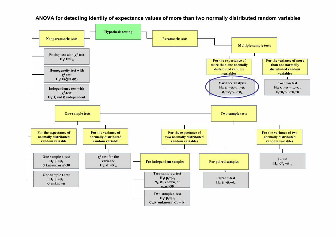
Hypothesis testing

Nonparametric tests Parametric tests

One-sample tests Two-sample tests

Multiple-sample tests

For the expectance of

normally distributed

random variable

For the variance of

normally distributed

random variable

One-sample z-test

H0: µ=µ0

σ known, or n>30

One-sample t-test

H0: µ=µ0

σ unknown

χ2-test for the

variance

H0: σ2=σ2

0

For the expectance of

two normally distributed

random variables

For the variance of two

normally distributed

random variables

Two-sample z-test

H0: µ1=µ2

σ1, σ2 known, or

n1,n2>30

Two-sample t-test

H0: µ1=µ2

σ1,σ2 unknown, σ1 = σ2

For independent samples For paired samples

Paired t-test

H0: µ1-µ2=d0

F-test

H0: σ21 =σ2

2

For the expectance of

more than one normally

distributed random

variables

For the variance of more

than one normally

distributed random

variables

Fitting test with χ2-test

H0: F=F0

Homogeneity test with

χ2-test

H0: F(ξ)=G(η)

Independence test with

χ2-test

H0: ξ and η independent

Variance analysis

H0: µ1=µ2=…=µn

σ1=σ2=…=σn

Cochran test

H0: σ1=σ2=…=σr

n1=n2=…=nr=n

TaskTask ((FF--test)test)

CO emissions of cigarettes from two different brands were

tested. The data were as follows. May we assume that the

standard deviation of the CO emission of the two brands are

the same?

„A” „B”

n 11 10

Mean 16,4 mg 15,6 mg

s* 1,2 mg 1,1 mg

SolutionSolution of of thethe tasktask ((FF--test)test)

H0: σ1 = σ 2

H1: σ1 > σ2

α = 0,05, DF1 = 10, DF2 = 9

F0,05 = 3,13

19,11,1

2,12

2

==szF

� Since Fsz occurs in the acceptance range, there is no reason to reject H0 in the 5% significance level.

Table of F-testCritical values of F-test at the 95% probability level

CochraCochran test for n test for detectingdetecting identityidentity of of variancesvariances ofof more more thanthan

twotwo normallynormally distributeddistributed random random variablesvariables

� Let r normally distributed random variables are given

� H0: σ1= σ2=…= σr

� H1: standard deviation of the variable having the maximum standard deviation, significantly differs from those of the others

� Cochran test can be applied if the element numbers of the random variables (n) are the same.

� Corrected empirical variance of the j-th sample:

� is the maximum corrected empirical variance among the values.

� Test statistics:

� Degree of freedom: DF = n - 1

� Knowing α, DF and r , ⇒ can be determined from the table of

Cochran test;

� Decision: if , then H0 is accepted, otherwise not.

2js∗

2maxs∗ 2

js∗

∑=

∗

∗

= r

1j

2j

2max

sz

s

sg

kritg

kritsz gg ≤

Hypothesis testing

Nonparametric tests Parametric tests

One-sample tests Two-sample tests

Multiple-sample tests

For the expectance of

normally distributed

random variable

For the variance of

normally distributed

random variable

One-sample z-test

H0: µ=µ0

σ known, or n>30

One-sample t-test

H0: µ=µ0

σ unknown

χ2-test for the

variance

H0: σ2=σ2

0

For the expectance of

two normally distributed

random variables

For the variance of two

normally distributed

random variables

Two-sample z-test

H0: µ1=µ2

σ1, σ2 known, or

n1,n2>30

Two-sample t-test

H0: µ1=µ2

σ1,σ2 unknown, σ1 = σ2

For independent samples For paired samples

Paired t-test

H0: µ1-µ2=d0

F-test

H0: σ21 =σ2

2

For the expectance of

more than one normally

distributed random

variables

For the variance of more

than one normally

distributed random

variables

Fitting test with χ2-test

H0: F=F0

Homogeneity test with

χ2-test

H0: F(ξ)=G(η)

Independence test with

χ2-test

H0: ξ and η independent

Variance analysis

H0: µ1=µ2=…=µn

σ1=σ2=…=σn

Cochran test

H0: σ1=σ2=…=σr

n1=n2=…=nr=n

Cochran test for detecting identity of variances of more than two normally distributed random variables

TaskTask ((CochranCochran test)*test)*

* Source: Kövesi J.: Kvantitatív módszerek, Oktatási segédanyag, BME MBA Mérnököknek program. (Quantitative methods, Educational aid, BME MBA for Engineers programme.) Budapest, 1998

� Műselyem For silk tensile strength testing of 20 pieces (r = 20), 10-item data for each r (n = 10), the following corrected empirical standard deviations were calculated for the tensile strength (see the table below). Is itpresumable that there is no significant difference between standard deviations of the random variables studied, if the level of significance is 5% ?

SolutionSolution of of thethe tasktask ((CochranCochran--testtest))

n = 10

2r

*22

*21

*

2max

*

szs...ss

sg

+++=

183,07,330

5,60gsz ==

� H0: standard deviations are identical

� H1: the highest standard deviations significantly differs fromthe others

DF = n-1= 10-1=9

r = 20, α = 5%gkrit = 0,135

kritsz gg > ⇒ H0 is rejected, namely the highest standard deviationsignificantly differs from the others.

i si2

i si2

1 24,9 11 12,5

2 8,4 12 11,4

3 21,2 13 4,8

4 8,0 14 22,2

5 8,4 15 22,6

6 6,0 16 16,1

7 26,3 17 10,9

8 26,7 18 9,6

9 6,8 19 60,5

10 12,5 20 10,9

Cochran-test, critical values of Gkrit

at the 5% probability level

Column 1: number of degrees of freedom;

Heading: r = number of groups (samples);

Mixed relationships – repetition

Similarity with ANOVA

ij

Indications

full difference

internal difference

external difference

full variance

internal variance

external variance

Calculation of variance

Total sum of

squares

Internal sum of

squares

External sum of

squares

ij

Relationships

full difference internal difference external difference

full variance internal variance external variance

Total sum of

squares

Internal sum of

squares

External sum

of squares

jxj

σ

Example:

In a college, bachelor training occurs in 4 professions. The

time spent on the students' daily learning is as follows.

Profession

Human resources

Management

International management

Finance & accounting

Time spent on daily learning (hr)

Mean *St. deviation

*Standard deviation

Calculate and interpret them!

Students

(%)

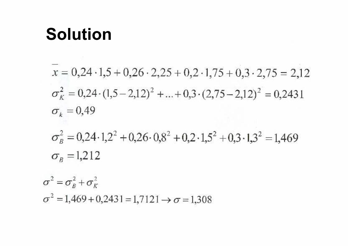
Solution

Indicators of mixed relationships

Quotient of standard deviations (square root of variance-ratio):shows that how strong is the relationship between the non-

quantitative (grouping) and quantitative criteria.

Variance-ratio: show that to what extent (in percentage) the

classification of a quality or areal criterion affects dispersion of a

quantitative criterion.

Interpretation of the indicators of themixed relationships

Stochastic relationships

Total independence, total lack of relationship

Function-like, deterministic relationship

Procedures based on ranking

(a type of non-parametric tests)

• What if the conditions of the t-test (normality, identity of variances) do not fulfil???– applying transformations (log, square root, arcsin, 1);

– non-parametric tests − procedures based on ranking;

• Non-parametric tests can be used if– the conditions of the parametric tests do not fulfil;

– we can not control (small sample size);

– we do not want to control;

– ordinal variables (how glad I am for spring??? − little, medium, verymuch);

• Only the magnitude of the data matters; it is unimportant how muchis one data bigger than the other;

• Calculation: based on ranking;

• BUT: not the same null hypothesis is tested as the parametric tests. So they cannot be regarded as non-parametric "equivalents " ofparametric tests;

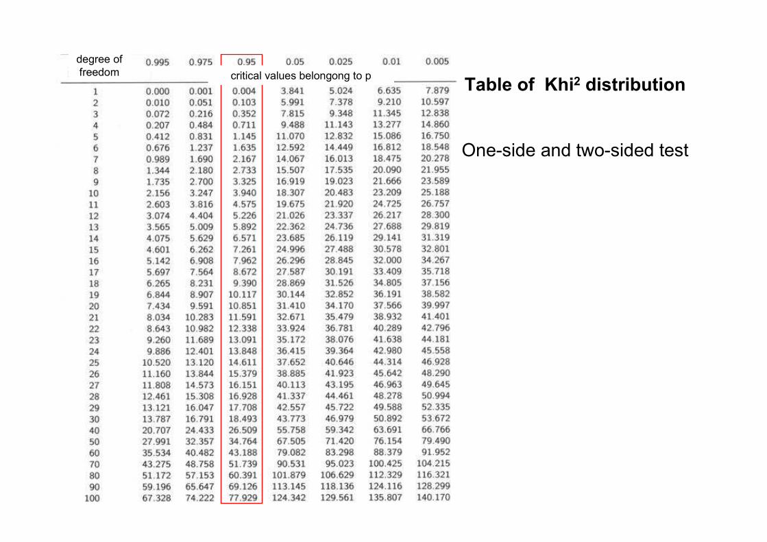
Table of Khi2 distribution

One-side and two-sided test

degree of

freedom critical values belongong to p

Studying more than two groups

One-way ANOVA

It’s base is a single F-test, which compares ”between groups” variance

(characterizing the differences of the means) to the ”within groups”

variance (characterizing random differences)

gfedcbatreatment type

basic data

variances

Why not perform pairwise comparisons?

• inefficient;

• it may distort our decisions, becausewhen making pairwise comparisons,random may also cause "significant" results;

if e.g. α=0,05, then on average, in every 20-th case, we're making a type I error, that is we reject a true 0-hypothesis;

In other words: we do not know which of the significant results are attributable to the random and which reflect a real difference.

• A lot of false comparison "inflates" the significance levels;

A kísérletenkénti első fajta hiba valószínűségének növekedése

0

0.1

0.2

0.3

0.4

0.5

0.6

0.7

0.8

0.9

1

0 10 20 30 40 50 60 70 80 90 100

Összehasonlítások száma

increase of type I error

probability per experiment

number of comparisons

err

or

of

pro

bab

ility

Repeated pairwise comparisons,

joint probabilities

Number of

indepedent

decisions

Nominal

significance level

Probability of

correct decision

Probability of

wrong decision

1 0.05 0.950 0.050

2 0.05 0.903 0.098

3 0.05 0.857 0.143

4 0.05 0.815 0.185

5 0.05 0.774 0.226

6 0.05 0.735 0,265

7 0.05 0.698 0.302

8 0.05 0.663 0.337

9 0.05 0.630 0.370

10 0.05 0.599 0.401

20 0.05 0.358 0.642

40 0.05 0.129 0.871

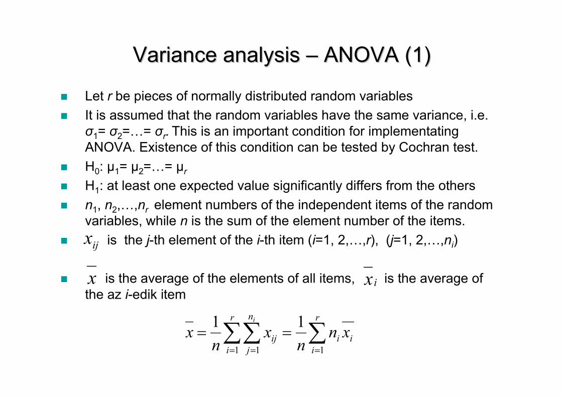
� Let r be pieces of normally distributed random variables

� It is assumed that the random variables have the same variance, i.e.

σ1= σ2=1= σr. This is an important condition for implementating

ANOVA. Existence of this condition can be tested by Cochran test.

� H0: µ1= µ2=1= µr

� H1: at least one expected value significantly differs from the others

� n1, n2,1,nr element numbers of the independent items of the random

variables, while n is the sum of the element number of the items.

� is the j-th element of the i-th item (i=1, 2,1,r), (j=1, 2,1,ni)

� is the average of the elements of all items, is the average of

the az i-edik item

∑∑∑== =

==r

i

ii

r

i

n

j

ij xnn

xn

xi

11 1

11

VarianceVariance analysisanalysis –– ANOVA (1)ANOVA (1)

ijx

x ix

� Let form the following statistics:

� SST=SSK+SSB;

� If H0 is true (and the identity of standard deviation fulfils), then

� SSB is of χ2-distribution with degree of freedom r-1 , while SSK is of

χ2-distribution with degree of freedom n-r ;

� SSK is independent from SSB; external variance and

internal variance are independent form each other,

their expectance value equal to each toher and to the unknown

variance of the population;

� To decide on variance equality, F-test is applied. If H0 fulfils, the test

staticstics is of F-distribution with degree of freedom r-1, n-r ;

( )∑=

−=r

1i

2

ii xxnSSK ( )∑∑= =

−=r

1i

n

1j

2

iij

i

xxSSB ( )∑∑= =

−=r

1i

n

1j

2

ij

i

xxSST

Csoportok közötti négyzetösszeg

Csoportokon belüli négyzetösszeg

Teljesnégyzetösszeg

12

−=

r

SSKsk

rn

SSBsb

−=2

22 / bksz ssF =

VarianceVariance analysisanalysis –– ANOVA (1)ANOVA (1)

External sum of squares

Internal sum of squares

Total sum of squares

VarianceVariance analysisanalysis –– ANOVA ANOVA tabletable

Name of sum of squares

Sum of squares

Degree of freedom

Assessment of st. dev.*

F-value p-value

Between groups

( )∑=

−r

i

ii xxn1

2 r-1 sk2 sk

2/sb2 p

Within groups

( )∑∑= =

−r

i

n

j

iij

i

xx1 1

2 n-r sb2 - -

Total ( )∑∑= =

−r

i

n

j

ij

i

xx1 1

n-1 - - -

� Two ways of decisions are possible:

� H0 is accepted, if Fsz ≤ Fkrit, otherwise H0 is rejected;

� H0 is accepted, if p>α , otherwise H0 is rejected;

� p-value is the maximum type I error probability (significance level) at

which the null hypothesis might be accepted;

� Calculations can be arranged into a so called ANOVA table

2

*standard deviation

Analysis of more than one groups consists

of two steps

• To determine whether there is a significant difference between the results of the set of groups;

• If it is so, then look for significant differences between the groups:– Difference may be not only in the form of difference between

groups;

Basic idea of the analysis: variance is

estimated in two ways in all samples

• The idea of ANOVA comes from R.A. Fisher, whoworked at an agricultural experimental station in England, between 1918-25.

• His ingenious Recognition: in experimentsperformed with several groups, null hypothesis H0

can also be examined so that the population varianceis estimated in two ways and the look whether thesethese estimates are in good agreement or not.

1. on the dispersions of within groups/samples we canconclude the variance of the population

2. on the dispersions of the groups/sample averages we can conclude the same variance .

The sum of squares can be divided

into additive elements

• Distance of the sub-sample elements from the highaverage of the whole sample is estimated by the sum of squares:

Σ (xhigh average– xi)² ;

• The sum of squares can be particioned by themethods of algebra (can be divided into parts additively)

• Each portion is decomposed so that they comply with the specific proportion of standard deviation

• The "internal" variance corresponds to the random, while of the variance "between the averages" meets the difference between the groups

One-way ANOVA

• Several independent samples are given

• Objective: comparison of averages

• Conditions: – The individuals get randomly to one or the other group, the

sample are independent (one individual cen get into one and only one group).

– The variable comprising the values to be compared iscontinuous.

– The samples come from normally distributed population.

– The populations from which the samples come, have equal variance.

• Null hypothesis:– The independent samples come from a population with the same

distribution, i.e.

the population averages are the same

Methodology

• ANOVA gets the total variance of the whole data set from two sources:– Between groups variance

– Within groups variance

• Starting null hypothesis: the population averages are the same;

The above assumption is equivalent to the following: between groups and within groups variances are the same in the population. By comparing thesetwo variances, one can conclude the identity of the averages.

• ‘New’ null hypothesis: between groups and within groups variances are the same in the population.

• Testing: estimation of the two variances are shown in the table below. The test statistic is the quotient of the two variances. Testing: F-test (one-sided).

• It gives a p-value: – if p>0.05, the we accept the identity of the averages (H0)

– if p<0.05, the there is at least one different in the averages

Calculations of analysis of variance used to be summarized in a table Reason of dispersion

Sum of squares Degress of freedom

Variance F-value

Between groups

2

1

)( xxnQ ii

t

i

k −= ∑=

t-1 1

2

−=

t

Qs k

k Fs

s

k

b

=2

2

Within groups 2

11

)( iij

n

j

t

i

b xxQi

−= ∑∑==

N-t tN

Qs b

b−

=2

Total 2

11

)( xxQ ij

n

j

t

i

i

−= ∑∑==

N-1

Illustration to the resolution

of the sum of squares

�Data

Average

High average

random component

grouping component

fixed value

Reasoning of ANOVA

• Samples were taken from normal distribution (eachsample has n element);

• Indipendent samples;

• Random samples (randomization);

• Null hypothesis: the samples come from one population;(v1=v2=v3=1=vn)

• Consequence of the null hypothesis : (s1

2=s22=s3

2=1=sn2)

• Two independent estimates are made from the samples to the standard deviation, more exactly variance of thepopulation (σ2);

• The quotient of the two estimates of variance follows F1,2

distribution (F1,2 = s12/s2

2);

(Analysis of Variance=ANOVA)

Reasoning of ANOVA (continued)

• If the samples come from one population (null-

hypothesis is true), then expectance value of the

distribuiton of F1,2 is: v(F1,2) = 1;

• If p<0,05 for F1,2 = 1, then the null-hypothesis is rejected;

• If the null-hypothesis is rejected, then we look for the

groups that do not come from one distribution.

• Pre-planned (a priori), or post (a posteriori) comparisons

are performed;

Distribution of the quotient of two variances;

Fisher–Snedecor distribution

Quotient of sum

of squares made

from normally

distributed

samples

F(m,n)=s1(m)2/s2(n)

2

Relationship between ANOVA and t-test

• In the denominator of the t-test formula the standard deviation of the mean is found;

• The numerator comprises a value corresponding to thestandard deviation: difference of means of two samples;

• This is none other than the difference of the two figures separately from their joint mean, divided by n-1, whichfor n = 2 equals one;

• In the numerator and denominator two estimates arefound for the same value, and the quotient of theirsquare is of F distribution;

Formula of the t-test, and its conversion

2

1

)(

2

21

22,1

2

221

22

21

2,1

21

21

−+

−

=

−+

−=

−+

nn

s

mm

t

nn

s

mmt

nn

If both sides of the formula is squared:

Then at the right hand side of the

formula we receive the quotient of

two variances, namely:

2,12

2 2121 −+−+ = nnnn Ft

v1

v2

v3

y

Group 1 Group 2 Group 3

The situation according to the null hypothesis

-3.5

0-1

.75

0.0

01

.75

3.5

0

-3.5

0-1

.75

0.0

01

.75

3.5

0

-3.5

0-1

.75

0.0

01

.75

3.5

0

Group 1 Group 2 Group 3

y

n

n

n

n

n

n

n

n

n

n

n

n

n

v1

v2

v3

The situation according to an alternative hypothesis

Reasoning following the

significant ANOVA

Two or more statistical decision in one analysis?

• What happens in type I error, if two completely independentexperiments are performed végzünk, when two independent samplesare compared.

• In this case, two independent hypothesis tests and two significance tests are performed, all at α=0,05 level. Since two independent investigations are concerned, the two significance testing can also be considered independent.

• If both null-hypothesis are valid, then the probability that at least, one of the null hypotheses is (incorrectly) rejected:

– Let P(s1)=0.05 is the above probability for the first test and P(s2)=0.05 the second aboveprobability.The probability of the joint occurrenc eof the two events P(s1)*P(s2), i.e., 0.05*0.05=0.0025

• The three possible events: s1 occurs alone, s2 occurs alone, whiles1 and s2 occur together.

• In the case of two independent experiments, the probability that at least in one of them the null hypothesis is (incorrectly) rejected:

p= 0.05+0.05-0.0025= 0.0975, which is significantly higher than 0.05 accepted for a single significance test.

• And if the experiments and comparisons are not independent?

Repeted pairwise comparisons,

joint probabilities

Number of

independent

decisions

Nominal

significance

level

Probability of

correct decision

Probability of

wrong decision

1 0.05 0.950 0.050

2 0.05 0.903 0.098

3 0.05 0.857 0.143

4 0.05 0.815 0.185

5 0.05 0.774 0.226

6 0.05 0.735 0.265

7 0.05 0.698 0.302

8 0.05 0.663 0.337

9 0.05 0.630 0.370

10 0.05 0.599 0.401

20 0.05 0.358 0.642

40 0.05 0.129 0.871

If there are many groups?

• If the above discussion is performed for k=10

independent tests then p=1-(1-0.05)10=0.4

• By increasing the number of independent analyses

we significantly increase the probability that such

effects exist, however in reality they do not exist

• Regarding every is possible significance tests,the tests are not independent, although thesamples were independent.

.

Hypothesis testing

Nonparametric tests Parametric tests

One-sample tests Two-sample tests

Multiple-sample tests

For the expectance of

normally distributed

random variable

For the variance of

normally distributed

random variable

One-sample z-test

H0: µ=µ0

σ known, or n>30

One-sample t-test

H0: µ=µ0

σ unknown

χ2-test for the

variance

H0: σ2=σ2

0

For the expectance of

two normally distributed

random variables

For the variance of two

normally distributed

random variables

Two-sample z-test

H0: µ1=µ2

σ1, σ2 known, or

n1,n2>30

Two-sample t-test

H0: µ1=µ2

σ1,σ2 unknown, σ1 = σ2

For independent samples For paired samples

Paired t-test

H0: µ1-µ2=d0

F-test

H0: σ21 =σ2

2

For the expectance of

more than one normally

distributed random

variables

For the variance of more

than one normally

distributed random

variables

Fitting test with χ2-test

H0: F=F0

Homogeneity test with

χ2-test

H0: F(ξ)=G(η)

Independence test with

χ2-test

H0: ξ and η independent

Variance analysis

H0: µ1=µ2=…=µn

σ1=σ2=…=σn

Cochran test

H0: σ1=σ2=…=σr

n1=n2=…=nr=n

ANOVA for detecting identity of expectance values of more than two normally distributed random variables

TaskTask (ANOVA)*(ANOVA)*

* Source: Curwin, J., Slater, R.: Quantitative Methods for Business Decisions, Third Edition,

Chapman & Hall, London, 1991

� Egy At 3 shops of a retail chain it was examined whether the same

amount was paid for a purchase. Each store selected six random

amount paid [in dollars] (see the table below). Assuming that the

payments are normally distributed and the standard deviations equal:

is there a difference between the three shops?

1. bolt 2. bolt 3. bolt

12,05 15,17 9,48

23,94 18,52 6,92

14,63 19,57 10,47

25,78 21,4 7,63

17,52 13,59 11,90

18,45 20,57 5,92

� H0: expectance value of thepurchase is the same in the threeshops

� H1: expectance value of thepurchase is not the same in thethree shops

SolutionSolution of of thethe tasktask (ANOVA) (1)(ANOVA) (1)

Shop 1 Shop 2 Shop 3

12.05 15.17 9.48

23.94 18.52 6.92

14.63 19.57 10.47

25.78 21.4 7.63

17.52 13.59 11.90

18.45 20.57 5.92

mean: 18.73 18.14 8.72

High average: 15.195

SSK= 6*(18.73-15.195)2 + + … = 378.4

Corrected empirical standard deviation: 5.288 3.106 2.281

SSB = 5.2882 ⋅ 5 +

+ 3.1062 ⋅ 5 +

+ 2.2812 ⋅ 5 =

= 214.1

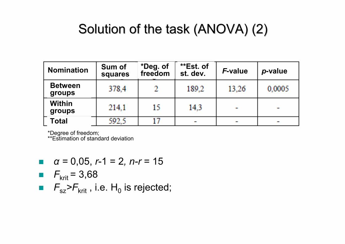
� α = 0,05, r-1 = 2, n-r = 15

� Fkrit = 3,68

� Fsz>Fkrit , i.e. H0 is rejected;

SolutionSolution of of thethe tasktask (ANOVA) (2)(ANOVA) (2)

Nomination

Betweengroups

Withingroups

Total

Sum of squares

*Deg. of freedom

**Est. of st. dev. F-value p-value

*Degree of freedom;**Estimation of standard deviation

Tasks: the name of the statistical method to be used, conditions of its carrying out,

and if further processes can also be used, then what is their ranking.

1. Some statistics of previous lottery drawings can be downloaded from the website

of the Szerencsejáték Rt. E.g. how many times the numbers have been pulled out

until now. How could be examined whether it has not been fraud; in other words,

whether certain numbers were pulled out in a significantly higher or smaller

frequency?

2. A company offers a new reagent claiming to more effectively increasing the

conductivity of a solution (it does not matter, why and how). Decide whether this

statement is true or not (method or methods)?

3. An entrepreneur sells an excipient, which (according to his statetment) increases

wheat yields. What method (or methods) can you decide that the statement is true?

4. We would like to compare dog breeds. Assume that there is a system of criteria,

according to which the animals examined can be graded from 0 to 4:

0 - mini, 1 - low, 2 - medium - large 3, 4 - huge.

Eight selected types of 366 dogs were analysed. What kind of statistical test can be

applied for detecting size difference among the types?

4.

Always look on the bright sideof things!

We finished for today, goodbye!

K قMNOPا RSTUPا VPإ TOXدا MZ[S TS\]د ^اT`abء!

让我们总是从光明的一面来看待事物吧！

今天的课程到此结束，谢谢！

ямарваа нэг зүйлийн гэгээлэгталыг нь үргэлж олж харцгаая

өнөөдөртөө ингээд дуусгацгаая, баяртай

abوم، وداhiذا اki alhkmlا !