extreme wind storms over europe: statistical analyses … · europe: statistical analyses of...
TRANSCRIPT

Arbeitsbericht MeteoSchweiz Nr. 216
Extreme wind storms over Europe: Statistical Analyses of ERA-40 P.M. Della-Marta, H. Mathis, C. Frei, M.A. Liniger, C. Appenzeller


Arbeitsbericht MeteoSchweiz Nr. 216
Extreme wind storms over Europe: Statistical Analyses of ERA-40 P.M. Della-Marta, H. Mathis, C. Frei, M.A. Liniger, C. Appenzeller
Bitte zitieren Sie diesen Arbeitsbericht folgendermassen Della-Marta, P.M., Mathis, H., Frei, C., Liniger, M.A., Appenzeller, C.: 2007, Extreme wind storms over Europe: Statistical Analyses of ERA-40, Arbeitsberichte der MeteoSchweiz, 216, 79pp.
Herausgeber Bundesamt für Meteorologie und Klimatologie, MeteoSchweiz, © 2007 MeteoSchweiz Krähbühlstrasse 58 CH-8044 Zürich T +41 44 256 91 11 www.meteoschweiz.ch
Weitere Standorte CH-8058 Zürich-Flughafen CH-6605 Locarno Monti CH-1211 Genève 2 CH-1530 Payerne


Abstract
Accurate assessment of the magnitude and frequency of extreme wind speed is of fundamentalimportance for many safety, engineering and �nancial applications. We utilise the spatial andtemporal consistency of the European Center for Medium Range Forecasts ERA-40 reanalysisdata to determine the frequency of extreme winds over the eastern North Atlantic and Europe.The analysis of extreme winds follows two di�erent view points: In a spatially distributed view,wind storm statistics are determined individually at each grid point over the domain, resultingin recurrence estimates of storms for each reanalysis grid point. In an integral, more general-ized view, the storm statistics are determined from extreme wind indices that summarize stormmagnitude and spatial extent. We investigated the quality of ERA-40 wind gust data, a param-eterised forecast �eld, and found the wind gust values over areas of complex orography to beunrealistic. This led to the need to mask these areas from further analysis. We also used the850hPa geostrophic wind speed which was found not to su�er from the same problems as windgust.
We applied classical peak over threshold (POT) extreme value analysis techniques to theextreme wind data. The POT series were �rst declustered using an automatic declustering tech-nique and then modelled using a Generalised Pareto Distribution (GPD) which was �tted usingmaximum likelihood estimation (MLE). The uncertainty in the return level and return period ofextreme winds was calculated using a number of di�erent methods including the standard deltamethod, bootstrap resampling and likelihood pro�le methods.
Extreme wind index (EWI) based return period estimates of prominent European stormsrange from approximately 0.3 to 100 years whereas grid point based return period estimatesrange from 0.3 to 1000+ years. The return period estimates derived from EWIs show a highdependence on the domain over which the indices are calculated, with generally higher returnsperiods for a given storm when considering land grid points compared to the calculations based onthe whole domain. EWI based return period estimates show greater dependence on the datasetused than on the EWI chosen. Generally higher return periods are derived from geostrophicwind than wind gust. An evaluation of the EWIs showed that they could explain between 0 and50% of the variability of local wind storm return periods obtained from the grid point analysis.The grid point analysis return period estimates are also dependent on the dataset chosen. Inparticular the advantages of complete coverage given by geostrophic wind speed over wind gustare partially o�set by aliasing of the wind extremity due to discrete analysis times, whereas windgust is an integrated quantity.

2

Contents
1 Introduction 11
1.1 Project background and literature overview . . . . . . . . . . . . . . . . . . . . . 11
2 Data and Extreme Wind Indices 15
2.1 PartnerRe high impact storm catalogue . . . . . . . . . . . . . . . . . . . . . . . 152.2 ERA-40 data . . . . . . . . . . . . . . . . . . . . . . . . . . . . . . . . . . . . . . 15
2.2.1 Data inhomogeneities . . . . . . . . . . . . . . . . . . . . . . . . . . . . . 162.3 Derived extreme wind indices . . . . . . . . . . . . . . . . . . . . . . . . . . . . . 18
2.3.1 Domain speci�cation . . . . . . . . . . . . . . . . . . . . . . . . . . . . . . 182.3.2 Extreme wind indices . . . . . . . . . . . . . . . . . . . . . . . . . . . . . 19
3 Extreme Value Analysis 21
3.1 The generalised Pareto distribution . . . . . . . . . . . . . . . . . . . . . . . . . . 213.2 Declustering and threshold selection . . . . . . . . . . . . . . . . . . . . . . . . . 223.3 Uncertainty calculations . . . . . . . . . . . . . . . . . . . . . . . . . . . . . . . . 27
4 The Return Period of Catalogue Wind Storms 33
4.1 The extreme wind distribution based on extreme wind indices . . . . . . . . . . . 334.2 The extreme wind distribution at each grid point . . . . . . . . . . . . . . . . . . 514.3 The return period of some prominent European wind storms . . . . . . . . . . . . 554.4 The evaluation of the extreme wind indices with grid point statistics . . . . . . . 594.5 Discussion of results . . . . . . . . . . . . . . . . . . . . . . . . . . . . . . . . . . 60
5 Conclusions and Recommendations for Further Research 63
5.1 Conclusions . . . . . . . . . . . . . . . . . . . . . . . . . . . . . . . . . . . . . . . 635.2 Recommendations for further research . . . . . . . . . . . . . . . . . . . . . . . . 64
Acknowledgements 67
Bibliography 69
3

4 CONTENTS
List of Tables
2.1 De�nition of sub domains, �� . . . . . . . . . . . . . . . . . . . . . . . . . . . . 19
4.1 The Spearman rank correlation between the Return Periods (RP) of cataloguestorms (96 storms) calculated from di�erent extreme wind indices (EWI, yellowshaded boxes, also described as inter -index ) and di�erent datasets (eitherWG72orGW72, red shaded boxes, also described as inter-dataset) over all grid points a),land only grid points b) and sea only grid points c). The labels �WG� and �GW�refer to wind gust and geostrophic wind respectively. The labelling of the EWIsis di�erent to that in the text, however the order of the indices is the same as theorder given in section 2.3. . . . . . . . . . . . . . . . . . . . . . . . . . . . . . . . 49
4.2 The RPs of some prominent wind storms in the storm catalogue during the 1989/90
and 1999/2000 extended winter season estimated using Q95, GW72 and �land. The last
column is an estimate of the range of RPs calculated over land only from the corresponding
grid point analyses shown in �gures 4.21 & 4.22. The columns denoted lower and upper
refer to the 95% con�dence interval boundaries respectively. Note that the date/time
�eld refers to the start date of the 72 hour integration period of the high resolution model
runs, see section 2.1 for more details. . . . . . . . . . . . . . . . . . . . . . . . . . . 564.3 As for table 4.2 but using the index Q95, WG72 and �land. Plots of grid point RPs are
not shown. . . . . . . . . . . . . . . . . . . . . . . . . . . . . . . . . . . . . . . . . 56
5

6 LIST OF TABLES

List of Figures
2.1 The roughness length, z0 (m) used in the ERA-40 reanalysis dataset (White, 2003;Uppala et al., 2005). . . . . . . . . . . . . . . . . . . . . . . . . . . . . . . . . . . 17
2.2 Areas (grid points shown in red) whereWG andWG72 from the ERA-40 reanalysiswere masked. Surface roughness, z0 (meters) greater than 3m a) and b) regionswhere the ERA-40 model orography is greater than 700m. . . . . . . . . . . . . . 17
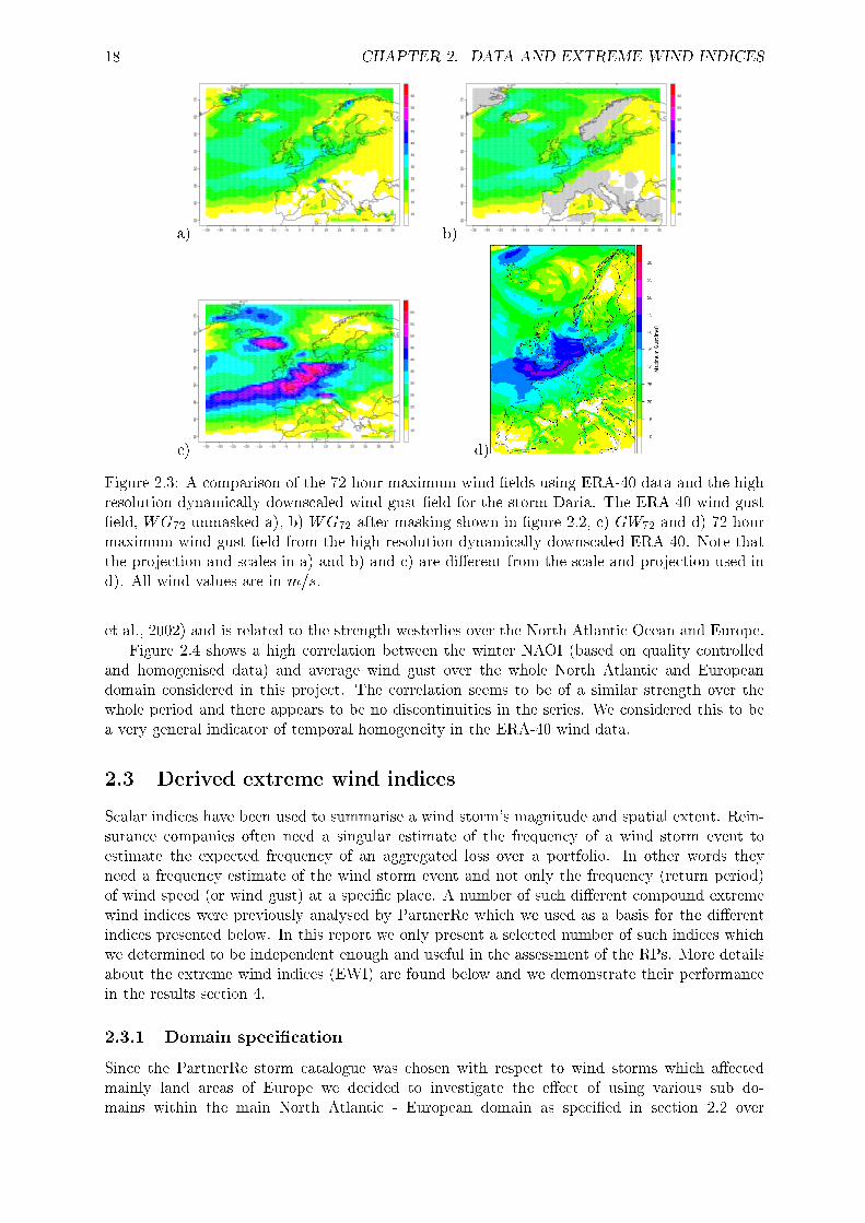
2.3 A comparison of the 72 hour maximum wind �elds using ERA-40 data and the highresolution dynamically downscaled wind gust �eld for the storm Daria. The ERA-40 wind gust �eld, WG72 unmasked a), b) WG72 after masking shown in �gure2.2, c) GW72 and d) 72 hour maximum wind gust �eld from the high resolutiondynamically downscaled ERA-40. Note that the projection and scales in a) andb) and c) are di�erent from the scale and projection used in d). All wind valuesare in m=s. . . . . . . . . . . . . . . . . . . . . . . . . . . . . . . . . . . . . . . . 18
2.4 Time series of mean WG over the domain (red line) using ERA-40 data and theNAOI index (black line) from 1958-2002. The NAOI used was from Hurrel et al.(2002). . . . . . . . . . . . . . . . . . . . . . . . . . . . . . . . . . . . . . . . . . 19
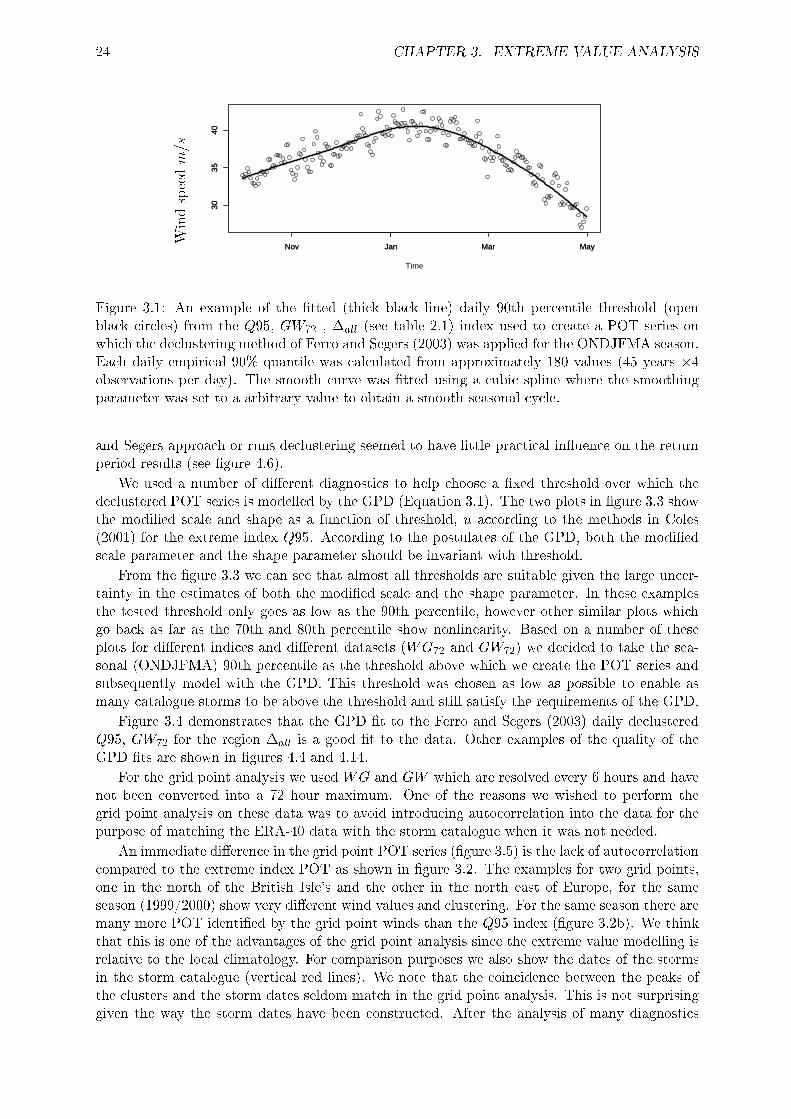
3.1 An example of the �tted (thick black line) daily 90th percentile threshold (openblack circles) from the Q95, GW72 , �all (see table 2.1) index used to create a POTseries on which the declustering method of Ferro and Segers (2003) was appliedfor the ONDJFMA season. Each daily empirical 90% quantile was calculatedfrom approximately 180 values (45 years �4 observations per day). The smoothcurve was �tted using a cubic spline where the smoothing parameter was set to aarbitrary value to obtain a smooth seasonal cycle. . . . . . . . . . . . . . . . . . 24
3.2 Examples of a daily declustered POT series using the approach of Ferro and Segers (2003)
for the extended winter season (ONDJFMA) of 1989/90 a) and b) 1999/2000. The thin
black line is the Q95 index calculated over the land only (�land) using GW72. The red
circles indicate values of the index which exceed the daily threshold (not shown). Blue
triangles show the maximum value of the index within each cluster. Membership of POTs
(red circles) to a particular cluster are denoted by colored bands on the top margin of
the plot. The solid and dashed grey lines show the daily 90th percentile and the seasonal
90th percentile respectively. The vertical red lines indicate the date of the storms in the
storm catalogue, with the names (from left to right, i.e. start of the season to the end
of the season) in a) unknown name, Daria, Herta, Nana, Vivian and Wiebke and in b)
Anatol, Lothar, Martin and Kerstin. . . . . . . . . . . . . . . . . . . . . . . . . . . . 25
7
8 LIST OF FIGURES
3.3 Modi�ed Scale, �� a) (see Coles, 2001) and the negative shape, ��, b) parameterdiagnostic plots for selecting the �xed threshold above which the declustered POTwill be modelled using the GPD. This example is based on the declustered POTQ95, GW72 for the region �all. The vertical black lines denote the 95% con�denceintervals calculated using the parametric resampling technique detailed in section3.3. The numbers aligned vertically in the top of the plot are the number of clustermaxima identi�ed by the declustering technique. The numbers in the header ofeach plot show the empirical quantile value at various cumulative probabilitiesfrom 0.9 to 0.99. . . . . . . . . . . . . . . . . . . . . . . . . . . . . . . . . . . . . 26
3.4 A quantile-quantile (qq) plot (m=s) of the �tted GPD to the declustered Q95,GW72 for the region �all. . . . . . . . . . . . . . . . . . . . . . . . . . . . . . . . 27
3.5 An example of a daily declustered POT series using the approach of Ferro and Segers
(2003) for the grid points 2.5� W, 57� N a) and b) 30� E, 67� N. The thin black line is
the GW during the extended winter season (ONDJFMA) of 1999/2000. The red circles
indicate values of the index which exceed the daily threshold (not shown). Blue triangles
show the maximum value of the wind within each cluster. Membership of POTs (red
circles) to a particular cluster are denoted by the colored bands on the top margin of the
plot. The solid and dashed grey lines show the daily 90th percentile and the seasonal
90th percentile respectively. The vertical red lines indicate the date of the storms in the
storm storm catalogue, with the names, Anatol, Lothar, Martin and Kerstin. . . . . . . 28
3.6 Modi�ed Scale, �� a) (see Coles (2001)) and the negative shape, ��, b) parameterdiagnostic plots for selecting the �xed threshold above which the declustered POTwill be modelled using the GPD. This example is based on the declustered POTGW for the grid point 2.5� W, 57� N. The vertical black lines denote the 95%con�dence intervals calculated using the parametric resampling technique detailedin section 3.3. The numbers aligned vertically in the top of the plot are thenumber of cluster maxima identi�ed by the declustering technique. The numbersin the header of each plot show the empirical quantile value at various cumulativeprobabilities from 0.95 to 0.99. . . . . . . . . . . . . . . . . . . . . . . . . . . . . 29
3.7 A comparison of the various methods used to calculate the uncertainty in theestimates of the RP (years) and RL (m=s). The example uses the GPD �t toQ95, GW72 and �all. Di�erent estimations of the 95% con�dence intervals: pro�lelog-likelihood (blue), delta method (green) and parametric resampling (red). . . . 31
4.1 The Return Period (RP, years) and Return Level (RL, m=s) of the GPD �t (blackline, equation 3.5) of the extreme wind index Q95, using geostrophic wind (GW72
) over the European land domain (�land). The black dots represent the maximaof the declustered POT series. Blue lines show the upper and lower bounds ofthe 95% con�dence interval of both RL and RP calculated using pro�le log like-lihood. The horizontal green and vertical red lines denote the RL and RP of thecatalogue storms respectively. The dashed grey line denotes the 90th percentilethreshold above which the declustered peaks were chosen. Note the log scale onthe horizontal axis. . . . . . . . . . . . . . . . . . . . . . . . . . . . . . . . . . . . 34
4.2 The RP and RL of the GPD �t to the �ve EWIs calculated over the whole domain.RL (m=s, vertical axis) versus RP (years, horizontal axis) with uncertainty (pro�lelog likelihood) estimates. Indices based on WG72 and �all�masked (left column)and indices based on GW72 and �all (right column). a) and b) �X, c) and d)Q95, e) and f) SQ95, g) and h) Sfq95, i) and j) Sfq95q99. Green and red linesindicate the RL and RP of the the 96 PartnerRe storms within the ONDJFMAseason. The dashed grey line denotes the 90th percentile threshold above whichthe declustered peaks were chosen. . . . . . . . . . . . . . . . . . . . . . . . . . . 36

LIST OF FIGURES 9
4.3 The RP and RL of the GPD �t to the �ve EWIs calculated over land. RL (m=s,vertical axis) versus RP (years, horizontal axis) with uncertainty (pro�le log like-lihood) estimates. Indices based on WG72 and �land�masked (left column) andindices based on W 850
72geo and �land (right column). a) and b) �X, c) and d) Q95,e) and f) SQ95, g) and h) Sfq95, i) and j) Sfq95q99. Green and red lines in-dicate the RL and RP of the the 96 PartnerRe storms within the ONDJFMAseason. The dashed grey line denotes the 90th percentile threshold above whichthe declustered peaks were chosen. . . . . . . . . . . . . . . . . . . . . . . . . . . 37
4.4 Quantile-quantile plots for the GPD �t to the �ve EWIs calculated over land. Em-pirical ( vertical axis) versus model (horizontal axis). Indices based on WG72 and�land�masked (left column) and indices based on GW72 and �land (right column).a) and b) �X, c) and d) Q95, e) and f) SQ95, g) and h) Sfq95, i) and j) Sfq95q99. 38
4.5 The RP and RL of the GPD �t to the �ve EWIs calculated over sea only. RL(m=s, vertical axis) vs. RP (years, horizontal axis) with uncertainty (pro�le loglikelihood) estimates. Indices based on WG72 and �sea�masked (left column) andindices based on GW72 and �sea (right column). a) and b) �X, c) and d) Q95, e)and f) SQ95, g) and h) Sfq95, i) and j) Sfq95q99. Green and red lines indicatethe RL and RP of the the 96 PartnerRe storms within the ONDJFMA season. Thedashed grey line denotes the 90th percentile threshold above which the declusteredpeaks were chosen. . . . . . . . . . . . . . . . . . . . . . . . . . . . . . . . . . . . 39
4.6 Comparison of the �tted GPD using runs declustering and the Ferro and Segers method.
Quantile-quantile plot of Q95, WG72, �land using runs declustering a) and Ferro and
Segers (2003) b). In c) a scatter plot of the RPs of catalogue storms comparing the two
methods. Note the logarithmic scale. 95% con�dence intervals for each of the RP are
denoted by orange (Ferro and Segers, 2003) and blue (runs declustering) whiskers on each
scatter plot point. Solid black line denotes the equal RP line. At the bottom of each
sub-�gure is the Spearman rank and Kendall's Tau correlation coe�cient. . . . . . . . . 40
4.7 A summary of the range of Return Periods (RP, years) of the catalogue stormsgiven by each of the �ve extreme wind indices (section 2.3) using wind gust (WG72
left, yellow boxplots) and geostrophic wind (GW72, right, red boxplots) over theEuropean land domain (�land and �land�masked respectively). The numbers onthe horizontal axis refer to the EWIs, �X, Q95, SQ95, Sfq95, and Sfq95q99,respectively. The solid black line of each boxplot represent the median, the in-terquartile range (coloured area), 1.5 times the interquartile range (dashed blackline) and the outliers (open circles). . . . . . . . . . . . . . . . . . . . . . . . . . 41
4.8 Comparison of Return Periods (RP, years) for the 96 PartnerRe wind storms calculated
using the extreme wind index (EWI, �X) based on wind gust (WG72, labelled as fg10
on the plot) and geostrophic wind speed (GW72, labelled as gws on the plot). Note the
logarithmic scale. 95% con�dence intervals for each of the RP are denoted by red (WG72)
and blue (GW72) whiskers on each scatter plot point. a) using domain �all�masked and
�all; b) using domain �land�masked and �land, c) using domain �land�masked and �sea
for WG72 and GW72 respectively. Solid black line denotes the equal RP line. At the
bottom of each sub-�gure is the Spearman rank and Kendall Tau correlation coe�cient. 43
4.9 As for �gure 4.8 but using Q95 . . . . . . . . . . . . . . . . . . . . . . . . . . . . 44
4.10 As for �gure 4.8 but using SQ95 . . . . . . . . . . . . . . . . . . . . . . . . . . . 45
4.11 As for �gure 4.8 but using Sfq95 . . . . . . . . . . . . . . . . . . . . . . . . . . . 46
4.12 As for �gure 4.8 but using Sfq95q99 . . . . . . . . . . . . . . . . . . . . . . . . . 47

10 LIST OF FIGURES
4.13 The e�ect of masking unrealistic wind gust grid points on return period estimates. Scatter
plot of RPs (years) for the 96 catalogue wind storms calculated using Q95, WG72 versus
the RPs calculated using Q95, GW72. a) using domain �land�masked and �land; b) using
domain �land�masked and �land�masked for WG72 and GW72 respectively and c) using
GW72 domain �land�masked and �land. Solid black line denotes the equal RP line. Note
the logarithmic scale. 95% con�dence intervals for each of the RP are denoted by red and
blue (green and orange) for WG72and GW72 in a) and b) and in c) the colours brown
and purple are used to denote the RP con�dence intervals of GW72 �land�masked and
�land respectively. At the bottom of each sub-�gure is the Spearman rank and Kendall
Tau correlation coe�cient. . . . . . . . . . . . . . . . . . . . . . . . . . . . . . . . . 504.14 The RL (m=s) and RP (years) of the GPD �t to the GW at two grid points in
the analysis domain, 2.5� E, 57� N a) and c) 30� W, 67� N. The correspondingquantile-quantile plots are shown in b) and d) respectively. . . . . . . . . . . . . . 51
4.15 Important parameters of the grid point EVA (section 3) based on GW . The gridpoint empirical 95% quantile threshold, u (m=s) a), the MLEs of the GPD �t(equations 3.1 and 3.5 ) for � (the average number of declustered exceedances ofthe 95% quantile threshold) b), � (the scale parameter of the GPD) c), � (theshape parameter of the GPD) d), and the extremal index, � (equation 3.8) e). . . 52
4.16 The RL of GW at each grid point (m=s) over the extended winter season (October- April), for RPs of 1 year a), 5 years b), 20 years c) and 50 years d). . . . . . . . 53
4.17 Scatter plot of RPs (years) for the 96 catalogue wind storms calculated using WG(labelled fg10 on the plot)versus the RPs calculated using, GW (labelled gws onthe plot) at various grid points, a) 3� W, 48� N, b) 5� W, 53� N and c) 25� E,55� N. Note the logarithmic scale. 95% con�dence intervals for each of the RP aredenoted by purple (WG) and light blue (GW ) whiskers on each scatter plot point.Solid black line denotes the equal RP line. At the bottom of each sub-�gure is theSpearman rank and Kendall Tau correlation coe�cient. . . . . . . . . . . . . . . . 54
4.18 The RP (years) for each grid point estimated from a) WG and b) GW for thestorm Anatol: 19891215 0600UTC. . . . . . . . . . . . . . . . . . . . . . . . . . . 55
4.19 The RP (years) for each grid point estimated from a) WG and b) GW for thestorm Herta: 19900201 0000UTC. . . . . . . . . . . . . . . . . . . . . . . . . . . . 55
4.20 The return period (RP, years) of geostrophic wind (GW ) for each grid pointestimated from for the storm Daria: 19900123 1200UTC b). In a) (c) is shownthe upper (lower) bound of the 95% con�dence interval of the RP (years). . . . . 57
4.21 The RP (years) for each grid point for each catalogue storm in the 1990/90 October- April extended winter season estimated from GW and using the EVA detailed insection 3. a) unknown name: 19891215 0600UTC, b) Daria: 19900123 1200UTC ,c) Herta: 19900201 0000UTC, d) Nana: 19900210 1800UTC, e) Vivian: 199002241200UTC, f) Wiebke: 19900226 0600UTC. The RP scale is in the top left of theplot. . . . . . . . . . . . . . . . . . . . . . . . . . . . . . . . . . . . . . . . . . . . 58
4.22 The RP (years) for each grid point for each catalogue storm in the 1999/2000 Octo-ber - April extended winter season estimated fromGW and using the EVA detailedin section 3. a) Anatol: 19991201 1200UTC, b) Lothar: 19991223 1800UTC , c)Martin: 19991225 1200UTC, d) Kerstin: 20000127 1800UTC. The RP scale is inthe top left of the plot. . . . . . . . . . . . . . . . . . . . . . . . . . . . . . . . . . 59
4.23 The Spearman rank correlation between the return periods of the 96 cataloguestorms based on Q95 of GW72 and the return period at each grid point based onGW , a) over �all , and b) �land. . . . . . . . . . . . . . . . . . . . . . . . . . . 60
4.24 The Spearman rank correlation between the return periods of the 96 cataloguestorms based on �X of GW72 and the return period at each grid point based onGW , a) over �all , and b) �land. . . . . . . . . . . . . . . . . . . . . . . . . . . 60

Chapter 1
Introduction
1.1 Project background and literature overview
Accurate knowledge of the frequency distribution of strong surface wind, in particular wind gusts,is of major relevance for insurance related risks in Europe. Reliable climatologies based on in-situwind observations are almost impossible to obtain as the observations are too coarse in spaceand/or short and inhomogeneous in time. There are several alternative data sources and analysistechniques that can be used in place of in-situ wind data, each with their own strengths andweaknesses. This study was in part motivated by the needs of the reinsurance industry. In orderto estimate the climate impacts of extreme wind events (or any other geophysical extreme event)both in the past and the future, we need an accurate estimate of the magnitude of the extremewind events as well as their frequency. We take an example from the reinsurance industry,who underwrite the risk of damage caused by strong wind events. A �rst impression of thevulnerability, or risk, comes from data gathered on the particular impact of interest, in thiscase high wind induced damage to property, or in monetary terms, loss. The estimates of lossare not representative of the meteorological hazard since loss is a�ected by many other factorswhich are non-stationary in time and space. To model loss, it is necessary to have an accurateknowledge of the meteorological hazard itself, including an estimate of the uncertainty. Withoutaccurate knowledge of the hazard risk the best estimate of uncertainty in the risk of loss is notknown. In order to obtain accurate information on the magnitude of surface wind during windstorm events the reinsurance company PartnerRe has obtained approximately 100 high resolutiondynamically downscaled wind storms from a previous project with MeteoSwiss (Schubiger et al.,2004; Turina et al., 2004). For each wind storm, a modi�ed version of the MeteoSwiss limited areaweather forecast model was run using ERA-40 boundary conditions. The high resolution windstorm simulations are ideally suited to the analysis of the local scale wind induced reinsurancelosses since they o�er a complete spatial coverage of the eastern North Atlantic and westernEurope. Another advantage of the high resolution simulations is that the surface wind speedsare similar in magnitude to in-situ measurements (Weisse et al., 2005; Leckebusch et al., 2006;Walser et al., 2006). Therefore, dynamical downscaling can provide more accurate estimates ofwind storm magnitude. However, with only a limited number of simulated events, which havebeen subjectively chosen, accurate determination of the frequency of such events is not possible.
The overall aim of this study is to characterise the climate of extreme winds over Europe andthe North Atlantic and to de�ne the return periods (frequency) of some prominent high impactwind storm events. Reinsurance companies often need a singular estimate of the frequency ofa wind storm event to estimate the expected frequency of an aggregated loss over a portfolio.Keeping this in mind, and given that the domain of interest is large in scale, we have chosen to usereanalysis data as the basis of this climatology since their is generally a lack of large scale, hightemporal and spatial resolution in-situ wind or derived wind datasets available to the climatecommunity for this type of analysis. Reanalysis datasets generated by data assimilation in state ofthe art global weather forecasting models provide a new source of information for meteorological
11

12 CHAPTER 1. INTRODUCTION
statistics (Uppala et al., 2005). Reanalyses provide the temporal extent and homogeneity forcomparisons in the frequency domain (e.g. Caires and Sterl, 2005), and the spatial coverage andphysical consistency for a continental-scale overview. The quality of reanalyses depends stronglyon the parameter, for example, temperature is well captured, even in mountainous areas (Kunzet al., 2007), other parameters like integrated water vapour (Morland et al., 2006) or precipitationmight be less realistic in absolute terms. In particular there can be serious biases in absolutewind values (Smits et al., 2005) and in some �elds obvious inhomogeneities (Bengtsson et al.,2004; Sterl, 2004; Smits et al., 2005).
Previous studies documenting the extreme wind climate of the North Atlantic and Europe usea number of di�erent data and methodologies depending on the aim of the study. Those aimedat characterising the absolute mean and extreme wind climate at a local level, with or withoutspecial attention to time trends have analysed in-situ wind data directly. These studies have hada focus on obtaining the most accurate estimate of return levels (RL), or absolute magnitude ofwind or wind gust (Dukes and Palutikof, 1995; Kristensen et al., 1999; Kasperski, 2002; Sacré,2002; Smits et al., 2005; Bouette et al., 2006; Graybeal, 2006; Walter et al., 2006). Usually, digitalaccess to daily or sub-daily wind measurements on a European scale more than 50 years in lengthpresent challenges to using this data (Alexander et al., 2005). Generally it is accepted that in-situwind data present some serious problems of data homogeneity (although methods exist to correctfor exposure, e.g. Verkaik, 2000) and so most studies aimed at determining long term trends andvariability have focused on either air pressure observations (Schinke, 1993; Kaas et al., 1996;Alexandersson et al., 1998, 2000; Carretero et al., 1998; Lamb, 1991; Barring and von Storch,2004; Alexander et al., 2005; Smits et al., 2005), derived wind from air pressure observations(Miller, 2003; Schmith et al., 1998), sea level datasets (e.g. Bijl et al., 1999), derived wind fromactive and passive microwave sensors aboard satellites (e.g. Monahan, 2006) or use of reanalysisdata (Pryor and Barthelmie, 2003; Smits et al., 2005; Weisse et al., 2005; Yan et al., 2002, 2006;Seierstad et al., 2007). A growing number of studies have used high resolution numerical modelsto downscale global reanalysis data in order to obtain an accurate estimate of wind magnitude(e.g. Turina et al., 2004; Schubiger et al., 2004; Leckebusch et al., 2006; Walser et al., 2006;Walter et al., 2006).
Climate change has promoted a wide study of the potential impacts of the enhanced green-house e�ect on the frequency, duration and intensity of wind storms in a future climate comparedto today. Held (1993) provides a good introduction into the response of large scale climate toglobal warming. In particular, with relation to mid-latitude �ow, the opposing e�ects betweenchanges in the lower tropospheric and mid-tropospheric temperature gradients and the role ofincreased moisture availability. Recent studies such as Knippertz et al. (2000); Leckebusch et al.(2006); Pinto et al. (2006, 2007); Schwierz et al. (2007) focus on the relationship between thefrequency and intensity of cyclones and extreme winds in the present and future climate usinga number of GCMs and RCMs. They expect an increase in the both the intensity and the fre-quency of high wind causing storms over Europe during in the 2071-2100 period compared totoday, however this is accompanied by a northward shift of the main North Atlantic storm track(Yin, 2005). Rockel and Woth (2007) for instance show that there is up to a 20% increase in thefrequency of extreme winds in the period of 2071-2100 compared to the climate of 1961-1990.Indeed the work of Gillett et al. (2003, 2005) shows that the strengthening of westerlies in theNorth Atlantic is consistent with anthropogenic climate change over the last 50 years. Otherstudies show a more muted response of the either the intensity or frequency of cyclones or theira�ects (such as wave height) in a future climate (Beersma et al., 1997; Carretero et al., 1998;Bengtsson et al., 2006; Pryor et al., 2006).
Thus far convincing observational evidence of an increased intensity of cyclones and theirassociated surface winds over the North Atlantic and Europe are absent. We therefore approachour task of creating an extreme wind climatology without special attention to long-term non-stationarities. A more detailed literature review on this topic can be found below.
The remainder of the report is divided into four chapters which explain the data and methods

1.1. PROJECT BACKGROUND AND LITERATURE OVERVIEW 13
used to determine the return period of high impact wind storms. In the following chapters wepresent the main results and then conclude with some discussion and recommendations for futureresearch.
Schinke (1993) counted the number of intense cyclones (<990hPa) based on pressure mapsand concludes a large increase in the number of severe storms from 1930-1950 and from then ona weakly increasing trend. Due to the subjective nature of the analysis and the change in theamount of data available to weather forecasters who produced the weather maps it is likely thatthese estimates are �awed. Kaas et al. (1996); Alexandersson et al. (1998); Schmith et al. (1998);Carretero et al. (1998); Bijl et al. (1999); Jones et al. (1999); Alexandersson et al. (2000) usingair pressure and sea-level datasets conclude that their has been no change in storminess overthe last century, although they note a large positive multi-decadal trend in storminess between1960 and 1995 associated with a strengthened NAO. However this trend is within the variabilityof earlier observations. Bhend (2005) used a daily gridded air pressure dataset (Ansell et al.,2006) which extend back to 1850 (Ansell et al., 2006) and applied an objective cyclone trackingalgorithm. Using the same North-Atlantic/European domain as Schinke (1993) he shows thatthe cyclone density is relatively stationary over the period 1880-2003, however this result masksthe regional decline in cyclone system density over many ocean areas and increases over landareas. Unfortunately there are still many inhomogeneities in this dataset that preclude morerobust �ndings. Philipp et al. (2006) used the dataset (Ansell et al., 2006) to show that themajor winter circulation patterns are stationary during this period. Regionally focused studiessuch as Schiesser et al. (1997) show a decrease in the frequency of severe storms over Switzerlandsince around 1880. They used long in-situ data series where the homogeneity was looked atin detail and some corrections were made. Barring and von Storch (2004) used two long termhomogenised mean sea level pressure measurements from Lund and Stockholm to de�ne theoccurrence of storms since as early as 1780. They conclude that there has been no long termtrend in the frequency of occurrence of storminess in the northern part of Europe. Most studiesbased on the last �fty years of data conclude that their has been an increase in either intensityor frequency of cyclones and associated winds. Miller (2003) note that there is large interdecadalvariability in the frequency of severe storms since 1953 and although they do not speculate ona long-term trend, a higher frequency of severe storms is evident in the period from 1980-1995.Alexander et al. (2005) analysed a collection of 21 station based records of sub-daily pressuremeasurements to de�ne changes in the storm climate of the U.K. and Iceland over the last 45years. They found a signi�cant increase in the number of severe storms since 1950 in southernU.K. but note that these changes may not be unusual in the context of long term variability.Over The Netherlands Smits et al. (2005) us homogenised daily wind measurements from anumber of long records and conclude that the frequency and intensity of extreme winds hasdecreased over the last 45 years over the Netherlands. This is contrary to results from theNCEP-NCAR reanalysis (Kalnay et al., 1996) which shows an increase in storminess during thesame period (Yan et al., 2002, 2006). They conclude that the reason for this discrepancy is likelydue to homogeneities in the reanalysis. Pryor and Barthelmie (2003) �nd an increasing trend instorminess over the Baltic using the NCEP-NCAR reanalysis. Weisse et al. (2005) downscaledNCEP-NCAR using a RCM and found good agreement between modelled wind and observedwind in the North Sea, including a strong upward trend during the period between 1970-1995consistent with an increasing NAO. In Germany, a high resolution monthly in-situ wind datasetrevealed no signi�cant trends over the last 50 year (Walter et al., 2006). Raible (2007) shows thatthere is no clear trend in the intensity of cyclones over the region during the ERA-40 reanalysisperiod. It is clear from the literature above that their is no systematic long-term trend in thestatistics of wind and their related cyclonic disturbances over the last centuries, a point which isalso supported by atmospheric circulation proxy records (Appenzeller et al., 1998; Luterbacheret al., 2002).

14 CHAPTER 1. INTRODUCTION

Chapter 2
Data and Extreme Wind Indices
2.1 PartnerRe high impact storm catalogue
PartnerRe provided the project with a list of dates of 99 high impact wind storm events over Eu-rope. The dates represent the start date of the regional dynamical model integrations (Schubigeret al., 2004; Turina et al., 2004). The integration start date was chosen such that the integrationperiod of 72 hours would include the period of time when the highest impacts (reinsurance losses)occurred. This date also took into account the need for the regional model to 'spin-up' due toimposed boundary conditions. The list of PartnerRe storm dates are not shown in this documentdue to their commercial nature.
2.2 ERA-40 data
The ERA-40 reanalysis is 45 years in length and covers the period from September 1957 toAugust 2002 (Uppala et al., 2005). We focus our results using the data from the extended winterseason, October - April since most severe storms have occurred during this season. Of the 99storms in the PartnerRe dataset 96 occur during the October - April season. For every daythere are four reanalysis output times. Given that our study is aimed at extreme winds, we �rstlooked at the wind gust �eld in ERA-40. Wind gust values represent the maximum wind gustwithin a six hour period. The data are arranged such that the six hour maximum wind gust isattributed in time to the mid point of each six hour period, i.e. for the 00:00 to 06:00 period themaximum wind gust is written to the time 03:00 value. We also used the 850hPa geopotential�eld to calculate the geostrophic wind (for reasons of data quality, see below). It is also analysedevery 6 hours, however since it is not a maximum value the values are attributed to the times00:00, 06:00, 12:00 and 18:00.
ERA-40 is a reanalysis dataset, this means that the data consist of a blend between observa-tions and atmospheric and oceanographic model forecast values. As such, no actual observationsof wind gust (e.g. as measured from in-situ data) are present in the dataset. The wind gust�eld is a model forecast value and is based on model parameterisations (see White (2003) fordetails of the parameterisation method). The geopotential �eld is an interpolated model �eld ona constant pressure surface.
The domain we have chosen is based on the domain over which the high resolution modelsimulations have been made and covers the North Atlantic and European sector from 35� Wto 35� E and 35� N to 73� N. The original resolution of the ERA-40 dataset supplied from theECMWF is roughly 1:125� which has been interpolated to a regular latitude longitude grid witha resolution of 0:5�. This produces a grid of 141 steps in the longitude and 77 steps in thelatitude ! 10857 grid points (gp).
The wind gust at 10m, denoted WG are a function of space and time. A set of observationsWG is given by; WG = fwg (x; y; t) : x = 1; : : : ; n : y = 1; : : : ;m : t = 1; : : : ; kg where n = 141,
15

16 CHAPTER 2. DATA AND EXTREME WIND INDICES
m = 77 and k = 38204 and x, y represent the indicial longitude and latitude dimensions.
We also used the geostrophic wind speed calculated from the geopotential height at 850hPa,Z where Z = fz (x; y; t) : x = 1; : : : ; n : y = 1; : : : ;m : t = 1; : : : ; kg. The relationship betweenthe geopotential height and geostrophic wind speed is given by equation 2.1 detailed in Holton(2004).
ug = �g
f
@Z
@y;
vg =g
f
@Z
@x(2.1)
Where ug and vg are the y (is real latitude given by the function latitude(y) that maps theindicial y component of the data to the real latitude of the grid point, similarly for longitude(x))and x components of the geostrophic wind (denoted here as y and x for simplicity), g is the accel-eration due to gravity at the Earth's surface, f is the Coriolis parameter, f = 2 sin(latitude(y)), is the rotational velocity of the Earth. Taking the scalar of the vector addition of ug and vgwe derive the geostrophic wind, GW .
To help obtain a better match between the extreme indices de�ned below and the stormdate/time (section 2.1) we converted the reanalysis data into a moving 72 hour maximum wind.Thereby purposely introducing autocorrelation into the data. We used the 72 hour maximumsince this is equal to the time over which the maximum wind gust in PartnerRe's high resolutionwind �elds was calculated.
wg72 (x; y; t) = max fwg (x; y; t) : t = t; t+ 1; t+ 2; : : : ; t+ 11g and analogously for gw72.The units of WG, WG72 GW and GW72 are ms�1. Note that the 72 hour maximum winddatasets were only used for the calculation of the Extreme Wind Indices (EWI, section 2.3) andthe Extreme Value Analysis (EVA) of the EWI (section 3). For the grid point analysis the raw 6hourly values of WG and GW were used for the EVA (section 3). In section 4.3 we estimate thereturn period (RP) of the wind at each grid point for each catalogue storm. Due to problemsmatching the exact date/time of the storm at a grid point and the date/time contained withinthe storm catalogue we calculated the 72 hour maximum wind at each grid point and estimatedthe RP of this wind using the EVA based on the 6 hourly data (see section 3).
2.2.1 Data inhomogeneities
Initial screening of wind gust data in ERA-40 suggested that in many cases there were unrealisticvalues over areas of complex orography. Extremely high wind gust values are present in areas ofsteep orographic gradients compared to the rest of the domain. These areas are almost identicalto the areas where the surface roughness, z0 values are highest in the ERA-40 reanalysis windgust parameterisation (White, 2003). The roughness length z0 (�gure 2.1) shows a high contrastin values between ocean areas/smooth orography and areas of complex orography such as theAlps and the western coast of Scandinavia.
Surface roughness, z0 used in ERA-40 over land is a �xed parameter and combines a rough-ness length derived from land use maps and an extra contribution dependent on the sub-gridscale orography. Over sea z0 is dependent on the current wind regime in the free atmosphere.The sea surface z0 becomes higher for high wind regimes and aerodynamically smooth for lowwind regimes (White, 2003). The wind gust parameterisation in ERA-40 uses similarity the-ory and standard approximations which are heavily dependent on z0. Without delving into theparameterisation process more fully, it is su�ce to say that the inclusion of sub-grid scale orog-raphy in the calculation of z0 is having a high practical impact on the realism of wind gustsover complex orography. Note, that the ECMWF has updated the wind gust parameterisationof its operational forecast model in summer 2006. The parameterisation now separates the twocontributions to surface roughness resulting in more realistic wind gust values.

2.2. ERA-40 DATA 17
1
2
3
4
5
6
7
8
9
10
11
12
13
14
15
16
17
18
19
ERA40 SURFACE ROUGHNESS (m)
Figure 2.1: The roughness length, z0 (m) used in the ERA-40 reanalysis dataset (White, 2003;Uppala et al., 2005).
Given these �ndings, we proceeded by masking these erroneous values. The criteria used tomask a grid point wind gust value is where z0 is greater than 3 meters and grid points where theelevation of the ERA-40 orography is greater than 700 meters (�gure 2.2).
ERA40 BIASED POINTS (z>3.0m) ERA40 ELEV > 700m POINTS
a) b)
Figure 2.2: Areas (grid points shown in red) where WG and WG72 from the ERA-40 reanalysiswere masked. Surface roughness, z0 (meters) greater than 3m a) and b) regions where theERA-40 model orography is greater than 700m.
The selection of these parameters was arbitrarily based on visual inspection of the wind �eldsduring periods of extreme winds. The ERA-40 850hPa geostrophic wind speed values did notshow the same biases as the wind gust values (comparing �gures 2.3a and c), although there issome in�uence of mountainous terrain within this dataset. The �ow at 850hPa can be seen toaccelerate, for example, over the Alps in high wind situations. More discussion on the di�erencesbetween the data sets and their impact on the results is presented later. Figure 2.3 shows theoverall agreement between the ERA-40 data and the high resolution dynamically downscaledwind gust �eld for a particular storm, Daria (25/02/1990). If we take �gure 2.3d as the truththen �gure 2.3a clearly demonstrates the need to mask out unrealistic wind gust value overthe Alps, coastal Scandinavia and parts of the Mediterranean. There also seems to be someunrealistic values of geostrophic wind in the Alps (�gure 2.3c), however these values appear notto be as erroneous as some of the grid points of wind gust.
We also performed a basic check on the temporal homogeneity of the ERA-40 wind values bycomparing the mean wind over the domain with the North Atlantic Oscillation Index (NAOI),an index which has been studied widely (e.g. Appenzeller et al., 1998; Wanner et al., 2001; Hurrel
18 CHAPTER 2. DATA AND EXTREME WIND INDICES
a)
10
15
20
25
30
35
40
45
50
55
60
FG10 storm fields (72h gpMax) − 1990012312 −
−35 −30 −25 −20 −15 −10 −5 0 5 10 15 20 25 30 35
3540
4550
5560
6570
b)
10
15
20
25
30
35
40
45
50
55
60
FG10 storm fields (72h gpMax) − 1990012312 −
−35 −30 −25 −20 −15 −10 −5 0 5 10 15 20 25 30 35
3540
4550
5560
6570
c)
10
15
20
25
30
35
40
45
50
55
60
GWS storm fields (72h gpMax) − 1990012312 −
−35 −30 −25 −20 −15 −10 −5 0 5 10 15 20 25 30 35
3540
4550
5560
6570
d)
Figure 2.3: A comparison of the 72 hour maximum wind �elds using ERA-40 data and the highresolution dynamically downscaled wind gust �eld for the storm Daria. The ERA-40 wind gust�eld, WG72 unmasked a), b) WG72 after masking shown in �gure 2.2, c) GW72 and d) 72 hourmaximum wind gust �eld from the high resolution dynamically downscaled ERA-40. Note thatthe projection and scales in a) and b) and c) are di�erent from the scale and projection used ind). All wind values are in m=s.
et al., 2002) and is related to the strength westerlies over the North Atlantic Ocean and Europe.
Figure 2.4 shows a high correlation between the winter NAOI (based on quality controlledand homogenised data) and average wind gust over the whole North Atlantic and Europeandomain considered in this project. The correlation seems to be of a similar strength over thewhole period and there appears to be no discontinuities in the series. We considered this to bea very general indicator of temporal homogeneity in the ERA-40 wind data.
2.3 Derived extreme wind indices
Scalar indices have been used to summarise a wind storm's magnitude and spatial extent. Rein-surance companies often need a singular estimate of the frequency of a wind storm event toestimate the expected frequency of an aggregated loss over a portfolio. In other words theyneed a frequency estimate of the wind storm event and not only the frequency (return period)of wind speed (or wind gust) at a speci�c place. A number of such di�erent compound extremewind indices were previously analysed by PartnerRe which we used as a basis for the di�erentindices presented below. In this report we only present a selected number of such indices whichwe determined to be independent enough and useful in the assessment of the RPs. More detailsabout the extreme wind indices (EWI) are found below and we demonstrate their performancein the results section 4.
2.3.1 Domain speci�cation
Since the PartnerRe storm catalogue was chosen with respect to wind storms which a�ectedmainly land areas of Europe we decided to investigate the e�ect of using various sub do-mains within the main North Atlantic - European domain as speci�ed in section 2.2 over

2.3. DERIVED EXTREME WIND INDICES 19
Figure 2.4: Time series of mean WG over the domain (red line) using ERA-40 data and theNAOI index (black line) from 1958-2002. The NAOI used was from Hurrel et al. (2002).
which to calculate the extreme indices. The speci�cation of various sub domains in space isgiven by �� where � speci�es a geographical domain which is dependent on �, the type ofmask applied to the data. The variations in the term � are explained in table 2.1. Where� 2 fall; land; sea; all � unreal; land�masked; sea�maskedg, i.e. there are 6 di�erent subdomains.
Symbol Applied Masks Description
�all: Raw All grid points in the domain
35� W - 35� E and 35� N - 73� N
�land: Land only All grid points over land within
35� W - 35� E and 35� N - 73� N
�sea: Sea only All grid points over sea within
35� W - 35� E and 35� N - 73� N
�all�masked: Masked unrealistic grid points All grid points in the domain not identi�ed
as being erroneous as shown by �gure 2.2
�land�masked: Land only and masked unrealistic grid points Combinations of masks 2 and 4
�sea�masked: Sea only and masked unrealistic grid points Combination of masks 3 and 4
Table 2.1: De�nition of sub domains, �� .
2.3.2 Extreme wind indices
The following indices are denoted in terms of a generic wind variable,W and could be substitutedfor eitherWG72 or GW72 de�ned above. Where possible we tried to take into account the unequalareas of each grid box by weighting of sums and multipliers by the cosine of the latitude of eachgrid point. For each index we provide a brief rationale and their expected sensitivity.
�X: Mean wind. This index is simply a weighted mean of wind speed over a given area. Theindex is likely to be sensitive to both the severity of the wind storm and its spatial extent.
�X (t) =1
N��
Px;y2��
� (x; y)w (x; y; t) (2.2)
where � are the individual grid point weights which only depend on y, � (x; y) = cos (latitude (y)),N�� =
Px;y2��
� (x; y) and �� denotes the domain.

20 CHAPTER 2. DATA AND EXTREME WIND INDICES
Q95: The spatial 95% quantile wind. This index is aimed at measuring the lower boundof wind speed in the top 5% of the area considered and is therefore more likely to be an estimateof storm severity than �X.
Q95(t) = F�1� (p) = min fw : p � F� (W )g (2.3)
where p = 0:95 and F� is the latitude weighted empirical cumulative distribution function offw (x; y; t) : (x; y) 2 ��g where �� denotes the domain. The weighted cumulative distributionfunction is given by equation 2.4 (Horvitz and Thompson, 1952; Research Triangle Institute,2001).
F� (W ) =1
N��
Px;y2��
� (x; y)1 (w (x; y; t) �W ) (2.4)
Where � are the individual grid point weights andN�� is given above and 1 =
(1 : w (x; y; t) �W0 : otherwise
.
SQ95: Sum of all wind above the spatial 95% quantile. This index is expected to besensitive to the range of wind speeds in the top 5% of the area considered. However, it is shownlater in the results section that this index has relatively little variability and is not sensitive tothe storm events considered.
SQ95(t) =X
x;y2��
1f>Q95(t)g (� (x; y)w (x; y; t))� (x; y)w (x; y; t) (2.5)
where 1f>Q95(t)g =
(1 : � (x; y)w (x; y; t) > Q95 (t)0 : otherwise
.
Sfq95: Sum of the fraction of wind divided by the grid point 95% quantile. It wasenvisaged that this index summarise the extremity of the wind over a given area relative tothe local extreme wind climate at each grid point. For this we have calculated the local windpercentiles denoted q.
Sfq95(t) =X
x;y2��
1f>1g
�w (x; y; t)
q95 (x; y)
�� � (x; y)
w (x; y; t)
q95 (x; y)(2.6)
where � are the weights given above, the 1f>1g =
(1 :�w(x;y;t)q95(x;y)
�> 1
0 : otherwise. The grid point quantile
function q95 is given by:
q95(x; y) = F�1 (p) = min fw : p � F (W )g (2.7)
where p = 0:95, F is the empirical cumulative distribution function of fw (x; y; t) : t 2 ONDJFMAg
Sfq95q99: Sum of the fraction of extreme wind divided by the length of the distri-
bution tail. This index should also be sensitive to the relative extremity of local wind speed,however, unlike Sfq95 this index has a normalising factor which is proportional to the length ofthe tail of the local extreme wind distribution. This index should give equal weight to the windsin a storm region whether the storm be located over the sea or land, where we see a contrast inboth the scale and shape of the local extreme wind distribution (see �gure 4.15c and d)
Sfq95q99(t) =X
x;y2��
1f>0g
�w (x; y; t)� q95 (x; y)
q99 (x; y)� q95 (x; y)
�� � (x; y)
w (x; y; t)� q95 (x; y)
q99 (x; y)� q95 (x; y)(2.8)
where � are the weights given above, the 1f>0g =
(1 :�w(x;y;t)�q95(x;y)q99(x;y)�q95(x;y)
�> 0
0 : otherwise. The grid point
quantile functions, q95 and q99 are given above.

Chapter 3
Extreme Value Analysis
3.1 The generalised Pareto distribution
It is often the case that when quantifying extremes of any physical process there are limited ob-servations of such a process. Usually, from an application point of view, we require informationabout extremes which have not been observed. This requires extrapolation of information fromthe observations at hand. Techniques based on the asymptotic behaviour of observed extremesform the basis of EVA (Fisher and Tippett, 1928; Coles, 2001). Palutikof et al. (1999) reviewcommon methods used to estimate the extreme value distribution of extreme wind speeds. Gen-erally it is accepted that the Peaks Over Threshold (POT) method is preferable to a classicalGeneralised Extreme Value (GEV) modeling of annual maxima (Brabson and Palutikof, 2000).This is due to the fact that the former uses more of the available data to �t a model, generallyleading to a better characterisation of the extreme part of the parent distribution. However, withthe use of the POT method comes the necessity to insure that the data are i.i.d. (independentand identically distributed). The most prevalent form of non-stationary in wind data is tempo-ral and spatial autocorrelation. The time non-stationarity is usually addressed by some form ofdeclustering technique that insures temporal independence in the extreme events. The issue ofspatial autocorrelation is a complex, rather new and growing �eld which is beyond the scope ofthe present study to address appropriately (Coles, 2001). In any case, the ignorance of spatialautocorrelation means that we should adopt a conservative attitude to the uncertainty estimateswe present for the RPs and RLs. Another key criteria for the use of the POT series is the selec-tion of the threshold over which the extreme value distribution model is �tted. Our approach tothese two key problems are outlined below, however, �rst we introduce the Generalised ParetoDistribution (GPD), the distribution which will be used to model the POT series.
Following Coles (2001) the GPD can be written in terms of a generic variable x as:
G (x) = 1�
�1 +
�
�(x� u)
�� 1
�
(3.1)
Conditional on x > u and � 6= 0 where u is the selected threshold. The GPD is characterised bytwo parameters, � the shape parameter and � the scale parameter. If � > 0 then the maximumof the GPD is unbounded, whereas if � < 0 then the tail has a �nite extent, if � = 0 then theGPD reduces to the exponential distribution and is also unbounded in the limit � ! 0. Equation3.1 can be rewritten in terms of probabilities:
Pr (X > x) = �u
�1 + �
�x� u
�
��� 1
�
(3.2)
where �u = Pr (X > u) i.e. �u is the probability of the occurrence of an exceedance of a highthreshold, u. In this study we are primarily interested in the the N -year return level (RL), xN
21

22 CHAPTER 3. EXTREME VALUE ANALYSIS
which is exceeded once every N years and is the solution of,
�u
�1 + �
�xN � u
�
��� 1
�
=1
Nny(3.3)
Rearranging,
xN = u+�
�
h(Nny�u)
� � 1i
(3.4)
where ny is the number of observations in each extended winter season. Equation 3.4 suggeststhat in order to determine the N -year RL three parameters need to be �tted, �, � and �u. Ifwe assume that these are rare events �u could be expected to follow a Poisson distribution.Here we deviate slightly from Coles (2001) who suggests �u could be modelled by the binomialdistribution. The Poisson distribution is characterised by �, the mean number of thresholdexceedances per unit time. We can estimate �u � �=ny and reformulating equation 3.4 in termsof the � (as also shown by Palutikof et al., 1999) we get:
xN = u+�
�
h1� (�N)��
i(3.5)
We estimated � , � and � in equation 3.5 using maximum likelihood (ML) (Martins and Ste-dinger, 2000; Coles, 2001). The form of the negative log likelihood function which we minimised(assuming � 6= 0, modi�ed accordingly when � = 0) is given by equation 3.6.
` (�; �; �) = � log
e������
�!
!+ k log � +
�1�
1
�
� kXt=1
log
�1� �
�xt � u
�
��(3.6)
where � is the number extended winter seasons in the dataset (45 in the case of the ERA-40data). In practice the solution of the �rst term in 3.6 is solved using a truncated version of thePoisson distribution (Ahrens and Dieter, 1982).
3.2 Declustering and threshold selection
In order to satisfy the GPD model requirements of independent extreme events it is necessaryto decluster the time series. Extreme winds during the winter over Europe are associated withmesoscale and synoptic scale cyclones (Wernli et al., 2002). Typically these systems have alifetime of around 72 hours or less. Since the time resolution of our data is as low as 6 hours thetime series of extreme indices and the grid point winds are expected to display a high amountof autocorrelation. This is con�rmed by the analysis of the partial autocorrelation function (notshown). Typical methods to help make extremes in the POT series independent are given inColes (2001). Most methods used to decluster a time series are based on the estimation of astatistic called the extremal index, �. In the presence of no autocorrelation (clustering) in theseries then � = 1 else if � < 1 then there is clustering in the data. The closer � is to zerothe greater the clustering observed in the series. The extremal index can be thought of as thereciprocal of the limiting mean cluster size (Coles, 2001).
There have been a number of estimates of � proposed in the literature, we chose the estimatorof Ferro and Segers (2003) since they show that their estimate has better declustering charac-teristics than other commonly used methods of estimating �. Their method has the advantagethat it is automatic in the sense that � changes with the given threshold, u. The extremal index,� given by Ferro and Segers (2003) is based on the inter-exceedance times, T . Firstly we de�neN , the number of values in a series W which exceed the threshold u.
N =kX
t=1
1f>ug (w (t)) (3.7)

3.2. DECLUSTERING AND THRESHOLD SELECTION 23
where 1f>ug (w(t)) =
(1 if w(t) � u0 if w(t) < u
. Let 1 � S (1) < : : : < S (N) � k be the exceedance
times. Then the observed inter-exceedance times are T (i) = S (i+ 1)�S (i) for i = 1; : : : ; N�1.The extremal index, � is de�ned in terms of u and T by the following expressions.
~� (u) =
(1 ^ �̂ (u) if max fT (i) : 1 � i � N � 1g � 2
1 ^ �̂� (u) if max fT (i) : 1 � i � N � 1g > 2(3.8)
where �̂ (u) and �̂� (u) are given by:
�̂ (u) =2�PN�1
i=1 T (i)�2
(N � 1)PN�1
i=1 T (i)2(3.9)
�̂� (u) =2�PN�1
i=1 (T (i)� 1)�2
(N � 1)PN�1
i=1 (T (i)� 1) (T (i)� 2)(3.10)
The expressions above give us an estimate of � which are based on inter-exceedance times T . Areason for using the method of Ferro and Segers (2003) is that their estimate of ~� is shown to bea better estimate of the the true value of � than the commonly used runs declustering estimatorfor thresholds, u in the range of F (w) < 0:95. The extremal index in this case is the proportionof inter-exceedance times that may be regarded as inter-cluster times (Ferro and Segers, 2003).To arrive at a declustered series we can assume that the number of independent clusters is givenby nc = 1+b�Nc. Now we �nd the jth ordered inter-exceedance time, r and �nd the cumulativesum of inter-exceedance times that are greater than r, this gives us a series of inter-exceedancetimes which belong to each cluster.
Ferro and Segers (2003) show that their estimate of � is only representative if it is calculatedon a strictly stationary series. Since we have based our investigation on the extended winterseason (October-April) our time series have a pronounced seasonal cycle in them. Analysesshowed that the performance of the declustering method was degraded. In order to compensatefor this we removed the seasonal cycle by only considering a POT series where the thresholdvaried over the season. We de�ned a daily threshold, u (t) corresponding to the daily 90thpercentile. The daily percentile was calculated from 180 values; four observations per day (6hourly intervals) over 45 years of the ERA-40 period. An example is given in Figure 3.1.
Note that the daily 90th percentile series is quite noisy, likely due to sampling, therefore weused a smoothing spline to make an estimate of the true climatology. It is important to notethat the daily threshold, u (t) was only used to help the declustering procedure to obtain thePOT series, in the GPD analysis we still used a �xed, non-seasonally varying, threshold u.
An example of the performance of the declustering method for the extended winter seasonsof 1989/90 and 1999/2000 are given in Figure 3.2. From �gure 3.2a it can be seen that thedeclustering method is working very well, separating the two well known wind storms of thatseason, Daria and Vivian into separate clusters (storms from storm catalogue are shown as redvertical lines). However, note that both Vivian and Wiebke belong to the same cluster (lightblue) where as a number of other lower intensity events, such as Herta have a separate cluster.
Figure 3.2b shows the performance of the declustering method during the season of 1999/2000.The wind storm Anatol is clearly separated in its own cluster, whereas the storms Lothar andMartin are within the same cluster. This highlights one of the limitations of the extreme indicesapproach and the underlying reanalysis data. The index and hence the declustering methodcannot di�erentiate between the two storms Lothar and Martin.
As a comparison we also applied the runs declustering (Coles, 2001) method and note thatsometimes the GPD model of the POT series appears to �t the data better (in terms of quantile-quantile plots, example shown below, see also �gure 4.6), however the choice between the Ferro
24 CHAPTER 3. EXTREME VALUE ANALYSIS
Windspeedm=s
3035
40
Nov Jan Mar May
3035
40
Time
Q95
(m
/s)
Nov Jan Mar May
Figure 3.1: An example of the �tted (thick black line) daily 90th percentile threshold (openblack circles) from the Q95, GW72 , �all (see table 2.1) index used to create a POT series onwhich the declustering method of Ferro and Segers (2003) was applied for the ONDJFMA season.Each daily empirical 90% quantile was calculated from approximately 180 values (45 years �4observations per day). The smooth curve was �tted using a cubic spline where the smoothingparameter was set to a arbitrary value to obtain a smooth seasonal cycle.
and Segers approach or runs declustering seemed to have little practical in�uence on the returnperiod results (see �gure 4.6).
We used a number of di�erent diagnostics to help choose a �xed threshold over which thedeclustered POT series is modelled by the GPD (Equation 3.1). The two plots in �gure 3.3 showthe modi�ed scale and shape as a function of threshold, u according to the methods in Coles(2001) for the extreme index Q95. According to the postulates of the GPD, both the modi�edscale parameter and the shape parameter should be invariant with threshold.
From the �gure 3.3 we can see that almost all thresholds are suitable given the large uncer-tainty in the estimates of both the modi�ed scale and the shape parameter. In these examplesthe tested threshold only goes as low as the 90th percentile, however other similar plots whichgo back as far as the 70th and 80th percentile show nonlinearity. Based on a number of theseplots for di�erent indices and di�erent datasets (WG72 and GW72) we decided to take the sea-sonal (ONDJFMA) 90th percentile as the threshold above which we create the POT series andsubsequently model with the GPD. This threshold was chosen as low as possible to enable asmany catalogue storms to be above the threshold and still satisfy the requirements of the GPD.
Figure 3.4 demonstrates that the GPD �t to the Ferro and Segers (2003) daily declusteredQ95, GW72 for the region �all is a good �t to the data. Other examples of the quality of theGPD �ts are shown in �gures 4.4 and 4.14.
For the grid point analysis we used WG and GW which are resolved every 6 hours and havenot been converted into a 72 hour maximum. One of the reasons we wished to perform thegrid point analysis on these data was to avoid introducing autocorrelation into the data for thepurpose of matching the ERA-40 data with the storm catalogue when it was not needed.
An immediate di�erence in the grid point POT series (�gure 3.5) is the lack of autocorrelationcompared to the extreme index POT as shown in �gure 3.2. The examples for two grid points,one in the north of the British Isle's and the other in the north east of Europe, for the sameseason (1999/2000) show very di�erent wind values and clustering. For the same season there aremany more POT identi�ed by the grid point winds than the Q95 index (�gure 3.2b). We thinkthat this is one of the advantages of the grid point analysis since the extreme value modelling isrelative to the local climatology. For comparison purposes we also show the dates of the stormsin the storm catalogue (vertical red lines). We note that the coincidence between the peaks ofthe clusters and the storm dates seldom match in the grid point analysis. This is not surprisinggiven the way the storm dates have been constructed. After the analysis of many diagnostics

3.2. DECLUSTERING AND THRESHOLD SELECTION 25
Windspeedm=s
a)
1989−10−01 00:00:00 1989−11−11 12:00:00 1989−12−23 00:00:00 1990−02−02 12:00:00 1990−03−16 00:00:00 1990−04−26 12:00:00
3035
4045
Windspeedm=s
b)
1999−10−01 00:00:00 1999−11−11 18:00:00 1999−12−23 12:00:00 2000−02−03 06:00:00 2000−03−16 00:00:00 2000−04−26 18:00:00
3035
4045
Time
Figure 3.2: Examples of a daily declustered POT series using the approach of Ferro and Segers (2003)
for the extended winter season (ONDJFMA) of 1989/90 a) and b) 1999/2000. The thin black line is
the Q95 index calculated over the land only (�land) using GW72. The red circles indicate values of the
index which exceed the daily threshold (not shown). Blue triangles show the maximum value of the index
within each cluster. Membership of POTs (red circles) to a particular cluster are denoted by colored
bands on the top margin of the plot. The solid and dashed grey lines show the daily 90th percentile and
the seasonal 90th percentile respectively. The vertical red lines indicate the date of the storms in the
storm catalogue, with the names (from left to right, i.e. start of the season to the end of the season) in a)
unknown name, Daria, Herta, Nana, Vivian and Wiebke and in b) Anatol, Lothar, Martin and Kerstin.

26 CHAPTER 3. EXTREME VALUE ANALYSIS
a)38 39 40 41 42 43 44 45
−10
010
2030
40
Threshold (m/s)
Mod
ified
Sca
le
182
161
146
130
113
102 79 66 49 43
Mod. Scale. Length Index: Q Index: 0.5: 29.66 / 0.7: 32.65 / 0.9: 37.48 / 0.95: 40.01 / 0.975: 42.32 / 0.99: 44.97
Q Cluster Max Set: 0.5: 41.93 / 0.7: 43.66 / 0.9: 47.9 / 0.95: 49.78 /
b)38 39 40 41 42 43 44 45
−0.
20.
00.
20.
40.
60.
8
Threshold (m/s)
Sha
pe
182
161
146
130
113
102 79 66 49 43
shape: Length Stormset: Q Index: 0.5: 29.66 / 0.7: 32.65 / 0.9: 37.48 / 0.95: 40.01 / 0.975: 42.32 / 0.99: 44.97
Q Cluster Max Set: 0.5: 41.93 / 0.7: 43.66 / 0.9: 47.9 / 0.95: 49.78 /
Figure 3.3: Modi�ed Scale, �� a) (see Coles, 2001) and the negative shape, ��, b) parameterdiagnostic plots for selecting the �xed threshold above which the declustered POT will be mod-elled using the GPD. This example is based on the declustered POT Q95, GW72 for the region�all. The vertical black lines denote the 95% con�dence intervals calculated using the parametricresampling technique detailed in section 3.3. The numbers aligned vertically in the top of theplot are the number of cluster maxima identi�ed by the declustering technique. The numbersin the header of each plot show the empirical quantile value at various cumulative probabilitiesfrom 0.9 to 0.99.

3.3. UNCERTAINTY CALCULATIONS 27
40 45 50 55
4045
5055
Quantile Plot
Model
Em
piric
al
QQ−Plot, Thresh 0.9 _du_ 0.9 Region: −35,30,35,73, all_gp
(Index: wQ95 − Geostrophic Wind (850 hPa)− Decl.Meth.: FS.daily.u)
Figure 3.4: A quantile-quantile (qq) plot (m=s) of the �tted GPD to the declustered Q95, GW72
for the region �all.
plots for many di�erent grid points it became clear that we needed to choose a higher thresholdthan that chosen for the EWIs. In many cases choosing the 95th percentile gave good results interms of the GPD �t. See �gure 3.6 for threshold diagnostics and �gure 4.14 for quantile-quantileplots.
3.3 Uncertainty calculations
Three di�erent methods of calculating uncertainty of RPs and RLs were intercompared. The�rst of these methods is called the delta method (Coles, 2001) and is based on the assumptionthat the maximum likelihood estimates (MLE) of the parameters of the GPD are modelled bya multivariate normal distribution (Coles, 2001). The method �nds the inverse of the observedinformation matrix and is multiplied by the standard normal variate to form con�dence intervalson parameters of the GPD or scalar functions of the parameters such as xN . The observedinformation matrix is the curvature of the log likelihood surface based on observations, to obtainthis matrix we take the gradient vector given by the equation below.
rxTN =
�@xN@�
;@xN@�
;@xN@�
�(3.11)
and use the MLE variance-covariance matrix, V such that the V ar(xN ) � rxTNVrxN wherethe superscript T denotes the transpose of the matrix. We improved the calculation of the deltamethod by explicitly solving the partial derivatives compared to the routines provided in Colesevd R package which uses �rst di�erences. One immediate drawback of this method is that theuncertainty estimates are constrained to be symmetrical, which in the case of uncertainty in RPsmay not be physically meaningful.
The second method we use is a parametric resampling technique. In this method we startby generating a random number of threshold exceedances by assuming a Poisson process andusing the length of the POT series as the average number of occurrences of a POT, n. We thenproduce n samples from the uniform distribution and use these together with the ML �tted values(from the real observations) of � , � and the �xed value of u to generate a random POT seriesusing the GPD quantile function (the inverse of equation 3.1). The next step is to �t a GPD tothis random POT series. This method is repeated a large number of times in order to build asampling distribution for the GPD parameters and hence xN on which empirical estimates of the

28 CHAPTER 3. EXTREME VALUE ANALYSIS
Windspeedm=s
a)
1999−10−01 00:00:00 1999−11−11 18:00:00 1999−12−23 12:00:00 2000−02−03 06:00:00 2000−03−16 00:00:00 2000−04−26 18:00:00
2025
3035
4045
50
Windspeedm=s
b)
1999−10−01 00:00:00 1999−11−11 18:00:00 1999−12−23 12:00:00 2000−02−03 06:00:00 2000−03−16 00:00:00 2000−04−26 18:00:00
2025
3035
40
Time
Figure 3.5: An example of a daily declustered POT series using the approach of Ferro and Segers (2003)
for the grid points 2.5� W, 57� N a) and b) 30� E, 67� N. The thin black line is the GW during the
extended winter season (ONDJFMA) of 1999/2000. The red circles indicate values of the index which
exceed the daily threshold (not shown). Blue triangles show the maximum value of the wind within each
cluster. Membership of POTs (red circles) to a particular cluster are denoted by the colored bands on the
top margin of the plot. The solid and dashed grey lines show the daily 90th percentile and the seasonal
90th percentile respectively. The vertical red lines indicate the date of the storms in the storm storm
catalogue, with the names, Anatol, Lothar, Martin and Kerstin.

3.3. UNCERTAINTY CALCULATIONS 29
a)22 24 26 28 30 32 34
05
1015
2025
Threshold (m/s)
Mod
ified
Sca
le
467
354
271
202
140
104 75 57 44
Mod. Scale. Length Index: Q Index: 0.5: 9.22 / 0.7: 12.47 / 0.9: 18.28 / 0.95: 21.33 / 0.975: 24.03 / 0.99: 27.19
Q Cluster Max Set: 0.5: 25.22 / 0.9: 33.04 / 0.95: 36.78 / 0.975: 40.32 /
b)22 24 26 28 30 32 34
−0.
20.
00.
20.
4
Threshold (m/s)
Sha
pe
467
354
271
202
140
104 75 57 44
shape: Length Stormset: Q Index: 0.5: 9.22 / 0.7: 12.47 / 0.9: 18.28 / 0.95: 21.33 / 0.975: 24.03 / 0.99: 27.19
Q Cluster Max Set: 0.5: 25.22 / 0.7: 27.7 / 0.9: 33.04 / 0.95: 36.78 /
Figure 3.6: Modi�ed Scale, �� a) (see Coles (2001)) and the negative shape, ��, b) parame-ter diagnostic plots for selecting the �xed threshold above which the declustered POT will bemodelled using the GPD. This example is based on the declustered POT GW for the grid point2.5� W, 57� N. The vertical black lines denote the 95% con�dence intervals calculated usingthe parametric resampling technique detailed in section 3.3. The numbers aligned vertically inthe top of the plot are the number of cluster maxima identi�ed by the declustering technique.The numbers in the header of each plot show the empirical quantile value at various cumulativeprobabilities from 0.95 to 0.99.

30 CHAPTER 3. EXTREME VALUE ANALYSIS
con�dence intervals are constructed. The parametric resampling technique is an improvementon the delta method primarily because the method allows non-symmetric uncertainty estimatesof RPs since it is not constrained by the multivariate normality assumption of the MLEs. Themethod is still parametric since it is dependent on the Poisson sampling of the POT series,however this method is intuitively appealing since we are quantifying the e�ect of resamplingthe frequency of occurrence, the parameter that we are most interested in.
The third method we use is pro�le log-likelihood. It has the advantage over the other twomethods in that it utilises more information from the sample, especially the information pro-vided by the most extreme events. Using this method it is also possible to obtain asymmetricuncertainty estimates which according to Coles (2001) are more accurate and should be used insituations where it is necessary to obtain accurate con�dence intervals. Since a major aim of thisstudy is to obtain accurate con�dence intervals on the RP estimates we think it is prudent touse this method. For each parameter the pro�le log-likelihood method maps the log likelihoodsurface of one parameter while keeping the other parameters �xed at their maximum likelihoodvalues. In this way a likelihood pro�le surface can be be evaluated close to the maximum likeli-hood estimate of each parameter and/or derived parameters such as xN . Following Coles (2001)the pro�le log likelihood method can be summarised by the following equation, in this case thepro�le of xN the RL for a given RP, N , and is similarly arranged for determining the pro�le ofother parameters;
`p(xN ) = max(�;�;�)
`(xN ; (�; �; �)) (3.12)
Equation 3.12 determines the pro�le, however, to determine the con�dence interval width Coles(2001) makes use of the deviance statistic which is approximately chi-square distributed.
Dp(xN ) = 2f`(xN ; �; �; �)� `p(xN )g � �21 (3.13)
Figure 3.7 compares the three di�erent methods of calculating uncertainty of the RL and RPsusing an extreme value index and choosing the 95% con�dence interval. Unlike the parametricresampling and the delta method, the pro�le log-likelihood method gives a more bounded upperlimit which only tends to in�nity for much higher than observed RLs/RPs. The pro�le log-likelihood method is capturing the apparent non symmetrical nature of the uncertainty in theGPD �t (green curve is symmetrical in RL and in RP, note the log scale). Physically we do notexpect the upper bound of uncertainty to be in�nite for high RLs/periods since the amount ofenergy and hence wind speed produced by cyclones is limited, therefore we have more con�dencein the uncertainty estimates of the pro�le log-likelihood method.
We used the pro�le log-likelihood method for all the following analyses and results. However,since there is no analytical solution that describes the log-likelihood pro�le, the method involvessampling a number points on the pro�le and then �tting a spline to the �tted points in order toobtain a more continuous pro�le. Due to smoothness constraints of the spline and computationalconsiderations, the uncertainty calculations for RPs less than 0.3 years were unreliable. In thesecases we simply substituted the uncertainty calculated from the maximum likelihood variance ofthe mean peak over threshold occurrence per season, � and used the approximate normality (asin the delta method) of the MLE to construct a con�dence interval. While this method usuallyresulted in wider con�dence intervals than the uncertainty estimates with RPs above 0.3 years,we considered this acceptable given the problems with the pro�le method. Another exampleof where we use this methodology is when a catalogue storm is not su�ciently high enough inmagnitude to be above the GPD threshold. In this case we estimated the RP to be 1=�.

3.3. UNCERTAINTY CALCULATIONS 31
T
Q95
(m
/s)
4045
5055
0.21 0.5 1 5 10 20 100 200 1000 2000
POT − PartnerRe Storms Thresh: 0.9 Region: −15,30,35,73, all_gp
(Index: wQ95 − Gesostrophic Wind [850 hPa])Return Period (years)
Figure 3.7: A comparison of the various methods used to calculate the uncertainty in the esti-mates of the RP (years) and RL (m=s). The example uses the GPD �t to Q95, GW72 and �all.Di�erent estimations of the 95% con�dence intervals: pro�le log-likelihood (blue), delta method(green) and parametric resampling (red).

32 CHAPTER 3. EXTREME VALUE ANALYSIS

Chapter 4
The Return Period of Catalogue Wind
Storms
In this chapter we present the main results of this research project, namely the RPs of the stormslisted in the PartnerRe wind storm catalogue (referred to as catalogue storms, see section 2.1).We start by presenting results from the EWI, then the results from the grid point analysis.
4.1 The extreme wind distribution based on extreme wind indices
Using the EWI de�ned in section 2.3 we intercompare both the indices and the use of windgust and geostrophic wind speed in the estimation of the RPs of 96 catalogue storms. Firstly,we introduce the RL/RP plot which forms the main diagram we will use to show the results.The RL/RP plot summarises the �tted GPD (i.e. the extreme value climatology) together withthe estimates of the RP and RL of each of the catalogue wind storms (catalogue storms) whichare above the chosen threshold. Figure 4.1 is an example of such a plot and shows that usingthis particular index and domain (Q95, GW72 and �land) we estimate a wide range of RPs (redlines) for the catalogue storms between approximately 0.2 and 100 years. These estimates arebased on the GPD �t (black line) and not the cluster maxima (black dots). Notice that someof the cluster maxima (black dots, also known as plotting points) lie slightly outside the 95%con�dence intervals, indicating that we may be close to the lowest threshold possible to justifythe asymptotic GPD rule. Nonetheless, we chose the 90th percentile as the threshold for allindices, based on a compromise between having a good �t and including as many cataloguestorms above the threshold as possible (see section 3.2 for more details).
On the following pages we present the RPs of the catalogue storms for each index and foreach of the three domains, all grid points, land only grid points and sea only in �gures 4.2 to 4.5.One of the most notably features of all the RL/RP plots is that the GPD �t has a negative shapeparameter, �, as shown by the negative curvature of the GPD �ts (black lines). This impliesthat the extreme wind distribution, as expressed through the EWI, has a �nite upper bound.This is again what we would expect from physical considerations, that there is some limitingvalue to the highest wind speed possible given energy constraints. Another notable feature isthe larger spread of the RPs (and generally higher) of the storms when considering only gridpoints over land compared with RPs calculated using either the whole domain or grid pointsover sea only. This is understandable given that the storm catalogue is focused on storms thathad a signi�cant impact on various parts of continental Europe and is not focused on storms,possibly more severe, over the north east North Atlantic ocean for example. This is evident forexample in �gure 4.5 where it is seldom that the RP of a catalogue storm exceed 5 years. Thereare approximately 40 storms (black dots) that are more severe than any of the storms in thestorm catalogue (red lines), in terms of their extreme wind index over the ocean regions of thedomain. Considering land points only (�gure 4.3) we see that for most EWI, the storm catalogue
33
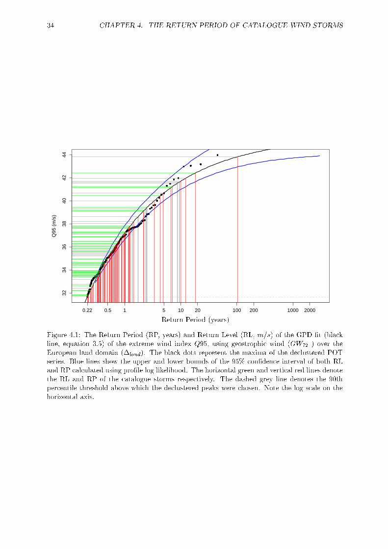
34 CHAPTER 4. THE RETURN PERIOD OF CATALOGUE WIND STORMS
T
Q95
(m
/s)
3234
3638
4042
44
0.22 0.5 1 5 10 20 100 200 1000 2000
POT − PRE_storms , Thresh 0.9 Region: −35,30,35,73, land_only
(Index: wQ95 − Gesostrophic Wind [850 hPa]− Decl.Meth.: FS.daily.u)Return Period (years)
Figure 4.1: The Return Period (RP, years) and Return Level (RL, m=s) of the GPD �t (blackline, equation 3.5) of the extreme wind index Q95, using geostrophic wind (GW72 ) over theEuropean land domain (�land). The black dots represent the maxima of the declustered POTseries. Blue lines show the upper and lower bounds of the 95% con�dence interval of both RLand RP calculated using pro�le log likelihood. The horizontal green and vertical red lines denotethe RL and RP of the catalogue storms respectively. The dashed grey line denotes the 90thpercentile threshold above which the declustered peaks were chosen. Note the log scale on thehorizontal axis.

4.1. THE EXTREME WIND DISTRIBUTION BASED ON EXTREME WIND INDICES 35
represents the range of possible RPs well, i.e. the catalogue storms in many cases coincide withthe plotting points (the cluster maxima) of the ERA-40 derived EWI. There are storms thatappear in the ERA-40 EWI which are not included in the storm catalogue. Notice that theindex SQ95 performs poorly in terms of capturing the severity of the catalogue storms over alldomains. Nonetheless we considered it important to show the results of this index to highlightthat some EWI are better than others in capturing the storminess of a region. In some plots it isclear that the GPD �t is not optimal, for example in �gure 4.5f) and i) where the 95% con�denceinterval does not contain the plotting points in the middle section of the GPD �t (1-10 years).This is also evident, for land only areas, in the qq-plots shown in �gure 4.4. As explained above,this could be due to choosing a threshold which is not high enough to justify using the GPD ordue to the method we used to decluster the data. A comparison between qq-plots for a speci�cEWI reveals dependence of the GPD �t quality on the declustering method chosen (�gure 4.6aand b). Although, practically this has had no major in�uence on the RP estimates (�gure 4.6c).

36 CHAPTER 4. THE RETURN PERIOD OF CATALOGUE WIND STORMS
WG72 GW72
m=s
a)T
17.0
17.5
18.0
18.5
19.0
19.5
20.0
20.5
0.28 0.5 1 5 10 20 100 200 1000 2000
POT − PRE_storms , Thresh 0.9 Region: −35,30,35,73, all_gp
(Index: wMean − Wind Gust (10m)− Decl.Meth.: FS.daily.u)
b)T
Q95
(m
/s)
2021
2223
2425
26
0.27 0.5 1 5 10 20 100 200 1000 2000
POT − PRE_storms , Thresh 0.9 Region: −35,30,35,73, all_gp
(Index: wMean − Gesostrophic Wind [850 hPa]− Decl.Meth.: FS.daily.u)
m=s
c)T
3032
3436
0.26 0.5 1 5 10 20 100 200 1000 2000
POT − PRE_storms , Thresh 0.9 Region: −35,30,35,73, all_gp
(Index: wQ95 − Wind Gust (10m)− Decl.Meth.: FS.daily.u)
d)T
Q95
(m
/s)
4045
5055
0.23 0.5 1 5 10 20 100 200 1000 2000
POT − PRE_storms , Thresh 0.9 Region: −35,30,35,73, all_gp
(Index: wQ95 − Gesostrophic Wind [850 hPa]− Decl.Meth.: FS.daily.u)
Sum
m=s
e)T
1800
020
000
2200
024
000
0.16 0.5 1 5 10 20 100 200 1000 2000
POT − PRE_storms , Thresh 0.9 Region: −35,30,35,73, all_gp
(Index: S_gr_wQ95 − Wind Gust (10m)− Decl.Meth.: FS.daily.u)
f)T
Q95
(m
/s)
2500
030
000
3500
040
000
0.19 0.5 1 5 10 20 100 200 1000 2000
POT − PRE_storms , Thresh 0.9 Region: −35,30,35,73, all_gp
(Index: S_gr_wQ95 − Gesostrophic Wind [850 hPa]− Decl.Meth.: FS.daily.u)
Sum
m=s
g)T
2500
3000
3500
4000
4500
0.25 0.5 1 5 10 20 100 200 1000 2000
POT − PRE_storms , Thresh 0.9 Region: −35,30,35,73, all_gp
(Index: wS_frac_q95 − Wind Gust (10m)− Decl.Meth.: FS.daily.u)
h)T
Q95
(m
/s)
3000
3500
4000
4500
5000
5500
6000
0.25 0.5 1 5 10 20 100 200 1000 2000
POT − PRE_storms , Thresh 0.9 Region: −35,30,35,73, all_gp
(Index: wS_frac_q95 − Gesostrophic Wind [850 hPa]− Decl.Meth.: FS.daily.u)
Sum
m=s
i)T
2000
2500
3000
3500
4000
4500
5000
0.25 0.5 1 5 10 20 100 200 1000 2000
POT − PRE_storms , Thresh 0.9 Region: −35,30,35,73, all_gp
(Index: wS_frac_Dq99_95 − Wind Gust (10m)− Decl.Meth.: FS.daily.u)
j)T
Q95
(m
/s)
3000
4000
5000
6000
0.25 0.5 1 5 10 20 100 200 1000 2000
POT − PRE_storms , Thresh 0.9 Region: −35,30,35,73, all_gp
(Index: wS_frac_Dq99_95 − Gesostrophic Wind [850 hPa]− Decl.Meth.: FS.daily.u)Return Period (years) Return Period (years)
Figure 4.2: The RP and RL of the GPD �t to the �ve EWIs calculated over the whole domain.RL (m=s, vertical axis) versus RP (years, horizontal axis) with uncertainty (pro�le log likelihood)estimates. Indices based on WG72 and �all�masked (left column) and indices based on GW72
and �all (right column). a) and b) �X, c) and d) Q95, e) and f) SQ95, g) and h) Sfq95, i) and j)Sfq95q99. Green and red lines indicate the RL and RP of the the 96 PartnerRe storms withinthe ONDJFMA season. The dashed grey line denotes the 90th percentile threshold above whichthe declustered peaks were chosen.

4.1. THE EXTREME WIND DISTRIBUTION BASED ON EXTREME WIND INDICES 37
WG72 GW72
m=s
a)T
1314
1516
17
0.23 0.5 1 5 10 20 100 200 1000 2000
POT − PRE_storms , Thresh 0.9 Region: −35,30,35,73, land_only
(Index: wMean − Wind Gust (10m)− Decl.Meth.: FS.daily.u)
b)T
Q95
(m
/s)
1820
2224
2628
0.23 0.5 1 5 10 20 100 200 1000 2000
POT − PRE_storms , Thresh 0.9 Region: −35,30,35,73, land_only
(Index: wMean − Gesostrophic Wind [850 hPa]− Decl.Meth.: FS.daily.u)
m=s
c)T
1920
2122
2324
2526
0.29 0.5 1 5 10 20 100 200 1000 2000
POT − PRE_storms , Thresh 0.9 Region: −35,30,35,73, land_only
(Index: wQ95 − Wind Gust (10m)− Decl.Meth.: FS.daily.u)
d)T
Q95
(m
/s)
3234
3638
4042
44
0.22 0.5 1 5 10 20 100 200 1000 2000
POT − PRE_storms , Thresh 0.9 Region: −35,30,35,73, land_only
(Index: wQ95 − Gesostrophic Wind [850 hPa]− Decl.Meth.: FS.daily.u)
Sum
m=s
e)T
2600
2800
3000
3200
3400
3600
0.22 0.5 1 5 10 20 100 200 1000 2000
POT − PRE_storms , Thresh 0.9 Region: −35,30,35,73, land_only
(Index: S_gr_wQ95 − Wind Gust (10m)− Decl.Meth.: FS.daily.u)
f)T
Q95
(m
/s)
8000
9000
1000
011
000
1200
013
000
1400
0
0.17 0.5 1 5 10 20 100 200 1000 2000
POT − PRE_storms , Thresh 0.9 Region: −35,30,35,73, land_only
(Index: S_gr_wQ95 − Gesostrophic Wind [850 hPa]− Decl.Meth.: FS.daily.u)
Sum
m=s
g)T
800
1000
1200
1400
1600
0.22 0.5 1 5 10 20 100 200 1000 2000
POT − PRE_storms , Thresh 0.9 Region: −35,30,35,73, land_only
(Index: wS_frac_q95 − Wind Gust (10m)− Decl.Meth.: FS.daily.u)
h)T
Q95
(m
/s)
1500
2000
2500
0.22 0.5 1 5 10 20 100 200 1000 2000
POT − PRE_storms , Thresh 0.9 Region: −35,30,35,73, land_only
(Index: wS_frac_q95 − Gesostrophic Wind [850 hPa]− Decl.Meth.: FS.daily.u)
Sum
m=s
i)T
1000
1500
2000
0.23 0.5 1 5 10 20 100 200 1000 2000
POT − PRE_storms , Thresh 0.9 Region: −35,30,35,73, land_only
(Index: wS_frac_Dq99_95 − Wind Gust (10m)− Decl.Meth.: FS.daily.u)
j)T
Q95
(m
/s)
1000
1500
2000
2500
3000
3500
0.23 0.5 1 5 10 20 100 200 1000 2000
POT − PRE_storms , Thresh 0.9 Region: −35,30,35,73, land_only
(Index: wS_frac_Dq99_95 − Gesostrophic Wind [850 hPa]− Decl.Meth.: FS.daily.u)Return Period (years) Return Period (years)
Figure 4.3: The RP and RL of the GPD �t to the �ve EWIs calculated over land. RL (m=s,vertical axis) versus RP (years, horizontal axis) with uncertainty (pro�le log likelihood) estimates.Indices based on WG72 and �land�masked (left column) and indices based on W 850
72geo and �land
(right column). a) and b) �X, c) and d) Q95, e) and f) SQ95, g) and h) Sfq95, i) and j)Sfq95q99. Green and red lines indicate the RL and RP of the the 96 PartnerRe storms withinthe ONDJFMA season. The dashed grey line denotes the 90th percentile threshold above whichthe declustered peaks were chosen.
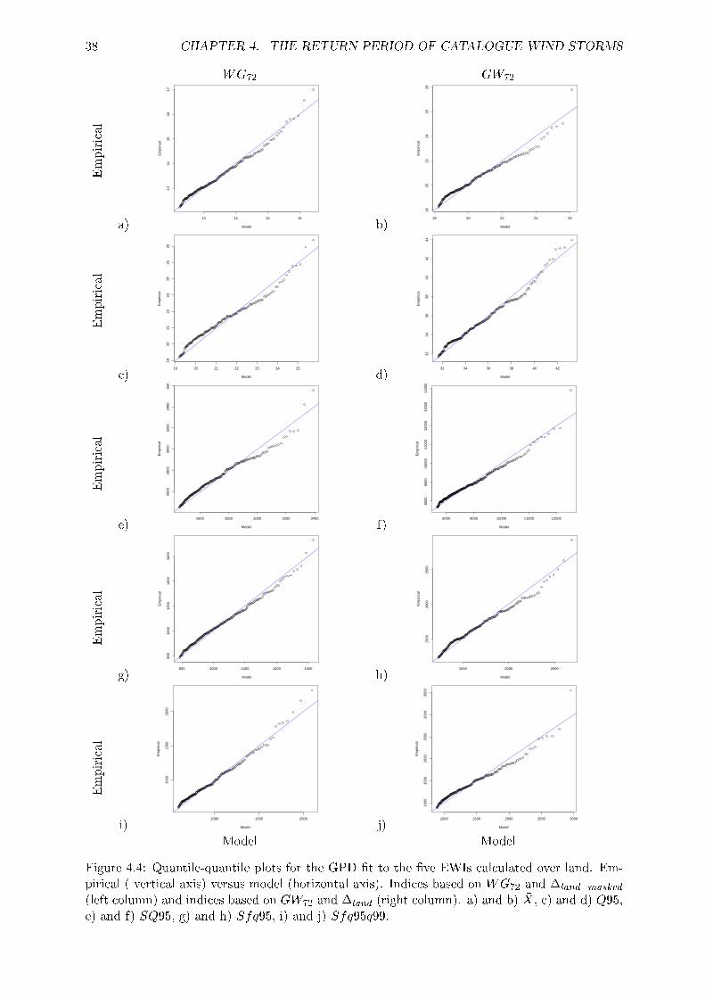
38 CHAPTER 4. THE RETURN PERIOD OF CATALOGUE WIND STORMS
WG72 GW72
Empirical
a)13 14 15 16
1314
1516
17
Quantile Plot
Model
Em
piric
al
QQ−Plot, Thresh 0.9 Region: −35,30,35,73, land_only
(Index: wMean − Wind Gust (10m)− Decl.Meth.: FS.daily.u)b)
18 20 22 24 26
1820
2224
2628
Quantile Plot
Model
Em
piric
al
QQ−Plot, Thresh 0.9 _du_ 0.9 Region: −35,30,35,73, land_only
(Index: wMean − Geostrophic Wind (850 hPa)− Decl.Meth.: FS.daily.u)
Empirical
c)19 20 21 22 23 24 25
1920
2122
2324
2526
Quantile Plot
Model
Em
piric
al
QQ−Plot, Thresh 0.9 Region: −35,30,35,73, land_only
(Index: wQ95 − Wind Gust (10m)− Decl.Meth.: FS.daily.u)d)
32 34 36 38 40 42
3234
3638
4042
44
Quantile Plot
Model
Em
piric
al
QQ−Plot, Thresh 0.9 _du_ 0.9 Region: −35,30,35,73, land_only
(Index: wQ95 − Geostrophic Wind (850 hPa)− Decl.Meth.: FS.daily.u)
Empirical
e)2600 2800 3000 3200 3400
2600
2800
3000
3200
3400
3600
Quantile Plot
Model
Em
piric
al
QQ−Plot, Thresh 0.9 Region: −35,30,35,73, land_only
(Index: S_gr_wQ95 − Wind Gust (10m)− Decl.Meth.: FS.daily.u)f)
8000 9000 10000 11000 12000
8000
9000
1000
011
000
1200
013
000
1400
0
Quantile Plot
Model
Em
piric
al
QQ−Plot, Thresh 0.9 _du_ 0.9 Region: −35,30,35,73, land_only
(Index: S_gr_wQ95 − Geostrophic Wind (850 hPa)− Decl.Meth.: FS.daily.u)
Empirical
g)800 1000 1200 1400 1600
800
1000
1200
1400
1600
Quantile Plot
Model
Em
piric
al
QQ−Plot, Thresh 0.9 Region: −35,30,35,73, land_only
(Index: wS_frac_q95 − Wind Gust (10m)− Decl.Meth.: FS.daily.u)h)
1500 2000 2500
1500
2000
2500
Quantile Plot
Model
Em
piric
al
QQ−Plot, Thresh 0.9 _du_ 0.9 Region: −35,30,35,73, land_only
(Index: wS_frac_q95 − Geostrophic Wind (850 hPa)− Decl.Meth.: FS.daily.u)
Empirical
i)1000 1500 2000
1000
1500
2000
Quantile Plot
Model
Em
piric
al
QQ−Plot, Thresh 0.9 Region: −35,30,35,73, land_only
(Index: wS_frac_Dq99_95 − Wind Gust (10m)− Decl.Meth.: FS.daily.u)j)
1000 1500 2000 2500 3000
1000
1500
2000
2500
3000
3500
Quantile Plot
Model
Em
piric
al
QQ−Plot, Thresh 0.9 _du_ 0.9 Region: −35,30,35,73, land_only
(Index: wS_frac_Dq99_95 − Geostrophic Wind (850 hPa)− Decl.Meth.: FS.daily.u)
Model Model
Figure 4.4: Quantile-quantile plots for the GPD �t to the �ve EWIs calculated over land. Em-pirical ( vertical axis) versus model (horizontal axis). Indices based on WG72 and �land�masked
(left column) and indices based on GW72 and �land (right column). a) and b) �X, c) and d) Q95,e) and f) SQ95, g) and h) Sfq95, i) and j) Sfq95q99.
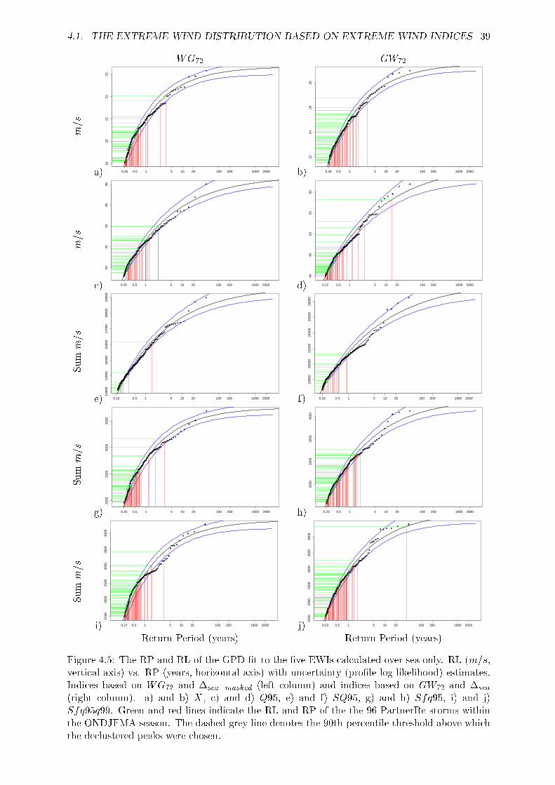
4.1. THE EXTREME WIND DISTRIBUTION BASED ON EXTREME WIND INDICES 39
WG72 GW72
m=s
a)T
1920
2122
23
0.26 0.5 1 5 10 20 100 200 1000 2000
POT − PRE_storms , Thresh 0.9 Region: −35,30,35,73, sea_only
(Index: wMean − Wind Gust (10m)− Decl.Meth.: FS.daily.u)
b)T
Q95
(m
/s)
2224
2628
0.26 0.5 1 5 10 20 100 200 1000 2000
POT − PRE_storms , Thresh 0.9 Region: −35,30,35,73, sea_only
(Index: wMean − Gesostrophic Wind [850 hPa]− Decl.Meth.: FS.daily.u)
m=s
c)T
3032
3436
38
0.25 0.5 1 5 10 20 100 200 1000 2000
POT − PRE_storms , Thresh 0.9 Region: −35,30,35,73, sea_only
(Index: wQ95 − Wind Gust (10m)− Decl.Meth.: FS.daily.u)
d)T
Q95
(m
/s)
4045
5055
60
0.22 0.5 1 5 10 20 100 200 1000 2000
POT − PRE_storms , Thresh 0.9 Region: −35,30,35,73, sea_only
(Index: wQ95 − Gesostrophic Wind [850 hPa]− Decl.Meth.: FS.daily.u)
Sum
m=s
e)T
1300
014
000
1500
016
000
1700
018
000
1900
0
0.16 0.5 1 5 10 20 100 200 1000 2000
POT − PRE_storms , Thresh 0.9 Region: −35,30,35,73, sea_only
(Index: S_gr_wQ95 − Wind Gust (10m)− Decl.Meth.: FS.daily.u)
f)T
Q95
(m
/s)
1800
020
000
2200
024
000
2600
028
000
0.19 0.5 1 5 10 20 100 200 1000 2000
POT − PRE_storms , Thresh 0.9 Region: −35,30,35,73, sea_only
(Index: S_gr_wQ95 − Gesostrophic Wind [850 hPa]− Decl.Meth.: FS.daily.u)
Sum
m=s
g)T
2000
2500
3000
3500
0.25 0.5 1 5 10 20 100 200 1000 2000
POT − PRE_storms , Thresh 0.9 Region: −35,30,35,73, sea_only
(Index: wS_frac_q95 − Wind Gust (10m)− Decl.Meth.: FS.daily.u)
h)T
Q95
(m
/s)
2500
3000
3500
4000
0.23 0.5 1 5 10 20 100 200 1000 2000
POT − PRE_storms , Thresh 0.9 Region: −35,30,35,73, sea_only
(Index: wS_frac_q95 − Gesostrophic Wind [850 hPa]− Decl.Meth.: FS.daily.u)
Sum
m=s
i)T
1500
2000
2500
3000
3500
4000
0.27 0.5 1 5 10 20 100 200 1000 2000
POT − PRE_storms , Thresh 0.9 Region: −35,30,35,73, sea_only
(Index: wS_frac_Dq99_95 − Wind Gust (10m)− Decl.Meth.: FS.daily.u)
j)T
Q95
(m
/s)
1500
2000
2500
3000
3500
4000
0.23 0.5 1 5 10 20 100 200 1000 2000
POT − PRE_storms , Thresh 0.9 Region: −35,30,35,73, sea_only
(Index: wS_frac_Dq99_95 − Gesostrophic Wind [850 hPa]− Decl.Meth.: FS.daily.u)Return Period (years) Return Period (years)
Figure 4.5: The RP and RL of the GPD �t to the �ve EWIs calculated over sea only. RL (m=s,vertical axis) vs. RP (years, horizontal axis) with uncertainty (pro�le log likelihood) estimates.Indices based on WG72 and �sea�masked (left column) and indices based on GW72 and �sea
(right column). a) and b) �X, c) and d) Q95, e) and f) SQ95, g) and h) Sfq95, i) and j)Sfq95q99. Green and red lines indicate the RL and RP of the the 96 PartnerRe storms withinthe ONDJFMA season. The dashed grey line denotes the 90th percentile threshold above whichthe declustered peaks were chosen.

40 CHAPTER 4. THE RETURN PERIOD OF CATALOGUE WIND STORMS
a)
32 34 36 38 40 42 44
3234
3638
4042
44
Quantile Plot
Model
Em
piric
al
QQ−Plot extRemes.runs.fixed.u , Thresh 0.9 Region: −35,30,35,73, land_only
(Index: wQ95 − Wind Gust (10m)− Decl.Meth.: extRemes.runs.fixed.u)
b)
19 20 21 22 23 24 25
1920
2122
2324
2526
Quantile Plot
Model
Em
piric
al
QQ−Plot, Thresh 0.9 Region: −35,30,35,73, land_only
(Index: wQ95 − Wind Gust (10m)− Decl.Meth.: FS.daily.u)
c)Return periods FS [years]
Ret
urn
perio
ds r
uns
[yea
rs]
0.5 1 5 10 20 50 100 200 500
0.5
15
1020
5010
020
050
0
Return Periods FS vs. runs (Index: land_wQ95 )
Threshold: 0.9, Spearman−Cor: 1_Kendall Tau−Cor: 1
Figure 4.6: Comparison of the �tted GPD using runs declustering and the Ferro and Segers method.
Quantile-quantile plot of Q95, WG72, �land using runs declustering a) and Ferro and Segers (2003) b).
In c) a scatter plot of the RPs of catalogue storms comparing the two methods. Note the logarithmic
scale. 95% con�dence intervals for each of the RP are denoted by orange (Ferro and Segers, 2003) and
blue (runs declustering) whiskers on each scatter plot point. Solid black line denotes the equal RP line.
At the bottom of each sub-�gure is the Spearman rank and Kendall's Tau correlation coe�cient.
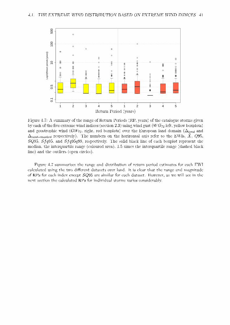
4.1. THE EXTREME WIND DISTRIBUTION BASED ON EXTREME WIND INDICES 41
Log1
0(R
etur
n pe
riods
[yea
rs])
1 2 3 4 5 1 2 3 4 5
0.1
0.5
1010
050
0
Indices WG vs. GWS − land
Return Period (years)
Figure 4.7: A summary of the range of Return Periods (RP, years) of the catalogue storms givenby each of the �ve extreme wind indices (section 2.3) using wind gust (WG72 left, yellow boxplots)and geostrophic wind (GW72, right, red boxplots) over the European land domain (�land and�land�masked respectively). The numbers on the horizontal axis refer to the EWIs, �X, Q95,SQ95, Sfq95, and Sfq95q99, respectively. The solid black line of each boxplot represent themedian, the interquartile range (coloured area), 1.5 times the interquartile range (dashed blackline) and the outliers (open circles).
Figure 4.7 summarises the range and distribution of return period estimates for each EWIcalculated using the two di�erent datasets over land. It is clear that the range and magnitudeof RPs for each index except SQ95 are similar for each dataset. However, as we will see in thenext section the calculated RPs for individual storms varies considerably.

42 CHAPTER 4. THE RETURN PERIOD OF CATALOGUE WIND STORMS
We wished to investigate what e�ect the use of either WG72 or GW72 had on the RPsestimated from the derived EWI. Figures 4.8 to 4.12 present scatter plots of the RPs of thePartnerRe storms estimated using WG72 versus the RPs using GW72 for each index and for eachof the domains, all grid points, land only and sea only. On each plot there are 96 points (thenumber of catalogue storms in the October - April season). For each point the 95% con�denceinterval for each RP is shown in either red (WG72) or blue (GW72). Generally, there are poorrelationships between the RPs of the catalogue storms calculated using the extreme indices andWG72 and GW72. In �gures 4.8a to 4.12a, (�all�masked and �all), we can see that the RPs ofthe catalogue storms are generally higher when calculated from GW72. When considering landonly (�land�masked and �land) RP relationships (�gures 4.8b to 4.12b) there are generally higherRPs estimated for the storms but also a larger di�erence in the RP of each storm not explainedby the uncertainty of the EVA. For example, in �gure 4.9b there is a storm which has a RPestimate of approximately 70 years using Q95, WG72 whereas the same storm using Q95, GW72
is only estimated to be 2 year RP event. The relationship between the SQ95, again is clearly theworst performing EWI. We discuss the potential causes of these discrepancies later in the report.There is generally a tighter grouping of the RP estimates when sea only grid points are used(�sea�masked and �sea, �gures 4.8c to 4.12c), however, even though the RPs are lower in manycases the di�erences in the RPs cannot be explained by the GPD �t uncertainty. In many of the�gures it is evident that some storms have the lowest return period possible (approximately 0.3years or lower). Any storm which was not above the �xed POT threshold was given the samereturn period of 1=� as explained in section 3.3.
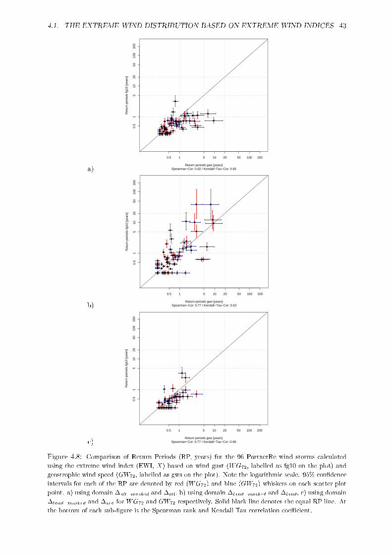
4.1. THE EXTREME WIND DISTRIBUTION BASED ON EXTREME WIND INDICES 43
a)Return periods gws [years]
Ret
urn
perio
ds fg
10 [y
ears
]
0.5 1 5 10 20 50 100 200
0.5
15
1020
5010
020
0
Return Periods gws vs. fg10 (Index: all_wMean )
Spearman−Cor: 0.82 / Kendall−Tau−Cor: 0.65
b)Return periods gws [years]
Ret
urn
perio
ds fg
10 [y
ears
]
0.5 1 5 10 20 50 100 200
0.5
15
1020
5010
020
0
Return Periods gws vs. fg10 (Index: land_wMean )
Spearman−Cor: 0.77 / Kendall−Tau−Cor: 0.63
c)Return periods gws [years]
Ret
urn
perio
ds fg
10 [y
ears
]
0.5 1 5 10 20 50 100 200
0.5
15
1020
5010
020
0
Return Periods gws vs. fg10 (Index: sea_wMean )
Spearman−Cor: 0.77 / Kendall−Tau−Cor: 0.68
Figure 4.8: Comparison of Return Periods (RP, years) for the 96 PartnerRe wind storms calculated
using the extreme wind index (EWI, �X) based on wind gust (WG72, labelled as fg10 on the plot) and
geostrophic wind speed (GW72, labelled as gws on the plot). Note the logarithmic scale. 95% con�dence
intervals for each of the RP are denoted by red (WG72) and blue (GW72) whiskers on each scatter plot
point. a) using domain �all�masked and �all; b) using domain �land�masked and �land, c) using domain
�land�masked and �sea for WG72 and GW72 respectively. Solid black line denotes the equal RP line. At
the bottom of each sub-�gure is the Spearman rank and Kendall Tau correlation coe�cient.

44 CHAPTER 4. THE RETURN PERIOD OF CATALOGUE WIND STORMS
a)Return periods gws [years]
Ret
urn
perio
ds fg
10 [y
ears
]
0.5 1 5 10 20 50 100 200
0.5
15
1020
5010
020
0
Return Periods gws vs. fg10 (Index: all_wQ95 )
Spearman−Cor: 0.77 / Kendall−Tau−Cor: 0.64
b)Return periods gws [years]
Ret
urn
perio
ds fg
10 [y
ears
]
0.5 1 5 10 20 50 100 200
0.5
15
1020
5010
020
0
Return Periods gws vs. fg10 (Index: land_wQ95 )
Spearman−Cor: 0.56 / Kendall−Tau−Cor: 0.41
c)Return periods gws [years]
Ret
urn
perio
ds fg
10 [y
ears
]
0.5 1 5 10 20 50 100 200
0.5
15
1020
5010
020
0
Return Periods gws vs. fg10 (Index: sea_wQ95 )
Spearman−Cor: 0.71 / Kendall−Tau−Cor: 0.61
Figure 4.9: As for �gure 4.8 but using Q95

4.1. THE EXTREME WIND DISTRIBUTION BASED ON EXTREME WIND INDICES 45
a)Return periods gws [years]
Ret
urn
perio
ds fg
10 [y
ears
]
0.5 1 5 10 20 50 100 200
0.5
15
1020
5010
020
0
Return Periods gws vs. fg10 (Index: all_S_gr_wQ95 )
Spearman−Cor: 0.49 / Kendall−Tau−Cor: 0.48
b)Return periods gws [years]
Ret
urn
perio
ds fg
10 [y
ears
]
0.5 1 5 10 20 50 100 200
0.5
15
1020
5010
020
0
Return Periods gws vs. fg10 (Index: land_S_gr_wQ95 )
Spearman−Cor: 0.43 / Kendall−Tau−Cor: 0.36
c)Return periods gws [years]
Ret
urn
perio
ds fg
10 [y
ears
]
0.5 1 5 10 20 50 100 200
0.5
15
1020
5010
020
0
Return Periods gws vs. fg10 (Index: sea_S_gr_wQ95 )
Spearman−Cor: 0.43 / Kendall−Tau−Cor: 0.42
Figure 4.10: As for �gure 4.8 but using SQ95

46 CHAPTER 4. THE RETURN PERIOD OF CATALOGUE WIND STORMS
a)Return periods gws [years]
Ret
urn
perio
ds fg
10 [y
ears
]
0.5 1 5 10 20 50 100 200
0.5
15
1020
5010
020
0
Return Periods gws vs. fg10 (Index: all_frac_q95 )
Spearman−Cor: 0.81 / Kendall−Tau−Cor: 0.65
b)Return periods gws [years]
Ret
urn
perio
ds fg
10 [y
ears
]
0.5 1 5 10 20 50 100 200
0.5
15
1020
5010
020
0
Return Periods gws vs. fg10 (Index: land_frac_q95 )
Spearman−Cor: 0.72 / Kendall−Tau−Cor: 0.59
c)Return periods gws [years]
Ret
urn
perio
ds fg
10 [y
ears
]
0.5 1 5 10 20 50 100 200
0.5
15
1020
5010
020
0
Return Periods gws vs. fg10 (Index: sea_frac_q95 )
Spearman−Cor: 0.82 / Kendall−Tau−Cor: 0.7
Figure 4.11: As for �gure 4.8 but using Sfq95
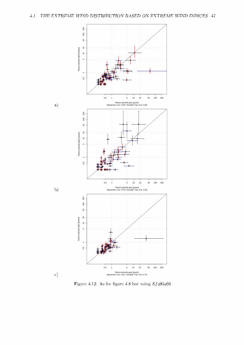
4.1. THE EXTREME WIND DISTRIBUTION BASED ON EXTREME WIND INDICES 47
a)Return periods gws [years]
Ret
urn
perio
ds fg
10 [y
ears
]
0.5 1 5 10 20 50 100 200
0.5
15
1020
5010
020
0
Return Periods gws vs. fg10 (Index: all_frac_Dq99_95 )
Spearman−Cor: 0.83 / Kendall−Tau−Cor: 0.66
b)Return periods gws [years]
Ret
urn
perio
ds fg
10 [y
ears
]
0.5 1 5 10 20 50 100 200
0.5
15
1020
5010
020
0
Return Periods gws vs. fg10 (Index: land_frac_Dq99_95 )
Spearman−Cor: 0.78 / Kendall−Tau−Cor: 0.65
c)Return periods gws [years]
Ret
urn
perio
ds fg
10 [y
ears
]
0.5 1 5 10 20 50 100 200
0.5
15
1020
5010
020
0
Return Periods gws vs. fg10 (Index: sea_frac_Dq99_95 )
Spearman−Cor: 0.91 / Kendall−Tau−Cor: 0.79
Figure 4.12: As for �gure 4.8 but using Sfq95q99

48 CHAPTER 4. THE RETURN PERIOD OF CATALOGUE WIND STORMS
We summarise the e�ects of using di�erent wind data and di�erent EWIs to estimate theRPs of the catalogue storms using the Spearman rank correlation coe�cient. In table 4.1 wepresent the Spearman rank correlation between RPs calculated for each possible combination ofEWI, wind data and mask. The results are varied, with some EWI, data and mask combinationsresulting in very similar RP estimates, while others are very di�erent from one another. Fromsuch an analysis is it hard to extract information on the relative e�ects that EWI, base data andmask have on the RP estimates, nonetheless we highlight some of the results of this analysis.Inter-index comparisons show that �X, Sfq95 and Sfq95q99 are the most highly correlatedwith each other for both data sets (WG72 and GW72) and for all masks. Inter-dataset indiceswhich show the highest correlations are �X, Sfq95, Sfq95q99. Note that the highest inter-index correlations are higher than the highest inter-dataset correlations, indicating that greaterdi�erences between RP estimates are due to the dataset rather than the best EWIs shown here.However, if we consider the indices �X and Q95 only we see that the inter-dataset correlationsare higher than the inter-index correlations. This highlights the di�culty in trying to establishthe main cause for the di�erences in the RP estimates.
We tried to isolate the e�ect of using the mask on WG72 (land only) by comparing the GW72
masked and unmasked RP estimates. Firstly we recall the comparison between the RPs usingWG72, �land�masked and GW72, �land and we see that the their is a fair relationship betweenthe two data sets (�gure 4.13a). If we mask the GW72 as if it were WG72 with �land�masked andcompare the RPs we can see a slight improvement of the Spearman rank correlation from 0.55to 0.66 (�gure 4.13b). However, the main cause for the discrepancies in the RPs is due to thebase data set and not the application of the mask as demonstrated by �gure 4.13c where we seethat the correlation between GW72, �land�masked and GW72, �land is much higher (0.86).

4.1. THE EXTREME WIND DISTRIBUTION BASED ON EXTREME WIND INDICES 49
AL
L
WG
_w
Me
an
WG
_w
Q9
5
WG
_S
_g
r_w
Q9
5
WG
_w
Sf_
q9
5
WG
_w
Sf_
q9
5_
99
GW
_w
Me
an
GW
_w
Q9
5
GW
_S
_g
r_w
Q9
5
GW
_w
Sf_
q9
5
GW
_w
Sf_
q9
5_
99
WG_wMean 1
WG_wQ95 0.63 1
WG_S_gr_wQ95 0.018 0.307 1
WG_wSf_q95 0.914 0.519 -0.096 1
WG_wSf_q95_99 0.879 0.699 0.071 0.894 1
GW_wMean 0.823 0.453 -0.075 0.823 0.763 1
GW_wQ95 0.701 0.772 0.132 0.586 0.705 0.637 1
GW_S_gr_wQ95 0.253 0.605 0.488 0.155 0.311 0.071 0.447 1
GW_wSf_q95 0.728 0.398 -0.095 0.807 0.742 0.933 0.526 -0.004 1
GW_wSf_q95_99 0.727 0.543 -0.001 0.762 0.83 0.865 0.703 0.188 0.883 1
LA
ND
WG
_w
Me
an
WG
_w
Q9
5
WG
_S
_g
r_w
Q9
5
WG
_w
Sf_
q9
5
WG
_w
Sf_
q9
5_
99
GW
_w
Me
an
GW
_w
Q9
5
GW
_S
_g
r_w
Q9
5
GW
_w
Sf_
q9
5
GW
_w
Sf_
q9
5_
99
WG_wMean 1
WG_wQ95 0.591 1
WG_S_gr_wQ95 0.391 0.715 1
WG_wSf_q95 0.936 0.523 0.382 1
WG_wSf_q95_99 0.95 0.583 0.438 0.953 1
GW_wMean 0.765 0.461 0.215 0.731 0.733 1
GW_wQ95 0.628 0.557 0.23 0.586 0.628 0.687 1
GW_S_gr_wQ95 -0.007 0.214 0.429 0.027 0.037 -0.059 0.126 1
GW_wSf_q95 0.739 0.459 0.243 0.72 0.72 0.962 0.65 -0.034 1
GW_wSf_q95_99 0.763 0.487 0.317 0.752 0.775 0.909 0.737 0.063 0.915 1
SE
A
WG
_w
Me
an
WG
_w
Q9
5
WG
_S
_g
r_w
Q9
5
WG
_w
Sf_
q9
5
WG
_w
Sf_
q9
5_
99
GW
_w
Me
an
GW
_w
Q9
5
GW
_S
_g
r_w
Q9
5
GW
_w
Sf_
q9
5
GW
_w
Sf_
q9
5_
99
WG_wMean 1
WG_wQ95 0.563 1
WG_S_gr_wQ95 0.144 0.256 1
WG_wSf_q95 0.873 0.556 -0.014 1
WG_wSf_q95_99 0.8 0.764 0.174 0.853 1
GW_wMean 0.773 0.496 -0.008 0.787 0.749 1
GW_wQ95 0.638 0.709 0.045 0.63 0.714 0.664 1
GW_S_gr_wQ95 0.321 0.597 0.429 0.267 0.445 0.205 0.352 1
GW_wSf_q95 0.754 0.528 0.011 0.822 0.782 0.934 0.606 0.219 1
GW_wSf_q95_99 0.704 0.694 0.124 0.762 0.908 0.834 0.745 0.348 0.865 1
Table 4.1: The Spearman rank correlation between the Return Periods (RP) of catalogue storms(96 storms) calculated from di�erent extreme wind indices (EWI, yellow shaded boxes, alsodescribed as inter -index ) and di�erent datasets (either WG72or GW72, red shaded boxes, alsodescribed as inter-dataset) over all grid points a), land only grid points b) and sea only gridpoints c). The labels �WG� and �GW� refer to wind gust and geostrophic wind respectively. Thelabelling of the EWIs is di�erent to that in the text, however the order of the indices is the sameas the order given in section 2.3.

50 CHAPTER 4. THE RETURN PERIOD OF CATALOGUE WIND STORMS
a)Return periods gws [years]
Ret
urn
perio
ds fg
10 [y
ears
]
0.5 1 5 10 20 50 100 200
0.5
15
1020
5010
020
0
Return Periods gws vs. fg10 (Index: land_wQ95 )
Spearman−Cor: 0.56 / Kendall−Tau−Cor: 0.41
b)Return periods gws [years]
Ret
urn
perio
ds fg
10 [y
ears
]
0.5 1 5 10 20 50 100 200
0.5
15
1020
5010
020
0
Return Periods (Masked) gws vs. fg10 (Index: land_wQ95 )
Spearman−Cor: 0.66 / Kendall−Tau−Cor: 0.49
c)Return periods gws.no.mask [years]
Ret
urn
perio
ds g
ws.
mas
k [y
ears
]
0.5 1 5 10 20 50 100 200
0.5
15
1020
5010
020
0
Return Periods gws.no.mask vs. gws.mask (Index: land_wQ95 )
Spearman−Cor: 0.85 / Kendall−Tau−Cor: 0.71
Figure 4.13: The e�ect of masking unrealistic wind gust grid points on return period estimates. Scat-
ter plot of RPs (years) for the 96 catalogue wind storms calculated using Q95, WG72 versus the RPs
calculated using Q95, GW72. a) using domain �land�masked and �land; b) using domain �land�masked
and �land�masked for WG72 and GW72 respectively and c) using GW72 domain �land�masked and �land.
Solid black line denotes the equal RP line. Note the logarithmic scale. 95% con�dence intervals for each
of the RP are denoted by red and blue (green and orange) for WG72and GW72 in a) and b) and in c)
the colours brown and purple are used to denote the RP con�dence intervals of GW72 �land�masked and
�land respectively. At the bottom of each sub-�gure is the Spearman rank and Kendall Tau correlation
coe�cient.
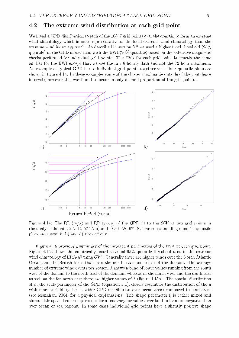
4.2. THE EXTREME WIND DISTRIBUTION AT EACH GRID POINT 51
4.2 The extreme wind distribution at each grid point
We �tted a GPD distribution to each of the 10857 grid points over the domain to form an extremewind climatology which is more representative of the local extreme wind climatology than theextreme wind index approach. As described in section 3.2 we used a higher �xed threshold (95%quantile) in the GPD model than with the EWI (90% quantile) based on the extensive diagnosticchecks performed for individual grid points. The EVA for each grid point is exactly the sameas that for the EWI except that we use the raw 6 hourly data and not the 72 hour maximum.An example of typical GPD �ts to individual grid points together with their quantile plots areshown in �gure 4.14. In these examples some of the cluster maxima lie outside of the con�denceintervals, however this was found to occur in only a small proportion of the grid points .
m=s
a)T
(m/s
)
2025
3035
4045
50
0.5 1 5 10 20 100 200 1000 2000
POT − PRe Thresh 0.95 _daily_th 0.9
Control for gp: gp_2.5_57
b)25 30 35 40 45 50
2530
3540
4550
Quantile Plot
ModelE
mpi
rical
QQ−Plot, Thresh 0.95 _du_ 0.9
(Gridpoint: gp_2.5_57 / dc.Method: FS.daily.u )
m=s
c)T
(m/s
)
2025
3035
40
0.5 1 5 10 20 100 200 1000 2000
POT − PRe Thresh 0.95 _daily_th 0.9
Control for gp: gp_30_67
d)20 25 30 35
2025
3035
40
Quantile Plot
Model
Em
piric
alQQ−Plot, Thresh 0.95 _du_ 0.9
(Gridpoint: gp_30_67 / dc.Method: FS.daily.u )
Return Period (years)
Figure 4.14: The RL (m=s) and RP (years) of the GPD �t to the GW at two grid points inthe analysis domain, 2.5� E, 57� N a) and c) 30� W, 67� N. The corresponding quantile-quantileplots are shown in b) and d) respectively.
Figure 4.15 provides a summary of the important parameters of the EVA at each grid point.Figure 4.15a shows the empirically based seasonal 95% quantile threshold used in the extremewind climatology of ERA-40 using GW . Generally there are higher winds over the North AtlanticOcean and the British Isle's than over the north, east and south of the domain. The averagenumber of extreme wind events per season, � shows a band of lower values running from the southwest of the domain to the north east of the domain, whereas in the north west and the south eastas well as the far north east there are higher values of � (�gure 4.15b). The spatial distributionof �, the scale parameter of the GPD (equation 3.1), closely resembles the distribution of the uwith more variability, i.e. a wider GPD distribution over ocean areas compared to land areas(see Monahan, 2004, for a physical explanation). The shape parameter � is rather mixed andshows little spatial coherency except for a tendency for values over land to be more negative thanover ocean or sea regions. In some cases individual grid points have a slightly positive shape

52 CHAPTER 4. THE RETURN PERIOD OF CATALOGUE WIND STORMS
parameter indicating that the GPD has no upper limit. The extremal index � (equation 3.8), ameasure of the tendency for storms to cluster in time is almost identical in appearance to theparameter � shows a wide area of the domain east of the main North Atlantic storm track where� is lower than around 0.2 (green and yellow colours) indicating that extreme wind events tendto form larger clusters that are separated by more time in this region compared to the westernNorth Atlantic and south of the Alps and the eastern Mediterranean, in part con�rming theanalysis of Mailier et al. (2006) for cyclone count based statistics. This process is evident in�gure 3.5 which shows the declustered POT series for two points, where the are clearly moreclusters in latter (�gure 3.5a, higher � and �) than in the former (�gure 3.5b, lower � and �).
a)
12.756
14.17
15.584
16.998
18.412
19.826
21.24
22.654
24.068
25.482
26.896
28.31
29.724
31.138
Geostrophic Wind (850 hPa), Diagnostic Plot: Threshold 95%
−35 −30 −25 −20 −15 −10 −5 0 5 10 15 20 25 30 35
3540
4550
5560
6570
b)
7.956
8.669
9.382
10.095
10.808
11.521
12.234
12.947
13.66
14.373
15.086
15.799
16.512
Geostrophic Wind (850 hPa), Diagnostic Plot: Lambda
−35 −30 −25 −20 −15 −10 −5 0 5 10 15 20 25 30 35
3540
4550
5560
6570
c)
3.46
4.196
4.932
5.668
6.404
7.14
7.876
8.612
9.348
10.084
10.82
11.556
12.292
13.028
Geostrophic Wind (850 hPa), Diagnostic Plot: Scale
−35 −30 −25 −20 −15 −10 −5 0 5 10 15 20 25 30 35
3540
4550
5560
6570
d)
−0.45
−0.4
−0.35
−0.3
−0.25
−0.2
−0.15
−0.1
−0.05
0
Geostrophic Wind (850 hPa), Diagnostic Plot: Shape
−35 −30 −25 −20 −15 −10 −5 0 5 10 15 20 25 30 35
3540
4550
5560
6570
e)
0.156
0.171
0.186
0.201
0.216
0.231
0.246
0.261
0.276
0.291
0.306
0.321
0.336
0.351
Geostrophic Wind (850 hPa), Diagnostic Plot: Extremal Index
−35 −30 −25 −20 −15 −10 −5 0 5 10 15 20 25 30 35
3540
4550
5560
6570
Figure 4.15: Important parameters of the grid point EVA (section 3) based on GW . The gridpoint empirical 95% quantile threshold, u (m=s) a), the MLEs of the GPD �t (equations 3.1 and3.5 ) for � (the average number of declustered exceedances of the 95% quantile threshold) b), �(the scale parameter of the GPD) c), � (the shape parameter of the GPD) d), and the extremalindex, � (equation 3.8) e).

4.2. THE EXTREME WIND DISTRIBUTION AT EACH GRID POINT 53
The RL for various RPs are shown in �gure 4.16. For each of the RPs a similar spatialstructure of the extreme winds can be seen, with higher values in the far west of the domain andover ocean regions than over land. Relatively high values can be seen over British Isle's and thenorth coast of Spain as well as the western and northern coasts of western Europe with relativelylower values over Scandinavia and eastern and southern Europe.
a)
20
25
30
35
40
45
50
55
60
65
70
75
80
90
100
Geostrophic Wind (850 hPa) Grid−Point Analysis − 1y − rl
−35 −30 −25 −20 −15 −10 −5 0 5 10 15 20 25 30 35
3540
4550
5560
6570
b)
20
25
30
35
40
45
50
55
60
65
70
75
80
90
100
Geostrophic Wind (850 hPa) Grid−Point Analysis − 5y − rl
−35 −30 −25 −20 −15 −10 −5 0 5 10 15 20 25 30 3535
4045
5055
6065
70
20
25
30
35
40
45
50
55
60
65
70
75
80
90
100
Geostrophic Wind (850 hPa) Grid−Point Analysis − 1y − rl
−35 −30 −25 −20 −15 −10 −5 0 5 10 15 20 25 30 35
3540
4550
5560
6570
c)
20
25
30
35
40
45
50
55
60
65
70
75
80
90
100
Geostrophic Wind (850 hPa) Grid−Point Analysis − 20y − rl
−35 −30 −25 −20 −15 −10 −5 0 5 10 15 20 25 30 35
3540
4550
5560
6570
d)
20
25
30
35
40
45
50
55
60
65
70
75
80
90
100
Geostrophic Wind (850 hPa) Grid−Point Analysis − 50y − rl
−35 −30 −25 −20 −15 −10 −5 0 5 10 15 20 25 30 35
3540
4550
5560
6570
Figure 4.16: The RL of GW at each grid point (m=s) over the extended winter season (October- April), for RPs of 1 year a), 5 years b), 20 years c) and 50 years d).
As for the EWIs, we investigated the e�ect of using di�erent data to estimate the RP ofthe catalogue storms at the grid point level. Below we present some selected examples of theRPs calculated using GW or WG. Naturally, we could only compare grid point RPs where bothdatasets had data which were not masked. It is clear from �gure 4.17 that achieving a consistentestimate of RP for each of the catalogue storms at individual grid points is as di�cult as whenusing EWIs and di�erent datasets. In �gure 4.17a it is clear that some storms at the location 3�
W, 48� N have a very di�erent RP from one another depending on the dataset chosen, while thereis better agreement at 5� W, 53� N, especially for storms with higher RPs (4.17b) whereas at 25�
E, 55� N (�gure 4.17c) shows that the area is less a�ected by the storms in the storm catalogue.A possible reason for the lack of correspondence between these estimates is demonstrated in�gures 4.18 and 4.19. Qualitatively the RP spatial pattern based on WG (�gure 4.18a) and GW(�gure 4.18b) are the same for the storm Anatol, however, notice that the RPs at the beginningand the end of west-east high RP area are substantially di�erent. We see that the di�erencesbetween the two grid point analyses are very di�erent for the storm Herta. An aliasing e�ectusing GW (�gure 4.19b) is clearly responsible for the di�erences in the RP patterns.

54 CHAPTER 4. THE RETURN PERIOD OF CATALOGUE WIND STORMS
a)Return periods gws [years]
Ret
urn
perio
ds fg
10 [y
ears
]
0.1 0.25 0.5 1 5 10 20 50 100 250 5000.
10.
250.
51
510
2050
100
250
500
Return Periods GWS vs. FG10 (Gridpoint: −3 _ 48)
Spearman−Cor: 0.77 / Kendall−Tau−Cor: 0.61
b)Return periods gws [years]
Ret
urn
perio
ds fg
10 [y
ears
]
0.1 0.25 0.5 1 5 10 20 50 100 250 500
0.1
0.25
0.5
15
1020
5010
025
050
0
Return Periods GWS vs. FG10 (Gridpoint: −5 _ 53)
Spearman−Cor: 0.76 / Kendall−Tau−Cor: 0.63
c)Return periods gws [years]
Ret
urn
perio
ds fg
10 [y
ears
]
0.1 0.25 0.5 1 5 10 20 50 100 250 500
0.1
0.25
0.5
15
1020
5010
025
050
0
Return Periods GWS vs. FG10 (Gridpoint: 25 _ 55)
Spearman−Cor: 0.63 / Kendall−Tau−Cor: 0.58
Figure 4.17: Scatter plot of RPs (years) for the 96 catalogue wind storms calculated using WG(labelled fg10 on the plot)versus the RPs calculated using, GW (labelled gws on the plot) atvarious grid points, a) 3� W, 48� N, b) 5� W, 53� N and c) 25� E, 55� N. Note the logarithmicscale. 95% con�dence intervals for each of the RP are denoted by purple (WG) and light blue(GW ) whiskers on each scatter plot point. Solid black line denotes the equal RP line. At thebottom of each sub-�gure is the Spearman rank and Kendall Tau correlation coe�cient.

4.3. THE RETURN PERIOD OF SOME PROMINENT EUROPEAN WIND STORMS 55
a)
0.25
0.5
1
2
5
10
20
30
50
100
250
500
1000
FG10: GP Analysis for PRE_storms − 1999120112 − Return Period
−35 −30 −25 −20 −15 −10 −5 0 5 10 15 20 25 30 35
3540
4550
5560
6570
b)
0.25
0.5
1
2
5
10
20
30
50
100
250
500
1000
GWS: GP Analysis for PRE_storms − 1999120112 − Return Period
−35 −30 −25 −20 −15 −10 −5 0 5 10 15 20 25 30 35
3540
4550
5560
6570
Figure 4.18: The RP (years) for each grid point estimated from a)WG and b) GW for the stormAnatol: 19891215 0600UTC.
a)
0.25
0.5
1
2
5
10
20
30
50
100
250
500
1000
FG10: GP Analysis for PRE_storms − 1990020100 − Return Period
−35 −30 −25 −20 −15 −10 −5 0 5 10 15 20 25 30 35
3540
4550
5560
6570
b)
0.25
0.5
1
2
5
10
20
30
50
100
250
500
1000
GWS: GP Analysis for PRE_storms − 1990020100 − Return Period
−35 −30 −25 −20 −15 −10 −5 0 5 10 15 20 25 30 35
3540
4550
5560
6570
Figure 4.19: The RP (years) for each grid point estimated from a)WG and b) GW for the stormHerta: 19900201 0000UTC.
4.3 The return period of some prominent European wind storms
In this section we present a qualitative comparison of RPs calculated from the EWIs and the gridpoint approach to demonstrate their utility in estimating the RPs of catalogue storms duringthe 1989/90 and 1999/2000 extended winter seasons. Tables 4.2 and 4.3 summarise the RPscalculated using the Q95 using GW72 or WG72 over land (�land) and the range of grid pointRPs over land, usingGW orWG respectively. The most severe wind storm in the storm catalogue(according to this index, table 4.2) is associated with the cyclone Daria with a RP estimated tobe 103 years, however, the uncertainty associated with this �gure is very high. In the grid pointanalysis the same storm has produced local winds over land to be between 0.25 and 1000+ yearswith some of the individual grid point RP upper bound of uncertainties as high as 10 000+ years.Qualitatively then, one could say that the EWI and the grid point analysis are in agreement forthis storm. However, when we compare the estimates for Herta, Wiebke, Anatol, Lothar, Martinand Kerstin the di�erences between the local estimates of wind RP and EWI RP estimates arelarger, with the RPs based on the EWI much lower than the range of grid point RPs. If wecompare RP estimates using the two di�erent datasets then we see large di�erences. When weuse WG72 we can see an immediate e�ect of the masking on the storms Lothar and Martin,whose RP estimates are much lower using WG72, although in section 4.1 we demonstrated thaton average, the e�ect of the mask is minimal. Another major di�erence visible in the two tablesis that the most intense storm estimate using GW72 is Daria, whereas this storm only has a RPof around 6 years calculated from WG72. The most severe storm using WG72 is Vivian with aRP of 331 years. While the grid point RP analysis also exhibits dependence on the dataset atthe grid point level, qualitatively the pattern and magnitude of the RPs as similar (see �gure4.18). The storm Lothar has been studied in detail and our RP estimates are in agreement with
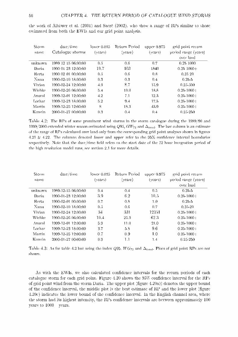
56 CHAPTER 4. THE RETURN PERIOD OF CATALOGUE WIND STORMS
the work of Albisser et al. (2001) and Sacré (2002), who show a range of RPs similar to thoseestimated from both the EWIs and our grid point analysis.
Storm date/time lower 0.025 Return Period upper 0.975 grid point return
name Catalogue storms (years) (years) (years) period range (years)
over land
unknown 1989-12-15 06:00:00 0.5 0.6 0.7 0.25-1000
Daria 1990-01-23 12:00:00 19.7 103 1840 0.25-1000+
Herta 1990-02-01 00:00:00 0.5 0.6 0.8 0.25-20
Nana 1990-02-10 18:00:00 0.3 0.3 0.4 0.25-5
Vivian 1990-02-24 12:00:00 4.9 8.7 15.9 0.25-500
Wiebke 1990-02-26 06:00:00 5.4 10.0 18.8 0.25-1000+
Anatol 1999-12-01 12:00:00 4.2 7.1 12.3 0.25-1000+
Lothar 1999-12-23 18:00:00 5.2 9.4 17.5 0.25-1000+
Martin 1999-12-25 12:00:00 8 18.3 43.9 0.25-1000+
Kerstin 2000-01-27 00:00:00 0.3 0.4 0.4 0.25-250
Table 4.2: The RPs of some prominent wind storms in the storm catalogue during the 1989/90 and
1999/2000 extended winter season estimated using Q95, GW72 and �land. The last column is an estimate
of the range of RPs calculated over land only from the corresponding grid point analyses shown in �gures
4.21 & 4.22. The columns denoted lower and upper refer to the 95% con�dence interval boundaries
respectively. Note that the date/time �eld refers to the start date of the 72 hour integration period of
the high resolution model runs, see section 2.1 for more details.
Storm date/time lower 0.025 Return Period upper 0.975 grid point return
name (years) (years) (years) period range (years)
over land
unknown 1989-12-15 06:00:00 0.4 0.4 0.5 0.25-5
Daria 1990-01-23 12:00:00 3.9 6.2 10.5 0.25-1000+
Herta 1990-02-01 00:00:00 0.7 0.8 1.0 0.25-5
Nana 1990-02-10 18:00:00 0.5 0.6 0.7 0.25-20
Vivian 1990-02-24 12:00:00 34 331 12351 0.25-1000+
Wiebke 1990-02-26 06:00:00 10.4 25.3 62.3 0.25-1000+
Anatol 1999-12-01 12:00:00 5.9 11.0 21.0 0.25-1000+
Lothar 1999-12-23 18:00:00 3.7 5.8 9.6 0.25-1000+
Martin 1999-12-25 12:00:00 0.7 0.9 1.0 0.25-1000+
Kerstin 2000-01-27 00:00:00 0.9 1.1 1.4 0.25-250
Table 4.3: As for table 4.2 but using the index Q95, WG72 and �land. Plots of grid point RPs are not
shown.
As with the EWIs, we also calculated con�dence intervals for the return periods of eachcatalogue storm for each grid point. Figure 4.20 shows the 95% con�dence interval for the RPsof grid point wind from the storm Daria. The upper plot (�gure 4.20a)) denotes the upper boundof the con�dence interval, the middle plot is the best estimate of RP and the lower plot (�gure4.20c) indicates the lower bound of the con�dence interval. In the English channel area, wherethe storm had its highest intensity, the RPs con�dence intervals are between approximately 100years to 1000+ years.
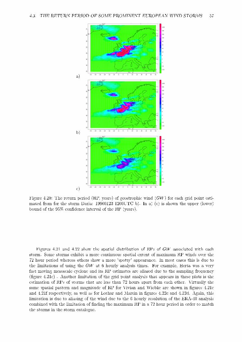
4.3. THE RETURN PERIOD OF SOME PROMINENT EUROPEAN WIND STORMS 57
a)
0.25
0.5
1
2
5
10
20
30
50
100
250
500
1000
GWS: GP Analysis for PRE_storms − 1990012312 − upper confidence interval (95%)
−35 −30 −25 −20 −15 −10 −5 0 5 10 15 20 25 30 35
3540
4550
5560
6570
b)
0.25
0.5
1
2
5
10
20
30
50
100
250
500
1000
GWS: GP Analysis for PRE_storms − 1990012312 − Return Period
−35 −30 −25 −20 −15 −10 −5 0 5 10 15 20 25 30 35
3540
4550
5560
6570
c)
0.25
0.5
1
2
5
10
20
30
50
100
250
500
1000
GWS: GP Analysis for PRE_storms − 1990012312 − lower confidence interval (95%)
−35 −30 −25 −20 −15 −10 −5 0 5 10 15 20 25 30 35
3540
4550
5560
6570
Figure 4.20: The return period (RP, years) of geostrophic wind (GW ) for each grid point esti-mated from for the storm Daria: 19900123 1200UTC b). In a) (c) is shown the upper (lower)bound of the 95% con�dence interval of the RP (years).
Figures 4.21 and 4.22 show the spatial distribution of RPs of GW associated with eachstorm. Some storms exhibit a more continuous spatial extent of maximum RP winds over the72 hour period whereas others show a more 'spotty' appearance. In most cases this is due tothe limitations of using the GW at 6 hourly analysis times. For example, Herta was a veryfast moving mesoscale cyclone and its RP estimates are aliased due to the sampling frequency(�gure 4.21c) . Another limitation of the grid point analysis that appears in these plots is theestimation of RPs of storms that are less than 72 hours apart from each other. Virtually thesame spatial pattern and magnitude of RP for Vivian and Wiebke are shown in �gures 4.21eand 4.21f respectively, as well as for Lothar and Martin in �gures 4.22c and 4.22d. Again, thislimitation is due to aliasing of the wind due to the 6 hourly resolution of the ERA-40 analysiscombined with the limitation of �nding the maximum RP in a 72 hour period in order to matchthe storms in the storm catalogue.

58 CHAPTER 4. THE RETURN PERIOD OF CATALOGUE WIND STORMS
0.25
0.5
1
2
5
10
20
30
50
100
250
500
1000
GWS: GP Analysis for PRE_storms − 1989121506 − Return Period
−35 −30 −25 −20 −15 −10 −5 0 5 10 15 20 25 30 35
3540
4550
5560
6570
a)
0.25
0.5
1
2
5
10
20
30
50
100
250
500
1000
GWS: GP Analysis for PRE_storms − 1989121506 − Return Period
−35 −30 −25 −20 −15 −10 −5 0 5 10 15 20 25 30 35
3540
4550
5560
6570
b)
0.25
0.5
1
2
5
10
20
30
50
100
250
500
1000
GWS: GP Analysis for PRE_storms − 1990012312 − Return Period
−35 −30 −25 −20 −15 −10 −5 0 5 10 15 20 25 30 35
3540
4550
5560
6570
c)
0.25
0.5
1
2
5
10
20
30
50
100
250
500
1000
GWS: GP Analysis for PRE_storms − 1990020100 − Return Period
−35 −30 −25 −20 −15 −10 −5 0 5 10 15 20 25 30 35
3540
4550
5560
6570
d)
0.25
0.5
1
2
5
10
20
30
50
100
250
500
1000
GWS: GP Analysis for PRE_storms − 1990021018 − Return Period
−35 −30 −25 −20 −15 −10 −5 0 5 10 15 20 25 30 3535
4045
5055
6065
70
e)
0.25
0.5
1
2
5
10
20
30
50
100
250
500
1000
GWS: GP Analysis for PRE_storms − 1990022412 − Return Period
−35 −30 −25 −20 −15 −10 −5 0 5 10 15 20 25 30 35
3540
4550
5560
6570
f)
0.25
0.5
1
2
5
10
20
30
50
100
250
500
1000
GWS: GP Analysis for PRE_storms − 1990022606 − Return Period
−35 −30 −25 −20 −15 −10 −5 0 5 10 15 20 25 30 35
3540
4550
5560
6570
Figure 4.21: The RP (years) for each grid point for each catalogue storm in the 1990/90 October- April extended winter season estimated from GW and using the EVA detailed in section 3.a) unknown name: 19891215 0600UTC, b) Daria: 19900123 1200UTC , c) Herta: 199002010000UTC, d) Nana: 19900210 1800UTC, e) Vivian: 19900224 1200UTC, f) Wiebke: 199002260600UTC. The RP scale is in the top left of the plot.

4.4. THE EVALUATIONOF THE EXTREMEWIND INDICESWITHGRID POINT STATISTICS59
0.25
0.5
1
2
5
10
20
30
50
100
250
500
1000
GWS: GP Analysis for PRE_storms − 1989121506 − Return Period
−35 −30 −25 −20 −15 −10 −5 0 5 10 15 20 25 30 35
3540
4550
5560
6570
a)
0.25
0.5
1
2
5
10
20
30
50
100
250
500
1000
GWS: GP Analysis for PRE_storms − 1999120112 − Return Period
−35 −30 −25 −20 −15 −10 −5 0 5 10 15 20 25 30 35
3540
4550
5560
6570
b)
0.25
0.5
1
2
5
10
20
30
50
100
250
500
1000
GWS: GP Analysis for PRE_storms − 1999122318 − Return Period
−35 −30 −25 −20 −15 −10 −5 0 5 10 15 20 25 30 35
3540
4550
5560
6570
c)
0.25
0.5
1
2
5
10
20
30
50
100
250
500
1000
GWS: GP Analysis for PRE_storms − 1999122512 − Return Period
−35 −30 −25 −20 −15 −10 −5 0 5 10 15 20 25 30 35
3540
4550
5560
6570
d)
0.25
0.5
1
2
5
10
20
30
50
100
250
500
1000
GWS: GP Analysis for PRE_storms − 2000012700 − Return Period
−35 −30 −25 −20 −15 −10 −5 0 5 10 15 20 25 30 3535
4045
5055
6065
70
Figure 4.22: The RP (years) for each grid point for each catalogue storm in the 1999/2000October - April extended winter season estimated from GW and using the EVA detailed insection 3. a) Anatol: 19991201 1200UTC, b) Lothar: 19991223 1800UTC , c) Martin: 199912251200UTC, d) Kerstin: 20000127 1800UTC. The RP scale is in the top left of the plot.
4.4 The evaluation of the extreme wind indices with grid point
statistics
A basic evaluation of the ability of the EWI RP estimates to represent the grid point wind basedRP estimates for the 96 wind storms has been performed using a Spearman rank correlationanalysis. Both �gures 4.23a and 4.24a show that the rank of the RPs of Q95 and �X EWI aremost highly correlated with the rank of the RPs from the grid point analysis over a regioncentered in the middle western part of the domain over the North Atlantic Ocean with r valuesin the order of 0.6. However, the rank correlation decreases radially from this point such that rover the European coast and further inland is less than about 0.25 implying that these indicescan only explain 6% or less variability of the local grid point RPs. Results are better if weonly consider EWI using land only grid points. Here, again we see a 'bullseye' (�gures 4.23band 4.24b) centered on western Europe roughly in the center of the land domain. Within theseregions r range from 0.0 to 0.7 indicating that up to 50% of RP variations at the grid point levelcan be explained by the EWI.

60 CHAPTER 4. THE RETURN PERIOD OF CATALOGUE WIND STORMS
a)
0
0.1
0.15
0.2
0.25
0.3
0.35
0.4
0.45
0.5
0.6
0.7
0.8
0.9
EvaluationRP Storms: wQ95 vs. gp−values, all_gp Cor Method: Spearman
−35 −30 −25 −20 −15 −10 −5 0 5 10 15 20 25 30 35
3540
4550
5560
6570
b)
0
0.1
0.15
0.2
0.25
0.3
0.35
0.4
0.45
0.5
0.6
0.7
0.8
0.9
EvaluationRP Storms: wQ95 vs. gp−values, land_only Cor Method: Spearman
−35 −30 −25 −20 −15 −10 −5 0 5 10 15 20 25 30 35
3540
4550
5560
6570
Figure 4.23: The Spearman rank correlation between the return periods of the 96 cataloguestorms based on Q95 of GW72 and the return period at each grid point based on GW , a) over�all , and b) �land.
a)
0
0.1
0.15
0.2
0.25
0.3
0.35
0.4
0.45
0.5
0.6
0.7
0.8
0.9
EvaluationRP Storms: wMean vs. gp−values, all_gp Cor Method: Spearman
−35 −30 −25 −20 −15 −10 −5 0 5 10 15 20 25 30 35
3540
4550
5560
6570
b)
0
0.1
0.15
0.2
0.25
0.3
0.35
0.4
0.45
0.5
0.6
0.7
0.8
0.9
EvaluationRP Storms: wMean vs. gp−values, land_only Cor Method: Spearman
−35 −30 −25 −20 −15 −10 −5 0 5 10 15 20 25 30 35
3540
4550
5560
6570
Figure 4.24: The Spearman rank correlation between the return periods of the 96 cataloguestorms based on �X of GW72 and the return period at each grid point based on GW , a) over �all
, and b) �land.
4.5 Discussion of results
Our results show that estimating the RPs of known wind storm events is subject to manyuncertainties. Firstly there is uncertainty associated with the statistical model used to describethe extreme value distribution (section 3.3), secondly there are uncertainties associated with thetype of analysis performed, either using a spatial summary statistic (EWI) or individual gridpoint wind, and thirdly, but not least, is the e�ect of using di�erent data on which to calculatethese estimates.
ERA-40 derived geostrophic wind at 850hPa does not exhibit unrealistic spatial and tempo-ral characteristics, as wind gust does over areas of complex orography, although we note thatthere seems to be higher magnitude winds over the Alps. We believe the �ow (850hPa level)is accelerated by the smooth model orography, therefore in this area we would consider the RPestimates to be less reliable (when considering its usefulness as an indicator of surface winds) .The overall increased reliability of using geostrophic wind speed in areas of complex orography iso�set to a certain extent by the aliasing e�ects of using 6 hourly analysis times, whereas the windgust �eld is the maximum wind gust within a 6 hour period of the reanalysis. This is evident insome results from the grid point analysis.
We used the pro�le log-likelihood method to obtain uncertainty estimates of the RPs andshowed that it gave more realistic structures to the RP uncertainty estimates than two other

4.5. DISCUSSION OF RESULTS 61
commonly used approaches.
A possible shortcoming of our method of storm selection is that it is based on a statisticaldeclustering method and therefore does not contain information about the dynamical situationwhich may help identi�cation of storm events. Other methods of storm selection, for example,Lagrangian identi�cation techniques for cyclones are also subject to many uncertainties (Raibleet al., 2007). A possible alternative to the storm selection process can be found in recent literaturewhich suggests that when using the GPD it may be possible to avoid declustering the POTseries by altering the statistics used to make statistical inferences on the parameters (Fawcettand Walshaw, 2006a,b).
From the results of the EWIs it is clear that some indices performed more consistently thanothers (section 4.1 and table 4.1). The indices �X, Sfq95, Sfq95q99 have the highest inter-indexand inter-dataset RP correlations, however Q95 has a higher spread in RP of catalogue storms.SQ95 should not be considered further as an suitable EWI, it consistently underestimates theRP of catalogue storms in comparison with other EWIs due to the low variability of this index.The best correlations between RPs based on the same index using di�erent data (inter-dataset)are generally lower than the best inter-index correlations indicating that the dataset plays animportant role in the calculation of the RPs. A possible explanation for these di�erences is themasking that is applied to WG72 and WG, however, we demonstrate that this has a relativelyminor e�ect on RP di�erences. We suggest that the main cause of RP di�erences based on EWIsis a) the restrictive nature of the any spatial summary index which is not equally sensitive to alltypes of wind storm wind �elds and b) due to fundamental di�erences between the WG72 andGW72 datasets. For example, the known biases in using geostrophic wind in the free atmosphereto infer severity of wind extremes at the surface (Miller, 2003). Wind gust on the other hand isa highly parameterised model forecast �eld and is unrealistic in areas of complex orography. Amajor di�erence between the datasets is that GW72 is based on the 6 hourly analysis whereasWG72 is a maximum over a 6 hour period. As we can see in the grid point analysis this has ledto some aliasing of the extreme wind signal. Another aspect of the data which prevented a moreaccurate RP estimate for catalogue storms that are very close to each other in time is the 72hour maximum wind calculation (section 2.2). This aspect of the data processing prevents theestimates of RPs from storms such as Lothar and Martin from being independent. It was notedthat in many cases the catalogue storms did not match the cluster maxima of the EWI exactly.This could be due to the fact that the catalogue storm dates were chosen to simulate the timeperiod when the storm had the highest impacts on PartnerRe assets and not necessarily whenthe storm had its highest intensity. In some cases a cluster maxima of the POT series indicatedthat a storm occurred but did not appear as a storm in the catalogue. Again, this is due to thedi�erent sampling strategy of the catalogue storms (aimed at highest impacts) and the limitednumber of storms able to be simulated at high resolution.
The grid point analysis produces qualitatively very similar spatial patterns of RP estimatesusing either GW or WG (where not masked). The grid point analysis often shows areas withmuch higher RPs than the RPs calculated from EWIs. This is obviously due to the e�ect ofspatial averaging. The basic evaluation of the ability of EWIs based RP estimates to explain theRP estimates at the grid point indicate that between 0 and 50% of the grid point RP variabilitycan be explained over continental Europe. The EWIs are sensitive to speci�c areas of the domain,compounding the problem of comparing RP estimates with the grid point approach. We see thisas a limitation of the EWI approach, if one of the intended purposes of these indices is to tryand explain local loss �gures. However, we also show that the RP of catalogue storms at the gridpoint level is also very sensitive to the choice of wind data used. We believe that this is partlydue to the aliasing problems of GW but also due to the fact that during our data processing wehave interpolated the grid to 0.5� which is roughly half of the original resolution of the ERA-40data, therefore we may be seeing sensitivity (added sampling noise) to the interpolation processat the grid point level. Better agreement might be possible using a slightly larger area averageRP. When we consider that one of the fundamental questions of this study was to obtain a better

62 CHAPTER 4. THE RETURN PERIOD OF CATALOGUE WIND STORMS
estimate of the frequency of a wind storm, then, given our current understanding of the problem,the EWIs o�er the most valuable information. At the same time we should keep in mind thatthe EWI RP estimates are highly dependent on the domain chosen and as such they representa storm which could of occurred anywhere over the domain (from a statistical point of view).Hence, the RP of Daria calculated using an EWI should be expressed as the RP of a storm of
Daria's magnitude to a�ect any part of the domain. Whereas the grid point analysis answersthe question what is the RP of the local wind caused by Daria?

Chapter 5
Conclusions and Recommendations for
Further Research
5.1 Conclusions
MeteoSwiss have used state of the art reanalysis data combined with innovative extreme valueanalysis techniques to the problem of estimating the recurrence frequency of the high resolutionwind storms of the PartnerRe storm catalogue. Our analysis techniques have focused only onobtaining the return period of these events, since the ERA-40 reanalysis dataset has biasesassociated with the magnitude of wind and wind gusts. We have shown that the generalisedPareto distribution is a robust extreme value model of the declustered peak over thresholdseries. The POT series was obtained using a sophisticated automatic declustering method whichlargely avoided the need for the speci�cation of arbitrary parameters such is the case with morecommon declustering methods. We have used one of the most accurate methods in the literatureto determine the uncertainty of the catalogue storm return periods.
The wind gust �eld of ERA-40 should be treated with extreme caution in areas where theroughness length parameter is high (> 3m), due to the boundary layer physics in the ERA-40model. We recommend using derived geostrophic wind from the ERA-40 geopotential height�eld as an alternative to wind gust (although model u and v winds may also give good results)for determining the return periods of storms which a�ected areas where wind gust was masked.
We have tried to answer the question 'what is the return period of a particular storm event?'through the use of extreme wind indices and a grid point based approach. Neither method iscompletely satisfactory at answering this question. The EWIs are a spatial summary statistic andhence the return periods estimates are more representative of the return period of a storm, thatcould of occurred anywhere over the chosen domain, compared with the RP estimates derivedfrom the grid point approach. In section 4 it was demonstrated that return period estimates foreach storm, based on di�erent indices and di�erent base datasets in many cases varied by morethan the uncertainty estimates calculated from the GPD �t. Results showed that the extremewind indices could explain up to 50% of variations in grid point based RP estimates. The largerthe domain considered the lower the e�ectiveness of the EWI at explaining local wind RPs. TheEWI RP estimates were generally much lower than the grid point RP estimates. We concludethat it is very di�cult to obtain a spatial summary statistic (EWI) which works equally well foreach type of storm event in the context of trying to estimate a storm RP. On the other hand, thelocal wind grid point RPs also show dependency between datasets, due to aliasing problems andwe may not be able to e�ectively estimate the return period of the storm given that no spatialdependence between grid point RPs has been modelled.
In conclusion, the results of the project demonstrate that signi�cant progress has been madethrough the development of an extreme wind climatology based on a robust reanalysis dataset.We have created a climatology of wind storm RPs based on EWIs together with estimates oftheir local wind RP using the grid point approach. There remain considerable challenges both
63

from the methodological treatment of spatial extreme events and from the limitations imposedby the currently available datasets. We look forward to continuing our research to address thesetwo issues.
5.2 Recommendations for further research
As more accurate and longer datasets of either in-situ wind data or pressure datasets becomeavailable (Diaz et al., 2002; Alexander et al., 2005; Ansell et al., 2006) this analysis should berepeated in order to minimise the uncertainty in the return period calculations. Another possiblesource of data which is starting to become more accessible to the climate community are ERA-40dynamically downscaled regional climate simulations (e.g. the ENSEMBLES project). Use ofthis data should allow inferences about the wind gust magnitude to be made as well as a moreaccurate spatial assessment of the wind gust return periods (Heneka et al., 2006; Leckebuschet al., 2006, 2007; Schwierz et al., 2007). It is evident that there are some storms identi�edin ERA-40 which are not included in the storm catalogue that, both the EWI EVA and thegrid point EVA have identi�ed as being extreme. Further investigation of these storms eitherusing ERA-40 or the RCM output of ENSEMBLES project could be used as a basis for addingmore historical events to the storm catalogue. We also recommend further research into thespatial structure of historical wind storm events through the application of advanced spatialEVA techniques (Coles, 2001). Promising applications of Bayesian spatial extreme methods canbe found in the work of Cooley et al. (2006, 2007). One should also consider using approachesthat do not require the declustering of data prior to creating a POT series (Fawcett and Walshaw,2006a,b). More research is also needed on determining the predictability of these events, eitheron weather or seasonal timescales (Chang et al., 2002; Wernli et al., 2002; Yan et al., 2002; Junget al., 2005, 2006; Walser et al., 2006). Given the lack of longer and more reliable reanalysisor in-situ data, utilisation of the ever increasing amount of dynamical ensemble prediction data(van den Brink, Konnen and Opsteegh, 2004; van den Brink, Konnen, Opsteegh, van Oldenborghand Burgers, 2004; Jung et al., 2005; Frei et al., 2006) is suggested as a means to build morerealistic estimates of the frequency of wind storms.
64

65

66

Acknowledgements
We wish to acknowledge the reinsurance company PartnerRe who substantially sponsored thisresearch. We wish to thank Jan Kleinn, Hervé Castella, Malcolm Haylock and Manuel Prechtlof PartnerRe for useful discussions and input to this research report. Paul Della-Marta waspartially sponsored by the 6th EU framework program ENSEMBLES contract number GOCE-CT-2003-505539 and by the Swiss National Science Foundation through the National Centrefor Competence in Research Climate (NCCR-Climate). The majority of the computing wasperformed using R statistical software.
67

68

Bibliography
Ahrens, J. H. and Dieter, U.: 1982, Computer generation of poisson deviates from modi�ednormal distributions, ACM Transactions on Mathematical Software 8, 163�179.
Albisser, P., Aller, D., Bader, S., Brnag, P., Broccard, A., Bründl, A., Dobbertin, M., Forster, B.,Frutig, F., Hächler, P., Hänggli, T., Jacobi, C., Müller, E., Neu, U., Niemeyer, S., Nöthiger,C. J., Quiby, J., Rickli, C., Schilling, A., Schibiger, F. and Truog, G.: 2001, Lothar Der Orkan1999, Eidg. Forchungsanstalt WSL, Bundesamt für Umwelt, Wald und Landschaft BUWAL,Birmensdorf, Bern.
Alexander, L. V., Tett, S. F. B. and Jonsson, T.: 2005, Recent observed changes in severe stormsover the united kingdom and iceland, Geophysical Research Letters 32(13), L13704.
Alexandersson, H. ., Schmith, T., Iden, K. and Tuomenvirta, H.: 1998, Long-term variations ofthe storm climate over nw europe., Global Atmospheric and Ocean Systems 6, 97�120.
Alexandersson, H., Tuomenvirta, H., Schmith, T. and Iden, K.: 2000, Trends of storms in nweurope derived from an updated pressure data set, Climate Research 14(1), 71�73.
Ansell, T. J., Jones, P. D., Allan, R. J., Lister, D., Parker, D. E., Brunet, M., Moberg, A.,Jacobeit, J., Brohan, P., Rayner, N. A., Aguilar, E., Alexandersson, H., Barriendos, M.,Brandsma, T., Cox, N. J., Della-Marta, P. M., Drebs, A., Founda, D., Gerstengarbe, F.,Hickey, K., Jonsson, T., Luterbacher, J., Nordli, O., Oesterle, H., Petrakis, M., Philipp, A.,Rodwell, M. J., Saladie, O., Sigro, J., Slonosky, V., Srnec, L., Swail, V., Garcia-Suarez, A. M.,Tuomenvirta, H., Wang, X., Wanner, H., Werner, P., Wheeler, D. and Xoplaki, E.: 2006, Dailymean sea level pressure reconstructions for the european-north atlantic region for the period1850-2003, Journal Of Climate 19(12), 2717�2742.
Appenzeller, C., Stocker, T. F. and Anklin, M.: 1998, North atlantic oscillation dynamicsrecorded in greenland ice cores, Science 282(5388), 446�449.
Barring, L. and von Storch, H.: 2004, Scandinavian storminess since about 1800, GeophysicalResearch Letters 31(20), L20202.
Beersma, J. J., Rider, K. M., Komen, G. J., Kaas, E. and Kharin, V. V.: 1997, An analysisof extra-tropical storms in the north atlantic region as simulated in a control and 2xco(2)time-slice experiment with a high-resolution atmospheric model, Tellus Series A-Dynamic
Meteorology And Oceanography 49(3), 347�361.
Bengtsson, L., Hagemann, S. and Hodges, K. I.: 2004, Can climate trends be calculated fromreanalysis data?, Journal Of Geophysical Research-Atmospheres 109(D11), D11111.
Bengtsson, L., Hodges, K. I. and Roeckner, E.: 2006, Storm tracks and climate change, JournalOf Climate 19(15), 3518�3543.
Bhend, J.: 2005, North atlantic and european cyclones: Their variability and change from 1881
to 2003, Master's thesis, Institute of Geography, University of Berne, Switzerland.
69

Bijl, W., Flather, R., de Ronde, J. G. and Schmith, T.: 1999, Changing storminess? an analysisof long-term sea level data sets, Climate Research 11(2), 161�172.
Bouette, J. C., Chassagneux, J. F., Sibai, D., Terron, R. and Charpentier, A.: 2006, Windin ireland: long memory or seasonal e�ect?, Stochastic Environmental Research And Risk
Assessment 20(3), 141�151.
Brabson, B. B. and Palutikof, J. P.: 2000, Tests of the generalized pareto distribution for pre-dicting extreme wind speeds, Journal Of Applied Meteorology 39(9), 1627�1640.
Caires, S. and Sterl, A.: 2005, 100-year return value estimates for ocean wind speed and signi�-cant wave height from the era-40 data, Journal Of Climate 18(7), 1032�1048.
Carretero, J. C., Gomez, M., Lozano, I., de Elvira, A. R., Serrano, O., Iden, K., Reistad, M.,Reichardt, H., Kharin, V., Stolley, M., von Storch, H., Gunther, H., P�zenmayer, A., Rosethal,W., Stawarz, M., Schmith, T., Kaas, E., Li, T., Alexandersson, H., Beersma, J., Bouws, E.,Komen, G., Rider, K., Flather, R., Smith, J., Bijl, W., de Ronde, J., Mietus, M., Bauer, E.,Schmidt, H. and Langenberg, H.: 1998, Changing waves and storms in the northeast atlantic?,Bulletin Of The American Meteorological Society 79(5), 741�760.
Chang, E. K. M., Lee, S. Y. and Swanson, K. L.: 2002, Storm track dynamics, Journal OfClimate 15(16), 2163�2183.
Coles, S.: 2001, An introduction to statistical modeling of extreme values, Springer.
Cooley, D., Naveau, P., Jomelli, V., Rabatel, A. and Grancher, D.: 2006, A bayesian hierarchicalextreme value model for lichenometry, Environmetrics 17(6), 555�574.
Cooley, D., Nychka, D. and Naveau, P.: 2007, Bayesian spatial modeling of extreme precipitationreturn levels, Journal of the American Statistical Association .
Diaz, H., Folland, C., Manabe, T., Parker, D., Reynolds, R. and Woodru�, S.: 2002, Workshopon advances in the use of historical marine climate data, CLIVAR Exchanges 25, 71�73.
Dukes, M. D. G. and Palutikof, J. P.: 1995, Estimation of extreme wind speeds with very longreturn periods, Journal Of Applied Meteorology 34(9), 1950�1961.
Fawcett, L. and Walshaw, D.: 2006a, A hierarchical model for extreme wind speeds, Journal OfThe Royal Statistical Society Series C-Applied Statistics 55, 631�646.
Fawcett, L. and Walshaw, D.: 2006b, Markov chain models for extreme wind speeds, Environ-metrics 17(8), 795�809.
Ferro, C. A. T. and Segers, J.: 2003, Inference for clusters of extreme values, Journal Of TheRoyal Statistical Society Series B-Statistical Methodology 65, 545�556.
Fisher, R. A. and Tippett, L. H. C.: 1928, Limiting forms of the frequency distribution of thelargest or smallest member of a sample, Proceedings Of The Cambridge Philosophical Society
24, 180�190.
Frei, C., Scholl, R., Fukutome, S., Schmidli, R. and Vidale, P. L.: 2006, Future change ofprecipitation extremes in europe: Intercomparison of scenarios from regional climate models,Journal Of Geophysical Research-Atmospheres 111(D6), D06105.
Gillett, N. P., Allan, R. J. and Ansell, T. J.: 2005, Detection of external in�uence on sea levelpressure with a multi-model ensemble, Geophysical Research Letters 32(19), L19714.
Gillett, N. P., Zwiers, F. W., Weaver, A. J. and Stott, P. A.: 2003, Detection of human in�uenceon sea-level pressure, Nature 422(6929), 292�294.
70
Graybeal, D. Y.: 2006, Relationships among daily mean and maximum wind speeds, with appli-cation to data quality assurance, International Journal Of Climatology 26(1), 29�43.
Held, I. M.: 1993, Large-scale dynamics and global warming, Bulletin Of The American Meteo-
rological Society 74(2), 228�241.
Heneka, P., Hofherr, T., Ruck, B. and Kottmeier, C.: 2006, Winter storm risk of residentialstructures-model development and application to the german state of baden-wurttemberg,Natural Hazards And Earth System Sciences 6(5), 721�733.
Holton, J. R.: 2004, An introduction to Dynamic Meteorology, Elsevier.
Horvitz, D. G. and Thompson, D. J.: 1952, A generalization of sampling without replacementfrom a �nite universe, Journal of the American Statistical Association 47, 663�685.
Hurrel, J. W., Kushnir, Y., Ottersen, G. and Visbeck, M.: 2002, The North Atlantic Oscilla-
tion: Climatic Signi�cance and Environmental Impact Geophysical Monograph 134, AmericanGeophysical Union, Washington, DC, chapter An Overview of the North Atlantic Oscillation,pp. 1�36.
Jones, P. D., Horton, E. B., Folland, C. K., Hulme, M., Parker, D. E. and Basnett, T. A.: 1999,The use of indices to identify changes in climatic extremes, Climatic Change 42(1), 131�149.
Jung, T., Gulev, S. K., Rudeva, I. and Soloviov, V.: 2006, Sensitivity of extratropical cyclonecharacteristics to horizontal resolution in the ecmwf model, Quarterly Journal Of The Royal
Meteorological Society 132(619), 1839�1857.
Jung, T., Klinker, E. and Uppala, S.: 2005, Reanalysis and reforecast of three major europeanstorms of the twentieth century using the ecmwf forecasting system. part ii: Ensemble forecasts,Meteorological Applications 12(2), 111�122.
Kaas, E., Li, T. S. and Schmith, T.: 1996, Statistical hindcast of wind climatology in the northatlantic and northwestern european region, Climate Research 7, 97�110.
Kalnay, E., Kanamitsu, M., Kistler, R., Collins, W., Deaven, D., Gandin, L., Iredell, M., Saha,S., White, G., Woollen, J., Zhu, Y., Chelliah, M., Ebisuzaki, W., Higgins, W., Janowiak,J., Mo, K., Ropelewski, C., Wang, J., Leetmaa, A., Reynolds, R., Jenne, R. and Joseph,D.: 1996, The ncep/ncar 40-year reanalysis project, Bulletin of the American Meteorological
Society 77, 437�471.
Kasperski, M.: 2002, A new wind zone map of germany, Journal Of Wind Engineering And
Industrial Aerodynamics 90(11), 1271�1287.
Knippertz, P., Ulbrich, U. and Speth, P.: 2000, Changing cyclones and surface wind speeds overthe north atlantic and europe in a transient ghg experiment, Climate Research 15(2), 109�122.
Kristensen, L., Rathmann, O. and Hansen, S. O.: 1999, Extreme winds in denmark, Technicalreport, Riso National Laboratory.
Kunz, H., Scherrer, S. C., Liniger, M. A. and Appenzeller, C.: 2007, The evolution of era-40surface temperatures and total ozone compared to observed swiss time series, Meteorologische
Zeitschrift 16, 171�181.
Lamb, H. H.: 1991, Historic Storms of the North Sea, British Isles, and Northwest Europe,Cambridge University Press.
Leckebusch, G. C., Ko�, B., Ulbrich, U., Pinto, J. G., Spangehl, T. and Zacharias, S.: 2006,Analysis of frequency and intensity of european winter storm events from a multi-model per-spective, at synoptic and regional scales, Climate Research 31(1), 59�74.
71
Leckebusch, G. C., Ulbrich, U., Frohlich, L. and Pinto, J. G.: 2007, Property loss poten-tials for european midlatitude storms in a changing climate, Geophysical Research Letters
34(5), L05703.
Luterbacher, J., Xoplaki, E., Dietrich, D., Rickli, R., Jacobeit, J., Beck, C., Gyalistras, D.,Schmutz, C. and Wanner, H.: 2002, Reconstruction of sea level pressure �elds over the easternnorth atlantic and europe back to 1500, Climate Dynamics 18(7), 545�561.
Mailier, P. J., Stephenson, D. B., Ferro, C. A. T. and Hodges, K. I.: 2006, Serial clustering ofextratropical cyclones, Monthly Weather Review 134(8), 2224�2240.
Martins, E. S. and Stedinger, J. R.: 2000, Generalized maximum-likelihood generalized extreme-value quantile estimators for hydrologic data, Water Resources Research 36(3), 737�744.
Miller, C.: 2003, A once in 50-year wind speed map for europe derived from mean sea levelpressure measurements, Journal Of Wind Engineering And Industrial Aerodynamics 91(12-15), 1813�1826.
Monahan, A. H.: 2004, A simple model for the skewness of global sea surface winds, Journal OfThe Atmospheric Sciences 61(16), 2037�2049.
Monahan, A. H.: 2006, The probability distribution of sea surface wind speeds. part 1: Theoryand seawinds observations, Journal Of Climate 19(4), 497�520.
Morland, J., Deuber, B., Feist, D. G., Martin, L., Nyeki, S., Kampfer, N., Matzler, C., Jeannet, P.and Vuilleumier, L.: 2006, The startwave atmospheric water database, Atmospheric ChemistryAnd Physics 6, 2039�2056.
Palutikof, J. P., Brabson, B. B., Lister, D. H. and Adcock, S. T.: 1999, A review of methods tocalculate extreme wind speeds, Meteorological Applications 6(2), 119�132.
Philipp, A., Della-Marta, P. M., Jacobeit, J., Fereday, D. R., Jones, P. D., Moberg, A. andWanner, H.: 2006, Long term variability of daily north atlantic�european pressure patternssince 1850 classi�ed by simulated annealing clustering, Journal of Climate 20(16), 4065�4095.
Pinto, J. G., Spangehl, T., Ulbrich, U. and Speth, P.: 2006, Assessment of winter cyclone activityin a transient echam4-opyc3 ghg experiment, Meteorologische Zeitschrift 15(3), 279�291.
Pinto, J. G., Ulbrich, U., Leckebusch, G. C., Spangehl, T., Reyers, M. and Zacharias, S.: 2007,Changes in storm track and cyclone activity in three sres ensemble experiments with theecham5/mpi-om1 gcm, Climate Dynamics 29(2-3), 195�210.
Pryor, S. C. and Barthelmie, R. J.: 2003, Long-term trends in near-surface �ow over the baltic,International Journal Of Climatology 23(3), 271�289.
Pryor, S. C., Schoof, J. T. and Barthelmie, R. J.: 2006, Winds of change?: Projections of near-surface winds under climate change scenarios, Geophysical Research Letters 33(11), L11702.
Raible, C. C.: 2007, On the relation between extremes of midlatitude cyclones and the atmo-spheric circulation using era40, Geophysical Research Letters 34(7), L07703.
Raible, C. C., Della-Marta, P. M., Schwierz, C., Wernli, H. and Blender, R.: 2007, Northernhemisphere midlatitude cyclones: A comparison of detection and tracking methods and di�er-ent reanalyses, Monthly Weather Review In Press.
Research Triangle Institute: 2001, Sudaan user's manual, release 8.0, Technical report, ResearchTriangle Park, NC: Research Triangle Institute.
72

Rockel, B. and Woth, K.: 2007, Future changes in near surface wind speed extremes over europefrom an ensemble of rcm simulations, Climate Change .
Sacré, C.: 2002, Extreme wind speed in france: the '99 storms and their consequences, JournalOf Wind Engineering And Industrial Aerodynamics 90(10), 1163�1171.
Schiesser, H. H., P�ster, C. and Bader, J.: 1997, Winter storms in switzerland north of the alps1864/1865-1993/1994, Theoretical And Applied Climatology 58(1-2), 1�19.
Schinke, H.: 1993, On the occurence of deep cyclones over europe and the north atlantic in theperiod 1930-1991., Beiträge zur Physik der Atmosphäre 66, 223�237.
Schmith, T., Kaas, E. and Li, T. S.: 1998, Northeast atlantic winter storminess 1875-1995 re-analysed, Climate Dynamics 14, 529�536.
Schubiger, F., Lopez, S., Turina, A. and Romaneessen, E.: 2004, Re-analyse von extremenwetterereignissen mit dem lm ausgehend aus dem ecmwf era-40 datensatz, DACH.
Schwierz, C., Heck, P., Zenklusen, E., Bresch, D. N., Vidale, P., M., W. and Schär, C.: 2007,Modelling European winter wind storm losses in current and future climate, Climatic ChangeSubmitted, 1�35.
Seierstad, I. A., Stephenson, D. B. and Kvamsto, N. G.: 2007, How useful are teleconnectionpatterns for explaining variability in extratropical storminess ?, Tellus Series A-Dynamic Me-
teorology And Oceanography 59(2), 170�181.
Smits, A., Tank, A. M. G. K. and Konnen, G. P.: 2005, Trends in storminess over the netherlands,1962-2002, International Journal Of Climatology 25(10), 1331�1344.
Sterl, A.: 2004, On the (in)homogeneity of reanalysis products, Journal Of Climate 17(19), 3866�3873.
Turina, A., Lopez, S., Schubiger, F., Aichinger, M. and Romaneessen, E.: 2004, High-resolutionre-analysis of extreme weather events - part a: The hazard model, Geophysical Research Ab-
stracts, Vol. 6, 01236, 2004.
Uppala, S. M., Kallberg, P. W., Simmons, A. J., Andrae, U., Bechtold, V. D., Fiorino, M.,Gibson, J. K., Haseler, J., Hernandez, A., Kelly, G. A., Li, X., Onogi, K., Saarinen, S., Sokka,N., Allan, R. P., Andersson, E., Arpe, K., Balmaseda, M. A., Beljaars, A. C. M., Van De Berg,L., Bidlot, J., Bormann, N., Caires, S., Chevallier, F., Dethof, A., Dragosavac, M., Fisher, M.,Fuentes, M., Hagemann, S., Holm, E., Hoskins, B. J., Isaksen, L., Janssen, P. A. E. M., Jenne,R., McNally, A. P., Mahfouf, J. F., Morcrette, J. J., Rayner, N. A., Saunders, R. W., Simon,P., Sterl, A., Trenberth, K. E., Untch, A., Vasiljevic, D., Viterbo, P. and Woollen, J.: 2005,The era-40 re-analysis, Quarterly Journal Of The Royal Meteorological Society 131(612), 2961�3012.
van den Brink, H. W., Konnen, G. P. and Opsteegh, J. D.: 2004, Statistics of extreme synoptic-scale wind speeds in ensemble simulations of current and future climate, Journal Of Climate17(23), 4564�4574.
van den Brink, H. W., Konnen, G. P., Opsteegh, J. D., van Oldenborgh, G. J. and Burgers, G.:2004, Improving 10(4)-year surge level estimates using data of the ecmwf seasonal predictionsystem, Geophysical Research Letters 31(17), L17210.
Verkaik, J. W.: 2000, Evaluation of two gustiness models for exposure correction calculations,Journal Of Applied Meteorology 39(9), 1613�1626.
73
Walser, A., Arpagaus, M., Appenzeller, C. and Leutbecher, M.: 2006, The impact of moistsingular vectors and horizontal resolution on short-range limited-area ensemble forecasts fortwo european winter storms, Monthly Weather Review 134(10), 2877�2887.
Walter, A., Keuler, K., Jacob, D., Knoche, R., Block, A., Kotlarski, S., Muller-Westermeier, G.,Rechid, D. and Ahrens, W.: 2006, A high resolution reference data set of german wind velocity1951-2001 and comparison with regional climate model results, Meteorologische Zeitschrift
15(6), 585�596.
Wanner, H., Bronnimann, S., Casty, C., Gyalistras, D., Luterbacher, J., Schmutz, C., Stephen-son, D. and Xoplaki, E.: 2001, North atlantic oscillation - concepts and studies, Surveys in
Geophysics 22, 321�382.
Weisse, R., Von Storch, H. and Feser, F.: 2005, Northeast atlantic and north sea storminess assimulated by a regional climate model during 1958-2001 and comparison with observations,Journal Of Climate 18(3), 465�479.
Wernli, H., Dirren, S., Liniger, M. A. and Zillig, M.: 2002, Dynamical aspects of the life cycle ofthe winter storm 'lothar' (24-26 december 1999), Quarterly Journal Of The Royal Meteorolog-
ical Society 128(580), 405�429.
White, P.: 2003, IFS documentation cycle cy23r41, part iv: Physical processes, Technical report,European Center for Medium Range Forecasting.
Yan, Z., Bate, S., Chandler, R. E., Isham, V. and Wheater, H.: 2006, Changes in extremewind speeds in nw europe simulated by generalized linear models, Theoretical And Applied
Climatology 83(1-4), 121�137.
Yan, Z. W., Bate, S., Chandler, R. E., Isham, V. and Wheater, H.: 2002, An analysis of dailymaximum wind speed in northwestern europe using generalized linear models, Journal OfClimate 15(15), 2073�2088.
Yin, J. H.: 2005, A consistent poleward shift of the storm tracks in simulations of 21st centuryclimate, Geophysical Research Letters 32(18), L18701.
74

Kürzlich erschienen
Arbeitsberichte der MeteoSchweiz 215 Begert M, Seiz G, Foppa N, Schlegel T, Appenzeller C, Müller G: 2007, Die Überführung der
klimatologischen Referenzstationen der Schweiz in das Swiss National Climatological Network (Swiss NBCN), 47 pp., CHF 68.-
214 Schmucki D., Weigel A., 2006, Saisonale Vorhersage in Tradition und Moderne: Vergleich der "Sommerprognose" des Zürcher Bööggs mit einem dynamischen Klimamodell, 46pp, CHF 68.-
213 Frei C: 2006, Eine Länder übergreifende Niederschlagsanalyse zum August Hochwasser 2005. Ergänzung zu Arbeitsbericht 211, 10pp, CHF 59.-
212 Z’graggen, L: 2006, Die Maximaltemperaturen im Hitzesommer 2003 und Vergleich zu früheren Extremtemperaturen, 74pp, CHF 75.-
211 MeteoSchweiz: 2006, Starkniederschlagsereignis August 2005, 63pp., CHF 72.-
210 Buss S, Jäger E and Schmutz C: 2005: Evaluation of turbulence forecasts with the aLMo, 58pp, CHF 70.–
209 Schmutz C, Schmuki D, Duding O, Rohling S: 2004, Aeronautical Climatological Information Sion LSGS, 77pp, CHF 25.–
208 Schmuki D, Schmutz C, Rohling S: 2004, Aeronautical Climatological Information Grenchen LSZG, 73pp, CHF 24.–
207 Moesch M, Zelenka A: 2004, Globalstrahlungsmessungen 1981-2000 im ANETZ, 83pp, CHF 26.–
206 Schmutz C, Schmuki D, Rohling S: 2004, Aeronautical Climatological Information St.Gallen LSZR, 78pp, CHF 25.–
205 Schmutz C, Schmuki D, Ambrosetti P, Gaia M, Rohling S: 2004, Aeronautical Climatological Information Lugano LSZA, 81pp, CHF 26.–
204 Schmuki D, Schmutz C, Rohling S: 2004, Aeronautical Climatological Information Bern LSZB, 80pp, CHF 25.–
203 Duding O, Schmuki D, Schmutz C, Rohling S: 2004, Aeronautical Climatological Information Geneva LSGG, 104pp, CHF 31.–
202 Bader S: 2004, Tropische Wirbelstürme – Hurricanes –Typhoons – Cyclones, 40pp, CHF 16.-
201 Schmutz C, Schmuki D, Rohling S: 2004, Aeronautical Climatological Information Zurich LSZH, 110pp, CHF 34.-
200 Bader S: 2004, Die extreme Sommerhitze im aussergewöhnlichen Witterungsjahr 2003, 25pp, CHF 14.-
199 Frei T, Dössegger R, Galli G, Ruffieux D: 2002, Konzept Messsysteme 2010 von MeteoSchweiz, 100pp, CHF 32.-
198 Kaufmann P: 2002, Swiss Model Simulations for Extreme Rainfall Events on the South Side of the Alps, 40pp, CHF 20.-
197 WRC Davos (Ed): 2001, IPC - IX, 25.9. - 13.10.2000, Davos, Switzerland, 100pp, CHF 32.-
196 Hächler P et al.: 1999, Der Föhnfall vom April 1993, 139pp, CHF 40.-
195 Urfer Ch, Vogt R, 1999, Die Niederschlagsverhältnisse in Basel 1964-1998, 43pp, CHF 40.-
194 Courvoisier HW: 1998, Statistik der 24-stündigen Starkniederschläge in der Schweiz 1901-1996, 20pp, CHF 11.-
193 Defila C, Vonderach G: 1998, Todesfälle und Wetterlagen in Schaffhausen, 72pp, CHF 25.-
Frühere Veröffentlichungen und Arbeitsberichte finden sich unter www.meteoschweiz.ch » Forschung » Publikationen

Veröffentlichungen der MeteoSchweiz 77 Rossa AM: 2007, MAP-NWS – an Optional EUMETNET Programme in Support of an Optimal Research
Programme, Veröffentlichung MeteoSchweiz, 77, 67 pp., CHF 73.- 76 Baggenstos D: 2007, Probabilistic verification of operational monthly temperature forecasts,
Veröffentlichung MeteoSchweiz, 76, 52 pp.,CHF 69.-
75 Fikke S, Ronsten G, Heimo A, Kunz S, Ostrozlik M, Persson PE, Sabata J, Wareing B, Wichura B, Chum J, Laakso T, Säntti K, Makkonen L: 2007, COST 727: Atmospheric Icing on Structures Measurements and data collection on icing: State of the Art, 110pp, CHF 83.-
74 Schmutz C, Müller P, Barodte B: 2006, Potenzialabklärung für Public Private Partnership (PPP) bei MeteoSchweiz und armasuisse Immobilien, 82pp, CHF 76.-
73 Scherrer SC: 2006, Interannual climate variability in the European and Alpine region, 132pp, CHF 86.-
72 Mathis H: 2005, Impact of Realistic Greenhouse Gas Forcing on Seasonal Forecast Performance, 80pp, CHF 75.
71 Leuenberger D: 2005, High-Resolution Radar Rainfall Assimilation: Exploratory Studies with Latent Heat Nudging, 103pp, CHF 81.-
70 Müller G und Viatte P: 2005, The Swiss Contribution to the Global Atmosphere Watch Programme – Achievements of the First Decade and Future Prospects, 112pp, CHF 83.-
69 Müller WA: 2004, Analysis and Prediction of the European Winter Climate, 115pp, CHF 34.
68 Bader S: 2004, Das Schweizer Klima im Trend: Temperatur- und Niederschlagsentwicklung seit 1864, 48pp, CHF 18.-
67 Begert M, Seiz G, Schlegel T, Musa M, Baudraz G und Moesch M: 2003, Homogenisierung von Klimamessreihen der Schweiz und Bestimmung der Normwerte 1961-1990, Schluss-bericht des Projektes NORM90, 170pp, CHF 40.-
66 Schär Christoph, Binder Peter, Richner Hans (Eds.): 2003, International Conference on Alpine Meteorology and MAP Meeting 2003, Extended Abstracts volumes A and B, 580pp, CHF 100.
65 Stübi R: 2002, SONDEX / OZEX campaigns of dual ozone sondes flights: Report on the data analysis, 78pp, CHF 27.-
64 Bolliger M: 2002, On the characteristics of heavy precipitation systems observed by Meteosat-6 during the MAP-SOP, 116pp, CHF 36.-
63 Favaro G, Jeannet P, Stübi R: 2002, Re-evaluation and trend analysis of the Payerne ozone sounding, 99pp, CHF 33.-
62 Bettems JM: 2001, EUCOS impact study using the limited-area non-hydrostatic NWP model in operational use at MeteoSwiss, 17pp, CHF 12.-
61 Richner H, et al.: 1999, Grundlagen aerologischer Messungen speziell mittels der Schweizer Sonde SRS 400, 140pp, CHF 42.-
60 Gisler O: 1999, Zu r Methodik einer Beschreibung der Entwicklung des linearen Trends der Lufttemperatur über der Schweiz im Zeitabschnitt von 1864 bis 1990, 125pp, CHF 36.-
59 Bettems J-M: 1999, The impact of hypothetical wind profiler networks on numerical weather prediction in the Alpine region, 65pp, CHF 25.-
58 Baudenbacher, M: 1997, Homogenisierung langer Klimareihen, dargelegt am Beispiel der Lufttemperatur, 181pp, CHF 50.-
57 Bosshard, W: 1996, Homogenisierung klimatologischer Zeitreihen, dargelegt am Beispiel der relativen Sonnenscheindauer, 136pp, CHF 38.-