Extreme Precipitation in an Atmosphere General Circulation Model:Impact of Horizontal and Vertical Model Resolutions

CLAUDIA VOLOSCIUK AND DOUGLAS MARAUN

GEOMAR Helmholtz Centre for Ocean Research Kiel, Kiel, Germany

VLADIMIR A. SEMENOV

GEOMAR Helmholtz Centre for Ocean Research Kiel, Kiel, Germany, and A. M. Obukhov Institute of

Atmospheric Physics, and P. P. Shirshov Institute of Oceanology, and Institute of Geography,

Russian Academy of Sciences, Moscow, Russia

WONSUN PARK

GEOMAR Helmholtz Centre for Ocean Research Kiel, Kiel, Germany

(Manuscript received 9 May 2014, in final form 27 October 2014)

ABSTRACT

To investigate the influence of atmospheric model resolution on the representation of daily precipitation

extremes, ensemble simulations with the atmospheric general circulation model ECHAM5 at different hori-

zontal (from T213 to T31 spectral truncation) and vertical (from L31 to L19) resolutions and forced with ob-

served sea surface temperatures and sea ice concentrations have been carried out for January 1982–September

2010.All results have been comparedwith the highest resolution, which has been validated against observations.

Resolution affects both the representation of physical processes and the averaging of precipitation across

grid boxes. The latter, in particular, smooths out localized extreme events. These effects have been disen-

tangled by averaging precipitation simulated at the highest resolution to the corresponding coarser grid.

Extremes are represented by seasonal maxima, modeled by the generalized extreme value distribution.

Effects of averaging and representation of physical processes vary with region and season. In the tropical

summer hemisphere, extreme precipitation is reduced by up to 30% due to the averaging effect, and a further

65% owing to a coarser representation of physical processes. Toward middle to high latitudes, the latter effect

reduces to 20%; in the winter hemisphere it vanishes toward the poles. A strong drop is found betweenT106 and

T63 in the convection-dominated tropics. At the lowest resolution, Northern Hemisphere winter precipitation

extremes, mainly caused by large-scale weather systems, are in general represented reasonably well. Coarser

vertical resolution causes an equatorward shift of maximum extreme precipitation in the tropics. The impact of

vertical resolution on mean precipitation is less pronounced; for horizontal resolution it is negligible.

1. Introduction

Much of our knowledge about future changes in ex-

treme weather events and the mechanisms causing these

changes is based on global climatemodel simulations that

employ general circulation models (GCMs). There is

confidence that climate models provide credible quanti-

tative estimates of future climate change, particularly at

larger scales, because of their physical basis and the

ability of models to reproduce observed climate and past

climate changes (Flato et al. 2013). The representation of

mean precipitation patterns has steadily improved be-

tween each phase of the CoupledModel Intercomparison

Project (CMIP) used for the Intergovernmental Panel on

Climate Change (IPCC) assessment reports (Flato et al.

2013). However, confidence in projections of extremes is

generally weaker than for projections of long-term aver-

ages (Seneviratne et al. 2012). Extreme precipitation in-

tensities (e.g., Sun et al. 2006), frequencies (e.g., Allan

and Soden 2008), and return levels (Wehner et al. 2010)

are generally underestimated by GCMs.

The simulation of precipitation is muchmore complex

than that of temperature; anisotropic multifractal

Corresponding author address: Claudia Volosciuk, GEOMAR

Helmholtz Centre for Ocean Research Kiel, Duesternbrooker

Weg 20, 24105 Kiel, Germany.

E-mail: cvolosciuk@geomar.de

1184 JOURNAL OF CL IMATE VOLUME 28

DOI: 10.1175/JCLI-D-14-00337.1

� 2015 American Meteorological Society

behavior over a wide range of scales has been attributed

to precipitation (e.g., Lovejoy and Schertzer 1995) and

the simulation of precipitation depends heavily on pro-

cesses that are parameterized in current GCMs (Flato

et al. 2013). To accurately represent extreme pre-

cipitation, models must correctly simulate atmospheric

humidity as well as a number of relevant processes, such

as evapotranspiration, condensation, and transport

processes (Randall et al. 2007). There are uncertainties

in the simulation of the water cycle in most GCMs from

phase 3 of CMIP (CMIP3) due to a time-varying im-

balanced atmospheric moisture budget. These biases in

turn imply biases in the energy balance (Liepert and

Previdi 2012; Lucarini and Ragone 2011).

Along with the increase of computational capacity

since the First Assessment Report (FAR) of the IPCC,

typical model resolution for short-term climate simula-

tions has increased from T21 (;500 km) in the FAR to

T106 (;110 km) in the Fourth Assessment Report

(AR4) (Le Treut et al. 2007). Vertical resolution has

also increased, from 10 atmospheric layers in the FAR to

about 30 layers in the AR4 (Le Treut et al. 2007).

Nevertheless, resolving all important spatial and tem-

poral scales remains beyond current capabilities for

transient global climate change simulations (Le Treut

et al. 2007). Biases thus remain, particularly on smaller

scales and in the tropics, where the regional distribution

of precipitation is strongly determined by convection, on

a wide range of spatial and temporal scales, and on in-

teractions between convective processes and the large-

scale circulation (Flato et al. 2013). For high-resolution

projections of precipitation extremes, different ap-

proaches have been employed: high-resolution GCMs,

dynamical downscaling using regional climate models

(RCMs) (Rummukainen 2010), and statistical down-

scaling (Maraun et al. 2010).

Several studies have investigated the resolution de-

pendence of spatial precipitation patterns in atmo-

spheric general circulation models (AGCMs). For

example, patterns of seasonal mean precipitation in the

NCAR Community Climate Model version 3 (CCM3;

Duffy et al. 2003; Iorio et al. 2004), as well as patterns of

extreme precipitation (20-yr return levels) in the

NCAR finite volume dynamical core version of CAM2

(fvCAM2; Wehner et al. 2010), are better represented

over the United States with enhanced model resolution.

Wehner et al. (2010) suggest 0.58 3 0.6258, their highestresolution, to be a breakthrough resolution for the

representation of extreme precipitation. However,

precipitation intensity is still limited at this resolution,

particularly for tropical cyclones (Wehner et al. 2010).

Kopparla et al. (2013) have found biases in high per-

centiles (.95th) of daily precipitation in the NCAR

CAM4 to decrease with finer resolution over the United

States andEurope, whereas their highest resolution (0.258)overestimates these high percentiles over Australia. Li

et al. (2011) have shown in aquaplanet simulationswith the

CAM3 model that total precipitation increases at higher

resolutions, especially in the tropics. The larger scales of

the zonal average precipitation converge with increasing

resolution for T85 and higher in the aquaplanet version of

CAM3 (Williamson 2008). Seasonal differences in re-

solution dependence of extreme precipitation are in-

dicated by Prein et al. (2013), who have found different

mechanisms to be responsible for the higher-resolution

requirement in June–August (JJA) (more small-scale

convective events) than in December–February (DJF) in

an RCM over the Colorado headwaters.

Changing horizontal model resolution has two effects

on the representation of precipitation, in particular on

its extremes. First, GCM-simulated precipitation rep-

resents gridbox area averages (e.g., Osborn and Hulme

1997; Chen and Knutson 2008); the coarser the model

resolution, the more strongly localized events are

smoothed out. To account for this ‘‘averaging effect,’’

Chen and Knutson (2008) advise comparing extreme

rainfall for different model resolutions after all data

have been averaged to the lowest considered model

resolution. Second, coarser model resolution involves

reduced precision in the simulation of various features,

especially feedbacks from smaller to larger scales. These

feedbacks, including the impact of changes in resolved

scales as well as in subgrid scales represented by pa-

rameterizations, deteriorate with coarser resolution.

Hence, we refer to this effect as the ‘‘scale interaction

effect.’’ For instance, transient vertical velocities, and

accordingly vertical moisture transport, are simulated

more accurately with enhanced horizontal resolution

(Pope and Stratton 2002; Li et al. 2011). A better rep-

resentation of orography, due to higher horizontal res-

olution, improves local precipitation patterns (e.g.,

Smith et al. 2013; Pope and Stratton 2002; Duffy et al.

2003; Iorio et al. 2004) and has remote effects on the

storm tracks as well as on the mean circulation (Pope

and Stratton 2002; Jung et al. 2006). In general, changes

in resolution mostly affect resolved scales, but there are

also impacts on the parameterized physics (Roeckner

et al. 2004). The more realistic representation of re-

solved dynamical properties provides, in turn, improved

input to the parameterization schemes. Also, the in-

teraction between parameterization schemes (e.g., be-

tween the convection and cloud microphysics schemes)

is more detailed at higher resolution. Finally, truncation

causes artificial separation of resolved and unresolved

(i.e., parameterized) processes (Arakawa 2004). When

changing the horizontal model resolution, one faces the

1 FEBRUARY 2015 VOLOSC IUK ET AL . 1185

combined effects of averaging and scale interaction. We

call these overall effects ‘‘resolution effects.’’1

Changing vertical resolution affects several physical

processes, particularly those related to the hydrological

cycle. Higher vertical resolution leads to a marked re-

distribution of humidity and clouds (Roeckner et al.

2006). Most notable is the drying of the upper tropo-

sphere, which is related to a lowering of the tropopause

and hygropause (Roeckner et al. 2006). In the tropics,

the response of humidity and clouds to increased vertical

resolution is related to changes in cloud top detrainment

of water vapor and cloud water/ice (Roeckner et al.

2006). These improvements are largely due to the

smaller numerical diffusion at higher vertical resolution,

allowing for a larger, and also more realistic, vertical

moisture gradient to be maintained throughout the

troposphere (Hagemann et al. 2006). These changes in

humidity and clouds in turn influence precipitation. On

the global scale, both precipitation and evaporation are

smaller at higher vertical resolution over land, in better

agreement with observations (Hagemann et al. 2006).

Finally, the sensitivity of the hydrological cycle to ver-

tical resolution might be closely related to the tropo-

spheric moisture changes caused by a more accurate

vertical moisture transport at higher vertical resolution

(Hagemann et al. 2006).

Which minimum resolution of GCMs is sufficient to

represent patterns and characteristics of extreme pre-

cipitation at the global scale remains an open question.

To our knowledge, there is no study investigating the

resolution dependence of extreme precipitation on the

global scale, with realistic topography, and separately

for different seasons. We are also not aware of any study

investigating the impact of vertical resolution on ex-

treme precipitation. While it is widely acknowledged

that the averaging effect plays an important role when

evaluating extreme precipitation on gridded datasets,

and therefore should be removed before any compari-

sons of extreme precipitation from different sources are

carried out, its separation from the overall resolution

effect and quantification across different scales remains

an open question.

Here, we study the dependency of extreme pre-

cipitation on horizontal and vertical model resolution.

In particular, we address the following questions:

1) What is the importance of the averaging effect to the

overall resolution effect when simulating extreme

precipitation?

2) To what extent does representation of extreme pre-

cipitation at different resolutions depend on season?

3) At which resolution, compared with the highest con-

sidered resolution, is the strongest deterioration in the

representation of extreme precipitation evident?

4) Are there regions where the dependence of extreme

precipitation on resolution is weak or where the scale

interaction effect can be neglected?

5) What is the influence of vertical resolution on the

representation of extreme precipitation?

In section 2 of the paper, we describe the setup of the

atmospheric model, the design of the resolution exper-

iment, and the statistical model used to analyze ex-

tremes. In section 3, modeled extreme precipitation

return levels at different horizontal and vertical resolu-

tions are compared for different seasons. Finally, section 4

contains the conclusions.

2. Data and methods

We consider daily precipitation simulated by the

ECHAM5 AGCM. A key part of our study is to disen-

tangle the averaging and scale interaction effects. To this

end, we consider simulations at different resolutions and

compare them with the highest-resolution simulation,

averaged to the corresponding lower spatial scales as

recommended by Chen and Knutson (2008).

a. The atmospheric general circulation model

We use the ECHAM5AGCM (Roeckner et al. 2003),

developed at the Max Planck Institute for Meteorology,

Germany. ECHAM5 is a global spectral model and

calculates precipitation fluxes on the Gaussian trans-

form grid (Roeckner et al. 2003). The sensitivity of

ECHAM5 to horizontal and vertical resolution has been

studied for mean climate characteristics (Roeckner et al.

2006) and the hydrological cycle (Hagemann et al.

2006). Notable deficiencies in the hydrological cycle are

a dry bias over Australia and a lack of a rain forest cli-

mate in central Africa, where precipitation is too low

during the dry season (Hagemann et al. 2006). The

ECHAM5 model overestimates precipitation over the

oceans, especially in high-resolution simulations. This

bias is a general problem in current GCMs that could

possibly be related to insufficient atmospheric absorp-

tion of solar radiation by aerosols, water vapor, or clouds

(Hagemann et al. 2006). The bias of basic climate vari-

ables decreases monotonically with increasing horizon-

tal resolution from T42 to T159 spectral truncation

(Roeckner et al. 2006).

As the 31-level (L31) vertical resolution versions are

superior to their L19 counterparts, except for T42

1Note that resolution effects include changing grid size as well

as changing the resolution dependent tunable parameters; see

section 2b.

1186 JOURNAL OF CL IMATE VOLUME 28

horizontal resolution, Roeckner et al. (2006) recom-

mend the vertical resolution L19 for the horizontal

resolutions T31 and T42, and the vertical resolution L31

for higher horizontal resolutions. Enhanced vertical

resolution is more beneficial than increased horizontal

resolution for the simulation of mean precipitation in

ECHAM5 (Hagemann et al. 2006).

b. Experiments

We carried out simulations covering the period Jan-

uary 1982–September 2010 (29 yr), driven with the same

transient present-day boundary forcing for all resolu-

tions. Sea surface temperatures (SSTs) and sea ice

concentrations (SICs) were interpolated to the cor-

responding horizontal resolutions from daily 1/48 opti-

mal interpolation SST analysis (OISST), version 2,

(Reynolds et al. 2007) and high-resolution (12.7 km)

observed SIC from Grumbine (1996) of the National

Oceanic and Atmospheric Administration (NOAA).

Greenhouse gas forcing was kept constant at present-

day concentrations (348 ppm). An overview of the dif-

ferent horizontal and vertical resolutions of these

simulations is given in Table 1. Three ensemble re-

alizations of the resolutions T106L31, T63L31, T42L19,

and T31L19 were run to assess internal variability. The

top four and bottom two vertical levels of L31 and L19

are similar. The greatest difference (doubling) in verti-

cal resolution occurs between approximately 70 and

500 hPa (Roeckner et al. 2003). In all resolutions we

used the default ECHAM5 parameterization and the

parameter settings recommended by Roeckner et al.

(2004, 2006) for the respective resolution. Note that our

aim is not to isolate the sensitivity of the dynamical and

physical response to pure grid spacing from the sensi-

tivity of modeled precipitation to tunable parameters.

Such intention would require experiments with fixed

parameterizations and tuning parameter values such as

proposed in Leung et al. (2013) and applied by, for ex-

ample, Rauscher et al. (2013). Our objective is rather to

quantify the effect of changing themodel resolution, and

to separate this effect into the contribution of spatial

averaging and the residual scale interaction effect. Our

definitions of both scale interaction and resolution effect

thus are not limited to changing the grid spacing, but

additionally include the adaptation of tunable parame-

ters to recommended values, as feedback from param-

eterizations also interactwith different scales.Nevertheless,

additional experiments showed that the sensitivity of ex-

treme precipitation to parameter choice is negligible in the

range of considered resolutions (not shown).

c. Statistical model

We modeled daily precipitation extremes with the

block maxima approach, following the Fisher–Tippet

theorem: Given a sequence of n independent identically

distributed random variablesXi, i5 1, . . . , n, the properly

rescaled maximum of this sequence Mn converges for

large n—in case a limiting distribution exists—to the

generalized extreme value (GEV) family of distributions

(Fisher and Tippett 1928; Gnedenko 1943; Coles 2001):

G(z)5 expn2h11 j

�z2m

s

�i21/jo, (1)

with the location parameter m, the scale parameter s,

and the shape parameter j. The tail of the distribution is

determined by j as follows: j / 0: infinite smooth tail;

j . 0: infinite heavy tail; and j , 0: bounded tail (Coles

2001). The independence assumption of the Fisher–

Tippet theorem can be relaxed to a wide class of sta-

tionary, but not necessarily independent, processes

(Coles 2001; Rust 2009; Faranda et al. 2011, 2013).

Extreme quantiles are obtained by inverting Eq. (1):

zp 5

8<:

m2s

jf12 [2log(12 p)]2jg for j 6¼ 0

m2s log[2log(12 p)] for j5 0

, (2)

whereG(zp)5 12 p. The return level zp associated with

the return period 1/p is expected to be exceeded on

average once in 1/p blocks; that is, zp is exceeded in any

particular block with probability p (Coles 2001).

Parameters of the GEV distribution [Eq. (1)] were

estimated with probability weighted moments (PWM)

(Hosking et al. 1985) using the ‘‘fExtremes’’ package

(Wuertz et al. 2009) in R (R Development Core Team

2011). PWM performs well for small sample sizes and is

computational efficient (Hosking et al. 1985). The

analysis was carried out seasonally. A block length of

one season (i.e., three months) turned out to be a good

compromise between an appropriate fit for most regions

and a sufficiently long maxima time series of 29 yr to

keep sampling uncertainties reasonably low. To avoid

a misfit of the GEV distribution in very dry regions, we

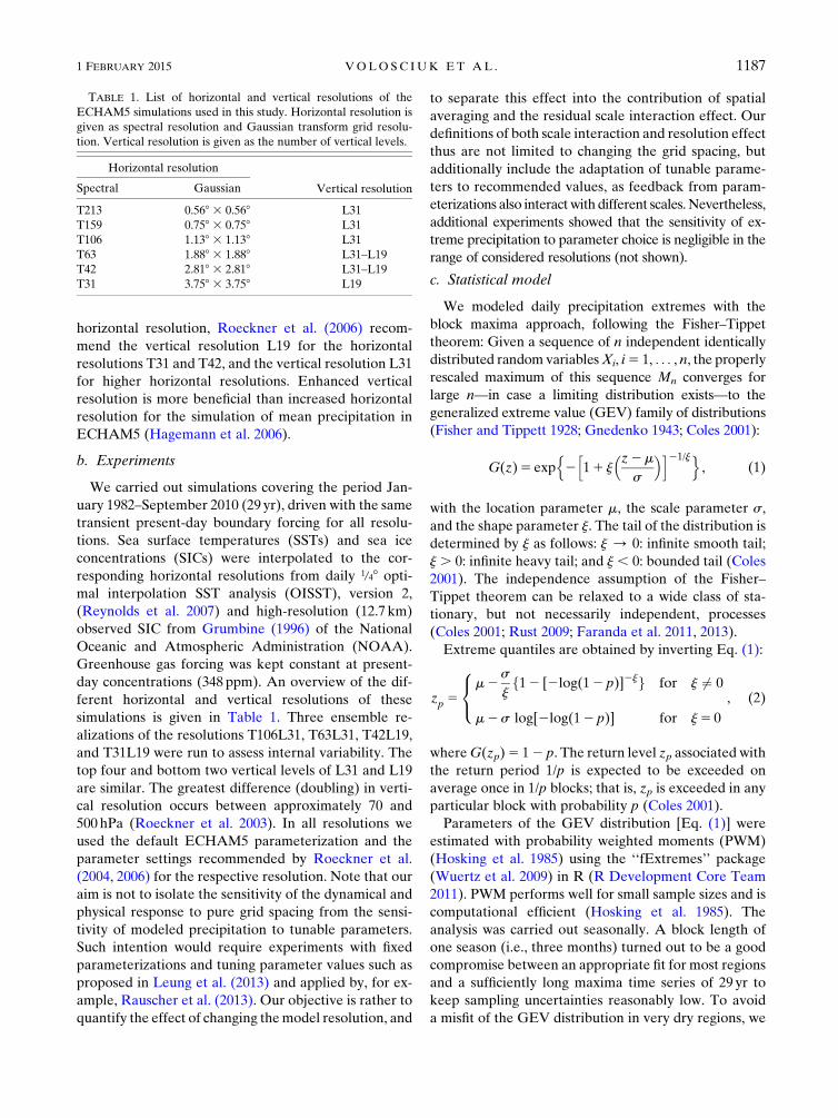
TABLE 1. List of horizontal and vertical resolutions of the

ECHAM5 simulations used in this study. Horizontal resolution is

given as spectral resolution and Gaussian transform grid resolu-

tion. Vertical resolution is given as the number of vertical levels.

Horizontal resolution

Vertical resolutionSpectral Gaussian

T213 0.568 3 0.568 L31

T159 0.758 3 0.758 L31

T106 1.138 3 1.138 L31

T63 1.888 3 1.888 L31–L19

T42 2.818 3 2.818 L31–L19

T31 3.758 3 3.758 L19

1 FEBRUARY 2015 VOLOSC IUK ET AL . 1187

excluded time series from our analysis that contained

more than one zero in the seasonal maxima time series.

As a representation of extreme events, we considered

the 20-season return level of daily precipitation

(RL20S). For example, the RL20S for DJF is exceeded

in any DJF season with the probability 1/20 (i.e., on av-

erage every 20th DJF season). The RL20S is already

reasonably extreme, but still low enough to avoid biases

caused by the estimation procedure (Hosking et al.

1985) or undesirably high estimation uncertainty. Sam-

pling uncertainties of RL20S were assessed by a boot-

strap method (see appendix for details).

d. Separation of averaging and scale interactioneffects

The results of the simulations at different model reso-

lutions are compared with our highest resolution

(T213L31). Chen and Knutson (2008) advise that, when

comparing extreme precipitation from different sources,

precipitation should be averaged to the same spatial scale

beforehand, as climatemodels provide gridbox averages of

precipitation [e.g., Roeckner et al. (2003) for ECHAM5],

which includes the averaging effect if precipitation is

compared on different grids. We averaged daily pre-

cipitation at the highest horizontal resolution (T213) to

coarser grids for comparison with the coarser resolutions

on similar spatial scales (see Table 2). Statistics were cal-

culated after daily precipitation had been averaged to the

appropriate spatial scale. In the following, we refer to the

simulations carried out at different model resolutions

(Table 1) as coarser-resolution simulations (CRS). The

averagedT213 resolutions T213232, . . . , T213737 (Table 2)

are referred to as averaged high-resolution simulations

(AHS). The averaging effect was approximately disen-

tangled from the scale interaction effect by comparing

RL20S in CRSwith those in AHS on similar spatial scales.

3. Results and discussion

The highest resolution, T213L31, has been validated

against observational datasets: globally for seasonal

mean precipitation and over the United States, Europe,

Russia, theMiddle East, and Southeast Asia for extreme

precipitation. The global pattern of seasonal mean pre-

cipitation, as well as many features of the regional spa-

tial distribution of RL20S, is well represented (see

appendix for details).

a. Resolution and averaging effect

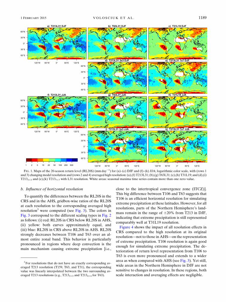
Figure 1 illustrates the global pattern of RL20S as

a function of resolution for DJF and JJA. The first and

third rows (Figs. 1a–c and 1f–h) showCRSand, hence, the

full resolution effect, including both averaging and scale

interaction. The second and fourth rows (Figs. 1d,e,i,k)

showAHSand, thus, represent solely the averaging effect

in relation to the respective left panels (Figs. 1a,f). The

differences between the first (third) and second (fourth)

rows illustrate the scale interaction effect. The middle

panels differ in horizontal resolution, while the right

panels differ in horizontal and vertical resolution. The

general global pattern of the RL20S is captured by all

resolutions: differences are rather small and mainly re-

lated to reduced magnitudes.2 The differences between

RL20S in CRS and in AHS are in general smaller for

T63L31 than for T31L19 (see, e.g., the South Pacific in

DJF and Siberia in JJA). These differences indicate

a better performance of T63L31 in both DJF and JJA.

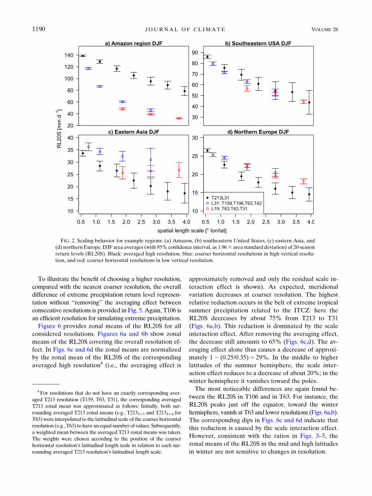
Figure 2 demonstrates the different effects for four ex-

ample regions: the tropical Amazon region, which is gov-

erned by deep convection; the southeasternUnited States,

a subtropical climate with mild winters; eastern Asia,

a continental climate with cold snowy winters; and

northern Europe, where winter precipitation is mainly

caused by large-scale weather systems. AHS (black) rep-

resents the averaging effect of RL20S (i.e., this scaling

dependence is caused by increased grid size). CRS (blue)

shows the overall resolution effects of the RL20S. The

difference between the RL20S in AHS and in CRS is

a first-order estimate of the scale interaction effect. The

pure averaging effect in general causes a decrease of

RL20S in AHS with increasing spatial length scale. The

same holds for CRS. Three different horizontal scaling

dependencies of RL20S are found. CRS can be below

(e.g., Amazon region), approximately equal to (95%

confidence intervals overlap; e.g., southeastern United

States), or above (e.g., eastern Asia) AHS. This finding

indicates that the dominantmechanism strongly influences

the scaling behavior and thereby also determines the

minimal required horizontal resolution. Different vertical

resolutions (blue and red) are compared in section 3c.

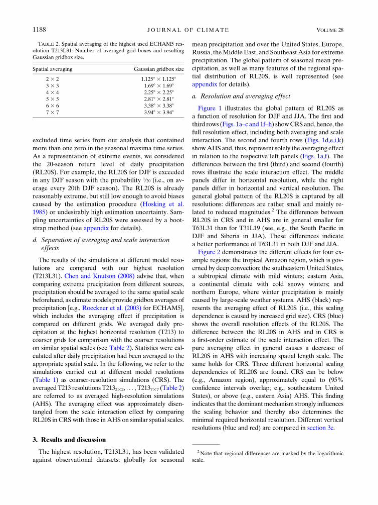
TABLE 2. Spatial averaging of the highest used ECHAM5 res-

olution T213L31: Number of averaged grid boxes and resulting

Gaussian gridbox size.

Spatial averaging Gaussian gridbox size

2 3 2 1.1258 3 1.12583 3 3 1.698 3 1.6984 3 4 2.258 3 2.2585 3 5 2.818 3 2.8186 3 6 3.388 3 3.3887 3 7 3.948 3 3.948

2Note that regional differences are masked by the logarithmic

scale.

1188 JOURNAL OF CL IMATE VOLUME 28

b. Influence of horizontal resolution

To quantify the differences between the RL20S in the

CRS and in the AHS, gridbox-wise ratios of the RL20S

at each resolution to the corresponding averaged high

resolution3 were computed (see Fig. 3). The colors in

Fig. 3 correspond to the different scaling types in Fig. 2

as follows: (i) red: RL20S in CRS below RL20S in AHS,

(ii) yellow: both curves approximately equal, and

(iii) blue: RL20S in CRS above RL20S in AHS. RL20S

strongly decreases between T106 and T63 over an al-

most entire zonal band. This behavior is particularly

pronounced in regions where deep convection is the

main mechanism causing extreme precipitation [i.e.,

close to the intertropical convergence zone (ITCZ)].

This big difference between T106 and T63 suggests that

T106 is an efficient horizontal resolution for simulating

extreme precipitation at these latitudes. However, for all

resolutions, parts of the Northern Hemisphere’s land-

mass remain in the range of 620% from T213 in DJF,

indicating that extreme precipitation is still represented

comparably well at T31L19 resolution.

Figure 4 shows the impact of all resolution effects in

CRS compared to the high resolution at its original

resolution—not to those inAHS—on the representation

of extreme precipitation. T106 resolution is again good

enough for simulating extreme precipitation. The de-

terioration of return level representation from T106 to

T63 is even more pronounced and extends to a wider

area as when compared with AHS (see Fig. 3). Yet still,

wide areas in the Northern Hemisphere in DJF are not

sensitive to changes in resolution. In these regions, both

scale interaction and averaging effects are negligible.

FIG. 1. Maps of the 20-season return level (RL20S) (mmday21) for (a)–(e) DJF and (f)–(k) JJA; logarithmic color scale, with (rows 1

and 3) changingmodel resolution and (rows 2 and 4) averaged high resolution: (a),(f) T213L31; (b),(g) T63L31; (c),(h) T31L19; and (d),(i)

T213333 and (e),(k) T213737 with L31 resolution. White areas: seasonal maxima time series contain more than one zero value.

3 For resolutions that do not have an exactly corresponding av-

eraged T213 resolution (T159, T63, and T31), the corresponding

value was linearly interpolated between the two surrounding av-

eraged T213 resolutions (e.g., T213333 and T213434 for T63).

1 FEBRUARY 2015 VOLOSC IUK ET AL . 1189

To illustrate the benefit of choosing a higher resolution,

compared with the nearest coarser resolution, the overall

difference of extreme precipitation return level represen-

tation without ‘‘removing’’ the averaging effect between

consecutive resolutions is provided in Fig. 5. Again, T106 is

an efficient resolution for simulating extreme precipitation.

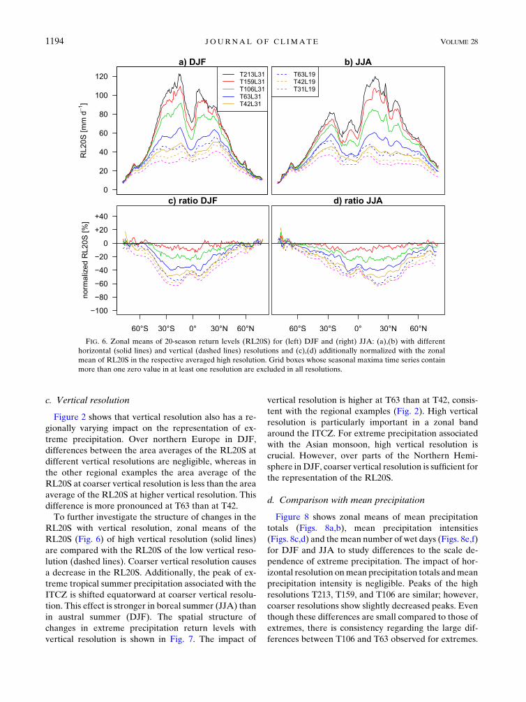
Figure 6 provides zonal means of the RL20S for all

considered resolutions. Figures 6a and 6b show zonal

means of the RL20S covering the overall resolution ef-

fect. In Figs. 6c and 6d the zonal means are normalized

by the zonal mean of the RL20S of the corresponding

averaged high resolution4 (i.e., the averaging effect is

approximately removed and only the residual scale in-

teraction effect is shown). As expected, meridional

variation decreases at coarser resolution. The highest

relative reduction occurs in the belt of extreme tropical

summer precipitation related to the ITCZ: here the

RL20S decreases by about 75% from T213 to T31

(Figs. 6a,b). This reduction is dominated by the scale

interaction effect. After removing the averaging effect,

the decrease still amounts to 65% (Figs. 6c,d). The av-

eraging effect alone thus causes a decrease of approxi-

mately 12 (0:25/0:35)5 29%. In the middle to higher

latitudes of the summer hemisphere, the scale inter-

action effect reduces to a decrease of about 20%; in the

winter hemisphere it vanishes toward the poles.

The most noticeable differences are again found be-

tween the RL20S in T106 and in T63. For instance, the

RL20S peaks just off the equator, toward the winter

hemisphere, vanish at T63 and lower resolutions (Figs. 6a,b).

The corresponding dips in Figs. 6c and 6d indicate that

this reduction is caused by the scale interaction effect.

However, consistent with the ratios in Figs. 3–5, the

zonal means of the RL20S in the mid and high latitudes

in winter are not sensitive to changes in resolution.

FIG. 2. Scaling behavior for example regions: (a) Amazon, (b) southeastern United States, (c) eastern Asia, and

(d) northernEurope.DJF area averages (with 95% confidence interval, as 1.963 area standard deviation) of 20-season

return levels (RL20S). Black: averaged high resolution, blue: coarser horizontal resolutions in high vertical resolu-

tion, and red: coarser horizontal resolutions in low vertical resolution.

4 For resolutions that do not have an exactly corresponding aver-

aged T213 resolution (T159, T63, T31), the corresponding averaged

T213 zonal mean was approximated as follows: Initially, both sur-

rounding averaged T213 zonal means (e.g., T213333 and T213434 for

T63)were interpolated to the latitudinal scale of the coarser horizontal

resolution (e.g., T63) to have an equal number of values. Subsequently,

a weighted mean between the averaged T213 zonal means was taken.

The weights were chosen according to the position of the coarser

horizontal resolution’s latitudinal length scale in relation to each sur-

rounding averaged T213 resolution’s latitudinal length scale.

1190 JOURNAL OF CL IMATE VOLUME 28

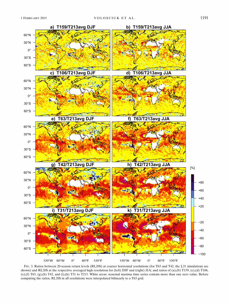
FIG. 3. Ratios between 20-season return levels (RL20S) at coarser horizontal resolutions (for T63 and T42, the L31 simulations are

shown) and RL20S at the respective averaged high resolution for (left) DJF and (right) JJA; and ratios of (a),(b) T159, (c),(d) T106,

(e),(f) T63, (g),(h) T42, and (i),(k) T31 to T213. White areas: seasonal maxima time series contain more than one zero value. Before

computing the ratios, RL20S in all resolutions were interpolated bilinearly to a T63 grid.

1 FEBRUARY 2015 VOLOSC IUK ET AL . 1191

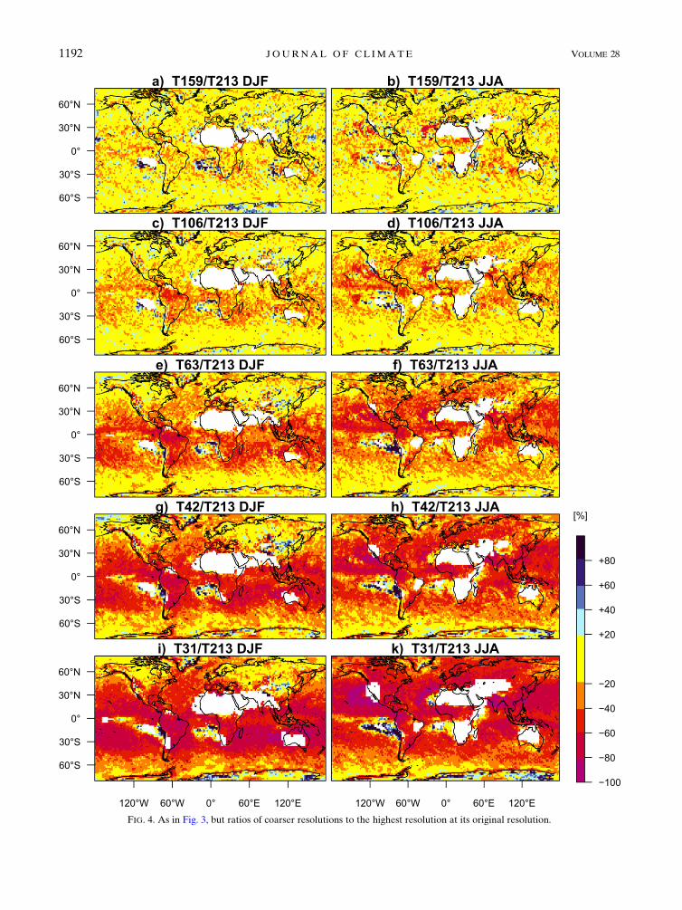
FIG. 4. As in Fig. 3, but ratios of coarser resolutions to the highest resolution at its original resolution.

1192 JOURNAL OF CL IMATE VOLUME 28

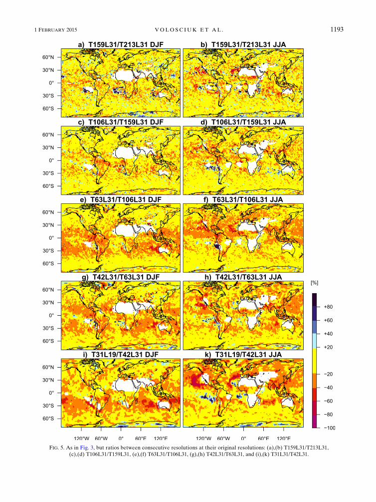
FIG. 5. As in Fig. 3, but ratios between consecutive resolutions at their original resolutions: (a),(b) T159L31/T213L31,

(c),(d) T106L31/T159L31, (e),(f) T63L31/T106L31, (g),(h) T42L31/T63L31, and (i),(k) T31L31/T42L31.

1 FEBRUARY 2015 VOLOSC IUK ET AL . 1193

c. Vertical resolution

Figure 2 shows that vertical resolution also has a re-

gionally varying impact on the representation of ex-

treme precipitation. Over northern Europe in DJF,

differences between the area averages of the RL20S at

different vertical resolutions are negligible, whereas in

the other regional examples the area average of the

RL20S at coarser vertical resolution is less than the area

average of the RL20S at higher vertical resolution. This

difference is more pronounced at T63 than at T42.

To further investigate the structure of changes in the

RL20S with vertical resolution, zonal means of the

RL20S (Fig. 6) of high vertical resolution (solid lines)

are compared with the RL20S of the low vertical reso-

lution (dashed lines). Coarser vertical resolution causes

a decrease in the RL20S. Additionally, the peak of ex-

treme tropical summer precipitation associated with the

ITCZ is shifted equatorward at coarser vertical resolu-

tion. This effect is stronger in boreal summer (JJA) than

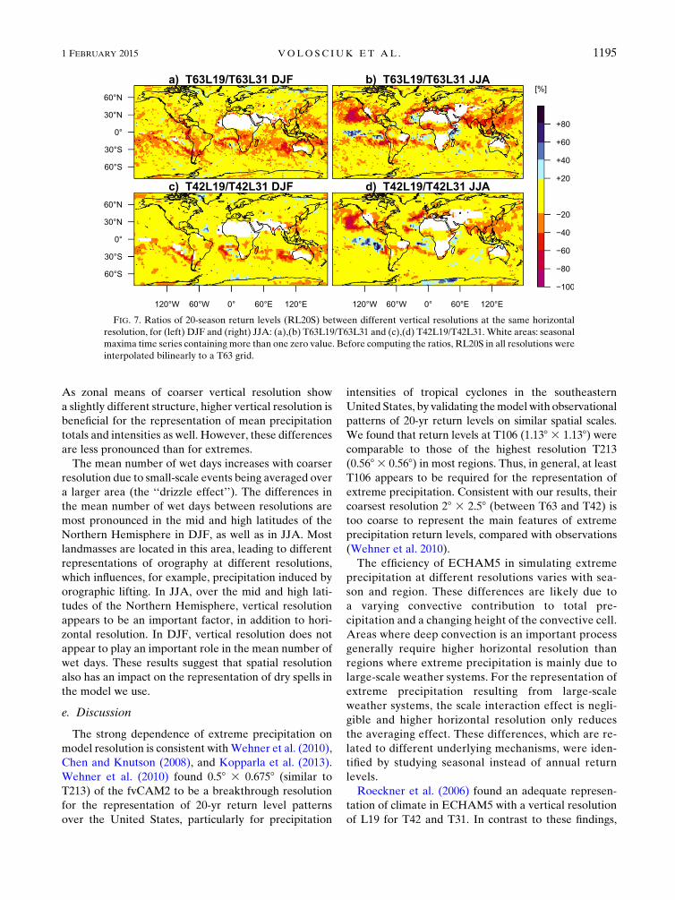
in austral summer (DJF). The spatial structure of

changes in extreme precipitation return levels with

vertical resolution is shown in Fig. 7. The impact of

vertical resolution is higher at T63 than at T42, consis-

tent with the regional examples (Fig. 2). High vertical

resolution is particularly important in a zonal band

around the ITCZ. For extreme precipitation associated

with the Asian monsoon, high vertical resolution is

crucial. However, over parts of the Northern Hemi-

sphere inDJF, coarser vertical resolution is sufficient for

the representation of the RL20S.

d. Comparison with mean precipitation

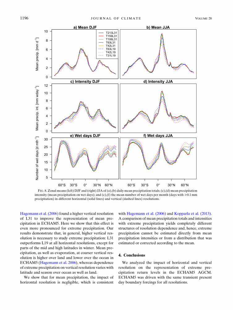
Figure 8 shows zonal means of mean precipitation

totals (Figs. 8a,b), mean precipitation intensities

(Figs. 8c,d) and themean number of wet days (Figs. 8e,f)

for DJF and JJA to study differences to the scale de-

pendence of extreme precipitation. The impact of hor-

izontal resolution onmean precipitation totals andmean

precipitation intensity is negligible. Peaks of the high

resolutions T213, T159, and T106 are similar; however,

coarser resolutions show slightly decreased peaks. Even

though these differences are small compared to those of

extremes, there is consistency regarding the large dif-

ferences between T106 and T63 observed for extremes.

FIG. 6. Zonal means of 20-season return levels (RL20S) for (left) DJF and (right) JJA: (a),(b) with different

horizontal (solid lines) and vertical (dashed lines) resolutions and (c),(d) additionally normalized with the zonal

mean of RL20S in the respective averaged high resolution. Grid boxes whose seasonal maxima time series contain

more than one zero value in at least one resolution are excluded in all resolutions.

1194 JOURNAL OF CL IMATE VOLUME 28

As zonal means of coarser vertical resolution show

a slightly different structure, higher vertical resolution is

beneficial for the representation of mean precipitation

totals and intensities as well. However, these differences

are less pronounced than for extremes.

The mean number of wet days increases with coarser

resolution due to small-scale events being averaged over

a larger area (the ‘‘drizzle effect’’). The differences in

the mean number of wet days between resolutions are

most pronounced in the mid and high latitudes of the

Northern Hemisphere in DJF, as well as in JJA. Most

landmasses are located in this area, leading to different

representations of orography at different resolutions,

which influences, for example, precipitation induced by

orographic lifting. In JJA, over the mid and high lati-

tudes of the Northern Hemisphere, vertical resolution

appears to be an important factor, in addition to hori-

zontal resolution. In DJF, vertical resolution does not

appear to play an important role in the mean number of

wet days. These results suggest that spatial resolution

also has an impact on the representation of dry spells in

the model we use.

e. Discussion

The strong dependence of extreme precipitation on

model resolution is consistent withWehner et al. (2010),

Chen and Knutson (2008), and Kopparla et al. (2013).

Wehner et al. (2010) found 0.58 3 0.6758 (similar to

T213) of the fvCAM2 to be a breakthrough resolution

for the representation of 20-yr return level patterns

over the United States, particularly for precipitation

intensities of tropical cyclones in the southeastern

United States, by validating themodelwith observational

patterns of 20-yr return levels on similar spatial scales.

We found that return levels at T106 (1.138 3 1.138) werecomparable to those of the highest resolution T213

(0.568 3 0.568) in most regions. Thus, in general, at least

T106 appears to be required for the representation of

extreme precipitation. Consistent with our results, their

coarsest resolution 28 3 2.58 (between T63 and T42) is

too coarse to represent the main features of extreme

precipitation return levels, compared with observations

(Wehner et al. 2010).

The efficiency of ECHAM5 in simulating extreme

precipitation at different resolutions varies with sea-

son and region. These differences are likely due to

a varying convective contribution to total pre-

cipitation and a changing height of the convective cell.

Areas where deep convection is an important process

generally require higher horizontal resolution than

regions where extreme precipitation is mainly due to

large-scale weather systems. For the representation of

extreme precipitation resulting from large-scale

weather systems, the scale interaction effect is negli-

gible and higher horizontal resolution only reduces

the averaging effect. These differences, which are re-

lated to different underlying mechanisms, were iden-

tified by studying seasonal instead of annual return

levels.

Roeckner et al. (2006) found an adequate represen-

tation of climate in ECHAM5 with a vertical resolution

of L19 for T42 and T31. In contrast to these findings,

FIG. 7. Ratios of 20-season return levels (RL20S) between different vertical resolutions at the same horizontal

resolution, for (left) DJF and (right) JJA: (a),(b) T63L19/T63L31 and (c),(d) T42L19/T42L31. White areas: seasonal

maxima time series containing more than one zero value. Before computing the ratios, RL20S in all resolutions were

interpolated bilinearly to a T63 grid.

1 FEBRUARY 2015 VOLOSC IUK ET AL . 1195

Hagemann et al. (2006) found a higher vertical resolution

of L31 to improve the representation of mean pre-

cipitation in ECHAM5. Here we show that this effect is

even more pronounced for extreme precipitation. Our

results demonstrate that, in general, higher vertical res-

olution is necessary to study extreme precipitation: L31

outperforms L19 at all horizontal resolutions, except for

parts of the mid and high latitudes in winter. Mean pre-

cipitation, as well as evaporation, at coarser vertical res-

olution is higher over land and lower over the ocean in

ECHAM5 (Hagemann et al. 2006), whereas dependence

of extreme precipitation on vertical resolution varies with

latitude and season over ocean as well as land.

We show that for mean precipitation, the impact of

horizontal resolution is negligible, which is consistent

with Hagemann et al. (2006) and Kopparla et al. (2013).

A comparison ofmean precipitation totals and intensities

with extreme precipitation yields completely different

structures of resolution dependence and, hence, extreme

precipitation cannot be estimated directly from mean

precipitation intensities or from a distribution that was

estimated or corrected according to the mean.

4. Conclusions

We analyzed the impact of horizontal and vertical

resolution on the representation of extreme pre-

cipitation return levels in the ECHAM5 AGCM.

ECHAM5 was driven with the same transient present

day boundary forcings for all resolutions.

FIG. 8. Zonal means (left) DJF and (right) JJA of (a),(b) daily mean precipitation totals; (c),(d) mean precipitation

intensity (mean precipitation on wet days); and (e),(f) the mean number of wet days per month (days with$0.1mm

precipitation) in different horizontal (solid lines) and vertical (dashed lines) resolutions.

1196 JOURNAL OF CL IMATE VOLUME 28

Decreasing horizontal resolution has several im-

pacts on extreme precipitation. First, increasing grid

size has the effect that precipitation is averaged over

a larger area (averaging effect). Second, in lower

horizontal resolutions the coarser representation of,

for instance, physical processes and orography yields

inferior representation of extreme precipitation (scale

interaction effect). Note that we do not intend to

identify the pure grid spacing effect, but rather define

the resolution effect as the overall effect of changing

grid spacing and tunable parameters. If one were in-

terested in a separation of the pure grid spacing, one

would have to carry out experiments as proposed by

Leung et al. (2013) and applied by, for example,

Rauscher et al. (2013). The highest resolution (T213)

averaged to coarser grid sizes (T213131–T213737: av-

eraged high resolution simulation, AHS) was com-

pared with coarser resolutions (T159–T31: coarser

resolution simulations, CRS). Differences between AHS

and CRS provide an approximate first-order discrimina-

tion between these two effects. Thereby, the relative im-

portance of both effects was determined. Twenty-season

return levels of daily precipitation (RL20S, derived

from a GEV distribution) in different resolutions were

compared.

Horizontal, as well as vertical, model resolution were

found to affect the representation of extreme pre-

cipitation. The averaging effect contributes consider-

ably to decreasing return levels with resolution. In the

belt of tropical summer extreme precipitation associated

with the ITCZ, averaging from T213 to T31 reduces the

RL20S by almost 30%. Hence, in accordance with Chen

and Knutson (2008), we strongly recommend comparing

extreme precipitation from different sources (e.g., dif-

ferent models, observations) only after averaging to the

same spatial scale. The scale interaction effect is stron-

gest in the summer hemisphere. In the band of extreme

precipitation associated with the ITCZ, the reduction

amounts to around 65% when changing the model res-

olution from T213 to T31. Toward middle to higher

latitudes, the scale interaction effect reduces to a de-

crease of about 20%. In the winter hemisphere it van-

ishes toward the poles.

The minimum required horizontal resolution for ex-

treme precipitation was found to depend on season and

region and, thus, mainly on the underlying process(es).

In general, extreme precipitation caused by small-scale

convective events requires higher horizontal resolution

than extreme precipitation caused by synoptic-scale

weather systems. Particularly in the tropics, but also in

the extratropics during summer, at least T106 is re-

quired to represent comparable return levels to the

highest resolution T213. Only marginal changes to

RL20S, caused by the averaging effect, were found in

the mid and high latitudes in winter, such as over parts

of the Northern Hemisphere’s landmass in DJF; here

RL20S in T31L19 are comparable to those in the

highest resolution (T213) on similar spatial scales.

Over wide areas of the mid and high latitudes during

winter (e.g., Canada and Asia in DJF), extreme pre-

cipitation was even found to be insensitive to changes

in resolution when comparing T31 with the highest

resolution (T213) at its original resolution.

Higher vertical resolution is crucial for the repre-

sentation of precipitation (consistent with Hagemann

et al. 2006). This applies particularly to the extremes,

as coarser vertical resolution causes an equatorward

shift of maximum extreme precipitation, as well as

a decrease in return levels. Therefore, we recommend

the use of higher vertical resolution for extreme

precipitation, even for relatively coarse horizontal

resolutions such as T42 or T63. Yet, the impact of

vertical resolution is more pronounced in T63 than

in T42. An exception is during winter in the mid

and high latitudes where RL20S in coarser vertical

resolution are comparable to those in high vertical

resolution.

Extreme precipitation shows a completely different

scale dependence to mean precipitation. The impact of

horizontal resolution on mean precipitation is negligi-

ble, whereas higher vertical resolution is still mean-

ingful but less pronounced than for the extremes. This

implies that extreme precipitation cannot be estimated

directly from mean precipitation intensities or from

a distribution that was estimated or corrected accord-

ing to the mean.

Here we present a model study where we take the

highest model resolution as reference for comparison

with the coarser model resolutions. This reference simu-

lation, in general, compares well with gridded observa-

tions, but also shows deficiencies in simulating the Asian

monsoon as well as orographic extreme precipitation,

which both tend to be overestimated. By construction, we

disregard effects not correctly simulated by the highest

considered resolution of the chosen model. In all con-

sidered resolutions, convection is parameterized. Thus,

related dynamical feedbacks are not resolved. Other

relevant processes for extremeprecipitation thatmight need

even higher resolution than all considered resolutions—

such as tropical cyclones (Wehner et al. 2010)—are be-

yond the scope of our study. Furthermore, climate

models may not fully capture important features of at-

mospheric dynamics related to extremes, in particular

persistent weather regimes (Petoukhov et al. 2013; Palmer

2013). Finally, as we have employed an atmosphere-only

model with prescribed ocean boundary conditions, ocean

1 FEBRUARY 2015 VOLOSC IUK ET AL . 1197

feedbacks are likewise not represented. Any recommen-

dations for minimum resolutions refer solely to the rep-

resentation of RL20S in an AGCM and do not imply that

the above listed phenomena are well represented at these

resolutions.

Although we have only studied the scaling be-

havior of extreme precipitation in one AGCM (i.e.,

ECHAM5), we believe that our results are also valid

for other AGCMs as physical explanations for the

scale dependence of extreme precipitation could be

identified.

Acknowledgments. The authors acknowledge help

with the simulations by W. Tseng, N. Keenlyside, and

G.Zhou.We thankM.Latif,A. Schindler, andE.Meredith

for helpful discussions as well as V. Lucarini and three

anonymous reviewers for comments on the manuscript.

Simulations were run at the North-German Super-

computing Alliance (HLRN). This study was funded by

the EUREX project of the Helmholtz Association

(HRJRG-308) and supported by Russian Foundation

for Basic Research (14-05-00518) and Russian Ministry

of Education and Science (Grant 14.B25.31.0026). The

GPCP combined precipitation data were developed and

computed by the NASA Goddard Space Flight Center

Laboratory for Atmospheres as a contribution to the

GEWEX Global Precipitation Climatology Project.

GPCP and CPC US Unified Precipitation data are

provided by the NOAA/OAR/ESRL PSD, Boulder,

Colorado, USA, from their Web site at http://www.esrl.

noaa.gov/psd/. We acknowledge the E-OBS dataset

from the EU-FP6 project ENSEMBLES (http://

ensembles-eu.metoffice.com) and the data providers in

the ECA&D project (http://eca.knmi.nl) as well as the

APHRODITE dataset and the data providers in the

APHRODITE’s Water Resources project (http://www.

chikyu.ac.jp/precip/).

APPENDIX

Uncertainties in the Return Levels

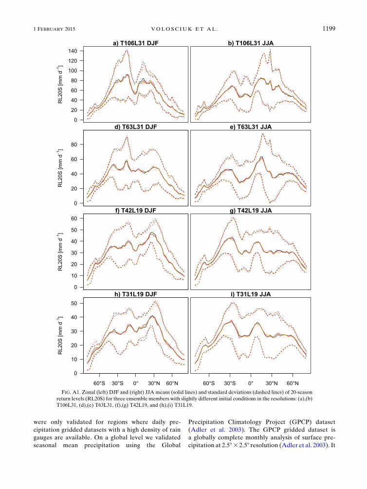
a. Internal model variability

One source of uncertainty in the estimation of

return levels is internal variability of the climate sys-

tem. To assess this unforced internal variability of the

climate model, long time series are required. As our

model runs are only 29 years long, due to limited

availability of the high-resolution boundary condi-

tions, we performed three ensemble members with

slightly different initial conditions for the resolutions

T106L31, T63L31, T42L19, and T31L19, which are

each 29 yr long. The difference between RL20S in

these three ensemble members yields uncertainties in

the return level estimation due to the climate model’s

internal variability. Figure A1 shows zonal means and

the respective zonal standard deviations of RL20S in

these three ensemble members for different resolutions.

Rather small differences between the zonal means of

the three ensemble members in all resolutions in DJF as

well as in JJA indicate that the forced climate is reliably

represented.

b. GEV sampling uncertainty

In this study, GEV parameters were estimated from

29 data points of 3-month-long blocks. This rather

small sample size may cause uncertainties in the return

levels. To assess these uncertainties, we applied

a parametric bootstrap method (Efron and Tibshirani

1993) to the highest (T213L31) and coarsest resolution

(T31L19) as follows. 1000 random time series (size: 29

data points, as in the actual sample), distributed ac-

cording to the fitted GEV distribution, were generated

for each grid box. Subsequently, GEV parameters for

each time series were estimated. The 95% confidence

interval of the empirical distribution of RL20S in these

1000 realizations quantifies the GEV parameter un-

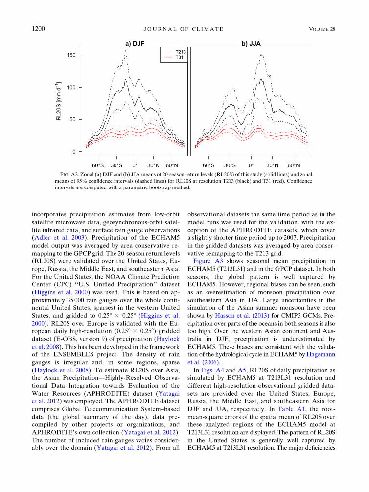
certainties of RL20S. Figure A2 shows the zonal mean

of RL20S in this study (solid lines) and the zonal mean

of the gridbox-wise 95% confidence intervals derived

from the bootstrap method (dashed lines); that is, the

latitude-dependent mean parameter uncertainty of

a grid box is shown. The confidence intervals are quite

symmetric and indicate an acceptable spread, which

gives us confidence in our return level estimates. Note

that this is the parameter uncertainty of the mean grid

box at a given latitude. Under the assumption that the

empirical distribution is symmetric and the samples

are independent, the parameter uncertainty of the

zonal mean is related to the zonal mean of the pa-

rameter uncertainty by a scaling factor of 1/ffiffiffin

p(ac-

cording to Gaussian error propagation). Thus,

sampling uncertainties for the zonal mean (see

Fig. A2) are negligible.

c. Validation of the highest resolution of ECHAM5with observational datasets

To assess the performance of the highest resolution

(T213L31) of ECHAM5, which is used as reference for

the coarser resolutions in our study, we validated

model precipitation with gridded observational data-

sets. As no global daily precipitation dataset with

sufficient density of rain gauges is available to reliably

estimate extreme precipitation return levels, the latter

1198 JOURNAL OF CL IMATE VOLUME 28

were only validated for regions where daily pre-

cipitation gridded datasets with a high density of rain

gauges are available. On a global level we validated

seasonal mean precipitation using the Global

Precipitation Climatology Project (GPCP) dataset

(Adler et al. 2003). The GPCP gridded dataset is

a globally complete monthly analysis of surface pre-

cipitation at 2.58 3 2.58 resolution (Adler et al. 2003). It

FIG. A1. Zonal (left) DJF and (right) JJA means (solid lines) and standard deviations (dashed lines) of 20-season

return levels (RL20S) for three ensemble members with slightly different initial conditions in the resolutions: (a),(b)

T106L31, (d),(e) T63L31, (f),(g) T42L19, and (h),(i) T31L19.

1 FEBRUARY 2015 VOLOSC IUK ET AL . 1199

incorporates precipitation estimates from low-orbit

satellite microwave data, geosynchronous-orbit satel-

lite infrared data, and surface rain gauge observations

(Adler et al. 2003). Precipitation of the ECHAM5

model output was averaged by area conservative re-

mapping to theGPCP grid. The 20-season return levels

(RL20S) were validated over the United States, Eu-

rope, Russia, the Middle East, and southeastern Asia.

For the United States, the NOAA Climate Prediction

Center (CPC) ‘‘U.S. Unified Precipitation’’ dataset

(Higgins et al. 2000) was used. This is based on ap-

proximately 35 000 rain gauges over the whole conti-

nental United States, sparsest in the western United

States, and gridded to 0.258 3 0.258 (Higgins et al.

2000). RL20S over Europe is validated with the Eu-

ropean daily high-resolution (0.258 3 0.258) gridded

dataset (E-OBS, version 9) of precipitation (Haylock

et al. 2008). This has been developed in the framework

of the ENSEMBLES project. The density of rain

gauges is irregular and, in some regions, sparse

(Haylock et al. 2008). To estimate RL20S over Asia,

the Asian Precipitation—Highly-Resolved Observa-

tional Data Integration towards Evaluation of the

Water Resources (APHRODITE) dataset (Yatagai

et al. 2012) was employed. The APHRODITE dataset

comprises Global Telecommunication System–based

data (the global summary of the day), data pre-

compiled by other projects or organizations, and

APHRODITE’s own collection (Yatagai et al. 2012).

The number of included rain gauges varies consider-

ably over the domain (Yatagai et al. 2012). From all

observational datasets the same time period as in the

model runs was used for the validation, with the ex-

ception of the APHRODITE datasets, which cover

a slightly shorter time period up to 2007. Precipitation

in the gridded datasets was averaged by area conser-

vative remapping to the T213 grid.

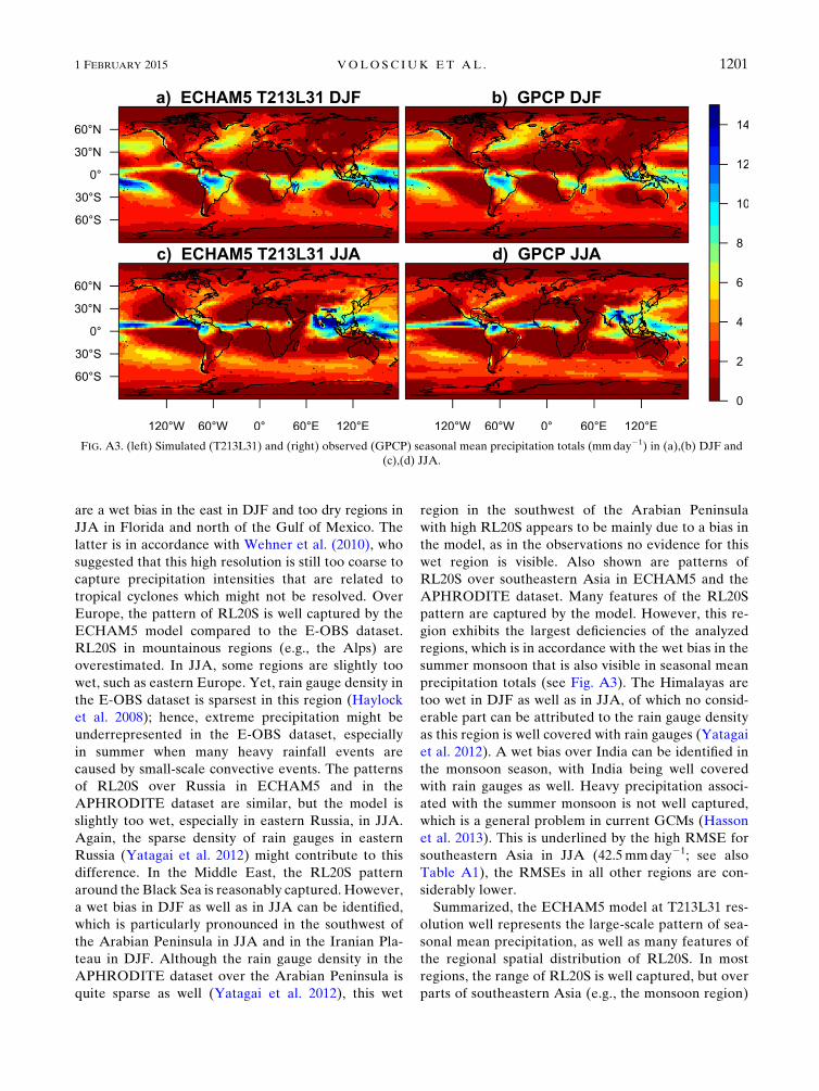
Figure A3 shows seasonal mean precipitation in

ECHAM5 (T213L31) and in the GPCP dataset. In both

seasons, the global pattern is well captured by

ECHAM5. However, regional biases can be seen, such

as an overestimation of monsoon precipitation over

southeastern Asia in JJA. Large uncertainties in the

simulation of the Asian summer monsoon have been

shown by Hasson et al. (2013) for CMIP3 GCMs. Pre-

cipitation over parts of the oceans in both seasons is also

too high. Over the western Asian continent and Aus-

tralia in DJF, precipitation is underestimated by

ECHAM5. These biases are consistent with the valida-

tion of the hydrological cycle in ECHAM5 byHagemann

et al. (2006).

In Figs. A4 and A5, RL20S of daily precipitation as

simulated by ECHAM5 at T213L31 resolution and

different high-resolution observational gridded data-

sets are provided over the United States, Europe,

Russia, the Middle East, and southeastern Asia for

DJF and JJA, respectively. In Table A1, the root-

mean-square errors of the spatial mean of RL20S over

these analyzed regions of the ECHAM5 model at

T213L31 resolution are displayed. The pattern of RL20S

in the United States is generally well captured by

ECHAM5 at T213L31 resolution. The major deficiencies

FIG. A2. Zonal (a) DJF and (b) JJA means of 20-season return levels (RL20S) of this study (solid lines) and zonal

means of 95% confidence intervals (dashed lines) for RL20S at resolution T213 (black) and T31 (red). Confidence

intervals are computed with a parametric bootstrap method.

1200 JOURNAL OF CL IMATE VOLUME 28

are a wet bias in the east in DJF and too dry regions in

JJA in Florida and north of the Gulf of Mexico. The

latter is in accordance with Wehner et al. (2010), who

suggested that this high resolution is still too coarse to

capture precipitation intensities that are related to

tropical cyclones which might not be resolved. Over

Europe, the pattern of RL20S is well captured by the

ECHAM5 model compared to the E-OBS dataset.

RL20S in mountainous regions (e.g., the Alps) are

overestimated. In JJA, some regions are slightly too

wet, such as eastern Europe. Yet, rain gauge density in

the E-OBS dataset is sparsest in this region (Haylock

et al. 2008); hence, extreme precipitation might be

underrepresented in the E-OBS dataset, especially

in summer when many heavy rainfall events are

caused by small-scale convective events. The patterns

of RL20S over Russia in ECHAM5 and in the

APHRODITE dataset are similar, but the model is

slightly too wet, especially in eastern Russia, in JJA.

Again, the sparse density of rain gauges in eastern

Russia (Yatagai et al. 2012) might contribute to this

difference. In the Middle East, the RL20S pattern

around the Black Sea is reasonably captured. However,

a wet bias in DJF as well as in JJA can be identified,

which is particularly pronounced in the southwest of

the Arabian Peninsula in JJA and in the Iranian Pla-

teau in DJF. Although the rain gauge density in the

APHRODITE dataset over the Arabian Peninsula is

quite sparse as well (Yatagai et al. 2012), this wet

region in the southwest of the Arabian Peninsula

with high RL20S appears to be mainly due to a bias in

the model, as in the observations no evidence for this

wet region is visible. Also shown are patterns of

RL20S over southeastern Asia in ECHAM5 and the

APHRODITE dataset. Many features of the RL20S

pattern are captured by the model. However, this re-

gion exhibits the largest deficiencies of the analyzed

regions, which is in accordance with the wet bias in the

summer monsoon that is also visible in seasonal mean

precipitation totals (see Fig. A3). The Himalayas are

too wet in DJF as well as in JJA, of which no consid-

erable part can be attributed to the rain gauge density

as this region is well covered with rain gauges (Yatagai

et al. 2012). A wet bias over India can be identified in

the monsoon season, with India being well covered

with rain gauges as well. Heavy precipitation associ-

ated with the summer monsoon is not well captured,

which is a general problem in current GCMs (Hasson

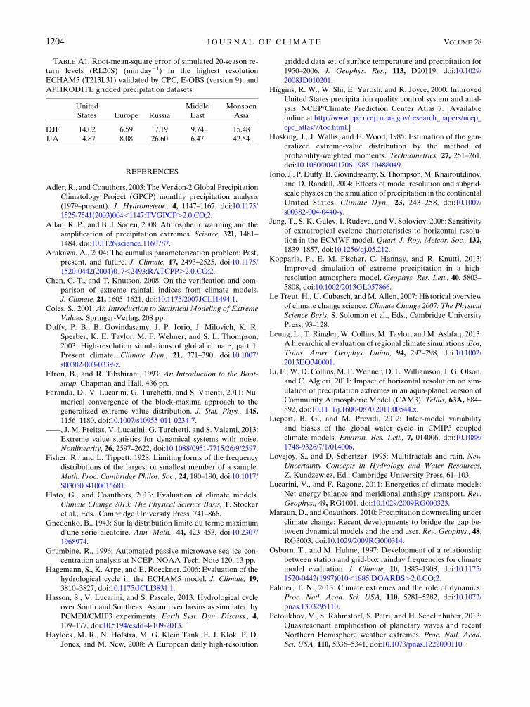
et al. 2013). This is underlined by the high RMSE for

southeastern Asia in JJA (42.5mmday21; see also

Table A1), the RMSEs in all other regions are con-

siderably lower.

Summarized, the ECHAM5 model at T213L31 res-

olution well represents the large-scale pattern of sea-

sonal mean precipitation, as well as many features of

the regional spatial distribution of RL20S. In most

regions, the range of RL20S is well captured, but over

parts of southeastern Asia (e.g., the monsoon region)

FIG. A3. (left) Simulated (T213L31) and (right) observed (GPCP) seasonal mean precipitation totals (mmday21) in (a),(b) DJF and

(c),(d) JJA.

1 FEBRUARY 2015 VOLOSC IUK ET AL . 1201

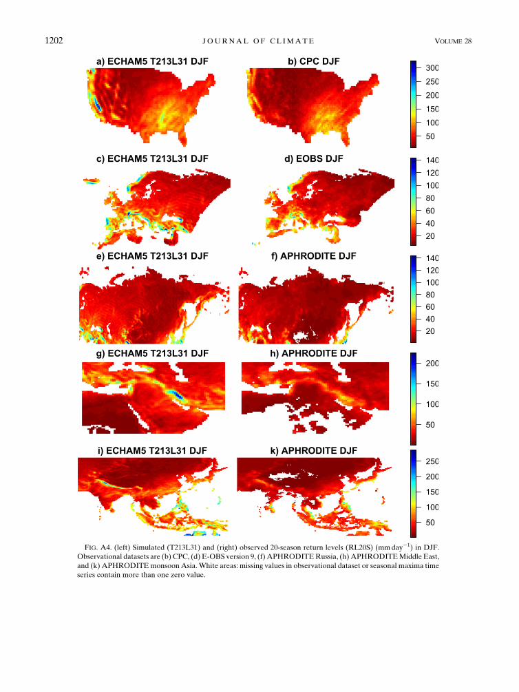
FIG. A4. (left) Simulated (T213L31) and (right) observed 20-season return levels (RL20S) (mmday21) in DJF.

Observational datasets are (b) CPC, (d) E-OBS version 9, (f) APHRODITERussia, (h)APHRODITEMiddle East,

and (k) APHRODITEmonsoonAsia. White areas: missing values in observational dataset or seasonal maxima time

series contain more than one zero value.

1202 JOURNAL OF CL IMATE VOLUME 28

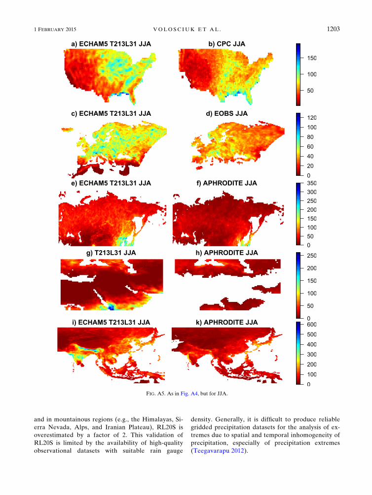
and in mountainous regions (e.g., the Himalayas, Si-

erra Nevada, Alps, and Iranian Plateau), RL20S is

overestimated by a factor of 2. This validation of

RL20S is limited by the availability of high-quality

observational datasets with suitable rain gauge

density. Generally, it is difficult to produce reliable

gridded precipitation datasets for the analysis of ex-

tremes due to spatial and temporal inhomogeneity of

precipitation, especially of precipitation extremes

(Teegavarapu 2012).

FIG. A5. As in Fig. A4, but for JJA.

1 FEBRUARY 2015 VOLOSC IUK ET AL . 1203

REFERENCES

Adler, R., and Coauthors, 2003: The Version-2 Global Precipitation

Climatology Project (GPCP) monthly precipitation analysis

(1979–present). J. Hydrometeor., 4, 1147–1167, doi:10.1175/

1525-7541(2003)004,1147:TVGPCP.2.0.CO;2.

Allan, R. P., and B. J. Soden, 2008: Atmospheric warming and the

amplification of precipitation extremes. Science, 321, 1481–

1484, doi:10.1126/science.1160787.

Arakawa, A., 2004: The cumulus parameterization problem: Past,

present, and future. J. Climate, 17, 2493–2525, doi:10.1175/

1520-0442(2004)017,2493:RATCPP.2.0.CO;2.

Chen, C.-T., and T. Knutson, 2008: On the verification and com-

parison of extreme rainfall indices from climate models.

J. Climate, 21, 1605–1621, doi:10.1175/2007JCLI1494.1.

Coles, S., 2001: An Introduction to Statistical Modeling of Extreme

Values. Springer-Verlag, 208 pp.

Duffy, P. B., B. Govindasamy, J. P. Iorio, J. Milovich, K. R.

Sperber, K. E. Taylor, M. F. Wehner, and S. L. Thompson,

2003: High-resolution simulations of global climate, part 1:

Present climate. Climate Dyn., 21, 371–390, doi:10.1007/

s00382-003-0339-z.

Efron, B., and R. Tibshirani, 1993: An Introduction to the Boot-

strap. Chapman and Hall, 436 pp.

Faranda, D., V. Lucarini, G. Turchetti, and S. Vaienti, 2011: Nu-

merical convergence of the block-maxima approach to the

generalized extreme value distribution. J. Stat. Phys., 145,1156–1180, doi:10.1007/s10955-011-0234-7.

——, J. M. Freitas, V. Lucarini, G. Turchetti, and S. Vaienti, 2013:

Extreme value statistics for dynamical systems with noise.

Nonlinearity, 26, 2597–2622, doi:10.1088/0951-7715/26/9/2597.Fisher, R., and L. Tippett, 1928: Limiting forms of the frequency

distributions of the largest or smallest member of a sample.

Math. Proc. Cambridge Philos. Soc., 24, 180–190, doi:10.1017/

S0305004100015681.

Flato, G., and Coauthors, 2013: Evaluation of climate models.

Climate Change 2013: The Physical Science Basis, T. Stocker

et al., Eds., Cambridge University Press, 741–866.

Gnedenko, B., 1943: Sur la distribution limite du terme maximum

d’une série aléatoire. Ann. Math., 44, 423–453, doi:10.2307/

1968974.

Grumbine, R., 1996: Automated passive microwave sea ice con-

centration analysis at NCEP. NOAA Tech. Note 120, 13 pp.

Hagemann, S., K. Arpe, and E. Roeckner, 2006: Evaluation of the

hydrological cycle in the ECHAM5 model. J. Climate, 19,

3810–3827, doi:10.1175/JCLI3831.1.

Hasson, S., V. Lucarini, and S. Pascale, 2013: Hydrological cycle

over South and Southeast Asian river basins as simulated by

PCMDI/CMIP3 experiments. Earth Syst. Dyn. Discuss., 4,109–177, doi:10.5194/esdd-4-109-2013.

Haylock, M. R., N. Hofstra, M. G. Klein Tank, E. J. Klok, P. D.

Jones, and M. New, 2008: A European daily high-resolution

gridded data set of surface temperature and precipitation for

1950–2006. J. Geophys. Res., 113, D20119, doi:10.1029/

2008JD010201.

Higgins, R. W., W. Shi, E. Yarosh, and R. Joyce, 2000: Improved

United States precipitation quality control system and anal-

ysis. NCEP/Climate Prediction Center Atlas 7. [Available

online at http://www.cpc.ncep.noaa.gov/research_papers/ncep_

cpc_atlas/7/toc.html.]

Hosking, J., J. Wallis, and E. Wood, 1985: Estimation of the gen-

eralized extreme-value distribution by the method of

probability-weighted moments. Technometrics, 27, 251–261,

doi:10.1080/00401706.1985.10488049.

Iorio, J., P. Duffy, B. Govindasamy, S. Thompson,M. Khairoutdinov,

and D. Randall, 2004: Effects of model resolution and subgrid-

scale physics on the simulation of precipitation in the continental

United States. Climate Dyn., 23, 243–258, doi:10.1007/

s00382-004-0440-y.

Jung, T., S. K. Gulev, I. Rudeva, and V. Soloviov, 2006: Sensitivity

of extratropical cyclone characteristics to horizontal resolu-

tion in the ECMWF model. Quart. J. Roy. Meteor. Soc., 132,

1839–1857, doi:10.1256/qj.05.212.

Kopparla, P., E. M. Fischer, C. Hannay, and R. Knutti, 2013:

Improved simulation of extreme precipitation in a high-

resolution atmosphere model. Geophys. Res. Lett., 40, 5803–

5808, doi:10.1002/2013GL057866.

Le Treut, H., U. Cubasch, and M. Allen, 2007: Historical overview

of climate change science. Climate Change 2007: The Physical

Science Basis, S. Solomon et al., Eds., Cambridge University

Press, 93–128.

Leung, L., T. Ringler, W. Collins, M. Taylor, and M. Ashfaq, 2013:

A hierarchical evaluation of regional climate simulations.Eos,

Trans. Amer. Geophys. Union, 94, 297–298, doi:10.1002/

2013EO340001.

Li, F., W. D. Collins, M. F. Wehner, D. L. Williamson, J. G. Olson,

and C. Algieri, 2011: Impact of horizontal resolution on sim-

ulation of precipitation extremes in an aqua-planet version of

Community Atmospheric Model (CAM3). Tellus, 63A, 884–

892, doi:10.1111/j.1600-0870.2011.00544.x.

Liepert, B. G., and M. Previdi, 2012: Inter-model variability

and biases of the global water cycle in CMIP3 coupled

climate models. Environ. Res. Lett., 7, 014006, doi:10.1088/

1748-9326/7/1/014006.

Lovejoy, S., and D. Schertzer, 1995: Multifractals and rain. New

Uncertainty Concepts in Hydrology and Water Resources,

Z. Kundzewicz, Ed., Cambridge University Press, 61–103.

Lucarini, V., and F. Ragone, 2011: Energetics of climate models:

Net energy balance and meridional enthalpy transport. Rev.

Geophys., 49, RG1001, doi:10.1029/2009RG000323.

Maraun, D., and Coauthors, 2010: Precipitation downscaling under

climate change: Recent developments to bridge the gap be-

tween dynamical models and the end user. Rev. Geophys., 48,

RG3003, doi:10.1029/2009RG000314.

Osborn, T., and M. Hulme, 1997: Development of a relationship

between station and grid-box rainday frequencies for climate

model evaluation. J. Climate, 10, 1885–1908, doi:10.1175/

1520-0442(1997)010,1885:DOARBS.2.0.CO;2.

Palmer, T. N., 2013: Climate extremes and the role of dynamics.

Proc. Natl. Acad. Sci. USA, 110, 5281–5282, doi:10.1073/

pnas.1303295110.

Petoukhov, V., S. Rahmstorf, S. Petri, and H. Schellnhuber, 2013:

Quasiresonant amplification of planetary waves and recent

Northern Hemisphere weather extremes. Proc. Natl. Acad.

Sci. USA, 110, 5336–5341, doi:10.1073/pnas.1222000110.

TABLE A1. Root-mean-square error of simulated 20-season re-

turn levels (RL20S) (mmday21) in the highest resolution

ECHAM5 (T213L31) validated by CPC, E-OBS (version 9), and

APHRODITE gridded precipitation datasets.

United

States Europe Russia

Middle

East

Monsoon

Asia

DJF 14.02 6.59 7.19 9.74 15.48

JJA 4.87 8.08 26.60 6.47 42.54

1204 JOURNAL OF CL IMATE VOLUME 28

Pope, V., and R. Stratton, 2002: The processes governing hori-

zontal resolution sensitivity in a climate model. Climate Dyn.,

19, 211–236, doi:10.1007/s00382-001-0222-8.

Prein, A. F., G. J. Holland, R. M. Rasmussen, J. Done, K. Ikeda,

M. P. Clark, and C. H. Liu, 2013: Importance of regional

climate model grid spacing for the simulation of heavy pre-

cipitation in the Colorado headwaters. J. Climate, 26, 4848–

4857, doi:10.1175/JCLI-D-12-00727.1.

Randall, D., and Coauthors, 2007: Climate models and their eval-

uation. Climate Change 2007: The Physical Science Basis,

S. Solomon et al., Eds., Cambridge University Press, 589–662.

Rauscher, S., T. Ringler, W. Skamarock, and A. Mirin, 2013: Ex-

ploring a global multiresolution modeling approach using

aquaplanet simulations. J. Climate, 26, 2432–2452, doi:10.1175/

JCLI-D-12-00154.1.

R Development Core Team, 2011: R: A Language and Environ-

ment for Statistical Computing. R Foundation for Statistical

Computing. [Available online at http://www.r-project.org/.]

Reynolds, R. W., T. M. Smith, C. Liu, D. B. Chelton, K. S. Casey,

and M. G. Schlax, 2007: Daily high-resolution-blended anal-

yses for sea surface temperature. J. Climate, 20, 5473–5496,

doi:10.1175/2007JCLI1824.1.

Roeckner, E., and Coauthors, 2003: The atmospheric general cir-

culation model ECHAM5. Part I: Model description. MPI

Rep. 349, Max-Planck-Institute for Meteorology, 127 pp.

——, and Coauthors, 2004: The atmospheric general circulation

model ECHAM5. Part II: Sensitivity of simulated climate to

horizontal and vertical resolution.MPIRep. 354,Max-Planck-

Institute for Meteorology, 55 pp.

——, and Coauthors, 2006: Sensitivity of simulated climate to hori-

zontal and vertical resolution in the ECHAM5 atmosphere

model. J. Climate, 19, 3771–3791, doi:10.1175/JCLI3824.1.

Rummukainen, M., 2010: State-of-the-art with regional climate models.

Wiley Interdiscip.Rev.:ClimateChange, 1,82–96, doi:10.1002/wcc.8.

Rust, H. W., 2009: The effect of long-range dependence on mod-

elling extremes with the generalised extreme value distribu-

tion. Eur. Phys. J. Spec. Top., 174, 91–97, doi:10.1140/

epjst/e2009-01092-8.

Seneviratne, S. I., and Coauthors, 2012: Changes in climate ex-

tremes and their impacts on the natural physical environment.

Managing the Risks of Extreme Events and Disasters to Ad-

vance Climate Change Adaptation, C. Field et al., Eds., Cam-

bridge University Press, 109–230.

Smith, I., A. Moise, J. Katzfey, K. Nguyen, and R. Colman, 2013:

Regional-scale rainfall projections: Simulations for the New

Guinea region using the CCAM model. J. Geophys. Res. At-

mos., 118, 1271–1280, doi:10.1002/jgrd.50139.

Sun, Y., S. Solomon, A. Dai, and R. Portmann, 2006: How

often does it rain? J. Climate, 19, 916–934, doi:10.1175/

JCLI3672.1.

Teegavarapu, R. S., 2012: Floods in a Changing Climate. Cam-

bridge University Press, 269 pp.

Wehner, M. F., R. L. Smith, G. Bala, and P. Duffy, 2010: The effect

of horizontal resolution on simulation of very extreme US

precipitation events in a global atmosphere model. Climate

Dyn., 34, 241–247, doi:10.1007/s00382-009-0656-y.

Williamson, D. L., 2008: Convergence of aqua-planet simula-

tions with increasing resolution in the Community Atmo-

spheric Model, version 3. Tellus, 60A, 848–862, doi:10.1111/

j.1600-0870.2008.00339.x.

Wuertz, D., and Coauthors, 2009: fExtremes: Rmetrics—Extreme

financial market data. [Available online at http://

cran.r-project.org/web/packages/fExtremes/index.html.]

Yatagai, A., K. Kamiguchi, O.Arakawa, A.Hamada, N. Yasutomi,

and A. Kitoh, 2012: APHRODITE: Constructing a long-term

daily gridded precipitation dataset for Asia based on a dense

network of rain gauges. Bull. Amer. Meteor. Soc., 93, 1401–

1415, doi:10.1175/BAMS-D-11-00122.1.

1 FEBRUARY 2015 VOLOSC IUK ET AL . 1205