extracting information from sequences of spatially...

Ultramicroscopy 77 (1999) 97}112

Extracting information from sequences of spatially resolvedEELS spectra using multivariate statistical analysis

N. Bonnet!, N. Brun",*, C. Colliex",#

!Unite& INSERM 314 (IFR 53) and LERI, 21 rue Cle&ment Ader, 51685 Reims Cedex 2, France"Laboratoire de Physique des Solides, CNRS URA 002, BaL timent 510, Universite& Paris Sud, 91405 Orsay Cedex, France

#Laboratoire Aime& Cotton, CNRS UPR 3321, BaL timent 505, Universite& Paris Sud, 91405 Orsay Cedex, France

Received 27 May 1998; received in revised form 22 February 1999

Abstract

The sophisticated acquisition procedures now available in spatially or time resolved spectroscopies produce largeamounts of data which require e$cient automatic data processing procedures. In an electron energy loss spectroscopy(EELS) line-spectrum sequence, all individual spectra can be processed independently. However, it is better to considerthe data set as a whole and to process it as such. Multivariate statistical analysis (MSA) can be used to identify severalbasic sources of information as contributing through a linear combination to the overall experimental data set. In thispaper we show that MSA can be applied to spatially resolved spectroscopy, but often necessitates that extension fromorthogonal to oblique analysis be performed. The aim is then to identify "ne structures characteristic of EELS edges andto extract the signal speci"c of the interface. In the "rst section we present the overall methodology. Then it is illustratedthrough a simulation. Finally, we apply the method to the study of Si}SiO

2and SiO

2}TiO

2interfaces. We show that

MSA constitutes a useful tool to estimate components present at the interface and the corresponding concentrationpro"le of these components. ( 1999 Elsevier Science B.V. All rights reserved.

PACS: 61.16.Bg; 68.35.Dv; 82.80.Pv; 02.50.Sk

Keywords: EELS; Multivariate statistical analysis; Interface

1. Introduction

Electron energy loss spectroscopy (EELS) allowsto study local chemical and electronic properties ofa specimen with a very high resolution. Beyondelemental mapping, the greatest potential use of thespatially resolved EELS lies in its ability of display-

*Corresponding author. Tel.: #33-1-69155368; fax: #33-1-69158004.

E-mail address: [email protected] (N. Brun)

ing the distribution of the di!erent "ne structures,in order to determine the changes in structure,chemistry and bonding states in the near interfaceregion. In the line-spectrum mode, the probe isscanned across the interface and a spectrum re-corded for each position of the probe. When inves-tigating the detailed chemistry and electron statesfeatures across an interface, the most importantinformation lies in the variation between successivespectra corresponding to di!erent positions of theprobe. This data acquisition procedure has provedto be very e$cient during the past few years [1}3].

0304-3991/99/$ - see front matter ( 1999 Elsevier Science B.V. All rights reserved.PII: S 0 3 0 4 - 3 9 9 1 ( 9 9 ) 0 0 0 4 2 - X

In order to realize the best sampling for an in-homogeneous specimen, one takes care to workwith conditions close to the optimum samplingones, i.e. with the step between two measurementsof the order of the radius of the probe.

These sophisticated acquisition schemes nowavailable in microanalysis produce large amountsof data which also necessitate e$cient automatic(or semi-automatic) data processing procedures.Series of spectra recorded across an interface, withthe line-spectrum technique, are examples of suchdata sets. Several methods have been previouslysuggested for analyzing the content of these linespectra. The di!erent spectra of the set can beprocessed independently, along the ways of classi-cal spectroscopy (modelling and subtracting thebackground; "tting the spectrum to a sum of back-ground and characteristic signal models;2) [2,4].Pairs of spectra can also be considered and ana-lyzed according to the di!erence method [5}7].A neural pattern recognition technique was alsosuggested [8]. Although the spectra of a line-spec-trum series can be analyzed independently, it isbetter to consider the data set as a whole and toprocess it as such. For this purpose several ap-proaches are available, pertaining to multivariateanalysis, pattern recognition, clustering and/orneural computation. Although we have exploredthese di!erent alternatives, we put emphasis in thisreport on multivariate statistical analysis (MSA).The aim of MSA is to identify several basic sourcesof information as contributing (through a linearcombination) to the overall experimental data set.The validity of this basic assumption can be ques-tioned when the spectral answer of the specimen isnon-local, in which case the linear combinationdescription may be broken. For instance, we havedemonstrated in a recent paper [9] that the weightof an interface collective mode between two media(Si/SiO

2) requires a more extensive description as

a function of the impact parameter. The MSAapproach has already been sucessfully applied toenergy-"ltered image series [10,11], to spectrumlines and images [12,13] and to chrono-spectro-scopy [14]. It has also applied to sets of spatiallyrecorded X-ray spectra [15,16].

Our aim is to study "ne structures characteristicof EELS edges and to extract the signal speci"c to

Fig. 1. 3D representation of the spectrum-line made of 64spectra collected across the Si/SiO

2interface.

Fig. 2. 3D representation of the spectrum-line made of 64spectra collected across the TiO

2/SiO

2interface.

the interface. In the case of a chemically perfectinterface, i.e. when no other phase is present at theinterface, the signals arising from di!erent atomsare supposed to add up linearly, so it is possibleto describe each spectrum of the series as a linearcombination of two models. If a new phase is for-med at the interface, with atoms having a speci"c

98 N. Bonnet et al. / Ultramicroscopy 77 (1999) 97}112

environment, a "ne structures characteristic of theinterface should be recorded.

In this paper, we show that MSA can be appliedto spatially resolved spectroscopy, but often neces-sitates that the extension from orthogonal tooblique analysis is performed. In the next section,we present the overall methodology and we illus-trate it through a simulation. Finally, we apply themethod to the study of three interfaces: one of themconcerns an Si}SiO

2interface (Fig. 1) and the other

two concern SiO2}TiO

2interfaces (Fig. 2).

2. Description of the simulated data set

In order to illustrate the methodology describedin the next section, we have simulated a series of 21spectra as a linear combination of three compo-nents. Two of these components (supposed to cor-respond to the end-points of the series) are Si andSiO

2electron energy loss spectra over the

99}124 eV range, corresponding to the Si L2,3

edge.The third (hypothetical) component is composed oftwo Gaussian bumps (see Fig. 3). The resultingspectrum series is displayed in Fig. 4. The weightsof the three components are shown in Fig. 5.

3. Methodology for analyzing line spectra by MSA

The application of MSA to spatially resolvedspectroscopy can be done along the following lines:

Fig. 3. Simulated spectrum of an hypothetical (unknown) com-ponent situated in the core part of an interface.

Fig. 4. Spectrum series simulated from the linear combinationof real spectra Si and SiO

2and of the simulated spectrum

displayed in Fig. 3 (the coe$cients of the combination aredisplayed in Fig. 5). The aim of the analysis is to deduce theunknown spectrum at the interface and the composition vari-ations across the interface.

Fig. 5. Plot of the simulated concentration variations (for thethree components) across the interface.

f First, an orthogonal analysis is performed:through an eigenvector decomposition of thevariance}covariance matrix, a new representa-tion space is de"ned. This is done in such a waythat the "rst axis of representation correspondsto the direction (in the parameter space) with thehighest intensity variance, the second axis cor-responds to the direction with the highest resid-ual variance, etc. Each of these new directions ofspace will be referred to as a source of informa-tion. (In fact, due to the redundancy present in

N. Bonnet et al. / Ultramicroscopy 77 (1999) 97}112 99

the data set, only a limited number of axes carrya large amount of information. The other axesare mainly representative of noise.)

f When only one source of information is present,the interpretation of the data set is easy anddirectly quantitative (the scores of the di!erentspectra on the main factorial axes provide thewanted coe$cients, which help in quantifyingthe concentrations). But when several sources ofinformation are present, the orthogonal de-composition must often be followed by a nextstep (called factor analysis (FA) or oblique analy-sis), because the real sources of information arenot necessarily orthogonal [17].

3.1. Orthogonal analysis

MSA is a statistical method which aims toanalyze the variances and covariances of a multi-dimensional data set, a set of several related spectraor images for instance. Since such data sets oftencontain a large amount of redundancy, the aim isalso to de"ne their `truea dimensionality (i.e. thenumber of independent components, or sources ofinformation). This can be done along the followinglines:

f We represent the data set by a matrix X"MXnjN.

The lines n of this matrix are the spectra(n"1,2, N) and the columns j are the energychannels ( j"1,2, P).

f First, the variance}covariance matrix > of thedata set is built:

>"X )Xt. (1)

The variance}covariance matrix > is a (square)matrix (N]N), whose number of lines (and col-umns) is the number of spectra, and which con-tains the variance of the di!erent spectra (alongthe diagonal) and the covariances correspondingto pairs of spectra, i.e. the amount of informationshared by pairs of spectra.

f Second, the eigenvalue decomposition of thismatrix is performed. The eigenvectorsSnk

(n"1,2, N; k"0,2, N!1) constitute anew representation space for the data. Thenumber of signi"cant eigenvalues (K(N)

corresponds to the dimensionality (number ofsources of information, or degrees of freedom) ofthe data set.

Several tools are available for performing theinterpretation of the eigenvector decomposition.First, the coordinates t

nkof the di!erent spectra on

the new representation space can be used: this helpsto understand how the di!erent spectra are relatedto each other. In the case of spatially resolvedspectroscopy, this is related to a spatial analysis(which spatial information is carried by the di!er-ent sources?). Second, the coordinates of the energychannels on the new representation space can becomputed as

U"Xt )S or /kj"+

n

Xnj) S

nk

(n"1,2,N) ( j"1,2,P) (k"0,2,K!1). (2)

(The formulae reported in this section refer to prin-cipal components analysis. In this case, >

nk"S

nk.

Similar, but di!erent, expressions hold for othervariants of MSA. The formula corresponding tocorrespondence analysis can be found in Ref. [10],for instance.)

This helps to understand which energy channelscontribute (positively or negatively) to the sourcesof information. Since each energy channel is char-acterized by a weight, the easiest way to displaythese weights is to do it as a spectrum, hence thename of eigenspectra (one for each source of in-formation, i.e. for each eigenvalue).

This dual analysis (in terms of spatial coordi-nates and of energy channels) generally allows us todeduce the meaning of the di!erent sources ofinformation. After the weights of the di!erentspectra and of the di!erent energy channels onthe new axes of representation are calculated, anyexperimental spectrum can be reconstituted asa linear combination of the K signi"cant eigen-spectra:

X@"W )U (3)

or

X@nj"

K~1+k/0

tnk/kj

(n"1,2, N) ( j"1,2, P). (4)


3.1.1. IllustrationPrincipal components analysis (PCA) was

applied to the simulated data set described above(see Figs. 4 and 5). Fig. 6 is the plot of the "rst threeorthogonal eigenspectra (U

0, U

1and U

2): eigen-

spectrum number 0 represents the average spec-trum, while eigenspectra number 1 and 2 representthe deviations from this average. As it can be seen,none of these `spectraa represents a true chemicalcomponent. This explains that they are often called`abstracta components.

3.2. How many sources?

One critical step of the analysis (see below) is toknow how many independent sources of informa-tion are present and therefore, how many compo-nents (K) have to be retained for furtherinvestigations. Although this is still a subject understudy, some tools are already available for thispurpose:

(a) Malinowski and Howery [17] have de"ned aset of indicators allowing to cope with this problem.They recommend the use of the factor indicatorfunction:

IND(K)"RE(K)

(N!K)2, (5)

where N is the number of spectra, K is the numberof eigenvectors and

RE(K)"S+N~1

k/0j(k)

P(N!K), (6)

Fig. 6. Plot of the three orthogonal eigenspectra obtained afterprincipal components analysis. These spectra are `abstractaspectra and do not correspond to the true component spectra.

where P is the number of channels of the spectra,and j(k) is the eigenvalue associated with the ktheigenvector.

A minimum of this indicator (computed fora varying number of orthogonal components, K) isassumed for the `truea number of components.

(b) The Akaike criterion [18] is also supposed tohave a minimum value when the number of compo-nents is attained:

AIC(K)"NClogAerror(K)

N!K B#1D#2(K#1), (7)

where error(K) is the (squared) di!erence betweenthe original and the reconstituted data set, takinginto account K factorial axes:

error(K)"N+n/1

P+j/1

(Xnj!X@

nj)2. (8)

In practice, it has been found that the number ofcomponents indicated by this criterion is oftengreater (by a value of 1) than the true number.Thus, the results given by this indicator must beconsidered with care.

(c) Visualization of the reconstituted spectra: MSAis "rst a decomposition procedure: it consists ofdecomposing a data set into orthogonal compo-nents, any spectrum of the data set being a linearcombination of these components. Thus, the (dual)procedure consists of reconstituting the data setwith a (limited) number of components, i.e. settingto zero the weights of the unwanted componentswhen performing the linear combination [19].Therefore, another way to get an idea of the num-ber of really useful components is to display thereconstituted spectra obtained with a varying num-ber of components, and to compare the recon-stituted spectra to the experimental spectra. Avariant consists of visualizing the di!erence be-tween original and reconstituted spectra. (In thispaper, series of di!erence spectra are displayed asimages, each spectrum di!erence constituting oneline of this image, with grey levels proportional tothe spectrum intensity di!erence, instead of series ofcurves). Although this way of assessing the numberof components has the disadvantage of being partlysubjective, it has also the advantage of provid-ing information concerning the positions (energy


channels) where the di!erences take place, which isnot the case with the previously mentionedmethods. At the same time, quantitative indicatorscan also be evaluated, such as the mean squareddi!erence (between original and reconstitutedspectra) per channel and per spectrum:

D(K)"1

NPSN+n/1

P+j/1

(Xnj!X@

nj)2. (9)

Another method for visualizing the di!erence con-sists of displaying (and quantifying) the scatterplotrelating all the distances between pairs of energychannels in the original data set (D

jj{) and the

distance between the same pairs of channels in thedata set reconstituted with K factorial axes (d

jj{(K)):

Djj{"S

N+n/1

(Xnj!X

nj{)2 j"1,2, P, (10)

djj{

(K)"SN+n/1

(X@nj!X@

nj{)2 j @"1,2, P. (11)

When the number of retained components is con-sistent with the intrinsic dimensionality of the dataset, the scatterplot is mostly concentrated along the"rst diagonal, since the rejected components areonly composed of noise.

(d) Plot of the logarithm of the eigenvalues: Theeigenvalues of the variance}covariance matrix con-tain also information on the rank of this matrix,which is related to the number of degrees of free-dom. While higher eigenvalues are mostly relatedto the true underlying signal, smaller ones aremostly related to noise. It can be shown that noiseis characterized by an exponential decrease of theeigenvalues. Thus, plotting the logarithm of theeigenvalues is often useful: eigenvalues correspond-ing to noise correspond to the linear part of the plotand corresponding eigenvectors can be identi"edand discarded [12].

3.2.1. Model illustrationFig. 7 represents the logarithm of the eigen-

values: one can see that the linear behavior is ob-served from the fourth eigenvalue, thus indicatingthat three components are probably present.

Fig. 8 represents a plot of the reconstitution erroras a function of the number of components (PCA).

Fig. 7. Plot of the logarithm of the eigenvalues. The lineardependence observed for components above 3 is characteristic ofnoise. One can thus estimate that three components are su$-cient to describe the system.

Fig. 8. Plot of the reconstitution error versus the number ofcomponents (K) included into the reconstitution.

One can see that for more than three components,the improvement of the reconstitution is very weak.

Fig. 9 represents the scatterplot of the distancesbetween pairs of energy channels, before and afterreconstitution, for 1, 2, 3 and 4 components. Onecan see that for 3 axes, the match is already almostperfect (each point corresponds to a pair of energychannels, represented in a parameter space corre-sponding to the original data set (horizontal) andthe reconstituted data set (vertical)).

Fig. 10 displays as images (the energy channelsare represented along the horizontal axis while thespectra are displayed along the vertical axis) the


Fig. 9. Scatterplot of the distances between two reconstituted energy channels and two original energy channels, as a function of thenumber of components (K) included into the reconstitution. For less than 3 components, the distances between pairs of energy channelsare not well preserved, indicating that the number of components is insu$cient.

di!erence between the original data set and thedata set reconstituted with 2, 3 and 4 orthogonalcomponents. Here again, it is clear that the re-constitution is still imperfect with only twocomponents, but is greatly improved with threecomponents.

However, the eigenspectra obtained from the or-thogonal analysis (represented in Fig. 6) do notcorrespond to the real components. Thus, theweights of the experimental spectra onto these or-thogonal components do not correspond exactly tothe expected concentrations.


Fig. 10. Visualization of the di!erence between original spectra and reconstituted spectra (displayed as images: energy channels arealong the X-axis, while spectrum numbers are along the >-axis). All four images (corresponding to the reconstitution with 1, 2, 3 or4 axes) are displayed with the same grey-level range.

3.3. From orthogonal analysis to oblique analysis

The "rst step of MSA assumes that any experi-mental spectrum can be considered as a linearcombination of a few basic `spectraa (/

k) which are

orthogonal to each other. The decomposition ismade automatically, on the basis of variance con-siderations. One property of the decomposition isthat parts of noise which are uncorrelated with anyof these orthogonal components are rejected intoother components.

But this orthogonal analysis also su!ers fromsome limitations. The most important of themcomes from the fact that the underlying models arenot (in the general case) orthogonal. If we considerfor instance that an analyzed area is in fact a mix-ture of several chemical constituents, the experi-mental spectrum is a linear combination of thespectra related to the di!erent constituents. Butthese spectra are not orthogonal to each other.Thus, there is no direct relationship between thereference spectra and the eigenspectra. This pre-vents from any possibility to identify an unknownspectrum (corresponding to the presence of an un-known constituent) with one of the orthogonal

eigenspectra. As a consequence, a second step of theprocedure must be activated. Its aim is to movefrom a space spanned by the orthogonal eigen-spectra to a space spanned by non-orthogonal ref-erence spectra. This step is called oblique analysis[17] and consists in de"ning a rotation matrix.

In general, oblique analysis cannot be performedautomatically, i.e. on the basis of the data set only.For instance, if we know only that three constitu-ents (A, B and C) are present, but we do not knowall of them and we have no indication concerningthe weights of these constituents (i.e. the composi-tion corresponding to at least three independentexperimental spectra), it is a di$cult task to deducethe unknown spectrum and the weights of theknown and unknown spectra. Thus, oblique analy-sis generally requires some additional knowledge tobe incorporated after orthogonal analysis.

For instance, consider the case of studying thecompositional variation across an interface. If theresults of the orthogonal analysis indicate that onlytwo components are present, the problem is trivial:the two real components are those which can beidenti"ed far from the interface. The oblique axescorrespond to the (averaged) spectra recorded on


both sides of the interface. The rotation matrix¹ (from orthogonal axes of representation to ob-lique axes) is de"ned from:

X"W )¹ )¹~1 )U"WM )UM (12)

and can easily be obtained via a least squares pro-cedure:

WM "W )¹N¹-"(Wt )W)~1 )Wt )W

-, (13)

where W-is the vector containing the weights of the

N spectra on the reference axis l and ¹-

is thecolumn of the rotation matrix ¹ corresponding tothe reference axis l.

The variations of concentration can be obtainedas the weights of the di!erent experimental spectraon the new oblique axes:

UM "¹~1 )U. (14)

This approach (which can also be generalized tomore than two known components) was followedby GarenstroK m [20,21] for Auger spectroscopy.

If the results of the orthogonal analysis indicatethree components and no a priori knowledgeconcerning the third component can be used, theproblem is much less trivial. Two main paths can beenvisaged in order to estimate the third component(say `Ba), the "rst two components (say `Aa and`Ca) still being identi"ed from the spectra recordedfar from the interface.

(a) The "rst method is based on trials and errors:it consists in making the concentration of the un-known component (C

B) vary at the center of

the interface. If we assume, for the moment, thatthe concentrations in A and C are equal (i.e.C

A"C

C"(1!C

B)/2), we have three sets of con-

centrations [ (1;0;0) on the left side, (0;0;1) on theright side and (C

A, C

B, C

C) in the middle of the

interface]. From these three sets of concentrationsand the knowledge of spectra A and C, we cancompute the rotation matrix (formula (12) above),deduce the unknown spectrum B (formula (13)above) and the concentrations everywhere (leastsquares formula).

This can be done for any value of the concentra-tion C

B. Then, the results have to be checked for

plausibility. A plausible result must be such that theunknown spectrum displays only positive valuesfor any value of the parameter (energy, wavelength)

and the concentrations are all positive everywhereacross the interface. Thus, reducing the number ofnegative values in the spectra (WM

~) and of negative

values in the concentrations (UM~) can be used to

determine the most plausible parameters: in gen-eral, the domain for which WM and UM are positiveeverywhere is very restricted, and corresponds tothe right set of parameters.

When the symmetry of the problem (CA"C

Cat

the middle of the interface) cannot be ascertained,the trial and error method must be extended toinclude the asymmetry (C

AOC

C).

(b) The second method consists in reducing thethree-components problem to a two-componentsproblem: for this, one has to restrict the analysis toa part of the data set only. Starting on the side ofcomponent A, this part must come su$ciently closeto the interface so that the third component (B)plays a role, but it must stop before the center of theinterface is attained in order to avoid any implica-tion of the second component (C) located on theother side of the interface. It further implies thatthe beam sampling step increment is smaller thanthe width of the interfacial phase (B). The problemis then to estimate the weight (i.e. composition) ofthe second component at a given position x. Sincewe assume a two-components problem, the weight(C

B) of the unknown component can be deduced

from: CB(x)"1!C

A(x). C

A(x) can sometimes be

estimated thanks to the decrease of a speci"c spec-trum feature (characteristic peak amplitude). Thisapproach is the one which has been mostly used inAuger and XPS spectroscopies [22,23]. When theconcentrations are estimated, the unknown spec-trum can be easily deduced (by a simple leastsquares procedure). Then, the three componentsbeing known, their concentrations can be estimatedeverywhere (simple least squares approach).

A variant to this procedure consists in trackingthe emergence of a new eigenspectrum when per-forming orthogonal multivariate analysis with anincreasing number of spectra (i.e. adding spectracloser and closer to the interface [24]).

3.3.1. Model illustrationOblique analysis: method (a). Some examples

of components (spectra) identi"ed with the trialand error method (when the concentration in


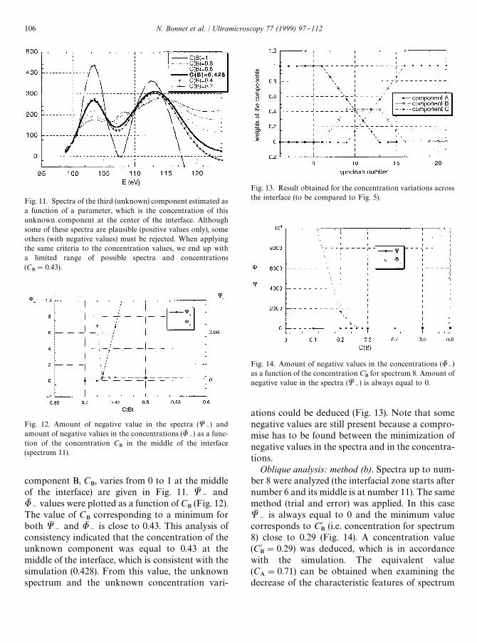
Fig. 11. Spectra of the third (unknown) component estimated asa function of a parameter, which is the concentration of thisunknown component at the center of the interface. Althoughsome of these spectra are plausible (positive values only), someothers (with negative values) must be rejected. When applyingthe same criteria to the concentration values, we end up witha limited range of possible spectra and concentrations(C

B"0.43).

Fig. 12. Amount of negative value in the spectra (WM~) and

amount of negative values in the concentrations (UM~) as a func-

tion of the concentration CB

in the middle of the interface(spectrum 11).

component B, CB, varies from 0 to 1 at the middle

of the interface) are given in Fig. 11. WM~

andUM

~values were plotted as a function of C

B(Fig. 12).

The value of CB

corresponding to a minimum forboth WM

~and UM

~is close to 0.43. This analysis of

consistency indicated that the concentration of theunknown component was equal to 0.43 at themiddle of the interface, which is consistent with thesimulation (0.428). From this value, the unknownspectrum and the unknown concentration vari-

Fig. 13. Result obtained for the concentration variations acrossthe interface (to be compared to Fig. 5).

Fig. 14. Amount of negative values in the concentrations (UM~)

as a function of the concentration C@B

for spectrum 8. Amount ofnegative value in the spectra (WM

~) is always equal to 0.

ations could be deduced (Fig. 13). Note that somenegative values are still present because a compro-mise has to be found between the minimization ofnegative values in the spectra and in the concentra-tions.

Oblique analysis: method (b). Spectra up to num-ber 8 were analyzed (the interfacial zone starts afternumber 6 and its middle is at number 11). The samemethod (trial and error) was applied. In this caseWM

~is always equal to 0 and the minimum value

corresponds to C@B

(i.e. concentration for spectrum8) close to 0.29 (Fig. 14). A concentration value(C@

B"0.29) was deduced, which is in accordance

with the simulation. The equivalent value(C

A"0.71) can be obtained when examining the

decrease of the characteristic features of spectrum


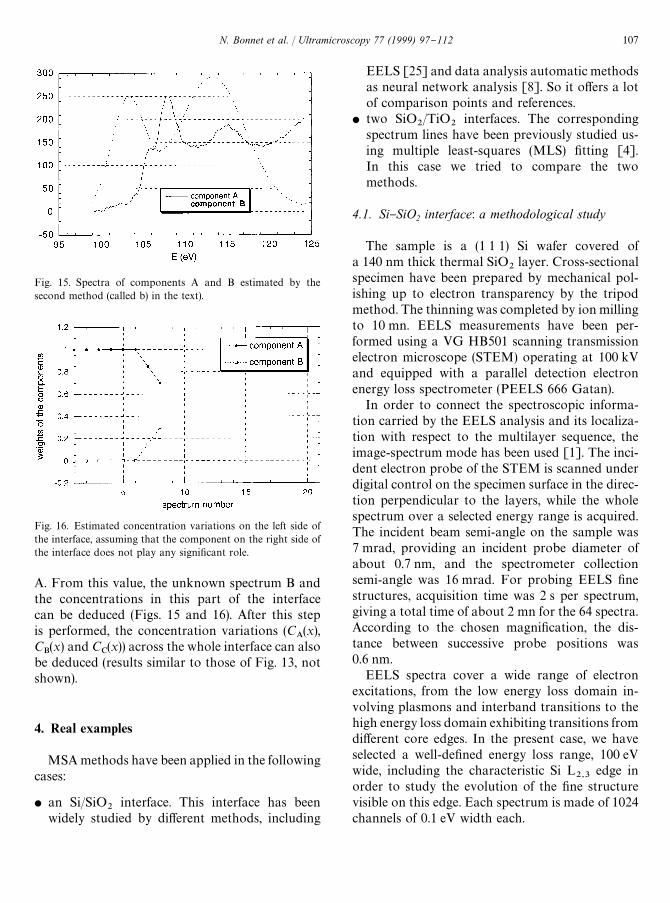
Fig. 15. Spectra of components A and B estimated by thesecond method (called b) in the text).

Fig. 16. Estimated concentration variations on the left side ofthe interface, assuming that the component on the right side ofthe interface does not play any signi"cant role.

A. From this value, the unknown spectrum B andthe concentrations in this part of the interfacecan be deduced (Figs. 15 and 16). After this stepis performed, the concentration variations (C

A(x),

CB(x) and C

C(x)) across the whole interface can also

be deduced (results similar to those of Fig. 13, notshown).

4. Real examples

MSA methods have been applied in the followingcases:

f an Si/SiO2

interface. This interface has beenwidely studied by di!erent methods, including

EELS [25] and data analysis automatic methodsas neural network analysis [8]. So it o!ers a lotof comparison points and references.

f two SiO2/TiO

2interfaces. The corresponding

spectrum lines have been previously studied us-ing multiple least-squares (MLS) "tting [4].In this case we tried to compare the twomethods.

4.1. Si}SiO2 interface: a methodological study

The sample is a (1 1 1) Si wafer covered ofa 140 nm thick thermal SiO

2layer. Cross-sectional

specimen have been prepared by mechanical pol-ishing up to electron transparency by the tripodmethod. The thinning was completed by ion millingto 10 mn. EELS measurements have been per-formed using a VG HB501 scanning transmissionelectron microscope (STEM) operating at 100 kVand equipped with a parallel detection electronenergy loss spectrometer (PEELS 666 Gatan).

In order to connect the spectroscopic informa-tion carried by the EELS analysis and its localiza-tion with respect to the multilayer sequence, theimage-spectrum mode has been used [1]. The inci-dent electron probe of the STEM is scanned underdigital control on the specimen surface in the direc-tion perpendicular to the layers, while the wholespectrum over a selected energy range is acquired.The incident beam semi-angle on the sample was7 mrad, providing an incident probe diameter ofabout 0.7 nm, and the spectrometer collectionsemi-angle was 16 mrad. For probing EELS "nestructures, acquisition time was 2 s per spectrum,giving a total time of about 2 mn for the 64 spectra.According to the chosen magni"cation, the dis-tance between successive probe positions was0.6 nm.

EELS spectra cover a wide range of electronexcitations, from the low energy loss domain in-volving plasmons and interband transitions to thehigh energy loss domain exhibiting transitions fromdi!erent core edges. In the present case, we haveselected a well-de"ned energy loss range, 100 eVwide, including the characteristic Si L

2,3edge in

order to study the evolution of the "ne structurevisible on this edge. Each spectrum is made of 1024channels of 0.1 eV width each.


Fig. 17. Residual images of the Si/SiO2

interface, i. e. di!erence between original and reconstituted spectra. Each spectrum constitutesone line of each image, grey levels being proportional to the spectrum di!erence intensity.

Fig. 1 shows the whole set of data acquired ina spectrum-line made of 64 spectra collected acrossthe Si/SiO

2interface. In the crystalline Si part, the

Si L2,3

edge onset is at 99.8 eV [25], whereas theSiO

2spectrum is characterized by 3 main absorp-

tion features at 106, 108 and 115 eV. Most of theresults concerning Si/SiO

2interface conclude to the

presence of an SiOxsuboxide layer, as well by XPS

[26] as by EELS [25,27]. The aim of this part of thestudy is to check whether it is possible to extract thecontribution of SiO

xto the EELS spectrum by

using MSA.We have chosen to analyze spectra nos. 23}35

over an energy window from 98 to 125 eV, wherethe signi"cative features are situated. The in#uenceof multiple scattering events varying with probe

position, could introduce aliasing contribution atabout 20 eV above threshold. However, as demon-strated in the present analysis (see Fig. 17), alldeviations between experimental and modelled-spectra are only important over the "rst 10 eV atthreshold. Consequently we can estimate that insuch a practical case, the in#uence of variablemultiple scattering remains negligible. As it hasbeen explained in Section 3.2, "rst we have todetermine how many components are present ina series of spectra. The factor indicator function ofMalinowski has its minimum value for 3 compo-nents (Table 1), moreover, the Akaike criterionhas its minimum value for 4 components; as thetrue number of components is often less by one,these 2 criteria agree to conclude that there are 3


Table 1

Number of axes/criterium 2 3 4 5 6

Malinowski 0.00094 0.00081 0.00083 0.00096 0.00117Akaike 112.3 105.7 103.4 103.8 104.7

components. A third indicator is given by the in-spection of residual images in Fig. 17. On the imagereconstituted with 2 axes it is clearly visible thatthere is a bad reconstitution appearing as black andwhite spots located precisely in the interface region.These errors are greatly attenuated in the imagereconstituted with 3 components. Once the exist-ence of the component B has been assessed, we haveto perform an oblique analysis in order to "nd a setof reference spectra having a physical meaning.

We have used the "rst method presented in Sec-tion 3.3 by letting the concentration of the un-known component (SiO

x) vary. Then criteria to

choose the `righta concentration are:

f the positiveness of concentrations for all ana-lyzed points,

f the positiveness of intensity for the third obliquespectrum.

In Fig. 18 are displayed values representing `nega-tivea concentrations (WM

~) and `negativea inten-

sities (UM~).

We see that minimum values for the two indi-cators are obtained for C"0.5. Corresponding

Fig. 18. Values representing `negativea concentrations (WM~)

and negative intensities (UM~

) as a function of the concentrationof the unknown component.

Fig. 19. Spectra of the "rst, second and third components. The"rst and third components (SiO

2and Si) were picked out far

from the interface and the second component was deducedaccording to the oblique analysis (variant a).

Fig. 20. Estimated concentration pro"les corresponding to the3 components.

spectra are presented in Fig. 19 and pro"les in Fig.20. It is interesting to compare the third component(B) with EELS spectra obtained on suboxide sam-ples [28]. Di!erent silicon environments (fromSiSi

4, a silicon atom surrounded by 4 silicon atoms,


Fig. 21. Residual images of the two SiO2/TiO

2interfaces, for a reconstitution with two and three factorial axes. For both cases, the

grey-level dynamic is maintained when displaying the residual images. For interface A, the reconstitution with two axes is su$cient (noimportant contrast is visible) and it is not improved when adding another factorial axis. For interface B, the reconstitution with two axesis insu$cient (a marked contrast is visible in the interface region). It is greatly improved when considering a third factorial axis.

to SiO4, a silicon atom surrounded by 4 oxygen

atoms) probably give rise to a shift in the Si edge.The broad and smooth edge may thus be due tocontributions from partially oxidized silicon.

4.2. SiO2}TiO2: comparison between two interfaceswith and without a third phase

The sample is an SiO2}TiO

2multilayers se-

quence used in optical coatings. Two line spectraacquired on di!erent interfaces have already beenstudied using the MLS "tting technique [4]. One ofthem is displayed in Fig. 2. Results show that for

one of the interfaces, some of the spectra located atthe interface exhibit features characteristically dif-ferent from a linear combination of the two refer-ences recorded on each side of the interface.

We have used MSA in order to extract the speci-"c component of the interface phase, and to checkthat it is present in one of the line spectra only. Inthis case we have focused our study on O K edge at532 eV which is present on both sides of the inter-face, and whose "ne structures change signi"cantlydepending on whether it is due to TiO

2or SiO

2.

For the line-spectrum A, we have used spectra nos.21}41 over an energy window between 525 and


550 eV; for the line-spectrum B the window wasslightly larger (spectra nos. 10}50, energy between520 and 573 eV). For these spectra the most evidentcriteria to determine the number of relevant com-ponents is the visual examination of residual im-ages (Fig. 21). For the interface B, there is a strongdiscrepancy for reconstruction with 2 axes only,whereas the use of a third axis signi"cantly im-proves the reconstruction. On the contrary for theinterface A the reconstruction with 2 axes seemsalready satisfactory and indeed the third axis doesnot signi"cantly modify the remaining noise. Forthe interface A the oblique analysis is straightfor-ward and Fig. 22 shows the corresponding pro"les.They are of course quite similar to those obtainedby MLS techniques.

Fig. 22. Estimated concentration pro"les corresponding to twocomponents, A and C, for interface A.

Fig. 23. Spectra of the three components for interface B. The"rst and third components (SiO

2and TiO

2) were picked out far

from the interface and the second component was deducedaccording to the oblique analysis (variant a).

Fig. 24. Estimated concentration pro"les corresponding to3 components for interface B.

In the case of the interface B, the same method asfor the Si}SiO

2interface has been applied. The

weight of the third component has been foundequal to 0.4. The corresponding spectrum is shownin Fig. 23 and the pro"les in Fig. 24.

The third component is not much di!erent fromthose of O K in SiO

2, which could explain that its

pro"le extends widely in the SiO2

side. Indeed thiscomponent can be compared to the spectrum ob-tained on a sample of SiO

2}TiO

2glass. It could be

related to an oxygen atom surrounded by both Siand Ti atoms.

5. Conclusions

In the study of an interface, it is important todiscriminate the "ne structures relative to theatoms at the interface from those corresponding tothe surrounding matrix. MSA constitutes an un-biased tool for the search of such components fromwhich we can deduce the associated compositionalpro"les.

Compared to more conventional data analysisprocedures, such as MLS, MSA has the advantageof o!ering more tools for estimating the number ofcomponents present at the interface. When a thirdcomponent is present (in addition to the compo-nents present far from the interface), MSA alsoallows to estimate the spectrum of this componentand the concentration variations across theinterface.


Although a detailed comparative study remainsto be done, we consider that the results provided byMSA can be obtained more simply than those ofneural networks of the adaptive resonance theory(ART)-type. In the next stage, once intermediate"ne structures patterns have been identi"ed, onehas to relate them to the local atomic environmentand local structure, which will require more exten-sive theoretical calculations for modelling these "nestructures.

Acknowledgements

We thank, K. Yu-Zhang (UniversiteH de Marne laValleH e, France) and J. Rivory (UniversiteH Paris VI,France) for supplying the sample.

References

[1] C. Colliex, M. TenceH , E. Lefevre, C. Mory, H. Gu,D. Bouchet, C. Jeanguillaume, Mikrochim. Acta 114/115(1994) 71.

[2] M. TenceH , M. Quartuccio, C. Colliex, Ultramicroscopy 58(1995) 42.

[3] J. Bruley, M.-W. Tseng, D.B. Williams, Microsc. Micro-anal. Microstruct. 6 (1995) 1.

[4] N. Brun, C. Colliex, J. Rivory, K. Yu-Zhang, Microsc.Microanal. Microstruct. 7 (1996) 161.

[5] H. MuK llejans, J. Bruley, Ultramicroscopy 53 (1994) 351.[6] H. MuK llejans, J. Bruley, J. Microsc. 180 (1995) 12.

[7] H. Gu, M. Ceh, S. Stemmer, H. MuK llejans, M. RuK hle,Ultramicroscopy 59 (1995) 215.

[8] C. Gatts, G. Duscher, H. MuK llejans, M. RuK hle, Ultramic-roscopy 59 (1995) 229.

[9] P. Moreau, N. Brun, C.A. Walsh, C. Colliex, A. Howie,Phys. Rev. B 56 (1997) 6774.

[10] P. Trebbia, N. Bonnet, Ultramicroscopy 34 (1990) 165.[11] P. Trebbia, C. Mory, Ultramicroscopy 34 (1990) 179.[12] I.M. Anderson, J. Bentley. Proc. Microsc. Microanal. 1997

(1997) 931[13] P.M. Rice, K.B. Alexander, I.M. Anderson, Proc. Microsc.

Microanal. 1997 (1997) 945.[14] N. Bonnet, E. Simova, X. Thomas, Microsc. Microanal.

Microstruct. 2 (1991) 129.[15] M. Titchmarsh, S. Dumbill, J. Microsc. 184 (3) (1996)

195.[16] M. Titchmarsh, S. Dumbill, J. Microsc. 188 (1997) 224.[17] E. Malinowsky, D. Howery, Factor Analysis in Chemistry,

Wiley Interscience, New York, 1980.[18] H. Akaike, IEEE Trans. Automat. Control 19 (1974) 716.[19] J.P. Bretaudiere, J. Frank, J. Microsc. 144 (1986) 1.[20] S. GarenstroK m, Appl. Surf. Sci. 7 (1981) 7.[21] S. GarenstroK m, Appl. Surf. Sci. 26 (1986) 561.[22] C. Palacio, H.J. Mathieu, Surf. Interface Anal. 16 (1990)

178.[23] M. Sarkar, L. Calliari, L. Gonzo, F. Marchetti, Surf. Inter-

face Anal. 20 (1993) 60.[24] R. Vidal, J. Ferron, Appl. Surf. Sci. 31 (1988) 263.[25] P.E. Batson, Nature 366 (1993) 727.[26] F.J. Himpsel, F.R. McFeely, A. Taleb-Ibrahimi, J.A. Yar-

mo!, Phys. Rev. B 38 (1988) 6084.[27] G. Duscher, Oxidische Korngrenzenphasen im Silicium,

Dissertation, University of Stuttgart, 1996.[28] D. J. Wallis, Structure of amorphous oxides and nitrides

of silicon, Ph.D. Dissertation, University of Cambridge,1994.


extracting information from sequences of spatially...

Documents