extending encog: a study on classiﬁer ensemble techniquesamosca02/pdfs/msc_thesis_final.pdf ·...

Extending Encog: a study on classifier ensemble

techniques

Alan Mosca

MSc Computer Science Project Report

Department of Computer Science and Information Systems

Birkbeck College, University of London

September 2012

Abstract

The goal of this project is to illustrate the creation of additional components forthe Encog Java Library, which implement some of the most common and widelyused ensemble learning techniques. I will cover the prior knowledge requiredfor understanding the work, including mathematical proof and discussion wherepossible, the design of the new components and how they fit in the overall designof the library, the procedure of validating and evaluating the performance of thenewly implemented techniques, and finally the results of this evaluation.

Supervisor: Dr G. Magoulas

i

Contents

Abstract i

Contents iv

1 Introduction 2

1.1 Purpose of the project . . . . . . . . . . . . . . . . . . . . . . . . 21.2 Background . . . . . . . . . . . . . . . . . . . . . . . . . . . . . . 2

1.2.1 Machine learning problems . . . . . . . . . . . . . . . . . 31.2.2 Online vs Offline learning . . . . . . . . . . . . . . . . . . 41.2.3 Ensemble Learning . . . . . . . . . . . . . . . . . . . . . . 4

1.3 Approach . . . . . . . . . . . . . . . . . . . . . . . . . . . . . . . 41.4 Structure of this document . . . . . . . . . . . . . . . . . . . . . 4

1.4.1 Review . . . . . . . . . . . . . . . . . . . . . . . . . . . . 41.4.2 Implementation . . . . . . . . . . . . . . . . . . . . . . . . 51.4.3 Benchmarking . . . . . . . . . . . . . . . . . . . . . . . . 51.4.4 Conclusions . . . . . . . . . . . . . . . . . . . . . . . . . . 5

2 Using Artificial Neural Networks as classifiers 6

2.1 The basic neuron . . . . . . . . . . . . . . . . . . . . . . . . . . . 72.2 Networks . . . . . . . . . . . . . . . . . . . . . . . . . . . . . . . 8

2.2.1 Classification output . . . . . . . . . . . . . . . . . . . . . 82.2.2 Cost function / Training Error . . . . . . . . . . . . . . . 82.2.3 Training and initialization . . . . . . . . . . . . . . . . . . 9

2.3 Performance . . . . . . . . . . . . . . . . . . . . . . . . . . . . . . 92.3.1 Classification Error . . . . . . . . . . . . . . . . . . . . . . 102.3.2 Misclassification . . . . . . . . . . . . . . . . . . . . . . . 102.3.3 Accuracy . . . . . . . . . . . . . . . . . . . . . . . . . . . 102.3.4 Precision and Recall . . . . . . . . . . . . . . . . . . . . . 102.3.5 F1-score . . . . . . . . . . . . . . . . . . . . . . . . . . . . 112.3.6 Bias and Variance . . . . . . . . . . . . . . . . . . . . . . 11

2.4 Weak learners . . . . . . . . . . . . . . . . . . . . . . . . . . . . . 11

3 Ensembles 12

3.1 History . . . . . . . . . . . . . . . . . . . . . . . . . . . . . . . . 123.2 Overview . . . . . . . . . . . . . . . . . . . . . . . . . . . . . . . 133.3 Training set diversity . . . . . . . . . . . . . . . . . . . . . . . . . 13

3.3.1 Introduction of noise . . . . . . . . . . . . . . . . . . . . . 133.3.2 Bagging . . . . . . . . . . . . . . . . . . . . . . . . . . . . 14

ii

3.3.3 Boosting . . . . . . . . . . . . . . . . . . . . . . . . . . . . 143.4 Architectural diversity . . . . . . . . . . . . . . . . . . . . . . . . 14

3.4.1 Diverse Neural Groups . . . . . . . . . . . . . . . . . . . . 143.5 Combining outputs . . . . . . . . . . . . . . . . . . . . . . . . . . 15

3.5.1 Averaging . . . . . . . . . . . . . . . . . . . . . . . . . . . 153.5.2 Majority voting . . . . . . . . . . . . . . . . . . . . . . . . 163.5.3 Stacking . . . . . . . . . . . . . . . . . . . . . . . . . . . . 163.5.4 Ranking . . . . . . . . . . . . . . . . . . . . . . . . . . . . 16

4 The Encog Library 17

4.1 Architecture . . . . . . . . . . . . . . . . . . . . . . . . . . . . . . 174.1.1 Machine Learning Packages . . . . . . . . . . . . . . . . . 174.1.2 Neural Network Packages . . . . . . . . . . . . . . . . . . 184.1.3 Activation Functions . . . . . . . . . . . . . . . . . . . . . 214.1.4 Utility Packages . . . . . . . . . . . . . . . . . . . . . . . 22

5 Implementation 23

5.1 Layout of the project . . . . . . . . . . . . . . . . . . . . . . . . . 235.1.1 Packages . . . . . . . . . . . . . . . . . . . . . . . . . . . . 23

5.2 Adding features to Encog . . . . . . . . . . . . . . . . . . . . . . 245.2.1 Design decisions . . . . . . . . . . . . . . . . . . . . . . . 245.2.2 Architectural changes . . . . . . . . . . . . . . . . . . . . 245.2.3 Class design model . . . . . . . . . . . . . . . . . . . . . . 24

5.3 Creating a framework for testing . . . . . . . . . . . . . . . . . . 275.4 Source management . . . . . . . . . . . . . . . . . . . . . . . . . 27

5.4.1 Revision control . . . . . . . . . . . . . . . . . . . . . . . 275.4.2 Automated building . . . . . . . . . . . . . . . . . . . . . 28

6 Benchmarking the new features 29

6.1 Running tests . . . . . . . . . . . . . . . . . . . . . . . . . . . . . 296.1.1 The test plan . . . . . . . . . . . . . . . . . . . . . . . . . 296.1.2 The test program . . . . . . . . . . . . . . . . . . . . . . . 29

6.2 Infrastructure layout . . . . . . . . . . . . . . . . . . . . . . . . . 316.2.1 The PBS system . . . . . . . . . . . . . . . . . . . . . . . 316.2.2 AWS compute nodes . . . . . . . . . . . . . . . . . . . . . 316.2.3 Submission tools . . . . . . . . . . . . . . . . . . . . . . . 326.2.4 Aggregating results . . . . . . . . . . . . . . . . . . . . . . 326.2.5 Creating graphs and tables . . . . . . . . . . . . . . . . . 32

6.3 The data sets . . . . . . . . . . . . . . . . . . . . . . . . . . . . . 326.3.1 Haberman’s Survival . . . . . . . . . . . . . . . . . . . . . 336.3.2 Letter Recognition . . . . . . . . . . . . . . . . . . . . . . 336.3.3 Landsat . . . . . . . . . . . . . . . . . . . . . . . . . . . . 336.3.4 Magic . . . . . . . . . . . . . . . . . . . . . . . . . . . . . 34

6.4 Reducing the search space . . . . . . . . . . . . . . . . . . . . . . 346.4.1 Previous literature . . . . . . . . . . . . . . . . . . . . . . 346.4.2 Picking parameters . . . . . . . . . . . . . . . . . . . . . . 346.4.3 Training Curves and Final Parameters . . . . . . . . . . . 366.4.4 Dividing ranges . . . . . . . . . . . . . . . . . . . . . . . . 45

iii

7 Test results 46

7.1 Bagging . . . . . . . . . . . . . . . . . . . . . . . . . . . . . . . . 477.1.1 Majority voting . . . . . . . . . . . . . . . . . . . . . . . . 477.1.2 Averaging . . . . . . . . . . . . . . . . . . . . . . . . . . . 55

7.2 AdaBoost . . . . . . . . . . . . . . . . . . . . . . . . . . . . . . . 627.2.1 Majority voting . . . . . . . . . . . . . . . . . . . . . . . . 627.2.2 Averaging . . . . . . . . . . . . . . . . . . . . . . . . . . . 70

7.3 Stacking . . . . . . . . . . . . . . . . . . . . . . . . . . . . . . . . 757.3.1 MetaClassifier . . . . . . . . . . . . . . . . . . . . . . . . . 75

8 Discussion, Conclusions and Further Work 78

8.1 Validity of results . . . . . . . . . . . . . . . . . . . . . . . . . . . 788.2 Efficiency . . . . . . . . . . . . . . . . . . . . . . . . . . . . . . . 788.3 Noise . . . . . . . . . . . . . . . . . . . . . . . . . . . . . . . . . . 788.4 Different datasets have different results . . . . . . . . . . . . . . . 798.5 Further work . . . . . . . . . . . . . . . . . . . . . . . . . . . . . 79

8.5.1 Re-running benchmarks with different parameters . . . . 798.5.2 Further expansions to Encog . . . . . . . . . . . . . . . . 798.5.3 Contribution back to the community . . . . . . . . . . . . 798.5.4 Real-world use of Encog Ensembles . . . . . . . . . . . . . 80

iv

List of Figures

2.1 The sigmoid activation function . . . . . . . . . . . . . . . . . . . 7

4.1 Basic encog ML package . . . . . . . . . . . . . . . . . . . . . . . 184.2 Common NN classes and interfaces in org.encog.neural . . . . . . 194.3 NN architecture related classes and interfaces in org.encog.neural 204.4 NN training interfaces and classes in org.encog.neural . . . . . . 214.5 NN activation functions . . . . . . . . . . . . . . . . . . . . . . . 22

5.1 Class diagram of added components . . . . . . . . . . . . . . . . 27

6.1 Training and test error for Haberman with 30 neurons . . . . . . 366.2 Training and test error for Haberman with 100 neurons . . . . . 376.3 Training and test error for Haberman with 300 neurons . . . . . 376.4 Training and test error for Letter Recognition with 30 neurons . 386.5 Training and test error for Letter Recognition with 100 neurons . 396.6 Training and test error for Letter Recognition with 300 neurons . 396.7 Training and test error for Landsat with 30 neurons . . . . . . . 406.8 Training and test error for Landsat with 100 neurons . . . . . . . 416.9 Training and test error for Landsat with 300 neurons . . . . . . . 416.10 Training and test error for Magic with 30 neurons . . . . . . . . 426.11 Training and test error for Magic with 100 neurons . . . . . . . . 436.12 Training and test error for Magic with 300 neurons . . . . . . . . 44

7.1 Performance on the Haberman dataset (test set) for Bagging with Majority Voting 487.2 Performance on the Haberman dataset (training set) for Bagging with Majority Voting 497.3 Class bias on the Haberman dataset (test set) for Bagging with Majority Voting 497.4 Performance on the Letter Recognition dataset (test set) for Bagging with Majority Voting 507.5 Performance on the Letter Recognition dataset (training set) for Bagging with Majority Voting 517.6 Class bias on the Letter Recognition dataset (test set) for Bagging with Majority Voting 517.7 Performance on the Landsat dataset (test set) for Bagging with Majority Voting 527.8 Performance on the Landsat dataset (training set) for Bagging with Majority Voting 537.9 Class bias on the Landsat dataset (test set) for Bagging with Majority Voting 537.10 Performance on the Magic dataset (test set) for Bagging with Majority Voting 547.11 Performance on the Magic dataset (training set) for Bagging with Majority Voting 557.12 Class bias on the Magic dataset (test set) for Bagging with Majority Voting 557.13 Class bias on the Magic dataset (training set) for Bagging with Majority Voting 557.14 Performance on the Haberman dataset (test set) for Bagging with Averaging 577.15 Performance on the Haberman dataset (training set) for Bagging with Averaging 577.16 Class bias on the Haberman dataset (test set) for Bagging with Averaging 57

v

7.17 Performance on the Letter Recognition dataset (test set) for Bagging with Averaging 587.18 Performance on the Letter Recognition dataset (training set) for Bagging with Averaging 597.19 Class bias on the Letter Recognition dataset (test set) for Bagging with Averaging 597.20 Performance on the Magic dataset (test set) for Bagging with Averaging 607.21 Performance on the Magic dataset (training set) for Bagging with Averaging 617.22 Class bias on the Magic dataset (test set) for Bagging with Averaging 617.23 Class bias on the Magic dataset (training set) for Bagging with Averaging 617.24 Performance on the Haberman dataset (test set) for Bagging with Majority Voting 637.25 Performance on the Haberman dataset (training set) for Bagging with Majority Voting 637.26 Class bias on the Haberman dataset (test set) for Bagging with Majority Voting 637.27 Performance on the Letter Recognition dataset (test set) for Bagging with Majority Voting 657.28 Performance on the Letter Recognition dataset (training set) for Bagging with Majority Voting 657.29 Class bias on the Letter Recognition dataset (test set) for Bagging with Majority Voting 657.30 Performance on the Landsat dataset (test set) for Bagging with Majority Voting 677.31 Performance on the Landsat dataset (training set) for Bagging with Majority Voting 677.32 Class bias on the Landsat dataset (test set) for Bagging with Majority Voting 677.33 Performance on the Magic dataset (test set) for Bagging with Majority Voting 687.34 Performance on the Magic dataset (training set) for Bagging with Majority Voting 69

vi

List of Tables

7.1 Performance for the haberman dataset (bagging - majorityvoting) 487.2 Performance for the letterrecognition dataset (bagging - majorityvoting) 507.3 Performance for the landsat dataset (bagging - majorityvoting) . 527.4 Performance for the magic dataset (bagging - majorityvoting) . . 547.5 Performance for the haberman dataset (bagging - averaging) . . 567.6 Performance for the letterrecognition dataset (bagging - averaging) 587.7 Performance for the magic dataset (bagging - averaging) . . . . . 607.8 Performance for the haberman dataset (adaboost - majorityvoting) 627.9 Performance for the letterrecognition dataset (adaboost - majorityvoting) 647.10 Performance for the landsat dataset (adaboost - majorityvoting) 667.11 Performance for the magic dataset (adaboost - majorityvoting) . 687.12 Performance for the haberman dataset (adaboost - averaging) . . 707.13 Performance for the letterrecognition dataset (adaboost - averaging) 717.14 Performance for the landsat dataset (adaboost - averaging) . . . 737.15 Performance for the landsat dataset (stacking - metaclassifier-mlp30-0.07) 757.16 Performance for the letterrecognition dataset (stacking - metaclassifier-mlp100-0.02) 767.17 Performance for the landsat dataset (stacking - metaclassifier-mlp30-0.07) 77

1

Chapter 1

Introduction

Ensemble learning techniques are a very powerful tool in Machine Learning.They have proven themselves time and time again to be useful for improving theperformance of machine learning techniques, and can be applied to an existingprocess without changing the understanding of the problem too much. Thus,they have been recently used to a very large extent (the top two entries of thenetflix million dollar prize were both implementations of stacked generalization- a very common and powerful ensemble technique). In parallel, there is a well-known Java library called Encog, which implements many machine learningtechniques and has reached a good level of adoption. This library is, however,missing Ensemble techniques in its current implementation, and there have beenseveral requests to add such functionality to the library.

1.1 Purpose of the project

The plan for this project was to implement the support for ensemble techniquesinto Encog, and to add a few of the common methodologies. As well as a de-sign and coding exercise, it is an exploration of the various ensemble techniquesavailable. I also planned to test the performance using some of the readily avail-able datasets and to compare the results to some others already published. Thenumber of machine learning techniques, ensemble techniques and test datasetsis very large, so during implementation it was only realistically possible to at-tack a subset of the possibilities in this project. Having to choose, I pickedNeural Networks as the underlying machine learning techniques because Encogwas initially born as a Neural Networks package and subsequently expanded.

1.2 Background

There is a lot of literature on machine learning methods in general and onneural networks in particular, and on ensemble learning methods. The relevantchapters will cover the prior work more in detail.

2

1.2.1 Machine learning problems

Machine learning techniques are varied and can be applied to many differenttypes of problems. These problems are normally categorised by lerning methodand by output type.

Supervised learning

Supervised learning is a method of learning where a training set is providedalong with the expected output for each element of the training set, such thatthe learning algorithm can generate a system that will perform predictions onnew sets presented at a later date. A test set is also provided with similarcharacteristics (but with independent data from the training set), so that it ispossible to compare the predicted outputs with the correct ones, and approx-imate the level of error of a certain algorhithm. Another sub-classification ismade based on the type of prediction:

• Classification problems. With classification problems, we are presentedwith a number of input attributes and we are expected to predict which”class” these inputs belong to. This is a powerful technique for patternrecognition and decision making.

• Regression problems. Regression problems still make predictions, butrather than predicting that a set belongs to a certain class, they predictan unbounded output value. This is a poweful technique for predictingopen-ended data, like prices or rainfall (and many others).

Many of the supervised learning techniques can be used both for classificationand regression, with only very small adaptations.

Unsupervised learning

Unsupervised learning techniques are generally presented with a set of data thatdo not have any associated prior results (this is often referred to as unlabeleddata). The machine learning algorithm is expected to produce output (e.g.classification) solely based on patters from the input data.

• Clustering. Clustering is an unsupervised technique used to extract classvalues from the way that the data tends to cluster around certain values.There are several different techniques, but most of them tend to make atleast some assumption about the output that is expected (e.g. the numberof classes).

• Generative models. Generative models are used in machine learning tosimulate the distribution of a variable. These technique will ”learn” adistribution and produce (generate) new samples according to this internalmodel.

• Dimensionality reduction. Dimensionality reduction can be defined as amethod that reduces the number of features in a specific data set, withthe intent of improving performance and accuracy of a machine learningmethod. This can be done either by feature selection, which tries to dis-card some features that may not be very significant (or indeed just noise),

3

and feature extraction, which tries to combine the information containedin two or more features, into a smaller number of features without losingdata.

1.2.2 Online vs Offline learning

We can decide to train our machine learning systems once before using them(offline learning), or we can feed back the information from inputs that arrivewhile predictions are being made (online learning). This second technique re-quires some way of providing feedback to the system, and the training methodsneed to be adapted so that the system is updated quickly enough so as to notaffect the performance by too much.

1.2.3 Ensemble Learning

Ensemble learning combines many different learning techniques in order to im-prove the proficiency of predictions, and is the main focus of this paper. Ifapplied correctly it is a very powerful approach and can improve machine learn-ing systems that were previously considered unusable to the point that they arewidely adopted. There are several techniques and they will all be covered intheir own chapter.

1.3 Approach

The project can be divided in different focus areas:

1. The first part of the project focused on implementing the support forensemble techniques in Encog, trying to alter the original structure of thelibrary as little as possible. This will enable other contributors to add newensemble techniques easily following an agreeable standard.

2. To implement some of the most common techniques and methods on topof this basic framework design, with the dual purpose of testing the frame-work and providing working examples.

3. The creation of a benchmarking environment, including the support forrunning long jobs. This is an essential part of the implementation, becauseit will provide immediate feedback on the performance of the library

4. Investigation of some datasets for benchmarking. We require some well-known data to assess correctness of the techniques and also provide acomparison between each approach.

5. Benchmarking is the last part of the project, and its success depends onall the other tasks being completed correctly and efficiently.

1.4 Structure of this document

1.4.1 Review

In the first two chapters I explore more in detail the existing knowledge andliteratrue, and present some of the most common approaches. Chapter two

4

explores Neural Networks and classification problems and gives an overviewof the current techniques. The third chapter gives an overview of both thehistory of ensemble learning and the current most known approaches. Thefourth chapter explains some of the internal architecture of the Encog libraryand looks for potential ways of implementing new features in a low-disruptionfashion.

1.4.2 Implementation

Chapter 5 will cover the changes to the library, with an explanation of thearchitecture of the new components, and how they interact with the pre-existingcode.

1.4.3 Benchmarking

The first part of chapter 6 is about the architecture of the benchmark system,and all the support infrastructure for running benchmark jobs. The secondpart focuses on selecting the right datasets and parameters, and providing acomparison for how single Neural Network perform on these datasets. Chapter7 presents the results for all the various benchmarks on each of the implementedtechniques, with a commentary on the observed features of these results.

1.4.4 Conclusions

Chapter 8 looks at the evidence presented in the previous chapters and drawsconclusions on these ensemble techniques and their implementation, and presentssome of the possibilities for expansion and revision of this work.

5

Chapter 2

Using Artificial NeuralNetworks as classifiers

This chapter covers the basics of the underlying techniques of neural networks.For a deeper discussion of the subject, please refer to the vast literature on thesubject, for example [3, 38]. Neural networks are just one of many machinelearning algorithms that implement classifiers. Over time many different typesof neural networks have been developed and evolved, with varied architecture,function, scope and performance.

Notation In this chapter I use some notation conventions, which are explainedalong in the chapter. I include a quick reference table here for convenience:

• X: a vector of inputs

• W : the weights vector characteristic of a neuron

• n: the number of input values, or the dimensionality of X and W

• f(X): the function implemented by a neural network

• y: the output of a neuron

• t: the weighted sum of the inputs of a neuron

• A(t): the activation function of a neuron

• P (t): the logistic function P (t) = 1

1+e−t

• Y : a vector of outputs

• z: the number of output values, or the dimensionality of Y

• C(Y ): the classification function

• c(y): the output rounding function for classification

• Y ′: the vector of classification decisions

• fc(X): the function implemented by a classifier

• m: the number of instances in a data set

6

2.1 The basic neuron

Virtually all neural networks are based on an elementary component, the neuron.The simple artificial neuron is modelled around the behaviour of the biologicalneuron, found in the brains of humans (and animals). The neuron has fewfundamental characteristics:

• A vector of n inputs X ∈ Rn0..1

• A vector of numerical weights W ∈ Rn, each associated with an input

• An output y ∈ R0..1

If we call xi the ith input, wi the associated weight for that input and n thenumber of inputs of the neuron, we can say that most neurons will implementthe function

y = A(n∑

i=1

wixi)

1 where A(t) ∈ R → R0..1 is the activation function of the neural network. Avery common activation function is the sigmoid activation function:

P (t) =1

1 + e−t

0

0.1

0.2

0.3

0.4

0.5

0.6

0.7

0.8

0.9

1

-10 -5 0 5 10

1 / ( 1 + ( exp (-x) ) )0.5

Figure 2.1: The sigmoid activation function

Applying this function to the sum of the weighted inputs puts the output inthe correct range (0..1), allowing us to use the output of one neuron as the inputto another. This is the basic building element for constructing neural networks.2

1We could vectorize this with a weight vector W and an input vector X and obtain thesimpler notation P (WX′). This is common practice in Machine Learning notation, both forsimplicity reasons and because many implementations are vectorized to optimize for speed.[37]

2There are some variants of Neurons that use the range [ -1 .. 1 ] instead of [ 0 .. 1 ] inboth the inputs and the output. This can be considered to be equivalent from a functionalperspective and is mostly just a matter of preference.

7

2.2 Networks

The fact that the output of a Neuron is designed to be in the same range ofits inputs, makes it easy to build networks of many neurons with very diversetopologies and characteristics:

• The multilayer perceptron

• Recurrent networks: hopfield, boltzmann, hierarchical, long short termmemory networks ...

• Self-organizing networks (e.g. Kohonen)

The in-depth description of these and other techniques goes beyond the scopeof this document, and can be easily found in [3, 5, 4] or other textbooks onthe subject of ANNs. As a generalization, it can be said that any ANN willimplement a function f(X) ∈ R

n→ R

z on the input vector X ∈ Rn.

2.2.1 Classification output

One vs All method

In order to categorize the input data into multiple distinct classes, the mostcommon solution is to use multiple binary outputs Y ′

∈ Rz0..1 - one for each

class - and to ”select” the class with the highest output as the classificationoutput.

Classification function

The classification function can be defined as fc(X) ∈ Rn0..1 → R

z0..1 or fc(X) ∈

Rn0..1 → B

z depending whether we are doing a binary classification by applyingan output rounding function c(y) ∈ R0..1 → B to each input Xi. This outputrounding function may have dependencies on the other rounding outputs, so it issometimes best to think of a more generic classification function C(Y ) ∈ R

z→

Bz, which selects the classification(s) that are predicted to be true, and can be

applied at the end of all calculations. In the case of one vs. all classification,the rounding function is responsible for selecting only one class as true (or noneif the output is not defined).

2.2.2 Cost function / Training Error

All Artificial Neural Networks (ANNs) have a specific cost function used tocalculate the prediction error, when the real result is known. This depends onthe structure of the ANN, but follows a common pattern. If, for each samplej of a set of these output/input pairs, z the number of outputs, m the numberof training samples, Xj the vector of all the inputs to the ANN for sample j,Yj the vector of expected outputs for that sample and f(X) ∈ R

n→ R

z thenetwork specific prediction function, then a generic cost (or error) function fora ANN on a single training example j can be defined as

Ej =

z∑

i=1

f(Xj)i − Yji

8

and for the whole data set we have

E =m∑

j=1

Ej =m∑

j=1

z∑

i=1

f(Xj)i − Yji

3 The Cost Function is also sometimes known as the Training Error or EnergyFunction, depending on the context and the type of network being used, and itis generally used as an input to the training algorithm which will then adaptthe Neural Network improve learning on the current example.

2.2.3 Training and initialization

All ANNs will require a training phase that tries to minimize the error definedby the cost function over a given training set. This is achieved by modifyingthe values of the synapse weights of each neuron in the network according toa training specific update rule. For this reason each training method relatesto a specific type or group of neural networks, and the end results are highlydependent on the initial weight values all through the network. For example,[11] explores in detail the importance of randomization vs the creation of lo-cal minima, and proposes what later became a widely accepted technique forchoosing the initial weights for a multilayer network. [4, 5, 3, 37, 2] all provideoverviews and details of several training methods for ANNs and discuss theproblems regarding network initialization.

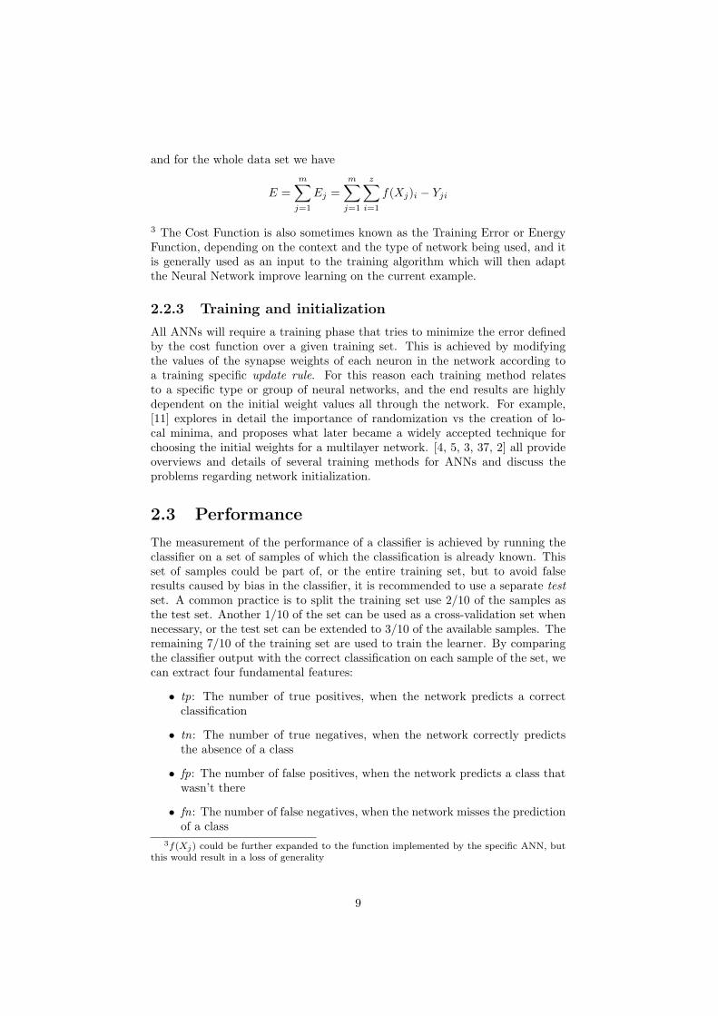
2.3 Performance

The measurement of the performance of a classifier is achieved by running theclassifier on a set of samples of which the classification is already known. Thisset of samples could be part of, or the entire training set, but to avoid falseresults caused by bias in the classifier, it is recommended to use a separate testset. A common practice is to split the training set use 2/10 of the samples asthe test set. Another 1/10 of the set can be used as a cross-validation set whennecessary, or the test set can be extended to 3/10 of the available samples. Theremaining 7/10 of the training set are used to train the learner. By comparingthe classifier output with the correct classification on each sample of the set, wecan extract four fundamental features:

• tp: The number of true positives, when the network predicts a correctclassification

• tn: The number of true negatives, when the network correctly predictsthe absence of a class

• fp: The number of false positives, when the network predicts a class thatwasn’t there

• fn: The number of false negatives, when the network misses the predictionof a class

3f(Xj) could be further expanded to the function implemented by the specific ANN, butthis would result in a loss of generality

9

2.3.1 Classification Error

Classification error is closely related to the training error, but is measured usinga separate and independent test seti T of size r, that shares no data with theoriginal training set, to prevent biased results (see ”Bias and Variance”). If weconsider, for each test set element j with Yj being the expected output vectorand θj the observed output vector, a measure of the error can be defined as 4 5:

∑r

j=1

∑n

i=1(Yji − θji)

2

r

This is an application of the Mean Squared Error (MSE) to the classificationprocess.

2.3.2 Misclassification

Another, very naive and immediate measure of performance for a classifier couldbe to just count how many classifications have been performed correctly out ofthe total number of samples, in the form Q

nwhere Q is the nnumber of samples

classified correctly.

2.3.3 Accuracy

Accuracy is the simplest of the possible measurements, and represents the abilityof a classifier to correctly make a prediction based on the current test set:

Accuracy =tp+ tn

tp+ tn+ fp+ fn

This measurement is subject to the bias of a one-sided sample distribution. Tobetter explain the problem, we can imagine a test set where 99% of the sampleshave a negative expectation and a classifier that always predicts no class (aconstant 0 output). The accuracy of this classifier would be:

Accuracy =0 + 0.99

1= 99%

which is clearly a bad (albeit a corner case) measurement of the real perfor-mance.

2.3.4 Precision and Recall

In order to avoid this issue, Precision and Recall have been devised. These twometrics are very efficient at measuring performance of classifiers even in the caseof a very one-sided sample distribution [31, 21, 47]. Precision can be thoughtof as the ratio of correct positive classification:

Precision =tp

tp+ fp

4the error is normalized to the test set size r to ensure that errors are comparable whentest sets have different sizes

5in this example outputs Yi are of the type R0..1; to make this measure comparable insigmoid-activated networks the result should be divided by 2

10

while Recall can be thought of as the ability of a classifier to find all the correctpositive classifications in the dataset:

Recall =tp

tp+ fn

2.3.5 F1-score

In order to understand correctly the performance of a classifier it is necessaryto use both precision and recall. A common mistake is to accept a classifierfor which only one of these two values is good. For this reason, rather thanusing two separate measures to be able to correctly measure the performanceof a classifier, these features can be used to work out the F1-score (sometimesalso called F-score or F-measure). This is the harmonic mean of precision andrecall:

F = 2 ·precision · recall

precision+ recall

2.3.6 Bias and Variance

Bias and variance are two measures of how well the classifier is fitted to theproblem. Adopting tr as the error on the training set and tt as the error on thetest set:

• A high variance occurs when a classifier performs very well on the trainingset compared to the test set, therefore implying overfitting : tt

tr>> 1, tt is

high, and tr is low.

• A high bias occurs when a classifier’s performance is lowly correlated toboth the training set and the test set. This means that both tr and tt arehigh. Paradoxically we can consider infinite bias in regards to a problemset to be equal to random performance.

[7] explores how training set size can affect bias and variance and reaches theinteresting conclusion that although variance seems to decrease with the increasein size of the training set, bias seems to remain unaffected. [19] explores indetail the effects of bias and variance in the specific case of neural networks,and concludes:

the bias/variance dilemma can be circumvented if one is willingto give up generality, that is, purposefully introduce bias. [. . . ] onemust ensure that the bias is in fact harmless for the problem at hand.

2.4 Weak learners

A weak learner is a learning algorithm with an error rate less than 50% - inother words a predictor that can do slightly better than making random guesses[24, 40]. Most of the time we will find that it easy to train a Neural Networkto become a weak classifier without incurring the risk of biasing it towardsthe training set. [40] formally introduces the equivalence of strong and weaklearnability, on top of which many of the concepts of ensemble learning arebuilt.

11

Chapter 3

Ensembles

In a general sense, Ensembles or Committees are a way of combining diverseweak classifiers into a single, stronger classifier. This can be achieved in manyways, and we can identify two important sub-problems: diversifying the weakclassifiers, and combining their outputs. For an in-depth review of classifierensembles, please refer to [48, 40].

3.1 History

The first idea to combine a number of classifiers was exposed in [9]. Thispaper does not go much beyond the idea of mixing a linear classifier with aNeural Network, albeit it introduces a very powerful concept of combinationand diversity. Undoubtedly, one of the pioneering documents on the subject is[40]. This piece of research introduces several new concepts and techniques:

• Weak learnability implies learnability. This means that no matter howweak a classifier, we can always construct a better one because the problemlends itself to be learned with arbitrarily low error.

• Combining multiple weak learners can lead to a stronger learner. Thismeans that we have a use for weak classifiers, and they can be a powerfultool.

• Hypothesis boosting algorithm. This shows a way we can achieve thestated goals.

Schapire then continues his work and cooperates with Freund on a new variantof boosting, publishing several papers and creating what is now known as theAdaBoost algorithm [41, 42, 44]. Meanwhile, Breiman produces [8] where he in-troduces the concept of ”bootstrap aggregating”, which will later become knownas bagging. Other significant works tackle the issue of combining the outputsof the weak classifiers, such as [25, 26, 16, 10], which introduce techniques likemajority voting, max min and median rules and several others. Since these ini-tal foundations have been laid, a large number of studies have been done, andI will cover more in the following sections, but the available literature is far toolarge to even be partially included in this document.

12

3.2 Overview

Because we can’t consider any given ANN, no matter how well it is trained,as a perfect classifier, intuition will suggest that the opinion of more that oneclassifier should lead to a better result. However, if said classifiers are identical,there is no change in the result. To obtain a better performing classifier we needto obtain diversity in the output set. This concept can be easily understoodby imagining a room full of people, who need to express an opinion about(classify) some data (an image, some text, a video, etc..). If there is onlyone person in the room, we are liable to all his mistakes. If there are manypeople we can imagine that if their opinions diverge, the collective will have ahigher probability of getting to the correct conclusion, and they will be able tocorrect the output of those who were wrong. If, however all the subjects alwaysreply unanimously, it would be the same as having only one person in theroom. A postulate to this intuition would be that, instead of only consideringweak classifiers (”all classifiers that do better than random”), we also considerbad classifiers (”classifiers that do worse than random”). These will then beconsidered with negative weight, therefore considering the inverse of their result.The important characteristic about ensembles is the the elements need to benegatively correlated, and they need to focus their error on different parts of thetraining set. This is generally achieved by introducing diversity. There are manytechniques that developed and they focus on either diversifying the training set,the topology of the network, or in some cases both. Many techniques on howthis diversity is recombined have also emerged over time, and the results varywidely. [48] contains a short proof of why a combination of weak learners willimprove on a single learner:

(it is) clear that we can reduce either the bias or the varianceto reduce the neural network error. Unfortunately, it is found thatfor the individual ANN concerned, the bias is reduced at the costof a large variance. However, the variance can be reduced by anensemble of ANNs, leaving the bias unchanged.

[5] covers ensembles (which he calls committees) in the last chapter and intro-duces the concept with an example:

[...] For instance, we might train L different models and thenmake predictions using the average of the predictions made by eachmodel. Such combinations of models are sometimes called com-mittes.

3.3 Training set diversity

We can diversify the training set in many ways:

3.3.1 Introduction of noise

The simplest way of creating many diverse training sets is to introduce randomtraining data generated using the distribution of the original training data as amodel. This allows to increase the size of the samples, from which to generatethe small training sets. It is shown that although this technique reduces bias,

13

it is not increasing variance[35]. A very good example of this technique is givenin the DECORATE (Diverse Ensemble Creation by Oppositional Relabeling ofArtificial Training Examples) study in [33], where the introduction of artificialtraining samples based on the training set’s distribution is shown to increasethe generalisation ability of ensembles with small training sets.

3.3.2 Bagging

In bagging the idea is to create n training sets by taking an original trainingset of size m and picking m elements from it, with resampling, n times. Thismeans that there will be overlap between the training sets (which keeps themcorrelated), but they will be diverse. This method can be made better if weensure during the resampling of each set, that it is not equal to a previouslyexisting set[8]. An example use of this methodology can be found in [34].

3.3.3 Boosting

The boosting technique also creates new training sets, but instead of randomlyresampling like with Bagging, we instead run each classifier as soon as its train-ing data is generated. We can then measure the performance of this classifierand use the results to retrain the next one to focus on the harder parts to learn.A well-known variant of boosting is adaptive boosting, or adaboost, where eachset of data is assigned a probability. Those data whose prediction is similar tothe training value receive an increasingly lower probability, and are thereforeless likely to be selected[40][41]. An example usage of Boosting can also befound in [34].

3.4 Architectural diversity

Another way of diversifying the components of an ensemble would be to usedifferent types of learners. This is not always guaranteed to provide negativecorrelation, but combined with differentiated training sets the likelyhood thateach component will focus its error on a different part of the set becomes higher.

3.4.1 Diverse Neural Groups

If we pick several different implementations of neural networks (provided thatwe keep the same output range), we can use them as separate members ofan ensemble. Diversity can be obtained by varying learning method, learningrate, network architecture (number of layers, number of neurons, etc), networktype (self-organizing, perceptrons, etc) and network-specific parameters. Anexample of this broadly defined technique was used in [12], where the authorsused evolutionary techniques to generate new emseble members. As long as theprinciple that these components perform differently than random and from eachother is maintained, the contribution of each should be non-zero 1 2. If each

1It is possible that the contribution may be negative or zero if the aggregation methodis not properly applied, but this requires adjustments in the aggregation rather than thediversification

2It is also possible that the contribution is so small to be approximable to zero. In such acase it would be better to discard the component and retry with different parameters in order

14

component network is visualized as an independent tree (although this may notbe strictly true), the ensemble effectively becomes a forest of neurons. This isa simple technique and its results may not be as good as the others presentedin this document. I plan to measure the performance and use it as a term ofcomparison to stacking.

3.5 Combining outputs

After managing to diversify all the different classifiers that make up the ensem-ble, the next step will be to combine these outputs in a way that will producea single classification based on the results of the ensemble components. Thereare several ways of doing this and each technique has its own benefits[25]. Wecan initially differentiate between two strategies of combining components:

• Consider only a part of all the members of the ensemble

• Use all the components

This means that in the first case we need to always select the best performingcandidates for each sample. It is helpful when classifiers have a ”degree ofcertainty” for their classification (for example how close their output is to 0 or13), especially if some classifiers perform well on a small subset of examples.

3.5.1 Averaging

Taking the average of the outputs is quick, and is very helpful when the compo-nents have different local minima (thus are ”diverse”) in reducing the ensemblevariance without increasing the bias by any significant amount[48]. A weightfactor w can be added to each component x such that

n∑

i=1

wi = 1

which will allow to give each vote a different impact on the final result

Y =n∑

i=1

wixi

It may be observed that this is the same function as the weighted sum of inputsin a neuron. This could be taken even further by applying the sigmoid functionP (t) defined in chapter 1, making this effectively another artificial neuron thatcould be trained. The constraint on the sum of the weights would no longerapply. This could be imagined as the simplest version possible of Stacking (seefurther).

to maximize the use of computational resources3We could formalise this by sorting in descending order for χ = (0.5− y)2

15

3.5.2 Majority voting

When using majority voting we consider the classification that was the outputof the highest number of classifiers. It is easy to see why it is called ”voting”and it is very straightforward to implement and understand, and executes veryquickly. A concrete discussion of the usage of the many majority voting variantsavailable is done in [17].

3.5.3 Stacking

In stacking we can take all the single weak classifiers we created using any ofthe previous techniques, and use them as input for a subsequent classifier. Thisrequires yet another split of the training set, such that a subset is left thathas not been used to train the first space classifiers. This new subset will beused to train the second space classifier[13]. This second dataset will have to bemodified to match the second space classifier’s inputs. We combine the outputsof all the first space classifiers based on the dataset’s input, and use them asinput values. The expected output remains unchanged.

3.5.4 Ranking

In order to implement ranking we need to make an essential modification to theunderlying classifiers, so that instead of providing a single classification optionthey will return a list of resulting classes ordered by relevance. There will bea selecting classifier that will look at the results of these ranked classificationsand choose the most suitable result [23][1]

16

Chapter 4

The Encog Library

Encog is an open source library maintained principally by Heaton Research,and it implements various techniques for machine learning and artificial in-telligence. It was initially developed in Java, but it has also been ported tomany other languages. For the scope of the project we will focus only on theJava implementation. The Java implementation of Encog is hosted on githubat https://github.com/encog/encog-java-core and is released under theApache license, which makes it very easy to work with and modify.

4.1 Architecture

Encog is structured as a single library, with many packages. Unfortunatelyat the time of writing no official UML diagrams were available for the Javaimplementation. Using UMLGraph to generate diagrams from the code revealsthat the complexity of the code is too high for the possibility of having a simplesignificant diagram to include in this documentation. I have however separatedsome portions of the library and tried to achieve an ”overall” view by describingseparate sections.

4.1.1 Machine Learning Packages

Encog includes the interfaces and classes for ML under org.encog.ml. For thepurpose of this document, I have included only the principal interfaces in thefollowing diagram.

17

https://github.com/encog/encog-java-core

BasicML

«interface»

MLAutoAssocation

«interface»

MLClassification

«interface»

MLCluster

«interface»

MLClustering

«interface»

MLContext

«interface»

MLEncodable

«interface»

MLError

«interface»

MLInput

«interface»

MLInputOutput

«interface»

MLMethod

«interface»

MLOutput

«interface»

MLProperties

«interface»

MLRegression

«interface»

MLResettable

«interface»

MLStateSequence

«interface»

Serializable

Figure 4.1: Basic encog ML package

These interfaces are used in most sections of Encog, either for the definitionof inputs and output (MLInput and MLOutput), to define a type of ML method(MLRegression and MLClassification) and other common properties that areeasily defined via inheritance, and that provide compatibility between similarobjects.

4.1.2 Neural Network Packages

In org.encog.neural we can find the neural network specific implementations.Most of these are implementations of ML interfaces, which is why I decided toimplement the ensemble techniques based on ML interfaces rather than Neuralinterfaces. The classes and interface that are most relevant to this project havebeen highlighted in light blue.

18

BAM

CPN AbstractPNN

BasicPNN RBFNetwork

SOM

ART ART1

NEATNetwork

BasicNetwork «interface»

ContainsFlat

BoltzmannMachine

HopfieldNetwork

ThermalNetwork

BasicML

BasicNeuralDataPair

BasicMLDataPair

BasicNeuralData

BasicMLData

«interface»

NeuralData «interface»

NeuralDataSet BasicMLDataSet

NeuralNetworkError

NeuralSimulatedAnnealingHelper

EncogError

NeuralDataMapping

PersistBasicNetwork

«interface»

NeuralDataPair BasicNeuralDataSet TrainingError PatternError

Figure 4.2: Common NN classes and interfaces in org.encog.neural

These classes provide the basic NN implementation. BasicNetwork providesa simple multi layer perceptron implementation that uses the NeuralData in-terface for input and output. NeuralDataSet provides an interface to definedatasets such as training sets or test sets. NeuralDataPair is an interface thatcontains one input datum and one output datum, making it suitable for super-vised learning. The Error family of classes provide an abstraction for represent-ing errors inside Encog.

19

NEATLink

NeuralStructure «interface»

Cloneable

NEATPopulation

NEATInnovation

NEATInnovationList

NEATNeuronGene

BasicLayer

TrainingContinuation

«interface»

Serializable

BasicGenome

BasicInnovation

BasicInnovationList

BasicGene

BasicPopulation

NEATGenome

NEATLinkGene

NeuralGenome

FlatNetworkRBF FlatLayer «interface»

Layer

FlatNetwork

NEATNeuron

PersistNEATNetwork

PersistNEATPopulation

PersistART1

PersistBAM

PersistCPN

NEATParams

AnalyzeNetwork

NetworkCODEC

NeuralPSOWorker PersistBasicPNN PersistHopfield

NeighborhoodBubble

«interface»

NeighborhoodFunction

NeighborhoodRBF

NeighborhoodRBF1D NeighborhoodSingle

RPROPConst SmartMomentum HiddenLayerParams PersistBoltzmann

ADALINEPattern

ART1Pattern BAMPattern

BoltzmannPattern CPNPattern ElmanPattern FeedForwardPattern HopfieldPattern

JordanPattern

«interface»

NeuralNetworkPattern

PNNPattern

RadialBasisPattern SOMPattern SVMPattern

NeuralGeneticAlgorithmHelper

BasicGeneticAlgorithm

NetworkFold

DeriveMinimum

Figure 4.3: NN architecture related classes and interfaces in org.encog.neural

Most of these classes implement features for more advanced NN algorithmsthat haven’t been used in this project, with the exception of the Layer family,which implement single layers inside a perceptron.

20

TrainInstar

TrainOutstar

NEATTraining

«interface»

CalculateScore

«interface»

LearningRate

«interface»

Momentum

«interface»

Train

TrainingSetScore

NeuralSimulatedAnnealing

ConcurrentTrainingManager

BPROPJob RPROPJob

TrainingJob

«interface»

ConcurrentTrainingPerformer

ConcurrentTrainingPerformerCPU

PerformerTask

CrossTraining

CrossValidationKFold

GeneticScoreAdapter

NeuralGeneticAlgorithm

LevenbergMarquardtTraining

«interface»

CalculationCriteria

GlobalMinimumSearch

TrainBasicPNN

GradientWorker

PersistTrainingContinuation

Propagation

Backpropagation

ManhattanPropagation

QuickPropagation

ResilientPropagation

ScaledConjugateGradient

NeuralPSO

TrainAdaline

SmartLearningRate

PruneIncremental

PersistRBFNetwork

SVD

SVDTraining

PersistSOM

BasicTrainSOM

BestMatchingUnit

SOMClusterCopyTraining

BasicTraining

GeneticAlgorithm

«interface»

Runnable

ConcurrentJob

ATanErrorFunction «interface»

ErrorFunction

LinearErrorFunction OutputErrorFunction

PruneSelective

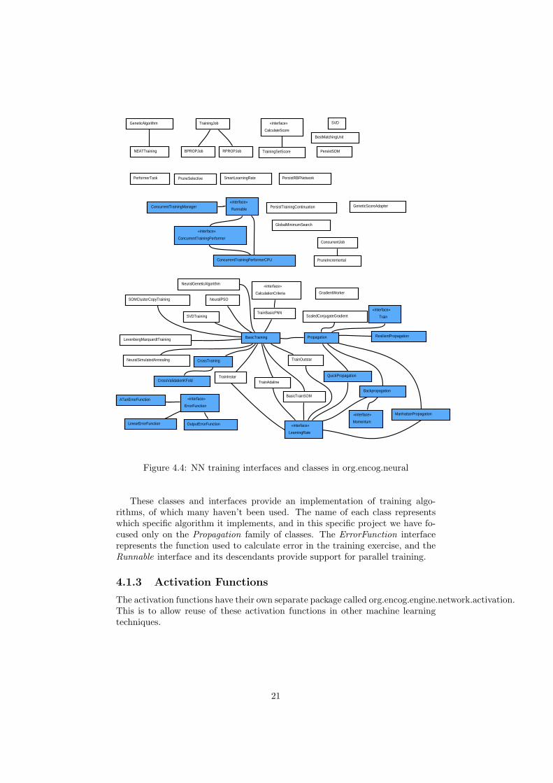
Figure 4.4: NN training interfaces and classes in org.encog.neural

These classes and interfaces provide an implementation of training algo-rithms, of which many haven’t been used. The name of each class representswhich specific algorithm it implements, and in this specific project we have fo-cused only on the Propagation family of classes. The ErrorFunction interfacerepresents the function used to calculate error in the training exercise, and theRunnable interface and its descendants provide support for parallel training.

4.1.3 Activation Functions

The activation functions have their own separate package called org.encog.engine.network.activation.This is to allow reuse of these activation functions in other machine learningtechniques.

21

ActivationBiPolar

ActivationBipolarSteepenedSigmoid

ActivationClippedLinear

ActivationCompetitive

ActivationElliott

ActivationElliottSymmetric

«interface»

ActivationFunction

ActivationGaussian ActivationLOG ActivationLinear ActivationRamp

ActivationSIN

ActivationSigmoid

ActivationSoftMax

ActivationSteepenedSigmoid

ActivationStep

ActivationTANH

«interface»

Serializable

«interface»

Cloneable

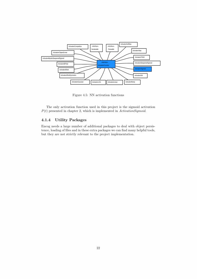
Figure 4.5: NN activation functions

The only activation function used in this project is the sigmoid activationP (t) presented in chapter 2, which is implemented in ActivationSigmoid.

4.1.4 Utility Packages

Encog needs a large number of additional packages to deal with object persis-tence, loading of files and in these extra packages we can find many helpful tools,but they are not strictly relevant to the project implementation.

22

Chapter 5

Implementation

5.1 Layout of the project

The code section of this project can be divided in two parts: one part relatesto the code changes to the Encog library itself, while the other relates to thesoftware written to obtain performance data. In terms of codebase size, it is aninteresting observation that more code was needed to implement the tests thanto implement the changes to Encog.

5.1.1 Packages

The following Java packages were created for benchmarking:

• ensembles

• helpers

• helpers.datasets

• perceptron

• techniques

and the following were added to Encog:

• org.encog.ensemble

• org.encog.ensemble.adaboost

• org.encog.ensemble.aggregator

• org.encog.ensemble.bagging

• org.encog.ensemble.data

• org.encog.ensemble.data.factories

• org.encog.ensemble.ml.mlp.factories

• org.encog.ensemble.training

23

5.2 Adding features to Encog

This section covers all the components that have added to Encog, at a medium-to-high level. For more implementation details, the reader is deferred to thejavadoc documentation generated or the source code itself.

5.2.1 Design decisions

One of the most interesting decisions was to change most interfaces to be ab-stract classes. This happened fairly late during the implementation, but reducedthe codebase considerably, and eliminated most of the repeated code. For thisreason interface can be used interchangeably with abstract class throughoutthis whole chapter. The decision to delegate responsibility to other interfaceswas also good, as it permitted easy implementation of new functionality in analmost completely pluggable fashion 1

5.2.2 Architectural changes

I have made a heavy use of Factory patterns and inheritance during the designprocess. This has allowed me to make the software structure very modular, andadding new implementations at a later date has revealed itself to be a simpletask from an architectural point of view. I tried to share as many interfaceswith the already existing parts of Encog as possible, although some had to beaggregated, as with EnsembleML.

5.2.3 Class design model

In this section the various components are presented and their functionalityexplained. They are separated by the interface they implement, which can beassociated with functionality groups.

Ensemble classes

This interface represents the main ensemble. It contains fields for all the otherinterfaces that are needed to implement complete ensemble functionality. Themethod of constructing a complete ensemble requires varied steps, dependingon the required characteristics. As a result of this, it lends itself well for be-ing used in a Builder pattern [18]. The generic model of this class type is touse an EnsembleDataSetFactory to create one new EnsembleDataSet for eachmember and to create the members themselves using an EnsembleMLMethod-Factory, which also requires a training method. Aggregation is done with anEnsembleAggregator and the training of the members is done using an Ensem-bleTrainFactory, both passed at instantiation time.

Bagging This class implements a version of Bagging. It uses the Resampling-DataSetFactory class to create the bootstrapped datasets which will then bepassed to whichever EnsembleMLMethodFactory is used to create the ensemblemembers.

1minor adjustments had to be made to the interfaces early on to permit some of the newalgorithms to fit in, but at a later stage it wasn’t necessary to modify the new interfaces anymore

24

AdaBoost This class implements the standard AdaBoost algorithm and usesa WeightedResamplingDataSetFactory to generate EnsembleDataSets that re-sample based on probability weights that are calculated at the training of eachmember. This method is particular because all the members have to be trainedsequentially.

Algorithm 1 Training in AdaBoost

procedure Train(ANN,TargetError) ⊲Initialize all members of D to 1/n ⊲ D is the weight vectorfor all i members do

Get a new training datasetCreate member i using the training factory and new datasetGet weighted error for new memberUpdate member weights vectorAdd member to main listUpdate D with new values

end for

end procedure

Stacking This is the implementation of Stacking, also known as Stacked Gen-eralization. Although the implementation allows for any EnsembleAggregatorto be used, it would not be a correct implementation if it didn’t use an instanceof Metaclassifier. Unfortunately there isn’t a way to impede the use of otherEnsembleAggregators without changing the Ensemble interface. This could beachieved with a language which easily supports type variants or runtime typemathing. Scala, Haskell and OCaml are all examples of such languages.

EnsembleAggregator classes

This family of classes implements the aggregation of the results via the evalu-ate function. This takes a list of computed outputs and performs the specificaggregation function, returning a new output of the same cardinality with thefinal decision.

Averaging This is a simple aggregator that returns the average of all theoutputs for each class.

MajorityVoting This is another simple aggregator that first thresholds theoutputs to put them in binary format, and then picks the output with thehighest vote count.

MetaClassifier This aggregator takes an EnsembleMLMethodFactory andan EnsembleTrainFactory at instantiation time, creates a classifier (the ”tier 2classifier” from Stacking), and trains it on a special training set that is generatedby aggregating the outputs of all classifiers for each instance of the originaltraining set. The final output is then the output of this classifier when presentedwith the ensemble member outputs.

25

EnsembleDataSetFactory

These classes generate data sets for training ensemble members, by implement-ing the getNewDataSet function, which returns a new dataset of size k, specifiedat initialization. An initialization dataset will have to be given, from which thedata instances are picked.

ResamplingDataSetFactory This factory will generate datasets of size k,by randomly picking entries from the initalization data set, with resampling.

WeightedResamplingDataSetFactory This factory will return data by ran-domly picking entries from the initialization data set, with resampling, and bytaking account of a weight vector U .

WrappingNonResamplingDataSetFactory This factory will always re-turn the k entries between k∗i and k∗(i+1), with i being the count of times thatgetNewDataSet has been called before. If the end of the initialization datasetis reached, then the search wraps back to the beginning ad infinitum.

EnsembleML classes

The EnsembleML interface adds functionality on top of the MLMethod class inEncog, and implements the function of an ensemble member. The reason forhaving this interface is to allow new sub-types of this class to be implementedtransparently to the current code, to allow new techniques to be implemented.

GenericEnsembleML This is the generic implementation of an EnsembleML.No other implementations were necessary at this stage, but it did not seem ap-propriate to remove the generality provided by having the separate interface.

EnsembleMLMethodFactory classes

These factories generate ensemble members of type EnsembleML, and requirean EnsembleTrainFactory and an EnsembleDataSetFactory to operate.

MultiLayerPerceptronFactory This factory create multi-layer perceptronsby taking a specification of activation function and layers, under the form of alist of integers.

EnsembleTrainFactory

This family of factories will create the training methods (of type MLTrain) thatwill be used in EnsembleML.

BackpropagationFactory This class implements regular backpropagation[3]

LevenbergMarquardtFactory This class implements LMA [29]

26

ManhattanPropagationFactory This class implements Manhattan propa-gation [36]

ResilientPropagationFactory This class implements Resilient propagation[36]

ScaledConjugateGradientFactory This class implements the Scaled Con-jugate Gradient algorithm [32]

EnsembleTypes

Ensemble

<<MLMethod,MlClassification,MLRegression>>

EnsembleML

EnsembleMLMethodFactory

EnsembleTrainFactory

<<Ensemble>>

AdaBoost

<<EnsembleML>>

GenericEnsembleML

EnsembleAggregator

<<EnsembleAggregator>>

MajorityVoting<<EnsembleAggregator>>

Averaging

<<Ensemble>>

Bagging

<<MLDataSet>>

EnsembleDataSetEnsembleDataSetFactory

<<EnsembleDataSetFactory>>

ResamplingDataSetFactory


WeightedResamplingDataSetFactory

<<EnsembleMLMethodFactory>>

MultiLayerPerceptronFactory

<<EnsembleTrainFactory>>

ResilientPropagationFactory


BackpropagationFactory


ScaledConjugateGradientFactory

<<EnsembleAggregator>>

MetaClassifier

<<Ensemble>>

Stacking


WrappingNonResamplingDataSetFactory


ManhattanPropagationFactory


LevenbergMarquardtPropagationFactory

Figure 5.1: Class diagram of added components

5.3 Creating a framework for testing

A challenge has certainly been the benchmarking of the new techniques. Theimplementation has required the creation of a framework, albeit very small, fordescribing and loading datasets, applying an ensemble learner, and extractingresults. This is without considering all the necessary tools to actually run thebenchmarks.

5.4 Source management

In order to manage such a complex codebase, it was necessary to adopt somemeasure to store revisions, source distribution between hosts (also for backups),and automate building and testing.

5.4.1 Revision control

The source code for Encog is hosted on github (https://github.com/encog), sothe straightforward solution to managing all the Java code for this project was

27

to use git. This should simplify the patch submission process. All other filesrelated to the project (including the project proposal and this report) are storedin a separate mercurial repository. The main reason for choosing mercurial isits simpler merging mechanism and approach to multiple heads. A convenientside-effect of this choice is that it is impossible to accidentally attempt to mergethe project-related repository with the encog repository.

5.4.2 Automated building

In order to use up-to-date code in the simulations, some sort of automatedcompilation and building of the sources was required. I opted for an ant buildscript because it had the lowest requirements and was the easiest method toimplement quickly. This was enough to make sure that building the sources forthe jobs did not require a full recompilation at every job submission.

28

Chapter 6

Benchmarking the newfeatures

6.1 Running tests

In order to obtain data to show the efficacy of the various ensemble approaches,it has been necessary to run the test program on a variety of datasets and collectthe data on performance in respect to the ensemble size, collect the data, andrepresent it in a graphical way that highlights the immediate validity of thetechniques under test.

6.1.1 The test plan

For each dataset, the plan is to find some semi-optimal single-perceptron param-eters, and try to improve on the performance of that perceptron by applying,in turn, all the ensemble techniques, with all the member output aggregationmethods, in a linear search for the optimal number of ensemble components(this has been limited between 1 and 300, mostly due to time limitation). Thisgenerates a series of results that can be graphed in respect to the ensemble size.

6.1.2 The test program

The test program is a relatively simple piece of code that will read a predefinedproblem description file, take input parameters on how to create and train anensemble to learn the dataset, and evaluate the performance of the ensemble onboth the training data and a dynamically determined test set.

Arguments

All the command line arguments to the testing tool are in one way or anotherrelated to the definition of which technique and which parameters to use tocreate and train the ensemble. In order, they are:

• technique: the ensemble technique to use for this run (bagging, adaboost)

• problem: the problem set description file

29

• sizes: comma separated list of ensemble sizes to try

• dataSetSizes: comma separated list of sizes for generated ensemble train-ing sets

• trainingErrors: comma separated list of target training errors

• trainingSetSize: size of the original training set (used to generate theensemble training sets)

• activationThreshold: the minimum value for an output to be considered 1

• training: training algorithm (rprop, backprop, scg)

• membertypes: description of the ensemble members architecture in theform method:parameters:activation (e.g. mlp:100:sigmoid)

• aggregator: the method used to aggregate the outputs of each ensemblecomponent (majorityvoting, averaging)

• verbose: whether to print out all intermediate training values (useful forplotting ”training curves”)

Dataset description

In order to make it easy to load in different datasets, I have made the datasetdescription an external configuration file. This contains all the values needed toparse the dataset files correctly and to perform one-vs-all classification in thecorrect manner on the specified dataset. The descriptor file contains entries inthe ¡setting¿=¡value¿ format:

• label: what label to use in the output, to identify this dataset.

• outpus: how many output classes there are

• inputs: how many input classes there are

• read inputs: how many columns contain the classification values for thetraining data

• inputs reversed: if true, the input classification is before the input values

• mapper type: what mapping to use for the classification representation

• data file: the path of the CSV containing the training set data

Output

The output is in CSV format on stdout at execution time, and contains thefollowing fields, in order:

• the label of the problem set

• what set this is (test/training)

• the ensemble technique used in this run

30

• the training method used

• the type of ensemble members

• the layout of the ensemble members

• the aggregator used to decide the output

• the size of the ensemble

• the size of the data set

• the target training error

• the misclassification

• microaveraged accuracy

• microaveraged precision

• microaveraged recall

• microaveraged F1

• macroaveraged accuracy

• macroaceraged precision

• macroaveraged recall

• macroaveraged F1

6.2 Infrastructure layout

6.2.1 The PBS system

In order to efficiently run several test jobs with so many different parameters,it has revealed itself convenient to use a batch system. The system of choice isTORQUE (http://www.adaptivecomputing.com/products/open-source/torque).It is one of the many derivatives of the original OpenPBS and is reasonablystraightforward to setup and manage. In order to preserve security when run-ning a PBS system distributed across several physical locations, I have optedfor routing all PBS traffic over an Openvpn network. It has revealed itself nec-essary to write a few patches for TORQUE, which have been submitted backto the community for review.

6.2.2 AWS compute nodes

The large number of simulations, and the necessity to be able to re-run sometests towards the end of the project, have made it necessary to create a systemthat was flexible in terms of size. Amazon Web Services has served well as anenabler of elastic instances that could run these jobs ”out of the box”. A nodeimage has been devised, such that at first boot it would configure itself to joina virtual private network, connect to the master PBS node, and start executingjobs instantly. At peak times there have been 25 compute nodes, and the easewith which it was possible to turn them on and off at will has undoubtedlysimplified the execution part of the project by a great deal.

31

6.2.3 Submission tools

To make submission to the PBS system possible I had to write a set of scriptsthat would manage output handling, ensure that the test application was up todate at run time, and speed up creation of new job scripts. run job contains allthe basic functions, but the real job wrapper scripts are named by the job typethey represent. All submissions are made in the form of job arrays 1, and thejob index is used as the ensemble size for that specific benchmark run.

Environment

Scripts like run-environment.sh are responsible for updating the source tree fromgit, compiling all the framework using ant, and creating aliases and shortcutsto make job definition more standardised. These scripts and the ant build.xmldefinition file live with the framework source code in encog-checkout/src/runs.

Job Scripts

The job scripts are responsible for calling out to the environment, setting upinput data where necessary, and submitting the output data to the mercurialrepository. Examples of these are in the batch jobs directory.

6.2.4 Aggregating results

All results are committed into the projects/mscproject/runs output subdirectoryof the mercurial repository. generate csv.sh creates a csv with all the results,which facilitates importing into a worksheet program like oocalc or Excel.

6.2.5 Creating graphs and tables

In order to create all the graphs and tables contained in this report, a tool ofmodest complexity was needed, so that the process could be automated and re-run at several stages of the project. make graphs and tables.pl is a Perl scriptthat takes all the necessary steps to create the material, and deposits it in thecorrect place for it to be included in the report compilation, done by build.sh.

6.3 The data sets

All the real-life datasets used for testing are taken from the UCI machine learn-ing repository (http://archive.ics.uci.edu/ml/). I have also used a tool calleddatasetgenerator (http://code.google.com/p/datasetgenerator/) to generate ex-act datasets, to verify the algorithms. All datasets have been split in trainingand test sets (as per the discussion in 2.3), and the performance has been mea-sured for both sets in all cases, so to facilitate the spotting of overfitting. Themeasure of performance that seems more appropriate when looking at the outputin this case seems to be misclassification, as defined in 2.3, as it represents the”number of mistakes”, which can be easily understood. The size of each trainingset and test set has been predefined, but the selection of which instances make

1In a PBS system, a job array is a shortcut for submitting multiple copies of the same job,and each one receives an index number at execution through the environment.

32

it into the training set is a random process that happens in runtime, and hastherefore different results every time. The remaining instances are used in thetest set. The reason for doing this is to avoid giving an unexpected advantageto any specific technique. These are all the dataset (generated and non) thathave been used:

6.3.1 Haberman’s Survival

This is the data resulting from a study on the survival rate of patients afterreceiving surgical treatment for breast cancer

• URL: http://archive.ics.uci.edu/ml/datasets/Haberman’s+Survival

• Relevant papers: [22, 27, 30]

• Data instances: 306

• Training set size: 200

• Inputs: 3

• Output classes: 2, in numeric format (1 field)

6.3.2 Letter Recognition

This dataset contains a number of statistical and edge properties of some char-acters and the purpose of the classification is to establish which letter of thealphabet is represented in the rectangular section of pixels described by theseproperties.

• URL: http://archive.ics.uci.edu/ml/datasets/Letter+Recognition

• Relevant papers: [15]



• Inputs: 16

• Output classes: 26, in letter format (1 field)

6.3.3 Landsat

In this dataset there is a small section of a scan from the NASA Landsat satellite,with each line representing a 3x3 pixel area, with readings in 4 spectral bands.The goal is to classify the type of soil contained in the pixel area. This datasethas been discussed by many authors, including Schapire and Freund themselveswhile discussing Boosting algorithms.

• URL: http://archive.ics.uci.edu/ml/datasets/Letter+Recognition

• Relevant papers: [43, 45, 20, 46] and many more, referenced on the dataset’sweb page.

33



• Inputs: 36


6.3.4 Magic

This dataset contains generated data that simulates high energy gamma particleobservations in an atmospheric Cherenkov telescope. I have chosen this datasetbeacuse it has a large number of instances and given that it is a generateddataset it should be easier to find a working machine learning technique tomodel the set.

• URL: http://archive.ics.uci.edu/ml/datasets/MAGIC+Gamma+Telescope

• Relevant papers: [14, 39, 6]



• Inputs: 11


6.4 Reducing the search space

Because of the large number of options available for tweaking, the search spacefor optimal settings for the test runs is very large. A few ”tricks” have beennecessary in order to reduce both the dimensionality of this space and the boundsof each dimension searched.

6.4.1 Previous literature

In order to improve the effectiveness of the search for optimal parameters, I havetried to extract ideas from previous literature on the specific datasets (whereapplicable). This helped pick good starting points. All literature that appliesto a specific dataset is mentioned in that dataset’s specific section.

6.4.2 Picking parameters

In order to reduce the search space even further, I have extracted empiricallygood parameters for the single classifier example, for each of the problems. Thisinvolved plotting ”learning curves” for each neural architecture, which plot theMSE in relation to the training iteration, as well as the training and test setmisclassification, at each step of the training process. The most convenient wayis to use the existing framework, with bagging-1 and averaging. This should beequivalent to running a NN classifier on its own.

34

Ensemble Member Type

The main goal of creating these ”learning curves” is to be able to pick anensemble component type for each problem without having to run benchmarksacross the whole space of possible member types. We already know by thelimitation set out before commencing the exercise that the only members willbe multi layer perceptrons (although they may not be optimal learners for theseproblems). The space of how many neurons, the training method, the trainingtarget error still need to be searched.

Training Method The space searched for training methods contains mostlypropagation-type trainers, and includes Resilient Propagation, Back Propa-gation, Manhattan Update Rule, Scaled Conjugate Gradient and Levenberg-Marquardt. It turns out that for these problems, using only simple multi-layerperceptrons, the best option is to use Resilient Propagation in all cases. It isreasonably quick and provides decent results.

Target Training Error All propagation training in Encog requires a ”target”internal mean-squared error (MSE) to which the ANN is trained. The basicalgorithm is as follows:

Algorithm 2 Encog basic propagation algorithm

procedure Train(ANN,TargetError) ⊲ Train an ANN to this TargetErrorwhile getError(ANN) ¿ TargetError do

PerformTrainingIteration(ANN)end while

end procedure

35

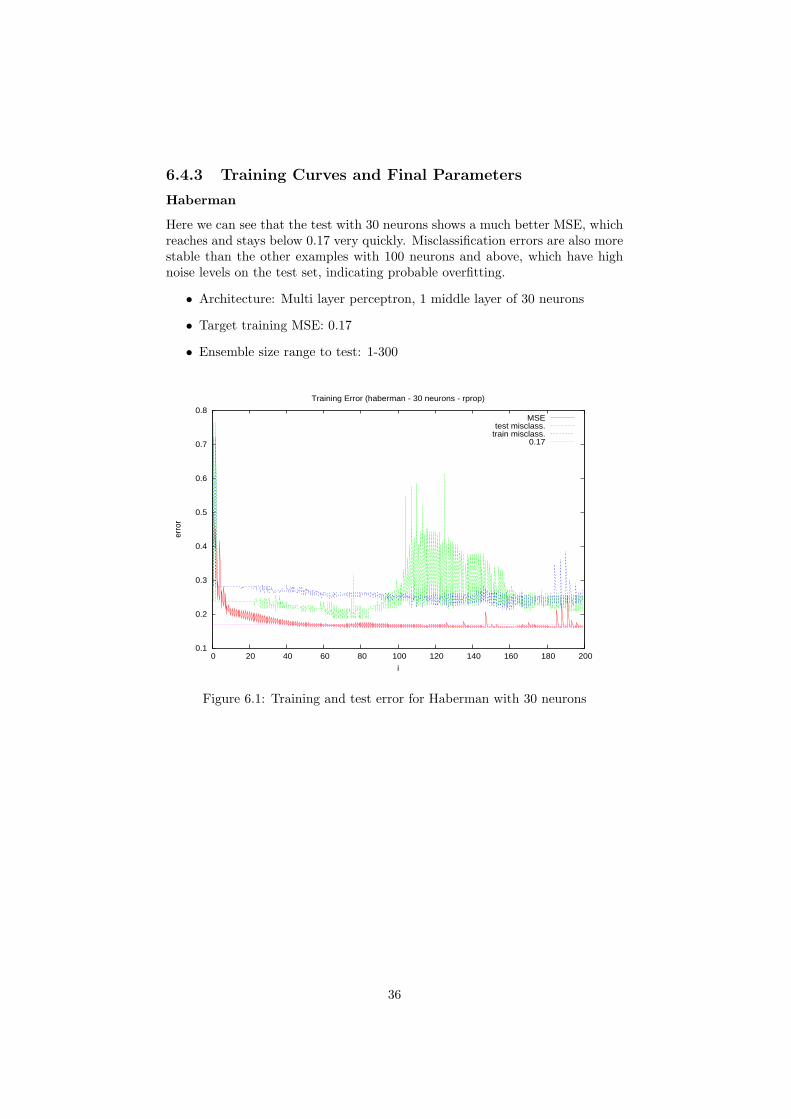
6.4.3 Training Curves and Final Parameters

Haberman

Here we can see that the test with 30 neurons shows a much better MSE, whichreaches and stays below 0.17 very quickly. Misclassification errors are also morestable than the other examples with 100 neurons and above, which have highnoise levels on the test set, indicating probable overfitting.

• Architecture: Multi layer perceptron, 1 middle layer of 30 neurons

• Target training MSE: 0.17

• Ensemble size range to test: 1-300

0.1

0.2

0.3

0.4

0.5

0.6

0.7

0.8

0 20 40 60 80 100 120 140 160 180 200

erro

r

i

Training Error (haberman - 30 neurons - rprop)

MSEtest misclass.

train misclass.0.17

Figure 6.1: Training and test error for Haberman with 30 neurons

36

0.1

0.2

0.3

0.4

0.5

0.6

0.7

0.8

0.9

1

0 20 40 60 80 100 120 140 160 180 200

erro

r

i


MSEtest misclass.

train misclass.0.17


0.1

0.2

0.3

0.4

0.5

0.6

0.7

0.8

0.9

1

0 20 40 60 80 100 120 140 160 180 200

erro

r

i


MSEtest misclass.

train misclass.0.17


37

Letter Recognition

This problem set seems to have an MSE that descends quickly below 0.05 andthen moves very slowly after the first few training iterations. Noise levels arevery low for the first 500 iterations for both 100 and 300 neurons, while anythingbelow 100 does not seem to have enough capacity to learn all the patterns. Weseem to be gaining more correct result as the training continues, although thenoise levels that appear at around the 650th iteration may indicate that that isthe point where we start overfitting the data.




0

0.1

0.2

0.3

0.4

0.5

0.6

0.7

0.8

0.9

1

0 100 200 300 400 500 600 700 800 900 1000

erro

r

i

Training Error (letterrecognition - 30 neurons - rprop)

MSEtest misclass.

train misclass.0.015

Figure 6.4: Training and test error for Letter Recognition with 30 neurons

38

0

0.1

0.2

0.3

0.4

0.5

0.6

0.7

0.8

0.9

1

0 100 200 300 400 500 600 700 800 900 1000

erro

r

i


MSEtest misclass.



0

0.1

0.2

0.3

0.4

0.5

0.6

0.7

0.8

0.9

1

0 100 200 300 400 500 600 700 800 900 1000

erro

r

i


MSEtest misclass.



39

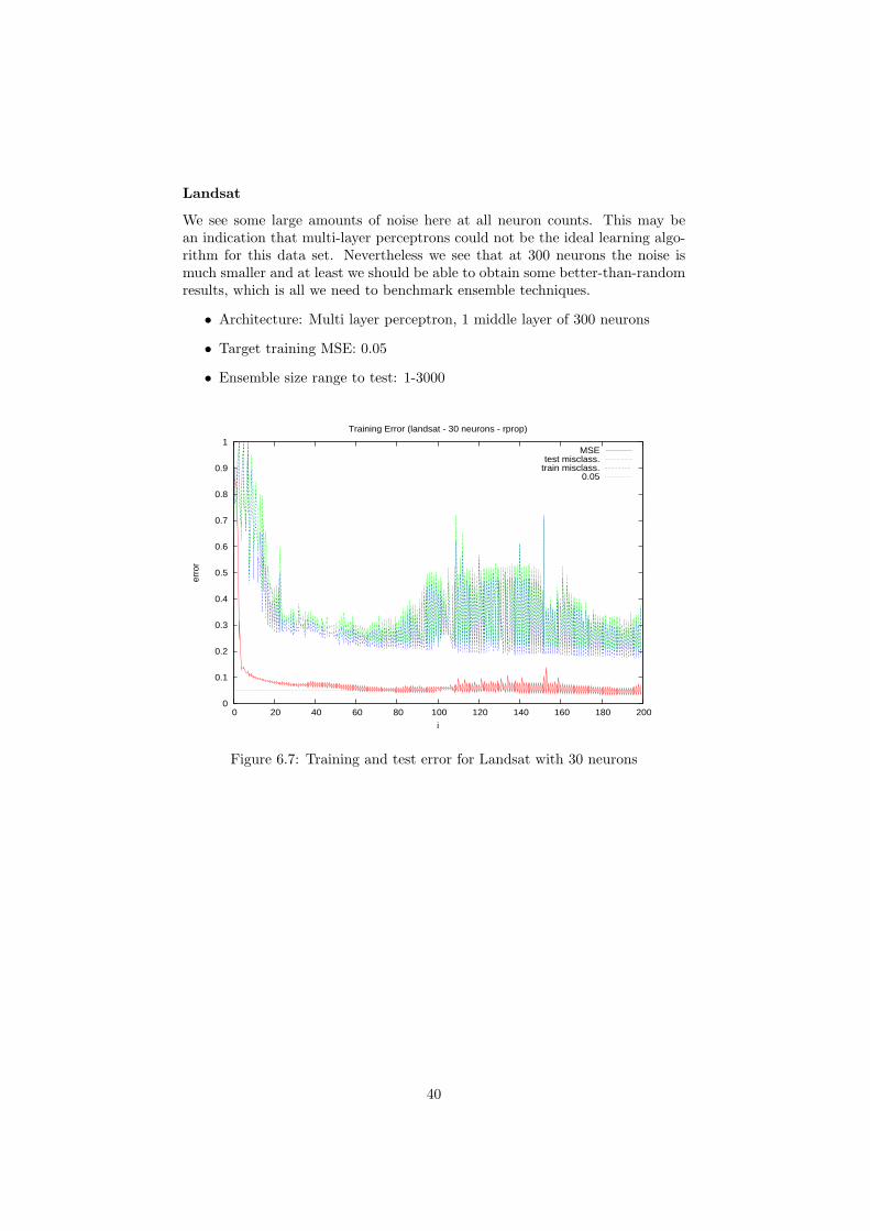
Landsat

We see some large amounts of noise here at all neuron counts. This may bean indication that multi-layer perceptrons could not be the ideal learning algo-rithm for this data set. Nevertheless we see that at 300 neurons the noise ismuch smaller and at least we should be able to obtain some better-than-randomresults, which is all we need to benchmark ensemble techniques.




0

0.1

0.2

0.3

0.4

0.5

0.6

0.7

0.8

0.9

1

0 20 40 60 80 100 120 140 160 180 200

erro

r

i

Training Error (landsat - 30 neurons - rprop)

MSEtest misclass.

train misclass.0.05

Figure 6.7: Training and test error for Landsat with 30 neurons

40

0

0.1

0.2

0.3

0.4

0.5

0.6

0.7

0.8

0.9

1

0 20 40 60 80 100 120 140 160 180 200

erro

r

i


MSEtest misclass.

train misclass.0.05


0

0.1

0.2

0.3

0.4

0.5

0.6

0.7

0.8

0.9

1

0 20 40 60 80 100 120 140 160 180 200

erro

r

i


MSEtest misclass.

train misclass.0.05


41

Magic

The MAGIC Telescope dataset appears to be a hard set to generalize for a multi-layer perceptron. The performance at 100 and 300 neurons is almost identical,and the noise level is very low. With these parameters being very similar, theassumption is that the cheapest of the two options is better.




0

0.2

0.4

0.6

0.8

1

0 20 40 60 80 100 120 140 160 180 200

erro

r

i

Training Error (magic - 30 neurons - rprop)

MSEtest misclass.

train misclass.0.10

Figure 6.10: Training and test error for Magic with 30 neurons

42

0

0.2

0.4

0.6

0.8

1

0 20 40 60 80 100 120 140 160 180 200

erro

r

i


MSEtest misclass.

train misclass.0.10


43

0

0.2

0.4

0.6

0.8

1

0 20 40 60 80 100 120 140 160 180 200

erro

r

i


MSEtest misclass.

train misclass.0.10


44

6.4.4 Dividing ranges

In order to improve the time required to run these searches, I have found it usefulto divide each parameter’s space into smaller ranges, so that several separatejobs could be run at once. This made the search quicker without having toreduce the search space itself, at the cost of utilizing more hardware.

45

Chapter 7

Test results

In this chapter the raw results collected from the benchmarks are presented.For each possible combination of ensemeble technique, voting mechanism andproblem set the following data have been generated:

1. a commentary of the data obtained from the benchmark

2. a table illustrating the average of the performance values for both the testand training datasets for each ensemble size 1

3. a graph illustrating the performance measures for the test set, in relationto the ensemble size

4. a graph illustrating the performance measures for the training set, in re-lation to the ensemble size

5. a per-class accuracy histogram for each ensemble size

6. further considerations, if any

For succintness, only the data information worthy of commentary has beenincluded in this chapter, while all the other generated graphs can be found inthe data plots/final directory of the project repository.

Each benchmark has been run a minimum of 3 times, to ensure that thedata is less fallible to outliers. Characteristic traits that we look out for in thedata are:

• Measurement improvements. For all the measure we are looking for indi-cation that increasing the ensemble size produces better results. Ideallythis is represented by local minima (or maximums) in the measurements.

• Optimal ensemble sizes (or ranges). We are looking for ranges on the xaxis where the performance measurements adopt lower values. Ideally thelocal minima from the previous characteristic lie in this region.

• Noise reduction. We are looking for ranges where the variance in theperformance measurements is reduced.

1The term ”ensemble size” refers to the number of members of the ensemble used for aspecific benchmark

46

• Class bias. It is possible that a classifier may be performing better forcertain classes, so we extract a histogram of accuracy on each class for thetraining set. If there is a class that is clearly outperforming or underper-forming we may have class bias. This is an especially well-known problemwith multilayer perceptrons, and there are training techniques to remedythis [28].

7.1 Bagging


Haberman

It would seem that in this case we get a stable, good performance at around7 ensemble members. After this the measurements do not decline heavily, butthe variance in the results does not seem to decrease much so there is notmuch to gain in adding the extra computational complexity. The per-classperformance seems to be also stable, although there seems to be an imbalancetowards selecting class 0. This may be just a side effect of the prior probabilitydifference P (1) << P (0), given that the number of samples for class 0 is muchlarger in this dataset.

47

Table 7.1: Performance for the haberman dataset (bagging - majorityvoting)size test/train runs misc σ2 ma acc σ2 ma prec ma rec ma F1

1 test 4 0.241 0.059 0.763 0.583 0.529 0.557 0.538

1 train 4 0.269 0.073 0.732 0.536 0.516 0.578 0.541

2 test 3 0.352 0.149 0.737 0.546 0.685 0.498 0.566

2 train 3 0.312 0.098 0.734 0.539 0.657 0.514 0.577

3 test 2 0.241 0.058 0.776 0.602 0.705 0.580 0.635

3 train 2 0.282 0.080 0.731 0.535 0.669 0.583 0.622

4 test 4 0.257 0.066 0.762 0.580 0.657 0.579 0.615

4 train 4 0.286 0.082 0.749 0.561 0.714 0.565 0.631

5 test 2 0.236 0.056 0.764 0.584 0.645 0.572 0.606

5 train 2 0.250 0.063 0.752 0.567 0.733 0.590 0.652

6 test 3 0.236 0.056 0.781 0.611 0.700 0.574 0.630

6 train 3 0.288 0.083 0.741 0.549 0.718 0.527 0.607

7 test 4 0.233 0.055 0.772 0.597 0.610 0.578 0.589

7 train 4 0.269 0.073 0.739 0.546 0.610 0.570 0.584

8 test 1 0.208 0.043 0.792 0.628 0.723 0.615 0.665

8 train 1 0.270 0.073 0.740 0.548 0.678 0.601 0.637

9 test 3 0.236 0.056 0.763 0.582 0.643 0.592 0.616

9 train 3 0.253 0.064 0.750 0.563 0.689 0.591 0.636

10 test 2 0.241 0.058 0.764 0.584 0.646 0.559 0.599

10 train 2 0.280 0.079 0.748 0.559 0.723 0.556 0.626

15 test 1 0.226 0.051 0.769 0.591 0.636 0.520 0.572

15 train 1 0.280 0.078 0.720 0.518 0.612 0.511 0.557

20 test 2 0.241 0.058 0.764 0.584 0.627 0.573 0.598

20 train 2 0.255 0.065 0.751 0.565 0.744 0.577 0.649

30 test 1 0.226 0.051 0.778 0.606 0.706 0.581 0.638

30 train 1 0.280 0.078 0.728 0.529 0.655 0.551 0.598

60 test 1 0.236 0.056 0.769 0.591 0.676 0.561 0.613

60 train 1 0.270 0.073 0.728 0.529 0.620 0.540 0.577

100 test 1 0.226 0.051 0.778 0.606 0.706 0.581 0.638

100 train 1 0.275 0.076 0.722 0.522 0.596 0.531 0.561

0.2

0.3

0.4

0.5

0.6

0.7

0.8

0 10 20 30 40 50 60 70 80 90 100

err

or

ensemble size

test error measurements (haberman-bagging-majorityvoting)

Misclassificationm.a. accuracym.a. precision

m.a. recall

0

0.1

0.2

0.3

0.4

0.5

0.6

0.7

0 10 20 30 40 50 60 70 80 90 100

var(

x)

ensemble size

test error variance (haberman-bagging-majorityvoting)


m.a. recall

Figure 7.1: Performance on the Haberman dataset (test set) for Bagging withMajority Voting

48

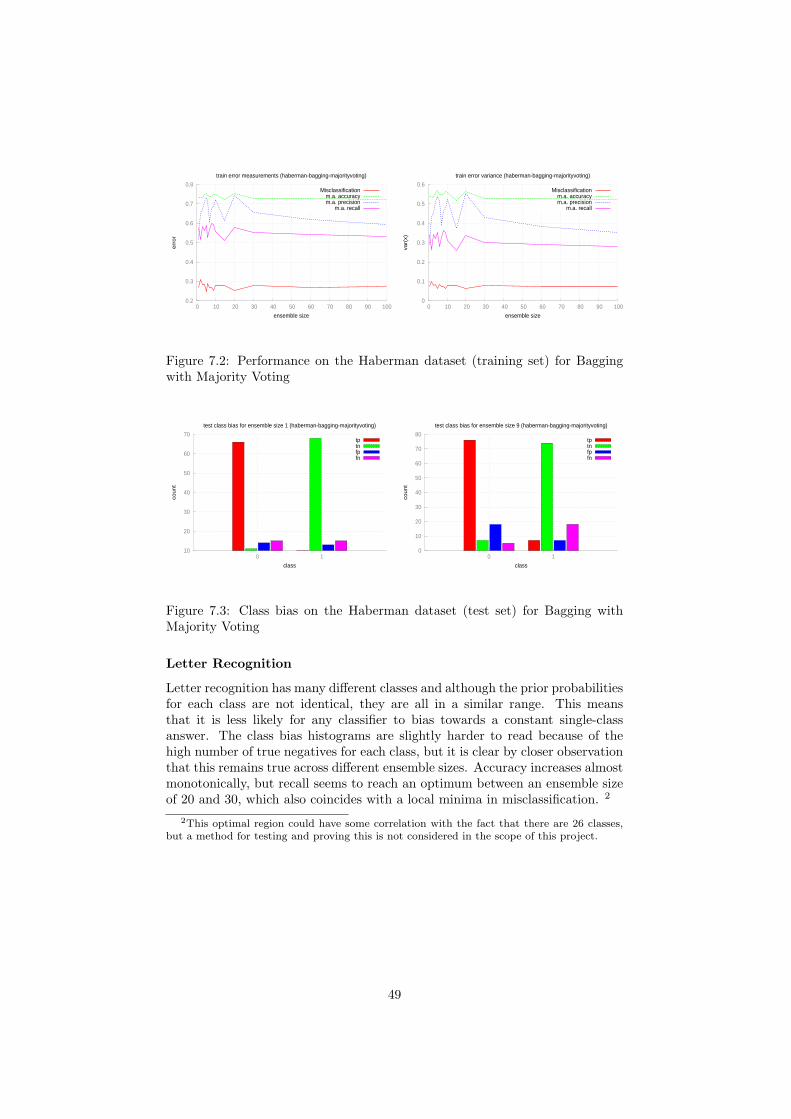
0.2

0.3

0.4

0.5

0.6

0.7

0.8

0 10 20 30 40 50 60 70 80 90 100

err

or

ensemble size

train error measurements (haberman-bagging-majorityvoting)


m.a. recall

0

0.1

0.2

0.3

0.4

0.5

0.6

0 10 20 30 40 50 60 70 80 90 100

var(

x)

ensemble size

train error variance (haberman-bagging-majorityvoting)


m.a. recall

Figure 7.2: Performance on the Haberman dataset (training set) for Baggingwith Majority Voting

10

20

30

40

50

60

70

0 1

count

class

test class bias for ensemble size 1 (haberman-bagging-majorityvoting)

tptnfpfn

0

10

20

30

40

50

60

70

80

0 1

count

class

test class bias for ensemble size 9 (haberman-bagging-majorityvoting)

tptnfpfn

Figure 7.3: Class bias on the Haberman dataset (test set) for Bagging withMajority Voting

Letter Recognition

Letter recognition has many different classes and although the prior probabilitiesfor each class are not identical, they are all in a similar range. This meansthat it is less likely for any classifier to bias towards a constant single-classanswer. The class bias histograms are slightly harder to read because of thehigh number of true negatives for each class, but it is clear by closer observationthat this remains true across different ensemble sizes. Accuracy increases almostmonotonically, but recall seems to reach an optimum between an ensemble sizeof 20 and 30, which also coincides with a local minima in misclassification. 2

2This optimal region could have some correlation with the fact that there are 26 classes,but a method for testing and proving this is not considered in the scope of this project.

49

Table 7.2: Performance for the letterrecognition dataset (bagging - majorityvot-ing)size test/train runs misc σ2 ma acc σ2 ma prec ma rec ma F1

1 test 3 0.488 0.243 0.979 0.958 0.830 0.530 0.646

1 train 3 0.468 0.225 0.980 0.960 0.857 0.547 0.666

2 test 3 0.532 0.289 0.979 0.958 0.913 0.473 0.621

2 train 3 0.512 0.269 0.979 0.959 0.916 0.490 0.636

3 test 2 0.511 0.267 0.979 0.958 0.878 0.504 0.637

3 train 2 0.490 0.246 0.980 0.960 0.902 0.522 0.658

4 test 3 0.504 0.261 0.980 0.960 0.911 0.505 0.646

4 train 3 0.484 0.241 0.980 0.961 0.923 0.520 0.662

5 test 2 0.502 0.258 0.979 0.959 0.883 0.510 0.644

5 train 2 0.482 0.239 0.980 0.961 0.923 0.528 0.668

6 test 2 0.517 0.274 0.979 0.959 0.871 0.493 0.628

6 train 2 0.497 0.254 0.980 0.960 0.911 0.507 0.648

7 test 3 0.472 0.228 0.981 0.961 0.901 0.541 0.674

7 train 3 0.454 0.212 0.981 0.963 0.923 0.555 0.690

8 test 3 0.484 0.242 0.980 0.961 0.906 0.526 0.663

8 train 3 0.465 0.224 0.981 0.963 0.908 0.540 0.675

9 test 2 0.501 0.257 0.980 0.959 0.916 0.511 0.652

9 train 2 0.479 0.236 0.980 0.961 0.926 0.529 0.670

10 test 2 0.522 0.279 0.979 0.958 0.900 0.488 0.629

10 train 2 0.499 0.256 0.980 0.960 0.914 0.506 0.648

15 test 1 0.592 0.350 0.976 0.953 0.912 0.416 0.571

15 train 1 0.570 0.325 0.977 0.955 0.930 0.434 0.592

20 test 2 0.506 0.263 0.979 0.959 0.895 0.504 0.642

20 train 2 0.487 0.244 0.980 0.961 0.919 0.518 0.659

30 test 2 0.507 0.265 0.979 0.959 0.901 0.503 0.642

30 train 2 0.486 0.243 0.980 0.961 0.939 0.519 0.664

60 test 1 0.591 0.350 0.976 0.953 0.920 0.416 0.573

60 train 1 0.568 0.323 0.977 0.955 0.939 0.435 0.595

100 test 1 0.587 0.345 0.977 0.954 0.868 0.420 0.566

100 train 1 0.566 0.320 0.977 0.955 0.937 0.437 0.596

0.4

0.5

0.6

0.7

0.8

0.9

1

0 10 20 30 40 50 60 70 80 90 100

err

or

ensemble size

test error measurements (letterrecognition-bagging-majorityvoting)


m.a. recall

0.1

0.2

0.3

0.4

0.5

0.6

0.7

0.8

0.9

1

0 10 20 30 40 50 60 70 80 90 100

var(

x)

ensemble size

test error variance (letterrecognition-bagging-majorityvoting)


m.a. recall

Figure 7.4: Performance on the Letter Recognition dataset (test set) for Baggingwith Majority Voting

50

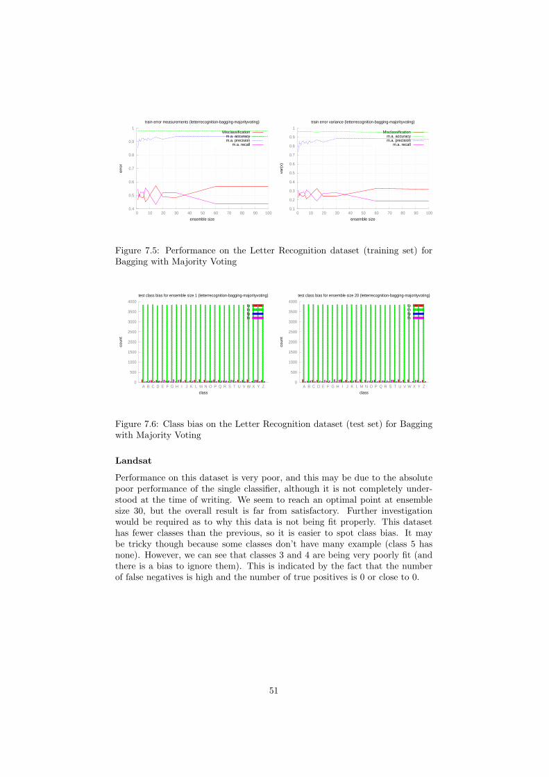
0.4

0.5

0.6

0.7

0.8

0.9

1

0 10 20 30 40 50 60 70 80 90 100

err

or

ensemble size

train error measurements (letterrecognition-bagging-majorityvoting)


m.a. recall

0.1

0.2

0.3

0.4

0.5

0.6

0.7

0.8

0.9

1

0 10 20 30 40 50 60 70 80 90 100

var(

x)

ensemble size

train error variance (letterrecognition-bagging-majorityvoting)


m.a. recall

Figure 7.5: Performance on the Letter Recognition dataset (training set) forBagging with Majority Voting

0

500

1000

1500

2000

2500

3000

3500

4000

A B C D E F G H I J K L M N O P Q R S T U V W X Y Z

count

class

test class bias for ensemble size 1 (letterrecognition-bagging-majorityvoting)

tptnfpfn

0

500

1000

1500

2000

2500

3000

3500

4000


count

class

test class bias for ensemble size 20 (letterrecognition-bagging-majorityvoting)

tptnfpfn

Figure 7.6: Class bias on the Letter Recognition dataset (test set) for Baggingwith Majority Voting

Landsat

Performance on this dataset is very poor, and this may be due to the absolutepoor performance of the single classifier, although it is not completely under-stood at the time of writing. We seem to reach an optimal point at ensemblesize 30, but the overall result is far from satisfactory. Further investigationwould be required as to why this data is not being fit properly. This datasethas fewer classes than the previous, so it is easier to spot class bias. It maybe tricky though because some classes don’t have many example (class 5 hasnone). However, we can see that classes 3 and 4 are being very poorly fit (andthere is a bias to ignore them). This is indicated by the fact that the numberof false negatives is high and the number of true positives is 0 or close to 0.

51

Table 7.3: Performance for the landsat dataset (bagging - majorityvoting)size test/train runs misc σ2 ma acc σ2 ma prec ma rec ma F1

1 test 4 0.447 0.223 0.928 0.861 0.588 0.431 0.496

1 train 4 0.407 0.199 0.933 0.872 0.607 0.450 0.514

2 test 4 0.434 0.201 0.932 0.868 0.599 0.439 0.507

2 train 4 0.394 0.172 0.937 0.878 0.603 0.462 0.523

3 test 3 0.420 0.184 0.932 0.869 0.612 0.449 0.518

3 train 3 0.376 0.150 0.938 0.881 0.622 0.470 0.535

4 test 4 0.466 0.239 0.928 0.862 0.637 0.425 0.507

4 train 4 0.409 0.186 0.935 0.875 0.612 0.452 0.519

5 test 3 0.459 0.220 0.928 0.861 0.571 0.428 0.489

5 train 3 0.403 0.172 0.935 0.875 0.577 0.454 0.507

6 test 4 0.438 0.209 0.931 0.867 0.630 0.442 0.517

6 train 4 0.384 0.166 0.938 0.880 0.633 0.470 0.537

7 test 3 0.439 0.206 0.929 0.863 0.610 0.442 0.512

7 train 3 0.377 0.153 0.938 0.879 0.593 0.470 0.524

8 test 4 0.425 0.191 0.932 0.868 0.589 0.451 0.511

8 train 4 0.369 0.144 0.939 0.882 0.599 0.476 0.530

9 test 3 0.421 0.185 0.933 0.870 0.615 0.452 0.521

9 train 3 0.363 0.139 0.940 0.884 0.619 0.479 0.540

10 test 4 0.452 0.227 0.928 0.862 0.592 0.439 0.504

10 train 4 0.386 0.165 0.937 0.878 0.636 0.466 0.535

15 test 1 0.521 0.272 0.922 0.849 0.532 0.381 0.444

15 train 1 0.465 0.217 0.929 0.863 0.538 0.397 0.457

20 test 2 0.513 0.289 0.921 0.848 0.583 0.398 0.471

20 train 2 0.441 0.214 0.930 0.866 0.562 0.424 0.483

30 test 3 0.438 0.203 0.931 0.866 0.615 0.445 0.516

30 train 3 0.376 0.151 0.939 0.881 0.622 0.470 0.535

60 test 3 0.435 0.200 0.931 0.867 0.616 0.446 0.516

60 train 3 0.377 0.152 0.938 0.881 0.618 0.471 0.534

100 test 3 0.440 0.208 0.930 0.865 0.615 0.443 0.514

100 train 3 0.378 0.154 0.938 0.880 0.618 0.470 0.533

0.3

0.4

0.5

0.6

0.7

0.8

0.9

1

0 10 20 30 40 50 60 70 80 90 100

err

or

ensemble size

test error measurements (landsat-bagging-majorityvoting)


m.a. recall

0.1

0.2

0.3

0.4

0.5

0.6

0.7

0.8

0.9

0 10 20 30 40 50 60 70 80 90 100

var(

x)

ensemble size

test error variance (landsat-bagging-majorityvoting)


m.a. recall

Figure 7.7: Performance on the Landsat dataset (test set) for Bagging withMajority Voting

52

0.3

0.4

0.5

0.6

0.7

0.8

0.9

1

0 10 20 30 40 50 60 70 80 90 100

err

or

ensemble size

train error measurements (landsat-bagging-majorityvoting)


m.a. recall

0.1

0.2

0.3

0.4

0.5

0.6

0.7

0.8

0.9

0 10 20 30 40 50 60 70 80 90 100

var(

x)

ensemble size

train error variance (landsat-bagging-majorityvoting)


m.a. recall

Figure 7.8: Performance on the Landsat dataset (training set) for Bagging withMajority Voting

0

200

400

600

800

1000

1200

1400

1600

0 1 2 3 4 5 6

count

class

test class bias for ensemble size 1 (landsat-bagging-majorityvoting)

tptnfpfn

0

200

400

600

800

1000

1200

1400

1600

0 1 2 3 4 5 6

count

class

test class bias for ensemble size 20 (landsat-bagging-majorityvoting)

tptnfpfn

Figure 7.9: Class bias on the Landsat dataset (test set) for Bagging with Ma-jority Voting

Magic

A very disappointing run can be found in this combination of dataset and tech-nique. On the test set, all ensemble sizes, there is a clear bias towards class 1shown in the histograms. This is much better on the training sets, and whenthe observation is combined with the actual performance measures, it is clearlyan indication that this technique is overfitting the training set, and is thereforebiased. Something that could help fix this problem could be to change the tar-get training error to a higher value. This was not tried because of a lack of timewhen this observation was made at the end of the project.

53

Table 7.4: Performance for the magic dataset (bagging - majorityvoting)size test/train runs misc σ2 ma acc σ2 ma prec ma rec ma F1

1 test 3 0.506 0.266 0.509 0.267 0.500 0.258 0.339

1 train 3 0.142 0.020 0.860 0.740 0.838 0.737 0.784

2 test 3 0.512 0.263 0.524 0.275 0.500 0.244 0.328

2 train 3 0.156 0.025 0.859 0.739 0.850 0.717 0.778

3 test 3 0.503 0.254 0.506 0.256 0.500 0.252 0.335

3 train 3 0.141 0.020 0.861 0.741 0.845 0.733 0.785

4 test 2 0.513 0.264 0.504 0.255 0.500 0.245 0.328

4 train 2 0.149 0.022 0.858 0.735 0.842 0.721 0.777

5 test 3 0.489 0.241 0.519 0.271 0.500 0.260 0.342

5 train 3 0.139 0.019 0.863 0.744 0.843 0.741 0.788

6 test 2 0.513 0.265 0.503 0.255 0.500 0.244 0.327

6 train 2 0.148 0.022 0.858 0.736 0.843 0.723 0.778

7 test 3 0.498 0.249 0.508 0.260 0.500 0.254 0.336

7 train 3 0.140 0.020 0.862 0.743 0.848 0.734 0.787

8 test 2 0.502 0.253 0.505 0.256 0.500 0.250 0.333

8 train 2 0.146 0.021 0.857 0.734 0.837 0.726 0.778

9 test 3 0.483 0.234 0.523 0.274 0.500 0.262 0.344

9 train 3 0.138 0.019 0.863 0.745 0.845 0.741 0.790

10 test 2 0.518 0.270 0.490 0.241 0.500 0.243 0.327

10 train 2 0.144 0.021 0.858 0.736 0.842 0.724 0.779

15 test 1 0.551 0.303 0.456 0.208 0.500 0.228 0.313

15 train 1 0.158 0.025 0.845 0.713 0.822 0.702 0.757

20 test 2 0.500 0.252 0.505 0.256 0.500 0.250 0.333

20 train 2 0.143 0.021 0.859 0.738 0.842 0.728 0.781

30 test 3 0.490 0.240 0.513 0.264 0.500 0.256 0.339

30 train 3 0.139 0.020 0.862 0.743 0.847 0.736 0.788

60 test 1 0.528 0.279 0.474 0.225 0.500 0.237 0.322

60 train 1 0.156 0.024 0.844 0.713 0.814 0.708 0.757

100 test 2 0.500 0.251 0.503 0.254 0.500 0.251 0.334

100 train 2 0.142 0.020 0.859 0.737 0.840 0.730 0.781

0.2

0.25

0.3

0.35

0.4

0.45

0.5

0.55

0.6

0 10 20 30 40 50 60 70 80 90 100

err

or

ensemble size

test error measurements (magic-bagging-majorityvoting)


m.a. recall

0.05

0.1

0.15

0.2

0.25

0.3

0.35

0 10 20 30 40 50 60 70 80 90 100

var(

x)

ensemble size

test error variance (magic-bagging-majorityvoting)


m.a. recall

Figure 7.10: Performance on the Magic dataset (test set) for Bagging withMajority Voting

54

0.1

0.2

0.3

0.4

0.5

0.6

0.7

0.8

0.9

0 10 20 30 40 50 60 70 80 90 100

err

or

ensemble size

train error measurements (magic-bagging-majorityvoting)


m.a. recall

0

0.1

0.2

0.3

0.4

0.5

0.6

0.7

0.8

0 10 20 30 40 50 60 70 80 90 100

var(

x)

ensemble size

train error variance (magic-bagging-majorityvoting)


m.a. recall

Figure 7.11: Performance on the Magic dataset (training set) for Bagging withMajority Voting

0

200

400

600

800

1000

1200

1400

1600

1800

0 1

count

class

test class bias for ensemble size 1 (magic-bagging-majorityvoting)

tptnfpfn

0

200

400

600

800

1000

1200

1400

1600

1800

0 1

count

class

test class bias for ensemble size 10 (magic-bagging-majorityvoting)

tptnfpfn

Figure 7.12: Class bias on the Magic dataset (test set) for Bagging with MajorityVoting

0

2000

4000

6000

8000

10000

12000

0 1

count

class

train class bias for ensemble size 1 (magic-bagging-majorityvoting)

tptnfpfn

0

2000

4000

6000

8000

10000

12000

14000

0 1

count

class

train class bias for ensemble size 10 (magic-bagging-majorityvoting)

tptnfpfn

Figure 7.13: Class bias on the Magic dataset (training set) for Bagging withMajority Voting

7.1.2 Averaging

Given the similarity between the two approaches, there are not many differencesto be expected in the results.

55

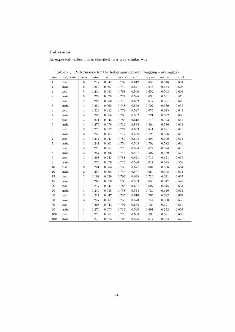
Haberman

As expected, haberman is classified in a very similar way.

Table 7.5: Performance for the haberman dataset (bagging - averaging)size test/train runs misc σ2 ma acc σ2 ma prec ma rec ma F1

1 test 6 0.217 0.047 0.782 0.612 0.655 0.616 0.631

1 train 6 0.259 0.067 0.740 0.547 0.648 0.574 0.603

2 test 5 0.230 0.053 0.768 0.590 0.652 0.563 0.604

2 train 5 0.279 0.078 0.724 0.525 0.630 0.531 0.573

3 test 4 0.224 0.050 0.776 0.602 0.677 0.587 0.629

3 train 4 0.254 0.065 0.748 0.559 0.707 0.580 0.636

4 test 4 0.229 0.052 0.772 0.597 0.675 0.615 0.644

4 train 4 0.235 0.055 0.763 0.582 0.721 0.622 0.668

5 test 3 0.211 0.045 0.786 0.618 0.713 0.593 0.647

5 train 3 0.275 0.076 0.732 0.535 0.804 0.530 0.634

6 test 3 0.226 0.052 0.777 0.603 0.641 0.581 0.610

6 train 3 0.252 0.064 0.747 0.558 0.728 0.576 0.642

7 test 3 0.217 0.047 0.780 0.608 0.699 0.609 0.651

7 train 3 0.247 0.061 0.750 0.563 0.702 0.582 0.636

8 test 3 0.226 0.051 0.770 0.594 0.674 0.574 0.618

8 train 3 0.257 0.066 0.746 0.557 0.597 0.569 0.576

9 test 1 0.208 0.043 0.788 0.621 0.716 0.621 0.665

9 train 1 0.275 0.076 0.725 0.526 0.617 0.525 0.568

10 test 2 0.231 0.053 0.759 0.577 0.604 0.566 0.584

10 train 2 0.255 0.065 0.746 0.557 0.669 0.568 0.614

15 test 1 0.198 0.039 0.792 0.628 0.720 0.621 0.667

15 train 1 0.265 0.070 0.730 0.533 0.658 0.547 0.597

20 test 1 0.217 0.047 0.788 0.621 0.697 0.615 0.654

20 train 1 0.240 0.058 0.758 0.574 0.724 0.610 0.662

30 test 3 0.217 0.047 0.785 0.616 0.705 0.622 0.661

30 train 3 0.247 0.061 0.755 0.570 0.744 0.590 0.658

60 test 1 0.208 0.043 0.797 0.635 0.724 0.621 0.669

60 train 1 0.270 0.073 0.735 0.540 0.691 0.542 0.607

100 test 1 0.226 0.051 0.778 0.606 0.706 0.581 0.638

100 train 1 0.270 0.073 0.725 0.526 0.617 0.534 0.573

56

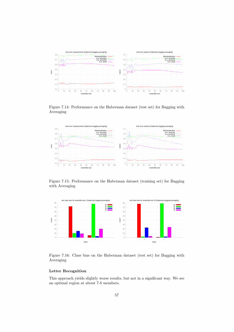
0.1

0.2

0.3

0.4

0.5

0.6

0.7

0.8

0 10 20 30 40 50 60 70 80 90 100

err

or

ensemble size

test error measurements (haberman-bagging-averaging)


m.a. recall

0

0.1

0.2

0.3

0.4

0.5

0.6

0.7

0 10 20 30 40 50 60 70 80 90 100

var(

x)

ensemble size

test error variance (haberman-bagging-averaging)


m.a. recall

Figure 7.14: Performance on the Haberman dataset (test set) for Bagging withAveraging

0.2

0.3

0.4

0.5

0.6

0.7

0.8

0.9

0 10 20 30 40 50 60 70 80 90 100

err

or

ensemble size

train error measurements (haberman-bagging-averaging)


m.a. recall

0

0.1

0.2

0.3

0.4

0.5

0.6

0.7

0 10 20 30 40 50 60 70 80 90 100

var(

x)

ensemble size

train error variance (haberman-bagging-averaging)


m.a. recall

Figure 7.15: Performance on the Haberman dataset (training set) for Baggingwith Averaging

0

10

20

30

40

50

60

70

80

0 1

count

class

test class bias for ensemble size 1 (haberman-bagging-averaging)

tptnfpfn

0

10

20

30

40

50

60

70

80

0 1

count

class

test class bias for ensemble size 10 (haberman-bagging-averaging)

tptnfpfn

Figure 7.16: Class bias on the Haberman dataset (test set) for Bagging withAveraging

Letter Recognition

This approach yields slightly worse results, but not in a significant way. We seean optimal region at about 7-8 members.

57

Table 7.6: Performance for the letterrecognition dataset (bagging - averaging)size test/train runs misc σ2 ma acc σ2 ma prec ma rec ma F1

1 test 3 0.367 0.138 0.979 0.958 0.836 0.539 0.653

1 train 3 0.344 0.121 0.980 0.960 0.854 0.555 0.670

2 test 3 0.396 0.160 0.977 0.955 0.848 0.481 0.612

2 train 3 0.378 0.146 0.978 0.957 0.853 0.494 0.624

3 test 2 0.375 0.144 0.979 0.959 0.892 0.508 0.644

3 train 2 0.354 0.129 0.980 0.961 0.912 0.525 0.663

4 test 2 0.363 0.136 0.979 0.959 0.909 0.500 0.641

4 train 2 0.345 0.123 0.980 0.960 0.922 0.514 0.655

5 test 1 0.429 0.184 0.976 0.953 0.914 0.409 0.565

5 train 1 0.411 0.169 0.977 0.954 0.935 0.423 0.582

6 test 2 0.365 0.137 0.979 0.959 0.895 0.501 0.639

6 train 2 0.346 0.124 0.980 0.961 0.932 0.520 0.663

7 test 3 0.340 0.118 0.981 0.962 0.929 0.540 0.680

7 train 3 0.321 0.105 0.982 0.964 0.931 0.554 0.691

8 test 2 0.361 0.134 0.979 0.959 0.887 0.501 0.638

8 train 2 0.343 0.122 0.980 0.961 0.931 0.519 0.662

9 test 2 0.361 0.134 0.980 0.959 0.903 0.507 0.646

9 train 2 0.342 0.120 0.981 0.961 0.929 0.526 0.668

10 test 2 0.365 0.137 0.980 0.960 0.915 0.509 0.651

10 train 2 0.345 0.123 0.981 0.962 0.936 0.529 0.672

15 test 1 0.426 0.182 0.977 0.954 0.858 0.418 0.562

15 train 1 0.406 0.165 0.977 0.955 0.861 0.434 0.577

20 test 2 0.362 0.134 0.980 0.960 0.928 0.509 0.654

20 train 2 0.341 0.120 0.981 0.962 0.936 0.524 0.668

30 test 1 0.422 0.178 0.977 0.954 0.897 0.421 0.573

30 train 1 0.405 0.164 0.977 0.955 0.936 0.437 0.596

60 test 1 0.419 0.175 0.977 0.954 0.863 0.421 0.566

60 train 1 0.402 0.162 0.978 0.956 0.941 0.438 0.598

0.3

0.4

0.5

0.6

0.7

0.8

0.9

1

0 10 20 30 40 50 60

err

or

ensemble size

test error measurements (letterrecognition-bagging-averaging)


m.a. recall

0.1

0.2

0.3

0.4

0.5

0.6

0.7

0.8

0.9

1

0 10 20 30 40 50 60

var(

x)

ensemble size

test error variance (letterrecognition-bagging-averaging)


m.a. recall

Figure 7.17: Performance on the Letter Recognition dataset (test set) for Bag-ging with Averaging

58

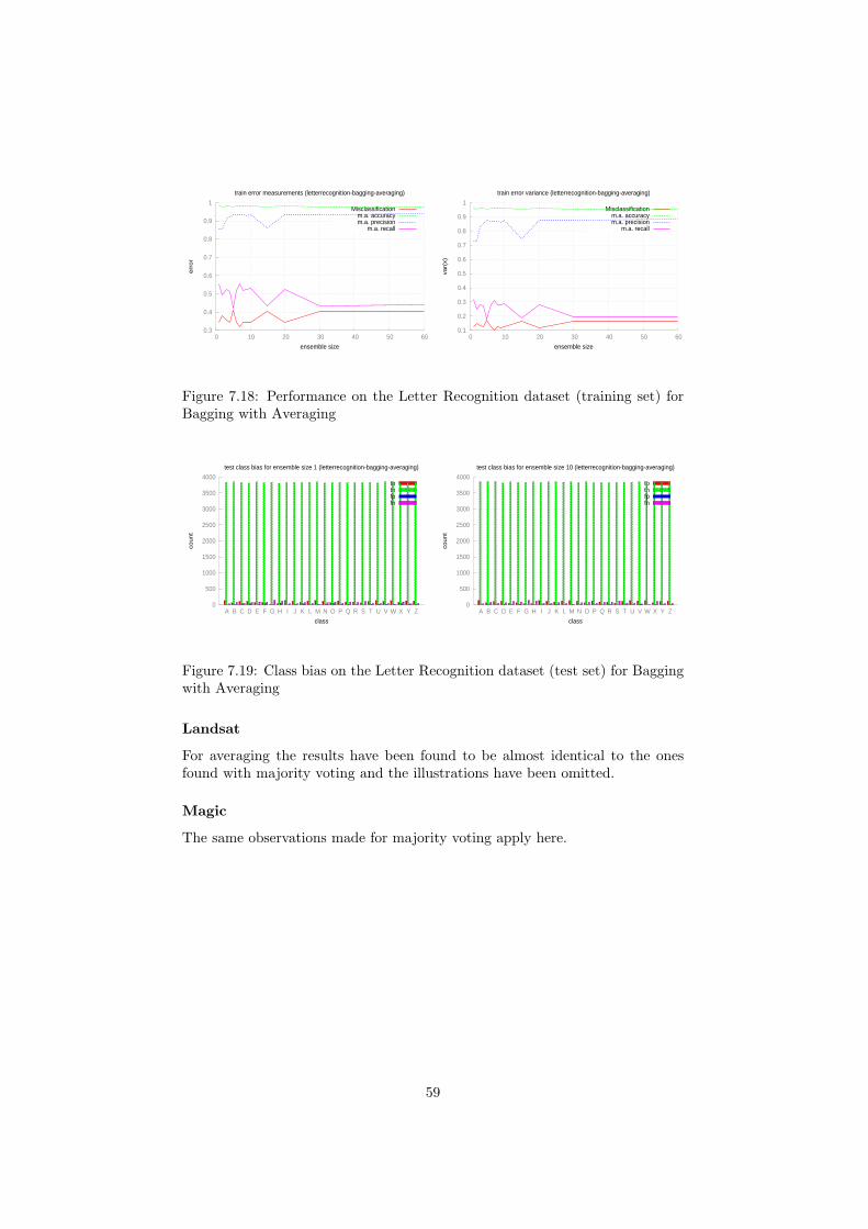
0.3

0.4

0.5

0.6

0.7

0.8

0.9

1

0 10 20 30 40 50 60

err

or

ensemble size

train error measurements (letterrecognition-bagging-averaging)


m.a. recall

0.1

0.2

0.3

0.4

0.5

0.6

0.7

0.8

0.9

1

0 10 20 30 40 50 60

var(

x)

ensemble size

train error variance (letterrecognition-bagging-averaging)


m.a. recall

Figure 7.18: Performance on the Letter Recognition dataset (training set) forBagging with Averaging

0

500

1000

1500

2000

2500

3000

3500

4000


count

class

test class bias for ensemble size 1 (letterrecognition-bagging-averaging)

tptnfpfn

0

500

1000

1500

2000

2500

3000

3500

4000


count

class

test class bias for ensemble size 10 (letterrecognition-bagging-averaging)

tptnfpfn

Figure 7.19: Class bias on the Letter Recognition dataset (test set) for Baggingwith Averaging

Landsat

For averaging the results have been found to be almost identical to the onesfound with majority voting and the illustrations have been omitted.

Magic

The same observations made for majority voting apply here.

59

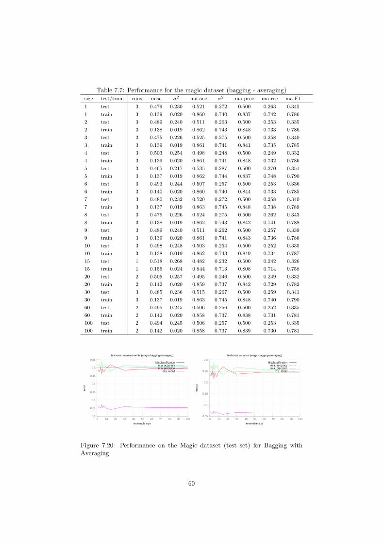
Table 7.7: Performance for the magic dataset (bagging - averaging)size test/train runs misc σ2 ma acc σ2 ma prec ma rec ma F1

1 test 3 0.479 0.230 0.521 0.272 0.500 0.263 0.345

1 train 3 0.139 0.020 0.860 0.740 0.837 0.742 0.786

2 test 3 0.489 0.240 0.511 0.263 0.500 0.253 0.335

2 train 3 0.138 0.019 0.862 0.743 0.848 0.733 0.786

3 test 3 0.475 0.226 0.525 0.275 0.500 0.258 0.340

3 train 3 0.139 0.019 0.861 0.741 0.841 0.735 0.785

4 test 3 0.503 0.254 0.498 0.248 0.500 0.249 0.332

4 train 3 0.139 0.020 0.861 0.741 0.848 0.732 0.786

5 test 3 0.465 0.217 0.535 0.287 0.500 0.270 0.351

5 train 3 0.137 0.019 0.862 0.744 0.837 0.748 0.790

6 test 3 0.493 0.244 0.507 0.257 0.500 0.253 0.336

6 train 3 0.140 0.020 0.860 0.740 0.844 0.733 0.785

7 test 3 0.480 0.232 0.520 0.272 0.500 0.258 0.340

7 train 3 0.137 0.019 0.863 0.745 0.848 0.738 0.789

8 test 3 0.475 0.226 0.524 0.275 0.500 0.262 0.343

8 train 3 0.138 0.019 0.862 0.743 0.842 0.741 0.788

9 test 3 0.489 0.240 0.511 0.262 0.500 0.257 0.339

9 train 3 0.139 0.020 0.861 0.741 0.843 0.736 0.786

10 test 3 0.498 0.248 0.503 0.254 0.500 0.252 0.335

10 train 3 0.138 0.019 0.862 0.743 0.849 0.734 0.787

15 test 1 0.518 0.268 0.482 0.232 0.500 0.242 0.326

15 train 1 0.156 0.024 0.844 0.713 0.808 0.714 0.758

20 test 2 0.505 0.257 0.495 0.246 0.500 0.249 0.332

20 train 2 0.142 0.020 0.859 0.737 0.842 0.729 0.782

30 test 3 0.485 0.236 0.515 0.267 0.500 0.259 0.341

30 train 3 0.137 0.019 0.863 0.745 0.848 0.740 0.790

60 test 2 0.495 0.245 0.506 0.256 0.500 0.252 0.335

60 train 2 0.142 0.020 0.858 0.737 0.838 0.731 0.781

100 test 2 0.494 0.245 0.506 0.257 0.500 0.253 0.335

100 train 2 0.142 0.020 0.858 0.737 0.839 0.730 0.781

0.2

0.25

0.3

0.35

0.4

0.45

0.5

0.55

0 10 20 30 40 50 60 70 80 90 100

err

or

ensemble size

test error measurements (magic-bagging-averaging)


m.a. recall

0.05

0.1

0.15

0.2

0.25

0.3

0 10 20 30 40 50 60 70 80 90 100

var(

x)

ensemble size

test error variance (magic-bagging-averaging)


m.a. recall

Figure 7.20: Performance on the Magic dataset (test set) for Bagging withAveraging

60

0.1

0.2

0.3

0.4

0.5

0.6

0.7

0.8

0.9

0 10 20 30 40 50 60 70 80 90 100

err

or

ensemble size

train error measurements (magic-bagging-averaging)


m.a. recall

0

0.1

0.2

0.3

0.4

0.5

0.6

0.7

0.8

0 10 20 30 40 50 60 70 80 90 100

var(

x)

ensemble size

train error variance (magic-bagging-averaging)


m.a. recall

Figure 7.21: Performance on the Magic dataset (training set) for Bagging withAveraging

0

200

400

600

800

1000

1200

1400

1600

1800

0 1

count

class

test class bias for ensemble size 1 (magic-bagging-averaging)

tptnfpfn

0

200

400

600

800

1000

1200

1400

1600

0 1

count

class

test class bias for ensemble size 10 (magic-bagging-averaging)

tptnfpfn

Figure 7.22: Class bias on the Magic dataset (test set) for Bagging with Aver-aging

0

2000

4000

6000

8000

10000

12000

0 1

count

class

train class bias for ensemble size 1 (magic-bagging-averaging)

tptnfpfn

0

2000

4000

6000

8000

10000

12000

14000

0 1

count

class

train class bias for ensemble size 10 (magic-bagging-averaging)

tptnfpfn

Figure 7.23: Class bias on the Magic dataset (training set) for Bagging withAveraging

61

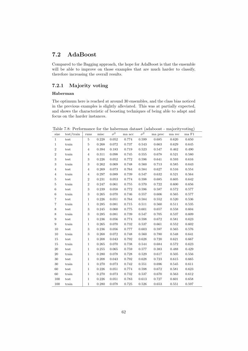
7.2 AdaBoost

Compared to the Bagging approach, the hope for AdaBoost is that the ensemblewill be able to improve on those examples that are much harder to classify,therefore increasing the overall results.


Haberman

The optimum here is reached at around 30 ensembles, and the class bias noticedin the previous examples is slightly alleviated. This was at partially expected,and shows the characteristic of boosting techniques of being able to adapt andfocus on the harder instances.

Table 7.8: Performance for the haberman dataset (adaboost - majorityvoting)size test/train runs misc σ2 ma acc σ2 ma prec ma rec ma F1

1 test 5 0.228 0.052 0.774 0.599 0.685 0.620 0.650

1 train 5 0.268 0.072 0.737 0.543 0.663 0.629 0.645

2 test 4 0.394 0.183 0.719 0.523 0.547 0.462 0.490

2 train 4 0.311 0.098 0.745 0.555 0.678 0.521 0.580

3 test 3 0.226 0.052 0.772 0.596 0.641 0.593 0.616

3 train 3 0.262 0.069 0.748 0.560 0.713 0.585 0.643

4 test 4 0.269 0.073 0.764 0.584 0.627 0.516 0.554

4 train 4 0.297 0.089 0.739 0.547 0.632 0.521 0.564

5 test 2 0.231 0.053 0.774 0.598 0.685 0.605 0.642

5 train 2 0.247 0.061 0.755 0.570 0.722 0.600 0.656

6 test 3 0.239 0.058 0.772 0.596 0.587 0.572 0.577

6 train 3 0.265 0.070 0.746 0.557 0.606 0.565 0.577

7 test 1 0.226 0.051 0.764 0.584 0.552 0.520 0.536

7 train 1 0.285 0.081 0.715 0.511 0.560 0.511 0.535

8 test 3 0.245 0.060 0.775 0.601 0.657 0.558 0.604

8 train 3 0.285 0.081 0.739 0.547 0.705 0.537 0.609

9 test 1 0.236 0.056 0.774 0.598 0.672 0.581 0.623

9 train 1 0.265 0.070 0.732 0.537 0.661 0.552 0.602

10 test 3 0.236 0.056 0.777 0.603 0.597 0.565 0.576

10 train 3 0.268 0.072 0.748 0.560 0.780 0.548 0.641

15 test 1 0.208 0.043 0.792 0.628 0.720 0.621 0.667

15 train 1 0.265 0.070 0.738 0.544 0.684 0.572 0.623

20 test 1 0.255 0.065 0.759 0.577 0.383 0.488 0.429

20 train 1 0.280 0.078 0.728 0.529 0.617 0.505 0.556

30 test 1 0.208 0.043 0.792 0.628 0.723 0.615 0.665

30 train 1 0.270 0.073 0.742 0.551 0.696 0.545 0.611

60 test 1 0.226 0.051 0.774 0.598 0.672 0.581 0.623

60 train 1 0.270 0.073 0.732 0.537 0.670 0.563 0.612

100 test 1 0.226 0.051 0.783 0.613 0.727 0.601 0.658

100 train 1 0.280 0.078 0.725 0.526 0.653 0.551 0.597

62

0.2

0.3

0.4

0.5

0.6

0.7

0.8

0 10 20 30 40 50 60 70 80 90 100

err

or

ensemble size

test error measurements (haberman-adaboost-majorityvoting)


m.a. recall

0

0.1

0.2

0.3

0.4

0.5

0.6

0.7

0 10 20 30 40 50 60 70 80 90 100

var(

x)

ensemble size

test error variance (haberman-adaboost-majorityvoting)


m.a. recall

Figure 7.24: Performance on the Haberman dataset (test set) for Bagging withMajority Voting

0.2

0.3

0.4

0.5

0.6

0.7

0.8

0 10 20 30 40 50 60 70 80 90 100

err

or

ensemble size

train error measurements (haberman-adaboost-majorityvoting)


m.a. recall

0

0.1

0.2

0.3

0.4

0.5

0.6

0.7

0 10 20 30 40 50 60 70 80 90 100

var(

x)

ensemble size

train error variance (haberman-adaboost-majorityvoting)


m.a. recall

Figure 7.25: Performance on the Haberman dataset (training set) for Baggingwith Majority Voting

0

10

20

30

40

50

60

70

80

0 1

count

class

test class bias for ensemble size 1 (haberman-adaboost-majorityvoting)

tptnfpfn

0

10

20

30

40

50

60

70

80

0 1

count

class

test class bias for ensemble size 10 (haberman-adaboost-majorityvoting)

tptnfpfn

Figure 7.26: Class bias on the Haberman dataset (test set) for Bagging withMajority Voting

Letter Recognition

Very similar observations can be made as the previous examples. It is likely thatthis is because the letter recognition dataset does not have a large number of

63

”hard” examples compared to the size of the dataset itself. It is remarkable howin this case the graphs resemble the ones obtained with bagging and majorityvoting, so they are included for comparison.

Table 7.9: Performance for the letterrecognition dataset (adaboost - majori-tyvoting)size test/train runs misc σ2 ma acc σ2 ma prec ma rec ma F1

1 test 4 0.480 0.235 0.979 0.958 0.849 0.550 0.664

1 train 4 0.459 0.216 0.980 0.960 0.868 0.568 0.684

2 test 4 0.519 0.274 0.979 0.959 0.918 0.488 0.635

2 train 4 0.502 0.257 0.980 0.960 0.933 0.502 0.650

3 test 3 0.476 0.233 0.980 0.961 0.891 0.535 0.666

3 train 3 0.457 0.216 0.981 0.962 0.901 0.551 0.681

4 test 3 0.507 0.263 0.979 0.959 0.896 0.502 0.642

4 train 3 0.486 0.242 0.980 0.961 0.917 0.519 0.661

5 test 2 0.504 0.262 0.979 0.959 0.887 0.508 0.643

5 train 2 0.483 0.242 0.980 0.961 0.910 0.524 0.662

6 test 3 0.503 0.260 0.980 0.960 0.886 0.506 0.642

6 train 3 0.482 0.240 0.981 0.962 0.910 0.523 0.661

7 test 2 0.499 0.254 0.980 0.960 0.902 0.511 0.650

7 train 2 0.477 0.234 0.981 0.961 0.924 0.529 0.670

8 test 2 0.513 0.270 0.979 0.959 0.914 0.496 0.639

8 train 2 0.494 0.251 0.980 0.961 0.930 0.510 0.656

9 test 2 0.502 0.258 0.980 0.960 0.885 0.509 0.644

9 train 2 0.480 0.237 0.980 0.961 0.900 0.527 0.662

10 test 3 0.483 0.240 0.980 0.961 0.908 0.528 0.665

10 train 3 0.465 0.223 0.981 0.963 0.929 0.542 0.681

15 test 1 0.581 0.338 0.977 0.954 0.856 0.427 0.569

15 train 1 0.562 0.315 0.977 0.955 0.892 0.443 0.592

20 test 2 0.506 0.263 0.979 0.959 0.897 0.503 0.642

20 train 2 0.485 0.242 0.980 0.961 0.918 0.521 0.662

30 test 2 0.505 0.262 0.979 0.959 0.892 0.504 0.641

30 train 2 0.484 0.241 0.980 0.961 0.918 0.521 0.661

60 test 1 0.586 0.344 0.977 0.954 0.856 0.422 0.565

60 train 1 0.566 0.320 0.977 0.955 0.937 0.438 0.597

100 test 1 0.591 0.350 0.976 0.953 0.854 0.416 0.559

100 train 1 0.569 0.323 0.977 0.955 0.938 0.435 0.594

64

0.4

0.5

0.6

0.7

0.8

0.9

1

0 10 20 30 40 50 60 70 80 90 100

err

or

ensemble size

test error measurements (letterrecognition-adaboost-majorityvoting)


m.a. recall

0.1

0.2

0.3

0.4

0.5

0.6

0.7

0.8

0.9

1

0 10 20 30 40 50 60 70 80 90 100

var(

x)

ensemble size

test error variance (letterrecognition-adaboost-majorityvoting)


m.a. recall

Figure 7.27: Performance on the Letter Recognition dataset (test set) for Bag-ging with Majority Voting

0.4

0.5

0.6

0.7

0.8

0.9

1

0 10 20 30 40 50 60 70 80 90 100

err

or

ensemble size

train error measurements (letterrecognition-adaboost-majorityvoting)


m.a. recall

0.1

0.2

0.3

0.4

0.5

0.6

0.7

0.8

0.9

1

0 10 20 30 40 50 60 70 80 90 100

var(

x)

ensemble size

train error variance (letterrecognition-adaboost-majorityvoting)


m.a. recall

Figure 7.28: Performance on the Letter Recognition dataset (training set) forBagging with Majority Voting

0

500

1000

1500

2000

2500

3000

3500

4000


count

class

test class bias for ensemble size 1 (letterrecognition-adaboost-majorityvoting)

tptnfpfn

0

500

1000

1500

2000

2500

3000

3500

4000


count

class

test class bias for ensemble size 10 (letterrecognition-adaboost-majorityvoting)

tptnfpfn

Figure 7.29: Class bias on the Letter Recognition dataset (test set) for Baggingwith Majority Voting

Landsat

With fewer than 10 members there there is good performance in general (forthis data set), but this seems to get worse with more members. The class bias

65

found with bagging is slightly alleviated, but not by much. Nevertheless thissmall improvement shows again that boosting techniques are able to correcterrors on difficult data.

Table 7.10: Performance for the landsat dataset (adaboost - majorityvoting)size test/train runs misc σ2 ma acc σ2 ma prec ma rec ma F1

1 test 3 0.452 0.218 0.925 0.855 0.551 0.435 0.486

1 train 3 0.390 0.164 0.933 0.872 0.565 0.460 0.506

2 test 3 0.482 0.248 0.925 0.856 0.622 0.418 0.499

2 train 3 0.416 0.185 0.934 0.873 0.607 0.444 0.512

3 test 1 0.615 0.379 0.907 0.823 0.526 0.327 0.403

3 train 1 0.547 0.299 0.918 0.842 0.493 0.351 0.410

4 test 3 0.473 0.238 0.926 0.858 0.576 0.420 0.485

4 train 3 0.414 0.188 0.934 0.873 0.579 0.449 0.505

5 test 3 0.447 0.216 0.928 0.861 0.562 0.438 0.492

5 train 3 0.386 0.164 0.936 0.877 0.579 0.465 0.515

6 test 2 0.517 0.288 0.920 0.847 0.527 0.398 0.453

6 train 2 0.441 0.211 0.931 0.866 0.537 0.424 0.474

7 test 2 0.486 0.253 0.925 0.855 0.598 0.409 0.484

7 train 2 0.429 0.199 0.932 0.870 0.548 0.433 0.484

8 test 2 0.494 0.256 0.923 0.853 0.596 0.412 0.487

8 train 2 0.415 0.181 0.934 0.872 0.599 0.441 0.507

9 test 3 0.433 0.200 0.931 0.866 0.616 0.449 0.519

9 train 3 0.371 0.148 0.939 0.881 0.615 0.475 0.536

10 test 2 0.503 0.272 0.923 0.852 0.533 0.396 0.454

10 train 2 0.446 0.217 0.931 0.867 0.542 0.422 0.474

15 test 1 0.595 0.354 0.911 0.830 0.531 0.342 0.416

15 train 1 0.518 0.269 0.921 0.849 0.519 0.364 0.428

20 test 2 0.514 0.287 0.920 0.847 0.594 0.404 0.479

20 train 2 0.433 0.204 0.931 0.868 0.593 0.431 0.498

30 test 1 0.622 0.387 0.908 0.824 0.535 0.328 0.407

30 train 1 0.532 0.283 0.920 0.847 0.538 0.354 0.427

60 test 1 0.589 0.347 0.913 0.834 0.538 0.346 0.421

60 train 1 0.512 0.262 0.923 0.852 0.539 0.367 0.437

100 test 1 0.594 0.353 0.912 0.831 0.535 0.344 0.419

100 train 1 0.511 0.261 0.923 0.852 0.535 0.368 0.436

66

0.3

0.4

0.5

0.6

0.7

0.8

0.9

1

0 10 20 30 40 50 60 70 80 90 100

err

or

ensemble size

test error measurements (landsat-adaboost-majorityvoting)


m.a. recall

0.1

0.2

0.3

0.4

0.5

0.6

0.7

0.8

0.9

0 10 20 30 40 50 60 70 80 90 100

var(

x)

ensemble size

test error variance (landsat-adaboost-majorityvoting)


m.a. recall

Figure 7.30: Performance on the Landsat dataset (test set) for Bagging withMajority Voting

0.3

0.4

0.5

0.6

0.7

0.8

0.9

1

0 10 20 30 40 50 60 70 80 90 100

err

or

ensemble size

train error measurements (landsat-adaboost-majorityvoting)


m.a. recall

0.1

0.2

0.3

0.4

0.5

0.6

0.7

0.8

0.9

0 10 20 30 40 50 60 70 80 90 100

var(

x)

ensemble size

train error variance (landsat-adaboost-majorityvoting)


m.a. recall

Figure 7.31: Performance on the Landsat dataset (training set) for Baggingwith Majority Voting

0

200

400

600

800

1000

1200

1400

1600

0 1 2 3 4 5 6

count

class

test class bias for ensemble size 1 (landsat-adaboost-majorityvoting)

tptnfpfn

0

200

400

600

800

1000

1200

1400

1600

0 1 2 3 4 5 6

count

class

test class bias for ensemble size 10 (landsat-adaboost-majorityvoting)

tptnfpfn

Figure 7.32: Class bias on the Landsat dataset (test set) for Bagging withMajority Voting

Magic

Despite the considerations about overfitting of data on this dataset, boostingtechniques are able to recover at least partially. Measurements seem to improve

67

almost monotonically with ensemble size, and this can be attributed to thecombination of increased variance (due to the higher number and complexity ofclassifiers) and the ”specialization” approach of boosting. Class bias diagramshave been omitted for this benchmark as there are no remarkable observationsto be made in comparison with prevoius benchmarks on the same set.

Table 7.11: Performance for the magic dataset (adaboost - majorityvoting)size test/train runs misc σ2 ma acc σ2 ma prec ma rec ma F1

1 test 2 0.493 0.245 0.518 0.270 0.500 0.264 0.345

1 train 2 0.132 0.017 0.870 0.756 0.862 0.750 0.802

2 test 1 0.493 0.243 0.545 0.297 0.500 0.254 0.337

2 train 1 0.143 0.020 0.872 0.760 0.882 0.733 0.801

3 test 2 0.485 0.235 0.524 0.274 0.500 0.261 0.343

3 train 2 0.134 0.018 0.868 0.754 0.858 0.746 0.798

4 test 2 0.492 0.242 0.529 0.279 0.500 0.254 0.337

4 train 2 0.137 0.019 0.871 0.758 0.872 0.738 0.799

5 test 2 0.477 0.227 0.532 0.283 0.500 0.267 0.348

5 train 2 0.131 0.017 0.870 0.757 0.860 0.751 0.802

6 test 2 0.474 0.225 0.540 0.291 0.500 0.264 0.345

6 train 2 0.134 0.018 0.871 0.759 0.870 0.744 0.802

7 test 2 0.472 0.223 0.537 0.288 0.500 0.267 0.349

7 train 2 0.132 0.017 0.871 0.758 0.863 0.750 0.802

8 test 1 0.490 0.240 0.524 0.274 0.500 0.255 0.338

8 train 1 0.134 0.018 0.870 0.757 0.866 0.742 0.799

9 test 1 0.469 0.220 0.536 0.287 0.500 0.268 0.349

9 train 1 0.130 0.017 0.872 0.760 0.863 0.752 0.804

20 test 1 0.474 0.225 0.532 0.283 0.500 0.264 0.346

20 train 1 0.132 0.017 0.870 0.757 0.862 0.748 0.801

0.25

0.3

0.35

0.4

0.45

0.5

0.55

0 2 4 6 8 10 12 14 16 18 20

err

or

ensemble size

test error measurements (magic-adaboost-majorityvoting)


m.a. recall

0.05

0.1

0.15

0.2

0.25

0.3

0 2 4 6 8 10 12 14 16 18 20

var(

x)

ensemble size

test error variance (magic-adaboost-majorityvoting)


m.a. recall

Figure 7.33: Performance on the Magic dataset (test set) for Bagging withMajority Voting

68

0.1

0.2

0.3

0.4

0.5

0.6

0.7

0.8

0.9

0 2 4 6 8 10 12 14 16 18 20

err

or

ensemble size

train error measurements (magic-adaboost-majorityvoting)


m.a. recall

0

0.1

0.2

0.3

0.4

0.5

0.6

0.7

0.8

0 2 4 6 8 10 12 14 16 18 20

var(

x)

ensemble size

train error variance (magic-adaboost-majorityvoting)


m.a. recall

Figure 7.34: Performance on the Magic dataset (training set) for Bagging withMajority Voting

69

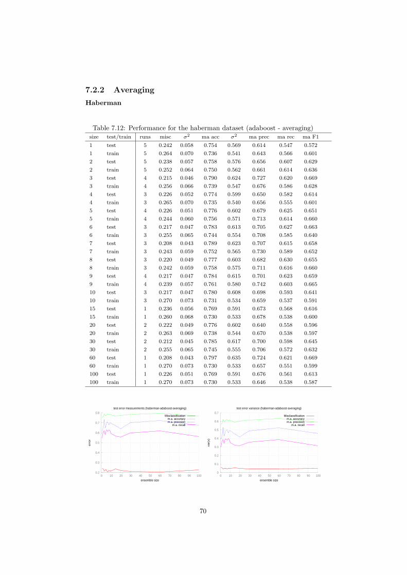
7.2.2 Averaging

Haberman

Table 7.12: Performance for the haberman dataset (adaboost - averaging)size test/train runs misc σ2 ma acc σ2 ma prec ma rec ma F1

1 test 5 0.242 0.058 0.754 0.569 0.614 0.547 0.572

1 train 5 0.264 0.070 0.736 0.541 0.643 0.566 0.601

2 test 5 0.238 0.057 0.758 0.576 0.656 0.607 0.629

2 train 5 0.252 0.064 0.750 0.562 0.661 0.614 0.636

3 test 4 0.215 0.046 0.790 0.624 0.727 0.620 0.669

3 train 4 0.256 0.066 0.739 0.547 0.676 0.586 0.628

4 test 3 0.226 0.052 0.774 0.599 0.650 0.582 0.614

4 train 3 0.265 0.070 0.735 0.540 0.656 0.555 0.601

5 test 4 0.226 0.051 0.776 0.602 0.679 0.625 0.651

5 train 4 0.244 0.060 0.756 0.571 0.713 0.614 0.660

6 test 3 0.217 0.047 0.783 0.613 0.705 0.627 0.663

6 train 3 0.255 0.065 0.744 0.554 0.708 0.585 0.640

7 test 3 0.208 0.043 0.789 0.623 0.707 0.615 0.658

7 train 3 0.243 0.059 0.752 0.565 0.730 0.589 0.652

8 test 3 0.220 0.049 0.777 0.603 0.682 0.630 0.655

8 train 3 0.242 0.059 0.758 0.575 0.711 0.616 0.660

9 test 4 0.217 0.047 0.784 0.615 0.701 0.623 0.659

9 train 4 0.239 0.057 0.761 0.580 0.742 0.603 0.665

10 test 3 0.217 0.047 0.780 0.608 0.698 0.593 0.641

10 train 3 0.270 0.073 0.731 0.534 0.659 0.537 0.591

15 test 1 0.236 0.056 0.769 0.591 0.673 0.568 0.616

15 train 1 0.260 0.068 0.730 0.533 0.678 0.538 0.600

20 test 2 0.222 0.049 0.776 0.602 0.640 0.558 0.596

20 train 2 0.263 0.069 0.738 0.544 0.670 0.538 0.597

30 test 2 0.212 0.045 0.785 0.617 0.700 0.598 0.645

30 train 2 0.255 0.065 0.745 0.555 0.706 0.572 0.632

60 test 1 0.208 0.043 0.797 0.635 0.724 0.621 0.669

60 train 1 0.270 0.073 0.730 0.533 0.657 0.551 0.599

100 test 1 0.226 0.051 0.769 0.591 0.676 0.561 0.613

100 train 1 0.270 0.073 0.730 0.533 0.646 0.538 0.587

0.2

0.3

0.4

0.5

0.6

0.7

0.8

0 10 20 30 40 50 60 70 80 90 100

err

or

ensemble size

test error measurements (haberman-adaboost-averaging)


m.a. recall

0

0.1

0.2

0.3

0.4

0.5

0.6

0.7

0 10 20 30 40 50 60 70 80 90 100

var(

x)

ensemble size

test error variance (haberman-adaboost-averaging)


m.a. recall

70

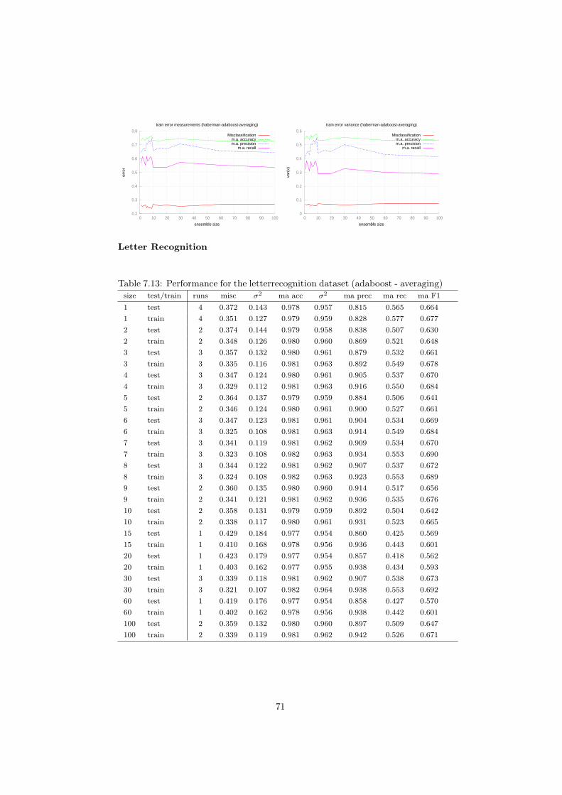
0.2

0.3

0.4

0.5

0.6

0.7

0.8

0 10 20 30 40 50 60 70 80 90 100

err

or

ensemble size

train error measurements (haberman-adaboost-averaging)


m.a. recall

0

0.1

0.2

0.3

0.4

0.5

0.6

0 10 20 30 40 50 60 70 80 90 100

var(

x)

ensemble size

train error variance (haberman-adaboost-averaging)


m.a. recall

Letter Recognition

Table 7.13: Performance for the letterrecognition dataset (adaboost - averaging)size test/train runs misc σ2 ma acc σ2 ma prec ma rec ma F1

1 test 4 0.372 0.143 0.978 0.957 0.815 0.565 0.664

1 train 4 0.351 0.127 0.979 0.959 0.828 0.577 0.677

2 test 2 0.374 0.144 0.979 0.958 0.838 0.507 0.630

2 train 2 0.348 0.126 0.980 0.960 0.869 0.521 0.648

3 test 3 0.357 0.132 0.980 0.961 0.879 0.532 0.661

3 train 3 0.335 0.116 0.981 0.963 0.892 0.549 0.678

4 test 3 0.347 0.124 0.980 0.961 0.905 0.537 0.670

4 train 3 0.329 0.112 0.981 0.963 0.916 0.550 0.684

5 test 2 0.364 0.137 0.979 0.959 0.884 0.506 0.641

5 train 2 0.346 0.124 0.980 0.961 0.900 0.527 0.661

6 test 3 0.347 0.123 0.981 0.961 0.904 0.534 0.669

6 train 3 0.325 0.108 0.981 0.963 0.914 0.549 0.684

7 test 3 0.341 0.119 0.981 0.962 0.909 0.534 0.670

7 train 3 0.323 0.108 0.982 0.963 0.934 0.553 0.690

8 test 3 0.344 0.122 0.981 0.962 0.907 0.537 0.672

8 train 3 0.324 0.108 0.982 0.963 0.923 0.553 0.689

9 test 2 0.360 0.135 0.980 0.960 0.914 0.517 0.656

9 train 2 0.341 0.121 0.981 0.962 0.936 0.535 0.676

10 test 2 0.358 0.131 0.979 0.959 0.892 0.504 0.642

10 train 2 0.338 0.117 0.980 0.961 0.931 0.523 0.665

15 test 1 0.429 0.184 0.977 0.954 0.860 0.425 0.569

15 train 1 0.410 0.168 0.978 0.956 0.936 0.443 0.601

20 test 1 0.423 0.179 0.977 0.954 0.857 0.418 0.562

20 train 1 0.403 0.162 0.977 0.955 0.938 0.434 0.593

30 test 3 0.339 0.118 0.981 0.962 0.907 0.538 0.673

30 train 3 0.321 0.107 0.982 0.964 0.938 0.553 0.692

60 test 1 0.419 0.176 0.977 0.954 0.858 0.427 0.570

60 train 1 0.402 0.162 0.978 0.956 0.938 0.442 0.601

100 test 2 0.359 0.132 0.980 0.960 0.897 0.509 0.647

100 train 2 0.339 0.119 0.981 0.962 0.942 0.526 0.671

71

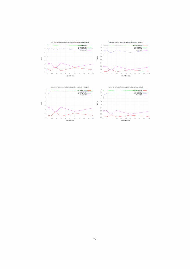
0.3

0.4

0.5

0.6

0.7

0.8

0.9

1

0 10 20 30 40 50 60 70 80 90 100

err

or

ensemble size

test error measurements (letterrecognition-adaboost-averaging)


m.a. recall

0.1

0.2

0.3

0.4

0.5

0.6

0.7

0.8

0.9

1

0 10 20 30 40 50 60 70 80 90 100

var(

x)

ensemble size

test error variance (letterrecognition-adaboost-averaging)


m.a. recall

0.3

0.4

0.5

0.6

0.7

0.8

0.9

1

0 10 20 30 40 50 60 70 80 90 100

err

or

ensemble size

train error measurements (letterrecognition-adaboost-averaging)


m.a. recall

0.1

0.2

0.3

0.4

0.5

0.6

0.7

0.8

0.9

1

0 10 20 30 40 50 60 70 80 90 100

var(

x)

ensemble size

train error variance (letterrecognition-adaboost-averaging)


m.a. recall

72

Landsat

Table 7.14: Performance for the landsat dataset (adaboost - averaging)size test/train runs misc σ2 ma acc σ2 ma prec ma rec ma F1

1 test 3 0.261 0.068 0.929 0.864 0.611 0.432 0.505

1 train 3 0.227 0.052 0.935 0.874 0.617 0.455 0.523

2 test 1 0.291 0.084 0.899 0.809 0.373 0.323 0.346

2 train 1 0.267 0.072 0.914 0.836 0.398 0.344 0.369

3 test 3 0.253 0.065 0.929 0.863 0.614 0.442 0.513

3 train 3 0.224 0.051 0.939 0.881 0.622 0.472 0.536

4 test 3 0.261 0.069 0.930 0.865 0.618 0.436 0.510

4 train 3 0.233 0.055 0.936 0.877 0.582 0.460 0.514

5 test 2 0.256 0.066 0.931 0.867 0.598 0.431 0.501

5 train 2 0.231 0.054 0.937 0.878 0.600 0.459 0.520

6 test 1 0.295 0.087 0.911 0.830 0.532 0.341 0.416

6 train 1 0.264 0.070 0.921 0.849 0.518 0.363 0.427

7 test 3 0.253 0.064 0.932 0.869 0.622 0.441 0.515

7 train 3 0.224 0.051 0.937 0.878 0.622 0.464 0.530

8 test 1 0.289 0.084 0.908 0.824 0.532 0.333 0.409

8 train 1 0.262 0.069 0.919 0.845 0.507 0.355 0.418

9 test 2 0.257 0.067 0.924 0.855 0.594 0.414 0.486

9 train 2 0.231 0.054 0.933 0.872 0.596 0.441 0.506

10 test 2 0.270 0.073 0.929 0.864 0.594 0.432 0.500

10 train 2 0.240 0.058 0.936 0.877 0.597 0.454 0.515

15 test 1 0.288 0.083 0.915 0.838 0.529 0.367 0.433

15 train 1 0.261 0.068 0.928 0.860 0.534 0.394 0.454

20 test 2 0.259 0.068 0.929 0.864 0.596 0.430 0.499

20 train 2 0.231 0.054 0.937 0.878 0.600 0.456 0.518

30 test 1 0.286 0.082 0.914 0.835 0.532 0.356 0.426

30 train 1 0.259 0.067 0.924 0.853 0.533 0.373 0.439

60 test 2 0.263 0.070 0.927 0.860 0.596 0.422 0.493

60 train 2 0.234 0.055 0.935 0.875 0.600 0.447 0.512

100 test 1 0.291 0.085 0.911 0.830 0.533 0.345 0.419

100 train 1 0.262 0.068 0.922 0.851 0.530 0.368 0.434

0.2

0.3

0.4

0.5

0.6

0.7

0.8

0.9

1

0 10 20 30 40 50 60 70 80 90 100

err

or

ensemble size

test error measurements (landsat-adaboost-averaging)


m.a. recall

0

0.1

0.2

0.3

0.4

0.5

0.6

0.7

0.8

0.9

0 10 20 30 40 50 60 70 80 90 100

var(

x)

ensemble size

test error variance (landsat-adaboost-averaging)


m.a. recall

73

0.2

0.3

0.4

0.5

0.6

0.7

0.8

0.9

1

0 10 20 30 40 50 60 70 80 90 100

err

or

ensemble size

train error measurements (landsat-adaboost-averaging)


m.a. recall

0

0.1

0.2

0.3

0.4

0.5

0.6

0.7

0.8

0.9

0 10 20 30 40 50 60 70 80 90 100

var(

x)

ensemble size

train error variance (landsat-adaboost-averaging)


m.a. recall

74

Magic

7.3 Stacking

7.3.1 MetaClassifier

Haberman

Table 7.15: Performance for the landsat dataset (stacking - metaclassifier-mlp30-0.07)size test/train runs misc σ2 ma acc σ2 ma prec ma rec ma F1

1 test 1 0.606 0.368 0.883 0.780 0.327 0.313 0.320

1 train 1 0.462 0.214 0.904 0.817 0.350 0.318 0.333

2 test 1 0.810 0.656 0.860 0.740 0.146 0.266 0.189

2 train 1 0.648 0.420 0.887 0.787 0.203 0.273 0.233

3 test 1 0.813 0.660 0.791 0.625 0.128 0.271 0.174

3 train 1 0.651 0.423 0.835 0.696 0.176 0.275 0.214

4 test 1 0.814 0.662 0.795 0.631 0.156 0.264 0.196

4 train 1 0.655 0.429 0.835 0.698 0.185 0.268 0.219

5 test 1 0.814 0.662 0.769 0.591 0.151 0.264 0.192

5 train 1 0.656 0.431 0.813 0.662 0.177 0.269 0.214

6 test 1 0.819 0.670 0.772 0.595 0.164 0.243 0.196

6 train 1 0.664 0.441 0.814 0.663 0.182 0.250 0.210

7 test 1 0.816 0.666 0.781 0.609 0.163 0.258 0.200

7 train 1 0.657 0.432 0.823 0.678 0.183 0.261 0.216

8 test 1 0.822 0.676 0.765 0.585 0.163 0.250 0.197

8 train 1 0.669 0.447 0.809 0.654 0.180 0.256 0.211

9 test 1 0.858 0.736 0.759 0.576 0.020 0.143 0.035

9 train 1 0.728 0.529 0.795 0.632 0.037 0.143 0.059

10 test 1 0.822 0.675 0.766 0.586 0.163 0.238 0.193

10 train 1 0.667 0.445 0.810 0.656 0.180 0.248 0.209

15 test 1 0.819 0.670 0.769 0.592 0.163 0.251 0.198

15 train 1 0.663 0.440 0.813 0.660 0.180 0.258 0.212

20 test 1 0.868 0.753 0.803 0.645 0.029 0.143 0.049

20 train 1 0.766 0.587 0.835 0.698 0.054 0.143 0.078

30 test 1 0.868 0.753 0.760 0.578 0.020 0.143 0.035

30 train 1 0.766 0.587 0.789 0.623 0.035 0.143 0.057

60 test 1 0.852 0.726 0.865 0.748 0.100 0.105 0.103

60 train 1 0.750 0.562 0.879 0.773 0.121 0.114 0.118

100 test 1 0.868 0.753 0.752 0.566 0.019 0.143 0.033

100 train 1 0.766 0.587 0.781 0.610 0.033 0.143 0.054

75

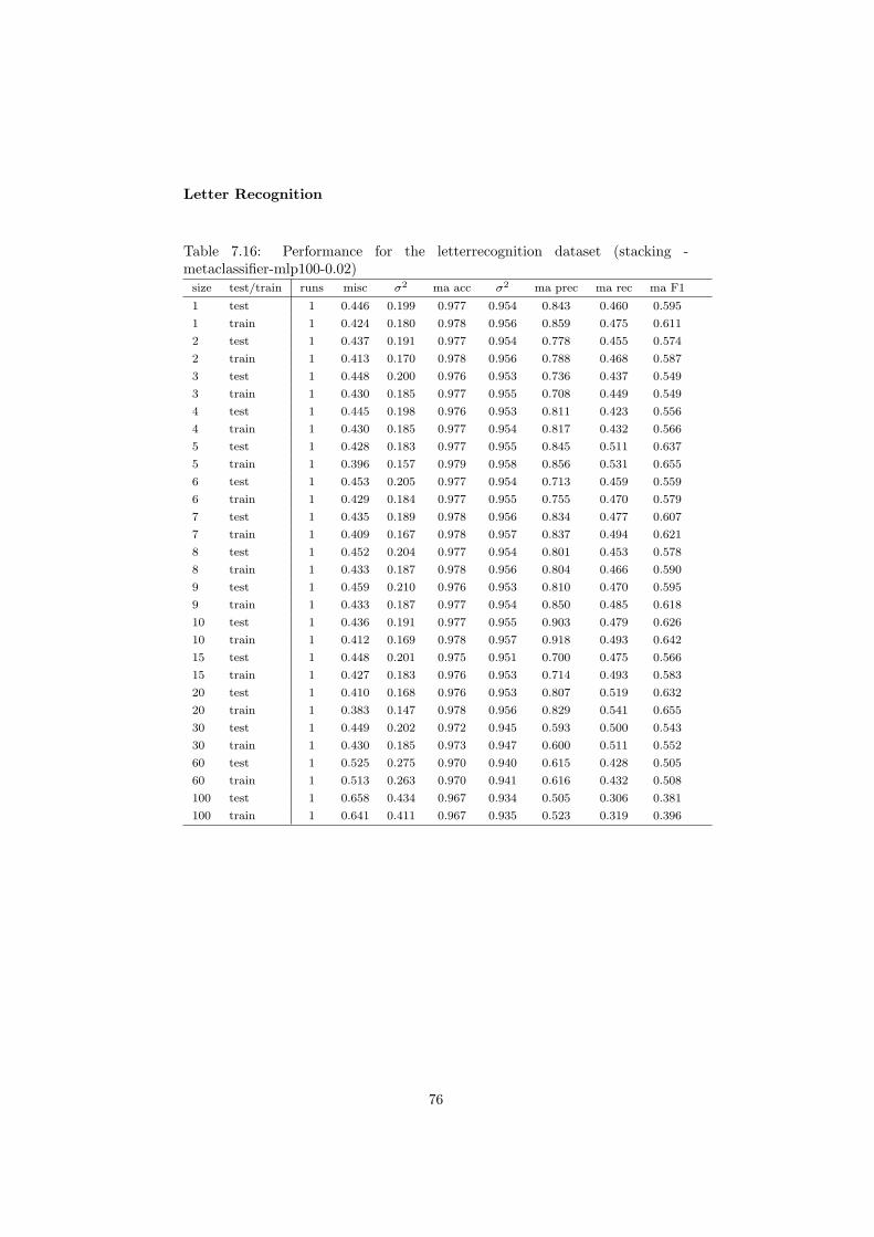
Letter Recognition

Table 7.16: Performance for the letterrecognition dataset (stacking -metaclassifier-mlp100-0.02)size test/train runs misc σ2 ma acc σ2 ma prec ma rec ma F1

1 test 1 0.446 0.199 0.977 0.954 0.843 0.460 0.595

1 train 1 0.424 0.180 0.978 0.956 0.859 0.475 0.611

2 test 1 0.437 0.191 0.977 0.954 0.778 0.455 0.574

2 train 1 0.413 0.170 0.978 0.956 0.788 0.468 0.587

3 test 1 0.448 0.200 0.976 0.953 0.736 0.437 0.549

3 train 1 0.430 0.185 0.977 0.955 0.708 0.449 0.549

4 test 1 0.445 0.198 0.976 0.953 0.811 0.423 0.556

4 train 1 0.430 0.185 0.977 0.954 0.817 0.432 0.566

5 test 1 0.428 0.183 0.977 0.955 0.845 0.511 0.637

5 train 1 0.396 0.157 0.979 0.958 0.856 0.531 0.655

6 test 1 0.453 0.205 0.977 0.954 0.713 0.459 0.559

6 train 1 0.429 0.184 0.977 0.955 0.755 0.470 0.579

7 test 1 0.435 0.189 0.978 0.956 0.834 0.477 0.607

7 train 1 0.409 0.167 0.978 0.957 0.837 0.494 0.621

8 test 1 0.452 0.204 0.977 0.954 0.801 0.453 0.578

8 train 1 0.433 0.187 0.978 0.956 0.804 0.466 0.590

9 test 1 0.459 0.210 0.976 0.953 0.810 0.470 0.595

9 train 1 0.433 0.187 0.977 0.954 0.850 0.485 0.618

10 test 1 0.436 0.191 0.977 0.955 0.903 0.479 0.626

10 train 1 0.412 0.169 0.978 0.957 0.918 0.493 0.642

15 test 1 0.448 0.201 0.975 0.951 0.700 0.475 0.566

15 train 1 0.427 0.183 0.976 0.953 0.714 0.493 0.583

20 test 1 0.410 0.168 0.976 0.953 0.807 0.519 0.632

20 train 1 0.383 0.147 0.978 0.956 0.829 0.541 0.655

30 test 1 0.449 0.202 0.972 0.945 0.593 0.500 0.543

30 train 1 0.430 0.185 0.973 0.947 0.600 0.511 0.552

60 test 1 0.525 0.275 0.970 0.940 0.615 0.428 0.505

60 train 1 0.513 0.263 0.970 0.941 0.616 0.432 0.508

100 test 1 0.658 0.434 0.967 0.934 0.505 0.306 0.381

100 train 1 0.641 0.411 0.967 0.935 0.523 0.319 0.396

76

Landsat

Table 7.17: Performance for the landsat dataset (stacking - metaclassifier-mlp30-0.07)size test/train runs misc σ2 ma acc σ2 ma prec ma rec ma F1

1 test 1 0.606 0.368 0.883 0.780 0.327 0.313 0.320

1 train 1 0.462 0.214 0.904 0.817 0.350 0.318 0.333

2 test 1 0.810 0.656 0.860 0.740 0.146 0.266 0.189

2 train 1 0.648 0.420 0.887 0.787 0.203 0.273 0.233

3 test 1 0.813 0.660 0.791 0.625 0.128 0.271 0.174

3 train 1 0.651 0.423 0.835 0.696 0.176 0.275 0.214

4 test 1 0.814 0.662 0.795 0.631 0.156 0.264 0.196

4 train 1 0.655 0.429 0.835 0.698 0.185 0.268 0.219

5 test 1 0.814 0.662 0.769 0.591 0.151 0.264 0.192

5 train 1 0.656 0.431 0.813 0.662 0.177 0.269 0.214

6 test 1 0.819 0.670 0.772 0.595 0.164 0.243 0.196

6 train 1 0.664 0.441 0.814 0.663 0.182 0.250 0.210

7 test 1 0.816 0.666 0.781 0.609 0.163 0.258 0.200

7 train 1 0.657 0.432 0.823 0.678 0.183 0.261 0.216

8 test 1 0.822 0.676 0.765 0.585 0.163 0.250 0.197

8 train 1 0.669 0.447 0.809 0.654 0.180 0.256 0.211

9 test 1 0.858 0.736 0.759 0.576 0.020 0.143 0.035

9 train 1 0.728 0.529 0.795 0.632 0.037 0.143 0.059

10 test 1 0.822 0.675 0.766 0.586 0.163 0.238 0.193

10 train 1 0.667 0.445 0.810 0.656 0.180 0.248 0.209

15 test 1 0.819 0.670 0.769 0.592 0.163 0.251 0.198

15 train 1 0.663 0.440 0.813 0.660 0.180 0.258 0.212

20 test 1 0.868 0.753 0.803 0.645 0.029 0.143 0.049

20 train 1 0.766 0.587 0.835 0.698 0.054 0.143 0.078

30 test 1 0.868 0.753 0.760 0.578 0.020 0.143 0.035

30 train 1 0.766 0.587 0.789 0.623 0.035 0.143 0.057

60 test 1 0.852 0.726 0.865 0.748 0.100 0.105 0.103

60 train 1 0.750 0.562 0.879 0.773 0.121 0.114 0.118

100 test 1 0.868 0.753 0.752 0.566 0.019 0.143 0.033

100 train 1 0.766 0.587 0.781 0.610 0.033 0.143 0.054

Magic

77

Chapter 8

Discussion, Conclusions andFurther Work

This empirical sampling of the performance of different ensemble techniquesleads to some interesting, and perhaps not very surprising, observations. Ingeneral these are mostly confirmations of concepts that are already known aboutensemble learning.

8.1 Validity of results

One thing that needs to be considered is that the limited amount of datasetsused is very small and certainly not sufficient to consider any results as proof,but they are certainly an indicator of the performance improvements that couldbe achieved with more sofisticated machine learning techniques.

8.2 Efficiency

The efficiency of training ensemble solutions, especially when the techniqueinvolves sequential training of each member, is something that needs to beconsidered when picking ensemble techniques. The time required for trainingtends to grow proportionally to the size of the ensemble and the complexityof the architecture. This is especially true when considering online training ofensemble techniques.

8.3 Noise

Another benefit that can be observed is the reduction of noise in the classificationdecisions over repeated tests. Intuitively we can imagine that when there aremany components that need to reach an agreement it is less likely that therewill be many outliers.

78

8.4 Different datasets have different results

It is evident from observation of the results that different datasets will producevaried results, this is mainly due to the fact that the multi layer perceptrons usedin the empirical tests might not be a good method for those specific datasets.Different datasets also have different applicability to an ensemble learning tech-nique, and generally we notice that datasets that require a ”deeper” learningseem to produce results that are not as good (but still better than the singleclassifier).

8.5 Further work

Although this was a very long project, the entirety of the work done in thisperiod is only scratching the surface of what else could be done.

8.5.1 Re-running benchmarks with different parameters

Despite the amount of care that has gone into the selection of parameters, ithas been found in a few cases that there was either underfitting or overfitting.It would be ideal, given the time, to repeat these tests with new parameters,and using alternative neural network architectures and ml techniques.

8.5.2 Further expansions to Encog

Regression

All these techniques have been implemented and studied with a regard towardsclassification problems. It should be sufficiently easy to adapt the source codeto support regression as well as classification. In some places I have alreadyinserted placeholders or comments for what could be done to achieve this, sothat before contributing my work back I can add this functionality.

Other techniques

The techniques implemented in this paper are not the only ensemble techniques.There are several others, all of which could be implemented taking advantageof the basic framework that I have put together. This is left as a further devel-opment by the community.

8.5.3 Contribution back to the community

Due to the time constraints, it was not possible to prepare the source code in theform of a patch that could be contributed back to the Encog community. Thisis a process that I intend to complete within a short time after the submissionof this document and all that is required is to produce a patch set that does notcontain any of the training experiments, as well as writing the relevant javadocentries and generic documentation.

79

8.5.4 Real-world use of Encog Ensembles

This study lacks coverage of real world applications on datasets that have notbeen already extensively used. Amongst future plans, I intend to validate the useof ensembles in Encog by applying some techniques to problems and competi-tions openly available. This should provide more tangible proof of the usefulnessof these methods.

80

Bibliography

[1] Vijaya Kumar B Al-Ghoneim K. Learning ranks with neural networks.Application and Science of Artificial Neural Networks: proceedinges of theSPIE, 2492:446–464, 1995.

[2] M Anthony and P Bartlett. Neural Network Learning: Theoretical Foun-dations. Cambridge University Press, 1999.

[3] R Beale and T Jackson. Neural Computing - an introduction. Institute ofPhysics Publishing, 1990.

[4] C Bishop. Neural Networks for Pattern Recognition. Oxford UniversityPress, 1995.

[5] C Bishop. Pattern Recognition and Machine Learning (Information Scienceand Statistics). Springer, 1 edition, 2007.

[6] R K Bock, A Chilingarian, A Gaug, M Hakl, F Hengstebeck, T Jirina,M Klaschka, J Kotrc, P Savicky, S Towers, A Vaicilius, and W Wittek.Methods for multidimensional event classification: a case study using im-ages from a cherenkov gamma-ray telescope. Nucl. Instr. Meth. A, 516:511–528, 2004.

[7] D Brain and G I Webb. On the effect of data set size on bias and variancein classification learning. Proceedings of the Fourth Australian KnowledgeAcquisition Workshop, pages 117–128, 1999.

[8] L. Breiman. Bagging predictors. Machine Learning, 24(2):123–140, 1996.

[9] Dasarathy B.V. and Sheela B.V. A composite classifier system design:Concepts and methodology. Proceedings of the IEEE, 67(5):708 – 713, may1979.

[10] S. Cho and J. Kim. Multiple network fusion using fuzzy logic. IEEETransactions on Neural Networks, 6(2):497 – 501, March 1995.

[11] Nguyen D and Widrow B. Improving the learning speed of 2-layer neu-ral networks by choosing initial values of the adaptive weights. IJCNNInternational Joint Conference on Neural Networks, pages 21–26, 1990.

[12] Opitz D and Shavlik J. Generating accurate and diverse members of aneural-network ensemble. NIPS, 8:535–541, 1996.

[13] Wolpert D. Stacked generalization. Neural Networks, 5:241–259, 1992.

81

[14] J Dvorak and P Savicky. Softening splits in decision trees using simulatedannealing. Proceedings of ICANNGA 2007, Warsaw, pages 721–729.

[15] P W Frey and D J Slate. Letter recognition using holland-style adaptiveclassifiers. Machine Learning, 6(2), March 1991.

[16] G. Fumera and F. Roli. Performance analysis and comparison of linearcombiners for classifier fusion. 2002.

[17] Giacinto G, Perdisci R, Del Rio M, and Roli F. Intrusion detection in com-puter networks by a modular ensemble of one class classifiers. InformationFusion, 2006.

[18] E Gamma, R Helm, R Johnson, and J Vlissides. Design Patterns: Elementsof Reusable Object-Oriented Software. Addison-Wesley, 1994.

[19] S Geman, E Bienenstock, and R Doursat. Neural networks and thebias/variance dilemma. Neural Computation, 4:1–48, 1992.

[20] X Giannakopoulos, J Karhunen, and E Oja. An experimental comparisonof neural algorithms for independent component analysis and blind sepa-ration. Int. J. Neural Syst, 9, 1999.

[21] C Goutte and E Gaussier. A probabilistic interpretation of precision, recalland f-score, with implication for evaluation. 2005.

[22] S J Haberman. Generalized residuals for log-linear models. Proceedings ofthe 9th Internation Biometrics Conference, Boston, pages 104–122, 1976.

[23] Srihari S Ho T, Hull J. Decision combination in multiple classifier systems.IEEE Transactions on Pattern Analysis and Machine Intelligence, 16:66–76, 1994.

[24] Chuanyi Ji and Sheng Ma. Combinations of weak classifiers. IEEE Trans-actions on Neural Networks, 8(1):32–42, January 1997.

[25] J Kittler, M Hatef, R Duin, and J Matas. On combining classifiers. IEEETransactions on pattern analisys and machine intelligence, 20(3):226 – 239,March 1998.

[26] L. Kuncheva. A theoretical study on six classifier fusion strategies. IEEETransactions on pattern analisys and machine intelligence, 24(2):281 – 286,February 2002.

[27] J M Landwehr, D Pregibon, and A C Shoemaker. Graphical models forassessing logistic regression models (with discussion). Journal of the Amer-ican Statistical Association, 79:61–83.

[28] S Lawrence, I Burns, A Back, A Chung Tsoi, and C L Giles. Neural NetworkClassification and Prior Class Probabilities, volume 1524. 1998.

[29] G Lera. Neighborhood based levenberg-marquardt algorithm for neuralnetwork training. 2002.

[30] W D Lo. Logistic Regression Trees. PhD thesis, University of Wisconsin,1993.

82

[31] CD Manning, P Raghavan, and H Schutze. Introduction to informationretrieval. Cambridge University Press, 2008.

[32] M Moller. A scaledconjugategradient algorithm for fast supervised learning.1993.

[33] Melville P and Mooney R. Creating diversity in ensembles using artificialdata. Information Fusion, 6:99–111, 2005.

[34] Quinlan R. Bagging, boosting, and c4.5. 2006.

[35] Yuval Raviv and Nathan Intrator. Bootstrapping with noise: An effectiveregularization technique. Connection Science, 8:355–372, 1996.

[36] M Riedmiller. Rprop - description and implementation details. 1994.

[37] R Rojas and J Feldman. Neural Networks: A Systematic Introduction.Prentice Hall, 1996.

[38] S Russell and P Norvig. Artificial Intelligence: A Modern Approach. Pren-tice Hall, 1998.

[39] P Savicky and E Kotrc. Experimental study of leaf confidences for randomforest. Proceedings of COMPSTAT 2004, In: Computational Statistics,pages 1767–1774, 2004.

[40] R. E. Schapire. The strength of weak learnability. Machine Learning,5:197–227, 1990.

[41] R. E. Schapire and Y Freund. Experiments with a new boosting algorithm.Machine Learning: proceedings of the Thirteenth International Conference,pages 148–156, 1996.

[42] R. E. Schapire and Y Freund. A decision-theoretic generalization of on-linelearning and an application to boosting. Journal of Computer and SystemSciences, 55(1):119–139, 1997.

[43] R E Schapire, Y Freund, P Bartlett, and W Sun Lee. Boosting the margin:A new explanation for the effectiveness of voting methods. 1998.

[44] R. E. Schapire, Y Freund, and R Iyer. An efficient boosting algorithmfor combining preferences. Machine Learning: proceedings of the FifteenthInternational Conference, 1998.

[45] K Tumer and J Ghosh. Robust combining of disparate classifiers throughorder statistics. Technical report, AT&T Labs, 1999.

[46] K Tumer and N C Oza. Decimated input ensembles for improved general-ization. Technical report, NASA Ames Research Center, 1999.

[47] Wikipedia. Precision and recall. http://en.wikipedia.org/wiki/Precision_and_recall,2012. [Online; Accessed Aug 31st, 2012].

[48] Shuang Yang and Antony Browne. Neural network ensembles: combiningmultiple models for enhanced performance using a multistage approach.Expert Systems, 21(5):279–288, November 2004.

83

http://en.wikipedia.org/wiki/Precision_and_recall

extending encog: a study on classiﬁer ensemble techniquesamosca02/pdfs/msc_thesis_final.pdf ·...

Documents