extended families and child well-being - colby · pdf fileextended families and child...
TRANSCRIPT

Extended Families and Child Well-being
Daniel LaFave Duke University
Duncan Thomas
Duke University
First Draft: October 2009 Current Draft: March 2012†
Abstract
This paper provides empirical evidence on whether and how resources controlled by extended family members affect child health, cognition, and education using uniquely rich longitudinal data from the Indonesia Family Life Survey (IFLS). The IFLS contains information on resources under the control of each individual within households, as well as resources of individual family members who are not co-resident. Using this data in the context of a theoretical model of family resource allocation that imposes few restrictions on preferences of individuals within a group, we provide direct empirical evidence on the role that intergenerational transfers play in human capital accumulation. Our results suggest departures from the traditional unitary model of the family, but we cannot rule out that co-resident and non co-resident family members make allocation decisions cooperatively. The results are important for understanding family behavior, intergenerational exchange, and child health and well-being.
† Financial support from the National Institute of Child Health and Human Development and the Hewlett Foundation is gratefully acknowledged. The paper has benefited from discussions with Joseph Hotz, Marjorie McElory, Bob Pollak, David Ribar, Seth Sanders, Alessandro Tarozzi, and numerous seminar participants. Corresponding author: Daniel LaFave, Box 90097 Department of Economics, Duke University, Durham, NC 27708. Email: [email protected]

2
1. Introduction
How intergenerational transfers affect child well-being and human capital accumulation is poorly
understood. Despite its importance, few data sets provide the information on resources under the
control of both co-resident and non co-resident family members necessary to examine sharing within
extended families. Even fewer data sets provide information that links the level and distribution of
resources in the extended family to child health and development outcomes. Using extremely rich
longitudinal data from the Indonesia Family Life Survey (IFLS), this chapter provides empirical evidence
on whether, and how, resources under the control of parents, grandparents, and other non co-resident
family members contribute to child development. Results are presented in the context of a general
model of family behavior that provides a natural, but previously unused, framework to examine how
human capital formation is influenced by intergenerational exchange and resource allocation.
There is a growing body of literature on the importance of the extended family in economic
models of decision making. This is particularly true in developing settings where nuclear, two adult
households are far less common than in the developed world.1 Living arrangements in developing
countries frequently consist of multi or skip generation households, and extended families often fill gaps
created by the absence of formal social safety nets.2 Previous studies across the social sciences suggest
that intergenerational transmission plays a particularly important role in establishing early life health and
well-being. The IFLS offers a rich design and set of outcomes to study this behavior, and we focus
specifically on three markers of human capital; health as captured by height-for-age, early school
attendance, and cognition.3
We examine the links between extended family resources and child well-being within the context
1 For work and evidence on the role and importance of the extended family in the United States, see Altonji et al. (1992), Cox (2003), and Bianchi et al. (2008) among many others. 2 Evidence on extended family interaction in developing countries can be found in many settings. For example: Botswana (Lucas and Stark, 1985); India (Rosenzweig and Stark, 1989); South Africa (Duflo, 2003); and Indonesia (Thomas and Frankenberg, 2007) among many others. 3 Work in nutrition (Waterlow et al., 1977) has long supported the use of height as an indicator of well-being, and a number of studies have shown it to be predictive of a multitude of later life outcomes (e.g. Alderman et al., 2006).

3
of models of family decision making. This is a unique application, as the intrahousehold literature
primarily focuses on consumption allocations of nuclear households and rarely considers the extended
family or health. The use of outcomes with distinct human capital interpretations give the results clear
welfare implications lacking from papers studying consumption patterns. We consider both the
neoclassical unitary model of the family, as well as Chiappori's (1988, 1992) collective rationality model.4
The later offers the least restrictive approach in the intrahousehold literature, and relies only on the
assumption that family members reach Pareto efficient outcomes when allocating resources. Although
very few studies have used this model to examine the extended family, it is an appealing approach, as it
permits heterogeneous preferences across family members and generations while placing plausible,
testable restrictions on the nature of interactions between relatives.
Where other studies have been limited by the lack of data on the distribution of resources both
within households and the extended family, this chapter benefits from the rich longitudinal panel of the
Indonesia Family Life Survey. The structure and tracking scheme of the survey allows one to identify
extended families in the data by linking individuals who split-off from baseline households back to their
original household of origin. Along with genealogical construction, the IFLS contains detailed health,
education, and cognition measures that are utilized to assess how resources within a child's family impact
their development.
The results show that children are impacted not only by the resources under control of their
parents, but also those held by extended family members. We also show that the extended family not
only influences child outcomes, but they do so in a way that is consistent with a cooperative group of
heterogeneous individuals who coordinate their behavior. The empirical results strongly reject the
unitary model as the appropriate framework for the extended family, but cannot rule out that families
allocate resources in a Pareto efficient manner. This results is important for the design and evaluation of
development policy, as well as understanding family behavior, child health, and intergenerational
4 A number of additional intrahousehold models exist in the literature including McElroy and Horney (1981) and Lundberg and Pollack (1993) among many others.

4
exchange. The next section begins by describing a general theoretical framework to structure the
analysis.
2. Theoretical Framework
Drawing on work by Chiappori and coauthors (e.g. Chiappori 1988, 1992 and Browning et al., 1994), the
following is a general model of extended family behavior that encompasses both the unitary and
collective forms. In this framework, the general welfare of an extended family is a function of the
individual utility of each of its members. Motivated by the literature on bargaining within households,
this general framework allows for an arbitrary bargaining process to occur between members of an
extended family as they make allocation decisions.
To begin, let the welfare of an extended family, W, depend on the utility of each of its M
members, where m = 1, ..., M. Each individual's utility, Um, is allowed to depend on their own
consumption and that of all other extended family members. Each consumption vector is denoted by
!km, k = 1,…,K, where k indexes goods, and !0m denotes leisure of member m. The vectors !km contain a
variety of goods, but specifically include health and human capital outcomes. We analyze conditional
demand functions related to human capital, and consider health and education directly as consumption
goods. This is not an unreasonable approach, as evidence suggests extended family members place great
emphasis on the health and well-being of their young children. The model allows one to remain agnostic
about the functional form of the utility functions, and only require standard assumptions that it be quasi-
concave, non-decreasing, and strictly increasing in at least one argument.
Individual utility is allowed to vary depending on individual, household, and dynasty specific
characteristics.5 Some of these characteristics, denoted as µ, are observed in our data, and include
variables such as age, household demographic structure, anthropometrics, and socioeconomic status.
Other characteristics which influence utility remain unobserved to the econometrician, and are denoted 5 We will use “dynasty” and “extended family” interchangeably throughout the paper.

5
by ". Such characteristics may include attitudes toward health investments and altruism. Each individual's
utility function is then defined as Um(!, µ, ").
The extended family welfare function, W, aggregates individual utilities with corresponding
weights given by the function #($, %). The weight an individual's utility receives within the extended
family depends on observed individual, household and dynasty characteristics, denoted by $, which may
include individual asset holdings, marriage market opportunities, age, prices, and the wealth of each
dynasty member. The weights may also depend on unobserved characteristics, %, such as time
preferences.6 The presence of the weighting function #( . ) incorporates the notion of an intra-dynasty
decision making process, and reflects each members’ power in influencing allocation decisions. One
advantage of this general model is that it is consistent with a variety of bargaining processes within the
extended family, allowing one to remain agnostic on the actual process within the dynasty including
whether one occurs. As we address further when discussing the collective model, the weights do not
have a direct impact on an individual's utility, but do place testable restrictions on how an individual's
bargaining power may affect decisions within the family.
As stated, the dynasty's problem is to maximize extended family welfare subject to a budget
constraint that requires the amount of dynasty expenditure to be less than or equal to the value of total
family assets and labor income. Formally, the family solves:
!"#$!
W[U1(!, µ, "), … , UM(!, µ, "), #($, %)] (1)
subject to:
p!! ! "m [ Am + p0m(T - !0m)] + A0 (2)
where Am are assets controlled by family member m, and A0 are assets jointly controlled by the dynasty.
6 In this specification, ! and % may include some factors that also influence preferences through µ and ".

6
Individual labor income is the product of an individual's wage, p0m, and labor hours, where T is the time
endowment. Dynasty expenditure is equal to spending on consumption goods and human capital across
all members, p!!.7,8
The above framework is general enough to encompass both the unitary and collective models of
extended family behavior. As the allocation patterns which result from the two frameworks provide the
theoretical basis for the remainder of the chapter, the conditional demand functions and testable
implications that stem from each of these models follow in the next sections.
2.1 Unitary Model
At the dynasty level, the unitary model is equivalent to either a model where all family members have the
same preferences or a dictator model where only one decision maker's preferences enter the welfare
function W (e.g. Samuelson, 1956 and Becker, 1981). When one imposes the restrictions of the unitary
model on the general framework, solving the extended family's maximization problem results in a
conditional demand equation for good k of the form:
!k =!k ( "m ym, p, !, ") (3)
where resources of member m, including assets and income, are given by ym, p is a vector of exogenous
prices, and µ and " are observed and unobserved characteristics. The key feature of equation (3) is that
individual resources enter the conditional demand function only through their part in the sum total of
family resources, "m ym. This is the common “income pooling” interpretation which offers clear testable
implication of the unitary model. In the extended family setting, the restriction implies that once we
control for total dynasty resources, the share under the control of a child's own household,
7 In this framework, savings may be thought of as spending on an investment good. 8 Although this is a static approach, there are potentially important implications of this model in dynamic settings. Considering a dynamic model is left for future work, and will be able to speak to insurance and consumption smoothing within extended families in an important way.

7
grandmother, father, aunt, or uncle should have no independent effect on allocation decisions. This is a
strong restriction which merits empirical examination.
Testable Implications of the Unitary Model
If the unitary model is valid, the resource distribution within the extended family is irrelevant. This is
empirically testable by examining whether the marginal effect of each member's resources on childhood
outcomes is the same regardless of whom we consider. For example, do resources under the control of
fathers and grandmothers have the same impact on child health? Letting family members be indexed as
m and n, in terms of equation (3), the theoretical predication is:
(4)
While this test has been undertaken in a variety of papers empirically assessing the validity of the
unitary framework at the household level, we choose to use an alternative specification.9 As only total
dynasty resources matter in the conditional demand function in (3), if one conditions on total family
resources, "m ym, the share controlled by any specific individual should have no impact on !. In terms of
equation (3), that is:
(5)
A full description of the empirical implementation of this testable restriction, its advantages, and
a discussion of results follow in later sections. We turn next to the collective framework, and discuss the
testable implications that follow from a more general model of family behavior.
9 See Horney and McElroy (1988), Schultz (1990), and Thomas (1990) among others for tests of the unitary model relying on restrictions similar to (4).
∂θk
∂ym=
∂θk
∂yn∀ k,m, n
∂θk
∂yn
���Pm ym
= 0 ∀ k, n

8
2.2 Collective Model
The unitary model provides a baseline for the analysis of extended families and child well-being.
However, if one rejects the unitary framework, the aforementioned tests do not immediately offer an
appropriate model of family behavior in its place. As a result, it is only natural to follow tests of the
unitary model with those derived from a more general alternative. The collective model relaxes the
common preferences or dictator assumptions of the unitary framework, and allows for sharing and
bargaining within families while maintaining that allocation decisions achieve Pareto efficient
outcomes.10
Income Sharing Approach
Browning and Chiappori (1998) show that the collective model is formally equivalent to a model where
families make allocation decisions in a two step process. In the first stage, resources are shared within
the family. Extended family members effectively pool their resources together and then distribute them
amongst each other with each member receiving a share determined by their relative power within the
dynasty. In the second stage, members make maximizing allocation decisions subject to the share of
resources they received in the first stage.
In this interpretation of the collective model, the fraction of total family resources a decision
maker receives is determined by a sharing rule related to the prevoiusly defined weighting function. The
sharing function depends on individual resources, prices, other observed and unobserved factors, and is
defined as &(y1, … , yM, p, $, %). Letting Y be total pooled dynasty resources in the first stage, each
member m receives a fraction of total resources Ym as determined by the sharing rule:11
Ym = &(y1, … , yM, p, $, %) Y
10An additional additive separability assumption is also needed which we discuss later. 11Y is equivalent to "m ym from our characterization of the unitary framework. We choose an alternative notation only for clarity.

9
The incorporation of the sharing rule in the collective model allows more influential family members to
have a greater say in the relative share each individual receives in the first stage.
In the second stage, individual family members maximize their own utility subject to a budget
constraint that limits allocation decisions by Ym. Member m’s resulting conditional demand equation for
good !k takes the form given below:
!mk = !mk(Ym(y1, … , yM, $, %), p, µ, ") (6)
Equivalently, because each Ym depends on the sharing rule and the same arguments, we can write
equation (6) as:12
!mk = !mk(y1, …, yM, p, µ, ") (7)
This function has several distinct properties which set it apart from the conditional demand
function from the unitary model in equation (3). While only total family resources matter in the unitary
demand function, here each members' resources enter individually through the effect of ym on Ym. This
weak separability in equation (6) leads to a testable implication well established in the intrahousehold
literature (e.g. Bourguignon et al., 1993, and Browning and Chiappori, 1998).
This test of the model follows from the restriction that individual resources only influence
demand through the share of resources an individual receives in the first stage of the two step process.
Chiappori and coauthors show that under the assumption of Pareto efficiency, the ratio of marginal
effects of one family member's resources on good !k to another member's resources will be constant
across goods. This is highlighted in the specification of equation (6). Any factor that affects the demand
for !k only through the share of resources received in the first stage, such as ym, must affect all demands
from the second stage in the same way.
12 Letting µ represent observed heterogeneity and " unobserved.
10
Testable Impli cat ions o f the Col le c t ive Model
his test of Pareto efficiency can be carried out by looking at the ratio of marginal effects with respect to
different family members' resources. For concreteness, consider a demand function of the form defined
in equation (7) and M = 2, although the implication holds for an arbitrary M as shown in Bourguignon
et al. (2009). The model predicts that the ratio of marginal propensities to consume from each member’s
resources, y1 and y2, will be constant across goods. To see this, note that the marginal impact of y1 on a
good ! is :
(8)
Similarly, the marginal impact of y2 on the same good ! is:
(9)
In both derivatives, the first term is independent of what resources we are considering, while the second
term is independent of the outcome. This is a direct result of each y only influencing demand for !
through the share of resources received in the first stage.
This relationship defines the test of the collective model. If one takes the ratio of marginal
effects, equation (8) divided by equation (9), the first term in each derivative will cancel, and the resulting
expression is independent of !.
(10)
This restriction follows from the two stage budgeting interpretation of family interaction. As the
∂θ
∂y1=
∂θ
∂Ym
∂Ym
∂y1
∂θ
∂y2=
∂θ
∂Ym
∂Ym
∂y2
∂θ∂y1
∂θ∂y2
=∂θ
∂Ym
∂Ym∂y1
∂θ∂Ym
∂Ym∂y2
=∂Ym∂y1
∂Ym∂y2

11
distribution of dynasty resources takes place before individual allocation decisions, factors which
influence a member’s share can only affect allocations in a specific way in the second stage.
Written more generally for arbitrary goods j and k, and resources in control of m and n, a system
of demand allocations is compatible with Pareto efficiency if the ratio of marginal effects is constant
across all outcomes. That is:
(11)
This powerful result allows us to empirically assess the predictions of the collective model.
3. Empirical Implementation
Whether the unitary or collective models is a valid characterizations of family behavior is an empirical
question. This section places the theoretical predictions of the unitary and collective models into an
empirical regression context.
3.1 Unitary Model
To analyze whether or not extended families can be appropriately characterized as unitary, we examine
whether the share of total family resources controlled by a child's household is a significant predictor of
human capital outcomes. This is done by estimating the following linearized version of the conditional
demand function presented in equation (3):
!mhd = '1yh + (d + Xmh) + "mhd (12)
where !mhd is the human capital outcome of child m in household h and dynasty d, yh are household
resources, and Xmh are relevant control variables at the child and household level. The dynasty fixed
∂θj
∂ym
∂θj
∂yn
=∂θj
∂ym
∂θk∂yn
∀ j, k, m, n
12
effect, (d, captures all characteristics common, additive, and linear at the dynasty level, including total
dynasty resources. This strategy controls for forms of otherwise unobserved heterogeneity that may be
difficult to model. These include, but are not limited to, common genetic background, dynasty wide
preferences, heredity factors, common prices, and expected future family resources. The use of a fixed
effect specification exploits the genealogical construction of extended families discussed in the following
section.
The coefficient of interest in equation (12) is '1. As stated in equation (5), the unitary model
predicts that once total dynasty resources are accounted for, the share controlled by a child's household
should have no impact on !. Because total dynasty resources are captured through the fixed effect, (d,
the null hypothesis of our test is:
H0: '1 = 0
If the estimated '1 in equation (12) is statistically different from zero, we are able to reject the unitary
model as an approporiate characterization of extended family behavior.
3.2 Collective Model
As the collective model is a more general formulation than the unitary model, it is natural to follow
rejections of the unitary framework with tests of Pareto efficiency. This is done by estimating a
linearized version of the conditional demand function similar to equation (7):
!mhd = '1yh + '2yd + Xmhd) + "mhd (13)
where yh are household resources, and yd are the resources of all other households in the dynasty
excluding a child's own household h. In order to estimate the impact of resources controlled by other
family members outside of a child's household, we must remove the dynasty fixed effect from equation
13
(12) and estimate the linear analog instead to obtain an estimate of '2.13 As a result of removing (d, we
include dynasty characteristics along with child and household controls in Xmhd to isolate the effect of
resources in '1 and '2.
The collective model imposes restrictions on the ratio of coefficients across outcomes. Letting 'j
and 'k represent the marginal impact of resources on outcomes j and k, the null of the collective
rationality test is that the ratio of marginal effects must be constant across outcomes:
Or alternatively:
The data allows one to go beyond the household level and examine the impact of resources
controlled by specific individuals within the extended family. When testing the collective model at the
individual level, equation (13) is modified to include resources under the control of a child's mother,
father, grandfather, and grandmother, as well as relevant controls for each individual. Resources
controlled by other coresident and non-coresident dynasty members are included to ensure all dynasty
resources are accounted for in the individual level specification.14 The conditional demand function we
estimate is given by the following equation:
! = '1yfather + '2ymother+ '3ygrandfather + '4ygrandmother+ '5yother household members + '6yother dynasty members + X) + " (14)
where X now includes controls for child, household, maternal, paternal, and grandparent characteristics. 13 We have attempted to use the IFLS panel to avoid this issue and estimate (13) with a dynasty fixed effect, exploiting variation in dynasty assets across time. However, we are limited by the nature of fertility choices, as there are not sufficient numbers of children in consecutive waves to identify a version of (13) with an extended family fixed effect. We discuss this further in Section 5.4. 14 To be clear, individual assets are constructed so that yh + yd = yfather + ymother+ ygrandfather + ygrandmother+ yother hh members + yother
dynasty members. The two “other” categories typically include siblings, aunts, and uncles.
H0 :βj
1
βj2
=βk
1
βk2
∀ j, k
H0 : βj1β
k2 = βk
1βj2 ∀ j, k

14
In equation (14) yother household members are the assets controlled by those family members who co-reside with
the child of interest, but are not the child’s parent or grandparent. Similarly, yother dynasty members are the assets
owned by non co-resident family members that are not a child’s grandparent or parent. These typically
include resources of a child’s older siblings, cousins, aunts and uncles. A similar ratio test used at the
household level applies to the individual model for each of the possible coefficient pairs. The null is
simply a more general version of the previous form, which must hold across all outcomes for all
combinations of the six ' coefficients rather than only two.15
3.3 Estimation
As the collective model imposes cross equation restrictions, the three equations are estimated jointly to
obtain the variance covariance matrix necessary to construct the nonlinear Wald statistics for the Pareto
efficiency tests. All standard errors reported in the results are calculated allowing for intra-family
correlation by clustering at the family level. This is potentially important as the results rely on comparing
health outcomes across children in the same family who clearly share genetic and environmental
components. Results using block-bootstrapping with blocks defined at the family level are consistent
with those reported here.
4. Data
Extensive data is required to analyze the relationship between extended family resources and child well-
being. Few data sets provide information on the level and distribution of resources controlled by both
co-resident and non co-resident family members as well as detailed information on child outcomes. Our
empirical results rely on one source which does contain such data, the most recent wave of the
Indonesia Family Life Survey (IFLS). The IFLS is a large-scale, ongoing longitudinal survey that collects
15 For example, the ratio of mothers to grandmothers marginal effects must be the same for all outcomes, as well as mothers and grandfathers resources, and every other combination of the coefficients from equation
15
detailed information on individuals, households, and the communities in which they live. The IFLS
began in 1993 with a sample of 7,224 households and 22,000 individuals, and was representative of 83
percent of the population. The second wave was collected in 1997, and a third in 2000. The most recent
wave in late 2007 and early 2008 included 13,500 households and 43,500 individual interviews.16 One of
the exceptional features of the survey is the high re-contact rate of respondents, including among those
who relocate.17 The IFLS4 team successfully re-contacted 90.6% of the living IFLS1, 2 and 3
households, and 87% of original living IFLS1 respondents. These rates are as high, or higher, than the
majority of large scale longitudinal surveys in the United States and Europe. For the purpose of this
study, high recontact is essential to maintain detailed information on extended family members.18
4.1 Constructing the Extended Family
The structure and tracking scheme in the IFLS allow one to identify families within the survey by linking
individuals who move away from their families back to their household of origin. This is only possible
due to the great efforts of the IFLS team to track individuals across the country. The study protocol
states that when a member leaves an original IFLS household to form a new unit, the newly formed
household is located and becomes part of the IFLS in all subsequent waves. As families have grown
between 1993 and 2007, the continued tracking and inclusion of split-off households makes it possible
to retain data on the extended family. IFLS dynasties are created by linking these split-off households
back to their original roots.19
Figure 1 provides an illustration of how the process works for a sample dynasty. Consider a base
household in the first wave of IFLS that contains two parents and their two children. Four years later
when recontacted in IFLS2, the two children have grown and split-off to form their own households.
16 For a full description of IFLS1, IFLS2, IFLS3 and IFLS4, respectively see Frankenberg and Karoly (1995), Frankenberg and Thomas (2000), Strauss et al. (2004), and Strauss et al. (2009). 17 IFLS tracks all movers if they relocate to one of the 13 IFLS provinces. 18 See Thomas et. al (2012) for a more detailed account of attrition in the IFLS. 19 This is similar to a method used by Altonji et al. (1992) with the Panel Study of Income Dynamics.

16
These households are located and interviewed by IFLS enumerators, and the original base household is
now considered a dynasty consisting of three households. In the following wave, IFLS3, the original
children have married, and their spouses have become part of the IFLS sample. These spouses are given
the same full individual interview as the original panel members. The light gray individuals signify that
there are members of the joiners’ families which are not directly interviewed in the survey. The IFLS
does collect extensive information about the joiners’ parents and siblings, including their education level,
vital status and data on transfers, but they are not given individual interviews. Finally, fourteen years
after the IFLS began, each of the original split-off households now has two children. These children
define our analytical sample. In the case of the example family in Figure 1, we would have a dynasty
made up of three households, and have individual data for the children's parents and grandparents in
IFLS4. This rich structure allows us to empirically test the theoretical models presented in Section 2.
Although we do not observe the full genealogical family tree, this is a detailed characterization of
the extended family, and allows the use of dynasty fixed effects to control for unobserved, extended
family heterogeneity in the tests of the unitary model.20 Table 1 provides an overview of the number of
children, households, dynasties, parents and grandparents in our sample.
4.2 Health and Development Outcomes
The IFLS not only contains genealogical families, but detailed health and development outcomes as well.
This analysis focuses on three markers of child health and development in our estimation; height-for-
age, early school attendance, and cognition.21 Height is measured as a z-score standardized for age (in
months) and gender using the 2000 Center for Diseases Control growth tables, which are normed to a
representative, well-nourished children in the United States. Height is an accepted long-run marker of
20 We discuss the issue of the incomplete family further in Section 5.4. 21 Trained health workers collect anthropometric data in IFLS, and the survey contains a wide range of potential outcomes. Along with those presented here, body mass index, hemoglobin levels, weight-for-age, an interviewer's health assessment, school enrollment, and others outcomes have also been considered. Results using outcomes besides those presented here are consistent with those shown and available upon request.

17
human capital, and a stock variable embodying nutritional investments made during early childhood.22
While a variety of nutrition and medical studies have found the heredity of height to be approximately
75 to 80 percent (Silventoinen et al., 2000), the remaining 20 to 25 percent is a reflection of
environmental factors during pregnancy and early life, including maternal smoking, nutritional intake,
the disease environment, and health insults. The effect of resources on height have been shown to be
most influential in the early years of life (Alderman et al., 2006), and we focus on children up to six years
of age when examining height-for-age.
We also consider early school attendance as a dependent variable and marker of human capital
accumulation. Although in a different context, work examining the causal effect of early start programs
in the United States show a significant positive effect of early school attendance on markers such as high
school completion, college attendance, and later life outcomes (e.g. Garces et al., 2002). We simply
follow the reasoning that attending school at an early age will offer students an advantage in later life.
The marker of early attendance is whether or not a child ever attended kindergarten in a sample of
children age six to fourteen.
The third outcome takes advantage of a non-verbal cognitive assessment included in the IFLS.
Individuals age seven to twenty four were given a test comprised of Raven's Colored Progressive
Matrices (CPM) pattern recognition questions and SAT style math problems to assess their cognitive
function.23, 24 A sample CPM question is included in Figure 2. Individuals age seven to sixteen are used
when examining the impact of family resources on cognitive scores, although both qualitative and
quantitative results are not sensitive to this cohort restriction. The CPM assessment is frequently used in
medicine and psychology as a measure of general intelligence, and is accepted as the single best measure
of Spearman's general intelligence factor g (e.g. Raven, 2000 and Kaplan and Saccuzzo, 1997). For ease
22 See, for example, Alderman et al. (2006), Mwabu (2008), Strauss and Thomas (1998), and Waterlow et al. (1977). 23 Individuals over the age of 24 who had taken the cognitive function test in a previous wave of IFLS were also administered the module in IFLS4. 24 The CPM is designed particularly for children. For a background on the Raven's Standard Progressive Matrices (SPM) test, see Raven (1958), or Raven (2000) for a more recent treatment.

18
of interpretability, scores are reported as the percent correct, and age is flexibly controlled for in the
empirical analysis to account for the fact that older children naturally perform better.
4.3 Family Resources
The theoretical predictions outlined in Section 2 rely on the distribution of resources within the family.
Child outcomes will be invariant to this distribution in the unitary model, but will be influenced through
its impact of family bargaining in the collective model. Previous studies in the intrahousehold literature
have relied primarily on expenditure to test the unitary and collective models. However, this strategy
presents several concerns, and bargaining power here is instead associated with the value of assets under
the control of each household, or individual, within a dynasty. The IFLS includes a detailed roster of
assets, and we focus on the eleven liquid assets in the estimation.25
One of the benefits of focusing on assets rather than household expenditure is the ability to
conduct the analysis at both the household and individual level. The IFLS questionnaire asks each adult
member of a household age 15 and above about the total value of household assets in each of the
categories, as well as the share which they and others within and outside the household control. The
measures of individual resources are obtained by multiplying the reported value of an asset by an
individual's share, and summing over the liquid asset categories.26
While we begin with household level analysis as a first step and to be consistent with the
previous literature, utilizing individual level data has many advantages. Chief among these is the ability to
25 Results including illiquid assets are qualitatively similar and available upon request. In the order asked, the 11 liquid asset categories are: poultry, livestock, hard stem plant, vehicles (cars, boats, bicycles and motorbikes), household appliances, savings/certificate of deposit/stocks, receivables, jewelry, household furniture and utensils, and other. Illiquid assets are defined as the house occupied by the household, other houses owned by the family, and land. 26 There are often different and inconsistent answers for individuals’ assets within the same household, which leaves many plausible models for constructing individual assets. One possibility would be to trust the household head’s response as the correct depiction of the asset distribution, and create individual assets from their response on others’ ownership. However, the data shows spouses systematically underreport the value of assets held by their partner. This pattern is particularly true for husbands’ reports on their wives’ assets. Instead, each individual’s own response is used if available. If an individual’s own response is not available due to refusal or other reason, we use the response from a spouse. This occurs for approximately 6% of cases.

19
avoid concerns associated with endogenous living arrangements and the distribution of household
assets. Using individual level data allows us to compare resources of different family members both
within and across households. This lets us examine any sharing and insurance that happens between
extended family members, even within a household unit. For instance, if the primary means of sharing
amongst families happens through co-residence patterns, i.e. grandmothers living with young children,
this will be clear at the individual level, but undetectable using household level data.
Focusing on assets is certainly not without risk, and our results come with the caveat that the
distribution of asset may be the outcomes of an extended family allocation process and pose
endogeneity concerns. However, they do serve a distinct improvement over utilizing expenditure. To be
consistent with the literature, we have done tests of the unitary and collective models with household
per capita expenditure instead of assets and include a discussion of the results in Appendix A. We
maintain a preference for assets, as they reflect a closer representation of long-run resources and power.
Without additional restrictive assumptions, expenditure should be seen as the outcome of the bargaining
process, not a distribution factor which influences the first stage of the budgeting process.
Summary statistics reporting means and standard errors are shown in Table 2. Because we
consider different samples due to the relevance of our outcomes for different age groups, Table 2
includes summary statistics for all children from birth to sixteen in column 1, and for each of the three
groups in columns 2 through 4. Mean height for age in young children is -1.14, implying that an average
child in the Indonesian sample is more than one standard deviation shorter than a well-nourished child
of the same age and gender in the United States. Approximately half of the children between the ages of
6 and 14 attended kindergarten, and the mean score on the cognitive assessment is seventy percent
correct. Additional control variables used in the regressions appear below the outcomes.27 With a
27 Controls include gender and age of the child, using indicator variables for each age, and whether the child lives with their mother and father. At the household, and dynasty level when appropriate, we include demographic controls including household size and composition, and age and education of the household and dynasty head. Factors common at the province level are controlled for with province fixed effects, and we include an indicator for whether the household is located in an urban or rural region. In regressions examining child height, both mother's and father's height is included to capture the genetic component of height as well as additional factors not controlled for by parental education and age.

20
theoretical model at hand, and a knowledge of the data and empirical specification, we move next to
discuss our results.
5. Findings
This section presents and discusses the empirical results in the context of the unitary and collective
models. Throughout, we refer to tables 3 through 6, which report ' estimates and model tests.28 At the
household level, we use a logarithmic transformation of assets as our key resource measure. However,
for analysis at the individual level we use a quartic root transformation. This approximates the common
logarithmic function, but is defined at zero and allows us to include children who have any family
members that report zero assets. We maintain logs at the household level for ease of interpretation and
because there are not a significant amount of zero-valued observations to warrant concern.29 Appendix
A discusses tables A1 and A2 containing comparable results using per capita expenditure rather than
liquid assets.
5.1 Tests of the Unitary Model
To begin, Table 3 shows results for tests of the unitary model from equation (12) using dynasty fixed
effects to sweep out factors that are common, additive, and linear at the extended family level. Assets are
reported in the log of Rp0,000, implying the reported coefficients may be interpreted as the change in
the outcome variable due to a percentage change in assets. However, the primary inference relies only on
the sign and significance regardless of the transformation; the unitary model predicts that child
outcomes should not be sensitive to the distribution of resources within the extended family. The results
in Table 3 clearly reject this prediction. Instead, when the value of resources controlled by a child's own
28 Due to space and clarity considerations, only the ' coefficients are reported here. Results including all additional controls are available upon request. 2999.2% of all households report non-zero values for liquid asset holdings. The remaining 0.8% are not dropped, but instead we replace the 0 value with the imputed mean value and include an indicator in the regression noting replacement.
21
household increases, there is a significant increase in all three of the health and human capital outcomes.
These results strongly reject the restrictions of the unitary model, which instead predicts that all
of the reported coefficients in Table 3 be zero. We reject the notion that the share of family resources
controlled by a child’s own household does not have an impact on outcomes. It follows that the unitary
model is not an appropriate representation of the extended family, and alternative frameworks need to
be considered. The more general collective model of Pareto efficiency provides a natural next step.
5.2 Tests of the Collective Model at the Household Level
In order to test Pareto efficiency between a child’s own household and the remainder of the extended
family, it is necessary to remove the dynasty fixed effect from the previous model, and estimate the
impact of dynasty resources independent of household assets as in equation (13). Doing so allows one to
estimate the marginal effect of resources controlled by non co-resident family members. These results
are reported in Panel A of Table 4, which shows estimates of the impact of household and dynasty
resources on child well-being.
These results provide clear evidence that extended family resources matter for child
development outcomes. Household resources have a strong positive relationship with each of the
outcomes, but the table also shows that assets controlled by non-coresident family members have an
independent impact on human capital accumulation of young children. In all cases, increasing the value
of assets held by non co-resident family members is associated with a statistically significant increase in
the outcomes of interest.
Panel B of Table 4 includes the analog to the unitary test in Table 3 as well as the ratios of
coefficients needed for the tests of the collective model. In equation (13), the unitary model predicts that
'1 and '2 be equal. The p-values shown in Panel B reject this prediction, as they are well below any
reasonable level of rejection, and further support our rejections of the unitary model from Table 3.
Tests of the collective model rely on assessing whether the ratios of coefficients from Panel B are

22
equal across outcomes. These ratios are calculated using the delta method allowing for clustering at the
family level. They are remarkably close, with values of 2.65, 2.60, and 2.60, and precisely estimated. Each
ratio implies the marginal impact of resources controlled by a child’s own household is approximately
two and half times larger than resources controlled by non-coresident family members for each
outcome. Panel C reports results from the formal tests of equality across these three ratios.
The first three rows of Panel C show p-values from the pairwise tests of the equality between the
outcomes in the first and second column. For example, the first value in Panel C of 0.97 suggests that
we cannot reject that the ratio of household to dynasty resources is the same for height-for-age (2.65)
and early school attendance (2.60). This is true for each of the pairwise tests. The final row shows the
test for equality across all three ratios is not rejected. All of the p-values are well above any reasonable
range of rejection, implying that we are not able to rule out Pareto efficiency in any of the tests. While
the unitary model of the extended family is clearly rejected, it is not possible to reject that extended
families allocate resources Pareto efficiently, and may be appropriately modeled as a cooperative unit of
heterogeneous individuals.
This is an important insight on two fronts. First, it provides empirical evidence on the
appropriate theoretical model to analyze extended family interaction and generational exchange. Second,
it provides support for theories that justify observed patterns of family behavior as the outcome of
cooperative, efficient decision making.
5.3 Individual Level Analysis
Having rejected the unitary model at the household level but failing to reject tests of collective
rationality, we next take a deeper look within the extended family and analyze efficiency at the individual
level. These results provide empirical evidence on the importance of intergenerational transfers in child
development, and go beyond previous literature which has focused primarily on the household.
Although the estimates require a slightly more nuanced interpretation due to the quartic root

23
specification, the main implications and interpretation based on the sign and significance of the resource
effects is still valid.
Table 5 contains estimates of equation (14) exploring the effect of individual level assets on child
outcomes. The results highlight the importance of resources under the control of mothers for child
outcomes. This is true across all of the outcomes, as the impact of mothers’ resources are strongly
significant and larger in magnitude than those controlled by any other source. This finding suggests
persistent benefits for those children in families where mothers control a substantial amount of
resources.30
Along with mothers' assets, there are also positive and significant effects for father's and
grandmother's assets on child outcomes. The relationship between grandmothers and grandchildren
highlights the importance of intergenerational interaction, as the effect of grandmothers' assets is on the
order of fathers' resources.
Assets held by the remainder of a child’s household and other non co-resident family members
are strongly significant and large in magnitude across all outcomes. This suggests that a broader view of
the family beyond paternal and grandparent resources should be considered when analyzing interactions
and sharing within families. Siblings and non co-resident relatives including aunts and uncles may play as
much, if not more, of a role than a child's own father and grandparents. Examining the role of sibling
networks in child development is an exciting area for future work.
Individual Pareto Eff i c i ency Tests
The results in Table 5 not only reveal patterns of sharing within families, but make it possible to test the
collective model. Table 6 shows the individual level analog to the household Pareto efficiency tests in
Table 4. Similar to the previous results, the table shows p-values from the nonlinear Wald test of the
restrictions imposed by the collective model. As six different resource coefficients are included in
30 The result that children benefit as their mothers gain is consistent with previous findings examining the allocation of resources toward women and children (e.g. Thomas, 1990; Duflo, 2003).

24
equation (14) (resources controlled by mothers, fathers, grandmothers, grandfathers, and other
household and dynasty members), there are fifteen pairwise ratios to test. In order for the collective
model to be valid, each of these pairs must be equal for each outcome. Table 6 reports results from both
pairwise tests as well as joint tests over groups of ratios.
In each case, the individual listed in the column of Table 6 is the denominator and the individual
in the row is the numerator. For example, 0.72 is the p-value of the test comparing the marginal impact
of father's resources to mother's resources between height-for-age and early school attendance.31 The
value suggests that we cannot reject the null that the ratios are the same. The same holds true for each of
the pairwise tests, the tests examining equality between parents and grandparents, and the overarching
tests across outcome pairs and across all three outcomes. While the unitary model is clearly rejected,
these results in combination with those in Table 3 show that we cannot reject Pareto efficiency and the
collective model amongst the extended family.
This is a remarkable result, and extends the household level analysis in a new dimension. The
empirical findings again suggest that we cannot rule out that extended families behave in a cooperative
manner consistent with Pareto efficiency. Extended family networks in Indonesia appear to be able to
overcome market imperfections and barriers to exchange to allocate resources efficiently. Moreover, this
appears to be the case in the particular domain of child well-being and human capital accumulation. The
relationship between individual wealth and child outcomes with clear welfare implications appears to be
consistent with a model of collective rationality within families.
5.4 Sensitivity Analysis and Robustness
In order to ensure the validity of the results and to address various hypotheses concerning the sharing
habits of extended families, numerous robustness checks were conducted to examine the failure to reject
efficiency and rejection of the unitary model in a number of subsamples and alternative specifications.
31 The ratios are 0.40 and 0.74 and can be calculated from Table 5.

25
The results remained robust throughout these variations. Allowing for nonlinearities in the impact of
resources, considering additional child outcomes, and examining specific subsamples does not change
the conclusions: interactions amongst extended families are inconsistent with the unitary framework, but
appear consistent with the collective model.
While this analysis focuses on three outcomes with clear welfare implications, the findings are
robust to using body mass index, weight-for-age, a health worker's observational health assessment, and
school enrollment as outcomes of interest. Similarly, variations to the functional form used for assets do
not change the conclusions. While the results results presented earlier are linear in the log or quartic root
of assets, allowing assets to enter in non-linear forms including quadratics, cubic polynomials, and
splines does not change the rejections of the unitary model or failures to reject Pareto efficiency.32
It is possible that efficiency may be rejected for certain fractions of the population such as
families with low socioeconomic status, or that findings may differ by the gender of the child. To test
whether Pareto efficiency could be rejected for sub-groups of the population, we stratified our sample
on a variety of demographic factors as well as running fully interacted models with a number of
characteristics. We examined if Pareto efficiency could be rejected for families with different
composition, education levels, greater physical distance between members, or more resources and found
no differences. We stratified the sample based on household and dynasty size, parents' co-residence
status, the number of children within a family, and the number of other children within the household
or dynasty close in age to the child. These sample cuts suggest competing over resources with more
family members has no impact on efficiency, nor are the results driven by wealthy families providing
resources for their children.
We also examined whether stratifying the sample based on urban and rural families, geographic
distance to other family members, the age of a child's mother and father, and the median, mean, and
maximum levels of education of adults in the household and family had any impact on our results.
32 Furthermore, we were not able to rule out linearity through the use of specification tests.

26
Across all stratifications, we found no rejections of Pareto efficiency.
The panel structure of the IFLS also offers a number of additional explorations beyond the 2007
wave used in the body of the results. However, using previous waves presents challenges due to the
reliance on split-offs for identifying extended families. As families expand over the course of the survey,
the number of dynasties with split-off households is significantly smaller in earlier waves of the survey.
However, prior waves of the survey have slightly lower levels of attrition, which makes them attractive.33
Despite the smaller sample of households, reestimating the models using data from the third IFLS wave
collected in 2000 produces results that are consistent with those shown here: we again reject the unitary
model, and fail to reject Pareto efficiency. Moreover, many of the coefficient estimates are also similar
across the different waves.
We also considered combining data across waves to form a panel to estimate models which
control for dynasty fixed effects in all regressions, not only those testing the unitary model. Combining
the 2000 and 2007 samples, for instance, would provide data where dynasty assets vary across time.34
This strategy is used in Witoelar (2012) in estimating Engel curves. However, because the outcomes of
interest are at the child level, the sample of families for which these models is identified is small and
selected. Consider the model which estimates the impact of household and dynasty resources on height-
for-age for children up to six years of age. In order to identify the effect of dynasty resources
independent of a dynasty fixed effect, there must be multiple children in the extended family between
birth and age six in both the 2000 and 2007 waves of the survey. Furthermore, the children would have
to be in different households within the extend family. Despite these challenges, undertaking this
estimation strategy produces qualitatively consistent findings, and the magnitude of the coefficients are
similar albeit imprecisely estimated.
One limitation of the approach used in this chapter is that the data does not have “complete”
33 IFLS3 re-contacted 95 percent of living IFLS1 households, while IFLS4 re-contacted 91 percent. 34 The proposed estimation equation would then be !mhdt = '1yht + '2ydt + (d + Xmhdt) + "mhdt where (d captures time-invariant observed and unobserved heterogeneity at the dynasty level.

27
extended families, as shown in Figure 1. The IFLS tracking scheme offers a number of opportunities to
explore the extended family, but the sample does not include any children who are in the extended
family, but outside of the IFLS sample. However, the data does have variation in the branch of the
family tree the dynasty is built from; some families form from the maternal branch (split-off women)
while others from the paternal (male split-offs). To assess whether it matters if the root household is on
the maternal or paternal side of the dynasty, we separately estimated models for families where the
mother in a new household is an IFLS panel member compared with those where the father is an IFLS
panel member. Again, we found no significant differences. In addition, our results are not sensitive to
dividing the sample into families where a majority of the family in included in the IFLS and a majority is
missing. This suggests that selection into the IFLS dynasty is not driving our results.
The robustness of the results to a number of concerns and variations suggests the findings are
not unreasonable. A wealth of literature supports the importance of the extended family in human
capital accumulation, and previous work has shown allocations to be Pareto efficient at the household
level. This analysis has extended these important results to the extended family.
6. Conclusion
Transfers between extended family members are understood to be an important part of the lives of
many individuals, yet there is little known empirically on the subject. This chapter offers an improved
way to understand the role that interactions within families play in child development. Through the use
of general models of family behavior and rich data on extended families, we show that the unitary model
is not a valid characterization of the relationship between co-resident and non co-resident family
members. However, we are not able to rule out that extended families behave cooperatively and that
their allocation decisions achieve Pareto efficiency. This result holds not only at the household level, but
the rich nature of the IFLS allows us to go beyond previous literature and show that it holds at the
individual level as well. These results highlight the role and importance of the extended family in early

28
life human capital accumulation, and provide an empirically supported framework to understand
observed patterns of sharing and exchange within families.
The results presented here are important for understanding intra-family relationships and inter-
generational transfers. We show that even in a developing setting where market imperfections and
shocks are often thought to disrupt exchange, extended families are able to efficiently allocate resources
to aid in the health and development of their youngest generation.

29
References
Alderman, H., J. Hoddinott, and B. Kinsey, “Long Term Consequences of Early Childhood Malnutrition," Oxford
Economic Papers, 2006, 58, 450-474.
Altonji, J., F. Hayashi, and L. Kotlikoff, “Is the Extended Family Altruistically Linked? Direct Tests Using Micro
Data," American Economic Review, 1992, 82 (5), 1177-1198.
Angelucci, M., G. DeGiorgi, M. Rangel, and I. Rasul, “Family Networks and School Enrolment: Evidence from a
Randomized Social Experiment," Journal of Public Economics, 2010, 94(3-4), 197-221.
Becker, G. A Treatise on the Family, Cambridge, Massachusetts: Harvard University Press, 1981.
Bianchi, S., J. Hotz, K. McGarry, and J. Seltzer, “Intergenerational Ties: Alternative Theories, Empirical Findings
and Trends, and Remaining Challenges," in A. Booth, N. Crouter, S. Bianchi, and J. Seltzer, eds.,
Intergenerational Caregiving, Urban Institute, 2008, pp. 3-44.
Bourguignon, F., M. Browning, and P. A. Chiappori, “Efficient Intra-Household Allocations: A General
Characterization and Empirical Tests," The Review of Economic Studies, 2009, 76, 503-528.
Bourguignon, F., M. Browning, and P. A. Chiappori and V. Lechene, “Intra Household Allocation of
Consumption: a Model with some evidence from French data," Annales D'Economie et de Statistique, 1993,
29, 137-156.
Browning, M. and P. A. Chiappori, “Efficient Intra-Household Allocations: A General Characterization and
Empirical Tests," Econometrica, 1998, 66 (6), 1241-1278.
Browning, M., F. Bourguignon, P. A. Chiappori, and V. Lechene, “Incomes and Outcomes: A Structural Model of
Intra-Household Allocation," Journal of Political Economy, 1994, 102 (6), 1067-1096.
Chiappori, P. A., “Rational household labor supply," Econometrica, 1988, 56 (1), 63-89.
Chiappori, P. A., “Collective Labor Supply and Welfare," Journal of Political Economy, 1992, 100 (3), 437-467.
Cox, D., “Private Transfers within the Family: Mothers, Fathers, Sons and Daughters," in A. Munnell and A.
Sunden, eds., Death and Dollars: The Role of Gifts and Bequests in America, Washington, D.C.: Brookings
Institution Press, 2003, pp. 168-217.
Duflo, E., “Grandmother and Granddaughters: Old-Age Pensions and Intrahousehold Allocations in South
Africa," World Bank Economic Review, 2003, 17 (1), 1-25.
Frankenberg, E. and D. Thomas, “The Indonesia Family Life Survey (IFLS): Study Design and Results from
Waves 1 and 2," Technical Report, Rand Corporation March 2000.
Frankenberg, E. and L. Karoly, “The 1993 Indonesia Family Life Survey: Overview and Field Report," Technical
Report, Rand Corporation November 1995.
Garces, E., D. Thomas, and J. Currie, “Longer-Term Effects of Head Start," American Economic Review, September
2002, 92 (4), 999-1012.
Horney, M. J. and M. McElroy, “The Household Allocation Problem: Empirical Results from a Bargaining
Model," Research in Population Economics, 1988, 6, 15-38.

30
Kaplan, R. and D. Saccuzzo, Psychological testing: Principles, Applications, and Issues, 4th ed., Pacific Grove, CA:
Brooks/Cole, 1997.
Lucas, R. E. B. and O. Stark, “Motivations to Remit: Evidence from Botswana," Journal of Political Economy,
October 1985, 93 (5), 901-918.
Lundberg, S. and R. Pollak, “Separate Spheres Bargaining and the Marriage Market," Journal of Political Economy,
1993, 101 (6), 988-1010.
Manser, M. and M. Brown, “Marriage and Household Decision Making: A Bargaining Analysis," International
Economic Review, 1980, 21(1), 31-34.
McElroy, M., and M. J. Horney, “Nash-Bargained Household Decisions: Toward a Generalization of the Theory
of Demand," International Economic Review, 1981, 22, 333-347.
Raven, J., “The Raven's Progressive Matrices: Change and stability over culture and time," Cognitive Psychology,
2000, 41, 1, 48.
Raven, J. C., The Standard Progressive Matrices, San Antonio, TX: Harcourt Assessment, 1958.
Rosenzweig, M. and O. Stark, “Consumption smoothing, migration and marriage: evidence from rural India,"
Journal of Political Economy, August 1989, 97 (4), 905-926.
Samuelson, P., “Social Indifference Curves," Quarterly Journal of Economics, 1956, 70 (1), 1-22.
Schultz, T. Paul, “Testing the Neoclassical Model of Family Labor Supply and Fertility," Journal of Human Resources,
Fall 1990, 25 (4), 599-634.
Silventoinen, K., J. Kaprio, E. Lahelma, and M. Koskenvuo, “Relative effect of genetic and environmental factors
on body height: differences across birth cohorts among Finnish men and women," American Journal of Public
Health, 2000, 90, 627-630.
Strauss, J., F. Witoelar, B. Sikoki, and A.M. Wattie, “The Fourth Wave of the Indonesia Family Life Survey
(IFLS4): Overview and Field Report," Technical Report, Rand Corporation, April 2009.
Strauss, J., K. Beegle, B. Sikoki, A. Dwiyanto, Y. Herawati, and F. Witoelar, “The Third Wave of the Indonesia
Family Life Survey (IFLS): Overview and Field Report," Technical Report, Rand Corporation March 2004.
Strauss, J. and D. Thomas, “Health, Nutrition, and Economic Development," Journal of Economic Literature, 1998,
36 (2), 766, 817.
Thomas, D., “Intrahousehold Resource Allocation: an Inferential Approach," Journal of Human Resources, 1990, 25
(4), 635-664.
Thomas, D. and E. Frankenberg, “Household Responses to the Financial Crisis in Indonesia: Longitudinal
Evidence on Poverty, Resources and Well-Being," in Ann Harrison, ed., Globalization and Poverty, University
of Chicago Press, 2007.
Thomas, D., Witoelar, F., Frankenberg, E., Sikoki, B., Strauss, J., Sumantari, C., and Suriastini, W. (2012), “Cutting
the costs of attrition: Results from the Indonesia Family Life Survey,” Journal of Development Economics, 98,
108–123.

31
Waterlow, J., R. Buzina, W. Keller, J. Lane, M. Nichman, and J. Tanner, “The Presentation and Use of Height and
Weight Data for Comparing the Nutritional Status of Groups of Children Under the Age of Ten Years,"
Bulletin of the World Health Organization, 1977, 55, 489-498.
Witoelar, F. (2012), “Inter-household Allocations within Extended Families: Evidence from the Indonesia Family
Life Survey,” Economic Development and Cultural Change, Forthcoming.

32
Appendix A. Testing the Models with Per Capita Expenditure
A number of studies in the intrahousehold literature test the unitary and collective models by estimating
Engel curves; consumption shares are regressed against the expenditure or income of different
household members to estimate the marginal effect of different family members’ resources. In this
chapter, we prefer to look at the effect of different family members’ assets on human capital outcomes. We
believe this gives the analysis a clearer interpretation, as we examine efficiency in an important realm of
family decision making with outcomes that have clear welfare implications. However, to be consistent
with the previous literature, we include results for tests of the unitary and collective models using
monthly per capita expenditure (PCE) as the right-hand side variable of interest while maintaining child
outcomes as the dependent variables.35 As noted in the the body of this chapter, we do not see this as
the most appropriate resource measure for our application.
Results using PCE comparable to those tests of the unitary and collective models at the
household level are included as tables A1 and A2. As expenditure is only recorded at the household
level, we are not able to perform comparable tests at the individual level.
Table A1 shows results for tests of the unitary model that are consistent with those in Table 3.
As with assets, the share of total family resources controlled by a child's own household matters. The
estimated ' coefficients are positive and statistically significant, implying that we cannot reject the unitary
model.
As with assets, we are also unable to reject that families allocate resources efficiently. Table A2
reports results for regressions examining how child outcomes relate to household and dynasty per capita
expenditure. These results are slightly different than the results using assets in Table 4. The coefficients
on extended family PCE are statistically indistinguishable from zero apart from height-for-age. This is an
interesting result, and adds support to our use of assets as a marker of resources rather than expenditure.
35 PCE is recorded as Rp000 per month.

33
If sharing is done in the first stage of the two-stage budgeting process, and expenditure decisions are
made it the second, it is intuitive that dynasty expenditure would have little or no impact on child human
capital outcomes in our model. Instead of impacting the preliminary sharing stage, decisions on the
allocation of expenditure take place in the second stage.
We include results from nonlinear Wald tests of Pareto efficiency in Panel C, but do not place
much weight on these tests. Although the p-values are lower than those in Table 4, this may be due to
the imprecisely estimated coefficients on dynasty PCE. Panel B shows that the standard errors on the
ratios are large and the ratio estimates for early school attendance and cognitive scores are
indistinguishable from zero. We remain confident in our use of assets rather than per capita expenditure
on the right-hand side of our regressions, and believe that the results presented in the body of the
chapter are more reliable and reasonable than those using expenditure data. Expenditure should be seen
as the outcome of the bargaining process, not a distribution factor which influences first stage
budgeting.

Figure 1: Constructing Extended Families in the Indonesia Family Life Survey
Notes: This figure depicts how extended families are identified in the IFLS. Each box represents an IFLS household. Starting from a baseline household in the first wave of IFLS in 1993, when children split-off and form their own households they are followed and become part of the IFLS sample, as shown in Panel B. When spouses join the newly formed households, as in Panel C, we obtain information on the spouses and their new non-IFLS relatives, but they are not part of the IFLS sample. Our analytical sample consists of the young children shown in Panel D and their families.
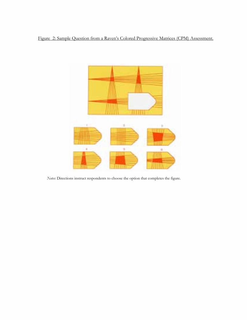
Figure 2: Sample Question from a Raven’s Colored Progressive Matrices (CPM) Assessment.
Notes: Directions instruct respondents to choose the option that completes the figure.
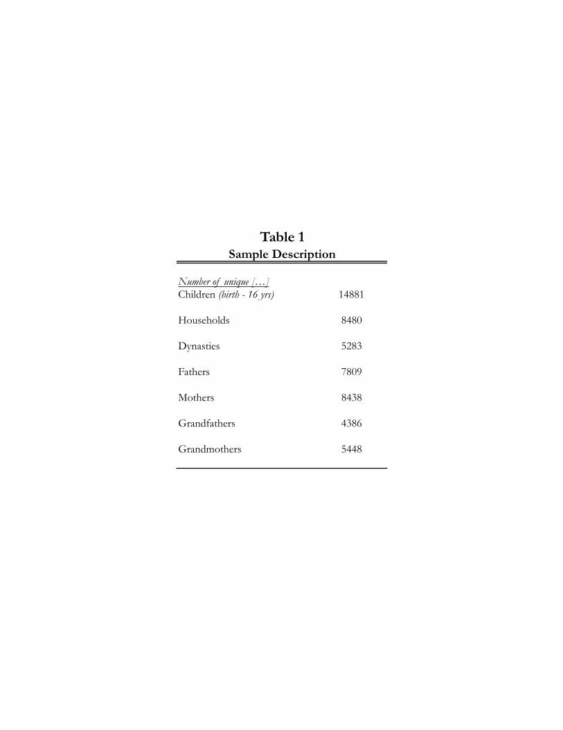
Number of unique […]Children (birth - 16 yrs) 14881
Households 8480
Dynasties 5283
Fathers 7809
Mothers 8438
Grandfathers 4386
Grandmothers 5448
Table 1Sample Description

All Children (Birth - 16 yrs)
Height-for-Age (Birth - 6 yrs)
Attended Kindergarten (6 - 14 yrs)
Cognitive Score (7 - 16 yrs)
OutcomesHeight-for-Age (z-score) -1.14
(0.02)Attended Kindergarten (%) 50.8
(0.58)Cognitive Score (%) 69.6
(0.21)Liquid Assets of […]*Household 1928.8 1949.1 1854.7 1902.7
(38.9) (60.3) (49.7) (51.5)Dynasty 2579.5 3027.9 2355.9 2148.9
(47.3) (74.6) (64.7) (59.5)Father 872.2 821.5 907.9 904.2
(22.9) (37.1) (29.9) (28.2)Mother 762.8 680.6 822.4 831.3
(17.7) (22.1) (26.8) (27.1)Grandfather 799.8 885.6 658.3 657.9
(35.3) (51.5) (37.7) (42.2)Grandmother 616.7 697.4 510.8 480.5
(19.9) (29.4) (22.7) (23.7)Additional ControlsAge 7.37 2.88 9.79 11.26
(0.04) (0.02) (0.03) (0.03)Female 0.48 0.48 0.48 0.49
(0.00) (0.01) (0.01) (0.01)
Co-reside with Father 0.81 0.87 0.78 0.76(0.00) (0.00) (0.00) (0.00)
Co-reside with Mother 0.90 0.96 0.87 0.85(0.00) (0.00) (0.00) (0.00)
Household Size 4.98 4.86 5.06 5.08(0.02) (0.02) (0.02) (0.02)
Dynasty Size 11.16 11.94 10.86 10.45(0.05) (0.08) (0.07) (0.07)
Age of […]Father 38.7 34.4 41.0 42.5
(0.08) (0.09) (0.10) (0.10)Mother 34.1 29.8 36.4 37.9
(0.07) (0.08) (0.08) (0.08)Grandfather 62.0 59.9 64.7 65.5
(0.13) (0.16) (0.19) (0.21)Grandmother 58.5 55.9 61.2 62.1
(0.11) (0.14) (0.16) (0.17)Years of Education of […]Father 8.52 9.15 8.22 7.96
(0.04) (0.05) (0.05) (0.05)Mother 8.03 8.96 7.56 7.26
(0.03) (0.05) (0.05) (0.05)Grandfather 4.89 5.47 4.54 4.33
(0.03) (0.05) (0.04) (0.04)Grandmother 3.71 4.30 3.38 3.16
(0.03) (0.04) (0.04) (0.04)
Maternal Height (cm) 162.0 162.6 162.0 161.6(0.05) (0.07) (0.06) (0.06)
Paternal Height (cm) 151.1 151.5 151.0 150.9(0.04) (0.06) (0.06) (0.06)
Urban Household 0.51 0.53 0.50 0.49(0.00) (0.01) (0.01) (0.01)
N. Observations 14881 6567 7493 7727* In Rp0,000 (~ 1 USD)
Table 2Descriptive Statistics
Sample

Child OutcomesHeight-for-Age Attended Kindergarten (%) Cognitive Score (%)
Household Assets 0.06** 4.25*** 0.80**(0.03) (0.97) (0.41)
Dynasty Fixed Effects Yes Yes Yes
N. Observations 6567 7493 7727
*** Significant at the 1% level, ** Significant at the 5% level.
Table 3Household Unitary Tests
Notes: All regressions include dynasty fixed effects and assets in log form, as well as controls for gender, age, household size and composition,parental education, age and gender of the household head and location as described in the text. Standard errors in parentheses account forclustering at the family level.

Panel A: Estimates for Tests of the Collective Model
Child OutcomesHeight-for-Age Attended Kindergarten (%) Cognitive Score (%)
Household Assets 0.09*** 5.02*** 1.17***(0.02) (0.45) (0.18)
Dynasty Assets 0.03** 1.93*** 0.45**(0.02) (0.52) (0.22)
N. Observations 6567 7493 7727Panel BUnitary Testsp-value 0.02 0.00003 0.02
Ratios of Coefficients2.65* 2.60*** 2.60*(1.41) (0.78) (1.40)
Panel C: Collective Model Nonlinear Wald Tests (p-values)
Test of equality of ratios between […] and […] p-valueHeight-for-Age Attend Kindergarten 0.97Height-for-Age Cognitive Score 0.98
Attend Kindergarten Cognitive Score 0.99
All Ratios 0.99
Table 4Household Pareto Efficiency Tests
Household to Dynasty Assets
Notes: Panel A: All regressions include assets in log form, as well as controls for gender, age, household and dynasty size and composition,parental education, age and gender of the household and dynasty head and location as described in the text. Standard errors in parenthesisaccount for clustering at the family level. Panel B: The p-values correspond to a test of the unitary mode based on the equivalence of thehousehold and dynasty asset effects, where the null is that the two coefficients for each outcome in Panel A are equal. The collective modeltest relies on the equivalence of the ratio of coefficients from Panel A. The ratios and their standard errors are calculated using the deltamethod, allowing for clustering at the family level. Panel C: The p-values correspond to results from nonlinear Wald tests where the null isPareto efficiency. These tests compare the equivalence of the ratios shown in Panel B for the outcome pairs in each row. The final p -value is for the test of equivalence across all three ratios. *** Significant at the 1% level, ** Significant at the 5% level, * Significant at the 10% level.

Child OutcomesHeight-for-Age Attended Kindergarten (%) Cognitive Score (%)
Father's Assets 0.02 1.72*** 0.25(0.02) (0.51) (0.19)
Mother's Assets 0.05*** 2.32*** 0.66***(0.02) (0.53) (0.19)
Grandfather's Assets 0.01 -0.46 0.13(0.02) (0.78) (0.31)
Grandmother's Assets 0.01 1.48** 0.12(0.02) (0.72) (0.31)
Rest of Household Assets 0.04** 1.21*** 0.35**(0.02) (0.45) (0.16)
Rest of Dynasty Assets 0.03*** 1.46*** 0.24(0.01) (0.36) (0.15)
N. Observations 6567 7493 7727
*** Significant at the 1% level, ** Significant at the 5% level, * Significant at the 10% level
Table 5Individual Level Regressions for Tests of the Collective Model
Notes: Each regression includes assets at the individual level in quartic root form, and controls for the age and gender of the child, householdand dynasty size and composition, age and education of parents and grandparents, and location as described in the text. Ratios and theirstandard errors similar to those shown in Panel B of Table 4 are not reported for space concerns, but are available from the authors uponrequest. Standard errors in parentheses account for clustering at the family level.
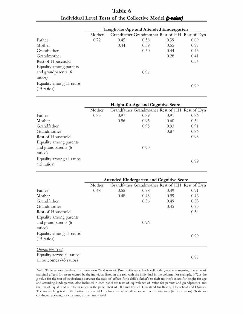
Mother Grandfather Grandmother Rest of HH Rest of DynFather 0.72 0.45 0.58 0.39 0.69Mother 0.44 0.39 0.55 0.97Grandfather 0.50 0.44 0.43Grandmother 0.28 0.41Rest of Household 0.54Equality among parents and grandparents (6 ratios)
0.97
Equality among all ratios (15 ratios)
0.99
Mother Grandfather Grandmother Rest of HH Rest of DynFather 0.83 0.97 0.89 0.91 0.86Mother 0.96 0.95 0.60 0.54Grandfather 0.95 0.93 0.91Grandmother 0.87 0.86Rest of Household 0.93Equality among parents and grandparents (6 ratios)
0.99
Equality among all ratios (15 ratios)
0.99
Mother Grandfather Grandmother Rest of HH Rest of DynFather 0.48 0.55 0.78 0.49 0.91Mother 0.48 0.43 0.99 0.46Grandfather 0.56 0.49 0.53Grandmother 0.45 0.73Rest of Household 0.54Equality among parents and grandparents (6 ratios)
0.96
Equality among all ratios (15 ratios)
0.99
Overarching TestEquality across all ratios, all outcomes (45 ratios)
0.97
Notes: Table reports p-values from nonlinear Wald tests of Pareto efficiency. Each cell is the p-value comparing the ratio ofmarginal effects for assets owned by the individual listed in the row with the individual in the column. For example, 0.72 is thep-value for the test of equivalence between the ratio of effects for a child's father's to their mother's assets for height-for-ageand attending kindergarten. Also included in each panel are tests of equivalence of ratios for parents and grandparents, andthe test of equality of all fifteen ratios in the panel. Rest of HH and Rest of Dyn stand for Rest of Household and Dynasty.The overarching test at the bottom of the table is for equality of all ratios across all outcomes (45 total ratios). Tests areconducted allowing for clustering at the family level.
Table 6Individual Level Tests of the Collective Model (p-values)
Height-for-Age and Attended Kindergarten
Height-for-Age and Cognitive Score
Attended Kindergarten and Cognitive Score

Child OutcomesHeight-for-Age Attended Kindergarten (%) Cognitive Score (%)
Household Per Capita 0.12** 5.47*** 1.86**Expenditure (0.06) (1.92) (0.88)
Dynasty Fixed Effects Yes Yes Yes
N. Observations 6567 7493 7727
Table A.1Household Unitary Tests - Monthly Per Capita Expenditure
Notes: All regressions include dynasty fixed effects and household per capita expenditure in log form, as well as controls for gender, age, household size and composition, parental education, age and gender of the household head and location as described in the text. Standard errors in parentheses account for clustering at the family level.
*** Significant at the 1% level, ** Significant at the 5% level.

Panel A: Estimates for Tests of the Collective Model
Child OutcomesHeight-for-Age Attended Kindergarten (%) Cognitive Score (%)
Household Per Capita 0.17*** 9.28*** 2.46***Expenditure (0.03) (1.07) (0.36)
Dynasty Per Capita 0.08** 1.60 0.48Expenditure (0.03) (1.05) (0.41)
N. Observations 6567 7493 7727Panel BUnitary Testsp-value 0.08 0.00002 0.0008
Ratios of Coefficients2.05** 5.80 5.16(0.95) (3.93) (4.60)
Panel C: Collective Model Nonlinear Wald Tests (p-values)
Test of equality of ratios between […] and […] p-valuesHeight-for-Age Attended Kindergarten 0.18Height-for-Age Cognitive Score 0.28
Attended Kindergarten Cognitive Score 0.92
All Ratios 0.60
Table A.2Household Pareto Efficiency Tests - Monthly Per Capita Expenditure
Household to Dynasty PCE
Notes: Panel A: All regressions include monthly per-capita expenditure in log form, as well as controls for gender, age, household anddynasty size and composition, parental education, age and gender of the household and dynasty head and location as described in the text.Standard errors in parenthesis account for clustering at the family level. Panel B: The p-values correspond to a test of the unitary modebased on the equivalence of the household and dynasty effects, where the null is that the two coefficients in Panel A are equal. Thecollective model test relies on the equivalence of the ratio of coefficients from Panel A. The ratios and their standard errors are calculatedusing the delta method allowing for clustering at the family level. Panel C: The p-values correspond to results from nonlinear Wald testswhere the null is Pareto efficiency. These tests compare the equivalence of the ratios shown in Panel B for the outcome pairs in each row.The final p-value is for the test of equivalence across all three ratios.*** Significant at the 1% level, ** Significant at the 5% level.