exponential time - arxiv.org e-print archive connectivity problems parameterized by treewidth in...
TRANSCRIPT
Solving connectivity problems parameterized by treewidth in singleexponential time
Marek Cygan∗ Jesper Nederlof† Marcin Pilipczuk‡ Michał Pilipczuk§
Johan van Rooij¶ Jakub Onufry Wojtaszczyk‖
Abstract
For the vast majority of local graph problems standard dynamic programming techniques give ctw|V |O(1) algo-rithms, where tw is the treewidth of the input graph. On the other hand, for problems with a global requirement (usu-ally connectivity) the best–known algorithms were naive dynamic programming schemes running in twO(tw)|V |O(1)
time.We breach this gap by introducing a technique we dubbed Cut&Count that allows to produce ctw|V |O(1) Monte
Carlo algorithms for most connectivity-type problems, including HAMILTONIAN PATH, FEEDBACK VERTEX SET
and CONNECTED DOMINATING SET, consequently answering the question raised by Lokshtanov, Marx and Saurabh[SODA’11] in a surprising way. We also show that (under reasonable complexity assumptions) the gap cannot bebreached for some problems for which Cut&Count does not work, like CYCLE PACKING.
The constant c we obtain is in all cases small (at most 4 for undirected problems and at most 6 for directed ones),and in several cases we are able to show that improving those constants would cause the Strong Exponential TimeHypothesis to fail.
Our results have numerous consequences in various fields, like FPT algorithms, exact and approximate algorithmson planar and H-minor-free graphs and algorithms on graphs of bounded degree. In all these fields we are able toimprove the best-known results for some problems.
1 Introduction and notationThe notion of treewidth, introduced in 1984 by Robertson and Seymour [56], has in many cases proved to be agood measure of the intrinsic difficulty of various NP-hard problems on graphs, and a useful tool for attacking thoseproblems. Many of them can be efficiently solved through dynamic programming if we assume the input graph tohave bounded treewidth. For example, an expository algorithm to solve VERTEX COVER and INDEPENDENT SETrunning in time 4tw(G)|V |O(1) is described in the algorithms textbook by Kleinberg and Tardos [43], while the bookof Niedermeier [52] on fixed-parameter algorithms presents an algorithm with running time 2tw(G)|V |O(1).
The interest in algorithms for graphs of bounded treewidth stems from their utility: such algorithms are used assub-routines in a variety of settings. Amongst them prominent are approximation algorithms [19, 29] and parametrizedalgorithms [22] for a vast number of problems on planar, bounded-genus andH-minor-free graphs, including VERTEXCOVER, DOMINATING SET and INDEPENDENT SET; there are applications for parametrized algorithms in generalgraphs [50, 60] for problems like CONNECTED VERTEX COVER and CUTWIDTH; and exact algorithms [30, 63] suchas MINIMUM MAXIMAL MATCHING and DOMINATING SET.
In many cases, where the problem to be solved is “local” (loosely speaking this means that the property of theobject to be found can be verified by checking separately the neighbourhood of each vertex) matching upper and∗Institute of Informatics, University of Warsaw, Poland, [email protected]†Department of Informatics, University of Bergen, Norway, [email protected]‡Institute of Informatics, University of Warsaw, Poland, [email protected]§Faculty of Mathematics, Informatics and Mechanics, University of Warsaw, Poland, [email protected]¶Department of Information and Computing Sciences, Utrecht University, The Netherlands, [email protected]‖Google Inc., Cracow, Poland, [email protected]
1
arX
iv:1
103.
0534
v1 [
cs.D
S] 2
Mar
201
1
lower bounds for the runtime of the optimal solution are known. For instance for the aforementioned 2tw(G)|V |O(1)
algorithm for VERTEX COVER there is a matching lower bound — unless the Strong Exponential Time Hypothesisfails, there is no algorithm for VERTEX COVER running quicker than (2− ε)tw(G) for any ε > 0.
On the other hand, when the problem involves some sort of a “global” constraint — e.g., connectivity — the bestknown algorithms usually have a runtime on the order of tw(G)O(tw(G))|V |O(1). In these cases the typical dynamicprogram has to keep track of all the ways in which the solution can traverse the corresponding separator of the treedecomposition, that is Ω(ll) on the size l of the separator, and therefore of treewidth. This obviously implies weakerresults in the applications mentioned above. This problem was observed, for instance, by F. Dorn, F. Fomin and D.Thilikos [22, 23] and by H. Bodlaender et al. in [24]. The question whether the known 2O(tw(G) log tw(G))|V |O(1)
parametrized algorithms for HAMILTONIAN PATH, CONNECTED VERTEX COVER and CONNECTED DOMINATINGSET are optimal was asked by D. Lokshtanov, D. Marx and S. Saurabh [48].
To explain why the 2O(tw(G) log tw(G)) dynamic programming algorithms for connectivity problems were thoughtto be optimal we recall the concept of a Myhill-Nerode style equivalence class. In this case two partial solutions of asubtree of the tree decomposition are said to be equivalent if they are consistent with the same set of partial solutionson the remainder of the tree decomposition [37]. The states of the naive dynamic program reflect Myhill-Nerode styleequivalence classes, and it seemed to be necessary for any algorithm to memoize the information about each class, asit could be needed during further computation (see for example the recent work by Lokshtanov et al. [47, 48]). Fromthis point of view the results of this paper come as a significant surprise.
1.1 Our resultsIn this paper we introduce a technique we dubbed “Cut&Count” that allows us to deal with connectivity-type problemsthrough randomization. For most problems involving a global constraint our technique gives a randomized algorithmwith runtime ctw(G)|V |O(1). In particular we are able to give such algorithms for the three problems mentioned in[48], as well as for all the other sample problems mentioned in [23]: LONGEST PATH, LONGEST CYCLE, FEEDBACKVERTEX SET, HAMILTONIAN CYCLE and GRAPH METRIC TRAVELLING SALESMAN PROBLEM. Moreover, boththe constant c and the exponent in |V |O(1) is in all cases well defined and small.
The randomization we mention comes from the usage of the Isolation Lemma [51]. This gives us Monte Carloalgorithms with a one-sided error. The formal statement of a typical result is as follows:
Theorem 1.1. There exists a randomized algorithm, which given a graph G with n vertices, a tree decomposition ofG of width t and a number k in 3tnO(1) time either states that there exists a connected vertex cover of size at most kin G, or that it could not verify this hypothesis. If there indeed exists such a cover, the algorithm will return “unableto verify” with probability at most 1/2.
We shall denote such an algorithm, which either confirms the existence of the object we are asking about or returns“unable to verify”, and returns “unable to verify” with probability no larger than 1/2 if the answer is positive, analgorithm with false negatives.
We see similar results for a plethora of other global problems. As the exact value of c in the ctw(G) expression isoften important, we gather here the results we obtain:
Theorem 1.2. There exist Monte-Carlo algorithms that given a tree decomposition of the (underlying undirectedgraph of the) input graph of width t solve the following problems:
1. STEINER TREE in 3t|V |O(1) time.
2. FEEDBACK VERTEX SET in 3t|V |O(1) time.
3. CONNECTED VERTEX COVER in 3t|V |O(1) time.
4. CONNECTED DOMINATING SET in 4t|V |O(1) time.
5. CONNECTED FEEDBACK VERTEX SET in 4t|V |O(1) time.
6. CONNECTED ODD CYCLE TRANSVERSAL in 4t|V |O(1) time.
2

7. MIN CYCLE COVER in 6t|V |O(1) time for directed graphs and in 4t|V |O(1) time for undirected graphs.
8. Directed LONGEST PATH in 6t|V |O(1) time and undirected LONGEST PATH in 4t|V |O(1) time. This, in partic-ular, gives the same times for solving HAMILTONIAN PATH for the directed and undirected cases, respectively.
9. Directed LONGEST CYCLE in 6t|V |O(1) time and undirected LONGEST CYCLE in 4t|V |O(1) time. This, inparticular, gives the same times for solving HAMILTONIAN CYCLE for the directed and undirected cases, re-specitvely.
10. EXACT k-LEAF SPANNING TREE and, in particular, MINIMUM LEAF TREE and MAXIMUM LEAF TREE in4t|V |O(1) time for undirected graphs.
11. EXACT k-LEAF OUTBRANCHING and, in particular MINIMUM LEAF OUTBRANCHING and MAXIMUM LEAFOUTBRANCHING in 6t|V |O(1) time for directed graphs.
12. MAXIMUM FULL DEGREE SPANNING TREE in 4t|V |O(1) time.
13. GRAPH METRIC TRAVELLING SALESMAN PROBLEM in 4t|V |O(1) time for undirected graphs.
The algorithms cannot give false positives and may give false negatives with probability at most 1/2.
For a number of these results we have matching lower bounds, such as the following one:
Theorem 1.3. Unless the Strong Exponential Time Hypothesis is false, there do not exist a constant ε > 0 and analgorithm that given an instance (G = (V,E), T, k) together with a path decomposition of the graph G of width psolves the STEINER TREE problem in (3− ε)p|V |O(1) time.
We have such matching lower bounds for the following problems: CONNECTED VERTEX COVER, CONNECTEDDOMINATING SET, CONNECTED FEEDBACK VERTEX SET, CONNECTED ODD CYCLE TRANSVERSAL, FEEDBACKVERTEX SET, STEINER TREE and EXACT k-LEAF SPANNING TREE. We feel that the first four results are of particularinterest here and should be compared to the algorithms and lower bounds for the analogous problems without theconnectivity requirement. For instance in the case of CONNECTED VERTEX COVER the results show that the increasein running time to 3tw(G)nO(1) from the 2tw(G)nO(1) algorithm of [52] for VERTEX COVER is not an artifact ofthe Cut&Count technique, but rather an intrinsic characteristic of the problem. We see a similar increase of the baseconstant by one for the other three mentioned problems.
We have found Cut&Count to fail for two maximization problems: CYCLE PACKING and MAX CYCLE COVER.We believe this is an example of a more general phenomenon — problems that ask to maximize (instead of minimizing)the number of connected components in the solution seem more difficult to solve than the problems of minimization(including problems where we demand that the solution forms a single connected component). As evidence we presentlower bounds for the time complexity of solutions to such problems, proving that ctw(G) solutions of these problemsare unlikely:
Theorem 1.4. Unless the Exponential Time Hypothesis is false, there does not exist a 2o(p log p)|V |O(1) algorithm forsolving CYCLE PACKING or MAX CYCLE COVER. The parameter p denotes the width of a given path decompositionof the input graph.
To further verify this intuition, we investigated an artificial problem (the MAXIMALLY DISCONNECTED DOMI-NATING SET), in which we ask for a dominating set with the largest possible number of connected components, andindeed we found a similar phenomenon:
Theorem 1.5. Unless the Exponential Time Hypothesis is false, there does not exist a 2o(p log p)|V |O(1) algorithmfor solving MAXIMALLY DISCONNECTED DOMINATING SET. The parameter p denotes the width of a given pathdecomposition of the input graph.
A reader interested in just the basic workings of the Cut&Count technique will likely find the descriptions and theintuition needed in the first three sections of this work. The rest of the rather formidable volume is devoted to refinedapplications, in some cases needed to obtained the optimal constants, as well as arguments showing the aforementionedoptimality, and can — in a sense — be considered “advanced material”.
3

1.2 Previous workThe Cut&Count technique has two main ingredients. The first is an algebraic approach, where we assure that objectswe are not interested in are counted an even number of times, and then do the calculations in Z2 or in a field ofcharacteristic 2, which causes them to disappear. This line of reasoning goes back to Tutte [61], and was recently usedby Bjorklund [6] and Bjorklund et. al [9].
The second is the idea of defining the connectivity requirement through cuts, which is frequently used in approx-imation algorithms via linear programming relaxations. In particular cut based constraints were used in the Held andKarp relaxation for the TRAVELLING SALESMAN PROBLEM problem from 1970 [34, 35] and appear up to now in thebest known approximation algorithms, for example in the recent algorithm for the STEINER TREE problem by Byrkaet al. [13]. To the best of our knowledge the idea of defining problems through cuts was never used in the exact andparameterized settings.
A number of papers circumvent the problems stemming from the lack of singly exponential algorithms parametrizedby treewidth for connectivity–type problems. For instance in the case of parametrized algorithms, sphere cuts [22,24] (for planar and bounded genus graphs) and Catalan structures [23] (for H-minor-free graphs) were used toobtain 2O(
√k)|V |O(1) algorithms for a number of problems with connectivity requirements. To the best of our
knowledge, however, no attempt to attack the problem directly was published before; indeed the non-existence of2o(tw(G) log tw(G)) algorithms was deemed to be more likely.
1.3 Consequences of the Cut&Count techniqueAs alredy mentioned, algorithms for graphs with a bounded treewidth have a number of applications in variousbranches of algorithmics. Thus, it is not a surprise that the results obtained by our technique give a large numberof corollaries. To keep the volume of this paper manageable, we do not explore all possible applications, but only givesample applications in various directions.
We would like to emphasize that the strength of the Cut&Count technique shows not only in the quality of theresults obtained in various fields, which are frequently better than the previously best known ones, achieved through aplethora of techniques and approaches, but also in the ease in which new strong results can be obtained.
1.3.1 Consequences for FPT algorithms
Let us recall the definition of the FEEDBACK VERTEX SET problem:
FEEDBACK VERTEX SET Parameter: kInput: An undirected graph G and an integer kQuestion: Is it possible to remove k vertices from G so that the remaining vertices induce a forest?
This problem is on Karp’s original list of 21 NP-complete problems [42]. It has also been extensively studied fromthe parametrized complexity point of view. Let us recall that in the fixed-parameter setting (FPT) the problem comeswith a parameter k, and we are looking for a solution with time complexity f(k)nO(1), where n is the input size andf is some function (usually exponential in k). Thus, we seek to move the intractability of the problem from the inputsize to the parameter.
There is a long sequence of FPT algorithms for FEEDBACK VERTEX SET [4, 10, 16, 18, 26, 27, 33, 41, 53, 54].The best — so far — result in this series is the 3.83kkn2 result of Cao, Chen and Liu [14]. Our technique gives animprovement of their result:
Theorem 1.6. There exists a Monte-Carlo algorithm solving the FEEDBACK VERTEX SET problem in a graph with nvertices in 3knO(1) time and polynomial space. The algorithm cannot give false positives and may give false negativeswith probability at most 1/2.
We give similar improvements for CONNECTED VERTEX COVER (from the 2.4882knO(1) of [5] to 2knO(1)) andCONNECTED FEEDBACK VERTEX SET (from the 46.2knO(1) of [49] to 3knO(1)).
4

1.3.2 Parametrized algorithms for H-minor-free graphs
A large branch of applications of algorithms parametrized with treewidth is the bidimensionality theory, used to findsubexponential algorithms for various problems in H-minor-free graphs. In this theory we use the celebrated minortheorem of Robertson and Seymour [57], which ensures that any H-minor-free graph either has treewidth boundedby C
√k, or a 2
√k × 2
√k lattice as a minor. In the latter case we are assumed to be able to answer the problem in
question (for instance a 2√k × 2
√k lattice as a minor guarantees that the graph does not have a VERTEX COVER or
CONNECTED VERTEX COVER smaller than k). Thus, we are left with solving the problem with the assumption ofbounded treewidth. In the case of, for instance, VERTEX COVER a standard dynamic algorithm suffices, thus giving usa 2O(
√k) algorithm to check whether a graph has a vertex cover no larger than k. In the case of CONNECTED VERTEX
COVER, however, the standard dynamic algorithm gives a 2O(√k log k) complexity — thus, we lose a logarithmic factor
in the exponent.There were a number of attempts to deal with this problem, taking into account the structure of the graph, and
using it to deduce some properties of the tree decomposition under consideration. The latest and most efficient ofthose approaches is due to Dorn, Fomin and Thilikos [23], and exploits the so called Catalan structures. The approachdeals with most of the problems mentioned in our paper, and is probably applicable to the remaining ones. Thus, thegain here is not in improving the running times (though our approach does improve the constants hidden in the big-Onotation these are rarely considered to be important in the bidimensionality theory), but rather in simplifying the proof— instead of delving into the combinatorial structure of each particular problem, we are back to a simple frameworkof applying the Robertson-Seymour theorem and then following up with a dynamic program on the obtained treedecomposition.
The situation is more complicated in the case of problems on directed graphs. A full equivalent of the bidimension-ality theory is not developed for such problems, and only a few problems have subexponential parametrized algorithmsavailable [2, 21]. One of the approaches is to mimic the bidimensionality approach, which again leads to solving aproblem on a graph of bounded treewidth — such an approach is taken by Dorn et al. in [21] for MAXIMUM LEAF
OUTBRANCHING to obtain a 2O(√k log k) algorithm. In this case, a straightforward substitution of our 6tw(G)|V |O(1)
algorithm for the dynamic algorithm used by Dorn et al. will give the following improvement:
Theorem 1.7. There exists a Monte-Carlo algorithm solving the k-MAXIMUM LEAF OUTBRANCHING problem in2O(√k)|V |O(1) time for directed graphs for which the underlying undirected graph excludes a fixed graph H as a
minor. The algorithm cannot give false positives and may give false negatives with probability at most 1/2.
1.3.3 Consequences for Exact Algorithms for graphs of bounded degree
Another application of our methods can be found in the field of solving problems with a global constraint in graphsof bounded degree. The problems that have been studied in this setting are mostly local in nature (such as VERTEXCOVER, see, e.g., [12]); however global problems such as the TRAVELLING SALESMAN PROBLEM and HAMILTO-NIAN CYCLE have also received considerable attention [8, 28, 32, 39].
Here the starting point is the following theorem by Fomin et al. [30]:
Theorem 1.8 (Fomin, Gaspers, Saurabh, Stepanov). For any ε > 0 there exists an integer nε such that for any graphG with n > nε vertices,
pw(G) ≤ 1
6n3 +
1
3n4 +
13
30n5 + n≥6 + εn,
where ni is the number of vertices of degree i in G for any i ∈ 3, . . . , 5 and n≥6 is the number of vertices of degreeat least 6.
This theorem is constructive, and the corresponding path decompostion (and, consequently, tree decomposition)can be found in polynomial time.
Combining this theorem with our results gives algorithms running in faster than 2n for graphs of maximum degree3, 4 and (in the case of the 3tw(G) and 4tw(G) algorithms) 5, as follows:
Corollary 1.9. There exist randomized algorithms that solve the following problems:
5
• STEINER TREE, FEEDBACK VERTEX SET and CONNECTED VERTEX COVER in O(1.201n) time for cubicgraphs, O(1.443n) time for graphs of maximum degree 4 and O(1.61n) time for graphs of maximum degree 5;
• CONNECTED DOMINATING SET, CONNECTED ODD CYCLE TRANSVERSAL, CONNECTED FEEDBACK VER-TEX SET, EXACT k-LEAF SPANNING TREE, MAXIMUM FULL DEGREE SPANNING TREE and GRAPH MET-RIC TRAVELLING SALESMAN PROBLEM as well as undirected versions of MIN CYCLE COVER, LONGESTPATH and LONGEST CYCLE in O(1.26n) time for cubic graphs, O(1.588n) for graphs of maximum degree 4and O(1.824n) for graphs of maximum degree 5;
• Directed versions of MIN CYCLE COVER, LONGEST PATH and LONGEST CYCLE, as well as for EXACT k-LEAF OUTBRANCHING, in O(1.349n) for cubic graphs and in O(1.818n) for graphs of maximum degree 4.
All the aforementioned algorithms are Monte Carlo algorithms with false negatives.
The TRAVELLING SALESMAN PROBLEM in its full generality does not fall under the Cut&Count regime; howeverfor graphs of degree four theO(1.588n) algorithm obtained for GRAPH METRIC TRAVELLING SALESMAN PROBLEM(which can easily be extended to the case of the TRAVELLING SALESMAN PROBLEM with polynomially boundedweights) is significantly faster than the best known algorithm for the case of unbounded weights of Gebauer [32],which runs in 1.733n time. For the case of degree 5 (where we give an O(1.824n) algorithm for the TRAVELLINGSALESMAN PROBLEM with polynomially bounded weights) the best known result in the general weight case is the(2 − ε)n algorithm of Bjorklund et al. [8]. It is worth noticing that in the case of cubic graphs we automaticallyobtain an algorithm for GRAPH METRIC TRAVELLING SALESMAN PROBLEM running in 2n/3+εnnO(1) time, whichcoincides with the time complexity of the algorithm for TRAVELLING SALESMAN PROBLEM of Eppstein [28]. Thecurrently fastest algorithm for TRAVELLING SALESMAN PROBLEM in cubic graphs is due to Iwama and Nakashima[39].
1.3.4 Consequences for exact algorithms on planar graphs
Here we begin with a consequence of the work of Fomin and Thilikos [31]:
Proposition 1.10. For any planar graph G, tw(G) + 1 ≤ 32
√4.5n ≤ 3.183
√n. Moreover a tree decomposition of
such width can be found in polynomial time.
Using this we immediately obtain c√n algorithms for solving problems with a global constraint on planar graphs
with good constants. For instance for the HAMILTONIAN CYCLE problem on planar graphs we obtain the followingresult:
Corollary 1.11. There exists a randomized algorithm with false negatives solving HAMILTONIAN CYCLE on planargraphs in O(43.183
√n) = O(26.366
√n) time.
To the best of our knowledge the best algorithm known so far was the O(26.903√n) of Bodlaender et al. [24].
Similarly, we obtain anO(26.366√n) algorithm for LONGEST CYCLE on planar graphs (compare to theO(27.223
√n)
of [24]), and — as in the previous subsections — well-behaved c√n algorithms for all mentioned problems.
1.4 Organization of the paperIn the introduction we present the contents of the paper. Subsection 1.1 states the main results obtained by us. Afteranalyzing the connections to previous works in Subsection 1.2 we turn to giving sample consequences in Subsection1.3. We finish the introduction by giving this outline.
Section 2 is devoted to presenting the background material for our algorithms. In particular in Subsection 2.2 werecall the notion of treewidth and dynamic programming on tree decompositions, while in Subsection 2.3 we introducethe Isolation Lemma.
In Section 3 we present the Cut&Count technique on two examples: the STEINER TREE problem and the DI-RECTED MIN CYCLE COVER problem. We go into all the details, as we aim to present not only the algorithms and
6
proofs, but also the intuition behind them. We use those intuitions in Section 4, where we give sketches of algorithmsfor all the other problems mentioned in Theorem 1.2.
In Section 5 we move to lower bounds. In Subsection 5.1 we present evidence that problems in which we maximizethe number of connected components are unlikely to have ctw(G)|V |O(1) algorithms. In Subsection 5.2 we providearguments that several of the algorithms provided in Section 3 have time complexity which is hard to improve. Wefinish the paper with a number of conclusions and open problems in Section 6
As the reader might have already noticed, there is a quite a large amount of material covered in this paper. To keepit readable a considerable number of proofs and analyses was postponed to the appendix. Thus, in Appendix A we givedetailed descriptions of all the algorithms sketched in Section 4. In particular in Part A.1 we describe all the variantsof the Fast Subset Convolution technique we use to decrease the constants in our algorithms. Appendix B is devoted tothe proofs of the results announced in Subsection 1.3.1 — Theorem 1.6 and its analogues for CONNECTED VERTEXCOVER and CONNECTED FEEDBACK VERTEX SET. In Appendix C we turn to the proofs of the lower bounds statedin Subsection 5.1, while Appendix D gives proofs for tight lower bounds stated in Subsection 5.2.
2 Preliminaries and notation
2.1 NotationLet G = (V,E) be a graph (possibly directed). By V (G) and E(G) we denote the sets of vertices and edges of G,respectively. For a vertex set X ⊆ V (G) by G[X] we denote the subgraph induced by X . For an edge set X ⊆ E, wetake V (X) to denote the set of the endpoints of the edges of X , and by G[X] — the subgraph (V,X). Note that in thegraph G[X] for an edge set X the set of vertices remains the same as in the graph G.
For an undirected graph G = (V,E), the open neighbourhood of a vertex v, denoted N(v), stands for u ∈ V :uv ∈ E, while the closed neighbourhood N [v] is N(v) ∪ v. Similarly, for a set X ⊆ V (G) by N [X] we mean⋃v∈X N [v] and by N(x) we mean N [X] \X .
By a cut of a set X ⊆ V we mean a pair (X1, X2), with X1 ∩X2 = ∅, X1 ∪X2 = X . We refer to X1 and X2 asto the (left and right) sides of the cut.
We denote the degree of a vertex v by deg(v). degH(v) denotes the degree of v in the subgraph H . For X ⊆ Vor X ⊆ E, degX(v) is a short for degG[X](v). If G is a directed graph and X ⊆ V or X ⊆ E, we denote the in- andout-degree of v in G[X] by indegG[X](v) and outdegG[X](v) respectively.
For an edge e = uv by subdividing it s times (for s > 0) we mean the following operation: (1) remove the edge e,(2) add s vertices xe,1, . . . , xe,s, (3) add edges uxe,1, xe,1xe,2, . . . , xe,k−1xe,s, xe,sv.
In a directed graph G by weakly connected components we mean the connected components of the underlyingundirected graph. For a (directed) graph G, we let cc(G) denote the number of (weakly) connected components of G.
For two bags x, y of a rooted tree we say that y is a descendant of x if it is possible to reach x when starting at yand going only up the tree. In particular x is its own descendant.
We denote the symmetric difference of two sets A and B by A4B. For two integers a, b we use a ≡ b to indicatethat a is even if and only if b is even. We use Iverson’s bracket notation: if p is a predicate we let [p] be 1 if p if trueand 0 otherwise. If ω : U → 1, . . . , N, we shorthand ω(S) =
∑e∈S ω(e) for S ⊆ U .
For a function s by s[v → α] we denote the function s \ (v, s(v)) ∪ (v, α). Note that this definition worksregardless of whether s(v) is already defined or not.
2.2 Treewidth and pathwidth2.2.1 Tree Decompositions
Definition 2.1 (Tree Decomposition, [56]). A tree decomposition of a (undirected or directed) graph G is a tree T inwhich each vertex x ∈ T has an assigned set of vertices Bx ⊆ V (called a bag) such that
⋃x∈TBx = V with the
following properties:
• for any uv ∈ E, there exists an x ∈ T such that u, v ∈ Bx.
7

• if v ∈ Bx and v ∈ By , then v ∈ Bz for all z on the path from x to y in T.
The treewidth tw(T) of a tree decomposition T is the size of the largest bag of T minus one, and the treewidth ofa graph G is the minimum treewidth over all possible tree decompositions of G.
Dynamic programming algorithms on tree decompositions are often presented on nice tree decompositions whichwere introduced by Kloks [44]. We refer to the tree decomposition definition given by Kloks as to a standard nice treedecomposition.
Definition 2.2. A standard nice tree decomposition is a tree decomposition where:
• every bag has at most two children,
• if a bag x has two children l, r, then Bx = Bl = Br,
• if a bag x has one child y, then either |Bx| = |By|+ 1 and By ⊆ Bx or |Bx|+ 1 = |By| and Bx ⊆ By .
We present a slightly different definition of a nice tree decomposition.
Definition 2.3 (Nice Tree Decomposition). A nice tree decomposition is a tree decomposition with one special bag zcalled the root with Bz = ∅ and in which each bag is one of the following types:
• Leaf bag: a leaf x of T with Bx = ∅.
• Introduce vertex bag: an internal vertex x of T with one child vertex y for which Bx = By ∪ v for somev /∈ By . This bag is said to introduce v.
• Introduce edge bag: an internal vertex x of T labeled with an edge uv ∈ E with one child bag y for whichu, v ∈ Bx = By . This bag is said to introduce uv.
• Forget bag: an internal vertex x of T with one child bag y for which Bx = By \ v for some v ∈ By . Thisbag is said to forget v.
• Join bag: an internal vertex x with two child vertices l and r with Bx = Br = Bl.
We additionally require that every edge in E is introduced exactly once.
We note that this definition is slightly different than usual. In our definition we have the extra requirements thatbags associated with the leafs and the root are empty. Moreover, we added the introduce edge bags.
Given a tree decomposition, a standard nice tree decomposition of equal width can be found in polynomialtime [44] and in the same running time, it can easily be modified to meet our extra requirements, as follows: adda series of forget bags to the old root, and add a series of introduce vertex bags below old leaf bags that are nonempty;Finally, for every edge uv ∈ E add an introduce edge bag above the first bag with respect to the in-order traversal ofT that contains u and v.
By fixing the root of T, we associate with each bag x in a tree decomposition T a vertex set Vx ⊆ V where a vertexv belongs to Vx if and only if there is a bag y which is a descendant of x in T with v ∈ By (recall that x is its owndescendant). We also associate with each bag x of T a subgraph of G as follows:
Gx =(Vx, Ex = e|e is introduced in a descendant of x
)For an overview of tree decompositions and dynamic programming on tree decompositions see [11, 36].
2.2.2 Path Decompositions
A path decomposition is a tree decomposition that is a path. The pathwidth of a graph is the minimum width of all pathdecompositions. Path decompositions can, similarly as above, be transformed into nice path decompositions, theseobviously contain no join bags.
8

2.3 Isolation lemmaAn ingredient of our algorithms is the Isolation Lemma:
Definition 2.4. A function ω : U → Z isolates a set family F ⊆ 2U if there is a unique S′ ∈ F with ω(S′) =minS∈S ω(S).
Recall that for X ⊆ U , ω(X) denotes∑u∈X ω(u).
Lemma 2.5 (Isolation Lemma, [51]). Let F ⊆ 2U be a set family over a universe U with |F| > 0. For each u ∈ U ,choose a weight ω(u) ∈ 1, 2, . . . , N uniformly and independently at random. Then
prob[ω isolates F] ≥ 1− |U |N
It is worth mentioning that in [15], a lemma using less random bits is shown: If |F| ≤ Z, then a scheme usingO(log |U | + logZ) random bits to obtain a polynomially bounded (in unary) weight function that isolates any setsystem with high probability is presented.
The Isolation Lemma allows us to count objects modulo 2, since with a large probability it reduces a possibly largenumber of solutions to some problem to a unique one (with an additional weight constraint imposed). This lemma hasfound many applications [51].
An alternative method to a similar end is obtained by using Polynomial Identity Testing [20, 58, 66] over a fieldof characteristic two. This second method has been already used in the field of exact and parameterized algorithms[6, 9, 45, 46, 64]. The two methods do not have differ much in their consequences: Both use the same numberof random bits (the most randomness efficient algorithm are provided in [1, 15]). The challenge of giving a fullderandomization seems to be equally difficult for both methods [3, 40]. The usage of the Isolation Lemma givesgreater polynomial overheads, however we choose to use it because it requires less preliminary knowledge.
3 Cut&Count: Illustration of the techniqueIn this section we present the Cut&Count technique by demonstrating how it applies to the STEINER TREE andDIRECTED MIN CYCLE COVER problems. We go through all the details in an expository manner, as we aim not onlyto show the solutions to these particular problems, but also to show the general workings.
The Cut&Count technique applies to problems with certain connectivity requirements. Let S ⊆ 2U be a set ofsolutions; we aim to decide whether it is empty. Conceptually, Cut&Count can naturally be split in two parts:
• The Cut part: Relax the connectivity requirement by considering the set R ⊇ S of possibly connected candidatesolutions. Furthermore, consider the set C of pairs (X,C) where X ∈ R and C is a consistent cut (to be definedlater) of X .
• The Count part: Compute |C| modulo 2 using a sub-procedure. Non-connected candidate solutions X ∈ R \ Scancel since they are consistent with an even number of cuts. Connected candidates x ∈ S remain.
Note that we need the number of solutions to be odd in order to make the counting part work. For this we usethe Isolation Lemma (Lemma 2.5): We introduce uniformly and independently chosen weights ω(v) for every v ∈ Uand compute |CW | modulo 2 for every W , where CW = (X,C) ∈ C|ω(X) = W. The general setup can thus besummarized as in Algorithm 1:
The following corollary that we use throughout the paper follows from Lemma 2.5 by setting F = S andN = 2|U |:
Corollary 3.1. Let S ⊆ 2U and C ⊆ 2U×(V×V ). Suppose that for every W ∈ Z:
1. |(X,C) ∈ C|ω(X) = W| ≡ |X ∈ S|ω(X) = W|.
2. CountC(ω,W,T) ≡ |(X,C) ∈ C|ω(X) = W|
Then Algorithm 1 returns no if S is empty and yes with probability at least 12 otherwise.
9

Function cutandcount(U,T, CountC)Input Set U ; nice tree decomposition T; Procedure CountC accepting a ω : U → 1, . . . , N, W ∈ Z and T.
1: for every v ∈ U do2: Choose ω(v) ∈ 1, . . . , 2|U | uniformly at random.3: for every 0 ≤W ≤ 2|U |2 do4: if CountC(ω,W,T) ≡ 1 then return yes5: return no
Algorithm 1: cutandcount(U,T, CountC)
When applying the technique, both the Cut and the Count part are non-trivial: In the Cut part one has to find theproper relaxation of the solution set, and in the Count part one has to show that the number of non-solutions is even foreachW and provide an algorithm CountC. Usually, as we will see in the expositions of the applications, the count partrequires more explanation. In the next two subsections, we illustrate both parts by giving two specific applications.
3.1 Steiner Tree
STEINER TREEInput: An undirected graph G = (V,E), a set of terminals T ⊆ V and an integer k.Question: Is there a set X ⊆ V of cardinality k such that T ⊆ X and G[X] is connected?
The Cut part. Let us first consider the Cut part of the Cut&Count technique, and start by defining the objects we aregoing to count. Suppose we are given a weight function ω : V → 1, . . . , N. For any integerW , let RW be the set ofall such subsets X of V that T ⊆ X , ω(X) = W and |X| = k. Also, define SW = X ∈ RW | G[X] is connected.The set
⋃W SW is our set of solutions — if for any W this set is nonempty, our problem has a positive answer. The
set RW is the set of candidate solutions, where we relax the connectivity requirement. In this easy application the onlyrequirement that remains is that the set of terminals is contained in the candidate solution.
Definition 3.2. A cut (V1, V2) of an undirected graph G = (V,E) is consistent if u ∈ V1 and v ∈ V2 implies uv /∈ E.A consistently cut subgraph of G is a pair (X, (X1, X2)) such that (X1, X2) is a consistent cut of G[X].
Similarly for a directed graph D = (V,A) a cut (V1, V2) is consistent if (V1, V2) is a consistent cut in the under-lying undirected graph. A consistently cut subgraph of D is a pair (X, (X1, X2)) such that (X1, X2) is a consistentcut of the underlying undirected graph of D[X].
Let v1 be an arbitrary terminal. Define CW to be the set of all consistently cut subgraphs (X, (X1, X2)) such thatX ∈ RW and v1 ∈ X1.
Before we proceed with the Count part, let us state the following easy combinatorial identity:
Lemma 3.3. Let G = (V,E) be a graph and let X be a subset of vertices such that v1 ∈ X ⊆ V . The number ofconsistently cut subgraphs (X, (X1, X2)) such that v1 ∈ X1 is equal to 2cc(G[X])−1.
Proof. By definition, we know for every consistently cut subgraph (X, (X1, X2)) and connected component C ofG[X] that either C ⊆ X1 or C ⊆ X2. For the connected component containing v1, the choice is fixed, and for allcc(G[X])− 1 other connected components we are free to choose a side of a cut, which gives 2cc(G[X])−1 possibilitiesleading to different consistently cut subgraphs.
The Count part. For the Count part, the following lemma shows that the first condition of Corollary 3.1 is indeedmet:
Lemma 3.4. Let G,ω,CW and SW be as defined above. Then for every W , |SW | ≡ |CW |.
Proof. Let us fix W and omit the subscripts accordingly. By Lemma 3.3, we know that |C| =∑X∈R 2cc(G[X])−1.
Thus |C| ≡∣∣X ∈ R|cc(G[X]) = 1
∣∣ = |S|.
10

Now the only missing ingredient left is the sub-procedure CountC. This sub-procedure, which counts the cardi-nality of CW modulo 2, is a standard application of dynamic programming:
Lemma 3.5. Given G = (V,E), T ⊆ V , an integer k, ω : V → 1, . . . , N and a nice tree decomposition T, thereexists an algorithm that can determine |CW | modulo 2 for every 0 ≤W ≤ kN in 3tN2|V |O(1) time.
Proof. We use dynamic programming, but we first need some preliminary definitions. Recall that for a bag x ∈ Twe denoted by Vx the set of vertices of all descendants of x, while by Gx we denoted the graph composed of verticesVx and the edges Ex introduced by the descendants of x. We now define “partial solutions”: For every bag x ∈ T,integers 0 ≤ i ≤ k, 0 ≤ w ≤ kN and s ∈ 0,11,12Bx define
Rx(i, w) =X ⊆ Vx
∣∣ (T ∩ Vx) ⊆ X ∧ |X| = i ∧ ω(X) = w
Cx(i, w) =
(X, (X1, X2))∣∣ X ∈ Rx(i, w) ∧ (X, (X1, X2)) is a consistently cut subgraph of Gx
∧ (v1 ∈ Vx ⇒ v1 ∈ X1)
Ax(i, w, s) =∣∣∣(X, (X1, X2)) ∈ Cx(i, w)
∣∣ (s(v) = 1j ⇒ v ∈ Xj
)∧(s(v) = 0⇒ v /∈ X
)∣∣∣The intuition behind these definitions is as follows: the set Rx(i, w) contains all sets X ⊆ Vx that could potentiallybe extended to a candidate solution from R, subject to an additional restriction that the cardinality and weight of thepartial solution are equal to i and w, respectively. Similarly, Cx(i, w) contains consistently cut subgraphs, which couldpotentially be extended to elements of C, again with the cardinality and weight restrictions. The number Ax(i, w, s)counts those elements of Cx(i, w) which additionally behave on vertices ofBx in a fashion prescribed by the sequences. 0,11 and 12 (we refer to them as colours) describe the position of any particular vertex with respect to a set X witha consistent cut (X1, X2) of G[X] — the vertex can either be outside X , in X1 or in X2. In particular note that∑
s∈0,11,12BxAx(i, w, s) = |Cx(i, w)|
— the various choices of s describe all possible intersections of an element of C with Bx. Observe that since we areinterested in values |CW | modulo 2 it suffices to compute values Ar(k,W, ∅) for all W (recall that r is the root of thetree decomposition), because |CW | = |Cr(k,W )|.
We now give the recurrence for Ax(i, w, s) which is used by the dynamic programming algorithm. In order tosimplify the notation, let v denote the vertex introduced and contained in an introduce bag, and let y, z denote the leftand right children of x in T, if present.
• Leaf bag x:Ax(0, 0, ∅) = 1
All other values of Ax(i, w, s) are zeroes.
• Introduce vertex v bag x:
Ax(i, w, s[v → 0]) = [v 6∈ T ]Ay(i, w, s)
Ax(i, w, s[v → 11]) = Ay(i− 1, w − ω(v), s)
Ax(i, w, s[v → 12]) = [v 6= v1]Ay(i− 1, w − ω(v), s)
For the first case note that by definition v can not be coloured 0 if it is a terminal. For the other cases, theaccumulators have to be updated and we have to make sure we do not put s(v1) = 12.
• Introduce edge uv bag x:
Ax(i, w, s) = [s(u) = 0 ∨ s(v) = 0 ∨ s(u) = s(v)]Ay(i, w, s)
Here we filter table entries inconsistent with the edge (u, v), i.e., table entries where the endpoints are coloured11 and 12.
11

• Forget vertex v bag x:Ax(i, w, s) =
∑α∈0,11,12
Ax(i, w, s[v → α])
In the child bag the vertex v can have three states so we sum over all of them.
• Join bag:
Ax(i, w, s) =∑
i1+i2=i+|s−1(11,12)|
∑w1+w2=w+ω(s−1(11,12))
Ay(i1, w1, s)Az(i2, w2, s)
The only valid combinations to achieve the colouring s is to have the same colouring in both children. Sincevertices coloured 1j in Bx are accounted for in the accumulated weights of both of the children, we add theircontribution to the accumulators.
It is easy to see that the Lemma can now be obtained by combining the above recurrence with dynamic programming.Note that as we perform all calculations modulo 2, we take only constant time to perform any arithmetic operation.
We conclude this section with the following theorem.
Theorem 3.6. There exists a Monte-Carlo algorithm that given a tree decomposition of width t solves STEINER TREEin 3t|V |O(1) time. The algorithm cannot give false positives and may give false negatives with probability at most 1/2.
Proof. Run Algorithm 1 by setting U = V , and CountC to be the algorithm implied by Lemma 3.5. The correctnessfollows from Corollary 3.1 by setting S =
⋃W SW and C =
⋃W CW and Lemma 3.4. It is easy to see that the
timebound follows from Lemma 3.5.
3.2 Directed Cycle Cover
DIRECTED MIN CYCLE COVERInput: A directed graph D = (V,A), an integer k.Question: Can the vertices of D be covered with at most k vertex disjoint directed cycles?
This problem is significantly different from the one considered in the previous section since the aim is to maximizeconnectivity in a more flexible way: in the previous section the solution induced one connected component, whileit may induce at most k weakly connected components in the context of the current section. Note that with theCut&Count technique as introduced above, the solutions we are looking for cancel modulo 2.
We introduce a concept called markers. A set of solutions contains pairs (X,M), where X ⊆ A is a cycle coverand M ⊆ V, |M | = k is a set of marked vertices such that each cycle in X contains at least one marked vertex.Observe that since |M | = k this ensures that in the set of solutions in each pair (X,M) the cycle cover X containsat most k cycles. Note that two different sets of marked vertices of a single cycle cover are considered to be twodifferent solutions. For this reason we assign random weights both to the arcs and vertices of D. When we relax therequirement that in the pair (X,M) each cycle in X contains at least one vertex from M we obtain a set of candidatesolutions. The objects we count are pairs consisting of (i) a pair (X,M), whereX ⊆ A is a cycle cover andM ⊆ V isa set of k markers, (ii) a cut consistent with D[X], where all the marked vertices M are on the left side of the cut. Wewill see that candidate solutions that contain a cycle without any marked vertex cancel modulo 2. Formal definitionfollows.The Cut part. As said before, we assume that we are given a weight function ω : A ∪ V → 1, . . . , N, whereN = 2|U | = 2(|A|+ |V |).
Definition 3.7. For an integer W we define:
1. RW to be the family of candidate solutions, that is RW is the family of all pairs (X,M), such that X ⊆ Ais a cycle cover, i.e., outdegX(v) = indegX(v) = 1 for every vertex v ∈ V ; M ⊆ V , |M | = k andω(X ∪M) = W ;
12

2. SW to be the family of solutions, that is SW is the family of all pairs (X,M), where (X,M) ∈ RW and everycycle in X contains at least one vertex from the set M ;
3. CW as all pairs ((X,M), (V1, V2)) such that:
(X,M) ∈ RW , (V1, V2) is a consistent cut of D[X], and M ⊆ V1.
Observe that the graph D admits a cycle cover with at most k cycles if and only if there exists W such that SW isnonempty.The Count part. We proceed to the Count part by showing that candidate solutions that contain an unmarked cyclecancel modulo 2.
Lemma 3.8. Let D,ω,CW and SW be defined as above. Then for every W , |SW | ≡ |CW |.Proof. For subsets M ⊆ V and X ⊆ A, let cc(M,X) denote the number of weakly connected components of D[X]not containing any vertex of M . Then
|CW | =∑
(X,M)∈RW2cc(M,X).
To see this, note that for any ((X,M), (V1, V2)) ∈ CW and any vertex set C of a cycle from X such that M ∩C = ∅,we have ((X,M), (V14C, V24C)) ∈ CW — we can move all the vertices of C to the other side of the cut, alsoobtaining a consistent cut. Thus, for any set of choices of a side of the cut for every cycle not containing a marker,there is an object in CW . Hence (analogously to Lemma 3.3) for any W and (M,X) ∈ RW there are 2cc(M,X) cuts(V1, V2) such that ((X,M), (V1, V2)) ∈ CW and the lemma follows, because:
|CW | ≡ |((X,M), (V1, V2)) ∈ CW : cc(M,X) = 0| = |SW |.
Lemma 3.9. Given D = (V,A), an integer k, a weight function ω : A ∪ V → 1, . . . , N and a nice tree decompo-sition T, there is an algorithm that can determine |CW | modulo 2 for every 0 ≤ W ≤ (k + |V |)N in 6tN2|V |O(1)
time.
Proof sketch. We briefly sketch a 64tN2|V |O(1) time algorithm, whereas the 6tN2|V |O(1) time algorithm can befound in Appendix A.4.
Let s ∈ 001,002,011,012,101,102,111,112Bx , and for a bag x ∈ T and integers i, w let Ax(i, w, s) be thenumber of pairs ((X,M), (X1, X2)) such that:
• X ⊆ Ex, i.e., X is a subset of the set of arcs introduced by x and its descendants,
• for every v ∈ Bx and every i,o ∈ 0, 1 we have s(v) = ioj ⇒ indegX(v) = i ∧ outdegX(v) = o ∧v ∈ Xj ,
• for every v ∈ Vx \Bx we have indegX(v) = outdegX(v) = 1.
• (X1, X2) is a consistent cut of the graph (Vx, X),
• M ⊆ (X1 \Bx), ω(X) + ω(M) = w and |M | = i.
To obtain all values |CW | mod 2 it is enough to compute Ar(k,W, ∅) modulo two for all values of W , since|CW | ≡ Ar(k,W, ∅).
Note that in the colouring we do not store the information whether a vertex is a marker or not. This is due to thefollowing observation: Since the tree decomposition T is rooted in an empty bag, for each each vertex v ∈ V thereexists exactly one bag of the tree decomposition which forgets v. Hence if in the forget v bag we have s(v) = 111 wehave an option of making v a marker and updating the accumulator i.
The running time 64tN2|V |O(1) can be obtained by using standard dynamic programming by using Ax(i, w, s) asthe table. The 64 = 82 comes from the join bags — the naive way to calculate the values of Ax(i, w, s) for a join bagx would be to iterate over all pairs choices of (i, w, s) for the child bags, and there are |V |O(1)N264t such choices to
13

consider. In order to obtain the claimed time complexity we need to reduce the number of states per vertex to six andto handle the join bags more efficiently.
To achieve these goals for vertices with colours 00 and 11 we do not specify the side of the cut and we use variantsof the fast subset convolution [7] algorithm. The details can be found in Appendix A.4.
Theorem 3.10. There exists a Monte-Carlo algorithm that given a tree decomposition of width t solves DIRECTEDMIN CYCLE COVER in 6t|V |O(1) time. The algorithm cannot give false positives and may give false negatives withprobability at most 1/2.
Proof. Run algorithm Algorithm 1 by setting U = A ∪ V and CountC to be the algorithm implied by Lemma 3.9.The correctness follows from Corollary 3.1 by setting S =
⋃W SW and C =
⋃W CW and Lemma 3.8. It is easy to
see that the timebound follows from Lemma 3.9.
4 Applications of the technique for other problemsWe now proceed to sketch |V |O(1)ctw(G) algorithms for other problems mentioned in the introduction. For the sakeof brevity we present only quick sketches here: for each problem we define what set of solution candidates do weconsider; which candidate-cut pairs we count; if necessary we argue why the non-connected candidates are counted aneven number of times, while the connected candidates are counted only once; and finally we describe what states dowe consider for a given bag and a given weight-sum in the dynamic programming subroutine. We also briefly mentionwhat techniques do we use to compute the values of the dynamic programming in the join bags, as this is the mostnon-trivial bag to compute efficiently.
For full descriptions of the aforementioned algorithms we refer the reader to Appendix A.
4.1 FEEDBACK VERTEX SET
FEEDBACK VERTEX SETInput: An undirected graph G = (V,E) and an integer k.Question: Does there exist a set Y ⊆ V of cardinality k so that G[V \ Y ] is a forest?
Here defining the families R and S is somewhat more tricky, as there is no explicit connectivity requirement in theproblem to begin with. We proceed by choosing the (presumed) forest left after removing the candidate solution andusing the following simple lemma:
Lemma 4.1. A graph with n vertices and m edges is a forest iff it has at most n−m connected components.
The simple proof is given in the appendix.Thus, we ensure that a solution is a forest by counting the vertices and edges, and ensuring the number of connected
components is bounded from above by using markers, as in Section 3.2.Note that here we want to keep track of two distinct vertex sets — M and X . We thus set U = V × F,M,
i.e., for each vertex v ∈ V we choose two weights: ω((v,F)) and ω((v,M)), one for v ∈ X , and the second one forv ∈M (the details of this are presented in the appendix).
The family of solution candidates is defined (as in the MIN CYCLE COVER case, where we also used markers) asthe family of pairs (X,M) such that M ⊆ X ⊆ V . We use accumulators to keep track of the size of X , the number ofedges in G[X], the size of M and the total weight of (X × F) ∪ (M × M). The solution is a solution candidate(X,M) with the additional properties that G[X] is a forest and each connected component of G[X] contains at leastone vertex from M .
With a pair (X,M) we associate consistent cuts of G[X] with all vertices from M being on the left side of the cut.In this case a pair (X,M) is consistent with exactly one cut iff every connected component of G[X] contains at
least one marker; on the other hand if there are cc components containing no markers, we have 2cc consistent cuts.For each bag we keep states with the following parameters:
• the number of vertices chosen to be in X (|V |+ 1 possiblities);
14

• the number of already introduced edges in G[X] (|V | possibilities, we can discard solution candidates with atleast |V | edges in G[X]);
• the number of markers already chosen (|V |+ 1 possibilities);
• the sum of the appropriate weights of vertices already in X and already in M ;
• for each vertex in the bag one of the three possible colours: either it is not in X , or it is in X and on the left, orin X and on the right (3tw(G) possibilities in total).
Note that (as in Section 3.2) we do not remember whether a vertex is a marker, instead simply making the choice inthe appropriate forget bag.
Our algorithm answers “yes” if for some integer m and for some weight sum W there is an odd number ofconsistent pairs with |V |−k vertices, m edges, |V |−k−m markers. The join bag is trivial in this case — the choicesfor each vertex have to match exactly.
The details of the algorithm are given in Appendix A.2.
4.2 CONNECTED VERTEX COVER
CONNECTED VERTEX COVERInput: An undirected graph G = (V,E) and an integer k.Question: Does there exist such a connected set X ⊆ V of cardinality k that each edge is incident to at least onevertex from X?
We choose one vertex v1 which we assume to be in the solution (we can check just two choices, using two endpointsof some edge). As we choose a vertex set, we randomly select a weight function ω : V → 1, . . . , N. The familyof solution candidates RW consists of vertex covers of size k with ω(X) = W and containing v1. The family ofsolutions SW contains elements of RW that induce a connected subgraph. As in the STEINER TREE problem, we takeCW to be the family of pairs (X,C), with X ∈ RW and C being a consistent cut of G[X], with v1 on the left side ofthe cut (to break the symmetry).
In the dynamic programming subroutine, for each bag we keep states with the following parameters:
• the number of vertices already chosen to be in X (k + 1 possibilities);
• the sum of the weights of those vertices;
• for each vertex one of the three states: in X and on the left, in X and on the right, or not in X (3tw(G)
possibilities in total).
The vertex cover condition is checked in the introduce edge bags. We need no tricks in the join bag, the states of allthe vertices need to match.
The details of the algorithm are given in Appendix A.3.
4.3 CONNECTED DOMINATING SET
CONNECTED DOMINATING SETInput: An undirected graph G = (V,E) and an integer k.Question: Does there exist such a connected set X ⊆ V of cardinality at most k that N [X] = V ?
The reasoning here matches the one for the CONNECTED VERTEX COVER problem almost exactly. We fix somevertex v1, which we require to be a part of the solution (to obtain a general algorithm we iterate over all possiblechoices of v1). As we choose a vertex set, we randomly select a weight function ω : V → 1, . . . , N. The familyRW is the family of dominating sets X in G containing v1 of size k and weight W , while SW is the family of thosesets X ∈ RW for which G[X] is connected. The family CW is defined as previously.
For each bag we keep states with the following parameters:
15

• the number of vertices already chosen to be in X (k + 1 possibilities);
• the sum of the weights of all vertices already in X (Nk + 1 possibilities);
• for each vertex in the bag one of the four possible states: in X and on the left, in X and on the right, not in Xand adjacent to a vertex already in X , or not in X and not adjacent to a vertex already in X (4tw(G) possibilitiesin total).
In the join bag the states of the vertices in X have to match, while the states of the vertices not in X are joinedusing a standard Fast Subset Convolution procedure. The details are given in Appendix A.3.
4.4 CONNECTED ODD CYCLE TRANSVERSAL
CONNECTED ODD CYCLE TRANSVERSALInput: An undirected graph G = (V,E) and an integer k.Question: Does there exist such a connected set X ⊆ V of cardinality k that G[V \X] is bipartite?
The reasoning here matches the one for the previous two problems almost exactly. We choose one vertex v1 whichwe assume to be in the solution. The only catch is that the naive dynamic programming that solves ODD CYCLETRANSVERSAL partitions the vertex set into three (not two) sets: the odd cycle transversal and the bipartion of theresulting bipartite graph. Thus RW is the family of such partitions of V , i.e., for one odd cycle transversalX , differentbipartitions of G[V \ X] result in different solution candidates. The integer k given in the input represents the sizeof the odd cycle transversal, whereas the index W represents the weight of the partition. As each vertex is in one ofthree sets in an element of RW , we need to generate two weights per vertex, so that each element of RW correspondsto a different subset of the domain of the weight function ω. As previously, SW are the elements of RW where theodd cycle transversal is connected, and in CW we pair up candidate solutions with cuts consistent with the odd cycletransversal where v1 is on a fixed side of the cut.
For each bag we keep states with the following parameters:
• the number of vertices already chosen to be in X (k + 1 possibilities);
• the weight of the partition;
• for each vertex one of the four states: in X and on the left, in X and on the right, or in one of two colour classesof G[V \X] (4tw(G) possibilities in total).
The condition whether the chosen colour classes are correct is checked in the introduce edge bags. We need no tricksin the join bag, the states of all the vertices need to match. The details are given in Appendix A.3.
4.5 CONNECTED FEEDBACK VERTEX SET
CONNECTED FEEDBACK VERTEX SETInput: An undirected graph G = (V,E) and an integer k.Question: Does there exist a set Y ⊆ V of cardinality k so that G[Y ] is connected and G[V \ Y ] is a forest?
Here we use the same approach as in the previous three algorithms: we take an algorithm for FEEDBACK VERTEXSET and add cuts consistent with the solution. However, now the base algorithm is not that easy, because it is the onedescribed in Section 4.1, already using the Cut&Count technique. We thus need to apply Cut&Count twice here, but— as we will see — there are no significant difficulties.
As before, we fix one vertex v1 to be included in the connected feedback vertex set Y .As in the FEEDBACK VERTEX SET algorithm, we ensure that a solution induces a forest by counting vertices and
edges, and ensuring the number of connected components is bounded from above by using markers, as in Section 3.2.As we want to keep track of two distinct vertex sets — M and X , we set U = V × F,M, i.e., for each vertex
v ∈ V choose two weights ω((v,F)) and ω((v,M)) one for v ∈ X , and the second one for v ∈M .
16
The family of solution candidates is defined just as in the FEEDBACK VERTEX SET case: as the family of pairs(X,M) such that M ⊆ X ⊆ V , with accumulators keeping track of the size of X , the number of edges in G[X],the size of M and the total weight of X × F ∪M × M. The solution is a solution candidate (X,M) with theadditional properties that G[X] is a forest, each connected component of G[X] contains at least one vertex from Mand, additionally to the FEEDBACK VERTEX SET case, that G[V \X] is connected.
With a pair (X,M) we associate two consistent cuts: one of G[X] with all vertices from M being on the left sideof the cut, and one of G[V \X], where v1 is on the left side of the cut.
In this case a pair (X,M) is consistent with exactly one cut of G[X] iff every connected component of G[X]contains at least one marker; on the other hand if there are c components containing no markers, we have 2c consistentcuts. Moreover, a pair (X,M) is consistent with 2cc(G[V \X])−1 cuts of G[V \ X]. Thus, a pair (X,M) is countedonly once if it is a solution, and an even number of times otherwise.
The dynamic programming proceeds exactly as in the FEEDBACK VERTEX SET case. The details are given inAppendix A.3.
4.6 UNDIRECTED MIN CYCLE COVER
We use similar approach as for the directed case in Section 3.2. However in the undirected case the number of states isdecreased because instead of keeping track of both indegree and outdegree of a vertex we handle only a single degree.Similarly as for the directed case we do not store the side of the cut for vertices of degree zero and two, which givesexactly 4 states per vertex and leads to 4tw(G)|V |O(1) time complexity.
In the join bag we need to use a variant of the Fast Fourier Transform. Details can be found in Appendix A.4.
4.7 (DIRECTED) LONGEST CYCLE and (DIRECTED) LONGEST PATH
(DIRECTED) LONGEST CYCLEInput: An undirected graph G = (V,E) (or a directed graph D = (V,A)) and an integer k.Question: Does there exist a (directed) simple cycle of length k in G (D)?
(DIRECTED) LONGEST PATHInput: An undirected graph G = (V,E) (or a directed graph D = (V,A)) and an integer k.Question: Does there exist a (directed) simple path of length k in G (D)?
Obviously an algorithm for LONGEST CYCLE implies an algorithm of the same time complexity for the HAMIL-TONIAN CYCLE problem. Moreover in Appendix A.4 we show that the LONGEST PATH problem both in the directedand undirected case may be reduced to the appropriate variant of the LONGEST CYCLE problem.
Observe that for the (DIRECTED) LONGEST CYCLE problem we can mimic the algorithm for the (DIRECTED)MIN CYCLE COVER problem. It is even easier because we are looking for a connected object which means that wedo not have to use markers. The only difference between (DIRECTED) LONGEST CYCLE problem and (DIRECTED)MIN CYCLE COVER is that in the (DIRECTED) LONGEST CYCLE problem we need to count the number of chosenedges, since we allow vertices of degree zero.
Details can be found in Appendix A.4.
4.8 EXACT k-LEAF SPANNING TREE and EXACT k-LEAF OUTBRANCHING
EXACT k-LEAF SPANNING TREEInput: An undirected graph G = (V,E) and an integer k.Question: Does there exists a spanning tree of G with exactly k leaves?
EXACT k-LEAF OUTBRANCHINGInput: A directed graph D = (V,A) and an integer k, and a root r ∈ V .Question: Does there exist a spanning tree of D with all edges directed away from the root with exactly k leaves?
17
The above problems generalize the following problems: MAXIMUM LEAF TREE, MINIMUM LEAF TREE, MAX-IMUM LEAF OUTBRANCHING and MINIMUM LEAF OUTBRANCHING, which ask for the number of leaves to be atleast k or at most k.
In this subsection we only sketch a natural 8tw(G)|V |O(1) solution to the EXACT k-LEAF OUTBRANCHING prob-lem since it generalizes the EXACT k-LEAF SPANNING TREE problem (simply direct each edge in both directions andadd a root r with a single outgoing arc). This can be improved to 4tw(G)|V |O(1) for EXACT k-LEAF SPANNING TREEand to 6tw(G)|V |O(1) for EXACT k-LEAF OUTBRANCHING using a less intuitive definition of solution candidatestogether with a binomial transform for join bags, which is described in Appendix A.5.
As we choose an arc set, we randomly select a weight function ω : A → 1, . . . , N. The family of solutioncandidates RW consists of sets of exactly |V |−1 arcs of total weightW , such that exactly k vertices have no outgoingarc, each vertex except the root has exactly one incoming arc and the root r has no incoming arc. SW are the solutioncandidates X ∈ RW such that the underlying undirected graph of D[X] is connected, which is equivalent to X beingan outbranching. We take CW to be the family of pairs (X,C), with X ∈ RW and C being a consistent cut of theunderlying undirected graph of D[X].
For each bag we keep states with the following parameters:
• the number of already chosen arcs,
• the sum of the weights of those arcs,
• the number of already forgotten vertices with no outgoing arcs,
• for each vertex one of eight states, denoting the side of the cut (two possibilities), the indegree (0 or 1, twopossibilities) and whether we have already chosen some outgoing arc from this vertex (two possibilities).
For the merging of states we would have to use the Fast Subset Convolution algorithm (details in Appendix A.5).
4.9 MAXIMUM FULL DEGREE SPANNING TREE
MAXIMUM FULL DEGREE SPANNING TREEInput: An undirected graph G = (V,E) and an integer k.Question: Does there exist a spanning tree T of G for which there are at least k vertices satisfying degG(v) =degT (v)?
A solution is any set X ⊆ E with the following properties:
• |X| = |V | − 1;
• there are exactly k vertices v for which degG(v) = degG[X](v);
• G[X] is connected (as we have |V | − 1 edges, this is equivalent to G[X] being a tree).
We define solution candidates and the pairs to count as usual, i.e., we count consistent cuts of G[X]. Note that we cutthe whole set V (instead of only cutting the vertices incident to some edge of X — as we want to assure that all thevertices are connected, and not only G[V (X)]).
In each bag we parametrize the states as follows:
• the number of edges already chosen to be in X (V possibilities);
• the sum of their weights (N |V | possibilities);
• the number of already forgotten vertices satisfying degG(v) = degG[X](v) (k + 1 possibilities);
• for each vertex in the bag, we remember on which side of the cut it is, and whether there was an introduced edgeincident to this vertex which was not chosen to be included in X (4tw(G) possibilities in total).
In the join bag we use the standard Fast Subset Convolution algorithm. For a precise description, see Appendix A.6.
18

4.10 GRAPH METRIC TRAVELLING SALESMAN PROBLEM
GRAPH METRIC TRAVELLING SALESMAN PROBLEMInput: An undirected graph G = (V,E) and an integer k.Question: Does there exist a closed walk (possibly repeating edges and vertices) of length at most k that visits eachvertex of the graph at least once?
Note that the existence of such a cycle is equivalent to the existence of a multisubset X of edges, which is Eulerian(that is (V,X) is connected and the degree of each vertex is even). In particular this means each edge can be assumedto occur in X at most twice (otherwise we could remove two copies of this edge).
For each edge we have to decide whether we choose it twice, once or not at all. To avoid dependency problems,we assign two different independent weights to an edge, and add the first to the some if the edge is taken once, and thesecond if it is taken twice. Note that we also needed two types of weights in the FEEDBACK VERTEX SET problemwhere have weights for chosen vertices and for markers.
A solution candidate is a multiset of edges with each edge taken at most twice, the total cardinality not exceedingk, and each vertex having an even degree. The family of solutions consists of such solution candidates X that G[X]is connected. We choose the cuts we count with an edge as usual, i.e., we count consistent cuts of G[X]. As usual wepick one vertex to be always on the left side of the cut.
In each bag, in addition to the number of edges already chosen and the sum of their weights, we keep for each vertexthe side of the cut and the parity of the number of already chosen edges incident to this vertex (4tw(G) possibilites intotal). The values in the states of the join bag are calculated using the Hadamard transform (details in Appendix A.7).
5 Lower boundsIn this section we describe a bunch of negative results concerning the possible time complexities for algorithms forconnectivity problems parameterized by treewidth or pathwidth. Our goal is to complement our positive results byshowing that in some situations the known algorithms (including ours) probably cannot be further improved.
First, let us introduce the complexity assumptions made in this section. Let ck be the infimum of the set of thepositive reals c that satisfy the following condition: there exists an algorithm that solves k-SAT in time O(2cn), wheren denotes the number of variables in the input formula. The Exponential Time Hypothesis (ETH for short) asserts thatc3 > 0, whereas the Strong Exponential Time Hypothesis (SETH) asserts that limk→∞ ck = 1. It is well known thatSETH implies ETH [38].
The lower bounds presented below are of two different types. In Section 5.1 we discuss several problems that,assuming ETH, do not admit an algorithm running in time 2o(p log p)nO(1), where p denotes the pathwidth of the inputgraph. In Section 5.2 we state that, assuming SETH, the base of the exponent in our algorithms for CONNECTEDVERTEX COVER, CONNECTED DOMINATING SET, CONNECTED FEEDBACK VERTEX SET, CONNECTED ODDCYCLE TRANSVERSAL, FEEDBACK VERTEX SET, STEINER TREE and EXACT k-LEAF SPANNING TREE cannot beimproved further. All proofs are postponed to Appendices C and D respectively.
5.1 Lower bounds assuming ETHIn Section 4 we have shown that a lot of well-known algorithms running in 2O(t)nO(1) time can be turned into algo-rithms that keep track of the connectivity issues, with only small loss in the base of the exponent. The problems solvedin that manner include CONNECTED VERTEX COVER, CONNECTED DOMINATING SET, CONNECTED FEEDBACKVERTEX SET and CONNECTED ODD CYCLE TRANSVERSAL. Note that using the markers technique introduced inSection 3.2 we can solve similarly the following artificial generalizations: given a graph G and an integer r, what isthe minimum size of a vertex cover (dominating set, feedback vertex set, odd cycle transversal) that induces at most rconnected components?
We provide evidence that problems in which we would ask to maximize (instead of minimizing) the number ofconnected components are harder: they probably do not admit algorithms running in time 2o(p log p)nO(1), where pdenotes the pathwidth of the input graph. More precisely, we show that assuming ETH there do not exist algorithms
19

for CYCLE PACKING, MAX CYCLE COVER and MAXIMALLY DISCONNECTED DOMINATING SET running in time2o(p log p)nO(1).
Let us start with formal problem definitions. The first two problems have undirected and directed versions.
CYCLE PACKINGInput: A (directed or undirected) graph G = (V,E) and an integer `Question: Does G contain ` vertex-disjoint cycles?
MAX CYCLE COVERInput: A (directed or undirected) graph G = (V,E) and an integer `Question: Does G contain a set of at least ` vertex-disjoint cycles such that each vertex of G is on exactly one cycle?
The third problem is an artificial problem defined by us that should be compared to CONNECTED DOMINATINGSET.
MAXIMALLY DISCONNECTED DOMINATING SETInput: An undirected graph G = (V,E) and integers ` and r.Question: Does G contain a dominating set of size at most ` that induces at least r connected components?
We prove the following theorem:
Theorem 5.1. Assuming ETH, there is no 2o(p log p)nO(1) time algorithm for CYCLE PACKING, MAX CYCLE COVER(both in the directed and undirected setting) nor for MAXIMALLY DISCONNECTED DOMINATING SET. The param-eter p denotes the width of a given path decomposition of the input graph.
The proofs go along the framework introduced by Lokshtanov et al. [48]. We start our reduction from the k × kHITTING SET problem. By [k] we denote 1, 2, . . . , k. In the set [k]× [k] a row is a set i × [k] and a column is aset [k]× i (for some i ∈ [k]).
k × k HITTING SETInput: A family of sets S1, S2 . . . Sm ⊆ [k] × [k], such that each set contains at most one element from each row of[k]× [k].Question: Is there a set S containing exactly one element from each row such that S ∩ Si 6= ∅ for any 1 ≤ i ≤ m?
We also consider a permutation version of this problem, k × k PERMUTATION HITTING SET, where the solutionS is also required to contain exactly one vertex from each column.
Theorem 5.2 ([48], Theorem 2.4). Assuming ETH, there is no 2o(k log k)nO(1) time algorithm for k×k HITTING SETnor for k × k PERMUTATION HITTING SET
Note that in [48] the statement of the above theorem only includes k × k HITTING SET. However, the proof in[48] works for the permutation variant as well without any modifications.
All proofs can be found in Section C. We first prove the bound for MAXIMALLY DISCONNECTED DOMINATINGSET by a simple reduction from k × k HITTING SET. Next we provide a more involved reduction from k × kPERMUTATION HITTING SET to undirected CYCLE PACKING. Finally, using rather elementary gadgets, we reduceundirected CYCLE PACKING to the directed case and to both cases of MAX CYCLE COVER.
5.2 Lower bounds assuming SETHFollowing the framework introduced by Lokshtanov et al. [47], we prove that an improvement in the base of theexponent in a number of our algorithms would contradict SETH. Formally, we prove the following theorem.
Theorem 5.3. Unless the Strong Exponential Time Hypothesis is false, there do not exist a constant ε > 0 and analgorithm that given an instance (G = (V,E), k) or (G = (V,E), T, k) together with a path decomposition of thegraph G of width p solves one of the following problems:
1. CONNECTED VERTEX COVER in (3− ε)p|V |O(1) time,
20

2. CONNECTED DOMINATING SET in (4− ε)p|V |O(1) time,
3. CONNECTED FEEDBACK VERTEX SET in (4− ε)p|V |O(1) time,
4. CONNECTED ODD CYCLE TRANSVERSAL in (4− ε)p|V |O(1) time,
5. FEEDBACK VERTEX SET in (3− ε)p|V |O(1) time,
6. STEINER TREE in (3− ε)p|V |O(1) time,
7. EXACT k-LEAF SPANNING TREE in (4− ε)p|V |O(1) time.
Note that VERTEX COVER (without a connectivity requirement) admits a 2t|V |O(1) algorithm whereas DOM-INATING SET, FEEDBACK VERTEX SET and ODD CYCLE TRANSVERSAL admit 3t|V |O(1) algorithms and thosealgorithms are optimal (assuming SETH) [47]. To use the Cut&Count technique for the connected versions of theseproblems we need to increase the base of the exponent by one to keep the side of the cut for vertices in the solution.Theorem 5.3 shows that this is not an artifact of the Cut&Count technique, but rather an intrinsic characteristic of theseproblems.
In Appendix D we provide reductions in spirit of [47] that prove the first five lower bounds in Theorem 5.3.The result for EXACT k-LEAF SPANNING TREE is immediate from the result for CONNECTED DOMINATING SET,as CONNECTED DOMINATING SET is equivalent to MAXIMUM LEAF TREE [25]. The result for STEINER TREEfollows from the simple observation that a CONNECTED VERTEX COVER instance can be turned into a STEINERTREE instance by subdividing each edge with a terminal.
6 Concluding remarksThe main consequence of the Cut&Count technique as presented in this work could (informally) be stated as thefollowing rule of thumb:
Rule of thumb. Suppose we are given a graph G = (V,E), a tree decomposition T of G, and implicitly a set familyF of subgraphs of G. Moreover, suppose that for a bag x ∈ T the behaviour of a partial subgraph S ∩ Gx dependsonly on a (small) interface I(S, x) with bag Vx. Let θ = maxx∈T |I(S, x) : S ∈ F|. Then we can computeminS∈F cc(S) in (θ|V |)O(1) time.
To clarify, note that a standard dynamic programming for determining whether F is empty or not runs in (θ|V |)O(1)
time, and usually even in θ|V |O(1) time. In fact, the dominant term θO(1) in the claimed running time is a rather cruelupper bound for the Cut&Count technique as well, as for many problems we can do a lot better. If θ = ct|V |O(1) with tbeing the treewidth of T, then for many instances of the above we have shown solutions running in θ = (c+c′)t|V |O(1)
time, where c′ is, intuitively, the number of states affected by the cuts of the Cut&Count technique. Moreover, manyproblems cannot be solved faster unless the Strong Exponential Time Hypothesis fails. We have chosen not to pursuea general theorem in the above spirit, as the techniques required to get optimal constants seem varied and depend onthe particular problem.
We have also shown that several problems in which one aims to maximize the number of connected componentsare not solvable in 2o(p log p)|V |O(1) unless the Exponential Time Hypothesis fails. Hence, assuming the ExponentialTime Hypothesis, there is a marked difference between the minimization and maximization of the number of connectedcomponents in this context.
Finally, we leave the reader with some interesting open questions:
• Can Cut&Count be derandomized? For example, can CONNECTED VERTEX COVER be solved deterministicallyin ct|V |O(1) on graphs of treewidth t for some constant c?
• Since general derandomization seems hard, we ask whether it is possible to derandomize the presented FPTalgorithms parameterized by the solution size for FEEDBACK VERTEX SET, CONNECTED VERTEX COVER orCONNECTED FEEDBACK VERTEX SET? Note that the tree decomposition considered in these algorithms is ofa very specific type, which could potentially make this problem easier than the previous one.
21
• Do there exist algorithms running in time ct|V |O(1) on graphs of treewidth t that solve counting or weightedvariants? For example can the number of Hamiltonian paths be determined, or the Traveling Salesman Problemsolved in ct|V |O(1) on graphs of treewidth t?
• Can exact exponential time algorithms be improved using Cut&Count (for example for CONNECTED DOMI-NATING SET, STEINER TREE and FEEDBACK VERTEX SET)?
• All our algorithms for directed graphs run in time 6t|V |O(1). Can the constant 6 be improved? Or maybe it isoptimal (again, assuming SETH)?
Acknowledgements
The second author would like to thank Geevarghese Philip for some useful discussions in a very early stage.
References[1] Manindra Agrawal and Somenath Biswas. Primality and identity testing via Chinese remaindering. J. ACM, 50:429–443,
July 2003.[2] Noga Alon, Daniel Lokshtanov, and Saket Saurabh. Fast fast. In Susanne Albers, Alberto Marchetti-Spaccamela, Yossi
Matias, Sotiris Nikoletseas, and Wolfgang Thomas, editors, Automata, Languages and Programming, volume 5555 of LectureNotes in Computer Science, pages 49–58. Springer Berlin / Heidelberg, 2009.
[3] Vikraman Arvind and Partha Mukhopadhyay. Derandomizing the Isolation Lemma and Lower Bounds for Circuit Size. InAshish Goel, Klaus Jansen, Jose D. P. Rolim, and Ronitt Rubinfeld, editors, APPROX-RANDOM, volume 5171 of LectureNotes in Computer Science, pages 276–289. Springer, 2008.
[4] Ann Becker, Reuven Bar-Yehuda, and Dan Geiger. Randomized Algorithms for the Loop Cutset Problem. J. Artif. Intell.Res. (JAIR), 12:219–234, 2000.
[5] Daniel Binkele-Raible. Amortized Analysis of Exponential Time and Parameterized Algorithms: Measure and Conquer andReference Search Trees. PhD thesis, University of Trier, 2010.
[6] Andreas Bjorklund. Determinant Sums for Undirected Hamiltonicity. In FOCS, pages 173–182, 2010.[7] Andreas Bjorklund, Thore Husfeldt, Petteri Kaski, and Mikko Koivisto. Fourier meets mobius: fast subset convolution. In
Proc. of STOC’07, pages 67–74, 2007.[8] Andreas Bjorklund, Thore Husfeldt, Petteri Kaski, and Mikko Koivisto. The Travelling Salesman Problem in Bounded Degree
Graphs. In Luca Aceto, Ivan Damgard, Leslie Goldberg, Magnus Halldorsson, Anna Ingolfsdottir, and Igor Walukiewicz, ed-itors, Automata, Languages and Programming, volume 5125 of Lecture Notes in Computer Science, pages 198–209. SpringerBerlin / Heidelberg, 2008.
[9] Andreas Bjorklund, Thore Husfeldt, Petteri Kaski, and Mikko Koivisto. Narrow sieves for parameterized paths and packings.CoRR, abs/1007.1161, 2010.
[10] Hans L. Bodlaender. On Disjoint Cycles. Int. J. Found. Comput. Sci., 5(1):59–68, 1994.[11] Hans L. Bodlaender and Arie M. C. A. Koster. Combinatorial Optimization on Graphs of Bounded Treewidth. The Computer
Journal, 51(3):255–269, 2008.[12] Nicolas Bourgeois, Bruno Escoffier, Vangelis Paschos, and Johan van Rooij. A Bottom-Up Method and Fast Algorithms for
max independent set. In Haim Kaplan, editor, SWAT 2010, volume 6139 of Lecture Notes in Computer Science, pages 62–73.2010.
[13] Jaroslaw Byrka, Fabrizio Grandoni, Thomas Rothvoß, and Laura Sanita. An improved LP-based approximation for steinertree. In STOC, pages 583–592, 2010.
[14] Yixin Cao, Jianer Chen, and Yang Liu. On Feedback Vertex Set New Measure and New Structures. In Proc. of SWAT’10,pages 93–104, 2010.
[15] Suresh Chari, Pankaj Rohatgi, and Aravind Srinivasan. Randomness-Optimal Unique Element Isolation with Applications toPerfect Matching and Related Problems. SIAM J. Comput., 24(5):1036–1050, 1995.
[16] Jianer Chen, Fedor V. Fomin, Yang Liu, Songjian Lu, and Yngve Villanger. Improved algorithms for feedback vertex setproblems. J. Comput. Syst. Sci., 74(7):1188–1198, 2008.
[17] Marek Cygan and Marcin Pilipczuk. Exact and approximate bandwidth. Theor. Comput. Sci., 411(40-42):3701–3713, 2010.
[18] Frank K. H. A. Dehne, Michael R. Fellows, Michael A. Langston, Frances A. Rosamond, and Kim Stevens. An O(2o(k)n3)FPT Algorithm for the Undirected Feedback Vertex Set Problem. In COCOON, pages 859–869, 2005.
22

[19] Erik D. Demaine and Mohammadtaghi Hajiaghayi. The bidimensionality Theory and Its Algorithmic Applications. 2005.[20] Richard A. DeMillo and Richard J. Lipton. A Probabilistic Remark on Algebraic Program Testing. Inf. Process. Lett.,
7(4):193–195, 1978.[21] Frederic Dorn, Fedor V. Fomin, Daniel Lokshtanov, Venkatesh Raman, and Saket Saurabh. Beyond Bidimensionality: Pa-
rameterized Subexponential Algorithms on Directed Graphs. CoRR, abs/1001.0821, 2010.[22] Frederic Dorn, Fedor V. Fomin, and Dimitrios M. Thilikos. Fast Subexponential Algorithm for Non-local Problems on Graphs
of Bounded Genus. In SWAT, pages 172–183, 2006.[23] Frederic Dorn, Fedor V. Fomin, and Dimitrios M. Thilikos. Catalan structures and dynamic programming in H-minor-free
graphs. In Proceedings of the nineteenth annual ACM-SIAM symposium on Discrete algorithms, SODA ’08, pages 631–640,Philadelphia, PA, USA, 2008. Society for Industrial and Applied Mathematics.
[24] Frederic Dorn, Eelko Penninkx, Hans L. Bodlaender, and Fedor V. Fomin. Efficient exact algorithms on planar graphs:Exploiting sphere cut branch decompositions. In ESA, pages 95–106. Springer, 2005.
[25] Robert James Douglas. NP-completeness and degree restricted spanning trees. Discrete Mathematics, 105(1-3):41–47, 1992.[26] Rodney G. Downey and Michael R. Fellows. Fixed Parameter Tractability and Completeness. In Complexity Theory: Current
Research, pages 191–225, 1992.[27] Rodney G. Downey and Michael R. Fellows. In Parameterized Complexity, 1999.[28] D. Eppstein. The Traveling Salesman Problem for Cubic Graphs. J. Graph Algorithms Appl., 11:61–81, 2007.[29] David Eppstein. Diameter and treewidth in minor-closed graph families. 27:275–291, 2000.[30] Fedor V. Fomin, Serge Gaspers, Saket Saurabh, and Alexey A. Stepanov. On Two Techniques of Combining Branching and
Treewidth. 54(2):181–207, 2006.[31] Fedor V. Fomin. and Dimitrios M. Thilikos. A Simple and Fast Approach for Solving Problems on Planar Graphs. In Volker
Diekert and Michel Habib, editors, STACS, volume 2996 of Lecture Notes in Computer Science, pages 56–67, 2004.[32] H. Gebauer. On the Number of Hamilton Cycles in Bounded Degree Graphs. In ANALCO, 2008.[33] Jiong Guo, Jens Gramm, Falk Huffner, Rolf Niedermeier, and Sebastian Wernicke. Compression-based fixed-parameter
algorithms for feedback vertex set and edge bipartization. J. Comput. Syst. Sci., 72(8):1386–1396, 2006.[34] Micheal Held and Richard M. Karp. The Traveling Salesman Problem and Minimum Spanning Trees. Operations Research,
18:1138–1162, 1970.[35] Micheal Held and Richard M. Karp. The Traveling-Salesman Problem and Minimum Spanning Trees: Part II. Mathematical
Programming, 1:6–25, 1971.[36] Illya V. Hicks, Arie M. C. A. Koster, and Elif Kolotoglu. Branch and tree decomposition techniques for discrete optimization.
Tutorials in Operations Research 2005, pages 1–19, 2005.[37] John E. Hopcroft, Rajeev Motwani, and Jeffrey D. Ullman. Introduction to automata theory, languages, and computation -
(2. ed.). Addison-Wesley series in computer science. Addison-Wesley-Longman, 2001.[38] Russell Impagliazzo and Ramamohan Paturi. On the Complexity of k-SAT. J. Comput. Syst. Sci., 62(2):367–375, 2001.[39] K. Iwama and T. Nakashima. An Improved Exact Algorithm for Cubic Graph TSP. In COCOON, pages 108–117, 2007.[40] Valentine Kabanets and Russell Impagliazzo. Derandomizing Polynomial Identity Tests Means Proving Circuit Lower
Bounds. Computational Complexity, 13(1-2):1–46, 2004.[41] Iyad A. Kanj, Michael J. Pelsmajer, and Marcus Schaefer. Parameterized Algorithms for Feedback Vertex Set. In IWPEC,
pages 235–247, 2004.[42] Richard M. Karp. Reducibility Among Combinatorial Problems. Complexity of Computer Computations, pages 85–103,
1972.[43] Jon Kleinberg and Eva Tardos. Algorithm Design. Addison–Wesley, 2005.[44] Ton Kloks. Treewidth, Computations and Approximations, volume 842 of Lecture Notes in Computer Science. Springer,
1994.[45] Ioannis Koutis. Faster Algebraic Algorithms for Path and Packing Problems. In Luca Aceto, Ivan Damgard, Leslie Ann
Goldberg, Magnus M. Halldorsson, Anna Ingolfsdottir, and Igor Walukiewicz, editors, ICALP (1), volume 5125 of LectureNotes in Computer Science, pages 575–586. Springer, 2008.
[46] Ioannis Koutis and Ryan Williams. Limits and Applications of Group Algebras for Parameterized Problems. In SusanneAlbers, Alberto Marchetti-Spaccamela, Yossi Matias, Sotiris E. Nikoletseas, and Wolfgang Thomas, editors, ICALP (1),volume 5555 of Lecture Notes in Computer Science, pages 653–664. Springer, 2009.
[47] Daniel Lokshtanov, Daniel Marx, and Saket Saurabh. Known Algorithms on Graphs of Bounded Treewidth are ProbablyOptimal. In Proc. of SODA’11 (to appear), 2011.
[48] Daniel Lokshtanov, Daniel Marx, and Saket Saurabh. Slightly Superexponential Parameterized Problems. In Proc. of
23

SODA’11 (to appear), 2011.[49] Neeldhara Misra, Geevarghese Philip, Venkatesh Raman, Saket Saurabh, and Somnath Sikdar. FPT Algorithms for Connected
Feedback Vertex Set. In Md. Saidur Rahman and Satoshi Fujita, editors, WALCOM, volume 5942 of Lecture Notes inComputer Science, pages 269–280. Springer, 2010.
[50] Daniel Molle, Stefan Richter, and Peter Rossmanith. Enumerate and Expand: Improved Algorithms for Connected VertexCover and Tree Cover. 43(2):234–253, 2008.
[51] Ketan Mulmuley, Umesh V. Vazirani, and Vijay V. Vazirani. Matching is as easy as matrix inversion. Combinatorica,7(1):105–113, 1987.
[52] Rolf Niedermeier. Invitation to Fixed Parameter Algorithms (Oxford Lecture Series in Mathematics and Its Applications).Oxford University Press, USA, March 2006.
[53] Venkatesh Raman, Saket Saurabh, and C. R. Subramanian. Faster Fixed Parameter Tractable Algorithms for UndirectedFeedback Vertex Set. In ISAAC, pages 241–248, 2002.
[54] Venkatesh Raman, Saket Saurabh, and C. R. Subramanian. Faster fixed parameter tractable algorithms for finding feedbackvertex sets. ACM Transactions on Algorithms, 2(3):403–415, 2006.
[55] Bruce A. Reed, Kaleigh Smith, and Adrian Vetta. Finding odd cycle transversals. Oper. Res. Lett., 32(4):299–301, 2004.[56] Neil Robertson and Paul D. Seymour. Graph minors. III. Planar tree-width. J. Comb. Theory, 36(1):49–64, 1984.[57] Neil Robertson and Paul D. Seymour. Graph Minors XX. Wagner’s conjecture. Journal of Combinatorial Theory, Series B,
92(2):325–357, 2004.[58] Jack. T. Schwartz. Fast Probabilistic Algorithms for Verification of Polynomial Identities. J. ACM, 27:701–717, October
1980.[59] Atsushi Takahashi, Shuichi Ueno, and Yoji Kajitani. Mixed Searching and Proper-Path-Width. Theor. Comput. Sci.,
137(2):253–268, 1995.[60] Dimitrios M. Thilikos, Maria Serna, and Hans L. Bodlaender. Cutwidth I: A linear time fixed parameter algorithm. 56(1):1–
24, 2005.[61] W. T. Tutte. The factorization of linear graphs. J. London Math. Soc., 22:107–111, 1947.[62] Johan M. M. van Rooij, Hans L. Bodlaender, and Peter Rossmanith. Dynamic Programming on Tree Decompositions Using
Generalised Fast Subset Convolution. In ESA, pages 566–577, 2009.[63] Johan M. M. van Rooij, Jesper Nederlof, and Thomas C. van Dijk. Inclusion/Exclusion Meets Measure and Conquer. In
ESA’09, pages 554–565, 2009.
[64] Ryan Williams. Finding paths of length k in O*(2k) time. Inf. Process. Lett., 109(6):315–318, 2009.[65] F. Yates. The design and analysis of factorial experiments. Technical Communication 35, Common-wealth Bureau of Soils,
Harpenden, U.K., 1937.[66] Richard Zippel. Probabilistic algorithms for sparse polynomials. In Edward Ng, editor, Symbolic and Algebraic Computation,
volume 72 of Lecture Notes in Computer Science, pages 216–226. Springer Berlin / Heidelberg, 1979.
24

A Details of all algorithmsIn this section we describe in detail all the algorithms sketched in Section 4. In all algorithms we assume that weare given a tree decomposition of the input graph G of width t. The algorithms all start with constructing a nice treedecomposition, as in Definition 2.3.
A.1 Fast subset convolutionWe first recall the fast subset convolution (and its variants) [7], as it is often needed to handle join bags efficiently. Wefollow notation from [7]. Let f, g : 2B → R for some finite set B and ring R. In all our applications the ring R is Z2,thus the ring operations take constant time.
Definition A.1. The subset convolution, covering product, packing product of f and g are defined as functions f ∗g, f ∗c g, f ∗p g : 2B → R as follows:
(f ∗ g) (T ) =∑
T1,T2⊆T[T1 ∪ T2 = T ][T1 ∩ T2 = ∅]f(T1)g(T2),
(f ∗c g) (T ) =∑
T1,T2⊆T[T1 ∪ T2 = T ]f(T1)g(T2),
(f ∗p g) (T ) =∑
T1,T2⊆T[T1 ∩ T2 = ∅]f(T1)g(T2),
By computing a function h : 2B → R we mean determining h(T ) for every T ⊆ B. Bjorklund et al. [7] provedthat all three functions defined above can be computed efficiently.
Theorem A.2 ([7]). The subset convolution, covering product and packing product of two given functions can becomputed in 2|B||B|O(1) ring operations.
The following generalization of the subset convolution can be found in [17, 62].
Definition A.3. Let p ≥ 2 be an integer constant and let B be a finite set. For t1, t2, t ∈ 0, 1, . . . , p − 1B we saythat t1 + t2 = t iff t1(b) + t2(b) = t(b) for all b ∈ B. For functions f, g : 0, 1, . . . , p− 1B → R define
(f ∗p g)(t) =∑
t1+t2=t
f(t1)g(t2).
Note that here the addition is not evaluated in Zp but in Z.
Theorem A.4 (Generalized Subset Convolution [17, 62]). The generalized subset convolution can be computed inp|B||B|O(1) ring operations.
Note that in [17] only the case R = Z is considered. However, in our applications (R = Z2) we can performcalculations in Z and at the end take all computed values modulo 2 within the claimed timebound.
We need also the following variant of subset convolution.
Definition A.5. Let p ≥ 2 be an integer constant and let B be a finite set. For t1, t2, t ∈ ZBp we say that t1 + t2 = t
if t1(b) + t2(b) = t(b) (in Zp) for all b ∈ B. For functions f, g : ZBp → R define the Zp product as
(f ∗px g)(t) =∑
t1+t2=t
f(t1)g(t2).
In particular, for p = 2 we identify elements ZB2 with subsets of B and define for f, g : 2B → R the xor product as:
f ∗x g(T ) =∑
T1,T2⊆B[T14T2 = T ]f(T1)g(T2).
25
The xor product can be computed in time 2|B||B|O(1) using the well-known Walsh-Hadamard transform. However,in our applications we need also the case p = 4, thus we provide a proof for both cases below. We do not state hereany general theorem for arbitrary p, as in that case we would need to use fractional complex numbers during thecomputations, which could lead to rounding problems.
Theorem A.6. Let R = Z or R = Zq for some constant q. For p = 2 and p = 4 the Zp product of two given functionsf, g : ZBp → R can be computed in time p|B||B|O(1).
Proof. We will use a simplified version of the Fourier transform. Let us assume R = Z, as otherwise we do calcula-tions in Z and in the end we take all values modulo q. We use values of order at most qO(1)pO(|B|), thus all arithmeticaloperations in Z take polynomial time in |B| and log q.
Let us introduce some definitions. Consider the ring Z[i] = a + bi : a, b ∈ Z ⊆ C, where the addition andmultiplication operators are inherited from the complex field C. For s, t ∈ ZBp define s · t as
∑b∈B s(b)t(b) ∈ Z. Let
ε be the degree-p root of 1 in Z[i], i.e., ε = −1 if p = 2 and ε = i if p = 4. Note that εp = 1 in Z[i]. We somewhatabuse the notation and for c ∈ Zp use the notation εc (taking it to mean εc
′, where c′ is any integer congruent to c
modulo p). For f : ZBp → Z define f : ZBp → Z[i] as follows
f(s) =∑t∈ZBp
f(t)εs·t.
We first claim that f can be computed in p|B||B|O(1) time using an adjusted Yates algorithm [65]. We may assumeB = 1, 2, . . . , |B| and for 1 ≤ b ≤ |B| we define
fb(s1, s2, . . . , sb, tb+1, . . . , t|B|) =∑
t1,t2,...,tb∈Zpf(t1, t2, . . . , t|B|)ε
∑bβ=1 sβtβ .
Furthermore we set f0 = f . Note that f|B| = f and for 0 ≤ b < |B|
fb+1(s1, s2, . . . , sb+1, tb+2, . . . , t|B|) =∑
tb+1∈Zpfb(s1, s2, . . . , sb, tb+1, . . . , t|B|)ε
sb+1tb+1 .
Thus, computing all fb for 0 ≤ b ≤ |B| takes p|B||B|O(1) time and the claim is proven.
26

Let denote by f · g the pointwise multiplication of functions, i.e. (f · g)(t) = f(t) · g(t). Observe that(f · g
)(t) =
∑s∈ZBp
(f · g)(s)εs·t
=∑s∈ZBp
∑t1∈ZBp
f(t1)εt1·s
∑t2∈ZBp
g(t2)εt2·s
εs·t
=∑
t1,t2∈ZBp
f(t1)g(t2)∑s∈ZBp
εs·(t1+t2+t)
=∑
t1,t2∈ZBp
f(t1)g(t2)∏b∈B
∑s(b)∈Zp
(εt1(b)+t2(b)+t(b)
)s(b)using that
∑s(b)∈Zp
(ετ )s(b) = p if τ = 0 and otherwise1− (ετ )p
1− ετ = 0
=
∑t1,t2∈ZBp
f(t1)g(t2)∏b∈B
(p · [t1(b) + t2(b) + t(b) = 0])
=∑
t1,t2∈ZBp
f(t1)g(t2)p|B|[t1 + t2 + t = 0]
= p|B| (f ∗px g) (−t)
As f · g can be computed in time p|B||B|O(1), the theorem follows.
A.2 FEEDBACK VERTEX SET
In this section we show an algorithm for a more general version of the FEEDBACK VERTEX SET problem, where weare additionally given a set of vertices that have to belong to the solution.
CONSTRAINED FEEDBACK VERTEX SETInput: An undirected graph G = (V,E), a subset S ⊆ V and an integer k.Question: Does there exist a set Y ⊆ V of cardinality k such that S ⊆ Y and G[V \ Y ] is a forest?
This constrained version of the problem is useful when we want to obtain not only binary output, but also in caseof a positive answer a set Y .
Here defining a solution candidate with a relaxed connectivity condition to work with our technique is somewhatmore tricky, as there is no explicit connectivity requirement in the problem to begin with. We proceed by choosing the(presumed) forest left after removing the candidate solution and using the following simple lemma:
Lemma A.7. A graph G = (V,E) with n vertices and m edges is a forest iff it has at most n − m connectedcomponents.
Proof. Let E = e1, . . . , em. Consider a graph G0 = (V, ∅) with the same set of vertices and an empty set of edges.We add edges from the set E to the graph G0 one by one. Observe that G is a forest iff after adding each edge from Eto the graph G0 the number of connected components of G0 decreases. Since initially G0 has n connected connectedthe lemma follows.
Theorem A.8. There exists a Monte-Carlo algorithm that given a tree decomposition of width t solves the CON-STRAINED FEEDBACK VERTEX SET problem in 3t|V |O(1) time. The algorithm cannot give false positives and maygive false negatives with probability at most 1/2.
27
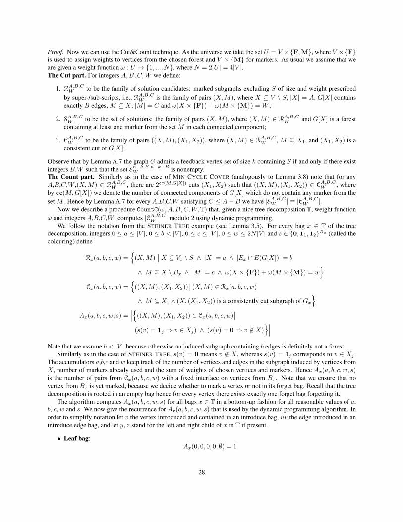
Proof. Now we can use the Cut&Count technique. As the universe we take the set U = V ×F,M, where V ×Fis used to assign weights to vertices from the chosen forest and V × M for markers. As usual we assume that weare given a weight function ω : U → 1, ..., N, where N = 2|U | = 4|V |.The Cut part. For integers A,B,C,W we define:
1. RA,B,CW to be the family of solution candidates: marked subgraphs excluding S of size and weight prescribed
by super-/sub-scripts, i.e., RA,B,CW is the family of pairs (X,M), where X ⊆ V \ S, |X| = A, G[X] containsexactly B edges, M ⊆ X , |M | = C and ω(X × F) + ω(M × M) = W ;
2. SA,B,CW to be the set of solutions: the family of pairs (X,M), where (X,M) ∈ R
A,B,CW and G[X] is a forest
containing at least one marker from the set M in each connected component;
3. CA,B,CW to be the family of pairs ((X,M), (X1, X2)), where (X,M) ∈ R
A,B,CW , M ⊆ X1, and (X1, X2) is a
consistent cut of G[X].
Observe that by Lemma A.7 the graph G admits a feedback vertex set of size k containing S if and only if there existintegers B,W such that the set Sn−k,B,n−k−BW is nonempty.The Count part. Similarly as in the case of MIN CYCLE COVER (analogously to Lemma 3.8) note that for anyA,B,C,W ,(X,M) ∈ R
A,B,CW , there are 2cc(M,G[X]) cuts (X1, X2) such that ((X,M), (X1, X2)) ∈ C
A,B,CW , where
by cc(M,G[X]) we denote the number of connected components of G[X] which do not contain any marker from theset M . Hence by Lemma A.7 for every A,B,C,W satisfying C ≤ A−B we have |SA,B,CW | ≡ |CA,B,CW |.
Now we describe a procedure CountC(ω,A,B,C,W,T) that, given a nice tree decomposition T, weight functionω and integers A,B,C,W , computes |CA,B,CW | modulo 2 using dynamic programming.
We follow the notation from the STEINER TREE example (see Lemma 3.5). For every bag x ∈ T of the treedecomposition, integers 0 ≤ a ≤ |V |, 0 ≤ b < |V |, 0 ≤ c ≤ |V |, 0 ≤ w ≤ 2N |V | and s ∈ 0,11,12Bx (called thecolouring) define
Rx(a, b, c, w) =
(X,M)∣∣ X ⊆ Vx \ S ∧ |X| = a ∧ |Ex ∩ E(G[X])| = b
∧ M ⊆ X \Bx ∧ |M | = c ∧ ω(X × F) + ω(M × M) = w
Cx(a, b, c, w) =
((X,M), (X1, X2))∣∣ (X,M) ∈ Rx(a, b, c, w)
∧ M ⊆ X1 ∧ (X, (X1, X2)) is a consistently cut subgraph of Gx
Ax(a, b, c, w, s) =∣∣∣((X,M), (X1, X2)) ∈ Cx(a, b, c, w)
∣∣(s(v) = 1j ⇒ v ∈ Xj) ∧ (s(v) = 0⇒ v 6∈ X)
∣∣∣Note that we assume b < |V | because otherwise an induced subgraph containing b edges is definitely not a forest.
Similarly as in the case of STEINER TREE, s(v) = 0 means v /∈ X , whereas s(v) = 1j corresponds to v ∈ Xj .The accumulators a,b,c and w keep track of the number of vertices and edges in the subgraph induced by vertices fromX , number of markers already used and the sum of weights of chosen vertices and markers. Hence Ax(a, b, c, w, s)is the number of pairs from Cx(a, b, c, w) with a fixed interface on vertices from Bx. Note that we ensure that novertex from Bx is yet marked, because we decide whether to mark a vertex or not in its forget bag. Recall that the treedecomposition is rooted in an empty bag hence for every vertex there exists exactly one forget bag forgetting it.
The algorithm computes Ax(a, b, c, w, s) for all bags x ∈ T in a bottom-up fashion for all reasonable values of a,b, c, w and s. We now give the recurrence for Ax(a, b, c, w, s) that is used by the dynamic programming algorithm. Inorder to simplify notation let v the vertex introduced and contained in an introduce bag, uv the edge introduced in anintroduce edge bag, and let y, z stand for the left and right child of x in T if present.
• Leaf bag:Ax(0, 0, 0, 0, ∅) = 1
28
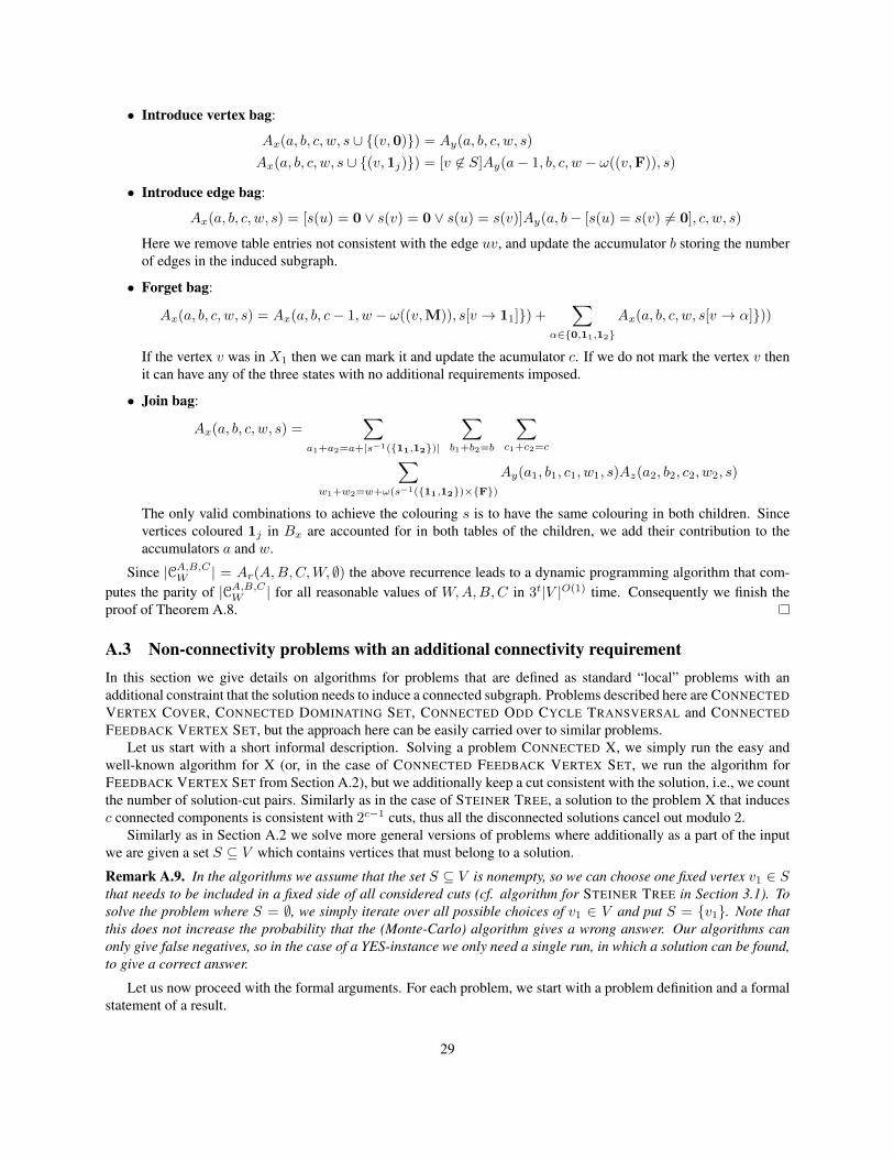
• Introduce vertex bag:
Ax(a, b, c, w, s ∪ (v,0)) = Ay(a, b, c, w, s)
Ax(a, b, c, w, s ∪ (v,1j)) = [v 6∈ S]Ay(a− 1, b, c, w − ω((v,F)), s)
• Introduce edge bag:
Ax(a, b, c, w, s) = [s(u) = 0 ∨ s(v) = 0 ∨ s(u) = s(v)]Ay(a, b− [s(u) = s(v) 6= 0], c, w, s)
Here we remove table entries not consistent with the edge uv, and update the accumulator b storing the numberof edges in the induced subgraph.
• Forget bag:
Ax(a, b, c, w, s) = Ax(a, b, c− 1, w − ω((v,M)), s[v → 11]) +∑
α∈0,11,12Ax(a, b, c, w, s[v → α]))
If the vertex v was in X1 then we can mark it and update the acumulator c. If we do not mark the vertex v thenit can have any of the three states with no additional requirements imposed.
• Join bag:
Ax(a, b, c, w, s) =∑
a1+a2=a+|s−1(11,12)|
∑b1+b2=b
∑c1+c2=c∑
w1+w2=w+ω(s−1(11,12)×F)Ay(a1, b1, c1, w1, s)Az(a2, b2, c2, w2, s)
The only valid combinations to achieve the colouring s is to have the same colouring in both children. Sincevertices coloured 1j in Bx are accounted for in both tables of the children, we add their contribution to theaccumulators a and w.
Since |CA,B,CW | = Ar(A,B,C,W, ∅) the above recurrence leads to a dynamic programming algorithm that com-putes the parity of |CA,B,CW | for all reasonable values of W,A,B,C in 3t|V |O(1) time. Consequently we finish theproof of Theorem A.8.
A.3 Non-connectivity problems with an additional connectivity requirementIn this section we give details on algorithms for problems that are defined as standard “local” problems with anadditional constraint that the solution needs to induce a connected subgraph. Problems described here are CONNECTEDVERTEX COVER, CONNECTED DOMINATING SET, CONNECTED ODD CYCLE TRANSVERSAL and CONNECTEDFEEDBACK VERTEX SET, but the approach here can be easily carried over to similar problems.
Let us start with a short informal description. Solving a problem CONNECTED X, we simply run the easy andwell-known algorithm for X (or, in the case of CONNECTED FEEDBACK VERTEX SET, we run the algorithm forFEEDBACK VERTEX SET from Section A.2), but we additionally keep a cut consistent with the solution, i.e., we countthe number of solution-cut pairs. Similarly as in the case of STEINER TREE, a solution to the problem X that inducesc connected components is consistent with 2c−1 cuts, thus all the disconnected solutions cancel out modulo 2.
Similarly as in Section A.2 we solve more general versions of problems where additionally as a part of the inputwe are given a set S ⊆ V which contains vertices that must belong to a solution.
Remark A.9. In the algorithms we assume that the set S ⊆ V is nonempty, so we can choose one fixed vertex v1 ∈ Sthat needs to be included in a fixed side of all considered cuts (cf. algorithm for STEINER TREE in Section 3.1). Tosolve the problem where S = ∅, we simply iterate over all possible choices of v1 ∈ V and put S = v1. Note thatthis does not increase the probability that the (Monte-Carlo) algorithm gives a wrong answer. Our algorithms canonly give false negatives, so in the case of a YES-instance we only need a single run, in which a solution can be found,to give a correct answer.
Let us now proceed with the formal arguments. For each problem, we start with a problem definition and a formalstatement of a result.
29

A.3.1 CONNECTED VERTEX COVER
CONSTRAINED CONNECTED VERTEX COVERInput: An undirected graph G = (V,E), a subset S ⊆ V and an integer kQuestion: Does there exist such a subset X ⊆ V of cardinality k that S ⊆ X , G[X] is connected and each edgee ∈ E is incident with at least one vertex from X?
Theorem A.10. There exists a Monte-Carlo algorithm that given a tree decomposition of width t solves CON-STRAINED CONNECTED VERTEX COVER in 3t|V |O(1) time. The algorithm cannot give false positives and maygive false negatives with probability at most 1/2.
There exists an easy proof of Theorem A.10 by a reduction to the STEINER TREE problem — we subdivide alledges of the graph G using terminals and add pendant terminals to S. Such a transformation does not change thetreewidth of the graph by more than one. Nonetheless we prove the theorem by a direct application of the Cut&Counttechnique, in a similar manner as for the STEINER TREE problem in Section 3.1. Our motivation for choosing thesecond approach is that we need it to develop an algorithm for CONNECTED VERTEX COVER parameterized by thesolution size in Appendix B which relies on the algorithm we describe in the proof.
Proof. We use the Cut&Count technique. As the universe for Algorithm 1 we take the vertex set U = V . Recall thatwe generate a random weight function ω : U → 1, 2, . . . , N, taking N = 2|U | = 2|V |. By Remark A.9 we mayassume that S 6= ∅ and we may choose one fixed vertex v1 ∈ S.The Cut part. For an integer W we define:
1. RW to be the family of solution candidates of size k and weight W : RW is the family of sets X ⊆ V such thatS ⊆ X , |X| = k, ω(X) = W and X is a vertex cover of G;
2. SW to be the family of solutions of size k and weight W , that is sets X ∈ RW such that G[X] is connected;
3. CW to be the family of pairs (X, (X1, X2)), where X ∈ RW , v1 ∈ X1 and (X1, X2) is a consistent cut ofG[X].
The Count part. Similarly as in the case of STEINER TREE we note that by Lemma 3.3 for each X ∈ RW there exist2cc(G[X])−1 consistent cuts of G[X], thus for any W we have |SW | ≡ |CW |.
To finish the proof we need to describe a procedure CountC(ω,W,T) that, given a nice tree decomposition T,weight function ω and an integer W , computes |CW | modulo 2.
As usual we use dynamic programming. We follow the notation from the STEINER TREE example (see Lemma3.5). For every bag x ∈ T of the tree decomposition, integers 0 ≤ i ≤ |V |, 0 ≤ w ≤ N |V | and s ∈ 0,11,12Bx(called the colouring) define
Rx(i, w) =X ⊆ Vx
∣∣ (S ∩ Vx) ⊆ X ∧ |X| = i ∧ ω(X) = w ∧ X is a vertex cover of Gx
Cx(i, w) =
(X, (X1, X2))∣∣ X ∈ Rx(i, w) ∧ (X, (X1, X2)) is a consistently cut subgraph of Gx
∧ (v1 ∈ Vx ⇒ v1 ∈ X1)
Ax(i, w, s) =∣∣∣(X, (X1, X2)) ∈ Cx(i, w)
∣∣ (s(v) = 1j ⇒ v ∈ Xj) ∧ (s(v) = 0⇒ v 6∈ X)∣∣∣
Similarly as in the case of STEINER TREE, s(v) = 0 means v /∈ X , whereas s(v) = 1j corresponds to v ∈ Xj .The accumulators i and w keep track of the number of vertices in the solution and their weights, respectively. HenceAx(i, w, s) is the number of pairs from C of candidate solutions and consident cuts on Gx, with fixed size, weight andinterface on vertices from Bx.
The algorithm computes Ax(i, w, s) for all bags x ∈ T in a bottom-up fashion for all reasonable values of i, wand s. We now give the recurrence for Ax(i, w, s) that is used by the dynamic programming algorithm. In order tosimplify notation denote by v the vertex introduced and contained in an introduce bag, by uv the edge introduced inan introduce edge bag, and let y, z be the left and right child of x in T if present.
30
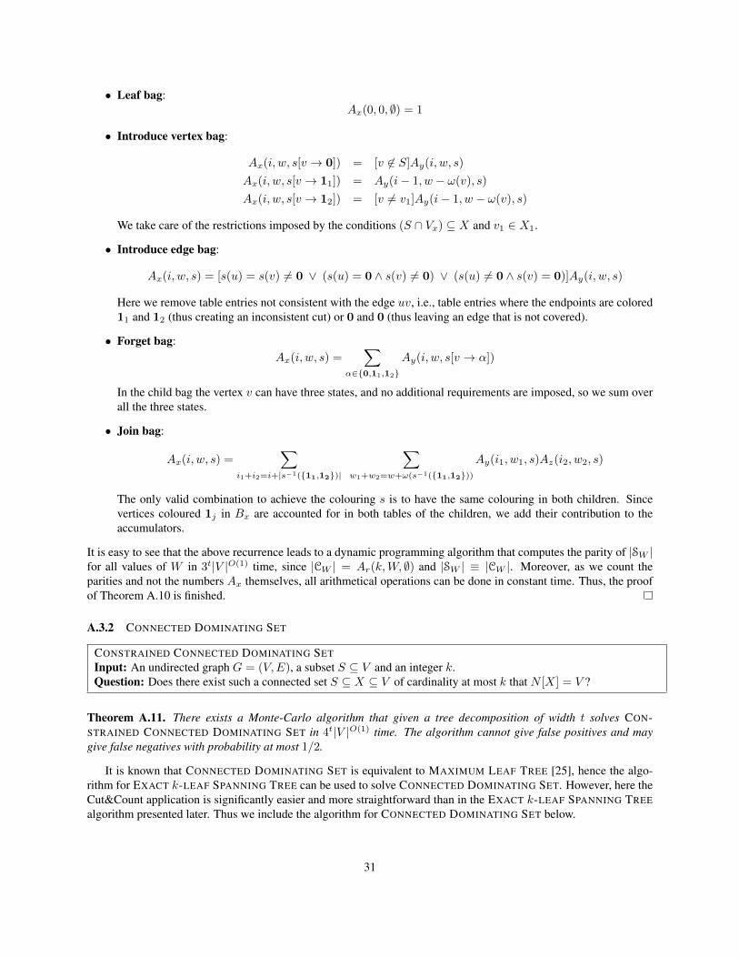
• Leaf bag:Ax(0, 0, ∅) = 1
• Introduce vertex bag:
Ax(i, w, s[v → 0]) = [v 6∈ S]Ay(i, w, s)
Ax(i, w, s[v → 11]) = Ay(i− 1, w − ω(v), s)
Ax(i, w, s[v → 12]) = [v 6= v1]Ay(i− 1, w − ω(v), s)
We take care of the restrictions imposed by the conditions (S ∩ Vx) ⊆ X and v1 ∈ X1.
• Introduce edge bag:
Ax(i, w, s) = [s(u) = s(v) 6= 0 ∨ (s(u) = 0 ∧ s(v) 6= 0) ∨ (s(u) 6= 0 ∧ s(v) = 0)]Ay(i, w, s)
Here we remove table entries not consistent with the edge uv, i.e., table entries where the endpoints are colored11 and 12 (thus creating an inconsistent cut) or 0 and 0 (thus leaving an edge that is not covered).
• Forget bag:Ax(i, w, s) =
∑α∈0,11,12
Ay(i, w, s[v → α])
In the child bag the vertex v can have three states, and no additional requirements are imposed, so we sum overall the three states.
• Join bag:
Ax(i, w, s) =∑
i1+i2=i+|s−1(11,12)|
∑w1+w2=w+ω(s−1(11,12))
Ay(i1, w1, s)Az(i2, w2, s)
The only valid combination to achieve the colouring s is to have the same colouring in both children. Sincevertices coloured 1j in Bx are accounted for in both tables of the children, we add their contribution to theaccumulators.
It is easy to see that the above recurrence leads to a dynamic programming algorithm that computes the parity of |SW |for all values of W in 3t|V |O(1) time, since |CW | = Ar(k,W, ∅) and |SW | ≡ |CW |. Moreover, as we count theparities and not the numbers Ax themselves, all arithmetical operations can be done in constant time. Thus, the proofof Theorem A.10 is finished.
A.3.2 CONNECTED DOMINATING SET
CONSTRAINED CONNECTED DOMINATING SETInput: An undirected graph G = (V,E), a subset S ⊆ V and an integer k.Question: Does there exist such a connected set S ⊆ X ⊆ V of cardinality at most k that N [X] = V ?
Theorem A.11. There exists a Monte-Carlo algorithm that given a tree decomposition of width t solves CON-STRAINED CONNECTED DOMINATING SET in 4t|V |O(1) time. The algorithm cannot give false positives and maygive false negatives with probability at most 1/2.
It is known that CONNECTED DOMINATING SET is equivalent to MAXIMUM LEAF TREE [25], hence the algo-rithm for EXACT k-LEAF SPANNING TREE can be used to solve CONNECTED DOMINATING SET. However, here theCut&Count application is significantly easier and more straightforward than in the EXACT k-LEAF SPANNING TREEalgorithm presented later. Thus we include the algorithm for CONNECTED DOMINATING SET below.
31

Proof of Theorem A.11. We use the Cut&Count technique. As the universe for Algorithm 1 we take the vertex setU = V . Recall that we generate a random weight function ω : U → 1, 2, . . . , N, taking N = 2|U | = 2|V |. ByRemark A.9 we may assume that S 6= ∅ and we may choose one fixed vertex v1 ∈ S.The Cut part. For an integer W we define:
1. RW to be the family of solution candidates of size k and weight W : RW is the family of sets X ⊆ V such thatS ⊆ X , |X| = k, ω(X) = W and N [X] = V .
2. SW to be the family of solutions of size k and weight W , that is sets X ∈ RW such that G[X] is connected;
3. CW to be the family of pairs (X, (X1, X2)), where X ∈ RW , and (X1, X2) is a consistent cut of G[X].
The Count part. As before we note that by Lemma 3.3 for each X ∈ RW there exist 2cc(G[X])−1 consistent cuts ofG[X], thus for any W we have |SW | ≡ |CW |. What remains is to describe a procedure CountC(ω,W,T) that, given anice tree decomposition T, weight function ω and an integer W , computes |CW | modulo 2.
As usual we use dynamic programming. We follow the notation from the STEINER TREE example (see Lemma3.5). For every bag x ∈ T of the tree decomposition, integers 0 ≤ i ≤ |V |, 0 ≤ w ≤ N |V | and s ∈ 0N ,0Y ,11,12Bx(called the colouring) define
Rx(i, w) =X ⊆ Vx
∣∣ (S ∩ Vx) ⊆ X ∧ |X| = i ∧ ω(X) = w ∧ NGx [X] = Vx \ s−1(0N )
Cx(i, w) =
(X, (X1, X2))∣∣ X ∈ Rx(i, w) ∧ (X, (X1, X2)) is a consistently cut subgraph of Gx
∧ (v1 ∈ Vx ⇒ v1 ∈ X1)
Ax(i, w, s) =∣∣∣(X, (X1, X2)) ∈ Cx(i, w)
∣∣ (s(v) = 1j ⇒ v ∈ Xj)
∧ (s(v) = 0Y ⇒ v ∈ NGx(X)) ∧ (s(v) = 0N ⇒ v 6∈ NGx [X]∣∣∣
Here s(v) = 0Y means v /∈ X and v is dominated by X in Gx, s(v) = 0N means v /∈ X and v is not dominated byX in Gx, whereas s(v) = 1j corresponds to v ∈ Xj . The accumulators i and w keep track of the number of verticesin the solution and their weights, respectively. Hence Ax(i, w, s) is the number of pairs from C of candidate solutionsand consistent cuts on Gx, with fixed size, weight and interface on vertices from Bx.
The algorithm computes Ax(i, w, s) for all bags x ∈ T in a bottom-up fashion for all reasonable values of i, wand s. We now give the recurrence for Ax(i, w, s) that is used by the dynamic programming algorithm. As usual, vdenotes the vertex introduced and contained in an introduce bag, uv the edge introduced in an introduce edge bag,while y and z denote the left and right child of x in T, if present.
• Leaf bag:Ax(0, 0, ∅) = 1
• Introduce vertex bag:
Ax(i, w, s[v → 0N ]) = [v 6∈ S]Ay(i, w, s)
Ax(i, w, s[v → 0Y ]) = 0
Ax(i, w, s[v → 11]) = Ay(i− 1, w − ω(v), s)
Ax(i, w, s[v → 12]) = [v 6= v1]Ay(i− 1, w − ω(v), s)
We take care of restrictions imposed by conditions (S ∩ Vx) ⊆ X and v1 ∈ X1. Note that at the moment ofintroducing v there are no edges incident to v in Gx, thus v cannot dominated, but not chosen.
32
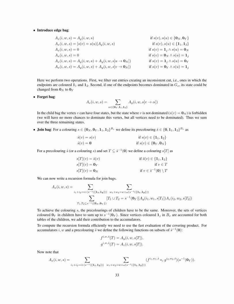
• Introduce edge bag:
Ax(i, w, s) = Ay(i, w, s) if s(v), s(u) ∈ 0N ,0Y Ax(i, w, s) = [s(v) = s(u)]Ay(i, w, s) if s(v), s(u) ∈ 11,12Ax(i, w, s) = 0 if s(v) = 1j ∧ s(u) = 0N
Ax(i, w, s) = 0 if s(v) = 0N ∧ s(u) = 1j
Ax(i, w, s) = Ay(i, w, s) +Ay(i, w, s[u→ 0N ]) if s(v) = 1j ∧ s(u) = 0Y
Ax(i, w, s) = Ay(i, w, s) +Ay(i, w, s[v → 0N ]) if s(v) = 0Y ∧ s(u) = 1j
Here we perform two operations. First, we filter out entries creating an inconsistent cut, i.e., ones in which theendpoints are coloured 11 and 12. Second, if one of the endpoints becomes dominated in Gx, its state could bechanged from 0N to 0Y
• Forget bag:Ax(i, w, s) =
∑α∈0Y ,11,12
Ay(i, w, s[v → α])
In the child bag the vertex v can have four states, but the state where v is not dominated (s(v) = 0N ) is forbidden(we will have no more chances to dominate this vertex, but all vertices need to be dominated). Thus we sumover the three remaining states.
• Join bag: For a colouring s ∈ 0N ,0Y ,11,12Bx we define its precolouring s ∈ 0,11,12Bx as
s(v) = s(v) if s(v) ∈ 11,12s(v) = 0 if s(v) ∈ 0Y ,0N
For a precolouring s (or a colouring s) and set T ⊆ s−1(0) we define a colouring s[T ] as
s[T ](v) = s(v) if s(v) ∈ 11,12s[T ](v) = 0Y if v ∈ Ts[T ](v) = 0N if v ∈ s−1(0) \ T
We can now write a recursion formula for join bags.
Ax(i, w, s) =∑
i1+i2=i+|s−1(11,12)|
∑w1+w2=w+ω(s−1(11,12))∑
T1,T2⊆s−1(0N ,0Y )[T1 ∪ T2 = s−1(0Y )]Ay(i1, w1, s[T1])Az(i2, w2, s[T2])
To achieve the colouring s, the precolourings of children have to be the same. Moreover, the sets of verticescoloured 0Y in children have to sum up to s−1(0Y ). Since vertices coloured 1j in Bx are accounted for bothtables of the children, we add their contribution to the accumulators.
To compute the recursion formula efficiently we need to use the fast evaluation of the covering product. Foraccumulators i, w and a precolouring s we define the following functions on subsets of s−1(0):
f i,w,s(T ) = Ay(i, w, s[T ]),
gi,w,s(T ) = Az(i, w, s[T ]).
Now note that
Ax(i, w, s) =∑
i1+i2=i+|s−1(11,12)|
∑w1+w2=w+ω(s−1(11,12))
(f i1,w1,s ∗c gi2,w2,s)(s−1(0Y )).
33

By Theorem A.2, for fixed accumulators i1, w1, i2, w2 and a precolouring s the term
(f i1,w1,s ∗c gi2,w2,s)(s−1(0Y ))
can be computed in time 2|s−1(0)||s−1(0)|O(1) at once for all colourings s with precolouring s. Thus, the total
time consumed by the evaluation of Ax is bounded by
|V |O(1)∑
s∈0,11,12Bx2|s−1(0)| = 4|Bx||V |O(1).
It is easy to see that the above recurrence leads to a dynamic programming algorithm that computes the parity of |SW |for all values ofW in 4t|V |O(1) time, since |CW | = Ar(k,W, ∅) and |SW | ≡ |CW |. Moreover, as we count the paritiesand not the numbers Ax themselves, all arithmetical operations (in particular, the ring operations in the convolutionsused in join bags) can be done in constant time. Thus, the proof of Theorem A.11 is finished.
A.3.3 CONNECTED ODD CYCLE TRANSVERSAL
CONSTRAINED CONNECTED ODD CYCLE TRANSVERSALInput: An undirected graph G = (V,E), a subset S ⊆ V and an integer kQuestion: Does there exist a subset X ⊆ V of cardinality k, such that S ⊆ X , G[X] is connected and G[V \X] isbipartite?
Theorem A.12. There exists a Monte-Carlo algorithm that given a tree decomposition of width t solves CON-STRAINED CONNECTED ODD CYCLE TRANSVERSAL in 4t|V |O(1) time. The algorithm cannot give false positivesand may give false negatives with probability at most 1/2.
Proof. We use the Cut&Count technique. As the universe for Algorithm 1 we take U = V × X,L, i.e., for eachvertex v ∈ V we generate two weights ω((v,X)) and ω((v,L)). Recall that we generate a random weight functionω : U → 1, 2, . . . , N, taking N = 2|U | = 4|V |. By Remark A.9 we may assume that S 6= ∅ and we may chooseone fixed vertex v1 ∈ S.The Cut part. To make use of the well-known algorithm for ODD CYCLE TRANSVERSAL parameterized by treewidth,we need to define a solution not only as a set X , but we need to add a proof that G[V \X] is bipartite (i.e., a partitionof V \X into two independent sets). Formally, for an integer W we define:
1. RW to be the family of pairs (X,L), where |X| = k, ω(X × X ∪ L× L) = W , S ⊆ X , X ∩ L = ∅ andL and V \ (X ∪ L) are independent sets in G;
2. SW to be the family of pairs (X,L) ∈ RW such that G[X] is connected;
3. CW to be the family of pairs ((X,L), (X1, X2)), where (X,L) ∈ RW , v1 ∈ X1 and (X1, X2) is a consistentcut of G[X].
Note that for a single set X ⊆ V there may exist many proofs L that G[V \ X] is bipartite. We consider all pairs(X,L) as different solutions and solution candidates. To compute weight, each pair (X,L) is represented as X ×X ∪ L× L ⊆ U , thus each pair (X,L) corresponds to a different subset of the weight domain U .The Count part. Similarly as in the case of STEINER TREE we note that by Lemma 3.3 for each (X,L) ∈ RW thereexist 2cc(G[X])−1 consistent cuts of G[X], thus for any W we have |SW | ≡ |CW |.
To finish the proof we need to describe a procedure CountC(ω,W,T) that, given a nice tree decomposition T,weight function ω and an integer W , computes |CW | modulo 2.
As usual we use dynamic programming. We follow the notation from the STEINER TREE example (see Lemma3.5). For every bag x ∈ T of the tree decomposition, integers 0 ≤ i ≤ |V |, 0 ≤ w ≤ N |V | and s ∈ 0L,0R,11,12Bx
34

(called the colouring) define
Rx(i, w) =
(X,L)∣∣ X,L ⊆ Vx ∧ X ∩ L = ∅ ∧ (S ∩ Vx) ⊆ X ∧ |X| = i
∧ ω(X × X ∪ L× L) = w ∧ L and Vx \ (X ∪ L) are independent sets in Gx
Cx(i, w) =
((X,L), (X1, X2))∣∣ (X,L) ∈ Rx(i, w) ∧ (X, (X1, X2)) is a consistently cut subgraph of Gx
∧ (v1 ∈ Vx ⇒ v1 ∈ X1)
Ax(i, w, s) =∣∣∣((X,L), (X1, X2)) ∈ Cx(i, w)
∣∣ (s(v) = 1j ⇒ v ∈ Xj)
∧ (s(v) = 0L ⇒ v ∈ L) ∧ (s(v) = 0R ⇒ v 6∈ X ∪ L)∣∣∣
Here we plan L and V \ (X ∪ L) to be a bipartition of G[V \ X]; s(v) = 0L and 0R mean v is on the left or rightside of this bipartition, respectively, while s(v) = 1j means v is in the odd cycle transversal, and on the appropriateside of the cut. The accumulators i and w keep track of the number of vertices in X and the weight of the pair (X,L),respectively. Hence Ax(i, w, s) is the number of pairs from C of candidate solutions and consistent cuts on Gx, withfixed size, weight and interface on vertices from Bx.
The algorithm computes Ax(i, w, s) for all bags x ∈ T in a bottom-up fashion for all reasonable values of i, wand s. We now give the recurrence for Ax(i, w, s) that is used by the dynamic programming algorithm. As always letv stand for the vertex introduced and contained in an introduce bag, uv for the edge introduced in an introduce edgebag, and y, z for the left and right child of x in T if present.
• Leaf bag:Ax(0, 0, ∅) = 1
• Introduce vertex bag:
Ax(i, w, s[v → 0L]) = [v 6∈ S]Ay(i, w − ω((v,L)), s)
Ax(i, w, s[v → 0R]) = [v 6∈ S]Ay(i, w, s)
Ax(i, w, s]v → 11]) = Ay(i− 1, w − ω((v,X)), s)
Ax(i, w, s[v → 12]) = [v 6= v1]Ay(i− 1, w − ω((v,X)), s)
We take care of restrictions imposed by conditions (S ∩ Vx) ⊆ X and v1 ∈ X1.
• Introduce edge bag:
Ax(i, w, s) = 0 if s(u), s(v) = 11,12Ax(i, w, s) = 0 if s(u) = s(v) ∈ 0L,0RAx(i, w, s) = Ay(i, w, s) otherwise
Here we remove table entries not consistent with the edge uv, i.e., table entries where the endpoints are coloured11 and 12 (thus creating an inconsistent cut) or both coloured 0L or both coloured 0R (thus introducing an edgein Gx[L] or Gx[Vx \ (X ∪ L)]).
• Forget bag:Ax(i, w, s) =
∑α∈0L,0R,11,12
Ay(i, w, s[v → α])
In the child bag the vertex v can have four states, and no additional requirements are imposed, so we sum overall the four states.
35

• Join bag:
Ax(i, w, s) =∑
i1+i2=i+|s−1(11,12)|
∑w1+w2=w+ω(s−1(11,12)×X∪s−1(0L)×L)
Ay(i1, w1, s)Az(i2, w2, s)
The only valid combinations to achieve the colouring s is to have the same colouring in both children. Sincevertices coloured 1j and 0L in Bx are accounted for in both tables of the children, we add their contribution tothe accumulators.
It is easy to see that the above recurrence leads to a dynamic programming algorithm that computes the parity of |SW |for all values of W in 4t|V |O(1) time, since |CW | = Ar(k,W, ∅) and |SW | ≡ |CW |. Moreover, as we count theparities and not the numbers Ax themselves, all arithmetical operations can be done in constant time. Thus, the proofof Theorem A.12 is finished.
A.3.4 CONNECTED FEEDBACK VERTEX SET
CONSTRAINED CONNECTED FEEDBACK VERTEX SETInput: An undirected graph G = (V,E), a subset S ⊆ V and an integer k.Question: Does there exist a set Y ⊆ V of cardinality k such that S ⊆ Y , G[Y ] is connected andG[V \Y ] is a forest?
Theorem A.13. There exists a Monte-Carlo algorithm that given a tree decomposition of width t solves the CON-STRAINED CONNECTED FEEDBACK VERTEX SET problem in 4t|V |O(1) time. The algorithm cannot give false posi-tives and may give false negatives with probability at most 1/2.
Proof. We use the Cut&Count technique. The idea is as in the previous algorithms in this subsection: we use thedynamic programming for FEEDBACK VERTEX SET, additionally keeping a cut consistent with the solution Y . How-ever, in the previous subsections the base dynamic programming algorithms were the easy, naive ones. Here we needto use the Cut&Count based algorithm from Section A.2. Thus, we attach to a solution candidate two cuts: one ofG[Y ], and second of G[V \ Y ].
As a universe we take the set U = V × F,M, where V × F is used to assign weights to vertices fromthe chosen forest G[V \ Y ] and V × M for markers. As usual we assume that we are given a weight functionω : U → 1, ..., N, where N = 2|U | = 4|V |. By Remark A.9 we assume S 6= ∅ and we fix one vertex v1 ∈ S.The Cut part. For integers A,B,C,W we define:
1. RA,B,CW to be the family of solution candidates, that is a marked subgraphs excluding S of size and weight
prescribed by super-/sub-scripts, i.e., RA,B,CW is the family of pairs (X,M), where X ⊆ V \ S, |X| = A, G[X]contains exactly B edges, M ⊆ X , |M | = C and ω(X × F) + ω(M × M) = W ;
2. SA,B,CW to be the set of solutions, that is the family of pairs (X,M), where (X,M) ∈ R
A,B,CW , where G[X] is a
forest containing at least one marker from the set M in each connected component and G[V \X] is connected;
3. CA,B,CW to be the family of triples ((X,M), (X1, X2), (Y1, Y2)), where (X,M) ∈ R
A,B,CW , M ⊆ X1, (X1, X2)
is a consistent cut of G[X], v1 ∈ Y1 and (Y1, Y2) is a consistent cut of G[V \X].
Observe that by Lemma A.7 the graph G admits a connected feedback vertex set of size k containing S if and only ifthere exist integers B,W such that the set Sn−k,B,n−k−BW is nonempty.The Count part. Similarly as in the case of STEINER TREE we note that by Lemma 3.3 for any A,B,C,W ,(X,M) ∈RA,B,CW , there exist 2cc(G[V \X])−1 cuts (Y1, Y2) that are consistent cuts of G[V \X] and v1 ∈ Y1. Moreover, similarly
as in the case of MIN CYCLE COVER (analogously to Lemma 3.8) note that there are 2cc(M,G[X]) cuts (X1, X2) thatare consistent with G[X] and M ⊆ X1, where by cc(M,G[X]) we denote the number of connected componentsof G[X] which do not contain any marker from the set M . Thus for any A,B,C,W ,(X,M) ∈ R
A,B,CW , there are
2cc(G[V \X])−1+cc(M,G[X]) triples ((X,M), (X1, X2), (Y1, Y2)) ∈ CA,B,CW . Hence by Lemma A.7 for everyA,B,C,W
satisfying C ≤ A−B we have |SA,B,CW | ≡ |CA,B,CW |.
36

Now we describe a procedure CountC(ω,A,B,C,W,T) that, given a nice tree decomposition T, weight functionω and integers A,B,C,W , computes |CA,B,CW | modulo 2 using dynamic programming.
We follow the notation from the STEINER TREE example (see Lemma 3.5). For every bag x ∈ T of the treedecomposition, integers 0 ≤ a ≤ |V |, 0 ≤ b < |V |, 0 ≤ c ≤ |V |, 0 ≤ w ≤ 2N |V | and s ∈ 01,02,11,12Bx (calledthe colouring) define
Rx(a, b, c, w) =
(X,M)∣∣ X ⊆ Vx \ S ∧ |X| = a ∧ |Ex ∩ E(G[X])| = b
∧ M ⊆ X \Bx ∧ |M | = c ∧ ω(X × F) + ω(M × M) = w
Cx(a, b, c, w) =
((X,M), (X1, X2), (Y1, Y2))∣∣ (X,M) ∈ Rx(a, b, c, w)
∧ M ⊆ X1 ∧ (X, (X1, X2)) is a consistently cut subgraph of Gx
∧ (v1 ∈ Vx ⇒ v1 ∈ Y1) ∧ (Vx \X, (Y1, Y2)) is a consistently cut subgraph of Gx
Ax(a, b, c, w, s) =∣∣∣((X,M), (X1, X2), (Y1, Y2)) ∈ Cx(a, b, c, w)
∣∣(s(v) = 1j ⇒ v ∈ Xj) ∧ (s(v) = 0jv ∈ Yj)
∣∣∣Note that we assume b < |V | because otherwise an induced subgraph containing b edges is definitely not a forest.
Similarly as in the case of STEINER TREE, s(v) = 0j means v ∈ Yj , whereas s(v) = 1j corresponds to v ∈ Xj .The accumulators a,b,c and w keep track of the number of vertices and edges in the subgraph induced by vertices fromX , number of markers already used and the sum of weights of chosen vertices and markers. Hence Ax(a, b, c, w, s) isthe number of triples from Cx(a, b, c, w) with a fixed interface on vertices from Bx. Note that we ensure that no vertexfrom Bx is yet marked, because we decide whether to mark a vertex or not in its forget bag.
The algorithm computes Ax(a, b, c, w, s) for all bags x ∈ T in a bottom-up fashion for all reasonable values of a,b, c, w and s. We now give the recurrence for Ax(a, b, c, w, s) that is used by the dynamic programming algorithm.As in the previous sections by v we denote the vertex introduced and contained in an introduce bag, by uv the edgeintroduced in an introduce edge bag, and by y, z for the left and right child of x in T if present.
• Leaf bag:Ax(0, 0, 0, 0, ∅) = 1
• Introduce vertex bag:
Ax(a, b, c, w, s[v → 01]) = Ay(a, b, c, w, s)
Ax(a, b, c, w, s[v → 02]) = [v 6= v1]Ay(a, b, c, w, s)
Ax(a, b, c, w, s[v → 1j ]) = [v 6∈ S]Ay(a− 1, b, c, w − ω((v,F)), s)
Here we take care of the constraints S ∩X = ∅ and v1 ∈ Y1.
• Introduce edge bag:
Ax(a, b, c, w, s) = 0 if s(v), s(u) = 01,02Ax(a, b, c, w, s) = 0 if s(v), s(u) = 11,12Ax(a, b, c, w, s) = Ay(a, b− 1, c, w, s) if s(v) = s(u) ∈ 11,12Ax(a, b, c, w, s) = Ay(a, b, c, w, s) otherwise
Here we remove table entries not consistent with the edge uv (i.e., creating an inconsistent cut, either (X1, X2)or (Y1, Y2)), and update the accumulator b storing the number of edges in G[X].
37

• Forget bag:
Ax(a, b, c, w, s) = Ay(a, b, c− 1, w − ω((v,M)), s[v → 11]) +∑
α∈01,02,11,12Ay(a, b, c, w, s[v → α]))
If the vertex v was in X1 then we can mark it and update the accumulator c. If we do not mark the vertex v thenit can have any of the four states with no additional requirements imposed.
• Join bag:
Ax(i, w, s) =∑
a1+a2=a+|s−1(11,12)|
∑b1+b2=b
∑c1+c2=c∑
w1+w2=w+ω(s−1(11,12)×F)Ay(a1, b1, c1, w1, s)Az(a2, b2, c2, w2, s)
The only valid combinations to achieve the colouring s is to have the same colouring in both children. Sincevertices coloured 1j in Bx are accounted for in both tables of the children, we add their contribution to theaccumulators a and w.
Since |CA,B,CW | = Ar(A,B,C,W, ∅) the above recurrence leads to a dynamic programming algorithm that com-putes the parity of |CA,B,CW | for all reasonable values of W,A,B,C in 4tnO(1) time. Consequently we finish the proofof Theorem A.13.
A.4 Longest Cycles, Paths and Cycle CoversIn this section we consider the following three problems, both in the directed and undirected setting.
(DIRECTED) MIN CYCLE COVERInput: An undirected graph G = (V,E) (or a directed graph D = (V,A)) and an integer k.Question: Can the vertices of G (D) be covered with at most k vertex disjoint (directed) cycles?
(DIRECTED) LONGEST CYCLEInput: An undirected graph G = (V,E) (or a directed graph D = (V,A)) and an integer k.Question: Does there exist a (directed) simple cycle of length k in G (D)?
(DIRECTED) LONGEST PATHInput: An undirected graph G = (V,E) (or a directed graph D = (V,A)) and an integer k.Question: Does there exist a (directed) simple path of length k in G (D)?
We capture all three problems in the following artificial one.
(DIRECTED) PARTIAL CYCLE COVERInput: An undirected graph G = (V,E) (or a directed graph D = (V,A)) and integers k and `.Question: Does there exist a family of at most k vertex disjoint (directed) cycles inG (D) that cover exactly ` vertices?
Note that for k = 1 the above problem becomes LONGEST CYCLE, whereas for ` = |V | it becomes MIN CYCLECOVER. The LONGEST PATH problem can be easily reduced to LONGEST CYCLE, both in the directed and undirectedsetting. Given (DIRECTED) LONGEST PATH instance (G, k) ((D, k)), we guess the endpoints s and t of the path inquestion, attach to the graph path of length |V | + 1 from t to s and ask for a cycle of length |V | + 1 + k. Moreover,given a tree decomposition T of G (D), a tree decomposition for the modified graph can be easily constructed byadding s and t to every bag and by covering the attached path by a sequence of additional bags of size 3. The width ofthe new decomposition is larger by a constant than the width of T.
We now show how to solve PARTIAL CYCLE COVER using the Cut&Count technique, in time 4t|V |O(1) in theundirected case and in time 6t|V |O(1) in the directed case.
38

A.4.1 The undirected case
Theorem A.14. There exists a Monte-Carlo algorithm that given a tree decomposition of width t solves PARTIAL CY-CLE COVER in 4t|V |O(1) time. The algorithm cannot give false positives and may give false negatives with probabilityat most 1/2.
Proof. We use the Cut&Count technique. To count the number of cycles we use markers. However, in this applicationit is more convenient to take as markers edges instead of vertices. The objects we count are subsets of edges, togetherwith sets of marked edges, thus we take U = E × X,M. As usual, we assume we are given a weight functionω : U → 1, 2, . . . , N, where N = 2|U | = 4|E|. We also assume k ≤ `.The Cut part. For an integer W we define:
1. RW to be the family of pairs (X,M), where M ⊆ X ⊆ E, |X| = `, |M | = k, ω(X×X∪M ×M) = Wand each vertex v ∈ V (X) has degree 2 in G[X].
2. SW to be the family of pairs (X,M) ∈ RW , such that each connected component of G[X] is either an isolatedvertex or contains an edge from M .
3. CW to be the family of pairs ((X,M), (X1, X2)), where (X,M) ∈ RW and (X1, X2) is a consistent cut of thegraph (V (X), X) with V (M) ⊆ X1.
Note that if |X| = ` and each vertex in V (X) has degree two, then |V (X)| = `. Thus if (X,M) ∈ RW then Xis a set of vertex disjoint cycles covering exactly ` vertices of G. If (X,M) ∈ SW , then the number of cycles isbounded by |M | = k, and if we have an X with at most k cycles, we can find an M so that (X,M) ∈ SW forW = ω(X × X ∪M × M) by taking at least one edge from each cycle. Thus, we need to check if SW 6= ∅ forsome W .The Count part. Let ((X,M), (X1, X2)) ∈ CW . Let cc(X,M) denote the number of connected components ofG[X] that are not isolated vertices and do not contain an edge from M . If C ⊆ X is the set of edges of such aconnected component of G[X], then ((X,M), (X14V (C), X24V (C))) ∈ CW , i.e., the connected component Ccan be on either side of the cut (X1, X2). Thus there are 2cc(M,X) elements in CW that correspond to any pair(X,M) ∈ RW , and we infer that |SW | ≡ |CW |.
To finish the proof we need to describe a procedure CountC(ω,W,T) that, given a nice tree decomposition T,weight function ω and and an integer W , computes |CW | modulo 2.
As usual we use dynamic programming. We follow the notation from the STEINER TREE example (see Lemma3.5). Let Σ = 0,11,12,2. For every bag x ∈ T of the tree decomposition, integers 0 ≤ i, b ≤ |V |, 0 ≤ w ≤ 2N |V |and s ∈ ΣBx (called the colouring) define
Rx(i, b, w) =
(X,M)∣∣M ⊆ X ⊆ Ex ∧ |M | = i ∧ |X| = b ∧ ω(X × X ∪M × M) = w
∧ (∀v∈V (X)\Bx degG[X](v) = 2) ∧ (∀v∈Bx degG[X](v) ≤ 2)
Cx(i, b, w) =
((X,M), (X1, X2))∣∣ (X,M) ∈ Rx(i, b, w) ∧ V (M) ⊆ X1
∧ (X1, X2) is a consistent cut of the graph (V (X), X)
Ax(i, b, w, s) =∣∣∣((X,M), (X1, X2)) ∈ Cx(i, b, w)
∣∣ (s(v) = 0⇒ degG[X](v) = 0)
∧ (s(v) = 1j ⇒ (degG[X](v) = 1 ∧ v ∈ Xj)) ∧ (s(v) = 2⇒ degG[X](v) = 2)∣∣∣
The value of s(v) denotes the degree of v in G[X] and, in case of degree one, s(v) also stores information about theside of the cut v belongs to. We note that we do not need to store the side of the cut for v if its degree is 0 and 2,since it is not yet or no more needed. This is a somewhat non-trivial trick — the natural implementation of dynamicprogramming would use 6 states for each vertex. For vertices of degree 0 this is necessary — we do not want to countisolated vertices as separate connected components, so we do not want to have a side of the cut defined for them. Forvertices of degree 2 the situation is more tricky. They are cut (that is, each such vertex is on some side of the cut
39

in each counted object in Cx(i, b, w)), but the information about the side of the cut will not be needed — we have aguarantee that no new edges will be added to that vertex (as 2 is the maxmimum degree). Note that the fact that we didremember the side of the cut previously ensures that when we have a path in the currently constructed solution, bothendpoints of the path are remembered to be on the same side of the cut, even though we no more remember sides forthe internal vertices of the path. The accumulators i, b and w keep track of the size of M , the size of X and the weightof (X,M), respectively.
Let us spend a moment discussing the choice we made to mark edges (as opposed to vertices). If we markedvertices, as we did in the previous problems, we would have a problem as to when to decide that a given vertex is amarker. The natural moment — in the forget bag — is unapplicable in this case, as (to save on space and time) wedo not remember the side of the cut, so we do not know whether we can mark a vertex (remember, the whole point ofmarking vertices is to break the symmetry between the sides of the cut, so we have to mark only vertices that are onthe left). The same problem applies to the introduce bag, moreover a vertex is introduced more than once, so we couldmark it more than once (which would cause problems with the application of the Isolation Lemma). The best choicewould be to mark it when we introduce an edge incident to it, but still we could mark it twice, if the introduce edgebags happen in two different branches of the tree. This can be circumvented by upgrading the nice tree decompositiondefinition, but the way we have chosen — to mark edges — is easier and cleaner. For edges we know that each edgeis introduced exactly once, so we have a natural place to mark the edge and assure it is marked and counted exactlyonce.
The algorithm computes Ax(i, b, w, s) for all bags x ∈ T in a bottom-up fashion for all reasonable values of i, b,w and s. We now give the recurrence for Ax(i, b, w, s) that is used by the dynamic programming algorithm. In orderto simplify notation denote by v the vertex introduced and contained in an introduce bag, by uv the edge introducedin an introduce edge bag, and by y, z the left and right child of x in T if present.
• Leaf bag:Ax(0, 0, 0, ∅) = 1
• Introduce vertex bag:Ax(i, b, w, s[v → 0]) = Ay(i, b, w, s)
The new vertex has degree zero and we do not impose any other constraints.
• Introduce edge bag: For the sake of simplicity of the recurrence formula let us define a function subs : Σ→ 2Σ.
0 11 12 2subs ∅ 0 0 11,12
Intuitively, for a given state α ∈ Σ the value subs(α) is the set of possible states a vertex can have before addingan incident edge.
We can now write the recurrence for the introduce edge bag.
Ax(i, b, w, s) = Ay(i, b, w, s) +∑
αu∈subs(s(u))
∑αv∈subs(s(v))
∑j∈1,2
[(αu = 1j ∨ s(u) = 1j) ∧ (αv = 1j ∨ s(v) = 1j)](Ay(i, b− 1, w − ω((uv,X)), s[u→ αu, v → αv])
+ [j = 1]Ay(i− 1, b− 1, w − ω((uv,X))− ω((uv,M)), s[u→ αu, v → αv])
)To see that all cases are handled correctly, first notice that we can always choose not to use the introducededge. Observe that in order to add the edge uv by the definition of subs we need to have αu ∈ subs(s(u)) andαv ∈ subs(s(v)). We use the integer j to iterate over two sides of the cut the edge uv can be contained in.Finally we check whether j = 1 before we make uv a marker.
40
• Forget bag:Ax(i, b, w, s) = Ay(i, b, w, s[v → 2]) +Ay(i, b, w, s[v → 0])
The forgotten vertex must have degree two or zero in G[X].
• Join bag: For colourings s1, s2, s ∈ 0,11,12,2Bx we say that s1 + s2 = s if for each v ∈ Bx at least one ofthe following holds:
s1(v) = 0 ∧ s(v) = s2(v)
s2(v) = 0 ∧ s(v) = s1(v)
s1(v) = s2(v) = 1j ∧ s(v) = 2
We can now write the recurrence for the join bags.
Ax(i, b, w, s) =∑
i1+i2=i
∑b1+b2=b
∑w1+w2=w
∑s1+s2=s
Ay(i1, b1, w1, s1)Az(i2, b2, w2, s2)
The accumulators in the children bags need to sum up to the accumulators in the parent bag. Also the degreesneed to sum up and the sides of the cut need to match, which is ensured by the constraint s1 + s2 = s.
A straightforward computation of the above recurrence leads to 16t|V |O(1) time. We now show how to use theZ4 product to obtain a better time complexity.
Let φ : 0,11,12,2 → Z4 be defined as
φ(0) = 0 φ(11) = 1 φ(12) = 3 φ(2) = 2
Let φ : 0,11,12,2Bx → ZBx4 be obtained by extending φ in the natural way. Note that φ is a bijection.Define ρ : 0,11,12,2 → Z as
ρ(0) = 0 ρ(11) = 1 φ(12) = 1 φ(2) = 2
and let ρ(s) =∑v∈Bx ρ(s(v)) for colouring s, i.e., ρ(s) is the sum of degrees of all vertices in Bx. Let
f i,b,wm (φ(s)) = [ρ(s) = m]Ay(i, b, w, s)
gi,b,wm (φ(s)) = [ρ(s) = m]Az(i, b, w, s)
hi,b,wm (φ(s)) =∑
i1+i2=i
∑b1+b2=b
∑w1+w2=w
∑m1+m2=m
(f i1,b1,w1m1
∗4x gi2,b2,w2m2
)(φ(s))
We claim thatAx(i, b, w, s) = hi,b,wρ(s) (φ(s)).
First notice that the values of accumulators are divided among the children, and that no vertex or edge is ac-counted for twice by the definition ofAx. Hence, it suffices to prove that values in the expansion of hi,b,wρ(s) (φ(s))
corresponding to a choice of s1, s2 and possibly having a contribution to Ax(i, b, w, s) are exactly those, forwhich s1 + s2 = s holds. To see this, first note that
ρ(φ−1(φ(s1) + φ(s2))) ≤ ρ(s1) + ρ(s2).
Observe that the above inequality is an equality iff s1 + s2 = s. Thus when counting hi,b,wm (φ(s)) we sumnon-zero values only for such s1, s2 where s = s1 + s2. As the addition operator on colourings corresponds tothe addition operator in Z4, the claim follows.
By Theorem A.6, the function hi,b,wm can be computed in 4t|V |O(1) time and the time bound for the join bagsfollows.
It is easy to see that the above recurrence leads to a dynamic programming algorithm that computes the parity of |SW |for all values of W in 4t|V |O(1) time, since |CW | = Ar(k, `,W, ∅) and |SW | ≡ |CW |. Moreover, as we count theparities and not the numbers Ax themselves, all arithmetical operations can be done in constant time. Thus, the proofof Theorem A.14 is finished.
41
A.4.2 The directed case
Theorem A.15. There exists a Monte-Carlo algorithm that given a tree decomposition of width t solves DIRECTEDPARTIAL CYCLE COVER in 6t|V |O(1) time. The algorithm cannot give false positives and may give false negativeswith probability at most 1/2.
Proof. We use the Cut&Count technique. To count the number of cycles we use markers. As in the undirected case,in this application it is more convenient to take as markers arcs instead of vertices. The objects we count are subsets ofarcs, together with sets of marked arcs, thus we take U = A × X,M. As usual, we assume we are given a weightfunction ω : U → 1, 2, . . . , N, where N = 2|U | = 4|A|. We also assume k ≤ `.The Cut part. For an integer W we define:
1. RW to be the family of pairs (X,M), where M ⊆ X ⊆ A, |X| = `, |M | = k, ω(X ×X∪M ×M) = Wand each vertex v ∈ V (X) has indegree and outdegree 1 in G[X].
2. SW to be the family of pairs (X,M) ∈ RW , such that each connected component of G[X] is either an isolatedvertex or contains an arc from M .
3. CW to be the family of pairs ((X,M), (X1, X2)), where (X,M) ∈ RW and (X1, X2) is a consistent cut of thegraph (V (X), X) with V (M) ⊆ X1.
Note that if |X| = ` and each vertex in V (X) has indegree and outdegree one, then |V (X)| = `. Thus similarly asbefore we need to check if SW 6= ∅ for some W .The Count part. Let ((X,M), (X1, X2)) ∈ CW . Let cc(X,M) denote the number of weakly1 connected compo-nents of G[X] that are not isolated vertices and do not contain an arc from M . If C ⊆ X is the set of arcs of such aweakly connected component of G[X], then ((X,M), (X14V (C), X24V (C))) ∈ CW , i.e., the weakly connectedcomponent C can be on either side of the cut (X1, X2). Thus there are 2cc(M,X) elements in CW that correspond toany pair (X,M) ∈ RW , and we infer that |SW | ≡ |CW |.
To finish the proof we need to describe a procedure CountC(ω,W,T) that, given a nice tree decomposition T,weight funtion ω and an integer W , computes |CW | modulo 2.
As usual we use dynamic programming. We follow the notation from the STEINER TREE example (see Lemma3.5). Let Σ = 00,011,012,101,102,11. For every bag x ∈ T of the tree decomposition, integers 0 ≤ i, b ≤ |V |,0 ≤ w ≤ 2N |V | and s ∈ ΣBx (called the colouring) define
Rx(i, b, w) =
(X,M)∣∣M ⊆ X ⊆ Ex ∧ |M | = i ∧ |X| = b ∧ ω(X × X ∪M × M) = w
∧ (∀v∈V (X)\Bx indegG[X](v) = outdegG[X](v) = 1) ∧ (∀v∈Bx indegG[X](v), outdegG[X](v) ≤ 1)
Cx(i, b, w) =
((X,M), (X1, X2))∣∣ (X,M) ∈ Rx(i, b, w) ∧ V (M) ⊆ X1
∧ (X1, X2) is a consistent cut of the graph(V (X), X)
Ax(i, b, w, s) =∣∣∣((X,M), (X1, X2)) ∈ Cx(i, b, w)
∣∣ (s(v) = ioj ⇒ v ∈ Xj)
∧ ((s(v) = io ∨ s(v) = ioj)⇒ (indegG[X](v) = i ∧ outdegG[X](v) = o))∣∣∣
The value of s(v) contains an information about the indegree and outdegree of v and, in case when the degree of v isone, s(v) also stores information about the side of the cut v belongs to. We note that we do not need to store the sideof the cut for v if its degree is 0 and 2, since it is not yet or no more needed. The accumulators i, b and w keep trackof the size of M , the size of X and the weight of (X,M), respectively.
1We stress this for clarity: in G[X] weakly connected components are always strongly connected components due to the requirements imposedon X .
42
The algorithm computes Ax(i, b, w, s) for all bags x ∈ T in a bottom-up fashion for all reasonable values of i, b,w and s. We now give the recurrence for Ax(i, b, w, s) that is used by the dynamic programming algorithm. In orderto simplify notation let v be the vertex introduced and contained in an introduce bag, (u, v) the arc introduced in anintroduce edge (arc) bag, and y, z the left and right child of x in T if present.
• Leaf bag:Ax(0, 0, 0, ∅) = 1
• Introduce vertex bag:Ax(i, b, w, s[v → 00]) = Ay(i, b, w, s)
The new vertex has indegree and outdegree zero.
• Introduce edge (arc) bag: For the sake of simplicity of the recurrence formula let us define functions insubs, outsubs :Σ→ 2Σ.
00 011 012 101 102 11insubs ∅ ∅ ∅ 00 00 011,012
outsubs ∅ 00 00 ∅ ∅ 101,102
Intuitively, for a given state α ∈ Σ the values insubs(α) and outsubs(α) are the sets of possible states a vertexcan have before adding an incoming and respectively outgoing arc.
We can now write the recurrence for the introduce arc bag.
Ax(i, b, w, s) = Ay(i, b, w, s) +∑
αu∈outsubs(s(u))
∑αv∈insubs(s(v))
∑j∈1,2
[(αu = 10j ∨ s(u) = 01j) ∧ (αv = 01j ∨ s(v) = 10j)](Ay(i, b− 1, w − ω(((u, v),X)), s[u→ αu, v → αv])
+ [j = 1]Ay(i− 1, b− 1, w − ω((u, v),X)− ω((u, v),M), s[u→ αu, v → αv])
)To see that all cases are handled correctly, first notice that we can always choose not to use the introducedarc. Observe that in order to add the arc (u, v) by the definition of insubs and outsubs we need to haveαu ∈ outsubs(s(u)) and αv ∈ insubs(s(v)). We use the integer j to iterate over two sides of the cut the arc(u, v) can be contained in. Finally we check whether j = 1 before we make (u, v) a marker.
• Forget vertex v bag x:
Ax(i, b, w, s) = Ay(i, b, w, s[v → 11]) +Ay(i, b, w, s[v → 00])
The forgotten vertex must have degree zero or two.
• Join bag: We have two children y and z. Figure 1 shows how two individual states of a vertex in y and zcombine to a state of x. XX indicates that two states do not combine. The correctness of the table is easy tocheck.
For colourings s1, s2, s ∈ ΣBx we say that s1 + s2 = s if for each vertex v ∈ Bx the values of s1(v) and s2(v)combine into s(v) as in Figure 1. We can now write the recurrence formula for join bags.
Ax(i, b, w, s) =∑
i1+i2=i
∑b1+b2=b
∑w1+w2=w
∑s1+s2=s
Ay(i1, b1, w1, s1)Az(i2, b2, w2, s2)
A straightforward computation of the above formula leads to 36t|V |O(1) time complexity. We now show howto use Generalized Subset Convolution to obtain a better time bound.
43

00 011 012 102 101 1100 00 011 012 102 101 11011 011 XX XX XX 11 XX012 012 XX XX 11 XX XX102 102 XX 11 XX XX XX101 101 11 XX XX XX XX11 11 XX XX XX XX XX
Figure 1: The join table of DIRECTED PARTIAL CYCLE COVER where it is indicated which states combine to whichother states.
Let φ, ρ : Σ→ 0, 1, 2, 3, 4, 5 where
φ(00) = 0 φ(011) = 1 φ(012) = 2 φ(102) = 3 φ(101) = 4 φ(11) = 5
ρ(00) = 0 ρ(011) = 1 ρ(012) = 1 ρ(102) = 1 ρ(101) = 1 ρ(11) = 2
Let φ : ΣBx → 0, 1, 2, 3, 4, 5Bx be obtained by extending φ in the natural way. Define ρ : ΣBx → Z asρ(s) =
∑e∈Bx ρ(e). Hence ρ reflects the total number of 1’s in a state s, i.e., the sum of all degrees of vertices
in Bx. Then, define
f i,b,wm (φ(s)) = [ρ(s) = m]Ay(i, b, w, s)
gi,b,wm (φ(s)) = [ρ(s) = m]Az(i, b, w, s)
hi,b,wm (φ(s)) =∑
i1+i2=i
∑b1+b2=b
∑w1+w2=w
∑m1+m2=m
(f i1,b1,w1m1
∗6 gi2,b2,w2m2
)(φ(s))
We claim thatAx(i, b, w, s) = hi,b,wρ(s) (φ(s))
To see this, first notice that the values of accumulators are divided among the children, and that no vertex oredge is accounted for twice by the definition of Ax. Hence, it suffices to prove that exactly all combinations oftable entries from Ay and Az that combine to state s acccording to Table 1 contribute to Ax(i, b, w, s). Noticethat if α, β ∈ Σ and γ = φ−1(φ(α) + φ(β)), then ρ(γ) ≤ ρ(α) + ρ(β). This implies that the only pairsthat contribute to hi,b,wm (φ(s)) are the pairs not leading to crosses in Table 1 since for the other pairs we haveρ(γ) < ρ(α) + ρ(β). Finally notice that for every such pair we have that γ is the correct state, and hencecorrectness follows.
Finally we obtain that, by Theorem A.4, the values Ax(i, b, w, s) for a join bag x can be computed in time6t|V |O(1).
It is easy to see that the above recurrence leads to a dynamic programming algorithm that computes the parity of |SW |for all values of W in 6t|V |O(1) time, since |CW | = Ar(k, `,W, ∅) and |SW | ≡ |CW |. Moreover, as we count theparities and not the numbers Ax themselves, all arithmetical operations can be done in constant time. Thus, the proofof Theorem A.15 is finished.
A.5 Spanning trees with a prescribed number of leavesIn this section we provide algorithms that solve EXACT k-LEAF SPANNING TREE and EXACT k-LEAF OUTBRANCH-ING in time 4tnO(1) and 6tnO(1), respectively. The algorithms are very similar and use the same tricks, thus we gatherthem together in this subsection.
Both algorithms use almost the same Cut part that is very natural for the considered problems. However, a quitestraightforward realization of the accompanying Count part would lead to running times 6tnO(1) and 8tnO(1), respec-tively. To obtain better time bounds we need to count objects in a more ingenious way.
44

A.5.1 EXACT k-LEAF SPANNING TREE
EXACT k-LEAF SPANNING TREEInput: An undirected graph G = (V,E) and an integer k.Question: Does there exists a spanning tree of G with exactly k leaves?
Theorem A.16. There exists a Monte-Carlo algorithm that given a tree decomposition of width t solves EXACT k-LEAF SPANNING TREE in 4t|V |O(1) time. The algorithm cannot give false positives and may give false negatives withprobability at most 1/2.
Proof. We assume thatG is connected, as otherwise we can safely answer NO. We also assume |V | ≥ 3, and thereforeany spanning tree of G contains some internal bags (i.e., bags of degree at least 2). Using similar arguments as inRemark A.9, we may assume that we are given vertex v1 ∈ V that is required to be an internal bag of the spanningtree in question. Thus, we can look for spanning trees of G that are rooted in the given vertex v1.
We use the Cut&Count technique. Our solutions and solution candidates are subsets of edges, thus we take U = Eand generate random weight function ω : U → 1, 2, . . . , N, where N = 2|U | = 2|E|.The Cut part. For integers W and k we define:
1. RkW to be the family of sets X ⊆ E, such that ω(X) = W , |X| = |V | − 1, G[X] contains exactly k vertices ofdegree one, and the degree of v1 in G[X] is at least 2.
2. SkW to be the family of sets X ∈ RkW , such that G[X] is connected;
3. CkW to be the family of pairs (X, (X1, X2)), where X ∈ RkW and (X1, X2) is a consistent cut of G[X] withv1 ∈ X1.
The condition that for X ∈ SkW the graph G[X] is connected, together with |X| = |V | − 1 gives us that each X ∈ SkWinduces a spanning tree. Thus, SkW is indeed a family of spanning trees of exactly k leaves with root v1.
Note that, unlike in other algorithms, we use the superscript k in the definitions. To achieve claimed the runningtime we need to do computations for many values of k.The Count part. To use Algorithm 1 we need to formally prove that for anyW and k we have |SkW | ≡ |CkW |. Similarlyas in the case of STEINER TREE we note that by Lemma 3.3 for each X ∈ RkW there exist 2cc(G[X])−1 consistent cutsof G[X], and the claim follows.
To finish the proof we need to show how to compute |CkW | modulo 2 in time 4tnO(1). A straightforward dynamicprogramming algorithm would lead to a 6tnO(1) time complexity (we encourage the reader to sketch this algorithm tosee why the steps introduced below are needed), thus we need to be a bit more ingenious here.
Let us define the set C`
W to be a family of triples (X,R, (Y1, Y2)) such that
1. X ∈ ⋃|V |−1k=0 RkW , (i.e., we do not impose any constraint on the number of vertices of degree one in G[X]),
2. R ⊆ V \ v1 and |R| = `,
3. Each vertex v ∈ R has degree one in G[X] and the unique neighbour of v in G[X] is not an element of R (i.e.,G[X] does not contain a connected component that consists of two vertices from R connected by an edge).
4. Let G(V \R,X) denote the graph with the vertex set V \R and the edge set consisting of those edges of X thathave both endpoints in V \R. Then we require that (Y1, Y2) is a consistent cut of G(V \R,X) with v1 ∈ Y1.
Informally speaking, there are two differences between CkW and C`
W . First, instead of requiring a prescribed numberof vertices of degree one, we distinguish a fixed number of vertices that have to be of degree one, and we do not careabout the degrees of the other vertices. Second, we consider only consistent cuts of G(V \R,X), not of whole G[X].
We first note that the second difference is somewhat illusory. Let X ∈ RkW and R ⊆ V \ v1 be as in the
definition of C`
W , i.e., |R| = `, each v ∈ R is of degree one in G[X] and its unique neighbour in G[X] is notin R. If (X, (X1, X2)) ∈ CkW , then the cut (Y1, Y2) where Yj = Xj \ R is consistent with G(V \ R,X) and
45

(X,R, (Y1, Y2)) ∈ C`
W . In the other direction, observe that if (X,R, (Y1, Y2)) ∈ C`
W , then there exists exactly onecut (X1, X2) of G[X], such that Y1 ⊆ X1 and Y2 ⊆ X2, namely Xj = Yj ∪ (NG[X](Yj) ∩ R). Thus, in the analysisthat follows we can assume that (Y1, Y2) is in fact a consistent cut of G[X] with v1 ∈ Y1.
Let (X,R, (Y1, Y2)) ∈ C`
W . As there exists 2cc(G[X])−1 consistent cuts of G[X], for fixed X and R we have(X,R,C) ∈ C
`
W for exactly 2cc(G[X])−1 cuts C. Thus, if X /∈ ⋃|V |−1k=0 SkW , all elements of C
`
W with X cancel outmodulo 2.
Otherwise, if G[X] induces a spanning tree of G with root v1, there exists exactly one cut (V, ∅) consistent withG[X], such that v1 is in the first set in the cut. Moreover, note that there are no two adjacent vertices of degree one inG[X] (as |V | ≥ 3). Thus, if X ∈ SkW , then there exist
(k`
)choices of the set R and one choice of a cut C = (V, ∅)
such that (X,R,C) ∈ C`
W (we use the convention that(k`
)= 0 if k < `).
Summing up, we obtain that in Z2
|C`W | ≡|V |−1∑k=`
(k
`
)|SkW | ≡
|V |−1∑k=`
(k
`
)|CkW |.
Note that, operating over the field Z2, we have obtained a linear operator that transforms a vector (|CkW |)|V |−1k=0 into
a vector (|C`W |)|V |−1`=0 . Moreover, the matrix of this operator can be computed in polynomial time and is upper trian-
gular with ones on the diagonal. Thus, this operator can be easily inverted, and we can compute (in Z2) all values(|CkW |)
|V |−1k=0 knowing all values (|C`W |)|V |−1
`=0 .To finish the proof we need to describe a procedure CountC(ω,W, `,T) that, given a nice tree decomposition T,
weight funtion ω and integers W and ` computes |C`W | modulo 2. Now we can use dynamic programming on the treedecomposition.
Recall that in the definition of C`
W the cut (Y1, Y2) was a consistent cut of only G(V \ R,X). We make use ofthis fact to reduce the size of the table in the dynamic programming, as we do not need to remember side of the cut forvertices in R.
We follow the notation from the STEINER TREE example (see Lemma 3.5). For every bag x ∈ T of the treedecomposition, integers 0 ≤ ` ≤ |V |, 0 ≤ w ≤ N |E|, 0 ≤ m, d < |V |, and s ∈ 11,12,00,01Bx (called thecolouring) define
Rx(`, w,m, d) =
(X,R)∣∣ X ⊆ Ex ∧ R ⊆ Vx ∧ |X| = m ∧ |R| = ` ∧ ω(X) = w
∧ degG[X](v1) = d ∧ (v ∈ R \Bx ⇒ degG[X](v) = 1) ∧ (v ∈ R ∩Bx ⇒ degG[X](v) ≤ 1)
Cx(`, w,m, d) =
(X,R, (Y1, Y2))∣∣ (X,R) ∈ Rx(`, w,m, d) ∧ (v1 ∈ Vx ⇒ v1 ∈ Y1)
∧ (Y1, Y2) is a consistent cut of G(Vx \R,X)
Ax(`, w,m, d, s) =∣∣∣(X,R, (Y1, Y2)) ∈ Cx(`, w,m, d)
∣∣(s(v) = 1j ⇒ v ∈ Yj) ∧ (s(v) = 0j ⇒ (v ∈ R ∧ degG[X](v) = j))
∣∣∣Here s(v) = 0j denotes that v ∈ R and degG[X](v) = j, whereas s(v) = 1j denotes that v ∈ Yj (and thusv /∈ R). The accumulators `, m and w keep track of the size of R, size of X and the weight of X , respectively. Theaccumulator d keeps track of the degree of v1 in G[X], since we need to ensure that in the end it is at least 2. HenceAx(`, w,m, d, s) reflects the number of partial objects from C with fixed sizes of R, X , weight of X , degree of v1 andinterface on vertices from Bx.
The algorithm computes Ax(`, w,m, d, s) for all bags x ∈ T in a bottom-up fashion for all reasonable valuesof `, w, m, d and the colouring s. We now give the recurrence for Ax(`, w,m, d, s) that is used by the dynamicprogramming algorithm. In order to simplify notation we denote by v the vertex introduced and contained in anintroduce bag, by uv the edge introduced in an introduce edge bag, and by y, z the left and right child of x in T ifpresent.
46
• Leaf bag:Ax(0, 0, 0, 0, ∅) = 1
• Introduce vertex bag:
Ax(`, w,m, d, s[v → 00]) = [v 6= v1]Ay(`− 1, w,m, d, s)
Ax(`, w,m, d, s[v → 01]) = 0
Ax(`, w,m, d, s[v → 11]) = Ay(`, w,m, d, s)
Ax(`, w,m, d, s[v → 12]) = [v 6= v1]Ay(`, w,m, d, s)
If the new vertex is in R, it has degree zero and cannot be equal to v1. Otherwise, we need to ensure that we donot put v1 into Y2.
• Introduce edge bag:
Ax(`, w,m, d, s) = Ay(`, w,m, d, s)
+Ay(`, w − ω(uv),m− 1, d− [v1 = u ∨ v1 = v], s) if s(u) = s(v) = 1j
Ax(`, w,m, d, s) = Ay(`, w,m, d, s)
+Ay(`, w − ω(uv),m− 1, d− [v1 = u], s[v → 00]) if s(v) = 01 ∧ s(u) = 1j
Ax(`, w,m, d, s) = Ay(`, w,m, d, s)
+Ay(`, w − ω(uv),m− 1, d− [v1 = v], s[u→ 00]) if s(v) = 1j ∧ s(u) = 01
Ax(`, w,m, d, s) = Ay(`, w,m, d, s) otherwise
Here we consider adding uv to X . This is possible in two cases. First, if u, v /∈ R and s(u) = s(v). Second, ifexactly one of u and v is in R (recall that we forbid edges connecting two vertices in R). In the second case weneed to update the degree of the vertex in R. In both cases we need to update the degree of v1, if needed.
• Forget bag:
Ax(`, w,m, d, s) = [d ≥ 2]Ay(`, w, d, s[v → 11]) if v = v1
Ax(`, w,m, d, s) =∑
α∈01,11,12Ay(`, w,m, d, s[v → α]) otherwise
If we forget v = v1, we require that its degree is at least two and v ∈ Y1. Otherwise, we require only that ifv ∈ R then degG[X](v) = 1.
• Join bag: We proceed similarly as in the case of join bags in the CONNECTED DOMINATING SET problem. Fora colouring s ∈ 00,01,11,12Bx we define its precolouring s ∈ 0,11,12Bx as
s(v) = s(v) if s(v) ∈ 11,12s(v) = 0 if s(v) ∈ 00,01
For a precolouring s (or a colouring s) and a set T ⊆ s−1(0) we define the colouring s[T ]
s[T ](v) = s(v) if s(v) ∈ 11,12s[T ](v) = 01 if v ∈ Ts[T ](v) = 00 if v ∈ s−1(0) \ T
We can now write a recursion formula for the join bags.
Ax(`, w,m, d, s) =∑
`1+`2=`+|s−1(00,01)|
∑w1+w2=w
∑m1+m2=m
∑d1+d2=d
∑T1,T2⊆s−1(00,01)
[T1 ∪ T2 = s−1(01)][T1 ∩ T2 = ∅]Ay(`1, w1,m1, d1, s[T1])Az(`2, w2,m2, d2, s[T2])
47

To achieve the colouring s, the precolourings of the children have to be the same. Moreover, a vertex v ∈ R hasdegree one only if it has degree one in exactly one of the children bags. Thus the sets of vertices coloured 01 inchildren have to be disjoint and sum up to s−1(01). Since vertices coloured 0j in Bx are accounted for in bothtables of the children, we add their contribution to the accumulator `.
To compute the recursion formula efficiently we need to use the fast subset convolution. For accumulators`, w,m, d and a precolouring s we define the following functions on subsets of s−1(0):
f `,w,m,d,s(T ) = Ay(`, w,m, d, s[T ]),
g`,w,m,d,s(T ) = Az(`, w,m, d, s[T ]).
Now note that
Ax(`, w,m, d, s) =∑
`1+`2=`+|s−1(00,01)|
∑w1+w2=w
∑m1+m2=m
∑d1+d2=d
(f `1,w1,m1,d1,s ∗ g`2,w2,m2,d2,s)(s−1(01)).
By Theorem A.2, for fixed accumulators `1, w1,m1, d1, `2, w2,m2, d2 and a precolouring s the term
(f `1,w1,m1,d1,s ∗ g`2,w2,m2,d2,s)(s−1(01))
can be computed in time 2|s−1(0)||s−1(0)|O(1) at once for all colourings s with precolouring s. Thus, the total
time consumed by the evaluation of Ax is bounded by
|V |O(1)∑
s∈0,11,12Bx2|s−1(0)| = 4|Bx||V |O(1).
It is easy to see that the above recurrence leads to a dynamic programming algorithm that computes the parity of|C`W | for all values of W and ` in 4t|V |O(1) time, since |C`W | =
∑d≥2Ar(`,W, |V | − 1, d, ∅). Moreover, as we
count the parities and not the numbers Ax themselves, all arithmetical operations (in particular the ring operations inthe fast subset convolution) can be done in constant time. As discussed before, knowing in Z2 the values of |C`W |for 0 ≤ ` ≤ |V | − 1 we can compute all values of |CkW | and |SkW | modulo 2. Thus, the proof of Theorem A.16 isfinished.
A.5.2 EXACT k-LEAF OUTBRANCHING
EXACT k-LEAF OUTBRANCHINGInput: A directed graph D = (V,A) and an integer k, and a root r ∈ V .Question: Does there exist a spanning tree of D with all edges directed away from the root with exactly k leaves?
Theorem A.17. There exists a Monte-Carlo algorithm that given a tree decomposition of width t solves EXACT k-LEAF OUTBRANCHING in 6t|V |O(1) time. The algorithm cannot give false positives and may give false negativeswith probability at most 1/2.
Proof. We use the Cut&Count technique in a very similar manner as for the EXACT k-LEAF SPANNING TREE prob-lem. Our solutions and solution candidates are subsets of arcs, thus we take U = A and generate random weightfunction ω : U → 1, 2, . . . , N, where N = 2|U | = 2|A|. We set v1 = r.The Cut part. For integers W and k we define:
1. RkW to be the family of setsX ⊆ A, such that ω(X) = W , indegG[X](v1) = 0 and indegG[X](v) = 1 if v 6= v1,and G[X] contains exactly k vertices of outdegree zero.
2. SkW to be the family of sets X ∈ RkW , such that G[X] is weakly connected;
48

3. CkW to be the family of pairs (X, (X1, X2)), where X ∈ SkW and (X1, X2) is a consistent cut of G[X] withv1 ∈ X1.
The condition that for X ∈ SkW the graph G[X] is weakly connected, together with the condition on the indegrees ofvertices gives us that each X ∈ SkW is of size |V | − 1 and induces an spanning tree of G, rooted in v1, with all edgesdirected away from the root.
As in the case of EXACT k-LEAF SPANNING TREE, we use the superscript k in the definitions, since we performa similar trick in the Count part and we do computations for many values of k.The Count part. To use Algorithm 1 we need to formally prove that for anyW and k we have |SkW | ≡ |CkW |. Similarlyas in the case of STEINER TREE we note that by Lemma 3.3 for each X ∈ RkW there exist 2cc(G[X])−1 consistent cutsof G[X], and the claim follows (here cc(G[X]) denotes the number of weakly connected components of G[X]).
To finish the proof we need to show now to compute |CkW | modulo 2 in time 6tnO(1). A straightforward dynamicprogramming algorithm would lead to 8tnO(1) time complexity, thus again we need to be more careful.
Let us define the set C`
W to be a family of triples (X,R, (Y1, Y2)) such that
1. X ∈ ⋃|V |−1k=0 RkW , (i.e., we do not impose any constraint on the number of outdegree zero vertices in G[X]),
2. R ⊆ V and |R| = `,
3. each vertex v ∈ R has outdegree zero in G[X],
4. (Y1, Y2) is a consistent cut of G(V \R,X) (defined as in the previous subsection) with v1 /∈ Y2.
Note that, unlike the EXACT k-LEAF SPANNING TREE case, we do not need to require that the vertices from R arenot connected by edges from X , as this is guaranteed by the outdegree condition. Moreover, we allow v1 ∈ R.
Informally speaking, there are two differences between CkW and C`
W . First, instead of requiring a prescribednumber of vertices of outdegree zero, we distinguish a fixed number of vertices that have to be of outdegree zero, andwe do not care about the outdegrees of the other vertices. Second, we consider only consistent cuts of G(V \ R,X),not whole G[X].
We first note that (again) the second difference is only apparent. Let X ∈ RkW and R ⊆ V be as in the definition
of C`
W , i.e., |R| = `, each v ∈ R is of outdegree zero in G[X]. If (X, (X1, X2)) ∈ CkW , then the cut (Y1, Y2)
where Yj = Xj \ R is consistent with G(V \ R,X) and (X,R, (Y1, Y2)) ∈ C`
W . In the other direction, observe that
if (X,R, (Y1, Y2)) ∈ C`
W , then there exists exactly one cut (X1, X2) of G[X], such that v1 ∈ X1, Y1 ⊆ X1 andY2 ⊆ X2, namely X1 = Y1 ∪ (NG[X](Y1) ∩ R) ∪ v1 and X2 = Y2 ∪ (NG[X](Y2) ∩ R) (in particular, if v1 ∈ R,then v1 is isolated in G[X], and can be put safely to X1). Thus, in the analysis that follows we can silently assumethat (Y1, Y2) is in fact a consistent cut of G[X] with v1 ∈ Y1.
Let (X, (X1, X2)) ∈ CkW . Note that we have exactly(k`
)choices of the setR, such that (X,R, (X1\R,X2\R)) ∈
C`
W , as any choice of ` vertices of outdegree zero in G[X] can be used as R. Thus we have that modulo 2
|C`W | ≡|V |−1∑k=`
(k
`
)|SkW | ≡
|V |−1∑k=`
(k
`
)|CkW |.
As in the case of EXACT k-LEAF SPANNING TREE, operating over the field Z2, we have obtained a linear operatorthat transforms a vector (|CkW |)
|V |−1k=0 into a vector (|C`W |)|V |−1
`=0 . Again the matrix of that operator can be computed inpolynomial time and is easily inverted (as it is upper triangular with ones on the diagonal). Thus we can compute (inZ2) all values (|CkW |)
|V |−1k=0 knowing all values (|C`W |)|V |−1
`=0 .To finish the proof we need to describe a procedure CountC(ω,W, `,T) that, given a nice tree decomposition T,
weight funtion ω and integers W and ` computes |C`W | modulo 2. Now we can use dynamic programming on the treedecomposition.
Recall that in the definition of C`
W the cut (Y1, Y2) was a consistent cut of only G(V \ R,X). We make use ofthis fact to reduce the size of the table in the dynamic programming, as we do not need to remember side of the cut forvertices in R.
49
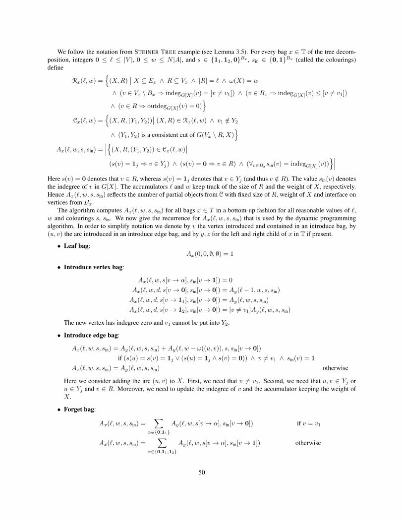
We follow the notation from STEINER TREE example (see Lemma 3.5). For every bag x ∈ T of the tree decom-position, integers 0 ≤ ` ≤ |V |, 0 ≤ w ≤ N |A|, and s ∈ 11,12,0Bx , sin ∈ 0,1Bx (called the colourings)define
Rx(`, w) =
(X,R)∣∣ X ⊆ Ex ∧ R ⊆ Vx ∧ |R| = ` ∧ ω(X) = w
∧ (v ∈ Vx \Bx ⇒ indegG[X](v) = [v 6= v1]) ∧ (v ∈ Bx ⇒ indegG[X](v) ≤ [v 6= v1])
∧ (v ∈ R⇒ outdegG[X](v) = 0)
Cx(`, w) =
(X,R, (Y1, Y2))∣∣ (X,R) ∈ Rx(`, w) ∧ v1 /∈ Y2
∧ (Y1, Y2) is a consistent cut of G(Vx \R,X)
Ax(`, w, s, sin) =∣∣∣(X,R, (Y1, Y2)) ∈ Cx(`, w)
∣∣(s(v) = 1j ⇒ v ∈ Yj) ∧ (s(v) = 0⇒ v ∈ R) ∧ (∀v∈Bxsin(v) = indegG[X](v))
∣∣∣Here s(v) = 0 denotes that v ∈ R, whereas s(v) = 1j denotes that v ∈ Yj (and thus v /∈ R). The value sin(v) denotesthe indegree of v in G[X]. The accumulators ` and w keep track of the size of R and the weight of X , respectively.Hence Ax(`, w, s, sin) reflects the number of partial objects from C with fixed size of R, weight of X and interface onvertices from Bx.
The algorithm computes Ax(`, w, s, sin) for all bags x ∈ T in a bottom-up fashion for all reasonable values of `,w and colourings s, sin. We now give the recurrence for Ax(`, w, s, sin) that is used by the dynamic programmingalgorithm. In order to simplify notation we denote by v the vertex introduced and contained in an introduce bag, by(u, v) the arc introduced in an introduce edge bag, and by y, z for the left and right child of x in T if present.
• Leaf bag:Ax(0, 0, ∅, ∅) = 1
• Introduce vertex bag:
Ax(`, w, s[v → α], sin[v → 1]) = 0
Ax(`, w, d, s[v → 0], sin[v → 0]) = Ay(`− 1, w, s, sin)
Ax(`, w, d, s[v → 11], sin[v → 0]) = Ay(`, w, s, sin)
Ax(`, w, d, s[v → 12], sin[v → 0]) = [v 6= v1]Ay(`, w, s, sin)
The new vertex has indegree zero and v1 cannot be put into Y2.
• Introduce edge bag:
Ax(`, w, s, sin) = Ay(`, w, s, sin) +Ay(`, w − ω((u, v)), s, sin[v → 0])
if (s(u) = s(v) = 1j ∨ (s(u) = 1j ∧ s(v) = 0)) ∧ v 6= v1 ∧ sin(v) = 1
Ax(`, w, s, sin) = Ay(`, w, s, sin) otherwise
Here we consider adding the arc (u, v) to X . First, we need that v 6= v1. Second, we need that u, v ∈ Yj oru ∈ Yj and v ∈ R. Moreover, we need to update the indegree of v and the accumulator keeping the weight ofX .
• Forget bag:
Ax(`, w, s, sin) =∑
α∈0,11Ay(`, w, s[v → α], sin[v → 0]) if v = v1
Ax(`, w, s, sin) =∑
α∈0,11,12Ay(`, w, s[v → α], sin[v → 1]) otherwise
50

If we forget v = v1, we require that its indegree is zero and v /∈ Y2. Otherwise, we require that the indegree ofthe forgotten vertex is one.
• Join bag: Let us define for T ⊆ Bx a colouring sin[T ] as sin[T ](v) = 1 if v ∈ T and sin[T ](v) = 0 otherwise.Then
Ax(`, w, s, sin) =∑
`1+`2=`+|s−1(0)|
∑w1+w2=w
∑T1,T2⊆Bx
[T1 ∪ T2 = s−1in (1)][T1 ∩ T2 = ∅]Ay(`1, w1, s, sin[T1])Az(`2, w2, s, sin[T2])
The colourings s in children need to be the same, whereas the colourings sin in the children need to sum up tothe colouring sin in the bag x, i.e., a vertex v has indegree one only if it has indegree one in exactly one of thechildren bags. Since vertices coloured 0 in Bx are accounted for in both tables of the children, we add theircontribution to the accumulator `.
To compute the recursion formula efficiently we need to use fast subset convolution. For accumulators `, w anda colouring s we define the following functions on subsets Bx
f `,w,s(T ) = Ay(`, w, s, sin[T ]),
g`,w,s(T ) = Az(`, w, s, sin[T ]).
Now note that
Ax(`, w, s, sin) =∑
`1+`2=`+|s−1(0)|
∑w1+w2=w
(f `1,w1,s ∗ g`2,w2,s)(s−1in (1))
By Theorem A.2, for fixed accumulators `1, w1, `2, w2 and a colouring s the term
(f `1,w1,s ∗ g`2,w2,s)(s−1in (1))
can be computed in time 2ttO(1) at once for all colourings sin. Thus, the total time consumed by the evaluationof Ax is bounded by 6tnO(1).
It is easy to see that the above recurrence leads to a dynamic programming algorithm that computes the parity of |C`W |for all values of W and ` in 6t|V |O(1) time, since |C`W | = Ar(`,W, ∅, ∅). Moreover, as we count the parities and notthe numbersAx themselves, all arithmetical operations (in particular the ring operations in the fast subset convolution)can be done in constant time. As discussed before, knowing in Z2 the values of |C`W | for 0 ≤ ` ≤ |V | − 1 we cancompute all values of |CkW | and |SkW | modulo 2. Thus, the proof of Theorem A.17 is finished.
A.6 MAXIMUM FULL DEGREE SPANNING TREE
In this subsection we solve a bit more general version of MAXIMUM FULL DEGREE SPANNING TREE where the treein question needs to contain exactly the prescribed number of vertices of full degree.
EXACT FULL DEGREE SPANNING TREEInput: An undirected graph G = (V,E) and an integer k.Question: Does there exist a spanning tree T of G for which there are exactly k vertices satisfying degG(v) =degT (v)?
Theorem A.18. There exists a Monte-Carlo algorithm that given a tree decomposition of width t solves the EXACTFULL DEGREE SPANNING TREE problem in 4t|V |O(1) time. The algorithm cannot give false positives and may givefalse negatives with probability at most 1/2.
51

Proof. We use the Cut&Count technique. As a universe we take the set of edges U = E. As usual we assume that weare given a weight function ω : U → 1, ..., N, where N = 2|U | = 2|E|. Let v1 be an arbitrary vertex.The Cut part. For an integer W we define:
1. RW to be the family of solution candidates of weight W , that is subsets of exactly |V | − 1 edges X ⊆ E,|X| = |V | − 1, ω(X) = W , such that there are exactly k vertices v satisfying degG(v) = degG[X](v),
2. SW to be the set of solutions, that is solution candidates X ∈ RW such that the graph G[X] is connected;
3. CW to be the family of pairs (X, (X1, X2)), where X ∈ RW , v1 ∈ X1, and (X1, X2) is a consistent cut of thegraph G[X].
Observe that for X ∈ RW the graph G[X] is connected iff G[X] is a tree, since |X| = |V | − 1. Thus SW is indeed afamily of solutions of weight W .The Count part. To use Algorithm 1 we need to formally prove that for any W we have |SW | ≡ |CW |. Similarly asin the case of STEINER TREE we note that by Lemma 3.3 for each X ∈ RW there exist 2cc(G[X])−1 consistent cuts ofthe graph G[X], and the claim follows.
To finish the proof we need to show how to compute |CW |modulo 2 in time 4tnO(1) using dynamic programming.In a state we store the number of vertices that are already forgotten and have all their incident edges chosen, thenumber of already chosen edges, the sum of weights of already chosen edges, and moreover for each vertex of the bagwe remember the side of the cut and one bit of information whether there exists some already introduced edge incidentwith that vertex that was not chosen. Formal definition follows.
We follow the notation from STEINER TREE example (see Lemma 3.5). For a bag x ∈ T of the tree decomposition,integers 0 ≤ i ≤ |V |, 0 ≤ b < |V |, 0 ≤ w ≤ N(|V |−1), scut ∈ 1,2Bx and sdeg ∈ 0,1Bx (called the colouring)define
Rx(i, b, w) =X ⊆ Ex
∣∣ |X| = b ∧ ω(X) = w ∧ |v ∈ Vx \Bx : degGx(v) = degX(v)| = i
Cx(i, b, w) =
(X, (X1, X2))∣∣ X ∈ Rx(i, b, w) ∧ v1 ∈ X1 ∧ (X1, X2) is a consistent cut of (Vx, X)
Ax(i, b, w, scut, sdeg) =
∣∣∣(X, (X1, X2)) ∈ Cx(i, b, w)∣∣(v ∈ Xj ∩Bx ⇒ scut(v) = j)
∧ (sdeg(v) = 0⇒ degGx(v) = degX(v)) ∧ (sdeg(v) = 1⇒ degGx(v) > degX(v))∣∣∣
By scut(v) = j we denote v ∈ Xj , whereas sdeg(v) is equal to one iff there exists an edge in Ex \ X that isincident with v. Hence Ax(i, b, w, scut, sdeg) is the number of pairs from Cx(i, b, w) with a fixed interface on verticesfrom Bx.
The algorithm computes Ax(i, b, w, scut, sdeg) for all bags x ∈ T in a bottom-up fashion for all reasonable valuesof i, b, w, scut and sdeg. We now give the recurrence for Ax(i, b, w, scut, sdeg) that is used by the dynamic program-ming algorithm. As usual v denotes the vertex introduced and contained in an introduce bag, uv the edge introducedin an introduce edge bag, and y, z the left and right child of x in T if present.
• Leaf bag:Ax(0, 0, 0, ∅, ∅) = 1
• Introduce vertex bag:
Ax(i, b, w, scut[v → 1], sdeg[v → 0]) = Ay(i, b, w, scut, sdeg)
Ax(i, b, w, scut[v → 2], sdeg[v → 0]) = [v 6= v1]Ay(i, b, w, scut, sdeg)
Ax(i, b, w, scut[v → α], sdeg[v → 1]) = 0
We make sure that v1 belongs to X1.
52

• Introduce edge bag:
Ax(i, b, w, scut, sdeg) = [scut(u) = scut(v)]Ay(i, b− 1, w − ω(uv), scut, sdeg)
+∑
αu,αv∈0,1Ay(i, b, w, scut, sdeg[u→ αu, v → αv])
if sdeg(u) = sdeg(v) = 1
Ax(i, b, w, scut, sdeg) = [scut(u) = scut(v)]Ay(i, b− 1, w − ω(uv), scut, sdeg)
otherwise
If sdeg(u) = sdeg(v) = 1 then we have an option of not taking the edge uv to the set X . In this case, theprevious values of sdeg(u) and sdeg(v) can be arbitrary.
• Forget bag:
Ax(i, b, w, scut, sdeg) =∑
j∈1,2
∑α∈0,1
Ay(i− [α = 0], b, w, scut[v → j], sdeg[v → α])
If the vertex v had all incident edges chosen (α = 0) then we update the accumulator i.
• Join bag:
The only valid combinations to achieve the colouring scut is to have the same colouring in both children. How-ever we have sdeg(v) = 1 in x if and only if sdeg(v) = 1 in y or in z. Hence we use a covering product. Wesomewhat abuse the notation and identify a function sdeg with a subset s−1
deg(1) ⊆ Bx. Let us define
f i,b,w,scut(sdeg) = Ay(i, b, w, scut, sdeg)
gi,b,w,scut(sdeg) = Az(i, b, w, scut, sdeg)
hi,b,w,scut(sdeg) =∑
i1+i2=i
∑b1+b2=b
∑w1+w2=w
(f i1,b1,w1,scut ∗c gi2,b2,w2,scut)(sdeg)
Consequently we have
Ax(i, b, w, scut, sdeg) = hi,b,w,scut(sdeg)
It is easy to see that we can combine the above recurrence with dynamic programming. For each of the 2t|V |O(1)
argument values of i,b,w and scut the covering product ∗c can be computed in 2t|V |O(1) by Theorem A.2. Note thatas we perform all calculations modulo 2, we take only constant time to perform any arithmetic operation.
Since |CW | = Ar(k, |V | − 1,W, ∅, ∅) the above recurrence leads to a dynamic programming algorithm that com-putes the parity of |CW | (and thus of |SW | as well) for all reasonable values of W in 4t|V |O(1) time. Consequently wefinish the proof of Theorem A.18.
A.7 GRAPH METRIC TRAVELLING SALESMAN PROBLEM
GRAPH METRIC TRAVELLING SALESMAN PROBLEMInput: An undirected graph G = (V,E) and an integer k.Question: Does there exist a closed walk (possibly repeating edges and vertices) of length at most k that visits eachvertex of the graph at least once?
Theorem A.19. There exists a Monte-Carlo algorithm that given a tree decomposition of width t solves the GRAPHMETRIC TRAVELLING SALESMAN PROBLEM problem in 4t|V |O(1) time. The algorithm cannot give false positivesand may give false negatives with probability at most 1/2.
53

Proof. We use the Cut&Count technique. Observe that we may assume that G is connected and k ≤ 2(|V | − 1)because taking twice all edges of any spanning tree gives a solution.
Since we want to distinguish the case when we take an edge once or twice to the solution, as a universe we takethe set U = E × 1, 2, where we use (e, 1) if an edge is chosen once and (e, 2) in case we use e twice. As usualwe assume that we are given a weight function ω : U → 1, ..., N, where N = 2|U | = 4|E|. Let v1 be an arbitraryvertex.The Cut part. For integers i and W we define:
1. RiW to be the family of solution candidates of size i and weight W , that is functions φ ∈ 0, 1, 2E where∑e∈E φ(e) = i,
∑e∈E,φ(e)>0 ω((e, φ(e))) = W , such that for each vertex v ∈ V its degree is even, i.e.,
|uv ∈ E : φ(e) = 1| ≡ 0;
2. SiW to be the set of solutions, that is solution candidates φ ∈ RiW such that the graph G[φ−1(1, 2)] is con-nected;
3. CiW to be the family of pairs (φ, (X1, X2)), where φ ∈ RiW , v1 ∈ X1, and (X1, X2) is a consistent cut of thegraph G[φ−1(1, 2)].
We want to check whether there exist numbers W and i ≤ k such that SiW 6= ∅.The Count part. To use Algorithm 1 we need to formally prove that for any i andW we have |SiW | ≡ |CiW |. Similarlyas in the case of STEINER TREE we note that by Lemma 3.3 for each φ ∈ RiW there exist 2cc(G
′)−1 consistent cuts ofthe graph G′ = G[φ−1(1, 2)], and the claim follows.
To finish the proof we need to show how to compute |CiW |modulo 2 in time 4tnO(1) using dynamic programming.We follow the notation from STEINER TREE example (see Lemma 3.5). For a bag x ∈ T of the tree decomposition,
integers 0 ≤ i ≤ k, 0 ≤ w ≤ kN , scut ∈ 1,2Bx and sdeg ∈ 0,1Bx (called the colourings) define
Rx(i, w) =φ ∈ 0, 1, 2Ex
∣∣ ∑e∈Ex
φ(e) = i ∧∑
e∈Ex,φ(e)>0
ω((e, φ(e))) = w
∧ ∀v∈Vx\Bx |uv ∈ Ex : φ(uv) = 1| mod 2 = 0
Cx(i, w) =
(φ, (X1, X2))∣∣ φ ∈ Rx(i, w) ∧ v1 ∈ X1 ∧ (X1, X2) is a consistent cut of Gx[φ−1(1, 2)]
Ax(i, w, scut, sdeg) =
∣∣∣(φ, (X1, X2)) ∈ Cx(i, w)∣∣(scut(v) = j ⇒ v ∈ Xj)
∧ ∀v∈Bxsdeg(v) ≡ |uv ∈ Ex : φ(uv) = 1|∣∣∣
The accumulators i and w keep track of the number of edges chosen (with multiplicities) and the appropriate sumof weights. In the sequence scut we store the information about the side of the cut of each vertex from Bx, whereassdeg is used to remember whether a vertex has an odd or even degree. Hence Ax(i, w, scut, sdeg) is the number ofpairs from Cx(i, w) with a fixed interface on vertices from Bx.
The algorithm computes Ax(i, w, scut, sdeg) for all bags x ∈ T in a bottom-up fashion for all reasonable valuesof i, w, scut and sdeg. We now give the recurrence for Ax(i, w, scut, sdeg) that is used by the dynamic programmingalgorithm. As usual let v stand for the vertex introduced and contained in an introduce bag, uv for the edge introducedin an introduce edge bag, and y, z for the left and right child of x in T if present.
• Leaf bag:Ax(0, 0, ∅, ∅) = 1
• Introduce vertex bag:
Ax(i, w, scut[v → 1], sdeg[v → 0]) = Ay(i, w, scut, sdeg)
Ax(i, w, scut[v → 2], sdeg[v → 0]) = [v 6= v1]Ay(i, w, scut, sdeg)
Ax(i, w, scut[v → α], sdeg[v → 1]) = 0
We make sure that v1 belongs to X1.
54

• Introduce edge bag:
Ax(i, w, scut, sdeg) = Ay(i, w, scut, sdeg)+
[scut(u) = scut(v)]Ay(i− 1, w − ω((uv, 1)), scut, s′deg)+
[scut(u) = scut(v)]Ay(i− 2, w − ω((uv, 2)), scut, sdeg)
where by s′deg we denote sdeg with changed values for u and v, formally
s′deg = sdeg[u→ 1− sdeg(u), v → 1− sdeg(v)].
We can either not take an edge or take it once or twice.
• Forget bag:
Ax(i, w, scut, sdeg) =∑
j∈1,2Ay(i, w, scut[v → j], sdeg[v → 0])
We simply check the parity of the vertex which we are about to forget, both sides of the cut are allowed.
• Join bag:
The only valid combinations to achieve the colouring scut is to have the same colouring in both children. How-ever for sdeg we have to calculate the xor product of sdeg(v) for y and z. We somewhat abuse the notation andidentify a function sdeg with a subset s−1
deg(1) ⊆ Bx. Let us define
f i,w,scut(sdeg) = Ay(i, w, scut, sdeg)
gi,w,scut(sdeg) = Az(i, w, scut, sdeg)
hi,w,scut(sdeg) =∑
i1+i2=i
∑w1+w2=w
(f i1,w1,scut ∗x gi2,w2,scut)(sdeg)
Consequently we have
Ax(i, w, scut, sdeg) = hi,w,scut(sdeg)
It is easy to see that we can combine the above recurrence with dynamic programming. For each of the 2t|V |O(1)
argument values of i,w and scut the xor product can be computed in 2t|V |O(1) by Theorem A.6. Note that as weperform all calculations modulo 2, we take only constant time to perform any arithmetic operation.
Since for each i we have |CiW | = Ar(i,W, ∅, ∅) the above recurrence leads to a dynamic programming algorithmthat computes the parity of |CiW | (and thus of |SiW | as well) for all reasonable values of W and i in 4t|V |O(1) time.Consequently we finish the proof of Theorem A.19.
B Improvements in FVS, CVC and CFVS parameterized by the solutionsize
Our technique gives rise to an improvement of several parameterized complexity upper bounds for vertex deletionproblems in which the remaining graph has to be of constant treewidth. These problems are FEEDBACK VERTEXSET, CONNECTED VERTEX COVER and CONNECTED FEEDBACK VERTEX SET. The main idea behind the newresults is the combination of the iterative compression technique, developed by Reed et al. [55], and the Cut&Counttechnique.
We begin with the FEEDBACK VERTEX SET problem, as it was exhaustively studied by the parameterized com-plexity community. Let us recall that previously best algorithm, due Cao, Chen and Liu, runs in 3.83knO(1) time[14].
55

Theorem B.1 (Theorem 1.6, restated). There exists a Monte-Carlo algorithm for the FEEDBACK VERTEX SET prob-lem in a graph with n vertices in 3knO(1) time and polynomial space. The algorithm cannot give false positives andmay give false negatives with probability at most 1/2.
Proof. Let v1, v2, . . . , vn be an arbitrary ordering of the vertices of the given graph G = (V,E). Let us denoteGi = G[v1, v2, . . . , vi] for all 1 ≤ i ≤ n. Observe that if G admits a feedback vertex set of size at most k, i.e. thereis a set A ⊆ V, |A| ≤ k such that G[V \ A] is a forest, then so do all the graphs Gi, because Gi[v1, v2, . . . , vi \ A]is a forest as well and |A ∩ v1, v2, . . . , vi| ≤ |A| ≤ k.
We construct feedback vertex sets A1, A2, . . . , An of size at most k consecutively in G1, G2, . . . , Gn = G. Ifat any step the algorithm finds out that the set we seek does not exist (with high probability), we answer NO. Webegin with A1 = ∅, which is a feasible solution in graph G1 (we ignore the trivial case k = 0). The idea of iterativecompression is that when we are to construct the set Ai+1, we can use the previously constructed set Ai. Let Bi+1 =Ai ∪vi+1. Observe that Bi+1 is a feedback vertex set in Gi+1. If |Bi+1| ≤ k, then we take Ai+1 = Bi+1. Thus weare left with the case in which, given a feedback vertex set of size k+ 1, we need to construct a feedback vertex set ofsize at most k or determine that none such exists. Denote this given feedback vertex set by B.
As B is a feedback vertex set, the graph induced by the rest of the vertices is a forest. Thus we can constructa tree decomposition of the graph Gi+1 of width at most k + 2 by creating a tree decomposition of the forest ofwidth 1 and adding the whole set B to each bag. To begin with, we test whether Gi+1 admits a feedback vertex setof size at most k. We apply (using the tree decomposition obtained above as the input) the dynamic programmingalgorithm described in Section A.2, running in 3knO(1) time, which tests whether the graph admits a feedback vertexset of size at most k. Observe that this algorithm, as described in the proof of Theorem A.8, uses exponential space.However, in each step when computingAx(a, b, c, w, s) the algorithm refers only to valuesAy(a′, b′, c′, w′, s′), wheres′ = s on the intersection of the domains of s and s′. In our case the intersection of every two bags of the treedecomposition contains B. Therefore we can reorder the computation in the following manner: for every evaluations : B → 0,11,12 we fix it as the ,,core” evaluation for every bag in the decomposition and run the algorithm tocompute all the values Ax(a, b, c, w, s), where s|B = s. Such a computation takes polynomial time and space. Asthere are 3k+1 such possible evaluations s, the algorithm runs in 3knO(1) time and in polynomial space. We make nindependent runs of the algorithm in order to assure that the probability of a false negative is at most 1
2n .Once we have done this, we already tested with high probability whether the desired feedback vertex set exists or
not. If the answer is negative, we answer NO. Otherwise we need to explicitly construct the set Ai+1 in order to use itin the next step of the iterative compression. We make use of the algorithm for CONSTRAINED FEEDBACK VERTEXSET, given by Theorem A.8. The algorithm considers the vertices of Gi+1 one by one, building a set K which at theend will be the constructed Ai+1. We begin with K = ∅ and preserve an invariant that at each step there is a feedbackvertex set of size at most k containing the set K. When considering the vertex v, we test in 3knO(1) time whether thegraph admits a constrained feedback vertex set of size at most k with S = K ∪v, making n independent runs of thealgorithm given by Theorem A.8 in order to reduce the probability of a false negative to at most 1
2n . If the answer ispositive, we can safely add v to K as we know that there is a feedback vertex set of size at most k containing K ∪ v(recall our algorithms do not return false positives). Otherwise we simply proceed to the next vertex. The computationterminates when K is already a feedback vertex set or when we have exhausted all vertices. Observe that if Gi+1
admits a feedback vertex set of size at most k, this construction will terminate building a feedback vertex set Ai+1 ofsize at most k unless there was an error in at least one of the tests. If we exhaust all vertices, we answer NO, as anerror has occured. Note that in each run of the algorithm for CONSTRAINED FEEDBACK VERTEX SET we can reorderthe computation in the same way as in the previous paragraph to reduce space usage to polynomial.
Observe that the described algorithm at most n2 + n times makes n independent runs of the algorithm fromTheorem A.8 as a subroutine: in each of n steps of the iterative compression at most n+1 times. Each of these groupsof runs has a probability of a false negative bounded by 1
2n , thus the probability of a false negative is bounded byn2+n
2n , which is lower than 12 for large enough n.
Now we proceed to the algorithm for CONNECTED VERTEX COVER. The previously best FPT algorithm is dueto Binkele-Raible [5], and runs in 2.4882knO(1) time complexity. The following algorithm is also an application ofiterative compression, however we make use of the connectivity requirement in order to reduce the complexity from3knO(1) down to 2knO(1).
56
Theorem B.2. There exists a Monte-Carlo algorithm for the CONNECTED VERTEX COVER problem in a graph with nvertices in 2knO(1) time and polynomial space. The algorithm cannot give false positives and may give false negativeswith probability at most 1/2.
Proof. Firstly observe that CONNECTED VERTEX COVER problem is contraction–closed. This means that if a graphH admits a connected vertex cover A of size at most k, then H ′ obtained from H by contracting an edge of H (andreducing possible multiedges to simple edges) also admits a connected vertex cover A′ of size at most k. Indeed, thecontracted edge uv needs to be covered by A, so u ∈ A or v ∈ A. Thus we can construct A′ by removing u and vfrom A and adding the vertex obtained from the contracted edge. It can be easily seen that A′ is a connected vertexcover of H ′ of size at most k.
Therefore, we can consider a sequence of graphs G1, G2, . . . , Gn = G (G is the connected graph given in theinput), where Gi is obtained from Gi+1 by contracting any edge and reducing possible multiedges to simple edges,and G1 is a graph composed of a single vertex. The argument from the last paragraph ensures that we can proceedas in the proof of Theorem B.1, namely construct connected vertex covers for G1, G2, . . . , Gn consecutively, and theonly thing we have to to show is how to construct a connected vertex cover of size k in Gi+1 given a connected vertexcover Ai of size k in Gi, or determine that none exists.
Let Gi be constructed from Gi+1 by contracting an edge uv. We construct B from Ai by removing the vertexobtained in the contraction (if it was contained in Ai) and inserting both u and v. Observe that B is of size atmost k + 2 and it is a vertex cover of Gi+1. As V (Gi+1) \ B is an independent set, then we can construct a pathdecomposition of Gi+1 of width at most k + 2: for every vertex from V (Gi+1) \ B we introduce a bag, connect thebags in any order and then add the set B to every bag.
Now we are going to test whether Gi+1 admits a connected vertex cover of size at most k. We could applythe algorithm from Theorem A.10. As in the proof of Theorem B.1, this dynamic programming algorithm duringcomputation ofAx(i, w, s) also refers only to valuesAy(i′, w′, s′) for s′ such that s = s′ on the intersection of domainsof s and s′. Therefore, similarly as before, we would iterate through all possible evaluations s : B → 0,11,12,each time computing all the values Ax(i,W, s) such that s|B = s in polynomial time, thus using only polynomialspace in the whole algorithm. Unfortunately, the algorithm given by Theorem A.10 runs in 3knO(1) time.
We can, however, reduce the complexity by bounding the number of reasonable evaluations s : B → 0,11,12by 33 ·2k−1. B induces in Gi+1 a graph with consisting of a single large connected component (coming from Ai), andat most two additional vertices. Take any spanning tree of the large component and root it at some vertex r. We presentthe evaluation s in the following manner. For the root r and the two additional vertices we choose for s any value from0,11,12, giving 33 choices in total. Now consider the rest of the tree (containing all the remaining vertices fromB) in a top–down manner. Observe that every vertex v from the tree has only two possible evaluation, depending onthe evaluation of its parent u:
• if s(u) = 0, the two possible options are 11,12, as otherwise the edge connecting v with its parent would notbe covered;
• if s(u) = 1j , the two possible options are 0 and 1j , as otherwise the evaluation s would not describe anyconsistent cut.
Thus each of k + 2 elements of B has only two options, except from the starting 3, which have 3 options each. Thismeans we only need to consider 33 · 2k−1 possible ,,core” evaluations s, which yields an algorithm with running time2knO(1), using polynomial space. As previously, we make n independent runs of the algorithm in order to reduce theprobability of a false negative to at most 1
2n .Once we have tested whetherGi+1 admits a connected vertex cover of size at most k, we can construct it explicitly
similarly as in the proof of Theorem B.1 using the algorithm for CONSTRAINED CONNECTED VERTEX COVER. Weconsider vertices one by one, each time determining whether the vertex can be inserted into the constructed connectedvertex cover by running the algorithm from Theorem A.10 n times. Observe that all these runs can be done in 2knO(1)
time and polynomial space complexity using the same technique as in the testing. Thus we succeed in constructingAi+1 unless at least one of the tests returns a false negative.
The algorithm makes at most n2 + n groups of n independent runs of algorithm from Theorem A.10. Thereforethe probability of a false negative is bounded by n2+n
2n which is less than 12 for large enough n.
57
Finally, we use a similar technique to obtain an algorithm for CONNECTED FEEDBACK VERTEX SET. The previ-ously best FPT algorithm is due to Misra et al. [49], and runs in 46.2knO(1) time complexity.
Theorem B.3. There exists a Monte-Carlo algorithm solving the CONNECTED FEEDBACK VERTEX SET problem ina graph with n vertices in 3knO(1) time and polynomial space. The algorithm cannot give false positives and may givefalse negatives with probability at most 1/2.
Proof. Similarly as in the proof of Theorem B.2, the CONNECTED FEEDBACK VERTEX SET problem is also contrac-tion–closed. Consider any graph H and obtain H ′ by contracting an edge uv into a vertex w. Consider a connectedfeedback vertex set A of a graph H of size at most k and construct a set A′ ⊆ V (H ′) as following:
• if u, v /∈ A then A′ = A;
• otherwise A′ = (A ∪ w) \ u, v.It can be easily seen that A′ is a connected feedback vertex set of H ′ of size at most k.
This observation enables us to use iterative compression approach, similarly as in the proof of Theorem B.2.Namely we consider a sequence of graphs G1, G2, . . . , Gn = G (G is the connected graph given in the input), whereGi is obtained from Gi+1 by contracting any edge and reducing possible multiedges to simple edges. For every Gi wetry to construct a connected feedback vertex set Ai in a consecutive manner and if at any step we fail, we can safelyanswer NO. Thus we need to show a way of constructing a connected feedback vertex set of size k in Gi+1 given aconnected feedback vertex set Ai of size k in Gi, or determining that none exists.
Let Gi be constructed from Gi+1 by contracting an edge uv. We construct B from Ai by removing the vertexobtained in the contraction (if it was included in Ai) and inserting both u and v. Observe that B is a feedback vertexset ofGi+1 of size at most k+2 containing a connected component of size at least |B|−2. Therefore, we can constructa tree decomposition of graph Gi+1 of width k + 3 by constructing the tree decomposition of width 1 of the forestGi+1 \B and including B into every bag.
Now we are going to test whether Gi+1 admits a connected feedback vertex set of size at most k. A straight-forward application of the algorithm from Theorem A.13 would yield an algorithm with running time 4knO(1). Thisalgorithm once again has the property of referring only to previously computed values with the same evaluation onthe intersection of the domains, so we can also apply the method already used in proofs of Theorems B.1 and B.2 toreduce the space usage to polynomial.
Once again, using the special structure of the set B we can also reduce the time complexity down to 3knO(1) bybounding the number of reasonable evaluations s : B → 01,02,11,12 by 433k−1. B is a graph consisting of a largeconnected component and at most two additional vertices. Take any spanning tree of the connected component androot it in a vertex r. Each reasonable evaluation s can be coded in the following manner: vertex r and the two possibleadditional vertices have 4 possibilities of the value in s, but every other vertex in the tree has only three possibilities,depending on the value s(u), where u denotes the parent of v:
• if s(u) = 0j , the possibilities are 11, 12 and 0j ;
• if s(u) = 1j , the possibilities are 01, 02 and 1j ;
as otherwise the cut could not be consistent. Thus every vertex from B has only 3 possibilities, apart from at most 3,which have 4 possibilities. So the number of reasonable evaluations s is bounded by 433k−1, thus the testing algorithmruns in time complexity 3knO(1) and uses polynomial space. Again we make n independent runs of the algorithm inorder to reduce the probability of a false negative to at most 1
2n .The idea of reconstructing the solution is the same as in the proofs of Theorems B.1 and B.2. We consider
vertices one by one iteratively constructing a connected feedback vertex set. At each step we determine whether theconsidered vertex can or cannot be taken as the next vertex of the so far built part of the solution, using the algorithmfor CONSTRAINED CONNECTED FEEDBACK VERTEX SET obtained in Theorem A.13. If it can, we take it, otherwisewe just proceed to the next vertex. At each step we make n independent runs to reduce the probability of a falsenegative to at most 1
2n . If the graph admitted a connected feedback vertex set of size at most k, we will construct it inthis manner unless at least one test gives a false negative. Again, using previous observations the computation in eachof the runs can be reordered so that the running time is 3knO(1) and the space usage is polynomial.
58

Again, the union bound proves that the probability of obtaining a false negative in any of the tests is bounded byn2+n
2n which for large enough n is lower than 12 , as we make at most n2 + n groups of n independent runs of the
algorithm from Theorem A.13.
C Negative results under ETHIn this section we provide an evidence that the problems, where we want not to minimize, but to maximize thenumber of connected components, are harder, in the sense, that they probably do not admit algorithms running intime 2o(p log p)nO(1), where p denotes the pathwidth of the input graph. More precisely, we show that assumingETH there do not exist algorithms for CYCLE PACKING, MAX CYCLE COVER and MAXIMALLY DISCONNECTEDDOMINATING SET running in time 2o(p log p)nO(1).
Let us recall formal problem definitions. The first two problems have undirected and directed versions.
CYCLE PACKINGInput: A (directed or undirected) graph G = (V,E) and an integer `Question: Does G contain ` vertex-disjoint cycles?
MAX CYCLE COVERInput: A (directed or undirected) graph G = (V,E) and an integer `Question: Does G contain a set of at least ` vertex-disjoint cycles such that each vertex of G is contained in exactlyone cycle?
MAXIMALLY DISCONNECTED DOMINATING SETInput: An undirected graph G = (V,E) and integers ` and rQuestion: Does G contain a dominating set of size at most ` that induces at least r connected components?
We prove the following theorem.
Theorem C.1 (Theorem 5.1 restated). Assuming ETH, there is no 2o(p log p)nO(1) time algorithm for CYCLE PACK-ING, MAX CYCLE COVER (both in the directed and undirected setting) nor for MAXIMALLY DISCONNECTED DOM-INATING SET. The parameter p denotes the width of a given path decomposition of the input graph.
We start our reductions from k × k HITTING SET and k × k PERMUTATION HITTING SET problems. As wediscussed in Section 5.1, the non-permutation version was introduced and analyzed by Lokshtanov et al. [48]. Wedenote [k] = 1, 2, . . . , k. In the set [k]× [k] a row is a set i× [k] and a column is a set [k]×i (for some i ∈ [k]).We include formal definitions for sake of completeness.
k × k HITTING SETInput: A family of sets S1, S2 . . . Sm ⊆ [k] × [k], such that each set contains at most one element from each row of[k]× [k].Question: Is there a set S containing exactly one element from each row such that S ∩ Si 6= ∅ for any 1 ≤ i ≤ m?
k × k PERMUTATION HITTING SETInput: A family of sets S1, S2 . . . Sm ⊆ [k] × [k], such that each set contains at most one element from each row of[k]× [k].Question: Is there a set S containing exactly one element from each row and exactly one element from each columnsuch that S ∩ Si 6= ∅ for any 1 ≤ i ≤ m?
Theorem C.2 ([48], Theorem 2.4). Assuming ETH, there is no 2o(k log k)nO(1) time algorithm for k×k HITTING SETnor for k × k PERMUTATION HITTING SET.
Note that in [48] the statement of the above theorem only includes k × k HITTING SET. However, the proof in[48] works for the permutation variant as well without any modifications.
59

We first prove the bound for MAXIMALLY DISCONNECTED DOMINATING SET by quite simple reduction fromk × k HITTING SET. This is done in Section C.1. Then, in Section C.2 we prove the bound for undirected CYCLEPACKING, by quite involved reduction from k×k PERMUTATION HITTING SET. In Section C.3 we provide a reductionto directed CYCLE PACKING and in Section C.4 we provide a reduction to MAX CYCLE COVER in both variants.
C.1 MAXIMALLY DISCONNECTED DOMINATING SET
In this subsection we provide a reduction from k × k HITTING SET to MAXIMALLY DISCONNECTED DOMINATINGSET. We are given an instance (k, S1, . . . , Sm) of k × k HITTING SET, called the initial instance, and we are toconstruct an equivalent instance (G, `, r) of MAXIMALLY DISCONNECTED DOMINATING SET.
We first set ` := 3k +m and r := k.
C.1.1 Gadgets
We introduce a few simple gadgets used repeatedly in the construction. In all definitions H = (V,E) is an undirectedgraph, and the parameters ` and r are fixed.
Definition C.3. By adding a force gadget for vertex v ∈ V we mean the following construction: we introduce ` + 1new vertices of degree one, connected to v.
Lemma C.4. If graph G is constructed from graph H = (V,E) by adding a force gadget to vertex v ∈ V , then v iscontained in each dominating set in G of size at most `.
Proof. If D is a dominating set in G, and v /∈ D, then all new vertices added in the force gadget need to be includedin D. Thus |D| ≥ `+ 1.
Definition C.5. By adding a one-in-many gadget to vertex set X ⊆ V we mean the following construction: weintroducte `+ 1 new vertices of degree |X|, connected to all vertices in X .
Lemma C.6. If graphG is constructed from graphH = (V,E) by adding a one-in-many gadget to vertex setX ⊆ V ,then each dominating set in G of size at most ` contains a vertex from X .
Proof. If D is a dominating set in G, and X ∩D = ∅, then all new vertices added in the one-in-many gadget need tobe included in D. Thus |D| ≥ `+ 1.
We conclude with the pathwidth bound.
Lemma C.7. Let G be a graph and let G′ be a graph constructed from G by adding multiple force and one-in-manygadgets. Assume we are given a path decomposition ofG of width p with the following property: for each one-in-manygadget, attached to vertex set X , there exists a bag in the path decomposition that contains X . Then, in polynomialtime, we can construct a path decomposition of G′ of width at most p+ 1.
Proof. Let w be a vertex in G′, but not in G, i.e., a vertex added in one of the gadgets. By the assumptions of thelemma, there exists a bag Vw in the path decomposition ofG that containsN(w). For each such vertexw, we introducea new bag V ′w = Vw ∪ w and we insert it into the path decomposition after the bag Vw. If Vw is multiplied for manyvertices w, we insert all the new bags after Vw in an arbitrary order.
It is easy to see that the new path decomposition is a proper path decomposition of G′, as V ′w covers all edges inci-dent to w. Moreover, we increased the maximum size of bags by at most one, thus the width of the new decompositionis at most p+ 1.
60

C.1.2 Construction
Let Srowi = i× [k] be a set containing all elements in the i-th row in the set [k]× [k]. We denote S = Ss : 1 ≤ s ≤m ∪ Srowi : 1 ≤ i ≤ k. Note that for each A ∈ S we have |A| ≤ k, as each set Si contains at most one elementfrom each row.
First let us define the graph H . We start by introducing vertices pLi for 1 ≤ i ≤ k and vertices pRj for 1 ≤ j ≤ k.Then, for each set A ∈ S we introduce vertices xAi,j for all (i, j) ∈ A and edges pLi x
Ai,j and pRj x
Ai,j . Let XA = xAi,j :
(i, j) ∈ A.To construct graph G, we attach the following gadgets to graph H . For each 1 ≤ i ≤ k and 1 ≤ j ≤ k we attach
force gadgets to vertices pLi and pRj . Moreover, for each A ∈ S we attach one-in-many gadget to the set XA.We now provide a pathwidth bound on the graph G.
Lemma C.8. The pathwidth of G is at most 3k.
Proof. First consider the following path decomposition of H . For each A ∈ S we create a bag
VA = pLi : 1 ≤ i ≤ k ∪ pRj : 1 ≤ j ≤ k ∪ xAi,j : (i, j) ∈ A.
The path decomposition of H consists of all bags VA for A ∈ S in an arbitrary order. Note that the above pathdecomposition is a proper path decomposition of H of width at most 3k − 1 (as |A| ≤ k for each A ∈ S) and itsatisfies conditions for Lemma C.7.
C.1.3 From hitting set to dominating set
Lemma C.9. If the initial k × k HITTING SET instance was a YES-instance, then there exists a dominating set D inthe graph G, such that |D| = ` and D induces exactly r connected components.
Proof. Let S be a solution to the initial k × k HITTING SET instance (k, S1, . . . , Sm). For each A ∈ S fix an element(iA, jA) ∈ S ∩ A. Recall that S contains exactly one element from each row, thus S ∩ A 6= ∅ for all sets A ∈ S. Letus define:
D = pLi : 1 ≤ i ≤ k ∪ pRj : 1 ≤ j ≤ k ∪ xAiA,jA : A ∈ S.First note that |D| = 3k+m, as there are k vertices pLi , k vertices pRj , and |S| = k+m, since S consists of m sets
Ss and k sets Srowi .Let us now check whether D is a dominating set in G. Vertices pLi and pRj for 1 ≤ i, j ≤ k dominate all vertices
of the graph H and all vertices added in the attached force gadgets. Moreover, D ∩XA = xAiA,jA for each A ∈ S,thus D dominates all vertices added in one-in-many gadgets attached to sets XA.
We now prove that G[D] contains exactly r = k connected components. Let us define for each 1 ≤ j ≤ k:
Dj = pRj ∪ pLi : (i, j) ∈ S ∪ xAiA,jA : A ∈ S, jA = j.
Note that Dj is a partition of D into k pairwise disjoint sets. Moreover, observe that G[Dj ] is connected and, since Scontains exactly one element from each row, no vertices from Dj and Dj′ are adjacent, for j 6= j′. This finishes theproof of the lemma.
C.1.4 From dominating set to hitting set
Lemma C.10. If there exists a dominating setD in the graphG, such that |D| ≤ ` andD induces at least r connectedcomponents, then the initial k × k HITTING SET instance was a YES-instance.
Proof. By the properties of the force gadget, D needs to include all forced vertices, i.e., vertices pLi and pRj for1 ≤ i, j ≤ k. There are 2k forced vertices, thus we have `− 2k = k +m vertices left.
By the properties of one-in-many gadgets, D needs to include at least one vertex from each set XA, A ∈ S. But|S| = k + m and sets XA are pairwise disjoint. Thus, D consist of all forced vertices and exactly one vertex fromeach set XA, A ∈ S.
61

For each 1 ≤ i ≤ k let xSrowi
i,f(i) be the unique vertex in D ∩XSrowi . Let S = (i, f(i)) : 1 ≤ i ≤ k. We claim that
S is a solution to the initial k × k HITTING SET instance. It clearly contains exactly one element from each row.Let Dj be the vertex set of the connected component of G[D] that contains pRj . Note that pLi ∈ Dj whenever
j = f(i), i.e., (i, j) ∈ S. This implies that⋃kj=1Dj contains all vertices pLi . Moreover, as each vertex in XA for
A ∈ S is adjacent to some vertex pRj , the sets Dj are the only connected components of G[D]. As G[D] contains atleast r = k connected components, Dj 6= Dj′ for j 6= j′.
Let 1 ≤ s ≤ m and let us focus on set Ss ∈ S. Let xSsi,j be the unique vertex in D ∩XSs . Note that xSsi,j connectspLi ∈ Df(i) with pRj ∈ Dj . As sets Dj are pairwise distinct, this implies that j = f(i) and (i, j) ∈ S ∩ Ss. Thus thecomponents of G[D] are exactly the sets Dj , 1 ≤ j ≤ k.
C.2 Undirected CYCLE PACKING
C.2.1 Proof overview and preliminaries
First note that for CYCLE PACKING, we can assume that the input graph may be a multigraph, i.e., it may containmultiple edges and loops. The following lemma summarizes this observation.
Lemma C.11. Let (G, `) be an instance of (directed or undirected) CYCLE PACKING, where G may contain multipleedges and loops. Then we can construct in polynomial time an equivalent (directed or undirected, respectively)instance (G′, `), such that G′ does not contain multiple edges nor loops. Moreover, given a path decomposition of Gof width p, we can construct in polynomial time a path decomposition of G′ of width at most p+ 2.
Proof. To construct G′, we replace each edge e ∈ E(G) with a path of length three, i.e., we insert vertices u1e and u2
e
in the middle of edge e. Clearly G is a simple graph and vertex-disjoint cycle families in G and G′ naturally translatesinto each other.
We are left with the pathwidth bound. Assume we have a path decomposition of G of width p. For each edgee ∈ E(G) we fix a bag Ve that covers e. We introduce a new bag V ′e = Ve ∪ u1
e, u2e and insert V ′e near the bag Ve
in the path decomposition. It is easy to see that the new decomposition is a proper path decomposition of G′ and itswidth is at most p+ 2.
Let us introduce some extra notation. We say that a vertex is covered by a cycle (or a family of cycles) if the vertexbelongs to the cycle (or belongs to at least one cycle in the family). A graph is covered by a cycle family if every itsvertex is covered by the family. By (v1, . . . , vr) we denote a path (or a cycle) consisting of vertices v1, v2, . . . , vr inthis order.
We now present an overview of the proof of Theorem 5.1 for undirected CYCLE PACKING. We provide a construc-tion that, given an instance (k, S1, S2, . . . , Sm) of k × k PERMUTATION HITTING SET (called an initial instance),produces in polynomial time an undirected graph G, an integer ` and a path decomposition of G with the followingproperties:
1. The path decomposition of G has width O(k).
2. If the initial instance of k × k PERMUTATION HITTING SET is a YES-instance, then there exists a family of `vertex-disjoint cycles in G. In other words, (G, `) is a YES-instance of undirected CYCLE PACKING.
3. If there exist a family of ` vertex-disjoint cycles in G, then the initial k × k PERMUTATION HITTING SETinstance is a YES-instance.
In Section C.2.2 we describe the r-in-many gadget, a tool used widely in the construction. In Section C.2.3 wegive the construction of the graph G and show the pathwidth bound, i.e., Point 1. Points 2 and 3 are proven in SectionsC.2.4 and C.2.5 respectively. Reductions to directed CYCLE PACKING and to MAX CYCLE COVER are in SectionsC.3 and C.4 respectively.
62
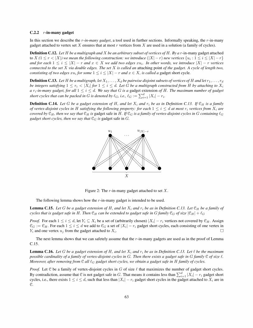
C.2.2 r-in-many gadget
In this section we describe the r-in-many gadget, a tool used in further sections. Informally speaking, the r-in-manygadget attached to vertex set X ensures that at most r vertices from X are used in a solution (a family of cycles).
Definition C.12. LetH be a multigraph andX be an arbitrary subset of vertices ofH . By a r-in-many gadget attachedto X (1 ≤ r < |X|) we mean the following construction: we introduce (|X| − r) new vertices ui : 1 ≤ i ≤ |X| − rand for each 1 ≤ i ≤ |X| − r and x ∈ X we add two edges xui. In other words, we introduce |X| − r verticesconnected to the set X via double edges. The set X is called an attaching point of the gadget. A cycle of length two,constisting of two edges xui for some 1 ≤ i ≤ |X| − r and x ∈ X , is called a gadget short cycle.
Definition C.13. LetH be a multigraph, letX1, . . . , Xd be pairwise disjoint subsets of vertices ofH and let r1, . . . , rdbe integers satisfying 1 ≤ ri < |Xi| for 1 ≤ i ≤ d. Let G be a multigraph constructed from H by attaching to Xi
a ri-in-many gadget, for all 1 ≤ i ≤ d. We say that G is a gadget extension of H . The maximum number of gadgetshort cycles that can be packed in G is denoted by `G, i.e., `G :=
∑di=1 |Xi| − ri.
Definition C.14. Let G be a gadget extension of H , and let Xi and ri be as in Definition C.13. If CH is a familyof vertex-disjoint cycles in H satisfying the following property: for each 1 ≤ i ≤ d at most ri vertices from Xi arecovered by CH , then we say that CH is gadget safe in H . If CG is a family of vertex-disjoint cycles in G containing `Ggadget short cycles, then we say that CG is gadget safe in G.
. . .u1 u|X|−r
X
Figure 2: The r-in-many gadget attached to set X .
The following lemma shows how the r-in-many gadget is intended to be used.
Lemma C.15. Let G be a gadget extension of H , and let Xi and ri be as in Definition C.13. Let CH be a family ofcycles that is gadget safe in H . Then CH can be extended to gadget safe in G family CG of size |CH |+ `G
Proof. For each 1 ≤ i ≤ d, let Yi ⊆ Xi be a set of (arbitrarily chosen) |Xi| − ri vertices not covered by CH . AssignCG := CH . For each 1 ≤ i ≤ d we add to CG a set of |Xi| − ri gadget short cycles, each consisting of one vertex inYi and one vertex uj from the gadget attached to Xi.
The next lemma shows that we can safetely assume that the r-in-many gadgets are used as in the proof of LemmaC.15.
Lemma C.16. Let G be a gadget extension of H , and let Xi and ri be as in Definition C.13. Let ` be the maximumpossible cardinality of a family of vertex-disjoint cycles in G. Then there exists a gadget safe in G family C of size `.Moreover, after removing from C all `G gadget short cycles, we obtain a gadget safe in H family of cycles.
Proof. Let C be a family of vertex-disjoint cycles in G of size ` that maximizes the number of gadget short cycles.By contradiction, assume that C is not gadget safe in G. That means it contains less than
∑di=1 |Xi| − ri gadget short
cycles, i.e., there exists 1 ≤ i ≤ d, such that less than |Xi| − ri gadget short cycles in the gadget attached to Xi are inC.
63
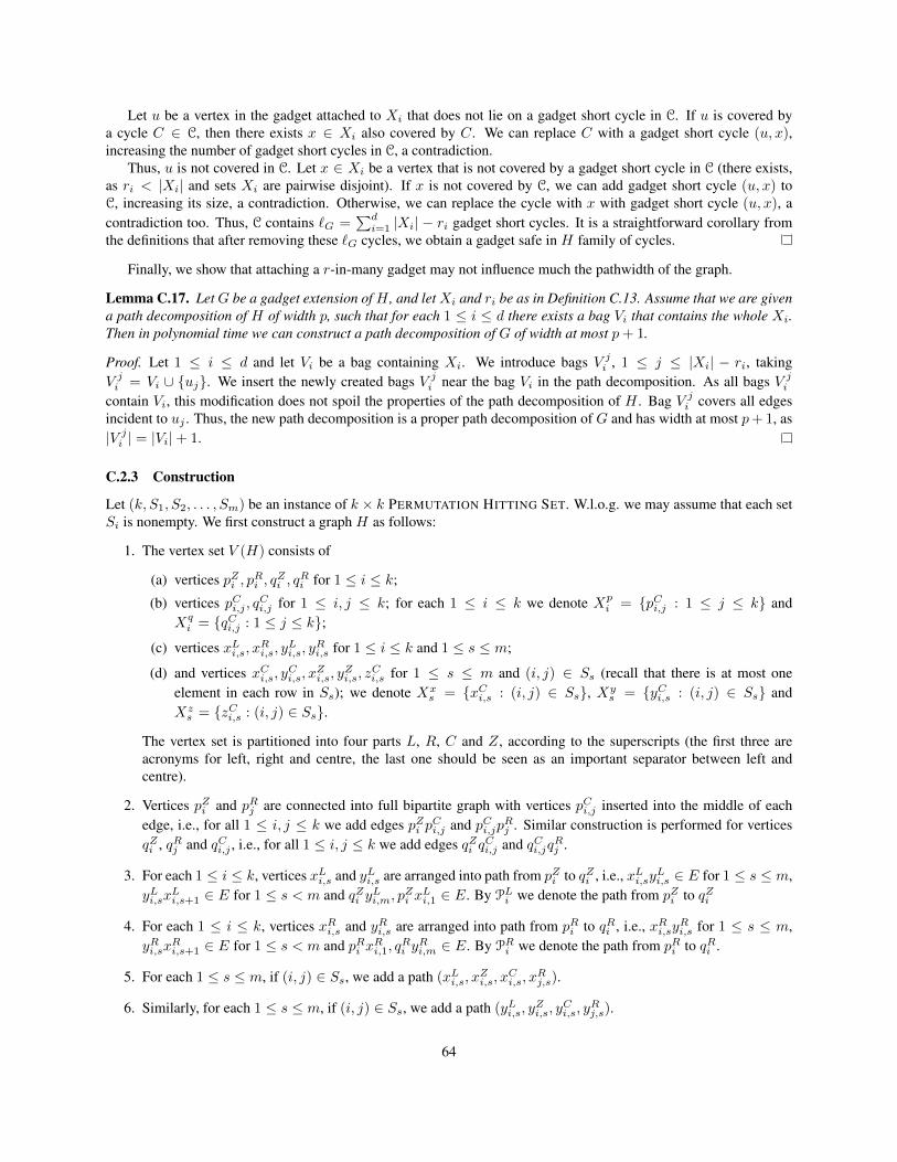
Let u be a vertex in the gadget attached to Xi that does not lie on a gadget short cycle in C. If u is covered bya cycle C ∈ C, then there exists x ∈ Xi also covered by C. We can replace C with a gadget short cycle (u, x),increasing the number of gadget short cycles in C, a contradiction.
Thus, u is not covered in C. Let x ∈ Xi be a vertex that is not covered by a gadget short cycle in C (there exists,as ri < |Xi| and sets Xi are pairwise disjoint). If x is not covered by C, we can add gadget short cycle (u, x) toC, increasing its size, a contradiction. Otherwise, we can replace the cycle with x with gadget short cycle (u, x), acontradiction too. Thus, C contains `G =
∑di=1 |Xi| − ri gadget short cycles. It is a straightforward corollary from
the definitions that after removing these `G cycles, we obtain a gadget safe in H family of cycles.
Finally, we show that attaching a r-in-many gadget may not influence much the pathwidth of the graph.
Lemma C.17. LetG be a gadget extension ofH , and letXi and ri be as in Definition C.13. Assume that we are givena path decomposition of H of width p, such that for each 1 ≤ i ≤ d there exists a bag Vi that contains the whole Xi.Then in polynomial time we can construct a path decomposition of G of width at most p+ 1.
Proof. Let 1 ≤ i ≤ d and let Vi be a bag containing Xi. We introduce bags V ji , 1 ≤ j ≤ |Xi| − ri, takingV ji = Vi ∪ uj. We insert the newly created bags V ji near the bag Vi in the path decomposition. As all bags V jicontain Vi, this modification does not spoil the properties of the path decomposition of H . Bag V ji covers all edgesincident to uj . Thus, the new path decomposition is a proper path decomposition of G and has width at most p+ 1, as|V ji | = |Vi|+ 1.
C.2.3 Construction
Let (k, S1, S2, . . . , Sm) be an instance of k × k PERMUTATION HITTING SET. W.l.o.g. we may assume that each setSi is nonempty. We first construct a graph H as follows:
1. The vertex set V (H) consists of
(a) vertices pZi , pRi , q
Zi , q
Ri for 1 ≤ i ≤ k;
(b) vertices pCi,j , qCi,j for 1 ≤ i, j ≤ k; for each 1 ≤ i ≤ k we denote Xp
i = pCi,j : 1 ≤ j ≤ k andXqi = qCi,j : 1 ≤ j ≤ k;
(c) vertices xLi,s, xRi,s, y
Li,s, y
Ri,s for 1 ≤ i ≤ k and 1 ≤ s ≤ m;
(d) and vertices xCi,s, yCi,s, x
Zi,s, y
Zi,s, z
Ci,s for 1 ≤ s ≤ m and (i, j) ∈ Ss (recall that there is at most one
element in each row in Ss); we denote Xxs = xCi,s : (i, j) ∈ Ss, Xy
s = yCi,s : (i, j) ∈ Ss andXzs = zCi,s : (i, j) ∈ Ss.
The vertex set is partitioned into four parts L, R, C and Z, according to the superscripts (the first three areacronyms for left, right and centre, the last one should be seen as an important separator between left andcentre).
2. Vertices pZi and pRj are connected into full bipartite graph with vertices pCi,j inserted into the middle of eachedge, i.e., for all 1 ≤ i, j ≤ k we add edges pZi p
Ci,j and pCi,jp
Rj . Similar construction is performed for vertices
qZi , qRj and qCi,j , i.e., for all 1 ≤ i, j ≤ k we add edges qZi qCi,j and qCi,jq
Rj .
3. For each 1 ≤ i ≤ k, vertices xLi,s and yLi,s are arranged into path from pZi to qZi , i.e., xLi,syLi,s ∈ E for 1 ≤ s ≤ m,
yLi,sxLi,s+1 ∈ E for 1 ≤ s < m and qZi y
Li,m, p
Zi x
Li,1 ∈ E. By PLi we denote the path from pZi to qZi
4. For each 1 ≤ i ≤ k, vertices xRi,s and yRi,s are arranged into path from pRi to qRi , i.e., xRi,syRi,s for 1 ≤ s ≤ m,
yRi,sxRi,s+1 ∈ E for 1 ≤ s < m and pRi x
Ri,1, q
Ri y
Ri,m ∈ E. By PRi we denote the path from pRi to qRi .
5. For each 1 ≤ s ≤ m, if (i, j) ∈ Ss, we add a path (xLi,s, xZi,s, x
Ci,s, x
Rj,s).
6. Similarly, for each 1 ≤ s ≤ m, if (i, j) ∈ Ss, we add a path (yLi,s, yZi,s, y
Ci,s, y
Rj,s).
64
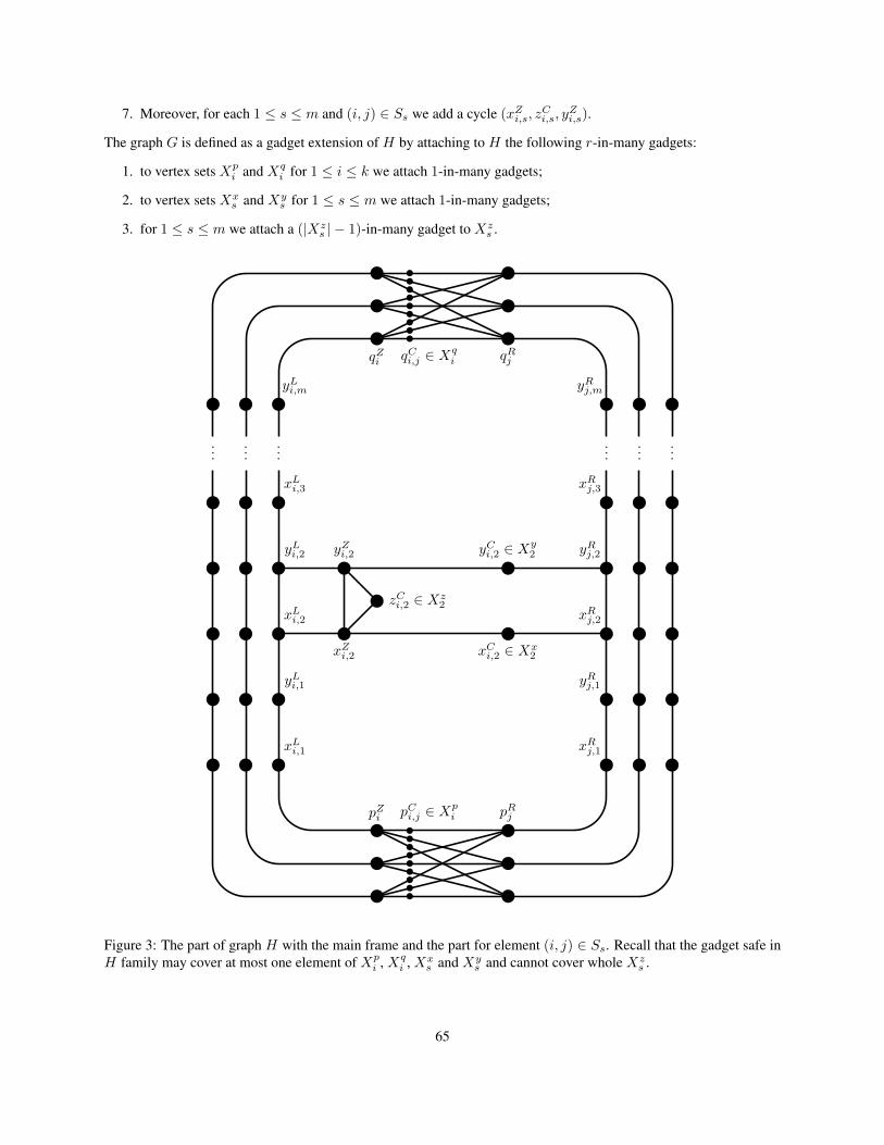
7. Moreover, for each 1 ≤ s ≤ m and (i, j) ∈ Ss we add a cycle (xZi,s, zCi,s, y
Zi,s).
The graph G is defined as a gadget extension of H by attaching to H the following r-in-many gadgets:
1. to vertex sets Xpi and Xq
i for 1 ≤ i ≤ k we attach 1-in-many gadgets;
2. to vertex sets Xxs and Xy
s for 1 ≤ s ≤ m we attach 1-in-many gadgets;
3. for 1 ≤ s ≤ m we attach a (|Xzs | − 1)-in-many gadget to Xz
s .
qZi
......
...
qRj
......
...
qCi,j ∈ Xqi
pZi pRjpCi,j ∈ Xpi
xLi,1
xLi,2
xLi,3
yLi,1
yLi,2
yLi,m
xRj,1
xRj,2
xRj,3
yRj,1
yRj,2
yRj,m
zCi,2 ∈ Xz2
yZi,2
xZi,2
yCi,2 ∈ Xy2
xCi,2 ∈ Xx
2
Figure 3: The part of graph H with the main frame and the part for element (i, j) ∈ Ss. Recall that the gadget safe inH family may cover at most one element of Xp
i , Xqi , Xx
s and Xys and cannot cover whole Xz
s .
65
Clearly, the above construction can be done in polynomial time. Note that we can pack the following number ofgadget short cycles in G:
`G :=
k∑i=1
(|Xpi | − 1 + |Xq
i | − 1) +
m∑s=1
(|Xxs | − 1 + |Xy
s | − 1 + |Xzs | − (|Xz
s | − 1))
= 2k2 − 2k −m+ 2
m∑s=1
|Ss|.
We take ` := k +∑ms=1 |Ss|+ `G, i.e., we ask for ` vertex-disjoint cycles in G.
The following lemma shows the pathwidth bound of G, i.e., proves Point 1.
Lemma C.18. In polynomial time we can construct a path decomposition of G of width 11k.
Proof. By Lemma C.17, it is sufficient to show a path decomposition of H of width 11k − 1 such that each set Xpi ,
Xqi , Xx
s , Xys , Xz
s is contained in some bag.The path decomposition consists of bags V pi for 1 ≤ i ≤ k, Vs for 0 ≤ s ≤ m and V qi for 1 ≤ i ≤ k, arranged in
a path in this order. We define:
1. V pi = pZj , pRj , pCi,j : 1 ≤ j ≤ k for 1 ≤ i ≤ k.
2. V0 = pZi , pRi , xLi,1, xRi,1 : 1 ≤ i ≤ k.
3. Vs = xLi,s, xRi,s, yLi,s, yRi,s, xLi,s+1, xRi,s+1 : 1 ≤ i ≤ k ∪ xCi,s, yCi,s, xZi,s, yZi,s, zCi,s : (i, j) ∈ Ss for 1 ≤ s < m.
4. Vm = xLi,m, xRi,m, yLi,m, yRi,m, qZi , qRi : 1 ≤ i ≤ k ∪ xCi,m, yCi,m, xZi,m, yZi,m, zCi,m : (i, j) ∈ Sm.
5. V qi = qZj , qRj , qCi,j : 1 ≤ j ≤ k for 1 ≤ i ≤ k.
It is easy to see that this is a proper path decomposition of graph H . Moreover, Xpi ⊆ V pi , Xq
i ⊆ V qi andXxs , X
ys , X
zs ⊆ Vs. As for the size bound, note that |V pi | = |V qi | = 3k for 1 ≤ i ≤ k, |V0| = 4k and |Vs| ≤ 11k for
1 ≤ s ≤ m.
Let us note that the above bound is not optimal, but we need only O(k) bound.
C.2.4 From hitting set to cycle cover
We prove Point 2 by the following lemma:
Lemma C.19. If the initial k×k PERMUTATION HITTING SET instance is a YES-instance, then the graphG contains` vertex-disjoint cycles.
Proof. Let S = (i, f(i)) : 1 ≤ i ≤ k be the solution to the k × k PERMUTATION HITTING SET instance. Recallthat S contains exactly one element from each row and exactly one element from each column, thus f is a permutationof [k].
By Lemma C.15, it is sufficient to show a family of cycles C in H that is gadget safe in H and is of size k +∑ms=1 |Ss|.For each 1 ≤ s ≤ m, fix an index 1 ≤ is ≤ k, such that (is, f(is)) ∈ S ∩ Ss. Let
C1 = (xZi,s, yZi,s, zCi,s) : 1 ≤ s ≤ m, 1 ≤ i ≤ k, i 6= is.
Note that C1 is a family of∑ms=1(|Ss| − 1) vertex-disjoint cycles, thus we need to find k +m more.
Fix i, 1 ≤ i ≤ k, and let 1 ≤ s ≤ m : is = i = s1, s2, . . . , sh(i) and s1 < s2 < . . . < sh(i). Consider thefollowing family of h(i) + 1 cycles C(i, j) : 0 ≤ j ≤ h(i):
1. C(i, 0) consists of the path (pZi , pCi,f(i), p
Rf(i)), the subpath of PRf(i) from pRf(i) to xRf(i),s1
, the path (xRf(i),s1, xCi,s1 , x
Zi,s1
, xLi,s1)
and the subpath of PLi from xLi,s1 to pZi ;
66

2. C(i, j) for 1 ≤ j < h(i) consists of the path (yLi,sj , yZi,sj
, yCi,sj , yRf(i),sj
), the subpath of PRf(i) from yRf(i),sjto
xRf(i),sj+1, the path (xRf(i),sj+1
, xCi,sj+1, xZi,sj+1
, xLi,sj+1) and the subpath of PLi from xLi,sj+1
to yLi,sj ;
3. C(i, h(i)) consists of the path (yLi,sh(i) , yZi,sh(i)
, yCi,sh(i) , yRf(i),sh(i)
), the subpath of PRf(i) from yRf(i),sjto qRf(i),
the path (qRf(i), qCi,f(i), q
Zi ) and the subpath of PLi from qZi to yLi,sh(i) .
Note thatC2 = C(i, j) : 1 ≤ i ≤ k, 0 ≤ j ≤ h(i)
is a family of k+m vertex-disjoint cycles in H and they are disjoint with C1. Moreover, C := C1 ∪C2 does not cover:
1. Xpi \ pCi,f(i) and Xq
i \ qCi,f(i) for 1 ≤ i ≤ k;
2. Xxs \ xCis,s and Xy
s \ yCis,s for 1 ≤ s ≤ m;
3. zCis,s ∈ Xzs for 1 ≤ s ≤ m.
Thus C is gadget safe in H . An example showing packing of three cycles for (i, f(i)) ∈ S and h(i) = 2 can be foundin Fig. 4.
C.2.5 From disjoint cycles to hitting set
In this section we prove Point 3 by the following lemma:
Lemma C.20. If the graph G contains at least ` vertex-disjoint cycles, then the initial k×k PERMUTATION HITTINGSET instance is a YES-instance.
Proof. Let CG be a family of vertex-disjoint cycles inGwith maximum possible number of cycles. By the assumption,|CG| ≥ `. By Lemma C.16 we can assume that CG is gadget safe in G and let C ⊆ CG be the gadget safe in H familyof size |CG| − `G ≥ k +
∑ms=1 |Ss|, i.e., C consists of those cycles in CG that are not gadget short cycles.
We now analyze the family C. Informally speaking, we are going to show that C can be placed only in the way asin the proof of Lemma C.19.
First let us analyze subgraph H[L ∪R ∪ C]. Note that this subgraph is a forest containing:
1. k paths PLi for 1 ≤ i ≤ k without the endpoints, i.e., without pZi and qZi ;
2. k trees consisting of paths PRj (1 ≤ j ≤ k) with attached leaves pCi,j , qCi,j for 1 ≤ i ≤ k and xCi,s, y
Ci,s for
1 ≤ s ≤ m, (i, j) ∈ Ss.
3.∑ms=1 |Ss| isolated vertices zCi,s, 1 ≤ s ≤ m, (i, j) ∈ Ss.
Consider now a subgraph ofH induced by L∪R∪C∪a, where a is an arbitrary vertex in Z. Note that this graphis a forest. Indeed, each vertex in Z has at most one edge incident to each connected component of H[L ∪R ∪ C]:
1. for 1 ≤ i ≤ k the vertex pZi is adjacent to xLi,1 on path PLi and vertices pCi,j for 1 ≤ j ≤ k;
2. similarly for 1 ≤ i ≤ k the vertex qZi is adjacent to yLi,m on path PLi and vertices qCi,j for 1 ≤ j ≤ k;
3. for 1 ≤ s ≤ m, (i, j) ∈ Ss the vertex xZi,s is adjacent to zCi,s, xLi,s and xCi,s;
4. similarly for 1 ≤ s ≤ m, (i, j) ∈ Ss the vertex yZi,s is adjacent to zCi,s, yLi,s and yCi,s.
67

qZi
yLi,m
...
qRi
yRf(i),m
...
qCi,f(i) ∈ Xqi
pZi
xLi,1
pRf(i)
xRf(i),1
pCi,f(i) ∈ Xpi
xLi,s1
yLi,s1
xRf(i),s1
yRf(i),s1
......
zCi,s1 ∈ Xzs1
yZi,s1
xZi,s1
yCi,s1 ∈ Xys1
xCi,s1
∈ Xxs1
xLi,s2
yLi,s2
xRf(i),s2
yRf(i),s2
......
zCi,s2 ∈ Xzs2
yZi,s2
xZi,s2
yCi,s2 ∈ Xys2
xCi,s2
∈ Xxs2
Figure 4: An example how to pack three cycles for (i, f(i)) ∈ S and h(i) = 2.
Thus, each cycle from C contains at least two vertices from Z. But, |Z| = 2k+ 2∑ms=1 |Ss| = 2|C|. Thus, each cycle
in C contains exactly two vertices from Z and C covers Z.Let Ci ∈ C be the cycle that covers pZi . The vertex pZi has neighbours xLi,1 and Xp
i . As we are allowed to chooseonly one vertex from Xp
i , the cycle Ci contains a path (xLi,1, pZi , p
Ci,f(i), p
Rf(i)) for some 1 ≤ f(i) ≤ k. If the cycle
Ci contains the edge pRf(i)pCj,f(i) for j 6= i, it contains also pZj and xLj,1. But xLj,1 and xLi,1 are in different connected
components of H[L∪R∪C], thus Ci needs to contain a third vertex in Z, a contradiction. Thus, Ci contains the path(xLi,1, p
Zi , p
Ci,f(i), p
Rf(i), x
Rf(i),1). Note that this in particular implies that f is a permutation of [k].
We claim that S = (i, f(i)) : 1 ≤ i ≤ k is a hitting set in the initial k × k PERMUTATION HITTING SETinstance. It clearly contains exactly one element from each row and from each column. We now show that S ∩Ss 6= ∅for each 1 ≤ s ≤ m.
68

LetZs = pZi : 1 ≤ i ≤ k ∪ xZi,t, yZi,t : 1 ≤ t ≤ s, (i, j) ∈ St ⊆ Z
for 0 ≤ s ≤ m and let
Es = yLi,sxLi,s+1 : 1 ≤ i ≤ k ∪ yRj,sxRj,s+1 : 1 ≤ j ≤ k ⊆ E(H)
for 1 ≤ s < m and letE0 = pZi xLi,1 : 1 ≤ i ≤ k ∪ pRj xRj,1 : 1 ≤ i ≤ k ⊆ E(H).
Note that for 0 ≤ s < m the set Es is a set of 2k edges that separate Zs from Z \ Zs.We now select cycles C(i, s) ∈ C for 1 ≤ i ≤ k and 0 ≤ s ≤ m with the following property: for 1 ≤ i ≤ k and
1 ≤ s < m the edges yLi,sxLi,s+1 and yRf(i),sx
Rf(i),s+1 lie on C(i, s) and for 1 ≤ i ≤ k the edges pLi x
Li,1 and pRf(i)x
Rf(i),1
lie on C(i, 0). Note that cycles C(i, 0) = Ci satisfy the above property. We select cycles C(i, s) by an induction on sand in the s-th step of the induction we prove that there exists 1 ≤ i ≤ k such that (i, f(i)) ∈ Ss.
Let us fix s, 0 ≤ s < m. We show some more properties of cycles C(i, s) : 1 ≤ i ≤ k that we use in theinduction step. Note that each cycle C(i, s) contains two edges from Es and each edge from Es is contained in someC(i, s). Moreover, each edge in Es is in different connected component of H[L ∪ R ∪ C]. Thus, each cycle C(i, s)contains: a subpath of PLi , a subpath of the connected component of H[L ∪ R ∪ C] containing PRf(i), a vertex in Zsand a vertex in Z \ Zs. This in particular implies that cycles C(i, s) : 1 ≤ i ≤ k are pairwise different. As Esseparates Zs from Z \ Zs, each cycle in C \ C(i, s) : 1 ≤ i ≤ k contains either two vertices in Zs, or two verticesin Z \ Zs.
We now perform an induction step. Let 1 ≤ s ≤ m and assume that we have selected cycles C(i, s − 1) for1 ≤ i ≤ k.
Let zCi,s be a (arbitrarily chosen) vertex not covered by C, where (i, j) ∈ Ss. Let us focus on the vertex xZi,s. It hasthree neighbours apart from zCi,s: vertices xLi,s, x
Ci,s and yZi,s. The vertex xCi,s has degree two, and the other neighbour
is xRj,s. As xLi,s ∈ C(i, s − 1) and xRj,s ∈ C(f−1(j), s − 1), the vertex xZi,s lies on C(i, s − 1) or C(f−1(j), s − 1).Both C(i, s− 1) and C(f−1(j), s− 1) are not allowed to cover two vertices from Z \ Zs−1, thus xZi,s and yZi,s lie ondifferent cycles in C. But this means that C(i, s− 1) or C(f−1(j), s− 1) contains the path (xLi,s, x
Zi,s, x
Ci,s, x
Rj,s), thus
C(i, s− 1) = C(f−1(j), s− 1). Since C(i, s− 1) : 1 ≤ i ≤ k are pairwise different, j = f(i) and (i, f(i)) ∈ Ss.Now focus on vertex yZi,s. The vertex xZi,s is used on cycleC(i, s−1), yZi,s /∈ C(i, s−1) and we assumed the vertex
zCi,s is not covered by C. Thus, yZi,s lies on a cycle C with path (yLi,s, yZi,s, y
Ci,s, y
Rf(i),s). As xLi,s, x
Rf(i),s ∈ C(i, s − 1),
and we are allowed to cover only one vertex from Xys , C contains a path (xLi,s+1, y
Li,s, y
Zi,s, y
Ci,s, y
Rf(i),s, y
Rf(i),s+1) (if
s < m) or (qZi , yLi,s, y
Zi,s, y
Ci,s, y
Rf(i),s, q
Rf(i)) (if s = m).
Now focus on vertices xZi′,s for i′ 6= i. As xCi,s is covered by C, the vertex xCi′,s cannot be covered too. Thus, xZi′,sand yZi′,s lie on the same cycle, say Ci
′. As C(i′, s− 1) is not allowed to cover two vertices from Z \Zs−1, the vertex
xLi′,s does not lie on Ci′, thus Ci
′= (xZi′,s, y
Zi′,s, z
Ci′,s).
As vertices xZi′,s and yZi′,s are covered by the cycle (xZi′,s, zCi′,s, y
Zi′,s), the cycle C(i′, s − 1) contains the path
(xLi′,s, yLi′,s, x
Li′,s+1) (if s < m) or (xLi′,s, y
Li′,s, q
Zi′ ) (if s = m). As vertices xCi,s and yCi,s are covered by cyclesC(i, s−1)
and C, the cycle C(i′, s − 1) contains path (xRf(i′),s, yRf(i′),s, x
Rf(i′),s+1) (if s < m) or (xRf(i′),s, y
Rf(i′),s, q
Rf(i′)) (if
s = m).Thus we can put C(i, s) = C and C(i′, s) = C(i′, s − 1) for i′ 6= i and the induction step is performed. As we
maintain the induction step up to s = m, for each 1 ≤ s ≤ m we prove that (i, f(i)) ∈ Ss, thus the initial k × kPERMUTATION HITTING SET instance is a YES-instance.
C.3 From undirected to directed CYCLE PACKING
In this section we provide a reduction from undirected to directed CYCLE PACKING, proving Theorem 5.1 for directedCYCLE PACKING.
69

Lemma C.21. Let (G, `) be an instance of undirected CYCLE PACKING. Then we can construct in polynomial timean equivalent instance (G′, `′) of directed CYCLE PACKING. Moreover, given a path decomposition of G of width p,in polynomial time we can construct a path decomposition of G′ of width at most p+ 3.
Proof. In many problems, a reduction from an undirected version to a directed one is performed by simply changingeach edge uv into pair of arcs (u, v) and (v, u). However, in the case of CYCLE PACKING, such a reduction introducesmany 2-cycles (u, v) that do not have a counterpart in the original undirected graph. We circumvent this problem byadding a directed version of 1-in-many gadget.
To construct graph G′, for each edge e = uv ∈ E(G) we introduce three extra vertices xuve , xvue and ze, and wereplace the edge e with three cycles: (u, xuve , v, xvue ), (xuve , ze) and (xvue , ze). In graphG′ we ask for `′ := `+ |E(G)|vertex-disjoint cycles. The cycles (xuve , ze) and (xvue , ze) are called short cycles.
u
v
u
v
xuve xvu
e
ze
Figure 5: The construction of the gadget replacing edge uv.
First assume that we have a family C of ` vertex-disjoint cycles in G. For each cycle C ∈ C, we orient it in anarbitrary way, and translate it into a cycle C ′ in G′ (i.e., if C goes from u to v via edge e = uv, then in G′ the cycle C ′
uses arcs (u, xuve ) and (xuve , v)). In this way we create a family C′ of ` vertex-disjoint cycles in G′. This family has aproperty that for each e ∈ E(G) at least one vertex xuve and xvue is not covered. Thus we can add a cycle (xuve , ze) or(xvue , ze) to C′, obtaining a family of `′ cycles.
In the other direction, let C′ be a family of vertex-disjoint cycles in G′ that contains maximum possible number ofshort cycles among families of vertex-disjoint cycles of maximum possible size. Assume |C′| ≥ `′.
We claim that C′ contains |E(G)| short cycles. As there are |E(G)| vertices ze, it may not contain more. Assumethat it contains less than |E(G)| short cycles. Let e = uv be an edge, such that ze is not covered by a short cycle. Ifze is not covered by C′, we can add the short cycle (xuve , ze) to C′, possibly deleting a cycle covering xuve . Otherwise,if ze is covered by a cycle C, then xuve or xvue (say xuve ) also belongs to C. But then we can replace C with the cycle(ze, x
uve ). In both cases, we increase the number of short cycles in C′ while not decreasing its size, a contradiction.
Let C be the other ` cycles in C′ that are not short cycles. Each such cycle C ′ does not cover vertices ze, thus ifit covers xuve , it contains a subpath (u, xuve , v). Moreover, either xuve or xvue is covered by a short cycle in C′. ThusC ′ translates into a cycle C in G, by taking an edge e for each vertex xuve visited by C ′. In this way we obtain `vertex-disjoint cycles in G.
We are left with the pathwidth bound. Assume we have a path decomposition of G of width p. We construct a pathdecomposition of G′ in the following way. For each e ∈ E(G), we pick a bag Ve that covers e. We create a new bagV ′e := Ve ∪ xuve , xvue , ze and insert it into the path decomposition near Ve. It is easy to see that this is a proper pathdecomposition of G′ and its width is at most p+ 3.
70
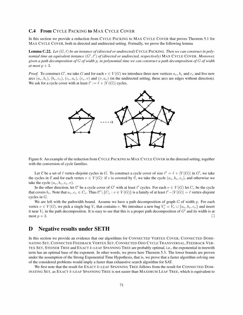
C.4 From CYCLE PACKING to MAX CYCLE COVER
In this section we provide a reduction from CYCLE PACKING to MAX CYCLE COVER that proves Theorem 5.1 forMAX CYCLE COVER, both in directed and undirected setting. Formally, we prove the following lemma
Lemma C.22. Let (G, `) be an instance of (directed or undirected) CYCLE PACKING. Then we can construct in poly-nomial time an equivalent instance (G′, `′) of (directed or undirected, respectively) MAX CYCLE COVER. Moreover,given a path decomposition of G of width p, in polynomial time we can construct a path decomposition of G of widthat most p+ 3.
Proof. To construct G′, we take G and for each v ∈ V (G) we introduce three new vertices av , bv and cv and five newarcs (av, bv), (bv, cv), (cv, av), (cv, v) and (v, av) (in the undirected setting, these arcs are edges without direction).We ask for a cycle cover with at least `′ := `+ |V (G)| cycles.
Figure 6: An example of the reduction from CYCLE PACKING to MAX CYCLE COVER in the directed setting, togetherwith the conversion of cycle families.
Let C be a set of ` vertex-disjoint cycles in G. To construct a cycle cover of size `′ = ` + |V (G)| in G′, we takethe cycles in C and for each vertex v ∈ V (G): if v is covered by C, we take the cycle (av, bv, cv), and otherwise wetake the cycle (av, bv, cv, v).
In the other direction, let C′ be a cycle cover of G′ with at least `′ cycles. For each v ∈ V (G) let Cv be the cyclethat covers bv . Note that av, cv ∈ Cv . Thus C′\Cv : v ∈ V (G) is a family of at least `′−|V (G)| = ` vertex-disjointcycles in G.
We are left with the pathwidth bound. Assume we have a path decomposition of graph G of width p. For eachvertex v ∈ V (G), we pick a single bag Vv that contains v. We introduce a new bag V ′v = Vv ∪ av, bv, cv and insertit near Vv in the path decomposition. It is easy to see that this is a proper path decomposition of G′ and its width is atmost p+ 3.
D Negative results under SETHIn this section we provide an evidence that our algorithms for CONNECTED VERTEX COVER, CONNECTED DOMI-NATING SET, CONNECTED FEEDBACK VERTEX SET, CONNECTED ODD CYCLE TRANSVERSAL, FEEDBACK VER-TEX SET, STEINER TREE and EXACT k-LEAF SPANNING TREE are probably optimal, i.e., the exponential in treewithterm has an optimal base of the exponent. In other words, we prove here Theorem 5.3. The lower bounds are provenunder the assumption of the Strong Exponential Time Hypothesis, that is, we prove that a faster algorithm solving oneof the considered problems would imply a faster than exhaustive search algorithm for SAT.
We first note that the result for EXACT k-LEAF SPANNING TREE follows from the result for CONNECTED DOM-INATING SET, as EXACT k-LEAF SPANNING TREE is not easier than MAXIMUM LEAF TREE, which is equivalent to
71

CONNECTED DOMINATING SET [25]. Second, note that the lower bound for STEINER TREE follows from the lowerbound for CONNECTED VERTEX COVER by the following simple reduction.
Lemma D.1. Given a CONNECTED VERTEX COVER instance (G, k) together with a tree decomposition ofG of widtht (or path decomposition of G of width p), one can construct in polynomial time an equivalent instance (G′, T, k′)of STEINER TREE together with a tree decomposition of G′ of width t (or path decomposition of G of width at mostp+ 1, respectively).
Proof. Given the instance (G, k), we construct the instance (G′, T, k′) by subdiving each edge ofGwith a terminal andsetting k′ = |T |+ k (i.e., we replace each edge e = uv in G with a path u,we, v and we take T = we : e ∈ E(G)).It is easy to see that G contains a connected vertex cover of size at most k if and only if (G′, T ) contains a Steiner treeof cardinality at most k + |T | = k + |E(G)|.
Moreover, given a tree decomposition T of G of width t, we can construct a tree decomposition T′ of G′ of widthat most t in the following manner. If G is a forest, G′ is a forest too and we construct the optimal tree decompositionof G′ in polynomial time. Otherwise, t ≥ 2 and for each e ∈ E(G) we pick one fixed node x(e) whose bag coverse. We first set T′ := T and then, for each uv = e ∈ E(G), we attach a leaf node y(e) to the node x(e) with the bagBy(e) = u, v, we.
In the case of a path decomposition T of G of width p, we can construct a path decomposition T′ of G′ of width atmost p+ 1 in the following manner. For each e ∈ E(G) we pick one fixed node x(e) whose bag covers e. We first setT′ := T and then, sequentially for each uv = e ∈ E(G), we create a new node y(e) with the bagBy(e) = Bx(e)∪weand insert it immediately after the node x(e) on the path decomposition.
Thus we are left with the first five problems of Theorem 5.3. In the proofs we follow the same approach asLokshtanov et al [47] in the lower bounds for problems without the connectivity requirement. We mostly base on theVERTEX COVER and DOMINATING SET lower bounds of [47], however our gadgets are adjusted to the consideredproblems. For each problem we show a polynomial-time construction that, given a SAT instance with n variables,constructs an equivalent instance of the considered problem, together with a path decomposition of the underlyinggraph of width roughly log3(2n) = n/ log 3 in the case of CONNECTED VERTEX COVER and FEEDBACK VERTEXSET and of width roughly log4(2n) = n/2 in the case of the other problems. Thus, each of the following subsectionsconsists of three parts. First, we give a construction procedure that, given a SAT formula Φ, produces an instance ofthe considered problem. Second, we prove that the constructed instance is equivalent to the formula Φ. Finally, weshow the claimed pathwidth bound.
Similarly as in [47], we prove pathwidth bounds for the constructed graphs using mixed search game. Let us recallthe definition from [47].
Definition D.2 ([59, 47]). In a mixed search game, a graph G is considered as a system of tunnels. Initially, all edgesare contaminated by a gas. An edge is cleared by placing searchers at both its end-points simultaneously or by slidinga searcher along the edge. A cleared edge is re-contaminated if there is a path from an uncleared edge to the clearededge without any searchers on its vertices or edges. A search is a sequence of operations that can be of the followingtypes: (a) placement of a new searcher on a vertex; (b) removal of a searcher from a vertex; (c) sliding a searcheron a vertex along an incident edge and placing the searcher on the other end. A search strategy is winning if after itstermination all edges are cleared. The mixed search number of a graph G, denoted ms(G), is the minimum number ofsearchers required for a winning strategy of mixed searching on G.
Proposition D.3 ([59]). For a graph G, pw(G) ≤ ms(G) ≤ pw(G) + 1.
Moreover, in each case considered by us, the presented cleaning strategy easily yield a polynomial time algorithmthat constructs a path decomposition of G of width not greater than the number of searchers used.
D.1 CONNECTED VERTEX COVER
Theorem D.4. Assuming SETH, there cannot exist a constant ε > 0 and an algorithm that given an instance (G =(V,E), k) together with a path decomposition of the graph G of width p solves the CONNECTED VERTEX COVERproblem in (3− ε)p|V |O(1) time.
72
Construction Given ε > 0 and an instance Φ of SAT with n variables and m clauses we construct a graph G asfollows. We first choose a constant integer η, which value depends on ε only. The exact formula for η is presentedlater. We partition variables of Φ into groups F1, . . . , Fn′ , each of size at most β = blog 3ηc, hence n′ = dn/βe. Notethat now ηn′ ∼ n/ log 3, the pathwidth of G will be roughly ηn′.
First, we add to the graph G two vertices r and r∗, connected by an edge. In the graph G the vertex r∗ will be ofdegree one, thus any connected vertex cover of G needs to include r. The vertex r is called a root.
Second, we take a = m(2ηn′ + 1) and for each 1 ≤ t ≤ n′ and 1 ≤ ` ≤ η we create a path Pt,` consisting of 2avertices vαt,`,k, 0 ≤ k < a and 1 ≤ α ≤ 2, arranged in the following order:
v1t,`,0, v
2t,`,0, v
1t,`,1, . . . , v
1t,`,a−1, v
2t,`,a−1.
Furthermore we connect all vertices v2t,`,k (0 ≤ k < a) and v1
t,`,0 to the root r. To simplify further notation we denotev1t,`,a = r. Let V be the set of all vertices on all paths Pt,`.
We now provide a description of a group gadget Bt,k, which will enable us to encode 2β possible assignmentsof one group of β variables. Fix a block Ft, 1 ≤ t ≤ n′, and a position k, 0 ≤ k < a. For each 1 ≤ ` ≤ η wecreate three vertices hαt,`,k, 1 ≤ α ≤ 3 that are pairwise adjacent and all are adjacent to the root r. Moreover, weadd edges h1
t,`,kv1t,`,k, h2
t,`,kv2t,`,k and h3
t,`,kv1t,`,k+1. Let Ht,`,k = hαt,`,k : 1 ≤ α ≤ 3, Ht,k =
⋃η`=1 Ht,`,k. and
H =⋃n′t=1
⋃a−1k=0 Ht,k. Note that each (connected) vertex cover in G needs to include at least two out of three vertices
from each set Ht,`,k.In order to encode 2β assignments we consider subsets of Ht,k that contain exactly one vertex out of each set
Ht,`,k. For a sequence S = (s1, . . . , sη) ∈ 1, 2, 3η by S(Ht,k) we denote the set hs`t,`,k : 1 ≤ ` ≤ η. For eachsequence S ∈ 1, 2, 3η we add three vertices xSt,k, xS∗t,k and ySt,k, where xSt,k is also adjacent to all the vertices ofS(Ht,k) (recall that η and β are constants depending only on ε). We add edges xSt,kx
S∗t,k, xSt,ky
St,k and ySt,kr. In the
graph G the vertices xS∗t,k are of degree one, thus any connected vertex cover in G needs to include all vertices xSt,k.
Let Yt,k = ySt,k : S ∈ 1, 2, 3η for 1 ≤ t ≤ n′, 0 ≤ k < a and Y =⋃n′t=1
⋃a−1k=0 Yt,k.
Additionally we add two adjacent vertices zt,k and z∗t,k and connect zt,k to vertices ySt,k for all S ∈ 1, 2, 3η .Again, the vertex z∗t,k is of degree one in G and forces zt,k to be included in any connected vertex cover of G.
The above step finishes the construction of the group gadgets needed to encode an assignment and now we addvertices used to check the satisfiability of the formula Φ. Observe that for a group of variables Ft there are at most 2β
possible assignments and there are 3η ≥ 2β vertices xSt,k for sequences S from the set 1, 2, 3η in each group gadgetBt,k, hence we can assign a unique sequence S to each assignment. Let C0, . . . , Cm−1 be the clauses of the formulaΦ. For each clause Ci we create (2ηn′ + 1) pairs of adjacent vertices ci,j and c∗i,j , one for each 0 ≤ j < (2ηn′ + 1).The vertex c∗i,j is of degree one in G and therefore forces any connected vertex cover of G to include ci,j . The vertexci,j can only be connected to gadgets Bt,mj+i for 1 ≤ t ≤ n′. For each group of variables Ft we consider allsequences S ∈ 1, 2, 3η that correspond to an assignment of Ft satisfying the clause Ci (i.e., one of the variables ofFt is assigned a value such that Ci is already satisfied). For each such sequence S and for each 0 ≤ j < (2ηn′ + 1)we add an edge ySt,mj+ici,j .
We can view the whole construction as a matrix of group gadgets, where each row corresponds to some group ofvariables Ft and each column is devoted to some clause in such a way that each clause gets (2ηn′+1) private columns(but not consecutive) of the group gadget matrix, as in Figure 8.
Finally, let K = ηn′ · 3a+ (3η + 2)n′a+ a+ 1 be the size of the vertex cover we ask for.
Correctness
Lemma D.5. If Φ has a satisfying assignment, then there exists a connected vertex cover in G of size K.
Proof. Given a satisfying assignment φ of the formula Φ we construct a connected vertex cover X ⊆ V as follows.Let Xforce be the set of vertices that are forced to be in any connected vertex cover of G, that is r, ci,j for 0 ≤ i < m,0 ≤ j < (2ηn′ + 1), xSt,k for 1 ≤ t ≤ n′, 0 ≤ k < m(2ηn′ + 1), S ∈ 1, 2, 3η and zt,k for 1 ≤ t ≤ n′,0 ≤ k < m(2ηn′ + 1). Note that |Xforce| = 1 + a+ (3η + 1)n′a.
73

zt,k
x(3,3,2)t,k
y(3,3,2)t,k
v1t,1,k v2t,1,k v1t,1,k+1
h1t,1,k
h2t,1,k
h3t,1,k
v1t,2,k v2t,2,k v1t,2,k+1
h1t,2,k
h2t,2,k
h3t,2,k
v1t,3,k v2t,3,k v1t,3,k+1
h1t,3,k
h2t,3,k
h3t,3,k
Figure 7: Group gadget Bt,k for η = 3. Dashed edges are connecting a vertex with the root r. Vertices that have apendant neighbour and thus need to be included in any connected vertex cover of G are presented as squares.
For each group of variables Ft we consider the sequence St ∈ 1, 2, 3η which corresponds to the restriction ofthe assignment φ to the variables of Ft. Let
Xh =
n′⋃t=1
a−1⋃k=0
η⋃`=1
hαt,`,k : α 6= St(`).
The set Xh includes exactly two vertices out of each set Ht,`,k, thus |Xh| = ηn′ · 2a. Moreover, we define the set Xv
to contain all vertices v2t,`,k if St(`) = 2, and all vertices v1
t,`,k otherwise (1 ≤ t ≤ n′, 1 ≤ ` ≤ η, 0 ≤ k < a). The setXv includes every other vertex on each path Pt,`, thus |Xv| = ηn′a.
Finally, let us define the set Xy to be the set of all vertices yStt,k for all 1 ≤ t ≤ n′ and 0 ≤ k < a. LetX = Xforce ∪Xh ∪Xv ∪Xy . Note that as |Xy| = n′a we have |X| = K. We now verify that X is a connected vertexcover of G.
First, we verify that G \X is an edgeless graph.
1. The vertices r∗, c∗i,j , xS∗t,k and z∗t,k are isolated in G \X , as their single neighbours in G are included in Xforce.
2. The vertices vαt,`,k that are not in X are isolated in G \X , as Xv contains every other vertex on each path Pt,`and we chose α in such a manner that the neighbours of vαt,`,k from H are in Xh.
3. The vertices hSt(`)t,`,k are isolated in G \ X , since their single neighours on paths Pt,` are in Xv and all other
neighbours of hSt(`)t,`,k are in Xforce and in Xh.
4. Finally, the vertices ySt,k are isolated in G \X since their neighbourhoods are contained in Xforce.
To finish the proof we need to verify that G[X] is connected. We ensure it by showing that in G[X] each vertex inX is connected to the root r.
1. The claim is obvious for Xh and Xy , as they are contained in the neighbourhood of r.
74

r
Bn′,0 Bn′,a−1
B1,0 B1,a−1
ci,j
Figure 8: Gray rectangles represent group gadgets. Dashed edges connect have the root vertex r as one of the end-points. Vertices that have a pendant neighbour and thus need to be included in any connected vertex cover of G arepresented as squares.
2. If vertices v2t,`,k belong to Xv , they are connected to r by direct edges. Otherwise, the vertices v1
t,`,k areconnected via vertices h1
t,`,k or h3t,`,k−1 (with the exception of vertices v1
t,`,0 that are connected directly).
3. Each vertex xSt,k for S 6= St is connected to r via any vertex hS(`)t,`,k for which S(`) 6= St(`).
4. Vertices xStt,k and zt,k are connected to r via yStt,k.
75
5. Finally, each vertex ci,k is connected to r via any vertex yStt,k for which the assignment φ on variables from Ftsatisfies the clause Ci.
Lemma D.6. If there exists a connected vertex cover X of size at most K in the graph G, then Φ has a satisfyingassignment.
Proof. As in the previous lemma, let Xforce be the set of vertices that are forced to be in any connected vertex cover ofG, that is r, ci,j for 1 ≤ i ≤ m, 0 ≤ j < (2ηn′ + 1), xSt,k for 1 ≤ t ≤ n′, 0 ≤ k < m(2ηn′ + 1), S ∈ 1, 2, 3η andzt,k for 1 ≤ t ≤ n′, 0 ≤ k < m(2ηn′ + 1). Note that |Xforce| = 1 + a+ (3η + 1)n′a and Xforce ⊆ X .
Let Xv = X ∩ V, Xh = X ∩H and Xy = X ∩ Y. Note that
1. Xv needs to include at least a vertices from each path Pt,`, thus |Xv| ≥ ηn′a.
2. Xh needs to include at least two vertices out of each set Ht,`,k, thus |Xh| ≥ ηn′ · 2a.
3. Xy needs to include at least one vertex ySt,k for each 1 ≤ t ≤ n′ and 0 ≤ k < a to ensure that the vertex zt,k isconnected to the root r in G[X]. Thus |Xy| ≥ n′a.
As |X| ≤ K, we have |Xv| = ηn′a, |Xh| = ηn′ · 2a, |Xy| = n′a and |X| = K.As |Xh| = ηn′ · 2a, for each 1 ≤ t ≤ n′, 1 ≤ ` ≤ η and 0 ≤ k < a we have |Xh ∩Ht,`,k| = 2. This allows us to
define a sequence St,k ∈ 1, 2, 3η satisfying hSt,k(`)t,`,k /∈ Xh for 1 ≤ ` ≤ η.
Note that the vertex xSt,kt,k ∈ Xforce does not have a neighbour in Xh, thus, to connect it to the root r, we need to
have ySt,kt,k ∈ Xy . As |Xy| = n′a, we infer that |Yt,k ∩X| = 1 for all 1 ≤ t ≤ n′ and 0 ≤ k < a, i.e., ySt,k ∈ X if andonly if S = St,k.
We now show that for fixed t the sequences St,k cannot differ much for 0 ≤ k < a. As |Xv| = ηn′a, for each1 ≤ t ≤ n′, 1 ≤ ` ≤ η and 0 ≤ k ≤ a we have that |Xv ∩ vαt,`,k : 1 ≤ α ≤ 2| = 1. Let α(t, `, k) be such that
vα(t,`,k)t,`,k ∈ Xv . Now note that for 1 ≤ t ≤ n′, 1 ≤ ` ≤ η and 0 ≤ k < a− 1:
1. If St,k(`) = 3, then α(t, `, k + 1) = 1, as otherwise the edge v1t,`,k+1h
3t,`,k is not covered by X . More-
over, h1t,`,k+1 ∈ Xh, as otherwise v1
t,`,k+1 is isolated in G[X], and h2t,`,k+1 ∈ Xh, as otherwise the edge
v2t,`,k+1h
2t,`,k+1 is not covered by X . Thus St,k+1(`) = 3 as well.
2. If St,k(`) = 1 then α(t, `, k) = 1, as otherwise the edge v1t,`,kh
1t,`,k is not covered by X . Thus α(t, `, k +
1) = 1, as otherwise the edge v2t,`,kv
1t,`,k+1 is not covered by X , and St,k+1(`) 6= 2, as otherwise the edge
v2t,`,k+1h
2t,`,k+1 is not covered by X .
For fixed 1 ≤ t ≤ n′ and 1 ≤ ` ≤ η define the sequence St,`(k) = St,k(`). From the above arguments we inferthat the sequence St,`(k) cannot change more than twice. As a = m(2ηn′+ 1), we conclude that there exists an index0 ≤ j < (2ηn′ + 1) such that for all 1 ≤ t ≤ n′, 1 ≤ ` ≤ η the sequence St,`(mj + i) is constant for 0 ≤ i < m.
We create now an assignment φ by taking, for each group of variables Ft, an assignment corresponding to thesequence St,mj . Now we prove that φ satisfies Φ. Take any clauseCi, 0 ≤ i < m, and focus on the vertex ci,j ∈ Xforce.The vertex ci,j needs to be connected to the root r in G[X], thus for some 1 ≤ t ≤ n′ and S ∈ 1, 2, 3η we haveySt,mj+i ∈ X and the assignment of Ft that corresponds to S satisfies Ci. However, we know that ySt,mj+i ∈ X impliesthat S = St,mj+i, and thus φ satisfies Ci.
Pathwidth bound
Lemma D.7. Pathwidth of the graph G is at most ηn′ +O(3η). Moreover a path decomposition of such width can befound in polynomial time.
76
Proof. We give a mixed search strategy to clean the graph with ηn′ +O(3η) searchers. First we put a searcher in thevertex r∗ and slide it to the root r. This searcher remains there till the end of the cleaning process.
For a gadget Bt,k we call the vertices v1t,`,k and v1
t,`,k+1, 1 ≤ ` ≤ η, as entry vertices and exit vertices respectively.We search the graph in a = m(2ηn′ + 1) rounds. At the beginning of round k (0 ≤ k < a) there are searchers on theentry vertices of the gadget Bt,k for every 1 ≤ t ≤ n′. Let 0 ≤ i < m and 0 ≤ j < (2ηn′ + 1) be integers such thatk = i+mj. We place a searcher on c∗i,j and slide it to ci,j . Then, for each 1 ≤ t ≤ n′ in turn we:
• put O(3η) searchers on all vertices of the group gadget Bt,k,
• put 2η searchers on all vertices v2t,`,k and v1
t,`,k+1, 1 ≤ ` ≤ η,
• remove searchers from all vertices of the group gadget Bt,k and vαt,`,k for 1 ≤ ` ≤ η and 1 ≤ α ≤ 2.
The last step of the round is removing a searcher from the vertex ci,j . After the last round the whole graph G iscleaned. Since we reuse O(3η) searchers for cleaning group gadgets, ηn′+O(3η) searchers suffice to clean the graph.
Using the above graph cleaning process a path decomposition of width ηn′+O(3η) can be constructed in polyno-mial time.
Proof of Theorem D.4. Suppose CONNECTED VERTEX COVER can be solved in (3 − ε)p|V |O(1) time provided thatwe are given a path decomposition of G of width p. Let λ = log3(3 − ε) < 1. We choose η large enough such that
log 3η
blog 3ηc <1λ . Given an instance of SAT we construct an instance of CONNECTED VERTEX COVER using the above
construction and the chosen value of η. Next we solve CONNECTED VERTEX COVER using the 3λp|V |O(1) timealgorithm. Lemmata D.5, D.6 ensure correctness, whereas Lemma D.7 implies that running time of our algorithm is3ληn
′ |V |O(1), however we have
3ληn′
= 2ληn′ log 3 = 2λn
′ log 3η ≤ 2C · 2λn log 3η/blog 3ηc = 2C · 2λ′n
for some λ′ < 1 and C = λ log 3η . This concludes the proof.
D.2 CONNECTED DOMINATING SET
Theorem D.8. Assuming SETH, there cannot exist a constant ε > 0 and an algorithm that given an instance (G =(V,E), k) together with a path decomposition of the graph G of width p solves the CONNECTED DOMINATING SETproblem in (4− ε)p|V |O(1) time.
Construction Given ε > 0 and an instance Φ of SAT with n variables and m clauses we construct a graph G asfollows. We assume that the number of variables n is even, otherwise we add a single dummy variable. We partitionvariables of Φ into groups F1, . . . , Fn′ , each of size two, hence n′ = n/2. The pathwidth of G will be roughly n′.
First, we add to the graph G two vertices r and r∗, connected by an edge. In the graph G the vertex r∗ is of degreeone, thus any connected dominating set of G needs to include r. The vertex r is called a root.
Second, we take a = m(n+ 1) and for each 1 ≤ t ≤ n′ we create a path Pt consisting of 4a vertices vαt,k and hαt,k,0 ≤ k < a and 1 ≤ α ≤ 2. On the path Pt the vertices are arranged in the following order:
v1t,0, h
1t,0, v
2t,0, h
2t,0, v
1t,1, . . . , h
2t,a−1.
Let V and H be the sets of all vertices vαt,k and hαt,k (1 ≤ t ≤ n′, 0 ≤ k < a, 1 ≤ α ≤ 2), respectively. Weconnect vertices v1
t,0 and all vertices in H to the root r. To simplify further notation we denote v1t,a = r, note that
h2t,a−1v
1t,a ∈ E.
Third, for each 1 ≤ t ≤ n′ and 0 ≤ k < a we introduce guard vertices p1t,k, p2
t,k and qt,k. Each guard vertex is ofdegree two in G, namely p1
t,k is adjacent to v1t,k and v2
t,k, p2t,k is adjacent to v2
t,k and v1t,k+1 and qt,k is adjacent to h1
t,k
and h2t,k. Thus, each guard vertex ensures that at least one of its neighbours is contained in any connected dominating
set in G.
77

v11,0 v21,0
h11,0 h2
1,0q1,0
p11,0 p21,0
v12,0 v22,0
h12,0 h2
2,0q2,0
p12,0 p22,0
v11,1 v21,1
h11,1 h2
1,1q1,1
p11,1 p21,1
v12,1 v22,1
h12,1 h2
2,1q2,1
p12,1 p22,1
v11,2 v21,2
h11,2 h2
1,2q1,2
p11,2 p21,2
v12,2 v22,2
h12,2 h2
2,2q2,2
p12,2 p22,2
v11,4
v12,4
c1,0
Figure 9: Part of the construction for CONNECTED DOMINATING SET. Dashed edges are connecting a vertex withthe root r. Empty circles represent guard vertices.
The intuition of the construction made so far is as follows. For each two-variable block Ft we encode any assign-ment of the variables in Ft as a choice whether to take v1
t,k or v2t,k and h1
t,k or h2t,k to the connected dominating set in
G.We have finished the part of the construction needed to encode an assignment and now we add vertices used to
check the satisfiability of the formula Φ. Let C0, . . . , Cm−1 be the clauses of the formula Φ. For each clause Ci wecreate (n+ 1) vertices ci,j , one for each 0 ≤ j < n+ 1. Consider a clause Ci and a group of variables Ft = x1
t , x2t.
If x1t occurs positively in Ci then we connect ci,j with v1
t,mj+i and if x1t occurs negatively in Ci then we connect ci,j
with v2t,mj+i. Similarly if x2
t occurs positively inCi then we connect ci,j with h1t,mj+i and if x2
t occurs negatively inCithen we connect ci,j with h2
t,mj+i. Intuitively taking the vertex v1t,mj+i into a connected dominating set corresponds
to setting x1t to true, whereas taking the vertex h1
t,mj+i into a connected dominating set corresponds to setting x2t to
true.We can view the whole construction as a matrix, where each row corresponds to some group of variables Ft and
each column is devoted to some clause in such a way that each clause gets (n+1) private columns (but not consecutive)of the matrix.
Finally, let K = 1 + n′ · 2a be the size of the connected dominating set we ask for.
Correctness
Lemma D.9. If Φ has a satisfying assignment, then there exists a connected dominating set X in the graph G of sizeK.
Proof. Given a satisfying assignment φ of the formula Φ we construct a connected dominating set X as follows. Foreach block Ft = x1
t , x2t and for each 0 ≤ k < a we include into X:
1. the vertex v1t,k if φ(x1
t ) is true, and v2t,k otherwise;
2. the vertex h1t,k if φ(x2
t ) is true, and h2t,k otherwise.
Finally, we put r into X . Note that |X| = 1 + n′ · 2a = K. We now verify that X is a connected dominating set in G.First, we verify that X dominates all vertices in G.
1. r∗ and all vertices in H are dominated by the root r.
78

2. All guards p1t,k, p2
t,k and q1t,k are dominated by X ∩ (H ∪ V) (with the possible exception of p2
t,a−1 that isdominated by r).
3. All vertices in V are dominated by X ∩H (with the possible exception of v1t,0 that is dominated by r).
4. Finally, each clause vertex ci,j is dominated by any vertex vαt,mj+i or hαt,mj+i that corresponds to a variable thatsatisfies Ci in the assignment φ.
To finish the proof we need to ensure that G[X] is connected. We prove this by showing that each vertex in X isconnected to the root r inG[X]. This is obvious for vertices inX∩H, as H ⊆ NG(r). Moreover, for each 1 ≤ t ≤ n′and 0 ≤ k < a:
1. if v1t,k ∈ X , then v1
t,k is connected to the root via h2t,k−1 or h1
t,k, with the exception of v1t,0, that is connected to
r directly;
2. if v2t,k ∈ X , then v2
t,k is connected to the root via h1t,k or h2
t,k.
Lemma D.10. If there exists a connected dominating set X of size at most K in the graph G, then Φ has a satisfyingassignment.
Proof. First note that the vertex r∗ ensures that r ∈ X . Moreover, the guard vertices p1t,k and qt,k ensure that for
each 1 ≤ t ≤ n′ and 0 ≤ k < a at least one vertex vαt,k and at least one vertex hαt,k (1 ≤ α ≤ 2) belongs to X . As|X| ≤ 1 + n′ · 2a and we have n′ · 2a aforementioned guards with disjoint neighbourhoods, for each 1 ≤ t ≤ n′ and0 ≤ k < a exactly one vertex vαt,k and exactly one vertex hαt,k belongs to X . Moreover, X ⊆ r ∪ V ∪H.
For each 0 ≤ k < a we construct an assignment φk as follows. For each block Ft = x1t , x
2t we define:
1. φk(x1t ) to be true if v1
t,k ∈ X and false if v2t,k ∈ X;
2. φk(x2t ) to be true if h1
t,k ∈ X and false if h2t,k ∈ X .
We now show that the assignments φk cannot differ much for all indices 0 ≤ k < a. Note that for each blockFt = x1
t , x2t and 0 ≤ k < a− 1:
1. if φk(x1t ) is true, then φk+1(x1
t ) is also true, as otherwise v2t,k, v
1t,k+1 /∈ X and the guard p2
t,k is not dominatedby X;
2. if φk(x2t ) is true, then φk+1(x2
t ) is also true, as otherwise h2t,k, h
1t,k+1 /∈ X and the vertex v2
t,k is either notdominated by X (if v2
t,k /∈ X) or isolated in G[X] (if v2t,k ∈ X).
For each variable x we define a sequence φx(k) = φk(x), 0 ≤ k < a. From the reasoning above we infer that foreach variable x the sequence φx(k) can change its value at most once, from false to true. Thus, as a = m(n+ 1), weconclude that there exists 0 ≤ j < n+ 1 such that for all 0 ≤ i < m the assignments φmj+i are equal.
We claim that the assigment φ = φmj satisfies Φ. Consider a clause Ci and focus on the vertex ci,j . It is notcontained in X , thus one of its neighbour is contained in X . As this neighbour corresponds to an assignment of onevariable that both satisfies Ci (by the construction process) and is consistent with φmj+i = φ (by the definition ofφmj+i), the assignment φ satisfies Ci and the proof is finished.
Pathwidth bound
Lemma D.11. Pathwidth of the graph G is at most n′ + O(1). Moreover a path decomposition of such width canfound in polynomial time.
79

Proof. We give a mixed search strategy to clean the graph with n′ + 9 searchers. First we put a searcher in the vertexr∗ and slide it to the root r. This searcher remains there till the end of the cleaning process.
We search the graph in a = m(n+ 1) rounds. At the beginning of round k (0 ≤ k < a) there are searchers on allvertices v1
t,k for 1 ≤ t ≤ n′. Let 0 ≤ i < m and 0 ≤ j < n+ 1 be integers such that k = i+mj. We place a searcheron ci,j . Then, for each 1 ≤ t ≤ n′ in turn we put 7 searchers on vertices p1
t,k, v2t,k, p2
t,k, v1t,k+1, h1
t,k, h2t,k and qt,k, and
then remove 7 searchers from vertices v1t,k, p1
t,k, v2t,k, p2
t,k, h1t,k, h2
t,k and qt,k. The last step of the round is removinga searcher from the vertex ci,j . After the last round the whole graph G is cleaned. Since we reuse 8 searchers in thecleaning process, n′ + 9 searchers suffice to clean the graph.
Using the above graph cleaning process a path decomposition of width n′+O(1) can be constructed in polynomialtime.
Proof of Theorem D.8. Suppose CONNECTED DOMINATING SET can be solved in (4−ε)p|V |O(1) time provided thatwe are given a path decomposition ofG of width p. Given an instance of SAT we construct an instance of CONNECTEDDOMINATING SET using the above construction and solve it using the (4− ε)p|V |O(1) time algorithm. Lemmata D.9,D.10 ensure correctness, whereas Lemma D.11 implies that running time of our algorithm is (4 − ε)n/2|V |O(1),however we have (4− ε)n/2 = (
√4− ε)n and
√4− ε < 2. This concludes the proof.
D.3 CONNECTED FEEDBACK VERTEX SET and CONNECTED ODD CYCLE TRANSVERSAL
Theorem D.12. Assuming SETH, there cannot exist a constant ε > 0 and an algorithm that given an instance(G = (V,E), k) together with a path decomposition of the graph G of width p solves the CONNECTED FEEDBACKVERTEX SET problem in (4− ε)p|V |O(1) time.
Theorem D.13. Assuming SETH, there cannot exist a constant ε > 0 and an algorithm that given an instance(G = (V,E), k) together with a path decomposition of the graph G of width p solves the CONNECTED ODD CYCLETRANSVERSAL problem in (4− ε)p|V |O(1) time.
In this section we prove Theorems D.12 and D.13 at once. That is, we provide a single reduction that, givenan instance Φ of SAT with n variables and m clauses, produces a graph G together with path decomposition ofwidth roughly n/2 and integer K, such that (1) if Φ is satisfiable then G admits a connected feedback vertex set ofsize at most K (2) if G admits a connected odd cycle transversal of size at most K, then Φ is satisfiable. As anyconnected feedback vertex set is a connected odd cycle transversal as well, this is sufficient to prove lower bounds forCONNECTED FEEDBACK VERTEX SET and CONNECTED ODD CYCLE TRANSVERSAL.
Construction Before we start, let us introduce one small gadget. By introducing a pentagon edge vw we mean thefollowing construction: we add three new vertices u1
vw, u2vw, u
3vw and edges vu1
vw, u1vww, vu2
vw, u2vwu
3vw, u3
vww. Inthe graph G the vertices uαvw are of degree two and thus the created pentagon ensures that any connected feedbackvertex set or connected odd cycle transversal of G includes v or w. We call uαvw guard vertices.
Given ε > 0 and an instance Φ of SAT with n variables and m clauses we construct a graph G as follows. Weassume that the number of variables n is even, otherwise we add a single dummy variable. We partition variables of Φinto groups F1, . . . , Fn′ , each of size two, hence n′ = n/2. The pathwidth of G will be roughly n′.
First, we add to the graph G five vertices r1, r2, r, r∗ and r∗∗ and edges r1r2, rr∗, r∗r∗∗ and r∗∗r. In the graph Gthe vertices r∗ and r∗∗ are of degree two, thus any connected feedback vertex set or connected odd cycle transversalof G needs to include r. The vertex r is called a root.
Second, we take a = m(n+ 1) and for each 1 ≤ t ≤ n′ we create a path Pt consisting of 4a vertices vαt,k and hαt,k,0 ≤ k < a and 1 ≤ α ≤ 2. On the path Pt the vertices are arranged in the following order:
v1t,0, h
1t,0, v
2t,0, h
2t,0, v
1t,1, . . . , h
2t,a−1.
Let V and H be the sets of all vertices vαt,k and hαt,k (1 ≤ t ≤ n′, 0 ≤ k < a, 1 ≤ α ≤ 2), respectively. We connectvertices v1
t,0 and all vertices in H to the root r. Moreover, we connect all vertices hαt,k (1 ≤ t ≤ n′, 0 ≤ k < a,1 ≤ α ≤ 2) to the vertex rα. To simplify further notation we denote v1
t,a = r, note that h2t,a−1v
1t,a ∈ E.
Third, for each 1 ≤ t ≤ n′ and 0 ≤ k < a we introduce pentagon edges v1t,kv
2t,k, v2
t,kv1t,k+1 and h1
t,kh2t,k.
80

r r1 r2
r1 rr r2
v11,0 v21,0
h11,0 h2
1,0
r1 rr r2
v12,0 v22,0
h12,0 h2
2,0
r1 rr r2
v11,1 v21,1
h11,1 h2
1,1
r1 rr r2
v12,1 v22,1
h12,1 h2
2,1
r1 rr r2
v11,2 v21,2
h11,2 h2
1,2
r1 rr r2
v12,2 v22,2
h12,2 h2
2,2
v11,4
v12,4
r
r
c1,0
Figure 10: Part of the construction for CONNECTED FEEDBACK VERTEX SET and CONNECTED ODD CYCLETRANSVERSAL. Dashed edges have one endpoint r, r1 or r2. Empty circles represent guard vertices in the pen-tagon edges.
The intuition of the construction made so far is as follows. For each two-variable block Ft we encode any assign-ment of the variables in Ft as a choice whether to take v1
t,k or v2t,k and h1
t,k or h2t,k to the connected feedback vertex
set or connected odd cycle transversal in G.We have finished the part of the construction needed to encode an assignment and now we add vertices used to
check the satisfiability of the formula Φ. Let C0, . . . , Cm−1 be the clauses of the formula Φ. For each clause Ci wecreate (n + 1) triples of vertices ci,j , c∗i,j , c
∗∗i,j , one for each 0 ≤ j < n + 1. Each such triple is connected into a
triangle. The vertices c∗i,j and c∗∗i,j are of degree two in G, thus they ensure that each vertex ci,j is contained in anyconnected feedback vertex set or connected odd cycle transversal in G. Let C be the set of all vertices ci,j , |C| = a.
Consider a clause Ci and a group of variables Ft = x1t , x
2t. If x1
t occurs positively in Ci then we connect ci,jwith v1
t,mj+i via a path of length two, that is we add a vertex cvi,j,t,1 and edges v1t,mj+ic
vi,j,t,1,cvi,j,t,1ci,j . If x1
t occursnegatively in Ci then we connect ci,j with v2
t,mj+i via a path of length two, that is we add a vertex cvi,j,t,2 and edgesv2t,mj+ic
vi,j,t,2,cvi,j,t,2ci,j . Similarly if x2
t occurs positively in Ci then we connect ci,j with h1t,mj+i via a path of length
two, that is we add a vertex chi,j,t,1 and edges h1t,mj+ic
hi,j,t,1,chi,j,t,1ci,j . If x2
t occurs negatively in Ci then we connectci,j with h2
t,mj+i via a path of length two, that is we add a vertex chi,j,t,2 and edges h2t,mj+ic
hi,j,t,2,chi,j,t,2ci,j .
Intuitively, taking the vertex v1t,mj+i into a connected feedback vertex set or connected odd cycle transversal
corresponds to setting x1t to true, whereas taking the vertex h1
t,mj+i corresponds to setting x2t to true.
We can view the whole construction as a matrix, where each row corresponds to some group of variables Ft andeach column is devoted to some clause in such a way that each clause gets (n+1) private columns (but not consecutive)of the matrix.
Finally, let K = 1 + 2a+ n′ · 2a be the size of the connected dominating set we ask for.
Correctness
81
Lemma D.14. If Φ has a satisfying assignment, then there exists a connected feedback vertex set X in the graph G ofsize K.
Proof. Given a satisfying assignment φ of the formula Φ we construct a connected feedback vertex set X as follows.For each block Ft = x1
t , x2t and for each 0 ≤ k < a we include into X:
1. the vertex v1t,k if φ(x1
t ) is true, and v2t,k otherwise;
2. the vertex h1t,k if φ(x2
t ) is true, and h2t,k otherwise.
Moreover, we put r and all vertices in C intoX . Finally, for each clause Ci let xαt ∈ Ft be any fixed variable satisfyingCi in the assignment φ. For each 0 ≤ j < n+ 1 we add to the set X exactly one neighbour of ci,j , namely we add thevertex cγi,j,t,β , where γ = v if α = 1 and γ = h otherwise, whereas β = 1 if φ(xαt ) is true and β = 2 otherwise.
Note that |X| = 1 + 2a + n′ · 2a = K. We now verify that X is a connected feedback vertex set in G. First, weverify that G \X is a forest.
1. r∗, r∗∗, c∗i,j , c∗∗i,j , c
γi,j,t,β (0 ≤ i < m, 0 ≤ j < n+ 1, 1 ≤ t ≤ n′, 1 ≤ β ≤ 2, γ ∈ v, h) are either contained
in X or of degree one in G \X .
2. Each guard vertex in G \X is either of degree at most one or is of degree two and has a leaf as a neighbour, asX includes at least one endpoint of each pentagon edge.
3. In G \X the vertices from V \X are connected to guard vertices, vertices cγi,j,t,β , and at most one vertex fromH \X .
4. In G \ X the vertices from H \ X are connected to guard vertices, vertices cγi,j,t,β , at most one vertex fromV \X , and exactly one vertex from the set r1, r2.
5. In G \ X the vertices r1 and r2 are connected to each other and to some vertices in H \ X , but no vertex inH \X can reach both r1 and r2 in G \X without using the edge r1r2.
To finish the proof we need to ensure that G[X] is connected. We prove this by showing that each vertex in X isconnected to the root r in G[X]. This is obvious for vertices in X ∩H, as H ⊆ NG(r). For each 1 ≤ t ≤ n′ and0 ≤ k < a:
1. if v1t,k ∈ X , then v1
t,k is connected to root via h2t,k−1 or h1
t,k, with the exception of v1t,0, that is connected to r
directly;
2. if v2t,k ∈ X , then v2
t,k is connected to root via h1t,k or h2
t,k.
We are left with the vertices ci,j and their neighbours chosen to X for 0 ≤ i < m, 0 ≤ j < n + 1. However, by thedefinition of X the only neighbour of ci,j chosen to X connects it to a vertex w ∈ V∪H corresponding to a choice ofthe value φ(x) for some variable x. Therefore w ∈ X , so ci,j along with its only neighbour fromX are also connectedto the root.
Lemma D.15. If there exists a connected odd cycle transversal X of size at most K in the graph G, then Φ has asatisfying assignment.
Proof. First note that r ∈ X and C ⊆ X . Moreover, X needs to contain at least one endpoint of each pentagon edgeh1t,kh
2t,k and v1
t,kv2t,k (1 ≤ t ≤ n′, 0 ≤ k < a) and these pentagon edges are pairwise disjoint. Furthermore, each
vertex in C needs to have a neighbour in X , but C is an independent set and the neighbourhoods of vertices from C
are pairwise disjoint and disjoint from H ∪ V ∪ r. So far we have one vertex r, a vertices in C, n′ · 2a endpoints ofpentagon edges and a neighbours of vertices from C, thus, as |X| ≤ K = 1 + 2a + n′ · 2a, X contains r, C, exactlyone endpoint of each pentagon edge, exactly one neighbour of each vertex from C and nothing more. In particular,r1, r2 /∈ X .
For each 0 ≤ k < a we construct an assignment φk as follows. For each block Ft = x1t , x
2t we define:
82

1. φk(x1t ) to be true if v1
t,k ∈ X and false if v2t,k ∈ X;
2. φk(x2t ) to be true if h1
t,k ∈ X and false if h2t,k ∈ X .
We now show that the assignments φk cannot differ much for all indices 0 ≤ k < a. Note that for each blockFt = x1
t , x2t and 0 ≤ k < a− 1:
1. if φk(x1t ) is true, then φk+1(x1
t ) is also true, as otherwise X contains no endpoint of the pentagon edgev2t,kv
1t,k+1.
2. if φk(x2t ) is true, then φk+1(x2
t ) is also true, as otherwise h2t,k, h
1t,k+1 /∈ X and either the vertex v2
t,k is notconnected to the root in G[X] (if v2
t,k ∈ X , since vertices from C are leaves in G[X]) or G \X contains a cycleof length five consisting of vertices v2
t,k, h2t,k, r2, r1 and h1
t,k+1 (if v2t,k /∈ X).
For each variable x we define a sequence φx(k) = φk(x), 0 ≤ k < a. From the reasoning above we infer that foreach variable x the sequence φx(k) can change its value at most once, from false to true. Thus, as a = m(n+ 1), weconclude that there exists 0 ≤ j < n+ 1 such that for all 0 ≤ i < m the assignments φmj+i are equal.
We claim that the assigment φ = φmj satisfies Φ. Consider a clause Ci and focus on the vertex ci,j ∈ X . AsG[X]is connected, there exists a vertex x in the set N(N(ci,j)) that belongs to X ∩ (V ∪H). This vertex x correspondsto an assignment of one variable that both satisfies Ci (by the construction process) and is consistent with φmj+i = φ(by the definition of φmj+i). Thus the assignment φ satisfies Ci and the proof is finished.
Pathwidth bound
Lemma D.16. Pathwidth of the graph G is at most n′ + O(1). Moreover, a path decomposition of such width canfound in polynomial time.
Proof. We give a mixed search strategy to clean the graph with n′+O(1) searchers. First we put five searchers on thevertices r1, r2, r, r∗ and r∗∗ and then remove the searchers from the vertices r∗ and r∗∗. The searchers on the verticesr1, r2 and r remain till the end of the cleaning process.
We search the graph in a = m(n+ 1) rounds. At the beginning of round k (0 ≤ k < a) there are searchers on allvertices v1
t,k for 1 ≤ t ≤ n′. Let 0 ≤ i < m and 0 ≤ j < n+ 1 be integers such that k = i+mj. We first place threesearchers on ci,j , c∗i,j and c∗∗i,j and afterwards we remove the searchers from c∗i,j and c∗∗i,j .
Then, for each 1 ≤ t ≤ n′ in turn we put O(1) searchers on vertices v2t,k, v1
t,k+1, h1t,k, h2
t,k, the guard verticesof pentagon edges v1
t,kv2t,k, v2
t,kv1t,k+1,h1
t,kh2t,k, and all vertices cγi,j,t,β , and then remove searchers from the vertices
v1t,k, v2
t,k, h1t,k, h2
t,k, all aforementioned guard vertices and vertices cγi,j,t,β . The last step of the round is removinga searcher from the vertex ci,j . After the last round the whole graph G is cleaned. Since we reuse searchers in thecleaning process, n′ +O(1) searchers suffice to clean the graph.
Using the above graph cleaning process a path decomposition of width n′+O(1) can be constructed in polynomialtime.
Proof of Theorems D.12 and D.13. Suppose CONNECTED FEEDBACK VERTEX SET or CONNECTED ODD CYCLETRANSVERSAL can be solved in (4 − ε)p|V |O(1) provided that we are given a path decomposition of G of widthp. Given an instance of SAT we construct an instance of CONNECTED FEEDBACK VERTEX SET or CONNECTEDODD CYCLE TRANSVERSAL using the above construction and solve it using the (4 − ε)p|V |O(1) time algorithm.Lemmata D.14, D.15, together with an observation that any connected feedback vertex set is also a connected oddcycle transversal in G, ensure correctness, whereas Lemma D.16 implies that running time of our algorithm is (4 −ε)n/2|V |O(1), however we have (4− ε)n/2 = (
√4− ε)n and
√4− ε < 2. This concludes the proof.
D.4 FEEDBACK VERTEX SET
Theorem D.17. Assuming SETH, there cannot exist a constant ε > 0 and an algorithm that given an instance(G = (V,E), k) together with a path decomposition of the graph G of width p solves the FEEDBACK VERTEX SETproblem in (3− ε)p|V |O(1) time.
83

Construction The construction here is a bit different than in the previous subsections, as we do not have a constraintthat the solution needs to induce a connected subgraph. As one may notice, this connectivity constraint is used inten-sively in the previous subsections, in particular, it gives quite an easy way to verify the correctness of the assignmentencoded in the solution. In the case of FEEDBACK VERTEX SET we need to do it in a different and more complicatedway. Parts of the construction here resembles the lower bound proof for ODD CYCLE TRANSVERSAL by Lokshtanov,Marx and Saurabh [47].
Before we start, let us introduce one small gadget, used already in the proof of the lower bounds for CONNECTEDFEEDBACK VERTEX SET and CONNECTED ODD CYCLE TRANSVERSAL. By introducing a triangle edge vw wemean the following construction: we add a new vertex uvw and edges vw, vuvw, wuvw. We call uvw a guard vertexand in the graph G its degree equals two. Note that any feedback vertex set X in G needs to intersect the trianglecomposed of vertices v, w, uvw and, moreover, if uvw ∈ X then X \ uvw ∪ v is also a feedback vertex set inG of not greater size. Thus we may focus only on feedback vertex sets in G that do not contain guard vertices. Eachsuch feedback vertex set needs to include at least one endpoint of each triangle edge.
Given ε > 0 and an instance Φ of SAT with n variables and m clauses we construct a graph G as follows. Wefirst choose a constant integer η, which value depends on ε only. The exact formula for η is presented later. Wepartition variables of Φ into groups F1, . . . , Fn′ , each of size at most β = blog 3ηc, hence n′ = dn/βe. Note that nowηn′ ∼ n/ log 3, the pathwidth of G will be roughly ηn′.
First, we add to the graph G a vertex r, called a root.Second, we take a = m(2ηn′ + 1) and for each 1 ≤ t ≤ n′ and 1 ≤ ` ≤ η we create a path Pt,` consisting of 3a
vertices vαt,`,k, 0 ≤ k < a and 1 ≤ α ≤ 3, arranged in the following order:
v1t,`,0, v
2t,`,0, v
3t,`,0, v
1t,`,1, . . . , v
1t,`,a−1, v
2t,`,a−1, v
3t,`,a−1.
Let Vt,`,k = vαt,`,k : 1 ≤ α ≤ 3, Vt,k =⋃η`=1 Vt,`,k and V =
⋃n′t=1
⋃a−1k=0 Vt,k.
Third, for each two consecutive vertices vαt,`,k, vα′
t,`,k′ on the path Pt,` we introduce vertices hα,1t,`,k and hα,2t,`,k
connected by a triangle edge. Furthermore, we add edges hα,1t,`,kvαt,`,k, hα,1t,`,kr, hα,2t,`,kv
α′t,`,k′ , h
α,2t,`,kr. Let H be the set of
all vertices hα,γt,`,k.We now provide a description of a group gadget Bt,k, which will enable us to encode 2β possible assignments of
one group of β variables. Fix a block Ft, 1 ≤ t ≤ n′, and a position k, 0 ≤ k < a. The group gadget Bt,k includes(already created) vertices vαt,`,k, hα,γt,`,k (1 ≤ ` ≤ η, 1 ≤ α ≤ 3, 1 ≤ γ ≤ 2) and all guard vertices in the triangle edgesbetween them. Moreover, we perform the following construction.
For each 1 ≤ ` ≤ η we introduce three vertices pαt,`,k (1 ≤ α ≤ 3), pairwise connected by triangle edges.Moreover, for each 1 ≤ α ≤ 3 we connect pαt,`,k and vαt,`,k by a triangle edge. Let P be the set of all vertices pαt,`,k inthe whole graph G.
In order to encode 2β assignments we consider subsets of Vt,k that contain exactly one vertex out of each set Vt,`,k.For each sequence S = (s1, . . . , sη) ∈ 1, 2, 3η we perform the following construction. First, for each 1 ≤ ` ≤ η
we introduce three vertices qS,αt,`,k (1 ≤ α ≤ 3), pairwise connected by triangle edges. Second, we connect qS,αt,`,k withvαt,`,k (1 ≤ α ≤ 3) with a triangle edge. Third, we introduce a vertex xSt,k and connect all vertices qS,s`t,`,k (1 ≤ ` ≤ η)and the vertex xSt,k into a cycle QSt,k. Fourth, we connect all vertices xSt,k for S ∈ 1, 2, 3η into a cycle Xt,k. Finally,for each S ∈ 1, 2, 3η we introduce two new vertices ySt,k and zSt,k and triangle edges xSt,ky
St,k and ySt,kz
St,k. Let X,
Y and Z be the sets of all vertices xSt,k, ySt,k and zSt,k, respectively. This finishes the construction of the group gadgetBt,k.
We add vertices used to check the satisfiability of the formula Φ. Observe that for a group of variables Ft there areat most 2β possible assignments and there are 3η ≥ 2β vertices xSt,k for sequences S from the set 1, 2, 3η in eachgroup gadget Bt,k, hence we can assign a unique sequence S to each assignment. Let C0, . . . , Cm−1 be the clausesof the formula Φ. For each clause Ci and for each 0 ≤ j < 2ηn′ + 1 we perform the following construction that usesgadgets Bt,mj+i for 1 ≤ t ≤ n′. For each group of variables Ft we consider the set St,i of all sequences S ∈ 1, 2, 3ηthat correspond to an assignment of Ft satisfying the clause Ci (i.e., one of the variables of Ft is assigned a value suchthat Ci is already satisfied). We connect all vertices zSt,mj+i for 1 ≤ t ≤ n′, S ∈ St,i into a cycle Ci,j . The vertices onthe cycle Ci,j are sorted in the order of increasing value of t.
84
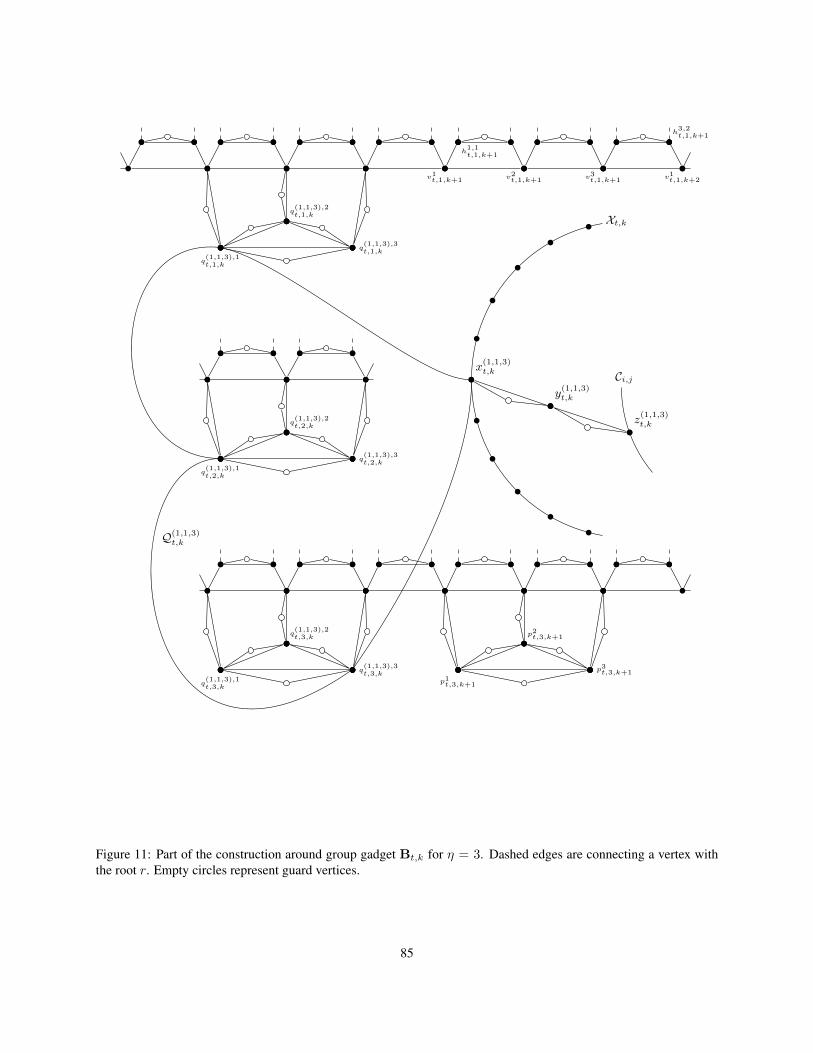
v1t,1,k+1 v2
t,1,k+1 v3t,1,k+1 v1
t,1,k+2
h1,1t,1,k+1
h3,2t,1,k+1
p1t,3,k+1
p2t,3,k+1
p3t,3,k+1
q(1,1,3),1t,1,k
q(1,1,3),2t,1,k
q(1,1,3),3t,1,k
q(1,1,3),1t,2,k
q(1,1,3),2t,2,k
q(1,1,3),3t,2,k
q(1,1,3),1t,3,k
q(1,1,3),2t,3,k
q(1,1,3),3t,3,k
Q(1,1,3)t,k
x(1,1,3)t,k
Xt,k
y(1,1,3)t,k
z(1,1,3)t,k
Ci,j
Figure 11: Part of the construction around group gadget Bt,k for η = 3. Dashed edges are connecting a vertex withthe root r. Empty circles represent guard vertices.
85

We can view the whole construction as a matrix of group gadgets, where each row corresponds to some group ofvariables Ft and each column is devoted to some clause in such a way that each clause gets (2ηn′+1) private columns(but not consecutive) of the group gadget matrix, as in Figure 12.
r
Bn′,0 Bn′,a−1
B1,0 B1,a−1
Ci,j
Figure 12: The arrangement of the group gadgets in G.
Finally, we define the size of the feedback vertex set we are looking for as K = Kh +Kv +Kp +Kq +Kx +Ky ,where
Kh = ηn′(3a− 1) Kv = ηn′a Kp = ηn′ · 2aKq = ηn′ · 2a3η Kx = n′a Ky = n′a3η.
Correctness
Lemma D.18. If Φ has a satisfying assignment, then there exists a feedback vertex set in G of size K.
Proof. Given a satisfying assignment φ of the formula Φ we construct a feedback vertex set X ⊆ V as follows.For each group of variables Ft we consider the sequence St ∈ 1, 2, 3η which corresponds to the restriction of
86

the assignment φ to the variables of Ft. Let
Xv = vSt(`)t,`,k : 1 ≤ t ≤ n′, 1 ≤ ` ≤ η, 0 ≤ k < aXp = pαt,`,k : 1 ≤ t ≤ n′, 1 ≤ ` ≤ η, 0 ≤ k < a, 1 ≤ α ≤ 3, α 6= St(`)Xq = qS,αt,`,k : 1 ≤ t ≤ n′, 1 ≤ ` ≤ η, 0 ≤ k < a, S ∈ 1, 2, 3η, 1 ≤ α ≤ 3, α 6= St(`)Xx = xStt,k : 1 ≤ t ≤ n′, 0 ≤ k < aXy = ySt,k : 1 ≤ t ≤ n′, 0 ≤ k < a, S ∈ 1, 2, 3η, S 6= StXz = zStt,k : 1 ≤ t ≤ n′, 0 ≤ k < a
Moreover, we define the set Xh ⊆ H to contain, for each 1 ≤ t ≤ n′, 1 ≤ ` ≤ η, 0 ≤ k < a, 1 ≤ α ≤ 3 and(k, α) 6= (a− 1, 3), the vertex hα,1t,`,k if vαt,`,k /∈ Xv and the vertex hα,2t,`,k otherwise. Note that |Xv| = Kv , |Xp| = Kp,|Xq| = Kq , |Xx| = Kx, |Xy|+ |Xz| = Ky and |Xh| = Kh. Thus a set X = Xv ∪Xp ∪Xq ∪Xx ∪Xy ∪Xz ∪Xh
is of size K.To finish the proof we need to verify that X is a feedback vertex set of G. First, we ensure that X includes at least
one endpoint of every triangle edge in G.
1. X includes one vertex from each pair hα,1t,`,k and hα,2t,`,k.
2. X includes two out of three vertices in each triple pαt,`,k, 1 ≤ α ≤ 3, and in each triple qS,αt,`,k, 1 ≤ α ≤ 3.
3. If pαt,`,k /∈ X or qS,αt,`,k /∈ X , then vαt,`,k ∈ X .
4. If ySt,k /∈ X then both xSt,k and zSt,k are in X .
Let G0 be the graph G with deleted guard vertices. We have just shown that each guard vertex in G \X is of degreezero or one. Thus if G0 \X is a forest, then G \X is a forest too.
Now note that Xp ∪Xq ∪Xv separates (r ∪V∪H) \X from the rest of the graph G0. To see this recall that ifpαt,`,k /∈ X or qS,αt,`,k /∈ X , then vαt,`,k ∈ X . Let G1 = G0[r ∪ V ∪H]. We now show that G1 \X is a forest. Notethat in G1 \Xh each cycle contains at least one vertex from V. Recall that the set Xv contains every third vertex oneach path Vt,`. Let vαt,`,k and vα
′t,`,k′ be any two consecutive vertices on Vt,` that are not in Xv . It is straightforward
to check that that in the set of at most 4 neighbours of these two vertices in H, at most one is not in Xh. Thus, thevertices in V \Xv do not take part in any cycle in G1 \X , and G1 \X is a forest.
Now note that Xv ∪Xq ∪Xx ∪Xy separates (Q ∪ X) \X from the rest of the graph G0. To see this recall that ifpαt,`,k /∈ X or qS,αt,`,k /∈ X , then vt,`,k ∈ X and if xSt,k /∈ X then ySt,k ∈ X . Let G2 = G0[Q ∪ X]. We now show thatG2 \X is a forest. The vertices in Q∪X from different group gadgets are not adjacent, thus we focus on a single groupgadget Bt,k. Let S ∈ 1, 2, 3η . Note that in G2 \X the vertices from QSt,k \X are of degree at most two, except for
the vertex xSt,k. If S 6= St, then for any 1 ≤ ` ≤ η such that S(`) 6= St(`) we have qS,S(`)t,`,k ∈ Xq and the cycle QSt,k
is intersected by X . On the other hand, if S = St, then xSt,k ∈ Xx. Thus, the vertices Q \X are not contained in anycycle in G2 \X . Moreover, on each cycle Xt,k we have xStt,k ∈ Xx and we infer that G2 \X is a forest.
As for Y, note that if ySt,k /∈ X then S = St and xSt,k, zSt,k ∈ X , and ySt,k is isolated in G0 \X .
We are left with Z. The graph G3 = G0[Z] consists of a cycles Ci,j , 0 ≤ i < m, 0 ≤ j < 2ηn′ + 1. Considera clause Ci and an index 0 ≤ j < 2ηn′ + 1. As φ satisfies Ci, there exists a block Ft, such that a variable from thisblock satisfies Ci. Then zStt,mi+j is both on the cycle Ci,j and in X , and G3 \X is a forest, too.
Lemma D.19. If there exists a feedback vertex set X of size at most K in the graph G, then Φ has a satisfyingassignment.
Proof. As it is discussed at the begining of the construction process, we may assume that no guard vertex is in X . LetXh = X ∩H, similarly we define Xv , Xp, Xq , Xx, Xy and Xz . Furthermore, we assume that, among all feedbackvertex sets of size at most K in G that do not contain any guard vertex, the set X is such a one that |Xp| is the smallestpossible.
We now lower bound the sizes of the sets Xh, Xv , Xp, Xq , Xx, Xy and Xz .
87
1. For each 1 ≤ t ≤ n′, 0 ≤ k < a, S ∈ 1, 2, 3η , at least one of the vertices ySt,k and zSt,k is in X (as they areconnected by a triangle edge), thus |Xy|+ |Xz| ≥ n′a3η = Ky .
2. For each 1 ≤ t ≤ n′ and 0 ≤ k < a at least one vertex of the set X needs to hit the cycle Xt,k, to |Xx| ≥ n′a =Kx.
3. For each 1 ≤ t ≤ n′, 0 ≤ k < a, 1 ≤ ` ≤ η and S ∈ 1, 2, 3η at least two vertices out of the tripleqS,αt,`,k : 1 ≤ α ≤ 3 need to be included in X , thus |Xq| ≥ ηn′ · 2a3η = Kq .
4. For each 1 ≤ t ≤ n′, 0 ≤ k < a, 1 ≤ ` ≤ η at least two vertices out of the triple pαt,`,k : 1 ≤ α ≤ 3 need tobe included in X . Moreover, if pαt,`,k /∈ X for some 1 ≤ α ≤ 3, then vαt,`,k ∈ X , as otherwise the triangle edgevαt,`,kp
αt,`,k is not covered by X . Thus |Xp|+ |Xv| ≥ ηn′ · 3a = Kp +Kv .
5. For each 1 ≤ t ≤ n′, 0 ≤ k < a, 1 ≤ ` ≤ η, 1 ≤ α ≤ 3, such that (k, α) 6= (a− 1, 3), at least one endpoint ofthe triangle edge hα,1t,`,kh
α,2t,`,k needs to be included in X . Thus |Xh| ≥ ηn′(3a− 1) = Kh.
As |X| ≤ K = Kh +Kv +Kp +Kq +Kx +Ky , we infer that in all aforementioned inequalities we have equalities,and r /∈ X .
Recall that we have assumed that |Xp| is the smallest possible. Let 1 ≤ t ≤ n′, 0 ≤ k < a, 1 ≤ ` ≤ η and focuson the triple pαt,`,k : 1 ≤ α ≤ 3. If it is wholy contained in X , then X \ p1
t,`,k ∪ v1t,`,k is also a feedback vertex
set of G, of not greater size, not containing any guard vertex, and with smaller size of |Xp|. Thus X contains exactlytwo vertices out of each such triple, |Xp| = Kp, |Xv| = Kv and Xv contains exactly one vertex out of each triplevαt,`,k : 1 ≤ α ≤ 3.
We strengthen the above observation by showing the following claim: for any 1 ≤ t ≤ n′, 1 ≤ ` ≤ η and anythree consecutive vertices vA, vB , vC on the path
⋃a−1k=0 Vt,`,k, at least one of these vertices is inXv . By contradiction,
assume that vA, vB , vC /∈ X . Recall that the graph G contains vertices h1A, h2
A, h1B , h2
B , edges rh1A, rh2
A, rh1B , rh2
B ,h1AvA, h2
AvB , h1BvB , h2
BvC and triangle edges h1Ah
2A, h1
Bh2B . Note that |h1
A, h2A, h
1B , h
2B \X| = 2, as |Xh| = Kh
andXh contains exactly one vertex from each pair connected by a triangle edge. These two vertices in H\X , togetherwith vA, vB , vC and the root r induce a subgraph of G \X with 6 vertices and 6 edges, a contradiction.
For 1 ≤ t ≤ n′ and 1 ≤ ` ≤ η let us define a sequence st,`(k), 0 ≤ k < a, such that vαt,`,k ∈ Xv iff α = st,`(k).By the observation made in the previous paragraph we infer that the sequence st,` cannot increase, thus its valuecan change at most twice. As a = m(2ηn′ + 1), we infer that there exists an index 0 ≤ j < 2ηn′ + 1 such thatfor all 1 ≤ t ≤ n′, 1 ≤ ` ≤ η we have st,`(mj) = st,`(mj + i) for all 0 ≤ i < m. For each block Ft, letSt = (st,`(mj))
η`=1 ∈ 1, 2, 3η and let φ be an assignment that corresponds to the sequence St for each block Ft.
We claim that φ satisfies Φ.Take any clause Ci, 0 ≤ i < m. Take any block Ft. As |Xq| = Kq , the set Xq includes exactly two vertices out
of each triple qS,αt,`,mj+i : 1 ≤ α ≤ 3 for 1 ≤ ` ≤ η, S ∈ 1, 2, 3η . As qS,αt,`,mj+i is connected to vαt,`,mj+i by atriangle edge, we infer that qS,αt,`,mj+i /∈ X iff vαt,`,mj+i ∈ X , which is equivalent to St(`) = α. Thus xStt,mj+i ∈ X ,as otherwise the cycle QStt,mj+i is disjoint with X . As |Xx| = Kx, the set Xx contains exactly one vertex out of eachcycle Xt,k, and we infer that xSt,mj+i /∈ X for S 6= St. Recall that xSt,mj+i and ySt,mj+i are connected by a triangleedge, thus ySt,mj+i ∈ X for S 6= St. As |Xy|+ |Xz| = Ky , we know that the set X contains exactly one endpoint outof each triangle edge ySt,mj+iz
St,mj+i, and we infer that if zSt,mj+i ∈ X then S = St. Finally, if X is a feedback vertex
set in G, X hits the cycle Ci,j , thus there exists a block Ft and a sequence S ∈ 1, 2, 3, η such that zSt,mj+i ∈ Xand the assignment of the variables of the block Ft that corresponds to S satisfies Ci. However, we have proven thatzSt,mj+i ∈ X implies S = St, thus φ satisfies Ci and the proof is finished.
Pathwidth bound
Lemma D.20. Pathwidth of the graph G is at most ηn′ +O(η3η). Moreover a path decomposition of such width canfound in polynomial time.
Proof. We give a mixed search strategy to clean the graph with ηn′+O(η3η) searchers. First we put a searcher in theroot r. This searcher remains there till the end of the cleaning process.
88

For a gadget Bt,k we call the vertices v1t,`,k for 1 ≤ ` ≤ η, as entry vertices. We search the graph in a =
m(2ηn′ + 1) rounds. In the beginning of round k (0 ≤ k < a) there are searchers on the entry vertices of the gadgetBt,k for every 1 ≤ t ≤ n′. Let 0 ≤ i < m and 0 ≤ j < 2ηn′ + 1 be integers such that k = i + mj. We place asearcher on the last vertex of the cycle Ci,j (recall that the vertices on Ci,j are sorted by the block number). Then, foreach 1 ≤ t ≤ n′ in turn we:
• put O(η3η) searchers on all vertices of the group gadget Bt,k,
• put η searchers on entry vertices of the group gadget Bt,k+1 (except for the last round),
• put a searcher in the first vertex after the vertices of Bt,k ∩ Z on the cycle Ci,j ,
• remove searchers from all vertices of the group gadget Bt,k.
The last step of the round is removing the remaining searcher on the cycle Ci,j . After the last round the whole graphG is cleaned. Since we reuse O(η3η) searchers for cleaning group gadgets, ηn′ + O(η3η) searchers suffice to cleanthe graph.
Using the above graph cleaning process a path decomposition of width ηn′ +O(η3η) can be constructed in poly-nomial time.
Proof of Theorem D.17. Suppose FEEDBACK VERTEX SET can be solved in (3−ε)p|V |O(1) time provided that we aregiven a path decomposition of G of width p. Let λ = log3(3− ε) < 1. We choose η large enough such that log 3η
blog 3ηc <1λ . Given an instance of SAT we construct an instance of FEEDBACK VERTEX SET using the above construction andthe chosen value of η. Next we solve FEEDBACK VERTEX SET using the 3λp|V |O(1) time algorithm. Lemmata D.18,D.19 ensure correctness, whereas Lemma D.20 implies that running time of our algorithm is 3ληn
′ |V |O(1), howeverwe have
3ληn′
= 2ληn′ log 3 = 2λn
′ log 3η ≤ 2C · 2λn log 3η/blog 3ηc = 2C · 2λ′n
for some λ′ < 1 and C = λ log 3η . This concludes the proof.
89