Exponential-Family Random Graph Models with Time Varying Network

Parameters

Abstract

Dynamic networks are a general language for describing time-evolving complex systems, and have long been

an interesting research area. It is a fundamental research question to model time varying network parameters.

However, due to difficulties in modeling functional network parameters, there is little progress in the current

literature to effectively model time varying network parameters. In this work, we consider the situation in which

network parameters are univariate nonparametric functions instead of constants. Using a kernel regression

techniques, we introduce a novel unified procedure to effectively estimate those functional network parameters

in the exponential-family random graph models. Moreover, by adopting the finite mixture models, we extend

our model to mixture of exponential-family random graph models with functional network parameters which

simultaneously allows both modeling and detecting communities for the dynamic networks. To choose optimal

number of communities and kernel bandwidth, we propose conditional likelihood BIC and choose bandwidth

by adopting the idea of network cross validation. Furthermore, we design an efficient variational expectation-

maximization algorithm to find approximate maximum local likelihood estimates of network parameters and

global estimates of mixing proportions. The power of our method is demonstrated in depth simulation studies

and real-world applications to dynamic arm trade networks.

Keywords. Dynamic networks, Exponential-family random graph model (ERGM), Functional network pa-

rameter, Variational EM algorithm, Minorization-maximization, Model selection, Arm trade networks.

1

1 Introduction

Dynamic networks are a general language for describing time-evolving complex systems, and have long been an

interesting research area. Recently, due to advances in data collection technologies, larger-scale and longer time

span dynamic network analysis has been increasingly important in various research fields such as sociology,

business, finance, bioinformatics, genomics, physics, artificial intelligence, and many others. In the current

literature, to handle networks that change over time, many works are done under Markov assumption. The

idea of dynamic Markovian models of network starts from modeling social network dynamics. Holland & Lein-

hardt (1977) proposed continuous-time Markov process and Wasserman (1979, 1980) continued and provided

estimators for various parametric models. Later, Leenders (1995) studied maximum likelihood estimation

for continuous-time Markov process models based on the assumptions that dyad processes are independent

and stationary. Snijders (2001) relaxed assumptions of previous models and introduced parameterizations of

continuous-time Markov processes that allow dyad processes to be dependent and less restrictive stationarity

assumption.

More recently, the exponential-family random graph modeling (ERGM) framework has become a popular

approach for conducting inference on network structure, due to its generalizability (Frank & Strauss 1986,

Strauss & Ikeda 1990, Wasserman & Pattison 1996, Robins & Pattison 2001, Snijders et al. 2006, Hunter et al.

2008). Exponential family random graph models allow researchers to incorporate interesting features of the

network into statistical models. For many years, the application of the ERGM framework was limited to static

network datasets. However, recent developments have extended ERGMs to the modeling of dynamic networks

under discrete-time Markov models as alternatives to continuous-time Markov models. Hanneke et al. (2010)

proposed a temporal ERGM (TERGM) to fit the model to a network series and Krivitsky & Handcock (2014)

proposed a separable temporal ERGM (STERGM) that gives more flexibility in modeling dynamic networks.

Several works are also done in non-Markovian approach to model dynamic networks. Butts (2008) developed

a relational event framework based on survival analysis theory. Hunter et al. (2011) continued this approach

and used multivariate counting processes to model network dynamics. They focused on dynamic egocentric

framework and used multivariate counting process to every node to model continuous-time network data.

Similarly, Perry & Wolfe (2013) used multivariate counting process to every pair of nodes which is also known

as dynamic relational framework.

In this work, we consider the situation in which network parameters are univariate nonparametric functions

instead of constants. Using a kernel regression techniques, we introduce a novel unified procedure to effectively

estimate those functional network parameters in the exponential-family random graph models. Moreover, by

adopting the finite mixture models, we extend our model to mixture of exponential-family random graph models

with functional network parameters which simultaneously allows both modeling and detecting communities for

the dynamic networks.

In Section 2, we first present exponential-family random graph model with functional network parameters.

We also extend our model to mixture of exponential-family random graph models with functional network

2

parameters by adopting the finite mixture models. Section 3 designs an efficient variational expectation-

maximization algorithm to find approximate maximum local likelihood estimates of network parameters and

global estimates of mixing proportions. Given these estimates, we can further infer membership labels and

solve the problem of community detection for dynamic networks. In Section 4, we first choose optimal number

of communities using conditional likelihood BIC and choose kernel bandwidth by adopting the idea of network

cross validation. The power of our method is demonstrated by simulation studies in Section 5 and real-world

application to dynamic arm trade networks in Section 6.

2 Exponential-family Random Graph Models with Time Varying

Network Parameters: A Semiparametric Approach

In this section, we present the mixture of exponential-family random graph models with functional network

parameters. First we introduce some necessary notation. Let Yt = (Yt,ij)1≤i 6=j≤n ∈ Y represent the network

at time t and denote by yt = (yt,ij)1≤i 6=j≤n the corresponding observed network at time t. Define Y as the set

of all possible networks.

2.1 Exponential-family random graph model with functional network parameters

Let θ(·) be the functional network parameters of interest. Given some univariate covariate ut, exponential-

family random graph model with functional network parameters is written as follows:

Pθ(ut)(Yt = yt) = exp{θ(ut)′g(yt)− ψ(θ(ut))}. (1)

where ψ(θ(ut)) = log∑

y∗t∈Yexp [θ(ut)

′g(y∗t )] .

Here g(yt) is the p-dimensional sufficient statistic from network yt and C(θ(ut)) = exp{ψ(θ(ut))} is the nor-

malization term. However, the model in (1) is not scalable for modeling large networks. To make exponential-

family distributions scalable, dyadic independence is usually used in the specification of ERGMs.

Therefore, we focus on scalable exponential-family random graph models, which are characterized by fol-

lowing dyadic independence,

Pθ(ut)(Yt = yt) =

n∏i<j

Pθ(ut)(Dt,ij = d), (2)

where Dt,ij corresponds to Yt,ij in the case of undirected edges and (Yt,ij , Yt,ji) in the case of directed edges.

The subscribed i < j and superscripted n mean that the product in (2) should be taken over all pairs (i, j)

with 1 ≤ i < j ≤ n.

Dyadic independence has at least two advantages: (a) it facilities estimation, because the computing time to

evaluate the likelihood function scales linearly with n2; (b) by design it bypasses the so-called model degeneracy

problem: if n is large, some exponential family models without dyadic independence then to be ill-defined and

impractical for modeling networks (Strauss 1986, Handcock et al. 2003, Schweinberger 2011, Vu et al. 2013).

3

In this paper, we focus on scalable exponential-family models by assuming the the dyadic independence.

2.2 Mixture of exponential-family random graph models with functional network

parameters

Most exponential families with dyadic independence are either simplistic or nonparsimonius (model with O(n)

parameters) (Vu et al. 2013). We therefore adopt the finite mixture model, which offer powerful statistical

techniques to identify subpopulations with certain commonality within overall population.

Define Z = (Z1, . . . , Zn) as the membership vector, where Z1, . . . , Zn ∈ {1, . . . ,K}. Denote by K the

number of communities. Assume that Zi’s are independently drawn from a multinomial distribution with

parameter π = (π1, . . . , πK), where πk > 0 for all k. We therefore assume that the probability mass function

has a K-component mixture form as follows:

Pπ,θ(ut)(Yt = yt) =∑

z∈{1,...,K}nPθ(ut)(Yt = yt|z)Pπ(Z = z) (3)

Here we extend dyadic independence to conditional dyadic independence given the community structure of

networks as follows:

Pθ(ut)(Yt = yt|z) =

n∏i<j

Pθzizj (ut)(Dt,ij = d|z). (4)

Given (4), the probability mass function of K-component mixture is written as follows:

Pπ,θ(ut)(Yt = yt) =∑

z∈{1,...,K}n

n∏i<j

Pθzizj (ut)(Dt,ij = d|z)Pπ(Z = z) (5)

Now, given the independent data {(yt, ut), 1 ≤ t ≤ T} our goal is to estimate π’s and nonparametric

function θ(·)’s. The log-likelihood function for the observed data is given by

` =

T∑t=1

log[Pπ,θ(ut)(Yt = yt)

]=

T∑t=1

log

∑z∈{1,...,K}n

Pθ(ut)(Yt = yt|z)Pπ(Z = z)

(6)

Since θ(·) is nonparametric, we need nonparametric smoothing techniques for (6). Here we employ kernel

regression techniques. In kernel regression, we first use local constants θu to approximate θ(u). Let Kh(·) =

h−1K(·/h) be a rescaled kernel of a kernel function K(·) with a bandwidth h. Then the corresponding local

log-likelihood function for observed data is

`u =

T∑t=1

log

∑z∈{1,...,K}n

Pθu(Yt = yt|z)Pπ(Z = z)

Kh(ut − u) (7)

4

Thus our aim is first solve parameter π via maximizing the log-likelihood `,

π = arg maxπ

`(π,θ(u))

and solve local network parameters θu via maximizing the local log-likelihood `u, namely

θu = arg maxθu

`u(π,θu)

Before proceeding we give specific examples of undirected and directed network models.

Example 1: Undirected Network Model

Here we introduce one parameter: (a) edge (density) parameter, θe. There are two possible values 1 and 0.

The probabilities for two possible values of each dyad are given as follows:

1. Pθe(ut)(Dt,ij = 1|zi = k, zj = l) = exp(θek(ut) + θel (ut)− ψ(θe(ut)))

2. Pθe(ut)(Dt,ij = 0|zi = k, zj = l) = exp(−ψ(θe(ut)))

where ψ(θe(ut)) = log(1 + exp(θek(ut) + θel (ut))).

Example 2: Directed Network Model with Outgoing-edge and Reciprocity Parameters

Here, we introduce two parameters: (a) outgoing-edge parameter, θoe and (b) reciprocity parameter, θre.

There are four possible values, (1, 1), (1, 0), (0, 1) and (0, 0). The probabilities for all possible values of each

dyad are given as follows:

1. Pθ(ut)(Dt,ij = (1, 1)|zi = k, zj = l) = exp(θrek (ut) + θrel (ut)− ψ(θ(ut)))

2. Pθ(ut)(Dt,ij = (1, 0)|zi = k, zj = l) = exp(θoek (ut)− ψ(θ(ut)))

3. Pθ(ut)(Dt,ij = (0, 1)|zi = k, zj = l) = exp(θoel (ut)− ψ(θ(ut)))

4. Pθ(ut)(Dt,ij = (0, 0)|zi = k, zj = l) = exp(−ψ(θ(ut)))

where ψ(θ(ut)) = log(1 + exp(θrek (ut) + θrel (ut)) + exp(θoek (ut)) + exp(θoel (ut))).

2.3 Parameter identifiability

Lemma 1. (Allman et al. 2011, Theorem 14) The parameters of the random graph mixture model, with κ-state

edge variables and K ≥ 2 latent groups, are identifiable, up to label switching, from the distribution of K9,

provided κ ≥ (K+1)K2 and the κ-entry vectors {pkl}1≤k≤l≤K are linearly independent.

Assumption 1. We assume that for any u, the K values {θuk , 1 ≤ k ≤ K} are distinct.

Theorem 1. Under the condition of Lemma 1 and with fixed community membership, mixing proportion

parameter {πk : 1 ≤ k ≤ K} is identifiable up to label switching and local network parameters {θu : ∀u ∈ U}

are identifiable up to global label switching.

5

3 Effective Variational EM algorithm

For a given u, one may maximize the local log-likelihood function (7) using an variational EM algorithm.

However, in practice we typically want to evaluate the unknown functions at a set of grid points. This requires

us to maximize the local likelihood function (7) at different grid points. This imposes some challenges because

the labels in the variational EM algorithm may change at different grid points. Thus a naive implementation

of the variational EM algorithm may fail to yield smooth estimated curves. The key idea is that given current

estimates of parameters, π and θ(·), E-step estimates variational parameter at observed u1, . . . , uT and M-step

uses the obtained common variational parameter estimate to update all estimates of network parameters at

each grid point. Hence, we effectively prevent the label switching issue at different grid points.

3.1 Variational E-step

Using Jensen’s inequality, log-likelihood function is bounded from the below as follows:

`(π,θ(ut)) =

T∑t=1

log

[∑z∈Z

Pπ,θ(ut)(Yt = yt,Z = z)

A(z)A(z)

]

≥T∑t=1

∑z∈Z

[log

Pπ,θ(ut)(Yt = yt,Z = z)

A(z)

]A(z)

=

T∑t=1

[EA(logPπ,θ(ut)(Yt = yt,Z = z))− EA(logA(z))

]Let Γ = (γ1, . . . ,γn)′ be the variational parameter, which denotes the mixed membership of nodes where Γ

is (n×K) matrix and {γi, i = 1, . . . , n} are (K × 1) vectors. Let Pγi(Zi = zi) be Multinomial (1; γi1, . . . , γiK)

for i = 1, 2, . . . , n. A natural subset of tractable choices is given by setting,

A(z) = Pγ(Z = z) =

n∏i=1

Pγi(Zi = zi)

Now we can write our effective lower bound as follows:

ELBO(π,θ(ut); Γ) =

T∑t=1

n∑i<j

K∑k=1

K∑l=1

γikγjl logPθ(ut)(Dt,ij = d|z)

+ T

[n∑i=1

K∑k=1

γik(log πk − log γik)

]

Let Γ, π, θ(·) be the current estimate. In the E-step our goal is to find updates, γnewik by solving the

following univariate optimization problem:

γnewik ⇐ arg maxγik

{ELBO(γik; γi′k′ = γi′k′ , (i′, k′) 6= (i, k), π, θ(·))}

6

We can write our lower bound with respect to γi for i = 1, . . . , n− 1 given all other current estimates,

ELBO(γi;γj = γj , j > i, π, θ(·)) =

T∑t=1

n∑j=i+1

K∑k=1

K∑l=1

γikγjl logPθ(ut)(Dt,ij = d|z)

+ T

[K∑k=1

γik(log πk − log γik)

] (8)

and for γn,

ELBO(γn; π) = T

[K∑k=1

γnk(log πk − log γnk)

]. (9)

However, to solve the above optimization problem we have to solve non-convex optimization problem. To

make computationally attractive, we introduce Q(γi; Γ, π, θ(·)) which is a minorization function of the lower

bound (8) and (9).

Here we consider following minorization function. For i = 1, . . . , n− 1,

Q(γi; Γ, π, θ(·)) =

T∑t=1

n∑j=i+1

K∑k=1

K∑l=1

(γ2ik

γjl2γik

+γjlγik

2

)logPθ(ut)

(Dt,ij = d|z)

+ T

[K∑k=1

γik(log πk − log γik −γikγik

+ 1)

].

and for i = n,

Q(γn; Γ, π) = T

[K∑k=1

γnk(log πk − log γnk −γnkγnk

+ 1)

].

Note that Q(γi; Γ, π, θ(·)) is a concave function, and we can maximize Q(γi; Γ, π, θ(·)) solving a constrained

quadratic programming problems, under constraints γi1, . . . , γiK ≥ 0 and∑Kk=1 γik = 1 for i = 1, · · · , n.

3.2 Variational M-step

In the variational M-step, maximization with respect to π and θu may be accomplished separately. First, to

derive the closed-from updates for π, we maximize following lower bound via introducing Lagrange multiplier

with the constraint∑Kk=1 πk = 1.

ELBO(π; θ(u), Γ) =

T∑t=1

n∑i<j

K∑k=1

K∑l=1

γikγjl logPθ(u)(Dt,ij = d|z)

+ T

[n∑i=1

K∑k=1

γik(log πk − log γik)

].

(10)

Then it is easy to obtain the closed-form update for π, that is

πnewk =

1

n

n∑i=1

γik, k = 1, . . . ,K. (11)

Next to update θu, we maximize following local lower bound using Newton-Raphson method with the

7

gradient and Hessian of (12).

ELBO(θu; π, Γ) =

T∑t=1

n∑i<j

K∑k=1

K∑l=1

γikγjl logPθu(Dt,ij = d|z)

Kh(ut − u)

+

T∑t=1

[n∑i=1

K∑k=1

γik(log πk − log γik)

]Kh(ut − u).

(12)

The successor point θu(new) is given by

θu(new) = θu −H(θu)−1∇ELBO(θu; π, Γ). (13)

3.3 Ascent property of ELBO

We can show that our variational EM algorithm preserves ascent property of lower bound of the log-likelihood,

which leads the best estimates of lower bound. In Variational E-step, we maximize our lower bound with

respect to variational parameters through MM algorithm via introducing surrogate function to minorize the

lower bound which satisfy following equations,

Q(γi; Γ, π, θu) ≤ ELBO(γi;γj = γj , j > i, π, θu),

Q(γi; Γ, π, θu) = ELBO(γi;γj = γj , j > i, π, θu),

for all i = 1, . . . , n. Therefore using above equations we have,

ELBO(γi;γj = γj , j > i, π, θu) ≤ Q(γ(new)i ; Γ, π, θu)

≤ ELBO(γ(new)i ;γj = γj , j > i, π, θu),

for i = 1, . . . , n. In Variational M-step, we maximize our local lower bound with respect to network parameters

which leads,

ELBO(π, θu; γ(new)) ≤ ELBO(π(new), θu(new); γ(new)).

Therefore, we prove the ascent property of local lower bound of the log-likelihood,

4 Model Selection

In practice, it is important to effectively choose the number of communities. To determine number of communi-

ties K, we consider the information criterion approach. Bayesian Information Criterion (BIC) has the general

form of −2L + δ × df, where L is the maximum log-likelihood, δ = logN , and df is the degree of freedom to

measure model complexity.

Here, we use the conditional likelihood of the network series, conditioning on an estimate of the membership

vector, to construct an effective model selection criterion.

8

We obtain the conditional log-likelihood of the network series y1,y2, . . . ,yT given estimated membership

vector as

cl(θ(·), z) =

T∑t=1

log(Pθ(ut)(Yt = yt|z)

), (14)

which can be written using conditional dyadic independence (4) in the form

cl(θ(·), z) =

T∑t=1

∑i<j

log(Pθzizj (ut)(Dt,ij = d|z)

).

Next, to specify the degree of freedom in (3), we follow Fan et al. (2001) and Huang et al. (2013) to derive

the degree of freedom. Denote by df = τKh−1|Z|

(K(0)− 1

2

∫K2(t) dt

)the degree of freedom of a univariate

nonparametric function, where Z is the support of the covariate Z, and τK =K(0)− 1

2

∫K2(t) dt∫

(K(t)− 12K∗K(t))

2dt. Hence, for

each pair of (K,h), the conditional likelihood BIC is defined as

clBIC(K,h) = −2cl(θ(·)mle, z) + log(T (n(n− 1)/2)) · df(K,h),

where df(K,h) = tr(H−1K VK) · df approximates the degrees of freedom based on HK = E(−∇2θ(·)cl(θ(·), z))

and VK = Var(∇θ(·)cl(θ(·), z)). We first select optimal K by minimizing the clBIC score, and then choose h

by network cross-validation (NCV). We choose K by minimizing the best available clBIC score for each choice

of K over different choices of h, Namely,

K = arg min(K,h)

clBIC(K, h)

After fixing K = K, we use negative conditional log-likelihood to construct loss, and choose bandwidth h by

NCV. We follow Chen and Lei (2016) to describe the V -fold dynamic network cross-validation procedure. We

summarize the details in Algorithm 1. We follow Chen & Lei (to appear) to perform NCV multiple times with

independent V -fold splits and output the most frequent h. We used V = 3 and twenty repetitions.

5 Simulation Studies

In this section, we conduct two simulation studies. Section 5.1 considers ERGM with functional network param-

eters, while Section 5.2 considers mixture of ERGMs with functional network parameters. Before proceeding,

we first introduce the common simulation setting and two measurements to compare numerical performances.

We assume the dynamic network data are observed at equally spaced 51 discrete time points, with node size

100. Here, we introduce several average metrics over 100 replications.

First, to assess the performance of the estimator of the network parameter function, we consider the square

9

Algorithm 1 V -fold dynamic networks cross-validation

Input: adjacency matrices, Y1,Y2, . . . ,YT , a set of candidate values for h, number of folds V ≥ 2.

1. Block-wise node-pair splitting:

Randomly split the nodes into V equal-sized subsets {Nv : 1 ≤ v ≤ V }, and split the adjacency matricescorresponding into V × V equal sized blocks for t = 1, . . . , T ,

Yt = (Y(uv)t : 1 ≤ u, v ≤ V ),

where Y(uv)t is the submatrix of Yt with rows in Nu and columns in Nv

2. For each 1 ≤ v ≤ V , and each h

• Estimation: Estimate functional network parameters θ(·) and membership vector z using the subma-

trix, Y(−vv)t obtained by removing the Y

(vv)t in subset Nv for all t = 1, . . . , T ,

• Validation: Calculate the predictive loss evaluated on Y(vv)t . For the loss function `, we use negative

conditional log-likelihood.

L(v)

(Y1, . . . ,Yt, h) =T∑t=1

∑i,j∈Nv ,i<j

`(Dt,ij , θtzizj

)

3. Let L(Y1, . . . ,YT , h) =∑V

v=1 L(v)

(Y1, . . . ,YT , h).

Output:h = arg min

hL(Y1, . . . ,YT , h)

root of the average squared error (RASE) of estimator of the function,

RASEθ =

√√√√ 1

G

∑u∈U

K∑k=1

(θuk − θuk

)2,

where G is the number of grid points.

Next, to assess the clustering performance, we calculate the Rand Index (RI) (Rand 1971). The measure

RI(z, z) calculates the proportion of pairs whose estimated labels correspond to the true labels in terms of

being assigned to the same or different groups:

RI(z, z) =1(n2

) ∑i<j

(I{zi = zj}I{zi = zj}+ I{zi 6= zj}I{zi 6= zj}).

5.1 ERGM with functional network parameters

In this section, we conduct simulation for exponential-family random graph model with functional network

parameter. Model 1 is directed network with functional out-going edge parameter and functional reciprocity

parameter, θoe1 (u) = 1− sin(2πu) and θre1 (u) = cos(3πu)− 1, i.e., Example 2.

To simulate directed dynamic networks, we generate all the dyads between two nodes at each time point

from probabilities with specified functional network parameters in Model 1.

10

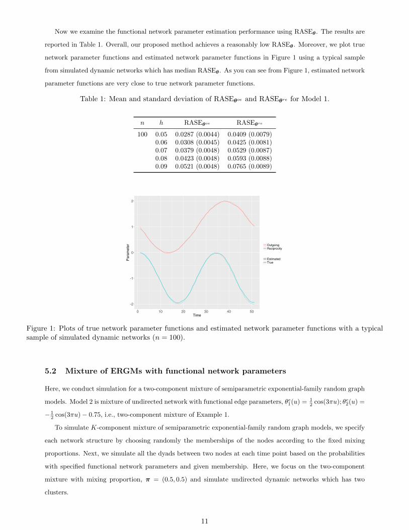
Now we examine the functional network parameter estimation performance using RASEθ. The results are

reported in Table 1. Overall, our proposed method achieves a reasonably low RASEθ. Moreover, we plot true

network parameter functions and estimated network parameter functions in Figure 1 using a typical sample

from simulated dynamic networks which has median RASEθ. As you can see from Figure 1, estimated network

parameter functions are very close to true network parameter functions.

Table 1: Mean and standard deviation of RASEθoe and RASEθre for Model 1.

n h RASEθoe RASEθre

100 0.05 0.0287 (0.0044) 0.0409 (0.0079)0.06 0.0308 (0.0045) 0.0425 (0.0081)0.07 0.0379 (0.0048) 0.0529 (0.0087)0.08 0.0423 (0.0048) 0.0593 (0.0088)0.09 0.0521 (0.0048) 0.0765 (0.0089)

-2

-1

0

1

2

0 10 20 30 40 50Time

Parameter Outgoing

Reciprocity

EstimatedTrue

Figure 1: Plots of true network parameter functions and estimated network parameter functions with a typicalsample of simulated dynamic networks (n = 100).

5.2 Mixture of ERGMs with functional network parameters

Here, we conduct simulation for a two-component mixture of semiparametric exponential-family random graph

models. Model 2 is mixture of undirected network with functional edge parameters, θe1(u) = 12 cos(3πu); θe2(u) =

− 12 cos(3πu)− 0.75, i.e., two-component mixture of Example 1.

To simulate K-component mixture of semiparametric exponential-family random graph models, we specify

each network structure by choosing randomly the memberships of the nodes according to the fixed mixing

proportions. Next, we simulate all the dyads between two nodes at each time point based on the probabilities

with specified functional network parameters and given membership. Here, we focus on the two-component

mixture with mixing proportion, π = (0.5, 0.5) and simulate undirected dynamic networks which has two

clusters.

11

We first check the performance of algorithm at identifying the correct number of communities. For given

bandwidth h, we count the frequencies of selected K’s over 100 repeats. For each simulated dynamic network

data, we should select K by minimizing the clBIC score over the four K’s and five bandwidths. The frequencies

of such selected K’s over 100 repeats are presented in the last column of Table 2. As shown in Table 2, our

proposed clBIC criterion based on min clBIC has a convincing performance of choosing correct number of

communities.

Table 2: Frequencies of selected K’s by clBIC for Model 2.

n h = 0.05 h = 0.06 h = 0.07 h = 0.08 h = 0.09 minh clBIC

100 K = 1 0 0 0 0 0 0K = 2 87 85 84 83 84 83K = 3 12 14 15 16 9 16K = 4 1 1 1 1 0 1

The average Rand Index results are reported in Table 3 and we achieve a high average Rand Index for

the correct number of mixtures. When K = 1, all nodes are clustered into the same community and so the

Rand Index only depends on the true labels. The results of Table 2 and 3 together tell us that our algorithm

based on conditional likelihood BIC performs convincingly in choosing the correct number of communities and

assigning nodes to communities.

Table 3: Mean and standard deviation of Rand Index for Model 2.

n h K = 1 K = 2 K = 3 K = 4

100 0.05 0.4993 (0.0067) 0.9791 (0.0130) 0.8870 (0.0380) 0.8299 (0.0466)0.06 0.4993 (0.0067) 0.9793 (0.0128) 0.8870 (0.0379) 0.8299 (0.0465)0.07 0.4993 (0.0067) 0.9791 (0.0130) 0.8870 (0.0379) 0.8298 (0.0467)0.08 0.4993 (0.0067) 0.9791 (0.0130) 0.8870 (0.0379) 0.8296 (0.0466)0.09 0.4993 (0.0067) 0.9789 (0.0128) 0.8867 (0.0378) 0.8294 (0.0463)

Next, we examine the functional network parameter estimation performance using RASEθe . The results

are reported in Table 4. Our proposed method achieves a reasonably low RASEθe . In this simulation, both

estimation and selection performances of our proposed method is not sensitive to bandwidths.

Table 4: Mean and standard deviation of RASEθe for Model 2.

n h RASEθe

100 0.05 0.1851 (0.0185)0.06 0.1862 (0.0185)0.07 0.1907 (0.0183)0.08 0.1930 (0.0182)0.09 0.1988 (0.0180)

12

6 Arm Trade Data

In real application, we use a data from the Stockholm International Peace Research Institute (SIPRI) Arms

Transfers Database which contains information on all transfers of major conventional weapons from 1950.

Here we focus on yearly arm trade networks from 1994 to 2013. To define networks, we first define edges as

follows: for any t = 1994, . . . , 2013, yt,ij = 1 if the volume of international transfers of arms, measured by trend

indicator value (TIV) from country i to country j in year t exceeds 1 million dollar in year t, and yt,ij = 0

otherwise. Next, to define the nodes in the networks, we choose the countries that satisfy above edge criterion

at least three times from 1994 to 2013. By using this criterion, among 198 existing countries, 145 countries

are remaining in the networks. Now, we model the arm trade networks employing mixture of semiparametric

ERGMs with out-going edge parameter and reciprocity parameter, i.e., K-component mixture of Example 2.

We use our proposed clBIC to determine the number of communities and K = 4 is chosen, which implies

four communities of countries with different functional out-going edge parameter and reciprocity parameter.

Next we use NCV to choose bandwidth and h = 0.25 is chosen.

In Figure 2, we plot the estimate out-going edge parameter and reciprocity parameter functions for each

community and in Figure 3 we choose four specific years and plot arm trade networks with estimated commu-

nities. As you can see from Figure 2, there are overall decreasing trend in arm trades until early 2000, however

after that there are overall increasing trends. Countries in community K3 show decreasing trend after 2004,

while countries in community K1 and K2 show slight decreasing trend after 2010. Countries in community K4

have most arm trades among all communities, while countries in K3 have least arm trades, which appear as

isolated nodes in Figure 3. Countries in K1 and K2 show similar trends but in different scale. Countries in K1

have slightly more arm trades than countries in K2.

-5.0

-4.6

-4.2

5 10 15 20Time

K1 oe

re

-6.3

-6.0

-5.7

-5.4

5 10 15 20Time

K3 oe

re

-5.75

-5.50

-5.25

-5.00

-4.75

5 10 15 20Time

K2 oe

re

-2.0

-1.5

-1.0

5 10 15 20Time

K4 oe

re

Figure 2: Estimated out-going edge parameter and reciprocity parameter functions for each community

13

1994Afghanistan

Austria

Lithuania

Luxembourg

Macedonia (FYROM)

Malaysia

MaldivesMali

Malta

Azerbaijan

Mauritania

Mauritius

Mexico

Moldova Mongolia

Morocco

MyanmarNamibia

Nepal

Netherlands

New Zealand

Niger

Nigeria

Norway

Bahrain

Oman

Pakistan

Panama

Paraguay

Peru

Philippines

Poland

Portugal

Bangladesh

Qatar

Romania

Russia

Rwanda

Barbados

Saudi Arabia

Senegal

Serbia

Seychelles

Sierra Leone

Singapore

Slovakia

Slovenia

Belarus

South Africa

Spain

Sri Lanka

Sudan

Suriname

Sweden

Switzerland

Syria

Belgium

Tajikistan

Tanzania

Thailand

Togo

Trinidad and Tobago

Tunisia

Turkey

Turkmenistan

Uganda

Ukraine

United Arab Emirates

United KingdomUnited States

Uruguay

Uzbekistan

Venezuela

Benin

Viet Nam

Yemen

Zambia

Zimbabwe

Albania

Bolivia

Bosnia and Herzegovina

Botswana

Brazil

Brunei Darussalam

Bulgaria

Burkina Faso

Burundi

CambodiaAlgeriaCameroon

Canada

Cape Verde

Chad

Chile

China

Colombia

DR Congo

Congo

Cote dIvoire

Croatia

Cyprus

Czech Republic

Denmark

Djibouti

Angola

Dominican RepublicEcuador

Egypt

El Salvador

Equatorial Guinea

Eritrea

Estonia

Ethiopia

Finland

France

Gabon

Georgia

Germany

Ghana

Greece

Argentina

Guinea

Hungary

India

Indonesia

Iran

Armenia

Iraq

Ireland

Israel

Italy

Jamaica

Japan

Jordan

Kazakhstan

Kenya

Australia

North Korea

South Korea

Kuwait

Kyrgyzstan

Laos

Latvia Lebanon

Libya

2000Afghanistan

Austria

Lithuania

Luxembourg

Macedonia (FYROM)

Malaysia

MaldivesMali

Malta

Azerbaijan

Mauritania

Mauritius

Mexico

Moldova Mongolia

Morocco

MyanmarNamibia

Nepal

Netherlands

New Zealand

Niger

Nigeria

Norway

Bahrain

Oman

Pakistan

Panama

Paraguay

Peru

Philippines

Poland

Portugal

Bangladesh

Qatar

Romania

Russia

Rwanda

Barbados

Saudi Arabia

Senegal

Serbia

Seychelles

Sierra Leone

Singapore

Slovakia

Slovenia

Belarus

South Africa

Spain

Sri Lanka

Sudan

Suriname

Sweden

Switzerland

Syria

Belgium

Tajikistan

Tanzania

Thailand

Togo

Trinidad and Tobago

Tunisia

Turkey

Turkmenistan

Uganda

Ukraine

United Arab Emirates

United KingdomUnited States

Uruguay

Uzbekistan

Venezuela

Benin

Viet Nam

Yemen

Zambia

Zimbabwe

Albania

Bolivia

Bosnia and Herzegovina

Botswana

Brazil

Brunei Darussalam

Bulgaria

Burkina Faso

Burundi

CambodiaAlgeriaCameroon

Canada

Cape Verde

Chad

Chile

China

Colombia

DR Congo

Congo

Cote dIvoire

Croatia

Cyprus

Czech Republic

Denmark

Djibouti

Angola

Dominican RepublicEcuador

Egypt

El Salvador

Equatorial Guinea

Eritrea

Estonia

Ethiopia

Finland

France

Gabon

Georgia

Germany

Ghana

Greece

Argentina

Guinea

Hungary

India

Indonesia

Iran

Armenia

Iraq

Ireland

Israel

Italy

Jamaica

Japan

Jordan

Kazakhstan

Kenya

Australia

North Korea

South Korea

Kuwait

Kyrgyzstan

Laos

Latvia Lebanon

Libya

2006Afghanistan

Austria

Lithuania

Luxembourg

Macedonia (FYROM)

Malaysia

MaldivesMali

Malta

Azerbaijan

Mauritania

Mauritius

Mexico

Moldova Mongolia

Morocco

MyanmarNamibia

Nepal

Netherlands

New Zealand

Niger

Nigeria

Norway

Bahrain

Oman

Pakistan

Panama

Paraguay

Peru

Philippines

Poland

Portugal

Bangladesh

Qatar

Romania

Russia

Rwanda

Barbados

Saudi Arabia

Senegal

Serbia

Seychelles

Sierra Leone

Singapore

Slovakia

Slovenia

Belarus

South Africa

Spain

Sri Lanka

Sudan

Suriname

Sweden

Switzerland

Syria

Belgium

Tajikistan

Tanzania

Thailand

Togo

Trinidad and Tobago

Tunisia

Turkey

Turkmenistan

Uganda

Ukraine

United Arab Emirates

United KingdomUnited States

Uruguay

Uzbekistan

Venezuela

Benin

Viet Nam

Yemen

Zambia

Zimbabwe

Albania

Bolivia

Bosnia and Herzegovina

Botswana

Brazil

Brunei Darussalam

Bulgaria

Burkina Faso

Burundi

CambodiaAlgeriaCameroon

Canada

Cape Verde

Chad

Chile

China

Colombia

DR Congo

Congo

Cote dIvoire

Croatia

Cyprus

Czech Republic

Denmark

Djibouti

Angola

Dominican RepublicEcuador

Egypt

El Salvador

Equatorial Guinea

Eritrea

Estonia

Ethiopia

Finland

France

Gabon

Georgia

Germany

Ghana

Greece

Argentina

Guinea

Hungary

India

Indonesia

Iran

Armenia

Iraq

Ireland

Israel

Italy

Jamaica

Japan

Jordan

Kazakhstan

Kenya

Australia

North Korea

South Korea

Kuwait

Kyrgyzstan

Laos

Latvia Lebanon

Libya

2012Afghanistan

Austria

Lithuania

Luxembourg

Macedonia (FYROM)

Malaysia

MaldivesMali

Malta

Azerbaijan

Mauritania

Mauritius

Mexico

Moldova Mongolia

Morocco

MyanmarNamibia

Nepal

Netherlands

New Zealand

Niger

Nigeria

Norway

Bahrain

Oman

Pakistan

Panama

Paraguay

Peru

Philippines

Poland

Portugal

Bangladesh

Qatar

Romania

Russia

Rwanda

Barbados

Saudi Arabia

Senegal

Serbia

Seychelles

Sierra Leone

Singapore

Slovakia

Slovenia

Belarus

South Africa

Spain

Sri Lanka

Sudan

Suriname

Sweden

Switzerland

Syria

Belgium

Tajikistan

Tanzania

Thailand

Togo

Trinidad and Tobago

Tunisia

Turkey

Turkmenistan

Uganda

Ukraine

United Arab Emirates

United KingdomUnited States

Uruguay

Uzbekistan

Venezuela

Benin

Viet Nam

Yemen

Zambia

Zimbabwe

Albania

Bolivia

Bosnia and Herzegovina

Botswana

Brazil

Brunei Darussalam

Bulgaria

Burkina Faso

Burundi

CambodiaAlgeriaCameroon

Canada

Cape Verde

Chad

Chile

China

Colombia

DR Congo

Congo

Cote dIvoire

Croatia

Cyprus

Czech Republic

Denmark

Djibouti

Angola

Dominican RepublicEcuador

Egypt

El Salvador

Equatorial Guinea

Eritrea

Estonia

Ethiopia

Finland

France

Gabon

Georgia

Germany

Ghana

Greece

Argentina

Guinea

Hungary

India

Indonesia

Iran

Armenia

Iraq

Ireland

Israel

Italy

Jamaica

Japan

Jordan

Kazakhstan

Kenya

Australia

North Korea

South Korea

Kuwait

Kyrgyzstan

Laos

Latvia Lebanon

Libya

Figure 3: Arm trade networks with estimated communities in four different years. Nodes assigned to K1, K2,K3, and K4 are colored orange, green, blue, and violet, respectively.

References

Butts, C. T. (2008), ‘A relational event framework for social action’, Sociological Methodology 38(1), 155–200.

Chen, K. & Lei, J. (to appear), ‘Network cross-validation for determining the number of communities in network

data’, Journal of the American Statistical Association .

Fan, J., Zhang, C. & Zhang, J. (2001), ‘Generalized likelihood ratio statistics and wilks phenomenon’, The

Annals of Statistics 29, 153–193.

Frank, O. & Strauss, D. (1986), ‘Markov graphs’, Journal of the American Statistical Association 81(395), 832–

842.

Handcock, M. S., Robins, G., Snijders, T. A., Moody, J. & Besag, J. (2003), ‘Assessing degeneracy in statistical

models of social networks’, Working Paper 39.

Hanneke, S., Fu, W. & Xing, E. (2010), ‘Discrete temporal models of social networks’, Electronic Journal of

Statistics 4, 585–605.

Holland, P. W. & Leinhardt, S. (1977), ‘A dynamic model for social networks’, Journal of Mathematical

Sociology 4(1), 5–20.

Huang, M., Li, R. & Wang, S. (2013), ‘Nonparametric mixture of regression models’, Journal of the American

Statistical Association pp. 929–941.

Hunter, D. R., Goodreau, S. M. & Handcock, M. S. (2008), ‘Goodness of fit of social network models’, Journal

of the American Statistical Association 103(481).

Hunter, D. R., Smyth, P., Vu, D. Q. & Asuncion, A. U. (2011), ‘Dynamic egocentric models for citation

networks’, In Proceedings of the 28th International Conference on Machine Learning pp. 857–864.

Krivitsky, P. N. & Handcock, M. S. (2014), ‘A separable model for dynamic networks’, Journal of the Royal

Statistical Society: Series B 76(1), 29–46.

14

Leenders, R. T. A. (1995), ‘Models for network dynamics: A markovian framework*’, Journal of Mathematical

Sociology 20(1), 1–21.

Perry, P. O. & Wolfe, P. J. (2013), ‘Point process modelling for directed interaction networks’, Journal of the

Royal Statistical Society: Series B (Statistical Methodology) 75(5), 821–849.

Rand, W. M. (1971), ‘Objective criteria for the evaluation of clustering methods’, Journal of the American

Statistical association 66(336), 846–850.

Robins, G. & Pattison, P. (2001), ‘Random graph models for temporal processes in social networks*’, Journal

of Mathematical Sociology 25(1), 5–41.

Schweinberger, M. (2011), ‘Instability, sensitivity, and degeneracy of discrete exponential families’, Journal of

the American Statistical Association 106(496), 1361–1370.

Snijders, T. A. (2001), ‘The statistical evaluation of social network dynamics’, Sociological Methodology

31(1), 361–395.

Snijders, T., Pattison, P., Robins, G. & Handcock, M. (2006), ‘New specifications for exponential random

graph models’, Sociological methodology 36(1), 99–153.

Strauss, D. (1986), ‘On a general class of models for interaction’, SIAM review 28(4), 513–527.

Strauss, D. & Ikeda, M. (1990), ‘Pseudolikelihood estimation for social networks’, Journal of the American

Statistical Association 85(409), 204–212.

Vu, D. Q., Hunter, D. R. & Schweinberger, M. (2013), ‘Model-based clustering of large networks’, The Annals

of Applied Statistics 7(2), 1010–1039.

Wasserman, S. (1979), ‘A stochastic model for directed graphs with transition rates determined by reciprocity’,

Sociological methodology 11, 392–412.

Wasserman, S. (1980), ‘Analyzing social networks as stochastic processes’, Journal of the American statistical

association 75(370), 280–294.

Wasserman, S. & Pattison, P. (1996), ‘Logit models and logistic regressions for social networks: I. an introduc-

tion to markov graphs andp’, Psychometrika 61(3), 401–425.

15