exploring the variable sky with the sloan digital sky survey

EXPLORING THE VARIABLE SKY WITH THE SLOAN DIGITAL SKY SURVEY

Branimir Sesar,1Zˇeljko Ivezic,

1Robert H. Lupton,

2Mario Juric,

3James E. Gunn,

2Gillian R. Knapp,

2

Nathan De Lee,4J. Allyn Smith,

5Gajus Miknaitis,

6Huan Lin,

6Douglas Tucker,

6Mamoru Doi,

7

Masayuki Tanaka,8Masataka Fukugita,

9Jon Holtzman,

10Steve Kent,

6Brian Yanny,

6

David Schlegel,11

Douglas Finkbeiner,12

Nikhil Padmanabhan,11

Constance M. Rockosi,13

Nicholas Bond,2Brian Lee,

11Chris Stoughton,

6Sebastian Jester,

14Hugh Harris,

15

Paul Harding,16

Jon Brinkmann,17

Donald P. Schneider,18

Donald York,19

Michael W. Richmond,20

and Daniel Vanden Berk18

Received 2007 March 23; accepted 2007 July 19

ABSTRACT

We quantify the variability of faint unresolved optical sources using a catalog based onmultiple SDSS imaging ob-servations. The catalog covers SDSS stripe 82, which lies along the celestial equator in the southern Galactic hemi-sphere (22h24m < � J2000:0 < 04h08m,�1:27� < �J2000:0 < þ1:27�,�290 deg2), and contains 34million photometricobservations in the SDSS ugriz system for 748,084 unresolved sources at high Galactic latitudes (b < �20�) that wereobserved at least four times in each of the ugri bands (with a median of 10 observations obtained over�6 yr). In eachphotometric bandpass we compute various low-order light-curve statistics, such as rms scatter, �2 per degree of free-dom, skewness, andminimum andmaximummagnitude, and use them to select and study variable sources.We find that2% of unresolved optical sources brighter than g ¼ 20:5 appear variable at the 0.05 mag level (rms) simultaneously inthe g and r bands (at high Galactic latitudes). The majority (2 out of 3) of these variable sources are low-redshift (<2)quasars, although they represent only 2% of all sources in the adopted flux-limited sample. We find that at least 90%of quasars are variable at the 0.03 mag level (rms) and confirm that variability is as good a method for finding low-redshift quasars as theUVexcess color selection (at highGalactic latitudes).We analyze the distribution of light-curveskewness for quasars and find that it is centered on zero. We find that about one-fourth of the variable stars are RRLyrae stars, and that only 0.5% of stars from the main stellar locus are variable at the 0.05 mag level. The distributionof light-curve skewness in the g� r versus u� g color-color diagram on the main stellar locus is found to be bimodal(with one mode consistent with Algol-like behavior). Using over 600 RR Lyrae stars, we demonstrate rich halo sub-structure out to distances of 100 kpc. We extrapolate these results to the expected performance by the Large SynopticSurvey Telescope and estimate that it will obtainwell-sampled, 2% accurate, multicolor light curves for�2million low-redshift quasars and discover at least 50 million variable stars.

Key words: Galaxy: halo — Galaxy: stellar content — quasars: general — stars: Population II —stars: variables: other

Online material: color figures

1. INTRODUCTION

Variability is an important phenomenon in astrophysical studiesof structure and evolution, both stellar and galactic. Some variablestars, such as RR Lyrae stars, are an excellent tool for studying theGalaxy. Being nearly standard candles (thus making distance de-termination relatively straightforward) and being intrinsically bright,they are a particularly suitable tracer of Galactic structure. In extra-

galactic astronomy, the optical continuum variability of quasarsis utilized as an efficientmethod for their discovery (van denBerghet al. 1973; Hawkins 1983; Koo et al. 1986; Hawkins & Veron1995) and is also frequently used to constrain the origin of theiremission (Kawaguchi et al. 1998; Trevese et al. 2001; Martini &Schneider 2003).Despite the importance of variability, the variable optical sky

remains largely unexplored and poorly quantified, especially at

A

1 Department of Astronomy, University ofWashington, Box 351580, Seattle,WA 98195-1580, USA.

2 Princeton University Observatory, Princeton, NJ 08544-1001, USA.3 Institute for Advanced Study, 1 Einstein Drive, Princeton, NJ 08540, USA.4 Department of Physics and Astronomy, Michigan State University, East

Lansing, MI 48824-2320, USA.5 Department of Physics and Astronomy, Austin Peay State University,

Box 4608, Clarksville, TN 37044, USA.6 Fermi National Accelerator Laboratory, Box 500, Batavia, IL 60510, USA.7 Institute of Astronomy, University of Tokyo, 2-21-1 Osawa, Mitaka, Tokyo

181-0015, Japan.8 Department of Astronomy,Graduate School of Science,University of Tokyo,

7-3-1 Hongo, Bunkyo-ku, Tokyo 113-0033, Japan.9 Institute forCosmicRayResearch,University of Tokyo,Kashiwa,Chiba, Japan.10 NewMexico State University, 1320 Frenger Street, Box 30001, Las Cruces,

NM 88003, USA.11 LawrenceBerkeleyNational Laboratory, OneCyclotronRoad,MS50R5032,

Berkeley, CA 94720, USA.

12 Harvard-Smithsonian Center for Astrophysics, 60Garden Street, Cambridge,MA 02138, USA.

13 University ofCalifornia, SantaCruz, 1156HighStreet, SantaCruz,CA95060,USA.

14 Max-Planck-Institut f ur Astronomie, Konigstuhl 17, 69117 Heidelberg,Germany.

15 USNavalObservatory, Flagstaff Station,Box1149, Flagstaff,AZ86002,USA.16 Department of Astronomy, Case Western Reserve University, Cleveland,

OH 44106, USA.17 Apache Point Observatory, 2001 Apache Point Road, Box 59, Sunspot,

NM 88349-0059, USA.18 Department of Astronomy and Astrophysics, Pennsylvania State Univer-

sity, University Park, PA 16802, USA.19 Astronomy andAstrophysicsCenter, University ofChicago, 5640SouthEllis

Avenue, Chicago, IL 60637, USA.20 Department of Physics, Rochester Institute of Technology, 84 Lomb Me-

morial Drive, Rochester, NY 14623-5603, USA.

2236

The Astronomical Journal, 134:2236Y2251, 2007 December

# 2007. The American Astronomical Society. All rights reserved. Printed in U.S.A.

the faint end. To what degree different variable populations con-tribute to the overall variability, how they are distributed inmagni-tude and color, andwhat the characteristic timescales and dominantmechanisms of variability are, are just some of the questions thatstill remain to be answered. To address these questions, severalcontemporary projects aimed at regular monitoring of the opticalsky were started. Some of the more prominent surveys in termsof sky coverage, depth, and cadence are as follows:

1. The Faint Sky Variability Survey (Groot et al. 2003) is avery deep (17 < V < 24) BVI survey of 23 deg2 of sky, contain-ing about 80,000 sources sampled at timescales ranging fromminutes to years.

2. The QUEST Survey (Vivas et al. 2004) monitors 700 deg2

of sky from V ¼ 13:5 to a limit of V ¼ 21.3. ROTSE-I (Akerlof et al. 2000) monitors the entire ob-

servable sky twice a night from V ¼ 10 to a limit of V ¼ 15:5.The Northern Sky Variability Survey (Wozniak et al. 2004) isbased on ROTSE-I data.

4. The All Sky Automated Survey (Pojmanski 2002) mon-itors the entire southern and part of the northern sky (� < 25�) toa limit of V ¼ 15.

5. OGLE (OGLE II; Udalski et al. 2002) monitors�100 deg2

toward the Galactic bulge from I ¼ 11:5 to a limit of I ¼ 20.Due to the very high stellar density toward the bulge, OGLE IIhas detected about 270,000 variable stars (Wozniak et al. 2002;Zebrun et al. 2001).

6. The MACHO Project monitored the brightness of�60 mil-lion stars in �90 deg2 of sky toward the Magellanic Clouds andthe Galactic bulge for �7 yr to a limit of V � 24 (Alcock et al.2001).

A comprehensive review of past and ongoing variability surveyscan be found in Becker et al. (2004).

Recognizing the outstanding importance of variable objects,the last Decadal SurveyReport (National ResearchCouncil 2001)highly recommended a major new initiative for studying the var-iable sky: the large survey telescope. The twomost ambitious pro-posals for such a telescope are the Pan-STARRS project (Kaiseret al. 2002) and the Large Synoptic Survey Telescope21 (LSST;Tyson 2002; Walker 2003). The initial version of Pan-STARRS,with the first 1.8 m telescope (four are planned), has already hadits first light, and the 8.4 m LSSTwill have its first light in 2014(if approved for construction in 2009).

LSST will offer an unprecedented view of the faint variablesky; according to the current designs it will scan the entire acces-sible sky every three nights to a limit of V � 25 with two ob-servations per night in two different bands (selected from a set ofsix). One of the LSST science goals22 will be the exploration ofthe transient optical sky: the discovery and analysis of rare andexotic objects (e.g., neutron star and black hole binaries), gamma-ray bursts, X-ray flashes, and new classes of transients, such asbinary mergers and stellar disruptions by black holes. The ob-served volume of space, and the requirement to recognize andmonitor these events in real time on a ‘‘normally’’ variable sky,will present a challenge to the project.

Since LSSTwill utilize23 the Sloan Digital Sky Survey (SDSS;York et al. 2000) photometric system (ugriz; Fukugita et al. 1996),multiple photometric observations obtained by the SDSS rep-resent an excellent data set for a pre-LSST study that charac-

terizes the faint variable sky and quantifies the variable popu-lation and its distribution in magnitude-color-variability space.Herewe present such a study of unresolved sources in a region thathas been imaged multiple times by the SDSS.

In x 2 we give a brief overview of the SDSS imaging surveyand repeated scans of an�290 deg2 region called ‘‘stripe 82.’’ Inx 3 we describe methods used to select candidate variable sourcesfrom the SDSS stripe 82 data assembled, averaged, and recali-brated by Ivezic et al. (2007) and present tests that show the ro-bustness of the adopted selection criteria. In the same section wediscuss the distribution of selected variable sources in magnitude-color-variability space. The Milky Way halo structure traced byselected candidate RR Lyrae stars is discussed in x 4, and in x 5we estimate the fraction of variable quasars. Implications for sur-veys such as the LSST are discussed in x 6, and our main resultsare summarized in x 7.

2. OVERVIEW OF THE SDSS IMAGINGAND STRIPE 82 DATA

The quality of the photometry and astrometry, as well as thelarge area covered by the survey,makes the SDSS stand out amongavailable optical sky surveys (Sesar et al. 2006). The SDSS pro-vides homogeneous and deep (r < 22:5) photometry in five band-passes (u, g, r, i, and z; Gunn et al. 1998, 2006; Hogg et al. 2001;Smith et al. 2002; Tucker et al. 2006) accurate to 0.02 mag (rmsscatter) for unresolved sources not limited by photon statistics(Scranton et al. 2002; Ivezic et al. 2003) and with a zero-pointuncertainty of 0.02mag (Ivezic et al. 2004a). The survey sky cov-erage of 10,000 deg2 in the northern Galactic cap and 300 deg2 inthe southern Galactic cap results in photometric measurementsfor well over 100 million stars and a similar number of galaxies(Stoughton et al. 2002). The recent Data Release 5 (Adelman-McCarthy et al. 2007)24 lists photometric data for 215 millionunique objects observed in 8000deg2 of sky as part of the ‘‘SDSS-I’’phase that ran through 2005 June. Astrometric positions are ac-curate to better than 0.100 per coordinate (rms) for sources withr < 20:5 (Pier et al. 2003), and the morphological informationfrom the images allows reliable star-galaxy separation to r � 21:5(Lupton et al. 2002). In addition, the five-band SDSS photometrycan be used for very detailed source classification, e.g., separa-tion of quasars and stars (Richards et al. 2002), spectral classi-fication of stars to within one to two spectral subtypes (Lenz et al.1998; Finlator et al. 2000; Hawley et al. 2002), and even remark-ably efficient color selection of horizontal-branch and RR Lyraestars (Yanny et al. 2000; Sirko et al. 2004; Ivezic et al. 2005) andlow-metallicity G and K giants (Helmi et al. 2003).

The equatorial stripe 82 region (22h24m < � J2000:0 < 04h08m,�1:27� < �J2000:0 < þ1:27�, �290 deg2) from the southernGalactic cap (�64� < b < �20�) presents a valuable data sourcefor variability studies. The region was repeatedly observed (58imaging runs from 1998 September to 2004 December, but notall cover the entire region), and it is the largest source of multi-epoch data in the SDSS-I phase. Observations are fairly ho-mogeneously distributed over the 6 yr period, with one to twoobservations (separated by about a week, on average) obtainedevery fall. A histogram of the number of observations per star isshown in Figure 1 in Ivezic et al. (2007). Another source for thelarge number of scans is the SDSS-II Supernova Survey (J. A.Frieman et al. 2007, in preparation). The SDSS-II SupernovaSurvey scans at least once a week during 4 month long seasons,and two out of three planned seasonal campaigns are already21 See http://www.lsst.org.

22 For more details, see http://www.lsst.org/Science/science_goals.shtml.23 LSST will also use the Y band at �1 �m. For more details, see the LSST

Science Requirements Document at http://www.lsst.org/Science/ lsst_baseline.shtml. 24 See http://www.sdss.org /dr5.

EXPLORING THE VARIABLE SKY WITH SDSS 2237

completed (the SDSS-II Supernova Survey data were not used inthis work). By averaging the repeated observations of stripe 82sources, more accurate photometry than the nominal 0.02 magsingle-scan accuracy can be achieved, as demonstrated by Ivezicet al. (2007), who produced a catalog of recalibrated, co-addedstripe 82 observations. The catalog lists 58 million photometricobservations for 1.4 million unresolved sources that were ob-served at least four times in each of the gri bands (with a medianof 10 and a maximum of 28 observations obtained over �6 yr).The random photometric errors for PSF (point-spread function)magnitudes are below 0.01mag for stars brighter than 19.5, 20.5,20.5, 20, and 18.5 in ugriz, respectively (about twice as accuratefor individual SDSS runs), and the spatial variation of photometriczero points is not larger than�0.01 mag (rms). Following Ivezicet al. (2007), we use PSFmagnitudes because they go deeper at agiven signal-to-noise ratio than aperture magnitudes and havemore accurate photometric error estimates thanmodelmagnitudes.In addition, various low-order statistics, such as rms scatter (�),�2 per degree of freedom (�2), light-curve skewness (�), andmin-imum and maximum PSF magnitude, were computed for eachugriz band and each source. We compute �2 per degree of free-dom as

�2 ¼ 1

n� 1

Xni¼1

(xi � hxi)2

�2ið1Þ

and light-curve skewness � as25

� ¼ n2

(n� 1)(n� 2)

�3

�3; ð2Þ

�3 ¼1

n

Xni¼1

(xi � hxi)3; ð3Þ

� ¼ffiffiffiffiffiffiffiffiffiffiffiffiffiffiffiffiffiffiffiffiffiffiffiffiffiffiffiffiffiffiffiffiffiffiffiffiffiffiffiffi1

n� 1

Xni¼1

(xi � hxi)2s

; ð4Þ

where n is the number of detections, xi is the magnitude, hxi isthe mean magnitude, and �i is the photometric error.

Separation of quasars and stars, as well as efficient color se-lection of horizontal-branch and RR Lyrae stars, depends onaccurate u-band photometry. To ensure this, we select 748,084 un-resolved sources from the Ivezic et al. (2007) catalogwith at leastfour detections in the u band. Although this cut reduces the initialsample by about a factor of 2, it does not introduce a significantbias in the selection of candidate variable sources, as we show inx 3.

3. ANALYSIS OF THE STRIPE 82 CATALOGOF VARIABLE SOURCES

In this section we describe methods for selecting candidatevariable sources and present tests that show the robustness of theadopted selection criteria. The distribution of selected variablesources in magnitude-color-variability space is also presented.

3.1. Methods and Selection Criteria

Due to a relatively small number of observations per sourceand random sampling, we do not perform light-curve fitting butinstead use low-order statistics to select candidate variables andstudy their properties. There are four parameters (median PSF

magnitude, rms scatter �, �2, and light-curve skewness �) mea-sured in five photometric bands (u, g, r, i, and z), for a total of 20parameters. In the analysis presented here, we utilize eight ofthem, as follows:

1. Median PSF magnitudes in the ugr bands (corrected forinterstellar extinction using the map from Schlegel et al. 1998)because the g� r versus u� g color-color diagram has the mostclassification power (e.g., Smolcic et al. 2004 and referencestherein).2. � and �2 in the g and r bands.3. Light-curve skewness �(g) (the g band combines a high

signal-to-noise ratio and large variability amplitude for the ma-jority of variable sources).

The observed rms scatter � includes both the intrinsic vari-ability � and the mean photometric error h�(m)i as a function ofmagnitude. The dependence of� onmagnitude in the ugrz bandsis shown in Figure 1. For sources brighter than 18, 19.5, 19.5, 19,and 17.5 mag in ugriz, respectively, the SDSS delivers 2% pho-tometry with little or no dependence on magnitude. We deter-mine h�(m)i by fitting a fourth-degree polynomial to median �values in 0.5 mag wide bins (here we assume that the majority ofsources are not variable). The theoretically expected h�(m)i func-tion (Strateva et al. 2001),

h�(m)i ¼ aþ b100:4m þ c100:8m; ð5Þ

provides equally good fits. We define the intrinsic variability �(hereafter rms scatter �) as

� ¼ �2 � h�(m)i2h i1=2

ð6Þ

for � > h�(m)i and � ¼ 0 otherwise.As the first variability selection criterion,we adopt�(g) � 0:05

and �(r) � 0:05 mag [hereafter written as �(g; r) � 0:05 mag].At the bright end, this criterion is equivalent to selecting sourceswith rms scatter greater than 2:5�0, where �0 ¼ 0:02 mag is themeasurement noise. Selection cuts are applied simultaneously inthe g and r bands to reduce the number of ‘‘false positives’’ (in-trinsically nonvariable sources selected as candidate variablesources due to measurement noise). About 6% of sources passthe � cut in each band separately, and�3% of sources pass the cutin both bands simultaneously. By selecting sources with �(g; r) �0:05 mag, we also select faint sources that have large � due tolarge photometric errors at the faint end. To only select faint sourceswith statistically significant rms scatter, we apply the �2 test asthe second selection cut.In the�2 test, the value of�2 per degree of freedom (calculated

with respect to a weighted meanmagnitude and using errors com-puted by the photometric pipeline) determines whether the ob-served light curve is consistent with the Gaussian distribution oferrors. Large �2 values show that the rms scatter is inconsistentwith random fluctuations. Ivezic et al. (2003, 2007) used multi-epoch SDSS observations to show that the photometric errordistribution in the SDSS roughly follows a Gaussian distribu-tion. A comparison of �2 distributions in the g and r bands with areference Gaussian �2 distribution is shown in Figure 2. As isevident, �2 distributions in both bands roughly follow the ref-erence Gaussian �2 distribution for �2 < 1, demonstrating thatmedian photometric errors are correctly determined. The discrep-ancy for larger �2 is due to variable sources rather than non-Gaussian error distributions, as we demonstrate below.

25 Weuse equations fromhttp://www.xycoon.com/skewness_mall_sample_test_1.htm.

SESAR ET AL.2238

Fig. 1.—Dependence of the median rms scatter� in SDSS ugrz bands on magnitude (symbols). The vertical bars show the rms scatter of� in each bin (not the error ofthe median). The dependence of� in the i band is similar to the r-band dependence. In each band a fourth-degree polynomial is fitted through the medians (solid line). [Seethe electronic edition of the Journal for a color version of this figure.]

Fig. 2.—Top panels: Cumulative distribution of�2 g and r values for all sources (solid line) and a referenceGaussian�2 distributionwith 9 degrees of freedom (dashedline). Dashed lines show adopted selection cuts on �2(g) and �2(r) values.Middle panels: Fraction of �(g; r) � 0:05 mag sources with �2 per degree of freedom greaterthan �2 (only in the g or r band, solid line; in both the g and r bands, dashed line). Bottom panels: Fraction of �(g; r) � 0:05 mag sources with �2(m) � 2 (dashed line) or�2(m) � 3 (solid line) as a function of magnitude for the m ¼ g; r bands, respectively. [See the electronic edition of the Journal for a color version of this figure.]

The second selection cut, �2(g) � 3 and �2(r) � 3 [hereafterwritten as �2(g; r) � 3], selects �90% of �(g; r) � 0:05 magsources, as shown in Figure 2 (middle panels). The effectivenessof the �2 test is demonstrated in Figure 2 (bottom panels). Formagnitudes fainter than g ¼ 20:5, the fraction of candidate vari-ables decreases as photometric errors increase. The selection isrelatively uniform for sources brighter than g ¼ 20:5, and weadopt this value as the flux limit for the selected variable sample.

There are 662,195 sources brighter than g ¼ 20:5 in the fullsample. Using �(g; r) � 0:05 mag and �2(g; r) � 3 as the se-lection criteria, we select 13,051 candidate variable sources.26

Therefore, at least 2% of unresolved optical sources brighterthan g ¼ 20:5 appear variable at the �0:05 mag level (rms)simultaneously in the g and r bands (at high Galactic latitudes).

The required minimum number of u-band detections (four)imposed on the initial sample rejects 972 sources (or�7% of thevariable sample). The majority of these sources are redder thang� r � 1 and are very faint in the u band (u � 22). Our resultsand conclusions presented below do not change if these sourcesare included.

We also investigate how the fraction of selected variable sourceschanges as a function of the minimum required number of obser-vations by requiring aminimumof eight detections in the ugrbands.The fraction of selected variable sources remains at 2%.We con-clude that the fraction of selected variable sources does not de-pend strongly on the minimum required number of observations.

The fraction of selected variable sources depends on the stellardensity because the number of stars increases at lower Galacticlatitudes (see Fig. 5 in Ivezic et al. 2007), while the quasar countsremain the same. The detailedmakeup of the variable stellar pop-ulation presumably depends onGalactic coordinates due to a vary-ing stellar population mix.

3.2. The Counts of Variable Sources

In this section we estimate the completeness and efficiency ofthe candidate variable sample and discuss the dependence of counts,rms scatter, �(g)/�(r) ratio, and light-curve skewness �(g) on po-sition in the g� r versus u� g color-color diagram.

3.2.1. Completeness

The selection completeness, defined as the fraction of true var-iable sources recovered by the algorithm, depends on the light-curve shape and amplitudes. Due to a fairly large number ofobservations (median of 10) and small �(g; r) cutoff compared totypical amplitudes of variable sources (e.g., most RR Lyrae starsand quasars have peak-to-peak amplitudes of�1mag), we expectthe completeness to be fairly high for RR Lyrae stars (k95%;see x 4) and quasars (�90%; see x 5). The completeness for othertypes of variable sources, such as flares and eclipsing binaries, ishard to estimate but is probably low due to sparse sampling.

3.2.2. Efficiency

The selection efficiency, defined as the fraction of true variablesources in the candidate variable sample, determines the robust-ness of the selection algorithm. The main diagnostic for the ro-bustness of the adopted selection criteria is the distribution ofselected candidates in the SDSS color-magnitude and color-colordiagrams. The position of a source in these diagrams is a goodproxy for its spectral classification (Lenz et al. 1998; Fan 1999;Finlator et al. 2000; Smolcic et al. 2004).

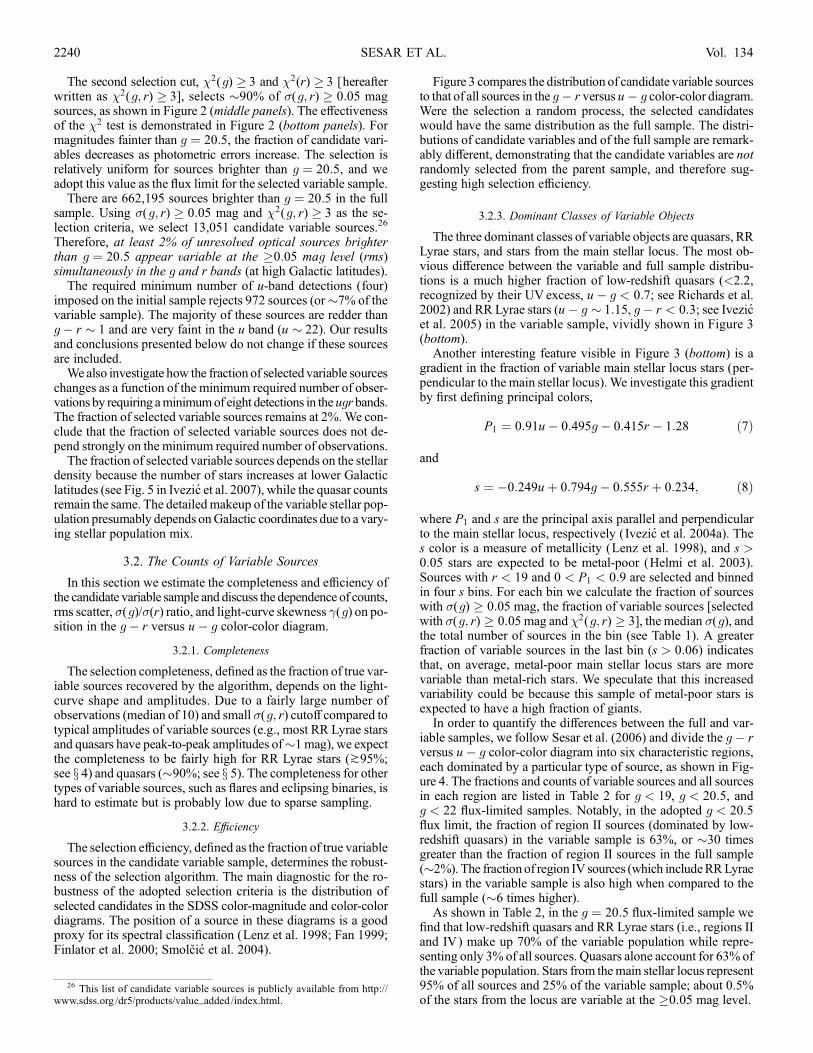
Figure 3 compares the distribution of candidate variable sourcesto that of all sources in the g� r versus u� g color-color diagram.Were the selection a random process, the selected candidateswould have the same distribution as the full sample. The distri-butions of candidate variables and of the full sample are remark-ably different, demonstrating that the candidate variables are notrandomly selected from the parent sample, and therefore sug-gesting high selection efficiency.

3.2.3. Dominant Classes of Variable Objects

The three dominant classes of variable objects are quasars, RRLyrae stars, and stars from the main stellar locus. The most ob-vious difference between the variable and full sample distribu-tions is a much higher fraction of low-redshift quasars (<2.2,recognized by their UV excess, u� g < 0:7; see Richards et al.2002) and RR Lyrae stars (u� g � 1:15, g� r < 0:3; see Ivezicet al. 2005) in the variable sample, vividly shown in Figure 3(bottom).Another interesting feature visible in Figure 3 (bottom) is a

gradient in the fraction of variable main stellar locus stars (per-pendicular to the main stellar locus). We investigate this gradientby first defining principal colors,

P1 ¼ 0:91u� 0:495g� 0:415r � 1:28 ð7Þ

and

s ¼ �0:249uþ 0:794g� 0:555r þ 0:234; ð8Þ

where P1 and s are the principal axis parallel and perpendicularto the main stellar locus, respectively ( Ivezic et al. 2004a). Thes color is a measure of metallicity (Lenz et al. 1998), and s >0:05 stars are expected to be metal-poor (Helmi et al. 2003).Sources with r < 19 and 0 < P1 < 0:9 are selected and binnedin four s bins. For each bin we calculate the fraction of sourceswith �(g) � 0:05 mag, the fraction of variable sources [selectedwith �(g; r) � 0:05mag and �2(g; r) � 3], the median �(g), andthe total number of sources in the bin (see Table 1). A greaterfraction of variable sources in the last bin (s > 0:06) indicatesthat, on average, metal-poor main stellar locus stars are morevariable than metal-rich stars. We speculate that this increasedvariability could be because this sample of metal-poor stars isexpected to have a high fraction of giants.In order to quantify the differences between the full and var-

iable samples, we follow Sesar et al. (2006) and divide the g� rversus u� g color-color diagram into six characteristic regions,each dominated by a particular type of source, as shown in Fig-ure 4. The fractions and counts of variable sources and all sourcesin each region are listed in Table 2 for g < 19, g < 20:5, andg < 22 flux-limited samples. Notably, in the adopted g < 20:5flux limit, the fraction of region II sources (dominated by low-redshift quasars) in the variable sample is 63%, or �30 timesgreater than the fraction of region II sources in the full sample(�2%). The fraction of region IV sources (which includeRRLyraestars) in the variable sample is also high when compared to thefull sample (�6 times higher).As shown in Table 2, in the g ¼ 20:5 flux-limited sample we

find that low-redshift quasars and RR Lyrae stars (i.e., regions IIand IV) make up 70% of the variable population while repre-senting only 3% of all sources. Quasars alone account for 63% ofthe variable population. Stars from themain stellar locus represent95% of all sources and 25% of the variable sample; about 0.5%of the stars from the locus are variable at the �0:05 mag level.

26 This list of candidate variable sources is publicly available from http://www.sdss.org /dr5/products/value_added /index.html.

SESAR ET AL.2240 Vol. 134

3.3. The Properties of Variable Sources

Various light-curve properties, such as shape and amplitude,are expected to be correlated with stellar types. In this section westudy the distribution of the rms scatter in the u and g bands and the�(g)/�(r) ratio as a functionof theu� g andg� r colors.Toempha-size trends, we bin sources and presentmedian values for each bin.

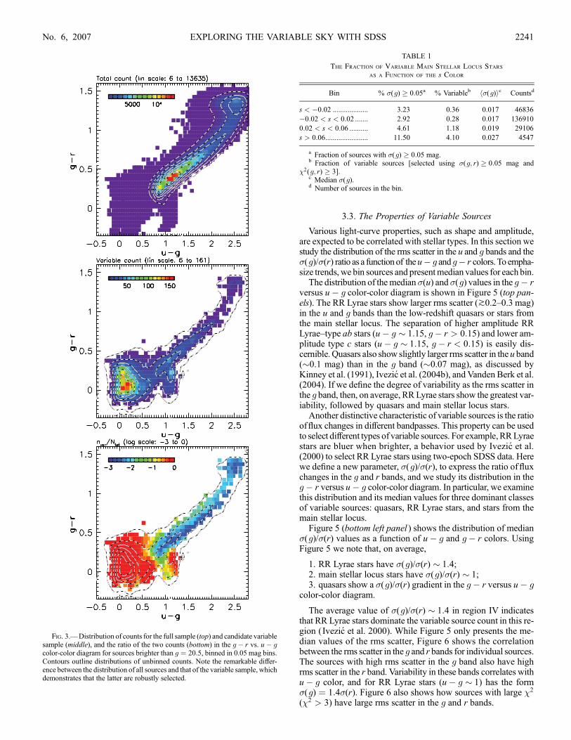
The distribution of themedian�(u) and �(g) values in the g� rversus u� g color-color diagram is shown in Figure 5 (top pan-els). The RR Lyrae stars show larger rms scatter (k0.2Y0.3 mag)in the u and g bands than the low-redshift quasars or stars fromthe main stellar locus. The separation of higher amplitude RRLyraeYtype ab stars (u� g � 1:15, g� r > 0:15) and lower am-plitude type c stars (u� g � 1:15, g� r < 0:15) is easily dis-cernible. Quasars also show slightly larger rms scatter in theu band(�0.1 mag) than in the g band (�0.07 mag), as discussed byKinney et al. (1991), Ivezic et al. (2004b), and Vanden Berk et al.(2004). If we define the degree of variability as the rms scatter inthe g band, then, on average, RRLyrae stars show the greatest var-iability, followed by quasars and main stellar locus stars.

Another distinctive characteristic of variable sources is the ratioofflux changes in different bandpasses. This property can be usedto select different types of variable sources. For example,RRLyraestars are bluer when brighter, a behavior used by Ivezic et al.(2000) to select RR Lyrae stars using two-epoch SDSS data. Herewe define a new parameter, �(g)/�(r), to express the ratio of fluxchanges in the g and r bands, and we study its distribution in theg� r versus u� g color-color diagram. In particular, we examinethis distribution and its median values for three dominant classesof variable sources: quasars, RR Lyrae stars, and stars from themain stellar locus.

Figure 5 (bottom left panel ) shows the distribution of median�(g)/�(r) values as a function of u� g and g� r colors. UsingFigure 5 we note that, on average,

1. RR Lyrae stars have �(g)/�(r) � 1:4;2. main stellar locus stars have �(g)/�(r) � 1;3. quasars show a �(g)/�(r) gradient in the g� r versus u� g

color-color diagram.

The average value of �(g)/�(r) � 1:4 in region IV indicatesthat RR Lyrae stars dominate the variable source count in this re-gion (Ivezic et al. 2000). While Figure 5 only presents the me-dian values of the rms scatter, Figure 6 shows the correlationbetween the rms scatter in the g and r bands for individual sources.The sources with high rms scatter in the g band also have highrms scatter in the r band. Variability in these bands correlates withu� g color, and for RR Lyrae stars (u� g � 1) has the form�(g) ¼ 1:4�(r). Figure 6 also shows how sources with large �2

(�2 > 3) have large rms scatter in the g and r bands.

Fig. 3.—Distribution of counts for the full sample (top) and candidate variablesample (middle), and the ratio of the two counts (bottom) in the g� r vs. u� gcolor-color diagram for sources brighter than g ¼ 20:5, binned in 0.05 mag bins.Contours outline distributions of unbinned counts. Note the remarkable differ-ence between the distribution of all sources and that of the variable sample, whichdemonstrates that the latter are robustly selected.

TABLE 1

The Fraction of Variable Main Stellar Locus Stars

as a Function of the s Color

Bin % �(g) � 0:05a % Variableb h�(g)ic Countsd

s < �0:02 ................... 3.23 0.36 0.017 46836

�0:02 < s < 0:02 ....... 2.92 0.28 0.017 136910

0:02 < s < 0:06 .......... 4.61 1.18 0.019 29106

s > 0:06....................... 11.50 4.10 0.027 4547

a Fraction of sources with �(g) � 0:05 mag.b Fraction of variable sources [selected using �(g; r) � 0:05 mag and

�2(g; r) � 3].c Median �(g).d Number of sources in the bin.

EXPLORING THE VARIABLE SKY WITH SDSS 2241No. 6, 2007

The average ratio of �(g)/�(r) � 1 (i.e., gray flux variations)for stars in the main stellar locus suggests that variability couldbe caused by eclipsing systems. The distribution of �(g) for mainstellar locus stars further strengthens this possibility, as discussedin x 3.4.

The gradient in the �(g)/�(r) ratio observed for low-redshiftquasars in the g� r versus u� g color-color diagram suggeststhat the variability correlation between the g and r bands is morecomplex than in the case of RR Lyrae or main stellar locus stars.Wilhite et al. (2005) show that the photometric color changes forquasars depend on the combined effects of continuum changes,emission-line changes, redshift, and the selection of photometricbandpasses. They note that due to the lack of variability of the

lines, measured photometric color is not always bluer in brighterphases but depends on redshift and the filters used. To verify thedependence of broadband photometric variability on redshift, weplot �(g)/�(r) versus redshift for all spectroscopically confirmedunresolved quasars from Schneider et al. (2005) that are in stripe82, as shown in Figure 7. We confirm that the broadband pho-tometric variability depends on the redshift, and that the �(g)/�(r)gradient in the g� r versus u� g color-color diagram can be ex-plained by the increase in �(g)/�(r) from�1 to�1.6 in the 1.0Y1.6 redshift range. This effect is due to theMg ii emission line (morestable in flux than the continuum) moving through the r-bandfilter over this redshift range. The implied correlation of the u� gand g� r colors with redshift is consistent with the discussion by

Fig. 4.—Distribution of 18,329 candidate variable sources brighter than g ¼ 21 in representative SDSS color-magnitude and color-color diagrams. Candidate variablesare color-coded by their rms scatter in the g band (for 0.05Y0.2, see the legend; for larger than or equal to 0.2, red ). Only sources brighter than g ¼ 20 are plotted in thecolor-color diagrams. Note that RR Lyrae stars [u� g � 1:15, �(g)k0:2 mag; red dots] and low-redshift quasars [u� g � 0:7, �(g)k0:1 mag; green dots] stand out ashighly variable sources. The regions marked in the top right panel are used for quantitative comparison of the overall and variable source distributions (see Table 2).


Richards et al. (2002). The lack of noticeable correlation of �(g)with redshift is due to the combined effects of the dependence of�(g) on the rest-framewavelength and time, which cancel out (fora detailed model, see Ivezic et al. 2004b).

3.4. Skewness as a Proxy for the DominantVariability Mechanism

Light-curve skewness, a measure of the light-curve asymmetry,provides additional information on the type of variability. Neg-atively skewed, asymmetric light curves indicate variable sour-ces that spendmore time fainter than (mmin þ mmax)/2, wheremmin

and mmax are magnitudes at the minimum and maximum. Typeab RR Lyrae stars, for example, have negatively skewed lightcurves (� � �0:5; Wils et al. 2006). Positively skewed, asym-metric light curves indicate variable sources that spend more timebrighter than (mmin þ mmax)/2 (e.g., eclipsing systems). Sourceswith symmetric light curves will have � � 0.

Figure 5 (bottom right panel ) shows the distribution of themedian �(g) as a function of position in the g� r versus u� gcolor-color diagram. On average, quasars and c-type RR Lyraestars (u� g � 1:15, g� r < 0:15) have �(g) � 0, ab-type RRLyrae stars (u� g � 1:15, g� r > 0:15) have negative skew-ness [�(g) � �0:5], and stars in the main stellar locus have pos-itive skewness.

Figure 8 shows the distribution of the light-curve skewness inthe ugi bands for spectroscopically confirmed unresolved quasarsfrom Schneider et al. (2005), which are in stripe 82; candidateRR Lyrae stars (selection details are discussed in x 4); and mainstellar locus stars from our variable sample. Stars in the mainstellar locus show a bimodal �(g) distribution. This distributionsuggests at least two, and perhaps more, different populations ofvariables. Indeed, when spectroscopically confirmedMdwarfs areselected, a third peak appears at �(g) � 2:5, possibly associatedwith flaring M dwarfs (A. Kowalski et al. 2007, in preparation).A bimodality similar to that in the g band is also discernible in ther band, while it is less pronounced in the i band and not detectedin the u and z bands (the r and z data are not shown). The bi-modality in the u and z bands is not detected due to high photo-metric errors in these bands at faint magnitudes. Themeasurementuncertainty decreases the asymmetry of the light curve, and �approaches 0. The less pronounced bimodality in the i bandmightbe due to astrophysical reasons, since the photometric errors in thei band are comparable to g- and r-band photometric errors.

A comparison of the u� g and g� r color distributions for var-iable main stellar locus stars brighter than g ¼ 19 and a subsetwith highly asymmetric light curves [�(g) > 2:5] is shown inFigure 9. The subsetwith asymmetric light curves has an increasedfraction of stars with colors u� g � 2:5 and g� r � 1:4 that cor-respond to M stars. This may indicate that M stars have a higherprobability of being associated with an eclipsing companion thanstars with earlier spectral types. However, the selection effects areprobably important, since a companion is easier to detect (due tothe low luminosity ofMdwarfs).A.Kowalski et al. (2007, in prep-aration) examine these issues using light-curve data on a sample ofspectroscopically confirmedMdwarfs. Finally, quasars have sym-metric light curves (� � 0) and their distribution of skewness doesnot change between bands.

While the value of the skewness for individual sources maystrongly depend on the number of available epochs, the medianbinned values of skewness are not very sensitive to the number ofavailable epochs. We verify this claim by repeating the analysispresented above on a subsample of sources with at least eight de-tections in the ugr bands. A more conservative cut results in asmaller sample, but general trends and results remain the same.

4. THE MILKY WAY HALO STRUCTURE TRACEDBY CANDIDATE RR LYRAE STARS

Studies of substructures in the Galactic halo, such as clumpsand streams, can constrain the formation history of theMilkyWay.Among the best tracers for studying the outer halo are RR Lyraestars, because they are nearly standard candles, are sufficientlybright to be detected at large distances (5Y100 kpc for 14 <r < 20:7), and are sufficiently numerous to trace the halo sub-structure with a high spatial resolution. The General Catalog ofVariable Stars (GCVS; Kholopov et al. 1988) lists27 RR Lyraestars as RR Lyrae type ab (RRab) and type c (RRc) stars. RRabstars have asymmetric light curves, periods from 0.3 to 1.2 days,and amplitudes from V � 0:5 to 2. RRc stars have nearly sym-metric, sometimes sinusoidal, light curves with periods from 0.2to 0.5 days and amplitudes not greater than V � 0:8. In this workwe assumeMV ¼ 0:7 as the absolute V-band magnitude of RRaband RRc stars. A comprehensive review of RR Lyrae stars can befound in Smith (1995).

TABLE 2

The Distribution of Candidate Variable Sources in the g� r versus u� g Diagram

g < 19 g < 20:5 g < 22

Regiona

Nameb % Allc % Var.d Var./Alle Nvar /N

fall % Allc % Var.d Var./Alle Nvar /N

fall % Allc % Var.d Var./Alle Nvar /N

fall

I ...................... White dwarfs 0.14 0.59 4.25 3.50 0.24 0.40 1.69 3.34 0.28 0.45 1.64 4.51

II ..................... Low-redshift QSOs 0.45 30.88 68.83 56.58 1.90 62.90 33.03 65.10 4.07 70.01 17.22 47.30

III.................... dM/WD pairs 0.08 0.53 6.54 5.37 0.83 2.08 2.50 4.92 1.21 3.79 3.13 8.61

IV ................... RR Lyrae stars 1.28 16.81 13.11 10.78 1.33 7.95 5.99 11.81 1.48 6.41 4.33 11.90

V..................... Stellar locus stars 96.27 48.77 0.51 0.42 94.49 25.15 0.27 0.52 91.89 18.33 0.20 0.55

VI ................... High-redshift QSOs 1.78 2.42 1.36 1.12 1.21 1.52 1.26 2.48 1.07 1.01 0.95 2.60

Total count 411667 3384 662195 13051 748067 20553

a These regions are defined in the g� r vs. u� g color-color diagram, with their boundaries shown in Fig. 4.b An approximate description of the dominant source type found in the region.c The fraction of all sources in a magnitude-limited sample found in this color region, with the magnitude limits listed on top.d The number of candidate variables from the region, expressed as a fraction of all variable sources.e The ratio of values listed in the two columns immediately preceding.f The number of candidate variables from the region, expressed as a fraction of all sources in that region.

27 A list of GCVS variability types can be found at http://www.sai.msu.su /groups/cluster/gcvs/gcvs/iii /vartype.txt.


In this section we fine-tune criteria for selecting candidate RRLyrae stars and estimate the selection completeness and efficiency.Using selected candidate RRLyrae stars, we recover a known haloclump associated with the Sgr dwarf tidal stream and find severalnew halo substructures.

4.1. Criteria for Selecting RR Lyrae Stars

Figures 3Y5 show that RR Lyrae stars occupy a well-definedregion (region IV) in the g� r versus u� g color-color diagram,and Figure 6 shows how RR Lyrae stars follow the �(g) ¼1:4�(r) relation. Motivated by these results, we introduce colorand �(g)/�(r) cuts to specifically select candidate RR Lyrae stars

from the variable sample and study their distribution in the rmsscatterYcolorYlight-curve skewness parameter space.RR Lyrae stars have distinctive colors and can be selected

with the following criteria ( Ivezic et al. 2005):

0:98 < u� g < 1:30; ð9Þ

�0:05 < Dug < 0:35; ð10Þ0:06 < Dgr < 0:55; ð11Þ

�0:15 < r � i < 0:22; ð12Þ�0:21 < i� z < 0:25; ð13Þ

Fig. 5.—Distribution of the rms scatter �(u) (top left), rms scatter �(g) (top right), �(g)/�(r) ratio (bottom left), and �(g) (bottom right) for the variable sample in theg� r vs. u� g color-color diagram. Sources are binned in 0.05magwide bins, and themedian values are color-coded. Color ranges are given at the top of each panel, fromblue to red, where green is in the midrange. Values outside the range saturate in blue or red. Contours outline the count distributions on a linear scale in steps of 15%. Theflux limit is g < 20:5, with an additional u < 20:5 limit in the top left panel. Top panels: Note how higher amplitude RRab (u� g � 1:15, g� r > 0:15) and loweramplitude RRc stars (u� g � 1:15, g� r < 0:15) separate in these plots. Bottom left: On average, RR Lyrae stars have �(g)/�(r) � 1:4, main stellar locus stars have�(g)/�(r) � 1, and low-redshift quasars show a gradient of �(g)/�(r) values. Bottom right: On average, quasars and RRc stars have �(g) � 0, RRab stars have negativeskewness, and stars in the main stellar locus have positive skewness.


where

Dug ¼ (u� g)þ 0:67(g� r)� 1:07 ð14Þ

and

Dgr ¼ 0:45(u� g)� (g� r)� 0:12: ð15Þ

We apply these cuts to our sample of candidate variables andselect 846 sources. It is implied by Ivezic et al. (2005) that RRLyrae stars should always staywithin these color boundaries, eventhough their colors change as a function of phase. Their distribu-tion in the g� r versus u� g color-color diagram and rms scatterin the g band are shown in Figure 10 (top left panel ). The dis-tribution of sources in the RR Lyrae region is inhomogeneous.Sources with large rms scatter in the g band (k0.2 mag) are cen-tered around u� g � 1:15 and are separated by g� r � 0:12 intotwo groups. A comparisonwith Figure 3 from Ivezic et al. (2005)suggests that these large rms scatter sources might be RRab(g� r > 0:12) and RRc (g� r < 0:12) stars. Small rms scattersources (P0.1 mag) have a fairly uniform distribution and areslightly bluer, with u� gP 1:1.

The distribution of sources from theRRLyrae region in the�(r)versus �(g) diagram is presented in Figure 10 (top right panel ).The majority of large rms scatter sources follow the �(g) ¼1:4�(r) relation, as expected for RR Lyrae stars. Since RR Lyraestars are bluer when brighter or, equivalently, have greater rmsscatter in the g band than in the r band, we require 1< �(g)/�(r) �2:5 and select 683 candidate RR Lyrae stars.

A comparison of u� g color distributions for candidate RRLyrae stars and of sources with RR Lyrae colors but not tagged asRR Lyrae stars, presented in Figure 10 (bottom left panel ), dem-onstrates the robustness of the RR Lyrae selection. The two dis-tributions are very different (the probability that they are the sameis 10�4, as given by the Kolmogorov-Smirnov test), with the can-didateRRLyrae distribution peaking at u� g � 1:15, as expectedfor RR Lyrae stars.

One property that distinguishes RRab from RRc stars is theshape (or skewness) of their light curves (in addition to light-curveamplitude and period). RRab stars have asymmetric light curves,while RRc light curves are symmetric. In Figure 10 (top left panel )we noted that g� r � 0:12 seemingly separates high rms scattersources into two groups. If g� r � 0:12 is the boundary betweenthe RRab and RRc stars, then the same boundary should show upin the distribution of light-curve skewness as a function of g� rcolor. As shown in Figure 10 (bottom right panel ), this is indeedthe case. On average, sources with g� r < 0:12 have � (g) � 0(symmetric light curves), as do RRc stars, while g� r > 0:12sources have � (g) ��0:5 (asymmetric light curves) typical ofRRab stars.

We show in x 4.2 that candidate RR Lyrae stars with �(g) > 1are contaminated by eclipsing variables. Therefore, to reduce the

Fig. 6.—Distribution of candidate variable sources in the g < 20:5 flux-limited sample. This is shown by linearly spaced contours and by symbols color-codedwith the u� g color for sourceswith�(g) � 0:05 and�(r) � 0:05mag. Thedotted lines show the adopted �(g; r) selection cut. The solid line shows �(g) ¼�(r), while the dashed line shows the �(g) ¼ 1:4�(r) relation representative ofRR Lyrae stars. Note that sources following the �(g) ¼ 1:4�(r) relation tend tohave u� g � 1, as expected for RR Lyrae stars. The gray-scale backgroundshows the fraction of �2(g; r) � 3 that also has �(g) � x and �(r) � y and dem-onstrates that large �2 sources also have large �.

Fig. 7.—Dependence of �(g)/�(r) (top), g� r (middle), and �(g) (bottom) onredshift for a sample of spectroscopically confirmed unresolved quasars fromSchneider et al. (2005). The�(g)/�(r) gradient shown in Fig. 5 (bottom left panel )can be explained by the local maximum of �(g)/�(r) in the 1.0Y1.6 redshift range.


contamination by eclipsing variables, we also require �(g) � 1 andselect 634 sources as our final sample of candidate RRLyrae stars.

4.2. Completeness and Efficiency

The selection completeness, defined as the fraction of re-covered RR Lyrae stars, will depend on the color cuts, the �(g; r)cutoff, and the number of observations. The color cuts (eqs. [9]Y[15]) applied in x 4.1 were chosen to minimize contamination bysources other than RR Lyrae stars while maintaining an almost100% completeness (Ivezic et al. 2005).With the �(g; r) cutoff at0.05 mag (small compared to the �1 mag typical peak-to-peakamplitudes of RR Lyrae stars) and a fairly large number of ob-servations per source (median of 10), we estimate the RR Lyraeselection completeness to bek95% (see the Appendix in Ivezicet al. 2000).To determine the selection efficiency, defined as the fraction of

true RR Lyrae stars in the RR Lyrae candidate sample, we posi-tionally match 683 candidate RR Lyrae stars selected by 1 <�(g)/�(r)� 2:5 to a sample ofRRLyrae sources selected from theSDSS Light-Motion-Curve Catalog (LMCC; D. Bramich et al.2007, in preparation). This catalog covers a slightly smaller regionof the sky (20h42m < � J2000:0 < 03h16m, �1:26� < �J2000:0 <þ1:26�) than that discussed here but includes more densely sam-pled SDSS-II observations that allow the construction of lightcurves. We match 613 candidates, while 70 candidate RR Lyraestars from our sample are not in the LMCC footprint. Followingthe classification based on phased light curves byN. De Lee et al.(2007, in preparation) we find that 71% of 1< �(g)/�(r) � 2:5,�(g) � 1 sources in our candidate RR Lyrae sample are classifiedas RRab and RRc, 28% are classified as variable nonYRR Lyraestars, and only 1% of sources in this sample are classified as spu-rious, nonvariable sources. While we do not know exactly thecompleteness of the N. De Lee et al. (2007, in preparation)samples (efficiency is about 100%, as verified by the visual in-spection of light curves), we speculate that it is likely very high,givenmore densely sampled observations available in the SDSS-IISupernova Survey. The most significant contamination in ourcandidate RR Lyrae sample comes from a population of variablesources bluer than u� g � 1:1 (Fig. 11, dotted line in bottom leftpanel ), possibly Population II � Scuti stars, also known as SXPhoenicis stars (Hoffmeister et al. 1985).The top left and the bottom right panels in Figure 11 show that

RRab- and RRc-dominated regions are separated by g� r �0:12, as already hinted in Figure 10. Also, variable nonYRRLyraesources with �(g) > 1 are classified by N. De Lee et al. (2007, inpreparation) as eclipsing variables, justifying our �(g) � 1 cut.To summarize, using color criteria and criteria based on �(g),

�(r), and �(g), RR Lyrae stars are selected withk95% complete-ness and �70% efficiency.

4.3. The Spatial Distribution of Candidate RR Lyrae Stars

Using the selection criteria from x 4.1we isolate 634 RRLyraecandidates. The magnitude-position diagram for these candidateswithin 2.5

�of the celestial equator is shown in Figure 12.

As discussed by Ivezic et al. (2005), an advantage of the datarepresentation utilized in Figure 12 (magnitudeYright ascensiondiagram) is its simplicity; only ‘‘raw’’ data are shown, withoutany postprocessing. However, the magnitude scale is logarithmic,and thus the spatial extent of structures is heavily distorted. In orderto avoid these shortcomings, we have applied a Bayesianmethodfor estimating continuous spatial density distribution developedby Ivezic et al. (2005, theirAppendixB). The resulting densitymapis shown in Figure 13 (right). The advantage of that representation

Fig. 8.—Light-curve skewness distribution in the ugi bands for spectro-scopically confirmed unresolved quasars (dotted line), candidate RR Lyrae stars(dashed line), and variable main stellar locus stars (solid line, region V; see Fig. 4for the definition). The distribution of the skewness in the r band is similar to theg-band distribution, and the distribution of skewness in the z band is similar to theu-band distribution (therefore, the r and z data are not shown). Stars in the mainstellar locus show bimodality in �(g), suggesting at least two, and perhaps more,different populations of variables. Similar bimodality is also discernible in the rband,while it is less pronounced in the i band and not detected in the u and z bands(due to higher photometric errors). Quasars have symmetric light curves (� � 0),and their distribution of skewness does not change between bands. [See theelectronic edition of the Journal for a color version of this figure.]


is that it better conveys the significance of various local over-densities. For comparison,we also showamap of the northern partof the equatorial strip constructed using two-epoch data discussedby Ivezic et al. (2000).

We detect several new halo substructures at k3 � significance(compared to expected Poissonian fluctuations) and present their

approximate locations and properties in Table 3. In order to as-sess the statistical significance of the clumps seen in Figure 13, wehave performed a detailed analysis using random samples of thesame size as the candidate RR Lyrae sample. The samples wereconstructed using flat distributions in magnitude and right ascen-sion, which approximately correspond to a 1/R3 RRLyrae volume

Fig. 9.—Comparison of the u� g (left) and g� r (right) color distributions for variable main stellar locus stars brighter than g ¼ 19 (dashed lines) and a subset withhighly asymmetric light curves [�(g) > 2:5; solid lines]. The subset with highly asymmetric light curves has an increased fraction of stars with colors u� g � 2:5 andg� r � 1:5, characteristic of M stars. [See the electronic edition of the Journal for a color version of this figure.]

Fig. 10.—Top left: Distribution of 846 candidate variable sources from the RR Lyrae region (dashed lines; see Fig. 3 in Ivezic et al. 2005) in the g� r vs. u� g color-color diagram. The symbols mark the time-averaged values and are color-coded by �(g) (0.05Y0.2; blue to red ). The dotted line shows the boundary between the RRab- andRRc-dominated regions. Top right: Sources from the top left panel divided into three groups according to their �(g)/�(r) values: candidate RR Lyrae stars with1 < �(g)/�(r) � 2:5 (large dots), sources with �(g)/�(r) � 1 (triangles), and sources with �(g)/�(r) > 2:5 (squares). Small dots show sources with RR Lyrae colorsthat fail the variability criteria. The dashed lines show the �(g) ¼ �(r) and �(g) ¼ 2:5�(r) relations, while the dotted line shows the �(g) ¼ 1:4�(r) relation. Bottom left:Comparison of the u� g color distributions for candidate RR Lyrae stars (solid line) and sources with RR Lyrae colors but not tagged as RR Lyrae stars (dashed line).Bottom right: Dependence of �(g) on the g� r color for candidate RR Lyrae stars. The boundary g� r ¼ 0:12 (dotted line) separates candidate RR Lyrae stars into thosewith asymmetric [�(g) ��0:5] and symmetric [�(g) � 0] light curves, corresponding to RRab and RRc stars, respectively. The condition �(g) � 1 (dashed line) is usedto reduce the contamination of the RR Lyrae sample by eclipsing variables.


density distribution, whereR is the distance from theGalactic cen-ter. We find that the contamination by nonYRR Lyrae stars is notan issue because this effect tends to minimize the structure, ratherthan enhance it. The random samples often have clumplike fea-tures due to Poisson fluctuations. By comparing the histograms ofdensity distributions for random samples and the observed can-didateRRLyrae sample, we conclude that clumps I andK are con-sistent with random fluctuations, and one or two of clumps D, F,

H, and L may also be caused by such fluctuations. The remainingseven clumps (A, B, C, E, G, J, and M) are inconsistent with ran-dom fluctuations and likely represent real halo substructure. Starsassociated with these clumps account for about 50% of the sam-ple. This estimate for the fraction of halo stars that are associatedwith substructure is in good agreement with estimates based onmain-sequence stars in the inner halo (out to about 30 kpc) by Juricet al. (2007) and Bell et al. (2007).Themost distant clump (M) is 106 kpc from theGalactic center.

The strongest clump in the left wedge belongs to the Sgr dwarftidal stream, as does clumpC in the rightwedge (Ivezic et al. 2003).Similarly to the behavior ofmain-sequence stars discussed byBellet al. (2007), the apparent ‘‘clumpiness’’ of the candidate RRLyraedistribution increaseswith increasing radius, as predicted byCDMsimulations (Bullock et al. 2001). A detailed comparison of theirmodels with the data presented here will be discussed elsewhere(B. Sesar et al. 2007, in preparation).

5. ARE ALL QUASARS VARIABLE?

The optical continuum variability of quasars has been recog-nized since their first optical identification (Matthews & Sandage1963), and it has been proposed and utilized as an efficientmethodfor their discovery (van den Bergh et al. 1973; Hawkins 1983;Koo et al. 1986; Hawkins & Veron 1995; Rengstorf et al. 2004).The observed characteristics of the variability of quasars arefrequently used to constrain the origin of their emission (e.g.,Kawaguchi et al. 1998 and references therein;Martini&Schneider

Fig. 11.—Distribution of candidate RR Lyrae stars selected with 1 < �(g)/�(r) � 2:5 and classified by N. De Lee et al. (2007, in preparation) shown in diagrams similarto Fig. 10. Symbols show RRab stars (red dots), RRc stars (blue dots), variable nonYRR Lyrae stars (green dots), and nonvariable sources (open squares; only four sources).A comparison of the u� g color distribution for RRab (solid line), RRc (dashed line), and variable nonYRR Lyrae stars (dotted line) is shown in the bottom left panel.

Fig. 12.—Magnitude-position distribution of 634 stripe 82 RR Lyrae candi-dateswithin�55� < R:A: < 60� and jdecl:j � 1:27�. Approximate distance (shownon the right y-axis) is calculated assuming Mr ¼ 0:7 mag for RR Lyrae stars.Dashed lines show where sample completeness decreases from approximately99% to 60% due to the�2 cut (see Fig. 2, bottom right panel ). Closed curves areremapped ellipses and circles from Fig. 13 that mark halo substructure. [See theelectronic edition of the Journal for a color version of this figure.]


2003; Pereyra et al. 2006). Recently, significant progress in thedescription of quasar variability has been made by employing theSDSS data (de Vries et al. 2003, 2005; Ivezic et al. 2004b; VandenBerk et al. 2004; Sesar et al. 2006). Here we expand these studiesby quantifying the efficiency of quasar discovery using variability.

A preliminary comparison of color- and variability-basedmeth-ods for selecting quasars using SDSSdatawas presented by Ivezicet al. (2004c). They found that 47%of spectroscopically confirmedunresolved quasars with UVexcess have a g-bandmagnitude dif-ference between two observations obtained 2 yr apart larger than0.15 mag. We can improve on their analysis because now thereare significantly more observations obtained over a longer timeperiod. Since quasars vary erratically and the rms scatter of theirvariability (the so-called structure function) increases with time(e.g., VandenBerk et al. 2004 and references therein), the variabil-ity selection completeness is expected to be higher than �50%,obtained by Ivezic et al. (2004c).

First, although the adopted variability selection criteria dis-cussed above are fairly conservative, we find that at least 63% oflow-redshift quasars are variable at the�0:05 mag level (simul-taneously in the g and r bands over observer’s timescales of sev-eral years) in the g < 20:5 flux-limited sample. Second, even thisestimate is only a lower limit; given the spectroscopic confirma-tion for a large flux-limited sample of quasars, it is possible to relaxthe adopted variability selection cutoff without prohibitive contam-ination by nonvariable sources.

There are 2492 unresolved quasars in the catalog of spectro-scopically confirmed SDSS quasars (Schneider et al. 2005) fromstripe 82. The fraction of these objects that varymore than � in theg and r bands, as a function of �, is shown in Figure 14. We alsoshow the analogous fraction for stars from the stellar locus. About93% of quasars vary with � > 0:03 mag. For a small fraction ofthese objects themeasured rms scatter is due to photometric noise,and the stellar data limit this fraction to at most 3%. Conserva-tively assuming that none of these 3% of stars are intrinsically

25

50

75

100 kpc

A

B

C

D

E

F

G

H

I

J

K

L

M

Fig. 13.—Left: Spatial distribution of candidate RRLyrae stars discovered by SDSS along the celestial equator. Distance is calculated assuming eq. (3) from Ivezic et al.(2005) andMV ¼ 0:7 mag as the absolute magnitude of RR Lyrae stars in the V band. The right wedge corresponds to candidate RR Lyrae stars selected in this work (634candidates, shown in Fig. 12), and the left wedge is based on the sample from Ivezic et al. (2000; 296 candidates).Right: Number density distribution of candidate RRLyraestars shown in the left panel, computed using an adaptive Bayesian density estimator developed by Ivezic et al. (2005). The color scheme represents the number densitymultiplied by the cube of the galactocentric radius and displayed on a logarithmic scale with a dynamic range of 300 (light blue to red ). Green corresponds to the meandensity; both wedges with the data would have this color if the halo number density distribution followed a perfectly smooth r�3 power law. Purple marks the regions withno data. The yellow/orange regions are formally about 3 � significant overdensities, and red regions have an even higher significance (using only the count variance). Acomparison of this map with those generated using random samples of the same size suggests that clumps I and K are consistent with random fluctuations; one or two ofclumps D, F, H, and L may also be caused by such fluctuations; and it is highly likely that the remaining seven clumps (A, B, C, E, G, J, and M) represent real halosubstructure (they account for about 50% of the sample in the right wedge). The strongest clump in the left wedge belongs to the Sgr dwarf tidal stream, as does clump C inthe right wedge (Ivezic et al. 2003). An approximate location and properties of labeled overdensities are listed in Table 3. The Ivezic et al. (2000) sample is based on onlytwo epochs and thus has a much lower completeness (�56%), resulting in a lower density contrast.

TABLE 3

Approximate Locations and Properties of Detected Overdensities

Labela N b hR.A.ic hdid hrie hu� gif hg� rig

A........................... 84 330.95 21 17.02 1.14 0.18

B........................... 144 309.47 22 16.76 1.12 0.16

C........................... 54 33.69 25 17.61 1.13 0.20

D........................... 8 347.91 29 18.02 1.14 0.23

E ........................... 11 314.06 43 18.84 1.09 0.20

F ........................... 11 330.26 48 19.16 1.07 0.20

G........................... 10 354.81 55 19.46 1.10 0.22

H........................... 7 43.57 57 19.32 1.05 0.04

I ............................ 4 311.34 72 19.98 1.08 0.11

J ............................ 26 353.58 81 20.21 1.11 0.20

K........................... 8 28.39 84 20.35 1.10 0.20

L ........................... 3 339.01 92 20.45 1.06 0.16

M.......................... 5 39.45 102 20.73 1.07 0.11

a The overdensity’s label from Fig. 13.b Number of candidate RR Lyrae stars in the overdensity.c Median right ascension.d Median heliocentric distance (in kpc), computed using eq. (3) from Ivezic et al.

(2005) andMV ¼ 0:7mag as the absolutemagnitude ofRRLyrae stars in theVband.e Median r-band magnitude.f Median u� g color.g Median g� r color.


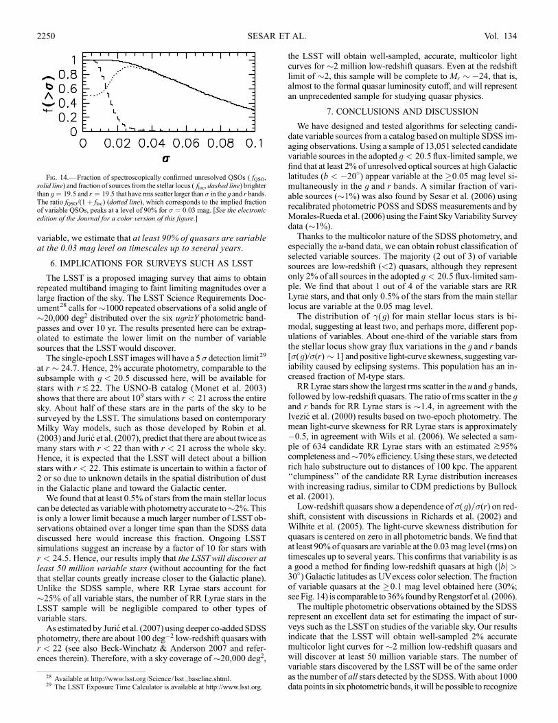
variable, we estimate that at least 90% of quasars are variableat the 0.03 mag level on timescales up to several years.

6. IMPLICATIONS FOR SURVEYS SUCH AS LSST

The LSST is a proposed imaging survey that aims to obtainrepeated multiband imaging to faint limiting magnitudes over alarge fraction of the sky. The LSST Science Requirements Doc-ument28 calls for�1000 repeated observations of a solid angle of�20,000 deg2 distributed over the six ugrizY photometric band-passes and over 10 yr. The results presented here can be extrap-olated to estimate the lower limit on the number of variablesources that the LSST would discover.

The single-epochLSST imageswill have a 5� detection limit29

at r � 24:7. Hence, 2% accurate photometry, comparable to thesubsample with g < 20:5 discussed here, will be available forstars with rP 22. The USNO-B catalog (Monet et al. 2003)shows that there are about 109 stars with r < 21 across the entiresky. About half of these stars are in the parts of the sky to besurveyed by the LSST. The simulations based on contemporaryMilky Way models, such as those developed by Robin et al.(2003) and Juric et al. (2007), predict that there are about twice asmany stars with r < 22 than with r < 21 across the whole sky.Hence, it is expected that the LSST will detect about a billionstars with r < 22. This estimate is uncertain to within a factor of2 or so due to unknown details in the spatial distribution of dustin the Galactic plane and toward the Galactic center.

We found that at least 0.5% of stars from the main stellar locuscan be detected as variablewith photometry accurate to�2%.Thisis only a lower limit because a much larger number of LSST ob-servations obtained over a longer time span than the SDSS datadiscussed here would increase this fraction. Ongoing LSSTsimulations suggest an increase by a factor of 10 for stars withr < 24:5. Hence, our results imply that the LSSTwill discover atleast 50 million variable stars (without accounting for the factthat stellar counts greatly increase closer to the Galactic plane).Unlike the SDSS sample, where RR Lyrae stars account for�25% of all variable stars, the number of RR Lyrae stars in theLSST sample will be negligible compared to other types ofvariable stars.

As estimated by Juric et al. (2007) using deeper co-added SDSSphotometry, there are about 100 deg�2 low-redshift quasars withr < 22 (see also Beck-Winchatz & Anderson 2007 and refer-ences therein). Therefore, with a sky coverage of�20,000 deg2,

the LSST will obtain well-sampled, accurate, multicolor lightcurves for �2 million low-redshift quasars. Even at the redshiftlimit of �2, this sample will be complete to Mr ��24, that is,almost to the formal quasar luminosity cutoff, and will representan unprecedented sample for studying quasar physics.

7. CONCLUSIONS AND DISCUSSION

We have designed and tested algorithms for selecting candi-date variable sources from a catalog based onmultiple SDSS im-aging observations. Using a sample of 13,051 selected candidatevariable sources in the adopted g < 20:5 flux-limited sample, wefind that at least 2% of unresolved optical sources at high Galacticlatitudes (b < �20�) appear variable at the �0:05 mag level si-multaneously in the g and r bands. A similar fraction of vari-able sources (�1%) was also found by Sesar et al. (2006) usingrecalibrated photometric POSS and SDSS measurements and byMorales-Rueda et al. (2006) using the Faint SkyVariability Surveydata (�1%).Thanks to the multicolor nature of the SDSS photometry, and

especially the u-band data, we can obtain robust classification ofselected variable sources. The majority (2 out of 3) of variablesources are low-redshift (<2) quasars, although they representonly 2% of all sources in the adopted g < 20:5 flux-limited sam-ple. We find that about 1 out of 4 of the variable stars are RRLyrae stars, and that only 0.5% of the stars from the main stellarlocus are variable at the 0.05 mag level.The distribution of �(g) for main stellar locus stars is bi-

modal, suggesting at least two, and perhaps more, different pop-ulations of variables. About one-third of the variable stars fromthe stellar locus show gray flux variations in the g and r bands[�(g)/�(r) � 1] and positive light-curve skewness, suggesting var-iability caused by eclipsing systems. This population has an in-creased fraction of M-type stars.RRLyrae stars show the largest rms scatter in the u and g bands,

followed by low-redshift quasars. The ratio of rms scatter in the gand r bands for RR Lyrae stars is �1.4, in agreement with theIvezic et al. (2000) results based on two-epoch photometry. Themean light-curve skewness for RR Lyrae stars is approximately�0.5, in agreement with Wils et al. (2006). We selected a sam-ple of 634 candidate RR Lyrae stars with an estimated k95%completeness and�70%efficiency.Using these stars, we detectedrich halo substructure out to distances of 100 kpc. The apparent‘‘clumpiness’’ of the candidate RR Lyrae distribution increaseswith increasing radius, similar to CDM predictions by Bullocket al. (2001).Low-redshift quasars show a dependence of �(g)=�(r) on red-

shift, consistent with discussions in Richards et al. (2002) andWilhite et al. (2005). The light-curve skewness distribution forquasars is centered on zero in all photometric bands.We find thatat least 90% of quasars are variable at the 0.03mag level (rms) ontimescales up to several years. This confirms that variability is asa good a method for finding low-redshift quasars at high (jbj >30�) Galactic latitudes as UVexcess color selection. The fractionof variable quasars at the �0:1 mag level obtained here (30%;see Fig. 14) is comparable to 36% foundbyRengstorf et al. (2006).The multiple photometric observations obtained by the SDSS

represent an excellent data set for estimating the impact of sur-veys such as the LSSTon studies of the variable sky. Our resultsindicate that the LSST will obtain well-sampled 2% accuratemulticolor light curves for �2 million low-redshift quasars andwill discover at least 50 million variable stars. The number ofvariable stars discovered by the LSST will be of the same orderas the number of all stars detected by the SDSS.With about 1000data points in six photometric bands, it will be possible to recognize

Fig. 14.—Fraction of spectroscopically confirmed unresolved QSOs ( fQSO,solid line) and fraction of sources from the stellar locus ( floc, dashed line) brighterthan g ¼ 19:5 and r ¼ 19:5 that have rms scatter larger than � in the g and r bands.The ratio fQSO/(1þ floc) (dotted line), which corresponds to the implied fractionof variable QSOs, peaks at a level of 90% for � ¼ 0:03 mag. [See the electronicedition of the Journal for a color version of this figure.]

28 Available at http://www.lsst.org /Science/ lsst_baseline.shtml.29 The LSST Exposure Time Calculator is available at http://www.lsst.org.


and classify variable objects using light-curve moments of higherorder than the skewness discussed here, including light-curve fold-ing for periodic variables.

This work was supported by an NSF-sponsored research sti-pend (NVO 8601-06862) obtained fromNVO through The JohnsHopkins University.We also acknowledge support by NSF grantAST 05-51161 to the LSST for design and development activity.

Funding for the SDSS and SDSS-II has been provided by theAlfred P. Sloan Foundation, the Participating Institutions, theNational Science Foundation, the US Department of Energy,the National Aeronautics and Space Administration, the JapaneseMonbukagakusho, the Max Planck Society, and the Higher Ed-ucation Funding Council for England. The SDSS Web site ishttp://www.sdss.org.

The SDSS is managed by the Astrophysical Research Con-sortium for the Participating Institutions. The ParticipatingInstitutions are the American Museum of Natural History, theAstrophysical Institute Potsdam, the University of Basel, theUniversity of Cambridge, Case Western Reserve University,the University of Chicago, Drexel University, Fermilab, the Insti-tute for Advanced Study, the Japan Participation Group, JohnsHopkins University, the Joint Institute for Nuclear Astrophysics,the Kavli Institute for Particle Astrophysics and Cosmology,the Korean Scientist Group, the Chinese Academy of Sciences,Los Alamos National Laboratory, the Max Planck Institute forAstronomy, the Max Planck Institute for Astrophysics), NewMexico State University, Ohio State University, the Universityof Pittsburgh, the University of Portsmouth, Princeton Univer-sity, the United States Naval Observatory, and the University ofWashington.

REFERENCES

Adelman-McCarthy, J. K., et al. 2007, ApJS, 172, in pressAkerlof, C., et al. 2000, AJ, 119, 1901Alcock, C., et al. 2001, ApJS, 136, 439Becker, A. C., et al. 2004, ApJ, 611, 418Beck-Winchatz, B., & Anderson, S. F. 2007, MNRAS, 374, 1506Bell, E. F, et al. 2007, ApJ, submitted (arXiv:0706.0004)Bullock, J. S., Kravtsov, A. V., & Weinberg, D. H. 2001, ApJ, 548, 33de Vries, W. H., Becker, R. H., & White, R. L. 2003, AJ, 126, 1217de Vries, W. H., Becker, R. H., White, R. L., & Loomis, C. 2005, AJ, 129, 615Fan, X. 1999, AJ, 117, 2528Finlator, K., et al. 2000, AJ, 120, 2615Fukugita, M., Ichikawa, T., Gunn, J. E., Doi, M., Shimasaku, K., & Schneider,D. P. 1996, AJ, 111, 1748

Groot, P. J., et al. 2003, MNRAS, 339, 427Gunn, J. E., et al. 1998, AJ, 116, 3040———. 2006, AJ, 131, 2332Hawkins, M. R. S. 1983, MNRAS, 202, 571Hawkins, M. R. S., & Veron, P. 1995, MNRAS, 275, 1102Hawley, S. L., et al. 2002, AJ, 123, 3409Helmi, A., et al. 2003, ApJ, 586, 195Hoffmeister, C., Richter, G., & Wenzel, W. 1985, Variable Stars (New York:Springer)

Hogg, D. W., Finkbeiner, D. P., Schlegel, D. J., & Gunn, J. E. 2001, AJ, 122,2129

Ivezic, Z., Vivas, A. K., Lupton, R. H., & Zinn, R. 2005, AJ, 129, 1096Ivezic, Z., et al. 2000, AJ, 120, 963———. 2003, Mem. Soc. Astron. Italiana, 74, 978———. 2004a, Astron. Nachr., 325, 583———. 2004b, in IAU Symp. 222, The Interplay among Black Holes, Stars,and ISM in Galactic Nuclei, ed. T. S. Bergmann, L. C. Ho, & H. R. Schmitt(Cambridge: Cambridge Univ. Press), 525

———. 2004c, in ASP Conf. Ser. 311, AGN Physics with the Sloan DigitalSky Survey, ed. G. T. Richards & P. B. Hall (San Francisco: ASP), 437

———. 2007, AJ, 134, 973Juric, M., et al. 2007, AJ, submitted (astro-ph /0510520)Kaiser, N., et al. 2002, Proc. SPIE, 4836, 154Kawaguchi, T., Mineshige, S., Umemura, M., & Turner, E. L. 1998, ApJ, 504,671

Kholopov, P. N., et al. 1988, General Catalog of Variable Stars (4th ed.;Moscow: Nauka)

Kinney, A. L., Bohlin, R. C., Blades, J. C., & York, D. G. 1991, ApJS, 75, 645Koo, D. C., Kron, R. G., & Cudworth, K. M. 1986, PASP, 98, 285Lenz, D. D., Newberg, J., Rosner, R., Richards, G. T., & Stoughton, C. 1998,ApJS, 119, 121

Lupton, R. H., Ivezic, Z., Gunn, J. E., Knapp, G. R., Strauss, M. A., & Yasuda,N. 2002, Proc. SPIE, 4836, 350

Martini, P., & Schneider, D. P. 2003, ApJ, 597, L109Matthews, T. A., & Sandage, A. R. 1963, ApJ, 138, 30Monet, D. G., et al. 2003, AJ, 125, 984Morales-Rueda, L., Groot, P. J., Augusteijn, T., Nelemans, G., Vreeswijk, P. M.,& van den Besselaar, E. J. M. 2006, MNRAS, 371, 1681

National Research Council. 2001, Astronomy and Astrophysics in the NewMillennium (Washington: Natl. Acad. Press)

Pereyra, N. A., Vanden Berk, D. E., & Turnshek, D. A. 2006, ApJ, 642, 87Pier, J. R., Munn, J. A., Hindsley, R. B., Hennesy, G. S., Kent, S. M., Lupton,R. H., & Ivezic, Z. 2003, AJ, 125, 1559

Pojmanski, G. 2002, Acta Astron., 52, 397Rengstorf, A. W., Brunner, R. J., & Wilhite, B. C. 2006, AJ, 131, 1923Rengstorf, A. W., et al. 2004, ApJ, 606, 741Richards, G. T., et al. 2002, AJ, 123, 2945Robin, A. C., Reyle, C., Derriere, S., & Picaud, S. 2003, A&A, 409, 523Schlegel, D., Finkbeiner, D. P., & Davis, M. 1998, ApJ, 500, 525Schneider, D. P., et al. 2005, AJ, 130, 367Scranton, R., et al. 2002, ApJ, 579, 48Sesar, B., et al. 2006, AJ, 131, 2801Sirko, E., et al. 2004, AJ, 127, 899Smith, H. A. 1995, RR Lyrae Stars (Cambridge: Cambridge Univ. Press)Smith, J. A., et al. 2002, AJ, 123, 2121Smolcic, V., et al. 2004, ApJ, 615, L141Stoughton, C., et al. 2002, AJ, 123, 485Strateva, I., et al. 2001, AJ, 122, 1861Trevese, D., Kron, R. G., & Bunone, A. 2001, ApJ, 551, 103Tucker, D., et al. 2006, Astron. Nachr., 327, 821Tyson, J. A. 2002, Proc. SPIE, 4836, 10Udalski, A., Zebrun, K., Szymanski, M., Kubiak, M., Soszynski, I., Szewczyk,O., Wyrzykowski, L., & Pietrzynski, G. 2002, Acta Astron., 52, 115

van den Bergh, S., Herbst, E., & Pritchet, C. 1973, AJ, 78, 375Vanden Berk, D. E., et al. 2004, ApJ, 601, 692Vivas, A. K., et al. 2004, AJ, 127, 1158Walker, A. R. 2003, Mem. Soc. Astron. Italiana, 74, 999Wilhite, B. C., Vanden Berk, D. E., Kron, R. G., Schneider, D. P., Pereyra, N.,Brunner, R. J., Richards, G. T., & Brinkmann, J. V. 2005, ApJ, 633, 638

Wils, P., Lloyd, C., & Bernhard, K. 2006, MNRAS, 368, 1757Wozniak, P. R., Udalski, A., Szymanski, M., Kubiak, M., Pietrzynski, G.,Soszynski, I., & Zebrun, K. 2002, Acta Astron., 52, 129

Wozniak, P. R., et al. 2004, AJ, 127, 2436Yanny, B., et al. 2000, ApJ, 540, 825York, D. G., et al. 2000, AJ, 120, 1579Zebrun, K., et al. 2001, Acta Astron., 51, 317


exploring the variable sky with the sloan digital sky survey

Documents