Exploring the use of dynamic linear panel data modelsfor evaluating energy/economy/environment models —an application for the transportation sector

A. Schäfer & P. Kyle & R. Pietzcker

# The Author(s) 2014. This article is published with open access at Springerlink.com

Abstract This paper uses the RoSE transportation sector scenarios of the GCAM andREMIND energy-economy-models for the U.S. region to derive and compare these models’intrinsic elasticities with those resulting from historical trends, estimates from the literature,and across each other. To estimate the model-intrinsic elasticities, we explore the use ofdynamic linear panel data models. On the basis of 26 scenarios (panels) between 2010 and2050, our analysis suggests that nearly all model-intrinsic elasticities with respect to finalenergy use are roughly comparable to each other, to those observed historically, and to thosefrom other studies. The key difference is these models’ comparatively low intrinsic incomeelasticity of final energy use. This and other minor differences are interpreted through keyassumptions underlying both energy-economy-models.

1 Introduction

As economies develop and the value added shifts from agriculture to industry to services,energy use by and CO2 emissions from transportation continue to increase in both absolute andrelative terms (see, e.g., Schäfer et al. 2009). Because of this rising importance, it is imperativeto understand why long-term projections of this sector’s energy use and CO2 emissions differacross models, and how these projections’ underlying key characteristics compare to thoseobserved historically.

DOI 10.1007/s10584-014-1293-y

This article is part of a Special Issue on “The Impact of Economic Growth and Fossil Fuel Availability onClimate Protection” with Guest Editors Elmar Kriegler, Ottmar Edenhofer, Ioanna Mouratiadou, Gunnar Luderer,and Jae Edmonds.

A. Schäfer (*)UCL Energy Institute, University College London, London, UKe-mail: a.schafer@ucl.ac.uk

A. SchäferPrecourt Energy Efficiency Center, Stanford University, Stanford, USA

P. KylePacific Northwest Laboratory, Joint Global Change Research Institute, College Park, USA

R. PietzckerPotsdam Institute for Climate Impact Research, Potsdam, Germany

Received: 5 March 2013 /Accepted: 12 November 2014 /Published online: 25 November 2014

Climatic Change (2016) 136:141–154

The effort to compare and improve energy-economy-models has a long history. StanfordUniversity’s Energy Modeling Forum, which pursues these and related goals, already started in1976 (EMF 1977). The usual approach has been to run the evaluated models under consistentassumptions of key determinants of energy use and associated CO2 emissions and then tosystematically compare the outputs. Doing so, differences in model outputs are traced back to thoseof individual components, thus identifying key uncertainties with respect to model structure andchosen parameters. The RoSE project, to which this paper contributes, is one of many examples.

In this paper, we pursue an alternative approach by estimating and comparing the model-intrinsic elasticities across each other and with those of the historical trend. Varying the inputsinto the energy-economy-models causes a responsiveness in the outputs. A sufficiently largenumber of scenarios with different model input assumptions (and therefore outputs) thenconstitutes a set of panels, which can be used to estimate the key aggregate characteristicsof the underlying model. The obtained intrinsic elasticities account for the underlying modelstructure, embedded functional forms, assumptions about the substitutability of energy ser-vices, along technologies and their characteristics. This approach’s advantage is that theestimated elasticities can be readily compared to each other, to those from the literature, andto those underlying the historical development, irrespective of the type of energy-economy-model examined. In addition, this approach does not depend on the use of identical assump-tions of key determinants of energy use and associated CO2 emissions that serve as inputs intothe models that are being compared. While there is a growing body of literature on validatingenergy-economy-models (Schwanitz 2013; Beckman et al. 2011; Wilson et al. 2013), we knowof no research that would have taken our approach and compared model-intrinsic elasticities toeach other and historic values.

We apply this approach to the transportation sector. Among the energy-economy-modelsused in the RoSE project, only GCAM and REMIND incorporate a transportation sector that isendogenously embedded within the energy economy. Although both models fall into the“hybrid energy models” category, they have important structural differences, which are likelyto lead to different model outputs, despite consistent input assumptions with respect toeconomic growth, population, and the amount of fossil fuel resources.

This paper continues with describing the long-term historical and projected future trends inthe U.S. transportation sector in terms of energy use, and its key determinants. Beforespecifying econometric models that allow estimating the historical elasticities and thoseintrinsic to the two energy-economy-models, the properties of the time series data need tobe examined with respect to integrated processes that would render standard estimationtechniques invalid. Thereafter we present the statistical models used to estimate the keyelasticities that describe past trends in U.S. transport sector energy use and the projected levelsfrom the GCAM and REMIND models. Then we interpret the results using the key features ofthe two energy models before summarizing and concluding this study’s findings.

2 Key characteristics of U.S. transportation energy use

Figures 1a–d illustrate the historical and projected future levels of transport sector related finalenergy use, the weighted average consumer fuel prices, along key model inputs, i.e., GDP perperson and population.

As depicted in Fig. 1a, between 1920 and 2010, final energy use in U.S. transportationmultiplied by a factor of around 6 (Schäfer 2013). The model-projected future levels oftransport sector final energy use differ widely, depending on the scenario. However, commonto both model outputs is a strongly reduced future growth, an eventual leveling off and decline

Climatic Change (2016) 136:141–154142

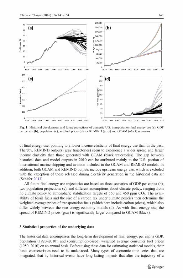
of final energy use, pointing to a lower income elasticity of final energy use than in the past.Thereby, REMIND outputs (gray trajectories) seem to experience a wider spread and largerincome elasticity than those generated with GCAM (black trajectories). The gap betweenhistorical data and model outputs in 2010 can be attributed mainly to the U.S. portion ofinternational marine shipping and aviation included in the GCAM and REMIND models. Inaddition, both GCAM and REMIND outputs include upstream energy use, which is excludedwith the exception of those released during electricity generation in the historical data set(Schäfer 2013).

All future final energy use trajectories are based on three scenarios of GDP per capita (b),two population projections (c), and different assumptions about climate policy, ranging fromno climate policy to atmospheric stabilization targets of 550 and 450 ppm CO2. The avail-ability of fossil fuels and the size of a carbon tax under climate policies then determine theweighted average prices of transportation fuels (which here include carbon prices), which alsodiffer widely between the two energy-economy-models (d). As with final energy use, thespread of REMIND prices (gray) is significantly larger compared to GCAM (black).

3 Statistical properties of the underlying data

The historical data encompasses the long-term development of final energy, per capita GDP,population (1920–2010), and (consumption-based) weighted average consumer fuel prices(1950–2010) on an annual basis. Before using these data for estimating statistical models, theirbasic characteristics need to be understood. Many types of economic time series data areintegrated, that is, historical events have long-lasting impacts that alter the trajectory of a

Fig. 1 Historical development and future projections of domestic U.S. transportation final energy use (a), GDPper person (b), population (c), and fuel prices (d) for REMIND (gray) and GCAM (black) scenarios

Climatic Change (2016) 136:141–154 143

variable far into the future. Such non-stationary characteristics would make the coefficient andvariance estimates meaningless. Therefore we conduct unit root or order of integration tests forthe variables individually.

Figure 2 depicts the development of the four variables in terms of the natural logarithm ofthe levels (left column) and first differences (right column) for 61 years starting in 1950. Thelevels of the historical series in the left column in Fig. 2 appear non-stationary, i.e., have a unitroot. In contrast, the first-differenced variables in the right column, with the exception ofperhaps population, seem to be stationary. The first differences of the logarithms of finalenergy use appear to be trend stationary until the early 1970s and then stationary. Given thedevelopment of the levels of the variables of interest and that of the first differences, we addeda trend term to the unit root tests for the variable in levels and a drift term when testing the firstdifferences for unit roots.

The results of the unit root tests are shown in Table 1. The Augmented Dickey-Fuller(ADF) statistic of the underlying test of the historical time series data suggests clear evidenceof a unit root in levels of all variables except the logarithm of population. (The null hypothesisis that the data series are non-stationary). However, first-differencing the data leads tostationary properties at a confidence level of at least 95 % (** in Table 1) for all time series.Since all the series have a unit root and the order of integration is one, there may exist astatistical relation of the series in their levels that is stationary, suggesting cointegration.

As a basis for estimating the panel data models, we selected 26 scenarios that weresimulated by both energy-economy-models. These scenarios can be classified in three familieswith internally consistent assumptions (Groups 1–3) and a fourth family with two remainingscenarios (Group 4). For a detailed description of the scenarios, see Kriegler et al. (this issue).

& Group 1: 8 baseline scenarios with different combinations of growth in income andpopulation and the availability of fossil fuel resources (of which only the assumptionsabout the availability of oil are critical for the transportation sector)

& Group 2: 8 mitigation scenarios eventually leading to an atmospheric concentration ofgreenhouse gas emissions of 550 ppm of CO2 equivalent

& Group 3: 8 mitigation scenarios eventually leading to an atmospheric concentration ofgreenhouse gas emissions of 450 ppm of CO2 equivalent

& Group 4: 2 additional scenarios describing a moderate policy case and a scenario reaching450 ppm CO2 equivalent by 2100 despite moderate policies until 2020

We also tested the GCAM and REMIND model outputs between 2010 and 2050,the period for which we obtained panel data with 5-year time steps, for unit roots.The employed ADF test rejected the null hypothesis that all panels would contain aunit root. As will be shown in Table 3 below, the elasticity of the lagged dependentvariable is around 0.5 and thus far from unity, also eliminating any concern about thepossible existence of unit roots. For brevity, we therefore do not report here the ADFtest statistics of the model-derived panel data sets.

4 Model specification

The specification of our statistical models depends on the resolution of the two energy-economy-models. In contrast to GCAM, the transportation sector in the REMIND versionanalyzed in this paper does not rigorously distinguish between passenger and freight trans-portation. Nor does it yield the demand for energy services (passenger-km traveled and tonne-

Climatic Change (2016) 136:141–154144

kilometers generated). To enable comparability of the results, the statistical model needs to bespecified in a way that is consistent with the less detailed structure of REMIND on the cost ofheterogeneity.

Fig. 2 Natural logarithm of historical domestic U.S. transportation sector final energy use (a), GDP per person(b), population (c), and fuel prices (d) in levels and first differences

Climatic Change (2016) 136:141–154 145

The key determinants of final energy use consist of per capita GDP (as a surrogate forincome), population, and the end-use level fuel price. Final energy is also determined by theinertia in the energy system, i.e., the speed at which the capital stock is being replaced overtime. In addition, non-price induced changes in technology over time can also reduce thedemand for final energy.

4.1 Historical data analysis

The dependency of final energy use (FE) on its determinants is shown in Eq. 1 for anautoregressive distributed lag model with one lag each for per capita GDP and fuel price.

lnFEt ¼ β0 þ β1⋅ln GDP=capð Þt þ β2⋅ln GDP=capð Þt−1 þ β3⋅lnPt þ β4⋅lnPt−1

þ β5⋅lnPopt þ β6⋅lnFEt−1 þ τ ⋅T þ δ⋅Dt þ ut

ð1Þ

Thereby β1 relates to the short-run income elasticity, β2 to the current period impact ofchanges in income during the previous time step (we use GDP, i.e., gross domestic product, asa surrogate for income), β3 to the short-run fuel price elasticity, β4 to the impact of changes inthe fuel price during the previous time step, P to the weighted average price of all fuels asexperienced by the consumer, β5 to the population elasticity, Pop to the U.S. population, 1 – β6to the speed of adjustment (the lagged term of final energy use therefore represents the inertiain final energy use from 1 year to the next, τ to the coefficient of the time trend, and u to theerror term; subscript t refers to time, i.e., the year of observation. The time trend is introducedto reflect non price-induced changes in technology that affect final energy use.

When estimating the historical evolution of final energy, a dummy variable Dt needs to beadded to Eq. 1 to account for energy system shocks that affect oil use. The first differences of

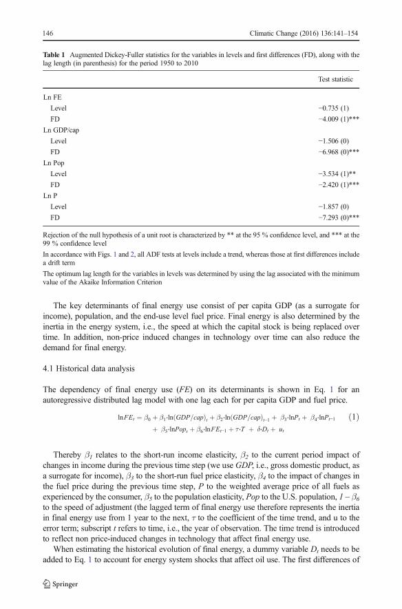
Table 1 Augmented Dickey-Fuller statistics for the variables in levels and first differences (FD), along with thelag length (in parenthesis) for the period 1950 to 2010

Test statistic

Ln FE

Level −0.735 (1)

FD −4.009 (1)***

Ln GDP/cap

Level −1.506 (0)

FD −6.968 (0)***

Ln Pop

Level −3.534 (1)**

FD −2.420 (1)***

Ln P

Level −1.857 (0)

FD −7.293 (0)***

Rejection of the null hypothesis of a unit root is characterized by ** at the 95 % confidence level, and *** at the99 % confidence level

In accordance with Figs. 1 and 2, all ADF tests at levels include a trend, whereas those at first differences includea drift term

The optimum lag length for the variables in levels was determined by using the lag associated with the minimumvalue of the Akaike Information Criterion

Climatic Change (2016) 136:141–154146

the LHS variable (final energy use) in Fig. 2b suggests that Dt could assume the value “1” in1974 (first oil shock), 1980 (second oil shock), 1991 (Gulf war), and 2008 (Global FinancialCrisis), as these drastic changes may less likely be picked up by the model. (This hypothesiswas tested and partly rejected through examining the t-statistic of each dummy variable whenestimating the model).

The single equation error correction model of Eq. 2 is an isomorphic transformation ofEq. 1 that clearly emphasizes the short-run and long-run elasticities and speed of adjustment.

ΔlnFEt ¼ α0 þ α1⋅ΔlnFEt−1 þ γ0⋅Δln GDP=capð Þt þ γ1⋅Δln GDP=capð Þt−1 þ γ2

⋅Δln GDP=capð Þt−2 þ γ3⋅ΔlnPt þ γ4⋅ΔlnPt−1 þ γ5⋅ΔlnPt−2 þ γ6

⋅ΔlnPopt þ δ⋅Dt þ τ ⋅T þ ϕ⋅ lnFEt−1 þ β1

ϕ⋅ln GDP=capð Þt−1 þ

β2

ϕ⋅lnPt−1 þ β3

ϕ⋅lnPopt−1

� �þ ut

ð2ÞEquation 2 describes the equilibrium relationship between the first differences of the

logarithm in final energy (ln FEt – ln FEt-1) and those of its lagged term along with the firstdifferences of the other right hand side variables from Eq. 1 and the lagged term of their levels.A change in any of the first-differenced (and stationary) right hand side variables causes animmediate change in the first-differenced (and stationary) left hand side variable, as dictated bythe respective short-run elasticities αi and γi. The error correction term then indicates the long-term adjustments of the left hand side to changes in any of the lagged variables. These will bedistributed over future time periods according to the rate of error correction or speed ofadjustment ϕ; the long-run elasticities then correspond to βi/ϕ. Hence, a given increase ine.g. GDP/cap will have an immediate short-term impact on final energy use of γ0 and anaccumulated long-term impact of β1/ϕ.

4.2 Panel data analysis

Because of the stationary characteristics of the Group 1–4 scenario outputs by both GCAMand REMIND, the intrinsic energy-economy-models’ coefficients were estimated with arelationship very similar to Eq. 1, where subscript i is added to represent the (I=26) scenarios.The dummy variable was dropped, as the temporal occurrence of shocks is impossible topredict. The resulting panel data model is given by Eq. 3.

lnFEi;t ¼ C þ α⋅ln GDP=capð Þi;t þ β⋅lnPi;t þ γ⋅lnPopi;t þ τ ⋅T þ λ⋅lnFEi;t−1 þ ui;t ð3Þ

Note that the 2010–2050 data used to estimate Eq. 3 are reported in 5-year intervals,whereas Eq. 2 can be estimated with annual observations.

5 Model estimation

5.1 Historical data analysis

Before estimating the model described by Eq. 2, the time trend was split into three differentperiods. The historical development of final energy intensity (final energy use per passenger-km) for U.S. passenger travel shows a roughly constant development from 1950 to 1964,followed by a slight increase through 1978, and a subsequent decline through 2010 (Schäfer2013). In freight transportation, energy intensity (final energy use per revenue tonne-km) hasdeclined between 1950 and 1957 but remained roughly constant thereafter (Schäfer 2013).

Climatic Change (2016) 136:141–154 147

Taking these developments into account, an additional time trend was introduced in 1957 andanother one in 1979 into Eq. 2 using dummy variables. Manual iteration for maximum R2

suggested that the first additional time trend should already be introduced in 1954 butconfirmed the 1979 introduction of the second trend.

Equation 2 was estimated with ordinary least squares for the entire 1950–2010 data series;the results are shown in Table 2. All signs are consistent with economic theory and allcoefficient estimates with the exception of the long-run multiplier of population are statisticallysignificant at least at the 95 % confidence level. The adjusted R2 results in around 0.90. Theresiduals seem to have white noise properties (normality test) and there is no evidence of serialcorrelation (Portmanteau Q test).

The short-run income elasticity of around 0.6 is slightly mitigated at any subsequent timestep t+1 and t+2, but remains positive overall. The short-run fuel price elasticity is around−0.08. Among the dummy variables, only those associated with 1974, 1980, and 1991 turn outto be significant. Jointly, the three time trends roughly reproduce the energy intensity trends

Table 2 Parameter estimates, t-statistics (in parenthesis), and regression statistics for Eq. 2 (historical data) usingannual data from 1950 to 2010

No. observations 58

α0 (Constant) 8.804 (2.28)

γ0 (Short-run elasticity: GDP/cap) 0.590 (8.80)

γ1 (L1 short-run elasticity: GDP/cap) −0.175 (−2.62)γ2 (L2 short-run elasticity: GDP/cap) −0.151 (−2.39)γ3 (Short-run elasticity: fuel price) −0.081 (−6.86)δ1974 (Dummy variable) −0.043 (−4.13)δ1980 (Dummy variable) −0.021 (−2.04)δ1991 (Dummy variable) −0.026 (−2.88)τ (Time) −0.006 (−2.33)τ1955 (Time) 0.00001 (2.37)

τ1979 (Time) −0.00002 (−6.26)ϕ (Speed of error correction) −0.078 (−2.87)β1 (Long-term effect: GDP/cap) 0.246 (3.27)

β2 (Long-term effect: fuel price) −0.026 (−3.64)β3 (Long-term effect: population) 0.267 (1.54)

Test statistics

Adjusted R2 0.9023

Root MSE 0.0084

Portmanteau Q test for 27 lags, p-value 0.9774

Normality test (Shapiro-Wilk), p-value 0.2820

Implied long-run elasticities (βi/ϕ)

GDP/cap 3.134 (4.87)

Fuel price −0.328 (−2.02)Population 3.401 (2.20)

The null hypothesis of the Portmanteau Q test for white noise is no serial correlation up to order (here) 27; thelarge p-value of 98 % suggests that the null-hypothesis cannot be rejected. The null hypothesis of the Shapiro-Wilk test is that the residuals are normally distributed; the large p-value of 28 % suggests that the null-hypothesiscannot be rejected

Climatic Change (2016) 136:141–154148

described above, i.e., a long-term decline by around 0.6 % per year with a slightly lowerintermediate (1955–1978) reduction.

The rate of error correction ϕ suggests that around 8 % of the remaining deviation fromequilibrium has been corrected in each subsequent year in response to any change in perperson GDP, fuel price, and population. The resulting long-term effects include an incomeelasticity of around 3.1, with a 95 % confidence interval ranging from 1.8 to 4.4. This elasticityaccounts for the increase in passenger and freight transportation with rising income, the shifttowards larger and more energy intensive vehicles in passenger travel and the mode shifttowards (more energy intensive) trucks in freight transportation, along with the rising relativeimportance of air travel in intercity transportation. Our estimated income elasticity is substan-tially higher than the values found in the literature for road transportation (mainly automo-biles). Based on a review of around 50 studies, Goodwin et al. (2004) derive an incomeelasticity of 1.08 (standard deviation of 0.35). The long-run fuel price elasticity turns out to bean inelastic −0.33 and compares well with the gasoline long-run price elasticities of −0.31 and−0.38 for light-duty vehicles, estimated by Small and Van Dender (2007) using 1997–2001data and 1966–2001 data, respectively. In addition, the associated 95 % confidence intervalstretches from −0.66 to 0 and is also consistent with other estimates of long-run fuel priceelasticities for passenger travel (see, e.g., Oum et al. 1990; Goodwin et al. 2004). Finally, thelong-run population elasticity turns out to be 3.4. Intuition suggests that this value should bearound unity: an extra person per household would most likely result in a less than propor-tional increase in transportation energy use as some of the additional trips are likely to beshared trips, while an extra household could lead to a roughly proportional increase intransportation energy use—an elasticity of around one. However, the lower end of the 95 %confidence interval is as small as 0.29 and the confidence interval thus includes a range of allplausible values.

5.2 Panel data analysis

Several estimation challenges exist with respect to the dynamic panel data model in Eq. 3. Theerror term ui,t can be decomposed into unobserved individual level effects (that are indepen-dent of time) and observation specific errors. First-differencing Eq. 3 then removes theunobserved individual level effects, and therefore eliminates the omitted variable bias in themodel estimation. However, differencing the predetermined variables Fi,t-1 makes them en-dogenous because the first differenced observation specific errors are correlated with the first-differenced Fi,t-1, thus violating the requirement for strict exogeneity. Ordinary least squaresestimators would thus be biased. Therefore we use the estimator developed by Arellano andBond (1991) that is derived from the Generalized Method of Moments and instruments thosedifferenced variables that are not strictly exogenous with their available lags.

Table 3 summarizes the regression results of the panel data models, which were estimatedwith 2010–2050 data from all Groups 1–4. The sign of all coefficients is consistent witheconomic theory and all coefficients are highly significant. The null hypothesis of the Waldstatistic (all coefficients except the constant are zero) is clearly rejected. For comparison, thelong-run results estimated from Eq. 2 based on the entire time horizon 1950–2010 data are alsoshown.

The elasticity of the lagged dependent variable (λ) of GCAM and REMIND over a 5-yearperiod results in 0.542 and 0.504, respectively. Although both coefficients are slightly lowerthan that implied in the annual historical (1950–2010) dataset over 5 years of (1–0.078)5=0.666, thus suggesting a slightly smaller inertia compared to that observed historically, they arestill within the confidence interval of the latter. The roughly comparable inertia and thus speed

Climatic Change (2016) 136:141–154 149

of error correction of the model outputs to those underlying the historical data accumulatedover 5 years would imply comparing the long-run elasticities of the annual historical data tothe short-run elasticities of the panel data model. However, because the long-run elasticitiesreflect the consumer and industry responsiveness in transportation energy use to changes inany of the RHS variables to have fully materialized, we also compare these estimates for boththe historical and the projected data.

The intrinsic short- and long-run income elasticities of both energy-economy-models aresignificantly smaller than that observed historically, a fact we already observed when com-paring the historical increase in final energy use to the projected levels of GCAM andREMIND in Fig. 1a. As already suspected from Fig. 1a, the income elasticity of REMIND(0.300[short-run: SR], 0.606[long-run: LR]) is larger than that of GCAM (0.158[SR],0.345[LR]).

In contrast, the intrinsic short- and long-run price elasticities of both energy-economy-models are within the 95 % confidence interval of the long-run elasticity (of −0.327) estimatedusing the 1950–2010 time series. Thereby, the intrinsic price elasticity of the REMIND model(−0.257[SR], −0.519[LR]) turns out to be larger than that of GCAM (−0.125[SR],−0.272[LR]). The intrinsic short- and long-run population elasticities of GCAM and REMINDare also plausible and within the confidence interval of the rather large estimate of thehistorical data.

The estimated time coefficient of around 0.5 % autonomous reduction of final energy useper year (0.5 % for GCAM and 0.4 % for REMIND) is slightly smaller than those estimatedover the historical time period of 0.6 % per annum but well within the confidence interval of

Table 3 Parameter estimates, z-statistic (in parenthesis), and regression statistics for Eq. 3 (dynamic panel data)compared with key results from Table 2 (with t-statistics in parenthesis)

GCAM 2010–2050 REMIND 2010–2050 Historical 1950–2010

No. Observations 182 182 58

Freq. of observations (years) 5 5 1

α0 (Constant) 6.730 (14.21) 3.058 (5.35) 8.804 (2.28)

α (Income elasticity) 0.158 (9.58) 0.300 (11.64) 0.590(1) (8.80)

β (Fuel price elasticity) −0.125 (−8.55) −0.257 (−16.99) −0.082 (−6.86)γ (Population elasticity) 0.644 (16.15) 0.674 (13.70) 0

τ (Time, in %/yr) −0.005 (−14.80) −0.004 (−7.87) −0.006 (−2.33)λ (Elasticity of lagged dependent variable) 0.542 (9.94) 0.504 (9.89)

ϕ (Error correction rate) −0.078(2) (−2.87)Implied long-run

α (Income elasticity) 0.345 (12.28) 0.606 (11.71) 3.134 (4.87)

β (Fuel price elasticity) −0.272 (−12.16) −0.519 (15.64) −0.327 (−2.02)γ (Population elasticity) 1.405 (12.73) 1.360 (7.61) 3.401 (2.20)

Test statistics

R2 0.9023

Wald χ2 3492.3 3682.4

Both dynamic panel data models were estimated with the Arellano-Bond estimator

The reported Error Correction Model (ECM) coefficients are long-run elasticities(1) At time t only; see Table 2 for those at t-1 and t-2(2) After 5 years, the implied elasticity of the lagged dependent variable would result in (1–0.078)5 =0.666

Climatic Change (2016) 136:141–154150

the latter. (For GCAM, the estimated autonomous reduction of final energy use of0.5 % per year is identical to the exogenously imposed autonomous reduction of finalenergy intensity; similarly, the inputs into the production functions underlying theREMIND model are reduced by scaling factors that change over time and theweighted average of these scaling factors results in our estimated 0.4 % decline intransportation sector final energy use). Between the two energy models, price elastic-ity and autonomous improvements seem to trade. Reductions of final energy use resultto a larger extent from non-price induced changes in GCAM and due to a largersensitivity to price changes in REMIND.

Figure 3 compares the 95 % confidence intervals of the estimated long-runelasticities from the 1950–2010 historical development and the short- and long-runcoefficients from both GCAM and REMIND. In addition, literature survey-based95 % confidence intervals related to road transportation (mainly automobiles) areshown, which also include other countries than the U.S. (Goodwin et al. 2004). Ascan be seen, the short- and long-run elasticity-based confidence intervals of the twoenergy-economy-models overlap with all those underlying the historical developmentand the literature survey-based studies, except for the income elasticity. There, theshort-run elasticities of GCAM and REMIND are outside the 95 % confidenceintervals of both the literature survey-based study and our historical estimate. How-ever, these models’ intrinsic long-run elasticities still overlap with the confidenceinterval of the literature-based study, which itself is not within the confidence intervalof our own estimate using the historical U.S. data. This apparent inconsistency maysuggest that our own estimate of the long-run income elasticity with respect to finalenergy is at the higher end.

Fig. 3 Ninety five percent confidence intervals of the coefficient estimates: income elasticity (α), fuel price elasticity(β), population elasticity (γ), the time trend (τ), and coefficient of lagged dependent variable (λ). The source for theliterature-survey based intervals (around 50 studies) is Goodwin et al. (2004). SR: short-run; LR: long-run

Climatic Change (2016) 136:141–154 151

6 Interpretation of the results

The most striking difference between the estimated intrinsic elasticities of the GCAM andREMIND models and the historical development is the comparatively small intrinsic incomeelasticity of both models. (In light of the recently introduced tight fuel economy standards forlight-duty vehicles, such lower income elasticity of fuel use seems plausible; however, asdescribed below, both models did not include these new tight regulations and therefore weexamine this discrepancy in more detail). In addition, the REMIND model incorporates aslightly larger price elasticity than GCAM. Here we attempt to interpret these differencesthrough the key assumptions and characteristics underlying each energy-economy-model.

6.1 Income elasticity

In GCAM, the transportation sector is implemented on the service level (passenger-kilometerstraveled and tonne-kilometers generated) and driven by exogenous, scenario-specific growth inpopulation and GDP, and endogenous generalized transportation costs (Kyle and Kim 2011);the latter are expressed as travel money expenditures plus the ratio of the value of time (as apercentage of the wage rate) and average travel speed. For the 26 scenarios examined,passenger-kilometers traveled and tonne-kilometers generated double at most, with the excep-tion of one freight transport projection in one of the baseline (Group 1) scenarios. Thecomparatively modest projected growth in passenger travel partly results from the assumedhigh value of time, being 100 % of the wage rate. The time cost component of the generalizedcost term then corresponds to the ratio of wage rate and average travel speed. As the wage ratecontinues to rise with per person GDP at a higher rate than the average speed, travel costsincrease and therefore depress travel demand. A lower value of time would reduce thesignificance of the time cost term compared to the economic cost component and thereforeresult in a stronger growth in passenger transportation demand.

Another GCAM-related important reason for the comparatively low income elasticity withrespect to final energy use is a modestly stringent CAFE standard, tightening average light-duty vehicle fuel economy levels from a stock average of about 20 miles per gallon (MPG) in2005 to 24 MPG in 2020 and 26 MPG in 2035.

The transport sector of REMIND is the hybrid of a linear energy systems model and amacroeconomic production function. The linear energy systems model converts final energyinputs into energy services (mobility) for competing transportation modes, using vehicle-specific efficiencies and capital costs. At the same time, each mode represents an input factorto the constant elasticity of substitution (CES) production function representing the totalmobility produced. The ability for mode substitution is determined by a substitution elasticityof 1.5. The total “value of transport” is then input into a rather inflexible CES nest (substitutionelasticity of 0.3) and substitutes with stationary energy use to produce an “aggregate energy”good that itself is input to the topmost CES-function combining capital, labor and theaggregate energy good to produce GDP (Luderer et al. 2013). The individual inputs into thenested CES production function have time-dependent CES-efficiency parameters, leading to atime-dependent reduction of final energy demand. Thereby the efficiency parameters arecalibrated in such a way that the model in standard configuration reproduces an externalbaseline scenario (Pietzcker et al. 2014).

The assumptions underlying the baseline scenario and its implementation are a major factoraffecting the comparatively low income elasticity of transport sector final energy use for theU.S. in REMIND. Historical per-capita transport final energy use levels in the U.S. are higherby a factor of 2–3 compared to those seen in most other parts of the world at similar per-capita

Climatic Change (2016) 136:141–154152

income levels. The REMIND baseline scenario assumes that the future U.S. development willpartially converge to other regions because of a number of factors, including i) a change in theexpectations about future oil prices, leading to a renewed effort to decrease oil demand fromtransport; ii) increased development and use of high-efficiency vehicles driven by stringentefficiency standards implemented both abroad and in the U.S.; iii) congestion effects inmetropolitan areas limiting further mobility growth, and iv) increased public transport infra-structure and stronger city planning, reducing the ultimate dependence on light-duty vehicles.This assumed international convergence underlying the REMIND model entails a slowreduction of per-capita transport energy demand in the U.S., which in combination with theassumed continued GDP growth leads to the described low implicit income elasticity.

6.2 Price elasticity

The intrinsic price elasticity in GCAM is determined by the assumed price elasticities of theenergy service demands, and by the model’s ability to substitute more fuel-efficient transpor-tation modes and technologies for existing ones. In the passenger transport sector, future modeshares are determined primarily by the income-driven value of time, and as such tend to becomparatively less responsive to changes in energy prices. In contrast, REMIND simulates astronger responsiveness to changes in fuel prices because the value of time is not explicitlyincluded in the determination of demand for transportation. Accordingly, fuel costs make up alarger share of total travel costs, and a change of fuel costs thereby leads to a larger change oftotal travel costs compared to GCAM. This effect, in combination with the possibility of i)substituting modes for one another (see discussion in the income elasticity section above) andii) reducing the demand for transport energy services in the “aggregated energy” CES nest asthe relative price of mobility increases, leads to the observed responsiveness to fuel prices inREMIND. In both models, the adoption of fuel-saving and alternative fuel technologiesdepends on the specified set of alternative technologies that becomes available over time,and constraints that limit the rate of penetration of and thus substitution for existing technol-ogies. These are also important assumptions that can strongly affect the price elasticity andwould need to be studied carefully.

7 Conclusions

This paper presented an econometric approach to validating energy-economy-models, namelyusing a large number of model scenario outputs to estimate aggregate price- and incomeelasticities with the help of linear dynamic panel data models. We compared these models’intrinsic elasticities with one another and those based on historical data.

Both energy-economy-models behave broadly similar with respect to transportation finalenergy use. They also compare well to the elasticities associated with the long-term historicaldevelopment of the U.S. transportation sector and a survey of around 50 studies from variouscountries, thus generating confidence in the way the models behave. The only noticeabledifference to historical observations and those from other studies is their comparatively lowincome elasticity.

The lower responsiveness of final energy use with respect to changes in income can beexplained mainly by assumptions underlying each of the energy-economy-models, namely therising importance of the value of time for transport decisions in GCAM, and the assumeddeceleration of transport energy demand growth in REMIND due to fuel efficiency standards,congestion effects, and improved city planning and public transport infrastructure. Because

Climatic Change (2016) 136:141–154 153

such differences in income elasticity to the historical value can lead to widely different levelsin final energy use and CO2 emissions, especially over the very long (close to 100 years) timehorizon that underlies such energy-economy-models, the need for a careful evaluation of someof these assumptions becomes apparent.

The approach pursued here can be applied to more variables of the transportation sector.Estimating CO2 emissions as a function of primary energy use, carbon prices, etc. would be alogical next step. In addition, this approach could be extended to more sectors and ultimatelyentire energy-economy-models.

Open Access This article is distributed under the terms of the Creative Commons Attribution License whichpermits any use, distribution, and reproduction in any medium, provided the original author(s) and the source arecredited.

References

Arellano M, Bond S (1991) Some tests of specification for panel data: Monte-Carlo evidence and an applicationto employment equations. Rev Econ Stud 58:277–297

Beckman J, Hertel T, Tyner W (2011) Validating energy-oriented CGE models. Energy Econ 33:799–806Energy Modeling Forum (EMF) (1977) Energy and the Economy, EMF Report 1, Volume 1, September 1977,

Stanford, CA. http://emf.stanford.edu/files/pubs/22407/1v1.pdfGoodwin P, Dargay J, Hanly M (2004) Elasticities of road traffic and fuel consumption with respect to price and

income: a review. Transp Rev 24:275–292Kriegler E, Mouratiadou I, Brecha RJ, Calvin K, De Cian E, Edmonds J, Kejun J, Luderer G, Tavoni M,

Edenhofer O (this issue) Will economic growth and fossil fuel scarcity help or hinder climate stabilization?Overview of the RoSE multi-model study. Climatic Change.

Kyle P, Kim SH (2011) Long-term implications of alternative light-duty vehicle technologies for globalgreenhouse gas emissions and primary energy demands. Energy Policy 39:3012–3024

Luderer G et al (2013) Description of the REMIND Model (Version 1.5). http://www.pik-potsdam.de/research/sustainable-solutions/models/remind/description-of-remind-v1.5

Oum TH, Waters WG, Yong JS (1990) A survey of recent estimates of price elasticities of demand for transport.The World Bank, Infrastructure and Urban Development Department

Pietzcker RC, Longden T, Chen W, Fu S, Kriegler E, Kyle P, Luderer G (2014) Long-term transport energydemand and climate policy: alternative visions on transport decarbonization in energy-economy models.Energy 64:95–108

Schäfer A (2013) Transportation demand, technological change, and energy use in the U.S. transportation sectorsince 1900. Draft paper. Precourt Energy Efficiency Center, Stanford University

Schäfer A, Heywood JB, Jacoby HD, Waitz IA (2009) Transportation in a climate-constrained world. The MITPress, Cambridge

Schwanitz VJ (2013) Evaluating integrated assessment models of global climate change. Environ Model Softw50:120–131

Small KA, Van Dender K (2007) Fuel efficiency and motor vehicle travel: the declining rebound effect. Energy J28(1):25–51

Wilson C, Grübler A, Bauer N, Krey V, Riahi K (2013) Future capacity growth of energy technologies: arescenarios consistent with historical evidence? Clim Chang 118:381–395

Climatic Change (2016) 136:141–154154