Scuola Internazionale Superiore di Studi Avanzati - Trieste

Exploring Language Mechanisms: The Mass-Count Distinction and The Potts Neural

Network

Ritwik KulkarniCognitive Neuroscience

SISSA

Supervisor:Prof. Alessandro Treves

Thesis submitted for the degree of Doctor of Philosophy

Trieste, 2014

SISSA - Via Bonomea 265 - 34136 TRIESTE - ITALY

Abstract

The aim of this thesis is to explore language mechanisms in two aspects. First, the statisticalproperties of syntax and semantics, and second, the neural mechanisms which could be of possibleuse in trying to understand how the brain learns those particular statistical properties. In the firstpart of the thesis (part A) we focus our attention on a detailed statistical study of the syntax andsemantics of the mass-count distinction in nouns. We collected a database of how 1,434 nouns areused with respect to the mass-count distinction in six languages; additional informants characterisedthe semantics of the underlying concepts. Results indicate only weak correlations betweensemantics and syntactic usage. The classification rather than being bimodal, is a graded distributionand it is similar across languages, but syntactic classes do not map onto each other, nor do theyreflect, beyond weak correlations, semantic attributes of the concepts. These findings are in linewith the hypothesis that much of the mass/count syntax emerges from language- and even speaker-specific grammaticalisation. Further, in chapter 3 we test the ability of a simple neural network tolearn the syntactic and semantic relations of nouns, in the hope that it may throw some light on thechallenges in modelling the acquisition of the mass-count syntax. It is shown that even though asimple self-organising neural network is insufficient to learn a mapping implementing a syntactic-semantic link, it does however show that the network was able to extract the concept of 'count', andto some extent that of ‘mass’ as well, without any explicit definition, from both the syntactic andfrom the semantic data.

The second part of the thesis (part B) is dedicated to studying the properties of the Potts neuralnetwork. The Potts neural network with its adaptive dynamics represents a simplified model ofcortical mechanisms. Among other cognitive phenomena, it intends to model language productionby utilising the latching behaviour seen in the network. We expect that a model of languageprocessing should robustly handle various syntactic- semantic correlations amongst the words of alanguage. With this aim, we test the effect on storage capacity of the Potts network when thememories stored in it share non trivial correlations. Increase in interference between storedmemories due to correlations is studied along with modifications in learning rules to reduce theinterference. We find that when strongly correlated memories are incorporated in the storagecapacity definition, the network is able to regain its storage capacity for low sparsity. Strongcorrelations also affect the latching behaviour of the Potts network with the network unable to latchfrom one memory to another. However latching is shown to be restored by modifying the learningrule. Lastly, we look at another feature of the Potts neural network, the indication that it may exhibitspin-glass characteristics. The network is consistently shown to exhibit multiple stable degenerateenergy states other than that of pure memories. This is tested for different degrees of correlations inpatterns, low and high connectivity, and different levels of global and local noise. We state some ofthe implications that the spin-glass nature of the Potts neural network may have on languageprocessing.

Acknowledgement

The journey towards completing this thesis has seen a lot of ups and downs but fortunatelythere has been enough 'adaptation' for the dynamics to 'latch' from one valley to another withoutbeing stuck in a minima for too long. First and foremost, I would like to thank my supervisorAlessandro Treves who gave me the opportunity to follow my scientific drives and allowed me tocomplete my thesis. His persuasion of objective thinking and scientific rigour has taught me how toapproach a problem and not to leave any stone unturned in finding the answers. I thank him for hissupport in a very testing phase of my life. I am grateful for the freedom of thought and in general,freedom of life, on occasions too much, that I received from him.

I am indebted to all the informants (Giusy, Gayane, Kamayani, Tejaswini and many more)who provided the linguistic data to me with a lot of enthusiasm. The mass-count project would nothave been possible without them.

I would like to thank Susan Rothstein for her collaboration on the mass-count project andher invaluable linguistic insights.

I would also like to thank Giosue Baggio, the discussions and debates in the meetingorganised by him have been of great value to me. They were especially fun in summer when wegathered in the SISSA garden to talk science. I had the opportunity to learn from computationallinguists at ILLC, Amsterdam. It was a great experience for me and I thank Prof Rens Bod for that. Iam thankful to the faculty of the Cognitive Neuroscience Sector for their support in a toughsituation.

I thank the examiners who have set aside time from their busy schedules to read my thesisand giving very valuable comments.

Our student secretariats (Riccardo and Federica) have been life savers when it came topreventing foreign students like me to fall into a bureaucratic nightmare.

Life would have been monochromatic and dry if it wasn't for the friends that I shared my 4years with. Besides scientific discussions any and everything under the sky was up for intense,enlightening and fruitful debates that lasted late into the nights. Sahar, my labmate was an importantsource of cheer in our shared troubles. I will not forget the times I went with Amanda and herfamily into Croatian forests, looking for bears. I have fond memories of sometimes happy,sometimes crazy and sometimes adventurous moments with Federica, Jenny , Ana Laura, Naeem,Stefania, Arash, Athena, Sina, Georgette, Giovanni, Milad, Indrajeet, Wasim, Iga, Ana and manymore. My LIMBO lab-mates have been very interesting people and good models of complexsystems. My friends back home in India (Pradeep, Sanket, Swapnil, Shirish, Rohan, Gayu, Rekha,Prasanna, Amey, Aditi, Juzar, Gauri, Sanjay, Prateek, Yash, Sahil) too have made my life happierwith their long distance stupidity.

I am immeasurably grateful to my family (Aai, Richa, Amit) for their undying selflessencouragement and support. I dedicate this thesis to my father, Dilip, who was a constant source ofjoy, motivation, intelligence and inspiration but had to unfortunately bid us goodbye midway.Saylee had to bear with a lot of my off-normal deviations and has been a constant loving andsupporting companion. My journey of completing the thesis wouldn't have been the same withouther.

In the loving memory of my father...

Table of Contents

1 General Overview............................................................................................................................1

Chapter 2.............................................................................................................................................5

2.1 Introduction:...................................................................................................................................5

2.2. Methods.......................................................................................................................................10

2.2.1. Data Collection....................................................................................................................10

A) Noun List.............................................................................................................................10

B) Usage Tables........................................................................................................................10

C) Semantic Table.....................................................................................................................12

2.2.2. Analysis................................................................................................................................13

A) Hamming Distance Scale.....................................................................................................13

B) Clustering and Information Measures..................................................................................16

C) Artificial Syntactic String Generation..................................................................................18

2.2.3. Corpus Study of the Mass/Count Distinction in English.....................................................19

2.3. Results.........................................................................................................................................21

2.3.1. Individual Syntactic Rules and Semantic Attributes Do Not Match...................................21

2.3.2. Hamming Distance..............................................................................................................28

2.3.3. Mutual Information along the Main Mass/Count Dimension..............................................32

2.3.4. Mutual Information across the Complete Syntactic Classification.....................................36

2.3.5. CHILDES Corpus Study......................................................................................................41

2.4. Discussion:..................................................................................................................................44

Appendix A.........................................................................................................................................51

Chapter 3...........................................................................................................................................58

3.1 Motivation and a brief summary:.................................................................................................58

3.1.1 Introduction:.........................................................................................................................58

3.1.2 Network modelling:..............................................................................................................59

3.2 The network:.................................................................................................................................60

A) Classification of nouns:............................................................................................................60

B) Classification of markers:.........................................................................................................61

3.3 Categorisation of markers:...........................................................................................................64

3.4 Categorization of nouns:..............................................................................................................67

3.5 The syntax-semantics interaction:................................................................................................71

3.5.1 Quick summary of information measures:...........................................................................71

3.5.2 Processed Interacting Mutual Information:..........................................................................73

A) The effect of competition strength:...........................................................................................73

B) Combined learning of syntax and semantics:......................................................................74

3.6 Discussion:...................................................................................................................................76

Appendix B.........................................................................................................................................79

Chapter 4...........................................................................................................................................83

Section I

A] Introduction:..................................................................................................................................83

B) Types of neural networks:..............................................................................................................83

C) The Potts neural network model for cortical dynamics:................................................................87

............................................................................................................................................................90

D) Latching behaviour:.......................................................................................................................90

E) Application of the Potts neural network to language:....................................................................91

Section II

4.1 Introduction:.................................................................................................................................93

4.1.1 Importance of correlations in neuronal representations:......................................................93

4.1.2 A brief summary:..................................................................................................................94

4.1.3 On ultrametricity:..................................................................................................................96

4.2 Correlations in patterns:...............................................................................................................97

4.2.1 Pattern generation:................................................................................................................97

4.2.2 Scatter of correlations:..........................................................................................................99

4.3 Storage capacity:........................................................................................................................101

4.4 Signal and noise:.........................................................................................................................104

4.5 Retrieval behaviour above storage capacity:..............................................................................107

4.6 Storage capacity with correlated retrievals:................................................................................110

4.7 Modification of learning rules:...................................................................................................112

4.7.1 'Popularity' subtraction:.......................................................................................................112

4.7.2 Constrained synaptic modification:....................................................................................113

4.7.3 Effect of modified learning rule on noise profile:..............................................................114

4.8 Storage capacity with modified learning rule:............................................................................116

4.9 A self-excitation trick to store more patterns:.............................................................................118

4.10 Discussion:................................................................................................................................119

Section III

4.11 On the glass phase of the Potts Neural network:......................................................................121

4.11.1 Suggestions from the mean field models of the spin glass phase:....................................122

4.11.2 Glass phase in the Potts neural network model:...............................................................123

4.12 Indication of spin glass phase in the 'cortical' Potts model:.....................................................124

4.13 Effect of local module temperature:.........................................................................................128

4.14 Effect of network level noise:...................................................................................................131

4.15 Behaviour at low S and full connectivity:................................................................................134

4.16 Brief Discussion:......................................................................................................................136

5 A Report on the Effect of Learning Rules on Latching Dynamics..........................................138

5.1 Latching behaviour for increased correlation between patterns............................................138

5.2 Effect on latching due to different learning rules:.................................................................139

6 Conclusions..................................................................................................................................147

Future Directions............................................................................................................................150

Bibliography....................................................................................................................................151

Publications.....................................................................................................................................157

List of Figures

Figure 2.1: Schematic representation of the Hamming distance scale....15Figure 2.2: MI across languages remains low, however it is measured....25Figure 2.3: Distribution of nouns along the mass/count dimension....29Figure 2.4: The distribution for Marathi, restricted to concrete and to abstract nouns...29Figure 2.5: Distribution of nouns on the main mass/count dimension for semantics...30Figure 2.6: Scatter plots of variance values along the main mass/count dimension...31Figure 2.7: Scatter plots of mutual information values along the main mass/count dimension...34Figure 2.8: Scatter plots comparing variance with mutual information values... 35Figure 2.9: The entropy scales up with the number of questions...37Figure 2.10: Scatter plots of mutual information values for abstract and concrete nouns...38Figure 2.11: Scatter plots comparing mutual information on the MC dimension with total mutual informationvalues...39Figure 2.12: Mutual information between language pairs vs. artificially generated control values...40Figure 2.13: Distribution of nouns from the CHILDES corpus on the main mass/count dimension...42Figure 2.14: Visualization of the nouns in the Brown’s section of CHILDES corpus in three dimensions, frommulti-dimensional scaling....44Figure A7- correlation between syntactic questions....54Figure A9- Exponential fit to MC-dimension distributions...56

Figure 3.1. Schematic diagram of the artificial neural network...61Figure 3.2. Correlograms for 784 concrete nouns in each of the 6 languages in our study...64Figure 3.3. Correlograms for 650 abstract nouns...65Figure 3.4. Correlogram of semantic markers for concrete nouns...66Figure 3.5. Position of 784 concrete nouns in the output space as defined by 3 output units...68Figure 3.6. Histogram of nouns in reference to Figure 3.5...68Figure 3.7. Position of 650 abstract nouns in the output space as defined by 3 output units...70Figure 3.8. Histogram of nouns in reference to Figure 3.8...70Figure 3.9. Variation of the output entropy to input entropy ratio for different values of the competition strength, T...74

Figure 3.10. Mean normalised mutual information at various γ

values for concrete nouns in 6 languages

when N=3 output units, ...75Figure B1- Log plots related to figure 3.6 and 6.8...79Figure B2- Convergence of weight matrix during learning...80

Figure A: A schematic representation of an autoassocitive network with recurrent connections...85Figure B: Energy landscape depicting attractor dynamics...86Figure C: Conceptual visualisation of the Potts model, with local patches represented by S state interconnected units, forming a global cortical network...87Figure D: Latching behavior of the Potts network....91Figure E: Potts network applied to BLISS ...92

Figure 4.1 Schematic representation of the pattern generation algorithm...98Figure 4.2a: Scatter Plots showing the spread of pairwise correlations amongst patterns for a<0.6 ...100

Figure 4.2: b Same pairwise correlation scatter as above but for 0.6⩽a⩽0.9 ...101

Figure 4.3: Storage Capacity as a function of sparsity ...102Figure 4.4: Standard deviation of the noise profile as a function of sparsity....105Figure 4.5: Standard deviation and noise as a function of storage load...107Figure 4.6: Correlation scatter with an overlay of the three types of retrieval behaviours...108Figure 4.7: Storage Capacity when the strong correlations are incorporated in the definition of storage capacity...104Figure 4.8: Reduction in standard deviation and skewness (as a function of sparsity) brought about by the modification of the learning rule, LR2 and LR3...115Figure 4.9: Reduction in standard deviation and skewness (as a function of storage load) brought about by the modification of the learning rule, LR2 and LR3...116Figure 4.10: Storage capacity as a function of sparsity for the three learning rules LR1, LR2 and LR3...117Figure 4.11: Storage capacity when signal is boosted by self reinforcement (w=0.8)...126

Figure 4.12: Energy states for pure patterns and network state....119Figure 4.13: Mean difference in energy between network state and pure pattern...127Figure 4.14: Mean difference in energy, for three different values of , in random patterns...129Figure 4.15: Mean energy difference for three levels of local noise, in low correlation patterns....130Figure 4.16: Mean energy difference for three levels of local noise, in high correlation patterns....131Figure 4.17: Fraction of patterns successfully retrieved as a function of external noise (random patterns)...132Figure 4.18: Influence of external noise on the total Mean difference in energy...133Figure 4.19: Fraction of patterns successfully retrieved as a function of external noise (low correlation patterns)...134Figure 4.20: Mean difference in energy, for different S and Cm...135

Figure 5.1: Latching statistics for high correlation patterns using the learning rules LR1, LR2 and LR3...140

Figure 5.2: (i),(ii) and (iii): Latching transitions using LR1, LR2 and LR3...142,143.

Figure 5.3: Latching statistics for low correlation patterns using the learning rules LR1, LR2 and LR3...144

Figure 5.4: Latching statistics for random correlation patterns using the learning rules LR1, LR2 and LR3...145

List of Tables

Table 2.1: List of questions used in English to compile the usage table...11Table 2.2: Questions used to probe the semantic properties of the nouns...12Table 2.3: A small section of the usage table for English as filled by a native informant..14Table 2.4: A case of relatively high correspondence between a semantic attribute and a syntactic rule..23Table 2.5: The correspondence between languages is not higher...24Table 2.6: Congruency and mutual information between languages...27Table 2.7: Language–entropy relations....33Table 2.8: Entropy values for the full classification in the 2.6 languages, and for semantics...37Table 2.9: Variance of the markers in the CHILDES corpus...43Table A1: List of questions used in Armenian to compile the usage table...51Table A2: List of questions used in Hebrew to compile the usage table...52Table A4: List of questions used in Italian....53Table A5: List of questions used in Marathi...53Table A6- Fraction of 'yes' answers to syntactic-semantic questions...54

Table A7- Subgroups at each hamming distance...56

Table B3- Correlation between self-organised groups and MC-dimension groups...81

Table 4.1a: Mean Correlation, N as , for Successful Pattern Pairs, case (i)...109

Table 4.1b: Mean Correlation, Nas , for Failed Pattern Pairs of case (ii)...109

Table 4.1c: Mean Correlation, Nas , for Failed Pattern Pairs of case (iii)...110

1 General Overview

One of the epitomes of cognitive function is the ability to communicate through a language.

The formal study of language has a long history with one of the earliest works dating back to 500

BCE when Panini studied Sanskrit. Humans are thought to be the only species that exhibit such a

high level of complexity and structure in their communication, which far exceeds the few other

species that show, to some extent, a developed communication ability like songbirds [van

Heiningen et al 2009] and cetaceans like Killer Whales [Deecke et al 2009]. These species have a

limited set of 'symbols' and rely mostly on repetition of sequences to communicate. The marked

difference in the human languages is the possibility to combine symbols in different ways to convey

different meanings, and possibly construct infinite set of unique sentences. It is still unclear why

there is a sudden leap in human communication abilities despite sharing similar neural mechanisms

to other species [Fisher, Marcus 2006].

Language processing can be investigated in several aspects, including A) The structure and

rules of a language, which entails the study of syntax and semantics, and B) The encoding of those

rules in the brain through neural mechanisms.

Several proposals have been made in the quest to explain language acquisition in humans.

'Generativism' was one of the earlier ideas in the 1980's and its initial formulation proposed that

humans are born with biological constraints on their knowledge of linguistic principles and as the

child grows, syntactic cues from the environment set certain features in the child's syntactic

repertoire, thus bringing about complete language acquisition [Chomsky, 1980; Baker, 2002]. This

view was challenged by the 'empiricism' idea which argues that in the light of lacking

neuroscientific evidence to find a specific language acquisition device as proposed in generitivism,

language is rather an emergent phenomenon developed through language use [Tomasello 2003;

O'Grady 2008]. In relation to this, statistical models of language learning emerged, which suggest

that a child can extract rules and structure from the statistics of the inputs it receives and thus is able

to acquire the required knowledge to use the language [Saffran 2003; Lany, Saffran 2010].

Statistical models of language learning extend to connectionist models, which try to explore

the mechanisms by which language can be encoded in the connections between neurons and make

use of the general cognitive principles of learning. Several attempts have been made at modelling

the brain mechanisms that would subserve language processing [SRN-Elman 1991; LISA-Hummel,

1

Holyack 1997; Neural Blackboard Architecture-Velde, de Kamps 2006]. All these models provide a

conceptual basis and requirements (like learning with distributed representations, self-organisation

and the combinatorial property of syntax) for a neural architecture to support language processing

but fall short in satisfying a realistic upward scaling of a natural language (eg. LISA) or require

specifically pre-organised structure (eg. Neural Blackboard Architecture). An important aspect

however is the ability of a neural network to learn from the statistics of a natural language. An

attempt at artificially simulating statistical relations between words and syntactic categories was

presented in BLISS [Pirmoradian, Treves 2011] and a neural network modelling cortical dynamics

was tested in its ability to 'acquire' the statistical relationships. All such models show promise to

some extent, however also highlight the enormous challenge and difficulty in approaching

anywhere near the full requirements of a natural language.

In this thesis we focus our attention (in part A) on the statistical properties of 6 natural

languages in the domain of the mass-count distinction in nouns. The mass-count distinction as

explained in chapter 2 has been subject to intense debate for several decades and is particularly

interesting to us, due to its perceived intuitive relation between syntax and semantics, which is also

linked to the cognitive perception of nouns. We make a detailed cross linguistic study on the

information obtained from the native speakers of the 6 languages and probe the statistical

relationship between syntax and semantics of the mass-count nouns. Further, in chapter 3 we test

the ability of a simple neural network to learn the syntactic and semantic relations of nouns, in the

hope that it may throw some light on the challenges in modelling the acquisition of the mass-count

syntax.

In part B we study properties of the Potts neural network, regarding its storage capacity and

the spin glass phase. The Potts neural network is a simplified model of cortical dynamics and its

dynamical behaviour exhibits some interesting features like latching between attractor states

[Kropff, Treves 2006; Russo, Treves 2012]. The model was studied in its ability to produce

sentences from BLISS [Pirmoradian, Treves 2012], however the correlations between words in a

sentence was kept low to study the basic behaviour of the network. In chapter 4-section II we look

at why correlations are important and a necessary requirement for a language processing model and

then study the effects of increased correlations amongst stored memories in the Potts network.

Lastly in section III of chapter 4 we look at an interesting observation, namely the spin glass phase

of the Potts neural network. We describe what a spin glass phase is and look at the indications that

2

the Potts neural network is operating in the spin glass phase. The possible implications of which are

discussed in the conclusions.

3

Part A

Statistical study of natural languages: The Mass-Count

Distinction

4

Chapter 2

A Statistical Investigation into the Cross-Linguistic Distribution of Mass and Count Nouns: Morphosyntactic and Semantic Perspectives

2.1 Introduction:

The mass/count distinction between nouns, in various languages, has been discussed in the

linguistic literature since [Jespersen 1924], and has received considerable attention in particular in

the last 35 years [see the bibliography in Bale & Barner 2011]. This distinction between mass and

count nouns is a grammatical difference, which is reflected in the syntactic usage of the nouns in a

natural language, if it makes the distinction at all (as has been often noted, not all language do; in

the Chinese language family, for example, all nouns are mass). For example, in English, mass nouns

are associated with quantifiers like little and much and require a measure classifier (kilos, boxes)

when used with numerals; on the other hand, count nouns are associated with determiners like a(n),

quantifiers like many/few or each, and can be used with numerals without a measure classifier.

These syntactic properties are intuitively correlated with semantic properties. Typical count

nouns denote sets of individual entities, as in girl, horse, pen, while typical mass nouns denote

‘substances’ or ‘stuff’, for example, mud, sand, and water. It has often been noted that the

correlation is not absolute, and that there are mass nouns which intuitively denote sets of

individuals (e.g., furniture, cutlery, footwear). Nonetheless, the correlation seems non-arbitrary and

there has been much discussion of this correlation in the linguistics literature as well as in the

psycholinguistics literature [e.g., Soja et al. 1991, Prasada et al. 2002, Barner & Snedeker 2005,

Bale & Barner 2009] and in the philosophical literature [e.g., Pelletier 2011 and references cited

therein].

5

Within the semantics literature, a seminal attempt to ground the syntactic distinction

semantically is [Link, 1983]. Link proposed that mass nouns are associated with homogeneity and

cumulativity, while count nouns are associated with atomicity. Homogeneity, cumulativity, and

atomicity are properties which can be associated with matter or with predicates. An object is atomic

when it has a distinguishable smallest element which cannot be further divided without

compromising the very nature of the object, and an atomic predicate denotes a set of atomic

elements. Thus boy is an atomic predicate, since we can easily identify atomic boys, parts of which

do not count as boys. Homogeneity is a property by which, when parts of an object are separated,

each individual part holds the entire identity of the original object, and a homogeneous predicate is

one which denotes entities (or quantities of matter) of this kind. For example, any part of something

which is water is water, thus water is a homogeneous predicate. Cumulativity is the property that a

predicate has if two distinct entities in its denotation can be combined together to make a single

entity in the denotation of the same predicate. For example, if A is water and B is water, then A and

B together are water. Cumulativity and homogeneity can be seen as different perspectives on the

same phenomenon, though linguistic research has shown that the difference between them is

important in certain contexts [see e.g., Landman & Rothstein 2012]. However, for our purposes, we

can ignore these differences. The generalization emerging from [Link 1983] is that mass nouns are

non-atomic and exhibit properties of being homogeneous and cumulative, whereas count nouns are

atomic.

Link’s proposal has been hugely influential, giving a representation to the intuition that the

syntactic expression of the mass/count distinction correlates with a real semantic or ontological

contrast. Expressions of this intuition are widespread. Thus [Koptjevskaya-Tamm 2004] writes

about the mass/count distinction: “In semantics, the difference is between denoting (or referring to)

discrete entities with a well-defined shape and precise limits vs. homogeneous undifferentiated stuff

without any certain shape or precise limits”.

Despite this ingrained intuition, it has been generally recognized that it is not possible to

postulate a simple projection of the homogeneous/atomic or undifferentiated/discrete distinction

onto mass/count syntax [seem e.g., some recent references such as Gillon 1992, Chierchia 1998,

6

2010, Barner & Snedeker 2005, Nicolas 2010, Rothstein 2010, Landman 2010, as well as

Koptjevskaya-Tamm 2004]. There are various pieces of evidence which show this. In the first place,

there are mass nouns which denote sets of atomic entities, such as furniture and kitchenware, and

some of these have synonyms in the count domain as in the English pairs change/coin(s),

footwear/shoe(s), carpeting/carpet(s) which denote roughly the same entities. Conversely, there are

also count nouns such as fence and wall which show properties of homogeneity [Rothstein 2010].

Secondly, nouns stems may have both a count and mass realization in a single language, with the

choice depending on context. In some cases, both count and mass usage are equally acceptable, as

with stone and brick and hair in English. In other cases, one of the uses is considered non-

normative, for example, when a count noun like dog is used as a mass noun in After the accident

there was dog all over the road. Thirdly, items which are comparable in terms of lexical content do

not have stable expressions cross-linguistically as either mass or count. The much cited examples is

furniture, which is mass in English but count in French (meuble/s), while in Dutch and Hebrew, the

comparable lexical item has both a mass and a count realization (Hebrew: count rehit/im vs. mass

rihut, Dutch: count meuble/s vs. mass meubiliar).

The received wisdom therefore oscillates between these two perspectives, with much recent

research trying to mediate between them, both capturing the basic generalization, while accounting

for the variations both cross-linguistically and within a single language. [Chierchia 2010] suggests

that the mass/count distinction is based on whether or not the noun is envisaged to have a set of

stable atoms. [Rothstein 2010] argues that semantic atomicity is context dependent. [Pires de

Oliveira & Rothstein 2011] argue that the mass/count alternation is a reflection of whether the noun

relates to its denotata as a set of entities to be counted or as a set of quantities to be measured.

However, in the midst of all this discussion, certain basic facts remain unclear. In particular,

how great is the cross-linguistic variation in mass/count syntax? Clear evidence that the syntactic

mass/count distinction is not a projection of a semantic or ontological distinction has stayed at the

level of the anecdotal, with discussion focusing on a few well known and well-worn examples [see,

e.g., Chierchia 1998 and Pelletier 2010 for reviews]. As a consequence, most discussions of the

basis of the mass/count distinction have been based on some explicit and some tacit assumptions,

7

which have not been verified empirically. In particular, it is often assumed that the mass/count

distinction is essentially binary, that is, that a noun is classified as mass or as count or as

ambiguous. (This is explicit in accounts which assume that nouns are labeled as mass or count in

the lexicon, and implicit in accounts such as [Borer 2005] which assume that noun roots are not

classified lexically but naturally appear in either a count or a mass syntactic context.) Another,

related, common assumption is that in a language with a mass/count distinction, most nouns are

either mass or count, with the syntax reflecting the homogeneous/atomic distinction, and that cross-

linguistic variation occurs in a lexically defined ‘gray area’ in the middle, which includes nouns

which are not easily classifiable. But crucially, discussion of the facts of the matter has not gone far

beyond the anecdotal. The semantics literature has discussed in great depth the syntactic properties

of nouns like furniture and comparing it syntactically and semantically with its cross-linguistic

counterparts, but despite very few more in-depth, but still narrow, studies [e.g., Wierzbicka 1988],

we have little sense of how representative nouns like this actually are.

An answer to the question to what degree there is cross-linguistic variation in the expression

of the mass/count distinction is essential to the discussion of its cognitive and semantic basis. If

there is ultimately little cross-linguistic variation, then we are entitled to hypothesize that there may

be some general strong correlation between properties of the denotata (e.g., as atomicity and

homogeneity) and the grammatical distinction. In this case, the grammatical mass/count distinction

may have a sound cognitive/perceptual foundation, and its semantic interpretation would reflect

this. The task of linguistics would then be to characterise precisely the semantic basis of the

grammatical distinction, to identifying ‘exceptional’ areas where the correlation does not hold

and/or where cross-linguistic variation naturally appears, and to try and explain why these occur.

This is an approach which has been exploited especially with respect to ‘furniture nouns’ which has

been identified as ‘super-ordinates’ [Markman 1985] or functional artifacts [Grimm & Levin 2011].

On the other hand, if cross-linguistic variation is wide, then the basis for assuming that there is a

correlation between cognitive/perceptual features and the grammatical distinction is considerably

weakened. Then questions that linguistics should be asking will depend directly on the nature of the

patterns, or lack of them, that an analysis of the cross-linguistic facts of the matter reveals. The lack

of any quantitive data on the extent of cross-linguistic variation is thus highly problematic.

8

With the goal of remedying this lack of data and contributing to understanding the cognitive

aspects of mass/count syntax and the relation between grammatical, semantic, and cognitive

differentiation in this domain, we have conducted a statistical cross-linguistic empirical study based

on a quantitative approach, and also a corpus study on the Browns section of the CHILDES

database [MacWhinney 1995]. We hope with this to be able to begin to answer several basic

questions: To what extent is the mass/count distinction a straight-forward reflection of the semantic

properties of nouns? Is the variability across languages in any degree predictable, or is the

grammatical division into mass and count arbitrary? Furthermore, is the division into mass and

count absolute, or are some nouns ‘more count’ or ‘more mass’ than others? Do differences in the

semantic explanations essentially arise due to the multi-dimensional nature of the semantic (as well

as the syntactic) space? And if so, can the multi-dimensional aspect provide useful insights in the

acquisition of mass/count syntax in humans?

Our study aims to go some way to providing empirically substantiated answers to these

questions. We carried out a relatively large scale analysis of the mass/count classification of nouns

cross linguistically. Count nouns are usually distinguished from mass nouns by a number of

different syntactic properties, for example, co-occurrence with numerical expressions, co-

occurrence with distributive quantifiers like each, and so on, but the specific tests vary from

language to language. We focused on several issues:

(i) To what extent can mass/count syntax be predicted in language A on the basis of

knowledge of language B?

(ii) To what extent is mass/count syntax a binary division (i.e. if a noun classifies as count

on one test, what are the odds that it will classify as count on all tests)?

(iii) To what extent can mass/count syntax be predicted on the basis of real-world semantic

properties?

9

2.2. Methods:2.2.1. Data Collection:A) Noun List:

Binary syntactic usage tables were compiled for a list of 1,434 common nouns in English,

which included 650 abstract and 784 concrete nouns. The list was derived from a longer list of

1,500 very frequent English nouns, originally extracted from the CELEX database [see

http://www.ldc.upenn.edu/Catalog/ CatalogEntry.jsp?catalogId=LDC96L14] for a different project,

integrated with about 150 additional nouns often used in linguistics to study the mass/count domain,

after translating the nouns into the five other languages included in our study, and eliminating over

200 nouns for which either the identification of the common semantic concept, or the syntactic

classification in at least one language, as described below, were unclear or problematic. At the

translation stage, each noun/concept was provided with a sample usage sentence, to disambiguate

its potentially divergent meanings; thus trying to ensure that each language had the same semantic

concept translated, for the same context, into a corresponding noun.

B) Usage Tables:

A set of yes/no questions was then prepared, in each language, to probe the usage of the

nouns in the mass/count domain. The questions asked whether a noun from the list could be

associated with a particular morphological or syntactic marker relevant in distinguishing mass/count

properties. Some questions were designed to give positive properties of count nouns (e.g., can N be

directly modified by a numeral?) and some to give positive properties of mass nouns (e.g., can the

noun appear in the singular with measure expressions?). Since the mass/count distinction is marked

by different syntactic properties cross-linguistically, the questions were dependent on the particular

morphosyntactic expressions of mass/count contrast in each language. For example, in English we

asked whether a noun could appear with the indefinite determiner a(n) but this was obviously an

inappropriate question to ask in Hebrew where there is a null indefinite determiner. The questions in

English are shown in Table 1 below.

The questions were answered by native speakers of each of the languages in our study. Thus

each noun was associated, for each informant, with a string of binary digits, 1 indicating yes and 0

indicating no, reporting how that particular noun is used (or predominantly used) in the mass/count

domain, by that informant. Such usage tables (a tiny portion of an English usage table is shown as

Table 2.3 below) were compiled by Armenian, English, Hebrew, Hindi, Italian, and Marathi

10

informants (at present, we have complete data for 16 informants; Armenian: AN, AR, GR, GY, RF;

Italian: LE, FR, GS, RS, BG; Marathi: SN, TJ, SK; English: PN; Hebrew: HB; Hindi: MN).

Although the choice of languages was ultimately determined by the available informants, the

languages studied represent a spread across language families. The five Indo-European languages

come from distinct branches: Germanic (English), Romance (Italian), Northern Indo-Aryan (Hindi),

southern Indo-Aryan (Marathi), and Armenian, which constitutes a branch of its own. Hebrew

comes from a distinct phylum, the Semitic family.

No. Syntactic Questions

1. Can the noun be used in bare form?

2. Can the noun be used with a/an?

3. Can the noun be pluralized (in a morphological distinct form)?

4. Can it be used with numerals?

5. Can the noun be used with every/each?

6. Can the noun be used with many/few?

7. Can the noun be used with much/little?

8. Can the noun be used with not much?

9. Can the noun be used with a lot of?

10. Can the noun be used with a numeral modifier + plural on kind?

11. Does the noun appear in the singular with a classifier or measure phrase?

Table 2.1: List of questions used in English to compile the usage table.

The questions probe whether a particular noun is associated with certain typical syntactic markers,important in English for the mass/count distinction. Similar questions were used for other languages,formulated according to the morphosyntactic properties of the languages in question. These are listed intables A1–A5 in the Appendix.

11

C) Semantic Table:

A similar table was prepared by five informants (KM, RI, SL, SU, and TJ, four native Marathi and

one Hindi speaker) using the English database to describe the properties of the denotations of the

nouns in the list. These questions probed aspects of the denotations which were plausibly related to

the more general semantic properties of atomicity, homogeneity and cumulativity discussed above.

The questions asked (also supplied with an example to each, to clarify the meaning) are shown in

Table 2.2. The questions were purposely formulated in informal terms, since we were interested in

the correlation between mass/count syntax and what is often taken as the ‘intuitively obvious’ basis

for the distinction. We will somewhat loosely refer to these as ‘semantic questions’.

No. Semantic Questions

1. Is it Alive irrespective of context?

2. It is an Abstract Noun?

3.Does it have a single Unit to represent itself ?

4.Does it have a definite Boundary, visually or temporally?

5.Does it have a stable Stationary shape (only if concrete)?

6.Can it Flow freely (only if concrete)?

7.Does it take the shape of a Container (only if concrete)?

8.Can it be Mixed together indistinguishably (only if concrete)?

9. Is the identity Degraded when a single unit is Divided (only if concrete)?

10.Can it have an easily defined Temporal Unit (only if abstract)?

11.Is it an Emotion /Mental process (only if abstract)?

12.Can it have an easily defined Conceptual Unit (only if abstract)?

Table 2.2: Questions used to probe the semantic properties of the nouns.

The questions are based on the properties of atomicity, homogeneity and cumulativity, if nouns are concrete.For abstract nouns, the semantics is based on how easy it is to define a unit of the concept. The questionswere asked without elaboration, with only a reference example; in the case of question 8, for example,applicable to concrete nouns: Can it be mixed together indistinguishably? [e.g., butter as opposed to man].

Both syntactic and semantic tables were then processed through the analysis described

below.

12

2.2.2. Analysis:

Nouns in the syntactic usage table of a particular informant were clustered together according to the

binary string associated with them. In this way, nouns which have the exact same binary string are

grouped together, reflecting the fact that their mass/count syntactic behavior is (considered by that

informant to be) the same. Thus each group formed in the usage table is identified with a unique

binary string. Informants for each language of course group the nouns according to their own

syntactic rules, hence the clusters formed in different languages inform us about mass/count

phenomenology in that language. The same grouping procedure can be applied to the semantic

table, generating ‘semantic classes’ (relative to the main features putatively underlying mass/count

syntax across languages). The resulting distributions of nouns/concepts in syntactic or semantic

classes were analyzed, with the measures described below, for both syntactic and semantic tables.

A) Hamming Distance Scale:

The data in the usage tables is in principle high-dimensional, containing distinct

contributions from each of several syntactic markers. It is possible, however, that much of the

relevant mass/count syntax might be organized along one main dimension. We consider the

hypothesis that this most important dimension may be defined as the ‘distance’ from a pure count

string, where nouns at different distances might be associated with characteristic combinations of

syntactic markers (see Fig. 2.1 below).

13

Noun Context 1 2 3 4 5 6 7 8 9 10 11

abilityAbility is more desirable thanwealth.

1 1 1 1 1 1 1 1 1 0 0

accidentThe crash was an accident, notintentional.

0 1 1 1 1 1 0 0 0 0 0

acid Acid stains clothes. 1 1 1 1 1 1 1 1 1 1 1

act The flood was an act of nature. 0 1 1 1 1 1 0 0 0 0 0

act of

crimeMurder is always an act of crime. 0 1 1 1 1 1 0 0 0 0 0

activityA favorite activity was spittingcherry stones.

1 1 1 1 1 1 1 1 1 1 0

actor Any good actor can play Tarzan. 0 1 1 1 1 1 0 0 0 0 0

Table 2.3: A small section of the usage table for English as filled by a native informant.

Numbers in the top row refer to the syntactic questions in Table 1.

To probe this potential organizing dimension, the high dimensional data is collapsed onto a

single dimension. This is obtained by calculating the Hamming distance, or fraction of discordant

elements, of each noun (i.e. of each syntactic group) from a bit string representing a pure count

noun. A pure count string is one which has ‘yes’ answers for all count questions and ‘no’ answers

for all mass questions. Hence a noun that has distance 0 from a pure count string is a proper count

noun, whereas a noun with all its bits flipped with respect to a pure count string is a mass noun, and

has a normalized distance of 1 from the pure count string. Such a noun has answers ‘no’ to all count

questions and ‘yes’ to the mass questions. By plotting the distribution of nouns on this dimension

we expect to be able to visualize the main mass/count structure, to relate easily with a linguistic

interpretation. This measure does not strictly reflect the categorical nature of groups defined by a

unique syntactic string, in the sense that all nouns with a syntactic string differing at 3 bits from the

14

pure count string are clustered together, irrespective of which are the 3 syntactic markers for each

noun. This allows for a coarser but perhaps more intuitive and linguistically more transparent

comparison between languages than the mutual information measure discussed below, which is a

fine-grained comparison between languages, taking into account all the existing dimensions.

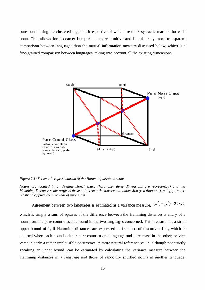
Figure 2.1: Schematic representation of the Hamming distance scale.

Nouns are located in an N-dimensional space (here only three dimensions are represented) and theHamming Distance scale projects these points onto the mass/count dimension (red diagonal), going from thebit string of pure count to that of pure mass.

Agreement between two languages is estimated as a variance measure, ⟨x2⟩+⟨ y2

⟩−2 ⟨ xy ⟩

which is simply a sum of squares of the difference between the Hamming distances x and y of a

noun from the pure count class, as found in the two languages concerned. This measure has a strict

upper bound of 1, if Hamming distances are expressed as fractions of discordant bits, which is

attained when each noun is either pure count in one language and pure mass in the other, or vice

versa; clearly a rather implausible occurrence. A more natural reference value, although not strictly

speaking an upper bound, can be estimated by calculating the variance measure between the

Hamming distances in a language and those of randomly shuffled nouns in another language,

15

⟨x2⟩+⟨ y2

⟩−2 ⟨x ⟩ ⟨ y ⟩ . The random shuffling simulates the case of a total absence of any relation

between the position of the nouns along the main mass/count dimension in the two languages, while

respecting the distribution of Hamming distances in each. Thus by comparing the actual value with

the reference value, we can get an understanding of how the languages match each other in broadly

classifying nouns on the main mass/count dimension. Each language however has different number

of questions analyzing its mass/count structure and hence the Hamming distance space for a

language is populated only at intervals of 1/Nth of a bit, where N is the number of questions in a

language. To minimize the effect of different intervals we estimate a true minimum of variance

between languages (which in an ideal case is 0) by calculating the variance between two languages

when all the nouns are ordered in the same way in their position on the Hamming distance scale. We

adjust the raw variance by simply subtracting the minimum variance for that pair, and then

normalize it by dividing it by the (adjusted) effective maximum value as mentioned above.

B) Clustering and Information Measures:

Information theory provides us with useful tools to quantify aspects of the clustering observed in

the data. The entropy of a variable, which can take a certain set of values, quantifies the uncertainty

in predicting the value it can take in terms of its possible values and their probabilities. A variable

which always takes a single value is perfectly predictable and has an entropy of 0 bits. A binary

variable has an entropy of 1 bit when it has 50% probability to take either value, e.g. 1 or 0. We can

apply this measure to the grouping structure formed around the mass/count distinction in the

languages we study. In our case, the variable G is which group any given noun or concept has been

associated to in a particular table, taking values 1,…,i,…,n, where n is the total number of groups

observed in that table. The probability p(i) is determined for our purposes as the relative frequency

of nouns/concepts assigned to group i. The entropy of the table is then calculated as:

H (G)=−∑i=1

n

p (i) log2 p (i)

16

H(G) informs us about the overall syntactic variability expressed (by an informant) in a language,

and can be regarded as the logarithm of an equivalent number of significant syntactic classes.

To make cross lingual comparisons, we quantify the extent to which the groups formed by

informants in one language overlap with the groups formed by those in another. This amounts to

defining equivalence classes, whereby two nouns are grouped together if and only if they are

members of the same syntactic usage group in the two languages. For example, if the nouns water

and wine are a part of the same group in language X and also fall in one group in language Y,

whatever the syntactic usage questions that define groups in the two languages, they are members

of the same equivalence class. For analyzing syntactic-semantic relations, language Y is replaced by

the semantic table. To give a limiting case, if two languages were to behave exactly the same in

classifying nouns in the mass/ count domain, the equivalence classes would coincide with the

groups formed in the individual languages, reflecting the exact match between groups produced by

language X and Y. At the other extreme, if two languages were to share no commonality, there

would be no relation whatsoever between the groups in the two languages, and membership in a

group in one language would not be informative about membership in the other language.

The mass/count similarity between X and Y can be quantified by the mutual information

I(X;Y), a measure that quantifies the mutual dependence of two variables. If two variables share no

common information then the mutual information between them is 0, which is the lower bound for

I, whereas the upper bound on mutual information is the lower between the entropies of the two

variables (the shared information between two variables cannot be more than the total information

content in one variable, i.e. its entropy). Mutual information is calculated using the joint entropy of

the two variables in question, which in our case is the entropy of the groups, by the relation

I ( X;Y )=H ( X )+H (Y )−H ( X,Y )

which can be written also

17

I (X ;Y )=∑ p (i , j) log2(p(i , j)

p(i ) p ( j))

and where H(X,Y) is the joint entropy of the two variables, at least equal to the higher of the two

individual entropies. In the limit case in which the syntactic groups are identical,

H(X)=H(Y)=H(X,Y)=I(X;Y), whereas in the opposite limit case, in which there is no relation

whatsoever between the groups each table, p(i,j)=p(i)p(j), expressing independent assignments, and

then H(X,Y)=H(X)+H(Y), so that I(X;Y)=0.

Mutual information measures suffer from a bias due to limited sampling [Panzeri & Treves

1996] related to the number of equivalence classes actually occupied compared to the total possible

(2Nq1 × 2Nq2) classes, where Nq1 and Nq2 are the number of questions for the two languages in

the pair. The correction to mutual information is estimated by calculating the mutual information

between the pairs of languages when the nouns for one pair are randomly shuffled, thus simulating

the lack of correlation between the two languages, and then averaging the value over 50 such

shuffles. The correction is then subtracted from the raw value calculated for a pair.

C) Artificial Syntactic String Generation:

To test the importance of the mass/count dimension and its link with semantics, an artificial

syntactic usage table was also generated, wherein the ‘yes/no’ decision to a syntactic question was

decided by a stochastic algorithm based on the position of the noun on the main semantic

mass/count dimension. This algorithm generates a 0 or 1 for each of a string of N ’pseudo-syntactic’

questions, one string per language, where N is the number of syntactic questions in that language.

To do so, it uses two reference points, namely the syntactic pure count string for that language and

the position of the noun concept along the semantic mass/count dimension, which is taken to be a

language universal. The latter is quantified by the Hamming distance from the pure count semantic

string, i.e. by the fraction d=D/N of semantic features that differ, for that concept, from those of the

pure count. Each bit of the artificial string is then assigned, one by one, for a given noun, the value

the bit has in the pure count string with probability (1–d), and the other value with probability d.

18

Syntactic questions, for this purpose, are empty of content, and simply refer to distinct bits

of a pseudo-syntactic usage string. Such bits are determined, for a particular language, by the

specific configuration of the pure count string for that language. If the noun is semantically close to

a pure count then the probability to generate a syntactic pure count, or something close to it, is

higher. The Hamming distances of the artificial strings from the pure count string have a certain

distribution (a convolution with exponentials of the semantic Hamming distance distribution) which

resembles that of the real syntactic strings, in most cases (except for Marathi, see below); while the

position of each noun along the artificial syntactic mass/count dimension is strongly correlated with

the position of the noun along the semantic mass/count dimension. The variance measure between

the pseudo-usage table of any language and the semantics table provides us with a lower reference

value for the variance itself, in contrast to the upper reference value obtained by random shuffling

of the nouns. We are then able to better gauge the significance of the mass/count dimension and the

importance of semantics with respect to the mass/count syntax. Also, the mutual information

between natural usage tables and semantics can be compared to the mutual information between the

pseudo-usage table and semantics, to allow a better estimate of what is the contribution of sheer

semantics to the mass count syntax (by providing what for the mutual information scale is a more

realistic upper value, see Fig. 12 below). The entropy for a particular language depends also on the

number of questions used to investigate the mass/count syntax. By looking at the entropies of the

artificial syntax we can see how the entropy measure scales with the number of questions.

2.2.3. Corpus Study of the Mass/Count Distinction in English:

Brown’s section of the CHILDES corpus was also used, in an additional component of the study, to

obtain mass/count information about nouns occurring in a natural English language corpus. For this

purpose all nouns were collected, in the adult-produced sentences of the corpus, which co-occurred

with a set of predefined mass/count markers. The co-occurrence frequency of a noun and the set of

mass/count markers was recorded and normalized to the total occurrence frequency of the noun.

Thus, for each noun, there was a set of numbers which indicated the statistical distribution of

syntactic markers for that noun. The markers that were used to measure co-occurrence frequency

were a(n), every/each, pluralization, many, much, some + sing. N, and a lot of + sing. N. This study

19

contains a total of 1,506,629 word tokens and 27,304 word types.

The usage table obtained from the CHILDES corpus was analyzed with multi-dimensional

scaling, and the distribution of the nouns on the mass count dimension. Multi-dimensional scaling

projects high dimensional data on a lower dimensional space while preserving the inter-data-point

distance, allowing to visually identify structural information in the data. By analyzing the

distribution and clusters in the projected space one can gain information about statistically

important dimensions and markers. Moreover, the data from the CHILDES cor-pus was analyzed in

terms of distribution of distances from the pure count class and of entropy measures, after

binarising the table indicating the frequency of each marker. Thus, for example, if a noun was found

at least once in plural form, this was taken as evidence that it could be pluralized; if found at least

once with a or an, that it could take the indefinite article, and so on. In this way, the same analyses

could be applied as for our database.

20

2.3. Results:

2.3.1. Individual Syntactic Rules and Semantic Attributes Do Not Match:

The starting point of our analysis is the observation that, at least in five out of the six languages we

considered, roughly half the nouns in the sample can be easily classified as pure count nouns. The

exact numbers in each language are Armenian: 1058, English: 693, Hebrew: 757, Hindi: 994,

Italian: 863, and Marathi: 255. For example, in both Italian and English nouns like 'act', 'animal',

'box', 'country' (as the territory of a nation), 'house', 'meeting', 'person', 'shop', 'tribe', 'wave'; and

'accident', 'cell' (as in biology), 'loan', 'option', 'pile', 'question', 'rug', 'saint', 'survey', 'zoo' were

classified as count in all respects by our informants. In Marathi, while the first 10 examples were

also classified as count, the second 10 tested positive on all count properties except one, usually the

property of having a morphologically distinct plural form. Marathi appears to stand out from the

group in other ways, as reported below. For all other languages, clearly the focus has to be on the

remaining proportion of non-pure-count nouns. (see appendix A6, A7 for details about each

question)

Among the informant responses, we observed cases of nouns that were regarded as pure

count in English but cannot be normally used with numerals in Italian ('back', 'forum', 'grin'), or

vice versa that test as pure counts in Italian but cannot be normally used with numerals in English

(such as 'behavior' or 'disgrace') Interestingly, when considering only usage with numerals and with

distributive each/every (ogni in Italian), our informants classified as ‘count’ in English nouns the

translation of which failed both tests in Italian: 'love', 'noon', 'youth' have count usages in English,

but not in Italian. The converse is also found: there are count nouns in Italian that, translated into

English, failed both the numerals test and the test “can be used with each/every”: 'advice', 'blame',

'literature', 'trust', 'wood'. There were cases where the impression of one of the authors was that his

or her judgment might differ from the informants, or the informants disagreed among themselves.

Since we are interested in this study in an overall quantitative analysis of cross-linguistic usage

judgments, we did not subject these differences of judgments to in-depth linguistic analysis, but

21

entered the judgments of the majority. We note that there were a significant number of such cases.

Overall, there were only 116 nouns that were classified as pure count in all six languages, and still

only 392 when excluding Marathi. We thus proceeded to a quantitative analysis, without further

questioning the responses by the informants on a noun-by-noun basis.

For a quantitative analysis, we first assessed whether, in any of the languages in the

database, a particular syntactic usage rule can be taken to reflect in a straightforward manner a

particular semantic attribute of the noun. While in many cases the yes/no answer to a syntactic

question turns out to be significantly or highly significantly correlated with a specific semantic

attribute, we found no cases where the correspondence could be described as expressing a ‘rule’,

even a rule with a few exceptions. To present quantitative results, we focused on cases where the

semantic-syntactic correspondence was higher. The notion of high correspondence is somewhat

arbitrary, because for example, one may contrast a case where among 10% of nouns with a

particular semantic attribute, 90% admit a certain syntactic construct, with another case where those

proportions are 30% and 70%. In our sample, the first ‘quasi-rule’ appears stricter, but it applies to

only 129 nouns in the sample, whereas the second one, while laxer, applies to 301 nouns. For

consistency with later analyses, we focus on relative (normalized) mutual information as a measure

of correspondence, while reporting also the number of nouns for which syntax matches semantics.

The relative mutual information measure ranges from 0 to 1 and it quantifies the degree to which

the variability in the syntax, across nouns, reproduces that in the semantic attributes, both of which

are quantified by entropy measures.

22

Language ++ +– –+ –– H(Lang) H(Sem) MI(S,L) Norm MI

Armenian 24 31 686 43 0.451 0.366 0.080 0.218

Italian 26 29 662 67 0.536 0.366 0.053 0.145

Marathi 25 30 559 170 0.819 0.366 0.020 0.054

English 29 26 668 61 0.503 0.366 0.046 0.126

Hebrew 29 26 682 47 0.447 0.366 0.055 0.150

Hindi 28 27 686 43 0.434 0.366 0.062 0.170

Table 2.4: A case of relatively high correspondence between a semantic attribute and a syntactic rule.

Semantic question 8, applied only to 784 concrete nouns, asked whether the noun denotes an entity (orindividual quantity) that can be mixed with itself without changing properties. (This somewhat looselyphrased question makes reference to the homogeneity and cumulativity properties discussed in section 2.1,since it can be interpreted either as asking whether proper parts can be permuted without changing thenature of the object, or whether instantiations can be collected under the same description.) The syntacticquestion considered was whether the noun can be used with numerals, and it was present in all languages.The largest group of concrete nouns, in the –+ class, denote objects that are not homogeneous, and thenouns can be used with numerals. The relative proportion of nouns in each of the four classes, however, yieldmeager normalized information values, indicating that individual attributes are insufficient to inform correctusage of specific rules, even in this ‘best case’ example.

Table 2.4 shows that most concrete nouns in our database (729/784) denote entities that,

according to our informants, cannot be ‘mixed’ while retaining their properties as instantiations of

the noun. Most of these nouns can be counted in the sense that they can be preceded with numerals,

across languages (with a somewhat less disproportionate bias in Marathi). Nevertheless, among the

nouns for which the answer to question 8 was positive, i.e. that displayed properties of either

cumulativity or homogeneity, roughly half can be used with numerals, again across languages,

yielding rather low values of mutual information between semantics and syntax, as quantified in the

last column of the table. Normalized MI (as mentioned in section 2.2.2 B) values are much closer to

zero than to one.

23

Even though the correspondence with the particular semantic attribute of cumulativity is

low, the results above suggest that there might be a high degree of correspondence among the

syntactic usage with numerals across languages, at least when excluding Marathi. After all, across

languages it is roughly half the nouns denoting entities which intuitively are cumulative, which can

be used with numerals, and half which cannot. Is it roughly the same half?

Language

pair++ +– –+ –– H1 H2 I(1:2)

Norm.

MI

Arm–Ita 662 48 26 48 0.451 0.536 0.124 0.275

Arm–Mar 560 150 24 50 0.451 0.819 0.059 0.131

Arm–Eng 666 44 31 43 0.451 0.503 0.106 0.235

Arm–Heb 675 35 36 38 0.451 0.447 0.095 0.212

Arm–Hin 683 27 31 43 0.451 0.434 0.129 0.297

Ita–Mar 548 140 36 60 0.536 0.819 0.062 0.115

Ita–Eng 654 34 43 53 0.536 0.503 0.131 0.261

Ita–Heb 652 36 59 37 0.536 0.447 0.068 0.152

Ita–Hin 661 27 53 43 0.536 0.434 0.102 0.235

Mar–Eng 547 37 150 50 0.819 0.503 0.041 0.082

Mar–Heb 553 31 158 42 0.819 0.447 0.034 0.076

Mar–Hin 556 28 158 42 0.819 0.434 0.037 0.086

Eng–Heb 669 28 42 45 0.503 0.447 0.119 0.266

Eng–Hin 675 22 39 48 0.503 0.434 0.144 0.331

Heb–Hin 675 36 39 34 0.447 0.434 0.078 0.181

Table 2.5: The correspondence between languages is not higher.

In the same case of relatively high correspondence between a semantic attribute and asyntactic rule, entropy and mutual information between languages yield the relatively lownormalized MI values listed in the fifth column, which indicate that a broadly applicablesyntactic question (“Can the noun be used preceded by a numeral?”) selects differentsubsets of nouns across different languages.

24

Figure 2.2: Agreement across languages remains low, however it is measured.

The solid bars show the normalized mutual information between pairs of languages for a single question, onusage with numerals, for concrete nouns only. The stippled bars are for the same measure over all nouns inthe database, both concrete and abstract. The patterned bars are for pairs of questions, on both the use ofnumerals and that of distributive quantifiers such as each/every in English (see text).

Table 2.5 and Figure 2.2 show that the naïve expectation is not met by the data. The

syntactic correspondence in the usability with numerals is weak across languages, even irrespective

of any semantic attribute it may originate from. The congruence (number of concrete nouns in the

same syntactic class when translated across languages) appears relatively high, because most nouns

can be used with numerals anyway, but, properly quantified in terms of normalized mutual

information, the degree of correspondence even excluding the special case of Marathi is roughly in

the 15–30% range, with English and Hindi reaching a peak value of 33%. When considering all

nouns in the database, including abstract nouns, the degree of correspondence does not change

much (stippled bars in Fig. 2.2). Again excluding the special case of Marathi, it falls roughly in the

20–27% range, with English and Hindi reaching a peak value of 39%.

One may ask whether the low MI values with semantics, in Table 2.4 above, may be due to

the lack of exact match between the semantic attribute considered and the specific syntactic rule.

Similarly, one may ask whether the weak correspondence in the pattern of usage with numerals may

also be due to the fact that numerals might point in different directions, so to speak, in the syntactic

space of each distinct language, for example, atomicity vs. non-homogeneity. To approach these

25

Arm-ItaArm-Mar

Arm-EngArm-Heb

Arm-HinIta-Mar

Ita-EngIta-Heb

Ita-HinMar-Eng

Mar-HebMar-Hin

Eng-HebEng-Hin

Heb-Hin

0.0

0.1

0.2

0.3

0.4

0.5

0.6

0.7

0.8

0.9

1.0

Normalised MI between languages pairs

1 Question: Numerals (Concrete nouns)

1 Question: Numerals (All Nouns)

2 Questions: Numerals and ‘every/each’ (All Nouns)

No

rma

lise

d M

I

issues, we have begun by considering pairs of attributes, and pairs of syntactic rules. The degree of

correspondence of each language with semantics does not change much, and in fact it tends to

slightly decrease. For example, when asking whether the object denoted by the noun can flow

freely, and also whether it is cumulative, and on the other hand whether the noun can be used with

numerals and whether it can be used with distributive quantifiers like ‘each’ in English, we find that

the normalized MI decreases with respect to the above analysis with one attribute and one rule, in

all cases except for Marathi (data not shown). The decrease is entirely due to the increase in the

entropy that appears in the denominator of the normalization (see Methods). In terms on non-

normalized mutual information, instead, adding dimensions reveals perforce more variability.

Similarly, the match between languages, independently of semantic attributes, does not

increase when considering two syntactic rules instead of one. Table 2.6 and Figure 2.2 report the

data, this time for concrete and abstract nouns together, when considering the two syntactic rules

above.

Table 2.6 shows that normalized mutual information values are low, all below 0.23 except

for the English–Hindi match, even though ‘congruence’ values appear high. Congruence is the sum

of the number of nouns that are used in the same way in both languages, with respect to the two

syntactic constructs considered. Except for pairs including Marathi, between 70–81% of nouns are

congruent across pairs. Yet mutual information is low because many of the congruent nouns are

simply pure count nouns in either language, accepting both numerals and distributives, and their

permanence in the largest class is not very informative about mass/count syntax in the other classes.

As considering two questions rather than one does not affect results, it is interesting to ask what

happens when considering all available questions together. We first focus on the main mass count

dimension.

26

Language pair H1 H2 I(1:2)

Norm.

MI Congruency

Arm–Ita 0.862 1.129 0.186 0.215 1119

Arm–Mar 0.862 1.427 0.109 0.127 825

Arm–Eng 0.862 0.872 0.176 0.204 1154

Arm–Heb 0.862 0.940 0.143 0.166 1152

Arm–Hin 0.862 1.242 0.172 0.200 1046

Ita–Mar 1.129 1.427 0.106 0.094 849

Ita–Eng 1.129 0.872 0.199 0.228 1132

Ita–Heb 1.129 0.940 0.141 0.150 1081

Ita–Hin 1.129 1.242 0.182 0.161 1011

Mar–Eng 1.427 0.872 0.094 0.108 882

Mar–Heb 1.427 0.940 0.082 0.087 826

Mar–Hin 1.427 1.242 0.122 0.098 812

Eng–Heb 0.872 0.940 0.191 0.219 1157

Eng–Hin 0.872 1.242 0.320 0.367 1099

Heb–Hin 0.940 1.242 0.169 0.179 1037

Table 2.6: Congruency and mutual information between languages.

The correspondence between languages is not higher when considering pairs of rules at a

time. Here we considered whether a noun can be used with numerals, and whether it can be used

with a distributive quantifier such as each/every in English.

27

2.3.2. Hamming Distance:

Plotting the data on the main mass/count dimension (Fig. 2.3) as the distance from the pure

count string shows that a very high proportion of the nouns are at a distance zero from the pure

count class (groups are labeled from 1 to N+1 at an increasing Hamming distance of a single bit,

where N is the number of questions and group 1 represents pure count nouns). Overall there is an

exponential-like decreasing trend in the group frequencies (see Appendix A9), as we go further

from the pure count, for all languages but Marathi. Since this measure does not distinguish between

different classes that are at the same distance from the pure count class but vary in the questions that

define them, we use different colors in the bars to show the proportions of particular classes at that

specific distance from the pure count class. The number of questions, N, is 9 for Armenian, 8 for

Italian, 5 for Marathi, 11 for English, 9 for Hebrew, and 5 for Hindi. Since there are N+1 possible

groups, we see that for Italian the 9th group is empty, whereas for Hebrew the last two groups are

empty.

Distributions in Figure 2.3 seem to reflect the nature of the nouns as brought out by the

questions used to investigate them. In the case of Marathi, the distribution is seen to have two

groups of high frequency, at the distance of 1 bit from the pure count class and mass class,

respectively. In each of these high frequency groups there is one class that accounts for most of the

nouns. The class making up most of 5th group differs from the pure mass class in answering ‘no’ to

the question regarding use of measure classifiers. Upon closer inspection, we find that, out of the

411 nouns that form the largest class in the 5th group, 332 are abstract nouns, hence answering ‘no’

to the measure classifier question. The question that differentiates, instead, the largest class in the

2nd group from the pure count class is ‘Pluralization with morphological change’, to which for

nouns in the largest class the answer is ‘no’. Figure 2.4 shows the same distribution, only for

Marathi, but restricted to the 650 abstract and to the 784 concrete nouns, respectively. Notice the

changes in the frequencies of the 5th group for both concrete and abstract nouns, as compared to

Figure 2.3. For other languages, the distributions restricted to concrete and to abstract nouns look

similar to the overall distribution, with a quasi-exponential downward trend (not shown).

In summary, the distribution of mass/count syntactic properties is undoubtedly graded rather

than binary, as might have been intuitively expected. Most common nouns are strictly count in

nature, in five of the six languages considered, with mass features increasingly rarer as they

approach the pure mass ideal. Marathi differs from the other languages, and it remains of be

28

examined whether it is representative of several other natural languages not considered in this study.

Figure 2.3: Distribution of nouns along the mass/count dimension. Each histogram reports the frequency ofnouns in the database, for a particular language, at increasing distances from pure count usage (1) andtowards pure mass usage (N+1), where N is the number of syntactic question for the language. Colors in thebars indicate the proportion of nouns in each of the syntactic classes occurring at the same Hammingdistance from the pure count.

Figure 2.4: The distribution for Marathi, restricted to concrete and to abstract nouns. As the 5th group in thehistogram in Figure 2.3 (top right) includes mostly abstract nouns, it dominates the abstract noundistribution (right), while it is considerably reduced for concrete nouns (left).

29

How distributed are the semantic features characterizing these same nouns? Figure 2.5

shows that, for concrete nouns, semantic features define a monotonically decreasing distribution

from the pure count class, roughly similar to that observed for syntactic usage features in five out of

six languages. Prima facie, this might suggest that concrete semantics might be the common source

that influences the global structure of the mass/count classification, at least for concrete nouns. For

abstract nouns, the two semantic questions considered leave most nouns in the ‘ambiguous group’

— in particular, in the class which includes abstract nouns without an easily definable conceptual

unit or a temporal unit. Since the semantics of abstract nouns does not have as clear a definition as

concrete nouns, it may not have a strong independent influence on the mass/ count syntax of

abstract nouns.

Figure 2.5: Distribution of nouns on the main mass/count dimension for semantics. Given the differentapplicable semantic questions, it is shown separately for concrete (left) and abstract nouns (right). Concretenouns show an exponential like shape similar to most of those in Figure 2.3, whereas most abstract nounsare in the ambiguous group.

If semantics serves as the common source of the mass/count syntax for concrete nouns, we

expect not only the distributions to look similar overall, but also to include individual nouns at

similar positions along the main mass/count dimension, both when comparing semantics with

syntax for each of the ‘well-behaved’ languages, and when comparing the syntax of two such

30

languages. This can be assessed through our variance measure, which quantifies the overall

difference between such positions.

Figure 2.6: Scatter plots of variance values along the main mass/count dimension. The adjusted andnormalized variance (see Methods) in the position of individual nouns is shown between semantics andsyntax (left) and between syntax in pairs of languages (right). In each plot, the adjusted and normalizedvariance for concrete nouns is on the y-axis and for abstract nouns on the x-axis. Pairs that include Marathiare indicated in red.

This expectation is only weakly borne out by the data. Figure 2.6 shows our relative

variance measure, which is normalized to range between zero (when individual nouns are

identically ordered in terms of their distance from the pure count class, either in both of two

languages or between semantics and the syntax of one language) and one (when the relative orders

are completely unrelated to each other). For concrete nouns, Figure 2.6 (left) shows that relative

variance from semantics hovers around 0.5, halfway to complete lack of any relationship. For

abstract nouns, variance values from semantics are somewhat higher. Marathi is an outlier, with yet

higher variance from semantics, for abstract nouns. It appears therefore that the relationship to the

underlying semantics is not very strong, even when considered solely along the main mass/count

dimension.

31

Between languages, the adjusted variance is less than 40% of the adjusted maximum for all

the pairs except for those including Marathi, both for concrete and abstract nouns. Marathi is an

outlier, with higher variances from semantics (for concrete nouns) and from other languages.

Marathi has higher variance since it does not have the exponential-like distribution as the rest of the

languages. The variance values calculated over the entire database tend to be, for each pair of

languages, close to the average between the values calculated over concrete and over abstract

nouns, separately (not shown). The fact that between languages variance values are relatively low,

relative to those from semantics, may indicate that there is an overall agreement across languages in

classifying the nouns in the mass/count domain. This is shown only a gross level, however, along

the main mass/count dimension, since here we do not take into account the fine grained differences

between the classes at the same distance from the pure count class.

2.3.3. Mutual Information along the Main Mass/Count Dimension:

The results from the analysis of the variance can be verified by considering an alternative

measure of the correspondence in the classification, the mutual information. Along the main

mass/count dimension, the mutual information can be calculated, e.g. between two languages, by

grouping nouns at each Hamming distance from the pure count nouns, rather than each syntactically

defined class. The mutual information (Table 2.7) ranges between zero (when there is no

correspondence whatsoever in the groupings) and the minimum of the two entropy values, where

entropy is calculated also by putting together all nouns in a group, i.e., at the same Hamming

distance from pure count nouns.

32

Language Entropy

*Armenian 1.63

*Italian 1.96

*Marathi 2.15

English 2.66

Hebrew 2.11

Hindi 1.54

*Semantics (2.01)1.58 (C) 1.24 (A)

Table 2.7: Language–entropy relations. Entropy values along the main mass/count dimension in the sixlanguages, and for semantics. The * sign indicates an ‘average’ over five informants (three for Marathi),taken by assigning to each question and each noun the yes/no answer chosen by the majority. For semantics,the overall value (in parenthesis) has little significance, because concrete nouns are assigned to eightdistinct groups and abstract to only three, and combining them distributes the abstract nouns into the twoextreme concrete groups and one central group.

33

Figure 2.7 confirms, on the different quantitative scale of mutual information measures, the results

obtained with the analysis of variance. The normalized mutual information with semantics is quite

low, and lower for abstract than for concrete nouns, corresponding to higher variance values. It is at

its lowest, 0.016, for abstract nouns in Marathi, which had the highest variance values. Between

languages, mutual information is somewhat higher, and not markedly different between abstract and

concrete nouns.

To better appreciate the significance of the relatively high variance values we measured, and

of the relatively low MI values, we contrasted the values obtained between different languages with

those obtained ‘within’ languages, i.e. measuring the correspondence between different informants

of the same language. These data are available for five informants each for Armenian and Italian,

and three for Marathi, and also five for the semantics classification. They give thus rise to 10

informant pairs in three cases and three pairs for Marathi.

Figure 2.7: Scatter plots of mutual information values along the main mass/count dimension. Thenormalized mutual information (see Methods) between the groups of individual nouns is shown betweensemantics and syntax (left) and between the syntax of pairs of languages (right). In each plot, the normalizedmutual information for concrete nouns is on the y-axis and for abstract nouns on the x-axis. Pairs thatinclude Marathi are indicated in red.

34

Figure 2.8: Scatter plots comparing variance with mutual information values.

The normalized mutual information (along the main mass/count dimension) is shown on the x-axis with thecorresponding normalized variance value on the y-axis, for abstract nouns (left) on and for concrete nouns(right). Different colors denote data points between the syntax of pairs of languages (empty circles), betweenthe semantics and syntax (red), within language (green) for 10 Armenian, 10 Italian, and three Marathi datapoints, and within different semantics informants (10 light blue data points).

Figure 2.8 shows, first of all, that the MI measure and the Variance measure are broadly

equivalent. Their relation is (very roughly) Var ~ (1–MI)4. This occurs despite the different nature of

the two measures: the mutual information is not sensitive to distance along the mass/count

dimension, only to group membership, whereas variance has limited sensitivity to small differences

in the exact classification of each noun, as long as its position on the mass/count dimension does

not vary too much. Variance turns out to be a more informative measure with our data, which better

span its 0–1 range, but mutual information can be easily generalized beyond the main mass/count

dimension.

Second, the within language data show mostly more agreement (higher MI and lower Var)

than the between language data. Exceptions are due to one Armenian informant (yielding four data

35

points) and one Marathi informant (yielding two more data points) that differ sensibly in their

syntactic judgment from the rest. The ‘average’ data for both Armenian and Marathi, however, due

to the majority rule effectively disregards their peculiarities. Thus both measures overall indicate

more agreement between informants of the same language than between languages, although this is

very far from a clear cut all-or-none difference. Confronted with the requirement to answer yes or

no to a set of binary questions, speakers of the same language vary substantially in their responses.

Third, the informants who contributed the semantic classification show the least agreement,

particularly for abstract nouns. Even though there were just two questions to answer for abstract

nouns, the responses to those two questions are effectively random, with the variance between

informants close to its random reference value (in one case exceeding it), and the mutual

information close to zero. This suggests that while the semantic properties that should inform the

mass/count syntactic usage are already not that salient and self-evident for concrete nouns, they are

completely irrelevant for abstract nouns.

2.3.4. Mutual Information across the Complete Syntactic Classification:

Mutual information is however higher when all the dimensions are considered (Fig. 2.11),

even in relative terms, i.e. when taking into account that the entropy values are higher for the full

classification (Table 2.8). Entropy values, as discussed in the Methods section, inform us about the

logarithm of the equivalent number of significant classes found in the data. Table 2.8 shows that the

entropies of the languages are in the range of 2–4 bits, which indicates the presence of something

equivalent to 22–24 equipopulated classes of nouns (from slightly above 4 for Hindi to just below

16 for English). In a hypothetical case where there were just two significant classes of mass and

count the entropy would have been in the range of 1 bit, in fact even less if the count class were, as

it turns out to be in most cases, much more populated. This provides a quantitative estimate of the

variability that exists in the mass/count classification, which is much higher than may have been

intuitively expected.

36

Language Entropy

*Armenian 2.29

*Italian 3.02

*Marathi 2.71

English 3.92

Hebrew 3.40

Hindi 2.12

*Semantics (3.72)2.94 (C) 2.34 (A)

Table 2.8: Entropy values for the full classification in the 2.6 languages, and for semantics.

The * sign indicates an ‘average’ over five informants (three Marathi), taken by assigning to each questionand each noun the yes/no answer chosen by the majority.

Figure 2.9: The entropy scales up with the number of questions. Both when calculated for natural syntaxand for the artificial syntactic strings used as controls, entropy values turn out to be roughly proportional tothe logarithm of number of questions, hence to yield almost the same value, around 1, when divided by thatnumber.

37

It is important to note that the entropy and mutual information values obtained with our procedure

are influenced by the number of questions used for each language. The scale of the entropy of the

‘artificial syntax’ depends solely on the number of questions, and we can see from Figure 2.9 how

also the entropy values for natural syntax are strongly correlated with the logarithm of number of

questions. Dividing the entropy of natural syntax (Table 2.8) by the logarithm of the number of

question all the entropy values get together at around the 1 bit mark.

The limited agreement that there is, is somewhat stronger for concrete than for abstract

nouns except for the 10 within Italian pairs. Figure 2.10 indicates that this holds within languages,

between languages, and much more so when including semantics. As noted above in the case of

measures restricted to the main mass/count dimension, the semantic classification of abstract nouns

is so arbitrary that agreement among the five informants that filled the questionnaire is extremely

low, and the correspondence of their majority response with any natural syntax is also low.

Figure 2.10: Scatter plots of mutual information values for abstract and concrete nouns. The normalizedmutual information is shown for abstract nouns on the x-axis with the corresponding value for concretenouns on the y-axis. Different colors denote data points between the syntax of pairs of languages (emptycircles), between the semantics and syntax (red), within language (green) for 10 Armenian, 10 Italian, andthree Marathi data points, and within different semantics informants (10 light blue data points).

38

Figure 2.11: Scatter plots comparing mutual information on the MC dimension with total mutualinformation values.

The normalized mutual information along MC dimension is shown on the x-axis with the

corresponding normalized mutual information including all dimensions on the y-axis, for abstract

nouns (left) on and for concrete nouns (right). Different colors denote data points between the

syntax of pairs of languages (empty circles), between the semantics and syntax (red), within

language (green) for 10 Armenian, 10 Italian, and three Marathi data points, and within different

semantics informants (10 light blue data points).

From Figure 2.11 we see that relative mutual information, when all the dimensions are taken

together, is only slightly higher than when just the main mass/count dimension is considered, telling

us that most of the variability is present along the main MC dimension. Again, abstract nouns show

a larger variability between and within languages, and this difference is particularly strong within

semantics. The source of the variability is most likely to be the degrees of freedom left in the

syntactic or semantic classification task, applied to the abstract nouns. Even though the nouns and

their meanings were disambiguated with a reference sentence, informants were still free to frame

39

the sentences while deciding whether a particular marker can be used with a particular noun. Hence

part of the variability may come as a result of the somewhat arbitrary determination of the exact

meaning used by different informants when adapting their abstract cognitive categories to the

classification of nouns, or of individual differences in the manipulation of context (Raymond et al.

2011).

Figure 2.12: Mutual information between language pairs vs. artificially generated control values.

Normalized mutual information between language pairs (red solid) are in the 0.33–0.52 range, except forpairs including Marathi, for which they are around 0.2. These values can be contrasted with the highervalues obtained by generating a pseudo usage table, based solely on semantic properties (red empty), asexplained in Methods. A similar comparison is shown for the normalized mutual information but only on theMC dimension (blue-solid for real and blue empty for artificial).

Figure 2.12 tells us that there while relative values are higher than when computed only

along the main mass/count dimension (Fig. 2.7), still there is little agreement across languages even

on a finer scale, as the MI values are mostly less than half of the lower of the two entropies. Mutual

information is a strict measure, wherein a single bit difference will put a noun in a different

equivalence class and lower the mutual information. In contrast, however, artificial syntactic strings

produced from the semantic ones, with the stochastic procedure outlined in Methods, share around

50% mutual information, relative to the lower of their entropy values. Artificial syntactic strings

also ‘suffer’ from a sensitivity to single fluctuating bits, hence the contrast between their 50%

agreement and the 20–30% (roughly) agreement of the real syntax tells us that real agreement is

40

Arm-ItaArm-Mar

Arm-EngArm-Heb

Arm-HinIta-Mar

Ita-EngIta-Heb

Ita-HinMar-Eng

Mar-HebMar-Hin

Eng-HebEng-Hin

Heb-Hin

0.0

0.1

0.2

0.3

0.4

0.5

0.6

0.7

0.8

0.9

1.0

Comparison of Normalised MI (Total/MC) for Real and Artificial Concrete Nouns After Sampling Correction

Mutual Information (Total) Mutual Information Artificial (Total)

Mutual Information (MC) Mutual Information Artificial (MC)

genuinely low, and it is not all due to using a bizarre measure. The low mutual information of the

natural syntax suggests that there is considerable syntactic variability along different dimensions of

the syntactic domain, although most of the variability is already in the main mass/count dimension,

since when restricted along that dimension agreement is even lower (Fig. 2.11–2.12).

2.3.5. CHILDES Corpus Study:

With a method analogous to the Hamming distance measures, we analyze the Brown's

section of the CHILDES corpus (only for the adult sentences) on the main mass/count dimension.

We simply count the frequency of occurrence of a noun with mass markers out of the total

occurrence of the noun in the corpus. There are 1551 nouns in this study out of which 522 nouns

(151 are abstract and 371 concrete) are in common with the nouns used for the analyses above.

Figure 2.13 plots the distribution of all the nouns on this main mass/count dimension. In a similar

trend to Figure 2.3, we see the nouns to be distributed all across the spectrum from count to mass,

with an overall decreasing trend in frequency going from count to mass (except for the pure mass

class). Nouns with pure count usage are very many compared to the rest of the groups. We do find,

however, a higher number of pure mass nouns in the corpus, as compared to the English syntactic

data obtained from an informant.

41

Figure 2.13: Distribution of nouns from the CHILDES corpus on the main mass/count dimension.

Count occurrences of nouns are very frequent as compared to mass occurrences, with nouns lying along theentire spectrum.

A multi-dimensional analysis of the corpus data brings forward four markers as salient, two

count (‘a(n)’ and Pluralization) and two mass markers (bareness and ‘some + singular noun’).

Nouns mostly lie along the vertices connecting these four markers. Figure 2.14 shows the most

significant dimensions in terms of the co-occurrence frequencies found in the corpus, for example,

along the edge connecting the vertices ‘a(n)’ and ‘pluralization’, close to the ‘a(n)’ vertex there are

nouns that occur almost always with ‘a(n)’ but seldom in plural form, in the corpus, while close to

the ‘pluralization’ vertex there are nouns with the opposite occurrence, with the rest of the nouns

occurring in between these two extremes. All nouns along this edge are in any case classified as

pure count nouns, in the first bin of Figure 2.13. The density of nouns along the count edge is much

higher than along the ‘mass edge’ (defined by the properties of appearing in bare form, at one

vertex, and appearing with ’some’ + singular noun at the other vertex). These four markers have the

highest variance in their frequency of occurrence across the nouns in the corpus (Table 2.9).

42

0 10 20 30 40 50 60 70 80 90 1000

200

400

600

800

1000

1200

1400

Percent Occurrence as Mass Noun

Fre

qu

en

cy

bare a/an every/each many pluralization much some a lot of

0.0485 0.1556 0.0044 0.0015 0.1177 0.0034 0.0275 0.0010

Table 2.9: Variance of the markers in the CHILDES corpus.

The variance of the markers we used to classify nouns in the Brown’s section of the CHILDES corpus wascalculated across its 1551 nouns, and the four markers with highest variance were used, a posteriori, tocharacterize the three most significant dimensions of mass/count variability, as independently generated bymulti-dimensional scaling.

Finally, we contrast mass/count entropy values extracted from the corpus from those

measured from the informant responses. To obtain entropy estimates from the CHILDES corpus,

which can be used for the comparison, we first binarise the corpus co-occurrence frequency table,

such that if a marker was found at least once with a noun, it was assigned the value of 1, and 0

otherwise. With this method, the total entropy of the corpus data was calculated to be 3.75 bits, as

compared to the English informant entropy, which is 3.92. Since 522 nouns (151 abstract and 371

concrete) are common to the corpus and informant usage tables, we calculated the entropy on the

MC dimension for them, too.

Informant entropy for concrete nouns on MC dimension 2.16

Corpus entropy for concrete nouns on the MC dimension 1.37

Informant entropy for abstract nouns on MC dimension 2.46

Corpus entropy for abstract nouns on the MC dimension 1.35

Table 2.10: The entropy values for nouns in both the database and the CHILDES corpus.

The entropy of the corpus on the MC dimension is lower than that of informants, perhaps

due to the restricted contexts in which sentences can occur in a corpus, as opposed to the freedom of

43

choice to the informants. The normalized mutual information, including all dimensions, between

binarised corpus and informant data after sampling correction is 0.051 for concrete nouns and 0.001

for abstract nouns.

Figure 2.14: Visualization of the nouns in the Brown’s section of CHILDES corpus in three dimensions, frommulti-dimensional scaling.

2.4. Discussion:

This is to our knowledge the first wide scale examination of cross-linguistic variation in the

expression of the mass count distinction, which attempts to investigate the question of the degree to

44

which the distinction is driven by perceptual-semantic attributes. Previous discussions in terms of

data have stayed more or less at the level of the anecdotal. Our major contributions to the discussion

are to show that the relation between such universal perceptual-semantic attributes and syntactic

usage in specific languages is very weak; as is the relation between languages: There is a core group

of count nouns where semantic atomicity corresponds directly with count syntax, but beyond this

there is indeed widespread cross-linguistic variation in whether or not a concept is expressed via

count syntax. In our sample of 1,434 nouns, in the five languages excluding Marathi, approximately

50% were what we would call ‘robustly count’, however only 392 were robustly count cross

linguistically. We have little to say about core mass nouns, of which there were few or none in our

sample. This might conceivably be because of the way in which we chose our data base, rather than

because of the inherently lower number of mass nouns in the languages. We leave it to other studies

to identify a significant core group of mass nouns, cross-linguistically. However the frequency

distribution from the native speakers is similar to the corpus obtained distributions.

We have made a number of observations which are relevant to the discussion of the

mass/count distinction:

I. Semantic or ‘real world’ attributes do not lead in a straightforward manner to individual

syntactic rules in the mass/count domain, hence we have to probe a potential mapping, for

any given natural language, between semantic attributes and a constellation of multiple

syntactic rules. The obvious alternation i.e. atomic vs. homogeneous does not predict mass

vs. count morphosyntax. This provides solid statistical support for the theoretical discussion

in [Gillon 1992; Chierchia 1998; Rothstein 2010], and many others.

II. When probing this domain with multiple syntactic usage alternatives, the distribution of

1,434 frequently occurring nouns in six natural languages is typically very far from binary.

The largest single class of nouns in five of the six languages was the pure count prototype,

i.e. the nouns classed ‘count’ by all syntactic probes. The rest are distributed in a graded

fashion, with fewer and fewer nouns having more usage properties opposite to those of pure

count nouns. Out of the 1,434 nouns, on average 873 were ‘pure’ count in a single language,

range [693–1058], when excluding Marathi (where the figure was 255), but only 392 were

45

‘pure count’ in all other five (‘typical’) languages.

III. Outside of the pure count nouns, the correspondence between languages is weak, even when

considering a single matching usage marker in each of the five non-exceptional ‘typical’

languages in the sample. In other words, learning what is a pure count noun, in any of these

five languages, gave no significant clues as to the content of the pure count class in any of

the other languages, beyond the 392 nouns which were pure count in all languages.

IV. Marathi differs from the other ‘typical’ languages in having a substantial fraction of nouns

close to a pure mass prototype, particularly among abstract nouns, and a distribution closer

to bimodal.

V. The semantic attributes that may be at the origin of the syntactic usage properties are

distributed similarly, across concrete nouns, to the typical syntactic distribution, with most

concrete nouns having ‘count-like’ attributes, and gradually decreasing proportions showing

progressively more mass-like attributes (as seen from figures 2.3 and 2.5).

VI. Despite the overall similarity between distributions, of semantic attributes and of syntactic

usage properties (in all languages tested except Marathi) the correspondence in position

along the main mass/count dimensions between semantics and syntax is very weak, even for

concrete nouns. Quantitatively, in terms of variance it is midway between fully matching

and random, and in terms of mutual information it is close to random. The different range

reflects the non-linearity of the MI measure, but both measures point at the weakness of the

observed correlation.

VII. Similarly, the correspondence between languages is weak, whatever measure is used.

VIII. Taking into account the detailed attributes and syntactic rules, rather than only the

main mass/count dimension, the correspondence remains weak.

IX. There is considerable variability also among informants of the same language; part of which

may be due to the testing paradigm.

X. A similar distribution along the main mass/count dimension can be gauged from 1,551

nouns extracted from the adult section of the English-language CHILDES database, after a

different analysis, namely in terms of graded rather than binary syntactic usage frequencies.

46

The three main dimensions of syntactic variability of nouns in the CHILDES database

describe an asymmetrically loaded pyramid: most nouns are countable, and simply vary in

their plurality at each instance; many fewer nouns span the other two dimensions,

characterized by an increasing frequency of use in bare form, and of use with some+singular

form, both mass-like attributes.

First, we have provided solid empirical evidence that count syntax is not a direct reflection

of atomicity in the denotation. Our initial aim to quantify the correlation (which we had presumed

strong) between non-homogeneous nouns and count syntax could not reach beyond a core group of

392 nouns which pattern as pure count in all languages checked, excluding Marathi. This indicates a

weak correspondence between perceptual/semantic and grammatical or morphosyntactic properties.

Note that the 392 cross-linguistically count nouns included approximately 27% abstract nouns (284

concrete and 108 abstract), thus it is not even possible to argue that count syntax correlates directly

with concrete atomic entities. Beyond this group of 392 nouns, the low level of mutual information

between any two languages indicates language-specific grammaticalisation of the distinction. This

means that it is no longer possible to assume a general correlation between atomicity and count, and

homogeneity and non-count. A preliminary examination of the 284 items in the pure count group

which are concrete rather than abstract indicates a high number of [+animate] nouns, in particular

individuals of a certain profession (scientist, nurse, preacher, slave, spectator), nouns denoting

buildings with a particular function (library, bank, apothecary) and nouns denoting artifacts that

individuals stand in an one-to-one relation with (wallet, watch, handkerchief). All these predicates

are atomic in an absolute sense, since they come in inherently individuable units, but they also

frequently occur in contexts in which a particular instantiation of the predicate is perceptually

salient. Thus it is plausible to posit that atomicity may be a necessary condition of a non-abstract

noun being robustly count cross-linguistically. However, beyond this there are no straightforward

generalizations.

The fact that these 284 nouns constitute between a third and a half of the robustly count

nouns, in any particular language, indicate that beyond this weak generalization the

grammaticalization of the correlation between atomicity and count differs from language to

47

language. Furthermore, there are 108 abstract nouns in the pure count group, where the criteria for

atomicity are by definition not well defined (since ‘atomicity’ is usually taken to express non-

overlapping properties of matter). One can at this stage hypothesize potential criteria, for example,

individuation via events: nightmare, appointment, and crash are all robustly count and non-concrete

and atomic instantiations can be potentially be individuated via temporally located events. But this

requires a notion of event individuation, itself problematic (see, e.g., Parsons 1990) and even then,

leaves open the question of which event-types are ‘inherently atomic’ and which not. The

conclusion for the linguist is that exploration of the basis of the mass/count distinction must be

language particular, and will involve semantic features far beyond the homogeneous/atomic

distinction.

We can draw a second theoretical implication from our results. We have seen that, for each

language (again excluding Marathi), the approximately 50% of nouns which are not purely or

robustly count in almost all cases cannot be characterized as ‘pure mass’. These nouns are located at

varying distances from the pure count class, depending on how many non-count features they have.

This could be taken as support for the view that mass/count syntax is imposed on a neutral root, that

it is appropriate to talk of mass or count ‘usage’, and that essentially, noun roots are flexible and can

appear in either context. This is the view taken in [Borer 2005], who claims that ‘being a count

noun’ is an exoskeletal phenomenon, the result of count syntax being imposed on a neutral syntactic

root. Our data, however, show that approximately 50% of the nouns in each language do show a

consistent count pattern, and furthermore, as stressed above, beyond the first 392 nouns, the choice

of which nouns are used consistently as counts is specified within a language (subject to some

idiolectal variation) and not across languages. This suggests that count syntax is a lexical

specification, and that beyond a core group, it is specified independently for each language.

A third point is that our data reveals cross-linguistically (again excluding Marathi) a large

group of pure count nouns, and no comparable group of mass nouns. This may be taken to support

the widely accepted view [e.g., Chierchia 1998, Borer 2005; Rothstein 2010] that mass syntax is the

default case, and that count nouns are derived from mass nouns via some form of operation, which

results in their sharing common properties. The degree to which Marathi differs from the other

48

languages studied also forces us to realize that languages with a mass/count contrast may differ

quite radically in how they implement it, and that the division of languages into those which have a

count/mass distinction and those which do not tells us little about typological variation.

The overall conclusion is that the questions that linguists have been asking should be

reformulated: Instead of looking for a general semantic characterization of the mass/count

distinction which will explain the grammatical distribution cross-linguistically, linguists should be

looking for language-specific patterns or generalizations, indicating that in a particular language,

certain lexical classes are or are not grammaticalised as count. (For example, a cursory examination

of the data indicates that Marathi is very restricted in allowing count syntax for abstract nouns.) If

there are cross-linguistic generalizations, we might expect for them to have an implicational

structure in the sense of [Greenberg 1963], i.e. we could look for patterns of the form: If lexical

class C1 is pure count, then lexical class C2 is also pure count. But it is an open question whether

we would find them at any significant level. We should avoid classifying nouns as ‘count’, ‘mass’

or ‘flexible’. In particular, our data show that non-robustly count nouns are flexible in different

ways and to different degrees. What these ways and degrees are is still to be investigated.

If there is a general characterization of the mass/count distinction, then it probably is in

terms of how the denotations of count (or mass) predicates are represented in the language, rather

than in terms of any real-world feature. For example, [Rothstein 2010] suggests that count nouns

denote entities which are indexed for the context in which they count as atomic. This leaves place

for particular languages to rank features which contribute to contextual salience, or to give them

different weights, which might then influence patterns in classifying nouns as count. Features which

weigh heavily in their contribution to count syntax in all languages would result in the set of pure

count nouns cross-linguistically. In any case, the set of robust count nouns and the lack of a set of

robust mass nouns indicate that we are more likely to find a general semantic characterization of

count nouns than of mass nouns.

At a deeper epistemological level, not only is mass count syntax largely left undetermined

49

by semantic attributes, it is also mistaken to regard it as a binary or quasi-binary structure. The

distribution of syntactic usage properties is very far from bimodal in five out of the six languages

tested, in fact it has nothing to do with bimodality. One is led to think of this grammaticalisation as

a graded self-organization process, operating within languages and to some extent within individual

speakers, and driven only to a limited extent by universal attributes, and plausibly governed or at

least constrained by language specific principles. However, at this stage we cannot tell to what

degree the grammaticalisation is governed, beyond the universal semantic or perceptual principles

that we have attempted to quantify, by language-specific principles of different nature, such as

cultural factors, historical accidents, individual language acquisition history, even context

dependence within individual speakers. What is already clear, however, is that a domain of

grammar, that to the non-specialist may seem rather straightforward, in fact opens new vistas on the

character of what are improperly called language ‘rules’.

50

Appendix A

The following tables are the equivalent of Table 2.1, for languages other than English.

No. Syntactic Questions

1.Can the noun be used with ‘a(n)’?

( +’ ’ )անորոշ գոյական մի հոդ

2.Number distinction: Can the noun be used with plural form?

( )հոգնակի թիվ

3.Can it be used in combination with numerals?

( )համադրում թվականների հետ

4.In combination with classifiers or measure phrases that manipulate

number? ( )համադրում դասակարգիչների հետ

5.Can the noun be used with ‘every’/’each’?

( / )Ամեն յուրաքանչյուր

6. Can it be used with ‘(a) little’? ( )մի քիչ

7. Can it be used with ‘(a) few’? ( )մի քանի

8.In combination of ‘many’ + plural form of noun?

( + )շատ գոյականի հոգնակի թիվ

9.In combination of ‘much’ + singular form of noun?

( + )շատ գոյականի եզակի թիվ

Table A1: List of questions used in Armenian to compile the usage table.

51

No. Syntactic Questions

1. Can the noun appear in the singular?

2.Can the basic form appear with af (as in af yeled lo ‘ana, ‘not a single boy

answered’)?

3. Is there a plural form?

4. Can the plural form of the noun appear with a number?

5. Can the singular form of the noun appear after kol ‘every’?

6.Can the singular form appear with kzat, me’at, harbe (‘a little, a little, a

lot’)?

7. Can the noun appear with tipa (literally ‘a drop’)?

8. Can the noun appear with a classifier?

9. Is it possible to say 10 + the singular form of the noun?

Table A2: List of questions used in Hebrew to compile the usage table.

No. Syntactic Questions

1. Can it be used with ‘many’/‘few’?

2. Can it be pluralized?

3. Can it be used with ‘every’?

4. Can it be used with numerals?

5. Can it be used ‘with a lot of’?

Table A3: List of questions used in Hindi to compile the usage table.

52

No. Syntactic Questions

1. Can the noun be in singular form with the indefinite article (un/o/a)?

2. Can it appear (suitably pluralized) with a numeral (due, tre)?

3.Can the noun appear with at least one singular indeterminate quantifier

(molto/molta/un po' di)? Note: non molto should not be considered.

4. Can the singular form be preceded by indefinite quantifier qualche?

5. Can the singular form be preceded by exact quantifiers (chili di, litri di)?

6. Can the singular form be preceded by non molto (‘not much’)?

7. Can it have a plural form with a definite article (i, gli, le)?

8. Can the plural form be preceded by exact quantifiers (chili di, litri di)?

Table A4: List of questions used in Italian.

No. Syntactic Questions

1. Can it appear with a numeral?

2. Can it be used in combination with an exact quantifier (kilo, liter)?

3. Can it be used with the article ek (‘a’)?

4. Can it be pluralized?

5. Does the morphology change when pluralized?

Table A5: List of questions used in Marathi.

Note: The questions were posed to the informants in their respective languages, not in the English

translation.

53

A6: Fraction of 'yes' answers to the questions above.

A7: Correlation between question pairs.

54

Question No. Armenian Italian Marathi English Hebrew Hindi Semantics1 0.90 0.89 0.57 0.37 0.99 0.91 0.112 0.90 0.81 0.09 0.87 0.77 0.90 0.453 0.83 0.27 0.67 0.87 0.88 0.78 0.544 0.05 0.85 0.66 0.83 0.84 0.86 0.525 0.94 0.08 0.23 0.85 0.91 0.83 0.446 0.18 0.16 - 0.85 0.30 - 0.047 0.85 0.88 - 0.30 0.16 - 0.048 0.85 0.01 - 0.29 0.08 - 0.049 0.14 - - 0.34 0.05 - 0.4310 - - - 0.19 - - 0.1411 - - - 0.12 - - 0.2212 - - - - - - 0.41

55

A8: Subgroups at each hamming distance.

A9: Exponential fit of the MC dimension distributions

Fit: y=A '+a e−bx

56

Armenian Italian MarathiGroup # of Subgroups Mean Size Std # of Subgroups Mean Size Std # of Subgroups Mean Size Std

1 1 1058 0 1 863 0 1 269 02 7 8.7142857143 10.531132983 8 20.625 20.975751306 5 9 191.861408313 15 4 7.3775721907 19 7.8421052632 18.454939591 6 21 39.7664012294 17 3.5294117647 4.302871818 17 5.2352941176 5.4946498042 6 12 4.59347363115 13 3.0769230769 3.2522181779 19 3.5263157895 4.6111991819 5 1 177.12058046 9 2.1111111111 2.260776661 13 4 6.5064070986 1 40 07 14 3.7142857143 4.7137861873 5 8 9.0829510623 - - -8 9 4.2222222222 6.8698212818 3 3 3.4641016151 - - -9 4 7.75 7.5443135318 - - - - - -10 1 15 0 - - - - - -

English Hebrew HindiGroup # of Subgroups Mean Size Std # of Subgroups Mean Size Std # of Subgroups Mean Size Std

1 1 693 0 1 757 0 1 994 02 11 16.363636364 28.688927227 9 27.777777778 30.987004445 5 34.4 47.7943511313 19 3.5263157895 4.9929775246 19 8.3684210526 16.197429585 10 8.2 7.48034461484 21 3.1904761905 4.8230596888 19 3.85 4.6822734019 10 7.6 7.32120208715 12 8.4166666667 22.589049372 19 4.3684210526 5.4488584566 5 15.8 16.7839208776 17 4.5882352941 9.0488868344 12 5.3333333333 8.3047996345 1 31 07 21 2.8571428571 5.4155859728 9 4.2222222222 7.8386506775 - - -8 15 2.2 2.0071301474 5 1.2 0.4472135955 - - -9 16 2.4375 3.2035136959 - - - - - -10 12 5.1666666667 11.01101377 - - - - - -11 8 4.875 7.1999503967 - - - - - -12 1 15 0 - - - - - -

57

Chapter 3

Attempts of a competitive neural network to decipher the mass-count

information

3.1 Motivation and a brief summary:

3.1.1 Introduction:

In the previous chapters we looked at a detailed statistical investigation of the mass-count

distinction with regards to its syntactic-semantic features, in this chapter and the ones following, we

move our attention to the 'cognitive' aspects of language processing. Our aim is to study the

properties of associative neural networks as a mechanism to sub serve syntactic processing in the

brain. In the current chapter a competitive neural network is applied to the mass-count database to

look at the self organising of nouns and markers in the neural space while later chapters involve the

study of a recurrent associative network which attempts to model global cortical mechanisms in the

brain.

The question of how the brain acquires language can be posed in terms of its ability to

discover, from exposure to a corpus, the syntactic structure of a specific natural language and its

relation with universal semantics. This has been a subject of study and of intense debate for the past

few decades (Barner and Snedeker, 2005, Barner and Bale, 2009). Natural language acquisition

appears to presuppose certain cognitive abilities like rule recognition, generalisation and

compositionality. These high-level abstract concepts should be realized in the language domain and

in specific sub-domains by general-purpose neural processing machinery, since there is no evidence

for dedicated circuitry of a distinct type for each sub-domain nor, for that matter, for languages a

whole [Tomasello 2003; Ogrady 2007]. How can rule recognition and generalization be

implemented in standard, vanilla neural networks? To explore this issue, we focus our attention on a

sub-domain of syntax, namely the syntax of the mass-count distinction. Following up on the results

of statistical analysis of the mass-count distinction in 6 languages, with relation to its cross-

58

linguistic syntactic and semantic properties, we now aim to study the learnability of those syntactic

properties by a basic neural network model, with the distant goal of eventually understanding how

such processes might be implemented in the brain.

We briefly summarise some of our main findings. As many linguistics studies have pointed

out, a simplistic mapping between homogeneity and mass syntax and/or atomicity and count syntax

on the whole would imply that the expressions denoting the same real world objects would be count

or mass cross-linguistically. However, this is not the case seen in Kulkarni, Rothstein and Treves

2013, words with a similar interpretation may be associated with very different arrays of syntactic

properties cross-linguistically. A noun which is associated with a count array in one language may

not be associated with a count array in a different language. Furthermore, over a sample of 6

different languages we saw that there is no binary divide into mass/count nouns, but rather a

continuum with a small group of nouns which are count with respect to all properties, and then a

range of nouns which are more of less count depending on how many count properties they display.

This makes the mass-count distinction an interesting linguistic phenomenon to model with its rich

diversity and lack of simple intuitive correspondence between syntax-semantics. Acquisition of the

correct syntactic usage of the mass-count nouns, by a child learning to speak, however should be

brought about by the same neural mechanisms in the brain that bring out other cognitive functions.

Thus the same neural principles of associative learning, proposed several decades ago, based on

Hebbian plasticity of co-active neurons, should serve as a functional mechanism to acquire the

knowledge of mass and count. We explore here, to what degree a standard neural framework with

unsupervised learning, can be useful to gain knowledge of what is mass and count in a particular

language.

3.1.2 Network modelling:

Our goal in the current study is to assess the learnability of syntactic and semantic features

of the mass-count distinction using simple neural networks. Artificial neural networks have a long

history as a method for neurally plausible cognitive modelling [Hopfield 1982; Elman, J, 1991;

59

Nyamapfene A. 2009], and can be endowed with properties including feature extraction, memory

storage, pattern recognition, generalisation and fault tolerance. Understanding how humans might

acquire the capacity for handling syntax in a specific sub-domain might start from encoding

syntactic/semantic knowledge into a neural network, which self-organizes with a prescribed

learning algorithm to recode that information in a neurally plausible format. That way one may

draw parallels about governing principles in the brain that bring about the acquisition of syntax.

Taking cues from biological neurons, most artificial neural networks employ ‘Hebbian’ plasticity

rules, wherein the synaptic connection between two units is strengthened if they are activated nearly

simultaneously, thus leading to associative learning of the conjunction or sequence of activations.

(See chapter 4, section I, II for more on neural networks and learning rules). Here we consider a

competitive network, a simple self-organising network which through ‘unsupervised’ learning may

produce a useful form of recoding. A competitive network, under the right conditions, is able to

discover patterns and clusters in a stimulus space and to train itself to correctly identify and group

inputs that share a close resemblance to each other. A competitive network is particularly interesting

in our case since much of linguistic information during language acquisition is rather 'discovered'

than explicitly taught. Moreover, mass and count nouns have been shown to exhibit differential

evoked potential responses, both with a syntactic and with a semantic stimulus [Chiarelli V, 2011].

We aim to study the performance of a simple competitive network in view of understanding how

well can syntactic and semantic features of the nouns in our mass-count database be accommodated

within a single network, thus exploring if the network can indeed achieve some rule-recognition

that will allow it to successfully categorise nouns in the syntactic mass-count space.

3.2 The network:

A) Classification of nouns:

Our network consists of a single input and a single output layer. At the input layer each unit

represents a syntactic feature (‘numeral’, ‘a/an’ etc) in case of the syntactic network or a semantic

feature (‘fixed shape’, ‘fluidity’ etc) for the semantic network. We label the network as 'syntactic' or

'semantic' based on weather the network is classifying syntactic or semantic markers. The input

layer is binary, and for each noun given as input a given unit can be active (activation value 1) to

indicate that the feature can be attributed to the noun, or inactive (value 0) to indicate that it cannot.

60

Thus a single learning event for the network includes the application of a binary input string

containing the syntactic or semantic information pertaining to a single noun, activity propagation to

the output units, and modification of the synaptic weights according to the prescribed learning rule.

B) Classification of markers:

Similarly, instead of self-organizing an output representation of nouns, we explore the self-

organization of syntactic features (‘markers’). Rather than an input noun with the features as

components, we apply as input a single feature/marker, with the nouns as components, i.e. there are

a few very long input string instead of many short strings.

On the output side, the number of units is variable, determined by the simulation

requirements. Unlike the input units, outputs units are graded, taking continuous values in the range

of 0 to 1.A competition amongst the output units based upon their activation levels decides the final

output level of each unit.

Figure 3.1. Schematic diagram of the artificial neural network, showing an input layer where units arebinary strings containing syntactic/semantic information of nouns and an output layer where units competewith each other to produce graded firing rates based on connection weights and on competition.

61

We use a fully connected network, where each input unit j is connected to each output unit i

with a synapse whose connection strength is given by w ij . The training sequence is executed as

follows:

An input is presented to the network and the activation hi of each output unit i is calculated

as

hi=∑j=1

N

r ' j w ij

where N is the number of input units and r ' is the input vector. The w ij ’s are initially set at random

values, which randomly causes certain output units to have a higher activation and lower activation

in others.

The final output firing of each unit r , is decided after setting up the competition between

output units as

r i=e(

hi

T )

∑i

e(

hi

T )

Here T governs the strength of the competition, lowering T makes the competition stronger

and as T approaches 0 it becomes ‘winner take all’, a case where only the unit which wins has a

maximum firing rate while all other units are suppressed to be inactive; whereas the competition

becomes softer as T is raised higher, allowing more graded output firing rates. Firing rates are

automatically normalised in the range of 0 to 1 by this form of the output function (thus also

allowing a probabilistic interpretation of the firing rates of the units).

62

In the next step we adjust the weights w ij according to the Hebbian rule, taking into account the

input and output firing rates of the units obtained in the previous step. The learning rule here is

slightly modified from the standard Hebbian rule to incorporate normalisation of the weights during

learning in a biologically plausible way. Normalising weights is important since it prevents a small

fraction of connections becoming too strong and resulting in the same units winning the

competition each time. The weights are adjusted at each presentation of an input as

δw ij =kri (r j'−wij )

k in the above equation controls the learning rate, i.e the size of increments in the weights as new

input-output pairs are presented to the network. The change in weight is proportional to the input

and output firing rates, however the second terms restricts a monotonous increase in weights by

causing a decay proportional to the activity of the output unit and to its existing synaptic strength.

One training iteration includes presenting each noun in the list once and the above process is

repeated for the desired number of iterations.

We now move towards the results section where we apply the above mentioned

unsupervised cluster discovering process to the participant data in 6 languages and semantics.

63

3.3 Categorisation of markers:

As described in section 3.2 B, we present as input the syntactic markers used in the

classification of the nouns. Here an input vector is comprised of N units, where N is the number of

nouns (784 in case of concrete nouns and 650 in case of abstract nouns), for each of the syntactic

markers. Thus an input includes information on how that particular marker is used over all the

nouns. Each input vector is presented once in one iteration, for 100 such iterations, which is also

when the synaptic weight matrix is observed not to change with further iterations. We use 3 output

units, N out=3 , with T = 0.1 and k = 0.01 for all languages except, Marathi (T=0.1, k=0.001). After

obtaining the output firing rates for each input marker at the end of the iterations, we calculate the

correlogram, representing how correlated the output vectors are with each other, hence giving

information about marker categorization. We show the mean correlograms over 100 distinct

network simulations.

Figure 3.2. Correlograms for 784 concrete nouns in each of the 6 languages in our study. Dark blue regions

represent complete lack of correlation (orthogonal vectors) while dark red regions represent congruent

vectors.

64

The correlograms in Figure 3.2 allow us to visually identify markers that fall in the same

category, as self-organized in the output of the network. High levels of correlation between two

markers signify close proximity in the firing rates of the output units for that pair of markers, and

are represented by light shades. For concrete nouns in Armenian, markers like ‘a/an’, ‘plural’,

‘numeral’, ‘few’, ‘every’ and ‘many+plural’ have a correlation of 1, thus occupying the same

position in the output space of the network. These are markers that can be applied to count nouns

and not to mass nouns. Instead, the typical mass markers of ‘measure classifier’ form an

independent representation, whereas ‘little’ and ‘much’ share the same position in output space but

distant from the count markers. Italian, Marathi, English and Hebrew follow the same Armenian

line of grouping count markers together and having separate but nearby representation for mass

markers, distant from the count markers. Hindi is different, as 4 of the 5 markers that were chosen

appear to be ‘count’ in nature, but all show gradation within the broad count category.

Figure 3.3. Correlograms, same as in figure 3.2, but for 650 abstract nouns. Note that markers areordered in the same way as in figure 3.2.

65

Results are similar for abstract nouns except for Italian having fewer graded categorisation

than for concrete nouns (figure 3.3) while for Hebrew ‘little’ and ‘tipa’ are co-incident.

The competitive network can be similarly tested on semantic features based on what value

each feature assumes over all the nouns. As seen in figure 3.4, semantic features are neatly divided

into mass and count features. Count features like ‘single unit’, ‘boundary’, ‘stable shape’ and

‘degradation’ all have a correlation of 1 with each other and 0 with mass features like ‘free flow’,

‘container shape’ and ‘mixing’. While ‘free flow’ forms a separate representation, ‘container shape’

and ‘mixing’ have the same output activation.

Figure 3.4. Correlogram of semantic markers for concrete nouns.

66

3.4 Categorization of nouns:

Similar to the process in section 3.1, we now present nouns as input to the network and

visualize the activation of the output units. The input vector here consists of N units for each

noun, equaling the number of markers for a language, hence containing information on how the

noun is used over all the mass-count markers for that language. The parameters used are Nout=3

(the number of output neurons), T = 1, k = 0.01 and Iterations = 10 (except for Marathi, the

parameters were: T=0.1 and k = 0.01). Figure 3.5 shows the position of the nouns in the 3-D output

space, where each axis represents an output unit. Axes are selected such that x ,y and z, respectively,

represent units in descending order of variance over the values of output activation they span. The

colour of each point signifies where that noun (or cluster of nouns, since nouns classified as

identical are co-incident) lies on the MC dimension as defined by the Hamming distance from the

pure count string (see section 1.1 A). Red indicates a distance of 0, thus pure count, while yellow

indicates a distance of 1, representing a ‘mass noun’. (convergence of learning is shown in appendix

B2)

Nouns are seen to approximately fall along a single line for all languages (a predominantly

linear structure for English and Marathi), barring an outlier at 0 which represents inputs that are

inactive for a noun. Moreover we can see a gradient from red to yellow, which implies that nouns,

even though not completely faithful, to a great extent lie along a gradient from ‘count’ to ‘mass’.

We further visualise the distribution of nouns on this line, so as to assess the frequency of nouns in

each cluster. The axis with maximum variance is selected and a histogram of the number of nouns

in each cluster along this axis is plotted.

67

Figure 3.5. Position of 784 concrete nouns in the output space as defined by 3 output units in 6languages. The gray scale indicates the Hamming distance of the noun on the MC dimension, fromred = ‘pure count’ to yellow = ‘pure mass’.

Figure 3.6. Histogram of nouns in reference to figure 3.5, along the axis of maximum variance.

68

Looking at the histogram of the linear alignment of clusters in the output space, we find that

the cluster near the red end has the highest number of nouns, which is followed by smaller bars

towards the mass end. Marathi is different, in having a significant cluster towards the yellow mass

end too. Note that the axis of largest variance is inverted for Marathi with the count end on the

higher side of X, this is because winning units are randomly selected.

It is interesting to note that a dimensionally reduced, entropy preserving representation of

the mass-count nouns has a notional similarity to the concept of the MC dimension as in chapter 2 ,

figure 2.3. The MC dimension was introduced as a concept to better understand the mass-count

division in terms of the ‘pure count’ string, but a competitive network with the appropriate

parameters is able to bring about a roughly similar distribution without needing a prior ad-hoc

definition.

Below are shown the same plots as in figure 3.5 and 3.6 but for 650 abstract nouns. Differences are

seen in English : the group of clusters of red count nouns is more stretched in a separate direction,

essentially having two separate lines for mass (yellow) and count (red) nouns.; Histograms on the

dimension of maximum variance show a similar gradation from count to mass and the difference in

Marathi with two significant peaks at the count and mass ends each.

69

Figure 3.7. Position of 650 abstract nouns in the output space as defined by 3 output units in 6 languages.The gray scale indicates the Hamming distance of the noun on the MC dimension, from red = ‘pure count’ toyellow = ‘pure mass’.

Figure 3.8. Histogram of nouns in reference to figure 3.7, along the axis of maximum variance.

70

3.5 The syntax-semantics interaction:

As we saw from the information theoretical analysis, the syntax and semantics of the mass-

count distinction share only a weak direct link, in the core structure of the count class, chapter 2,

figure 2.11. Thus acquiring the complete set of syntactic classes from semantic classes is not

possible by any learning mechanism, due to a lack of a direct one-to-one correspondence. However

it is improbable that syntax and semantics are independently learned without any mutual interaction

during learning of mass-count concepts, and there is no evidence that either one is learnt before the

other [David Nicolas, 1996]. From the classification of markers above, we see that broad categories

of mass and count can indeed be extracted out of the data, interestingly for both syntax and

semantics, thus rendering some semantic sense to the syntactic distinction. Classes of nouns

however, formed from these markers do not reflect mass-count information in a straightforward

manner between syntax and semantics. Hypothesising an underlying commonality of the mass-

count divide between markers of syntax and semantics,we test the performance of the competitive

network when syntax and semantics are simultaneously part of the input space during the learning

phase, and test the correspondence between the syntactic and semantic classes after learning.

3.5.1 Quick summary of information measures:

We use mutual information as a measure to analyse the correspondence between two

representations, encoded either in a syntactic network trained on input information about marker

usage for the nouns in a particular language, or in a semantic network trained on information about

the semantic properties of the nouns. Here we focus on systems that have undergone a slow process

of self-organisation to categorise their inputs.

We first begin by calculating the entropy of the output of the network and the information it

contains about the clustering of nouns in the input. Nouns are clustered together if they have exactly

the same output firing rates. So in effect the output, labelled as O, contains n clusters 1... i ... n ,

71

where each cluster contains nouns that are classified as identical by the network. Entropy is then

defined as

H (O )=−∑i=1

n

p ( i ) log2 p (i )

Where p(i) is the ‘probability’ obtained as the relative frequency of the nouns in the cluster i .

To calculate mutual information between two representations X and Y we first obtain

equivalence classes, i.e. groups where a particular set of nouns has been clustered into the same

class in both X and Y. For example, if nouns like ‘man’ and ‘dog’ fall in the same cluster in X and

are also found in the same cluster in Y, they belong to the same equivalence class. The joint entropy

of X and Y, H (X ,Y ) is then used to calculate the mutual information a

I ( X;Y )=H ( X )+H (Y )−H ( X,Y )

Alternatively, one may consider a joint probability distribution table of nouns in X and Y

from the equivalence classes, and calculate mutual information as

I ( X;Y )=∑i,j

p ( i,j ) log2( p ( i,j )p (i ) p ( j ) )

Mutual information co-varies with the relevant individual entropies, so to facilitate

comparisons we use normalised mutual information. When X and Y show completely unrelated

clusters, p(i , j)=p (i) p ( j) the mutual information is 0, giving it a strict lower bound. It has a

natural upper bound in the sense that the mutual information between X and Y can never be greater

than the lower of the two entropies H (X ) ,H (Y ) . Thus for comparison purposes we define

72

normalised entropy as I(X ;Y )/min (H (X ) ,H (Y )) , which lies in the range of 0 to 1.

3.5.2 Processed Interacting Mutual Information:

First, to compare with previous results, we have calculated the baseline mutual information

between syntax and semantics by providing only semantic information to the network, with no

syntactic information during the learning phase. The mutual information was calculated between

syntactic data and the output of the semantic competitive network. When no syntactic information is

present at the inputs, the resulting mutual information is about equal to the mutual information

between the syntactic and semantic data calculated using the procedure in chapter 2, section 2.2.2-B

A) The effect of competition strength:

The competitive network brings about a dimensional reduction from a high dimensional

input space to a lower dimensional output space defined by the number of output units. Furthermore

the strength of the competition affects how different input clusters collapse onto each other,

depending on the distance between them. These processes reduce the entropy from its input value,

which critically affects the available mutual information between two data sets, when measured at

the output. We observed that the network failed to consistently learn when the number of output

units, N, was less than 3 and that there was no noticeable change in information measures for N ≥ 3.

Thus we set N =3 and varied the competition strength T to see the effect on the output entropy of

the network. Figure 3.9 plots the ratio of the output entropy to input entropy of the network for

various values of T. Since no information is added during processing, the output entropy is at most

equal to the input entropy or less otherwise.

73

Figure 3.9. Variation of the output entropy to input entropy ratio for different values of the competition

strength, T.

Figure 3.9 shows, at around T = 1, input and output entropies are comparable for all languages

(except Armenian at 1.5), and tends to drop on either side (especially for syntax), thus we select T

= 1 as optimal value of competition (when maximum information is retained after processing), to

calculate mutual information between syntax and semantics.

B) Combined learning of syntax and semantics:

Syntactic information is then provided to the network in a partial manner, in a proportion γ ,

which signifies the fraction of input units of the syntactic segment of the input string that are set to

the activation levels of the syntactic string of a particular language. γ=0 represents when none of

the syntactic input units are receiving any information and are set to 0; while γ=1 implies all of

74

the syntactic information is present; for in-between cases a fraction 1−γ units are randomly

selected and set to 0. Thus we can vary the amount of syntactic information available to the network

during learning and test the effect on the syntactic-semantic mutual information and weather the

relevant syntactic and semantic classes are brought together in any systematic way. We train and

test the network by providing the same proportion γ of syntactic inputs along with the semantic

ones.

Figure 3.10. Mean normalised mutual information over 10 independent simulations at various γ

values for concrete nouns in 6 languages when N=3 output units, and 10 iterations.

Figure 3.10 depicts the performance of the network when it is tested on the training set as

the semantic inputs are incrementally supplied with syntactic information. The green curves

represent the mutual information between unprocessed semantic and syntactic input, this is the

75

baseline mutual information between semantic and syntactic data which remains flat, i.e. roughly

independent of γ , the small variations on this flat line are due to the random selection of units that

receive syntactic information at each run. The red curves represent the mutual information between

the output of the network and unprocessed syntactic inputs while the blue curves plot the mutual

information between processed semantic and syntactic outputs. The dashed and dotted curves tend

to follow each other closely, implying that the syntactic competitive network results in a

dimensionally reduced faithful representation of the syntactic input data. The mutual information

rises above the baseline as γ increases above the 0.4-0.5 region for Armenian, English, Hebrew

and Hindi, and above the 0.2 region for Italian and Marathi. Thus semantic classes tend to gradually

realign, with increasing γ , in such a manner that they correspond more to the syntactic classes as

compared to the baseline. This reorganisation is however very limited: at γ=1 , the normalised

mutual information for all languages is in the range of 0.5-0.6, which is around half way towards

full agreement. Although interacting with syntax does help some reorganisation of the semantic

classes, the divide between syntax and semantics is clear and almost half of the semantic

information cannot be shared with syntax at γ=1 .

The performance of the network is further limited by the fact that it cannot be driven by

semantic units only, with no syntactic information during testing. A ‘syntactic context’ is necessary

at the inputs for the network to result in a mutual information performance above baseline. When

tested without syntactic information, or with only a partial amount, the drop in the normalised

mutual information is significant, with only a tiny trace of learning shown by the network.

3.6 Discussion:

. This is a first attempt at assessing the learnability of the mass-count statistical data and

rather an exploratory study towards a network modelling of the classification. By applying such a

network to the mass-count information from participants we can draw a few inferences:

76

1. In most languages, syntactic markers tend to categorize ‘spontaneously’ between

mass and count markers, lending validity to the intuitive perception of a quasi-binary

distinction. This is not fully true, however, and particularly in Hindi the markers

chosen show a graded distribution of mutual correlations. Hindi however is slightly

different from the remaining languages, in such that the 4 out of 5 markers in Hindi,

answer 'yes' for pure counts. Thus the network is driven towards a count-internal

categorisation.

2. Nouns, instead, tend in most languages to distribute quite closely along a line which

coincides with the main mass/count dimension introduced in our previous study

(Kulkarni, Rothstein and Treves, 2013). Along this line, nouns are very crowded at

the count end, and scattered all along towards the mass end. Their distribution is

therefore graded rather than binary, with no emergence of a single ‘mass’ class, but

rather of several non exclusive but distinct ways of a noun of being different from

pure count. For example, in Armenian (Figure 8) nouns like ‘bird’ and ‘ship’ belong

to the ‘pure count’ class while ‘troop ’and ‘lunch’ are in the 9th class away from the

count class. On the mass end, nouns like ‘cotton’ and ‘milk’ are at the extreme mass

end of the spectrum while ‘coffee’ and ‘wheat’ are more mass-like nouns but not at

the pure mass end. The exception is English, where there are at least two clear non-

equivalent dimensions of non-countability.

Both the above observations are interesting because the mass-count information in the

categorisation arises on its own. The markers, in some cases, very cleanly segregate themselves into

mass and count. The nouns are reduced to a one dimensional representation along a mass-count

spectrum. Even though the network fails to associate specific syntactic markers with specific nouns

based on the semantics, the network does develop a 'concept', if we may say, of what is the mass-

count classification. The diversity and richness of this classification however, prevents a simple

network to learn specific associations. Which brings us to the third observation,

77

3. The lack of significant mutual information between semantics and syntax implies, as

we have verified, that the latter cannot be extracted solely from the former. Further,

when allowing the competitive network to self-organize on the basis of full

semantics and partial syntactic inputs, and testing it with the full syntactic inputs, the

mutual information obtained with the full syntactic usage distribution is only at most

about half the corresponding entropy value. This occurs in fact only when the full

syntax is given in the input also at training, and it indicates that giving also

semantics information affects negatively rather than positively the performance of

the network.

Overall, these observations indicate that the acquisition of the mass-count syntax by humans

with neurally plausible mechanisms, involve more complex computations beyond what can be

captured by a simple neural network. The observations do however,reinforce the conclusions of

our earlier study that mass count syntax is far from a rigid binary rule, rather it appears as the

flexible, speaker-specific usage of a variety of binary markers to a quantitatively and

qualitatively graded repertoire of nouns, where being non-count can be expressed in many ways

(see also, chapter 2, figure 2.8 and 2.11). Taking semantics into account helps speakers to a very

limited extent in generating their own mass/count ‘dialect’.

78

Appendix B

B1: Log plots of figures 3.6 and 3.8

a) Concrete Nouns

b) Abstract Nouns

79

B2: Convergence of weight matrix during learning. (change in weight matrix against iterations)

a) Concrete Nouns

b) Abstract Nouns

80

B3: Correlation coefficients of groups in figures 3.6 and 3.8 with MC dimension groups in Chapter 2, section 2.

81

Concrete AbstractArmenian 0.865 0.833Italian 0.507 0.578Marthi 0.057 0.301English 0.718 0.498Hebrew 0.414 0.61Hindi 0.277 0.329

Part B

Storing Correlated Memories and the Possible Spin GlassNature of the Potts Neural Network

82

Chapter 4

Section I

The Potts Neural Network

A] Introduction:

In the previous chapter we have already seen the application of a neural network, namely the

competitive neural network. In this chapter we look at a more complex network, and at some of its

features in section II and III, which are particularly relevant to cognitive function including

language acquisition. Section I summarises the basic concepts of neural networks and some past

work in the field. First, let us have a quick recapitulation on neural networks.

Neural network models, to a great extent, are a product of the connectionism concept.

Connectionism is founded on the idea that the core information necessary for cognitive function is

stored in the neurons and in their synaptic connections in the brain. The connections are modifiable

and respond to the exposure to various inputs, bringing about a 'learning process' in the network.

One of the popular earlier models was the Parallel Distributed Processing model (PDP),

[McClelland, Rumelhart 1986]. It consisted of having several independent parallel processing units

called 'neurons' which were connected with a specific structure. Neurons were essentially variables

taking a certain range of values decided by an output function and the structure of connection

amongst them was given by a connectivity matrix of real numbers that represented the strength

between two units. Much of the modern work on neural networks follows the same fundamental

principles.

B) Types of neural networks:

Different classes of models can be defined from the structure of the connectivity and the

details of how the neuron is modelled. One may model the detail the time dependent voltage-current

response of a neuron [for eg. Izhikevich 2003], or use more abstract units which essentially only

83

represent the firing activity of the neuron [an eg. Hopfield 1982]. We use the latter, since we are

interested in the global behavior of a large number of interacting neurons, for which one can

approximate the behavior of a neuron with its mean firing rate [Gertsner 1992a; Gertsner 1992b]. A

synaptic connection between neurons is modelled by another variable J ij , between neuron i and j,

whose strength is changed according to Hebb's rule [Hebb 1949]: the change in connection strength,

δJ ij , in a learning event is proportional to both the pre and post synaptic activity of the two

neurons in the event. Some other learning mechanisms like the discriminative learning, especially in

the language domain [Bayen et al 2011] aim to achieve learning by the adjustment of conditional

probabilities between 'language objects'. However we restrict ourselves to biologically inspired

mechanisms like the Hebb's rule, rather than the powerful but maybe biologically implausible

machine learning rules. Or at least, if one wishes to manifest a similar model in biologically

inspired neurons, one must revert back to a Hebb like situation.

i) Different connectivity structures give rise to different types of neural networks. The very

first neural networks were of the feed-forward type [Hornik 1989]. It consists of an input layer and

an output layer which learns the association between 'representations' of inputs and outputs via

modifiable connections between the two layers. It was found that adding another 'hidden layer'

between the input and out layer, such type of network can potentially map any continuous input-

output function. However, multilayer feed-forward networks predominantly operate with the back-

propagation algorithm, in which the error between input and output travels backwards through the

connections to adjust each connection strength. The biological plausibility of this method is

unlikely. Since the network requires a training set of output patterns, this is a supervised learning

algorithm.

ii) Another class of neural networks is when there is no 'teacher'; this is called the unsupervised

network. We have seen an example of such a network in the previous chapter, one which uses

competition between the output neurons during learning and classifies the inputs. These are self-

organising networks which can form clusters and categorise inputs based on a similarity measure,

without the requirement of an explicit target output. One may suppose that unsupervised networks

84

form the first block of information processing where novel stimuli are categorised to be processed

further.

iii) A third class of neural networks are the recurrent neural nets [Amit 1989], where neural

activity is fed back to the same neurons by recurrent synaptic connections, thus forming a cycle of

information flow. [Elman 1990, 1991] constructed one such type of a recurrent net called the

'Simple Recurrent Network' (SRN) and applied it to linguistic stimuli. Elman’s SRN had a modular

structure and was a mixture of feed-forward and recurrent modules. His important finding was that

the SRN could segment a continuous unbroken stream of words from a sentence into separate words

that were clustered in grammatical categories of nouns and verbs.

Another class of recurrent nets is the autoassociatve network, where the inputs learn

associations with themselves and thus facilitate a content addressable memory. The stored

memories are attractors of the dynamics of the network and with a partial cue the network can can

recover the entire memory of the object, for example, giving a cue like 'to e_r _s h_m_n' may

recover the entire phrase 'to err is human'. Our model, to be discussed in Section C, falls into this

category. It is of special interest to us due to its powerful computational abilities, which may help to

replicate how some of the cognitive functions in our brains are brought about.

Figure A: A schematic representation

of an autoassocitive network with

recurrent connections. (reproduced

from [Rolls, Treves 1999])

[Hopfield 1982] designed such a network from the Ising model of interacting spins which

was mathematically treatable and hence led to an intense study, revealing the rich dynamics of such

85

models which can serve as the foundation of cognitive function. The neuron was abstracted to two

states of being active(+1) or inactive (-1) and N such neurons were connected by 'synapses', e.g.

synapse J ij between neuron i and j. The learning rule was prescribed in such a way that each

pattern, ξiμ , i=1,2. .. N ;μ=1,2. .. p , for N neurons and p memories to be stored, was situated at the

bottom of a valley on the energy landscape, thus forming an attractor. The energy is defined as

H=−12∑i , j≠i

N

J ijξiμ ξ j

μ

This term is called the energy because for a suitable definition of the dynamics, a symmetric

J, and in the absence of noise, a flipping of a spin will occur if either it keeps the energy of the

system the same or it reduces it. Hence over many such spin flips the network naturally reaches a

stable state which is the minimum of the energy function. The Potts model, which we study in

section II and III, is in a sense an extension of the Hopfield model where the fundamental unit is not

a model neuron and it is not restricted to the two states of an Ising spin, but it can be in more than

two possible states.

Figure B: Energy landscape depicting attractor dynamics.

86

C) The Potts neural network model for cortical dynamics:

The cortex is a large network of interconnected neurons and is thought to be composed of

several sub-networks with dense recurrent connectivity. These sub-networks are also interconnected

with each other, thus communicating information to and fro over the whole cortex. [review on

functional connectivity: van den Heuvel, Pol 2010, Yeo et al 2011 ]. The Potts neural network

model, the one described below, is an adaptation of the Potts network studied in [Kanter, 1988;

Bolle et al, 1993]. Our model aims to present a simplified model of cortical mechanisms with

adaptive dynamics. It is a global autoassociative network of interacting units, each unit representing

a local sub-network.

a) The Potts unit: The model we study is a variant of the Potts neural network model [Kanter

1988] aimed at incorporating the time dependant dynamics of cortical mechanisms in the global

attractor space [Treves 2005; Russo, Treves 2012]. A Potts unit, σik , represents the ith local cortical

patch which is in the local attractor state k. Each unit can be in S possible states, hence the internal

dynamics of the local patch are reduced to a simplified representation to depict only the local

attractor states. At a given time, a single unit might be correlated to only one of its attractor states or

partially correlated to more than one. With N such units we can represent a global pattern over the

entire cortex, ξi , k for i=1,2. ..N ;0⩽k⩽S . s=0 is defined to be the inactive state of the unit. The

total activity of a unit if fixed to 1, thus ∑l=0

S

σ il=1 . Several distinct combinations of states can

produce different patterns, ξi , kμ , where μ is the pattern identity, μ=1,2... p .

Figure C: Conceptual visualisation of the Potts model, with

local patches represented by S state interconnected units,

forming a global cortical network.

87

b) The connections: Local patches are connected with long range synapses which communicate

the activity of unit i in state k to unit j in state l by an interaction term J ijkl . J forms a

connectivity matrix which stores information of several patterns ξμ which are embedded in the

network by a learning rule [Russo, Treves 2012], which is similar to the one in the Hopfield

network but adapted to S-state units.

J ijkl =

c ij

Cm a(1− aS )∑μ=1

p

(δξiμk−

aS)(δξ j

μl−aS)×(1−δk0)(1−δl0)

c ij , is a binary number [0,1] which establishes the existence of a connection between unit i and j ,

c ij is randomly distributed across the connections and is 1 with probability Cm/N , with c ii=0 ,

where Cm is the number of connections between units. a denotes the sparsity of patterns, so in

effect a fraction Na units are active in a state 0<k⩽S . The term a/S reduces bias due to random

overlaps and is discussed in chapter 4, section II, 4.7.1. The last two product terms arise out of

biological reasoning and make sure that learning occurs only on active states and that the 0 state is

ineffective over J.

c) Adaptive Dynamics: Once the network has reached a stable attractor state, the active units

are continuously 'firing', but in a biologically realistic scenario the units cannot go on firing

continuously forever. Hence besides the constant baseline global threshold U , we introduce two

thresholds that account for neuronal fatigue and slow inhibition [Horn, Usher, 1989]. They deplete

the resources for the unit to fire and eventually destabilise the attractor. The first kind of threshold,

θik , which affects only active units, σi

k , intends to model neural fatigue and short term depression

88

[Tsodyks, Markram, 1997 ] and has a time constant, τ2 in the in order of tens of milliseconds. The

second threshold, θi0 , affects only the inactive state and models slow, delayed inhibition within a

cortical patch and has a time constant τ3 in the range of hundreds of milliseconds. The dynamics of

the thresholds can be stated in the following way,

τ2

dθik(t)

dt=σ i

k−θi

k ; τ3

d θi0(t )

dt=∑

k=1

S

σik−θi

0

A third time constant, τ1 , determines the rate of integration of the local fields over each unit,

subject to the dynamic threshold. The local field is the summed inputs that a unit receives from all

other units, given by hik=∑

j≠i

N

∑l=1

S

J ijklσ j

l+w (σi

k –1S∑l=1

S

σil) . The second term is an addition, that

models self-reinforcement in the local patch dynamics of an active unit, to make it converge

towards an attractor. Hence the final inputs that a unit receives can be written as

τ1

drik(t)

dt=h i

k(t)−θi

k(t)−r i

k(t)

with rik being the input to the active states and θi

0 to the inactive states. The final state of the unit

can be written as,

σik=

eβr i

k

∑l=1

S

eβ ri

l

+eβ(θi

0+U )σi

0=

eβ(θi

0+U )

∑l=1

S

eβ ri

l

+eβ(θi

0+U )

89

where β represents the local patch inverse temperature thus modelling noise internal to the unit

(more about this in chapter 4, section III, 4.13). The global dynamics of the network however, is

noiseless.

D) Latching behavior:

The above equations completely describe the dynamics of the Potts neural network model

with adaptive thresholds. The introduction of the adaptive thresholds generates some interesting and

potentially useful features in terms of cognitive aspects. As the network reaches a stable attractor

state, active units in the network start facing an increasing threshold, which destabilises them and

the network starts falling out of the attractor. However it may happen that as the network falls out of

the attractor it is pushed towards a new basin of attraction and enters into a new attractor. This

process may continue endlessly in the right parameter phase space. In fact the network shows three

phases of dynamical behaviour [Treves 2005; Russo, Treves 2012]: (a) No latching - the network

falls out of the attractor and it decays into inactivity; (b) Finite latching - the network falls out of an

attractor subsequently jumping into another one and this process continues for a finite duration; (c)

Infinite latching - the sequence of jumping continues indefinitely.

It was observed that the jump from one attractor to another is facilitated if the two attractors are

correlated.

90

Figure D: Latching behavior of the Potts network. (a) No latching; (b) Finite latching; (c) Infinite latching.(reproduced from Russo, Treves 2012)

E) Application of the Potts neural network to language:

The latching phenomenon in the Potts network and particularly the fact that latching

transitions are more probable amongst correlated patterns makes it a good model to start

investigating its application to language. To produce a well formed sentence one has to make

transitions from nouns to verbs to adjectives and so on depending on the sentence. Thus we can

propose that the brain latches from one word to another in a structured manner, where each word is

an attractor. A first attempt at applying the Potts network to language was presented by

[Pirmoradian, 2012, PhD thesis]. An artificial language called BLISS (Basic Language

Incorporating Syntax and Semantics) was generated with a medium level of complexity, although

much less than a natural language, to be encoded into the Potts network. The learning rule was

modified to incorporate hetero-associativity amongst consecutive words with their syntactic and

semantic content. It was seen that upon giving an initial cue with a word the network spontaneously

exhibited transitions to other words (Nouns or Verbs) in the network.

91

Figure E: Potts network applied to BLISS showing transitions amongts different nouns and verbs.(reproduced from Pirmoradian 2012)

The words encoded in BLISS had a near random correlation. However to build a realistic

model of language production or acquisition, one needs to incorporate natural correlations between

words/syntax/semantics which can be quite strong. By including correlations into word

representation one soon runs into serious trouble as we shall now see in the section II.

92

Chapter 4

Section II

Storage of Correlated memories

4.1 Introduction:

After having an overview of the basics of a computational auto-associative model aiming to

understand global cortical interactions in the preceding chapter, namely the Potts Spin neural

network, let us look at some of its features that are crucial to understand if one intends to 'employ' it

as a language processing model that can handle real world linguistic data. One important aspect of

real world data is the natural correlations found amongst various entities. These correlations are not

isolated just to the linguistic domain but are ever present in any natural representation of

'objects/entities' in their occurrence.

4.1.1 Importance of correlations in neuronal representations:

One clear and immediately occurring example to appreciate correlations is the semantic web

of concepts. Here, each 'object' can be represented with a set of features that represent the physical

or functional properties of that object. For example, some of the features might be, 'is living', 'has

eyes', 'has wings', 'has wheels', 'is made of metal' and so on, and the list can be endless. Objects,

then can possess or not possess these features, a 'dog' will possess features like 'is living', 'has eyes'

etc. while 'a car' may entail some other features like 'has wheels'. Given such a representation one

can obtain, in an N-dimensional space, the location of all objects and can study the structure and

distribution of various objects. One such database is the McRae database of semantic features or the

WordNet project of Princeton University. 'Dog' and 'Fox' will share many common features being

highly correlated whereas 'Fox' and 'Fish' will be distant yet sufficiently correlated compared to

'Fox' and 'Car', which may be considered as uncorrelated objects. This however, is quite a simplistic

representation of correlations; in reality, objects distant in feature correlation might be temporally or

functionally correlated, making the picture quite complex. In the language domain, words are not

only semantically correlated but also share syntactic correlations or pragmatic/contextual ones.

Various experimental findings implicate neuronal correlations, either as pairwise mean firing

rates or temporal correlations and on the population scale in oscillatory rhythms [Salinas &

93

Sejnowski, 2001, de la Rocha et al 2007]. The interpretations of these correlations and how the

brain makes use of them is however are a matter of debate.

In terms of our mass-count nouns, seen in chapters 2 and 3, we would intend to represent

each noun and its marker encoded into the network as activation of neurons. The markers are either

syntactic or semantic while each noun has a unique representation to identify itself from the rest.

This first step itself requires us to represent the nouns and markers in such a way that they exhibit

the natural correlations found amongst them, so that operations over them are meaningful and

learning or acquiring ‘the rule' and links amongst them is efficient. Immediately, we then reach an

important and long standing hurdle of storing correlated memories in the network. This has been a

persistent challenge ever since the dawn of connectionist models of brain function. Most of the

early quantitative work with artificial neural networks has focused on uncorrelated patterns of

memory. They have provided a very important and useful insight into the functioning mechanisms

of systems of interacting neurons and showed us the robustness and power of these systems to bring

about computational operations that could form the base of cognitive activities in the brain. Such

networks however fall short of satisfying expectations when one involves the use of correlated

patterns. We use the word 'pattern' to mean a set of N elements representing N neurons/units,

wherein each of the N elements indicates the firing activity of that neuron/unit. Together these

elements encode the representation of a particular object in the network as a particular combination

of firing activity over each unit, ξμ={x1, x2. .. xN} . In a standard Hopfield network x i is either +1 or

-1, while in the Potts network x i can have S possible states.

4.1.2 A brief summary:

Early work on storage of correlated patterns was done in the 1980's by [Parga and Virasoro,

1986; Amit, Gutfreund and Sompolinsky, 1987; Gutfreund, 1988]. Various extensions of the

Hopfield model were considered in its ability to store correlated patterns. The standard prescription

for storing patterns is when the Ising spins in a particular pattern are randomly and independently

distributed, made clear by the probability expression of a single unit being in one of the two states

P(ξ iμ)=

12(δξi

μ,−1+δξiμ, 1) . Correlations were introduced in the patterns by adding a bias amongst

94

patterns [AGS 1987, Tsodyks 1988] so as to violate the above mentioned probability, or by

generating patterns in a systematic way by an algorithm that arranges patterns on an ultrametric tree

[Parga, Virasoro 86, Gutfreund 88]. One sees that storing correlated patterns in an associative

network greatly diminishes the storage capacity of the network when a standard Hebbian plasticity

learning rule is used, however making modifications to the learning rule by adding a term to negate

the bias or writing the learning rule in such a way so as to incorporate the hierarchy in the presented

patterns during learning, can restore the storage capacity to some extent, i.e. the ability of the

network, as an auto-associative attractor network, to retrieve a sufficient number of patterns. For

our purposes the storage capacity is defined as the maximum number of patterns that can be stored

in the network and then be successfully retrieved during recall, either through a complete or a

partial cue. Various other attempts have been made by having different ways to bring about

correlations between patterns. [Tamarit and Curado 1991] studied the retrieval behaviour of the

Hopfield network when the patterns share a pairwise correlations such that patterns within a pair are

correlated but those from a different pair do no overlap. The network was found to have two

regimes; one where all the pairs (up to a certain level of storage limit) could be retrieved and

another regime where only the pairs could be retrieved without distinguishing between the patterns

within the pair. [Monasson 1993] studied spatial correlations between patterns, which the

correlations between a pair of patterns decreased exponentially as a function of the distance

between the specific units of the pair. It was found that the storage capacity increases for very weak

spatial correlations however the information content in the network reduces. This is in line with

previous work with biased patterns. [Lowe 1998] analysed the Hopfield network when patterns

were generated from a Markov chain with correlations either in the semantic or spatial domain. It

was shown that the storage capacity either scales as N

γ logN for a strong definition of retrieval

where every pattern is stable and retrieved with probability 1. In this definition the storage capacity

increases with strength of semantic correlations but reduces with increasing spatial correlations.

However, the storage capacity is scaled as αN as in the standard definition of [Hopfiled 1982].

The bound on α reduces with increasing strength of correlations in this definition. More

recently, a slightly complex variation of the standard Hopfiled model was studied by [Agliari, et al,

2013] where the patterns are diluted, by having a portion of the inputs blank and correlations

95

introduced by adding a bias to the non-blank inputs, similar to [AGS 87]. They found that having

blank inputs allows space to add additional patterns later and have parallel retrievals.

4.1.3 On ultrametricity:

One important and significant difference in which our study differs from the previous ones is

the use of non-ultrametric patterns. We shall see in detail in the next section, how patterns with

variable correlations are generated in our network. In an ultrametric space, three arbitrarily selected

points x, y and z have to follow both the triangle inequality (more specifically, if d (x , y ) denotes

the distance measure between points x and y then, d (x , y )⩽d( x , z)+d ( y , z) ) and also the

additional constraint d (x , y )⩽max (d (x , z ) , d( y , z)) . In such a space patterns can be arranged in a

'family tree', where successive generations branch out from previous ones. In an ultrametric space

one cannot have in-betweens, B cannot be between A and C. Either the nearest common forefather

is common to A and B, hence they are the same distance from C, or the same argument can be made

with respect to A and C. Thus they all lie at the vertices of isosceles triangles since they are at the

same distance from the nearest common forefather. In reality, however, such an organisation of

natural objects does not represent the true structure. Even more so in the linguistic domain, where

words are hardly ever ultrametric, but rather have a spectrum of existence in the category space,

when measured statistically. This means that a specific instantiation of a word in a specific category

is probabilistic and depends on the multiple correlations along several syntactic or semantic

dimensions. One can see as a small example in chapter 2 figure 2.14, how nouns in a corpus

arrange themselves along a pyramid in the mass-count space. Our brains can easily store and

process such correlations but the implementation of this structure in an associative network model

is rather a tough task.

In the current chapter, we explore the ability of the Potts network to store correlated patterns

in a non-ultrametic fashion and look at some variations in learning rules and their effect on the

storage capacity. The storage capacity of the Potts network for uncorrelated patterns was

extensively studied in [Kropff, Treves 2005]. The theoretical estimate of the storage capacity

obtained here as a function of sparsity can be written as,

96

pc =CS2

4a ln ( 2Sa √ln (S /a)

) ...(e4.1)

where C is the dilution parameter that sets the average number of connections present between

units, a is the sparsity and S are the number of active Potts States.

[Russo, Treves 2012] showed that this estimated storage capacity for correlated patterns is

severely diminished. We extend the study and look at the correlations in detail and explore the

reasons and how one may attempt to reduce the effect of correlations on synaptic connections

between units to enhance the number of patterns that can be stored.

4.2 Correlations in patterns:

4.2.1 Pattern generation:

The pattern generation algorithm we use follows the procedure mentioned in [Treves 2005]

as a two-step method to generate Potts network patterns whose degree of correlation can be tuned

using two main parameters. In the first step, we generate a set of uncorrelated patterns, what we call

as 'factors', which then facilitate the formation of final patterns by suggesting the states on each of

the units. A competition amongst the units then finally decides which units will be active and in

which particular state.

For each pattern that is generated, out of its N units having S possible states, each factor

influences a distinct subset of the units. The influence of a factor on a particular unit suggesting a

state decreases exponentially with an exponent ζ for successive factors, ζ≈0 makes every factor

almost equivalent , resulting in the production of uncorrelated patterns while ζ≈1 makes only the

first few factors influential, giving rise to patterns that are generated from a small group of factors

and thus naturally sharing more common units in the same direction and producing highly

correlated patterns.

97

Figure 4.1 Schematic representation of the pattern generation algorithm

Beside the strength of influence of a factor another parameter, apf , governs the probability

that the factor will influence the units in the patterns. This probability is given by a random number

in the range 0 to 1 and is set to 0 with a probability 1−a pf . In this way each factor tries to align a

unit in one of S possible directions given its strength and the probability that it may align the unit.

Once all the suggestions are made, the sparsity 'a' of the patterns is set by selecting a fraction N*a of

the most active units, that is the units that have the strongest alignments in one of the S states, and

those units are set in the state having the strongest 'suggestion field' while all other states are set to

0. Thus ξik=1;∑

l=0

S

ξil=1 (unit i has the strongest suggestion field in the direction k ) and rest of

the units, a fraction N(1-a) of them, are set in the inactive state ξi0=1

This allows us to generate patterns with a varied degree of correlations, by tuning the

parameters ζ and apf . The degree of correlation is measured by the fraction of units sharing the

same active state as well as by the second measure, i.e the same fraction of units that are active in

both patterns, in whichever state. Figure 4.2 a&b shows the effect of ζ , apf and sparsity a on the

degree of correlation. The chance overlap between a pair of patterns, i.e. the number of shared

98

active units in the same state, denoted as Nas ,can be estimated as Na2/S , whereas the chance

number of co-active units in any state, denoted as Na , is Na2 . We use these estimates as

normalisation factors in figure 4.2 a&b to visualise the levels of correlations as a function of the

three parameters affecting correlations.

4.2.2 Scatter of correlations:

Figure 4.2 shows the scatter of correlations, where each point is a normalised overlap

between a pair of patterns for a total of 100 patterns, on the x-axis normalised fraction of units that

are co-active in a pair and on the y-axis the normalised fraction of units which are active and in the

same state. We use 3 levels of correlations depicted in the figures 4.2 a,b namely uncorrelated

patterns (Random, ζ=1e-6 ; aapf=1e-6 ), low level of correlations ( Low, ζ=1e-6 ; apf=0.4 )

and highly correlated patterns ( High, ζ=0.1 ; apf=0.4 ). Figure 4.2a shows the scatter plots for

sparsity from 0.2 to 0.5, while figure 4.2b for sparsity from 0.6 to 0.9. As we can see, pairs of

patterns have a high scatter on both the axes for highly correlated patterns indicating that they share

many units aligned in the same direction, whereas for random patterns this overlap hovers around

the probabilistic estimate normalised to 1. The case of low correlations lies in between these two

extremes. The differences between the different levels of correlations are reduced as the sparsity a

increases. As patterns become less and less sparse i.e as sparsity increases, more and more units

become active in each pair of patterns which naturally increases the chance overlap between them.

Thus increasing sparsity starts dominating the correlations between patterns rather than the

correlations being controlled by factors.

99

Figure 4.2a: Scatter Plots showing the spread of pairwise correlations amongst patterns for a<0.6

100

Figure 4.2: b Same pairwise correlation scatter as above but for 0.6⩽a⩽0.9

4.3 Storage capacity:

We calculate the storage capacity of the Potts neural network through simulations by storing

patterns of three different levels of correlations as mentioned in section 4.2. The final storage

capacity is estimated by storing a varied number of patterns in the network, called as the storage

load, 'p'. The network is tested for different p's from high p to low p and defining storage capacity at

the highest p at which at least 0.5p of the patterns are successfully retrieved. The time varying

thresholds θik and θi

0 , explained in section I-C, are kept constant since we want to investigate

the asymptotic behaviour without adaptation. This procedure is repeated for a varied set of patterns

and random connectivity between units for a constant Cm=90 . In the absence of external noise the

dynamics of the network is deterministic, hence for a given set of patterns, the success or failure in

101

retrieval of a particular pattern remains unchanged and is determined by the interference (noise, as

we shall see in the following section) from the remaining patterns stored in the network other than

the one that is being retrieved. Thus any variance in the storage capacity, Pc (seen in figure 4.3), is

largely due to the different sets of patterns being stored and to a lesser extent, due to the varying

random connectivity between the units. Figure4.3 shows mean storage capacity over 10

independent runs with random connectivity for each value of sparsity. The network parameters, as

described in chapter 4, section-I-C have the values of, N=600 , S=5 , U=0.2 , τ1=2 ,

τ2=∞ , τ3=∞ , Cm=90 and β=11 , w=0 . The network is allowed to relax for 500

time steps after the cue presentation. Same parameters are used throughout all the simulations with

specific changes, if any, are mentioned in the description.

Figure 4.3: Storage Capacity as a function of sparsity for Random (green), Low (red) and high (blue)correlations amongst patterns.

The storage capacity is severely affected as the degree of correlations amongst the patterns

increase (error bars show standard deviation over 10 independent runs). The difference is seen for

102

a<0.6 after which specific correlations amongst patterns do not matter any more, and retrieval

capacity is dominated by the effect of increasing sparsity. From figure 4.2b we see that the patterns

become comparable in their scatter over the correlation measure for a>0.5 . In case of random

patterns the storage capacity monotonically decreases as a function of sparsity as predicted by e4.1.

For low correlations, instead, the storage capacity is greatly reduced and stays more or less

constant, with a gradual decay up to a=0.5 and then a more rapid decay as a increases beyond

0.5. For high correlations however the storage capacity is not a monotonic function of a , it rises

initially till a=0.6 and then decreases as with the random and low correlations. These simulations

confirm the results of [Russo, Treves 2012]. We shall further study the effect of correlations looking

at the noise profile and at different learning rules, in the following sections.

Let us recall the learning rule to store patterns in the synaptic connections mentioned in

chapter 4 section I-C ,

J ijkl =

c ij

Ca(1− aS)∑μ=1

p

(δξiμk−

aS)(δξ j

μl−aS)×(1−δk0)(1−δl0) ...(e4.2)

with this learning rule each pattern ξμ , is intended to be an attractor of the dynamics such that

pushing the system in the vicinity of the ξμ with a partial cue, on every further updating of the unit

(i ,k ) , the network state for each unit σik will eventually be driven towards the state ξi , k

μ . Thus

each ξμ forms a valley in the energy landscape and the system starting in the basin of attraction of a

particular valley will 'fall' into the valley. But when patterns are correlated the boundaries between

the valleys are unclear and the attractors merge with each other, hence giving a cue towards a

particular attractor does not guarantee the system falling into the desired attractor thus resulting in a

failure to retrieve; which in turn leads to the storage capacity getting lower as the level of

correlations increase.

103

4.4 Signal and noise:

Another way to look at the effect of correlations is to calculate the signal and noise each unit

receives on its field during retrieval. As seen in the section I-C, the field over each unit in a

particular state while retrieving any pattern (considering w=0), say ξ1 as an example, without loss of

generality, is written as

hik = ∑

j≠i

N

∑l=1

S

J ijklξ j ,l

1 ...(e4.3)

inserting equation (e4.2) in to (e4.3) we obtain,

hik=Z '∑

μ=1

p

(δ ξiμ k−

aS)∑

j≠i∑

l

(δξ jμ l−

aS)ξ j l

1

where Z' is the normalisation constant as in (e4.2)

(for the sake of simplicity we do not write the last term in (e4.2), denoting that learning occurs only

over active states, but it is assumed that all calculations are done over active states).

We can split this equation into two terms, one denoting the component of the field which represents

the signal on that unit while trying to retrieve the pattern ξ1 and the other term which is the

component that can be termed as noise, coming from all the other patterns, ξμ , μ≠1 stored in the

connectivity matrix J.

hik=C '(δ

ξi1 k−

aS )∑

j≠i∑

l

(δξ j

1 l−aS )ξ j l

1+ C '∑

μ=2

p

(δξiμ k−

aS )∑

j≠i∑

l

(δξ jμ l−

aS )ξ j l

1

signal noise

(e4.4)

For the pattern to be retrieved successfully, the mean of the noise term has to be 0 and in the

case where the patterns are randomly correlated the noise term is normally distributed centred

around 0, with the standard deviation such that the signal term always has a greater magnitude than

the noise term. Thus if the standard deviation is small enough so as to not interfere with the signal,

the stored pattern can be successfully retrieved. However when patterns are correlated the noise

104

term is not normally distributed any more but is rather a skewed normal distribution, as seen by the

positive skewness measure in figure 4.4. The mean of the noise is still 0, but the positive asymmetry

causes the noise to be of comparable or even of greater magnitude on the positive signal.

Figure 4.4: Standard deviation of the noise profile as a function of sparsity.

Figure 4.4 shows the standard deviation and the skewness of the noise term in (e4.4) as a

function of sparsity a

. Skewness here is the third standardised moment defined as μ3

σ3

, μ3 is the

third central moment and σ is the standard deviation. Thus if we denote the noise by κ(k ) ,

taking values from k1, k 2... k n , then the skewness is given by

γ(κ)=

1n∑

i=1

n

(k i− k̄)3

(1n∑

i=1

n

(k i− k̄ )2)3/2

For the high correlation case the noise term is highly skewed as compared to the low and

random correlation, with random patterns having the least skewness. There is a monotonic decrease

105

of skewness, almost as a slow exponential function for random and low correlations, and a sharp

decrease for the highly correlated patterns, and they all converge as we approach a=0.9 .

Skewness affects the standard deviation of noise for highly correlated patterns in a significant way,

as the standard deviation for a<0.5 is completely determined by the decreasing skewness. In the

case of random and low correlation there is a monotonic rise in the standard deviation with

increasing a .

This, at least in part, explains the curves in figure 4.3, for random and low correlations the

skewness is low and increasing standard deviation with increasing a , decides the drop in storage

capacity as a function of sparsity, because the signal increasingly gets weaker in comparison to

noise. For high correlation in the region of a<0.6 the storage capacity is governed by the skewness

and decreasing skewness of noise causes the increase in storage capacity due to better retrieval

ability.

In Figure 4.5 we look at the standard deviation and skewness of the noise as a function of

network load p, after fixing sparsity at a=0.2 . Standard deviation rises linearly as p increases, and

the slope is higher for high correlated patterns as compared to random and low correlations. An

interesting observation is that the product of the standard deviation and skewness is almost constant

as a function of p for the random and low correlations while it is more or less linearly increasing for

high correlations, driven by the high slope of the standard deviation. Thus as we store more and

more patterns in the network, the standard deviation increases, making the signal weaker and thus

affecting the ability of the network to successfully retrieve a pattern.

106

Figure 4.5: Standard deviation and noise as a function of storage load.

4.5 Retrieval behaviour above storage capacity:

In the previous section we saw how the noise has an increasing spread as correlation level

increases and this affects the retrieval of a pattern. In the current section we look at how retrieval

capacity is affected once the storage load on the network is above the storage capacity limit we saw

in figure 4.3.

The network is loaded at p(a)=P c(a)+50 for each specific sparsity a and each of the

stored pattern is cued to test for retrieval. Since the network is operating above its storage capacity

there is a higher fraction of patterns (more than half of the stored patterns) that fail to be retrieved

successfully. We measure the correlation between the cued pattern and the pattern that has the

highest overlap with the network state. When a pattern is cued and retrieved, besides the cued

pattern there can be other patterns that have a certain degree of overlap with the network state. In a

pure retrieval, the cued pattern has the highest overlap with the network and the remaining patterns

have an overlap which hovers over the average value of overlap that a pattern may have by chance

with the network state. There are three cases one can see when a pattern is cued and tested for

retrieval:

(i) In the case of successful retrieval the cued pattern itself has the highest overlap with the

network state and we instead measure the correlation of the cued pattern with the pattern that has

the second highest overlap with the network state.

107

(ii) The cued pattern has failed and no other pattern is successfully retrieved beyond the

threshold of retrieval (overlap with network state more than 0.7). We measure the correlation

between the cued pattern and the pattern that is still below the threshold of retrieval but has the

highest overlap amongst all the patterns

(iii) The cued pattern has failed and another pattern other than the cue has the highest overlap

with the network state above the threshold of retrieval and we measure the correlation between

these two patterns

Similar to figure 4.2a the three situations are plotted as a correlation scatter, where case (i) is

represented in green, (ii) in red and (iii) in yellow in figure 4.6. We focus in the sparsity range

0.2⩽a⩽0.5 which is more interesting in the biologically plausible sense, and because differences

between patterns for different correlations are predominantly seen in this range of sparsity.

Figure 4.6: Correlation scatter same as figure 4.2a with an overlay of the three types of retrieval behaviours.case(i)-green, case(ii)-red and case(iii)-yellow

108

For random and low correlations, only two out of the three situations are seen (figure 4.6).

The network can either successfully retrieve a stored pattern or fail all together with no other

pattern being successfully retrieved. Surprisingly, patterns which have another pattern that shares a

high correlation with it, in terms of N as , are retrieved successfully, seen from the high

concentration of 'green' points on the higher side of the scatter while the patterns which fail lie

lower on the correlation scale. Table 4.1a,b & c summarises the mean normalised pairwise

correlation, defined by Nas , between patterns in the three cases mentioned above

Table 4.1a: Mean Correlation, N as , for Successful Pattern Pairs, case (i)

a=0.2 a=0.3 a=0.4 a=0.5

Random Correlation 2.28 1.87 1.60 1.43

Low Correlation 3.58 2.79 1.98 1.77

High Correlation 11.70 5.10 2.69 2.44

Table 4.1b: Mean Correlation, N as , for Failed Pattern Pairs of case (ii)

a=0.2 a=0.3 a=0.4 a=0.5

Random Correlation 1.01 0.98 1.00 0.98

Low Correlation 1.69 1.68 1.58 1.49

High Correlation - 1.84 2.38 1.83

109

Table 4.1c: Mean Correlation, Nas , for Failed Pattern Pairs of case (iii)

a=0.2 a=0.3 a=0.4 a=0.5

Random Correlation - - - -

Low Correlation - - - -

High Correlation 6.69 3.86 1.79 2.18

From table 4.1a & b it is seen that patterns that are successfully retrieved have another

pattern that is strongly correlated with it if compared to patterns that fail, which tend to be less

correlated with other patterns.

Case (iii) is seen only in the highly correlated patterns, which also exhibits cases (i) and (ii),

except at a=0.2 there are no pure failures (case (ii) ) in the high correlation patterns. This implies

that when a cued pattern in the high correlation fails, the network tends to successfully go in an

attractor that shares a high correlation with the cued pattern, i.e., as seen from table 4.1c, the mean

correlation between the cued pattern and the retrieved pattern is much above the normalised chance

Nas=1

4.6 Storage capacity with correlated retrievals:

In the previous section we saw that in case of highly correlated patterns when a cued pattern

fails to be retrieved, there is a tendency that another pattern that is strongly correlated to it will be

successfully retrieved instead. Thus for patterns with high correlation, we test the storage capacity

of the network by incorporating the correlations into the storage capacity definition and setting the

successful retrieval condition such that the pattern that is retrieved successfully has a normalised

correlation level above 1.5 with the cued pattern, N as(ξcue ,ξretrived

)>1.5 .

Figure 4.7 overlays the correlated storage capacity (purple points) over the regular storage

capacity (blue line) for the highly correlated patterns. Since the high correlations case shows all the

110

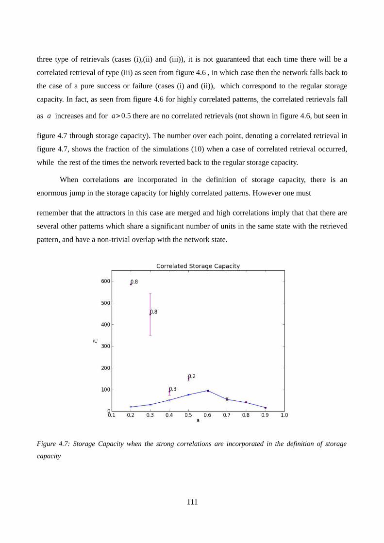
three type of retrievals (cases (i),(ii) and (iii)), it is not guaranteed that each time there will be a

correlated retrieval of type (iii) as seen from figure 4.6 , in which case then the network falls back to

the case of a pure success or failure (cases (i) and (ii)), which correspond to the regular storage

capacity. In fact, as seen from figure 4.6 for highly correlated patterns, the correlated retrievals fall

as a increases and for a>0.5 there are no correlated retrievals (not shown in figure 4.6, but seen in

figure 4.7 through storage capacity). The number over each point, denoting a correlated retrieval in

figure 4.7, shows the fraction of the simulations (10) when a case of correlated retrieval occurred,

while the rest of the times the network reverted back to the regular storage capacity.

When correlations are incorporated in the definition of storage capacity, there is an

enormous jump in the storage capacity for highly correlated patterns. However one must

remember that the attractors in this case are merged and high correlations imply that that there are

several other patterns which share a significant number of units in the same state with the retrieved

pattern, and have a non-trivial overlap with the network state.

Figure 4.7: Storage Capacity when the strong correlations are incorporated in the definition of storage

capacity

111

4.7 Modification of learning rules:

The storage capacity that we saw in the previous section was studied with the standard

learning rule (e4.2), restated below

J ijkl =

c ij

Ca(1− aS )∑μ=1

p

(δξiμk−

aS)(δξ j

μl−aS)×(1−δk0)(1−δl0) ... (LR1)

From the signal and noise analysis we saw that as more and more patterns are stored in the network

there is an increasing interference amongst the patterns which limits the number of patterns that can

be successfully stored and retrieved.

One aspect of this learning rule is the term aS

which is subtracted from both the pre and

post synaptic terms. A detailed analysis of the significance of including this term, for a standard

Hopfield network, is done in [Amit, Gutfreund, Sompolinsky 1987]. Since the Hopfield model is

only a two-state spin system, just subtracting a is required, whereas for an S state system the

natural modification to this term is aS

. This term has an effect of reducing the effect of the bias in

the patterns and making the noise term in (e4.4) to have a 0 mean and thus improving the storage

capacity.

4.7.1 'Popularity' subtraction:

Subtraction of the bias term is effective when there are no systematic correlations between

patterns and the overlaps between patterns are only at chance level. With the introduction of

systematic correlations however, as we do with our pattern generation algorithm for low and high

correlations, just subtraction of the aS

term is not sufficient. In the case of a standard Hopfield

model, this problem was investigated in [Kropff, Treves 2007]. Instead of subtracting a from the

pre and post synaptic terms, they subtract what is called the 'popularity' of the neuron, defined as

112

the average activation of that neuron over all the stored patterns. Here we extend that definition to

the Potts units and write the 'popularity' term as

aik=⟨ξik ⟩μ ;where ⟨a ik⟩=aS

with this we write the modified learning rule as

J ijkl=A∑

μ=1

p

(δξiμ k−aik)(δξ j

μl−ail)×(1−δk0)(1−δl0) ...(LR2)

Thus the reduction of bias while storing the patterns is more refined rather than using a single mean

value of aS

, and it depends on the specific set of patterns being stored, thus affecting the storage

capacity. We shall see the effect of this modification after the following section, where we look at

another modification to the learning rule.

4.7.2 Constrained synaptic modification:

From the noise profile in section 4.4 we saw how the distribution of noise gets more and

more positively skewed as correlations amongst patterns increase. This is in effect due to the high

contribution of the positive terms in the summation of the noise over all the stored patterns: the

positive contributions arise from the increased positive overlaps that result due the stronger

correlations between patterns. Since the source of these excess positive contribution is in the

synaptic connectivity matrix, J ijkl , we intend to mitigate this effect by modifying the synaptic

strength between two units, on each successive presentation of a new pattern to be stored,

proportionally to the existing strength of the synaptic connection between the units that the pattern

modifies. The rule is written as,

J ijkl{q}=J ij

kl{q−1}+(δξ i

μ k−aik )(δξ jμ l−a il)e

−α Jijkl {q−1}(δξi

μk−aik)(δξ j

μl−ail)

for the qth pattern ,q=1,2... p

...(LR3)

Thus the change in the synaptic strength between units i and j is moderated by an

113

exponential function whose exponent is a scaled product of the existing synaptic strength,

J ijkl{q−1} , and the change due to the new inputs it receives, (δξi

μ k−a ik)(δξ jμ l−ail) . If the new

inputs strongly affect a synapse that is already strong, then the influence of these inputs on that

synapse drop exponentially. This drop can be controlled by the parameter α , setting α=0 one

gets back LR2. One must note that reducing the influence of new inputs also reduces, in fact, the

information content about the new inputs, thus one cannot set α⩾0 , otherwise the patterns will not

be stored in the network. Through simulations we find that for highly correlated patterns the value

of α which results in the desired effect of reducing the spread of noise and increasing storage

capacity is α=1 at a=0.2 while for a>0.2 and the low correlations case we see the intended

effect at α=0.01 for all a (figure 4.10) . This learning rule is local, biologically plausible and

makes on-line modifications during learning.

4.7.3 Effect of modified learning rule on noise profile:

Similar to section 4.4 we look at how the standard deviation and skewness of the noise

distribution is affected by the two modifications mentioned in the previous two sections. Figure 4.8

shows, overall, that LR2 (dotted line) and LR3 (dashed line) effectively reduce the standard

deviation and skewness of the noise distribution compared to LR1 (solid line) for the high and low

correlations cases, while there is no significant change in the case of random patterns.

For the high correlations case there is a marginal reduction in the standard deviation due to

LR2 and a slightly greater reduction for LR3, except at a=0.2 where there is a stronger reduction

in LR3. For the low correlations case the reduction in standard deviation is comparable for both

LR2 and LR3, at a similar level lower than for LR1, while for the random patterns all three learning

rules are comparable. If we look at the skewness, the pattern is similar for high correlations as

mentioned above, while the skewness for the low correlations case is brought down to the level of

random patterns.

114

Figure 4.8: Reduction in standard deviation and skewness (as a function of sparsity) brought about by themodification of the learning rule, LR2 and LR3.

115

Figure 4.9: Reduction in standard deviation and skewness (as a function of storage load) brought about bythe modification of the learning rule, LR2 and LR3.

A similar effect of reduction in standard deviation and skewness is seen as a function of

network load p. LR3 however has a more pronounced effect in this case, as seen from the 3rd panel

in figure 4.9, where the product of standard deviation and skewness which linearly rises for the high

correlations case is made, instead, comparable to the low and random correlations cases by the

application of LR3.

4.8 Storage capacity with modified learning rule:

From the results of section 4.7 we expect the storage capacity to be slightly higher than what

we saw in figure 4.3, which is indeed the case as shown in figure 4.10 (pto).

116

Figure 4.10: Storage capacity as a function of sparsity for the three learning rules LR1, LR2 and LR3(see text)

Both LR2 and LR3 show an increase in the storage capacity for high and low correlations.

The change is stronger in the case of low correlations which can be partly understood by the

lowering of skewness for low correlations in figure 4.8. There is no big difference in the storage

capacities between LR2 and LR3, with LR3 resulting in only a very marginal higher storage

capacity as compared to LR2. A noticeable difference is seen at a=0.2 for the highly correlated case

in LR3 which corresponds to the change seen in figure 4.8. None of the modifications however

sufficiently reduce the interference due to correlations so as to increase the storage capacity to a

comparable level with the random patterns case. LR3 in the case of random patterns, in fact, causes

a slight lowering of the storage capacity, due to the fact that the correlations in the random cases are

so low that any suppression of the inputs on the basis of correlations in turn results in the lack of

information about the entire pattern. A similar effect is seen in the region of a>0.6 , where LR2 and

LR3 result in lowering of storage capacity as compared to LR1. This is due to the subtraction of the

popularity term, which becomes strong with increasing a and destroys information about the

pattern.

117

4.9 A self-excitation trick to store more patterns:

We saw how interference from the stored patterns other than one being retrieved puts a limit

to the maximum number of patterns that can be stored. This can be seen from the separation of the

signal and noise terms in (e4.4). What happens if the signal is enhanced by an external input to the

field, which makes it stronger than the interference from noise?

To recall (e4.3) , the field on each unit is given by

hik=∑

j≠i∑l=1

S

J ijklσ j

l+w(σi

k−

1S∑l=1

S

σil)

here 'w' as explained chapter 4 section I-C, controls the self excitation of the unit and boosts the

field in the direction of the signal. The results so far were obtained by setting w=0 and not having

any self excitation. We now set w=0.8 thus making the signal stronger and looking at how the

storage capacity is affect by this change.

Figure 4.11: Storage capacity when signal is boosted by self reinforcement (w=0.8)

The effect of rising sparsity, a , which lowered the storage capacity, seems to be nullified

in the case of random and low correlation patterns. The increasing spread of noise with increasing

118

sparsity does not affect the boosted signal and the storage capacity remains more or less constant as

a function sparsity at the level which corresponds to the higher storage capacity at a=0.2 in

figure 4.10 for LR2 and LR3. Highly correlated patterns show a peculiar behaviour in the region

a>0.5 , there is a monotonic rise in the storage capacity, which becomes greater than the low

correlated patterns and approaches the random patterns as a approaches 0.9. One may try to

partly understand this behaviour from figure 4.4, for a>0.5 the standard deviation of noise for

the high correlations case continues to drop, although at a much lower rate as compared to

a⩽0.5 . This is in contrast to the high and low correlations case, for which the standard deviation

rises with a over the entire range. In fact at a = 0.9 both the standard deviation and skewness for

highly correlated patterns is close to the random patterns and lower than low correlation patterns.

Thus self excitation has a higher impact on the high correlation patterns because of decreasing

standard deviation and in the case of random and low correlations the effect of increasing standard

deviation is balanced out by self excitation.

4.10 Discussion:

We presented an algorithm which generates patterns of various levels of correlations. These

patterns are intended to represent the activity of local cortical patches and together represent the

activity over the the entire cortex. Thus each pattern ξμ , is expected to be a stored memory

which can be recalled when the right cue is presented. Since each unit in the pattern can be in

several possible states and that there are several such units, a 'memory' of any particular object is

thought be entailing its entire multidimensional aspects. Different objects can share various levels

of correlations along several dimensions in the natural world. Thus it is important to study how

correlations affect the storage of correlated memories in the Potts model.

Our long term aim is to store syntactic-semantic relations of words into the Potts network

and we saw the first attempt at it in section I-E, [Primoradian 2012]. The words presented in that

119

study shared a near random correlation but in future the aim is to introduce corpus-frequency based

correlations amongst words.

Correlations severely limit the ability to store patterns in the Potts network. We saw that the

signal becomes weaker in comparison to interference (noise) from other stored memories when

correlations between the memories increase. Increasing noise drastically reduces the storage

capacity for highly correlated patterns. By looking at the three different retrieval behaviours of the

network for different level of correlations we decided to relax the definition of a successful

retrieval and take into account the strong correlations amongst patterns. In doing so, we saw that

the network could retrieve its maximum storage capacity around the level of random patterns but

only for a low level of sparsity.

Modifying the learning rule based on the signal-noise analysis lead to a very marginal

improvement in the networks ability to store correlated patterns. The increase in storage capacity

due to LR2 and LR3 was more pronounced for the highly correlated patterns at a=0.2 , with

LR2 resulting in close to 1.4 times rise in the storage capacity while LR3 resulting in a rise of close

to 2.7 times that of LR1. However, since the storage capacity is already so diminished for high

correlations the increase too is small.

Storing correlated memories in a neural network, especially of the type as generated by our

algorithm which intends to mimic natural correlations is a challenging task and certainly a crucial

one in the context of language processing.

120

Chapter 4

Section III

Towards the Possibility of the Potts Glass Phase

4.11 On the glass phase of the Potts Neural network:

The Potts model, as described in section I-C, aims to model the interaction of several local

modules in the cortex, where each module is represented by a Potts unit which can assume S

different states. This is an N-body interaction system ( N≫1 ), with infinite range interactions,

which implies that a local unit i is not restricted to interact with only its neighbouring units but

can interact with all other units in the system, with an interaction strength J ij . Such systems,

when the interactions are complex, or not following any simple ordering, are known to exhibit a

rich variety of complex behaviour, one of which is the existence of a spin glass phase. A spin glass

phase can be described as the typical low-excitation state of a system of interacting spins that

exhibits both quenched disorder and frustration. In a relatively simpler case where each unit has

only two possible spin states of + or – (Ising Spins), quenched disorder stands for a random

distribution of 'ferromagnetic' and 'anti-ferromagnetic' interactions. This simply means that

individual pairs of spins are either favoured to be aligned in the same direction or in the opposite

direction, and such influences are 'quenched', i.e do not evolve with time. Thus on average, spin

interactions cancel each other out. 'Frustration' in a spin system is when no spin arrangement of all

the units completely satisfies all the couplings between the spins. The effect of unit i on j ,

determined by J ij , contributes to the alignment of unit j, but unit j receives such orienting forces

from many other units. In a frustrated system the spins get 'frozen' such that not all the interacting

forces are satisfied by the final spin orientation of the unit j . This spin glass phase typically

leads to multiple, possibly infinite different arrangements of spins and hence to a multitude of stable

and metastable degenerate energy states.

121

Since it is a general property of disordered many body interacting systems, and we suppose

the cortex, at least as a first order assumption, to fall under this category, it can be subject to

investigation whether the cortex too, exhibits a spin glass like behaviour . The existence of

frustration and multiple degenerate states makes it a particularly interesting problem when one

thinks of rule learning and structured interactions between various domains in the brain.

4.11.1 Suggestions from the mean field models of the spin glass phase:

Spin Glass properties of interacting spins were originally studied in the scope of magnetic

materials but soon the importance and application extended to various other N-body systems.

[Sherrington and Kirkpatrick, 1975] proposed a mean field theory of spin glasses with infinite range

interactions (SK model), which was an extension of the finite range Edward-Anderson model. An

important mathematical tool was developed for this purpose called the 'Replica Trick', which makes

possible to calculate the mean free energy of the system and hence further make a phase study

analysis. Without going in details, the replica trick involves calculating the partition function,

Z=∑s

e(βH s) , of n replicas of the system and then take the limit n→0 using the identity,

log Z=limn→0

Zn−1n

. The free energy is defined as F=−T ln Z (where T represents the

temperature of the system). The SK model develops the solution in the replica symmetry

assumption, where the n replicas are perfectly symmetric, however this leads to a negative entropy

in the n→0 limit. As a solution [Parisi 1979, 1980] proposed a model by introducing an ansatz

and breaking the replica symmetry which solves the negative entropy problem. Importantly, a

notable result is that the low temperature solution shows a phase transition below a certain critical

temperature, T c , to the spin-glass phase of infinite degenerate states, in the system of infinite

range interacting Ising spins.

[Gross, Sompolinsky 1985] developed the mean field theory of Potts glass where they

122

found a continuous transition to two distinct glass phases for number of states S⩾3 , at low

temperatures below the critical temperature T c . The first one at T<Tc , (PG1), with infinite

pure degenerate states which do not overlap with each other and the second one (PG2) at T2<T c

where each of the pure state in PG1 splits into a hierarchical structure of partially overlapping

states. For S >4 the transition becomes discontinuous.

4.11.2 Glass phase in the Potts neural network model:

Our model, which is specifically designed to address cortical dynamics, has a neural

network structure and differs from the models mentioned above in three aspects,

a) The interaction term J ij is a result of associative learning as determined by the specific

patterns that are stored in the network. Importantly, the way in which we define the learning rule,

the J's do not follow the full symmetry of J ijkl=J ji

lk . Whereas in the models discussed above, J's

are decided by a Gaussian probability function with a specific mean and standard deviation.

b) The Potts units in our model are graded and the final state σik is determined by a

continuous transfer function applied to the fields, allowing a graded response in the units unlike the

123

completely discrete units of above mentioned models.

c) An important distinction in the dynamics of our model is the definition of 'active' and

'inactive' states which have separate dynamics. Learning occurs only with the active states to

remain in the biologically plausible scenario.

[Bolle et al 1992] studied the mean field solution of the S state Potts glass neural network

model where the phase is investigated in Temperature-Storage capacity space. Though the model

discussed by Bolle et al still differs from ours in all the three points mentioned above, nevertheless

it sheds light on the spin glass phase of the Potts neural network and it reveals the rich behaviour of

this class of networks. Among the findings of this study, they show that there exists a critical

temperature T g , below which the network exhibits a spin glass phase which consists of states

that share no overlap with the stored states. Another transition occurs at T M<T g , where the states

have a finite overlap with the stored patterns. Thus the stored patterns are local minima of the free

energy and the network can function as an associative memory, and below T M the stored

patterns become a global minima of the network.

It is likely that there exists a spin glass phase in all such models of large interacting systems

and in the limit that the brain can be modelled as a system of many interacting neurons/modules,

this becomes an important characteristic which may influence cognitive function.

4.12 Indication of spin glass phase in the 'cortical' Potts model:

We explore the glassy nature of our model by examining the final steady state energy values

that the network evolves into. In the usual attractor dynamics, the network settles at the bottom of

the energy valley of a particular attractor which is designed to be one of the stored memory patterns.

However in a spin glass situation the network can have multiple stable energy states brought about

by the interactions of various units. We calculate the energy of the network state or pure pattern

with the standard formulation with an addition for graded units,

E=−12∑i , j≠i

N

∑k ,l=1

S

J ijklσ i

kσ j

l+∑

i

N

∑k=1

S

(U σ ik+

1β(σi

k lnσi

k

σik+σ i

0+σ i0 ln

σi0

σ ik+σi

0 ))

124

where the first two terms denote the interaction energy and the contribution of the fixed threshold

respectively, while the last term is the contribution due to the fact the Potts units are graded

[Russo,Treves 2012].

We first look at the scatter of energy levels of the pure patterns and the stable network state

when a pattern was cued to the network for retrieval. As in section 5.4 we separate the three

different retrieval behaviour by the same colour code of green,red and yellow for case(i), case(ii)

and case(iii) respectively. Figure 4.12 plots the energy of the pure pattern (triangle) for each of the

pure pattern ξμ , μ=1,2... p . p is set around the storage capacity level so the network can

exhibit the different types of retrievals. Along with the energy of a pure pattern, the energy of the

final network state when a particular pattern ξμ is cued to the network is represented with a

cross.

We see that the steady network state energies do not coincide with the pure pattern energies

and find a multitude of energy valleys to settle in. The network either settles in a region above the

desired valley and yet have a successful retrieval in the retrieval type of case(i) or find an energy

state below the pure pattern. This is an indication of a typical property of the spin glass phase, in

which there are high number of metastable states due to the formation of multiple local minima,

resulting from several possible spin interactions. One clear phenomenon seen is that whenever the

network fails to retrieve, either case(ii) or case(iii), it almost certainly settles in a state lower than

the cued pattern as seen clearly in figure 4.13. Thus it falls out of the desired attractor and finds a

basin with a lower energy, leading to a failure in correct retrieval. This observation is consistent

across the different levels of correlations amongst patterns. The failed network states are all on the

same level for random patterns because this is the inactive state of the network and for unsuccessful

retrievals the network decays into inactivity. Same is the situation for low correlation patterns but

in this case the network decays into a mixed state with several patterns having a finite overlap with

the network state. In the case of highly correlated patterns, there exist situations where the network

settles into at the level of pure pattern energy level. An interesting observation in the case of random

patterns is that the pure patterns which are lower in energy than the mean energy of patterns, are

retrieved successfully while those above fail. This clear separation is not seen in the other two cases

of correlated patterns.

125

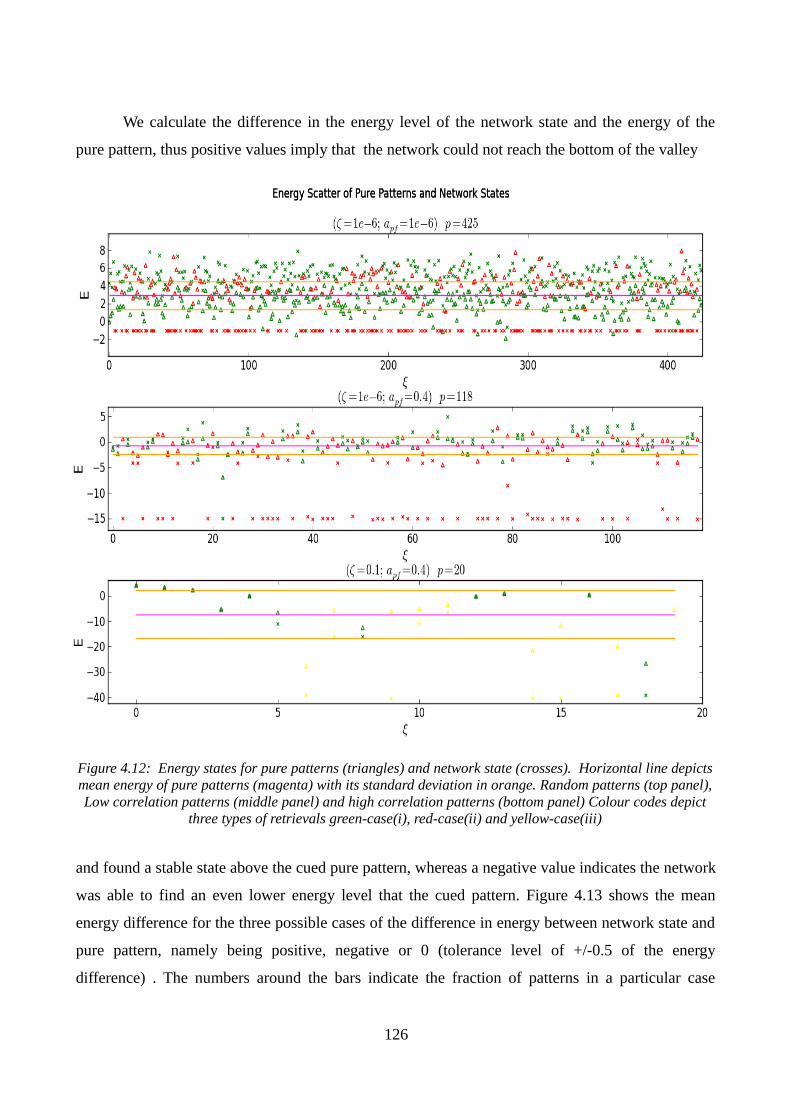
We calculate the difference in the energy level of the network state and the energy of the

pure pattern, thus positive values imply that the network could not reach the bottom of the valley

Figure 4.12: Energy states for pure patterns (triangles) and network state (crosses). Horizontal line depictsmean energy of pure patterns (magenta) with its standard deviation in orange. Random patterns (top panel),Low correlation patterns (middle panel) and high correlation patterns (bottom panel) Colour codes depict

three types of retrievals green-case(i), red-case(ii) and yellow-case(iii)

and found a stable state above the cued pure pattern, whereas a negative value indicates the network

was able to find an even lower energy level that the cued pattern. Figure 4.13 shows the mean

energy difference for the three possible cases of the difference in energy between network state and

pure pattern, namely being positive, negative or 0 (tolerance level of +/-0.5 of the energy

difference) . The numbers around the bars indicate the fraction of patterns in a particular case

126

(positive- above the bar, 0-beside the bar at 0 level, negative-below the bar) . The three types of

retrieval behaviours are shown in their defined colours. Figure 4.13 makes it clear that failures

always find a range of stable network states below the pure pattern while the majority of the

successful states are when the network is trapped in the energy valley of the cued pattern but above

the pure pattern energy level. One may speculate that the tendency of the network is to fall out of

the energy valley towards an attractor with a deeper energy valley but probably frustrated frozen

spins trap the network in the valley while for failures it manages to fall out.

Figure 4.13: Mean difference in energy between network state and pure pattern. Numbers indicate fractionof patterns in each condition (see text) represented by the width of the bar.

127

4.13 Effect of local module temperature:

The parameter β intends to represent a local module inverse temperature and in effect

controls the noise level within a unit over its various states. Low values of beta, implying high

temperature would make the units very noisy and hence none of its states would be dominant. On

the other hand at very low temperatures, high β , the state having the highest local field will

essentially coincide with the final state of the unit while all other states will become 0, representing

a noiseless situation. Thus at high β the Potts units become in practice non graded. We test how

the above mentioned spin glass effects are affected at different local module temperatures. The

results of the previous section were obtained at β=11 , which represents a medium noise level

which still allows the network to function as an associative memory. Now we test the extreme limits

of very high temperature at β=5 and very low temperature, β=100 , which makes the Potts

units, in practice non graded.

128

Figure 4.14: Mean difference in energy, same as figure 4.13 but for three different values of β - 5

(top), 11 (middle) and 100 (bottom) panel, in random patterns

At high temperature β=5 , a retrieval becomes highly improbable since the units can not

be kept in the state with the highest local field. This results in an almost total failure to retrieve

with only one pattern retrieved, in which shows the network settles much below the pure pattern

energy. In the noiseless case β=100 ,by contrast 99% of the patterns are successfully retrieved.

Importantly the spin glass behaviour is present also when the units practically behave a non graded

129

manner. A similar trend is seen for low and high correlation patterns (figures 4.15 and 4.16). As

seen before (figure 4.13) the failures in high correlation patterns are of the type(iii).

Figure 4.15: Mean energy difference for three levels of local noise, β=5 (top), β=11 (middle) and

β=100 (bottom), in low correlation patterns.

130

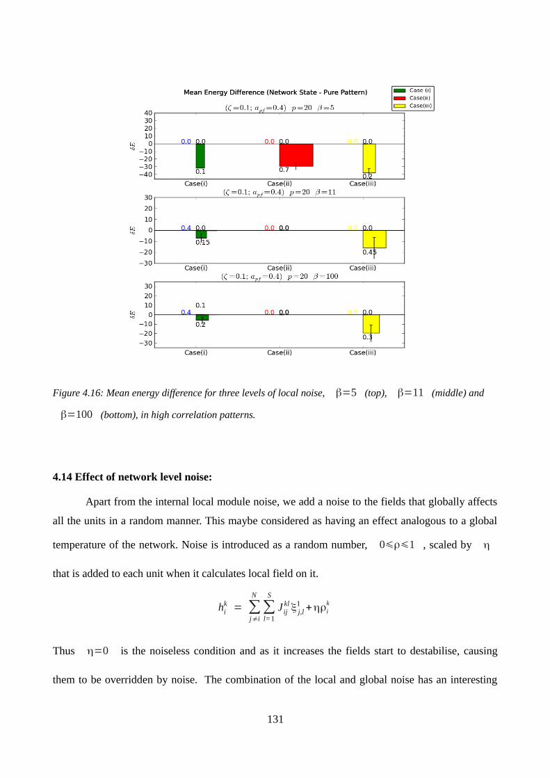
Figure 4.16: Mean energy difference for three levels of local noise, β=5 (top), β=11 (middle) and

β=100 (bottom), in high correlation patterns.

4.14 Effect of network level noise:

Apart from the internal local module noise, we add a noise to the fields that globally affects

all the units in a random manner. This maybe considered as having an effect analogous to a global

temperature of the network. Noise is introduced as a random number, 0⩽ρ⩽1 , scaled by η

that is added to each unit when it calculates local field on it.

hik = ∑

j≠i

N

∑l=1

S

J ijkl ξ j,l

1 +ηρik

Thus η=0 is the noiseless condition and as it increases the fields start to destabilise, causing

them to be overridden by noise. The combination of the local and global noise has an interesting

131

effect on the random patterns as we can see in figure 4.15.

Figure 4.17: Fraction of patterns successfully retrieved as a function of external noise, η . For two

different values of β=11 (full), β=100 (dashed)

When β is high, the fraction of patterns that is successfully retrieved, rapidly decays as

noise increases, with a sigmoid like function. This fits the intuitive notion of how noise may affect

retrievals, because it randomly reorients the units thus dominating over the inputs from the synaptic

connections. However at β=11 , when the units are graded there is a maximum in the fraction of

successful retrievals at η=0.075 , with a rapid decay for η>0.1 . Overall the combination of

both local and global noise results in a higher success rate for η>0.05 . As one might expect,

when both the internal and external noise levels are low ( β=100 , η=0 ), the network has the

best retrieval rate.

As before we calculate the mean energy difference between network state and pure pattern

for the global noise η in figure 4.18. but now we calculate the total mean instead of separating

132

the positive and negative differences. In the case of high β , β=100 , the mean difference in

the energy is positive and increases monotonically with η . Hence the network finds it

increasingly difficult to

Figure 4.18: Influence of external noise η on the total Mean difference in energy.

reach the bottom of the energy valley when noise is increased. In the case of β=11 , instead there

seems to be a region around η=0.075 , where the effects of the two types of noises prove

beneficial for the network to reach closer to the energy valley of the pattern, seen as a reduction in

mean energy difference. For η<0.075 the medium internal noise units ( β=11 ) have a

difficulty in reaching the energy bottom as compared to the noiseless units ( β=100 ), thus

resulting in lower fraction of successful retrievals in figure 4.17. Having graded units with a small

global random noise helps in better retrieval of patterns as seen through the lower mean energy

difference for β=11 as compared to β=100 , in the region η⩾0.075 .

133

This combined effect of global and local noise to cause an increase in successful retrievals

is seen only for the random patterns and is absent in low correlation patterns, where the fraction of

successful retrievals monotonically reduce with η (figure 4.19). The low correlation case seems

to follow the intuitive expectation that low internal noise units β=100 will tend to have better

retrieval ability and thus lead to higher number of patterns retrieved as compared to β=11 .

Figure 4.19: Fraction of patterns successfully retrieved as a function of external noise, η . For two

different values of β=11 (full), β=100 (dashed) in low correlation patterns.

4.15 Behaviour at low S and full connectivity:

With cues from [Gross et al 1985] where they find a distinction in the phase transition at low

S and S > 4, we reduce the number of states to S=2 to check if we find the same behaviour of

the network as in the case of S=5 investigated before. In addition we test the behaviour when the

network connectivity is increased to a fully connected network and eliminate effects of dilution,

134

thus Cm which is 90 in previous cases is increased to 599 (N=600). In both cases the local

inverse temperature β is set at mid-level of β=11 .

Figure 4.20 confirms the spin glass nature of the 'cortical' Potts network in low S and also in

a fully connected case. Apart from the fact that there is a higher fraction (0.11) of patterns in which

the network reaches the bottom of the energy valley of the cued pattern for S=2,Cm=90 , when

compared to S=5,Cm=90 , there are no major differences. For Cm=599 the network settles

in a varied range of levels during successful retrievals below the cued pattern energy level thus

finding a better configuration of spins which reduce the energy of the network and yet retrieve the

intended pattern.

Figure 4.20: Mean difference in energy, same as in figure 4.13, but for S=2 , Cm=90 (top) and

S=2 , Cm=599 (bottom) panel

135

4.16 Brief Discussion:

The human cortex is estimated to have 109 neurons [Herculano-Houzel S 2009] and an

order of 1014 synapses. As described in section I-C we model the cortex as N interacting Potts

units, each of which represents a patch of the cortex, that can be in S possible attractor states,

resulting in a system of N interacting S state spins . It has been shown that at low temperatures a

system of large N interacting spins exhibits a spin glass phase. A spin glass phase has multiple

degenerate energy states and has a 'frustrated' spin configuration. This allows the network to settle

in varied energy states with different spin configurations. If we assume that a simplified version of

cortical dynamics can be modelled by the Potts neural network then it is possible that the cortex

may function in a spin glass like manner.

We found that the Potts neural network does show signs of a spin glass like phase by

allowing the network to evolve after an initial cue and update its unit as prescribed in section I-C.

The network settles into multiple energy states which are either higher than the energy of the pure

pattern or lower. In the case of successful retrievals, the network predominantly settles in a higher

energy state as compared to the pure pattern energy but the fact the retrieval is successful implies

that the network is in the correct energy valley. Since there is a difference in the two energy levels

of the network state and pure pattern, it implies that not all the Potts spins are aligned with the pure

pattern and some of them are 'stuck' in the attempt of the network to find a suitable energy level.

Since whenever the network fails to retrieve it almost always settles in a state lower than the pure

pattern, and these failed states are the lowest amongst all other states. Thus it is possible that the

Potts spins in a successful state get 'frozen' in the networks attempts to settle in a lower global

minima than the 'successful' higher local minima and hence leading to the observed positive energy

differences between the network state and pure pattern.

Spin glass like characteristics that were seen with a diluted network connectivity, Cm=90

and medium internal noise β=11 at S=5, were also consistently observed in the low S=3

condition, full connectivity, Cm=599 and a near absent internal Potts unit noise β=100 .

Adding a small amount of external global noise combined with the medium level of internal noise

seems to facilitate the network, to reach the energy valley bottom. This can be seen through the

136

reduction in energy level difference between the network state and pure pattern. As a result it leads

to a higher fraction of patterns that are retrieved successfully. One possibility is that a small external

noise at , does not destabilise the unit but is sufficient enough so that it overrides the interaction

forces that cause misalignment amongst units.

The effects of spin glass behavior in the Potts neural network and its application to cognitive

process is yet unexplored but provides an exciting opportunity to study how structured transition

between stored memories may occur in a dynamical scenario. Since spontaneous transitions

between memories are largely driven by the energy landscape, the spin glass nature of the Potts

network may influence the transitions. Structured transitions between memory 'objects' constitute a

formal rule and hence the spin glass effects may play a role in language processing too.

137

5 A Report on the Effect of Learning Rules on Latching

Dynamics

5.1 Latching behaviour for increased correlation between patterns

In chapter 4, section I-D we mentioned the dynamic behaviour of the Potts neural network,

in which the network exhibits latching (spontaneous transition from one stored memory to another).

Latching occurs due to the time varying thresholds ( θik and θi

0 ), which destabilise the units

once the network has reached a stable attractor state and thus eventually cause the network to fall

out of the attractor. However, as the network is falling out of the attractor it may be driven towards

another attractor which has its basin of attraction in the proximity of the previous attractor. The

temporal scale of network dynamics is governed by three time constants,

(i) τ1 – time constant in which the local field experienced by each unit in its active states is

integrated, subject to the time varying threshold; (ii) τ2 – the time constant with which θik ,

the threshold affecting only the active states, updates itself and (iii) τ3 – the time constant for

updating θi0 , the threshold expressing the effect of slow inhibition. The specific dynamics are

governed by the equations mentioned in chapter 4, section I-C.

An analysis of the storage capacity in chapter 4, section II was worked out considering the

asymptotic steady state behaviour of the network. For that purpose τ2 and τ3 were effectively

set to ∞ , thus removing the adaptive nature of the Potts units. We now consider the network in

what is termed as the slow adaptive regime, referring to the situation in which neuronal dynamics is

138

much faster than the threshold dynamics. This is obtained by setting τ3> τ2≫τ1 for finite a τ2

and . τ3 [Russo, Treves 2012] studied the latching properties of the network using random

patterns in the slow adaptive regime as a function of various parameters like the self-excitation term

w , storage load p , local temperature T , connectivity dilution Cm and the time

constants. One of the observations of interest was that the network tends to latch between patterns

that have an above average correlation amongst them. However we have seen in section II that

increasing the strength of the correlations drastically affects the behaviour of the network in terms

of its stable retrieval ability of stored patterns. We now focus our attention on the dynamical

behaviour of the network when the patterns are highly correlated and present a preliminary study

with some immediate observations.

5.2 Effect on latching due to different learning rules:

The network is tested in the 'infinite latching' phase, which refers to the situation when the

network does not stop latching for the entire duration of our simulation (5000 time steps). The

asymptotic stability of a stored pattern during its retrieval and thus the critical storage capacity of

the network has a limited impact on latching dynamics due to the non-stationary nature of retrieval

in the latching phase. Latching is however, sensitive to the strength of correlations amongst

patterns. We load the network with 200 patterns and record the latching transitions (consecutive

pairs of patterns that have the highest overlap with the network state across a transition) using the

three learning rules LR1, LR2 and LR3, described in section II-4.7. In the case of random patterns

latching was seen to occur only for w>0 [Russo, Treves 2012], however in the case of highly

correlated patterns we see continuous and spontaneous activity at w=0 (figure 5.2-(i),(ii)).

139

figure 5.1- Latching statistics for high correlation patterns using the learning rules LR1, LR2 and LR3.

(see text for details)

When the patterns are highly correlated there does not seem to be 'proper' latching in the

network (using LR1 and LR2) even though the network shows spontaneous activity. The network

appears to be stuck in a mixed attractor (figure 5.2-(i) and (ii)) and keeps oscillating between highly

correlated patterns without a transition into another pattern. However with the application of LR3

this cycle is broken, allowing the network to visit other patterns and exhibit 'proper' latching (figure

5.2-(iii)). The top row of figure 5.1 shows the correlation scatter of all the pairs of patterns (just as

in figure 4.2a) but with an overlay of latching pairs (in red). The three columns represent plots for

the three different learning rules. Most of the latching happens between pairs that share a correlation

of around Nas=10 (2nd row figure 5.1) which is midway between no correlation ( N as=0 ) and

the pairs with maximum correlation ( N as=20 ).

140

We calculate the entropy of latching, which quantifies the diversity of patterns visited during

the latching sequence. Thus low entropy would indicate the network is stuck between a few patterns

and an increase in entropy would imply that network is visiting more patterns during the latching

sequence. The entropy was 0.05, 0.04 and 0.53 for LR1, LR2 and LR3 respectively. The mean

active length - the time a pattern stays active with the highest overlap during latching is 168.72 and

226.77 time steps (in a total of 5000 time steps), for LR1 and LR2 respectively. This indicates that

the highest active pattern, in the case of highly correlated patterns, shows resistance to decay and

stays active for a longer period of time as compared to low and random correlations (figures C and

D), for which the mean active length is in the range of 44 to 79 time steps. LR3 however, for highly

correlated patterns, facilitates transitions to other patterns and brings down the mean active length

to 17.75 time steps.

LR3, with its proportional suppression of high correlations during the storage of patterns,

brings about a separation in the energy valleys of stored memories, which otherwise in the case of

high correlations are merged into each other with strong overlaps. Thus we can restore the latching

behaviour of the Potts network for highly correlated patterns.

Below, in Figures B (i), (ii) and (iii) in overlap of each pattern with the network state is

plotted against time (shown for first 1500 time steps). As the network transits from one attractor to

another, the respective patterns for those particular attractors have the highest overlap with the

network. The overlap is measured as,

mμ=1

Na(1−a/ S)∑j≠i

N

∑l=1

S

(δξ jμ , l−a /S)σ j

l

(all symbols have their usual meaning, as described in section I-C)

141

Figure 5.2-(i): Latching transitions using LR1. The network activity is mainly dominated by two patterns

which do not show a complete decay

Figure 5.2-(ii): Latching transitions using LR2. The network activity is mainly dominated by a single pattern

which does not show a complete decay

142

figure 5.2-(iii): Latching transitions using LR3 with α=1 . The network latches between various

patterns.

Rest of the parameters, as described in chapter 4, section-I-C have the values of, N=600

, S=5 , a=0.2 , U=0.2 , τ1=2 , τ2=102 , τ3=106 , Cm=90 and β=11 ,

w=0 .

We now record the latching statistics, i.e. the same as in figure 5.1 but for low and random

correlations, shown in figure 5.3 and D, with all the network parameters kept the same except w,

which is set at w=1 in order to be in the infinite latching phase. The pattern generation

parameters for low and random correlations are the same as in section II-4.2. The dynamical

behaviour of the network for low correlations and random correlations is very similar to each other.

The phase transitions in the w−T space are seen to be similar too, although at different

transition lines [Russo, Treves 2012].

143

From figures 5.3 and 5.4 we see that the three learning rules have only a marginal influence

on latching dynamics when correlations are low.

figure 5.3- Latching statistics for low correlation patterns using the learning rules LR1, LR2 and LR3.

144

figure 5.4- Latching statistics for random correlation patterns using the learning rules LR1, LR2 and LR3.

Overall the entropy increases slightly from LR1 to LR3, thus indicating that more patterns

become accessible to the network during latching. The entropy is highest for highly correlated

patterns with LR3 at 0.53, and on an average it increases as correlations become stronger, from

random patterns to highly correlated patterns. This may be the result of better access to other

patterns, due to the fact that increased correlations cause overlaps between the basins of attraction

of other attractors to increase. Increases in correlations also add a higher positive contribution to the

local field hi of each unit, when J ijkl is summed over all the remaining units and states. This

has an analogous effect to w . Thus the network can exhibit spontaneous activity even at

w=0 for highly correlated patterns, but this also causes the patters to have an increased stability

against the time varying thresholds which hampers the latching process. LR3 suppresses this

145

positive contribution to hi which in turn facilitates latching.

As stressed in section II, correlations are crucial for a model of language processing and

hence it is of much importance that the latching process is preserved when memories are highly

correlated. We showed that the critical storage capacity has only a limited impact on the latching

behaviour and the network does not lose its functional characteristics, in terms of dynamical

behaviour while operating above its storage capacity and using LR3 for highly correlated patterns.

146

6 Conclusions

The broad aim of our study was to explore language mechanisms and in parallel investigate

the properties of a general neural processing apparatus that may help sub serve those language

mechanisms. Keeping the importance of statistical learning in mind, we focussed our investigation,

in part A (chapters 2-3), on the statistical properties of the mass-count distinction between nouns,

which neatly lies on the interface of syntax, semantics and cognitive perception. Language is mostly

thought to be processed in the prefrontal cortex, which is also responsible for other high level

cognitive phenomena [Gabrieli et al 1998; Bookheimer 2002; Bunge 2004], hence stressing the

need to explore models that use general cortical mechanisms to address language processing. In Part

B (chapter 4: sections I-III) we studied some of the features of a neural network, namely the Potts

neural network, intended to model cortical processing in a simplified way, thus attempting to

explore the feasibility of the model to serve the purpose of language processing.

The findings of the second chapter suggest that the mass count syntax is largely left

undetermined by semantic attributes and that one cannot regard it as a binary or quasi-binary

structure. The distribution of syntactic usage properties is very far from bimodal in five out of the

six languages tested. One is led to think of this grammaticalisation as a graded self-organization

process, operating within languages and to some extent within individual speakers, and driven only

to a limited extent by universal attributes, and plausibly governed or at least constrained by

language specific principles. However, at this stage we cannot tell to what degree the

grammaticalisation is governed, beyond the universal semantic or perceptual principles that we

have attempted to quantify, by language-specific principles of different nature, such as cultural

factors, historical accidents, individual language acquisition history, even context dependence

within individual speakers.

With rich multidimensional diversity in the syntax and semantics of the mass-count

distinction and a low cross-linguistic and syntactic-semantic mutual information, it was shown that

a simple self-organising neural network is insufficient to learn a mapping implementing a syntactic-

semantic link. However the network was able to extract the concept of 'count', and to some extent

that of ‘mass’ as well, without any explicit definition, from both the syntactic and from the semantic

data. This categorisation was clear and sharper in the markers than in the nouns. Nouns on the other

147

hand were aligned on a single dimension and showed a graded distribution over the mass-count

spectrum. Thus it seems that even though there is a separation in the mass count divide within the

markers, the application of them to the nouns is variable to a large extent and it is predominantly

context dependent.

In chapter 4-section II, we looked at the ability of the Potts neural network to store

correlated patterns. We expect a model of language processing to robustly handle various syntactic-

semantic correlations amongst the words of a language. This seems to be a sticky problem and the

question of negating the adverse effects on storage capacity due to increased correlations does not

have an easy solution. By incorporating correlations in the definition of storage capacity we are able

to regain the higher storage capacity seen for random patterns at low sparsity. During the retrieval

of a pattern in the high correlations case, along with the cued pattern one or more patterns that are

strongly correlated with the cue also have a high overlap with the network state. One may think of a

scenario where another secondary network layer may be responsible for the fine tuning between

highly correlated patterns to distinguish them and recover the desired pattern.

The possibility of a spin glass phase in the Potts neural network opens up an interesting

window to explore its possible role in cognitive functions. Though this area has not been explored

yet, we may think of a scenario where there are many interacting 'features' that bring about specific

rules through their interactions. Language processing is an ideal candidate for this purpose. One of

the ways to formally analyse linguistic structure is given by 'Principles and Parameters' [Chomsky

1986]. We refer only to the structural analysis of the syntax, in which the syntax of a natural

language is proposed to have general principles (abstract grammar rules) accompanied with a set of

binary parameters that describe the language. The spin glass phase has many stable degenerate

energy states of frustrated spin interactions, thus a particular configuration of spins (which could

represent parameters) may bring about a description of the syntactic rules in a natural language.

Frustration would imply that a certain arrangement of some 'features/parameters' would enforce the

remaining ones to be frozen in a particular state thus possibly shedding light on the correlations

amongst syntactic rules. This also has an implication on the 'Poverty of Stimuli' argument

[Chomsky 1980], which states that the entire grammar of a language is unlearnable purely from

experience due to insufficient stimuli to a learning child. With frustrated interactions, the

knowledge of a limited set of features may help to determine other features without explicitly

experiencing them. The combinatorial possibilities of spin configuration of stable energy states

148

could lead to the generative properties of syntax.

We have touched upon only a small aspect of language processing in this thesis. Not only

are natural languages in themselves quite varied and complex in their nature but so is the question

of how humans acquire and process them using general neural principles. This makes natural

language processing the most fascinating, exciting and challenging aspects of the human brain.

149

Future Directions

The results that we have reported in chapter 2, have been purely statistical, that is to say, we

have reported numbers with no discussion of any of the 1,434 items that make up of data base

(where an item is a token from a particular language plus its particular feature values). An analysis

of patterns within the data base is obviously the next stage in a linguistic analysis. This analysis will

involve investigating whether there are recognizable patterns within the variation which are open to

interpretation, whether there are lexical classes of nouns which function as classes cross

linguistically, and if so how to characterize them. For example, advice, information, and evidence

are strongly count in Hebrew and Italian, and mass in English. Do they behave as a class in other

languages too? However, the results that we have so far already have theoretical implications

relevant for continued research into the semantics and grammatical aspects of the mass/count

distinction, and we conclude by specifying three of them.

Another important factor is the context dependence of the mass-count distinction. Our

results establish that there is no independent semantic content in a noun that can completely

determine its use in the mass-count domain. Thus particular instances of a noun, used in a sentence,

as mass or count are influenced by the information that particular sentence conveys as a whole.

Further investigation is needed in this regard beyond the anecdotal evidence.

In the corpus study (chapter 2, section 2.3.5) we studied the frequency of the nouns with

markers, however to include effects of context one needs to involve higher order frequency

relations of the nouns and markers with other words in a sentence. The artificial language, BLISS is

a useful tool in this regard, to test higher order frequency effects in the mass-count domain.

Subsequently, the Potts network can be tested exclusively in the mass-count domain in its ability to

latch between correct nouns and markers based on higher order frequency correlations.

With that in mind, influence of high correlations on the latching transitions needs to be

studied in detail. Although there is a tendency of the network to latch between correlated attractors,

this remains true in the case of random patterns when the attractors are fairly separated. Latching

behavior when the attractors are highly overlapping and share a wide basin of attraction, needs

careful study as high correlations are a necessary requirement in order to model language

processing.

150

Bibliography

Part A

Baker, M. C. (2008). The atoms of language: The mind's hidden rules of grammar. Basic Books.

Bale, Alan C. & David Barner. 2009. The interpretation of functional heads: Using comparatives to

explore the mass/count distinction. Journal of Semantics 26, 217–252.

Bale, Alan C. & David Barner. 2011. Mass-count distinction. Oxford Bibliographies Online,

http://ladlab.ucsd.edu/pdfs/BB@Oxford.pdf.

Barner, David & Jesse Snedeker. 2005. Quantity judgments and individuation: Evidence that mass

nouns count. Cognition 97, 41–66.

Borer, Hagit. 2005. In Name Only, vol. I: Structuring Sense. Oxford: Oxford Univer-sity Press.

Chiarelli V, Chiarelli V, El Yagoubi R, Mondini S, Bisiacchi P, Semenza C. 2011The Syntactic and Semantic Processing of Mass and Count Nouns: An ERP Study. PLoS ONE

6(10): e25885.

Chierchia, Gennaro. 1998. Plurality of mass nouns and the notion of ‘semantic pa-rameter’. In

Susan Rothstein (ed.), Events and Grammar, 53–103. Dordrecht: Kluwer.

Chierchia, Gennaro. 2010. Mass nouns, vagueness and semantic variation. Synthese 174, 99–149.

Deecke, V. B., Nykänen, M., Foote, A. D., & Janik, V. M. (2011). Vocal behaviour and feeding

ecology of killer whales Orcinus orca around Shetland, UK. Aquatic Biology, 13, 79-88.

Elman, J. L. 1991. Distributed representations, simple recurrent networks, and grammatical structure. Machine Learning, 7:195-224.

Fisher, S. E., & Marcus, G. F. (2006). The eloquent ape: genes, brains and the evolution of language. Nature Reviews Genetics, 7(1), 9-20.

Gillon, Brendan S. 1992. Toward a common semantics for English count and mass nouns.

Linguistics and Philosophy 15, 597–640.

151

Greenberg, Joseph. 1963. Universals of Language. Cambridge, MA: MIT Press.

Grimm, Scott & Beth Levin. 2011. Furniture and other functional aggregates: More and less

countable than mass nouns. Paper presented at Sinn und Bedeutung 16, University of Utrecht. [6–8

September 2011]

Hacohen, Aviya. 2010. On the (changing?) status of the mass/count distinction in Hebrew: Evidence

from acquisition. Proceedings of the 25th Annual Meeting of the Israel Associations for Theoretical

Linguistics, doi: http://linguistics.huji. ac.il/IATL/25/Hacohen.pdf.

Hummel, J. E., & Holyoak, K. J. (1997). Distributed representations of structure: A theory of

analogical access and mapping. Psychological Review, 104(3), 427.

Jespersen, Otto. 1924. The Philosophy of Grammar. London: Allen and Unwin.

Koptjevskaja-Tamm, Maria. 2004. Mass and collection. In Geert Booji, Christian Lehmann and

Joachim Mugdan (eds.), Morphology: A Handbook on Inflection and Word Formation, vol. 2,

1016–1031. Berlin: Walter de Gruyter.

Landman, Fred. 2010. Count nouns, mass nouns, neat nouns, mess nouns. In Barbara H. Partee,

Michael Glanzberg & Jurgis Skilters (eds.), The Baltic International Yearbook of Cognition, Logic

and Communication, vol. 6, 1–67. Manhattan, KS: New Prairie Press.

Landmann, Fred & Susan Rothstein. 2012. The felicity of aspectual for-phrases – Part 1:

Homogeneity. Language and Linguistics Compass 6, 85–96.

Lany, J., & Saffran, J. R. (2010). From statistics to meaning infants’ acquisition of lexical

categories. Psychological Science, 21(2), 284-291.

Link, Godehard. 1983. The logical analysis of plurals and mass terms: A lattice-theoretical

approach. In Reiner B. Bäuerle, Christoph Schwarze & Arnim von Stechow (eds.) Meaning, Use

and Interpretation, 303–323. Berlin: Mouton de Gruyter. [Reprinted in Paul Portner & Barbara

Partee (eds.). 2002. Formal Semantics: The Essential Readings, 127–146. Oxford: Blackwell.]

Markman, Ellen M. 1985. Why superordinate category terms can be mass nouns. Cognition 19, 31–

53.

MacWhinney, Brian. 1995. The CHILDES Project: Tools for Analyzing Talk. Hills-dale, NJ:

152

Erlbaum.

Nicolas, David A. 2010. Towards a semantics for mass expression derived from gradable

expressions. Recherches Linguistiques de Vincennes 39, 163–198.

O’Grady, W. (2008). Innateness, universal grammar, and emergentism. Lingua, 118(4), 620-631.

Panzeri, Stefano & Alessandro Treves. 1996. Analytical estimates of limited sampling biases in

different information measures. Network: Computation in Neural Systems 7, 87–107.

Parsons, Terence. 1990. Events in the Semantics of English. Cambridge, MA: MIT Press.

Pelletier, Francis J. 2010. Descriptive metaphysics, natural language metaphysics, Sapir–Whorf,

and all that stuff: Evidence from the mass-count distinction. In Barbara H. Partee, Michael

Glanzberg & Jurgis Skilters (eds.), The Baltic International Yearbook of Cognition, Logic and

Communication, vol. 6, 1–46. Manhattan, KS: New Prairie Press.

Pires de Oliveira, Roberta & Susan Rothstein. 2011. Bare singular noun phrases are mass in

Brazilian Portuguese. Lingua 121, 2153–2175.

Pirmoradian, S., & Treves, A. (2011). BLISS: an artificial language for learnability studies.

Cognitive Computation, 3(4), 539-553.

Prasada, Sandeep, Krag Ferenz & Todd Haskell. 2002. Conceiving of entities as objects and stuff.

Cognition 83, 141–165.

Raymond, William D., Alice F. Healy & Samantha J. McDonnel. 2011. Pairing words with syntactic

frames: Syntax, semantics, and count-mass usage. Journal of Psycholinguistic Research 40, 327–

349.

Rothstein, Susan. 2010. Counting and the mass/count distinction. Journal of Semantics 27, 343–

397.

Saffran, J. R. (2003). Statistical language learning mechanisms and constraints. Current directions

in psychological science, 12(4), 110-114.

Soja, Nancy N., Susan E. Carey & Elizabeth S. Spelke. 1991. Ontological cate-gories guide young

children’s inductions of word meanings: Object terms and substance terms. Cognition 38, 179–211.

153

Taler, Vanessa, Gonia Jarema & Daniel Saumier. 2005. Semantic and Syntactic aspects of the

mass/count distinction: A case study of semantic dementia. Brain and Cognition 57, 222–225.

Van der Velde, F., & De Kamps, M. (2006). Neural blackboard architectures of combinatorial

structures in cognition. Behavioral and Brain Sciences, 29(01), 37-70.

Wierzbicka, Anna. 1988. Oats and Wheat: The Semantics of Grammar. Amsterdam: John

Benjamins.

Part B

Agliari, E., Barra, A., De Antoni, A., & Galluzzi, A. (2013). Parallel retrieval of correlated patterns: From Hopfield networks to Boltzmann machines. Neural Networks, 38, 52-63.

Amit, D. J. (1992). Modeling brain function: The world of attractor neural networks. Cambridge University Press.

Amit, D. J., Gutfreund, H., & Sompolinsky, H. (1987). Information storage in neural networks with low levels of activity. Physical Review A, 35(5), 2293.

Baayen, R. H., Milin, P., Đurđević, D. F., Hendrix, P., & Marelli, M. (2011). An amorphous model for morphological processing in visual comprehension based on naive discriminative learning. Psychological review, 118(3), 438.

Bollé, D., Cools, R., Dupont, P., & Huyghebaert, J. (1993). Mean-field theory for the Q-state Potts-glass neural network with biased patterns. Journal of Physics A: Mathematical and General, 26(3), 549.

Bollé, D., Dupont, P., & Huyghebaert, J. (1992). Thermodynamic properties of the Q-state Potts-glass neural network. Physical Review A, 45(6), 4194.

Bookheimer, S. (2002). Functional MRI of language: new approaches to understanding the cortical organization of semantic processing. Annual review of neuroscience, 25(1), 151-188.

Bunge, S. A. (2004). How we use rules to select actions: a review of evidence from cognitive neuroscience. Cognitive, Affective, & Behavioral Neuroscience, 4(4), 564-579.

Chomsky, N. (1986). Knowledge of language: Its nature, origin, and use. Greenwood Publishing Group.

Chomsky, N. (1980). Rules and representations. Behavioral and brain sciences, 3(01), 1-15.

154

De La Rocha, J., Doiron, B., Shea-Brown, E., Josić, K., & Reyes, A. (2007). Correlation between neural spike trains increases with firing rate. Nature, 448(7155), 802-806.

Elman, J. L. (1990). Finding structure in time. Cognitive science, 14(2), 179-211.

Elman, J. L. (1991). Distributed representations, simple recurrent networks, and grammatical structure. Machine learning, 7(2-3), 195-225.

Gabrieli, J. D., Poldrack, R. A., & Desmond, J. E. (1998). The role of left prefrontal cortex in language and memory. Proceedings of the national Academy of Sciences, 95(3), 906-913.

Gerstner, W., & van Hemmen, J. L. (1992). Associative memory in a network of'spiking'neurons. Network: Computation in Neural Systems, 3(2), 139-164.

Gerstner, W., & van Hemmen, J. L. (1992). Universality in neural networks: the importance of the ‘mean firing rate’. Biological cybernetics, 67(3), 195-205

Gross, D. J., Kanter, I., & Sompolinsky, H. (1985). Mean-field theory of the Potts glass. Physical review letters, 55(3), 304.

Gutfreund, H. (1988). Neural networks with hierarchically correlated patterns. Physical Review A, 37(2), 570.

Hebb DO. 1949. The organization of behavior. New York: Wile

Herculano-Houzel, S. (2009). The human brain in numbers: a linearly scaled-up primate brain. Frontiers in human neuroscience, 3, 31.

Hopfield, J. J. (1982). Neural networks and physical systems with emergent collective computational abilities. Proceedings of the national academy of sciences, 79(8), 2554-2558.

Horn, D., & Usher, M. (1989). Neural networks with dynamical thresholds. Physical Review A, 40(2), 1036.

Hornik, K., Stinchcombe, M., & White, H. (1989). Multilayer feedforward networks are universal approximators. Neural networks, 2(5), 359-366.

Izhikevich, E. M. (2003). Simple model of spiking neurons. IEEE Transactions on neural networks,14(6), 1569-1572.

Kanter, I. (1988). Potts-glass models of neural networks. Physical Review A, 37(7), 2739.

Kirkpatrick, S., & Sherrington, D. (1975). Solvable model of a spin-glass. Phys. Rev. Lett, 35, 1792-1796.

Löwe, M. (1998). On the storage capacity of Hopfield models with correlated patterns. The Annals of Applied Probability, 8(4), 1216-1250.

155

McClelland, J. L., Rumelhart, D. E., & PDP Research Group. (1986). Parallel distributed processing. Explorations in the microstructure of cognition, 2.

Monasson, R. (1993). Storage of spatially correlated patterns in autoassociative memories. Journal de Physique I, 3(5), 1141-1152.

Parga, N., & Virasoro, M. A. (1986). The ultrametric organization of memories in a neural network. Journal de Physique, 47(11), 1857-1864.

Parisi, G. (1979). Toward a mean field theory for spin glasses. Physics Letters A, 73(3), 203-205.

Parisi, G. (1980). Magnetic properties of spin glasses in a new mean field theory. Journal of Physics A: Mathematical and General, 13(5), 1887.

Russo, E., & Treves, A. (2012). Cortical free-association dynamics: Distinct phases of a latching network. Physical Review E, 85(5), 051920.

Salinas, E., & Sejnowski, T. J. (2001). Correlated neuronal activity and the flow of neural information. Nature Reviews Neuroscience, 2(8), 539-550.

Tamarit, F. A., & Curado, E. M. (1991). Pair-correlated patterns in Hopfield model of neural networks. Journal of statistical physics, 62(1-2), 473-480.

Tsodyks, M. V., & Feigel'Man, M. V. (1988). The enhanced storage capacity in neural networks with low activity level. EPL (Europhysics Letters), 6(2), 101.

Tsodyks, M. V., & Markram, H. (1997). The neural code between neocortical pyramidal neurons depends on neurotransmitter release probability. Proceedings of the National Academy of Sciences, 94(2), 719-723.

Treves, A. (2005). Frontal latching networks: a possible neural basis for infinite recursion. Cognitive Neuropsychology, 22(3-4), 276-291.

Treves, A. (2005). Frontal latching networks: a possible neural basis for infinite recursion. Cognitive Neuropsychology, 22(3-4), 276-291.

Van Den Heuvel, M. P., & Hulshoff Pol, H. E. (2010). Exploring the brain network: a review on resting-state fMRI functional connectivity. European Neuropsychopharmacology, 20(8), 519-534.

Yeo, B. T., Krienen, F. M., Sepulcre, J., Sabuncu, M. R., Lashkari, D., Hollinshead, M., ... & Buckner, R. L. (2011). The organization of the human cerebral cortex estimated by intrinsic functional connectivity. Journal of neurophysiology, 106(3), 1125-1165.

156

Publications

Kulkarni, R., Rothstein, S., & Treves, A. (2013). A Statistical Investigation into the Cross-LinguisticDistribution of Mass and Count Nouns: Morphosyntactic and Semantic Perspectives. Biolinguistics,7(1).

Submitted:Kulkarni, R., Rothstein, S., & Treves, A. (2013). Syntactic-Semantic Interaction of Mass and Count nouns: A Neural Network study

In prepatation:Kulkarni, R, Treves A. Storage Capacity for correlated memories of the Potts neural network

157