EXPLORING ALTERNATIVE DESIGNS FOR SOLAR CHIMNEYS

USING COMPUTATIONAL FLUID DYNAMICS

Elizabeth Marie Heisler

Thesis submitted to the faculty of the Virginia Polytechnic Institute and State University in

partial fulfillment of the requirements for the degree of

Master of Science

In

Mechanical Engineering

Francine Battaglia, Chair

Scott Huxtable

Mark Paul

22 September 2014

Blacksburg, VA

Keywords: Computational Fluid Dynamics, Solar Chimney, Buoyancy-Driven Flow, Natural

Convection

Copyright 2014

Exploring Alternative Designs for Solar Chimneys Using Computational Fluid Dynamics

Elizabeth Marie Heisler

ABSTRACT

Solar chimney power plants use the buoyancy-nature of heated air to harness the Sun’s

energy without using solar panels. The flow is driven by a pressure difference in the chimney

system, so traditional chimneys are extremely tall to increase the pressure differential and the air’s

velocity. Computational fluid dynamics (CFD) was used to model the airflow through a solar

chimney. Different boundary conditions were tested to find the best model that simulated the night-

time operation of a solar chimney assumed to be in sub-Saharan Africa. At night, the air is heated

by the energy that was stored in the ground during the day dispersing into the cooler air. It is

necessary to model a solar chimney with layer of thermal storage as a porous material for FLUENT

to correctly calculate the heat transfer between the ground and the air. The solar collector needs to

have radiative and convective boundary conditions to accurately simulate the night-time heat

transfer on the collector. To correctly calculate the heat transfer in the system, it is necessary to

employ the Discrete Ordinates radiation model. Different chimney configurations were studied

with the hopes of designing a shorter solar chimney without decreases the amount of airflow

through the system. Clusters of four and five shorter chimneys decreased the air’s maximum

velocity through the system, but increased the total flow rate. Passive advections wells were added

to the thermal storage and were analyzed as a way to increase the heat transfer from the ground to

the air.

iii

Acknowledgements

First and foremost, I would like to thank my advisor Dr. Francine Battaglia who supported

me through my graduate studies. With her guidance, generosity, and patience, I was able to expand

my horizons as an engineer as I learned how to conduct research and critically analyze my results.

I thank Dr. Narain Persaud, whose innovation provided the background and the concept of my

research. I also thank Dr. Scott Huxtable and Dr. Mark Paul for serving on my committee.

I would like to thank my family for supporting me as I remained at Virginia Tech to

complete my Masters. Their encouragement helped me persevere through my journey. From

finding an advisor to struggling through research and writing a thesis, their constant love and

reassurance motivated me throughout my degree.

Finally, I would like to recognize my friends. To the CREST Lab, thank you for supporting

me throughout my research and classes. To my other friends outside of CREST, thank you very

much for reminding me that my entire life did not revolve around my research by encouraging me

to relax and take time for myself. Without my family, friends, and professors, I would not have

been able to successfully complete my thesis.

iv

Table of Contents

ABSTRACT .................................................................................................................................... ii

Acknowledgements ........................................................................................................................ iii

List of Figures ................................................................................................................................ vi

List of Tables ................................................................................................................................. ix

List of Variables .............................................................................................................................. x

Variables ......................................................................................................................................x

Greek Letters .............................................................................................................................. xi

Subscripts ................................................................................................................................... xi

Superscripts ................................................................................................................................ xi

Chapter 1: Introduction ................................................................................................................... 1

1.1 Background ............................................................................................................................1

1.2 Motivation ..............................................................................................................................4

1.3 Previous Work .......................................................................................................................6

1.4 Objectives ............................................................................................................................11

Chapter 2: Numerical Approach ................................................................................................... 13

2.1 Governing Equations ...........................................................................................................13

2.2 Non-Dimensional Analysis ..................................................................................................15

2.3 Turbulence Modelling ..........................................................................................................16

2.4 Radiation Modelling ............................................................................................................18

2.5 Formulation of Porous Materials .........................................................................................19

2.6 Solution Methods .................................................................................................................20

Chapter 3: Validation .................................................................................................................... 22

3.1 Grid Convergence ................................................................................................................22

3.2 Validation .............................................................................................................................27

Chapter 4: Exploration of Boundary Conditions .......................................................................... 37

4.1 Geometric Configurations ....................................................................................................37

4.2 Heat Transfer to the Collector ..............................................................................................41

4.3 Exploration of Solar Chimney Boundary Conditions ..........................................................43

4.3.1 Description of Different Boundary Conditions............................................................ 44

v

4.3.2 Comparison of Different Solar Chimney Systems....................................................... 46

4.4 Influence of the DO Radiation Model .................................................................................54

4.5 Dispersion of Heat over Time ..............................................................................................60

Chapter 5: Optimizing the Solar Chimney System ....................................................................... 64

5.1 Chimney Clusters .................................................................................................................64

5.1.1 Chimney Geometry and Boundary Conditions ............................................................ 64

5.1.2 Airflow through Chimney Clusters .............................................................................. 66

5.1.3 Comparison of Chimney Designs ................................................................................ 70

5.2 Passive Advection Wells......................................................................................................74

5.2.1 Well Geometry and Boundary Conditions ................................................................... 74

5.2.2 Airflow in a Solar Chimney with Wells ...................................................................... 76

Chapter 6: Conclusions and Recommendations ........................................................................... 83

6.1 Conclusion ...........................................................................................................................83

6.2 Recommendations for Future Work.....................................................................................85

References ..................................................................................................................................... 88

vi

List of Figures

Figure 1.1 Prototype Solar Tower in Manzanares, Spain [3] ......................................................... 2

Figure 1.2 Map of Africa's average annual sum of global horizontal irradiation. SolarGIS © 2014

GeoModel Solar [7] ........................................................................................................... 6

Figure 3.1 Geometry used to validate numerical modeling of a solar chimney ........................... 22

Figure 3.2 Chimney geometry showing the coarse mesh ............................................................. 24

Figure 3.3 Axial velocity profiles at node points along the axis of the chimney for four different

grid resolutions.................................................................................................................. 26

Figure 3.4 Emphasis on the center of the geometry showing the most informative contour of the

axial velocity ..................................................................................................................... 28

Figure 3.5 Validation geometry with dimensions. ........................................................................ 29

Figure 3.6 Comparison of the non-dimensional temperature contours for Ra = 103 .................... 32

Figure 3.7 Comparison of non-dimensional contours of axial-velocity for Ra = 103 .................. 32

Figure 3.8 Comparison non-dimensional temperature contours for Ra = 105 and Ra = 108 ........ 34

Figure 3.9 Comparison of non-dimensional axial-velocity contours associated with Ra = 105 and

Ra = 108 ............................................................................................................................ 35

Figure 4.1 Three-dimensional model of a solar chimney ............................................................. 38

Figure 4.2 Two-dimensional axisymmetric model of a solar chimney with thermal storage ....... 38

Figure 4.3 Temperature profile along the centerline of the axisymmetric geometry and three-

dimensional geometry ....................................................................................................... 40

Figure 4.4 Comparison of the centerline velocity between the two-dimensional axisymmetric

geometry and the three-dimensional geometry ................................................................. 40

Figure 4.5 Free body diagram of the night-time heat transfer to the collector ............................. 42

Figure 4.6 Representative contour of the velocity magnitude [m/s] in a solar chimney .............. 47

Figure 4.7 Temperature contours of the airflow between the ground and the collector for solar

chimneys with different boundary conditions ................................................................... 49

Figure 4.8 Comparison of the instantaneous velocity magnitude at t = 5 min along the axis of

symmetry for the four different chimney boundary conditions ........................................ 51

Figure 4.9 Instantaneous temperature comparison at t = 5 min along the axis of symmetry of the

solar chimney with different ground boundary conditions ............................................... 51

vii

Figure 4.10 Comparison of the instantaneous temperature at t = 3 min along the ground boundary

for four solar chimneys with different boundary conditions ............................................ 52

Figure 4.11 Comparison of the instantaneous velocity magnitude at t = 5 min along the axis of

symmetry for a solar chimney with and without the DO radiation model........................ 57

Figure 4.12 Comparison of the instantaneous temperature at t = 5 min along the axis of symmetry

for a solar chimney with and without the DO radiation model......................................... 57

Figure 4.13 Instantaneous temperature profile at t = 3 min comparison at a height of 0.1 m in the

collector. The inlet is at r = 12 m and the air flow is from right to left. ........................... 58

Figure 4.14 Progression of temperature and velocity over time at the location (0.1, 0.4) in the solar

chimney system ................................................................................................................. 61

Figure 4.15 Contours illustrating the progression of temperature [K] in a solar chimney with

thermal storage over time .................................................................................................. 63

Figure 5.1 Representative geometry for the chimney cluster configuration. The entire chimney

configuration is shown, along with a top-view of the chimney outlets and a corner of the

collector geometry to show the inlet area. ........................................................................ 65

Figure 5.2 Streamlines depicting the instantaneous path of the air moving through the five chimney

geometry after one minute. Flow through the three chimneys along the slice Z = 0 m is also

captured. ............................................................................................................................ 67

Figure 5.3 Profile of the velocity magnitude along the centerline of each chimney in the five-

chimney cluster ................................................................................................................. 68

Figure 5.4 Temperature profile at the centerline of each chimney in the five-chimney cluster ... 68

Figure 5.5 Instantaneous streamlines in a four-chimney solar chimney after one minute.

Streamlines along the slice Z = 0 m are also shown ......................................................... 69

Figure 5.6 Comparison of the instantaneous velocity magnitude at t = 3 min along the chimney

centerlines of five different chimneys in four different solar chimney geometries .......... 72

Figure 5.7 Comparison of the instantaneous centerline temperature profile at t = 3 min across four

different chimney geometries ........................................................................................... 72

Figure 5.8 Geometry used to model the flow through a solar chimney with passive advection wells.

Included is a geometric representation of a well. ............................................................. 75

viii

Figure 5.9 Instantaneous streamlines indicating the velocity magnitude at t = 3 min of the air

circulation occurring in a solar chimney with passive advection wells. Circulation inside a

well is also shown. ............................................................................................................ 77

Figure 5.10 Instantaneous streamlines showing the temperature of the air at t = 3 min occurring in

a solar chimney with wells. Circulation inside a well is also shown. ............................... 78

Figure 5.11 Velocity magnitude of the airflow through the collector in a solar chimney with passive

advection wells.................................................................................................................. 79

Figure 5.12 Temperature of the airflow as it moves through a solar chimney with wells ............ 80

ix

List of Tables

Table 3.1 Summary of the mesh information used to calculate the GCI ...................................... 23

Table 3.2 Final values for axial velocity and the corresponding error in the GCI study .............. 25

Table 3.3 Rayleigh and Reynolds Numbers based on different characteristic lengths in the

validation geometry .......................................................................................................... 30

Table 4.1 Materials and their properties used in the study of solar chimneys [23, 24] ................ 43

Table 4.2 Description of the four different thermal boundary conditions used to study solar

chimneys ........................................................................................................................... 46

Table 4.3 Rayleigh and Reynolds numbers using different characteristic lengths ....................... 46

Table 4.4 Summary of results comparing the four different boundary conditions ....................... 53

Table 4.5 Comparison of solar chimney systems with and without the DO radiation model ...... 59

Table 5.1 Geometric differences in the four different chimney designs studied .......................... 70

Table 5.2 Comparison of the simulations of the four chimney geometries at t = 3 min .............. 73

Table 5.3 Flow data for solar chimneys with thermal storage with and without wells ................ 81

x

List of Variables

Variables

𝐷𝑝 Particle Diameter

𝐸 Total Energy, 𝐸 = ℎ −𝑝

𝜌+

1

2𝑣2

𝐹 Body Forces

G Production of Turbulent Kinetic Energy

Gr Grashof Number

I Identity Matrix

I(r, s) Radiation Intensity

L Characteristic Length

N Total Number of Cells

Pr Prandtl Number

Ra Rayleigh Number

Re Reynolds Number

S Modulus of Mean Strain Rate Tensor

𝑆𝜀 , 𝑆ℎ, 𝑆𝑘 Source Terms

T Temperature

𝑎 Absorption Coefficient

𝑐𝑝 Constant Pressure Specific Heat

�⃗� Gravity

h Enthalpy

k Turbulent Kinetic Energy

𝑘 Thermal Conductivity

n Refractive Index

p Pressure

r Refinement Factor

𝑟 Position

𝑠 Direction Vector

t Time

u0 Reference Velocity

�⃗� Velocity Vector

xi

Greek Letters

𝛽 Thermal Expansion Coefficient

𝛷 Phase Function

𝛺′ Solid Angle

𝛼 Thermal Diffusivity

𝛼 Permeability

𝜀 Rate of Kinetic Energy Dissipation

𝜀 Void Fraction

𝜃 Non-Dimensional Temperature

𝜇 Dynamic Viscosity

𝜇 Molecular Viscosity

𝜈 Kinematic Viscosity

𝜌 Density

𝜎 Stefan-Boltzmann Constant

𝜎𝑠 Scattering Coefficient

𝜏̿ Fluid Stress Tensor

Subscripts

b Buoyancy

c Collector

eff Effective Property

f Fluid

g Ground

H Hot

k Mean Velocity Gradient

p Constant Pressure

s Solid Property

sky Sky

w Well

𝜀 Dissipation Rate

0 Reference

∞ Ambient Conditions

Superscripts

* Non-Dimensional Variable

1

Chapter 1: Introduction

1.1 Background

For thousands of years, civilizations have been harnessing the Sun’s energy. Ancient

societies used mirrors and the Sun to make fire. Studying the architecture from the earliest

civilizations, it can be seen that buildings were designed in a way that allowed the Sun to warm

the buildings, and in turn, provide a heating system for people [1]. Evolving from such primitive

beginnings, today, photovoltaic cells are used to yoke the Sun’s untapped potential. Photovoltaic

cells, more commonly called solar cells, were discovered in the late 1800s and have been a source

of electricity since the 1930s [2]. Single panels can be used to help power automobiles, but large

fields of solar panels can be used for energy harvesting utility centers. Photovoltaic panels have

an efficiency range of eight to fifteen percent, but the efficiency decreases when the panels get

dirty [3], as sunlight cannot penetrate the grime. Since photovoltaic cells need sunlight to operate,

solar power plants need to be built in areas with high levels of solar intensity, and the solar panels

need to be cleaned regularly. Currently, the expenses of building and maintaining solar cell power

plants are beyond the reach of most companies. As a result, scientists focus their energies on

developing smaller, more efficient utilities at lower costs. One of the fastest growing areas of

research is determining the efficiency of harnessing energy using the buoyant nature of heated air.

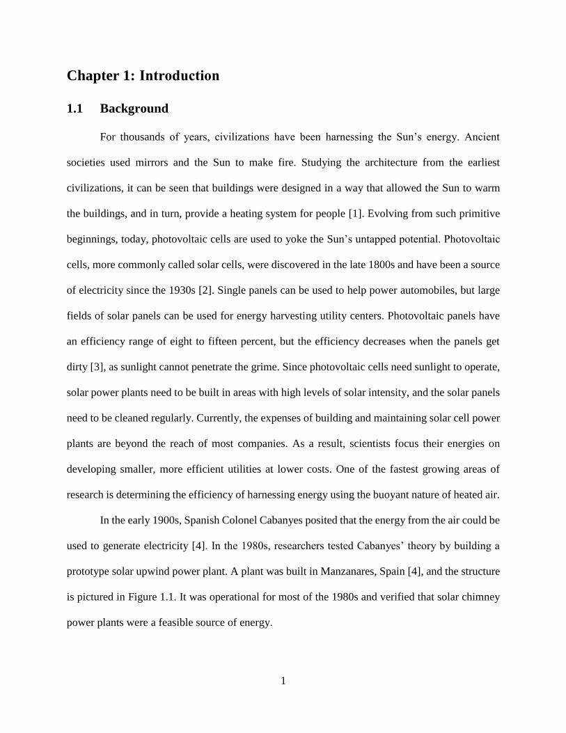
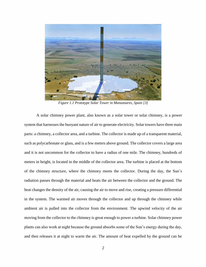
In the early 1900s, Spanish Colonel Cabanyes posited that the energy from the air could be

used to generate electricity [4]. In the 1980s, researchers tested Cabanyes’ theory by building a

prototype solar upwind power plant. A plant was built in Manzanares, Spain [4], and the structure

is pictured in Figure 1.1. It was operational for most of the 1980s and verified that solar chimney

power plants were a feasible source of energy.

2

Figure 1.1 Prototype Solar Tower in Manzanares, Spain [3]

A solar chimney power plant, also known as a solar tower or solar chimney, is a power

system that harnesses the buoyant nature of air to generate electricity. Solar towers have three main

parts: a chimney, a collector area, and a turbine. The collector is made up of a transparent material,

such as polycarbonate or glass, and is a few meters above ground. The collector covers a large area

and it is not uncommon for the collector to have a radius of one mile. The chimney, hundreds of

meters in height, is located in the middle of the collector area. The turbine is placed at the bottom

of the chimney structure, where the chimney meets the collector. During the day, the Sun’s

radiation passes through the material and heats the air between the collector and the ground. The

heat changes the density of the air, causing the air to move and rise, creating a pressure differential

in the system. The warmed air moves through the collector and up through the chimney while

ambient air is pulled into the collector from the environment. The upwind velocity of the air

moving from the collector to the chimney is great enough to power a turbine. Solar chimney power

plants can also work at night because the ground absorbs some of the Sun’s energy during the day,

and then releases it at night to warm the air. The amount of heat expelled by the ground can be

3

increased through the use of underground thermal storage systems [3]. Thermal storage systems

are used to increase the amount of heat transfer to the air by absorbing radiation from the sun. Most

storage systems are made up of materials that have a high heat capacity, such as sealed containers

of water, stored above ground or buried below the surface. Including a layer of gravel on the

ground is another way to augment the amount of heat stored in the ground. Gravel has a high heat

capacity and also allows air to travel through the material and increases heat transfer through

conduction and convection.

Solar upwind power plants are a clean way to harness energy from the sun and to create

electricity [5]. They are also very low maintenance. Because the purpose of the collector is to heat

the air, it is not necessary for the solar tower collector to be kept clean, decreasing the operating

cost, in relation to solar panels requiring frequent cleanings. Solar updraft plants also have a very

unique feature: the area between the collector and the ground can be used as a greenhouse [5]. The

dual functionality of a solar chimney power plant serves two important purposes: generate

electricity and provide agriculture for the surrounding area.

However, solar towers are not used widely because of the high upfront construction costs

necessary for building a large structure and the low energy conversion rate. Solar power plants

only convert one or two percent of the Sun’s potential energy into kinetic energy that can be

harnessed by the turbine [3]. In order to get the most energy out of the chimney system, power

plants with a vast collector area and a soaring chimney are required. The collector size is important

because it is related to the amount of energy the turbine can harvest from the air’s updraft velocity.

One need only consult the theory of conservation of mass to deduce the logic in this concept.

Conservation of mass states that the rate of change of mass exiting a system is equivalent to the

rate of change of mass entering the system. Air entering from under the collector is not moving

4

swiftly, however, the larger the collector, the more air there is entering the system. Therefore, the

velocity of the air exiting at the top of the chimney through a small outlet is directly related to the

amount of air entering the system. The height of the chimney also impacts the amount of air

entering and leaving the solar chimney system. The updraft velocity (𝑣) of the air is related to the

temperature difference (∆𝑇) in the chimney and the height of the chimney (𝐻), and can be derived

from the conservation of energy equation:

𝑣 = √2𝑔𝐻𝛽Δ𝑇 ( 1 )

In Equation ( 1 ), 𝑔 is the Earth’s gravity and 𝑇 is the ambient temperature. The temperature

difference in the chimney is directly impacted by the pressure differential in the chimney structure.

The taller a chimney, the greater the pressure difference between the top and the bottom of the

chimney. The desire for a large collector area and tall tower increases the material costs for the

tower construction. The cost of building materials is astronomical because of the type and quantity

of material needed to structurally support towers that are almost a thousand meters in height [5].

However, once the tower is built, there is very little cost in the upkeep [3].

1.2 Motivation

In recent years, there has been a push to develop third-world countries. An important step

in development is access to energy. The social situation of the impoverished can be improved with

energy because it can be used to help sanitize food and water, and improve living conditions.

Energy can also encourage education because students can study during the day and night.

Economic development can also stem from energy access because it encourages businesses and

manufacturing.

The push to provide universal access to energy has also encouraged the use of renewable

and green energy. Providing energy to the billions of people worldwide using coal and natural gas

5

would greatly reduce the amount fossil fuels available, eventually leading to shortage. Using

renewable resources, such as the sun or wind, would provide almost unconditional access to energy

without depleting the world’s natural resources.

One of the areas that will benefit the most from the push for universal energy is rural Africa.

The majority of Africans do not have access to a reliable source of electricity and many programs

have been created to help energize the area. For instance, President Barack Obama created the

“Power Africa” Initiative to help provide power to the impoverished in sub-Saharan Africa [6].

The initiative teams with the African government to develop green solutions to help solve the

African energy crisis. Ideally these “green solutions” would use the energy harnessed from the

wind, sun, natural gasses, and costal waves to provide power to over twenty-million Africans [6].

One of the most efficient ways to generate energy in Africa is through solar energy because of the

high level of solar radiation.

The average solar radiation in Africa is higher than most other countries. On average,

Africa gets between 6 – 7 kWh/m2 of horizontal irradiation [7]. Horizontal irradiation is another

term for the total radiation: the sum of the direct normal irradiance and diffuse horizontal

irradiance. Figure 1.2 illustrates the high levels of total radiation Africa receives annually.

Research has indicated that smaller towers can be used in environments with higher levels of

radiation [8] because the increase in heat from the Sun causes a greater increase in the air

temperature under the collector. Therefore, the chimney does not have to be as tall to drive the

flow.

6

Figure 1.2 Map of Africa's average annual sum of global horizontal irradiation. SolarGIS © 2014

GeoModel Solar [7]

Installation of a solar chimney power plant would bring electricity and jobs to rural Africa.

During the construction period, the tower would provide jobs to help stimulate the local economy

[8]. After construction finishes, a solar tower would provide electricity for villages at a very low

upkeep cost. The importance of having unconditional, reliable access to electricity is in no small

way exaggerated in helping develop Africa.

1.3 Previous Work

A prototype solar power plant, pictured in Figure 1.1, was built in Manzanares, Spain in

1982 [3]. The plant was built based on the recommendations by Haaf et al. [9], who did an in-

depth analysis on the chimney system to optimize the cost and power output prior to construction.

Environmental factors, including soil characteristics and the Sun’s irradiation, were taken into

account in the energy balances performed on the ground and solar collector. Through extensive

research, Haaf et al. determined that the materials, ground storage, and size of the plant impacted

7

the efficacy of the solar chimney. Using these findings, the chimney in Spain was constructed to

have a height of 200 meters and a diameter of ten meters. The collector, two meters in height,

radiated out from the chimney and had a radius of 120 meters [10]. The first data was collected

within months of the operation’s start. Throughout the study, Haaf [11] monitored the

environmental acting on the structure factors impacted the efficiency of the plant. Furthermore,

the research indicated that large winds and changing ground temperature impacted the movement

of air through the chimney. Despite the small amount of data acquired over a few months, Haaf

[11] was confident that the Manzanares power plant was a success and encouraged the research

and development of solar chimneys. The power plant remained operational for most of the 1980’s

and had a maximum power output of 50 kW [3]. The data collected from the plant is still used

today to validate computational fluid dynamic (CFD) models of solar chimney power plants.

Although the solar chimney was constructed in the 1980s, most research on the subject has

been done since the early 2000s. One of the first CFD models of a solar chimney power plant was

conducted in 2004 by Pastohr et al. [12]. FLUENT was used to create an axisymmetric solar

chimney modeled using the Spanish power plant and included two meters of ground thermal

storage. Pastohr et al. [12] did not include a radiation model; instead, the authors believed that the

radiation from the sun could be modeled as a heat source in a thin layer at the top of the ground.

After simulating different levels of solar irradiation, it was concluded that the more energy in the

system the higher the velocity of the air moving through the chimney. Pastohr et al. [12] also

formulated (and solved) mathematical models based on energy balances on the ground and the

collector. Comparing the FLUENT results to the mathematical results led the authors to the

conclusion that a time-dependent simulation needed to be conducted in order for FLUENT to

properly calculate the heat transfer from the ground to the air.

8

Xu et al. [13] also created an axisymmetric FLUENT model based on the plant in

Manzanares. Using the precedent set by Pastohr et al. [12], a thin heat source was used to model

the radiation of the sun. The main difference between the approaches of these two authors was the

way the thermal storage was modeled. Pastohr et al. [12] treated the thermal storage as a solid

material, while Xu et al. [13] considered the material porous. Xu et al. [13] also included a turbine

in his simulation; the turbine was modeled as a pressure drop at the junction between the collector

and the chimney. The magnitude of the pressure drop was determined by the theoretical turbine

efficiency and power output of the turbine. Xu et al. [13] concluded that energy loss in the system

and power output of the turbine are both directly related to the amount of solar radiation and the

turbine’s efficiency.

The use of porous material in CFD simulations of a thermal storage layer was first studied

by Ming et al. [14]. A solid material only considers conductive heat transfer; however, there is

convective, radiative, and conductive heat transfer in a porous media. Comparing different

mediums for thermal storage, Ming et al. [14] found that materials, such as gravel, with a higher

thermal conductivity are better suited for a thermal storage layer because a higher ratio of the heat

was stored during the day. A study was carried out to determine how the solar radiation impacts

the static pressure, velocity magnitude, and the temperatures of the outlet and energy storage layer.

It was found that the temperatures and velocity increased with a radiation increase while the

pressure decreased. The study help gain an understanding on how the Sun’s energy powered a

solar chimney and impacted the material properties of the air.

In the previous studies discussed, researchers did not include a radiation model to calculate

the fluid properties in a solar chimney power plant. Guo et al. [15] performed simulations to

determine if a radiation model was necessary to correctly model a solar chimney. It was concluded

9

that the temperature in a chimney system was greater without incorporating a radiation model

because the energy losses in the system were not calculated correctly. Guo et al. [15] concluded

that the temperature differences between using and not using a radiation model were significant

enough that it is necessary to incorporate radiation. After deciding it was necessary to use a

radiation model while simulating a solar chimney, the authors went on to study how the magnitude

of solar radiation, the turbine pressure drop, and the ambient temperature impacted the system.

Guo et al. [15] found that the temperature in the chimney increases when either the solar radiation

increased or the pressure drop is increased; however, the updraft velocity decreases with an

increase in pressure drop. Finally, the authors determined that the ambient temperature had a

negligible impact on the system.

A radiation model and the inclusion of a thermal storage system is necessary to develop

and accurately model the greenhouse effect in a solar chimney. The greenhouse effect is when the

ground absorbs some of the sun’s energy and re-radiates it back into the system. The release of

heat from the ground is important to keeping air circulating in a solar chimney at night.

Gholamalizadeh et al. [16] used the Discrete Ordinates radiation model in FLUENT to simulate

the greenhouse effect in a three-dimensional chimney. The authors alter the amount of irradiation

focused on the collector and studied how it impacted the temperature and the velocity in the

chimney system. It was found that increasing the solar irradiation increased the velocity and

temperature in the system. By comparing temperature profiles to other authors (e.g., [12, 14] ),

Gholamalizadeh et al. [16] found that incorporating the greenhouse method greatly altered the

profile in the chimney. Therefore, it is necessary to incorporate the greenhouse method in modeling

a solar chimney power plant to accurately model the heat transfer in the system.

10

As would be expected, the size of a solar chimney greatly influences the efficiency of the

system. Most researchers model their chimneys using the dimensions of the original plant in

Manzanares, Spain. Fasel et al. [17] modeled different sizes of solar chimneys to study how the

efficiency was impacted by the size. The different models were all scaled based on the Manzanares

power plant and the same boundary conditions and solution methods were used in each simulation.

The scale of the model directly impacted the Reynolds number and the systems power. Larger

systems allow for a greater amount of air through the system which increases the temperature and

velocity throughout the system. After the initial study, Fasel et al. [17] created their own

computational code to model a three-dimensional tower. The new code found instabilities that

existed in the flow which could greatly impact the efficiency of the system.

Natural convection is a main source of heat transfer in a solar chimney power plant.

Chergui et al. [18] created a symmetric chimney with no turbine or thermal storage to determine

how air moves in a chimney only incorporating natural convection. The convection was induced

by setting constant temperature boundaries on the chimney walls. The temperature difference in

the chimney was calculated based on the Rayleigh number. The hot temperature was applied to

the ground boundary and a low temperature was specified on the collector wall. The chimney

boundary was considered adiabatic. It was found that increasing the Rayleigh number increased

the airflow through the chimney. Also, the flow started transitioning from laminar to turbulent in

simulations with large Rayleigh numbers. Chergui et al. [18] found turbulence did not fully

develop until the Rayleigh number was greater than 108. Tahar et al. [19] expanded on Chergui et

al.’s [18] experiment by changing the inlet boundary condition and the shape of the chimney. Tahar

et al. [19] also considered the boundary condition of the chimney wall to be the low temperature

11

in the system. The same conclusions were made by both authors, except Tahar et al. [19] found

that turbulence began with Rayleigh numbers as low as 105.

Creating an accurate model of a solar chimney power plant using CFD is an important step

toward the development of more plants. It has been determined that including a radiation model is

important to calculate realistic heat losses in the plant system [15]. Also, it is important to model

the system transiently and with a thermal storage layer to most accurately calculate the heat transfer

in the ground and with the air. It was found that a porous medium is best for the thermal storage

because convective, conductive, and radiative heat transfer are taken into account [14]. Despite

the different models, many of the same conclusions about air flow in a chimney have been reached.

There is a clear connection between the amount of solar irradiation on a plant and the temperature

and velocity of the air moving through the chimney system [13, 14, 15, 16, 17]. It was also found

that the turbine pressure impacted the airflow in the system. When there was greater the pressure

drop and the less efficient the turbine, the velocity magnitude in the chimney system was lower

[13, 15]. While researchers have come a long way in understanding the mechanics of a solar

chimney power plant thirty-two years, the solar chimney continues to be a challenge to model.

Despite number trials and research studies that have been done, an accurate CFD model still

remains elusive to researchers.

1.4 Objectives

The purpose of this thesis is to study of airflow through a solar chimney power plant using

the CFD software FLUENT. It will be assumed that the chimney is located in sub-Saharan and is

operational twenty-four hours a day. The study focuses on modeling the night-time operation of

the solar chimney and assumes no solar irradiation on the system.

12

An axisymmetric solar chimney with a height of 20 m is used to determine the boundary

conditions to best account for the heat transfer occurring between the chimney’s surfaces and the

air moving through the system. Incorporating a layer of thermal storage in the ground is required

to accurately model the chimney system and greatly impacts the airflow. The thermal storage

dissipates heats throughout the night, transferring heat from the ground into the air. Forced-

advection wells can also be incorporated into solar chimney systems to increase the air

temperature. The wells are located in the thermal storage and transfers the heat from the ground

into the airstream.

In order for a solar chimney to be efficient, an extremely tall structure is required. However,

tall chimneys are expensive to build. In sub-Saharan Africa, a tall structure will be an eye-sore in

small villages. To reduce the total height of the chimney structure, chimney clusters are explored.

A cluster consists of either four or five chimneys with a total combined chimney height of 20 m.

The purpose of the clusters is to study the total airflow through the chimney system and compare

to results using a single axisymmetric chimney structure.

This thesis narrates the process used to study a solar chimney. Chapter 2 will discuss the

numerical models and solution methods employed by FLUENT. Chapter 3 contains a grid

resolution study and a validation of the models used employed in FLUENT to simulate a solar

chimney. Chapter 4 examines the heat transfer through the chimney boundaries and investigates

different boundary conditions. Chapter 5 considers airflow through different chimney geometries,

including chimney clusters and chimneys with passive advection wells. Chapter 6 will present the

conclusions of the current study and provide recommendations for future work.

13

Chapter 2: Numerical Approach

The following will discuss the equations and models incorporated by FLUENT to model a

solar chimney power plant with thermal storage. The governing equations will be presented in two

forms: the original derivative form and in a non-dimensional form. Then, the models for

turbulence, radiation, and porous materials will be explored. Finally, the discretization methods

used will be examined.

2.1 Governing Equations

FLUENT employs the fundamental three-dimensional fluid mechanic equations for

conservation of mass, momentum, and energy to calculate fluid properties. The conservation of

mass equation, known also as the continuity equation, is:

𝜕𝜌

𝜕𝑡+ ∇⃗⃗⃗ ∙ (𝜌�⃗�) = 0 ( 2 )

where 𝑡 represents time, 𝜌 is density, and �⃗� is the velocity vector.

The equation for conservation of momentum can be expressed as:

𝜕

𝜕𝑡(𝜌�⃗�) + ∇⃗⃗⃗ ∙ (𝜌�⃗��⃗�) = −∇⃗⃗⃗𝑝 + ∇⃗⃗⃗ ∙ (𝜏̿) + 𝜌�⃗� ( 3 )

where 𝑝 is the static pressure. The stress tensor, 𝜏̿, is expressed as:

𝜏̿ = 𝜇 [(∇⃗⃗⃗�⃗� + ∇⃗⃗⃗�⃗�𝑇) −2

3∇⃗⃗⃗ ∙ �⃗�𝐼] ( 4 )

where I is the identity matrix and 𝜇 is the dynamic viscosity. The final term in the momentum

equation represents the buoyancy force.

The energy equation is:

𝜕

𝜕𝑡(𝜌𝐸) + ∇⃗⃗⃗ ∙ (�⃗�(𝜌𝐸 + 𝑝)) = ∇⃗⃗⃗ ∙ 𝑘∇⃗⃗⃗𝑇 + ∇⃗⃗⃗ ∙ (𝜏̿ ∙ �⃗�) + 𝑆ℎ ( 5 )

14

where E is the total of the potential, kinetic, and internal energy in the system. The internal energy,

ℎ, is the enthalpy of the fluid and is expressed as:

ℎ = ∫ 𝑐𝑝𝑑𝑇

𝑇

𝑇0

( 6 )

where 𝑐𝑝 is the constant pressure specific heat. The total conductivity, 𝑘𝑒𝑓𝑓, takes into account

the thermal conductivity of the fluid and the turbulent thermal conductivity. The final term in

Equation ( 5 ) , Sh, is an additional energy source term.

There are multiple assumptions that can be adapted into the governing equations. First, the

Boussinesq model can be assumed for the buoyancy force in the momentum equation. The

Boussinesq buoyancy model assumes that the density is only a function of temperature, and can

be expressed in terms of the thermal expansion coefficient, 𝛽:

𝛽 = −1

𝜌(

𝜕𝜌

𝜕𝑇)

𝑝 ( 7 )

Equation ( 7 ) relates how the density of the fluid changes with temperature. Due to the small

temperature change in the chimney system, the density can be expressed as:

(𝜌 − 𝜌0) ≈ −𝜌0𝛽(𝑇 − 𝑇0) ( 8 )

where the subscript 0 indicates a reference value. Implementing the Boussinesq model, FLUENT

only uses Equation ( 8 ) to calculate the density associated with the buoyancy force in the

momentum equation. The density in the continuity equation, the energy equation, and the left-hand

side of the momentum equation can be expressed as the reference density, 𝜌0. Assuming an

incompressible fluid, the continuity equation can be simplified to:

∇⃗⃗⃗ ∙ �⃗� = 0 ( 9 )

Incorporating incompressible flow, the stress tensor Equation ( 4 ) can be reduced to:

15

𝜏̿ = 𝜇∇⃗⃗⃗�⃗� ( 10 )

The above assumptions allow for the viscous heating term, ∇ ∙ (τ̿ ∙ v⃗⃗), in the energy equation,

Equation ( 5 ), to be neglected. Since the energy source term is not needed in every thermodynamic

case, it can also be disregarded. Implementing all of the above simplifications and dividing the

momentum equation by 𝜌0, the momentum and energy equations become:

𝜕�⃗�

𝜕𝑡+ �⃗�∇⃗⃗⃗ ∙ �⃗� = −

1

𝜌0∇⃗⃗⃗𝑝 +

𝜇

𝜌0∇⃗⃗⃗2�⃗� + �⃗�[1 − 𝛽(𝑇 − 𝑇0)] ( 11 )

𝜕𝑇

𝜕𝑡+ �⃗� ∙ ∇⃗⃗⃗𝑇 = 𝛼∇⃗⃗⃗2𝑇 ( 12 )

where 𝛼 = 𝑘/𝜌𝑐𝑝.

2.2 Non-Dimensional Analysis

A non-dimensional analysis was performed on the governing equation to show the

importance of each term. Dimensionless variables were created using the variables 𝜌0, 𝐿, and 𝑢0.

The non-dimensional variables formed are indicated with the superscript * and are shown below.

𝑡∗ = 𝑡𝑢0

𝐿 ( 13 )

∇⃗⃗⃗∗= ∇⃗⃗⃗𝐿 ( 14 )

�⃗�∗ =

�⃗�

𝑢0 ( 15 )

𝑝∗ =𝑝

𝜌0𝑢02 ( 16 )

g⃗⃗∗ = g⃗⃗

𝐿

𝑢02 ( 17 )

𝜃∗ =

𝑇 − 𝑇0

𝑇𝐻 − 𝑇0 ( 18 )

Substituting the above variables into Equations ( 11 ) and ( 12 ), the following non-dimensional

equations are formed:

16

∇⃗⃗⃗∗ ∙ �⃗�∗ = 0 ( 19 )

𝜕�⃗�∗

𝜕𝑡∗+ �⃗�∗∇⃗⃗⃗∗ ∙ �⃗�∗ = −∇⃗⃗⃗∗𝑝∗ +

1

𝑅𝑒∇⃗⃗⃗∗

2�⃗�∗ −

𝐺𝑟

𝑅𝑒2𝜃∗ + g⃗⃗∗ ( 20 )

𝜕𝜃∗

𝜕𝑡∗+ �⃗�∗ ∙ ∇⃗⃗⃗∗𝜃∗ =

1

𝑅𝑒𝑃𝑟∇⃗⃗⃗∗

2𝜃∗ ( 21 )

In Equations ( 20 ) and ( 21 ), 𝑅𝑒 represents the Reynolds number given by:

𝑅𝑒 =𝜌𝑢0𝐿

𝜇 ( 22 )

where 𝜇 is the dynamic viscosity. The Reynolds number is the ratio of momentum forces to viscous

forces. The Grashof, 𝐺𝑟, number also appears in Equation ( 20 ), and is given by:

𝐺𝑟 =�⃗�𝛽(𝑇𝐻 − 𝑇0)𝐿3

𝜈2 ( 23 )

The Grashof number is the ratio of buoyancy forces to viscous forces. Finally, the Prandtl number

appears in the non-dimensional energy equation and is expressed as the ratio of momentum to

thermal diffusivities

𝑃𝑟 =𝜈

𝛼 ( 24 )

Another important dimensionless variable that does not appear in the governing equations

is the Rayleigh number. The Rayleigh number is the product of the Grashof and Prandtl numbers

and is:

𝑅𝑎 =�⃗�𝛽(𝑇𝐻 − 𝑇0)𝐿3

𝜈𝛼 ( 25 )

2.3 Turbulence Modelling

The realizable 𝑘 − 𝜀 turbulence model was used throughout the study. The 𝑘 − 𝜀

turbulence model assumes that the flow is fully turbulent and the effects of molecular viscosity

can be neglected. The realizable model was chosen because the dissipation rate, 𝜀, is calculated

using a derivation of the mean-square vorticity fluctuation equation [20]. The realizable 𝑘 − 𝜀

17

model employs two equations to calculate the turbulent kinetic energy, 𝑘, and the dissipation rate,

where:

𝜕

𝜕𝑡(𝜌𝑘) + ∇⃗⃗⃗ ∙ (𝜌𝑘�⃗�) = ∇⃗⃗⃗ ∙ [(𝜇 +

𝜇𝑡

𝜎𝑘) �⃗⃗�] + 𝐺𝑘 + 𝐺𝑏 − 𝜌𝜀 ( 26 )

𝜕

𝜕𝑡(𝜌𝜀) + ∇⃗⃗⃗ ∙ (𝜌𝜀�⃗�)

= ∇⃗⃗⃗ ∙ [(𝜇 +𝜇𝑡

𝜎𝜀) 𝜀] + 𝜌𝐶1𝑆𝜀 − 𝜌𝐶2

𝜀2

𝑘 + √𝜈𝜀+ 𝐶1𝜀

𝜀

𝑘𝐶3𝜀𝐺𝑏

( 27 )

The variable, 𝐶1, is determined using the following relation:

𝐶1 = max [0.43,𝑆

𝑘𝜀

𝑆𝑘𝜀 + 5

] ( 28 )

In Equation ( 26 ), 𝐺𝑘 is the production of turbulent kinetic energy due to velocity gradients and

can be calculated using the following equation:

𝐺𝑘 = 𝜇𝑡𝑆2 ( 29 )

The production of turbulent kinetic energy due to buoyancy, 𝐺𝑏 in the 𝑘 − 𝜀 equations is calculated

by:

𝐺𝑏 = 𝛽�⃗�𝜇𝑡

𝑃𝑟∇⃗⃗⃗𝑇 ( 30 )

The eddy viscosity, 𝜇𝑡, can be calculated using the following equation:

𝜇𝑡 = 𝜌𝐶𝜇

𝑘2

𝜀 ( 31 )

The variable 𝐶𝜇 is based on the mean rate of strain and rotation, the angular velocity, and the

system rotation. In Equation ( 27 ), 𝐶2 and 𝐶1𝜀 are constants with values 1.9 and 1.44, respectively.

In the realizable 𝑘 − 𝜀 model, the turbulent Prandtl numbers for turbulent kinetic energy (𝜎𝑘) and

dissipation rate (𝜎𝜀) are 1.0 and 1.3, respectively. The values have been determined from

18

experiments on turbulent flow. The amount that the diffusion rate is impacted by buoyancy is given

in the term 𝐶3𝜀:

𝐶3𝜀 = tanh |𝜈

𝑢| ( 32 )

2.4 Radiation Modelling

In order to correctly account for radiative heat transfer in the solar chimney simulation, a

radiation model is employed. There are five different radiation models offered in FLUENT, but

only one model that takes into account the transparency of a material. The Discrete Ordinates (DO)

model was chosen because of the transparent nature of the solar collector. The DO model calculates

the amount of radiation reflected, absorbed, and emitted from incident radiation occurring on a

surface. The DO model calculates how much energy is absorbed, reflected, and transmitted

through a material using the radiative transfer equation:

𝑑𝐼(�̅�, �̅�)

𝑑𝑠+ (𝑎 + 𝜎𝑠)𝐼(�̅�, �̅�) = 𝑎𝑛2

𝜎𝑇4

𝜋+

𝜎𝑠

4𝜋∫ 𝐼(�̅�, �̅�′)𝜙(�̅� ∙ �̅�′)𝑑𝛺′

4𝜋

0

( 33 )

where 𝐼(�̅�, �̅�) is the radiation intensity based on the position and direction, 𝑎 is the absorption

coefficient, 𝑛 is the refractive index, 𝜎𝑠 is the scattering coefficient, and 𝜎 is the Stefan-Boltmann

constant.

When the DO model is used, additional properties need to be specified for the materials

used. The refractive index needs to be specified for materials identified as semi-transparent

materials. The absorption coefficient and scattering coefficient also need to be specified. The

absorption coefficient, 𝑎, can be calculated using the equation:

𝐼 = 𝐼0𝑒−𝑎𝑥 ( 34 )

where 𝐼 is the radiation intensity and 𝑥 is the distance through the material in centimenters.

19

The DO model also accounts for the external irradition flux on semi-transparent surfaces.

For modeling a solar chimney during the night, the external flux is the night-sky radiation on the

collector. The ground boundary is treated as a gray-body because it is not transparent. The DO

model calculates the amount of energy reflected, absorbed, and the emission from the ground.

2.5 Formulation of Porous Materials

The top layer of the ground acts as thermal storage. The ground absorbs some of the Sun’s

radiation and then releases back into the air during the night. It is important to correctly model the

ground in FLUENT so that conductive, convective, and radiative heat transfer are all taken into

account. When modeling a solid zone, FLUENT only calculates the heat transfer due to

conduction, therefore, the ground has to be considered a packed-bed porous medium. FLUENT

calculates heat transfer from convection, radiation, and conduction in a porous zone. The packed

bed model was chosen to model the ground because common ground materials, such as dirt, gravel,

or sand, are made up of millions of particles. The packed-bed model accounts for the air moving

between and interacting with the dirt particles [21].

Incorporating the porous model into the simulation adds an additional source term, 𝑆𝑖, to

the momentum equation.

𝑆 = − (

𝜇

𝛼�⃗� + 𝐶2

1

2𝜌|�⃗�|�⃗� ) ( 35 )

where 1 𝛼⁄ and 𝐶2 represent the viscous resistance and inertial losses, respectively, through a

homogeneous porous medium. The viscous resistance can be described as the inverse of the

permeability, 𝛼. For a packed bed, the permeability can be calculated as:

𝛼 =

𝐷𝑝2

150

𝜀3

(1 − 𝜀)2 ( 36 )

20

where 𝐷𝑝 is the particle diameter of the soil and 𝜀 is the void fraction. The void fraction is defined

as the volume of a void space in a region divided by the total volume. The inertial losses in the

medium can be calculated using the equation:

𝐶2 =

3.5

𝐷𝑝 (1 − 𝜀)

𝜀 ( 37 )

The porous model modifies the standard energy equation, Equation ( 3 ), to account for the

different mediums. Equation ( 3 ) becomes:

𝜕

𝜕𝑡(𝛾𝜌𝑓𝐸𝑓 + (1 − 𝛾)𝜌𝑠𝐸𝑠) + ∇⃗⃗⃗ ∙ (�⃗�(𝜌𝑓𝐸𝑓 + 𝑝))

= 𝑆𝑓ℎ + ∇⃗⃗⃗ ∙ [𝑘𝑒𝑓𝑓 ∇⃗⃗⃗𝑇 − (∑ ℎ𝑖𝐽𝑖

𝑖

) + (𝜏̿ ∙ �⃗�)]

( 38 )

In the above equation, the subscript 𝑓 signifies a fluid property while the subscript 𝑠 indicates a

solid property. The thermal conductivity of the system, 𝑘𝑒𝑓𝑓, is the volume average of the fluid

and solid conductivities, and is calculated by:

𝑘𝑒𝑓𝑓 = 𝛾𝑘𝑓 + (1 − 𝛾)𝑘𝑠 ( 39 )

2.6 Solution Methods

A control-volume discretization is used by FLUENT to solve the governing equations with

a pressure-based solver. FLUENT uses the geometry’s mesh, created in ICEM, to divide the cells

into control volumes and then solves for the velocity, pressure, temperature and other unknown

variables. The pressure and velocity equations are coupled using the semi-implicit method for

pressure linked equations (SIMPLE) algorithm [20]. The SIMPLE algorithms starts by estimating

a pressure using the momentum equation and then corrects the pressure and the velocity until the

continuity equation is solved.

21

The momentum, energy, radiation, and turbulence equations are all solved using a second-

order upwind interpolation. The scheme employs a Taylor-Series expansion about the center of a

cell that uses the values of two cells upwind. The Least Squares Cell-Based evaluation is used for

the spatial discretization of the gradient, and calculates the gradient in the center of control-volume

cell by using the gradients of the four adjacent cells. To solve for the pressure discretization, the

pressure staggering option (PRESTO) scheme was employed [20]. The transient formulation also

used a second-order upwind discretization. The solar chimney power plant is modeled transiently

because the properties of the chimney will change over time.

FLUENT calculates residuals for the governing equations, the turbulence equations, and

the equation for DO-Intensity. The convergence criteria is 10−6 for all residuals, except the

residual for DO-Intensity which is set as 10−5.

22

Chapter 3: Validation

The following chapter reviews the methodology used to successfully model a solar

chimney using FLUENT. The grid resolution study will be discussed. Results from the study will

be used to determine an appropriate mesh size to use in all the simulations. The validation study

will confirm the different models employed by FLUENT are suitable to simulate the airflow

through a solar chimney system.

3.1 Grid Convergence

A grid convergence index (GCI) uses the Richardson Extrapolation to determine the

discretization error associated with the grid spacing [22]. The GCI is used for a grid resolution

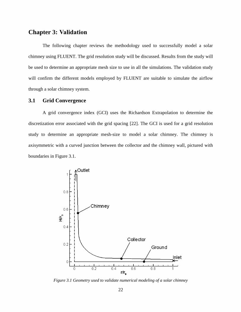
study to determine an appropriate mesh-size to model a solar chimney. The chimney is

axisymmetric with a curved junction between the collector and the chimney wall, pictured with

boundaries in Figure 3.1.

Figure 3.1 Geometry used to validate numerical modeling of a solar chimney

23

The boundary conditions in the GCI are the boundary conditions proposed by Tahar et al.

[19]. A zero-velocity inlet is specified at a temperature of 290 K. The outlet is set to atmospheric

pressure and has an ambient temperature of T0 = 290 K. The collector and chimney walls are

designated as no-slip boundaries and have a constant temperature of 290 K. The ground boundary

is also considered no-slip and has a constant temperature of 290 K. The temperature of the collector

and chimney is calculated using Ra = 106 assuming T0 = TC = 290 K. The temperature field in the

system is initialized at 290 K and the velocity field is initialized to 0 m/s. The flow is considered

to be laminar.

The curved geometry prevented the use of an even grid distribution; however, the spacing

between the nodes is increased or decreased by a factor of two for the different mesh sizes. Four

different mesh sizes are used to complete the GCI. Figure 3.2, is the solar chimney with a coarse

mesh. All the cells in the mesh are quadrilaterals. Two finer meshes and one coarser mesh were

also created. Table 3.1 outlines the differences between all of the mesh sizes. Each mesh is

assigned a number between one and four corresponding to how fine it is, with one being the finest.

Table 3.1 Summary of the mesh information used to calculate the GCI

Coarsest (4) Coarse (3) Medium (2) Fine (1)

Number of Cells 600 2400 9600 38400

Minimum Cell Size [m] 0.06 0.03 0.015 0.0075

Maximum Cell Size [m] 0.434 0.216 0.108 0.054

Spacing along Axis [m] 0.2 0.1 0.05 0.025

24

Figure 3.2 Chimney geometry showing the coarse mesh

The mesh spacing is important when calculating the order of accuracy and the GCI. The grid size,

ℎ, can be expressed as:

ℎ = [1

𝑁∑ ∆𝐴𝑖

𝑁

𝑖=1

]

1/2

( 40 )

where 𝑁 is the total number of cells and ∆𝐴𝑖 is the area of each cell. The grid size is used to

calculate the refinement factor of the mesh. The refinement factor, 𝑟, is the ratio of coarse to fine

mesh size, and in the study conducted, 𝑟 = 2. The order of accuracy, 𝑝, of the system is calculated

using the equation:

𝑝 = |ln |

𝜙3 − 𝜙2

𝜙2 − 𝜙1|

ln(𝑟)| ( 41 )

25

where 𝜙𝑖 is the variable solution on a node point for the designated grid size. The variable that is

analyzed in the study is the axial velocity along the axis of the geometry. The GCI between two

mesh sizes is calculated using the equation:

𝐺𝐶𝐼2→1 =1.25𝑒2→1

𝑟2→1 𝑝 − 1

( 42 )

where 𝑒2→1 is the error for the node value between meshes and is found using:

𝑒2→1 = |𝜙1 − 𝜙2

𝜙1| ( 43 )

The order of accuracy, error, and GCI are calculated at each coincident nodal point along

the entire height of the chimney, and are the nodes in the coarsest mesh being analyzed. The final

values for the order of accuracy, error, and GCI are the average of all the values calculated over

the axis height. Because all of the data points are extremely similar above the point, 𝐻 𝑟0⁄ = 0.35,

the final averages are done twice: once incorporating the entire length of the axis and a second

time focusing on the portion below and including 𝐻 𝑟0⁄ = 0.35. GCI calculations are performed

for two different sets of meshes: once using the three coarsest meshes and a second time using the

three finest meshes. As expected, there was less error comparing the three finer meshes. The final

calculated values for the order of accuracy, the error, and the GCI are detailed in Table 3.2.

Table 3.2 Final values for axial velocity and the corresponding error in the GCI study

Meshes 4, 3, and 2 Meshes 3, 2, and 1

All Data 𝟎 <𝑯

𝒓𝟎≤ 𝟎. 𝟑𝟓 All Data 𝟎 <

𝑯

𝒓𝟎≤ 𝟎. 𝟑𝟓

𝒑 1.692 2.689 5.605 2.398

𝒆𝟒→𝟑(%) 146.0 85.4 - -

𝒆𝟑→𝟐(%) 2151.0 17.0 2173.3 19.45

𝒆𝟐→𝟏(%) - - 10.66 6.17

𝑮𝑪𝑰𝟒→𝟑 (%) 176.9 19.8 - -

𝑮𝑪𝑰𝟑→𝟐(%) 3192.0 5.65 14.89 7.63

𝑮𝑪𝑰𝟐→𝟏(%) - - 1.125 2.66

26

A comparison of the velocity values associated with the mesh sizes is illustrated in Figure

3.3. One can observe that the maximum velocity along the axis of symmetry decreases as the mesh

size becomes finer. Also, the difference in velocity values decrease as the mesh becomes finer.

Figure 3.3 only captures axial-velocity profile for 𝐻 𝑟0⁄ between zero and 0.4 because all the data

points above that are shown in a figure as coincindent because of the neligible difference in

velocity values.

Figure 3.3 Axial velocity profiles at node points along the axis of the chimney for four different grid

resolutions

From the grid-size study, it can be concluded that the medium mesh is a sufficient spacing

to use in modeling a solar chimney. In situations where there is large geometric configurations to

be run, the coarse mesh is sufficient to calculate the flow fields.

27

3.2 Validation

Tahar et al. [19] simulated natural convection in a solar chimney to study how the Rayleigh

number impacted airflow through a chimney. Multiple Rayleigh numbers and two different

chimney geometries are used to study how the Rayleigh number and the chimney geometry impact

the temperature and velocity fields. The flow is driven by a temperature difference in the system

created by specifying low and high temperatures on the upper and lower walls of the system,

respectively. The temperature difference was calculated using the Rayleigh number of the system,

and the temperature variation increases with increasing Rayleigh numbers. Other boundary

conditions include a zero-velocity inlet at 290 K, an outlet specified at atmospheric pressure and

290 K, and a rotational axis of symmetry. The authors reached the conclusion that higher Rayleigh

numbers induce turbulence and increase the temperature in the chimney.

The results from Tahar et al. [19] paper are used to validate the methods used in FLUENT

to model a solar chimney. Using a geometry similar to Tahar et al. [19], shown in Figure 3.1, the

Rayleigh numbers are used to find the wall temperature which are the wall’s boundary conditions

in the system. The geometry has a length of 1 m, which is the characteristic length used in

calculating the Rayleigh number in the comparison. The temperature and axial velocity will be

compared to the data of Tahar et al. [19] for two of the Rayleigh numbers analyzed. In the

comparison, only the most informative portion of the geometry will be shown: the curved junction

of the chimney, enlarged in Figure 3.4. The figure illustrates that the most revealing portion of the

axial velocity contours occurs at the center of the geometry. The center junction is also the most

revealing portion of the geometry for the temperature contours.

28

Figure 3.4 Emphasis on the center of the geometry showing the most informative contour of the axial

velocity

Tahar et al. [19] analyzed the flow based on three different Rayleigh numbers. The

Rayleigh numbers used are: 103, 104, and 105. The results obtained from the two lower Rayleigh

numbers are extremely similar so only Ra = 103 and Ra = 105 are used in the validation study. The

Rayleigh number and Reynolds number are calculated at three different locations in the geometry,

h1, h2, and L, which are shown in Figure 3.5. The height, h1, indicates the inlet height; h2 is the

height at the center of the curve. The length of the collector, L, and the height of the chimney, H,

are the same, so only one Rayleigh number is calculated for those values.

29

Figure 3.5 Validation geometry with dimensions.

Different authors have calculated the Rayleigh number in a solar chimney using different

values. Chergui et al. [18] used the height of a collector without a curve, while Ming et al. [14]

uses the length of the collector. However, Tahar et al. [19] did not specify the characteristic length

used in the calculations. The Rayleigh and Reynolds numbers were calculated using different

characteristic lengths in the chimney system and the corresponding values are listed in Table 3.3.

The Reynolds number is calculated using the velocity equation presented in Equation ( 1 ), which

bases the velocity on the characteristic lengths. Using the characteristic lengths of h1 and h2, the

Reynolds and Rayleigh numbers represent pipe flow in the system. For pipe flow, the transitional

Reynolds number is 3,000 [20]. However, using the characteristic length L represents flow over a

flat plate, where the transitional Reynolds number is 5 × 105 and the transitional Rayleigh number

is 109 [20]. In the validation, the length of the collector, L, will be used.

30

Table 3.3 Rayleigh and Reynolds Numbers based on different characteristic lengths in the validation

geometry

Ra (L) Ra (h1) Ra (h2) Re (L) Re (h1) Re (h2)

103 0.01563 1.953 29.9 0.118 1.32

105 1.563 195.3 299 1.18 13.2

108 1563 195300 9460 37.4 418

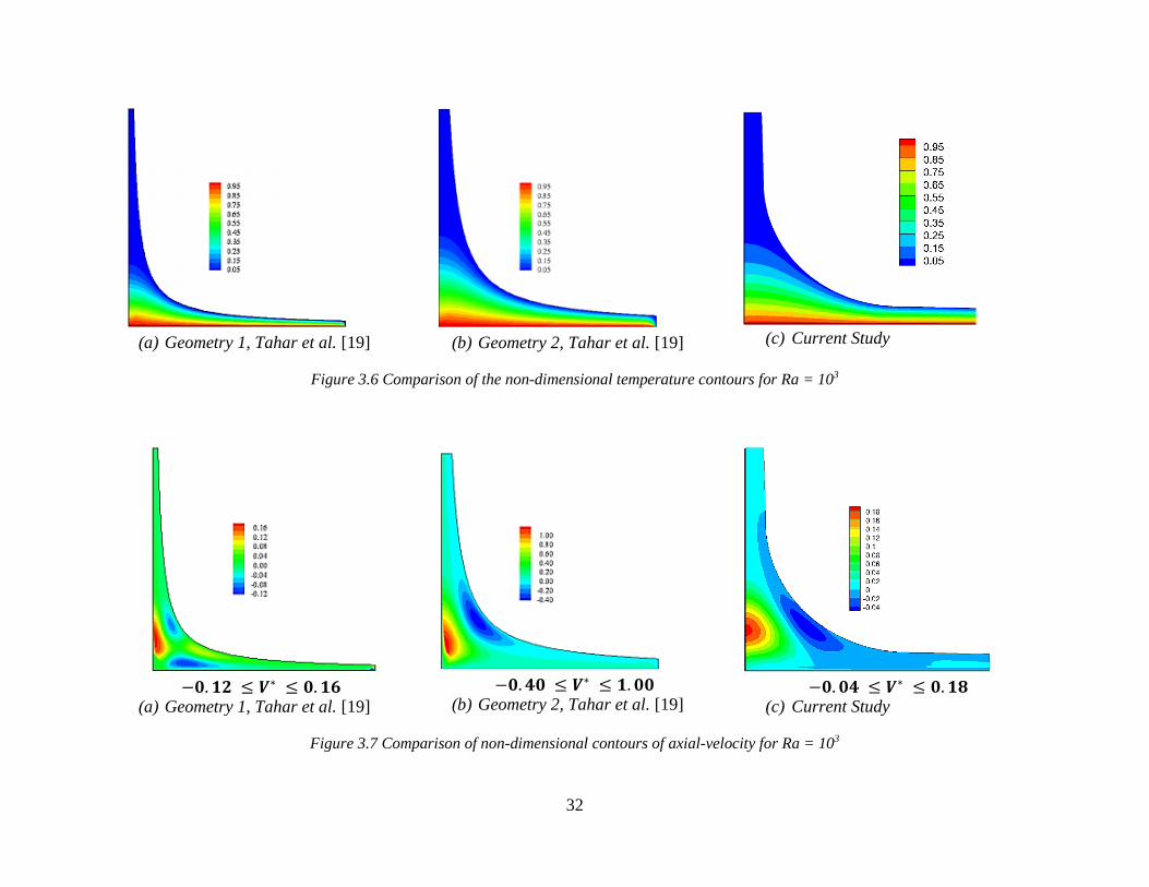
The results from Tahar et al. [19] for Ra = 103 depict smooth temperature contours

throughout the chimney, and the study produced similar contours. The temperature contours are

non-dimensionalized using Equation ( 18 ) assuming the temperature that is specified on the cold

wall and at the inlet is considered the reference temperature, 𝑇0. Figure 3.6(a) and (b) present the

two geometries used in Tahar et al. [19]. Geometry 1 has a smaller curve and there is a shorter

distance between the two walls than Geometry 2. However, the temperature contours look similar

despite the geometric differences. Figure 3.6(c) is the geometry created in this work showing the

temperature contour.

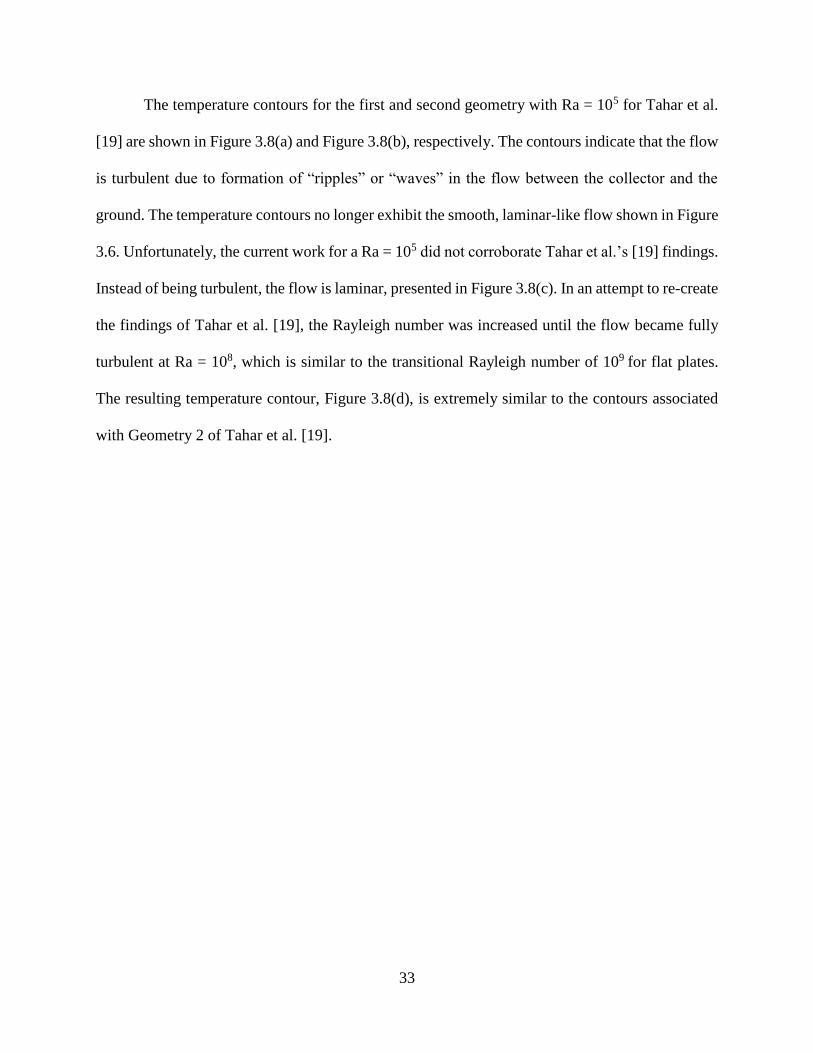
The contours of non-dimensional axial velocity are also used to study the effects of the

Rayleigh number. The equation to non-dimensionalize the velocity, taken from a similar study on

natural convection by Chergui et al. [18], is:

𝑉∗ =

𝑉

√𝑔𝛽𝐿∆𝑇 ( 44 )

The non-dimensional velocity, 𝑉∗ , is computed by dividing the velocity field in the chimney

system by the velocity relationship presented in Equation ( 1 ). The characteristic length used is

the length of the collector, which is also the characteristic length in calculating the Rayleigh

number. The resulting non-dimensionalized velocity is extremely small, so 𝑉∗ has been increased

by a factor of 100. Comparing the results from the current study to the first and second geometry

31

from Tahar et al. [19] in Figure 3.7, it is seen that the re-created contours are extremely similar to

Geometry 2.

32

(a) Geometry 1, Tahar et al. [19]

(b) Geometry 2, Tahar et al. [19]

(c) Current Study

Figure 3.6 Comparison of the non-dimensional temperature contours for Ra = 103

−𝟎. 𝟏𝟐 ≤ 𝑽∗ ≤ 𝟎. 𝟏𝟔 (a) Geometry 1, Tahar et al. [19]

−𝟎. 𝟒𝟎 ≤ 𝑽∗ ≤ 𝟏. 𝟎𝟎

(b) Geometry 2, Tahar et al. [19]

−𝟎. 𝟎𝟒 ≤ 𝑽∗ ≤ 𝟎. 𝟏𝟖

(c) Current Study

Figure 3.7 Comparison of non-dimensional contours of axial-velocity for Ra = 103

33

The temperature contours for the first and second geometry with Ra = 105 for Tahar et al.

[19] are shown in Figure 3.8(a) and Figure 3.8(b), respectively. The contours indicate that the flow

is turbulent due to formation of “ripples” or “waves” in the flow between the collector and the

ground. The temperature contours no longer exhibit the smooth, laminar-like flow shown in Figure

3.6. Unfortunately, the current work for a Ra = 105 did not corroborate Tahar et al.’s [19] findings.

Instead of being turbulent, the flow is laminar, presented in Figure 3.8(c). In an attempt to re-create

the findings of Tahar et al. [19], the Rayleigh number was increased until the flow became fully

turbulent at Ra = 108, which is similar to the transitional Rayleigh number of 109 for flat plates.

The resulting temperature contour, Figure 3.8(d), is extremely similar to the contours associated

with Geometry 2 of Tahar et al. [19].

34

Ra = 105

(a) Geometry 1, Tahar et al. [19]

Ra = 105

(b) Geometry 2, Tahar et al. [19]

Ra = 105

(c) Current Study

Ra = 108

(d) Current Study

Figure 3.8 Comparison non-dimensional temperature contours for Ra = 105 and Ra = 108

35

The same incongruence can be seen analyzing the contours of the axial velocity from Tahar

et al. [19] produced for a Ra = 105. Geometries 1 and 2, Figure 3.9(a) and (b), respectively, indicate

a turbulent flow at a Rayleigh number of 105. However, a laminar flow is seen in the current work,

shown in Figure 3.9(c) with the same Rayleigh number. Velocity contours for Ra = 108 depict a

turbulent flow in Figure 3.9(d) and are more similar to Geometry 1.

−𝟐𝟎. 𝟎𝟎 ≤ 𝑽∗ ≤ 𝟑𝟎. 𝟎𝟎

Ra = 105

(a) Geometry 1, Tahar et al. [19]

−𝟑𝟎. 𝟎𝟎 ≤ 𝑽∗ ≤ 𝟐𝟓. 𝟎𝟎

Ra = 105

(b) Geometry 2, Tahar et al. [19]

−𝟎. 𝟒𝟎 ≤ 𝑽∗ ≤ 𝟐. 𝟎𝟒

Ra = 105

(c) Current Study

−𝟓. 𝟑𝟒 ≤ 𝑽∗ ≤ 𝟐𝟎. 𝟏𝟎

Ra = 108

(d) Current Study

Figure 3.9 Comparison of non-dimensional axial-velocity contours associated with Ra = 105 and Ra =

108

36

One of the main sources of discrepancies between the contours is the geometry. Tahar et

al. [19] used two geometries with very pronounced curves. However, the angles of curvature are

not specified in the published paper so the exact geometry could not be re-created. Also, the

reference variables Tahar et al. [19] used to perform the non-dimensional analysis are not included

in the paper. The omission of the non-dimensional equations affects the magnitude of the velocity;

however, the shape of the contours are not impacted.

The study by Tahar et al. [19] is extremely similar to a natural convection study by Chergui

et al. [18]. Chergui et al. [18] tested natural convection in a solar chimney with a right-angle

between the chimney structure and the collector. Many of the conclusions reached by Tahar et al.

[19] validate the findings published by Chergui et al. [18]. However, Chergui et al. [18] found that

the flow in a solar chimney becomes turbulent at a Ra = 108, while Tahar et al. [19] found that the

flow became turbulent at Ra = 105. The analysis in this thesis found that the transition to turbulence

for flow in a solar chimney driven by natural convection occurs at a Rayleigh number of 108, which

agrees with the results presented by Chergui et al. [18]. Overall, the validation study is successful,

confirming that the models chosen in FLUENT are appropriate to model a solar chimney.

37

Chapter 4: Exploration of Boundary Conditions

The process used to create appropriate night-time boundary conditions for a solar chimney

is examined. First, the geometries used in the study of boundary conditions will be discussed. An

investigation of the appropriate boundary conditions for the solar collector and ground will follow.

The chapter will conclude with the analysis of the night-time progression of a solar chimney with

a thermal storage layer.

4.1 Geometric Configurations

The solar chimney geometry is a large three-dimensional structure consisting of a tall

chimney and a large collector area. The original solar chimney power plant in Manzanares, Spain

(Figure 1.1) had a height of 200 meters, a collector radius of 120 meters, and a chimney diameter

of 10m. Because of the immense size of the structure, a chimney plant one-tenth the size of the

Manzanares plant is used in the exploration of the correct boundary conditions to model the night-

time operation of a solar chimney. The only change in the chimney geometry is the chimney

diameter which is 0.6 m instead of 1 m. The change was made as a way to increase the outlet

velocity of the system.

Two models of a solar chimney, a three-dimensional model (Figure 4.1) and an

axisymmetric two-dimensional model (Figure 4.2), are created using cylindrical coordinates

system. Specifying an axis of symmetry assumes that there is no circumferential gradient in the

flow. The two-dimensional geometry includes a layer of thermal storage. In many cases, the

thermal storage is neglected and the ground boundary is considered to be at a height of 0 m.

38

Figure 4.1 Three-dimensional model of a solar chimney

Figure 4.2 Two-dimensional axisymmetric model of a solar chimney with thermal storage

39

A validation is performed to verify that the axisymmetric geometry can be used to

accurately model the air flow in the chimney. The thermal storage is neglected and a constant heat

flux of 800 W/m2 is applied to the ground. The outlet is set at atmospheric pressure with a

temperature of 293 K. The inlet is considered a velocity inlet with air entering the system with a

radial velocity of 11 m/s and a temperature of 293 K. The chimney wall is considered adiabatic.

The system is initialized to atmospheric pressure, a temperature of 293 K, and a velocity field of

0 m/s. The solution is forced to steady state and the axisymmetric geometry converged to 10-6. The

three-dimensional geometry converges to 10-3. The temperature and velocity magnitude are

compared along the centerline to determine if the axisymmetric geometry is an effectively way to

model a three-dimensional solar chimney system.

The centerline temperature comparison is shown in Figure 4.3. The shape of the

temperature profile is extremely close together; however, there are some discrepancies between

the approximate heights of 1 m and 5 m. Calculating the error between the two geometries, it is

found that the average error in temperature is 0.08% and the maximum temperature error is 0.85%.

The magnitude of the velocity is also compared along the centerline. Observing the profiles

in Figure 4.4, both the shape and the magnitude are in excellent agreement between the

axisymmetric and three-dimensional geometries. The average velocity error is calculated to be

0.53% with a maximum error of 7.89%.

40

Figure 4.3 Temperature profile along the centerline of the axisymmetric geometry and three-dimensional

geometry

Figure 4.4 Comparison of the centerline velocity between the two-dimensional axisymmetric geometry

and the three-dimensional geometry

41

There are a few sources that can be attributed to the variable discrepancies between the

geometric profiles. First, there is a very small difference in the inlet and outlet areas between the

two geometries that impact the magnitude of the velocity throughout the system. Also, the

axisymmetric simulation converged to 10-6, whereas the three-dimensional geometry only

converged to 10-3. The difference in the convergence values impacts the temperature and velocity

fields in the systems. Despite these differences, there is very good agreement between the

temperature and velocity profiles in the two chimneys with little error. It is concluded that an

axisymmetric geometry can be utilized to effectively model a three-dimensional solar chimney.

4.2 Heat Transfer to the Collector

Specifying the correct boundary conditions for the collector is necessary to account for all

the different forms of heat transfer acting on the surface. The collector is made from a semi-

transparent material that allows sunlight to pass through and heat the air between the collector and

the ground. Although there is no irradiation from the Sun during the night, night sky radiation

needs to be taken into account. Other forms of heat transfer include convection, transmission, and

the collector material absorbing radiation. In order to determine all the heat transfer from the

ground and the night sky, a free body diagram of the collector is shown in Figure 4.5

42

Figure 4.5 Free body diagram of the night-time heat transfer to the collector

where 𝜀 is the emissivity, 𝛼 is the absorptivity, and 𝜏 is the transmissivity. The irradiation flux is

represented by 𝐺 and the convective flux is represented by 𝑞𝑐𝑜𝑛𝑣" . In Figure 4.5, the subscripts sky

and g refers to the heat transfer from the sky and the ground, respectively. The collector is

represented with the subscript c.

To correctly model the heat transfer in FLUENT, convective and radiative boundary

conditions need to be specified. FLUENT allows for a heat transfer coefficient, ambient and

external temperatures, and internal and external emissivities to be specified at the wall using the

mixed thermal boundary condition. Employing the DO radiation model, previously discussed in

Section 2.4, enables the material to be specified as semi-transparent and allows for additional

material properties to be entered. The ground, collector, and chimney structure are all considered

materials to better simulate a solar chimney. The ground is simulated as a very dense soil, and the

chimney material is considered to be cement, and the collector material is glass. Air is fluid flowing

through the solar chimney system. Table 4.1 presents the materials for all of the different materials

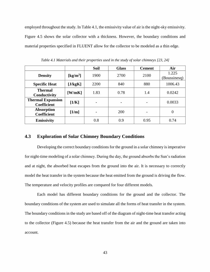
43

employed throughout the study. In Table 4.1, the emissivity value of air is the night-sky emissivity.

Figure 4.5 shows the solar collector with a thickness. However, the boundary conditions and

material properties specified in FLUENT allow for the collector to be modeled as a thin edge.

Table 4.1 Materials and their properties used in the study of solar chimneys [23, 24]

Soil Glass Cement Air

Density [kg/m3] 1900 2700 2100 1.225

(Boussinesq)

Specific Heat [J/kgK] 2200 840 880 1006.43

Thermal

Conductivity [W/mK] 1.83 0.78 1.4 0.0242

Thermal Expansion

Coefficient [1/K] - - - 0.0033

Absorption

Coefficient [1/m] - 200 - 0

Emissivity 0.8 0.9 0.95 0.74

4.3 Exploration of Solar Chimney Boundary Conditions

Developing the correct boundary conditions for the ground in a solar chimney is imperative

for night-time modeling of a solar chimney. During the day, the ground absorbs the Sun’s radiation

and at night, the absorbed heat escapes from the ground into the air. It is necessary to correctly

model the heat transfer in the system because the heat emitted from the ground is driving the flow.

The temperature and velocity profiles are compared for four different models.

Each model has different boundary conditions for the ground and the collector. The

boundary conditions of the system are used to simulate all the forms of heat transfer in the system.

The boundary conditions in the study are based off of the diagram of night-time heat transfer acting

to the collector (Figure 4.5) because the heat transfer from the air and the ground are taken into

account.

44

In all the models, ambient pressure and a temperature of 293 K is specified at the inlet and

outlet. These boundary conditions are chosen because the flow is driven by a pressure differential

in the system. Also, the chimney wall is modeled as adiabatic in all of the models, which is the

accepted boundary condition presented in the literature [12, 13, 14, 16, 18]. The DO radiation

model is incorporated into all of the simulations. The collector is considered as a semi-transparent

medium, but the ground and chimney are opaque boundaries. For each case, the simulations are

run transiently with a time step of 0.01 s and are run to 5 min. A transient method is necessary to

calculate the heat transfer over the system because it is dependent on time. The simulations are

compared at 5 min because the air flow through the chimney has developed. The velocity and

temperature profiles are representative of the shape and magnitude of the flow. As time progresses,

the temperature and velocity will vary but the shape and the magnitude of the profiles remain

consistent.

4.3.1 Description of Different Boundary Conditions

Four different combinations of collector and boundary conditions are used in this study.

The first case employs an adiabatic collector and the ground boundary is considered no-slip with

a constant heat flux of 800 W/m2. The chimney system is initialized to have a temperature of 293

K, a velocity of 0 m/s, and the pressure is initialized as ambient pressure

The second case also modeled the collector as adiabatic. However, the ground boundary is

modeled with mixed convective and radiative thermal properties and is considered no-slip. The

mixed boundary allows for the specification of internal and external emissivities and temperatures.

On the ground boundary, the internal and external values for the emissivity and the temperature

are the same because the values represent the radiation from the thermal storage. The temperature

45

and velocity are initialized to 293 K and 0 m/s, respectively. The initial pressure is considered to

be atmospheric.

The third case employs a mixed boundary condition for the collector and a constant ground

temperature of 300 K for the ground. The mixed boundary allows for radiative and convective

conditions to be specified on the collector as well as internal and external emissivities. For the

collector boundary, the external radiation represents the night sky radiation. The internal

emissivity and temperature correspond to the emissivity of the collector and the temperature inside

the solar chimney. The system is initialized to a temperature of 293 K and a velocity of 0 m/s. The

initial pressure is considered to be atmospheric.

The fourth, and final case, includes a layer of thermal storage. The thermal storage is made

up of a porous material with the same thermal properties as soil. The thermal storage is considered

to be a packed-bed with an average particle diameter of 2 mm and a porosity of 25%. Using the

equations included in Section 2.5, the viscous resistance in the bed is found to be 1.35 ×

109 1/𝑚2, and the inertial resistance is 8.4 × 104 1/𝑚. The bottom of the thermal storage has a

constant temperature of 300 K and the sides of the thermal storage are adiabatic. The collector

boundary is specified to have a mixed convective and radiative boundary condition. The

temperature in the entire system is initialized to 350 K to simulate the heat absorbed by the storage

during the day. The velocity is initialized to 0 m/s and the initial pressure is considered to be

atmospheric pressure. All of the specific boundary conditions are outlined in Table 4.2. The

emissivities of the materials can be found in Table 4.1.

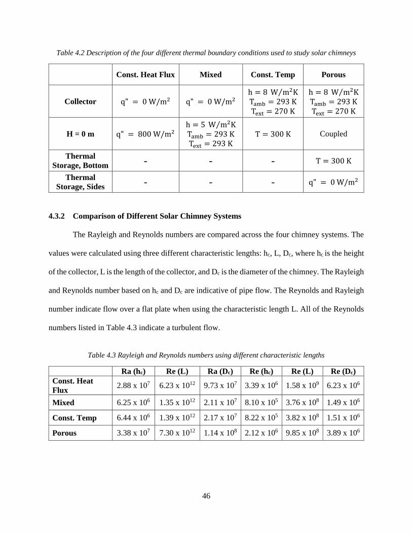
46

Table 4.2 Description of the four different thermal boundary conditions used to study solar chimneys

Const. Heat Flux Mixed Const. Temp Porous

Collector q" = 0 W/m2 q" = 0 W/m2

h = 8 W m2K⁄

Tamb = 293 K

Text = 270 K

h = 8 W m2K⁄

Tamb = 293 K

Text = 270 K

H = 0 m q" = 800 W/m2

h = 5 W m2K⁄

Tamb = 293 K

Text = 293 K

T = 300 K Coupled

Thermal

Storage, Bottom - - - T = 300 K

Thermal

Storage, Sides - - - q" = 0 W/m2

4.3.2 Comparison of Different Solar Chimney Systems

The Rayleigh and Reynolds numbers are compared across the four chimney systems. The

values were calculated using three different characteristic lengths: hc, L, Dc, where hc is the height

of the collector, L is the length of the collector, and Dc is the diameter of the chimney. The Rayleigh

and Reynolds number based on hc and Dc are indicative of pipe flow. The Reynolds and Rayleigh

number indicate flow over a flat plate when using the characteristic length L. All of the Reynolds

numbers listed in Table 4.3 indicate a turbulent flow.

Table 4.3 Rayleigh and Reynolds numbers using different characteristic lengths

Ra (hc) Re (L) Ra (Dc) Re (hc) Re (L) Re (Dc)

Const. Heat

Flux 2.88 x 107 6.23 x 1012 9.73 x 107 3.39 x 106 1.58 x 109 6.23 x 106

Mixed 6.25 x 106 1.35 x 1012 2.11 x 107 8.10 x 105 3.76 x 108 1.49 x 106

Const. Temp 6.44 x 106 1.39 x 1012 2.17 x 107 8.22 x 105 3.82 x 108 1.51 x 106

Porous 3.38 x 107 7.30 x 1012 1.14 x 108 2.12 x 106 9.85 x 108 3.89 x 106

47

Temperature and velocity profiles are also compared across the four chimney models to

analyze dissimilarities that arise using the different boundary conditions. Noticeable difference

arise when all of the data is evaluated next to each other. The most significant disparity in the

velocity between the models is the magnitude. The velocity contour in all the models are extremely

similar in shape, and a representative contour is shown in Figure 4.6. The most informative portion

of the velocity contours occurs in the center of the chimney structure, so Figure 4.6 only includes

a partial geometry.

Figure 4.6 Representative contour of the velocity magnitude [m/s] in a solar chimney

Figure 4.6 is the velocity contour for a chimney with a mixed ground boundary condition

and an adiabatic collector. A similar magnitude is observed when the collector is modeled as a

mixed boundary and thermal storage is taken into account. When a constant heat flux is applied to

the ground boundary, the velocity magnitude is much greater than what is shown in the Figure 4.6.

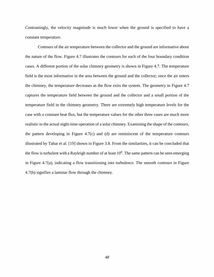
48

Contrastingly, the velocity magnitude is much lower when the ground is specified to have a

constant temperature.

Contours of the air temperature between the collector and the ground are informative about

the nature of the flow. Figure 4.7 illustrates the contours for each of the four boundary condition

cases. A different portion of the solar chimney geometry is shown in Figure 4.7. The temperature

field is the most informative in the area between the ground and the collector; once the air enters

the chimney, the temperature decreases as the flow exits the system. The geometry in Figure 4.7

captures the temperature field between the ground and the collector and a small portion of the

temperature field in the chimney geometry. There are extremely high temperature levels for the

case with a constant heat flux, but the temperature values for the other three cases are much more

realistic to the actual night-time operation of a solar chimney. Examining the shape of the contours,

the pattern developing in Figure 4.7(c) and (d) are reminiscent of the temperature contours

illustrated by Tahar et al. [19] shown in Figure 3.8. From the similarities, it can be concluded that

the flow is turbulent with a Rayleigh number of at least 108. The same pattern can be seen emerging

in Figure 4.7(a), indicating a flow transitioning into turbulence. The smooth contours in Figure

4.7(b) signifies a laminar flow through the chimney.

49

(a) Solar chimney with a constant heat flux

(b) Solar chimney with a mixed ground boundary

(c) Solar chimney with a constant ground temperature

(d) Solar chimney with thermal storage

Figure 4.7 Temperature contours of the airflow between the ground and the collector for solar chimneys

with different boundary conditions

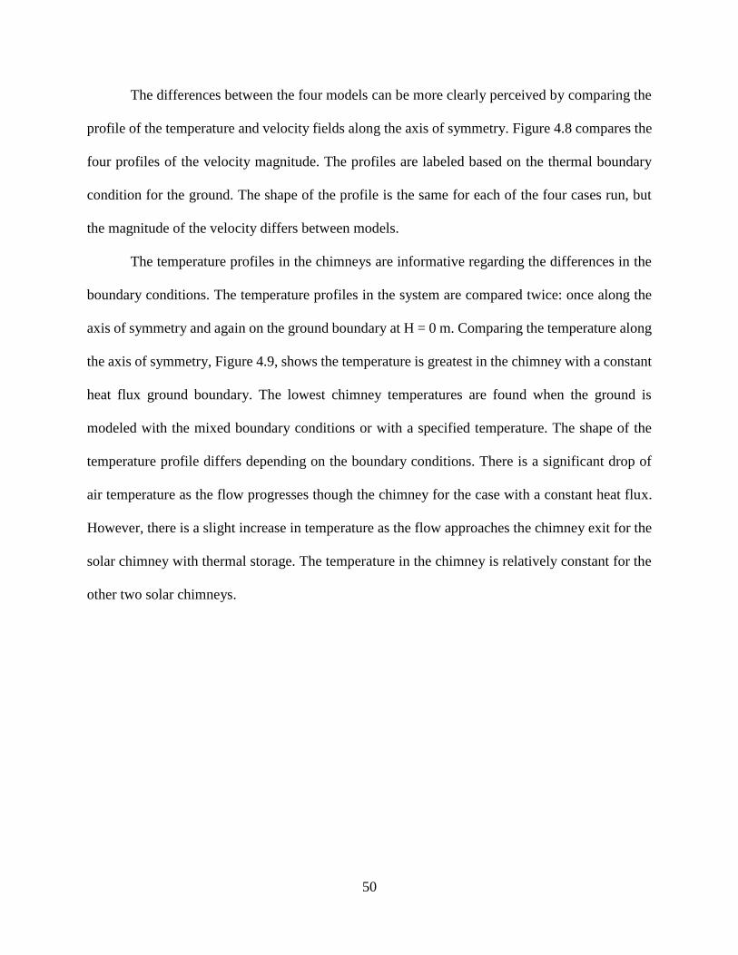
50

The differences between the four models can be more clearly perceived by comparing the

profile of the temperature and velocity fields along the axis of symmetry. Figure 4.8 compares the

four profiles of the velocity magnitude. The profiles are labeled based on the thermal boundary

condition for the ground. The shape of the profile is the same for each of the four cases run, but

the magnitude of the velocity differs between models.

The temperature profiles in the chimneys are informative regarding the differences in the

boundary conditions. The temperature profiles in the system are compared twice: once along the

axis of symmetry and again on the ground boundary at H = 0 m. Comparing the temperature along

the axis of symmetry, Figure 4.9, shows the temperature is greatest in the chimney with a constant

heat flux ground boundary. The lowest chimney temperatures are found when the ground is

modeled with the mixed boundary conditions or with a specified temperature. The shape of the

temperature profile differs depending on the boundary conditions. There is a significant drop of

air temperature as the flow progresses though the chimney for the case with a constant heat flux.

However, there is a slight increase in temperature as the flow approaches the chimney exit for the

solar chimney with thermal storage. The temperature in the chimney is relatively constant for the

other two solar chimneys.

51

Figure 4.8 Comparison of the instantaneous velocity magnitude at t = 5 min along the axis of symmetry

for the four different chimney boundary conditions

Figure 4.9 Instantaneous temperature comparison at t = 5 min along the axis of symmetry of the solar

chimney with different ground boundary conditions

52

The temperature along the edge H = 0 m is also influenced by the different boundary

conditions. Comparing the temperature profiles along H = 0 m, pictured in Figure 4.10, it is found

that the ground temperature is the greatest with a constant heat flux. The temperature of the ground

is the lowest when the ground was specified to have a convective heat transfer coefficient and

radiative properties. The temperature profile associated with the heat flux boundary condition is

extremely high and not congruent with the temperatures in an actual solar chimney.

Figure 4.10 Comparison of the instantaneous temperature at t = 3 min along the ground boundary for

four solar chimneys with different boundary conditions

Other properties compared include the flow rate through the system and the total heat

transfer rate. A summary of the results from the different simulations can be found in Table 4.4.

Comparing the flow rates, it is found that the greatest mass flow rate and volumetric flow rate

occur in the chimney system with the constant heat flux boundary. This finding is not surprising

because the heat flux boundary condition produced the greatest velocity in the chimney. The total

53

heat transfer in the system is also compared. FLUENT calculates the total heat transfer as the sum

of the convective and radiative heat flux. Table 4.4 presents the heat transfer rate across the ground

and collector boundaries and the total heat transfer rate in the system. The system’s total heat

transfer takes into account the fluxes entering and exiting the system, included the heat transfer at

the inlet and outlet. The heat transfer is negative if the heat is leaving the domain and if the heat is

added to the domain, the heat transfer is positive. For the heat transfer across the ground and the

collector, the domain is considered the boundary. However, for the total heat transfer, the domain

refers to the entire chimney system. The greatest amount of heat transfer occurs when the thermal

storage is applied. The heat transfer in the solar chimney with thermal storage includes the total

heat transfer in the porous material as well as the heat transfer in the chimney system.

Table 4.4 Summary of results comparing the four different boundary conditions

Const.

Heat Flux Mixed

Const.

Temp Porous

Max Temperature [K] 626.9 299.8 300 350

Max Velocity [m/s] 13.1 5.34 2.17 5.88

Volumetric Flow Rate [m3/s] 2.371 0.966 0.387 1.054

Mass Flow Rate [kg/s] 2.904 1.183 0.475 1.291

Heat Transfer Rate,

Ground [kW] 361.9 184.5 87.4 234.0

Heat Transfer Rate,

Collector [kW] 0 0 -87.1 -202.5

Total Heat Transfer in

Chimney System [kW] 35.7 184.5 0.040 -1,386.2

After studying the boundary conditions of the ground and collector and their influence on

the temperature and velocity fields in a solar chimney, conclusions can be made regarding the most

realistic boundary conditions. The best boundary for the solar collector is the mixed boundary

condition, allowing the user to specify a convective heat transfer coefficient and radiation

54

properties. The adiabatic boundary condition is un-realistic for the collector boundary because

there is multiple forms of heat transfer across the collector, as described in Figure 4.5.

The study helped to find the best boundary condition for the ground. Specifying the ground

as a constant heat flux is unrealistic because the amount of heat emitted by the ground will vary as

time progresses. Also, the amount of heat emitted by the ground will not be uniform across the

entire boundary. The mixed ground boundary is realistic because it accounts for convection and

radiation by the boundary. However, when the solar chimney was specified with mixed boundaries

for the ground and the collector, reverse flow occurred in the solar chimney. A constant

temperature boundary is unrealistic because the temperature of the ground will be influenced by

heat transfer from the ground and from the air moving across it. The best way to model the ground

boundary is to include a thermal storage layer modeled as a porous material.

It is necessary to include the thermal storage to model the ground because all three forms

of heat transfer are calculated between the ground and the air. The thermal storage also illustrates

how the heat releases from the ground over time. However, adding thermal storage to the solar

chimney system increases the computational intensity required by FLUENT to calculate the

solution.

4.4 Influence of the DO Radiation Model

Guo et al. [15] asserted that a radiation model is necessary to model a solar chimney in

order to correctly calculate the heat losses in the system. Two cases are simulated using FLUENT

to determine whether the radiation model is necessary in simulating the night-time operation of a

solar chimney. One case does not use a radiation model in the calculations, while the other

incorporates the DO radiation model. Although FLUENT has five different radiation models, only

55

the DO model allows for materials to be considered semi-transparent. Transparency is an important

material feature that needs to be captured in modeling the solar collector.

In the radiation study, the ground is modeled with a constant temperature and the collector

is modeled with a convective heat transfer coefficient and radiative properties. Thermal storage is

not included in the ground model because the purpose of the radiation study focuses on how air

properties are impacted by the radiation model. To decrease computational costs, the heat transfer

from the ground is approximated using the constant temperature boundary condition described

under “Const. Temp” in Table 4.2. The radiation systems are initialized to a temperature field of

293 K, a velocity field of 0 m/s, and ambient pressure.

The solar chimneys are simulated using a transient time stepping method and calculated

through five minutes. At this point in time, significant differences have developed between the two

models. Profiles of the temperature and the velocity through the system are compared to analyze

the variations associated with incorporating the DO radiation model. Comparing the velocity

magnitude, Figure 4.11, the velocity predicted with the radiation model is approximately three

times greater than the velocity magnitude in the system without it. There is also a variance in the

profile shape, which could be influenced by the existence of reversed flow at the inlet in the

chimney without a radiation model.

Temperature profiles also portray differences in the two models. Figure 4.12 compares the

temperature along the axis of symmetry in the two models. The temperature is greater in the model

incorporating the radiation model. Because there is no solar irradiation during the night, heat from

the system escapes through the collector. The amount of energy absorbed by the collector and the

emissivity of the collector material are only taken into account when the DO radiation model is

56

applied. The increase of heat loss in the system by not including a radiation model is illustrated in

a lower temperature in the chimney.

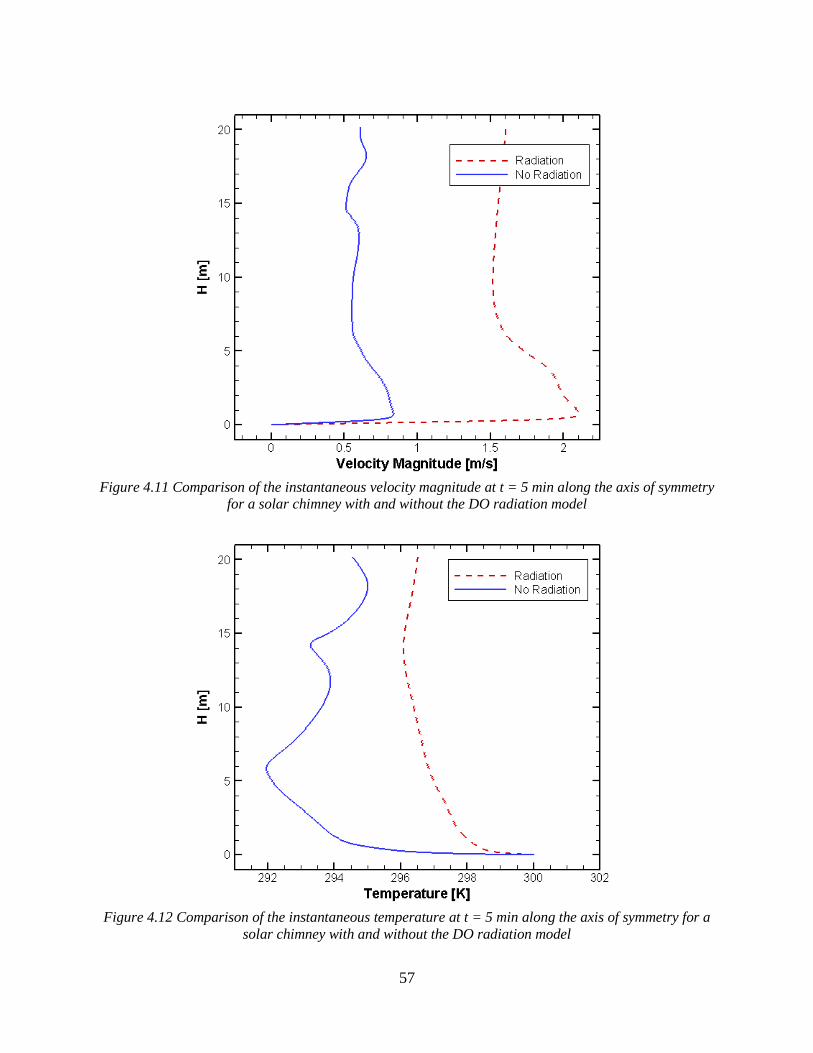
57

Figure 4.11 Comparison of the instantaneous velocity magnitude at t = 5 min along the axis of symmetry

for a solar chimney with and without the DO radiation model

Figure 4.12 Comparison of the instantaneous temperature at t = 5 min along the axis of symmetry for a

solar chimney with and without the DO radiation model

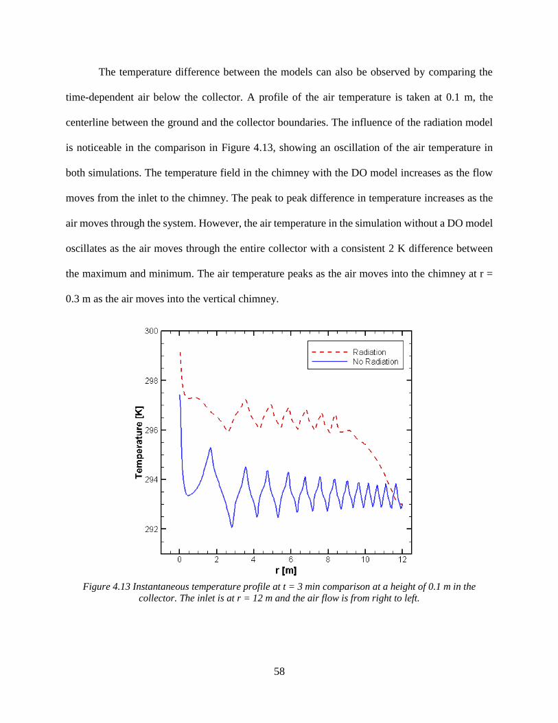
58

The temperature difference between the models can also be observed by comparing the

time-dependent air below the collector. A profile of the air temperature is taken at 0.1 m, the

centerline between the ground and the collector boundaries. The influence of the radiation model

is noticeable in the comparison in Figure 4.13, showing an oscillation of the air temperature in

both simulations. The temperature field in the chimney with the DO model increases as the flow

moves from the inlet to the chimney. The peak to peak difference in temperature increases as the

air moves through the system. However, the air temperature in the simulation without a DO model

oscillates as the air moves through the entire collector with a consistent 2 K difference between

the maximum and minimum. The air temperature peaks as the air moves into the chimney at r =

0.3 m as the air moves into the vertical chimney.

Figure 4.13 Instantaneous temperature profile at t = 3 min comparison at a height of 0.1 m in the

collector. The inlet is at r = 12 m and the air flow is from right to left.

59

The temperature and velocity are greater in the system with the radiation model, which

contrasts with the findings by Guo et al. [15] that modeled a solar chimney during the day where

radiation from the Sun is a significant source of heat. During the day, correctly calculating the heat

transfer on the collector has a greater impact on the system because the flow is driven by the Sun’s

energy passing through the collector. Without a radiation model, the heat losses in the collector

and the amount of energy absorbed by the collector are incorrectly analyzed. The differences in

the heat transfer in the system are described in Table 4.5. There is significantly more heat transfer

across the boundaries when radiation is appropriately accounted for. The inappropriate

calculations lead to an increase in the system’s temperature and a difference in the heat transfer in

the entire system.

Table 4.5 Comparison of solar chimney systems with and without the DO radiation model

With DO Model Without DO Model

Maximum Velocity [m/s] 2.144 0.837

Volumetric Flow Rate [m3/s] 0.387 0.144

Mass Flow Rate [kg/s] 0.475 0.176

Heat Transfer Rate, Ground [kW] 87.4 5.276

Heat Transfer Rate,

Collector [kW] -87.1 -5.243

Total Heat Transfer in

Chimney System [kW] 0.040 0.184

A radiation model impacts the temperature profile of the system because the heat loss in

the system is incorrectly calculated when the radiation model is neglected. During the night,

calculating the heat loss incorrectly leads to a lower system temperature; however, higher

temperatures are found when solar radiation is added to the system. Table 4.5 illustrates the

differences that occur when the radiation model is included in FLUENT. The conclusion that the

60

radiation model greatly impacts the temperature and velocity profiles in the system is congruent.

It is concluded that the DO radiation model is necessary to accurately simulate airflow through a

solar chimney.

4.5 Dispersion of Heat over Time

In the study conducted to determine the best ground boundary conditions for a solar

chimney, a conclusion was reached indicating that thermal storage is needed to best model the

night-time operation of a solar chimney. The thermal storage stores heat during the day and

releases it during the night. FLUENT was used to model a chimney system with thermal storage

to observe how long it would take for the heat stored by the ground to dissipate.

In the study, the geometry shown in Figure 4.2 is used. The collector is considered a semi-

transparent material with the radiative and convective boundary conditions. The thermal storage

is modeled as a porous medium to account for heat transfer by radiation, convection, and

conduction. The exact boundary conditions used in the study are described in Table 4.2 under

“Porous”. The packed-bed material used to model the thermal storage is described in Section 4.3.1.

The bottom of the thermal storage is considered a boundary with a constant temperature of 300 K

and the sides of the thermal storage are specified as adiabatic. The inlet and outlet of the chimney

are considered to be at atmospheric pressure with a temperature of 293 K, and the chimney wall is

considered adiabatic. During night-time operation of a solar chimney power-plant, the heat stored

in the ground is emitted into the air. To account for the ground absorbing the heat during the day,

the temperature field is initialized to 350 K. The velocity in the system is initialized to 0 m/s and

the initial pressure is atmospheric.

A transient simulation is able to calculate the dispersion of heat through the system over

time. The change in temperature and velocity in the chimney can be observed as time progresses.

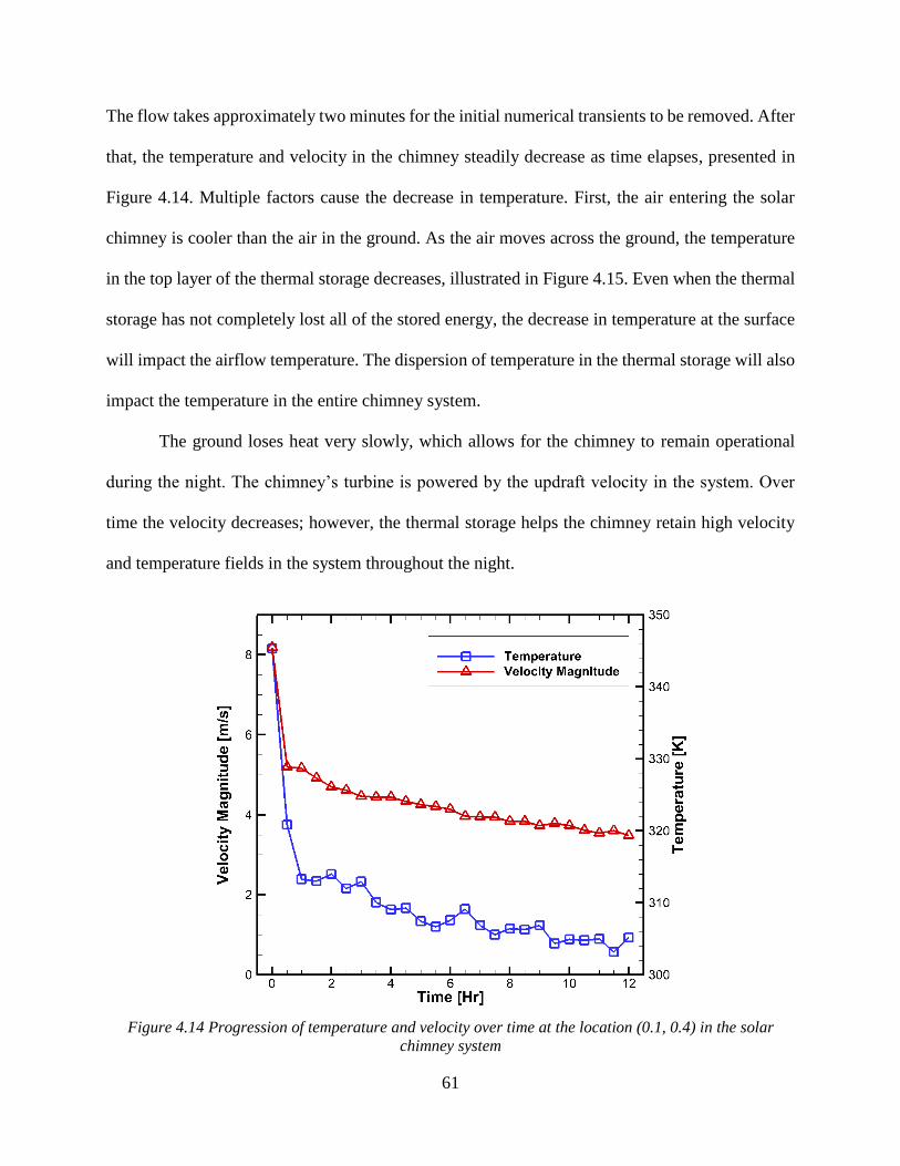
61

The flow takes approximately two minutes for the initial numerical transients to be removed. After

that, the temperature and velocity in the chimney steadily decrease as time elapses, presented in

Figure 4.14. Multiple factors cause the decrease in temperature. First, the air entering the solar

chimney is cooler than the air in the ground. As the air moves across the ground, the temperature

in the top layer of the thermal storage decreases, illustrated in Figure 4.15. Even when the thermal

storage has not completely lost all of the stored energy, the decrease in temperature at the surface

will impact the airflow temperature. The dispersion of temperature in the thermal storage will also

impact the temperature in the entire chimney system.

The ground loses heat very slowly, which allows for the chimney to remain operational

during the night. The chimney’s turbine is powered by the updraft velocity in the system. Over

time the velocity decreases; however, the thermal storage helps the chimney retain high velocity

and temperature fields in the system throughout the night.

Figure 4.14 Progression of temperature and velocity over time at the location (0.1, 0.4) in the solar

chimney system

62

The solution was calculated transiently for a total of twelve hours, simulating the time

during the night where there would be little or no solar irradiation. During the elapsed time, the

amount of heat stored in the thermal storage did not completely dissipate, shown in Figure 4.15.

Unfortunately, the results gathered in the simulation are not realistic. Over the twelve hours, the

temperature in the thermal storage should have completely cooled so a gradient is visible in the

thermal storage. Because the majority of the thermal storage still has an extremely high

temperature, it can be ascertained that the porous ground is not modeled correctly.

Despite the incorrect modeling the thermal storage, conclusions regarding the inclusion of

thermal storage can be made. Thermal storage retains energy during and releases it back into the

air stream throughout the night. The additional heat increases the airflow through the chimney

system, meaning the plant can harvest energy from the updraft velocity during the night. It is

necessary to include the porous material as the ground because FLUENT can calculate the

convective, conductive, and radiative heat transfer between the ground and the air.

63

2 Hour

4 Hour

6 Hour

8 Hour

10 hour

12 Hour

Figure 4.15 Contours illustrating the progression of temperature [K] in a solar chimney with thermal storage over time

64

Chapter 5: Optimizing the Solar Chimney System

The following chapter will discuss different ways to increase the airflow through a solar

chimney. Alternate geometric configurations using clusters of shorter chimneys will be presented.

The results from the study will be compared to a single chimney geometry. Then, the use of passive

advection wells dug into the thermal storage will be explored.

5.1 Chimney Clusters

A cluster geometry refers to the use of multiple chimneys with the same combined height

as a single chimney. The purpose of using multiple chimneys is to reduce the loftiness of a solar

chimney without decreasing the amount of airflow through the system. Two different chimney

clusters are used in the study.

5.1.1 Chimney Geometry and Boundary Conditions

The first cluster has a total of five chimneys, each with a height of 4 m. The cross-sectional

area of each chimney’s outlet is 0.25 m2 for a total outlet area of 1.25 m2. Figure 5.1 shows the

five-chimney geometry and the top view of the chimney outlet. The four-chimney system can also

be represented by the geometry pictured in Figure 5.1. In a four-chimney structure, four towers are

constructed about a central support which replaces the central (and fifth) chimney. Each chimney

has a height of 5 m, for a total combined height of 20 m. The outlet area of each chimney is 0.0676

m2 for a total outlet area of 0.27 m2. The inlet area of the solar system chimney is calculated by

multiplying the outer perimeter of the solar collector by its height. Both the four-chimney and five-

chimney clusters have inlet areas of 17 m2.

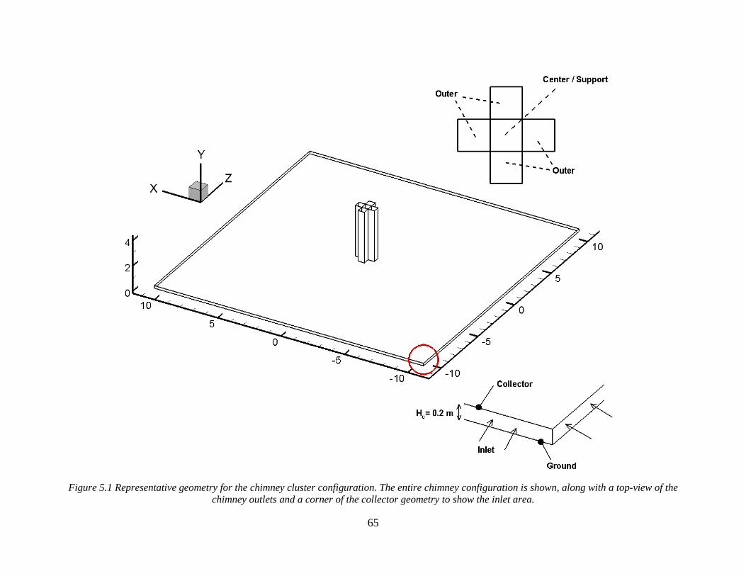
65

Figure 5.1 Representative geometry for the chimney cluster configuration. The entire chimney configuration is shown, along with a top-view of the

chimney outlets and a corner of the collector geometry to show the inlet area.

66

The same boundary conditions are used across all the chimney configurations in order to

compare the temperature and velocity fields in the different geometries. The inlets and outlets are

specified to be at atmospheric pressure with an ambient temperature of 293 K. All of the chimney

walls are considered adiabatic. The collector boundary is considered no-slip and modeled using

the mixed convective and radiative boundary condition described in Table 4.2. The ground is a no-

slip boundary with a constant temperature of 300 K. Ground with thermal storage is not

incorporated in this part of the study as a way to reduce the computational costs because of the

large three-dimensional system used to model the chimney clusters. The temperature field in the

system is initialized at 293 K, the velocity field is initialized to 0 m/s, and the initial pressure is

atmospheric.

5.1.2 Airflow through Chimney Clusters

The entire cluster geometry is modeled three-dimensionally study the flow through the

chimneys. Because of the large computational effort required by FLUENT, only three minutes of

flow time is calculated. The instantaneous streamlines are analyzed at three minutes to determine

flow patterns through each systems.

The first chimney system investigated is the cluster of five chimneys. The ambient air

moves from the inlet into the five chimneys. Surveying the streamlines in Figure 5.2, it can be seen

that the flow is fairly symmetrical. Figure 5.2 also includes a two-dimensional slice capturing the

streamlines of the three chimneys located along Z = 0 m. The snapshot of the streamlines shows

how the air is moving through the three chimneys. The warmer air (air closer to the collector) is

flowing into the outer chimneys, and the cooler air is moving into the center chimney. The velocity

of the air is greatest in the center chimney because it is getting the largest amount of airflow.

67

Figure 5.2 Streamlines depicting the instantaneous path of the air moving through the five chimney

geometry after one minute. Flow through the three chimneys along the slice Z = 0 m is also captured.

The symmetry in the system is verified by comparing the velocity and temperature profiles

located at the centerlines of the five chimneys. Figure 5.3 and Figure 5.4 show the centerline

profiles of the velocity magnitude and temperature, respectively. The center chimney is located on

the X – Z axis at (0, 0). The four outer chimneys are labeled by their location relative to the center

chimney on the X – Z axis. The profiles associated with the four outer chimneys are coincidental

for both the temperature and velocity fields. The conclusion suggests that future studies can model

a quarter of the five-chimney geometry using symmetry boundary conditions to reduce the

computational costs of the system.

68

Figure 5.3 Profile of the velocity magnitude along the centerline of each chimney in the five-chimney

cluster

Figure 5.4 Temperature profile at the centerline of each chimney in the five-chimney cluster

69

Streamlines through the four-chimney geometry are also studied. Captured in Figure 5.5,

the streamlines once again indicate a symmetric flow field through the solar chimney system.

Observing the streamlines captured along the slice Z = 0 m, it is observed that there is no airflow

passing underneath the support. The phenomenon means the air is flowing up the chimney closest

to inlet that the air used to enter the system.

Figure 5.5 Instantaneous streamlines in a four-chimney solar chimney after one minute. Streamlines

along the slice Z = 0 m are also shown

The temperature and velocity profiles of each chimney are compared along the centerline.

The profiles are extremely similar to the profiles of the four outer chimneys shown in Figure 5.3

and Figure 5.4 The finding indicates that future studies can use a quarter of the geometry with

symmetry boundary conditions is needed to model the four-chimney cluster.

70

5.1.3 Comparison of Chimney Designs

The instantaneous airflow through the two cluster geometries are compared with the

airflow through a single, axisymmetric chimney with no thermal storage after three minutes. The

axisymmetric, single-tower geometry is shown in Figure 4.2. Two axisymmetric chimneys are

used in the comparison study, the original chimney with an inlet area of 15 m2 and a second

chimney with an inlet area of 17 m2. The second axisymmetric geometry was created because the

cluster geometries all have an inlet area of 17 m2. The geometric differences are described in Table

5.1. The temperature and velocity profiles are compared along centerlines of the different chimney

geometries. Two profiles are used to represent the airflow through different chimneys in the five-

chimney geometry: the centerline of the center chimney and a centerline of one of the four outer

chimneys. Only one centerline is used to represent the four-chimney geometry.

Table 5.1 Geometric differences in the four different chimney designs studied

Axisym (15) Axisym (17) 5 Chimney

Cluster

4 Chimney

Cluster

Chimney Height [m] 20 20 4 5

Inlet Area [m2] 15.08 16.96 17.00 17.00

Single Chimney

Outlet Area [m2] 0.283 0.283 0.250 0.0676

Total Outlet Area [m2] 0.283 0.283 1.250 0.270

There is a significant difference in the centerline velocity across the four chimneys. The

greatest velocity occurs in the original chimney, Axisym (15), in Figure 5.6. The large velocities

can be attributed to the smaller inlet area and to the geometric configuration of only having one

chimney. The other axisymmetric chimney, Axisym (17), has an extremely similar velocity profile

to the original axisymmetric geometry. There are also differences in the velocity centerlines in the

five-chimney geometry. The central chimney has a much greater velocity than one of the outer

71

chimneys in the same geometry. The centerline velocity through the geometry with only four

chimneys is very similar to the velocity profile of the center chimney in the five-chimney

configuration. However, the magnitude of the velocity in the four-chimney velocity is slightly

lower.

The temperature profiles in Figure 5.7 reveal additional information regarding the flow in

the chimneys. The chimneys with the highest temperature is the four-chimney cluster. The

temperature in the four-chimney system is fairly constant as the flow progresses through the

chimney. The temperature in the center chimney of the five-chimney system is greater than the

temperature in the outer chimneys in the same geometry, which is to be expected. The flow

temperatures in the center chimney in the five-chimney configuration and in the four-chimney are

greater than the temperature in the original axisymmetric geometry.

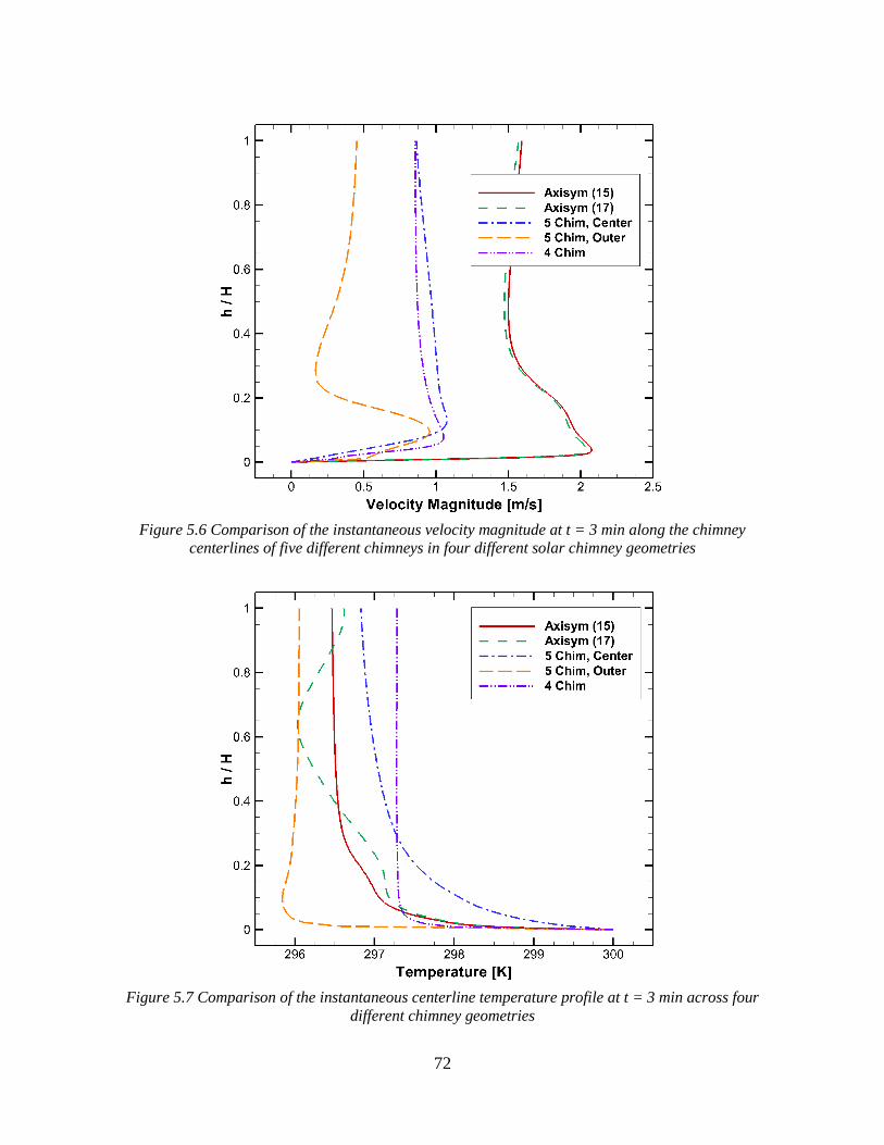
72

Figure 5.6 Comparison of the instantaneous velocity magnitude at t = 3 min along the chimney

centerlines of five different chimneys in four different solar chimney geometries

Figure 5.7 Comparison of the instantaneous centerline temperature profile at t = 3 min across four

different chimney geometries

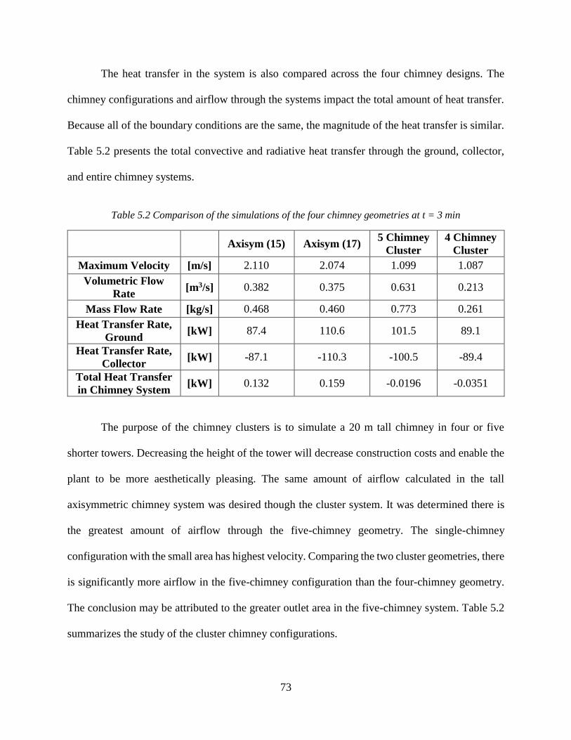
73

The heat transfer in the system is also compared across the four chimney designs. The

chimney configurations and airflow through the systems impact the total amount of heat transfer.

Because all of the boundary conditions are the same, the magnitude of the heat transfer is similar.

Table 5.2 presents the total convective and radiative heat transfer through the ground, collector,

and entire chimney systems.

Table 5.2 Comparison of the simulations of the four chimney geometries at t = 3 min

Axisym (15) Axisym (17) 5 Chimney

Cluster

4 Chimney

Cluster

Maximum Velocity [m/s] 2.110 2.074 1.099 1.087

Volumetric Flow

Rate [m3/s] 0.382 0.375 0.631 0.213

Mass Flow Rate [kg/s] 0.468 0.460 0.773 0.261

Heat Transfer Rate,

Ground [kW] 87.4 110.6 101.5 89.1

Heat Transfer Rate,

Collector [kW] -87.1 -110.3 -100.5 -89.4

Total Heat Transfer

in Chimney System [kW] 0.132 0.159 -0.0196 -0.0351

The purpose of the chimney clusters is to simulate a 20 m tall chimney in four or five

shorter towers. Decreasing the height of the tower will decrease construction costs and enable the

plant to be more aesthetically pleasing. The same amount of airflow calculated in the tall

axisymmetric chimney system was desired though the cluster system. It was determined there is

the greatest amount of airflow through the five-chimney geometry. The single-chimney

configuration with the small area has highest velocity. Comparing the two cluster geometries, there

is significantly more airflow in the five-chimney configuration than the four-chimney geometry.

The conclusion may be attributed to the greater outlet area in the five-chimney system. Table 5.2

summarizes the study of the cluster chimney configurations.

74

5.2 Passive Advection Wells

Another way to amplify the airflow through a solar chimney is to accelerate the airflow by

increasing the air temperature. The temperature can be increased by extracting the absorbed heat

from the thermal storage through the use of wells. It is theorized that the wells will draw the hot

air from the ground into the well and disperse the heat into the airstream.

5.2.1 Well Geometry and Boundary Conditions

A solar chimney system with a single chimney and thermal storage is used to test the

advection wells. A three-dimensional geometry modeling a quarter of the solar chimney is used in

the simulation. The study discussed in Chapter 4 justifies the use of symmetry boundary conditions

in a solar chimney because it proved that the flow was symmetric. In the full three-dimensional

model, there are nine wells evenly spaced under the collector. Each well has a depth of 0.5 m. The

wells have a square opening at the top and bottom with side lengths of 0.1 m. Only one complete

well is modeled because of the symmetry boundary conditions, but half of two different wells and

a quarter of another well are also included in the geometry. The half wells are located along X = 0

m and Z = 0 m, where the symmetry boundary is located. The quarter well is located directly under

the chimney structure and has two sides specified as symmetric. Figure 5.8 shows the entire

quarter-chimney geometry and the full well geometry.

75

Figure 5.8 Geometry used to model the flow through a solar chimney with passive advection wells.

Included is a geometric representation of a well.

The boundary conditions to model the chimney system are the optimal conditions

determined in Section 4.3. The air enters the system through an inlet specified at ambient pressure

with a temperature of 293 K. The air exits the system via an outlet set at ambient pressure and a

temperature of 293 K. The chimney walls are considered adiabatic, and the solar collector is

modeled as a no-slip boundary with additional radiative and convective boundary conditions,

which are described in Table 4.2. Thermal storage is incorporated into the simulation. The porous

76

material properties used to model the ground is described in Section 4.3.1. The top of the thermal

storage is a no-slip surface and the boundary is considered thermally coupled between the ground

and the air. The bottom of the storage layer has a specified temperature of 300 K and is considered

no-slip. The sides of the thermal storage are adiabatic. The sides of the advection wells are modeled

as adiabatic and are made out of aluminum. The material choice is based on an idea to construct

the wells out of recycled aluminum cans. The top and the bottom of the wells are thermally coupled

boundary conditions. The sides of the entire geometry along X = Z = 0 m are modeled as symmetry

boundaries. The entire domain is initialized with a zero-velocity field and at atmospheric pressure.

The temperature is initialized at 350 K as a way to capture the energy absorbed by the thermal

storage throughout the day.

5.2.2 Airflow in a Solar Chimney with Wells

The well configuration has been simulated transiently for three minutes to study the initial

airflow through the system. The study of the thermal storage system in the previous chapter

determined that the initial numerical transients in the flow are no longer present after two minutes

of calculations. Only three minutes of time are calculated because it is believed that the airflow in

the wells will not change drastically when the simulation is run longer.

The purpose of the wells is to draw the heat from the ground up through the wells and into

the airstream passing through the chimney system. Unfortunately, the wells do not work as

theorized. Analyzing the flow in the system, the air is being drawn into the wells and pushed out

into the ground. Air also forms eddies inside and next to the wells. Instantaneous streamlines at 3

minutes in Figure 5.9 depict the air circulating in the thermal storage next to the wells. The

magnification of the center well in Figure 5.9 shows the air circulating in the well with a low

velocity. The air that does pass through the wells exits the bottom of the well into the thermal

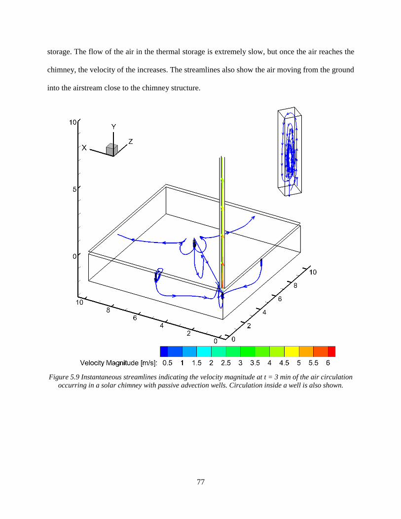
77

storage. The flow of the air in the thermal storage is extremely slow, but once the air reaches the

chimney, the velocity of the increases. The streamlines also show the air moving from the ground

into the airstream close to the chimney structure.

Figure 5.9 Instantaneous streamlines indicating the velocity magnitude at t = 3 min of the air circulation

occurring in a solar chimney with passive advection wells. Circulation inside a well is also shown.

78

The temperature of the air is impacted by the material it is flowing through, shown in Figure

5.10. When the air is flowing through the porous ground, the air has a very high temperature

because of the high temperature in the ground. The air moving in the wells, under the collector and

through the chimney have a lower temperature because the air entering the system is at a lower

temperature.

Figure 5.10 Instantaneous streamlines showing the temperature of the air at t = 3 min occurring in a

solar chimney with wells. Circulation inside a well is also shown.

79

The airflow under the collector is also analyzed. Streamlines in Figure 5.11 show the

velocity of the air moving from the inlet to the chimney. The air is moving extremely slowly until

the flow enters the chimney structure.

Figure 5.11 Velocity magnitude of the airflow through the collector in a solar chimney with passive

advection wells.

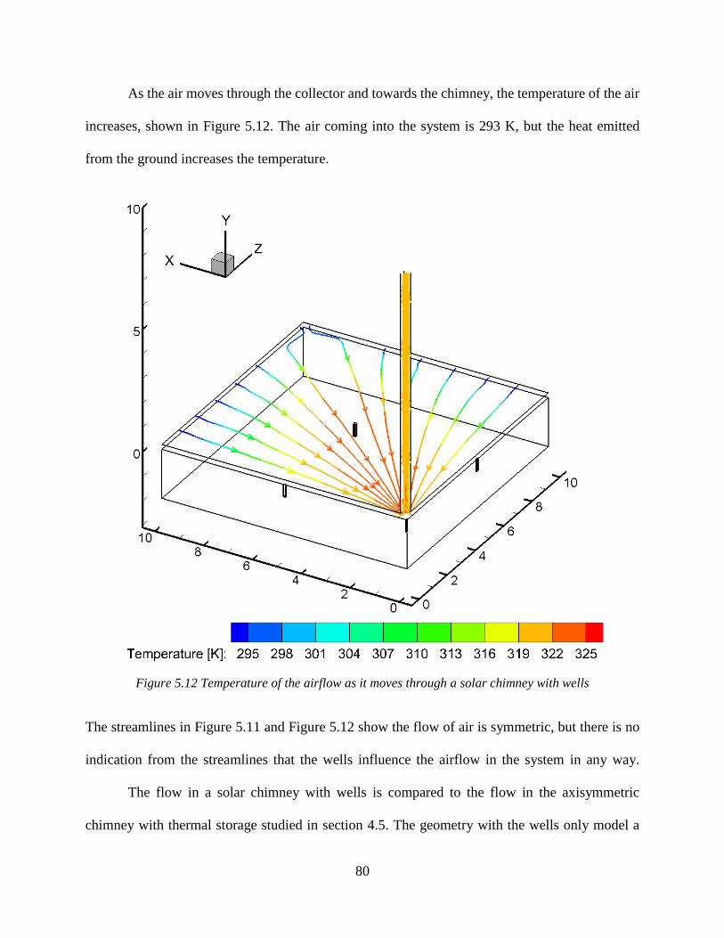
80

As the air moves through the collector and towards the chimney, the temperature of the air

increases, shown in Figure 5.12. The air coming into the system is 293 K, but the heat emitted

from the ground increases the temperature.

Figure 5.12 Temperature of the airflow as it moves through a solar chimney with wells

The streamlines in Figure 5.11 and Figure 5.12 show the flow of air is symmetric, but there is no

indication from the streamlines that the wells influence the airflow in the system in any way.

The flow in a solar chimney with wells is compared to the flow in the axisymmetric

chimney with thermal storage studied in section 4.5. The geometry with the wells only model a

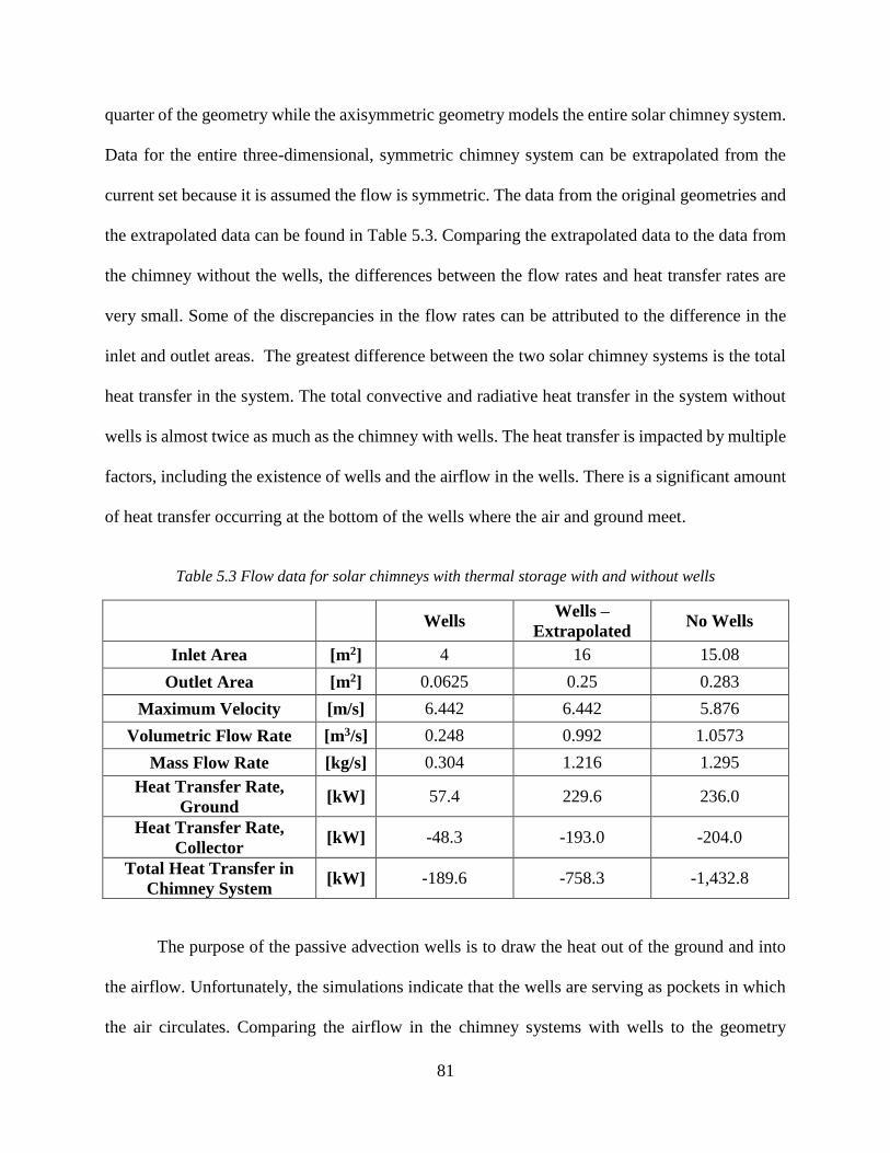
81

quarter of the geometry while the axisymmetric geometry models the entire solar chimney system.

Data for the entire three-dimensional, symmetric chimney system can be extrapolated from the

current set because it is assumed the flow is symmetric. The data from the original geometries and

the extrapolated data can be found in Table 5.3. Comparing the extrapolated data to the data from

the chimney without the wells, the differences between the flow rates and heat transfer rates are

very small. Some of the discrepancies in the flow rates can be attributed to the difference in the

inlet and outlet areas. The greatest difference between the two solar chimney systems is the total

heat transfer in the system. The total convective and radiative heat transfer in the system without

wells is almost twice as much as the chimney with wells. The heat transfer is impacted by multiple

factors, including the existence of wells and the airflow in the wells. There is a significant amount

of heat transfer occurring at the bottom of the wells where the air and ground meet.

Table 5.3 Flow data for solar chimneys with thermal storage with and without wells

Wells Wells –

Extrapolated No Wells

Inlet Area [m2] 4 16 15.08

Outlet Area [m2] 0.0625 0.25 0.283

Maximum Velocity [m/s] 6.442 6.442 5.876

Volumetric Flow Rate [m3/s] 0.248 0.992 1.0573

Mass Flow Rate [kg/s] 0.304 1.216 1.295

Heat Transfer Rate,

Ground [kW] 57.4 229.6 236.0

Heat Transfer Rate,

Collector [kW] -48.3 -193.0 -204.0

Total Heat Transfer in

Chimney System [kW] -189.6 -758.3 -1,432.8

The purpose of the passive advection wells is to draw the heat out of the ground and into

the airflow. Unfortunately, the simulations indicate that the wells are serving as pockets in which

the air circulates. Comparing the airflow in the chimney systems with wells to the geometry

82

without wells, there is very little difference in the airflow. However, the incorrect modeling of the

porous material may attribute to the airflow in the wells. Also, running the simulation longer is

necessary to give a conclusive decision about the effectiveness of the wells.

83

Chapter 6: Conclusions and Recommendations

6.1 Conclusion

The focus of the study was to develop boundary conditions to simulate the night-time

operation of a solar chimney and optimize the chimney design by comparing alternate chimney

configurations. Simulations were performed using the commercial CFD software FLUENT, which

solved the Navier-Stokes equations using the Boussinesq approximation. The realizable 𝑘 − 𝜀

turbulence model and the DO radiation model were employed in FLUENT. The packed-bed porous

model was used to simulate the thermal storage layer of the ground. ICEM was used to create the

computational domains, which were solved using the SIMPLE discretization.

A two-dimensional axisymmetric solar chimney was used in an investigation to determine

appropriate night-time boundary conditions. The inlet and outlet were specified at atmospheric

pressure with an ambient temperature of 293 K and the chimney wall was considered adiabatic in

all of the different configurations. Four cases with different boundary conditions for the collector

and the ground were simulated and compared. It was concluded that a no-slip, mixed convective

and radiative boundary was the best way to model the solar collector. The ground was best modeled

using a thermal storage layer of a porous material. The porosity allows for the calculation of

convective, radiative, and conductive heat transfer between the ground and the air. The bottom of

the thermal storage layer had a constant temperature of 300 K and the sides were considered

adiabatic. After running the model with thermal storage for twelve hours, the heat had not fully

diffused from the thermal storage. The conclusion was made that more work is needed to develop

an appropriate model for the porous material.

The necessity of the DO radiation model was also studied by comparing two axisymmetric

systems. The DO radiation model was chosen because it is the only radiation model that accounts

84

for the transparency of materials, and transparency is an important feature of the solar collector.

Comparing the temperature and velocity fields in the systems allowed for the study of how the

radiation model impacts the system. During a night-time simulation, the temperature in the system

was greatest when the radiation model was employed. Without the radiation model, the energy

losses on the collector (and other surfaces) are calculated incorrectly and allows extra heat to

escape the system. It was concluded that is essential to use the DO radiation model to properly

calculate the heat transfer in the solar chimney system.

Different geometric configurations of chimneys were compared as part of the study to

increase the amount of airflow through a chimney. Clusters of four and five chimneys with a total

combined height of 20 m were studied. All of the chimney walls were specified as adiabatic, and

the collector was considered to have radiative and convective boundary conditions. To save

computational costs, the ground was modeled with a constant 300 K temperature. Comparing the

chimney clusters with the single, axisymmetric chimney after three minutes of flow time, it was

found that the mass flow rate in the system increases when the five-chimney cluster is employed.

The maximum velocity was also compared, and it was found that the greatest velocity occurred in

the original axisymmetric chimney. The maximum velocity occurs in the bottom of chimney

structure where the air moves from under the collector into the chimney. It is important to have a

high velocity near at the collector-chimney junction because that is the location of a turbine when

it is added to the system. The turbine be powered by the updraft velocity, which means the greater

the velocity, the faster the turbine can turn to generate power. The solar tower in Manazares, Spain

had a maximum output of 50 kW of power [3]. The theoretical power, 𝑃, of the system can be

𝑃 =

1

2𝜋𝜉𝜌𝑟2𝑣3 ( 45 )

85

where 𝜉 is the efficiency of the turbine, and 𝑟 is the radius of the chimney [25]. Assuming an

average efficiency of 40% and a single chimney geometry, a velocity of 89.7 m/s is required to get

a power output of 50 kW. The velocities presented in this thesis are much lower than the required

velocity. Calculating the power output using the maximum velocity in the single, axisymmetric

chimney, the power is 0.64 W. This is an extremely small power output. However, more research

into simulating the best chimney system and accurately calculating the heat transfer will increase

the updraft velocity and the power output.

The use of passive advection wells were studied as a way to extract more heat from the

thermal storage in the ground. Theoretically, the wells would force air out of the ground and into

the passing air stream with a higher temperature. Unfortunately, simulating a single-chimney

geometry with wells showed air creating eddies in the wells. The eddies might be caused by

incorrect modeling of the porous thermal storage or by not running the simulation long enough.

A solar chimney is a difficult system to simulate. The study done determined the best

boundary conditions to use while modeling a solar chimney in FLUENT. Different ways to

increase fluid flow through a solar chimney were also studied. Many areas of this study can be

improved to design an efficient solar chimney that is operational twenty-four hours a day and is

more visually appealing (e.g., has a shorter height).

6.2 Recommendations for Future Work

There are still many areas to explore in the area of CFD modeling of a solar chimney. One

of the main focuses of the study was to determine realistic boundary conditions to model the solar

chimney. The study included simulating thermal storage using the packed-bed model of a porous

material. Unfortunately, an incorrect assumption was made in the study which prevented heat from

dissipating from the thermal storage after twelve hours. The work can be continued to develop a

86

more accurate model of the thermal storage. The study can also be expanded by studying the effect

different materials have on the thermal storage to determine the best material that stores the most

heat.

Once a better model for the thermal storage is developed, many areas of this study can be

improved. Simulations involving the passive-advection wells can be reconsidered to determine

better modeling techniques of the thermal storage and the air moving through the wells. The wells

can also be increased in diameter or height to determine how the size of wells impact air flow. The

use of forced-advection in a solar chimney system can also be studied. Forced advection wells

inject air into the ground to increase the amount of air moving from the ground into the air. A

system comprised of both passive and forced wells can be analyzed to determine how the

combination of wells impacts the airflow through the solar chimney system.

Additional geometric configurations of solar chimneys can be studied to expand on the

study of optimizing the design of the solar chimney. The goal of the study was to decrease the

height of the chimney to save on material costs and to improve on the appearance. A new wrapped

geometry can be considered. The wrapped geometry would simulate a twenty meter tower with

only five meters of physical height by adding curves to the chimney tower. The chimney curve

would allow for the chimney to expand in the radial direction, as well as vertically. The final

chimney and collector structure would be in the approximate shape of an S instead of an L, and the

total tower height will be reduced. The theory behind the wrapped tower can be tested by

comparing the velocity and temperature fields of the wrapped geometry to that of the axisymmetric

geometry. The wrapped tower can also be exploited in the cluster geometry creating clusters of

wrapped chimneys instead of straight chimneys. Clusters of wrapped towers may greatly improve

87

airflow through a solar chimney because there would be four towers each simulating a 20 m

chimney instead of a cluster of shorter chimneys with a total combined height of 20 m.

Finally, the addition of a turbine to the solar chimney system can be studied. The addition

of the turbine will allow the entire system to be considered a power plant and the efficiency can

be studied. Once the optimal chimney design and a turbine is selected for the system, the system

can be run in FLUENT for twenty-four hours using the solar-ray tracing model. This model

calculates the amount of radiation for the Sun over the day using the latitude and longitudinal

coordinates of a specified location. Running the simulation during the day will allow the radiation

from the Sun to absorbed in the thermal storage and then dispersed during the night. A day-long

simulation will provide the most accurate model of a solar chimney power plant system.

There are many ways to expand on the preliminary study. Optimally, a solar chimney

power plant system will be simulated using FLUENT that will generate energy twenty-four hours

a day without the need of an extraordinarily tall chimney structure. Once the chimney structure

has been verified in FLUENT, hopefully the design can be implemented in sub-Saharan Africa,

where electricity is dearly needed.

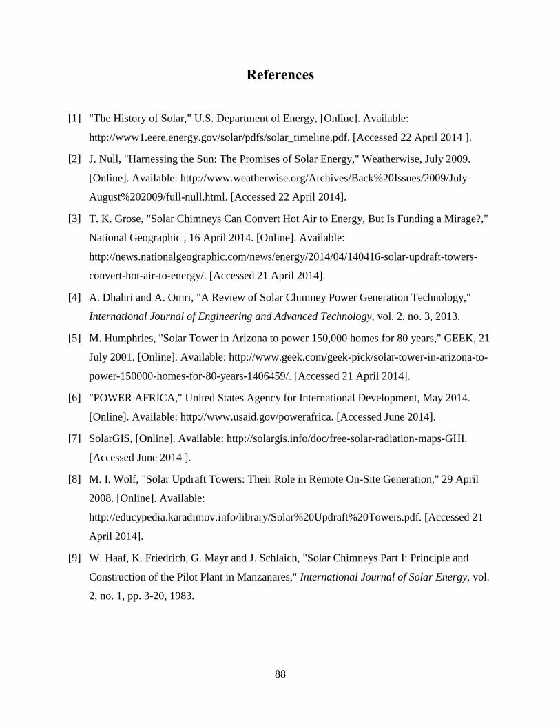
88

References

[1] "The History of Solar," U.S. Department of Energy, [Online]. Available:

http://www1.eere.energy.gov/solar/pdfs/solar_timeline.pdf. [Accessed 22 April 2014 ].

[2] J. Null, "Harnessing the Sun: The Promises of Solar Energy," Weatherwise, July 2009.

[Online]. Available: http://www.weatherwise.org/Archives/Back%20Issues/2009/July-

August%202009/full-null.html. [Accessed 22 April 2014].

[3] T. K. Grose, "Solar Chimneys Can Convert Hot Air to Energy, But Is Funding a Mirage?,"

National Geographic , 16 April 2014. [Online]. Available:

http://news.nationalgeographic.com/news/energy/2014/04/140416-solar-updraft-towers-

convert-hot-air-to-energy/. [Accessed 21 April 2014].

[4] A. Dhahri and A. Omri, "A Review of Solar Chimney Power Generation Technology,"

International Journal of Engineering and Advanced Technology, vol. 2, no. 3, 2013.

[5] M. Humphries, "Solar Tower in Arizona to power 150,000 homes for 80 years," GEEK, 21

July 2001. [Online]. Available: http://www.geek.com/geek-pick/solar-tower-in-arizona-to-

power-150000-homes-for-80-years-1406459/. [Accessed 21 April 2014].

[6] "POWER AFRICA," United States Agency for International Development, May 2014.

[Online]. Available: http://www.usaid.gov/powerafrica. [Accessed June 2014].

[7] SolarGIS, [Online]. Available: http://solargis.info/doc/free-solar-radiation-maps-GHI.

[Accessed June 2014 ].

[8] M. I. Wolf, "Solar Updraft Towers: Their Role in Remote On-Site Generation," 29 April

2008. [Online]. Available:

http://educypedia.karadimov.info/library/Solar%20Updraft%20Towers.pdf. [Accessed 21

April 2014].

[9] W. Haaf, K. Friedrich, G. Mayr and J. Schlaich, "Solar Chimneys Part I: Principle and

Construction of the Pilot Plant in Manzanares," International Journal of Solar Energy, vol.

2, no. 1, pp. 3-20, 1983.

89

[10] "Solar Chimney Manzanares," [Online]. Available: http://data.solar-

tower.org.uk/pdf/Aufwindkraftwerk_Demonstration_sanlage.pdf. [Accessed February

2014].

[11] W. Haaf, "Solar Chimneys Part II: Preliminary Test Resulats from the Manzanares Pilot

Plant," International Journal of Solar Energy, vol. 2, no. 2, pp. 141-161, 1984.

[12] H. Pastohr, O. Kornadt and G. Klaus, "Numerical and Analytical Calculations of the

Temperature Flow Field in the Upwind Power Plant," International Journal of Energy

Research, vol. 28, pp. 495-510, 2004.

[13] G. Xu, T. Ming, Y. Pan, F. Meng and C. Zhou, "Numerical Analysis of the Performance of

Solar Chimney Power Plant System," Energy Conversion and Management, no. 42, pp.

876-883, 2011.

[14] T. Ming, W. Liu, Y. Pan and G. Xu, "Numerical analysis of flow and heat transfer

characteristics in solar chimney power plants with energy storage layer," Energy

Conversion and Management, no. 49, pp. 2872-2879, 2008.

[15] P.-h. Guo, J.-y. Li and Y. Wang, "Numerical simulations of solar chimney power plant

with radiation model," Renewable Energy, no. 62, pp. 24-30, 2014.

[16] E. Gholamalizadeh and M. Kim, "Three-dimensional CFD analysis for simulating the

greenhouse effect in solar chimney power plants using a two-band radiation model,"

Renewable Energy, no. 63, pp. 498-506, 2014.

[17] H. F. Fasel, F. L. Meng, E. Shams and A. Gross, "CFD analysis for solar chimney power

plant systems," Solar Energy, pp. 12-22, 2013.

[18] T. Chergui, S. Larbi and A. Bouhdjar, "Thermo-hydrodynamic aspect analysis of flows in

solar chimney power plants-A case study," Renewable and Sustainable Energy Reviews,

no. 14, pp. 1410-1418, 2010.

[19] T. Tahar and D. Mahfoud, "Numerical Analysis of Flows in a Solar Chimney Power Plant

with a Curved Junction," International Journal of Energy Science, vol. 3, no. 4, pp. 280-

286, 2013.

[20] T. L. Bergman, A. S. Lavine, F. P. Incropera and D. P. Dewitt, Fundamentals of Heat and

Mass Transfer, Hoboken, NJ: John Wiley & Sons, INC, 2011.

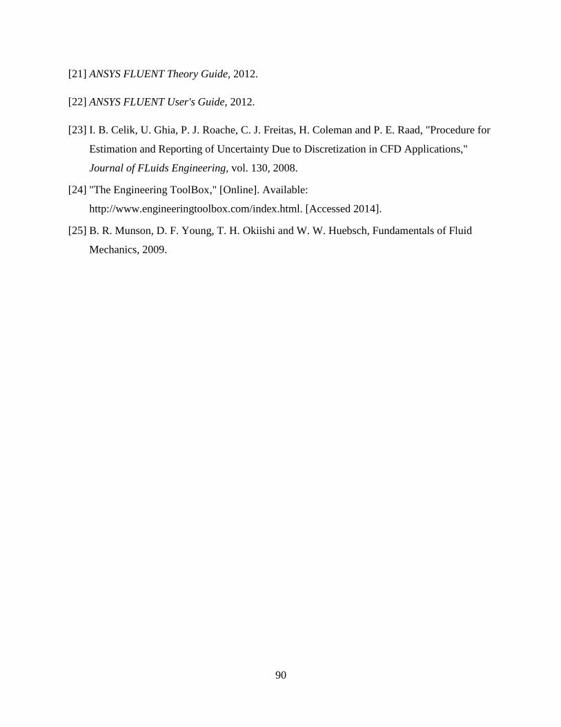
90

[21] ANSYS FLUENT Theory Guide, 2012.

[22] ANSYS FLUENT User's Guide, 2012.

[23] I. B. Celik, U. Ghia, P. J. Roache, C. J. Freitas, H. Coleman and P. E. Raad, "Procedure for

Estimation and Reporting of Uncertainty Due to Discretization in CFD Applications,"

Journal of FLuids Engineering, vol. 130, 2008.

[24] "The Engineering ToolBox," [Online]. Available:

http://www.engineeringtoolbox.com/index.html. [Accessed 2014].

[25] B. R. Munson, D. F. Young, T. H. Okiishi and W. W. Huebsch, Fundamentals of Fluid

Mechanics, 2009.