exploratory factor analysis principal components analysis ... · exploratory factor analysis (and...

Exploratory Factor Analysis (and Principal Components Analysis)

‐and‐Conducting Exploratory Analyses

with CFA (Why I Hate EFA)Advanced Multivariate Statistical

Methods Workshop

University of Georgia:

Institute for Interdisciplinary Research in Education and Human Development

11 ‐ PCA and EFA (with CFA)

Covered this Section

• Methods for exploratory factor analysis (EFA) Principal Components‐based (TERRIBLE)

Maximum Likelihood‐based Exploratory Factor Analysis (BAD)

Exploratory Structural Equation Modeling (ALSO BAD)

• Comparisons of CFA and EFA

• How to do exploratory analyses with CFA Structure of no items known

Structure of some items known

11 ‐ PCA and EFA (with CFA) 2

The Logic of Exploratory Analyses

• Exploratory analyses attempt to discover hidden structure in data with little to no user input Aside from the selection of analysis and estimation

• The results from exploratory analyses can be misleading If data do not meet assumptions of model or method selected If data have quirks that are idiosyncratic to the sample selected If some cases are extreme relative to others If constraints made by analysis are implausible

• Sometimes, exploratory analyses are needed Must construct an analysis that capitalizes on the known features of data There are better ways to conduct such analyses

• Often, exploratory analyses are not needed But are conducted anyway – see a lot of reports of scale development that

start with the idea that a construct has a certain number of dimensions


ADVANCED MATRIX OPERATIONS


A Guiding Example

• To demonstrate some advanced matrix algebra, we will make use of data

• I collected data SAT test scores for both the Math (SATM) and Verbal (SATV) sections of 1,000 students

• The descriptive statistics of this data set are given below:


Matrix Trace

• For a square matrix with p rows/columns, the trace is the sum of the diagonal elements:

• For our data, the trace of the correlation matrix is 2 For all correlation matrices, the trace is equal to the number of variables because all diagonal elements are 1

• The trace will be considered the total variance in principal components analysis Used as a target to recover when applying statistical models


Matrix Determinants

• A square matrix can be characterized by a scalar value called a determinant:

det

• Calculation of the determinant by hand is tedious Our determinant was 0.3916 Computers can have difficulties with this calculation (unstable in cases)

• The determinant is useful in statistics: Shows up in multivariate statistical distributions Is a measure of “generalized” variance of multiple variables

• If the determinant is positive, the matrix is called positive definite Is invertable

• If the determinant is not positive, the matrix is called non‐positive definite

Not invertable


Matrix Orthogonality

• A square matrix is said to be orthogonal if:

• Orthogonal matrices are characterized by two properties:1. The dot product of all row vector multiples is the zero vector

Meaning vectors are orthogonal (or uncorrelated)

2. For each row vector, the sum of all elements is one Meaning vectors are “normalized”

• The matrix above is also called orthonormal The diagonal is equal to 1 (each vector has a unit length)

• Orthonormal matrices are used in principal components and exploratory factor analysis


Eigenvalues and Eigenvectors

• A square matrix can be decomposed into a set of eigenvalues and a set of eigenvectors

• Each eigenvalue has a corresponding eigenvector The number equal to the number of rows/columns of

The eigenvectors are all orthogonal

• Principal components analysis uses eigenvalues and eigenvectors to reconfigure data


Eigenvalues and Eigenvectors Example

• In our SAT example, the two eigenvalues obtained were:

• The two eigenvectors obtained were:

• These terms will have much greater meaning in one moment (principal components analysis)


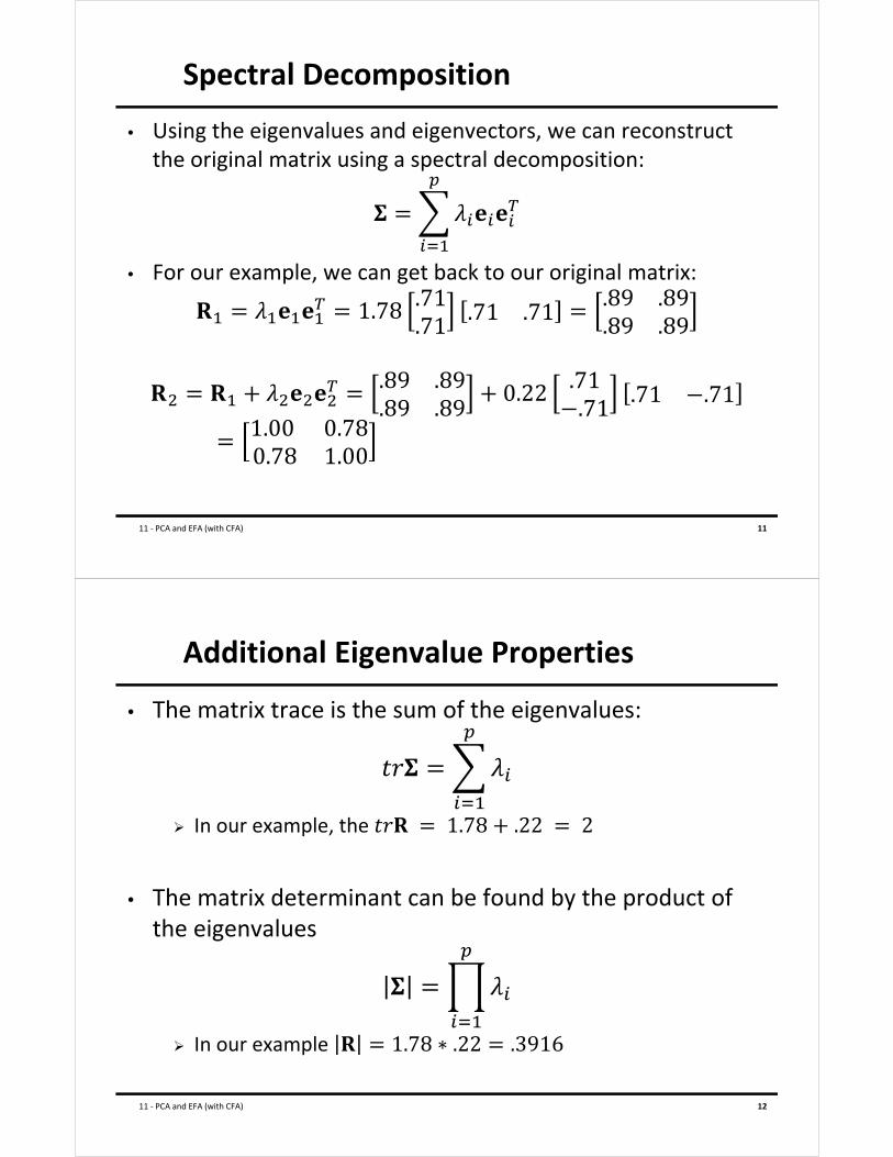
Spectral Decomposition

• Using the eigenvalues and eigenvectors, we can reconstruct the original matrix using a spectral decomposition:

• For our example, we can get back to our original matrix:


Additional Eigenvalue Properties

• The matrix trace is the sum of the eigenvalues:

In our example, the 1.78 .22 2

• The matrix determinant can be found by the product of the eigenvalues

In our example 1.78 ∗ .22 .3916


AN INTRODUCTION TO PRINCIPAL COMPONENTS ANALYSIS


PCA Overview

• Principal Components Analysis (PCA) is a method for re‐expressing the covariance (or often correlation) between a set of variables The re‐expression comes from creating a set of new variables (linear combinations) of the original variables

• PCA has two objectives:1. Data reduction

Moving from many original variables down to a few “components”

2. Interpretation Determining which original variables contribute most to thenew “components”


Goals of PCA

• The goal of PCA is to find a set of k principal components (composite variables) that: Is much smaller in number than the original set of p variables

Accounts for nearly all of the total variance Total variance = trace of covariance/correlation matrix

• If these two goals can be accomplished, then the set of kprincipal components contains almost as much information as the original p variables Meaning – the components can now replace the original variables in any subsequent analyses


Questions when using PCA

• PCA analyses proceed by seeking the answers to two questions:

1. How many components (new variables) are needed to “adequately” represent the original data? The term adequately is fuzzy (and will be in the analysis)

2. (once #1 has been answered): What does each component represent? The term “represent” is also fuzzy


PCA Features

• PCA often reveals relationships between variables that were not previously suspected New interpretations of data and variables often stem from PCA

• PCA usually serves as more of a means to an end rather than an end it itself Components (the new variables) are often used in other statistical techniques Multiple regression Cluster analysis

• Unfortunately, PCA is often intermixed with Exploratory Factor Analysis Don’t. Please don’t. Please make it stop.


PCA Details

• Notation: are our new components and is our original data matrix (with N observations and p variables) We will let i be our index for a subject

• The new components are linear combinations:

• The weights of the components come from the eigenvectors of the covariance or correlation matrix


Details About the Components

• The components are formed by the weights of the eigenvectors of the covariance or correlation matrix of the original data The variance of a component is given by the eigenvalue associated

with the eigenvector for the component

• Using the eigenvalue and eigenvectors means: Each successive component has lower variance

Var(Y1) > Var(Y2) > … > Var(Yp)

All components are uncorrelated The sum of the variances of the principal components is equal to the

total variance:


PCA on our Example

• We will now conduct a PCA on the correlation matrix of our sample data This example is given for demonstration purposes – typically we will not do PCA on small numbers of variables


PCA in SAS

• The SAS procedure that does principal components is called proc princomp Not displayed as it is not part of this course

Mplus does not compute principal components


Graphical Representation

• Plotting the components and the original data side by side reveals the nature of PCA: Shown from PCA of covariance matrix


PCA with Gambling Items

• To show how PCA works with a larger set of items, we will examine the 10 GRI items (the ones that fit the one‐factor scale)

• TO DO THIS YOU MUST IMAGINE: THESE WERE THE ONLY 10 ITEMS YOU HAD YOU WANTED TO REDUCE THE 10 ITEMS INTO 1 OR 2 COMPONENT VARIABLES

CAPITAL LETTERS ARE USED AS YOU SHOULD NEVER DO A PCA AFTER RUNNING A CFA – DIFFERENT PURPOSES!

• I will use SAS (my syntax is online), but I will not show you how as it is outside the scope of this course I will show you how to perform EFA in Mplus


Question #1: How Many Components?

• To answer the question of how many components, two methods are used: Scree plot of eigenvalues (looking for the “elbow”)

Variance accounted for (should be > 70%)

• We will go with 4 components: (VAC = 75%)

• Here VAC is for total variance (not each item as in CFA)


0

0.5

1

1.5

2

2.5

3

3.5

4

4.5

1 2 3 4 5 6 7 8 9 10

Scree Plot of Eigenvalues

0

0.1

0.2

0.3

0.4

0.5

0.6

0.7

0.8

0.9

1

1 2 3 4 5 6 7 8 9 10

Cumulative Variance Accounted For

Question #2:What Does Each Component Represent?

• To answer question #2 – we look at the weights of the eigenvectors (here is the unrotated solution)


EigenvectorsPrin1 Prin2 Prin3 Prin4

GRI1 0.31 0.10 0.17 0.84GRI3 0.23 0.08 0.18 0.13GRI5 0.32 0.09 0.23 ‐0.03GRI9 0.24 0.09 0.16 ‐0.03GRI10 0.28 0.09 0.24 ‐0.08GRI13 0.33 0.16 0.19 ‐0.22GRI14 0.45 ‐0.86 ‐0.23 ‐0.01GRI18 0.35 0.40 ‐0.83 0.03GRI21 0.27 0.14 0.06 ‐0.20GRI23 0.33 0.10 0.14 ‐0.42

Final Result: Four Principal Components

• Using the weights of the eigenvectors, we can create four new variables – the four principal components SAS does this for our standardized variables

• Each of these is uncorrelated with each other The variance of each is equal to the corresponding eigenvalue

• We would then use these in subsequent analyses


PCA Summary

• PCA is a data reduction technique that relies on the mathematical properties of eigenvalues and eigenvectors Used to create new variables (small number) out of the old data (lots of variables)

The new variables are principal components (they are not factor scores)

• PCA appeared first in the psychometric literature Many “factor analysis” methods used variants of PCA before likelihood‐based statistics were available

• Currently, PCA (or variants) methods are the default option in SPSS and SAS (proc factor)


Potentially Solvable Statistical Issues in PCA

• The typical PCA analysis also has a few statistical issues Some of these can be solved if you know what you are doing The typical analysis (using program defaults) does not solve these

• Missing data is omitted using listwise deletion – biases possible Could use ML to estimate covariance matrix, but then would have to

assume multivariate normality

• The distributions of variables can be anything…but variables with much larger variances will look like they contribute more to each component Could standardize variables – but some can’t be standardized easily (think

gender)

• The lack of standard errors makes the component weights (eigenvector elements) hard to interpret Can use a resampling/bootstrap analysis to get SEs (but not easy to do)


My (Unsovable) Issues with PCA

• My issues with PCA involve the two questions in need of answers for any use of PCA:

1. The number of components needed is not based on a statistical hypothesis test and hence is subjective Variance accounted for is a descriptive measure No statistical test for whether an additional component significantly

accounts for more variance

2. The relative meaning of each component is questionableat best and hence is subjective Typical packages provide no standard errors for each eigenvector weight

(can be obtained in bootstrap analyses) No definitive answer for component composition

• In sum, I feel it is very easy to be mislead (or purposefully mislead) with PCA


EXPLORATORY FACTOR ANALYSIS


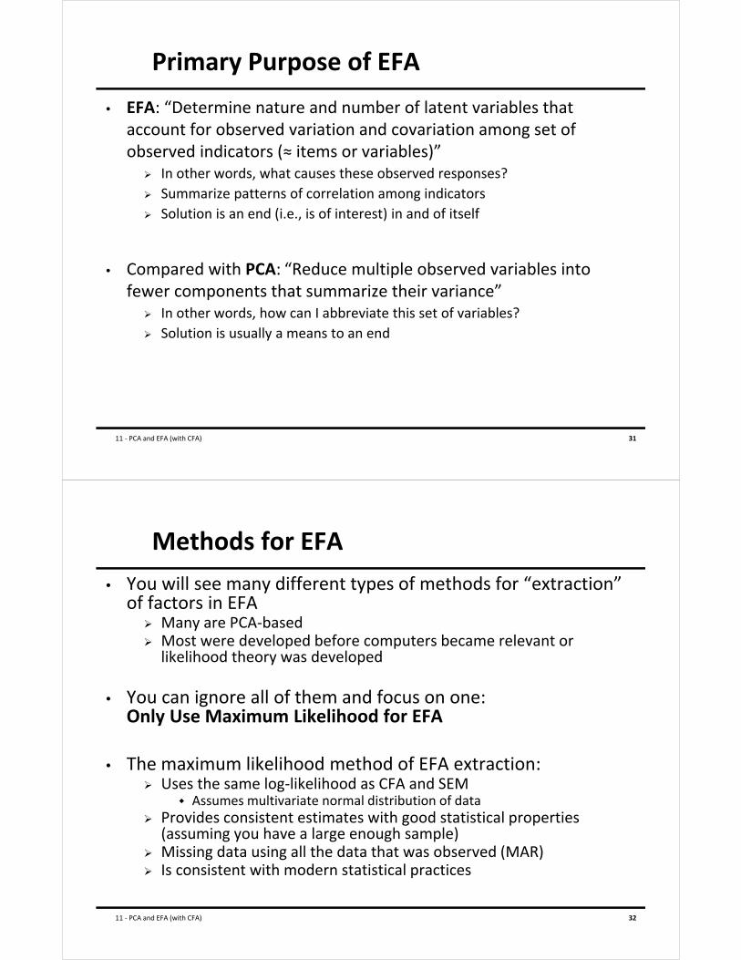
Primary Purpose of EFA

• EFA: “Determine nature and number of latent variables that account for observed variation and covariation among set of observed indicators (≈ items or variables)” In other words, what causes these observed responses?

Summarize patterns of correlation among indicators

Solution is an end (i.e., is of interest) in and of itself

• Compared with PCA: “Reduce multiple observed variables into fewer components that summarize their variance” In other words, how can I abbreviate this set of variables?

Solution is usually a means to an end


Methods for EFA

• You will see many different types of methods for “extraction” of factors in EFA Many are PCA‐based Most were developed before computers became relevant or

likelihood theory was developed

• You can ignore all of them and focus on one: Only Use Maximum Likelihood for EFA

• The maximum likelihood method of EFA extraction: Uses the same log‐likelihood as CFA and SEM

Assumes multivariate normal distribution of data Provides consistent estimates with good statistical properties

(assuming you have a large enough sample) Missing data using all the data that was observed (MAR) Is consistent with modern statistical practices


Questions when using EFA

• EFAs proceed by seeking the answers to two questions:

(the same questions posed in PCA; but with different terms)

1. How many latent factors are needed to “adequately” represent the original data? “Adequately” = does a given EFA model fit well?

2. (once #1 has been answered): What does each factor represent? The term “represent” is fuzzy


How Maximum Likelihood EFA Works

• Maximum likelihood EFA assumes the data follow a multivariate normal distribution The basis for the log‐likelihood function (same log‐likelihood we have used in every analysis to this point)

• The log‐likelihood function depends on two sets of parameters: the mean vector and the covariance matrix Mean vector is saturated (just uses the item means for item intercepts) – so it is often not thought of in analysis Denoted as

Covariance matrix is what gives “factor structure” EFA models provide a structure for the covariance matrix


The EFA Model for the Covariance Matrix

• The covariance matrix is modeled based on how it would look if a set of hypothetical (latent) factors had caused the data

• For an analysis measuring factors, each item in the EFA: Has 1 unique variance parameter

Has factor loadings

• The initial estimation of factor loadings is conducted based on the assumption of uncorrelated factors Assumption is dubious at best –yet is the cornerstone of the analysis


Model Implied Covariance Matrix

• Recall from CFA that the factor model implied covariance matrix is Where:

= model implied covariance matrix of the observed data (size x )

= matrix of factor loadings (size x )– In EFA: all terms in are estimated

= factor covariance matrix (size x )– In EFA: (all factors have variances of 1 and covariances of 0)

= matrix of unique (residual) variances (size x )– In EFA: is diagonal by default (no residual covariances)

• Therefore, the EFA model‐implied covariance matrix is:


EFA Model Identifiability

• Under the ML method for EFA, the same rules of identification apply to EFA as to CFA/Path Analysis T‐rule: Total number of EFA model parameters must not exceed unique elements in saturated covariance matrix of data For an analysis with a number of factors and a set number of items there are ∗ 1 EFA model parameters

As we will see, there must be constraints for the model to work

Therefore, 1

Local‐identification: each portion of the model must be locally identified With all factor loadings estimated local identification fails

– No way of differentiating factors without constraints


Constraints to Make EFA in ML Identified

• The EFA model imposes the following constraint:

such that is a diagonal matrix

• This puts constraints on the model (that many fewer parameters to estimate)

• This constraint is not well known – and how it functions is hard to describe For a 1‐factor model, the results of EFA and CFA will match

• Note: the other methods of EFA “extraction” avoid this constraint by not being statistical models in the first place

PCA‐based routines rely on matrix properties to resolve identification


The Nature of the Constraints in EFA

• The EFA constraints provide some detailed assumptions about the nature of the factor model and how it pertains to the data

• For example, take a 2‐factor model (one constraint):

0

• In short, some combinations of factor loadings and unique variances (across and within items) cannot happen This goes against most of our statistical constraints – which must be

justifiable and understandable (therefore testable)

This constraint is not testable in CFA


The Log‐Likelihood Function

• Given the model parameters, the EFA model is estimated by maximizing the multivariate normal log‐likelihood For the data

log log 2 exp2

2log 2

2log

2

• Under EFA, this becomes:


Benefits and Consequences of EFA with ML

• The parameters of the EFA model under ML retain the same benefits and consequences of any model (i.e., CFA) Asymptotically (large N) they are consistent, normal, and efficient Missing data are “skipped” in the likelihood, allowing for incomplete

observations to contribute (assumed MAR)

• Furthermore, the same types of model fit indices are available in EFA as are in CFA

• As with CFA, though, an EFA model must be a close approximation to the saturated model covariance matrix if the parameters are to be believed This is a marked difference between EFA in ML and EFA with other

methods – quality of fit is statistically rigorous


FACTOR LOADING ROTATIONS IN EFA


Rotations of Factor Loadings in EFA

• Transformations of the factor loadings are possible as the matrix of factor loadings is only unique up to an orthogonal transformation Don’t like the solution? Rotate!

• Historically, rotations use the properties of matrix algebra to adjust the factor loadings to more interpretable numbers

• Modern versions of rotations/transformations rely on “target functions” that specify what a “good” solution should look like The details of the modern approach are lacking in most texts


Types of Classical Rotated Solutions

• Multiple types of rotations exist but two broad categories seem to dominate how they are discussed:

• Orthogonal rotations: rotations that force the factor correlation to zero (orthogonal factors). The name orthogonal relates to the angle between axes of factor solutions being 90 degrees. The most prevalent is the varimax rotation.

• Oblique rotations: rotations that allow for non‐zero factor correlations. The name orthogonal relates to the angle between axes of factor solutions not being 90 degrees. The most prevalent is the promax rotation. These rotations provide an estimate of “factor correlation”


How Classical Orthogonal Rotation Works

• Classical orthogonal rotation algorithms work by defining a new rotated set of factor loadings ∗ as a function of the original (non‐rotated) loadings and an orthogonal rotation matrix

∗

where:

• These rotations do not alter the fit of the model as∗ ∗


Modern Versions of Rotation

• Most studies using EFA use the classical rotation mechanisms, likely due to insufficient training

• Modern methods for rotations rely on the use of a target function for how an optimal loading solution should look


From Browne (2001)

Rotation Algorithms

• Given a target function, rotation algorithms seek to find a rotated solution that simultaneously:

1. Minimizes the distance between the rotated solution and the original factor loadings

2. Fits best to the target function

• Rotation algorithms are typically iterative – meaning they can fail to converge

• Rotation searches typically have multiple optimal values Need many restarts


EFA IN MPLUS


EFA in Mplus

• Mplus has an extensive set of rotation algorithms The default is the Geomin rotation procedure

• The Geomin procedure is the default as it was shown to have a good performance for a classic Thurstone data set (see Browne, 2001)

• We could spend an entire semester on rotations, so I will focus on the default option in Mplus and let the results generalize across most methods


Steps in an ML EFA Analysis

• To determine number of factors:1. Run a 1‐factor model (note: same fit as CFA model)

Check model fit (RMSEA, CFI, TLI) – stop if model fits adequately

2. Run a 2‐factor model Check model fit (RMSEA, CFI, TLI) – stop if model fits adequately

3. Run a 3‐factor model (if possible – remember maximum number of parameters possible) Check model fit (RMSEA, CFI, TLI) – stop if model fits adequately

And so on…

• One huge note: unlike in PCA analyses, there are no model‐based eigenvalues to report (nor VAC for the whole model) These are no longer useful in determining the number of factors Mplus will give you a plot (PLOT command, TYPE=PLOT2)

These are from the H1 model correlation matrix


10 Item GRI: EFA Using ML in Mplus

• The 10 item GRI has a unique parameters in

the H1 (saturated) covariance matrix The limit of parameters possible in an EFA model

In theory, we could estimate 6 factors In practice, 6 factors is impossible with 10 items


Factors Factor Loadings

Unique Variances

Constraints Total Covariance Parameters

1 10 10 0 20

2 20 10 1 29

3 30 10 3 37

4 40 10 6 46

5 50 10 10 50

6 60 10 15 55

Mplus Syntax


Model Comparison: Fit Statistics

F Log‐Likelihood #Ptrs AIC BIC SSA BIC RMSEA CFI TLI

1 ‐16,648.054 30 33,356.108 33,512.031 33,416.735 .052 .969 .961

2 ‐16,595.511 39 33,269.021 33,471.721 33,347.835 .029 .993 .987

3 ‐16,581.715 47 33,257.431 33,501.710 33,352.412 .021 .997 .994

4 ‐16.572.437 54 33,252.873 33,533.535 33,362.001 .000 1.000 1.001

5 ‐16,568.963 60 33,257.925 33,569.771 33,379.178 .000 1.000 1.004

6 ‐16.567.438 65 33,264.875 33,602.709 33,396.232 .000 1.000 1.000


Model Comparison: Likelihood Ratio Tests

• Model 1 v. Model 2:




• Likelihood ratio tests suggest a 4‐factor solution However, RMSEA, CFI, and TLI all would be acceptable under one factor


Mplus Output: A New Warning

• A new warning now appears in the Mplus output:

• The GEOMIN rotation procedure uses an iterative algorithm that attempts to provide a good fit to the non‐rotated factor loadings while minimizing a penalty function It may not converge It may converge to a local minimum It may converge to a location that is not well identified (as is our

problem)

• Upon looking at our 4‐factor results, we find some very strange numbers So we will stick to the 3‐factor model for our explanation In reality you shouldn’t do this (but you shouldn’t do EFA)


Mplus EFA 3‐Factor Model Output

• The key to interpreting EFA output is the factor loadings:

• Historically, the standard has been if the factor loading is bigger than .3, then the item is considered to load onto the factor This is different under ML – as we can now use Wald tests


Wald Tests for Factor Loadings

• Using the Wald Tests, we see a different story (absolute value must be great than 2 to be significant)

• Factor 2 has 1 item that significantly loads onto it

• Factor 3 has 4 items

• Factor 1 has 4 items

• Two items have no significant loadings at all


Factor Correlations

• Another salient feature in oblique rotations is that of the factor correlations

• Sometimes these values can exceed 1 (called factor collapse) so it is important to check


Where to Go From Here

• If this was your analysis, you would have to make a determination as to the number of factors We thought 4 – but 4 didn’t work

Then we thought 3 – but the solution for 3 wasn’t great

Can anyone say 2?

• Once you have settled the number of factors, you must then describe what each factor means Using the pattern of rotated loadings

• After all that, you should validate your result You should regardless of analysis (but especially in EFA)


PCA VERSUS EFA


EFA vs. PCA

• 2 very different schools of thought on exploratory factor analysis (EFA) vs. principal components analysis (PCA):1. EFA and PCA are TWO ENTIRELY DIFFERENT THINGS…

2. PCA is a special kind (or extraction type) of EFA… although they are often used for different purposes, the results turn out the same a lot anyway, so what’s the big deal?

• My world view: I’ll describe them via school of thought #2

I want you to know what their limitations areI want you to know that they are not really testable models

It is not your data’s job to tell you what constructs you are measuring!! If you don’t have any idea, game over


PCA vs. EFA, continued

• So if the difference between EFA and PCA is just in the communalities (the diagonal of the correlation matrix)… PCA: All variance in indicators is analyzed

No separation of common variance from error variance

Yields components that are uncorrelated to begin with

EFA: Only common variance in indicators is analyzed Separates common variance from error variance

Yields factors that may be uncorrelated or correlated

• Why the controversy? Why is EFA considered to be about underlying structure, while PCA is supposed to be used only for data reduction?

The answer lies in the theoretical model underlying each…


Big Conceptual Difference between PCA and EFA

• In PCA, we get components that are outcomes built from linear combinations of the indicators: C1 = L11I1 + L12I2 + L13I3 + L14I4 + L15I5 C2 = L21I1 + L22I2 + L23I3 + L24I4 + L25I5 … and so forth – note that C is the OUTCOME

This is not a testable measurement model by itself.

• In EFA, we get factors that are thought to be the cause of the observed indicators (here, 5 indicators, 2 factors): I1 = L11F1 + L12F2 + e1 I2 = L21F1 + L22F2 + e1 I3 = L31F1 + L32F2 + e1 … and so forth… but note that F is the PREDICTOR testable


PCA vs. EFA/CFA

Factor

Y1 Y2 Y3 Y4

e1 e2 e3 e4

Component

Y1 Y2 Y3 Y4

This is not a testable measurement model, because how do we know if we’ve combined stuff “correctly”?

This IS a testable measurement model, because we are trying to predict the observed covariances between the indicators by creating a factor – the factor IS the reason for the covariance.


Big Conceptual Difference between PCA and EFA

• In PCA, the component is just the sum of the parts, and there is no inherent reason why the parts should be correlated (they just are)

But they should be (otherwise, there’s no point in trying to build components to summarize the variables “component” = “variable”)

The type of construct measured by a component is often called an ‘emergent’ construct – i.e., it emerges from the indicators (“formative”).

Examples: “Lack of Free time”, “SES”, “Support/Resources”

• In EFA, the indicator responses are caused by the factors, and thus should be uncorrelated once controlling for the factor(s)

The type of construct that is measured by a factor is often called a ‘reflective’ construct – i.e., the indicators are a reflection of your status on the latent variable.

Examples: Pretty much everything else…


My Issues with EFA

• Often a PCA is done and called an EFA PCA is not a statistical model!

• No statistical test for factor adequacy

• Rotations are suspect

• Constraints are problematic


COMPARING CFA AND EFA


Comparing CFA and EFA

• Although CFA and EFA are very similar, their results can be very different for two or more factors Results for the 1 factor are the same in both (use standardized factor identification in CFA)

• EFA typically assumes uncorrelated factors

• If we fix our factor correlation to zero, a CFA model becomes very similar to an EFA model But…with one exception…


EFA Model Constraints

• For more than one factor, the EFA model has too many parameters to estimate Uses identification constraints (where is diagonal):

• This puts multivariate constraints on the model

• These constraints render the comparison of EFA and CFA useless for most purposes Many CFA models do not have these constraints

• Under maximum likelihood estimators, both EFA and CFA use the same likelihood function Multivariate normal Mplus: full information


CFA Approaches to EFA

• We can conduct exploratory analysis using a CFA model Need to set the right number of constraints for identification We set the value of factor loadings for a few items on a few of the factors Typically to zero (my usual thought) Sometimes to one (Brown, 2002)

We keep the factor covariance matrix as an identity Uncorrelated factors (as in EFA) with variances of one

• Benefits of using CFA for exploratory analyses: CFA constraints remove rotational indeterminacy of factor loadings – no rotating is needed (or possible)

Defines factors with potentially less ambiguity Constraints are easy to see

For some software (SAS and SPSS), we get much more model fit information


EFA with CFA Constraints

• To do EFA with CFA, you must: Fix factor loadings (set to either zero or one)

Use “row echelon” form :

One item has only one factor loading estimated

One item has only two factor loadings estimated

One item has only three factor loadings estimated

Fix factor covariances Set all to 0

Fix factor variances Set all to 1


Re‐Examining Our EFA of GRI 10 Items

• We will fit a series of “just‐identified” CFA models and examine our results

• NOTE: the one factor model CFA model will be identical to the one factor EFA model The loadings and unique variances in the EFA model are the standardized versions from the CFA model


Model Comparison


F Log‐Likelihood #Ptrs AIC BIC SSA BIC RMSEA CFI TLI

1 ‐16,648.054 30 33,356.108 33,512.031 33,416.735 .052 .969 .961

2 ‐16,595.511 39 33,269.021 33,471.721 33,347.835 .029 .993 .987

3 ‐16,581.715 47 33,257.431 33,501.710 33,352.412 .021 .997 .994

4 Did not converge

5 Did not converge

6 Did not converge

Three Factor Model Results

• As no model beyond the 3‐factor model worked, we are left to look at the 3‐factor model results Note: all model fit identically to the EFA model counterparts

• The factor loadings showed an interesting pattern ‐ no items had significant loadings onto factors 2 or 3

• As such, the 3‐factor model is difficult to defend


CONCLUDING REMARKS


Wrapping Up

• We discussed the world of exploratory factor analysis and found the following: PCA is what people typically run when they are after EFA

ML EFA is a better option to pick (likelihood based) Constraints employed are hidden!

Rotations can break without you realizing they do

ML EFA can be shown to be equal to CFA for certain models

Overall, CFA is still your best bet


exploratory factor analysis principal components analysis ... · exploratory factor analysis (and...

Documents