exploration of electrospinning methods for fabricating
TRANSCRIPT

1
Exploration of Electrospinning
Methods for Fabricating Synthetic
Human Knee Ligaments
Aleksia Pilja
Supervised by Dr Saulo Martelli
Submitted to Flinders University
College of Science and Engineering
Master of Engineering (Biomedical)
October 2019

2
Abstract The ligaments of the knee are crucial in providing particular movement limitations and overall
stability to the joint. Cruciate ligaments maintain anteroposterior, rotational and one-plane medial
or lateral stability in conjunction with the collateral structures [41]. Rupture to any of the
supportive structures disrupts the kinematics of the femoral-tibial joint, causing functional
impairment in the initial trauma [39]. In the majority of cases, surgical intervention is required to
repair the initial function, however replacement grafts often lack the mechanical properties of the
original ligament. Disruption in the stability of the knee eventually causes long-term effects, many
associated with early onset osteoarthritis [39]. Investigations into developing a more suitable
replacement graft is on the incline, with aims to reduce the occurrence of long-term effects. This
study focuses on the development of synthetic ligaments through electrospinning means, with key
objectives in replicating the elastic modulus of native knee ligaments. For the anterior cruciate
ligament (ACL), the elastic modulus was found to be between 65 and 128 MPa [13,14].
The process of electrospinning involves the development and collection of small-scale fibres, with
aims to replicate the fibrous nature of native ligaments. Fibre formation was achieved in the
electrospinning device by passing a polymer solution through a high electric field and onto a
rotating drum collector. The solutions tested consisted of numerous concentrations of
polycaprolactone (PCL) in ratios of chloroform and dimethylformamide (DMF). The fibre stream
formed in the process is highly governed by the electrospinning parameters used during
experiments. Although influenced by all contributing factors, the fibre morphology was highly
dependent on the flow rate of the solution, the applied voltage and the rotational speed of the
collecting drum. The solution flow rate was typically set to 1.5 mL/h, while the applied voltage and
rotational speed of the collector varied between 20-30 kV and 1000 to 1500 rpm, respectively. After
the two-hour test duration, fibre sheets were rolled into a cylindrical bundle structures for
mechanical testing. Tensile testing of samples was conducted at a 30% per second strain rate, where
resultant data was used to produce stress-strain curves and calculate the elastic modulus of the
samples. The unrolled fibres were viewed using a scanning electron microscope (SEM), in order to
determine the resulting fibre morphology from the test conditions.
Upon testing, it was found that the 13% w/v PCL concentration solutions produced synthetic
ligament samples with desirable mechanical properties. The elastic modulus for these samples was
found to be between 69 and 106 MPa (n=8). Although exact fibre alignment was not achieved, an
eventual recruitment of fibres under increasing tension was displayed in the stress-strain curves for
particular samples. The smallest fibres were seen in the 10% solutions (198 – 366 nm), with
diameters within the fibril range of a native ligament. The 13% solutions however, produced larger
fibres (0.4 – 2 µm), placing them in the collagen fibre range of native ligaments [23]. Results indicate
that a desirable elastic modulus can be achieved in the synthetic electrospun ligaments with the use
of 13% w/v PCL solutions and the correct combination of electrospinning parameters.

3
Declaration I certify that this thesis:
1. Does not incorporate without acknowledgement any material previously submitted for a degree or
diploma in any university; and
2. 2. To the best of my knowledge and belief, does not contain any material previously published or
written by another person except where due reference is made in the text.
Aleksia Pilja, 13/2/2020

4
Acknowledgements A great expression of gratitude to Dr Saulo Martelli for the structure and the ongoing guidance
throughout the duration of the project. Many thanks also go to Dr Youhong Tang and Samaneh
Mirzaei for laboratory and electrospinning inductions. Much appreciation would also like to be
given to Michael Russo for assistance in mechanical testing. Also, many thanks to Aoife McFadden
for SEM imaging training and the assistance in sample preparation.

5
Contents Abstract ........................................................................................................................................................... 2
Declaration ...................................................................................................................................................... 3
Acknowledgements ........................................................................................................................................ 4
List of Figures .................................................................................................................................................. 7
List of Tables ................................................................................................................................................... 8
List of Equations ............................................................................................................................................. 8
1. Introduction ................................................................................................................................................ 9
2. Literature Review ..................................................................................................................................... 10
2.1 Description of the Problem ................................................................................................................ 10
2.2 Current Solutions and Limitations .................................................................................................... 11
2.3 Synthetic Electrospun Ligaments ...................................................................................................... 12
2.4 Electrospinning Background .............................................................................................................. 13
2.5 Parameter Impact on Fibres ............................................................................................................... 14
2.6 Mechanical Properties ........................................................................................................................ 16
2.7 Research Variations ............................................................................................................................ 17
2.8 Overview of Proposed Study.............................................................................................................. 21
2.8.1 Aim ............................................................................................................................................... 21
2.8.2 Objectives .................................................................................................................................... 22
2.8.3 Justifications of Decisions ......................................................................................................... 22
2.8.4 Overview of Experimental Method ......................................................................................... 22
3. Methodology ............................................................................................................................................. 23
3.1 Solution Preparation ........................................................................................................................... 23
3.2 Electrospinning Procedure ................................................................................................................. 24
3.3 Mechanical Testing ............................................................................................................................. 30
3.4 Normalising Data ................................................................................................................................ 33
3.5 SEM Imaging Method ......................................................................................................................... 34
4. Results ....................................................................................................................................................... 36
4.1 Electrospinning Outcomes ................................................................................................................. 36
4.2 Material Properties of Ligament Samples .......................................................................................... 37
4.3 Fibre Morphology ............................................................................................................................... 45
5.Discussion .................................................................................................................................................. 54
5.1 Key Findings ....................................................................................................................................... 54
5.1 Polymer Concentrations and Solution Preparation .......................................................................... 54

6
5.2 Electrospinning Procedure and Outcome ......................................................................................... 55
5.3 Potential Sources of Error .................................................................................................................. 55
5.4 Mechanical Testing ............................................................................................................................. 57
5.5 SEM Imaging ....................................................................................................................................... 58
5.6 Future Studies ..................................................................................................................................... 58
5.6.1 Project Continuation .................................................................................................................. 58
5.6.2 Further Research ........................................................................................................................ 58
6. Conclusion ................................................................................................................................................ 59
7. References ................................................................................................................................................. 59
8. Appendices ................................................................................................................................................ 62
Appendix A – Round One Stress-Strain Graphs ..................................................................................... 62
Appendix B - Round Two Stress-Strain Graph ....................................................................................... 68
Appendix C - Round Three Stress-Strain Graphs ................................................................................... 73
Appendix D – MATLAB Code for Graph Generation ............................................................................ 76
Appendix E – MATLAB Code for Correlation Graphs ........................................................................... 76

7
List of Figures FIGURE 1 - LIGAMENTS OF THE KNEE [26] ........................................................................................................................ 9
FIGURE 2 - ACL RECONSTRUCTION WITH PATELLAR TENDON REPLACEMENT [37] .................................................................... 9 FIGURE 3- HIERARCHICAL STRUCTURE OF TENDON/LIGAMENT [23] .................................................................................... 11 FIGURE 4 - TYPICAL STRESS-STRAIN RESPONSE FOR COLLAGEN FIBRES IN LIGAMENTS [20] ...................................................... 12 FIGURE 5 - SOLUTION IMPACT WITH INCREASE IN VOLTAGE, TAYLOR CONE FORMATION AT C [24] ........................................... 13 FIGURE 6 - TYPICAL ELECTROSPINNING SETUP [25] .......................................................................................................... 13 FIGURE 7 - METHOD FOR ALIGNED FIBRE BUNDLE COLLECTION [27] ................................................................................... 15 FIGURE 8 - SYRINGE PUMP AND FLOW RATE CONTROL ..................................................................................................... 24 FIGURE 9 - ROTATING MANDREL COLLECTOR COVERED IN BAKING PAPER ............................................................................ 25 FIGURE 10 – NEU-PRO ELECTROSPINNING UNIT ............................................................................................................. 25 FIGURE 11 - A) SHORT FIBRE STREAM B) LONG FIBRE JET ................................................................................................. 26 FIGURE 12 - A) LONG FIBRE STREAM B) SHORTER, FINER FIBRE JET .................................................................................... 27 FIGURE 13 - REMOVED BAKING PAPER WITH FIBRE SHEET ................................................................................................. 28 FIGURE 14 - ROLLED-UP FIBRE SHEET INTO LIGAMENT SAMPLE .......................................................................................... 28 FIGURE 15 - TEST RESOURCES DEVICE FOR TENSILE TESTING .............................................................................................. 30 FIGURE 16 - A) INCREASED STRAIN PRIOR TO B) INCREMENTAL BREAKING C) INCREASED STRAIN PRIOR TO D) CLAMP BREAKING ...... 31 FIGURE 17 – A) LOOPED END SAMPLE PRIOR TO TESTING B) LOOPED END SAMPLES DURING TESTING ......................................... 32 FIGURE 18 - SAMPLES POST SPUTTER COATING ................................................................................................................ 34 FIGURE 19 - A) SEM WITH OPEN CHAMBER B) SAMPLES PLACED ON CHAMBER STAGE PRIOR TO IMAGING .................................. 34 FIGURE 20 - STRESS-STRAIN GRAPH OF SAMPLE L6 ........................................................................................................... 36 FIGURE 21 - STRESS-STRAIN CURVE FOR SAMPLE L12 ....................................................................................................... 37 FIGURE 22 - STRESS-STRAIN CURVE FOR SAMPLE L9 ......................................................................................................... 37 FIGURE 23 - STRESS-STRAIN CURVE OF SAMPLE L32 ......................................................................................................... 38 FIGURE 24 - STRESS-STRAIN CURVE OF SAMPLE L34 ......................................................................................................... 39 FIGURE 25 - RELATIONSHIP BETWEEN PCL CONCENTRATION IN SOLUTIONS AND ELASTIC MODULUS ........................................... 40 FIGURE 26 - STRESS-STRAIN CURVE FOR SAMPLE L26 ....................................................................................................... 41 FIGURE 27 - STRESS-STRAIN CURVE FOR SAMPLE L33 ....................................................................................................... 43 FIGURE 28 - A) SAMPLE L19/L20 AT 2000X MAGNIFICATION B) SAMPLE L29/30 AT 1000X MAGNIFICATION ........................... 44 FIGURE 29 - A) SAMPLE L19/20 B) SAMPLE L21/22 C) SAMPLE L23/24 D) SAMPLE L25/26 E) SAMPLE L27/28 F) SAMPLE
L29/30 .......................................................................................................................................................... 45 FIGURE 30 - CORRELATION GRAPHS FOR 10% SOLUTION FIBRE DIAMETERS AGAINST VOLTAGE AND FINAL RPM ............................ 47 FIGURE 31 - SAMPLE L31/32 AT A) 1500 MAGNIFICATION AND B) 600X MAGNIFICATION ..................................................... 48 FIGURE 32 - SAMPLE L33/34 AT A) 2500X MAGNIFICATION AND B) 600X MAGNIFICATION .................................................... 48 FIGURE 33 - SAMPLE L35/36 AT A) 1300X MAGNIFICATION AND B) 700X MAGNIFICATION .................................................... 49 FIGURE 34 - SAMPLE L37/38 AT A) 2500X MAGNIFICATION AND B) 600X MAGNIFICATION .................................................... 49 FIGURE 35 - A) L31/32 B) L33/34 C) L35/36 D) L37/38 .............................................................................................. 50 FIGURE 36 - CORRELATION GRAPHS FOR 13% SOLUTION FIBRE DIAMETERS AGAINST VOLTAGE AND FINAL RPM ............................ 51

8
List of Tables TABLE 1 - STIFFNESS AND ELASTIC MODULUS RANGE OF NATIVE ACL ................................................................................. 15 TABLE 2 - STIFFNESS RANGES FOR NATIVE PCL, MCL, LCL ............................................................................................... 16 TABLE 3 - STIFFNESS RANGE SUMMARY OF ALL KNEE LIGAMENTS ....................................................................................... 16 TABLE 4 - ELECTROSPINNING EXPERIMENTS WITH KEY PARAMETERS .................................................................................... 18 TABLE 5 - ELECTROSPINNING EXPERIMENTS RESULT SUMMARY .......................................................................................... 19 TABLE 6 - TOP SELECTION ELECTROSPINNING EXPERIMENTS ............................................................................................... 20 TABLE 7 - SOLVENT RATIOS ......................................................................................................................................... 23 TABLE 8 - ROUND ONE ELECTROSPINNING TEST PARAMETERS ............................................................................................ 35 TABLE 9 - ROUND TWO ELECTROSPINNING TEST PARAMETERS ........................................................................................... 35 TABLE 10 - ROUND THREE ELECTROSPINNING TEST PARAMETERS ....................................................................................... 36 TABLE 11 - ROUND ONE LIGAMENT SAMPLE MEASUREMENTS AND PROPERTIES ................................................................... 40 TABLE 12 - ROUND TWO LIGAMENT SAMPLE MEASUREMENTS AND PROPERTIES ................................................................... 41 TABLE 13 - ROUND THREE LIGAMENT SAMPLES MEASUREMENTS AND PROPERTIES ............................................................... 42 TABLE 14 - SUMMARY OF VOLTAGE AND COLLECTOR RPM IN COMPARISON TO AVERAGE FIBRE DIAMETER AND PORE SIZE FOR 10%
SOLUTIONS ...................................................................................................................................................... 46 TABLE 15 - SUMMARY OF VOLTAGE AND COLLECTOR RPM IN COMPARISON TO AVERAGE FIBRE DIAMETER AND PORE SIZE FOR 13%
SOLUTIONS ...................................................................................................................................................... 50
List of Equations 𝐸𝑞𝑢𝑎𝑡𝑖𝑜𝑛 1− 𝑉𝑜𝑙𝑢𝑚𝑒 𝐹𝑟𝑎𝑐𝑡𝑖𝑜𝑛 ........................................................................................................................ 32 𝐸𝑞𝑢𝑎𝑡𝑖𝑜𝑛 2− 𝑆𝑡𝑟𝑒𝑠𝑠 ........................................................................................................................................... 33 𝐸𝑞𝑢𝑎𝑡𝑖𝑜𝑛 3− 𝑆𝑡𝑟𝑎𝑖𝑛 ........................................................................................................................................... 33 𝐸𝑞𝑢𝑎𝑡𝑖𝑜𝑛 4− 𝑌𝑜𝑢𝑛𝑔′𝑠 𝑀𝑜𝑑𝑢𝑙𝑢𝑠 ....................................................................................................................... 33 𝐸𝑞𝑢𝑎𝑡𝑖𝑜𝑛 5− 𝑆𝑐𝑎𝑙𝑖𝑛𝑔 𝐹𝑜𝑟𝑐𝑒.............................................................................................................................. 43

9
1. Introduction The progressive nature of the biomedical field can be seen in the ever-evolving research and
development of synthetic biological replacements. With focus on synthetic knee ligament
replacements, it has been recognised that improvement in surgical substitutions is required in order
to limit variation from the original ligament of concern. Surgical intervention is recommended in
the case of ligament rupture, particularly for anterior cruciate ligaments (ACL), in order to regain
knee function [34]. Even with surgical reconstruction of the ACL, 10 to 25% of patients experience
unsatisfactory results 7 to 10 years following the procedure, indicating further investigation
regarding ligament function and replacement is required [35].
Current autograft and allograft replacements offer a sound biocompatibility, yet the material and
structural behaviour in comparison to the original native ligament is often misaligned [30]. There
is value in ensuring the replacement graft has a better suited stiffness. The mismatch in desired
replacement properties can often lead to negative long-term effects due to abnormal knee
kinematics, potentially causing early onset osteoarthritis [32]. This issue can arise as a result of the
replacement altering the overall mechanics of the knee, inducing uneven force distribution across
the articular cartilage [33]. Existing synthetic replacements are not often recommended due to high
patient failure rates and potential of re-rupture [36].
An emerging method for synthetic ligament developing is electrospinning through the production
and collection of nanofibers. Manipulation of a polymer solution can be done in a high electric field
in order to achieve high-speed fibre jet production. The concept of fibre development is highly
desirable in this application since ligaments exhibit a hierarchical structure made of fibril, fibre and
fascicle layers [23]. Much research is being conducted to determine which materials,
electrospinning parameter combinations and collection methods are best suited for efficient and
desirable synthetic ligament development. There is however, a variation in key aims and what
aspect deems the synthetic ligaments as suitable for replacement.
While many studies take part in mechanical testing, few place objectives on replicating the elastic
modulus of the synthetic models to the range seen in native ligaments. This study however, sets the
primary objective as developing electrospun fibre bundles which match the desired elastic modulus
range (65 – 128 MPa), for the anterior cruciate ligament [13,14]. This mechanical evaluation is
achieved through tensile testing of the synthetic ligament fibre bundles, assessing the material
properties and response under increased load and strain. Calculating the stress and strain
experienced by each sample allows for corresponding graphs to be drawn, interpreting and
determining the elastic response within the linear region of the graphs.
Furthering material evaluation, the fibres are viewed using a scanning electron microscope (SEM).
This imaging technique allows for the analysis of fibre diameters due to great deals of magnification.
The fibre diameters are valuable to correlate which electrospinning parameters impact the fibre
production and the overall nature of the fibre material. There is also benefit is determining which
segment of the ligament hierarchical structure matches to the sizes of the synthetic samples
produced.

10
2. Literature Review2.1 Description of the Problem Knee ligament injuries have become an increased issue, with an estimation of 2 in every 1000 people
per year experiencing this issue [35], with a particular occurrence in athletes. These injuries primary
involve the anterior cruciate ligament (ACL) and the medial collateral ligament (MCL), accounting
for 90% of all sport-related injuries [35]. There have also been studies surrounding the greater risk
females experience in regards to ACL injures, with occurrence at 2 to 8 times greater than their
male counterparts [35]. Although the ACL and MCL account for the greatest amount of this injury
type, the lateral collateral ligament (LCL) and the posterior cruciate ligament (PCL) are also capable
of rupture. Traditionally, knee ligament reconstruction surgeries involve the complete removal of
the ruptured ligament and a replacement achieved from the use of an autograft, allograft or
synthetic graft. For ACL reconstruction surgery, holes are drilled through the femur and the tibia,
in which the replacement in inserted (Figure 2). Screws, wires or sutures are used for fixation of the
replacement [37].
Figure 1 - Ligaments of the Knee [26]
Figure 2 - ACL Reconstruction with Patellar Tendon Replacement [37]
Image removed due to copyright restriction.
Image removed due to copyright restriction.

11
2.2 Current Solutions and Limitations Autografts are achieved by harvesting a section of ligament or tendon from the patient undergoing
surgery. ACL replacement surgeries most commonly involve the removal of a section of the patellar
tendon or semitendinosus hamstring and using it as the replacement ligament [16]. Alternative
autograft options still involve invasive measures which create an additional aspect to the procedure.
The harvesting of the graft also raises concerns in regards to donor site morbidity, with potential
issues in patellar fracture, muscle weakness, decreased range of motion and chronic knee pain [45].
These issues may be reduced with the use of an allograft replacement, which is a graft obtained
from the ligament or tendon of a deceased donor. However, issues regarding pathogen transmission
and prolonged inflammatory response become more of a risk [5]. Despite the surrounding risks of
both autografts and allografts, if the replacement is sourced from a different location in the body, it
is likely the fibre orientation is not best suited for the ligament replacement, immediately creating
variation in what the microarchitecture should be.
Synthetic replacements, such as the LARS™ developed product, is made from terephthalic
polyethylene polyester fibres, where the fibres are woven in a way to prevent fibre breakdown and
promote cell ingrowth [17]. The success rates are very dependent on each patient’s case, with some
athletes making full short-term recoveries and others experiencing secondary ruptures. The lack of
consistency makes it difficult to determine whether this type of replacement is suitable for all
patients. In the case of another ligament replacement other than the ACL, the same orientation of
fibres is used, meaning this option is more of a ‘one size fits all’ solution rather than a customised
one. Each of the knee ligaments perform according to their fibre alignment and their positioning in
the knee, so the same type of replacement may not be the best suited for all positions in the knee.
The fixation methods of the LARS™ products vary for each case, meaning surgeons need to alter
methods according to each patient’s situation [18]. A ten-year post-surgery study was conducted
with LARS replacements to investigate outcomes from a cohort of 26 [46]. It was found that 56%
percent of patients experiencing some type of complication and 63% showed signs of early onset
osteoarthritis [46]. Another synthetic replacement is the JewelACL™. This product focuses on
achieving the tensile strength of the semitendinosus hamstring tendon, which is typically 1200 N
[40]. The hamstring tendon can be used as an autograft in reconstructive surgery, however the
product should aim to have a tensile strength similar to an ACL, which is typically 2160 N [39]. For
both cases there is strong emphasis on the force the synthetic replacement can withstand, rather
than highlighting the stiffness of the material. Although related, it would be beneficial to
understand whether the synthetic graft stiffness is within the range of a native human ligament,
ensuring the overall knee movement does not experience compromise post-surgery.
Despite the replacement method used, even with the large amount of surgeries occurring each year,
there are tendencies in knee having abnormal kinematics after surgery [35]. These abnormalities
include; increases in anterior translation, axial tibial rotation and valgus rotation which can cause
progressive damage to other aspects of the knee [35]. Although the vast majority are considered
successful surgeries, there is also a high occurrence of osteoarthritis post-surgery [16]. This
drawback is not fully understood, however there is a likelihood that this is being induced by the
graft limitations or the joint trauma during surgery. In the case of the graft limitation, the
microstructure of the replacement rarely is identical to the microarchitecture of the original
ligament. This also relates to a variation in the replacement graft stiffness, where the overall knee
movement can be altered if the new ligament exhibits a stiffness well above or below the desired
range. Although these impacts may seem minute, alteration to the overall knee mechanics

12
postsurgery can mean the joint force distribution and orientation also becomes altered. If this in
fact does induce early onset osteoarthritis, it is presumed that a replacement with the correct
microarchitecture and stiffness would reduce the potential of this occurring.
2.3 Synthetic Electrospun Ligaments A method which can be used to replicate the ligament more closely is electrospinning. This process
enables the production of nanofibers, which can be collected in a way to similarly replicate the
hierarchical structure of a native ligament (Figure 3). Provided that the electrospun fibres have
diameters within the fibril range, and are collected in aligned fibre bundles, a more desirable
microarchitecture can be achieved in comparison to the current replacement grafts.
Figure 3- Hierarchical Structure of Tendon/Ligament [23]
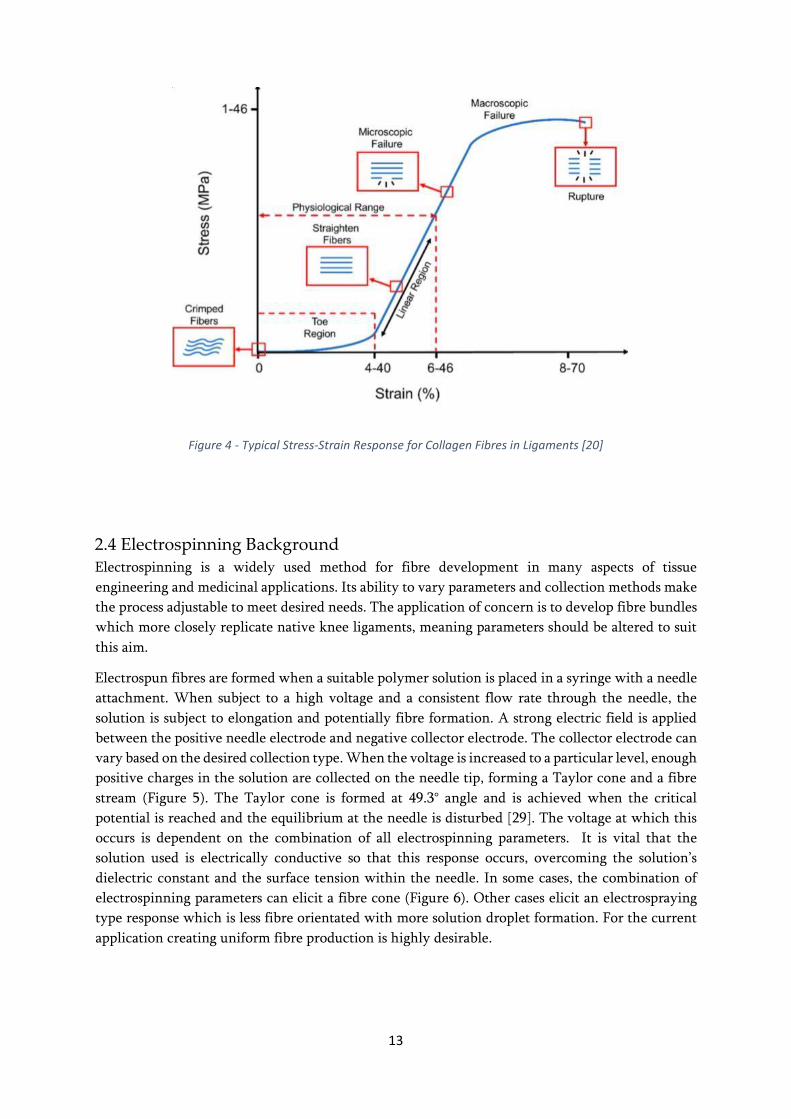
The matrix of the ligament follows a sinusoidal type wave, referred to as ‘crimp’. The crimp pattern
straightens out during low loads of tensile stretching without causing damage to the fibrils. Under
larger loads, the fibrils are elongated, with more fibril elongation as the load increases [19]. This
type of non-linear response can be represented in a force-displacement or stress-strain curve (Figure
4). As all fibrils are recruited with increasing load, the gradual increase in stiffness can also be
interpreted. Beyond the toe region into the linear region is where the elastic modulus of the fibres
can be determined. It will be most desirable for electrospun fibre bundles to exhibit this type of
behaviour and the correct stiffness range when subject to tensile loads.
Image removed due to copyright restriction.
13
Figure 4 - Typical Stress-Strain Response for Collagen Fibres in Ligaments [20]
2.4 Electrospinning Background Electrospinning is a widely used method for fibre development in many aspects of tissue
engineering and medicinal applications. Its ability to vary parameters and collection methods make
the process adjustable to meet desired needs. The application of concern is to develop fibre bundles
which more closely replicate native knee ligaments, meaning parameters should be altered to suit
this aim.
Electrospun fibres are formed when a suitable polymer solution is placed in a syringe with a needle
attachment. When subject to a high voltage and a consistent flow rate through the needle, the
solution is subject to elongation and potentially fibre formation. A strong electric field is applied
between the positive needle electrode and negative collector electrode. The collector electrode can
vary based on the desired collection type. When the voltage is increased to a particular level, enough
positive charges in the solution are collected on the needle tip, forming a Taylor cone and a fibre
stream (Figure 5). The Taylor cone is formed at 49.3° angle and is achieved when the critical
potential is reached and the equilibrium at the needle is disturbed [29]. The voltage at which this
occurs is dependent on the combination of all electrospinning parameters. It is vital that the
solution used is electrically conductive so that this response occurs, overcoming the solution’s
dielectric constant and the surface tension within the needle. In some cases, the combination of
electrospinning parameters can elicit a fibre cone (Figure 6). Other cases elicit an electrospraying
type response which is less fibre orientated with more solution droplet formation. For the current
application creating uniform fibre production is highly desirable.

14
Figure 5 - Solution Impact with Increase in Voltage, Taylor Cone Formation at C [24]
Figure 6 - Typical Electrospinning Setup [25]
The type of collection most desirable for synthetic ligament applications is the use of a rotating
mandrel. By employing a high-speed rotating collector, the fibres can be collected with some stretch
and over a large surface area. This collection method would be most beneficial in replicating the
natural fibre structure of ligaments, allowing for bundling of the fibres after collection. There are
limitations in aligned fibre production since the high electric field in a short distance induced
whipping in the fibre jet, potentially widening the cone before it lands on the collector. It is worth
ensuring the electric field can be controlled by the applied voltage and the distance between the
electrodes. In cases where the distance is too small, the solution may not have sufficient opportunity
to dry and for the solvent to evaporate, leaving wet fibres or solution droplets on the collector.
There are also limitations with knowing what type of fibres are being produced during testing as
they are nanoscale structures. Although the type of jet can be indicative of the fibre production, the
use of a nanoscale imaging device will provide conformation of the fibre size and orientation.
2.5 Parameter Impact on Fibres The characteristics of the fibres that are formed are dependent on the electrospinning parameters
set during the process. The polymer’s concentration and molecular weight in the solution used,
directly impacts the fibre diameter. In cases where all electrospinning parameters are kept constant
Image removed due to copyright restriction.

15
and only concentration in altered, it is expected higher concentrations result in thicker fibre
diameters. Based on the given experimental findings, the higher the molecular weight, the higher
tensile loads the specimen is capable of withstanding. Again, with consistency in all other
parameters, increasing voltage, electrode distance and mandrel rotational speed independently, the
fibre diameters will be decreased [21]. All these factors need to be considered when developing
fibres for this particular application.
Due to the specific microstructure of each knee ligament, it is vital to collect the electrospun fibres
in a way which replicates or closely matches the ligament structure. Ideally, the synthetic samples
should have aligned bundles of fibres which exhibit some crimping. A worthwhile method in order
to achieve this is to use a rotating mandrel as the negative electrode. Fibres can be collected in an
aligned state when the mandrel is rotated at high speeds. Rolling the fibres off of the mandrel is a
suggested method for having both aligned and bundled fibres [20] (Figure 7). Perfecting the
collection method will be pivotal in achieving similarity of the native ligaments on a
microstructural point of view.
The production of electrospun fibres are also subject to variation based on ambient conditions. The
surrounding temperature and humidity of the testing conditions will influence the extent the
solvents will be evaporate in the fibre formation and collection [29]. The temperature also has the
ability to affect the conductivity of the solution. This is due to the weakening or strengthening of
the intramolecular forces, which in turn affects the polarity of the solvent. Once the polarity is
affected, the applied voltage may need to be altered accordingly to still produce a desired response.
Image removed due to copyright restriction.

16
Figure 7 - Method for Aligned Fibre Bundle Collection [27]
2.6 Mechanical Properties A key aspect of developing synthetic knee ligaments is that the mechanical properties are within
the same range of a native ligament. A common ACL replacement procedure is the use of a sectioned
patellar tendon. While the biocompatibility is high if sourced from the patient, the elastic modulus
is found to range between 597 to 843 MPa [30]. This range indicates that the patellar tendon is too
elastic and not stiff enough to be used as a replacement for any of the knee ligaments, highlighting
the importance of producing a replacement with a more desirable elastic modulus.
A series of papers were investigated to determine the stiffness range of the electrospun ligament
should lie in (Table 1). There were many exclusions as comparisons were made to animal models
rather than human. The animal models may be regarded as outliers and give an inaccurate
representation of the stiffness range, and hence were excluded. The majority of studies also put a
focus on the ACL without consideration for the other ligaments.
Table 1 - Stiffness and Elastic Modulus Range of Native ACL
Source Native
Ligament
Specimen
no.
Stiffness
(N/mm)
Elastic
Mod. (MPa)
13 ACL (48-86 yrs) 20 129±39 65.3±24
ACL (16-26 yrs) 6 182±56 111±26
14 ACL (male 2650
yrs)
8 308±89 128±35
ACL (female
17-50 yrs)
9 199±88 99±50
Table 2 - Stiffness Ranges for Native PCL, MCL, LCL
Ligament Stiffness Range (N/mm) Elastic Modulus (MPa)
ACL 129 – 308 65.3 – 128
PCL 64 – 107
MCL 53 – 86
LCL 68 - 84
Table 3 - Stiffness Range Summary of all Knee Ligaments
Source Native
Ligament
Specimen
no.
Stiffness
(N/mm)
22
(L141432)
PCL 1 107
MCL 1 83

17
LCL 1 84
22
(S142395L)
PCL 1 86
MCL 1 53 – 57
LCL 1 68
22
(S142444L)
PCL 1 64
MCL 1 61
LCL 1 75
22
(142444)
PCL 1 64
MCL 1 68
LCL 1 73
Even though a stiffness summary was made based on the four key knee ligaments, the ACL was the
focus in most studies, so the stiffness range was established with the values from ACL findings.
There is difficulty making a direct comparison across all studies as all used different mechanical
tests and procedures. However, all four ligament ranges will be useful when developing electrospun
samples to determine whether the specimen stiffness’s match a particular ligament.
As studies varied based on method and testing, only those which provided a stiffness or elastic
modulus value could be considered. Even with this normalisation, the samples were made up of
different shapes and pore sizes, hence affecting the cross-sectional area of the synthetic ligament.
This of course is a factor that needs to be considered in determining the elastic modulus.
2.7 Research Variations The span of the electrospinning synthetic ligament research is quite broad with a great deal of
variation in the research aims. Although most papers place a specific aim to replicate the ACL in
some way, be it through fibre diameters or mechanical properties, materials used, electrospinning
parameters and methods, all have significant variance.
The properties of the fibres produced have a high dependence on the materials used in the solution.
The polymers, solvents and concentrations used was the first aspect to separate the studies.
Although some experiments have overlaps in the materials used, the parameters overall methods
vary too drastically to make a direct comparison. The key electrospinning parameters are outlined
so that a suggested range for each aspect could be established (Table 4).
As all studies had various aims, the results and outcomes of each are fairly varied. Some place
emphasis on the fibre diameter, while other studies focus on mechanical properties. There were
some papers which have aims surrounding pore size, cell attachments and in vivo testing, which is
beyond the scope of this study. Based on all results, a summary of outcomes has been outlined (Table

18
5), however those that provide information about stiffness or the elastic modulus can be considered
further for experimental guidelines.
The considerations which need to be made when mechanically testing the samples relates to the
porosity, size and shape. While some cases follow a desired porosity percentage, others intentionally
aim to eliminate pores within the samples for more accurate mechanical testing. This is because the
closely packed fibres provide a cross-sectional area not compromised by spaces between the fibres
and therefore more accurate calculations of stress. Some studies laser cut pores to result in a 15%
porosity and a specific pore diameter suitable for cell ingrowth [5, 10, 11]. These cases are tested
post-implantation, where the cells make contributions to the sample’s mechanics. Some studies
employ specific mechanical testing techniques where the samples are subject to some weight which
flattens the overall structure, condensing the fibres [2]. The porosity remains higher than a native
ACL, however more accurate mechanical testing can take place with a more condensed structure.
The previously mentioned differences in testing method means that a caution when testing will
need to be taken for result accuracy. The degree of porosity is likely to vary with the fibre thickness,
the collection method and its rotational speed. Ideally, consistency should be aimed for through
each test, however it is likely that variation in parameters will be required to have consistent fibres.
Table 4 - Electrospinning Experiments with Key Parameters
Polymer Solvent Voltag
e (kV)
Distanc
e (cm)
Flow rate
(mL/h)
Needl
e
Mandrel
RPM
Additional Info.
1 20%
polyurethane
DMF 14 20 18G 620.7
2 10% PCL (80,k mw) and oleic acid sodium
salt 97:3
3 chloroform : 1
methanol
15 10 2.5 18G
flat tip
3000
3 5% P(LLA-CL) 3:1
DCM/DMF
15 15 0.3mL/mi
n
21G
blunt
tip
1000 Additional heating
for crimping
4 13% PLLA
(84,000 mw)
65:35
DCM/DMF
18 20 1.2 2-40mm apart 18G
2900

19
5 10 % PCL
(110,000
Mw)
1,1,1,3,3,3hexafluro2
-propanol
20 2.5 3450 Pores were laser cut
Bathed in EtOH
and collagen
6 20 % PLGA
(153,000 mw)
(60:40) acetone/D MF
21 20 3 18G
flat tip
612.1 Fibres land in water bath,
rotating mandrel
next to it
7 7, 12, 20%
PEUUR (146
kDA mw)
1,1,1,3,3,3hexafluro2
-propanol
15 15 3 22G 9.5m/s
8 15% poly(Llactic-
co-e- caprolactone)
( PLCL (LA/CL
70/30))
(90/10) chloroform/ DMF)
6-9 15 2 19G 1500 Scaffolds were
knitted after
electrospinning
9 20 – 35% poly(L-
lactideco-acryloyl
carbonate) (P(LLA-AC))
3:1 dichlorome thane/DMF
15 15 1.8 21G 1000 Crimping in 37 degree C
phosphatebuffere
d saline
1
0
10%
UHMWPCL
(500kDa)
1,1,1,3,3,3hexafluro2
-propanol
25 0.7 1725 Laser cut stacked mats – bathed in
70% EtOH
10% PCL
(80kDa)
1,1,1,3,3,3hexafluro2
-propanol
20 2.5 3450
1
1
10% PCL in chloroform
(140k g/mol)
1,1,1,3,3,3hexafluro2
-propanol
20 2.5 3450
1
2
5,11, 16%
PLGA
1,1,1,3,3,3hexafluro2
-propanol
15 15, 12 5 22G
Teflon
tip
Stationary
,
580,1010
1450
1
5
18% PLGA 70/30
(THF:DMF)
20 15 1 0.8 mm
diam.
3000
Table 5 - Electrospinning Experiments Result Summary
Source Fibre Diameter Specimen
size
Pore
size
Pore area
%
Young’s
Modulus
(MPa)
Ultimate
Strength
(MPa)
Yield
Stress
Stiffness
(N/mm)
1 657±183 nm 10 X 40 X 1
mm^3
0.0032
– 366.7μm
(diamet
ers)
82.72 3.55 3.52

20
2 474±57μm 3.17 mm W
4cm L
5μm 154 ± 28
3 0.88 ± 0.002
µm
0.349 193±44
kPa
4 550-600 µmbundle
0.59±0.14 µm
100mm L
6.5mm
diameter
156.2±36
7
15.8±2.8
MPa
5 1.5mm X
35mm X 900μm
(stacked
sheets)
150μm
(laser
cut)
15% 1.95±0.3
5
6 2.15 ± 0.55 µm
(parallel fib.)
32 × 5 mm2
(rectangle)
775 ± 35
7 (7) 0.50±
0.11mm
(12) 1.08±
0.22mm
(20) 2.08±
0.57mm
8 2.6 ± 0.3 μm
(aligned)
202±12 46±4
9 (12% AC) 0.85 ±
0.10 μm
26±1.4
10 1.5mm X
35mm X 150
μm
150 μm
Laser
cut
15%
11 1.5mm X
35mm X 150
μm
15% 6.2±3.9
12 (Stat.)
0.014±0.07 μm 0.076±0.36 μm
3.6±0.6 μm
15 900 nm 129.07±2
0.22
Those studies which provided a stiffness or elastic modulus within or close to the range previously
found for the native ligaments where further summarised with comparison to the electrospinning
parameters used (Table 6). As desirable outcomes were achieved in these cases, this gives a good
indication on the test parameters and materials which can be used to produce the synthetic
electrospun ligaments.

21
Table 6 - Top Selection Electrospinning Experiments
Polymer Solvent Voltage
(kV)
Dist.
(cm)
Electric field
(kV/cm)
Flow rate
(mL/h)
Needle Rpm E
(MPa)
2 10% PCL
(80,000mw)
and oleic acid
sodium salt
97:3
3 chloroform : 1 methanol
15 10 1.5 2.5 18-G flat tip 3000 154 ±
28
4 13% PLLA
(84,000 mw)
65:35
DCM/DMF
18 20 0.9 1.2 2 syringes
(40mm apart) 18G
2900 156.2
±36.7
8 15% poly(Llactic-co-
e- caprolactone)(
PLCL (LA/CL
70/30))
(90/10) chloroform/
DMF
6-9 15 0.4-0.6 2 19G 1500 202±1
2
15 18% PLGA 70/30
(THF:DMF)
20 15 1.33 1 18G 3000 129.0 7±20.
22
2.8 Overview of Proposed Study
2.8.1 Aim
To develop an electrospun ligament replacement which closely mimics the elastic modulus and
microarchitecture of a native human ligament. Achieving this would mean development towards a
graft which is most similarly matched to the original ligament without compromise to the overall
mechanics of the knee.

22
2.8.2 Objectives
The aim will be achieved through explorative testing of polycaprolactone (PCL) in various
combinations of dimethylformamide (DMF) and chloroform. Collection method will also be tested
so that efficient fibre collection can take place while achieving the desired alignment. The
microarchitecture of the samples will be viewed on SEM imaging techniques, while the elastic
modulus will be determined through tensile testing.
Many studies aim to create a replacement using electrospinning methods, but then further the study
with cell seeding and in vivo testing prior to perfecting these two key aspects. There was no study
found to simply develop a synthetic ligament, not only limited to the ACL, and provide information
on both its microarchitecture and its stiffness. The explorative nature of this study aims to do so,
potentially progressing the development of synthetic knee ligaments.
2.8.3 Justifications of Decisions
Various combinations of polymers and solvents can be used in electrospinning, yet the materials
should reflect the desired outcome. An overview of polymers with potential applications were
assessed in order to give conformation to decisions made [20]. Although there would be value in
testing a number of materials, limitations are placed on the polymer and solvent option due to both
budget and timeframe limitations. There was attraction toward the use of polycaprolactone (PCL)
due to is proven biocompatibility as its Food and Drug Administration approval in some human
body applications [31]. Also, PCL with a molecular weight of 80,000 Mn has proven to elicit
desirable results based on the studies outlined previously. The use of PCL was also attractive based
on the price of the quantity required for multiple tests. Based on the properties of solvents,
chloroform was selected for its high PCL solubility, while dimethylformamide (DMF) was selected
due to its high dielectric constant and electrical conductivity. With focus on the use of PCL in
combination with various concentrations of chloroform and DMF, this study will aim for the best
results with these materials and within the electrospinning machine specifications.
2.8.4 Overview of Experimental Method
Given the concentration ranges of the polymers in Table 6, the PCL will be tested in concentrations
of 10, 13, 15, 18 and 21% w/v. As the PCL tested has a relatively high molecular weight, it will be
important to ensure the polymer is completely capable of dissolving in the solvents. There is more
difficulty in dissolving PCL in DMF compared to chloroform, however DMF does prove to have
benefits in fibre production, as seen in three of the four top experimental picks (Table 6). For this
reason, it will be valuable to establish various solvent ratios to determine which solutions produce
better performing fibres. For each concentration, the solvent ratios will be 100:0, 25:75 and 50:50
in favour of both DMF and chloroform, producing 5 solvent combinations for each polymer
concentration.
Naturally, with variation in concentration and solvent ratios, the viscosity of the solutions will vary.
This may impact the needle type that should be used and the flow rate of the solution coming
through it. The range established from the studies is from 1 to 2.5 mL/h with 19G or 18G needles.
Although a reliable guide, it will be important to experimentally establish what the ideal fibre

23
production case is. If the development of fibres is not consistent within these ranges, further testing
will need to be done to do so.
The electric field can be adjusted by the voltage applied but is most likely limited by the distance
between the electrodes. If the position of the rotating mandrel cannot be adjusted, the applied
voltage will determine the strength of the electric field during testing. With the voltages ranging
from 6 to 20 kV, the potential difference is expected to be in this range but will be more reflected
on the amount which produces a consistent fibre stream. This will need to be experimentally tested
as some applied voltages exhibit consistent fibre streams for a short period of time before the voltage
dries the solution at the tip of the needle, inhibiting solution flow. To avoid this, it is important to
determine a voltage which is capable of producing consistent results for a longer duration, allowing
a large amount of fibre collection with each test.
The rotational speed of the mandrel in the studies vary from 1500 to 3000 rpm. It has been
discovered that higher speeds produce smaller fibre diameters which may impact the elastic
modulus of the overall sample, but the combination of the other parameters will also have an
impact. There is benefit in varying the rotational speeds in attempt to create some crimping within
the fibre bundles but the importance lies in having aligned fibres in the collection method.
The assessment of the electrospun ligaments will be determined by scanning electron microscope
(SEM) imaging. These images will be vital in determining whether the fibres have been collected
in an aligned manor and if the microarchitecture matches a native ligament. Image processing
techniques will also be employed to calculate the average fibre diameter of the samples. Although
not a key objective, there is value in determining how the parameter combinations affect the fibre
diameters.
Tensile testing where force and displacement are measured is important to determine the stiffness
of the samples and ensure it lies within the native ligament range established previously. This is
another key aspect which will determine if the samples are sufficient for use as a synthetic knee
ligament.
3. MethodologyThe method established was done so for the consistency of ligament sample formation. Although
sections of the procedure were subject to systematic error, the procedure was aimed to lie within
the testing bounds. Experiments were conducted on the NEU-Pro Electrospinning Unit
(Manufactured in China).
3.1 Solution Preparation Chemical materials were purchased from Sigma-Aldrich, where the PCL had a molecular weight of
80,000 Mn. Solutions were made with various amounts of PCL and solvent combinations to uphold
with the previously outlined concentrations and ratios. The concentrations were based on all
samples being made up of 10mL of solvent, according to which ratio was being used (Table 7).
Table 7 - Solvent Ratios

24
Solvent ratio type Chloroform (mL) DMF (mL)
1 10 0
2 7.5 2.5
3 5 5
4 2.5 7.5
5 0 10
All solutions required a relatively long dissolving time so were placed on a magnetic mixer with a
small magnet inside the solution. Chloroform-heavy solutions dissolved at a quicker rate than those
with predominantly DMF as the solvent. Despite the solvent ratio, dissolving time was
approximately 24 hours. Even after 48 hours and more, the PCL did not dissolve in the 100% or
75% DMF solutions, proving early on that this particular molecular weight PCL is too high for the
DMF to dissolve and could not be tested.
Although the other three solvent combinations were completely dissolving the PCL, not all were
worth testing. The 100% chloroform solution proved to be difficult to test in the electrospinning
device, with inconsistent parameters and unpredictable fibre jet making it difficult to produce
consistent results. Due to these complications, only type two and three solvent ratios were used in
further testing.
3.2 Electrospinning Procedure The solution was placed into the 10mL syringe which was connected to one end of the plastic
tubing. On the other end of the tubing, the 18G flat tip needle was connected. The 18G needle was
trimmed and filed down in order to have a flat tip. This was necessary in testing as charges would
accumulate on the tip of the needle when it was subject to high voltage. This charge accumulation
may affect the development of the Taylor cone when it comes to fibre production as well as the
trajectory of the fibre jet. The needle distance from the collector was kept constant for all tests at
15cm.
Between each test, the tube was flushed with chloroform to prevent and contamination between
the solutions. For the electrospinning testing, the needle was fed through the device and placed in
the left needle holder, while the syringe on the other end was placed into the flow rate pump (Figure
8). Prior to setting the flow rate, the solution was purged in order to push the solution to the tip of
the needle. Some cases required purging until the solution was consistent and free of air bubbles in
the tubing. Once the solution was set up, it was placed in the syringe pump where the flow rate
could be set.
25
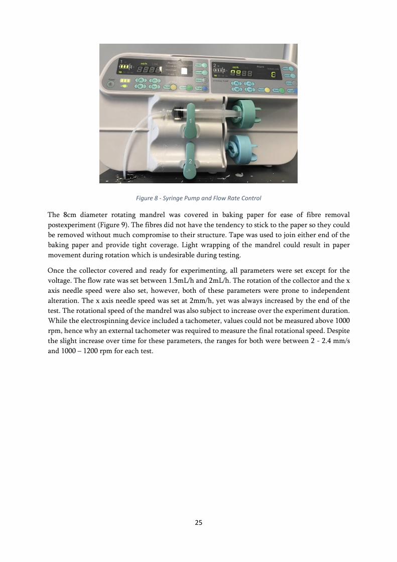
Figure 8 - Syringe Pump and Flow Rate Control
The 8cm diameter rotating mandrel was covered in baking paper for ease of fibre removal
postexperiment (Figure 9). The fibres did not have the tendency to stick to the paper so they could
be removed without much compromise to their structure. Tape was used to join either end of the
baking paper and provide tight coverage. Light wrapping of the mandrel could result in paper
movement during rotation which is undesirable during testing.
Once the collector covered and ready for experimenting, all parameters were set except for the
voltage. The flow rate was set between 1.5mL/h and 2mL/h. The rotation of the collector and the x
axis needle speed were also set, however, both of these parameters were prone to independent
alteration. The x axis needle speed was set at 2mm/h, yet was always increased by the end of the
test. The rotational speed of the mandrel was also subject to increase over the experiment duration.
While the electrospinning device included a tachometer, values could not be measured above 1000
rpm, hence why an external tachometer was required to measure the final rotational speed. Despite
the slight increase over time for these parameters, the ranges for both were between 2 - 2.4 mm/s
and 1000 – 1200 rpm for each test.

26
Figure 9 - Rotating Mandrel Collector Covered in Baking Paper
Figure 10 – NEU-Pro Electrospinning Unit

27
The flow rate parameter was turned on and once solution consistency through the tube was
achieved, the voltage was increased until a continuous fibre jet was created. As fibre streams and
jets were fine and difficult to see, caution was taken with parameter adjustments. Smaller
concentration solutions would produce shorter streams and larger, more visible fibre jets (Figure
11), while solutions with larger concentrations generally produced longer streams but much finer
and shorter fibre jets (Figure 12). The best fibre jet results were seen at approximately 20kV,
however adjustment of voltage was made until a continuous fibre jet was formed. For instances
where the fibre jet was inconsistent or splattering, for the purpose of consistency amongst other
parameters, the voltage was the only parameter changed to produce a more desirable fibre jet. If
splattering of the jet or solution dripping was occurring, to produce stability the voltage was
increased. In cases where the fibre jet was becoming small or the Taylor cone was appearing to dry
out, the applied voltage was decreased.
Figure 11 - A) Short Fibre Stream B) Long Fibre Jet

28
Figure 12 - A) Long Fibre Stream B) Shorter, Finer Fibre Jet
Each test was given a two-hour time period for fibre collection. Some test has a shorter duration of
if the solution in the syringe ran out before the two-hour time had been reached. Upon completion,
the parameters would all be safely stopped, with consideration towards not having remaining
solution droplets onto the collected fibres. The fibre sheet was removed by horizontally slicing the
baking paper with a scalpel while on the mandrel, allowing the sheet to be spread out flat (Figure
13). Once the baking paper was removed, the section of the sheet with tape was also sliced out. This
section was saved in some samples for later SEM imaging. The remainder of the sheet was halved
so that from one test, two ligament sample could be made.

29
Figure 13 - Removed Baking Paper with Fibre Sheet
The ligament samples were created by rolling up the fibres in the same, longitudinal direction of
collection. This was done by placing another sheet of baking paper on top on the edge of the sheet.
Since fibre amounts are scarcer along the edges, to start the rolling up of the fibres they need to be
handled delicately. Once the edge was lifted, the remainder of the fibre sheet could be consistently
and carefully rolled up (Figure 14).
Figure 14 - Rolled-up Fibre Sheet into Ligament Sample
The weight and length of each sample was measured and recorded so that data normalisation could
be done for the mechanical tests. The length was considered from each edge of the fibre sheet. If

30
the ends were thin due to uneven rolling, the length was considered from the visible edge of the
fibre sheet on either end. Callipers were also used to carefully measure the diameter of the sample,
taking care not to compress the fibres. This measurement was taken in a middle portion of the
bundle, where the most consistent thickness was found to be. The diameter was halved, using the
radius to find the cross-sectional area of the circular fibre bundle. There was some difficulty in
taking this measurement as not all fibre bundles were tightly wrapped, introducing possible error
in the diameter measurements. This however, would be accounted for in the data normalization.
The electrospinning tests were conducted in three different rounds. The first round covered a range
of polymer concentrations in order to determine which solutions are most successful to electrospin
with as well as to gain understanding of the material properties of each. Following the first round,
the second and third lot of electrospinning tests were done with focus on the more successful
solutions. The success of the solution is based on its cooperation in the electrospinning environment
and the mechanical information it provides.
3.3 Mechanical Testing Mechanical testing and data analysis was followed by each significant electrospinning round.
Evaluation of the sample’s material properties would be achieved through tensile testing, using the

31
Test Resources Machine with clamp attachments (Figure 15). Tests were conducted with a 5 kN
load cell to conduct a position based tensile test at 30% strain rate for each sample. This was decided
as 33% per second strain rate is approximately the strain experienced on the knee ligaments during
walking [4]. Each end of the sample was clamped into the device from which the tests would begin
from. The rate of strain was dependent on the starting distance between the clamps, which was
slightly different with each run. Vertical alignment was maintained by clamp both ends with the
guidance of a metal ruler.
Figure 15 - Test Resources Device for Tensile Testing
Ideally the breaking of the ligament would occur in the middle of the testing region, however due
to the stress concentration at the clamps, occasionally the ligament samples would break directly at
the clamped location (Figure 16). The inside of the clamps were entirely made up of knurling grip,
which with its sharp nature, the tight clamping had a tendency to potentially produce cuts in the
samples. The data resulting from these types of test can still indicate the linear region of material
but cannot account for the ultimate load the sample can withstand. This is particularly evident in
cases where data appears to enter a second linear phase, suggesting some yielding has occurred
sooner than anticipated.

32
a) b)
c) d)
Figure 16 - a) Increased strain prior to b) Incremental breaking c) Increased strain prior to d) Clamp breaking
To avoid premature yielding or any other impacts from the knurling grip, an addition testing
method was employed for later third round tests. The samples were folded over on either and looped
once through metal rings fashioned out of thin wire. The ends were then secured with electrical
tape and securely tightened with a clinch knot (Figure 17). The distance measured for each of the
tests was done from knot to knot rather than from clamp edge to clamp edge while the remaining
test methods were kept consistent. This information is vital for the determination of the strain rate
the test would operate at and later required for the calculations for overall strain of the sample. The
metal ring was then placed in the clamps, avoiding any force on the samples. The tensile test would
then be conducted with data recorded for interpretation of the mechanical behaviour.

33
a) b)
Figure 17 – a) Looped end sample prior to testing b) Looped end samples during testing
3.4 Normalising Data As each sample had a different length, weight and cross-sectional area, it was important to use this
information to normalize the mechanical testing data. Although the majority of tests were
conducted with a 1.5mL/h flow rate and a two-hour duration, the fibre jets created for each run
varied, meaning the types of fibres being formed were dependent on the other parameters. Due to
these impacts, fibre sheet thickness varied for each run, which also made an impact on the type of
rolling each test was capable of. Thin fibre sheets were more subject to scrunching or folding,
making it difficult to tightly roll the sheet. In these instances, the cross-sectional area would appear
slightly larger than it should be, impacting the comparison for stress calculations. The stress formula
accounts for a solid object, which these samples are not. However, dividing apparent stressed by the
material volume fraction accounts for the lack of solid material in the samples (Equation 1).
𝑤 (𝑘𝑔)
𝑀𝑎𝑡𝑒𝑟𝑖𝑎𝑙 𝑉𝑜𝑙𝑢𝑚𝑒 𝐹𝑟𝑎𝑐𝑡𝑖𝑜𝑛 (𝑣) = 𝐿 (𝑚) × 𝐴(𝑚2) × 𝜌(𝑘𝑔𝑚−3) (1)
The data recorded from the Test Resources machine was the relative force and stroke, both which
were used to calculate the respective stress and strain for each sample. The data was recorded just
prior to testing and the force and stroke values were negative or close to zero during this time. The

34
data used in the plots would be from when the stroke value was greater than zero, indicating the
test had begun. The corresponding force value in each case was always slightly above zero, due to
the weight of the clamps. The force was not reduced to a starting point of zero since the values were
so minute and there would be no impact to the slope of the linear region. The calculated
crosssectional area and the initial distance between the clamps were used in the stress and strain
equations (Equation 2, 3). The stress was normalized by dividing through by the material volume
fraction. The stress-strain curves were graphed using MATLAB, where the strain was not graphed
as a percentage in order to calculate the Young’s modulus from the graph (Equation 4). Since each
case was very specific in terms of breaking and data noise, the linear region’s varied and needed to
be judged accordingly. The noisy graphs were smoothed in MATLAB, clearing the visual aspect of
the graph. The slope was found between two points which were evidently linear in the smooth
graphs, which were proved with the R2, however noisier graphs required multiple measurements
to find an appropriate average.
𝐹 (𝑁𝑒𝑤𝑡𝑜𝑛𝑠)
𝑆𝑡𝑟𝑒𝑠𝑠 (𝜎) = 𝐴 (𝑚2) 𝑣
(2)
∆𝑙
𝑆𝑡𝑟𝑎𝑖𝑛 (𝜀) = (3)
𝑙0
′𝑠 𝑀𝑜𝑑𝑢𝑙𝑢𝑠 (𝐸) = 𝜎 (𝑃𝑎𝑠𝑐𝑎𝑙𝑠) (4)
𝑌𝑜𝑢𝑛𝑔 𝜀 (𝑢𝑛𝑖𝑡𝑙𝑒𝑠𝑠)
3.5 SEM Imaging Method A small section of the fibre sheet was saved from each test in order to analyse the fibres on a
microscale with the FEI Inspect F50 model scanning electron microscope. Since the drum was
covered in baking paper, the join of the paper was connected using tape. The fibres between the
tape were left flat as they landed. Each sample was prepared on a small metal stage and pressed on
a secured to double-sided tape.
The samples then underwent sputter coating which covered the surface of the fibres with a thin
platinum film (

35
Figure 18). Since imaging takes place though the reflection of an electron beam the samples were
layered with additional platinum coating to make the surface of the fibres more conductive. The
fibres are conductive enough to be imaged without the coating, however, the additional layer makes
the fibres less subject to movement due to the electron beam, since the fibres are not tightly secured.
The samples were placed in the device mount and vacuumed sealed for five minutes. After the
coating, the fibres appear to have a slightly grey tinge, none of which negatively impacts the
imaging process.
Figure 18 - Samples post sputter coating
Upon sputter coating, the metal fibre holders were placed onto a dedicated imaging stage within
the SEM vacuum (Figure 19). This section could be opened for samples to be placed, while the
filament and anode which drive the electron beam remain in a sealed off vacuum which cannot be
accessed. Once placed, this section was closed off and vented in order to match the vacuum of the
beam section. The closed section can still be viewed via and internal camera and imaging software
to the linked computer. This enables the controlled imaging of each sample while still being to
identify each sample.
The saved images were imported into Fiji, where the scale was set according to the magnification
of each image. The known distance in the images were used to find a ratio to the number of pixels
in that given length. Setting the scale enabled for measuring of the fibre diameters seen on the
surface. It was important not to consider the fibres which were placed under other fibres or in the
distance of the image as there was no method to determine the depth at which they were.

36
a) b)
Figure 19 - a) SEM with open chamber b) Samples placed on chamber stage prior to imaging
4. Results4.1 Electrospinning Outcomes The parameters were aimed to be as consistent as possible, however, some variation was experienced
with each test. Each electrospinning round divided and the parameters recorded so that variations
or outliers could be easily identified (Table 8, Table 9, Table 10). The samples were paired off since
each electrospinning run would produce a fibre sheet long enough for two samples, hence the
sharing pf parameers. Even with difficulty in controlling the rotational speed, the values were
measured in order to correlate to fibre diameter upon imaging. The values for applied voltage had
the greatest variation, however, adjustment was required to produce worthwhile fibres. The
inconsistencies may be due to ambient conditions or other external factors.
Table 8 - Round One Electrospinning Test Parameters
Ligament
sample
no.
Conc. Of
PCL (%)
Solvent ratio
(DMF:CHCl3)
Flow rate
(mL/h)
Voltage (kV) Final Rpm Run
time
L1/L2 10 25:75 1.5 20-22 1000+ 2h
L3/L4 10 50:50 1.5 20.04 1000+ 2h
L5/L6 15 25:75 1.5 20.02 1000+ 94 min
L7/L8 15 50: 50 1.5 25 1000+ 2h
L9/L10 18 25:75 1.5 20.09 1098 2h
L11/L12 18 50:50 1.5 20.05-22 1108 2h
L13/L14 21 25:75 2 20.08 1538 <2h

37
L15/L16 21 50:50 1.5 20.07 – 22.05 950 -1257 2h
Table 9 - Round Two Electrospinning Test Parameters
Ligament
sample no.
Conc.
Of PCL
(%)
Solvent ratio
(DMF:CHCl3)
X axis needle speed
(mm/s)
Flow Rate
(mL/h)
Voltage
(kV)
Final
Rpm
Run
time
L17/L18 10 25:75 2.1-2.4 1.5 20.05 1233 2h
L19/L20 10 25:75 2.1-2.4 1.5 20.02 1080 2h
L21/L22 10 50:50 2-2.4 1.5 20.03 1080 2h
L23/L24 10 25:75 2.1-2.4 1.5 20.08-
23.03
1032 2h
L25/L26 10 50:50 2-2.3 1.5 25.11-
30.12
1088 2h
L27/28 10 50:50 2.2-2.3 1.5 25.49 1047 2h
L29/30 10 50:50 2.3-2.4 1.5 20.02 1050 2h
Table 10 - Round Three Electrospinning Test Parameters
Ligament
sample no.
Conc.
Of PCL
(%)
Solvent
ratio
X axis needle speed
(mm/s)
Flow Rate
(mL/h)
Voltage
(kV)
Final
Rpm
Run
time
L31/L32 13 25:75 2-2.3 1.5 26.3-35.01 1102 2h
L33/L34 13 50:50 2-2.3 1.5 25.05 1102 2h
L35/L36 13 50:50 2.3-2.4 1.5 20.06 1105 2h
L37/L38 13 25:75 2.3-2.4 1.5 20.02-
23.03
1107 2h
4.2 Material Properties of Ligament Samples The stress-strain curves were used to determine the Elastic Modulus (Young’s Modulus (E)) for each
of the ligament samples. This value was determined by the slope in what appeared to be the linear
region for each case. Some linear regions were prematurely shortened due to clamp stresses,
however the slopes were determined across the entire span of each linear region. The strain was
not represented in percentage in the graphs so that the values could be used in elastic modulus
calculations. The type of break or whether the sample broke at all can be seen in the stress-strain
graphs. The evidence in premature clamp breaking due to the knurling grip can be seen in cases
such as sample L6 since the linear region is relatively short and a second linear region is experienced,
possibly where the remainder of the fibres were elongated prior to the complete break load (Figure
20). Despite premature yielding in some cases, there were samples which still experienced
incremental breaks, such as sample L12 (Figure 21). In the direct knurling clamp cases, no toe region

38
is seen, which suggests the fibres are already straightened, or a portion of them were damaged and
cannot be incrementally recruited.
Figure 20 - Stress-strain graph of sample L6
There were also clamped method cases which did not break, this was a common occurrence for the
ligament samples made with concentrations of 18 or 21% w/v. These samples also prove to have a
very distinct elastic region and yielding point. An ultimate load cannot be determined since failure
did not occur, as evident in sample L9 (Figure 22). For those ligaments that did not break, the real
time data showed that at the constant strain the was held at the end of the test, the force experienced
was slightly lowered overtime, also relates to the stress being reduced with time. This is an
indication that the material exhibits stress relaxation when subject to a constant strain, proving its
viscoelastic properties.

39
Figure 21 - Stress-strain curve for sample L12
Figure 22 - Stress-strain curve for sample L9
An improvement was seen in the graphs when the looped end method was employed over the
clamping test method. The fibres were less subject to early breakage at the clamps, which enabled
a less interrupted linear region in most cases. While some ligament samples broke in the middle and
not at the clamping site, others experienced abnormal breaks where the outer layer of fibres was
pulled away from the middle layers. This is most likely due to too much tightening of the string at
the sample’s end, slicing through the outer layer of fibres. There was however, more opportunity
for a toe region to be seen in this method. Despite not all tests being in tension prior to commencing,
there is evidence of incremental fibre recruitment once forces are positive in the recorded data.
This type of behaviour is shown in a cases such as L32 and L34, (Figure 23, Figure 24). It is difficult
to declare whether this is due to some crimping experienced in the fibres or whether the
multidirectional orientation and initial resistance to strain are causing the toe region reaction. There
is some evidence in sample L34, that premature yielding is occurring, with uncertainty to if its
dependent on the tightness of the string. However, the overall result of the graphs in the thirdround
testing had a smaller occurrence of premature yielding.

40
Figure 23 - Stress-strain curve of sample L32

41
Figure 24 - Stress-strain curve of sample L34
The first round of electrospinning was done to compare the concentration of the PCL in the solution
to Young’s modulus. The most closely matched outcome to the native ligament elastic modulus
range would later be reproduced in order to determine the repeatability of the sample development
and testing. The measurements, volume fraction and elastic modulus is for each sample in the first
round of testing is outline for comparison (Table 11).
It was expected that there would be a linear relationship between the polymer concentration and
the elastic modulus, where the modulus would increase with an increase of PCL in the solution.
However, for these testing conditions it is seen that there is the greatest variation across the elastic
moduli experienced for 15% w/v solutions (Figure 25). The large range seen for the 15% solutions
suggests a potential source of error. For samples L5 and L6, test time was slightly below two hours
due to solution limitations. The fibre sheets are likely thinner than in other tests, explaining the
difficulty in rolling them smoothly. Difficulty in rolling may translate into inaccurate crosssectional
area measurements, which as a result impacts the stress calculations. Although a potential source of
error, there is still and inconsistency in trends for higher concentrations. The lack of trend is
indicative of other electrospinning parameters possibly interfering with fibre production and as a
result, the samples material properties.
Although the 10% concentration samples were slightly below the native ligament range, their least
drastic and fairly consistent modulus range made them attractive for secondary testing. Other
concentrations proved to have moduli within the range of native ligaments, but were too
inconsistent to determine which would be best for secondary testing.
Table 11 - Round One Ligament Sample Measurements and Properties

42
Ligament
Sample
No.
Conc.
of PCL
(%)
Weight
(mg)
Length
(mm)
Diameter
(mm)
Crosssectional Area
(mm2)
Material
Volume
Fraction
Elastic
Modulus
(MPa)
L1 10 141.2 105 2.64 5.47 0.215 45.35
L2 10 146.8 104 2.32 4.23 0.292 40.36
L3 10 144 97 2.71 5.77 0.225 31.72
L4 10 146.1 96 2.35 4.34 0.307 40.36
L5 15 166.5 107 3.41 9.13 0.149 207.27
L6 15 162.8 100 2.81 6.20 0.229 243.07
L8 15 217.3 105 3.25 8.29 0.218 115.18
L9 18 262.8 110 4.04 12.82 0.163 123.26
L10 18 234.6 115 3.73 10.93 0.179 129.77
L11 18 256.7 105 3.34 8.76 0.244 179.62
L12 18 241.8 104 3.63 10.35 0.196 179.59
L13 21 406.3 106 6.11 29.321 0.114 157.86
L14 21 320.9 107 4.75 17.7205 0.148 148.99
L16 21 210.9 101 3.29 8.5012 0.215 114.12
Figure 25 - Relationship between PCL concentration in solutions and elastic modulus
The formation of a second round of electrospinning tests was conducted to produce a larger sample
size of the 10% polymer ligaments. The same Young’s calculation method was employed as
previously, using sample measurements, and volume fraction to determine the elastic modulus
(Table 12). The initial clamping test method was kept consistent for all tensile tests, except sample
L26. This sample was tested with the looped end method to inspect the differences in testing
method. It experienced a break at the clinch knot, however the stress strain curve proved otherwise,
with a longer linear region and a toe region (Figure 26).

43
The elastic modulus range was kept fairly consistent, with some values exceeding the previously
found range (31 – 45 MPa). Even with increase in the modulus in some samples, the overall material
property of the 10% solutions was not meeting that of a real ACL. Since only the lower range of the
native ACL was being met in these samples, and the 15% solutions exceeded the desirable elastic
modulus, it was decided third round testing would take place on 13% w/v PCL solutions.
Table 12 - Round Two Ligament Sample Measurements and Properties
Ligament Sample
No. (10% PCL)
Weight
(mg)
Length
(mm)
Diameter
(mm)
Cross-
Sectional
Area
(mm2)
Volume
Fraction
Elastic
Modulus
(MPa)
L17 156.5 108 2.68 5.641 0.224 51.94
L18 156.4 104 2.43 4.6377 0.283 44.53
L19 161.1 104 2.51 4.9481 0.274 63.55
L20 155.5 100 2.44 4.6759 0.290 58.08
L21 151.8 105 2.37 4.4115 0.286 35.15
L22 146.6 100 2.23 3.9057 0.328 45.80
L23 155.9 105 2.41 4.5617 0.284 54.50
L24 162.7 104 2.54 5.0671 0.269 56.59
L25 140.8 104 2.3 4.1548 0.285 31.57
L26 134.9 96 2.1 3.4636 0.354 54.64
L27 144.3 102 2.32 4.2273 0.292 33.74
L28 141.9 99 2.41 4.5617 0.274 38.88
L29 139.6 101 2.4 4.5239 0.267 53.65
L30 141.4 96 2.28 4.0828 0.315 48.78
Figure 26 - Stress-strain curve for sample L26

44
The third round of electrospinning was conducted with all 13% PCL solutions in the same solvent
ratios used for previous tests. Measurements of samples was consistent to previous methods,
summarising the values Table 13). The mechanical testing method was changed from the clamping
set up to the looped ligament end method for all round three samples. This method avoided
premature breaks in most cases and allowed for the incremental recruitment of fibres, showing a
toe region in 50% of the stress-strain graphs. The complete graph summary for round one, two and
three of testing can be seen respectively in Appendix A, B and C.
Table 13 - Round Three Ligament Samples Measurements and Properties
Ligament Sample
No. (13% PCL)
Weight
(mg)
Length
(mm)
Diameter
(mm)
Cross-
Sectional
Area
(mm2)
Volume
Fraction
Elastic
Modulus
(MPa)
L31 176.4 102 3.15 7.79 0.194 92.16
L32 180.9 106 2.98 6.97 0.214 72.49
L33 186.4 104 2.62 5.39 0.290 86.68
L34 199.8 108 2.86 6.42 0.252 106.26
L35 178.5 106 2.61 5.35 0.275 73.73
L36 174.0 106 2.51 4.95 0.289 78.99
L37 191.0 107 3.03 7.21 0.216 69.58
L38 178.9 104 2.80 6.16 0.244 81.86
Based on the summary tables for each electrospinning round, the elastic modulus results most
consistent with native ACL is exhibited by the 13% PCL solutions (Table 13). Despite the variation
across the samples, the values are all within the desired range (65 – 128 MPa) and prove to have a
similar elasticity of real human knee ligaments.
As not all samples broke within the middle segment of the sample, and some samples did not break
within the testing limits, the ultimate load was difficult to obtain. The ligament samples also have
a significantly smaller cross-sectional area than native ligaments, so a direct comparison of ultimate
load cannot be made. The cross-sectional area of the ligaments can be scaled against a native
ligament measurement, determining the factor by which force would be increased. An average
measurement of the ACL cross-sectional area (46.9 mm2) was used to scale against the sample
crosssectional area [42]. Sample L33 was selected due to the nature of its incremental break, where
it experiences a peak load of 41.67 N (Figure 27).
The ACL cross-sectional area was found to be larger than sample L33 by a factor of 8.7. The Young’s
modulus calculation can be rearranged to find an approximation of the force L33 would experience
if it had the cross-sectional area of a native ACL [43]. Due to the nature of the synthetic ligament,
the volume fraction was also included in this calculation, where it is assumed the native ACL has a
volume fraction of one.

45
8.7𝐴𝐸∆𝑙
𝐹′ = 𝑣𝑙0 (5)
𝐹 𝐴𝐸∆𝑙 𝑣𝑙0
8.7𝐴𝐸∆𝑙 𝐹′ 0.29𝑙0
= 𝐴𝐸∆𝑙
𝐹 𝑣𝑙0
𝐹′
= 30
𝐹
The ultimate load experienced by L33 would be increased by a factor of 30 in the case it was the
size of a native ACL, which equates to an ultimate force of 1250 N. Despite not matching the failure
load of a native ACL, which is approximately 2160 N [39], in the case it was developed in to a larger
scale, the synthetic ligament would experience a much larger failure force than what is being
experienced currently. This scaled value is an approximation for one of the samples which
experienced an ideal break, suggesting other samples may have been able to withstand an even
larger load. Exact conclusions cannot be made from this calculation; however, the approximate load
value provides an outline of what would be expected of a synthetic sample had it been manufactured
to the size of a real ACL.
Figure 27 - Stress-strain curve for sample L33
4.3 Fibre Morphology SEM imaging was taken with various magnifications, with adjustments made to produce the best
possible focus in the image. Zoomed out images were taken to get an overall view of the fibre sheet
(Figure 28). Small scale droplets were seen on all imaged samples. Although undesirable, the overall
structure is fibre dependent so it is unlikely that the droplets can make a detrimental impact. A
closer magnification image was taken of each sample in order to assess the fibres and make diameter

46
measurements free of droplets (Figure 29). Suitable images were used in the image processing
program, Fiji, which used the microscope scale and program plugins to find fibre diameters and pore
size.
a) b)
Figure 28 - a) Sample L19/L20 at 2000x magnification b) Sample L29/30 at 1000x magnification
The images are very small portions of the entire fibre sheet, but there appears to be some type of
crosslinking and intertwining of fibres. It is difficult to determine whether this is due to high speed
fibre whipping in the jet or if tis from the nature of PCL as a polymer. Despite the cause, it is
preferred that there is small amounts of this occurring. In the case that there was a great deal of
crosslinking, the overall structure of the fibres would become more rigid, potentially moving away
from the elastic modulus value.
The greatest variability across the electrospinning parameters are seen in the voltage and the final
rotational speed of the collector drum. Theoretically, the increase in both parameters results in
smaller fibre diameters, however the inconsistency in both variables across the tests makes it
difficult to establish a distinct relationship (Table 14).

47
a) b)
c) d)
e) f)
Figure 29 - a) Sample L19/20 b) Sample L21/22 c) Sample L23/24 d) Sample L25/26 e) Sample L27/28 f) Sample L29/30 Table 14 -
Summary of Voltage and Collector RPM in comparison to Average Fibre Diameter and Pore Size for 10% solutions
Ligament
Sample no.
Solvent Ratio
(DMF:CHCl3)
Voltage (kV) Final Rpm Average
Diameter (nm)
Average Pore
Size (µm2)
L19/20 25:75 20.02 1080 198 ± 47 9 ± 1.3
L21/22 50:50 20.03 1080 366 ± 131 19 ± 4.9
L23/24 25:75 20.08-23.03 1032 221 ± 63 9 ± 0.9
L25/26 50:50 30.12-25.11 1088 195 ± 28 4 ± 0.5

48
L27/28 50:50 25.49 1047 169 ± 19 7 ± 1.7
L29/30 50:50 20.02 1050 277 ± 81 21 ± 8.6
It is apparent that the fibre diameters cannot be concluded from the impact of either the voltage or
final rpm, but rather need to be considered jointly. This is difficult to determine since it is not
known to which extent each parameter affects the diameter. The solvent ratio may need to be
considered as the this impacts the overall conductivity of the solution, particularly as DMF has a
significantly higher dipole moment which may impact the voltage required to elicit a successful
fibre jet response. The ambient conditions may also contribute to this result, since humidity
contributes to how the solvents evaporate during fibre production. In cases were evaporation is
rapid, elongation of fibres prior to jet formation may also be altered, contributing to the fibre
diameters. Elongation to fibre formation is difficult to view and quantify so it there is much
uncertainty in determining the extend of impact to the final results.
Correlation graphs between the fibre diameter and the voltage and rpm were constructed to
visualise the relationship between the parameters and the diameter results (Figure 30). From the
correlation graphs it can be seen that there is not a direct relationship since both parameters are
impacting the fibre diameters. There is some evidence that the smallest fibres come from the largest
voltages tested, while rpm alone is difficult to account for. There are also limitations in constructing
a relationship to the parameters since such small sample sized were used. The 10% solution with
the 50:50 solvent ratio has four points, so multilinear regression was investigated using MATLAB.
From this function it was found to have an R-squared value of 0.9 and a p-value of 0.05, proving
there is significance to the two sets of results.
The pore size was also investigated for each of the samples. This can give an indication on how
dense the fibre jet is during electrospinning. There is difficulty in measuring such values since the
pores are based on the first layer of fibres rather than the fibres in the depths of the image. Fibres
in the background are further and may not correspond to the image’s scale. There are challenged to
using only the first layer of fibres since there are limited complete pores on such a magnified image.
Based on this limitation, the measurement sample sizes are approximately n=5 for each image.

49
Figure 30 - Correlation graphs for 10% solution fibre diameters against voltage and final rpm
The round three 13% solutions were also imaged to determine the nature of the fibres. There was
less evidence of droplets seen on the fibre sheets, with both instances of the 27D:75C solvent
solutions being completely free of droplets (Figure 31, Figure 32, Figure 33, Figure 34). The 50:50
solvent solutions however, proved to have many more droplets than anticipated, showing many
large formations riddled between the fibre layers. Some diameters appear very thick and directed
out of a droplet. This suggests that there was not sufficient opportunity for fibres to form out of the
solution. Jet formation during electrospinning is adjustable to an extent through voltage
manipulation, however it is impossible to see if nanoscale droplets are impeding the stream. It is
difficult to have certainty to whether this issue could have been avoiding during testing or if it is a
consequence of this particular solution combination.
The closest possible focus images were taken in order to get assess fibre diameters and pore sizes
(Figure 35). The fibre diameters were compared to the voltage and rpm during experiments (Table
15). Sample L37/38 was subject to some damage by the electron beam, hence the dark fibres in the
images. The closest structures should reflect the beam to the greatest extent, appearing brighter on
the images. In this case fibres are lacking reflective ability so some sample damage has occurred
through imaging and not due to conditions during electrospinning.

50
a) b)
Figure 31 - Sample L31/32 at a) 1500 magnification and b) 600x magnification
a) b)
Figure 32 - Sample L33/34 at a) 2500x magnification and b) 600x magnification
a) b)

51
Figure 33 - Sample L35/36 at a) 1300x magnification and b) 700x magnification
a) b)
Figure 34 - Sample L37/38 at a) 2500x magnification and b) 600x magnification

52
a) b)
c) d)
Figure 35 - a) L31/32 b) L33/34 c) L35/36 d) L37/38
Table 15 - Summary of Voltage and Collector RPM in comparison to Average Fibre Diameter and Pore Size for 13% solutions
Ligament
Sample no.
Solvent Ratio
(DMF:CHCl3)
Voltage (kV) Final Rpm Average
Diameter (µm)
Average Pore
Size (µm2)
L31/L32 25:75 35.01-26.3 1102 1.9 ± 0.55 211 ± 74
L33/L34 50:50 25.05 1102 0.5 ± 0.23 61 ± 25
L35/L36 50:50 20.06 1105 0.39 ± 0.22 29 ± 8
L37/L38 25:75 20.02-23.03 1107 2.1 ± 0.13 366 ± 148
The fibres for the 13% solutions are much thicker than the 10% solution fibre diameters. It is
expected the higher polymer solutions will produce fibres with larger diameters due to the

53
remainder of polymer once the solvents dissolve and dry in the process. The pore sized are also
much larger than seen in the 10% solutions. There appears to be a great deal of variation within the
samples also. The 50:50 solvent solutions prove to be much smaller than the 25:75 solvent solutions,
yet the 25:75 solvent fibres are more homogenous in nature. With little variation between the
voltage and rpm parameters, it is likely the solvent combinations had the greatest impact for this
polymer concentration.
Correlation graphs were once again constructed to establish a relation for voltage and rpm against
the fibre diameter (Figure 36). The parameters appear to work inversely between each other and
amongst the different solvent solutions. The lack of distinct parameter relationship again indicates
that other contributing factors, such as ambient conditions of testing contribute to the fibre
diameter.
Figure 36 - Correlation graphs for 13% solution fibre diameters against voltage and final rpm
54
5.Discussion5.1 Key Findings The results support the value in developing synthetic knee ligaments through electrospinning
methods to closely replicate the elastic modulus of the original ligament. The modulus values
obtained in the 13% PCL solutions prove that this aspect of native ligaments can be replicated in
synthetic samples. The calculations used to determine a scaled failure load provide insight to the
expected forces experience had the sample been produced to a larger size. Although not ideal, the
calculated force suggests that the overall mechanical properties are not far from native ligaments.
The fibre diameters produced across all samples lie within the collagen fibril and fibre range,
proving there is a less structured yet hierarchical nature to the synthetic samples. Even with lack
of obvious crimping in the fibres, the synthetic ligaments experienced an eventual recruitment of
fibres with increased tension, producing a toe region, much like what is experienced in native
ligaments. Findings suggest that important aspects of real ligaments can be replicated in synthetic
electrospun samples.
5.1 Polymer Concentrations and Solution Preparation Initially, it was predicted that a higher concentration would provide better outcomes in terms of
elastic modulus and hence why such a high focus was placed on the higher concentrations. The PCL
used, although a high molecular weight in comparison to other polymers, it was expected that a
high concentration would be needed to compensate for the polymer used. However, it was found
that in the initial tests the 10% solution had the most consistent performance in terms of
electrospinning testing and material properties of the ligament samples. The size of the fibre jet also
appeared to be much larger in the 10% solutions when compared to the larger concentrations tested.
The 10% solutions produced a short stream between the Taylor cone and the large fibre jet. The
higher the concentration of the polymer, the longer the solution stream was, eventuating to a
thinner and finer fibre jet. There are limitations with measuring this phenomenon, so this trend
was discovered through observations during electrospinning tests. There is difficulty in determining
whether this impacted the amount of fibres produced, or if higher concentrations produced thicker
fibres and therefore less in the jets.
Despite large and visible fibre jet production, the 10% solutions did not however, meet
requirements for the native ligament modulus ranges in both the first and second round of testing.
Rather than retest with the established concentrations, it was decided to explore the nature of the
13% concentration solution. The inconsistency and potential error in the 15% solutions created
uncertainty on whether the was enough reliability in testing method and results to conduct
secondary tests. Even with some variation in the critical voltage for the 13% solutions, the samples
did produce desirable mechanical responses, proving their worth for this application.
There would have been benefit had the initial concentrations outline been more consistent between
the values. It was predicted that the higher concentrations would produce better results in terms of
elasticity, however the smaller scale concentrations are better suited for knee ligament applications.
It would have also been interesting to evaluate 1% w/v increments between the concentrations,
covering a wider range of solutions. The This method is unfortunately limited by the timeframe of
the project.

55
5.2 Electrospinning Procedure and Outcome The outcome if electrospinning is directly linked to the combination of parameters used in testing.
The alteration of just one parameter has the ability to impact the way in which the fibres form or
whether they are created at all. Even with the outlined range being followed for each parameter,
the testing was occasionally subject to systematic or procedural error.
The collection drum and the distance between it and the needle electrode where kept constant for
all tests. The other parameters however, could have been subject to slight variation which may as a
result, impact the type of jet and fibres being produced. Even with efforts to maintain consistency
between tests, small impacts the fibre development can result in larger impacts for the entire
ligament sample. Prior to setting all parameters, the solution was purged through the tubing to
ensure it had travelled consistently through the tube to the needle. As the flow rate was set, the
voltage was increased to find the critical point at which a consistent jet was formed. The purging of
the solution prior to voltage adjustment would occasionally mean there was an excessive build of
solution at the tip of the needle. Occasionally this meant a higher voltage was required to form the
fibres and prevent wet solution droplets on the collector. A few minutes was allocated to determine
whether the applied voltage could consistently produce fibres overtime, or if it required reduction
to match the demand of the flow rate. The flow rate also required some settling time since the
needle was slightly tilted downwards, so solutions were subject to additional gravitational
influence. While only slight influences of testing, these factors needed to be considered when
establishing each electrospinning test.
5.3 Potential Sources of Error The syringe containing the solution and the needle electrode were connected via plastic tubing.
Due to equipment availability two different types of tubes were used throughout the testing. The
initial tube used was connected to metal attachments on either end while the other had plastic
connectors. While this seems minute, there is a likely hood that the metal connector attached to
the needle was subject to the high voltages in the device, possibly contributing to fibre production.
Between the testing, the tubing was flushed with chloroform to eliminate contamination between
the solutions tested. Following, an air-filled syringe was used to rapidly pump out the excess
droplets. Occasionally, there would be droplets left in the tubing, in which case the new solution
would be purged through until the tube was consistently full with the new solution only. Despite
doing this, if the newly filled syringe has any air bubbles, there would cause interference in testing
if they passed through the tube while in the device. This meant that when the air bubble reached
the tip of the needle, the fibre jet would experience a bursting type effect before the solution would
consistently continue to flow. When this situation occurred the fibre flow would be impeded but
only momentarily, meaning its greatest impact on the fibre collection would be if the solution
splattered on the collecting drum.
The needle was trimmed from its manufactured sharp tip to a flat tip. The end was manually filed
and reopened to achieve an even, circular and flat tip. As there is some resistance in reshaping the
metal needle, in the case that the trimming dented the end or the reopening was not made perfectly
circular, fibre jet formation may be impacted. In high voltages, charges accumulate on sharp or non-
uniform edges, which in turn would cause the fibre jet to be formed at this location rather than at
the tip of the needle. Some tests did produce fibre jets that did not directly aim at the drum like
intended, and possible non-uniformity in the needle may have been the cause of that. This however,

56
did not occur often and if it did, there fibres were still landing successfully on the collector. The
trajectory of the jet may just have concentrated the fibre landing toward one side of the drum rather
than across the entire length of the collector.
Two systematic errors which were caused by device limitation were the inconsistency in the
collector rotational speed and the x axis needle speed. Both parameters proved to increase over time
despite the initial set values. The two-hour test duration meant that, particularly the rotational
speed was subject to significant increase. The issue linked to this was also that the device tachometer
display was limited to 999 rpm. For values above 1000 rpm, the value could not be seen, inhibiting
the real-time adjustment of high rotational speeds. In order to record the measurement of the final
drum rpm, an external tachometer was used once the test has ceased. This was done as the reflective
tape on the edge of the drum could not be seen through the window display of the electrospinning
machine. Since the door of the electrospinning device could not be opened while the voltage was
turned on, rpm measurements could not be taken during tests, hence the final value obtained with
each run. This limitation impacted the initial experimental plan to vary the rpm of the drum from
high and significantly higher speeds. At higher rotational speeds it is expected the fibres land with
some stretch, elongating and thinning their diameters. The increased a decrease would theoretically
create variation in the fibres collected, meaning they would be recruited differently in tensile
testing. This variation in recruitment would ideally create a toe region in the graphs, resembling
native ligament behaviour. Unfortunately, limitations in the device meant that there would be
difficulty in creating intentional fibre crimping, hence why this aspect of testing was annulled.
The x axis needle speed was not as drastic in increase, where the initial 2mm/s speed would increase
to nothing greater than 2.4mm/s. Although the slight increase did occur, it is unlikely that the fibre
landing was impacted a great deal, rather just an inconsistency across the testing.
It was intended that each electrospinning test was conducted with parameters from the previously
outlined range. In practice however, there are additional factors which impact the way in which
the fibres are produced and naturally the overall outcome. The flow rate was set for 1.5mL/h for
each test and it was planned to remain constant throughout all the testing. The higher concentration
solutions did prove to be more viscous than the smaller concentrations, which resulted in the
solution drying at the tip of the needle, inhibiting fibre production. In these cases, flow rate was
increased to 2mL/h to prevent any drying. Although the set parameter was exceeded, there was
more value in producing successful fibres than maintaining an identical flow rate for each run. This
alteration to testing was also an indication that there is more difficulty in producing a consistent
fibre stream with high viscosity solutions under the set test parameters.
The applied voltage was also another parameter which exceeded the intended testing value. Initially
it was aimed to have a potential difference of no greater than 20kV. However, there were some
cases where the voltage needed to be increased in order to produce a consistent fibre stream and to
keep the other parameters consistent. There were cases where the same type of solution, with
consistency in other parameters, required variation in applied voltage to produce a successful fibre
stream. This was seen in the 13% solution both with 50:50 solvent ratio, where the first trial
produced a consistent jet at 25kV and the second at 20kV. It is likely that this variation is based on
ambient conditions such as room temperature and humidity. The way in which the solution will
react in a high electric field is highly dependent on the dielectric constant of the solutions used.
The known dielectric constant at 20˚C for chloroform and DMF are 4.81 and 36.7 respectively [28].
This value is an indication of the solvent’s polarity and electric potential energy, where the higher

57
the value, the higher the dipole moment of the solution. This interaction on a molecular level
impacts the way in which the overall solution will act in high electric fields. In cases where
temperature is greater than 20˚C, the intramolecular forces between the polymer and solvents are
weakened, potentially altering the overall polarity of the solution. It is difficult to draw meaningful
conductions regarding temperature on the high voltage tests as it was not recorded for each trial.
In cases where the temperature may have been higher, the solution, even at 20kV, was dripping
and not forming a fibre jet. In these instances, rather than altering other parameters to reduce this
issue, such as flow rate, the voltage was increased until a consistent jet was formed.
The solvents also undergo rapid evaporation in the high electric field when fibre jet whipping is
achieved and fibres are formed. As humidity was also not controlled, it is probable that the varying
conditions during testing impacted on the overall results of the fibres.
5.4 Mechanical Testing The conducting of the tensile tests to obtain Young’s modulus was most valuable in understanding
the material properties of the synthetic ligament samples. There were however, aspects which
added complication to the testing process and the data analysis. The samples were positioned
vertically with clamps that had a rough knurling grip. Although necessary to have the samples in
place, the tight nature of the clamps caused a stress concentration at the clamped location.
Occasionally, during tensile testing, the breaking point would occur somewhere in the middle of
the ligament sample. In most cases however, if a break did occur, it would happen exactly at the
clamp. This is indicative that the sample was not at its limit but rather the stress concentration
caused premature breaking. This was also evident in the stress-strain graphs as some linear regions
were short and experiences some yielding before entering was appeared to be a secondary linear
region. Ideally this type of behaviour should not be seen in data analysis, however this reflects the
complications in testing rather than the material strength of the synthetic ligaments.
In attempt to remove this issue, rather than clamping, the test was set up by clamping metal loops
in which the sample would be folded around. The folded over section was then secured with tape
and string as a way to reduce the early breaking seen in the clamping method. This method was
limited by the length of the sample since the testing area would be lost the more the ligament
sample was folded. Initially, when this was first tested with one sample in the round two of testing,
the break appeared to be the same, however, it was seen that a longer linear region was seen and a
slight toe region. For this reason, all round three tensile tests were conducted with this method.
The success rate was not 100%, yet an improvement was seen as clamp breaks were eliminated and
an increase in toe region curves were seen. Had the benefits of this method been discovered earlier,
it would have been worthwhile to test a wider range of samples with this method, rather than
limiting most with a reduced linear region.
The mechanical tests could have also been conducted differently to assess the ligament samples in
different biological conditions. The testing method was closely related to the strain rates
experienced during walking. In the case of a greater sample size, there would be worth in testing a
faster strain rate to replicate running and then, testing in the case of a rupture at 100% strain rate.
Due to limitations in clamping it was also difficult to determine the ultimate strength of the samples.
As many did not rupture, again in the case of a larger sample size of ligaments., there would be
value in doing a load based tensile test, to determine values at which the ligaments rupture.

58
5.5 SEM Imaging The SEM imaging proved to be extremely valuable in measuring fibre diameters and pore sizes.
There would have been worth in taking several SEM images in different locations for each sample,
so that a larger sample size for the each of the measurements could be taken. This would be
particularly valuable for pore sizes since some first fibre layer pores are cut off within the image,
excluding the opportunity for measurement. A similar limitation is seen in the fibre diameter
measurements, where only the first layer of fibres can be considered. Fibres below the surface
cannot be considered in measurements due to the unknown depth of the image.
5.6 Future Studies There is much depth and room for further studies in the field of synthetic ligament development.
Specifically, electrospinning has many routes which can be further explored in order to produce a
better matched outcome to native ligaments.
5.6.1 Project Continuation
In order to achieve more control in the fibre outcomes, it would be worth managing ambient
conditions to prevent any variations in results due to external factors. Applying a specific
temperature may also contribute to the crimping of fibres. This would be highly regarded in an
artificial ligament as it would more closely match the fibre structure seen in a native ligament.
Attempt in achieving thinner fibres to replicate the smaller sub-structures in native ligaments could
be done through thinner needle testing. The production of thinner needles could compromise the
mechanical properties established in successful tests, however multiple needle testing may be
worthwhile. Using various needle sizes in one fibre sheet collection may also promote the desired
fibre straightening in increased tension.
The material properties could be better understood and related to real ligament function if the
tensile tests were conducted at the same angles experienced in the knee. This would be beneficial
to determine the nature of the sample in different positions, much like what is experienced by the
knee ligaments during movement. An angled testing method would also indicate the behaviour of
the fibres and whether their elasticity and strength is seen in all directions. There would also be
significance in testing the ligaments after soaking in a saline bath. They may behave differently
when hydrated and close to in vivo conditions.
The mechanical testing could also take a further approach, where cyclic tensile testing could be
conducted, producing load-elongation graphs. As a result, the test data would provide hysteresis
curves which would give an indication of the energy losses in the samples. Tests could be repeated
with increase in loads which would give an indication of the conditions which produce permanent
deformation in the samples, when elongation does not return to the original point after unloading.
5.6.2 Further Research
Valuable future studies would also involve the assessment of the biocompatibility of the samples.
Although PCL is a biocompatible polymer, acceptance of such a sample in the body is also
dependent on whether or not it is a structure that supports cell in growth. A method which could
be employed is cell seeding with focus on whether cells are capable of attachment. This is highly
dependent on the pore size between the fibre layer which reflects if cells can interact and grow
across the entire sample. Biocompatibility analysis could be also achieved with in vivo animal

59
testing to determine the nature of ligaments when implanted. Monitoring the models overtime
would help determine the acceptance into the body and the type of rehabilitation time required.
In a study without budget limitations, there would be much value in testing a solution which
contains collagen. Since it is found naturally in ligaments, it would be interesting to see how it
contributes to the electrospinning process and the mechanical properties of the synthetic ligaments.
6. Conclusion The high occurrence of knee ligament injuries in combination with a large number of unsatisfactory
long-term results, indicates that an improvement in the replacement graft and its mechanical
properties is necessary. The mechanical properties of the replacement play a vital role in whether
or not original knee kinematics can be preserved after reconstructive surgery. For replacement
grafts that lack the desired elastic modulus, the overall mechanics of the knee are compromised,
highlighting the importance better suited ligament replication.
The use of electrospinning to achieve closely matched synthetic ligaments, proved to be successful
with elastic modulus results within native ligament range. The properties and results of the ligament
samples directly related to the combination of materials and electrospinning parameters.
Familiarisation of the testing conditions progressed throughout the study duration, eventuating to
the understanding of successful sample production. Despite not replicating aligned fibre orientation
and crimping, the samples exhibited desirable responses under increased tensile load conditions.
Investigating beneath the visible, the fibre diameters and make-up of the samples also prove that
homogenous fibre production is achievable.
Overall, the results of the study prove to be worthwhile, with evidence of native ligament qualities
replicated in the synthetic electrospun samples. The explorative nature of the study meant that
avenues of testing could have been vast, yet the findings establish sound beginnings to the
resolution of this problem and provides opportunity for further research.
7. References [1] Lee CH, Shin HJ, Cho IH, Kang YM, Kim IA, Park KD, Shin JW. Nanofiber alignment
and direction of mechanical strain affect the ECM production of human ACL fibroblast.
Biomaterials. 2005 Apr 1;26(11):1261-70.
[2] Pauly HM, Kelly DJ, Popat KC, Trujillo NA, Dunne NJ, McCarthy HO, Donahue TL.
Mechanical properties and cellular response of novel electrospun nanofibers for ligament
tissue engineering: Effects of orientation and geometry. Journal of the mechanical
behavior of biomedical materials. 2016 Aug 1;61:258-70.
[3] Surrao DC, Hayami JW, Waldman SD, Amsden BG. Self-crimping, biodegradable,
electrospun polymer microfibers. Biomacromolecules. 2010 Nov 3;11(12):3624-9.

60
[4] Sensini A, Gualandi C, Focarete ML, Belcari J, Zucchelli A, Boyle L, Reilly GC, Kao AP,
Tozzi G, Cristofolini L. Multiscale hierarchical bioresorbable scaffolds for the
regeneration of tendons and ligaments. Biofabrication. 2019 Jun 12;11(3):035026.
[5] Petrigliano FA, Arom GA, Nazemi AN, Yeranosian MG, Wu BM, McAllister DR. In vivo
evaluation of electrospun polycaprolactone graft for anterior cruciate ligament
engineering. Tissue Engineering Part A. 2015 Jan 6;21(7-8):1228-36.
[6] Shang S, Yang F, Cheng X, Walboomers XF, Jansen JA. The effect of electrospun fibre
alignment on the behaviour of rat periodontal ligament cells.
[7] Cardwell RD, Dahlgren LA, Goldstein AS. Electrospun fibre diameter, not alignment,
affects mesenchymal stem cell differentiation into the tendon/ligament lineage. Journal of
tissue engineering and regenerative medicine. 2014 Dec;8(12):937-45.
[8] Vaquette C, Kahn C, Frochot C, Nouvel C, Six JL, De Isla N, Luo LH, Cooper‐White J,
Rahouadj R, Wang X. Aligned poly (l‐lactic‐co‐e‐caprolactone) electrospun microfibers
and knitted structure: A novel composite scaffold for ligament tissue engineering. Journal
of Biomedical Materials Research Part A. 2010 Sep 15;94(4):1270-82.
[9] Chen F, Hayami JW, Amsden BG. Electrospun poly (l-lactide-co-acryloyl carbonate) fiber
scaffolds with a mechanically stable crimp structure for ligament tissue engineering.
Biomacromolecules. 2014 Apr 11;15(5):1593-601.
[10] Leong NL, Kabir N, Arshi A, Nazemi A, Jiang J, Wu BM, Petrigliano FA, McAllister DR.
Use of ultra‐high molecular weight polycaprolactone scaffolds for ACL reconstruction.
Journal of Orthopaedic Research. 2016 May;34(5):828-35.
[11] Leong NL, Kabir N, Arshi A, Nazemi A, Wu B, Petrigliano FA, McAllister DR.
Evaluation of polycaprolactone scaffold with basic fibroblast growth factor and fibroblasts
in an athymic rat model for anterior cruciate ligament reconstruction. Tissue Engineering
Part A. 2015 Apr 7;21(11-12):1859-68.
[12] Bashur CA, Dahlgren LA, Goldstein AS. Effect of fiber diameter and orientation on
fibroblast morphology and proliferation on electrospun poly (D, L-lactic-co-glycolic acid)
meshes. Biomaterials. 2006 Nov 1;27(33):5681-8.
[13] Noyes FR, Grood ES. The strength of the anterior cruciate ligament in humans and
Rhesus. J Bone Joint Surg Am. 1976;58:1074-82.
[14] Chandrashekar N, Mansouri H, Slauterbeck J, Hashemi J. Sex-based differences in the
tensile properties of the human anterior cruciate ligament. Journal of biomechanics. 2006
Jan 1;39(16):2943-50.
[15] Sperling LE, Reis KP, Pozzobon LG, Girardi CS, Pranke P. I nfluence of random and
oriented electrospun fibrous poly (lactic‐co‐glycolic acid) scaffolds on neural
differentiation of mouse embryonic stem cells. Journal of Biomedical Materials Research
Part A. 2017 May;105(5):1333-45.
[16] Nau T, Teuschl A. Regeneration of the anterior cruciate ligament: current strategies in
tissue engineering. World journal of orthopedics. 2015 Jan 18;6(1):127.
[17] Machotka Z, Scarborough I, Duncan W, Kumar S, Perraton L. Anterior cruciate ligament
repair with LARS (ligament advanced reinforcement system): a systematic review. BMC
Sports Science, Medicine and Rehabilitation. 2010 Dec 1;2(1):29.
[18] Corin, 2019. LARS ACL. ACL Augmentation and Reinforcement – Surgical Technique.[Internet]
Accessed October 2019. Available from:
https://www.coringroup.com/assets/productresources/LARS/Resources-Product-Literature-LARS-
ACL-Surgical-Technique.pdf
[19] Physiopedia, 2019. Anterior Cruciate Ligament (ACL) – Structure and Biomechanical
Properties. [Internet] Accesed October 2019. Available from:

61
https://www.physiopedia.com/Anterior_Cruciate_Ligament_(ACL)_-_Structure_and_Biomechanical_Properties
[20] Sensini A, Cristofolini L. Biofabrication of electrospun scaffolds for the regeneration of
tendons and ligaments. Materials. 2018 Oct;11(10):1963.
[21] Wendorff JH, Agarwal S, Greiner A. Electrospinning: materials, processing, and
applications. John Wiley & Sons; 2012 Feb 8.
[22] Pinloche, JB., 2015. Experimental Testing on Human Ligaments. Flinders University
[23] Black J, Hastings G, editors. Handbook of biomaterial properties. Springer Science &
Business Media; 2013 Nov 27.
[24] Elahi MF, Lu W, Guoping G, Khan F. Core-shell fibers for biomedical applications—A
review. J. Bioeng. Biomed. Sci. 2013;3(1):1-4.
[25] Shin SH, Purevdorj O, Castano O, Planell JA, Kim HW. A short review: recent advances
in electrospinning for bone tissue regeneration. Journal of tissue engineering. 2012
Dec;3(1):2041731412443530.
[26] Physiopedia, 2019. Knee. {Internet] Accessed August 2019. Available from:
https://www.physiopedia.com/Knee
[27] Sensini A, Gualandi C, Zucchelli A, Boyle LA, Kao AP, Reilly GC, Tozzi G, Cristofolini
L, Focarete ML. Tendon fascicle-inspired nanofibrous scaffold of polylactic acid/collagen
with enhanced 3D-structure and biomechanical properties. Scientific reports. 2018 Nov
21;8(1):17167.
[28] Moldoveanu SC, David V. Essentials in modern HPLC separations. Newnes; 2012 Nov 8.
[29] Subbiah T, Bhat GS, Tock RW, Parameswaran S, Ramkumar SS. Electrospinning of
nanofibers. Journal of applied polymer science. 2005 Apr 15;96(2):557-69.
[30] Butler DL, Kay MD, Stouffer DC. Comparison of material properties in fascicle-bone
units from human patellar tendon and knee ligaments. Journal of biomechanics. 1986 Jan
1;19(6):425-32.
[31] US Food & Drug Administration, 2019. Environmental Assessment for Food Contact
Notification No. 1761. [Internet]. Accessed October 2019. Available from:
https://search.usa.gov/search?query=polycaprolactone&affiliate=fda1
[32] Seon JK, Song EK, Park SJ. Osteoarthritis after anterior cruciate ligament reconstruction
using a patellar tendon autograft. International orthopaedics. 2006 Apr 1;30(2):94.
[33] Mow VC, Huiskes R, editors. Basic orthopaedic biomechanics & mechano-biology.
Lippincott Williams & Wilkins; 2005. p. [184]
[34] Dennis DA, Komistek RD, Mahfouz MR, Haas BD, Stiehl JB. Conventry Award Paper:
Multicenter Determination of In Vivo Kinematics After Total Knee Arthroplasty. Clinical
Orthopaedics and Related Research (1976-2007). 2003 Nov 1;416:37-57.
[35] Mow VC, Huiskes R, editors. Basic orthopaedic biomechanics & mechano-biology.
Lippincott Williams & Wilkins; 2005. p. [302]
[36] Tiefenboeck TM, Thurmaier E, Tiefenboeck MM, Ostermann RC, Joestl J, Winnisch M,
Schurz M, Hajdu S, Hofbauer M. Clinical and functional outcome after anterior cruciate
ligament reconstruction using the LARS™ system at a minimum follow-up of 10 years.
The Knee. 2015 Dec 1;22(6):565-8.
[37] Tzurbakis M, Diamantopoulos A, Xenakis T, Georgoulis A. Surgical treatment of multiple
knee ligament injuries in 44 patients: 2–8 years follow-up results. Knee Surgery, Sports
Traumatology, Arthroscopy. 2006 Aug 1;14(8):739-49.
[38] Orthopedic Center of Illinois, 2019. Spotlight: ACL Reconstruction. [Internet]. Accessed
October 2019. Available from: https://orthocenterillinois.com

62
[39] Dargel J, Gotter M, Mader K, Pennig D, Koebke J, Schmidt-Wiethoff R. Biomechanics of
the anterior cruciate ligament and implications for surgical reconstruction. Strategies in
Trauma and Limb Reconstruction. 2007 Apr 1;2(1):1-2.
[40] Neoligaments, 2019. JewelACL. [Internet] Accessed October 2019. Available from:
https://www.neoligaments.com/product/jewel-acl/
[41] Rong GW, Wang YC. The role of cruciate ligaments in maintaining knee joint stability.
Clinical orthopaedics and related research. 1987 Feb(215):65-71.
[42] Iriuchishima T, Yorifuji H, Aizawa S, Tajika Y, Murakami T, Fu FH. Evaluation of ACL
mid-substance cross-sectional area for reconstructed autograft selection. Knee surgery,
sports traumatology, arthroscopy. 2014 Jan 1;22(1):207-13.
[43] Mow VC, Huiskes R, editors. Basic orthopaedic biomechanics & mechano-biology.
Lippincott Williams & Wilkins; 2005. p. [130]
[44] Luo CJ, Stride E, Edirisinghe M. Mapping the influence of solubility and dielectric
constant on electrospinning polycaprolactone solutions. Macromolecules. 2012 May
18;45(11):4669-80.
[45] Kartus J, Movin T, Karlsson J. Donor-site morbidity and anterior knee problems after
anterior cruciate ligament reconstruction using autografts. Arthroscopy: The Journal of
Arthroscopic & Related Surgery. 2001 Nov 1;17(9):971-80.
[46] Tiefenboeck, T.M., Thurmaier, E., Tiefenboeck, M.M., Ostermann, R.C., Joestl, J., Winnisch, M.,
Schurz, M., Hajdu, S. and Hofbauer, M., 2015. Clinical and functional outcome after anterior
cruciate ligament reconstruction using the LARS™ system at a minimum follow-up of 10 years.
The Knee, 22(6), pp.565-568.
8. AppendicesAppendix A – Round One Stress-Strain Graphs

63

64

65

66

67

68
Appendix B - Round Two Stress-Strain Graph

69

70

71

72

73
Appendix C - Round Three Stress-Strain Graphs

74

75

76
Appendix D – MATLAB Code for Graph Generation clear all; close all; data = xlsread('L1.xlsx');
xs = data(:,5); %strain ys = data(:,4); %stress ts = data(:,1); %time
%find index where time > 0 ind = 0; for i=1:length(ts) if ts(i) == 0 && isnumeric(ts(i)) ind = ind + 1; end end xs_strain = smooth(xs(ind:end)); ys_stress = smooth(ys(ind:end));
plot(xs_strain,ys_stress), xlabel('Strain'),ylabel('Stress (Pa)'),
xlim([0,inf]), ylim([0,inf])
Appendix E – MATLAB Code for Correlation Graphs clear all; close all;
%10% with 50:50 solvents conc = [10 13 15 18 21]; modulus = [46.1 82.7 188.5 153.1 140.3]; err = [9.5 11.4 53.9 26.6 18.9]; figure(1) errorbar(conc, modulus, err), xlabel('Concentration (%)'), ylabel('Elastic Modulus (MPa)') axis([8 22 0 270])
voltage = [21 21.45 22.5 modulus = [46.1 188.5 82.7 153.1 140.3]; err = [9.5 53.9 11.4 26.6 18.9]; figure(2) errorbar(conc, modulus, err), xlabel('Concentration (%)'), ylabel('Elastic Modulus (MPa)') axis([8 22 0 270])
%10% with 27:75 solvents diam = [198 221]; err = [47 63]; voltage = [20.02 23.03]; rpm = [1080 1032]; figure(3) hold on; errorbar(voltage, diam, err) xlim([19.5 23.5]) xlabel('Voltage (kV)'),ylabel('Fibre Diameter (nm)') figure(4) errorbar(rpm, diam, err,'r' ) xlabel('Rotational Speed (rpm)'),ylabel('Fibre Diameter (nm)') xlim([1030 1085])
%13% with 50:50 solvents diam = [169 195 277 366]; err = [19 28 81 131]; voltage = [25.5 25.1 20.02 20.05]; rpm = [1047 1088

77
1050 1080 ]; voltage = [20.0 20.06 25 25.5]; diam = [277 366 195 169]; err = [81 131 28 19]; figure(5) hold on; errorbar(voltage, diam, err) xlim([19.5 25.7]),ylim([140 inf]) xlabel('Voltage (kV)'),ylabel('Fibre Diameter (nm)') title('Fibre Diameter and Voltage Correlation for 10% 50:50 solutions')
diam = [169 277 366 195]; err = [19 81 131 28]; voltage = [25.5 20.02 20.05 25.1]; rpm = [1047 1050 1080 1088]; figure(6) errorbar(rpm, diam, err,'r' ) xlabel('Rotational Speed
(rpm)'),ylabel('Fibre Diameter (nm)') xlim([1045
1090]),ylim([148 501]) title('Fibre Diameter and Collector RPM
Correlation for 10% 50:50 solutions')