explanatory note for core da fb cc-public … · explanatory note da fb cc methodology for core ccr...

Explanatory note DA FB CC methodology for Core CCR For Public Consultation

EXPLANATORY NOTE DA FB CC METHODOLOGY FOR CORE CCR FOR PUBLIC CONSULTATION

of 46

CONTENT

1. Introduction ............................................................................................................................... 5

2. Flow-based capacity calculation methodology ......................................................................... 62.1. Inputs ............................................................................................................................................... 6

2.1.1. Methodologies for operational security limits, contingencies and allocation constraints ... 62.1.2. Flow Reliability Margin (FRM) ........................................................................................... 92.1.3. Generation Shift Key (GSK) ............................................................................................ 112.1.4. Remedial Action (RA) ...................................................................................................... 122.1.5. Changes of Inputs for the capacity calculation ................................................................ 12

2.2. Capacity calculation approach ....................................................................................................... 142.2.1. Mathematical description of the capacity calculation approach ...................................... 142.2.2. Power Transfer Distribution Factor (PTDF) ..................................................................... 142.2.3. CNEC selection ............................................................................................................... 162.2.4. Long term allocated capacities (LTA) inclusion ............................................................... 202.2.5. Rules on the adjustment of power flows on critical network elements due to remedial

actions ............................................................................................................................. 212.2.6. Capacity calculation on non Core borders (hybrid coupling) ........................................... 212.2.7. Integration of HVDC interconnectors located within the Core CCR in the Core capacity

calculation (Evolved Flow-Based) ................................................................................... 22

3. Flow-based capacity calculation process ............................................................................... 233.1. High Level Process flow ................................................................................................................ 233.2. Creation of a common grid model (CGM) ...................................................................................... 23

3.2.1. Forecast of net positions ................................................................................................. 233.2.2. Individual Grid Model (IGM) ............................................................................................ 243.2.3. IGM replacement for CGM creation ................................................................................ 253.2.4. Common Grid models ..................................................................................................... 25

3.3. Regional calculation of cross-zonal capacity ................................................................................. 263.3.1. Optimization of cross-zonal capacity using available remedial actions ........................... 263.3.2. Calculation of the final flow-based domain ...................................................................... 26

3.4. Precoupling backup & default processes ...................................................................................... 283.4.1. Precoupling backups and replacement process .............................................................. 283.4.2. Precoupling default flow-based parameters .................................................................... 303.4.3. Market coupling fallback TSO input - ATC for Shadow Auctions ................................... 30

3.5. Validation of cross-zonal capacity ................................................................................................. 323.6. Transparency framework ............................................................................................................... 33


of 46

GLOSSARY ACER Agency for the Cooperation of Energy Regulators AHC Advanced Hybrid Coupling BRP Balance Responsible Partiy CACM Capacity Allocation and Congestion Management CC Capacity Calculation CCC Coordinated Capacity Calculator CCR Capacity Calculation Region CGM Common Grid Model CGMA Common Grid Model Alignment CGMAM Common Grid Model Alignment Methodology CHP Combined Heat and Power CNE Critical Network Element CNEC Critical Network Element and Contingency D-1 Day Ahead D-2 Two-Days Ahead D2CF Two-Days Ahead Congestion Forecast DC Direct Current EC External Constraint EFB Evolved Flow Based EMF European Merging Function ENTSO-E European Network of Transmission and System Operators for Electricity FAV Final Adjustment Value FB Flow Based Fexp Expected flow Fmax Maximum allowable power flow FLTN Expected flow after long term nominations Freal Real flow Fref Reference flow FRM Flow Reliability Margin GSK Generation Shift Key HVDC High Voltage Direct Current IGM Individual Grid Model Imax Maximum admissible current LODF Line Outage Distribution Factors LTA Allocated capacity from Long Term auctions LTN Long Term Nominations MC Market Coupling MCP Market Clearing Point MTU Market Time Unit NP Net Position NRA National Regulatory Authority NTC Net Transfer Capacity OSP Operational Security Policy PNP Preliminary Net Position PPD Pre-Processing Data PST Phase-Shifting Transformer


of 46

PTDF Power Transfer Distribution Factor PTR Physical Transmission Right PX Power Exchange RA Remedial Action RAM Remaining Available Margin RAO Remedial Action Optimization RES Renewable Energy Sources SA Shadow Auctions SCED Security Constrained Economic Dispatch SCUC Security Constrained Unit Commitment SCUC/ED Security Constrained Unit Commitment and Economic Dispatch SO System Operation SoS Security of Supply TSO Transmission System Operator Z2S Zone-to-Slack Z2Z Zone-to-Zone


of 46

1. INTRODUCTION

Sixteen TSOs follow a decision of the Agency for the Cooperation of Energy Regulators (ACER) to combine the existing regional initiatives of former Central Eastern Europe and Central Western Europe to the enlarged European Core region (Decision 06/2016 of November 17, 2016). The countries within the Core region are located in the heart of Europe which is why the Core CCR Project has a substantial importance for the further European market integration. In accordance with Article 20 of CACM, the Core TSOs are working on the implementation of the flow-based capacity calculation methodology. The aim of this explanatory note is to provide detailed description of the Core capacity calculation methodology and relevant processes upfront to the formal CACM deadline. This paper considers the main elements of the relevant legal framework (i.e. CACM guideline, 714/2009, 543/2013). Chapter 2 of this document covers the Core DA FB CC methodological aspects including the description of the inputs and the expected outputs, while Chapter 3 details the Core DA FB CC process. It has to be considered as a working document that facilitates the comprehension of the methodological aspects of the flow-based capacity calculation methodology designed by the Core TSOs. The topics which are still under discussion are introduced with a disclaimer.


of 46

2. FLOW-BASED CAPACITY CALCULATION METHODOLOGY

2.1. Inputs

2.1.1. Methodologies for operational security limits, contingencies and allocation constraints

2.1.1.1. Critical network elements and contingencies

A Critical Network Element (CNE) is a network element, significantly impacted by Core cross-border trades, which can be monitored under certain operational conditions, the so-called Contingencies. The CNECs (Critical Network Element and Contingencies) are determined by each Core TSO for its own network according to agreed rules, described below. The CNECs are defined by: l A CNE: a tie-line, an internal line or a transformer, that is significantly impacted by cross-border

exchanges (see 2.2.3); l An “operational situation”: normal (N) or contingency cases (N-1, N-2, busbar faults; depending on

the TSO risk policies).

CNEs were formerly known as Critical Branches (CBs), while contingencies were called Critical Outages (COs). The combination of a CB and a CO (formerly CBCO) is referred to as a CNEC. A contingency can be: l Trip of a line, cable or transformer; l Trip of a busbar; l Trip of a generating unit; l Trip of a (significant) load; l Trip of several elements.

2.1.1.2. Maximum flow & current on a critical network element

Maximum current on a Critical Branch (Imax)

The maximum admissible current (𝐼!"#) is the physical limit of a CNE determined by each TSO in line with its operational security policy. 𝐼!"# is defined as a permanent or temporary physical (thermal) current limit of the CNE in kA. A temporary current limit means that an overload is only allowed for a certain finite duration (e.g. 115% of permanent physical limit can be accepted during 15 minutes). Each individual TSO is responsible for deciding, in line with their operational security policy, if a temporary limit can be used. As the thermal limit and protection setting can vary in function of weather conditions, 𝐼!"# is usually fixed per season. Its value can be adapted by the concerned TSO if a specific weather condition is forecasted to highly deviate from the seasonal values.


of 46

𝐼!"# is not reduced by any security margin, as all uncertainties in capacity calculations on each CNEC are covered by the Flow Reliability Margin (FRM, see section 2.1.2) and Final Adjustment Value (FAV, see section 2.1.1.3).

Maximum allowable power flow (Fmax)

The value Fmax describes the maximum admissible power flow on a CNEC in MW. Fmax will be calculated using reference voltages. Fmax is calculated from Imax by the given formula:

𝐹!"# = 3 ⋅ 𝐼!"# ⋅ 𝑈 ⋅ 𝑐𝑜𝑠(𝜑)

Equation 1

where Imax is the maximum permanent admissible current in kA of a critical network element (CNE). The values for cos(𝜑) and the reference voltage U1 (in kV) are fixed values for each CNE.

2.1.1.3. Final Adjustment Value (FAV)

With the Final Adjustment Value (FAV), operational skills and experience, that cannot be taken into account in the flow-based parameters otherwise, can find a way into the flow-based methodology by increasing or decreasing the remaining available margin (RAM) on a particular CNE. Any usage of FAV will be duly elaborated and reported to the NRAs for the purpose of monitoring the capacity calculation. Positive values of FAV (given in MW) reduce the available margin on a CNE while negative values increase it. The FAV can be set by the responsible TSO during the validation phase (see 3.5). The following principles for the FAV usage have been identified: l A negative value for FAV simulates the effect of an additional margin due to complex Remedial

Actions (RA) which cannot be modelled in the flow-based parameter calculation. Instead, an offline calculation must determine how much capacity (in MW) can be released as additional margin without endangering the N-1 security of the TSO’s own and also neighbouring networks. In any case, these complex RAs have to be agreed by neighbouring TSOs in advance before they can be applied in operations.

l A positive value for FAV simulates the need to reduce the margin on one or more CNEs for system security reasons. The overload detected on a CNE during the validation phase is the value which will be put as a FAV for this CNE in order to eliminate the risk of overload on this particular CNE.

2.1.1.4. Allocation Constraints

Besides active power flow limits on Critical Network Elements, other specific limitations may be necessary to maintain the transmission system within operational security limits. Since such specific limitations cannot be efficiently transformed into maximum flows on individual CNEs, they are expressed

1 Please note that the reference voltage can differ per TSO, but this value will at least be harmonized for tie-lines.


of 46

as Allocation Constraints. More specifically, TSOs determine maximum import and/or export of bidding zones, also called External Constraints (ECs). They are taken into account during the day-ahead market coupling in addition to the power flow limits on CNEs. The usage of External Constraints is justified by several reasons, among which: l Avoid market results which lead to stability problems in the network, detected by system dynamics

studies; l Avoid market results which are too far away from the reference flows going through the network in

the D-2 CGM, and which in exceptional cases would induce extreme additional flows on grid elements, leading to a situation which could not be validated as safe by the concerned TSO during validation (see 3.5)

l Needs of a minimum level of operational reserve to ensure ability decreasing or increasing of generation for balancing of specific control area and consequently guarantee the security of the system.

In other words, FB capacity calculation includes contingency analysis based on a DC load flow approach, and the constraints are determined as active power flow constraints only. Since grid security goes beyond the active power flow constraints, issues like: l voltage stability; l dynamic stability; l linearization assumptions; l available operational reserves;

need to be taken into account as well. This requires the determination of constraints outside the FB parameter computation: the so-called External Constraints. The detailed explanations of individual Core TSOs operational limits, which are provided as the External Constraints are described in Appendix 1. External Constraints are crucial to ensure security of supply and are, therefore, systematically implemented as an input of the FB calculation process. To put it in another way, the TSO does not decide on including or not an EC on a given day (or even hour). Instead, the TSO will always integrate a previously determined External Constraint in order to prevent unacceptable situations as defined above – apart from the rare occasion of a negative outcome of the validation step (see 3.5), when manual intervention is needed. The External Constraints are regularly reviewed and potentially updated at least once a year, in line with the annual review (see 2.1.5). The design and activation of External Constraints is fully transparent. The External Constraints are easily identifiable in the published capacity domain data. Indeed, their PTDFs are straightforward (the zone-to-slack PTDF for the concerned bidding area is 1 or -1 and all the other PTDFs are set to zero, the RAM being the import/export limit after long term nominations – see 2.2.2) and can be directly linked to the respective bidding zone.

External Constraints versus FRM:

By construction, FRMs do not allow to hedge against the situations mentioned above which can occur in extreme cases, since they only represent the uncertainty in forecasted flow of the FB model.


of 46

Therefore, FRM on one hand (statistical approach, looking “backward”, and “inside” the FB model) and External Constraints on the other hand (deterministic approach, looking “forward”, and beyond the limitations of the FB model) are complementary and cannot be a substitute to each other. Each TSO has designed its own thresholds on the basis of studies, but also on operational expertise acquired over the years.

2.1.2. Flow Reliability Margin (FRM)

The methodology for the capacity calculation is based on forecast models of the transmission system. The inputs are created two days before the delivery date of electricity with available knowledge. Therefore, the outcomes are subject to inaccuracies and uncertainties. The aim of the reliability margin is to cover a level of risk induced by these forecast errors. This section describes the methodology of determining the level of reliability margin per Critical Network Element and Contingency (CNEC) – also called the flow reliability margin (FRM) – which is based on the assessment of the uncertainties involved in the FB CC process. In other words, the FRM has to be calculated such that it prevents, with a predefined level of residual risk, that the execution of the market coupling result (i.e. respective changes of the Core net positions) leads to electrical currents exceeding the thermal rating of network elements in real-time operation in the CCR due to inaccuracies of the FB CC process. The FRM determination is performed by comparing the power flows on each CNEC of the Core CCR, as expected with the FB model used for the D-1 market coupling, with the real-time flows observed on the same CNEC. All differences for a defined time period are statistically assessed and a probability distribution is obtained. Finally, a risk level is applied yielding the FRM values for each CNEC. The FRM values are constant for a given time period, which is defined by the frequency of FRM determination process in line with the annual review requirement. The concept is depicted on Figure 1.

Figure 1: Process flow of the FRM determination


of 46

For all the hours within the one-year observatory period of the FRM determination, the D-2 Common Grid Model (CGM) are modified to take into account the real-time situation of some remedial actions that are controlled by the TSOs (e.g. PSTs) and thus not foreseen as an uncertainty. This step is undertaken by copying the real-time configuration of these remedial actions and applying them into the historical D-2 CGM. The power flows of the latter modified D-2 CGM are computed (Fref) and then adjusted to realised commercial exchanges2 inside the Core CCR with the D-2 PTDFs (see section 2.2.1). Consequently, the same commercial exchanges in Core are taken into account when comparing the flows based on the FB CC model created in D-2 with flows in the real-time situation. These flows are called expected flows (Fexp), see Equation 2.

Fexp = Fref + PTDF𝑘×(NPk,real −𝑛

1

NP𝑘,ref)

Equation 2

For the same observatory period, the realized power flows are calculated using the real time European grid models by means of contingency analysis. Then for each CNEC the difference between the real flow (Freal) and the forecasted flow (Fexp) from the FB model is calculated. Results are stored for further statistical evaluation. Based on the archived flow differences the statistical evaluation is conducted. The Coordinated Capacity Calculator (CCC) applies a risk level specified individually by each Core TSO3. The calculated value represents the amount of flow deviation on the respective Core Critical Network Elements (CNEs) and CNECs being covered by the FRM. The statistical evaluation, as described above is conducted centrally by the CCC. It is repeated on a regular basis. As a summary, the FRM covers the following forecast uncertainties with a certain risk level: l Core external transactions (out of Core CCR control: both between Core region and other CCRs as

well as among TSOs outside the Core CCR); l Generation pattern including specific wind and solar generation forecast; l Generation Shift Key; l Load forecast; l Topology forecast; l Unintentional flow deviation due to the operation of load frequency controls; l FB CC assumptions including linearity and modelling of external (non-Core) TSOs’ areas.

After computing the FRM following the above-mentioned approach, TSOs may potentially apply an “operational adjustment” before practical implementation into their CNE and CNEC definition. The rationale behind this is that TSOs remain critical towards the outcome of the pure theoretical approach in order to ensure the implementation of parameters which make sense operationally. For any reason (e.g.

2 Please note that realized commercial exchanges include the trades of all timeframes (e.g. Intraday) before realtime. Exchanges naturally changes

the flows in the grid from the initially forecasted flows. Hence the amount of exchanges do not lead to uncertainties itself, but the uncertainty of their

flow impact, which is modelled in the GSK, is considered in the FRM.

3 If the same CNE is shared by two TSOs, the respective TSOs will aim to align on the same FRM value.


of 46

data quality issue, perceived TSO risk level), it can occur that the “theoretical FRM” is not consistent with the TSO’s experience on a specific CNE. Should this case arise, the TSO will proceed to an adjustment. It is important to note here that this adjustment is supposed to be relatively small. It is not an arbitrary re-setting of the FRM but an adaptation of the initial theoretical value. The differences between operationally adjusted and theoretical values shall be systematically monitored and justified, which will be formalized in an annual report towards Core NRAs. Eventually, the operational FRM value is determined and updated once for all TSOs and then becomes a fixed parameter in the CNE and CNEC definition until the next FRM determination.

2.1.3. Generation Shift Key (GSK)

The Generation Shift Key (GSK) defines how a change in net position is mapped to the generating units in a bidding zone. Therefore, it contains the relation between the change in net position of the bidding zone and the change in output of every generating unit inside the same bidding zone. Due to the convexity pre-requisite of the flow-based domain as required by the price coupling algorithm, the GSK must be constant per MTU. Every TSO assesses a GSK for its control area taking into account the characteristics of its system. Individual GSKs can be merged if a bidding zone contains several control areas. A GSK aims to deliver the best forecast of the impact on Critical Network Elements of a net position change, taking into account the operational feasibility of the reference production program, projected market impact on generation units and market/system risk assessment. In general, the GSK includes power plants that are market driven and that are flexible in changing the electrical power output. TSOs will additionally use less flexible units, e.g. nuclear units, if they don’t have sufficient flexible generation for matching maximum import or export program or if they want to moderate impact of flexible units. Since the generation pattern (locations) is unique for each TSO and the range of the NP shifting is also different, there is no unique formula for all Core TSOs for creation of the GSK. Finally, the resulted change of bidding zone balance should reflect the appropriate power flow change on CNECs and should be relevant to the real situation. For the application of the methodology, Core TSOs may define: a) Generation shift keys based proportional to the actual generation in the D-2 CGM for each market

time unit;

b) Generation shift keys for each market time unit with fixed values based on the D-2 CGM and based on the maximum and minimum net positions of their respective bidding zones;

c) Generation shift keys with fixed values based on the D-2 CGM for each peak and off-peak situations.

The GSK values are given in dimensionless units. For instance, a value of 0.05 for one unit means that 5 % of the change of the net position of the bidding zone will be realized by this unit. Technically, the GSK values are allocated to units in the Common Grid Model. In cases where a generation unit contained in the GSK is not directly connected to a node of the CGM (e.g. because it is connected to a voltage level not contained in the CGM), its share of the GSK can be allocated to one or more nodes of the CGM in order to appropriately model its technical impact on the transmission system.


of 46

2.1.4. Remedial Action (RA)

During flow-based parameters calculation Core TSOs will take into account Remedial Actions (RAs) in D-2 to optimize cross-zonal capacities while ensuring a secure power system operation, e.g. N-0/N-1/N-k criterion fulfilment in real-time. Each RA is connected to one or more CNEC combination(s), while the calculation can take explicit and implicit RAs into account. Only explicit RAs are considered in the Remedial action optimization (RAO). An explicit RA can be: l Changing the tap position of a phase shifting transformer (PST); l Topological measure: opening or closing of one or more line(s), cable(s), transformer(s), bus bar

coupler(s), or switching of one or more network element(s) from one bus bar to another; l Change of generator infeed or load.

Explicit measures are applied during the flow-based parameters calculation and their effect on the CNECs is determined directly. In principle, all measures can be preventive (applied before an outage occurs and hence effective for all CNECs) or curative, i.e. for defined CNECs only. Implicit RAs can be used when it is practically not possible to explicitly express a RA by means of a concrete change in the grid model. In this case a FAV (see section 2.1.1.3) will be used as RA. The influence of an implicit RA on CNECs is assessed by the TSO upfront and taken into account by using a FAV, which changes the available margins of the CNECs to a certain amount. All explicit RAs applied for flow-based parameter calculation must be coordinated in line with article 25 of Regulation (EU) 2015/1222 (CACM). The general purpose of the application of RAs is to modify the flow-based domain for the benefit of the market, while respecting security of supply. A description on how the RA optimization is performed will be given in the section 3.3.1.

2.1.5. Changes of Inputs for the capacity calculation

During the formalized Flow Based Capacity Calculation, Core TSOs consider input parameters (described in current chapter) that can adapt the FB domain to the expected operational situations to ensure the safe operation of the transmission system. Core TSOs will continuously monitor and report the input parameters considered. Core TSOs will evaluate the input parameters considered as part of the annual review using the latest available information and update of the Core FB capacity calculation methodology if necessary.


of 46

The following handling / communication of input-changes is foreseen4: 1. Daily operational changes required for grid security (ex-post communication to regulators in

framework of monthly monitoring reports) 2. Possible anticipated updates after review by TSOs (ex-ante communication with possible impact

assessment delivered to market parties and regulators)

4 Please note that the approach for communication and impact assessments for the different FB input parameters changes will be further defined in

the Core Transparancy Framework.


of 46

2.2. Capacity calculation approach

2.2.1. Mathematical description of the capacity calculation approach

The flow-based computation is a centralized calculation which delivers two main classes of parameters needed for the definition of the flow-based domain: the Power Transfer Distribution Factors (PTDFs) and the Remaining Available Margins (RAMs). The following chapters will describe the calculation of each of these parameters.

2.2.2. Power Transfer Distribution Factor (PTDF)

The elements of the PTDF matrix represent the influence of a commercial exchange between bidding zones on power flows on the considered combinations of CNEs and contingencies. The calculation of the PTDFs matrix is performed on the basis of the CGM and the GSK. The nodal PTDFs are first calculated by subsequently varying the injection on each node of the CGM. For every single nodal variation, the effect on every CNE’s or CNEC’s loading is monitored and calculated5 as a percentage (e.g. if an additional injection of a 100 MW has an effect of 10 MW on a CNEC, the nodal PTDF is 10 %). Then the GSK translates the nodal PTDFs into zonal PTDFs (or zone-to-slack PTDFs) as it converts the zonal variation into an increase of generation in specific nodes. The PTDFs characterize the linearization of the model. In the subsequent process steps, every change in net positions is translated into changes of the flows on the CNEs or CNECs with linear combinations of PTDFs. The net position (NP) is positive in export situations and negative in import situations. The Core NP of a bidding zone is the net position of this bidding zone with regards to the Core bidding zones. PTDFs can be defined as zone-to-slack PTDFs or zone-to-zone PTDFs. A zone-to-slack PTDFA,l represents the influence of a variation of a net position of A on a CNE or CNEC l. A zone-to-zone PTDFA-

>B,l represents the influence of a variation of a commercial exchange from A to B on a CNE or CNEC l. The zone-to-zone PTDFA->B,l can be linked to zone-to-slack PTDFs as follows:

PTDFA->B,l= PTDFA,l – PTDFB,l

Equation 3

Zone-to-zone PTDFs must be transitory i.e.

PTDFA->C,l = PTDFA->B,l + PTDFB->C,l

Equation 4

The validity of Equation 4 is ensured by Equation 3.

5 In this load flow calculation the variation of the injection of the considered node is balanced by an inverse change of the injection at the slack node.


of 46

2.2.2.1. Reference flow (Fref)

The reference flow is the active power flow on a CNE or a CNEC based on the CGM. In case of a CNE, the Fref is directly simulated from the CGM whereas in case of a CNEC, the Fref is simulated with the specified contingency. Fref can be either a positive or a negative value depending on the direction of the monitored CNE or CNEC (see Figure 2 – the Fref value is 50 MW for CNEA->B but -50 MW for the CNEB-

>A). Its value is expressed in MW.

Figure 2: Example of a reference flow for the CNEA->B

2.2.2.2. Expected flow in a commercial situation

The expected flow Fi is the active power flow of a CNE or CNEC based on the flow Fref and the deviation of commercial exchanges between the CGM (reference commercial situation) and the commercial situation i:

Fi = Fref + PTDF!×(NPk,i −!

!NP!,!"#)

Equation 5

Where for a CNE or a CNEC: l Fref is the active power flow in the CGM; l PTDFk is the zone-to-slack PTDF of the bidding zone k; l NPk,i is the Core Net Position of the bidding zone k in the commercial situation i and NPk,ref is the

Core Net Position of the bidding zone k in the CGM.

As a matter of fact, in case one considers the commercial situation of the CGM, the expected flow becomes Fi = Fref.

Expected flow without Core commercial exchanges

In case all the Core net positions are set to zero using the GSK nodes, i.e. when there is no commercial exchange within the Core region, the previous equation becomes:

F0 = Fref − PTDF!×!

!NP!,ref

Equation 6


of 46

Expected flow taking into account the nominations of the long-term products

IncasealltheCorenetpositionsaresettothenettednominationsofthelong-termproductsfortheCorebiddingzoneborderswithPhysicalTransmissionRights(PTRs):

FLTN = Fref + PTDF!×(NPk,LTN −!

!NP!,ref)

Equation 7

2.2.2.3. Remaining available margin in a commercial situation i

TheremainingavailablemarginofaCNEoraCNECinacommercialsituationiistheremainingcapacitythatcanbegiventothemarkettakingintoaccountthealreadyallocatedcapacityinthesituationi.ThisRAMi isthencalculatedfromthemaximumadmissiblepowerflow(Fmax),thereliabilitymargin(FRM),thefinaladjustmentvalue(FAV)andtheexpectedflow(Fi)withthefollowingequation:

RAM𝑖 = Fmax − FRM − FAV − F𝑖

Equation 8

2.2.3. CNEC selection

Disclaimer: Please be informed that the CNEC selection process is still under development within the Core region. The sections depicted below are the current status of the methodology foreseen. The CNEC selection process will use a three-step approach to determine the CNEC combinations which will be used for the FB computation. As the first step an initial pool of CNEs and Contingencies will be created: this pool is the result of the input from each TSO. As the second step, the CNECs for regional Remedial Actions Optimization (RAO) will be selected. Finally, a selection will be performed to determine the final set of constraints for regional market coupling (MC). The process requires the determination of two separate thresholds: one to assess the Remedial Actions relevance and the second to assess the cross border trades relevance. The differentiation of the CNEC selection between the two sub-processes (RAO and MC) is needed to monitor the impact of RAO on certain CNECs which are strongly impacted by Remedial Actions while only weakly impacted by cross border exchanges. This implies that the pool of CNECs may be different for RAO and MC. More specifically, the pool of critical CNECs for MC will always be a subset of the CNECs considered in the initial pool for RAO.

2.2.3.1. Creation of an initial pool of CNEs and Contingencies

Each TSO will be able to define a list of CNEs and Contingencies which need to be monitored during the RAO process and/or the regional MC. The selection will be based on each TSO’s needs and operational experience. The result of the decentralized process will be an initial pool of CNEs and Contingencies to be used for RAO and MC.


of 46

The pool is defined during an offline process and will remain fixed during the computation. The list of CNEs and contingencies will be reviewed on a daily basis.

2.2.3.2. Selection of regional CNECs for the RA optimization

The second step of the process will associate the CNEs with relevant Contingencies and will determine the selection of CNECs considered for RA optimization. For the association of Contingencies to CNEs, two general rules will be applied. First, the Contingencies of a TSO will be associated to the CNEs of that TSO. Second, each TSO will individually associate Contingencies within its observability area to its own CNEs. Currently, there is no harmonized approach to define the observability area of a TSO. In the future, this will be aligned with the criteria defined in the SO guideline. These criteria can for example be the ‘Influence factor’ or ‘LODF’. The result of this process is a pool of CNECs for Remedial Actions Optimization. The CNECs of this pool can be divided in three categories: l CNECs which are sensitive to cross border exchanges. These CNECs are considered for RAO; l CNECs which are not highly sensitive to cross border exchanges, but are significantly impacted by

certain RAs. These CNECs are monitored during RAO; l CNECs which are neither highly sensitive to cross border exchanges nor impacted by certain RAs

are excluded from RAO.

Selection of the final constraints for regional market coupling After RAO, the initial pool of CNECs will be filtered based on the cross-zonal network elements6 of the Core region and internal lines from the initial pool (taken into account the final set of RAs) sensitive to cross-border exchanges. After the validation and the final FB computation i.e. after the final RAM values are known, the most constraining CNECs (presolved ones) are determined. Only these will be given to market coupling.

2.2.3.3. Remedial actions sensitivity

The sensitivity of CNECs to certain remedial actions is a key parameter for the creation of the initial pool of CNECs for RAO. For certain CNECs, two parameters could be impacted by the activation of specific RAs: l Change in available margin due to activation of a RA e.g. a change in PST tap setting or a

topological action, the margin of a CNEC could change significantly (e.g. more than X MW or Y% of Fmax) and could even become negative (precongested);

l Change in zone to zone PTDFs, e.g. due to a topological RA. This implies that certain CNECs could be below the max zone to zone PTDFs threshold before RAO, but could pass the threshold after RAO (or vice versa).

6 The term ‘cross-zonal network elements’ concerns in general only those transmission lines which cross a bidding zone border. However, the term

‘cross-zonal network elements’ is enhanced to also include the network elements between the interconnector and the first transformer station to which

at least two internal transmission lines are connected.


of 46

In such a case, the CNEC could be considered as sensitive to RAs even if it does not (or at least not with certainty) fulfil the cross-border sensitivity criterion (see section 2.2.3.4). The CNEC would therefore be considered in the RAO, in addition to the CNECs fulfilling the cross-border sensitivity criterion.

2.2.3.4. Cross border sensitivity

Outline of approach

The cross-border sensitivity is a crucial criterion for selecting relevant CNECs. It is applied as the main criterion for selecting CNECs for the RAO and as the only criterion for selecting the internal CNECs7 for the regional market coupling. The criterion is based on the maximum zone to zone PTDF value. The Core TSOs adopted the max zone to zone PTDFs threshold of X%. TSOs want to point out the fact that the identification of this threshold is driven by two objectives: l Bringing objectivity and measurability to the notion of “significant impact”. This quantitative

approach should avoid any discussion on internal versus external branches, which is an artificial notion in terms of system operation with a cross-border perspective.

l Above all, guaranteeing security of supply by allowing as much exchange as possible, in compliance with TSOs’ risks policies, which are binding and have to be respected. In other words, this value is a direct consequence of Core TSOs’ risk policies standards.

Practically, this X% value means that there is at least one set of two bidding zones in Core region for which a 1000 MW exchange creates an induced flow bigger than X MW (absolute value) on the branch. This is equivalent to saying that the maximum Core “zone to zone” PTDF of a given grid element should be at least equal to X% for it to be considered objectively “critical” in the sense of flow-based capacity calculation. For each CNEC the following sensitivity value is calculated:

Sensitivity = max(Zone to slack PTDFs) - min(Zone to slack PTDFs) If the sensitivity is above the threshold value of X%, then the CNEC is said to be significantly impacted by Core trades. Irrespectively of their maximum zone-to-zone PTDF, cross-zonal elements are always deemed significant for Core trade. Therefore, cross-zonal CNEs with all defined Contingencies are excluded from any filtering.

Background: Determination of zone-to-zone PTDFs

A set of PTDFs is associated to every CNEC after each flow-based parameter calculation, and gives the influence of the variations of any bidding zone net position on the CNEC. Typically, there is only one PTDF value given per bidding zone. If the PTDF = 0.1, this means the concerned bidding zone has 10%

7 A CNEC is internal if its CNE is not a cross-zonal network element.


of 46

influence on the CNEC or in other words, one MW of change in net position leads to 0.1 MW change in flow on the CNEC. The change of flow is determined by increasing the net position of the bidding zone and reducing the net position of the slack by the same value. A CNEC is a technical input that one TSO integrates at each step of the capacity calculation process in order to respect security of supply policies. The CNEC selection process is therefore performed by each TSO, who check the adequacy of their constraints with respect to operational conditions. The so-called flow-based parameters are an output of the capacity calculation associated to a CNE or CNEC at the end of the TSO operational process. As a consequence, when a TSO first considers a CNEC as a necessary input for its daily operational capacity calculation process, it does not know, initially, what the associated PTDFs are. From the calculated zone to slack PTDFs (single value per bidding zone), a zone-to-zone PTDF can be calculated (see Section 2.2.2). For example, by subtracting the zone-to-slack PTDF of zone B from the one of zone A the impact of an exchange from zone A to zone B on a CNE or CNEC is determined. In the example below where we assume the threshold is set to 5%, a typical PTDF matrix is given. For each CNEC there is one zone-to-slack PTDF value per bidding zone. For instance, an exchange of 1 MW between bidding zone A and the slack (which can be anywhere in the considered grid) leads to an increased loading of 0.146 MW on CNEC 3.

Figure 3: Example zone-to-slack PTDFs

Since all commercial exchanges take place from one zone to the other, only the zone-to-zone PTDF is a suitable indicator to determine whether a CNEC is impacted by cross border exchanges. Using the formula above, all zone-to-zone PTDFs can be calculated. It is clear that, although the zone-to-slack PTDFs of CNEC 1 are all below 5%, the impact of cross border exchanges is still very significant (8,8%).

Figure 4 : Example zone-to-zone PTDFs


of 46

When considering the max zone-to-zone PTDF of CNEC 4, it is clear that this CNEC does not meet the 5% threshold criteria. This implies that the branch will not be considered for MC unless it is a tie line or it is deemed necessary by the relevant TSOs (see “filtering and override process” below).

Filtering and override process

Although the general rule is to exclude any CNEC which does not meet the threshold on sensitivity, exceptions on the rule are allowed: if a TSO decides to keep the CNEC among the presolved constraints, he has to justify it to the other TSOs, furthermore it will be systematically highlighted to the NRAs.

Minimum RAM reservation

Core TSOs are investigating the possibility to additionally ensure a minimum RAM for the CNECs limiting the cross-zonal capacity. The applicability of this approach depends on whether sufficient remedial actions are available to ensure the minimum RAM while safeguarding the operational security limits and is subject to the principles on cost sharing in line with Article 74(1) of the CACM Regulation and the recovery of the additional costs incurred by the TSOs.

2.2.4. Long term allocated capacities (LTA) inclusion

In the current configuration of the Core region, there are 17 commercial borders which means that there

are 217=131,072 combinations of net positions, that could result from the utilization of LTA values calculated under the framework of FCA guideline, to be verified against the FB domain. The objective of the LTA check is to verify that the RAM of each CNE or CNEC remains positive in all the above-mentioned combinations. In other words, the following equation is applied to all possible combinations of net positions resulting from full utilization of LTA capacities on all commercial borders:

Fi = Fref + PTDF𝑘×(NPk,i −𝑛

𝑘=1NP𝑘,ref)

Equation 9

with 𝑁𝑃!,!: Core net position of bidding zone 𝑘 in LTA capacity utilization combination 𝑖 then the following equation is checked:

RAM𝑖 = Fmax − FRM − FAV − F𝑖

Equation 10

If at least one of the remaining available margin is smaller than zero, this means the LTA values are not fully covered by the flow-based domain. In this case a method called “LTA coverage algorithm” is applied in two steps. The first step is to increase the RAM of limiting CNEs using the FAV concept until a certain threshold value, if desired by the respective TSO. If this is not sufficient, a second step consists in creating virtual constraints and replacing the CNEs or CNECs for which the RAMi is negative (see Figure 5).


of 46

Figure 5: LTA coverage algorithm principle (2nd step)

This coverage is performed automatically in the final steps of the capacity calculation process before the adjustment to LT nominations. In theory, such artefacts are not to be used. In practice, however, resorting to the “LTA coverage algorithm” can be necessary in case the FB model does not allow TSOs to reproduce exactly all the possible market conditions. For instance, the FB capacity domain is representative to the available cross-border capacities of the D-2 CGM whereas LT capacities are calculated in multiple market conditions. The usage of LTA inclusion is the object of analysis and will be monitored by Core NRAs. Obligatory monitoring items are listed and fixed in an appendix of the Proposal.

2.2.5. Rules on the adjustment of power flows on critical network elements due to remedial actions

The remedial actions (RAs) taken into account in the remedial action optimization (RAO) are defined in section 2.1.4. The output of the RAO process described in section 3.3.1, lists CNEs and Contingencies, including the selected RAs to be considered when computing the final PTDF and RAM for market coupling (see 3.3.2).

2.2.6. Capacity calculation on non Core borders (hybrid coupling)

Capacity calculation on non-Core borders is out of the scope of the Core FB MC project. Core FB MC just operates provided capacities (on Core to non-Core-borders), based on approved methodologies. The standard hybrid coupling solution which is proposed today is in continuity with the capacity calculation process already applied in CWE FB MC. By “standard”, we mean that the influence of “exchanges with non-Core bidding zones” on CNECs is not taken into account explicitly during the capacity allocation phase (no PTDF relating to exchanges between Core and non-Core bidding zones to the loading of Core CNECs). However, this influence physically exists and needs to be taken into account to make secure grid assessments, and this is done in an indirect way. To do so, Core TSOs make assumptions on what will be the eventual non-Core exchanges, these assumptions being then captured in the D2CF used as a basis, or starting point, for FB capacity calculations. The expected exchanges are thus captured implicitly in the RAM over all CNECs. Resulting uncertainties linked to the


of 46

aforementioned assumptions are implicitly integrated within each CNECs FRM. As such, these assumptions will impact (increasing or decreasing) the available margins of Core CNECs. After the implementation of the standard hybrid coupling in the Core region, the Core TSOs are willing to work on a target solution that fully takes into account the influences of the adjacent CCR during the capacity allocation i.e. the so called advanced hybrid coupling concept.

2.2.7. Integration of HVDC interconnectors located within the Core CCR in the Core capacity calculation (Evolved Flow-Based)

The Evolved Flow Based (EFB) methodology describes how to consider HVDC interconnectors within the flow-based Core CCR during Capacity Calculation and efficiently allocate cross-zonal capacity on HVDC interconnectors. This is achieved by taking into account the impact of an exchange over an HVDC interconnector on all critical network elements directly during capacity allocation. This, in turn, allows taking into account the flow-based properties and constraints of the Core region (in contrast with an NTC approach) and at the same time ensures optimal allocation of capacity on the interconnector in terms of market welfare. There is a clear distinction between Advanced Hybrid Coupling (AHC) and Evolved Flow Based. AHC considers the impact of exchanges between two capacity calculation regions (as the case may be belonging to two different synchronous areas) e.g. an ATC area and a FB area, implying that the influence of exchanges in one CCR (ATC or FB area) is taken into account in the FB calculation of another CCR. EFB takes into account commercial exchanges over the HVDC interconnector within a single CCR applying the FB method of that CCR. The main adaptations to the capacity calculation process introduced by the concept of EFB are twofold. l The impact of an exchange over the HVDC interconnector is considered for all relevant Critical

Network Elements / Contingency combinations (CNECs) l The outage of the HVDC interconnector is considered as a contingency for all relevant CNEs in

order to simulate no flow over the interconnector, since this is becoming the N-1 state.

In order to achieve the integration of the HVDC interconnector into the FB process, two virtual hubs at the converter stations of the HVDC are added. These hubs represent the impact of an exchange over the HVDC interconnector on the relevant CNECs. By placing a GSK value of 1 at the location of each converter station the impact of a commercial exchange can be translated into a PTDF value. This action adds two columns to the existing PTDF matrix, one for each virtual hub. The list of contingencies considered in the capacity allocation is extended to include the HVDC interconnector. Therefore, the outage of the interconnector has to be modelled as a N-1 state and the consideration of the outage of the HVDC interconnector creates additional CNE/Contingency combinations for all relevant CNEs during the process of capacity calculation and allocation.


of 46

3. FLOW-BASED CAPACITY CALCULATION PROCESS

3.1. High Level Process flow

For Day-ahead Flow-based capacity calculation in the Core Region, the high level process flow foreseen is presented in Figure 6.

Figure 6: High level process flow for Core FB DA CC

3.2. Creation of a common grid model (CGM)

3.2.1. Forecast of net positions

Forecasting of the net positions in day-ahead time-frame in Core CCR is based on a common process established in ENTSO-E: the Common Grid Model Alignment (CGMA). This centrally operated process ensures the grid balance of the models used for the daily capacity calculation across Europe. The process is described in the Common Grid Model Alignment Methodology (CGMAM)8, which is a part of Common Grid Model Methodology approved by all ENTSO-e TSOs NRAs in 8th May 2017. Main concept of the CGMAM is presented in Figure 7 below:

Figure 7: Main concept of the CGMAM

8 The “All TSOs' Common Grid Model Alignment Methodology in accordance with Article 25(3)(c) of the (draft) Common Grid Model Methodology” dated

17th of October 2017, can be found on ENTSO-E website:

https://www.entsoe.eu/Documents/Network%20codes%20documents/Implementation/cacm/cgmm/Common_Grid_Model_Alignment_Methodology.pdf


of 46

The CGMAM input data are created in the pre-processing phase, which shall be based on the best available forecast of the market behaviour and Renewable Energy Source (RES) generation. Pre-Processing Data (PPD) of CGMA are based on either an individually or regionally coordinated forecast. Basically, the coordinated approach shall yield a better indicator about the final Net Position (NP) than an individual forecast. Therefore, TSOs in Core CCR agreed to prepare the PPD in a coordinated way. The main concept of the coordinated approach intends to use statistical data as well as linear relationships between forecasted NP and input variables. The data shall represent the market characteristic and the grid conditions in the given time horizon. The coefficients of the linear model will be tuned by archive data. As result of the coordinated forecast the following values are foreseen: l NP per bidding zone l DC flows per interconnector

Disclaimer: the details of the methodology valid for the Core region are under design and proof of concept is still required.

3.2.2. Individual Grid Model (IGM)

All TSOs develop scenarios for each market time unit and establish the IGM. This means that Core TSOs create hourly D-2 IGMs for each day. The scenarios contain structural data, topology, and forecast of: l Intermittent and dispatchable generation; l Load; l Flows on direct current lines.

The detailed structure of the model for entire ENTSO-e area, as well as the content is described in the Common Grid Model Methodology (CGMM), which was approved by all ENTSO-e TSOs NRAs on 8th May 2017. In some aspects, Core TSOs decided to make the agreement more precise concerning IGMs. Additional details are presented in following paragraphs. The Core TSOs will use a simplified model of HVDC. It means that the DC links are represented as load or generation. D-2 IGMs are based on the best available forecast of the market and Renewable Energy Source (RES) generation. As regards the net positions, the IGMs are compliant with the Common Grid Model Alignment (CGMA) process, which is common for entire ENTSO-e area. More specifically, the IGMs are created based on coordinated preliminary net positions (PNP), which reflect the aforementioned best available forecast.


of 46

3.2.3. IGM replacement for CGM creation

If a TSO cannot ensure that its D-2 IGM for a given market time unit is available by the deadline, or if the D-2 IGM is rejected due to poor or invalid data quality and cannot be replaced with data of sufficient quality by the deadline, the merging agent will apply all methodological & process steps for IGM replacement as defined in the CGMM (Common Grid Model Methodology).

3.2.4. Common Grid models

The individual TSOs’ IGMs are merged to obtain a CGM according to the CGMM. The process of CGM creation is performed by the merging agent and comprises the following services: l Check the consistency of the IGMs (quality monitoring); l Merge D-2 IGMs and create a CGM per market time unit; l Make the resulting CGM available to all TSOs.

The merging process is standardized across Europe as described in European Merging Function (EMF) requirements. As a part of this process the merging agent checks the quality of the data and requests, if necessary, the triggering of backup (substitution) procedures (see below). Before performing the merging process, IGMs are adjusted to match the Balanced Net Positions and Balanced flows on DC links according to the result of CGMA. For this purpose the GSKs are used. Core CGM represents the entire Continental European (RG CE) transmission system9. It means that the CGM contains not only the Core IGMs for the respected time stamps but also all IGM of the CE TSOs not being directly involved in the Core FB CC process.

9 Members of RG CE as follow: Austria (APG)(VUEN), Belgium (ELIA), Bosnia Herzegovina (NOS BiH)), Bulgaria (ESO), Croatia (HOPS), Czech

Republic (ČEPS), Denmark (Energinet.dk), France (RTE), Germany (Amprion, TenneT DE, TransnetBW, 50Hertz), Greece (IPTO), Hungary

(MAVIR), Italy (Terna), Luxembourg (Creos Luxembourg), Montenegro (CGES), Netherlands (TenneT NL), Poland (PSE S.A.), Portugal (REN),

Romania (Transelectrica), Serbia (EMS), Slovak Republic (SEPS), Slovenia (ELES), Spain (REE), Switzerland (Swissgrid), The former Yugoslav

Republic of Macedonia (MEPSO).


of 46

3.3. Regional calculation of cross-zonal capacity

3.3.1. Optimization of cross-zonal capacity using available remedial actions

Disclaimer: Options for the RAO methodology (e.g. objective function used & algorithm) are currently being investigated via experimentations. These will be detailed when conclusions & decisions have been made. The coordinated application of RAs aims at optimizing power flows and thus cross-zonal capacity in the Core CCR. It is a physical property of the power system that flows can generally only be re-routed and hence a flow reduction on one CNEC automatically leads to an increase of flow on one or more CNECs. The RAO aims at managing this trade-off. A preventive tap position on a phase-shifting transformer (PST), for example, changes the reference flow

𝐹𝑟𝑒𝑓 and thus the RAM. If set to the optimal position, the PST can be used to enlarge RAM of highly

loaded or congested CNECs, while potentially decreasing RAM on less loaded CNECs. The RAO itself consists of a coordinated optimization of cross-zonal capacity within the Core CCR by means of modifying the shape of the flow-based domain in order to accommodate the expected market preferences. The optimization is an automated, coordinated and reproducible process. TSOs individually determine the RAs that are given to the RA optimization, for which the selected RAs are transparent to all TSOs. Due to the automated and coordinated design of the optimization, it is ensured that operational security is not endangered if selected RAs remain available also after D-2 capacity calculation in subsequent operational planning processes and real time.

3.3.2. Calculation of the final flow-based domain

Once the optimal preventive and curative RAs have been determined by the RAO process, the RAs can be explicitly associated to the respective Core CNECs (thus altering their FrefF!"# and PTDFPTDF values) and the final FB parameters are computed. When calculating the final FB parameters, the following sequential steps are taken:

1. Execution of LTA check (see section 2.2.4); 2. Determining the most constraining CNECs (see section 3.3.2.1 ); 3. LTA inclusion (see section 2.2.4); 4. LTN adjustment (see section 3.3.2.2).

3.3.2.1. Determining the most constraining CNECs (“presolve”)

Given the CNEs, CNECs and ECs that are specified by the TSOs in Core region, the flow-based parameters indicate what commercial exchanges or NPs can be facilitated under the day-ahead market coupling without endangering grid security. As such, the flow-based parameters act as constraints in the optimization that is performed by the Market Coupling mechanism: the net positions of the bidding zones in the Market Coupling are optimized as such that the day-ahead social welfare is maximized while respecting inter alia the constraints provided by the TSOs. Although from the TSO point of view, all flow-based parameters are relevant and do contain information, not all flow-based parameters are relevant for


of 46

the Market Coupling mechanism. Indeed, only those constraints that are most limiting the net positions need to be respected in the Market Coupling: the non-redundant constraints (or the “presolved” domain). As a matter of fact, by respecting this “presolved” domain, the commercial exchanges also respect all the other constraints. The redundant constraints are identified and removed by the CCC by means of the so-called “presolve” process. This “presolve” step can be schematically illustrated in the two-dimensional example below:

Figure 8: CNEs, CNECs and ECs before and after the “presolve” step

In the two-dimensional example shown above, each straight line in the graph reflects the mathematical representation of one constraint (CNE, CNEC or EC). A line indicates the boundary between allowed and non-allowed net positions for a specific constraint, i.e. the net positions on one side of the line are allowed whereas the net positions on the other side would violate this constraint (e.g. overload of a CNEC) and endanger grid security. The non-redundant or “presolved” CNEs, CNECs and ECs define the flow-based capacity domain that is indicated by the yellow region in the two-dimensional figure (see Figure 8). It is within this flow-based capacity domain that the commercial exchanges can be safely optimized by the Market Coupling mechanism. The intersection of multiple constraints, two in the two-dimensional in Figure 8, defines the vertices of the flow-based capacity domain.

3.3.2.2. LTN adjustment

As the reference flow (Fref) is the physical flow computed from the D-2 CGM, it reflects the loading of the CNEs and CNECs given the forecast commercial exchanges. Therefore, this reference flow has to be adjusted to take into account the effect of the LTN (Long Term Nominations) of the MTU (Market Time Unit) instead. The PTDFs remain identical in this step. Consequently, the effect on the FB capacity domain is a shift in the solution space. It is schematically drawn in the following figure:


of 46

Figure 9: Shift of the FB capacity domain to the LTN

Please note that the intersection of the axes depicted in Figure 9 is the nomination point. For the LTN adjustment, the power flow of each CNE and CNEC is calculated with the linear equation described in section 2.2.2.2:

FLTN = Fref + PTDF!×(NPk,LTN −!

!NP!,ref)

Equation 11

Finally the remaining available margin for the DA-allocation can be calculated as follow:

RAMLTN = Fmax − FRM − FAV − FLTN

Equation 12

In addition, the ECs are adjusted such that the limits provided to the Market Coupling mechanism refer to the increments or decrements of the net positions with respect to the net positions resulting from LTN.

3.4. Precoupling backup & default processes

3.4.1. Precoupling backups and replacement process

In some circumstances, it can be impossible for TSOs to compute flow-based Parameters according to the process and principles. These circumstances can be linked to a technical failure in the tools, in the communication flows, or in corrupted or missing input data. Should the case arise, and even though the impossibility to compute “normally” flow-based parameters only concern one or a couple of hours, TSOs have to trigger a backup mode in order to deliver in all circumstances a set of parameters covering the entire day. Indeed, market-coupling is only operating on the basis of a complete data set for the whole day (ALL timestamps must be available).


of 46

The approach followed by TSOs in order to deliver the full set of flow-based parameters, whatever the circumstances, is twofold: l First, TSOs can trigger “replacement strategies” in order to fill the gaps if some timestamps are

missing. Because the flow-based method is very sensitive to its inputs, TSOs decided to directly replace missing flow-based parameters by using a so-called “spanning method”. Indeed, trying to reproduce the full flow-based process on the basis of interpolated inputs would give unrealistic results. These spanning principles are only valid if a few timestamps are missing (up to 2 consecutive hours). Spanning the flow-based parameters over a too long period would also lead to unrealistic results.

l Second, in case of impossibility to span the missing parameters, TSOs will deploy the computation of “Default flow-based parameters”.

The flowchart in

Figure 10 will synthesise the general approach followed by TSOs:

Figure 10: Flowchart for application of precoupling backups or default process

Spanning

When inputs for flow-based parameters calculation are missing for less than three hours, it is possible to compute spanned flow-based parameters with an acceptable risk level, by the so-called spanning method. The spanning method is based on an intersection of previous and sub-sequent available flow-based domains, adjusted to zero balance (to delete impact of reference program). For each TSO, the CNEs from the previous and sub-sequent timestamps are gathered and only the most constraining ones of both timestamps are taken into consideration (intersection).


of 46

Figure 11: Forming the spanned domain

3.4.2. Precoupling default flow-based parameters

In case of impossibility to span the missing parameters, i.e. if more than two consecutive hours are missing, the computation of “Default Flow-Based parameters” will be deployed. This computation shall be based on existing Long Term bilateral capacities. These capacities can indeed be converted easily into flow-based External Constraints (i.e. import or export), via a simple linear operation. In order to optimize the capacities provided in this case to the allocation system, involved TSOs will adjust the long term capacities during the capacity calculation process. Eventually, delivered capacities will be equal to “LTA value + n” for each border, transformed into flow-based constraints, “n” being positive or null and computed during the capacity calculation process. Involved TSOs, for obvious reasons of security of supply, cannot commit to any value for “n” at this stage.

3.4.3. Market coupling fallback TSO input - ATC for Shadow Auctions

In the event of unavailability of the normal or backup operation of the Core day-ahead price coupling a fallback solution will be applied. It has been designed with the aim to be easy to apply and as fail-safe as possible in order to ensure the allocation of cross zonal capacity in any case. Concretely, shadow auctions (SA) will be organized. These require the determination of bilateral ATC figures for each MTU10. As a result of FB CC, flow-based domains are determined for each MTU as an input for the FB MC process. In case the latter fails, the flow-based domains will serve as the basis for the determination of the ATC values that are input to the Shadow Auctions (SA ATC). In other words: there will not be a need for an additional and independent stage of ATC capacity calculation. As the selection of a set of ATCs from the flow-based domain leads to an infinite set of choices, an algorithm has been designed that determines the SA ATC values in a systematic way. It is based on an iterative procedure starting from the LTA domain as shown in Figure 12 below.

Figure 12: Creation of ATC for Shadow auctions domain

10 This is in line with the “All Core TSOs’ proposal for Fallback Procedures” as submitted to the NRAs on the 17th of May 2017.


of 46

Input data:

The following input data are required for each market time unit: l LTA values l presolved flow-based parameters as sent to the PXs

Output data:

Following outputs are the outcomes of the computation for each market time unit: l ATC values for Shadow Auction l constraints with zero margin after the SA ATC computation

Algorithm:

The SA ATC computation is an iterative procedure. Starting point: First, the remaining available margins (RAM) of the presolved constraints (CNEs, CNECs and ECs) have to be adjusted to take into account the starting point of the iteration. From the zone-to-slack PTDFs (PTDFz2s), one computes zone-to-zone PTDFs (pPTDFz2z), where only the positive numbers are stored:

𝑝𝑃𝑇𝐷𝐹!!! 𝐴 > 𝐵 = max 0,𝑃𝑇𝐷𝐹!!! 𝐴 − 𝑃𝑇𝐷𝐹!!!(𝐵) Equation 13

where A, B are two different Core bidding zones. Only zone-to-zone PTDFs of Core internal borders, i.e. of neighbouring market area pairs are needed (e.g. pPTDFz2z (DE > NL). Other non neighbouring borders (e.g. pPTDFz2z (PL > HU)) will not be taken into account). The iterative procedure to determine the SA ATC starts from the LTA domain. As such, with the impact of the LTN already reflected in the RAMs, the RAMs need to be adjusted in the following way:

𝑀𝑎𝑟𝑔𝑖𝑛(0) = 𝑅𝐴𝑀!"# − 𝑝𝑃𝑇𝐷𝐹!!! ∗ 𝐿𝑇𝐴 − 𝐿𝑇𝑁 Equation 14

Iteration: The iterative method applied to compute the SA ATCs in short comes down to the following actions for each iteration step i: For each CNE, CNEC and EC, share the remaining margin between the Core internal borders that are positively influenced with equal shares. From those shares of margin, maximum bilateral exchanges are computed by dividing each share by the positive zone-to-zone PTDF. The bilateral exchanges are updated by adding the minimum values obtained over all CNEs, CNECs and ECs. Update the margins on the CNEs, CNECs and ECs using new bilateral exchanges from step 3 and go back to step 1. These iterations continue until the maximum value over all constraints of the absolute difference between the margin of iterations i+1 and i is smaller than a stop criterion. The resulting SA ATCs get the values


of 46

that have been determined for the maximum Core internal bilateral exchanges obtained in iteration i+1 after rounding down to integer values. After algorithm execution, there are some CNEs, CNECs and ECs with no remaining available margin left. These are the limiting constraints of the SA ATC computation. The computation of the SA ATC domain can be precisely described with the following pseudo-code: NbShares = number of Core internal commercial borders

While max(abs(margin(i+1) - margin(i))) > StopCriterionSAATC

For each constraint

For each non-zero entry in pPTDF_z2z Matrix

IncrMaxBilExchange = margin(i)/NbShares/pPTDF_z2z

MaxBilExchange = MaxBilExchange + IncrMaxBilExchange

End for

End for

For each ContractPath

MaxBilExchange = min(MaxBilExchanges)

End for

For each constraint

margin(i+1) = margin(i) – pPTDF_z2z * Max- BilExchange

End for

End While

SA_ATCs = Integer(MaxBilExchanges)

3.5. Validation of cross-zonal capacity

The TSOs are legally responsible for the cross-zonal capacities and therefore have to validate the calculated values before the coordinated capacity calculator can send them for allocation. With the validation of the cross-zonal capacity and allocation constraints, the TSOs ensure that the results of the capacity allocation process will respect operational security requirements. Each TSO shall have the right to correct cross-zonal capacity relevant to the TSO’s bidding zone borders provided by the CCC. Each TSO may reduce cross-zonal capacity during the validation of cross-zonal capacity relevant to the TSO’s bidding zone borders for reasons of operational security. When performing the validation, the TSOs will consider the operational security limits, but may also consider additional grid constraints, grid models, and other relevant information. Therefore the TSOs may use, but are not limited to, the tools developed by the CCC for analysis and might also employ verification tools not available to the CCC. In case of a required reduction, a TSO can use FAV for its own CNECs or adapt the External Constraints to reduce the cross-zonal capacity. In this case a new final FB computation will be launched. In exceptional situations, a TSO can also request a common decision to launch the Default Flow-Based parameters. The regional coordinated capacity calculator will coordinate with neighbouring coordinated capacity calculators during the validation process.


of 46

Any information on decreased cross-zonal capacity from neighbouring coordinated capacity calculators will be provided to the TSOs. The TSOs may then apply the appropriate reductions of cross-zonal capacities.

3.6. Transparency framework

The Core transparency framework is based on the current operational transparency framework in CWE day-ahead flow-based market coupling. Initial Flow-Based parameters (without LTN) will be published at D-1 before the nominations of long-term rights for each market time unit of the following day. For this set of initial FB parameters all long term nominations at all Core borders are assumed as zero (LTN=0). The LTN for each Core border where PTRs are applied will be published at D-1 (10:30 target time11) for each market time unit of the following day. Final Flow-Based parameters will be published at D-1 (10:30 target time) for each market time unit of the following day, comprising the zone-to-slack Power Transfer Distribution Factors (PTDFs) and the Remaining Available Margin (RAM) for each “presolved” CNEC. Additionally, at D-1 (10:30 target time), the following data items will be published for each market time unit of the following day: l Maximum and minimum net position of each bidding zone, l Maximum bilateral exchanges between all Core bidding zones, l ATCs for shadow auctions

Under the exception of some TSOs due to their national regulations, the following information will be published at D-1 (10:30 target time): l Real names of CNEC l CNE EIC code and Contingency EIC code l Detailed breakdown of RAM:

o Fmax o FLTN o FRM o FAV

Under the exception of some TSOs due to their national regulations, the following information of the D-2 CGM for each market time unit, for each Core bidding zone and each TSO will be published ex-post at D+2: l Vertical load l Production l Best forecast of Net position

11 This is CET during the winter period and CEST in the summer period.


of 46

APPENDIX 1 - Methods for external constraints per bidding zone

The following section depicts in detail the method currently used by each Core TSO to design and implement External Constraints.

Austria:

For the following reasons External Constraints are required for APG: l System dynamics l Voltage stability

APG defines export and import limits on a daily process.

Belgium:

Elia uses an import limit constraint which is related to the dynamic stability of the network. This limitation is estimated with offline studies which are performed on a regular basis.

Croatia:

HOPS does not apply External Constraints. Due to lack of operational experience this section is subject to change, according results of experimentations.

Czech Republic:

CEPS does not apply External Constraints.

France:

RTE does not apply External Constraints.

Germany:

The German TSOs have decided to implement an External constraint for the German12 Core net position (export/import limit). The main reason for this is to avoid market results which are too far away from the expected flows going through the German network, and which cannot be verified as safe during the flow-based process. The value of the External Constraint depends on the forecasted net position of the German bidding zone

𝑁𝑃𝑓𝑜𝑟𝑒𝑐𝑎𝑠𝑡,𝐷𝐸 as prepared by the German TSOs.

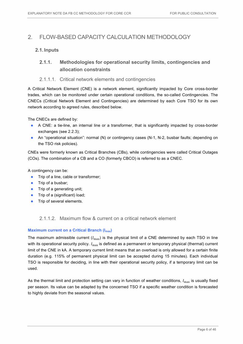
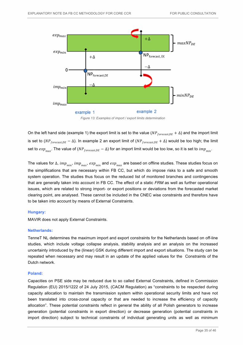
With respect to this reference the German export/import will be restricted to a safely acceptable level. An algorithm ensures that the values of the export/import limits are within a reasonable range. Figure 13 illustrates the determination of the export/import limits in more detail:

12 While the text refers to Germany for the sake of readability, the area of Luxemburg is also covered by this External Constraint.


of 46

Figure 13: Examples of import / export limits determination

On the left hand side (example 1) the export limit is set to the value (𝑁𝑃𝑓𝑜𝑟𝑒𝑐𝑎𝑠𝑡,𝐷𝐸 + ∆) and the import limit

is set to (𝑁𝑃𝑓𝑜𝑟𝑒𝑐𝑎𝑠𝑡,𝐷𝐸 − ∆). In example 2 an export limit of (𝑁𝑃𝑓𝑜𝑟𝑒𝑐𝑎𝑠𝑡,𝐷𝐸 + ∆) would be too high; the limit

set to 𝑒𝑥𝑝𝑚𝑎𝑥. The value of (𝑁𝑃𝑓𝑜𝑟𝑒𝑐𝑎𝑠𝑡,𝐷𝐸 − ∆) for an import limit would be too low, so it is set to 𝑖𝑚𝑝𝑚𝑖𝑛.

The values for ∆, 𝑖𝑚𝑝𝑚𝑖𝑛, 𝑖𝑚𝑝𝑚𝑎𝑥, 𝑒𝑥𝑝𝑚𝑖𝑛 and 𝑒𝑥𝑝𝑚𝑎𝑥 are based on offline studies. These studies focus on

the simplifications that are necessary within FB CC, but which do impose risks to a safe and smooth system operation. The studies thus focus on the reduced list of monitored branches and contingencies that are generally taken into account in FB CC. The effect of a static FRM as well as further operational issues, which are related to strong import- or export positions or deviations from the forecasted market clearing point, are analysed. These cannot be included in the CNEC wise constraints and therefore have to be taken into account by means of External Constraints.

Hungary:

MAVIR does not apply External Constraints.

Netherlands:

TenneT NL determines the maximum import and export constraints for the Netherlands based on off-line studies, which include voltage collapse analysis, stability analysis and an analysis on the increased uncertainty introduced by the (linear) GSK during different import and export situations. The study can be repeated when necessary and may result in an update of the applied values for the Constraints of the Dutch network.

Poland:

Capacities on PSE side may be reduced due to so called External Constraints, defined in Commission Regulation (EU) 2015/1222 of 24 July 2015, (CACM Regulation) as “constraints to be respected during capacity allocation to maintain the transmission system within operational security limits and have not been translated into cross-zonal capacity or that are needed to increase the efficiency of capacity allocation”. These potential constraints reflect in general the ability of all Polish generators to increase generation (potential constraints in export direction) or decrease generation (potential constraints in import direction) subject to technical constraints of individual generating units as well as minimum


of 46

reserve margins required in the whole Polish power system to ensure secure operation. This is related to the fact that under the conditions of central dispatch market model applied in Poland responsibility of Polish TSO on system balance is significantly extended comparing to such standard responsibility of TSO in self dispatch market models – see further explanations in this respect. Thus, capacity in export direction is reduced if the export of the PSE exceeds generating capacities left available within Polish power system taking into account necessary reserve margin for upward regulation. Similarly, capacity in import direction is reduced if the import exceeds downward regulation available within Polish power system taking into account necessary reserve margin for downward regulation.

Rationale behind implementation of allocation constraints on PSE side

Implementation of allocation constraints on PSE side is related to the fact that under the conditions of central dispatch market model applied in Poland responsibility of Polish TSO on system balance is significantly extended comparing to such standard responsibility of TSO in self dispatch market models. The latter is usually defined up to hour ahead time frame (including real time operations), while for PSE as Polish TSO this is extended to short (intraday and day ahead) and medium (up to year ahead) terms. Thus, PSE bears the responsibility, which in self dispatch markets is allocated to Balance Responsible Parties (BRPs). That is why PSE needs to take care of back up generating reserves for the whole Polish power system, which sometimes lead to implementation of allocation constraints if this is necessary to ensure operational security of Polish power system in terms of available generating capacities for upward or downward regulation. In self dispatch markets BRPs themselves are supposed to take care about their generating reserves, while TSO shall ensure them just for dealing with contingencies in the time frame of up to one hour ahead. Thus these two approaches ensure similar level of feasibility of transfer capacities offered to the market from the generating capacities point of view. It is worthwhile to note that infeasibilities in this respect lead to counter trade actions and appear only if faults out of dimensioning criteria occur. In order to better explain the above issue the following subchapters elaborate more on the differences between central and self-dispatch market models as well as on PSE’s role in system balancing.

Central vs self-dispatch market models

Market operation in Europe is carried out in several different ways. However, they can be basically grouped in two families: self-dispatch model and central-dispatch model. In a self-dispatch market, market design produces a balance between generation and demand (including external exchanges) by requiring that market parties (Balance Responsible Parties - BRPs) are in a balanced position to participate in the balancing market (e.g. one hour before energy delivery). Imbalance charges/penalties are levied on market parties which deviate from the balanced position. Commitment decisions, which take into account generating unit constraints, are made by the generators in conjunction with the demand elements they are balancing with. Generators alter their output to maintain the balance between generation and served demand. To be able to maintain balanced position they keep the given amount of reserves in their internal portfolios for compensation of their deviations. Before real time, generators submit bids to TSO which correspond with self-schedules of their units. Bids are used by TSO to dispatch additional generation needed to balance and secure the system in real time. Most of the electricity markets in Europe are based on the self-dispatch principle.


of 46

In a central dispatch market, in order to provide generation and demand balance, the TSO dispatches generating units taking into account their operational constraints, transmission constraints and reserve requirements. This is realized in an integrated process as an optimisation problem called Security Constrained Unit Commitment and Economic Dispatch (SCUC/ED). The main distinguishing feature of a central dispatch model is that balancing, congestion management and reserve procurement are performed simultaneously and they start day before and continuing until real time. This involves dispatch instructions being issued several hours ahead of real time, to start up units (SCUC), as well as real time instructions for dispatching on line units (SCED). In central dispatch model market participants do not need to be in a balanced position. The existing central-dispatch markets in Europe currently are the Greek, the Italian, the Irish and the Polish electricity markets.

PSE role in system balancing

PSE directly dispatches generating units taking into account their operational constraints and transmission constraints in order to cover the expected load having in mind adequate reserve requirements, which is also forecasted by PSE itself. To fulfil this task PSE runs the process of operational planning, which begins three years ahead with relevant overhaul (maintenance) coordination and is continued via yearly, monthly and weekly updates to day ahead security constrained unit commitment (SCUC) and economic dispatch (SCED). The results of this day ahead market are then updated continuously in intraday time frame up to real time operation. In a yearly timeframe PSE tries to distribute the maintenance overhauls requested by generators along the year in such a way that on average the minimum year ahead reserve margin of 18% (over forecasted load including already allocated capacities on interconnections, if any) is kept on average in each month. The monthly and weekly updates aim to keep this reserve margin on each day at the level of 17% and 14% respectively, if possible. This process includes also network maintenance planning, so any constraints coming from the network operation are duly taken into account. The day ahead SCUC process aims to achieve 9% of spinning reserve (or quickly activated, in Polish reality only units in pumped storage plants) margin for each hour of the next day. This includes primary and secondary control power pre-contracted as an ancillary service. The rest of this reserve comes from usage of balancing bids, which are mandatory to be submitted by all centrally dispatched generating units (in practice all units connected to the transmission network and major ones connected to 110 kV, except CHP plants as they operate mainly according to heat demand). The other generation is taken into account as scheduled by owners, which having in mind its stable character (CHPs, small thermal and hydro) is workable solution. The only exception from this rule is wind generation, which due to its volatile character is forecasted by PSE itself (like a system demand) and relevant uncertainty margins are included (90% for yearly and monthly time horizons referring to installed generation and 20% day ahead referring to forecasted generation). Thus, PSE has the right to use any available centrally dispatched generation in normal operation to balance the system. The negative reserve requirements during low load periods (night hours) are also respected and the potential pumping operation of pumped storage plants is taken into account, if feasible. The further updates of SCUC/SCED during the operational day take into account any changes happening in the system (forced outages and any limitations of generating units and network elements, load and wind forecast updates, etc.) and aim to keep at minimum 7% of spinning reserve for each hour


of 46

(as described above) in a time frame corresponding to the start-up times of the remaining thermal generating units (in practice 6 to 8 hours). Such an approach usually allows to keep one hour ahead spinning reserve at the minimum level of 1000 MW (i.e. potential loss of the largest generating unit of 850 MW and 150 MW of primary control reserve being PSE’s share in RGCE).

Practical determination of allocation constraints within the Polish power system

As an example the process of practical determination of allocation constraints in the framework of day ahead transfer capacity calculation is illustrated on the below figures 14 and 15. They illustrate how a forecast of the Polish power balance for each hour of the next day is developed by TSO day ahead in the morning in order to find reserves in generating capacities available for potential exports and imports, respectively. Allocation constraint in export direction occurs if generating capacities left available on centrally dispatched units within Polish power system for export are lower than the sum of export ATCs on all three interconnections (synchronous cross section, Swepol Link and Litpol Link). Allocation constraint in import direction occurs if downward regulating capacities left available on centrally dispatched units in operation within Polish power system for imports (ΔImport) are lower than the sum of import ATCs on all three interconnections (synchronous cross section, Swepol Link and Litpol Link).


of 46

1. sum of available generating capacities of centrally dispatched units13 as declared by generators, reduced by: 1.1 TSO forecast of capacity not available due

to expected network constraints 1.2 TSO assessment (based on experiences

of recent days) of extra reserve to cover short term unavailabilities not declared by generators day ahead (limitations coming from e.g. cooling conditions, fuel supply, etc.) and prolonged overhauls and/or forced outages

2. sum of schedules of generating units that are not centrally dispatched as provided by generators, except wind farms for which generation is forecasted by TSO

3. load forecasted by TSO 4. minimum necessary reserve for up regulation

(for day ahead: 9% of forecasted load)

Figure 14: Determination of allocation constraints in export direction (reserves in generating capacities available for potential exports) in the framework of day ahead transfer capacity calculation

13 note that generating units, which have very limited working hours left due to environmental restrictions are not taken into account in power balance

for determining export allocation constraints: most of these units are still in operation only thanks to special contracts with TSO (thus being out of the

market) – otherwise they would have already been decommissioned as not profitable; currently also all pumped storage units in Poland are also

operated by TSO out of market (for the same reason), however these units are taken into account in power balance for determining export allocation

constraints as their operation is not limited environmentally


of 46

1 TSO estimation of sum of technical minima of centrally dispatched generating units in operation

2 sum of schedules of generating units that are not centrally dispatched as provided by generators, except wind farms for which TSO forecast of wind generation is taken into account

3 load forecasted by TSO 3.1 minimum necessary reserve for down

regulation (for day ahead: 500MW)

Figure 15: Determination of allocation constraints in import direction (reserves in generating capacities available for potential imports) in the framework of day ahead transfer capacity calculation

Romania:

Transelectrica determines export and import limits based on off-line half-yearly studies for stability issues and daily analysis for a minimum level of operational reserve.

Slovakia:

External Constraints in form of exp/imp limit may be introduced subject to operational security assessment results.

Slovenia:

ELES does not apply External Constraints.


of 46

APPENDIX 2 - Methods for GSKs per bidding zone

The following section depicts in detail the method currently used by each Core TSO to design and implement GSKs.

Austria:

APG’s method only considers market driven power plants in the GSK file which was done with statistical analysis of the market behaviour of the power plants. This means that only pump storages and thermal units are considered. Power plants which generate base load (river power plants) are not considered. Only river plants with daily water storage are also taken into account in the GSK file. The list of relevant power plants is updated regularly in order to consider maintenance or outages. Furthermore the GSK file will also be updated seasonally because in the summer period the thermal units are out of operation.

Belgium:

Elia will use in its GSK flexible and controllable production units which are available inside the Elia grid (they can be running or not). Units unavailable due to outage or maintenance are not included. The GSK is tuned in such a way that for high levels of import into the Belgian bidding zone all units are, at the same time, either at 0 MW or at Pmin (including a margin for reserves) depending on whether the units have to run or not (specifically for instance for delivery of primary or secondary reserves). For high levels of export from the Belgian bidding zone all units are at Pmax (including a margin for reserves) at the same time. After producing the GSK, Elia will adjust production levels in all 24 hour D2CF to match the linearised level of production to the exchange programs of the reference day as illustrated in Figure 16.

Figure 16: Belgian GSK.

Max exportMax import 0

Pmax

Pmin


of 46

Croatia:

HOPS will use in its GSK all flexible and controllable production units which are available inside the HOPS’ grid (mostly hydro units). Units unavailable due to outage and maintenance are not included, but units that aren’t currently running are included in GSK. Due to different grid operation in each season of the year GSK will be updated accordingly.

Czech Republic:

The Czech GSK considers all production units which are available inside CEPS´s grid and were foreseen to be in operation in target day. Units planned for the maintenance are not included in the GSK file. The list of GSK is produced on hourly basis. The generation pattern inside GSK is shifted proportionally to the given Pgen. The current approach of creation GSKs is regularly analysed and can be adapted to reflect actual situation in CEPS´s grid.

Netherlands:

TenneT B.V. will dispatch the main generators in such a way as to avoid extensive and not realistic under- and overloading of the units for extreme import or export scenarios. Unavailability due to outages are considered in the GSK. Also the GSK is directly adjusted in case of new power plants. All GSK units (including available GSK units with no production in de D2CF file) are redispatched pro rata on the basis of predefined maximum and minimum production levels for each active unit. The total production level remains the same. The maximum production level is the contribution of the unit in a predefined extreme maximum production scenario. The minimum production level is the contribution of the unit in a predefined extreme minimum production scenario. Base-load units will have a smaller difference between their maximum and minimum production levels than start-stop units.

France:

The French GSK is composed of all the units connected to RTE’s network in the D-2 CGM. The variation of the generation pattern inside the GSK is the following: all the units which are in operation in the D-2 CGM will follow the change of the French net position based on the share of their nominal productions. In other words, if one unit represents n% of the total generation on the French bidding zone, n% of the shift of the French net position will be attributed to this unit.

Germany:

The German14 TSOs provide one single GSK for the whole German bidding zone. Since the structure of the generation differs for each German TSO, an approach has been developed, which allows the single TSO to provide GSKs that respect the specific character of the generation in their own grid while ultimately yielding a comprehensive single German GSK. In a first step, each German TSO creates a TSO-specific GSK with respect to its own control area based on its local expertise. The TSO-specific GSK denotes how a change of the net position in the forecasted market clearing point of the respective TSO’s control area is distributed among the nodes of this area.

14 The area of Luxemburg is taken into account in the contribution from Amprion.


of 46

This means that the nodal factors of each TSO-specific GSK add up to 1. Details of the creation of the TSO-specific GSKs are given below per TSO. In a second step, the four TSO-specific GSK are combined into a single German GSK by assigning relative weights to each TSO-specific GSK. These weights reflect the distribution of the total market driven generation among German TSOs. The weights add up to 1 as well. With this method, the knowledge and experience of each German TSO can be brought into the process to obtain a representative GSK. As a result, the nodes in the GSK are distributed over whole Germany in a realistic way, and the individual factors per node are relatively small. Both the TSO-specific GSKs and the TSOs’ weights are time variant and updated on a regular basis. Clustering of time periods (e.g. peak hours, off-peak hours, week days, weekend days) may be applied for transparency and efficiency reasons.

Individual distribution per German TSO

50Hertz:

The GSKs for the control zone of 50Hertz are based on a regular statistical assessment of the behaviour of the generation park for various market clearing points. In addition to the information on generator availability, the interdependence with fundamental data such as date and time, season, wind infeed etc. is taken into account. Based on these, the GSKs for every MTU are created.

Amprion:

Amprion established a regular process in order to keep the GSK as close as possible to the reality. In this process Amprion checks for example whether there are new power plants in the grid or whether there is a block out of service. According to these monthly changes in the grid Amprion updates its GSK. If needed Amprion adapts the GSK in meantime during the month. In general Amprion only considers middle and peak load power plants as GSK relevant. With other words basic load power plants like nuclear and lignite power plants are excluded to be a GSK relevant node. From this it follows that Amprion only takes the following types of power plants: hard coal, gas and hydro power plants. In the view of Amprion only these types of power plants are taking part of changes in the production.

TenneT Germany:

Similar to Amprion, TTG considers middle and peak load power plants as potential candidates for GSK. This includes the following type of production units: coal, gas, oil and hydro. Nuclear power plants are excluded upfront. In order to determine the TTG GSK, a statistical analysis on the behavior of the non-nuclear power plants in the TTG control area has been made with the target to characterize the units. Only those power plants, which are characterized as market-driven, are put in the GSK. This list is updated regularly.

TransnetBW:

To determine relevant generation units TransnetBW takes into account the power plant availability and the most recent available information at the time when the individual GSK-file is generated for the MTU:


of 46

The GSK for every power plant i is determined as:

𝐺𝑆𝐾! = 𝑃!"#,! − 𝑃!"#,!𝑃!"#,! − 𝑃!"#,!!

!!!

Equation 15

Where n is the number of power plants, which are considered for the generation shift within TransnetBW’s control area. Only those power plants which are characterized as market-driven, are used in the GSK if their availability for the target hour is known. The following types of generation units for middle and peak load connected to the transmission grid can be considered in the GSK: l hard coal power plants l hydro power plants l gas power plants

Nuclear power plants as baseload units are excluded because of their mostly constant infeed.

Hungary:

MAVIR uses general GSK file listing all possible nodes to be considered in shifting the net position in a proportional way, i.e. in the ratio of the actual generation at the respective nodes. All dispatchable units, including actually not running ones connected to the transmission grid are represented in the list. Furthermore, as the Hungarian power system has generally considerable import, not only big generation units directly connected to the transmission grid are represented, but small, dispersed ones connected to lower voltage levels as well. Therefore, all 120 kV nodes being modelled in the IGM are also listed representing this kind of generation in a proportional way, too. Ratio of generation connected to the transmission grid and to lower voltage levels is set to 50-50% at present.

Poland:

PSE present in GSK file all dispatchable units which were foreseen to be in operation in day of operation. Units planned for the maintenance are not included on the list. The list is created for each hour. The generation pattern listed in the GSK is changed proportionally to the given Pgen.

Romania:

The Transelectrica GSK file contains all dispatchable units which are available in the day of operation. The units planned for maintenance and nuclear units are not included in the list.

Slovakia:

In GSK file of SEPS are given all dispatchable units which are in operation in respective day and hour which the list is created for. The units planned for maintenance and nuclear units are not included in the list. All mentioned nodes to be considered in shifting the net position in a proportional way.

Slovenia:

GSK file of ELES consists of all the generation nodes specifying those generators that are likely to contribute to the shift. Nuclear units are not included in the list. In additional also load nodes that shall contribute to the shift are part of the list in order to take into account the contribution of generators connected to lower voltage levels (implicitly contained in the load figures of the nodes connected to the


of 46

220 and 400 kV grid). At the moment GSK file is designed according to the participation factors, which are the result of statistical assessment of the behaviour of the generation units infeeds.


of 46

APPENDIX 3 - Determination of threshold for CNEC selection

The threshold will be set following security assessments performed by TSOs, by the iterative process described below: TSOs will carry out some alternative computations of flow-based parameters, using scenarios where only the threshold is set to different values. Depending of the threshold values, some Critical Network Elements are included or not in the flow-based parameters computation, resulting in a capacity domain more or less constraining for the market. Taking some extreme “vertices” of the resulting alternative Flow-Based domains, TSOs will assess whether these domains are safe, and more precisely identify at which point the exclusion of CNE not respecting the threshold would lead to unacceptable situations, with respect to Core TSOs risk policies. If for one given threshold value, the analyses would conclude in unacceptable situations (because the removal of some constraints would allow an amount of exchanges that TSOs could not cope with as they would not respect standard Security of Supply (SOS) principles, like the standard N-1 rule), then this simply means that the threshold is too high. Following this approach and assessing different values, Core TSOs should conclude which X% is an optimal compromise, in terms of size of the domain versus risk policies.