explaining the cross-section of share returns in …

UNIVERSITY OF KWAZULU-NATAL

EXPLAINING THE CROSS-SECTION OF SHARE RETURNS

IN SOUTH AFRICA USING MACROECONOMIC FACTOR

MODELS

AILIE CHARTERIS

This thesis is submitted in fulfilment of the requirements of the degree Doctor of

Philosophy (Finance)

School of Accounting, Economics and Finance

College of Law and Management Studies

Pietermaritzburg Campus

SUPERVISOR: PROFESSOR J. FAIRBURN

CO-SUPERVISOR: MR B. STRYDOM

2016

ii

DECLARATION

I, Ailie Charteris, declare that:

(i) The research reported in this dissertation, except where otherwise indicated, is my

original research.

(ii) This dissertation has not been submitted for any degree or examination at any other

university.

(iii) This dissertation does not contain other persons’ data, pictures, graphs or other

information, unless specifically acknowledged as being sourced from other persons.

(iv) This dissertation does not contain other persons’ writing, unless specifically

acknowledged as being sourced from other researchers. Where other written sources

have been quoted then:

Their words have been re-written but the general information attributed to them

has been referenced;

Where the exact words have been used, their writing has been placed inside

quotation marks and properly referenced.

(v) Where I have reproduced a publication of which I am the author, co-author or editor,

l have indicated in detail which part of the publication was written by me alone.

(vi) This dissertation does not contain any text, graphics or tables copied from other

internet sources, unless specifically acknowledged, with the source being written out

in the dissertation and bibliography section.

Signed: …………………………………. Date: …………………………………….

iii

ACKNOWLEDGEMENTS

I am never one who is short of words, but I am at a loss as to how to sufficiently express my

gratitude to so many people for their guidance and support throughout this very long journey.

To my supervisors, Jim and Barry, thank you for your insights, motivation and always being there

to act as a sounding board for my thoughts. Your impact on me extends far beyond this thesis.

To friends and colleagues who have always been there with an encouraging word, a hug or to

share ideas with – thank you!

Mum and Dad, I would never have completed this without you – I have been blessed beyond

words to have such loving and supportive parents.

Thank you Lord for your countless blessings and sustaining me throughout.

“The joy of the Lord is my strength”

Nehemiah 8:10.

iv

ABSTRACT

Understanding asset prices is critical for the decision-making of many; from professional and

individual investors, who seek to earn the highest possible return from their investments, to

governments and corporates evaluating investment and consumption choices. Given that the

behaviour of asset prices may differ across countries, especially across varying levels of

development, applying knowledge of the determinants of asset prices from one country to another

may not be appropriate.

Asset pricing models can typically be grouped into one of two categories – portfolio or

macroeconomic. The principle focus of this study is on models which fall under the latter

grouping, where little research has been conducted on the South African market. These models

are concerned with identifying the true risk factors which drive share returns, in contrast to

portfolio-based models, which simply measure risk as the sensitivity of a share’s returns to

portfolios of securities. The consumption-based capital asset pricing model (CAPM), which links

consumption to investor behaviour in their demand for securities, provides the foundation for the

majority of the macroeconomic models. Labour income and household wealth are seen as two

critical measures that are linked to the consumption decisions of investors and several models

which have incorporated these two factors are evaluated in this study. In particular, those of Lettau

and Ludvigson (2001b), Piazzesi, Schneider, and Tuzel (2003, 2007), Lustig and van

Nieuwerburgh (2005), Santos and Veronesi (2006) and Yogo (2006) are examined to assess their

ability to explain the size and value anomalies on the Johannesburg Stock Exchange (JSE). The

results are compared to several portfolio-based models including the CAPM, the conditional

CAPM and the Fama and French (1993) three-factor model. The models are tested over the period

June 1990 to April 2013 using a comprehensive sample of JSE-listed shares based on the Fama

and MacBeth (1973) and generalised method of moments methods.

The study finds that many of the macroeconomic models are less successful in explaining returns

of South African shares compared to the developed markets which have been examined

internationally. However, there is weak evidence to suggest that returns are correlated with factors

which capture how investors’ returns vary with labour income, housing wealth and consumption.

In particular, value shares earn higher returns than growth shares partly to compensate investors

for greater risk in the macroeconomy where risk is captured by the interaction of consumption,

asset wealth and labour income, while small shares are more sensitive to shocks in housing

scarcity thus partially accounting for their higher returns compared to larger shares. The results

of this study are analysed in conjunction with the international evidence so as to consider possible

reasons for the weaker results obtained and the implications for understanding the factors that

drive assets prices are reviewed. Finally, suggestions for future research are provided.

v

TABLE OF CONTENTS

DECLARATION ......................................................................................................................... ii

ACKNOWLEDGEMENTS ....................................................................................................... iii

ABSTRACT ................................................................................................................................ iv

TABLE OF CONTENTS ............................................................................................................ v

LIST OF TABLES ...................................................................................................................... x

LIST OF FIGURES .................................................................................................................. xii

LIST OF ACRONYMS ........................................................................................................... xiii

Chapter 1 : THE SCOPE AND PURPOSE OF THIS STUDY ............................................... 1

1.1 BACKGROUND AND PROBLEM DEFINITION ..................................................... 1

1.1.1 Measuring Risk........................................................................................................ 1

1.1.2 Alternative Asset Pricing Models........................................................................... 3

1.1.3 Research Problem ................................................................................................... 8

1.1.4 Research Objectives ................................................................................................ 8

1.2 DATA AND METHOD OF THE STUDY .................................................................... 9

1.2.1 Delineation of the Study .......................................................................................... 9

1.2.2 The Scope of the Study ......................................................................................... 10

1.2.3 Research Methodology .......................................................................................... 10

1.3 STRUCTURE OF THE STUDY .................................................................................. 12

Chapter 2 : A REVIEW OF THE CAPM THEORY AND EVIDENCE ............................. 14

2.1 INTRODUCTION ......................................................................................................... 14

2.2 THE THEORETICAL BASIS OF THE CAPM ........................................................ 14

2.2.1 MPT and the CAPM ............................................................................................. 15

2.2.2 The SDF Framework ............................................................................................ 19

2.2.2.1 The SDF Approach to Asset Pricing ................................................................... 19

2.2.2.2 The SDF and Beta Pricing Models ..................................................................... 21

2.2.2.3 The SDF for the CAPM ....................................................................................... 23

2.3 EMPIRICAL TESTS OF THE CAPM ....................................................................... 24

2.3.1 Joint Tests of the CAPM and Market Efficiency ............................................... 24

2.3.2 Methodological Considerations ............................................................................ 25

2.3.3 Early Empirical Tests ........................................................................................... 26

2.3.4 The Size and Value Anomalies ............................................................................. 29

2.3.5 Explanations for the Anomalies ........................................................................... 32

2.3.6 The CAPM in South Africa .................................................................................. 35

2.3.6.1 Initial Tests of the CAPM and Segmentation on the JSE .................................... 35

2.3.6.2 The Size and Value Anomalies on the JSE .......................................................... 37

2.4 RESEARCH PROBLEM AND DATA ....................................................................... 38

2.4.1 Research Problem ................................................................................................. 38

2.4.2 Time Period............................................................................................................ 39

2.4.3 Share Price Data .................................................................................................... 39

2.4.3.1 Data Considerations ........................................................................................... 39

2.4.3.2 Share Inclusions and Exclusions ......................................................................... 39

2.4.3.3 Treatment of Corporate Actions .......................................................................... 40

2.4.3.4 Liquidity Filter .................................................................................................... 42

2.4.4 Share Returns ........................................................................................................ 42

vi

2.4.5 Portfolio Formation .............................................................................................. 43

2.4.5.1 Size- and Value-Sorted Portfolios ....................................................................... 44

2.4.5.2 Industry-Sorted Portfolios ................................................................................... 47

2.4.6 The Computation of the Pricing Factors ............................................................. 48

2.5 METHODOLOGY ........................................................................................................ 49

2.5.1 Time-Series Regressions ....................................................................................... 49

2.5.2 Cross-Sectional Regressions ................................................................................. 51

2.5.3 GMM in Asset Pricing Tests ................................................................................ 56

2.5.3.1 An Introduction to GMM ..................................................................................... 56

2.5.3.2 Using GMM to Estimate the SDF ....................................................................... 58

2.5.3.3 Estimation Considerations .................................................................................. 61

2.6.1 Descriptive Statistics of the Portfolios ................................................................. 63

2.6.2 Time-Series Regression Results ........................................................................... 68

2.6.3 Cross-Sectional Regression Results ..................................................................... 72

2.6.4 GMM Regression Results ..................................................................................... 78

2.7 CONCLUSION .............................................................................................................. 78

Chapter 3 : PORTFOLIO AND MACROECONOMIC ASSET PRICING MODELS ..... 80

3.1 INTRODUCTION ......................................................................................................... 80

3.2 TIME-VARYING ASSET PRICING MODELS ....................................................... 81

3.2.1 Time-Series Predictability of Returns ................................................................. 81

3.2.1.1 Empirical Evidence of Predictability .................................................................. 81

3.2.1.2 Methodological Limitations as an Explanation for Predictability ...................... 83

3.2.1.3 Reconciling Time-Series Predictability with Theory........................................... 84

3.2.1.4 Time-Series Predictability and Business Cycles ................................................. 87

3.2.1.5 Time-Series Predictability in South Africa .......................................................... 88

3.2.2 The Intertemporal CAPM .................................................................................... 88

3.2.3 The Conditional CAPM ........................................................................................ 91

3.2.3.1 The Conditional CAPM of Jagannathan and Wang (1996) ................................ 91

3.2.3.2 The Conditional CAPM in the SDF Framework ................................................. 94

3.2.3.3 Empirical Tests of the Conditional CAPM .......................................................... 96

3.2.3.4 Conclusions Regarding the Conditional CAPM ................................................. 98

3.3 OTHER MULTIFACTOR PRICING MODELS ...................................................... 98

3.3.1 The APT ................................................................................................................. 98

3.3.2 The Fama and French (1993) Three-Factor Model ......................................... 101

3.4 THE CONSUMPTION CAPM .................................................................................. 104

3.4.1 The Derivation of the Consumption CAPM ..................................................... 104

3.4.2 Empirical Tests of the Consumption CAPM .................................................... 109

3.4.3 Conclusions Regarding the Consumption CAPM ............................................ 110

3.5 ANALYSIS .................................................................................................................. 111

3.5.1 Research Problem ............................................................................................... 111

3.5.2 Predicting the Market Risk Premium ............................................................... 112

3.5.3 The Computation of the Pricing Factors ........................................................... 116

3.5.3.1 The Conditional CAPM ..................................................................................... 116

3.5.3.2 The Fama and French (1993) Three-Factor Model .......................................... 116

3.5.3.3 The Consumption CAPM ................................................................................... 117

3.5.4 Methodology ........................................................................................................ 118

3.5.4.1 Traded versus Non-Traded Factors .................................................................. 118

3.5.4.2 The Conditional CAPM .................................................................................... 120

vii

3.5.4.3 Estimating Multifactor Models ........................................................................ 121

3.6 RESULTS .................................................................................................................... 122

3.6.1 Time-Series Predictability of the Market Risk Premium ................................ 122

3.6.2 The Conditional CAPM ...................................................................................... 127

3.6.2.1 Cross-Sectional Regression Results .................................................................. 127

3.6.2.2 GMM Regression Results .................................................................................. 133

3.6.3 The Fama and French (1993) Three-Factor Model ......................................... 135

3.6.3.1 Time-Series Regression Results ........................................................................ 135



3.6.4 The Consumption CAPM ................................................................................... 143



3.7 CONCLUSION ............................................................................................................ 148

Chapter 4 : THE ROLE OF LABOUR INCOME IN ASSET PRICING .......................... 150

4.1 INTRODUCTION ....................................................................................................... 150

4.2 LABOUR INCOME IN ASSET PRICING .............................................................. 151

4.2.1 The Importance of Human Capital ................................................................... 151

4.2.2 Measuring Human Capital ................................................................................. 153

4.2.3 Asset Pricing Models with Labour Income ....................................................... 154

4.2.4 Conditional Models with Scaling Factors that Include Labour Income ........ 158

4.2.4.1 Lettau and Ludvigson (2001b) .......................................................................... 158

4.2.4.2 Debate Surrounding the Validity of 𝑐𝑎𝑦 ........................................................... 165

4.2.4.3 Santos and Veronesi (2006) .............................................................................. 168

4.3 ANALYSIS .................................................................................................................. 172


4.3.2 Computation of the Pricing Factors .................................................................. 173

4.3.2.1 The CAPM with Labour Income........................................................................ 173

4.2.3.2 𝑐𝑎𝑦 .................................................................................................................... 175

4.3.2.3 𝑠𝑦 ....................................................................................................................... 180

4.3.3 Methodology ........................................................................................................ 180

4.4 RESULTS .................................................................................................................... 180

4.4.1 The CAPM with Labour Income ....................................................................... 181




4.4.2 The Conditional CAPM and (C)CAPM with 𝒄𝒂𝒚 ............................................ 188

4.4.2.1 Estimates of 𝑐𝑎𝑦 ................................................................................................ 188

4.4.2.2 Descriptive Statistics and the Predictive Power of 𝑐𝑎𝑦 .................................... 191



4.4.3 The Conditional CAPM and (C)CAPM with sy .............................................. 204

4.4.3.1 Descriptive Statistics and the Predictive Power of 𝑠𝑦 ...................................... 204

4.4.3.2 Cross-sectional Regression Results .................................................................. 208


4.4 CONCLUSION ............................................................................................................ 215

Chapter 5 : THE ROLE OF HOUSING WEALTH IN ASSET PRICING ....................... 217

5.1 INTRODUCTION ....................................................................................................... 217

viii

5.2 HOUSING WEALTH IN ASSET PRICING............................................................ 218

5.2.1 The Importance of Housing Wealth .................................................................. 218

5.2.2 The CAPM with Real Estate Wealth ................................................................. 220

5.2.3 Conditional Models with Scaling Factors that Include Housing Wealth ....... 223

5.2.3.1 Piazzesi et al. (2003, 2007) ............................................................................... 223

5.2.3.2 Lustig and van Nieuwerburgh (2005) ............................................................... 226

5.2.3.3 Sousa (2010)...................................................................................................... 230

5.3.3.3 Criticism of these Models .................................................................................. 231

5.2.4 The Durable CAPM ............................................................................................ 232

5.3 ANALYSIS .................................................................................................................. 234


5.3.2 Computation of the Pricing Factors .................................................................. 235

5.3.2.1 The Real Estate CAPM ...................................................................................... 235

5.3.2.2 CH-CAPM ......................................................................................................... 237

5.3.2.3 𝑚�� ..................................................................................................................... 237

5.3.2.4 The Durable CAPM ........................................................................................... 238

5.3.3 Methodology ........................................................................................................ 240

5.4 RESULTS .................................................................................................................... 240

5.4.1 The Real Estate CAPM and Real Estate CAPM with Labour Income .......... 241




5.4.2 The CH-CAPM .................................................................................................... 250

5.4.2.1 Descriptive Statistics and the Predictive Power of 𝛼 ........................................ 250



5.4.3 The Collateral CAPM ......................................................................................... 263

5.4.3.1 Estimates of my ................................................................................................. 263

5.4.3.2 Descriptive Statistics and the Predictive Power of 𝑚��..................................... 264



5.4.4 The Durable CAPM ............................................................................................ 273

5.4.4.1 Descriptive Statistics ......................................................................................... 273



5.5 CONCLUSION ............................................................................................................ 282

Chapter 6 : CONCLUSIONS AND RECOMMENDATIONS ........................................... 285

6.1 INTRODUCTION ....................................................................................................... 285

6.2 A REVIEW OF THE PROBLEM STATEMENT ................................................... 285

6.3 SUMMARY OF FINDINGS ...................................................................................... 287

6.3.1 The CAPM, the Two-Factor Model and the Three-Factor Model ................. 287

6.3.2 A Test of the Conditional CAPM on the JSE ................................................... 288

6.3.3 A Test of the Consumption CAPM on the JSE ................................................ 289

6.3.4 The Role of Labour Income in Explaining South African Share Returns ..... 290

6.3.5 The Role of Housing Wealth in Explaining South African Share Returns .... 291

6.4 CONCLUSION ............................................................................................................ 292

6.5 LIMITATIONS OF THE STUDY ............................................................................. 293

6.6 RECOMMENDATIONS FOR FUTURE RESEARCH .......................................... 295

ix

6.6.1 Further Research on Macroeconomic Factors ................................................. 295

6.6.2 Additional Opportunities for Further Research .............................................. 297

REFERENCES ........................................................................................................................ 299

APPENDIX .............................................................................................................................. 323

ETHICAL CLEARANCE ...................................................................................................... 341

x

LIST OF TABLES

Table 1-1: A Summary of a Selection of Asset Pricing Models ................................................. 4

Table 2-1: Characteristics of the Size and Value Portfolios ..................................................... 64

Table 2-2: Average Annual Number of Shares in the Industry Portfolios ................................ 66

Table 2-3: Descriptive Statistics of the Size and Value Portfolios ........................................... 67

Table 2-4: Descriptive Statistics of the Industry Portfolios ...................................................... 68

Table 2-5: Correlation Matrix of the Pricing Factors in the CAPM and Two-Factor Model ... 69

Table 2-6: Time-Series Estimates of the Factor Risk Premia for the CAPM and Two-Factor

Model ...................................................................................................................... 69

Table 2-7: Time-Series Regression Results for the CAPM and Two-Factor Model ................ 70

Table 2-8: Cross-Sectional Regression Results for the CAPM and Two-Factor Model ........... 73

Table 2-9: GMM Regression Results for the CAPM and Two-Factor Model .......................... 79

Table 3-1: Descriptive Statistics of the Excess Market Returns over Various Horizons ........ 122

Table 3-2: Summary Statistics of the Predictor Variables ...................................................... 123

Table 3-3: Forecasts of Multiple Quarter Excess Real Market Returns.................................. 124

Table 3-4: Cross-Sectional Regression Results for the Conditional CAPM ........................... 128

Table 3-5: GMM Regression Results for the Conditional CAPM .......................................... 134

Table 3-6: Correlation Matrix of the Pricing Factors in the CAPM and Two-Factor Model . 136

Table 3-7: Time-Series Estimates of the Factor Risk Premia for the Fama and French

(1993) Model ......................................................................................................... 136

Table 3-8: Time-Series Regression Results for the Fama and French (1993) Model ............. 137

Table 3-9: Cross-Sectional Regression Results for the Fama and French (1993) Model ....... 139

Table 3-10: GMM Regression Results for the Fama and French (1993) Model ...................... 142

Table 3-11: Descriptive Statistics of the Growth Rate in Consumption ................................... 143

Table 3-12: Cross-Sectional Regression Results for the Consumption CAPM ........................ 144

Table 3-13: GMM Regression Results for the Consumption CAPM ....................................... 148

Table 4-1: Correlation Matrix of the Excess Market Returns and Growth Rate in Labour

Income ................................................................................................................... 181

Table 4-2: Time-Series Estimates of the Factor Risk Premia for the CAPM with Labour

Income ................................................................................................................... 182

Table 4-3: Time-Series Regression Results for the CAPM with Labour Income ................... 183

Table 4-4: Cross-Sectional Regression Results for the CAPM with Labour Income ............. 184

Table 4-5: GMM Regression Results for the CAPM with Labour Income ............................ 188

Table 4-6: Estimates for the Components of cay .................................................................... 189

Table 4-7: Summary Statistics of cay ..................................................................................... 192

Table 4-8: Forecasts of Multiple Quarter Excess Real Market Returns using cay ................. 192

Table 4-9: Cross-Sectional Regression Results for the Conditional Models with cay ........... 196

Table 4-10: GMM Regression Results for the Conditional Models with cay ........................... 204

Table 4-11: Descriptive Statistics of sy .................................................................................... 205

Table 4-12: Forecasts of Multiple Quarter Excess Real Market Returns using sy ................... 207

Table 4-13: Cross-Sectional Regression Results for the Conditional Models with sy ............. 209

Table 4-14: GMM Regression Results for the Conditional Models with sy ............................. 213

Table 5-1: Correlation Matrix of the Pricing Factors in the Real Estate CAPM and Real

Estate CAPM with Labour Income ....................................................................... 241

Table 5-2: Time-Series Estimates of the Factor Risk Premia for the Real Estate CAPM

and Real Estate CAPM with Labour Income ........................................................ 242

Table 5-3: Time-Series Regression Results for the Real Estate CAPM and Real Estate

xi

CAPM with Labour Income ................................................................................... 243

Table 5-4: Cross-Sectional Regression Results for the Real Estate CAPM and Real Estate

CAPM with Labour Income ................................................................................... 245

Table 5-5: GMM Regression Results for the Real Estate CAPM and Real Estate CAPM

with Labour Income ............................................................................................... 250

Table 5-6: Summary Statistics of α ......................................................................................... 251

Table 5-7: Forecasts of Multiple Quarter Excess Real Market Returns using α ..................... 253

Table 5-8: Descriptive Statistics of the Non-Housing Consumption Growth Rate ................ 255

Table 5-9: Cross-Sectional Regression Results for the Collateral Housing Models ............... 256

Table 5-10: GMM Regression Results for the Collateral Housing Models .............................. 261

Table 5-11: Estimates for the Components of my .................................................................... 264

Table 5-12: Summary Statistics of my ...................................................................................... 265

Table 5-13: Forecasts of Multiple Quarter Excess Real Market Returns using my .................. 266

Table 5-14: Cross-Sectional Regression Results for the Collateral CAPM .............................. 268

Table 5-15: GMM Regression Results for the Collateral CAPM ............................................. 273

Table 5-16: Summary Statistics of the Stock of Durable Goods .............................................. 274

Table 5-17: Cross-Sectional Regression Results for the Durable CAPM with ∆d* .................. 276

Table 5-18: GMM Regression Results for the Durable CAPM with ∆d* ................................. 281

xii

LIST OF FIGURES

Figure 1-1: R100 Investment in a Portfolio of Small Firms and a Portfolio of Large Firms ...... 1

Figure 2-1: Average Quarterly Real Returns for the Size and Value Portfolios ....................... 66

Figure 2-2: CAPM Betas for the Size and Value Portfolios ..................................................... 74

Figure 2-3: Pricing Errors from the CAPM for the Size and Value Portfolios ......................... 77

Figure 3-1: Conditional CAPM Betas for the Size and Value Portfolios ............................... 131

Figure 3-2: Pricing Errors from the Conditional CAPM for the Size and Value Portfolios ... 133

Figure 3-3: Pricing Errors from the Fama and French (1993) Model for the Size and Value

Portfolios .............................................................................................................. 140

Figure 3-4: Consumption CAPM Betas for the Size and Value Portfolios ............................. 146

Figure 3-5: Pricing Errors from the Consumption CAPM for the Size and Value Portfolios . 147

Figure 4-1: The Ratio of Total Consumption to Consumption on Non-Durable Goods and

Services ................................................................................................................ 176

Figure 4-2: Labour Betas for the Size and Value Portfolios ................................................... 186

Figure 4-3: Pricing Errors for the CAPM with Labour Income for the Size and Value

Portfolios .............................................................................................................. 187

Figure 4-4: Excess Real Market Returns and cay ................................................................... 194

Figure 4-5: Conditional Consumption Betas using cay for the Size and Value Portfolios ..... 199

Figure 4-6: Conditional Consumption Betas using cay for High and Low B/M Portfolios in

Good and Bad States ............................................................................................ 200

Figure 4-7: Conditional Consumption Betas using cay for Small and Large Portfolios in

Good and Bad States ............................................................................................ 201

Figure 4-8: Pricing Errors from the (C)CAPM with cay for the Size and Value Portfolios ... 202

Figure 4-9: The Value of sy for South Africa ........................................................................ 206

Figure 4-10: Conditional Betas using sy for the Size and Value Portfolios ............................. 211

Figure 5-1: Residential Real Estate Betas from the Real Estate CAPM for the Size and

Value Portfolios ................................................................................................... 247

Figure 5-2: Pricing Errors from the Real Estate CAPM for the Size and Value Portfolios .... 248

Figure 5-3: The Value of α in South Africa ............................................................................ 252

Figure 5-4: Conditional Betas using α for the Size and Value Portfolios ............................... 258

Figure 5-5: Pricing Errors from the Conditional CH-CAPM for the Size and Value

Portfolios .............................................................................................................. 259

Figure 5-6: The Value of my for South Africa ....................................................................... 265

Figure 5-7: Conditional Betas using my for the Size and Value Portfolios ............................ 270

Figure 5-8: Pricing Errors from the Collateral CAPM with Non-Separable Preferences for

the Size and Value Portfolios ............................................................................... 271

Figure 5-9: Non-Contemporaneous Durable Consumption Betas Based on ∆d*for the Size

and Value Portfolios ............................................................................................. 279

Figure 5-10: Pricing Errors from the Non-Contemporaneous Durable CAPM with ∆d* for

the Size and Value Portfolios ............................................................................... 280

xiii

LIST OF ACRONYMS

ADF: Augmented Dickey-Fuller (1979) test

AIC: Akaike information criterion

ALSI: FTSE/JSE All Share Index (J203)

Alt-X: Alternative exchange

AMEX: American stock exchange

APT: Arbitrage pricing theory

𝐵/𝑀: Book-to-market ratio

BEA: Bureau of Economic Analysis

CAPM: Capital asset pricing model

𝑐𝑎𝑦: Consumption aggregate wealth ratio

𝑐𝑑𝑎𝑦: Consumption disaggregate wealth ratio

(C)CAPM: Conditional consumption capital asset pricing model

CH-CAPM: Collateral housing capital asset pricing model

CML: Capital market line

CPI: Consumer price index

DLS: Dynamic least squares

𝐷/𝑃: Dividend-to-price ratio (also known as the dividend yield)

𝐸/𝑃: Earnings-to-price ratio (also known as the earnings yield)

EMH: Efficient market hypothesis

FINDI: FTSE/ JSE Financial and Industrial Index (J250)

FTSE: Financial Times stock exchange

GDP: Gross domestic product

GLS: Generalised least squares

GMM: Generalised method of moments

GRS: Gibbons, Ross and Shanken (1989)

HJ: Hansen and Jagannathan (1997)

HML: High minus low 𝐵/𝑀 firms

ICB: International Classification Benchmark

IID: Independent and identically distributed

INET BFA: INET Bureau of Financial Analysis

JSE: Johannesburg stock exchange

KPSS: Kwiatkowski, Phillips, Schmidt and Shin (1992) test

ME: Maximum-eigenvalue

MPT: Modern portfolio theory

NYSE: New York stock exchange

xiv

NASDAQ: National association of securities dealers automated quotations

𝑚𝑦: Collateral housing ratio

𝑚��: Collateral scarcity ratio

OLS: Ordinary least squares

𝑃/𝐸: Price-to-earnings ratio

PLS: Property loan stock

PUT: Property unit trust

𝑅2: R-squared

��2: Adjusted R-squared

REIT: Real estate investment trust

RESI: FTSE/ JSE Resources Index (J210)

RMSE: Root mean squared error

SARB: South African Reserve Bank

SDF: Stochastic discount factor

SIC: Schwarz information criterion

SMB: Small minus big firms

SML: Security market line

𝑠𝑦: Labour income-to-consumption ratio

T-bill: Treasury bill

VAR: Vector autoregression

VECM: Vector error correction model

U.K: United Kingdom

U.S: United States

1

Chapter 1 : THE SCOPE AND PURPOSE OF THIS STUDY

1.1 BACKGROUND AND PROBLEM DEFINITION

1.1.1 Measuring Risk

Understanding asset prices is a critical issue for both professional investors and individuals who

wish to earn the highest possible return from their investments. Moreover, asset prices also

contain important information for macroeconomic decisions pertaining to investment and

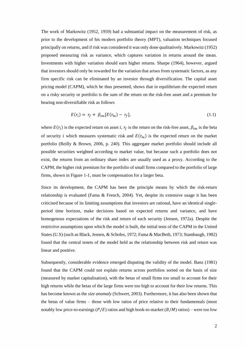
consumption (Campbell, 2014). Figure 1-1 depicts a R100 investment in a portfolio comprising

small South African firms and a portfolio of large South African firms over the period January

2003 to March 2013. As can be seen, the investment in the portfolio of small firms yielded a

substantially higher value at the end of the period, with a return equivalent to 46% per annum,

compared to 13% per annum from the investment in the portfolio of large firms. This higher return

should be a reward for the greater risk of holding small firms - a concept often referred to as the

first principle of finance (Ghysels, Santa-Clara, & Valkanov, 2005). The existence of a higher

risk premium for some firms raises the question of how risk differs across shares and accordingly

how risk is measured.

Figure 1-1: R100 Investment in a Portfolio of Small Firms and a Portfolio of Large Firms

This figure tracks a R100 investment in a diversified portfolio comprising small South African firms and a

diversified portfolio comprising large South African firms (where size is measured by market capitalisation)

over a ten-year period commencing in quarter one of 2003. Both portfolios have approximately the same

book-to-market ratio. At the end of quarter one in 2013, the R100 investment in the portfolio of small firms

was worth R559 while that in the portfolio of large firms was worth R234 equating to an annual return of

45.85% and 13.37% respectively.

2

The work of Markowitz (1952, 1959) had a substantial impact on the measurement of risk, as

prior to the development of his modern portfolio theory (MPT), valuation techniques focused

principally on returns, and if risk was considered it was only done qualitatively. Markowitz (1952)

proposed measuring risk as variance, which captures variation in returns around the mean.

Investments with higher variation should earn higher returns. Sharpe (1964), however, argued

that investors should only be rewarded for the variation that arises from systematic factors, as any

firm specific risk can be eliminated by an investor through diversification. The capital asset

pricing model (CAPM), which he thus presented, shows that in equilibrium the expected return

on a risky security or portfolio is the sum of the return on the risk-free asset and a premium for

bearing non-diversifiable risk as follows

𝐸(𝑟𝑖) = 𝑟𝑓 + 𝛽𝑖𝑚[𝐸(𝑟𝑚) − 𝑟𝑓], (1.1)

where 𝐸(𝑟𝑖) is the expected return on asset 𝑖, 𝑟𝑓 is the return on the risk-free asset, 𝛽𝑖𝑚 is the beta

of security 𝑖 which measures systematic risk and 𝐸(𝑟𝑚) is the expected return on the market

portfolio (Reilly & Brown, 2006, p. 240). This aggregate market portfolio should include all

possible securities weighted according to market value, but because such a portfolio does not

exist, the returns from an ordinary share index are usually used as a proxy. According to the

CAPM, the higher risk premium for the portfolio of small firms compared to the portfolio of large

firms, shown in Figure 1-1, must be compensation for a larger beta.

Since its development, the CAPM has been the principle means by which the risk-return

relationship is evaluated (Fama & French, 2004). Yet, despite its extensive usage it has been

criticised because of its limiting assumptions that investors are rational, have an identical single-

period time horizon, make decisions based on expected returns and variance, and have

homogenous expectations of the risk and return of each security (Jensen, 1972a). Despite the

restrictive assumptions upon which the model is built, the initial tests of the CAPM in the United

States (U.S) (such as Black, Jensen, & Scholes, 1972; Fama & MacBeth, 1973; Stambaugh, 1982)

found that the central tenets of the model held as the relationship between risk and return was

linear and positive.

Subsequently, considerable evidence emerged disputing the validity of the model. Banz (1981)

found that the CAPM could not explain returns across portfolios sorted on the basis of size

(measured by market capitalisation), with the betas of small firms too small to account for their

high returns while the betas of the large firms were too high to account for their low returns. This

has become known as the size anomaly (Schwert, 2003). Furthermore, it has also been shown that

the betas of value firms – those with low ratios of price relative to their fundamentals (most

notably low price-to-earnings (𝑃/𝐸) ratios and high book-to-market (𝐵/𝑀) ratios) – were too low

3

to account for their high returns, with the opposite true for growth firms, which have high prices

relative to their fundamentals (Basu, 1977; Stattman, 1980; Rosenberg, Reid, & Lanstein, 1985).

This phenomenon is known as the value anomaly. Fama and French (1992) confirmed that these

anomalies are separate effects and, additionally, they found that the positive relationship between

beta and returns predicted by the CAPM was flat in practice. The emergence of this evidence

disputing the validity of the model thus raised questions about the suitability of the CAPM as a

description of the risk-return relationship for the U.S market (Fama & French, 2004).

Similar findings have been documented in markets outside of the U.S (Fama & French, 1998),

including South Africa (van Rensburg & Robertson, 2003b; Basiewicz & Auret, 2009; Strugnell,

Gilbert, & Kruger, 2011; Ward & Muller, 2012). Furthermore, in South Africa a negative

relationship between beta and returns has been identified, which contradicts the first principle of

finance that higher risk should be compensated with higher returns (van Rensburg & Robertson,

2003b; Strugnell et al., 2011; Ward & Muller, 2012). Accordingly, the CAPM is not suitable for

explaining differences in risk premia across shares listed on the Johannesburg stock exchange

(JSE). These points can be simply illustrated by returning to the example in Figure 1-1. The

CAPM betas for the portfolio of small firms and large firms were 0.61 and 1.03 respectively for

the period. The higher return associated with the portfolio of small firms was thus not

commensurate with a higher level of risk which is evidence of the size anomaly. Moreover, the

fact that the beta of the small firm portfolio was lower than that of the large firm portfolio

contradicts the positive risk-return relationship that theory implies.

The CAPM is often termed a “portfolio-based model” (Cochrane, 2008a, p. 241), as the risk of

the security, measured by beta, is determined by the sensitivity of the security returns to a portfolio

of securities. In fact, one of the substantive criticisms of the model is that it does not address what

factors explain the returns on the securities in the market portfolio and accordingly, does not

actually answer the fundamental question of what influences the risk premium (Cochrane, 2005,

pp. xiv).

Given the limiting assumptions of the CAPM, its poor empirical performance, and the fact that it

reveals little about what factors determine share returns, the model is not considered to provide

an appropriate description of the risk-return relationship (Cochrane, 2008a). Consequently,

considerable research has focused on the identification of a model that can provide a more suitable

measure of risk.

1.1.2 Alternative Asset Pricing Models

Several models which have been developed as alternatives to the CAPM for understanding the

risk-return relationship are summarised in Table 1-1. The standard means of measuring the

4

empirical worth of an asset pricing model has been its ability to explain the size and value premia

by examining the R-squared (𝑅2), adjusted for degrees of freedom (��2) of a cross-sectional

regression of 25 size- and value-sorted portfolios (value is normally measured by the 𝐵/𝑀 ratio).

As noted in Table 1-1, the CAPM has only been able to explain approximately 1% of the variation

across these portfolios.

Table 1-1: A Summary of a Selection of Asset Pricing Models

Study Model ��𝟐

Panel A: Portfolio-based Models

Jagannathan and Wang (1996);

Lettau and Ludvigson (2001b)

CAPM 1%

Lettau and Ludvigson (2001b) Fama and French (1993) three-factor model 80%

Jagannathan and Wang (1996) Conditional CAPM with the default spread as

the conditioning variable

30%#

Jagannathan and Wang (1996) Conditional CAPM with labour income 55%

Kullmann (2003); Funke, Gebken,

Johanning, and Michel (2010)

CAPM with real estate 49%

Panel B: Macroeconomic-based Models

Breeden (1979) Consumption CAPM 16%

Lettau and Ludvigson (2001b) (C)CAPM with a conditioning variable

capturing the interaction between labour

income, consumption and asset wealth

70%

Piazzesi et al. (2003) Conditional CAPM with a conditioning

variable capturing composition risk between

consumption on housing services and non-

housing goods and services

82%

Lustig and van Nieuwerburgh

(2005)

(C)CAPM with a conditioning variable

capturing the interaction housing wealth,

labour income and consumption

88%

Santos and Veronesi (2006) Conditional CAPM with a conditioning

variable capturing the interaction between

labour income and consumption

57%

Yogo (2006) Durable CAPM which includes durable and

non-durable consumption

94%

This table provides details of a selection of asset pricing models which can be classified as either portfolio-

or macroeconomic-based models. Under the former classification, the factors which determine the returns

of the security are synthesised portfolios of securities, whereas under the latter, various macroeconomic

factors explain share returns. These models have been tested in cross-sectional regressions on the 25 size-

and value-sorted portfolios on the U.S. market, with their explanatory power, as measured by ��2, shown.

# This study used size and beta-sorted portfolios rather than the size- and value-sorted portfolios.

In light of the limiting assumptions underpinning the CAPM, several models have sought to relax

these assumptions so as to provide a more accurate description of reality. The conditional CAPM,

initially proposed by Jagannathan and Wang (1996) and extended by Lettau and Ludvigson

(2001b), is one such example. This model expands the single-period time horizon by allowing for

5

the possibility that both returns and risk may vary over business cycles. The variation in the

parameters is captured through a variable which is able to closely predict business cycles, such as

the default spread or dividend-to-price ratio (𝐷/𝑃). As shown in Table 1-1, this model does

provide a notable improvement on the CAPM, but is still only able to explain a third of the cross-

sectional variation in share returns.

Fama and French (1993) proposed a three-factor model that was derived directly from the inability

of the CAPM to explain the size and value anomalies and, as such, does not have any theoretical

foundation. The factors are the market return, the return on a portfolio capturing the size premium

and the return on a portfolio capturing the value premium, with Fama and French (1993)

suggesting that these two additional factors proxy for risk not captured by beta. This model has

been shown to explain between 55% and 80% of the cross-sectional variation in returns of the 25

size and 𝐵/𝑀 sorted portfolios, which is far higher than the CAPM. This model has also been

found to be successful in several other markets including the United Kingdom (U.K) (Bagella,

Becchetti, & Carpentieri, 2000) and Australia (Brailsford, Gaunt, & O’Brien, 2012). Basiewicz

and Auret (2010) also found that the Fama and French (1993) model provided a more accurate

description of the risk premium associated with small and value shares on the JSE than either the

CAPM or two-factor model, which accounts for the segmented nature of the South African

market1. In light of this success, Fama and French (2004) recommended the model as a viable

alternative to the CAPM, as do texts such as Cuthbertson and Nitzsche (2005:199), terming it the

current ‘market leader’ in explaining returns. Basiewicz and Auret (2010) drew the same

conclusion for evaluating risk and return on the JSE. However, this model has been criticised due

to the absence of a theoretical basis as it is entirely motivated by empirical findings (Davis, Fama

& French, 2000).

The theoretically derived conditional CAPM and the empirically motivated three-factor model,

similarly to the CAPM, can be classified as portfolio-based models, as their additional sources of

risk merely capture the sensitivity of the security’s returns to the returns of synthesised portfolios.

As such, these two models are still subject to the same criticism as the CAPM that they do not

provide any information about the actual determinants of share returns. Macroeconomic variables

are considered as candidate factors for the determinants of share returns as it is well-documented

that share returns respond to external forces (Chen, Roll, & Ross, 1986). The arbitrage pricing

theory (APT) of Ross (1976) is an asset pricing model which enables the direct links between

macroeconomic variables and share returns to be examined. It provides a very general framework

1 van Rensburg and Slaney (1997) and van Rensburg (2002) identified two distinct underlying factors on

the JSE allied to the resources and financials/ industrials segments. Given that resources tend to respond

differently to market-wide risks, van Rensburg (2002) proposed a two-factor model with a resources index

and financials/industrials index so as to more accurately capture the risk associated with the two segments.

6

as it makes no assumptions about investor behaviour, with the pricing equation instead arising as

a result of arbitrage (through the law of one price). As such, the model yields a generic pricing

equation but with no information on the factors that actually influence returns. In this regard,

macroeconomic variables are viewed as strong candidate factors as they should affect aggregate

returns (a requirement of the model). However, despite providing a framework for the evaluation

of the link between the macroeconomy and share returns, this model has not formed the

foundation of recent work in asset pricing. This trend can be attributed to the fact that researchers

are not concerned about whether a particular macroeconomic variable (such as industrial

production or exchange rates) influences aggregate returns, as per the APT, but rather whether

the macroeconomic variable affects the behaviour of investors in their demand for securities.

In this regard, the consumption CAPM of Breeden (1979), which links the macroeconomy to the

utility investors derive from returns, has gained considerable traction and forms the cornerstone

of the recent developments in macroeconomic-based asset pricing. The consumption CAPM is

built on the assumption that rational risk-averse investors will seek to maximise their lifetime

utility and as such, it does not rely on the limiting assumptions of the CAPM of mean-variance

utility or a single period investment horizon. In this model, the risk of a security is measured as

the sensitivity of the security’s returns to the growth rate in aggregate consumption. Despite the

fact that the model has a strong theoretical underpinning and overcomes several of the limitations

of the standard CAPM, it only performs marginally better in terms of its ability to explain the

variation in the size and value portfolios, as shown in Table 1-1. One possible reason for the poor

performance of the model is that aggregate consumption is not directly observable and thus the

proxy used may not adequately capture risk.

Considerable work in understanding the determinants of share returns in the macroeconomic

framework has focused on the role of human capital (measured by labour income) and the wealth

arising from home ownership. However, the original literature pertaining to these factors

originated in the CAPM framework with the goal of providing a more encompassing measure of

the market portfolio than an ordinary share index provides. Jagannathan and Wang (1996), for

example, incorporated labour income, while Kullmann (2003) and Funke et al. (2010) included

returns from real estate. These studies showed that shares which were more correlated with the

returns to labour income and housing and commercial property earned higher returns.

Further developments in incorporating labour income and housing wealth into asset prices has

been tied into the consumption framework. The ability of an individual to consume goods and

services in the current and future periods is affected by their human capital and as such,

consumption patterns are likely to vary over time in response to variations in human capital. This

in turn will affect asset prices, because if a security pays out when returns to human capital are

7

low, the security will provide greater marginal utility than a security which pays out when returns

to human capital are high. The capital gains from an investment in housing can also be used to

fund consumption while the services derived from housing can be substituted with consumption

on non-housing goods and services. Empirical tests have confirmed that consumption, labour

income, housing wealth and share returns are linked (Lettau & Ludvigson, 2001a; Piazzesi et al.,

2003; Lustig & van Nieuwerburgh, 2005; Santos & Veronesi, 2006; Sousa, 2010).

Under the consumption CAPM, security prices are assumed to only be influenced by the

consumption of non-durable goods and services and not directly by other potential sources of

utility. Thus, any effects arising from human capital or housing wealth should be incorporated

into the consumption measure. However, the proxy used for aggregate consumption may not

adequately capture the relationships between consumption, human capital and housing wealth. In

light of this shortcoming, Lettau and Ludvigson (2001a) derived a model that included the risk

arising from the interaction between consumption, labour income and share returns using the

composite variable they derived as a conditioning variable. Thus, their model not only

incorporated risk arising from human capital but also allowed for the possibility of time-varying

risk and return, in the spirit of the conditional CAPM. They termed the model they derived the

conditional consumption CAPM, denoted (C)CAPM. Piazzesi et al. (2003), Lustig and van

Nieuwerburgh (2005) and Santos and Veronesi (2006) tested similar models. The major

difference between these specifications is the conditioning variables which capture different

aspects of the relationship between consumption, labour income, housing wealth and share

returns, as detailed in Table 1-1. As the results show, these models have been able to account for

a substantial component of the cross-sectional variation in the size and value portfolios. Finally,

Yogo (2006) developed a model focusing on consumption from durable goods, which, similarly

to housing provide service flows for more than one quarter. On the basis of ��2, this model yielded

the highest explanatory power of those listed.

The question of the most suitable measure of risk to explain differences in returns across securities

is not a simple one as it depends upon the criterion that is used as the basis for the choice - is a

‘good’ asset pricing model one which simply performs well or one which sheds light on what

factors actually drive asset returns and consequently performs well? Certainly, while the Fama

and French (1993) model may explain the risk premia associated with small and value shares, it

does not meet the second criterion as it provides no information about the underlying factors

which explain differences in returns. Cochrane (2005, pp. xiv) highlighted macroeconomic

variables as candidate determinants of asset prices and consistent with this, the macroeconomic

factor models highlighted not only perform well empirically but also provide information about

the factors that drive share returns. Despite the successes these models have achieved, Cochrane

(2005, pp. xiv) noted that this task of identifying the appropriate macroeconomic variables is not

8

yet complete, with the on-going research in this area a testament to the fact that a single

encompassing model has yet to be identified. Despite this, however, models such as that of Lettau

and Ludvigson (2001b) have been proposed as a viable alternative to the use of the Fama and

French (1993) three-factor model in well-respected texts on asset pricing such as Cochrane

(2005).

1.1.3 Research Problem

Studies have long-documented the failure of the CAPM to explain the risk-return relationship for

South African shares. While the Fama and French (1993) model appears to provide a reasonably

valid description of risk premia on small and value firms on the JSE, the model lacks any

underlying theory and accordingly, provides no satisfactory information as to what factors

actually determine share returns on this emerging market.

The identity of an asset pricing model which performs well and can explain the determinants of

share returns is of critical importance for both finance and macroeconomics (Cochrane, 1996),

where the central focus is on whether macroeconomic variables affect the behaviour of investors

(through the consumption CAPM) in their demand for securities and not simply whether the

variable affects share returns in aggregate (as would be the case under the APT). As mentioned

previously, Cochrane (2005, pp. xiv) refers to the identification of these macroeconomic drivers

of investor behaviour and thus share returns as a yet unfinished task. Part of this incomplete work

can be seen as ascertaining whether the factors which have been found to be important in the U.S

(and a few other, mostly developed, countries) in the research to date, are applicable to other

markets, especially those with differing levels of development, institutions and practices. Despite

the importance thereof, no attempts have been made to consider how labour income and housing

wealth as macroeconomic risks drive share prices, via their impact on investor behaviour, on the

JSE. Therefore, this study focuses on addressing part of the unfinished task of macroeconomic

asset pricing by evaluating whether factors that have been found to drive investor behaviour and

thus asset prices on the U.S market are applicable to the emerging market of South Africa. The

research question can thus be summarised as:

Can macroeconomic models incorporating labour income and housing wealth explain the cross-

section of share returns in South Africa?

1.1.4 Research Objectives

The detailed research objectives of the study are as follows:

9

To conduct an updated examination of the suitability of the CAPM, van Rensburg’s

(2002) two-factor model (to account for segmentation on the JSE) and Fama and

French’s (1993) three-factor model to explain the size and value anomalies on the JSE.

To test whether the conditional CAPM, which allows for time-variation in risk and

return, can explain the cross-sectional variation in South African share returns.

To examine the suitability of the consumption CAPM in explaining the cross-sectional

variation in size- and value-sorted portfolios of JSE-listed shares.

To consider whether the inclusion of the relationship between labour income,

consumption and share returns in the consumption CAPM can explain the cross-sectional

variation in South African share returns.

To determine whether the adaptation of the consumption CAPM to account for the

interaction between housing wealth, consumption and share returns (and in some cases

labour income) can explain the size and value anomalies on the JSE.

To ascertain whether the durable CAPM can explain the cross-sectional variation in

share returns in South Africa.

1.2 DATA AND METHOD OF THE STUDY

1.2.1 Delineation of the Study

Rather than testing asset pricing models with individual securities, portfolios of securities were

favoured, as this helps to circumvent several empirical problems that arise with the use of

individual assets. A variety of attributes have been employed as the basis for this grouping, but

given that the empirical worth of models internationally has been assessed by their ability to

explain the variation in returns of size- and value-sorted portfolios, similar portfolios were formed

on the basis of both size and the 𝐵/𝑀 ratio. Lewellen, Nagel, and Shanken (2010) argued that a

model must be able to explain all patterns in the data, not only the size and value phenomena.

Accordingly, the analysis was supplemented with a set of portfolios sorted on industry

classifications.

The momentum effect is one of the most researched anomalies alongside size and value. This

anomaly, first documented by Jegadeesh and Titman (1993), refers to the short-term persistence

in returns where shares which have performed well in the past one to 12 months continue to

perform well up to a year thereafter, while those that have performed poorly continue to perform

poorly. Although some scholars have ascribed this anomaly to the inability of the CAPM to

explain returns (Griffin, Ji, & Martin, 2003), as is the case with the size and value anomalies, the

phenomenon has been widely attributed to the behavioural biases of investors (Barberis, Shleifer,

10

& Vishny, 1998; Hong & Stein, 1999). For example, the slow reaction to news by investors means

that past performance is extrapolated giving rise to momentum in share returns. Given the strong

behavioural-based explanations that have been proffered for the momentum anomaly, this

particular pattern in share returns was not considered in this study which focuses on a risk-based

explanation for the anomalies.

Closely allied to momentum is the mean-reversion phenomenon identified by De Bondt and

Thaler (1985). They found that shares that had performed well in the past three to five years

tended to perform poorly in the following three to five years, while the reverse was true for the

firms that had performed poorly in the past. This anomaly is principally attributed to behavioural

biases in the decision-making of investors (Cubbin, Eidne, Firer, & Gilbert, 2006, pp. 39); most

notably that of overreaction and hence is often termed the overreaction anomaly (De Bondt &

Thaler, 1985). Although this explanation for mean-reversion in stock prices appears to contradict

the under-reaction description proffered for short-term persistence in returns, the models of

Barberis et al. (1998) and Daniel, Hirshleifer, and Subrahmanyam (1998) do account for the

possibility that investors under-react to information in the short-run but overreact in the longer-

term. In light of the evidence that mean reversion is largely attributed to irrational investor

behaviour, this anomaly, similarly to momentum, is not examined in this study.

1.2.2 The Scope of the Study

This study covers the period January 1990 to April 2013 and included all ordinary shares listed

on the main board of the JSE. Accessing data prior to 1990 for shares listed on the JSE is difficult,

as noted in several studies (van Rensburg & Robertson, 2003b; Strugnell et al., 2011). All shares

listed at any point during this period were included thus accounting for firms which delisted and

were newly listed during the sample period. Adjustments were made for corporate actions such

as share splits, acquisitions and name changes. Price, dividend and relevant accounting data was

gathered for all shares from INET Bureau of Financial Analysis (BFA). Traditionally monthly

share price data has been used for asset pricing tests; but the inclusion of economic variables,

which are only released quarterly, as pricing factors meant that quarterly data was employed.

1.2.3 Research Methodology

As indicated, several tests of the ability of the CAPM and van Rensburg’s (2002) two-factor

model to explain returns of size and value portfolios have been conducted on the JSE, while

Basiewicz and Auret (2010) conducted a test of the Fama and French (1993) three-factor model.

However, an updated test of these three models was performed not only to provide a basis of

comparison against which the alternative models could be compared, but also to provide greater

insight into the cross-sectional dynamics of the models, as the tests thereof have predominantly

11

focused on the time-series implications. The single period horizon on which the CAPM is built is

limiting and thus the natural extension to an intertemporal framework established in the

conditional CAPM represents a potentially valuable alternative asset pricing model. This model,

which has not previously been tested on the South African market, was thus examined to ascertain

whether time-variation in both risk and return could account for the pricing anomalies.

As an alternative to these portfolio-based models, the consumption CAPM was also evaluated, as

this model represents the cornerstone of the macroeconomic approach to asset pricing. The

consumption CAPM has only ever been examined in the context of the equity premium puzzle on

the JSE (Hassan & van Biljon, 2010). Building on this framework, the risk arising from the

interconnectedness of labour income and consumption, which may not be fully captured in the

consumption CAPM, was examined using the models proposed by Lettau and Ludvigson (2001b)

and Santos and Veronesi (2006). The simple model of Jagannathan and Wang (1996) was also

tested as the initial examination of the role of labour income in asset pricing. In a similar manner,

the impact of the risk arising from the relationship between housing wealth and consumption (and

labour income) on the risk-return trade-off was evaluated using the models of Piazzesi et al.

(2003) and Lustig and van Nieuwerburgh (2005), with the initial examination of the role of

housing wealth on security prices conducted using the model of Kullmann (2003) and Funke et

al. (2010). The model of Yogo (2006) evaluates consumption expenditure on durable goods,

which are assets that provide service flows for more than one quarter, much like housing, but

whose value depreciates over time as the good is consumed which is not true for housing. Given

the success of this model, it was also examined.

Tests of asset pricing models are usually conducted in either the time-series or cross-sectional

frameworks. Time-series tests, however, can only be applied to models where the factors are

traded (Cochrane, 2005, pp. 235) and their appropriateness is also questioned in models which

allow for time-varying risk and return (Lewellen & Nagel, 2006). As such, the cross-sectional

method is more common, which was the primary focus of this study. But, given that time-series

regressions have to be estimated in order to obtain inputs for the cross-sectional regressions,

where appropriate, the tests were conducted as not only do they provide additional insight into

the suitability of the models but also enabled comparisons to be conducted to previous studies on

the JSE and several international studies where this approach has been used. These time-series

tests entailed testing the significance of the intercept in the regression (individually and jointly),

as these indicate the pricing error of the model for each portfolio. In addition to this, following

the original method of Black et al. (1972), the factor risk premia based on the time-series

information was also computed as the sample average.

12

Cross-sectional tests involve estimating the factor loadings for each portfolio against the portfolio

returns. However, due to common sources of variation in the portfolios, the residuals from this

regression are likely to be correlated, which biases the standard errors of the coefficients. To

account for this, the foremost method employed in international studies of Fama and MacBeth

(1973) was implemented. This method avoids the problem of the residual correlation through

repeated sampling. An additional adjustment was performed to these standard errors, following

Shanken (1992), so as to account for the fact that the factor loadings were estimates from

regressions and thus subject to error. The ability of the model to explain the size and value

anomalies was assessed based on ��2, the signs and significance of the risk premia, and tests of

significance of the cross-sectional pricing errors.

In order to ensure the reliability of the results obtained from the cross-sectional regression results,

the generalised method of moments (GMM) was also used to test the models. GMM can be used

to estimate the time-series and cross-sectional regressions, but in addition to this, it can also be

applied to estimate the stochastic discount factor (SDF) of an asset pricing model (Cochrane,

2005, pp. 187). The latter provides a natural fit to the framework in which many of the recent

models of asset pricing have been developed and was thus implemented. The signs and

significance of the parameters in the SDF were examined as well as the J-test of over-identifying

restrictions to test whether the pricing errors from the model were significant.

1.3 STRUCTURE OF THE STUDY

The remainder of the chapters in this study are structured as follows:

Chapter 2 – A Review of the CAPM Theory and Evidence: In this chapter an overview of the

CAPM is provided, from its derivation through to the anomalous patterns in share returns which

the model cannot explain. The suitability of the CAPM for pricing South African shares is

assessed so as to provide a basis of comparison for alternative models.

Chapter 3 – Portfolio and Macroeconomic Asset Pricing Models: Several portfolio-based

asset pricing models are critically examined, with particular attention on the conditional CAPM

and the Fama and French (1993) three-factor model. The consumption CAPM, which represents

the building block of macroeconomic factor models, is introduced. Several of the models

reviewed are tested on the JSE data to assess their appropriateness.

Chapter 4 – The Role of Labour Income in Asset Pricing: The relationship between labour

income, consumption and share returns is reviewed in this chapter. The theoretical and empirical

performance of asset pricing models which have been developed to incorporate this relationship

13

are then discussed; following which these models are tested to assess their ability to price

securities on the JSE.

Chapter 5 – The Role of Housing Wealth in Asset Pricing: In this chapter, the association

between housing wealth, consumption and share returns is discussed. Several studies which have

developed measures to account for the risk arising from this relationship in asset pricing models

are reviewed and thereafter, these models are tested to assess their suitability in explaining the

size and value anomalies on the JSE.

Chapter 6 – Conclusions and Recommendations: The findings of the study are summarised

and recommendations for future research based on the results are provided.

14

Chapter 2 : A REVIEW OF THE CAPM THEORY AND EVIDENCE

2.1 INTRODUCTION

The development of the CAPM by Sharpe (1964) and Lintner (1965a) revolutionised thinking on

the risk-return trade-off. While the initial tests of the CAPM generally supported its central tenets,

in subsequent examinations various anomalies began to emerge as differences in beta could not

explain differences in returns across assets with particular characteristics. Moreover, these

failures of the CAPM were not only germane to the U.S, but were identified in a number of other

developed and developing countries, including South Africa. Various explanations have been

proposed to account for these phenomena with some arguing that these anomalies arise because

investors are not always rational, while others contend that these anomalies indicate that the

CAPM is flawed. This chapter briefly reviews the theoretical foundation of this important model

in the context of Markowitz’s (1952) portfolio theory, with the more general SDF approach to

asset pricing introduced thereafter with application to the CAPM. The empirical tests of the ability

of the model to explain the risk-return relationship in various markets are reviewed, with

particular focus on the size and value anomalies.

Despite its well-documented limitations, the CAPM still plays a vital role in the asset pricing

literature as it provides the basis from which many alternative models have been developed.

Although the CAPM has been tested previously on the JSE (van Rensburg & Robertson, 2003b;

Basiewicz & Auret, 2010; Strugnell et al., 2011; Ward & Muller, 2012), the model is examined

so as to provide a basis of comparison against which the alternative models tested in the following

chapters of this study could be compared. Moreover, this analysis also offers new insights into

the cross-sectional dynamics of the model in explaining returns of JSE-listed shares, where only

limited statistical tests have been conducted previously, while also using a different testing

procedure and a different set of test assets. To only examine the CAPM however, would entail

ignoring the resources-financial/industrials dichotomy on the JSE which may give rise to incorrect

beta estimates. The two-factor model of van Rensburg (2002), which accounts for this

segmentation, is thus also evaluated. The data and methodology employed in this study to test

these two models is discussed, with the results and analysis presented thereafter.

2.2 THE THEORETICAL BASIS OF THE CAPM

The CAPM was derived from Markowitz’s (1952, 1959) MPT, which focuses on the relationship

between the expected return of an asset and its risk, as measured by variance. In the section that

15

follows, a brief derivation of the model is provided to facilitate understanding of the CAPM.

Thereafter the SDF framework for asset pricing is reviewed and applied to the CAPM.

2.2.1 MPT and the CAPM

MPT relies on several simplifying assumptions, including that investors are rational, risk-averse,

expected utility maximisers and that all investors have an identical single-period time horizon

(Jensen, 1972a). In addition, investors are assumed to choose portfolios on the basis of the

expected mean and variance of returns, with all investors having homogeneous expectations

thereof. Over and above the assumptions regarding investor behaviour, it is also assumed that

unlimited borrowing and lending can occur at the risk-free rate, that markets are perfect meaning

that there is perfect competition, there are no transaction costs, taxes or any other market frictions,

and all assets are marketable (Sharpe, 1964; Goltz & Le Sourd, 2011).

Markowitz (1952) plotted all risky securities and all possible combinations thereof, which

represents the investment opportunity set, on a plane of expected returns against standard

deviation2. The upper boundary of this opportunity set is termed the efficient frontier, as it plots

the securities/portfolios which have the highest expected return for each level of risk (Jensen,

1972a). Principally, the efficient frontier will comprise portfolios rather than individual assets

because combining securities together in a portfolio enables security specific risk to be reduced

through diversification (Sharpe, 1964). Given the assumption that investors have homogeneous

expectations, all investors will face the same efficient frontier. Rational investors will choose to

hold portfolios that plot on the efficient frontier as they provide the highest level of return for a

given level of risk (or alternatively, the lowest level of risk for a given level of return) (Markowitz,

1952). However, where the investor plots along the efficient frontier will depend on their

individual risk preferences, which are depicted graphically in the risk-return plane by their

indifference curves (Sharpe, 1964).

Tobin (1958) demonstrated that the introduction of a risk-free asset expands the opportunity set.

Every investor will now be able to hold a combination of an efficient risky portfolio and a risk-

free asset to achieve a desired risk-return trade-off. These combinations will lie along a straight-

line (known as a capital allocation line) connecting the risk-free asset and the risky portfolio in

the mean-standard deviation plane (Jensen, 1972a). A combination of the risk-free asset and the

portfolio where the capital allocation line is tangential to the efficient frontier will dominate all

other capital allocation lines, as on this line a higher return can be achieved for a given level of

risk than was obtainable with only risky assets in the opportunity set (Sharpe, 1964). Thus, any

point along this line is preferable to the original efficient frontier and investors will thus choose

2 Standard deviation is the square root of the variance.

16

combinations of the risk-free asset and tangential risky portfolio rather than the risky portfolio

only. This new efficient frontier is known as the capital market line (CML), with all assets plotting

along this line in equilibrium, otherwise there would be no demand for the security (Jensen,

1972a).

As all investors face the same efficient frontier because of their homogenous expectations, all

investors will thus hold the same portfolio; where they plot along the CML, however, will reflect

their personal risk preferences (determined by their indifference curves) (Sharpe, 1964). If an

investor is more risk-averse, they will hold a greater proportion of their portfolio in the riskless

asset while those more risk-loving investors may choose to borrow at the risk-free rate to enable

an even greater investment in the portfolio of risky assets (a leveraged position). The assertion

that all investors will first select the optimum risky portfolio and thereafter make a separate choice

of how to allocate their funds between this portfolio and the riskless asset was termed the two-

fund separation theorem by Tobin (1958). It demonstrates that an investor’s choice of the optimal

portfolio of risky assets is independent of their risk preferences.

If all investors hold the same portfolio of risky assets, then the portfolio must represent the market

portfolio consisting of all assets in exactly the proportion of that asset’s fraction to the total value

of all assets, otherwise any asset not included in the portfolio would have no demand (Fama &

French, 2004). Therefore, the pricing equation for any portfolio which plots on the CML is

𝐸(𝑟𝑒) = 𝑟𝐹 + (𝐸(𝑟𝑚)−𝑟𝐹)

𝜎𝑚*𝜎𝑒, (2.1)

where 𝐸(𝑟𝑒) is the expected return on an efficient portfolio and 𝜎𝑚 and 𝜎𝑒 are the standard

deviation of the market and efficient portfolio returns respectively (Sharpe, 1964, p. 438).

From this foundation provided by Markowitz (1952) and Tobin (1958), Sharpe (1964) sought to

determine the appropriate pricing equation for an individual asset. He argued that only the

systematic risk of a security should be rewarded, as investors should not be compensated for

bearing unnecessary asset specific (unsystematic) risk which can be diversified away by holding

the security as part of a well-diversified portfolio. Sharpe (1964) demonstrated the impact of this

risk distinction for the pricing of individual securities using a framework of two risky assets3: an

3 Jensen (1972a) showed an alternative way of deriving the CAPM using the two-fund separation theorem

but the same pricing formulation is obtained irrespective of the approach used.

17

individual risky security (denoted asset i) with a weighting of 𝛼 and the market portfolio, with a

weighting of (1 − 𝛼).4 The expected return of this portfolio can be written as

𝐸(𝑟𝑝) = 𝛼𝐸(𝑟𝑖) + (1 − 𝛼)𝐸(𝑟𝑚), (2.2)

and its risk as

𝜎𝑝 = {𝛼2𝜎𝑖2 + (1 − 𝛼)2𝜎𝑚

2 + 2𝛼(1 − 𝛼)𝑐𝑜𝑣(𝑟𝑖, 𝑟𝑚)}1/2, (2.3)

where 𝐸 denotes the unconditional expectations operator, 𝐸(𝑟𝑝) and 𝜎𝑝 are the expected return

and standard deviation of the portfolio, 𝜎𝑖 is the standard deviation of the returns of asset i and

𝑐𝑜𝑣(𝑟𝑖, 𝑟𝑚) is the covariance between the returns of asset i and the market portfolio (adapted from

Sharpe, 1964, p. 438).

The expected return and risk for a marginal change in 𝛼 are

𝑑𝐸(𝑟𝑝)

𝑑𝛼= 𝐸(𝑟𝑖) − 𝐸(𝑟𝑚), (2.4)

and

𝑑𝜎𝑝

𝑑𝛼=

1

2(𝛼2𝜎𝑖

2 + (1 − 𝛼)2𝜎𝑚2 + 2𝛼(1 − 𝛼)𝑐𝑜𝑣(𝑟𝑖, 𝑟𝑚))

−1

2∗ (2𝛼𝜎𝑖

2 − 2𝜎𝑚2 + 2𝛼𝜎𝑚

2

+𝑐𝑜𝑣(𝑟𝑖, 𝑟𝑚) − 4𝛼𝑐𝑜𝑣(𝑟𝑖, 𝑟𝑚)) (2.5)

(Sharpe, 1964, p. 438; van der Wijst, 2013, p. 72). From 2.3, the first term in the derivative in 2.5

can be substituted with 1

𝜎𝑝 and simplifying gives the following

𝑑𝜎𝑝

𝑑𝛼=

𝛼(𝜎𝑖2+𝜎𝑚

2 −𝑐𝑜𝑣(𝑟𝑖,𝑟𝑚))+𝑐𝑜𝑣(𝑟𝑖,𝑟𝑚)−𝜎𝑚2

𝜎𝑝 . (2.6)

On the original efficient frontier, at the optimal portfolio, all funds are invested in the market

portfolio, so that the derivative can be evaluated at the point where 𝛼 = 0 and 𝜎𝑝 will be equal to

𝜎𝑀. Thus, equation 2.6 can be simplified as

𝑑𝜎𝑝

𝑑𝛼=

𝑐𝑜𝑣(𝑟𝑖,𝑟𝑚)−𝜎𝑚2

𝜎𝑚 (2.7)

(Sharpe, 1964, p. 438). From 2.4 and 2.7, the slope of the expected return-risk trade-off can be

written as

4 This portfolio is inefficient as the optimal portfolio is one where all shares should be held in proportion

to their market value, whereas in this combination, asset i, which is already included in the market portfolio,

is allocated a greater weighting.

18

𝐸(𝑟𝑝)

𝑑𝜎𝑝=

[𝐸(𝑟𝑖)−𝐸(𝑟𝑚)]∗𝜎𝑚

𝑐𝑜𝑣(𝑟𝑖,𝑟𝑚)−𝜎𝑚2 . (2.8)

At this point, the slope is equal to the slope of the tangential CML (as per equation 2.1)

[𝐸(𝑟𝑖)−𝐸(𝑟𝑚)]𝜎𝑚

𝑐𝑜𝑣(𝑟𝑖,𝑟𝑚)−𝜎𝑚2 =

[𝐸(𝑟𝑚)−𝑟𝐹]

𝜎𝑚, (2.9)

and rearranging yields the well-known CAPM formulation (as per equation 1.1), which can be

used to price individual securities and portfolios

𝐸(𝑟𝑖) = 𝑟𝐹 + 𝛽𝑖𝑚[𝐸(𝑟𝑚) − 𝑟𝐹], (2.10)

where 𝛽𝑖𝑚 =𝑐𝑜𝑣(𝑟𝑖,𝑟𝑚)

𝜎𝑚2 and represents a measure of systematic risk (van der Wijst, 2013, p. 73).

Beta measures the sensitivity of returns to a portfolio of assets (the market portfolio) and is thus

known as a portfolio-based asset pricing model (Cochrane, 2008a, pp. 240). The security market

line (SML) provides a graphical depiction of the relationship between beta and returns.

As is evident, the risk-free asset plays a critical role in the derivation of the CAPM. Black (1972)

however, showed that if the assumption of the existence of riskless rate at which investors can

both borrow and lend is violated, Tobin’s (1958) two-fund theorem is still valid. In this model,

investors will now hold the market portfolio in conjunction with the minimum-variance zero-beta

portfolio, rather than the risk-free asset. This gives rise to a pricing formulation similar to the

CAPM, where the risk-free rate is replaced with the expected return on the minimum-variance

zero-beta portfolio, 𝐸(𝑟𝑧), as follows

𝐸(𝑟𝑖) = 𝐸(𝑟𝑧) + 𝛽𝑖𝑚[𝐸(𝑟𝑚) − 𝐸(𝑟𝑧)], (2.11)

with this model known as the zero-beta CAPM (Black, 1972, p. 445).5 Following Black et al.

(1972, p. 83), the model is often written as a two-factor specification

𝐸(𝑟𝑖) = 𝐸(𝑟𝑧)(1 − 𝛽𝑖,𝑚) + 𝛽𝑖𝑚𝐸(𝑟𝑚). (2.12)

Jensen (1972a) further demonstrated that the return on the zero-beta portfolio must exceed the

risk-free rate otherwise an investor who does not hold the riskless asset would be worse off as

they would not lie on the efficient frontier.

There is no doubt that the assumptions required to derive the CAPM do not provide an accurate

picture of reality, from the absence of taxes and transaction costs to the idea that all investors have

5 Given that the equation for a straight-line can be determined using any two points along the line, the

formula for the CML can be obtained using the market portfolio and this minimum-variance zero-beta

portfolio (which must also plot along the CML).

19

homogenous expectations about risk and return. Although some of these assumptions can be

relaxed without a substantial impact on the risk-return relationship proposed by the model, as

shown with that of the risk-free asset, the same is not true for all the assumptions (see Goltz & Le

Sourd, 2011 for a comprehensive review of the validity of the assumptions and the implications

if the assumptions are relaxed). Although the CAPM can be derived in the discount factor

approach with fewer restrictive assumptions, as is highlighted in the following section, the true

test of a model should rest in its ability to explain the data, rather than in its assumptions (Sharpe,

1964) and thus it is imperative to consider the empirical success of the model, which is done in

section 2.3.

2.2.2 The SDF Framework

Markowitz’s (1952) portfolio theory, while intuitively appealing, proved limiting for the

derivation of other asset pricing models, with Lucas’s (1978) SDF approach becoming popular as

it provides a more general framework in which all asset pricing models can be evaluated

(Cochrane, 2005, pp. xv). The dynamics of the generic SDF are reviewed and applied to the

CAPM in this section, so as to enable a comparison against various models evaluated in later

chapters of this study.

2.2.2.1 The SDF Approach to Asset Pricing

The basic equation of asset pricing, the SDF, can be written as follows

𝑃𝑖,𝑡 = 𝐸𝑡[𝑚𝑡+1𝑋𝑖,𝑡+1], (2.13)

where 𝑃𝑖,𝑡 is the price of asset 𝑖 at time 𝑡, 𝐸𝑡 is the conditional expectations operator conditional

on the information available at time 𝑡, 𝑋𝑖,𝑡+1 is the random payoff of asset 𝑖 at time 𝑡 + 1, and

𝑚𝑡+1 is the marginal rate of substitution, also known as the pricing kernel (Campbell, 2000, p.

1517). As the name suggests, the SDF is a random variable, but it can only take on positive values.

Effectively equation 2.13 states that the price of an asset in the current period is equal to the

expectation of its following period payoff multiplied by the SDF (Danthine & Donaldson, 2005,

pp. 180). Thus, the primary function of the SDF is to convert future payoffs into a certain known

value at time 𝑡 and can thus be thought of as a discount factor, as the higher the risk, the lower

the present value of a future payment (Campbell, 2000). If markets are complete6 then there would

6 The concept of a complete market based on Arrow (1951) and Debreu (1959) differs from that of a perfect

market, defined in reviewing the CAPM assumptions, as a market which is perfectly competitive and

frictionless under conditions of certainty and uncertainty. A complete market, in contrast, only refers to

conditions in an uncertain environment and makes no assumptions about competition or the absence of

market frictions. By definition, a complete market is one where, under every economic state, there exists a

market for a contingent claim or Arrow-Debreu security (Danthine & Donaldson, 2005, pp. 196). This

20

only be one SDF (denoted 𝑀𝑡+1) that prices all securities perfectly (Danthine & Donaldson, 2005,

pp. 196). However, given that in reality markets are incomplete, more than one SDF is likely to

exist that prices all assets fully. Thus, a pricing model can be viewed as correct if the SDF given

by the model, 𝑚𝑡+1, is an element of 𝑀𝑡+1 (Campbell, 2000, pp. 1517).

The SDF can be written in terms of returns rather than prices by dividing through by the price (as

the price is known at time t it can be passed through the conditional expectations operator)

yielding

1 = 𝐸𝑡[𝑚𝑡+1𝑅𝑖,𝑡+1], (2.14)

where 𝑅𝑖,𝑡+1 =𝑋𝑖,𝑡+1

𝑃𝑖,𝑡 is the gross return on asset 𝑖 over the period 𝑡 to 𝑡 + 1 (Campbell, 2000, p.

1518). Since 2.14 must hold at each point in time, it also holds unconditionally

1 = 𝐸[𝑚𝑅𝑖] (2.15)

(Danthine & Donaldson, 2005, p. 180).

If there is an asset with no risk with a gross return denoted 𝑅𝐹, then

1 = 𝐸[𝑚𝑅𝐹],

which can be simplified as

1 = 𝐸[𝑚]𝑅𝐹, (2.16)

and rearranged to show that the expected value of the SDF is equal to the discount rate when the

future payment is riskless as follows

𝐸[𝑚] = 1

𝑅𝐹. (2.17)

(Campbell, Lo, & MacKinlay, 1997, p. 294).

The SDF for the difference in returns between security i and the riskless asset is equal to

1 = 𝐸[𝑚(𝑅𝑖 − 𝑅𝐹)],

which can be written as

1 = 𝐸[𝑚(𝑅𝑖)] − 𝐸[𝑚(𝑅𝐹)].

claim promises a known payoff in each state which is independent of the payoff under other states such that

an individual can insure against every possible state of the economy at a market price (Ross, 2005).

21

Given that 𝐸[𝑚(𝑅𝑖)] and 𝐸[𝑚(𝑅𝐹)] are both equal to one (2.15),

0 = 𝐸[𝑚(𝑅𝑖 − 𝑅𝐹)] (2.18)

(Cochrane & Culp, 2003, p. 63). If excess returns are denoted 𝑟𝑖,𝑡+1𝑒 , (𝑟𝑖,𝑡+1

𝑒 = 𝑅𝑖 − 𝑅𝐹), then the

SDF can be written as 0 = 𝐸[𝑚𝑟𝑖𝑒].

To understand the intricacies of the SDF, it is helpful to consider the definition of covariance for

the pricing kernel and gross returns as follows

𝑐𝑜𝑣(𝑚, 𝑅𝑖) = 𝐸[𝑚𝑅𝑖] − 𝐸[𝑚]𝐸[𝑅𝑖] (2.19)

(Cochrane, 2005, p. 13). This equation can be rearranged yielding

𝐸[𝑚𝑅𝑖] = 𝑐𝑜𝑣(𝑚, 𝑅 𝑖) + 𝐸[𝑚]𝐸[𝑅𝑖],

and given that 1 = 𝐸[𝑚𝑅𝑖] (from 2.15), this can be rewritten as

1 = 𝑐𝑜𝑣(𝑚, 𝑅𝑖) + 𝐸[𝑚]𝐸[𝑅𝑖] (2.20)

(Campbell, 2003, p. 815). Substituting in the formula for the risk-free asset from 2.17 gives

1 = 𝑐𝑜𝑣(𝑚, 𝑅𝑖) +1

𝑅𝐹𝐸[𝑅𝑖]

and rearranging results in

𝐸[𝑅𝑖] − 𝑅𝐹 = −𝑅𝐹𝑐𝑜𝑣(𝑚, 𝑅𝑖) (2.21)

(Cochrane, 2008a, p. 239). This equation indicates that the expected excess return is a function of

risk, which is measured as the negative covariance of the returns with the SDF. Accordingly, this

reveals that it is not the variance of the security returns or the payoff that determines risk but the

covariance of the security returns with the discount factor (Cochrane, 2008a, pp. 239). Investors

favour assets which have a high payoff when their wealth is low (the marginal utility of additional

wealth is high as captured by a high SDF). Thus they desire securities which move positively with

the discount factor and as such will not demand a substantial risk premium for holding these

assets. In contrast, investors will demand a high risk premium to hold securities which covary

negatively with the SDF as they provide a low payoff when the marginal utility of wealth is high

(Campbell, 2000, pp. 1520).

2.2.2.2 The SDF and Beta Pricing Models

The SDF can be written as a linear factor model as follows

𝑚 = 𝛼 + 𝑏′𝑓 (2.22)

22

where 𝑓 is a demeaned column vector of the 𝑘 factors and 𝑏 is a column vector of 𝑘 coefficients

(Cochrane, 2005, p. 106). Dybvig and Ingersoll (1982) demonstrated that this linear factor model

for the SDF is equivalent to

𝐸[𝑅𝑖] = 𝛾 + 𝜆′𝛽𝑖 (2.23)

where 𝛽𝑖 is a column vector of the sensitivities of security 𝑖 to the 𝑘 factors and 𝜆 is the column

vector of risk premia on the 𝑘 factors. To see this equivalence, Cochrane (2005, pp. 106-108)

provides a brief proof which is reviewed here in more detail.

From 2.15, 1 = 𝐸[𝑚𝑅𝑖]. This can be expanded as

1 = 𝐸[𝑚𝑅𝑖] = 𝐸[𝑚]𝐸[𝑅𝑖] + 𝑐𝑜𝑣(𝑚𝑅𝑖),

and rearranging

𝐸[𝑅𝑖] =1

𝐸[𝑚]−

𝑐𝑜𝑣(𝑚𝑅𝑖)

𝐸[𝑚].

Given that the factors in 2.22 are demeaned, 𝐸(𝑓) = 0, the expected value of the SDF, 𝐸(𝑚),

must be equal to 𝛼 (Cochrane, 2005, p. 107). Substituting this into the preceding equation gives

𝐸[𝑅𝑖] =1

𝛼−

𝑐𝑜𝑣(𝑚𝑅𝑖)

𝛼. (2.24)

This equation can rewritten as

𝐸[𝑅𝑖] =1

𝑎−

1

𝑎𝐸[𝑅𝑖𝑓′]𝑏, (2.25)

on the basis that 𝑐𝑜𝑣(𝑚𝑅𝑖) = 𝐸(𝑅𝑖𝑓′)𝑏 is imposed. This is true because

𝑐𝑜𝑣(𝑚𝑅𝑖) = 𝑐𝑜𝑣(𝑎 + 𝑏′𝑓, 𝑅𝑖) = 𝑐𝑜𝑣(𝑎 + 𝑓′𝑏, 𝑅𝑖),

and because 𝑎 is a constant,

𝑐𝑜𝑣(𝑎 + 𝑓′𝑏, 𝑅𝑖) = 𝑐𝑜𝑣(𝑅𝑖, 𝑓′𝑏) = 𝐸[𝑅𝑖𝑓′]𝑏.

Multiplying the second term on the right-hand side of 2.25 by 𝐸(𝑓𝑓′)

𝐸(𝑓𝑓′) gives

𝐸[𝑅𝑖] =1

𝑎−

1

𝑎𝐸(𝑅𝑓′)𝑏* 𝐸(𝑓𝑓′)−1𝐸(𝑓𝑓′). (2.26)

𝛽𝑖 can be defined as the vector of regression coefficients

𝛽𝑖 =𝐸(𝑓𝑅𝑖)

𝐸(𝑓𝑓′)= 𝐸(𝑓𝑓′)−1𝐸(𝑓𝑅𝑖), (2.27)

23

which can be substituted into equation 2.26 yielding

𝐸[𝑅𝑖] =1

𝑎−

1

𝑎𝛽𝑖𝐸(𝑓𝑓′)𝑏 (2.28)

(Cochrane, 2005, p. 107). Defining

𝛾 =1

𝛼,

and

𝜆 = −1

𝛼𝑐𝑜𝑣(𝑓, 𝑓′)𝑏 = −

1

𝛼𝐸[𝑓𝑓′]𝑏,

equation 2.28 can be written as

𝐸[𝑅𝑖] = 𝛾 + 𝜆′𝛽𝑖

(Cochrane, 2005, p. 108). This equation is perfectly general, consistent with the logic behind the

SDF (Cochrane & Culp, 2003, pp. 63). This proof by Dybvig and Ingersoll (1982) is extremely

useful as it means that any linear model for the SDF can be rewritten as a linear beta factor pricing

model and estimated in that framework and accordingly, this approach has been widely adopted

in the development of various asset pricing models, as will be expounded in chapters 3, 4 and 5.

When all security returns are measured as excess returns, then the pricing equation 2.18 (0 =

𝐸[𝑚𝑟𝑖]) does not identify 𝐸(𝑚), as was the case with the gross returns in the derivation above.

Accordingly, 𝛼 can be normalised arbitrarily, with 𝛼 = 1 commonly implemented for the sake of

simplicity (Goyal, 2012, pp. 15). In this case, 𝜆 = −𝑣𝑎𝑟(𝑓)𝑏.7

2.2.2.3 The SDF for the CAPM

If the pricing factor 𝑓 in the SDF is viewed as the return on the market portfolio, the SDF for the

CAPM can be written as

𝑚𝑡+1 = 𝛼 + 𝑏𝑅𝑀,𝑡+1, (2.29)

(Cochrane, 2005, p. 152). Given the proof by Dybvig and Ingersoll (1985) that a linear SDF can

be written as a pricing equation in the expected return-beta framework, this gives rise to the

CAPM formulation

𝐸[𝑅𝑖] = 𝛾 + 𝜆𝑚𝛽𝑖𝑚. (2.30)

7 The derivation of this transformation follows that described closely, although it is simpler. The reader is

referred to Cochrane (2005, p. 106) for the details thereof.

24

In this SDF the return on the market portfolio is the factor that measures marginal utility.

Cochrane (2005, pp. 153-156) demonstrates four different approaches to deriving the CAPM in

the SDF under less restrictive assumptions than required in the portfolio theory approach and

shows how one set of assumptions can be traded for another. Thus, one of the advantages of the

SDF derivation of the CAPM is that fewer of the strict assumptions required to derive the model

under the portfolio theory approach are required. The reader is referred to Cochrane (2005) for

more information about the trade-off in assumptions. However, as mentioned, the true test of a

theory lies in its ability to explain reality rather than its assumptions and thus in the following

section, some of the key studies on the CAPM are reviewed so as to assess how well the model

has performed.

2.3 EMPIRICAL TESTS OF THE CAPM

2.3.1 Joint Tests of the CAPM and Market Efficiency

The efficient market hypothesis (EMH) proposes that markets are efficient if share prices reflect

all available information and adjust immediately to their fair market value to reflect any new

information (Fama, 1970a). If asset markets are informationally efficient, then this implies that

market prices comprise all information about the intrinsic value of the share (Cochrane, 2005:395;

Drake & Fabozzi, 2012). Under this theory markets are considered to exhibit varying degrees of

efficiency based on the information set that share prices reflect. The classic taxonomy outlined

by Fama (1970a), although originally proposed by Roberts (1967), identifies three forms of

efficiency - the weak-form, where the information set includes only that contained in past prices

and returns; the semi-strong form, where the information set includes all publicly available

information; and the strong-form, where the information set captures all information including

private information. Under the EMH share prices are accurately priced based on the available

information set such that it is not possible for investors to earn abnormal returns by trading on

information that is part of the information set (Malkiel, 1992). Therefore, investors will earn a

return commensurate with the level of risk of the security. Only if investors have information

outside of that information set will they be able to consistently earn abnormal returns.

The EMH necessitates that investors are aware of the true economic model that generates returns,

with the CAPM usually used for this purpose (Campbell et al., 1997, pp. 22). Moreover, the

CAPM is derived under the assumption of efficient markets, as if the model is valid for describing

the return generating process, all systematic risk factors are incorporated in the movements of the

market and accordingly, market risk is the only priced factor in returns. The two theories are thus

inextricably linked such that tests of the CAPM are considered joint tests of market efficiency, as

25

these tests necessitate the assumption of market efficiency, while tests of market efficiency

require a model for expected returns (Fama, 1970a; Banz, 1981). The difficulty with this joint

hypothesis is that if it is not supported by the data, then it is not clear whether it reflects a violation

of market efficiency or the inappropriateness of the asset pricing model (Fama, 1976, pp. 137).

2.3.2 Methodological Considerations

Cross-sectional tests of the CAPM seek to examine the positive risk-return relationship

��𝑖𝑒 = 𝜆0 + 𝜆𝑚𝛽𝑖𝑚 + 𝜂𝑖, (2.31)

where ��𝑖𝑒 = (𝑟𝑖 − 𝑟𝐹) and is the average (denoted by the bar) excess return of share i over the

sample period and 𝜂𝑖 are the cross-sectional residuals (Goyal, 2012, p. 10). The intercept (𝜆0)

should be equal to zero as it captures the difference between the risk-free rate proxy and the

minimum return required by investors. The slope coefficient (𝜆𝑚) should be positive and

significant as it represents the estimated market risk premium and should be equivalent to the

actual market risk premium (Cochrane, 2005, pp. 236).

To test this relationship, the beta for each share is required, which can be obtained from a

regression of excess share returns against excess market returns, as follows

𝑟𝑖,𝑡+1𝑒 = 𝛼𝑖 + 𝛽𝑖,𝑚𝑟𝑚,𝑡+1

𝑒 + 휀𝑖,𝑡+1, (2.32)

where 𝑟𝑖,𝑡+1𝑒 and 𝑟𝑚,𝑡+1

𝑒 are the monthly excess returns of asset i and the market portfolio and

휀𝑖,𝑡+1 are the residual terms, which are assumed to be independent and identically distributed

(IID) and follow a normal distribution (0, 𝜎𝑖2) (Cochrane, 2005, p. 230).8 The tests of the CAPM

based on equation 2.31 are known as cross-sectional tests (Cochrane, 2005, pp. 235), although

because they rely on time-series information in the form of the betas, they are not exclusively

cross-sectional.

Jensen (1968) and Black et al. (1972), however, showed that equation 2.32 not only serves to

provide estimates of beta to be used in the cross-sectional tests of the CAPM, but also gives rise

to a natural test of the model in a time-series framework. This test can be employed in addition to

the cross-sectional analysis and focuses on the intercept of equation, 𝛼𝑖 (known as Jensen’s alpha),

which should capture any excess returns (positive or negative) earned by a security that are not

8 Rather than estimating the beta as per the CAPM, some authors use the market model of Sharpe (1963),

which relates the total return on the security (rather than the excess return) to the total return on the market

(rather than the excess return). Miller and Scholes (1972) showed that the choice of model to estimate beta

has a negligible impact on the results of the cross-sectional tests, which is consistent with the view that the

risk-free rate should vary very little over time. However, if the market model is used, then 𝜆0 in equation

2.34 should be equal to the risk-free rate rather than zero.

26

commensurate with its systematic risk. Thus, if the CAPM holds, 𝛼𝑖 should be equal to zero as

the share should earn the return predicted by the model (Cochrane, 2005, pp. 230). Accordingly,

𝛼𝑖 is termed the pricing error of the model.

In testing the CAPM, it is necessary to specify a measure of the risk-free rate and the market

portfolio return. For the former, the return on a government security such as a short-term Treasury

bill (T-bill) is usually used (Damodaran, 2001). As highlighted in the derivation of the CAPM,

the market portfolio should include all possible assets weighted according to market value;

however, given that this is impossible, an ordinary share index is usually used as proxy (Campbell

et al., 1997, pp. 216).

2.3.3 Early Empirical Tests

The initial tests of the CAPM by Lintner (1965b) and Douglas (1969) utilised the cross-sectional

approach. Although both studies found that beta was a significant determinant of the cross-

sectional variation in returns, the estimated market risk premium was lower than the actual market

risk premium. Moreover, Lintner (1965b) also identified residual risk (measured as the variance

of 휀𝑖,𝑡+1 from equation 2.32) to be a significant determinant of returns, implying that shareholders

were compensated not only for systematic risk but for asset specific risks that could have been

diversified away.9 However, the reliability of these results was questioned shortly thereafter in

several studies (Miller & Scholes, 1972; Black et al., 1972; Fama & MacBeth, 1973), for two

reasons. The first was that these studies estimated individual share betas from a regression which

means they were subject to measurement error, termed the ‘error-in-the-variables’ problem.

Miller and Scholes (1972) demonstrated that this error causes the slope coefficient to be biased

downwards and the intercept to be biased upwards when testing 2.31. In addition, this error could

also lead to residual risk being an important determinant of returns if the true value of beta is

positively correlated with the residual variance of the share.

To overcome this problem, Black et al. (1972) and Fama and MacBeth (1973) proposed grouping

securities into portfolios, as the measurement error is likely to be considerably smaller as the

individual beta errors are cancelled out in a portfolio. Grouping does, however, shrink the range

of beta values (Fama & French, 2004), with Ang, Liu, and Schwarz (2010) showing that this leads

to higher standard errors of the coefficients in the cross-sectional regressions because of the

reduction in information. To minimise this effect, these studies grouped the securities according

9Douglas (1969) did not explicitly measure residual risk but found total risk (as measured by variance) was

positively correlated with returns. Although this contradicts the CAPM which suggests that there should

only be a significant relationship between returns and the systematic component of risk, it is plausible that

the significant relationship between returns and total risk reflected the systematic portion and not

unsystematic risk.

27

to their historical betas so as to achieve the maximum possible dispersion in current betas; with

this approach remaining popular (Fama & French, 2004).

The second problem identified in the early tests was that the regression residuals were correlated

due to common sources of variation in the portfolios, which biased the standard errors of the slope

coefficients (Fama & MacBeth, 1973). Fama and MacBeth (1973) proposed a unique method to

circumvent this problem that entailed estimating monthly cross-sectional regressions rather than

a single cross-sectional regression as per earlier studies (including Black et al., 1972; Miller &

Scholes, 1972). The (time-series) average of the regression coefficients were then obtained, while

the standard deviations were computed as the month-to-month variation in the coefficients. The

residual correlations were thus fully incorporated into the regression coefficients through the

repeated sampling but without having to explicitly estimate the correlations (Fama & French,

2004). As noted by Cochrane (2005, pp. 245), this method has remained the foremost approach

to testing asset pricing models.

Despite the improved methodology of Black et al. (1972) and Fama and MacBeth (1973), the

results from their cross-sectional tests were similar to those documented in the earlier studies that

while the market risk premium was positive it was lower than the actual risk premium. Both also

found that the regression intercept was positive and significant. Sharpe and Cooper (1972) and

Blume and Friend (1973) obtained similar results. Notably, however, Fama and MacBeth (1973)

found that residual risk was no longer priced confirming that this result was likely to be a

consequence of the error-in-the-variables problem. The findings that the market risk premium

was too low and the intercept too high are, however, consistent with the zero-beta CAPM, because

as explained in section 2.2.1, the return on the minimum-variance zero beta portfolio should

exceed the risk-free rate.

In conjunction with their cross-sectional tests, Black et al. (1972) also conducted time-series tests

of the CAPM, as did Friend and Blume (1970) and Stambaugh (1982). These tests revealed that

high risk securities consistently earned less than predicted by the CAPM (negative 𝛼𝑖), while the

low risk securities consistently earned more than predicted (positive 𝛼𝑖). This conclusion, while

incompatible with the CAPM, is consistent with the zero-beta CAPM. To see this, equation 2.32

can be restated in terms of total returns and the risk-free rate

𝑟𝑖,𝑡+1 − 𝑟𝐹,𝑡+1 = 𝛼𝑖 + 𝛽𝑖,𝑚(𝑟𝑚𝑡+1 − 𝑟𝐹,𝑡+1) + 휀𝑖,𝑡+1

and then rearranged to obtain

𝑟𝑖,𝑡+1 = 𝛼𝑖 + 𝑟𝐹,𝑡+1 (1 − 𝛽𝑖,𝑚) + 𝛽𝑖,𝑚𝑟𝑚𝑡+1 + 휀𝑖,𝑡+1. (2.33)

The zero-beta model from 2.12 can be expressed in terms of realised returns as follows

28

𝑟𝑖,𝑡+1 = 𝑟𝑧,𝑡+1 (1 − 𝛽𝑖,𝑚) + 𝛽𝑖,𝑚𝑟𝑚𝑡+1 + 휀𝑖,𝑡+1. (2.34)

If the zero-beta model provides an accurate description of reality, then, subtracting equation 2.34

from 2.33 gives

𝛼𝑖 = (𝑟𝑧,𝑡+1 − 𝑟𝐹,𝑡+1)(1 − 𝛽𝑖,𝑚). (2.35)

Given that the return on the zero-beta portfolio should exceed the return on the risk-free asset, if

beta is less than one (low risk assets), the intercept will be positive and the opposite is true for

assets with beta greater than one (Miller & Scholes, 1972), which is consistent with the evidence

documented. The evidence from the time-series tests thus mirrors the results from the cross-

sectional tests.

Roll (1977), in a widely acclaimed study, bought into question the validity of all these tests, as he

argued that the CAPM can never be appropriately implemented or tested because a mean-variance

efficient market portfolio is elusive as it is impossible to include all assets, weighted according to

market value, in a portfolio. Roll (1977) therefore concluded that the CAPM only has one testable

implication – that the market portfolio is ex-post mean-variance efficient. If the market portfolio

satisfies this condition, then the CAPM must hold in the sample. Thus, the proxy may be

inefficient leading to a rejection of the CAPM, even if the true market portfolio is efficient and

the theory is valid. In contrast, the proxy may be efficient even if the true market portfolio is not,

resulting in erroneous support for the CAPM. Accordingly, Roll (1977) argued that the violations

of the beta-return relationship identified in the literature may not necessarily be evidence against

the CAPM but simply indicative of the researchers not using an efficient market portfolio.

In response to this, several studies attempted to assess whether the inferences of the model were

affected by the choice of proxy for the market portfolio. For example, even prior to the criticism

of Roll (1977), Miller and Scholes (1972) attempted to expand the market portfolio beyond

ordinary shares to evaluate the impact on the inferences of the CAPM. They created a market

portfolio including shares and government bonds, with the latter chosen given their importance

in total wealth. The impact of the broader market portfolio on the coefficient estimates from the

cross-sectional regression were found to be negligible. Stambaugh (1982) also expanded the

market portfolio to include government and corporate bonds, T-bills, home furnishings, vehicles

and real estate. His results showed that the linear relationship between beta and return could not

be rejected across any of the market portfolio proxies employed suggesting that the validity of the

model was not affected by the specification of the market portfolio. However, irrespective of the

market proxy used, the intercept in the cross-sectional regression exceeded the return on the risk-

free asset; thus favouring the zero-beta CAPM (Stambaugh, 1982).

29

The conclusions of Black et al. (1972), Fama and MacBeth (1973) and Stambaugh (1982) that the

evidence favoured the zero-beta to the traditional CAPM was called into question following the

results of Roll (1985) and Roll and Ross (1994). These studies showed that this recurring finding

in the cross-sectional tests that the intercept was too high could be attributed to the use of an

incorrect market portfolio proxy rather than the absence of a risk-free asset. However, as Fama

and French (2004) argued, debating the merits of the zero-beta versus traditional CAPM and the

market portfolio proxy has limited value in light of further evidence which severely undermines

the positive beta-return relationship, as is discussed in the following section.

2.3.4 The Size and Value Anomalies

Following these initial tests of the CAPM, several studies emerged which documented patterns

that challenged the role of beta in explaining returns, with these patterns termed anomalies

(Schwert, 2003). While the size and value effects are the most commonly cited, these two

anomalies are part of a much wider grouping including momentum, long-term reversal, asset

growth, day-of-the week and turn-of-the-year effects. However, as documented in chapter 1, this

study was delineated to the value and size phenomena, as attempting to explain these two

anomalies has become the standardised method of evaluating the veracity of asset pricing models.

One of the first studies to identify an empirical irregularity was that of Basu (1977). He found

that portfolios comprising shares with low 𝑃/𝐸 ratios earned more than implied by their betas,

while portfolios comprising shares with high 𝑃/𝐸 ratios earned less than predicted, even after

adjusting for differential tax effects. Reinganum (1981) confirmed this result, although he used

the inverted 𝑃/𝐸 ratio - the earnings yield (𝐸/𝑃) - such that higher risk-adjusted returns were

associated with firms with high 𝐸/𝑃 ratios. Stattman (1980) and Rosenberg et al. (1985)

documented a similar pattern when evaluating the 𝐵/𝑀 ratio, as firms with high 𝐵/𝑀 ratios

earned higher risk-adjusted returns than firms with low 𝐵/𝑀 ratios.

Firms with high fundamental ratios relative to their prices (𝐸/𝑃 and 𝐵/𝑀) are viewed as value

shares as they are considered to have limited growth prospects, whereas those with low

fundamental ratios relative to their share price are considered growth shares as they have

promising growth prospects (Schwert, 2003). Accordingly, the findings that higher returns are

associated with value compared to growth shares has become known as the value premium

(Petkova & Zhang, 2005). Fama and French (1992) confirmed the existence of the value premium

using both the 𝐸/𝑃 and 𝐵/𝑀 ratios, but with a stronger effect with the latter. As such, they

proposed that the 𝐵/𝑀 ratio provides a better measure of the value effect than the 𝐸/𝑃 ratio.

Similar trends have also been identified with other measures of value such as 𝐷/𝑃 (Black &

Scholes, 1974; Litzenberger & Ramaswamy, 1979), debt-to-equity ratio (Bhandari, 1988), cash-

30

flow yield and five-year sales growth (Lakonishok, Shleifer, & Vishny, 1994). Lakonishok et al.

(1994) also found that the relationships between returns and the value measures were stronger

when examined over holding periods of one to five years compared to only one month, as used in

most studies.

Further evidence of empirical irregularities was obtained by Banz (1981), in which he found that

small firms outperformed large firms on a risk-adjusted basis, with the betas of small firms too

small to account for their high returns and the betas of large firms too big to account for their low

returns. Banz (1981) termed this pattern the size anomaly. Other scholars such as Keim (1983)

and Stoll and Whaley (1983) showed that this size effect is more pronounced in the month of

January; thus raising questions about whether the size effect was merely a proliferation of the

January effect.10 However, despite the fact that the size premium was more pronounced in this

month, the premium was found to be substantial in the remaining months (Rogalski & Tinic,

1986; Bhandari, 1988).

Some debate emerged at this time as to whether the value and size anomalies were capturing the

same effect. Reinganum (1981) and Fama and French (1992) documented evidence that the size

effect subsumed the 𝐸/𝑃 effect, but Basu (1983) and Fama and French (1992) confirmed the

existence of two separate effects when value was measured using the 𝐵/𝑀 ratio. In time-series

tests of the CAPM, Fama and French (1993) also found higher returns associated with small and

value firms, with the pricing errors significant for ten of 25 size- and value-sorted portfolios.

Despite these significant pricing errors, Fama and French (1993) found that the market return was

able to explain a substantial portion of the variation (with ��2 values between 61% and 92%) in

the portfolio returns over time. Schwert (2003), however, asserted that the size anomaly has

attenuated in the U.S post its identification in 1982, but more recent evidence presented by Fama

and French (2008) contends this conclusion.

Fama and French (1992) also examined whether beta was able to capture variation in returns

across portfolios formed on the basis of different characteristics (including 𝐵/𝑀 and size

alongside beta) and not only over time as per previous studies. Their results revealed that beta

was not priced in the cross-section of returns as the market risk premium was insignificant.

Jagannathan and Wang (1996) and Lettau and Ludvigson (2001b) confirmed this result, with the

10 The January effect is the phenomenon that shares earn higher returns in the month of January relative to

all other months of the year, with this higher return not commensurate with risk (Jones, Pearce, & Wilson,

1987). The most common explanation for this anomaly is tax-loss selling where investors seek to reduce

their taxes by realising losses at the end of the year; thus forcing prices downwards. Share prices return to

their fair market value in January hence resulting in abnormal returns in this month (Jones et al., 1987).

31

CAPM only able to explain approximately 1% of the variation across the size and value portfolios,

as measured by ��2.

Some authors have attributed these anomalous results to methodological shortcomings such as

survivorship bias11 and thin trading (Campbell, 2000). However, subsequent studies showed that

the value and size premiums remained, although they were reduced, following adjustments for

these methodological limitations (see Kothari, Shanken, & Sloan, 1995; Breen & Korajczyk, 1995

with reference to survivorship bias and Roll, 1981 regarding thin trading, with Haugen & Baker,

1996 examining both of these issues). Data snooping, which refers to the tendency of most studies

to use a company attribute to group shares informed by empirical findings rather than economic

theory, has also been proposed as a reason to explain the anomalies, as it gives rise to substantial

biases in the tests of the CAPM (Lo & MacKinlay, 1990). However, Campbell et al. (1997, pp.

212) argued that using information from previous tests to guide subsequent research, with the

same or related data, is a bias that it almost impossible to avoid given the non-experimental nature

of economics, with White (2000) referring to this practice as endemic because for time-series data

there is usually only a single history for a given phenomenon. Thus, unlike survivorship bias or

other methodological concerns, the problem of data snooping is not easily circumvented or

accounted for. The fact, however, that these anomalies have been identified over other time

periods in the U.S (see Davis, 1994; Davis et al., 2000) not only dispels this explanation but also

the view of other scholars, such as Black (1993) and MacKinlay (1995), that the premiums were

merely a chance finding in the U.S market over the period examined.

In addition, the substantial out-of-sample evidence of the anomalies from other developed

markets indicates that the U.S evidence is merely a local manifestation of a global problem (Fama

& French, 2004), which further dispels these arguments. For example, Chan, Hamao, and

Lakonishok (1991), in a study of the Japanese market, found that 𝐸/𝑃, 𝐵/𝑀, cash flow yield and

size were significant in explaining differences in returns across portfolios, with the 𝐵/𝑀 ratio the

most significant, followed by the cash flow yield. Thus, there was evidence of a strong value

effect in Japan, but with a relatively small size effect.

Fama and French (1998) conducted an international study including markets in Europe, Australia

and Asia. Their results, for each country and in aggregate, confirmed the existence of the value

premium. The study of Maroney and Protopapadakis (2002) provides complementary evidence

to Fama and French (1998), as they found that the size premium was also prevalent in certain

markets in Europe, Australia and Asia. Some contradictory evidence to these conclusions has

11 When shares which have been delisted over the sample period are excluded from the analysis (with only

the ‘survivors’ examined), this may bias the results because the sample comprises more low beta shares, as

high-risk shares tend to disappear from the market more quickly.

32

been noted, such as Annaert, Crombez, Spinel, and Van Holle (2002), who found evidence of the

size premium, but no value premium, for a sample of European countries. Mixed evidence (such

as Faff, 2001; Gaunt, 2004; Gharghori, Chan, & Faff, 2007) has been documented for Australia,

but recently, Brailsford et al. (2012), in an attempt to resolve this lack of clarity, formed a more

comprehensive dataset than employed in any of the preceding studies and confirmed the existence

of both the value and size anomalies in Australia.

Developing markets have also been scrutinised for the existence of these anomalies. Rouwenhorst

(1999) identified that value and size effects were present in 20 emerging markets and, similarly

to the U.S, beta was not a priced factor in explaining returns. Nartea, Ward, and Djajadikerta

(2009) found a significant size effect, but only a small value premium in New Zealand; however,

beta remained an important determinant of returns. Drew, Naughton, and Veeraraghavan (2003)

noted that beta was a significant determinant of returns in the Chinese market, although there was

a significant size premium but no value premium.

The plethora of studies on the size and value anomalies globally largely concur that small and

value shares attract a premium that is not commensurate with the risk of these securities, and that

beta in the CAPM cannot explain the cross-section of returns. The fact that these anomalies are

not only germane to the U.S but have been found in other markets demonstrates that they cannot

be attributed to biases arising from methodological limitations or data snooping. Accordingly,

numerous studies have sought to propose other explanations for these two anomalies.

2.3.5 Explanations for the Anomalies

Two principle explanations for the existence of the anomalies have been proposed, which arise

directly from the rejection of the joint CAPM/ EMH hypothesis. The first explanation is

behavioural-based as it attributes these anomalous patterns to the presence of irrational investors

who exhibit behavioural biases leading to market inefficiencies. The contending explanation is

risk-based, built on the premise that beta is not a sufficient measure to capture all risk inherent in

a share such as liquidity or financial distress (Campbell, 2000; Davis et al., 2000; Fama & French,

2004). Although evidence exists both in support of and against these two arguments, the evidence

has not been convincing to discard either of the two views. Fama and French (2004, p. 40)

confirmed this point (albeit a little over a decade ago) stating “…the conflict between the

behavioural irrational pricing story and the rational risk story for the empirical failures of the

CAPM leaves us at a timeworn impasse”.

As discussed in section 1.3.1, the momentum anomaly is often ascribed to behavioural-biases that

arise because investors are not entirely rational as the EMH assumes, but similar reasoning has

also been proposed to explain the size and value anomalies. In the case of the value premium,

33

Lakonishok et al. (1994) argued that investors incorrectly extrapolate earnings (or other news)

too far into the future resulting in share prices deviating from their fundamental value. Thus

investors overvalue firms that have performed well in the past while the converse is true for firms

that have poor recent performance. The former are firms characterised by low 𝐵/𝑀 and 𝐸/𝑃

ratios (growth shares) and accordingly, their subsequent underperformance reflects a correction

for this overreaction when their earnings disappoint investors. The opposite is true for value

shares. The findings of La Porta, Lakonishok, Shleifer, and Vishny (1997) confirmed this as they

found that a significant portion of the value premium occurred around the time of earnings

announcements, with earnings surprises systematically more positive for value compared to

growth firms. The actions of institutional investors, who hold large proportions of shares, may

also contribute to the value premium. Fund managers are more easily able to justify the inclusion

of growth shares in their funds compared to previously poor performing value shares (Annaert et

al., 2002). This demand for growth shares may contribute to the price rising above the

fundamental value; resulting in the subsequent downward correction when the fund managers

realise the true value of the shares.

Similar behavioural explanations have been countered for the size effect, although they are

relatively unexplored (van Dijk, 2011). Chan and Chen (1991), for example, indicated that small

firms, similarly to value firms, also tend to have performed poorly in the past which has led to a

drop in market value. In addition to this, Gompers and Metrick (2001) showed that the increased

demand for large firms, with liquid shares, by institutional investors has driven the prices of small

firms, with less liquid shares, downwards. Allied to this is the fact that more research is conducted

on large firms meaning that investors know more about the firm and thus feel ‘safer’ about their

investment (van Dijk, 2011).

If the above arguments are valid, rational investors should attempt to profit from the mispricing

caused by the behavioural biases of the irrational investors or the actions of institutional investors.

This should contribute to the anomalies disappearing over time as the demand for small and value

shares should drive the prices up until returns are commensurate with risk. As mentioned in the

previous section, Schwert’s (2003) evidence that the size premium has attenuated over time in the

U.S is consistent with this view, although the same is not true for the value premium. Moreover,

Fama and French (2008) contend this dissipation of the size effect as they found both the size and

value anomalies existed when analysing data from 1960 to 2005. Further arguments have

highlighted transaction costs as discouraging rational arbitrage-seeking investors from profiting

from the mispricing. Although some evidence exists to suggest that the premia may be too small

for investors to profit from after considering transactions costs (Knez & Ready, 1996; Chen,

Stanzl, & Watanabe, 2006), other studies (such as Stoll & Whaley, 1983; Schultz, 1983; Frazzini,

34

Israel, & Moskowitz, 2012) have shown that the premia remain after adjusting for these trading

costs.

In response to their anomalous results, Basu (1977) and Banz (1981) argued that value and small

shares were riskier than growth and large shares, with this risk not captured by the CAPM. This

view has become popular, with many studies attempting to identify the sources of this additional

risk (Fama & French, 2004). Chan and Chen (1991) and Fama and French (1992) argued that

small and value shares represent ‘fallen angels’ and accordingly earn higher returns because of

their financial distress, associated with high levels of leverage. Similarly, Fama and French (1995)

documented that shares with high 𝐵/𝑀 ratios are those that are relatively distressed in terms of

earnings, whereas those with low ratios are typically those with good earnings prospects. They

identified that size was also closely related to profitability (but only from the 1980s onwards).

Dichev (1998) however disputed this evidence as he found that higher probability of default was

not associated with higher returns and thus could not account for these two anomalies.

The size premium has also frequently been linked to the risk associated with the illiquidity of

small firms suggesting the size premium represents an illiquidity premium (Amihud, 2002; Pastor

& Stambaugh, 2003). Evidence presented by Amihud and Mendelson (1986), Chalmers and

Kadlec (1998), Datar, Naik, and Radcliffe (1998), Amihud (2002) and Pastor and Stambaugh

(2003) generally supports the assertion that size and illiquidity are highly correlated; however,

Pastor and Stambaugh (2003) argued that insufficient research has been conducted to completely

explain the size premium as an illiquidity premium. Furthermore, Rouwenhorst (1999)

documented evidence inconsistent with this view, as he found that the returns of small shares

were positively correlated with the proxy for liquidity (rather than illiquidity) across the 20

emerging markets studied.

Research has also considered the relationship between general macroeconomic risks and the size

and value premia. While the findings of Lakonishok et al. (1994) refuted the idea that value shares

were riskier than growth shares due to differing performances during market declines, Liew and

Vassalou (2000) found that the value and size factors contained substantial information about

future growth in gross domestic product (GDP) across ten developed countries. More recently,

Aretz, Bartram, and Pope (2010) showed that size and value captured cross-sectional variation in

a number of macroeconomic variables including innovations in economic growth expectations,

inflation, survival rate, the term structure of interest rates and the exchange rate. The importance

of the survival rate in their study is consistent with the financial distress argument discussed

previously, while Hahn and Lee (2006) also confirmed that two macroeconomic variables,

changes in the default spread and changes in the term spread, could explain the size and value

premia.

35

This evidence that the anomalous returns to small and value shares may be viewed as a risk

premium that CAPM does not capture, suggests the use of a broader asset pricing model, in which

there are multiple risk factors. Several multi-factor models have been derived and tested, with the

success of these models reviewed in the following chapter.

2.3.6 The CAPM in South Africa

2.3.6.1 Initial Tests of the CAPM and Segmentation on the JSE

Bradfield, Barr, and Affleck-Graves (1988) evaluated the ability of the CAPM to explain returns

on the JSE over the period 1973 to 1984. Their results supported the model, as the estimated

market risk premium was not significantly different from the actual market risk premium and the

intercept was equal to the risk-free rate proxy. These findings do differ from the seminal work

internationally, because, as highlighted in section 2.3.3, many of these studies found that the

intercept was significant in the cross-sectional tests and the estimated market risk premium was

lower than the actual premium. While Bradfield et al. (1988) argued that the evidence pointed to

the suitability of the canonical CAPM for the JSE whereas in the U.S the zero-beta CAPM was

more suitable; this disparity may be due to the shortcomings of the sample or the choice of the

risk-free rate proxy.12

The CAPM in South Africa has been subject to additional debate due to the importance of

resource shares on the JSE, which accounted for approximately 33-35% of the total market

capitalisation in the 1990s and early 2000s (Correia & Uliana, 2004). Resource shares tend to

respond differently to market risks compared to financial and industrial shares (Gilbertson &

Goldberg, 1981) and this dichotomy has been confirmed in factor analysis, where two distinct

underlying factors on the market allied to the resources and financials/ industrials segments have

been identified (van Rensburg & Slaney, 1997; van Rensburg, 2002). This resources-

financials/industrials dichotomy is not unique to the South African market however, as in

Australia where resources also play a dominant role, several studies have observed these two

distinct factors (see Faff, 2001; Faff, 2004; van Rensburg & Janari, 2008). This dichotomy gives

rise to several problems. The first is whether the CAPM is an appropriate model to price mining

shares given their lack of association with market-wide risk. The second concern is the selection

of an appropriate market proxy for financial and industrial shares as employing a proxy which

includes a large weighting towards the resources sector results in the betas of firms in these sectors

12 Compared to international studies, these authors used a much shorter time-horizon, only 100 shares and

the shares had to have been listed over the entire period of the study, with the latter requirement possibly

leading to survivorship bias. In addition, an unconventional proxy for the risk-free rate – the yield on a

commercial fixed deposit – was used, which was likely to exceed that on a government-issued security.

36

being biased downwards because of the low correlation with the movements in the resources

sector (Correia & Uliana, 2004; Bradfield & Munro, 2009).

As a result of these concerns, two alternatives have been proposed. Campbell (1979) was the first

to suggest the use of an appropriate sector index rather than a market-wide index so as to capture

the unique risks associated with the different segments of the market. This approach was

supported by Venter, Bowie, and Bradfield (1992), Bowie and Bradfield (1993a), Correia and

Uliana (2004) and Bradfield and Munro (2009), with the latter arguing that investors favour this

approach. However, by restricting the market portfolio to a segment of the market, the proxy will

not, by definition, satisfy the mean-variance efficiency criterion and plot on the efficient frontier,

as described in section 2.2.1. Furthermore, within one particular segment some residual risk may

remain that could be removed through diversification into another segment, which clouds the

traditional distinction of systematic and unsystematic risk as these measures will differ across

sectors (Ward, 1994). Accordingly, shares would need to be priced to compensate investors for

bearing the risk of each segment separately (Bowie & Bradfield, 1993a). A further argument made

by Slaney (1995) is that not all securities in a particular sector are affected by the same

macroeconomic forces as the index of that sector; there may be some that are affected by the

macroeconomic forces underlying the other sector.

Accordingly, an alternative approach, first proposed by Gilbertson and Goldberg (1981), is the

use of a two-factor model on the JSE - a mining and industrial index. van Rensburg and Slaney

(1997) and van Rensburg (2002) supported this method based on the results from their factor

analysis which identified the two distinct components of the market. However, in the latter study,

the financial and industrials index rather than only the industrial index was favoured alongside

the resources index. This model is given as

𝐸(��𝑖𝑒) = 𝜆0 + 𝜆𝐹𝐼𝑁𝐷𝐼𝛽𝑖𝐹𝐼𝑁𝐷𝐼 + 𝜆RESI𝛽𝑖𝑅𝐸𝑆𝐼 (2.36)

where 𝛽𝐹𝐼𝑁𝐷𝐼,𝑖 and 𝛽𝑅𝐸𝑆𝐼,𝑖 measure the sensitivity of asset returns to the returns to the financial

and industrials (FINDI) and resources indices (RESI) respectively (van Rensburg, 2002, p. 89).13

This two-factor return generating process for the JSE is consistent with the models proposed for

the dichotomous Australian market (van Rensburg & Janari, 2008). The advantage of this

approach over the single sectoral index is that it still identifies the relationship of each share to

the broader market but does not bias beta estimates downwards because of a low correlation with

a market portfolio that is weighted heavily towards an industry that responds differently to general

13 This two-factor model can be categorised in the multifactor framework of the arbitrage pricing theory,

which is discussed in Section 3.3.1. However, the model was not classified as such in this study, but rather

viewed as an alternative way of measuring the market portfolio, which is consistent with van Rensburg

(2002)’s argument.

37

economic conditions. However, it is inconsistent with the theory of the CAPM that a single risk-

factor should capture all risk of a share.

2.3.6.2 The Size and Value Anomalies on the JSE

The JSE has also been thoroughly investigated for the presence of the size and value anomalies.

Initial studies found evidence of a value premium, as measured by the 𝑃/𝐸 ratio (Page & Palmer,

1993; Fraser & Page, 2000; Graham & Uliana, 2001); but there was no support for the existence

of a size premium (De Villiers, Lowlings, Pettit, & Affleck-Graves, 1986; Bradfield et al., 1988;

Page, 1996). Van Rensburg and Robertson (2003b) suggested that the reason for the absence of a

size anomaly may be due to the small sample sizes used in these studies because of the lack of

liquidity of many shares. Van Rensburg and Robertson (2003b) studied both of these phenomena

on the JSE from June 1990-June 2000 using a more comprehensive dataset than previous studies,

while also adjusting for the liquidity of the shares. Similarly to international research, they found

that small firms and those with low 𝑃/𝐸14 ratios earned more than predicted by theory and

outperformed large firms and those with high 𝑃/𝐸 ratios respectively and that these effects existed

independently.

Basiewicz and Auret (2009) confirmed that the size and value premia remained after explicit

adjustments for illiquidity and trading costs on the JSE, although they were substantially smaller.

The finding regarding trading costs is consistent with Stoll and Whaley (1983), Schultz (1983)

and Frazzini et al. (2012) on the U.S market, as noted in section 2.3.5. The studies of Strugnell et

al. (2011) and Hoffman (2012) also confirmed the existence of large and persistent size and value

effects on the JSE. Ward and Muller’s (2012) findings contend with these conclusions, as

although they documented a substantial size effect, they found no clear trends of a value anomaly

using either the 𝑃/𝐸 or 𝐵/𝑀 ratio. This contrasting finding, however, could possibly be attributed

to their differing method of analysis as well as their sample which they limited to only the largest

160 shares per year.

While Fama and French (1992) found little role for beta in pricing the cross-section of returns as

captured by an insignificant market risk premium, for the South African market and a subset only

including financial and industrial shares, van Rensburg and Robertson (2003b) found a negative

risk premium. Strugnell et al. (2011), using a different time period (December 1988-October

14 As highlighted previously, Fama and French (1992) identified that the 𝐵/𝑀 ratio subsumed the effects

of the 𝑃/𝐸 ratio and therefore proffered the former as a more comprehensive measure of the value effect.

However, in light of evidence obtained by Van Rensburg (2001) and van Rensburg and Robertson (2003a)

that the 𝑃/𝐸 ratio was an important determinant of returns on the JSE (albeit that the 𝐵/𝑀 ratio was not

explicitly examined in these studies), this measure of value was employed in their study.

38

2007), a varying beta estimation horizon, different holding periods and an alternative method of

adjusting for illiquidity, obtained results consistent with van Rensburg and Robertson (2003b) of

a generally inverse relationship between the estimated beta and returns. Ward and Muller (2012)

also documented this negative risk-return dynamic on the JSE; although their graphical evidence

revealed that this relationship changed over time, as from 2004 to 2011, the risk-return

relationship has become flatter (consistent with the U.S evidence), indicating no relationship

between beta and returns compared to the negative relationship observed for 1986 to 2004.

This evidence thus reveals that similarly to international markets, both the size and value

anomalies are present on the JSE. However, whereas the U.S results point to a limited role for

beta in explaining the cross-section of returns, the South African evidence actually indicates an

inverse relationship between risk and return, which is inconsistent with intuition that higher risk

should be compensated with higher returns. Accordingly, it is necessary to consider alternative

asset pricing specifications so as to try and understand the risk-return relationship and in so doing,

determine what factors drive asset prices.

2.4 RESEARCH PROBLEM AND DATA


Although tests of the ability of the CAPM to explain returns across portfolios sorted on the basis

of size and value on the JSE have been conducted (such as van Rensburg & Robertson 2003b;

Basiewicz & Auret, 2009; Strugnell et al., 2011; Ward & Muller, 2012), an updated test is

performed in this study. The principle point of this analysis is to provide a basis of comparison

against which the alternative models examined later in the study can be compared. However, this

analysis also offers new insights into the cross-sectional dynamics of the model, as with the

exception of the unpublished work of Basiewicz (2007) and the graphical depictions of the cross-

sectional relationships by van Rensburg and Robertson (2003b) and Strugnell et al. (2011), the

tests of the CAPM have predominantly focused on the model in a time-series framework.

Moreover, the ability of the model to explain returns of industry-sorted portfolios, in addition to

the size- and value-sorted portfolios, is examined, as consistent with Lewellen et al. (2010), an

asset pricing model should be able to explain all patterns in share returns. GMM is also used to

estimate the SDF – a unique approach in the South African literature. To only examine the CAPM

however, would entail ignoring the resources-financial/industrials dichotomy on the JSE15 and

15 Although the importance of the resources sector has declined in recent years - resources comprised of

approximately 27% of the total market capitalisation as of June 2012 (based on own calculations using data

39

thus it is also necessary to evaluate the suitability of van Rensburg’s (2002) two-factor model in

explaining the size and value anomalies on the JSE.

The construction of the sample and the various methods employed to estimate, test and compare

the models are discussed in the following sections. The results of the analysis are presented

thereafter.

2.4.2 Time Period

With asset pricing tests it is important to consider long periods, with Affleck-Graves and Bradfield

(1993) confirming through a series of simulations that the power of these tests is low unless the

test period exceeded 30 years. This is consistent with most U.S. studies which have been

conducted over more than 50 years. In South Africa accessing reliable share data prior to 1990 is

difficult, as noted in several studies (van Rensburg & Robertson, 2003b; Strugnell et al., 2011).

Consequently, data was collected for this study over the period 30th June 1989 to the 31st March

2013, which although shorter than the 30-year horizon identified by Affleck-Graves and Bradfield

(1993), extends the timeframe examined by Basiewicz and Auret (2009, 2010) by close to eight

years and that of Ward and Muller (2012) by almost three years (although the sample period used

by these authors did commence earlier in 1985).

2.4.3 Share Price Data

2.4.3.1 Data Considerations

Traditionally monthly share price data has been used for asset pricing tests; but the inclusion of

economic variables, which are only released quarterly, as pricing factors in tests performed in the

subsequent chapters meant that quarterly data was used throughout to ensure consistency. This

resulted in a total of 95 observations; however, the first year was needed for portfolio formation

(as will be explained in section 2.4.5) such that the asset pricing models were examined only over

a horizon of 91 quarters from June 1990 to March 2013. The closing prices on the last trading day

of the quarter were collected from INET BFA. These closing prices were preferred to the quarterly

averages, as averaging can hide trends (Strugnell et al., 2011) and was also consistent with the

measurement of macroeconomic variables as the end of period values.

2.4.3.2 Share Inclusions and Exclusions

Only those ordinary shares that were listed on the main board of the JSE were included, with

shares listed on the venture capital market, development capital market and the alternative

from the FTSE/JSE quarterly review) compared to more than 35% in the 1990s – it remains prominent.

Moreover, this study covers that earlier time horizon which thus justifies the examination of this model.

40

exchange (Alt-X) excluded. The reason for these exclusions was that the shares listed on these

exchanges over the period were very small and did not exhibit the liquidity associated with main-

board listed shares (Mutooni & Muller, 2007). Further to this, Mutooni and Muller (2007) argued

that very little research was conducted on these companies such that they may have exhibited

substantial unsystematic risk. Although the comments made by Mutooni and Muller (2007) date

back eight years, with conditions on the Alt-X having changed, the sample period included the

horizon to which Mutooni and Muller (2007) referred. The delineation to focus only on main

board listed firms follows Strugnell et al. (2011) and Ward and Muller (2012). The studies of van

Rensburg and Robertson (2003b) and Basiewicz and Auret (2009, 2010) do not explicitly mention

this issue; however, many of these shares were likely to have been excluded from their samples

as a result of liquidity and size filters (as is discussed further in section 2.4.3.4). Several firms

moved their listing from one board to another. The location of the firm’s listing was tracked using

the annual JSE bulletins and Profile Media’s stock exchange handbook, so that shares were only

included in the analysis for the period where they were listed on the main board.

All cash shell companies were excluded in accordance with both the international and local

literature (Fama & French, 1993; Basiewicz & Auret, 2009, 2010) as these shares were not only

infrequently traded but also do not reflect the same market fundamentals as ordinary shares.

Internationally, real estate investment trusts (REITs) are also excluded as they are not considered

part of ordinary equity (Fama & French, 1993; Funke et al., 2010). The equivalent firms in the

South African market - property unit trusts (PUTs) and property loan stock (PLSs) were

excluded16. N-shares were included in the sample as they are ordinary equity of a company – the

only difference to ordinary shares is that the former give shareholders minimal or zero voting

rights.17 Although Fama and French (1992) excluded financial firms from their sample,

subsequent research has shown that the differing structures of these firms has no impact on the

results of the tests (Fama & French, 1993, 1996; Barber & Lyon, 1997) and accordingly, this

sector was included in the sample.

2.4.3.3 Treatment of Corporate Actions

All shares that met the above requirements that were listed at any point during the sample period

were included in the dataset. This is common practice in the international literature (Fama &

French, 1992, 1993; Li, Liu, & Roca, 2011) as it avoids the problem of survivorship bias, as

16 REITs were only introduced on to the JSE post the end of the sample period of this study. 17 During the 1990s, more than 30 firms issued these shares; however, the JSE no longer permits the issue

of N shares (Firer, Ross, Westerfield, & Jordan, 2009, pp. 247) and most firms which had issued N-shares

have converted them to full voting right status.

41

highlighted in section 2.3.4. Information on delistings and listings was obtained from the JSE

bulletins.

Strugnell et al. (2011) state that the international literature is generally silent about the handling

of delisted firms. The most accurate treatment for delistings is to account for each firm separately

using the payment information; but given that information on the reason for delisting is often

missing, a blanket approach to handling returns at the time of suspension or delisting (if there is

no suspension) is often implemented (Strugnell et al., 2011; Ward & Muller, 2012). However, it

is evident from a review of South African studies that there is no commonly accepted approach

in this regard with some researchers assuming a 100% loss to the shareholder and others a 0%

loss (Gilbert & Smith, 2011; Strugnell et al., 2011). A 100% loss implies that the company’s price

declines to almost zero by the time of bankruptcy (there is no liquidating dividend paid to

shareholders), but this may not necessarily be true and hence the use of a 100% loss may

understate the return (Gilbert & Smith, 2011, pp. 11). At the other end of the spectrum, a loss of

0% implies that the share price at delisting represents the final payout to investors (the price

represents the liquidating dividend), but this may also not be true and hence the use of a 0% loss

may overstate the return (Gilbert & Smith, 2011, pp. 11; Strugnell et al., 2011, pp. 4).

Given this lack of clarity, Gilbert and Smith (2011) and Strugnell et al. (2011) both used two

approaches - the former implemented a 0% and a 100% loss, while the latter implemented a 50%

and a 100% loss. Strugnell et al. (2011) found no difference in their tests of asset pricing models,

with Gilbert and Smith (2011), in an analysis of the profitability of a momentum trading strategy,

also finding little difference in their results. Interestingly, Gilbert and Smith (2011) documented

that the second method of a 0% loss yielded smoother results that were more intuitive. The

evidence, therefore, does not appear to suggest that selecting between the two extreme treatments

of delisted shares has a material impact on the results obtained. Mutooni and Muller (2007) and

Ward and Muller (2012), in other South African studies, have favoured the 0% approach.

Accordingly, in light of the results and following the work of Mutooni and Muller (2007) and

Ward and Muller (2012), a 0% loss was implemented. Shares were only removed from the

portfolio at the end of the year during which they delisted. Newly listed shares were introduced

at the beginning of the quarter after they were listed.

It was also necessary to account for other corporate actions and name changes. Information from

McGregor’s Who Owns Whom records and the JSE bulletin were used to ‘string together’ the

records of firms that changed their names. INET BFA does back-date share prices for share splits,

consolidations and other capitalisation issues; however, it does not backdate the number of shares

outstanding nor does it adjust for unbundlings or acquisitions. The JSE bulletins were utilised to

accurately account for these. For unbundlings the returns from the newly listed firm were included

42

with those of the holding company until the end of the quarter and thereafter treated separately as

per Ward and Muller (2012). The reverse was applied in handling acquisitions.

2.4.3.4 Liquidity Filter

As mentioned, historically the JSE was characterised by low levels of trading. This illiquidity

meant that the end of period price may not have reflected the value on that day but instead the

price at which the share last traded. This can result in lower co-movement between security and

market returns because the prices have not adjusted in the same way as the market leading to a

downward biased beta (Bradfield, 1990), which has repercussions for the testing of the risk-return

relationship. The liquidity of the South African market has improved substantially in recent years,

although some of the smaller shares still tend to be infrequently traded. However, the existence

of stale prices remained a concern given the sample period that this study covered. The majority

of South African studies have accounted for illiquidity, although no consensus has been reached

as to the best way to adjust for this. Principally one of two approaches have been adopted – to use

an alternative formula for estimating beta to account for thin trading (see for example Bradfield

& Barr, 1989; Bowie & Bradfield, 1993a, 1993b; Strugnell et al., 2011; Ward & Muller, 2012) or

to remove those shares which are illiquid from the sample by applying a filter (van Rensburg,

2001; van Rensburg & Robertson, 2003b; Basiewicz & Auret, 2010). The results of the tests,

however, do not appear to be sensitive to the choice of method in adjusting for illiquidity

(Strugnell et al., 2011; Ward & Muller, 2012), which thus made the choice between the two

approaches largely immaterial.

A liquidity filter was selected, with that used by Basiewicz and Auret (2009) favoured over that

of van Rensburg and Robertson (2003b), because it is more rigorous as it accounts for the volume

of trade rather than searching only for trade (where the trade may, for example, have been small

and had little or no impact on the price of the share), and the number of shares outstanding. Shares

were excluded from the analysis for that year if their liquidity measure was less than 0.001 at any

point during the year, where the liquidity measure was calculated as the twelve-month moving

average trading volume divided by the number of shares outstanding.

Although Basiewicz and Auret (2010) and Ward and Muller (2012) also implemented price filters

so as to remove the ‘very small’ shares from the sample, this was not considered necessary,

because such shares were likely to be those already excluded on the basis of illiquidity.

2.4.4 Share Returns

The nominal compound returns on the shares were computed as

43

𝑟𝑖,𝑡+1 = 𝑙𝑛 (𝑃𝑡+1+𝐷𝑡+1

𝑃𝑡) ∗ 100, (2.37)

where 𝑃𝑡+1 and 𝐷𝑡+1 are the price of the security and the dividend paid at time 𝑡 + 1 (Brooks,

2014, p. 7-8). The portfolio (the use of portfolios is discussed in the next section) returns were

computed by weighting the individual share returns (as is done with simple returns); an

approximation widely applied in asset pricing tests because the individual share returns tend to

be small (Tsay, 2005, pp. 5). This avoids the complexity associated with computing the returns

based on the actual portfolio value at the end of the period when dealing with compound returns

(Brooks, 2014, pp. 9).

As shown in 2.37, dividends were incorporated in the total return computation, as they constitute

a significant portion of the return an investor earns. This is consistent with other South African

studies (van Rensburg & Robertson, 2003b; Basiewicz & Auret, 2009; Strugnell et al., 2011;

Ward & Muller, 2012). An annualised dividend yield was obtained from INET BFA for each

quarterly price observation. This measure of the dividend yield included only cash dividends.

Information on scrip dividends was obtained from the JSE bulletins. Share buybacks were not

considered as they represent a form of capital reduction which effects only those shareholders

who accept the buyback rather than those which remain (Ward & Muller, 2012). The annualised

dividend payment was computed from the dividend yield by multiplying by the price. This

payment was then assumed to be spread equally across all four quarters of the year. Strugnell et

al. (2011) made a similar assumption, with the authors arguing that the mistiming effects were

likely to offset each other as the shares are allocated to portfolios and because of the different

year-ends of the firms.

In order to convert the nominal returns to real returns, Fisher’s (1933) effect,

(1 + 𝑛𝑜𝑚𝑖𝑛𝑎𝑙 𝑟𝑒𝑡𝑢𝑟𝑛) = (1 + 𝑟𝑒𝑎𝑙 𝑟𝑒𝑡𝑢𝑟𝑛) ∗ (1 + 𝑖𝑛𝑓𝑙𝑎𝑡𝑖𝑜𝑛 𝑟𝑎𝑡𝑒), (2.38)

was used. In South Africa, the consumer price index (CPI) is predominantly utilised to measure

inflation by the South African Reserve Bank (SARB), practitioners and researchers (Hassan &

van Biljon, 2010) and was thus used in this study. Monthly CPI data (with December 2012 as the

base month) was accessed from Statistics South Africa. Finally, the excess returns on the shares

(𝑟𝑖,𝑡+1𝑒 ) were computed by subtracting the quarterly real risk-free rate, which was measured as the

90-day T-bill yield (gathered from the SARB).

2.4.5 Portfolio Formation

As explained in section 2.3.3, asset pricing tests principally utilise portfolios rather than individual

securities so as to avoid the error-in-the-variables problem. This grouping procedure has,

44

however, been criticised not only because it decreases information leading to less precise cross-

sectional estimates, but also because the aggregation may result in the pricing errors of individual

shares, which arise as a result of a poorly specified model, offsetting each other (Roll, 1977;

Grauer & Janmaat, 2004). Despite these criticisms, it remains the foremost approach given that

the alternative of using individual shares has substantive shortcomings (Kan, 1999; Ang et al.,

2010). Thus, portfolios were used in this study, but with the classifications chosen so as to achieve

the maximum possible dispersion in beta values.

2.4.5.1 Size- and Value-Sorted Portfolios

As mentioned, the size- and value-sorted portfolios have become something of an empirical

standard by which to assess asset pricing models and thus these sorting characteristics were

chosen for this study. Further validation for this choice can be seen in the results of Lo and

MacKinlay (1990), where they demonstrated that if the pricing errors of a model are correlated

with some characteristic, then using portfolios sorted with that characteristic will increase the

power of the asset pricing test. Similarly to international studies, and Basiewicz and Auret (2010)

on the South African market, the 𝐵/𝑀 ratio was used to measure the value effect. Although van

Rensburg and Robertson (2003b) and Strugnell et al. (2011) used the 𝑃/𝐸 ratio, Auret and

Sinclaire (2006) and Basiewicz and Auret (2009) showed that, like the U.S, the 𝐵/𝑀 ratio

subsumes the effects of the 𝑃/𝐸 ratio on the JSE.

There is no clear guidance in the literature on the optimal number of portfolios to use in asset

pricing tests. In early tests of the CAPM, Black et al. (1972) used 10, Fama and MacBeth (1973)

20 and Stambaugh (1982) 19. As mentioned previously, forming 25 portfolios based on size and

value as originally used by Fama and French (1992, 1993) is common place in the asset pricing

literature. There are, however, certain circumstances where less (and more) portfolios have been

used. Jagannathan and Wang (1996), for example, used 100 portfolios when sorting based on size

and historical betas while when single attributes are used to sort, 10 portfolios are frequently

formed (such as Fama & French, 1992; Jegadeesh & Titman, 1993).

The number of shares listed on the JSE is considerably smaller than the U.S and thus creating 25

portfolios would have resulted in fewer companies in each portfolio, bringing into question

whether the portfolios would be well-diversified, an assumption underpinning asset pricing

models. Ang et al. (2010) confirmed the higher variation of portfolios comprising fewer shares.

However, if too few portfolios are used, then there may be too much grouping leading to very

little variation across the portfolios (for example, there may be little spread in the portfolio betas

and returns) and substantial information may thus be lost through grouping. Thus, the choice is

45

ultimately a trade-off between well-diversified portfolios and ensuring as much information is

gathered given the need to group shares because individual securities are difficult to use.

When two-way sorts are performed (where the second sort is independent), an additional

complication arises from the potential correlation between the sorting characteristics. In

particular, many small shares are also value shares which means that the portfolios at the other

end of the spectrum (large value or small growth) may have very few shares, even if the sample

is large. The high correlation between size and value in the U.K prompted Dimson, Nagel, &

Quigley (2003) to only form 16 portfolios (a four-way split across both size and value), which

were the portfolios also used by Gao and Huang (2008). Basiewicz (2007) and Basiewicz and

Auret (2009, 2010) used 12 portfolios with a four-by-three split across size and value respectively

in examining the South African market. This number of portfolios was not pre-selected, as has

been done internationally, but rather a dynamic approach was adopted by implementing as many

splits on each characteristic as possible but at the same time ensuring that no portfolio comprised

of less than two shares (Basiewicz, 2007, pp. 132). Reisinger and van Heerden (2013) also formed

12 portfolios in their study on the JSE, although they used a three-way sort which also included

momentum. However, the van Rensburg and Robertson (2003b) and Strugnell et al. (2011)

followed the international standard making use of 25 groupings when performing two-way sorts.

In order to account for the various issues surrounding the number of portfolios, 16 portfolios were

created. In this way, cognisance was taken of the smaller number of shares on the JSE compared

to many international markets so as to ensure that the portfolios were diversified. The lower

correlation between size and value documented in this study compared to that of Basiewicz (2007)

also aided in being able to use more portfolios than Basiewicz (2007) and Basiewicz and Auret

(2010) while still meeting their condition that a portfolio must comprise at least two shares in any

one year. Using 16 portfolios also ensured that the range of risk and return measures was sufficient

so as to adequately model South African shares which may not be the case when too few portfolios

are used.

Accounting variables must be known before the returns they are used to explain are captured.

Two factors complicate this issue – the first being that South African firms (like those in the U.S)

can choose their own fiscal year-end and the second that accounting information is not released

immediately following the end of the fiscal year. To account for these, the method employed by

Fama and French (1992) was followed. The portfolios were formed annually at the end of June

commencing from June 1990. Size was measured each year as the market value of the firm at the

end of June in year t. The book value of equity was measured as ordinary shareholder’s interest

from the published financial statements of INET BFA (where financial statements were not

provided the Who Owns Whom manuals were utilised). This value was obtained from the fiscal

46

year-end of the firm in year t-1. Thus, depending on each company’s financial year-end, the firm

accounting information was lagged by between six18 and seventeen months, which ensured

sufficient time for the information to be disseminated to the market before the measure was used

to predict returns. Shares with a negative book value of equity were excluded, which led to the

removal of, on average, six shares per year from the sample, with a high of ten in 2000 and 2002

and a low of two excluded in 1990, 2009 and 2010.

The market value from December of year t-1 was used to compute the 𝐵/𝑀 ratio, meaning that it

was not aligned with the date of the book value of equity. Fama and French (1992) argued that

using the market value of equity at the fiscal year-end is problematic as the 𝐵/𝑀 ratio across

firms with varying fiscal year-ends may then reflect market-wide variations in share prices during

the year. Thus measuring the market value at the same point in time for all firms should limit such

biases.

Several firms changed their financial year-end during their listing period. For most firms this

change still resulted in financial statements published in consecutive fiscal years. For those firms

where the change resulted in no published financial statements for a calendar year, the company

was excluded from the allocation process for that year. When the financial statements were

denominated in a foreign currency, the book value of equity was converted at the exchange rate

on the last day of the firm’s financial year (data on the exchange rates was gathered from the

SARB). Three firms whose assets were denominated in Zimbabwean dollars were, however,

excluded due to inflationary concerns.

The portfolios were reconstituted annually in line with the majority of international studies, such

as Fama and French (1992, 1993) and Li et al. (2011). This method has also been followed in

South Africa by Basiewicz and Auret (2009) and Ward and Muller (2012). van Rensburg and

Robertson (2003b) reconstituted portfolios monthly; however, their results are not meaningfully

different from those where one-year updates are performed. Moreover, annual rebalancing more

accurately reflects the behaviour of investors (Barberis & Thaler, 2003). Thus, in order to be

included in the portfolio for any one year, a share had to have a price as of December of year t-1

and June of year t and the firm had to have information on book equity for the fiscal year t-1. To

form the portfolios, shares were first ranked according to size with quartile breakpoints imposed.

An independent sort was then performed on the 𝐵/𝑀 ratio and quartile splits imposed. 16

portfolios were formed based on the intersection of the size and 𝐵/𝑀 quartiles.

18 Although firms must avail their financial statements within three months of their fiscal year-end (BDO,

2010, pp. 8), there may be firms that do not comply with this legislation. This possibility is incorporated

into the analysis by lagging the commencement date by an additional three months as a conservative

estimate.

47

Finally, to compute the returns of each portfolio, it was necessary to choose between weighting

the shares in the portfolio equally or based on market-value. The latter is consistent with

Markowitz’s portfolio theory (Plyakha, Uppal, & Vilkov, 2014), as outlined in section 2.2.1,

which may explain the widespread usage of this approach in international studies (such as Fama

& French, 1992, 1993; Li et al., 2011). Most notably, the 25 size- and value-sorted portfolios,

which have become the empirical standard by which an asset pricing model is evaluated, are

predominantly value-weighted. However, equal-weighting is a widespread practice in the broader

field of empirical finance (Asparouhova, Bessembinder, & Kalcheva, 2013) and while this

approach does give greater prominence to smaller shares, it does help to reduce the impact of firm

specific events. Plyakha et al. (2014) documented notable differences in the results of their asset

pricing tests when the two sets of portfolios were used with monthly rebalancing. In light of their

results, they advocated the use of market-value weighting as equally-weighted portfolios do not

provide a “clean test” of an asset pricing model as they capture an active management component

associated with the regular rebalancing that is needed.

Equal-weighting has been used in several South African studies (such as van Rensburg, 2003b;

Strugnell et al., 2011; Ward & Muller, 2012). Although these authors do not provide the rationale

for their decision, the structure of the JSE may account for this. That is, the South African market

is heavily concentrated and thus when market-weighting is used, these large firms dominate the

portfolios, with the impact of medium and smaller-sized firms negligible. However, at the

opposite end of the spectrum, the South African market is also characterised by a large number

of very small shares and thus equal-weighting can give these shares too much weighting. The

studies in question tried to reduce the impact of the latter by removing the very small shares

through price filters. However, Strugnell et al. (2011), in their conclusion, explicitly comment

that using value- rather than equal-weighted portfolios would remove the need to eliminate the

very small shares from the sample and suggest this as a way forward. In addition, the South

African study of Basiewicz (2007) (and by extension that of Basiewicz & Auret, 2010)

demonstrates that despite the microstructure of the JSE, the choice between the two methods has

little impact on the results obtained when portfolios are reformed annually (as was done in this

study). Accordingly, in light of the theoretical foundation and the international and domestic

evidence, the market value-weighted approach was used.

2.4.5.2 Industry-Sorted Portfolios

As highlighted in section 2.3.4, the use of size- and value-sorted portfolios is subject to data

snooping (Lo & MacKinlay, 1990). To ensure that the results of asset pricing tests are robust to

this criticism, several studies have supplemented their analysis with another set of portfolios

formed using different criteria such as industry classifications or historical betas, as an asset

48

pricing model should be able to explain all patterns in the data and not only the size and value

anomalies (Ang et al., 2010, Lewellen et al., 2010). Consistent with this view, a second set of

portfolios based on industry classifications was employed, with this classification criterion

following several studies including Li et al. (2011) and Márquez and Nieto (2011). This method

was favoured over the other commonly used approach of historical betas because this would have

required the use of three to five years of data to estimate the betas which would then have been

‘lost’ from the testing period, which was already much shorter than used in international studies.

Historically, financial organisations in South Africa used varying industry classifications, but

with the recent partnership between the JSE and the Financial Times Stock Exchange (FTSE), the

International Classification Benchmark (ICB) is now used (JSE, 2014). The ICB system works at

four tiers: firms are allocated to ten industries, then 19 super-sectors, 41 sectors and finally 114

subsectors. The industry tier was chosen for this purpose, as although using the 19 sub-sectors

would have resulted in a similar number of portfolios to those formed based on size and value,

this would have resulted in a number of portfolios with very few shares given the diffused nature

of the classification system. Only nine of the ten categories were used - basic materials, consumer

goods, consumer services, financials, health care, industrials, oil and gas, technology and

telecommunications (ICB, 2013) - as there are no utility firms listed in South Africa. Consistent

with the size and value portfolios, the shares were market-value weighted in the portfolios.

2.4.6 The Computation of the Pricing Factors

The FTSE/JSE All Share Index (ALSI) (J203) was used as the market proxy (prior to 2001, the

index was known as the JSE/ Actuaries All Share Index (CI01)). The ALSI is widely employed

to represent the South African market portfolio in both research and practice, as it represents

approximately 99% of the total market capitalisation of the JSE (Raubenheimer, 2010). The RESI

was measured as the FTSE/ JSE Resources 10 Index19 (J210) and the financial and industrial

index as the FTSE/ JSE Financial and Industrial Index (J250), known as the CI11 and CI21

respectively under the previous index system. Quarterly price data on the three indices was

obtained from INET BFA and the JSE resources and statistics department. The quarterly real

excess returns to the indices (from both the capital gain and dividend yield) were computed in the

same way as for the individual share returns.

19 This index was previously known as the Resources 20 Index, but was reconstituted in March 2011, with

only the largest ten resource shares included.

49

2.5 METHODOLOGY

As indicated previously, tests of asset pricing models are usually conducted in either time-series

or cross-sectional frameworks, although these two approaches can also be combined in a unified

GMM framework (Goyal, 2012). These three approaches were implemented in this study; with

the details of these methods described in the following sub-sections.

2.5.1 Time-Series Regressions

A single-factor pricing model can be written in the expected return-beta framework as follows

𝑟𝑖,𝑡+1𝑒 = 𝛼𝑖 + 𝛽𝑖𝑓𝑓𝑡+1 + 휀𝑖,𝑡+1, (2.39)

where 𝑟𝑖,𝑡+1𝑒 are the excess returns on the test portfolio, 𝛽𝑖𝑓 is the regression coefficient and 𝑓𝑡+1

is the single pricing factor (Cochrane, 2005, p. 230). The pricing factor is assumed to be traded

meaning that it yields a return, with the excess return from the factor used in the pricing equation.

This is consistent with conditions in a complete market, as discussed in section 2.2.2.1 (Balduzzi

& Robotti, 2010). In the case where the pricing factor is the excess market return, this equation is

identical to that of the CAPM shown in equation 2.32.

The expected return should be a linear function of the factor beta

𝐸(𝑟𝑖𝑒) = 𝛽𝑖𝑓𝐸(𝑓) (2.40)

(Cochrane, 2005, p. 230). As the pricing factor is also an excess return, the model must apply to

this factor as well and due to the fact that the factor would have a sensitivity of one to itself,

𝐸(𝑟𝑓𝑒) = 1 ∗ 𝐸(𝑓). If the risk premium on the factor is denoted 𝜆, then the estimate thereof is

simply

𝜆 = 𝐸𝑇(𝑓) (2.41)

where 𝐸𝑇(𝑓) is the sample mean of the factor (Cochrane, 2005, p. 231). The significance of the

risk premium can be assessed by using standard regression formulas for the distribution theory of

the parameter (Goyal, 2012). If the model provides an accurate description of the return

generating process of shares, then the risk premium should be positive and significant. Black et

al. (1972) thus suggested that any single-factor model could be tested by simply computing the

risk premium as the sample mean of the factor. This time-series approach to the computation of

the factor risk premium can also be applied to a multi-factor model, with traded factors. Given

that the pricing factors in both the CAPM and two-factor model satisfy the requirement of being

traded, this method was used as a means to test these specifications in this study. But, this method

for computing the factor risk premium is limited because it ignores any information in the test

50

assets (as it relies only on the factor) and also does not allow for any pricing error on the factor

(Cochrane, 2005, p. 282).

As noted in section 2.3.2, the time-series regression on each portfolio gives rise to a robust test of

the pricing model which accounts for the information contained in the test portfolios which the

estimate of the risk premium does not. Comparing equation 2.40 to the model in 2.41, it is evident

that the intercept, 𝛼𝑖, should be equal to zero in 2.40. The intercepts are thus viewed as pricing

errors as they should be equal to zero if the model provides a good description of returns. Black

et al. (1972) tested this by examining the significance of 𝛼𝑖 for each portfolio in their sample. A

test of whether the intercepts are jointly significant across the portfolios was derived by Gibbons,

Ross and Shanken (1989) (GRS), which provides an overall indication of the suitability of the

model in explaining the time-series returns on the portfolios. For the purposes of this study, the

individual and joint tests of the intercepts were implemented. The GRS statistic, which follows

the F-distribution, was computed as

𝐺𝑅𝑆𝑠𝑡𝑎𝑡𝑖𝑠𝑡𝑖𝑐 = T−I−K

I(1 + ET(f)′Ω−1ET(f))−1 α′Σ−1α ~ FI,T−I−K, (2.42)

where 𝑇 refers to the total number of periods over which the coefficients are estimated, 𝐼 is the

total number of portfolios (𝑖 = 1, 2 … 𝐼), 𝑘 is the number of pricing factors and 𝐸𝑇(𝑓) is the

sample mean of the factor (Cochrane, 2005, p. 231). α is a column vector of the intercepts, Σ−1

is the inverse of the covariance matrix of the residuals and is equal to 𝐸(휀𝑡 , 휀𝑡′) with 휀𝑡 a column

vector of the portfolio residuals. Ω is the matrix of the variance of the factors (Basiewicz & Auret,

2010). The calculation of the components of this statistic were done in Excel. The null hypothesis

of this test is that the pricing errors of the portfolios are jointly equal to zero, against the alternative

that the pricing errors of one or more portfolios differ significantly from zero.

The R2 from each regression was estimated (see Brooks, 2014, p. 154-155). Although this measure

does not represent a formal test, it provides useful information about the extent to which the

factors are able to explain returns. It focuses on variation in the dependent variable and thus, a

good asset pricing model is one where the pricing factor explains all of the variation in the

portfolio returns yielding an R2 of 100%. The R2 was adjusted for degrees of freedom (denoted

��2) as this provides a more appropriate measure to compare models with differing numbers of

factors. This is due to the fact that R2 increases irrespective of whether the additional factor(s)

adds value, whereas ��2 imposes a penalty when additional factors are added and thus will only

rise if the increase in explanatory power offsets the penalty associated with adding an additional

parameter. Due to this penalty that is imposed, it is possible for ��2 to be negative for a poorly

fitting model. However, this measure must be interpreted with some caution as it still tends to

favour models with more explanatory variables (Brooks, 2014, p. 155).

51

Cochrane (2005, pp. 230) recommends using ordinary least squares (OLS) for estimating equation

2.39, as has been used in many empirical studies (such as Fama & French 1993; Funke et al.,

2010 in the U.S and Strugnell et al., 2011 in South Africa). Several studies however, have used

seemingly unrelated regression methodology for this purpose (see for example Stambaugh, 1982;

Basiewicz & Auret, 2010) as it is likely to generate more efficient estimates if there is correlation

between the residuals of the portfolios (Moon & Perron, 2006; Goyal, 2012). This method

estimates the betas for each portfolio simultaneously so as to account for the correlation between

the residuals compared to OLS which estimates each portfolio beta individually (Moon & Perron,

2006). The results of empirical tests, both internationally and on the JSE do not appear to be

sensitive to the choice of estimation procedure and thus, following Cochrane’s (2005, pp. 230)

recommendation, OLS was used. This method, however, does rely on the somewhat limiting

assumptions that the errors are normally distributed and IID (Shanken & Zhou, 2007).

Although portfolio returns are stationary, they have been found to exhibit substantial serial

correlation (Campbell et al., 1997, pp. 66) while the variance of the returns has also been found

to vary over time (Bollerslev, Chou, & Kroner, 1992). If the portfolio returns exhibit these

properties, the OLS coefficients will not be efficient and hence any hypothesis tests conducted

will be unreliable. Accordingly, the Newey and West (1987) adjustment to the standard errors,

which results in estimates that are consistent in the presence of both autocorrelation and

heteroscedasticity, were used following the suggestion of Shanken and Zhou (2007). To

implement this approach, consideration must be given to the whitening of the residuals and the

kernel options. The residuals were not prewhitened as although this can reduce bias leading to

improved inferences (Andrews & Monahan, 1992), the method is sensitive to the selection of the

appropriate lag length in the vector autoregression function (Sul, Phillips, & Choi, 2005). The

Bartlett kernel with a fixed bandwidth selection was used based on the comparisons conducted

by den Haan and Levin (1997).

2.5.2 Cross-Sectional Regressions

Given that the time-series method of estimating the factor risk premium ignores important

information from the test portfolios, the cross-sectional approach to estimating this value is

frequently favoured. Moreover, this approach can be applied to both traded and non-traded

portfolios where the time-series approach is limited to the former (Goyal, 2012). As explained in

section 2.3.2, the cross-sectional test of an asset pricing model entails firstly estimating the

portfolio betas in the time-series regressions and then estimating the factor risk premia from a

regression across the test portfolios of the average portfolio returns against the betas as follows

��𝑖𝑒 = 𝜆0 + 𝜆𝑓𝛽𝑖𝑓 + 𝜂𝑖, (2.43)

52

where ��𝑖𝑒 is the average (denoted by the bar) excess return of portfolio i over the sample period

and 𝜂𝑖 is the pricing error of the model (Goyal, 2012, p. 10). In the case that the factor is the

market portfolio in the CAPM, this equation is identical to 2.31. This cross-sectional approach is

also known as the two-pass regression method, as the first step involves estimating the betas in

the time-series regression which are then used as the explanatory variable in the second (cross-

sectional) regression.

In contrast to the time-series estimate of the risk premium, the cross-sectional estimate draws on

the information from the test portfolios and the pricing factor and allows for pricing errors in both

(Cochrane, 2005, pp. 282). Thus, this cross-sectional estimate of 𝜆𝑓 is not the same as 𝐸𝑇(𝑓) from

the time-series regressions (Goyal, 2012). However, if the asset pricing model provides a good

description of returns, then not only should the risk premium be positive and significant in 2.43

but the risk premium should be identical to the time-series average. Lewellen et al. (2010) thus

proposed the latter as an important test of the model, which was implemented in this study. The

intercept in 2.43 should be equal to zero as it captures the excess return when the risk factor is

zero and therefore, theoretically this equation can be forced through the origin. However, an

intercept is usually included and the value tested to see if it is equal to zero as this ensures that

the residuals have a zero-mean which is an important requirement for regression analysis (Brooks,

2014, pp. 181) and as such leads to more robust estimates (Goyal, 2012).

While this regression can be estimated using OLS, the cross-sectional correlation yields

inefficient coefficient estimates (Goyal, 2012), as mentioned in section 2.3.3. One solution to this

problem is to utilise generalised least squares (GLS), which gives greater weighting to those

portfolios with the lowest residual variance (which are thus more precise), and as such results in

asymptotically efficient estimates (Shanken & Zhou, 2007). However, the attainment of

asymptotic efficiency relies on knowing the true variance-covariance matrix and because this is

unlikely, GLS estimates may not be as robust as the OLS estimates based on the Fama and

MacBeth (1973) method, discussed below. Moreover, GLS is often difficult to implement because

it requires the variance-covariance matrix to be inverted, which is particularly problematic in

samples where the cross-section is large (Lettau & Ludvigson, 2001b). Moreover, Cochrane

(2005, pp. 239, pp. 295) highlights that many econometricians do not implement GLS because

the weighting matrix places too much weight on portfolios of low risk which arise largely because

of ‘luck’ when a short sample period is used.

The Fama and MacBeth (1973) method represents an alternative to GLS to account for cross-

sectional correlation in the residuals. Rather than estimating the cross-sectional regression across

the whole period, their method entailed estimating the model at each point in time

53

��𝑖,𝑡+1𝑒 = 𝜆0,𝑡+1 + 𝜆𝑓,𝑡+1𝛽𝑖𝑓 + 𝜂𝑖,𝑡+1, (2.44)

where ��𝑖,𝑡+1𝑒 is the average excess portfolio return at time 𝑡 + 1, 𝜆𝑓,𝑡+1 is the factor risk premium

at time 𝑡 + 1 and 𝜂𝑖,𝑡+1 are assumed to be IID. The coefficients were then averaged over time to

compute the factor risk premium (𝜆𝑓)

𝜆𝑓 = 1

𝑇∑ 𝜆𝑓,𝑡+1

𝑇𝑡=0 . (2.45)

However, the standard errors were not simply averaged (as this would still necessitate the

computation of the cross-sectional correlations) but instead they were computed as the sampling

error associated with the time-series average

𝜎𝑓 = [1

𝑇2∑ (𝜆𝑓𝑡+1 − 𝜆𝑓)2]𝑇

𝑡=0

1/2, (2.46)

(Cochrane, 2005, p. 246). In so doing, this circumvents the correlation problem (Fama &

MacBeth, 1973). The t-statistic was computed as the mean risk premium divided by the standard

error. This procedure was easily extended to allow for additional pricing factor.

This approach also allows for time-variation in the beta estimates. This is achieved by estimating

a unique beta for the cross-sectional regression at each point in time using the immediately

preceding 60 months of data. These are known as rolling betas. But, such an approach does result

in the ‘loss’ of the first 60 months of observations so as to compute the first beta estimate. For

studies that rely on quarterly data, the ability to apply the rolling beta method is limited because

a substantial portion of the observations would be required to obtain reliable estimates. However,

Fama and French (1997) demonstrated that most betas are mean-reverting and thus estimating the

values over longer periods yields more precise estimates. Therefore, the gain in precision that can

be achieved by using rolling betas offsets the loss in precision that is achieved when using a long

estimation horizon such that the differences between the two approaches are small (Fama &

French, 1992; Cochrane, 2005, pp. 251). Moreover, using full-sample betas for portfolios is

consistent with the evidence that portfolio betas vary less over time compared with individual

shares. Accordingly, several authors including Lettau and Ludvigson (2001b), Lustig and van

Nieuwerburgh (2005) and Li et al. (2011), who have employed quarterly data, utilised the full-

sample beta, as was done in this study.

Cochrane (2005, pp. 247-248) proved that the coefficient estimates from the Fama and MacBeth

(1973) method and GLS should be identical if all information (rather than limited information as

is the case with the rolling window) is used to estimate the betas. The latter approach was thus

favoured not only because it is consistent with the majority of international studies in this area

(such as Lettau & Ludvigson, 2001b; Li et al., 2011) but also because GLS can be difficult to

54

implement. Following Li et al. (2011, pp. 257) in the remainder of this study, the cross-sectional

regressions are denoted in the form

��𝑖,𝑡+1𝑒 = 𝜆0 + 𝜆𝑓𝛽𝑝𝑓 + 𝜂𝑝, (2.47)

so as to reflect the fact that the regression is estimated at each point in time and the time-series

factor risk premia are then averaged.

In estimating the cross-sectional regression (irrespective of the method used), it is necessary to

adjust the standard errors to reflect the fact that the explanatory variables are estimates from a

model and thus contain some error. If such an adjustment is not performed, then the precision of

the risk premiums may be overstated. The adjustment proposed by Shanken (1992) is commonly

employed for this purpose (see Lettau & Ludvigson, 2001b; Li et al., 2011) and was thus

implemented in this study. The formula for the adjusted standard error (𝜎𝑓𝑎𝑑𝑗) is

𝜎𝑓𝑎𝑑𝑗 = [1

𝑇[(1 + 𝜆′ ∑ 𝜆−1

𝑓 ) (𝑇𝜎𝑓2 − Σ𝑓] +

1

𝑇Σ𝑓]1/2, (2.48)

where 𝜆 is the matrix of the factor risk premiums and Σ𝑓 is the variance-covariance matrix of the

factors (Goyal, 2012, p. 14). Jagannathan and Wang (1996), however, argued that the traditional

standard errors may not overstate the precision of the risk premia if the returns exhibit weak

conditional heteroscedascity. Moreover, Goyal (2012) documented that this correction is actually

of little importance when the explanatory variable is an excess portfolio return, as is the case with

the two models tested in this chapter. Accordingly, following several most asset pricing tests, both

the adjusted and unadjusted standard errors were presented to ensure the robustness of the

statistical tests conducted.

In order to assess the goodness of fit and compare the models, the cross-sectional R2 and ��2 were

computed. As with the time-series regression, these values do not provide a formal test of the

model, but, they do provide a useful and intuitive summary of the extent to which the different

pricing factors are able to explain the variation in returns across the portfolios (Fama & French,

1996) and accordingly are widely used in cross-sectional tests (Lewellen et al., 2010). R2 was not

calculated as the time-series average of the cross-sectional R2, as averaging out a proportion-based

measure has little meaning as it may be inflated by periods with abnormally large residual

variation. Rather, the method of Jagannathan and Wang (1996), which has been employed in other

studies (such as Lettau & Ludvigson, 2001b; Lustig & van Nieuwerburgh, 2005), was used. This

is computed as

𝑅2 = 𝜎𝑐

2(��𝑖𝑒)− 𝜎𝑐

2(��𝑖)

𝜎𝑐2(��𝑖

𝑒), (2.49)

55

where 𝜎𝑐2 refers to the cross-sectional variance of the time-series averages of the portfolio returns

(��𝑖𝑒) and residuals (��𝑖) (Jagannathan & Wang, 1996, p. 16). Unlike the conventional measure of

explanatory power which must be positive (although ��2 can be negative), this coefficient of

determination can be negative for poorly fitting models. As discussed in the preceding section,

��2, although accounting for the inclusion of additional pricing factors through a penalty term

compared to 𝑅2, still tends to favour models with more pricing factors because the penalty

imposed is relatively weak. The Akaike and Schwarz information criteria (AIC and SIC) provide

a more robust tool for model comparison than ��2 because of the stiffer penalties that they impose

(Enders, 2012, pp. 218). Given the relatively small cross-sectional sample, the AIC was favoured

over SIC because of its efficiency. In the spirit of Jagannathan and Wang’s (1996) 𝑅2, rather than

averaging this estimate across each cross-sectional regression, the variance across the portfolios

was used

𝐴𝐼𝐶 = ln(𝜎𝑐2(휀��)) +

2𝑘

𝐼 (2.50)

where 𝑘 is the number of parameters in the model (including the intercept) (adapted from Brooks,

2014, p. 278). The smaller the AIC, the better the model fit.

As mentioned, the signs and magnitude of the individual coefficients were assessed, but for

models with more than one risk measure, examining the joint significance of the pricing factors

also provides a useful measure of the ability of the model to explain the cross-sectional variation

in the portfolio returns. This was done using the Wald test which has the null hypothesis that all

the slope coefficients are jointly equal to zero against the alternative that at least one of the slope

coefficients can explain the portfolio returns. The Wald test statistic, which follows the chi-

squared-distribution20, was computed as

𝑊𝑎𝑙𝑑𝑠𝑡𝑎𝑡𝑖𝑠𝑡𝑖𝑐 = 𝜆′ ∑ 𝜆−1𝜎2 ~ 𝜒𝑘−1

2 , (2.51)

where ∑𝜎2 is the matrix of the variance of the coefficients and 𝑘 − 1 is the number of pricing

factors in the regression (Davidson & MacKinnon, 2004, p. 244). This test was also repeated

using the Shanken (1992) adjusted standard errors.

Finally, the pricing errors from the cross-sectional regression (measured by the error term in 2.50)

were examined. The root mean squared error (RMSE) for each model was computed as the square

root of the average of the squared pricing error for each portfolio (Li et al., 2011). If the model is

able to explain the anomalies, then the pricing errors should be equal to zero as the actual returns

20 Asymptotically, the Wald test and traditional F-test will yield the same conclusion, but the former is

useful when the error terms of the regression are not necessarily normally distributed such that the

distribution of the F-test (and t-test) are not finite (Davidson & MacKinnon, 2004, pp. 244).

56

will be equal to the fitted returns. With OLS it is normally not possible to test the size of the

residuals, but due to the time-series regression, additional information regarding the size of the

covariance of the pricing errors is available which can be used to generate a test statistic

(Cochrane, 2005, pp. 237). Shanken (1985, p. 330) devised a test statistic using this additional

information, known as the Q-statistic21, computed as

𝑄𝑠𝑡𝑎𝑡𝑖𝑠𝑡𝑖𝑐 = 𝑇��′Σ−1�� ~ Χ𝐼−12 . (2.52)

This statistic can also be adjusted to account for the fact that the explanatory variables in the

cross-sectional regression are estimates from a regression following Shanken (1992) as

𝑄𝑎𝑑𝑗−𝑠𝑡𝑎𝑡𝑖𝑠𝑡𝑖𝑐 = 𝑇(1 + 𝜆′ ∑ 𝜆−1𝐹 )��′Σ−1�� ~ Χ𝐼−𝑘

2 . (2.53)

These tests are asymptotically chi-squared distributed; however, they have poor small sample

properties meaning that the null hypothesis is rejected too regularly (Santos & Veronesi, 2006).

A number of studies circumvent this problem by graphically depicting the pricing errors in

addition to the test statistics and this was also followed.22 These regressions and statistics were all

performed in Excel.

2.5.3 GMM in Asset Pricing Tests

2.5.3.1 An Introduction to GMM

Although the time-series and cross-section approaches have been the predominant method for

testing asset pricing models, more recently GMM has become popular, partially because it

provides a natural fit with the SDF approach to asset pricing. There is, however, no single GMM

estimate or test (Cochrane, 2005, pp. 187). Due to its flexibility it can be used to estimate an asset

pricing model either in the expected return-beta or SDF frameworks (Jagannathan & Wang,

2002). In the expected return-beta framework, GMM can be employed to estimate the time-series

and cross-sectional regressions similarly to the methods described in the preceding sections based

on OLS. One of the notable advantages of using GMM over OLS for these regressions is that

GMM does not necessitate the assumption that the errors are IID and normal (Jagannathan,

Skoulakis, & Wang, 2002). MacKinlay and Richardson (1991) highlighted the importance of

relaxing this assumption as numerous analyses have shown that the distributions of returns exhibit

21 This name is not commonly cited, with many studies simply referring to the “chi-squared test of the

pricing errors” (see Lettau & Ludvigson, 2001b; Li et al., 2011). 22 To overcome the poor small sample properties of this test, Petkova (2006) and Funke et al. (2010) used

a transformation suggested by Shanken (1985), which yields a test statistic that approximately follows the

F-distribution. To ensure the reliability of the results, these F-statistics were also computed but the

inferences drawn were not found to be materially different from those based on the chi-squared distribution

and therefore only the latter are presented.

57

fatter tails than associated with the normal distribution and the variance of returns is also not

homoscedastic. In the time-series regressions, the GMM coefficients are identical to those from

OLS, but with the standard errors more closely reflecting the true sampling uncertainty of the

coefficients (Cochrane, 2005, pp. 234). To estimate the cross-sectional regressions under GMM,

both the time-series and cross-sectional regressions are estimated jointly thus avoiding the

problem of generated explanatory variables and the need for Shanken’s (1992) adjustment (Goyal,

2012). If the errors are still assumed to be IID and normal in this framework, then the optimal

cross-sectional coefficients will be equivalent to those obtained via GLS (Cochrane, 2005, pp.

242-243). However, once the assumption of IID is removed, this is no longer the case.23

Alternatively, GMM can be used to directly estimate the parameters of the SDF in a panel type

study (as per equation 2.23) with the sample pricing errors used as the moments (Cochrane, 2005,

pp. 253). The 𝑏’s from the SDF can then be used to obtain values for the cross-sectional risk

premia (𝜆). This approach to using GMM is favoured in the literature because of its generality

(Jagannathan & Wang, 2002). However, Kan and Zhang (1999) suggested that the risk premia

were less efficient and the test less powerful compared to using GMM on the expected-return beta

model. Jagannathan and Wang (2002) criticised the approach adopted by Kan and Zhang (1999)

in reaching these conclusions and conducted alternative tests of the GMM estimates based on the

two approaches. They found that the SDF method provided as precise an estimate of the risk

premium as the beta method both asymptotically and in finite samples, even when the restrictive

assumptions were relaxed. The tests of the pricing errors were also equally powerful. Jagannathan

and Wang (2002) thus concluded that there is no trade-off between generality and efficiency with

the two GMM approaches.

In his study of the CAPM and two-factor model in South Africa, Basiewicz (2007) used GMM to

test the model in the expected return-beta framework. This enabled him to compare his results to

those obtained under the OLS model where the restrictive assumptions of normal and IID returns

were imposed, as well as avoid the problem of generated explanatory variables. For similar

reasons, Page, Britten, and Auret (2015) have also used this approach in a recent working paper.

However, there is very little evidence of GMM being used to estimate the SDF directly in the

23 Maximum likelihood can also be used to test asset pricing models in the expected return-beta framework.

Similarly to GMM, this method allows the time-series and cross-sectional parameters to be estimated

jointly, and therefore avoids the problem associated with generated explanatory variables (Jagannathan et

al., 2002). While applying maximum likelihood to the expected return-beta model provides the most

efficient estimates of the risk premia, it relies on the assumptions that returns are normal and IID. GMM

reduces to maximum likelihood when those assumptions are imposed. However, if the assumptions are

violated, the maximum likelihood estimates will be biased, while the same is not true for GMM (Hansen

& Singleton, 1982). Accordingly, GMM has been favoured in asset pricing tests rather than maximum

likelihood (Cochrane, 2005, pp. 307).

58

South African asset pricing literature. Accordingly, following the international studies such as

Lettau and Ludvigson (2001b), Kullmann (2003), Lustig and van Nieuwerburgh (2005), Yogo

(2006), Piazzesi et al. (2007) and Funke et al. (2010), this approach was used as a test of the

robustness of the conclusions drawn from the Fama and MacBeth (1973) OLS-based tests in this

study. The details of this method are outlined in the following section.

2.5.3.2 Using GMM to Estimate the SDF

GMM builds from the SDF, specified either with returns or prices. For this analysis, excess returns

were used and thus the discussion presented draws from the pricing equation 2.18 of 𝐸[𝑚𝑟𝑖𝑒] =

0, rather than that based on prices of equation 2.13. The 𝐼 moment conditions from this pricing

equation can be specified as follows

𝐸[𝑚𝑟𝑖𝑒] = 0, (2.54)

where 𝑟𝑖𝑒 and 0 are (𝐼 ∗ 1) vectors of excess returns and zeros respectively (Goyal, 2012, p. 15).

Substituting the SDF linear factor model (equation 2.22) 𝑚 = 𝛼 + 𝑏′𝑓 into 2.54 yields

𝐸[(𝛼 + 𝑏′𝑓)𝑟𝑖𝑒] = 0, (2.55)

where 𝛼 and the 𝑏’s represent the unknown parameters that need to be estimated (Goyal, 2012, p.

15).

A good asset pricing model should price every asset perfectly so that the pricing errors are zero.

The pricing errors of the 𝐼 moment conditions can be defined as follows

𝑢𝑡+1(𝑏) = 𝑟𝑖𝑒(𝛼 + 𝑏′𝑓𝑡+1), (2.56)

where 𝑢𝑡+1(𝑏) is the forecast error for the parameter vector 𝑏 (Cochrane, 2005, p. 190). The

sample mean of these errors, denoted 𝑔𝑇(𝑏), can be computed as

𝑔𝑇(𝑏) ≡1

𝑇∑ 𝑢𝑡(𝑏) = 𝐸𝑡[𝑢𝑡(𝑏)] =𝑇

𝑡=1 𝐸𝑡[𝑟𝑖𝑒(𝛼 + 𝑏′𝑓𝑡+1)] (2.57)

(Cochrane, 2005, p. 191). If the number of moment conditions are equal to the number of

parameters being estimated, then the model is exactly identified all sample moment conditions

could be set to zero. However, most asset pricing models are over-identified meaning that there

are more moment conditions than parameters (Goyal, 2012, pp. 15). Under these conditions,

GMM solves for the values of 𝑏 that satisfy all the moment conditions as closely as possible. This

is achieved by minimising a function comprising the quadratic form of the forecast errors as

follows

𝑏1 = arg 𝑚𝑖𝑛{𝑏} 𝑔𝑇(𝑏)′𝑊𝑔𝑇(𝑏), (2.58)

59

where arg 𝑚𝑖𝑛{𝑏} stands for the argument of the minimum such that the values of 𝑏 are computed

so that 𝑔𝑇(𝑏)′𝑊𝑇𝑔𝑇(𝑏) attains its smallest possible value (Cochrane, 2005, p. 191). The standard

errors of each 𝑏 are computed as follows

𝑣𝑎𝑟 (𝑏1) = 1

𝑇 (𝑑′𝑑)−1𝑑′𝑊𝑑(𝑑′𝑑)−1 (2.59)

where 𝑑 = 𝜕𝑔𝑇(��1)

𝜕��1 is the derivative of the sample mean of the forecast error with respect to the

parameter estimate (Cochrane, 2005, p. 255). A t-test statistic can be constructed in the usual

manner to test the significance of 𝑏1.

In 2.58 and 2.59, 𝑊 is a weighting matrix which captures the weighting assigned to each of the

moment conditions and thus must be positive and non-zero (Jagannathan et al, 2002). It reflects

the importance of each moment. The identity matrix (the matrix equivalent of the number one)

can be used as the weighting matrix which means each of the moments is considered to be equally

important in the determination of the coefficients, similarly to OLS. This method is known as

first-stage GMM (hence the estimate of 𝑏 is denoted 𝑏1 in the equations). The coefficient

estimates are consistent and asymptotically normally distributed but they do not have the smallest

possible variance of all estimators (Cochrane, 2005, pp. 191).

Hansen (1982) proposed weighting the moment conditions according to variation as moments

with small variance are more informative than ones with larger variance such that the former

should be assigned greater weighting than the latter (similarly to GLS). This is known as the

optimal weighting matrix as it results in parameter estimates that have the lowest asymptotic

variance (i.e. they are efficient). Hansen (1982) showed that this optimal weighting matrix can be

computed as the inverse of a consistent estimator of the spectral density matrix of 𝑢𝑡 at a

frequency of zero (which can be viewed as the variance-covariance matrix of 𝑔𝑇(𝑏) for fixed

values of 𝑏), denoted 𝑆 (Jagannathan et al., 2002, pp. 474). This is computed as follows

𝑆 = 1

𝑇∑ 𝐸𝑡(𝑢𝑡(𝑏1)𝑢𝑡(𝑏1)′)𝑇

𝑡=1 , (2.60)

where 𝑏1 is an initial consistent estimate of 𝑏 obtained from first-stage GMM (Jagannathan et al.,

2002, p. 472). This matrix is then utilised to form a second estimate of 𝑏, denoted 𝑏2, according

to the function

𝑏2 = arg 𝑚𝑖𝑛{𝑏} 𝑔𝑇(𝑏)′��−1𝑔𝑇(𝑏), (2.61)

in which case 𝑏2 will be consistent, asymptotically efficient and normally distributed (Cochrane,

2005, p. 191). According to Hansen (1982), the asymptotic standard errors can be computed

according to the formula

60

𝑣𝑎𝑟 (𝑏2) = 1

𝑇 (𝑑′��−1𝑑)

−1, (2.62)

where 𝑑 is computed in the same way as per the first-stage estimate. This approach is referred to

as optimal or efficient two-stage GMM because of the two stages of estimation that are required.

In fact, the process of computing the weighting matrix can be repeated until 𝑆 converges to a fixed

point estimate that is consistent, which is known as iterated GMM. However, there is no fixed-

point theory that guarantees that iterations will result in the convergence of 𝑆 to a long-run value

(Cochrane, 2005, pp. 225).

Hansen (1982) proposed evaluating the suitability of a model under GMM using the J-test. This

test essentially asks the question of whether the pricing errors of the model are large in statistical

terms, and can thus be considered similar to the Q-statistic for the cross-sectional regressions. The

J-test is also known as the test of over-identifying restrictions; as over-identification enables the

test of whether the moment conditions match the data well or not. It is computed as

𝐽𝑠𝑡𝑎𝑡𝑖𝑠𝑡𝑖𝑐 = 𝑇𝑔𝑡(��2)𝑆𝑇−1𝑔𝑡(��2)′ = 𝑇𝐽𝑇 ~ Χ𝑝−𝑘

2 , (2.63)

and is distributed according to the chi-squared distribution (Goyal, 2012, p. 16). The null

hypothesis for this test is that the forecast error is equal to zero against the alternative that the

forecast error differs from zero (Cochrane, 2005, pp. 196).

The J-statistic can be utilised to determine whether the pricing errors of a particular model are

significantly different from zero but not whether a competing asset pricing model generates lower

errors (Ahn & Gadarowski, 2004). This is because the optimal weighting matrix is model specific

(Jagannathan et al., 2002). However, if one model can be viewed as a restricted case of the other,

then Newey and West (1987) showed that a test of the difference in the J-statistics can be

computed. However, this was not considered suitable for the purposes of this study where models

are rarely restricted cases of the other.

Hansen and Jagannathan (1997) proposed the use of an alternative weighting matrix - the second

moment matrix of returns – to circumvent this problem of comparing models estimated using

optimal two-stage GMM. This alterative matrix depends only on the test assets and therefore is

invariant to the specification of the model and, as such, facilitates comparisons across different

asset pricing models (Ahn & Garadowski, 2004). In this case, equation 2.58 is minimised with:

𝑊 = 𝐸[𝑅𝑅`]−1 (2.64)

where 𝐸[𝑅𝑅`]−1 is the inverse of the second moment of the matrix returns (Jagannathan et al,

2002, p. 475). The variance of the parameters is computed as per 2.65, but with the optimal

weighting matrix replaced with the second moment matrix of returns.

61

To test the size of the pricing errors from this model, the Hansen-Jagannathan (HJ) distance can

be used, which captures the distance between the discount factor given by the estimated model

and the true discount factor (Hodrick & Zhang, 2001). It is equivalent to the maximum pricing

error that can be generated from the portfolios and is computed as follows

𝐻𝐽 𝐷𝑖𝑠𝑡𝑎𝑛𝑐𝑒 = √𝑚𝑖𝑛{𝛽} (𝑔𝑇(𝑏2)`𝐸[𝑅𝑅`]−1𝑔𝑇(𝑏2)) (2.65)

(Hansen & Jagannathan, 1997, p. 559). The null hypothesis of the test is that the HJ distance is

equal to zero against the alternative that it differs from zero (Hodrick & Zhang, 2001). This

statistic does not follow the standard distribution theory developed for optimal GMM as is the

case with the J-test, but asymptotically follows a distribution which is the weighted sum of

independent chi-squared random variable with one degree of freedom (Jagannathan & Wang,

1996). The HJ distance can also be applied to evaluate the pricing errors associated with any

GMM output with an arbitrary weighting matrix, including the identity matrix associated with

first-stage GMM.

2.5.3.3 Estimation Considerations

As documented, two-stage GMM provides parameter estimates with the lowest possible standard

errors whereas the same is not true for first-stage GMM. However, the small-sample properties

of the second-stage estimators have been questioned (see for example Ferson & Foerster, 1994;

Fuhrer, Moore, & Schuh, 1995; Hansen, Heaton, & Yaron, 1996; Ahn & Gadarowski, 2004).

Cochrane (2005, pp. 280), however, contends this view arguing that these studies highlight the

shortcomings of GMM in small samples under complex situations, such as non-linear models and

highly persistent errors, whereas under relatively standard situations as those in these asset pricing

studies, second-stage GMM holds up well and still provides more efficient parameter estimates

than first-stage GMM. This conclusion is consistent with the findings of studies such as Lettau

and Ludvigson (2001b), Hodrick and Zhang (2001), Jagannathan and Wang (2002) and Cochrane

(2005:278-289), which have shown that the results of asset pricing tests do not differ based on

the choice of first-stage or second-stage GMM in small samples. Accordingly, given the

advantage of efficiency that the second-stage GMM provides, this approach is still largely

favoured in research (Kullmann, 2003; Lustig & van Nieuwerburgh, 2005; Yogo, 2006; Funke et

al., 2010) and was thus implemented in this study.24

24 Ferson and Foerster (1994) found that estimators from iterated GMM exhibited better small-sample

properties than those of second-stage GMM; yet, this method is not frequently used in the literature because

there is no guarantee that 𝑆 will converge to one value - it often oscillates between two values (Cochrane,

2005:226). Thus, it was not considered for the purposes of this study.

62

The optimal weighting matrix was considered suitable within this GMM framework, as although

the J-test did not enable comparisons across models, the pricing errors from each model were still

assessed, which Yogo (2006) argued provides a sufficiently rigorous test for asset pricing models.

Moreover, the second moment matrix of returns is not the optimal GMM of Hansen (1982)

(Hodrick & Zhang, 2001) meaning that the coefficients are not efficient. In addition to this,

inverting the second moment matrix can be difficult if it is near singular (Cochrane, 2005, pp.

213) and computing the distribution for the HJ test is a difficult process and only applies

asymptotically.

The adjustment proposed by Newey and West (1987) to compute standard error estimates that are

robust to the presence of autocorrelation and heteroscedasticity was also be applied in the GMM

framework. The same choices made in the implementation of this approach under OLS regarding

the prewhitening of the residuals and the kernel options were followed.

When using gross returns in the estimation of the SDF, the efficiency of the estimates can be

improved by including the risk-free asset to the set of portfolios because the risk-free rate enables

the level of the discount factor to be identified (Cochrane, 1996). However, Farnsworth, Ferson,

Jackson, and Todd (2000) demonstrated that the greater efficiency comes at a cost as the highly

persistent nature of the risk-free rate may make the asymptotic standard errors inappropriate. Thus

to avoid this problem, Jagannathan and Wang (2002) followed the common approach of focusing

on excess returns. As detailed in section 2.2.2.2 in this regard there is no need to estimate the

intercept in the SDF (𝑚 = 𝛼 + 𝑏′𝑓) and thus the model can be normalised around a value of one

for the intercept (i.e. 𝑚 = 1 + 𝑏′𝑓). Following the method implemented by Cochrane (2005, pp.

257) and the suggestion of Goyal (2012) this was done. The only shortcoming of this approach is

that it does not enable an estimate of the intercept of the beta pricing model to be obtained, with

the focus thus entirely on the role of the factors in pricing the securities.25 All GMM computations

were performed in EViews.

As mentioned, a t-test of the statistical significance of the 𝑏’s in the SDF was conducted. Although

these coefficients are related to the cross-sectional regression risk premia (𝜆𝑗), testing the 𝑏’s is

not the same as testing the 𝜆’s (unless the factors are uncorrelated). As Cochrane (2005, pp. 260)

clearly explains, 𝑏𝑗 provides information about whether factor j helps to price assets given other

assets. The focus is thus on marginal explanatory power and hence 𝑏𝑗 effectively provides the

multiple regression coefficient of 𝑚 = 𝛼 + 𝑏′𝑓 given the other factors. In contrast, 𝜆𝑗 assesses

whether the factor is priced (i.e. whether factor j generates a positive risk premium) and can thus

25 The SDF with the intercept freely determined was also estimated with the transformed values of 𝜆 not

materially different to those obtained when the intercept was normalised to one; consistent with Cochrane

(2005, pp. 107).

63

be viewed as the single regression coefficient of 𝑚 against 𝑓. Thus given the focus of this study

on the risk premia 𝜆𝑗, the transformed values from the 𝑏’s were computed, according to the

definition in section 2.2.2.2, that 𝜆 = −𝑣𝑎𝑟(𝑓)𝑏.

While the transformed point estimate of the 𝜆’s can be easily computed, it is more difficult to

compute the standard errors of these estimates which are necessary to enable hypothesis testing

to be conducted on the risk premia. The delta method provides an approach to computing the

variance of a transformed value, where the transformed value is a non-linear function of sample

means (Cochrane, 2005, pp. 207). This follows Kullmann (2003) and Funke et al. (2010). The

delta method entails expanding the transformed parameter around its mean using a truncated

Taylor series approximation (Oehlert, 1992). For example, if the transformed variable, 𝜛, is

obtained from 𝜛 = 𝜙𝐸(𝑥𝑡), where the mean of 𝐸(𝑥𝑡) = 𝜇, the variance of 𝜛 can be computed

as

𝑣𝑎𝑟(𝜛) =1

𝑇 [

𝜕𝜙

𝜕𝜇)]′ ∑ 𝑐𝑜𝑣(𝑥𝑡 , 𝑥𝑡−𝑗

′∞𝑗=−∞ )[

𝜕𝜙

𝜕𝜇)] (2.66)

(Cochrane, 2005, p. 207).

2.6 RESULTS

In this section the results from the various analyses conducted in this chapter are presented.

Firstly, the descriptive statistics of the portfolios are presented so as to better understand the

characteristics of the portfolios that the models are attempting to explain. Secondly, the results

from the time-series tests of the CAPM and van Rensburg’s (2002) two-factor model are analysed,

with the results from the cross-sectional tests discussed thereafter. Finally, the findings from the

GMM tests are presented and discussed.

2.6.1 Descriptive Statistics of the Portfolios

Several characteristics of the 16 size- and value-sorted portfolios are shown in Table 2-1. As can

be seen, the quartile comprising firms with the largest market capitalisations (S1) accounted for

92% of the total market value, with the shares in these portfolios substantially larger than those

in the second size quartile (S2). The differentiation between those in the second, third and fourth

quartiles was not as wide. This confirms the prevalence of numerous small firms on the JSE such

that equally allocating shares to the four size categories does give rise to one quartile comprising

‘very large’ firms, two quartiles with smaller firms and one quartile comprising ‘very small’ firms.

However, given the concentration on the JSE (between 2009 and 2012, the largest five shares on

64

Table 2-1: Characteristics of the Size and Value Portfolios

Avg. Annual Market Capitalisation (in millions) Avg. Annual 𝐵/𝑀 S1 (Big) S2 S3 S4 (Small)

S1 (Big) S2 S3 S4 (Small)

B1 (High) 14 108 1 237 258 49 B1 (High) 1.71 2.19 2.61 3.73

B2 22 679 1 372 340 49 B2 0.89 0.95 0.97 1.03

B3 24 219 1 513 392 53 B3 0.51 0.52 0.52 0.52

B4 (Low) 19 051 1 585 353 59 B4 (Low) 0.21 0.19 0.18 0.18

Avg. Annual Percent of Market Value (%) Avg. Annual Number of Shares

S1 (Big) S2 S3 S4 (Small) S1 (Big) S2 S3 S4 (Small)

B1 (High) 16.16 1.42 0.30 0.06 B1 (High) 6 13 24 50

B2 25.97 1.57 0.39 0.06 B2 20 24 28 20

B3 27.74 1.73 0.45 0.06 B3 36 27 21 11

B4 (Low) 21.82 1.82 0.40 0.07 B4 (Low) 40 25 18 8

This table shows the characteristics of the 16 size and value portfolios over the period July 1990 to April 2013. Firm size was computed as the product of the number of shares

outstanding and the share price and 𝐵/𝑀 was measured as the book value of equity scaled by the share price. S1 refers to the portfolios of large firms and S4 the portfolios of

small firms while B1 refers to the portfolios comprising firms with high 𝐵/𝑀 ratios and B4 those portfolios comprising firms with low 𝐵/𝑀 ratios. The average (avg.) values

shown were calculated as at the end of June each year, when the portfolios were rebalanced, and then averaged over the sample.

65

the JSE accounted for between 37% and 41% of the total value26) the heavy weighting of the

portfolio of large firms is difficult to avoid (even if Ward & Muller’s, 2012 approach of only

evaluating the largest 160 shares is adopted). Although Fama and French (1993) did use size cut-

offs based on the larger shares listed only on the New York stock exchange (NYSE), they still

found that approximately 74% of the total market value was contained within their largest size

portfolios. For the Australian market, Brailsford et al. (2012) also found that the large firm

portfolios comprised of more than 90% of the total market capitalisation.

The average 𝐵/𝑀 ratios across the size quartiles are largely equivalent, as would be expected; the

exception to this is in the highest 𝐵/𝑀 category, where the average is much higher for the

portfolio of small firms compared to the large firms. However, the portfolio comprising the big

firms and those with high 𝐵/𝑀 ratios (S4B1) did have substantially fewer shares than the portfolio

of small firms with high 𝐵/𝑀 ratios (S1B1), as documented in Table 2-1. With the large firms,

the concentration occurs in the portfolio with the lowest 𝐵/𝑀 ratio, whereas the smaller firms are

concentrated in the portfolio with the highest 𝐵/𝑀 ratio. Fama and French (1993) also found

evidence to this effect arguing that it is a consequence of utilising independent sorts such that the

poor performing shares (as captured by high 𝐵/𝑀 ratios) tend to be small while the opposite is

true for larger successful firms.

The relatively low average number of shares in S1B1, S2B4 and S4B4 was something of a concern

as it meant that these portfolios were not likely to be fully diversified such that unsystematic risk

may impact on the performance of the portfolio. The same trend was evident in the industry

portfolios, as shown in Table 2-2, where the health care, oil and gas, and telecommunications

portfolios comprised of only a few shares on average. Raubenheimer (2010) demonstrated that

even the ALSI, with approximately 160 shares, cannot be considered well-diversified because the

effects of concentration mean that only an effective 25 shares are held. Thus, the problem of

insufficient diversification of portfolios is likely to be a shortcoming of all South African studies.

A graph of the returns on the size and value portfolios is shown in Figure 2-1, with this

information and the standard deviations also presented in Table 2-3. Figure 2-1 clearly

demonstrates that both the value and size effects are present on the JSE; the portfolios comprising

smaller firms, on average, earned higher returns than portfolios comprising larger firms, while the

portfolios of the firms with the highest 𝐵/𝑀 ratios earned higher returns than the portfolios with

the firms with the lowest 𝐵/𝑀 ratios across three of the four size quartiles (the high returns of

S4B4 are an exception in this regard). These patterns are confirmed when examining the

significance of the portfolio returns, as despite the relatively high variation in returns over the

26 Own calculations from the JSE index quarterly reviews.

66

period, 13 of the portfolio returns were significant (at 10% or higher), with the three insignificant

returns associated with the portfolios comprising large firms with low 𝐵/𝑀 ratios.

Table 2-2: Average Annual Number of Shares in the Industry Portfolios

Portfolio Avg. Number of Shares

Basic Materials 80

Consumer Goods 52

Consumer Services 60

Financials 83

Health Care 9

Industrials 93

Oil and Gas 3

Technology 22

Telecommunications 5

This table shows the average (avg.) number of shares in the nine industry-sorted portfolios over the sample

period June 1990 to April 2013. The number of shares was calculated as at the 30th June each year when

the portfolios were reformed and then averaged.

Figure 2-1: Average Quarterly Real Returns for the Size and Value Portfolios

This figure plots the average returns for each of the 16 size and value portfolios over the period July 1990

to April 2013. S1 refers to the portfolios of large firms and S4 the portfolios of small firms while B1 refers

to the portfolios of firms with high 𝐵/𝑀 ratios and B4 the portfolios of firms with low 𝐵/𝑀 ratios.

Further analysis of the returns on these portfolios revealed that the size premium was rewarded

progressively across market capitalisation in South Africa; however, it was concentrated in the

portfolio of ‘very small’ firms. This contrasts with Strugnell et al. (2011) who found that the size

effect was not rewarded progressively across market capitalisation as they found very little

difference in the returns on the largest and second largest of their five portfolios; although they

also found that the premium was concentrated in the portfolio of ‘very small’ firms. As reviewed

previously, Ward and Muller (2012) documented evidence of a size premium in South Africa

67

despite only examining the 160 largest shares in the market and accordingly, the findings of this

study of the reasonably progressive premium across the size quartiles is consistent with their

results. Thus, there is a premium associated with holding the shares of small firms listed on the

JSE, but an even higher premium for holding ‘very small’ firms.

Table 2-3: Descriptive Statistics of the Size and Value Portfolios

Portfolio Avg. Quarterly Real Returns (%) Std. Dev. (%)

S1B1 3.07* 15.10

S1B2 2.17** 9.83

S1B3 0.93 10.30

S1B4 0.44 11.63

S2B1 4.37*** 11.24

S2B2 2.56*** 8.78

S2B3 2.34** 9.62

S2B4 0.93 10.30

S3B1 6.59*** 14.83

S3B2 3.17*** 9.76

S3B3 2.40* 11.55

S3B4 2.31* 11.70

S4B1 5.20*** 10.30

S4B2 5.90*** 13.62

S4B3 3.81** 16.35

S4B4 5.89*** 15.48

Average S1 1.65

Average S2 2.55

Average S3 3.62

Average S4 5.20

Average B1 4.81

Average B2 3.45

Average B3 2.37

Average B4 2.39

This table shows the average (avg.) real returns and standard deviation (std. dev.) for the 16 size and value

portfolios over the period July 1990 to April 2013. S1 refers to the portfolios of large firms and S4 the

portfolios of small firms while B1 refers to the portfolio comprising firms with high 𝐵/𝑀 ratios and B4

those firms with low 𝐵/𝑀 ratios. The significance of the average returns was determined using the t-test,

calculated as 𝑡𝑠𝑡𝑎𝑡𝑖𝑠𝑡𝑖𝑐 = ��/(𝜎

√𝑇), where �� was the average return, 𝑇 the number of observations and 𝜎 the

standard deviation of the returns (Fama & French, 1993, p. 15). *, ** and *** indicate significance at 10%,

5% and 1% respectively for the t-test.

For the value-sorted portfolios, the portfolios with the firms with the highest 𝐵/𝑀 ratios earned

substantially more than the portfolios comprising the 25% of firms with the next highest 𝐵/𝑀

ratios. Thereafter however, the differences in returns were small, with the third and fourth

quartiles earning approximately the same average returns, suggesting that returns are not

rewarded increasingly across the 𝐵/𝑀 quintiles. A similar pattern was documented by Strugnell

et al. (2011) for their value portfolios suggesting that this trend is robust to the measure of value

68

used as they used the 𝑃/𝐸 ratio. But, this finding does contrast with Ward and Muller (2012) who

found no evidence of a value premium on the JSE. Interestingly, as evident in Table 2-3, the value

firms did not outperform the growth firms in the smallest quintile, and thus the value effect is not

concentrated in the ‘very small’ shares. Accordingly, the absence of a value effect in the study of

Ward and Muller (2012) cannot be attributed to their exclusion of these ‘very small’ shares.

The mean returns for the nine industry portfolios, shown in Table 2-4, were insignificant over the

sample period. Notably, there was very little variation in the average returns across the portfolios,

with a range of only 0.56% to 2.59% compared to the range of 0.44% to 6.59% across the size

and value portfolios. This is similar to that documented by Li et al. (2011) for their industry-sorted

portfolios on the Australian market, with these authors arguing that this low variation made it

difficult to obtain meaningful inferences from the cross-sectional results.

Table 2-4: Descriptive Statistics of the Industry Portfolios

Portfolio Avg. Quarterly Real Returns (%) Std. Dev. (%)

Basic Materials 0.89 0.89

Consumer Goods 1.26 8.92

Consumer Services 2.29 14.25

Financials 1.01 10.69

Health Care 2.49 12.95

Industrials 1.00 10.36

Oil and Gas 1.70 12.82

Technology 0.56 18.57

Telecommunications 2.59 17.06

This table shows the average (avg.) real returns and standard deviation (std. dev.) for the nine industry-

sorted portfolios over the period July 1990 to April 2013. The significance of the returns was determined

using the t-test, calculated as 𝑡𝑠𝑡𝑎𝑡𝑖𝑠𝑡𝑖𝑐 = ��/(𝜎

√𝑇), where �� was the average return, 𝑇 the number of

observations and 𝜎 the standard deviation of the returns (Fama & French, 1993, p. 15). *, ** and ***

indicate significance at 10%, 5% and 1% respectively for the t-test.

2.6.2 Time-Series Regression Results

Prior to estimating the regressions for the CAPM and two-factor models, the correlation between

the ALSI, FINDI and RESI were examined so as to better understand the dynamics of the different

series. As shown in Table 2-5, both the RESI and FINDI were quite highly correlated with the

ALSI, which conforms to expectations as both effectively represent a component of this proxy

for the market portfolio. The FINDI and RESI do not move that closely together (correlation of

0.35), which confirms not only that these two market segments respond quite differently to

various events and information, but also that using a composite measure like the ALSI to capture

the unique movements of both sectors may not be appropriate.

69

Table 2-5: Correlation Matrix of the Pricing Factors in the CAPM and Two-Factor Model

𝑟𝑚𝑒 𝑟𝐹𝐼𝑁𝐷𝐼

𝑒 𝑟𝑅𝐸𝑆𝐼𝑒

𝑟𝑚𝑒 1

𝑟𝐹𝐼𝑁𝐷𝐼𝑒 0.84 1

𝑟𝑅𝐸𝑆𝐼𝑒 0.79 0.35 1

This table shows the correlation coefficients between the excess market (𝑟𝑚𝑒 ), FINDI (𝑟𝐹𝐼𝑁𝐷𝐼

𝑒 ) and RESI

returns (𝑟𝑅𝐸𝑆𝐼𝑒 ) for the period June 1990 to April 2013.

The risk premia for the pricing factors from the two models, shown in Table 2-6 below, represent

the time-series averages of the three series. These results reveal that the ALSI earned a higher

return than the FINDI and RESI, with that for the latter being negative; however, all the estimates

were insignificant. This result is not consistent with the theory underpinning both of these models

as the risk premia should be positive and significant suggesting that securities with higher risk are

compensated with higher returns (in excess of the risk-free rate). However, as mentioned, these

estimates of the risk premia are considered limited as they do not draw on any information from

the test portfolios and do not allow for pricing errors associated with the pricing factors. As such,

the risk premia estimates from the cross-sectional regression are usually favoured and these are

presented in the following section. However, some analysis can be done from the time-series

regressions on each portfolio which provides valuable information on the validity of the asset

pricing models to explain returns. The summary results of the tests of the intercept and the ��2

values from these regressions for both sets of portfolios are shown in Table 2-7, with the full

results presented in Tables A-1 and A-2 in the appendix (p. 323 and p. 324 respectively).

Table 2-6: Time-Series Estimates of the Factor Risk Premia for the CAPM and Two-Factor Model

𝜆𝑚 𝜆𝐹𝐼𝑁𝐷𝐼 𝜆𝑅𝐸𝑆𝐼

𝜆𝑓

t-statistic

0.85

(0.83)

0.36

(0.36)

-0.42

(0.26)

In this table the factor risk premia (𝜆𝑓) for the market (𝜆𝑚), FINDI (𝜆𝐹𝐼𝑁𝐷𝐼) and RESI (𝜆𝐹𝐼𝑁𝐷𝐼) are shown.

These are estimated as the time-series average, 𝐸𝑡(𝑓), for the period June 1990 to April 2013. Beneath each

coefficient the t-statistic computed using the Newey and West (1987) standard errors is shown in round

parentheses. *, ** and *** indicate significance at 10%, 5% and 1% respectively for the t-tests.

As shown in Table 2-7, the pricing errors from the size and value portfolios were significant at

5% for nine and 12 of the 16 portfolios based on the CAPM and two-factor model respectively.

The GRS tests confirmed that the intercepts were jointly significant as the null hypothesis was

rejected for both models. As shown in Table A-1, for both specifications the direction of the

mispricing followed the pattern of the size and value effects as the small and value portfolios

exhibited higher (and significant) intercepts. Thus, neither the CAPM nor the two-factor model

could account for the higher returns associated with small and value shares. These results closely

mirror those obtained by Basiewicz and Auret (2010) on their 12 size and value portfolios for the

JSE, as well as the U.S evidence presented by Fama and French (1993).

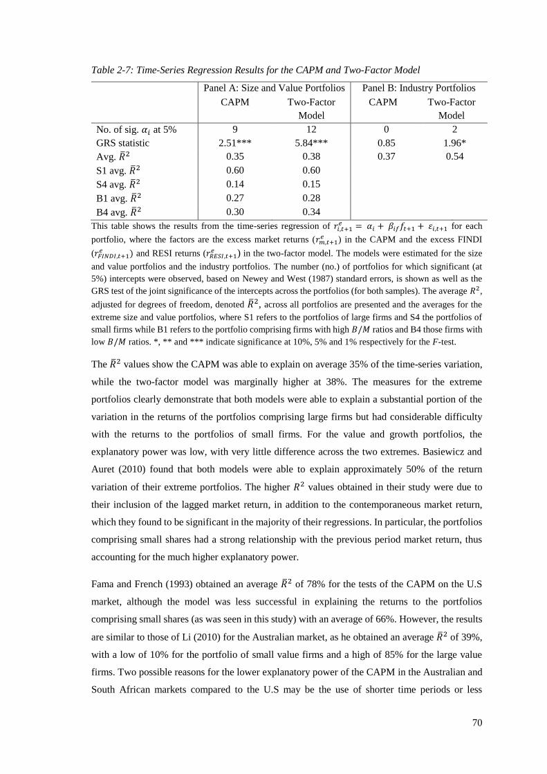
70

Table 2-7: Time-Series Regression Results for the CAPM and Two-Factor Model

Panel A: Size and Value Portfolios Panel B: Industry Portfolios

CAPM Two-Factor

Model

CAPM Two-Factor

Model

No. of sig. 𝛼𝑖 at 5% 9 12 0 2

GRS statistic 2.51*** 5.84*** 0.85 1.96*

Avg. ��2 0.35 0.38 0.37 0.54

S1 avg. ��2 0.60 0.60

S4 avg. ��2 0.14 0.15

B1 avg. ��2 0.27 0.28

B4 avg. ��2 0.30 0.34

This table shows the results from the time-series regression of 𝑟𝑖,𝑡+1𝑒 = 𝛼𝑖 + 𝛽𝑖𝑓𝑓𝑡+1 + 휀𝑖,𝑡+1 for each

portfolio, where the factors are the excess market returns (𝑟𝑚,𝑡+1𝑒 ) in the CAPM and the excess FINDI

(𝑟𝐹𝐼𝑁𝐷𝐼,𝑡+1𝑒 ) and RESI returns (𝑟𝑅𝐸𝑆𝐼,𝑡+1

𝑒 ) in the two-factor model. The models were estimated for the size

and value portfolios and the industry portfolios. The number (no.) of portfolios for which significant (at

5%) intercepts were observed, based on Newey and West (1987) standard errors, is shown as well as the

GRS test of the joint significance of the intercepts across the portfolios (for both samples). The average 𝑅2,

adjusted for degrees of freedom, denoted ��2, across all portfolios are presented and the averages for the

extreme size and value portfolios, where S1 refers to the portfolios of large firms and S4 the portfolios of

small firms while B1 refers to the portfolio comprising firms with high 𝐵/𝑀 ratios and B4 those firms with

low 𝐵/𝑀 ratios. *, ** and *** indicate significance at 10%, 5% and 1% respectively for the F-test.

The ��2 values show the CAPM was able to explain on average 35% of the time-series variation,

while the two-factor model was marginally higher at 38%. The measures for the extreme

portfolios clearly demonstrate that both models were able to explain a substantial portion of the

variation in the returns of the portfolios comprising large firms but had considerable difficulty

with the returns to the portfolios of small firms. For the value and growth portfolios, the

explanatory power was low, with very little difference across the two extremes. Basiewicz and

Auret (2010) found that both models were able to explain approximately 50% of the return

variation of their extreme portfolios. The higher 𝑅2 values obtained in their study were due to

their inclusion of the lagged market return, in addition to the contemporaneous market return,

which they found to be significant in the majority of their regressions. In particular, the portfolios

comprising small shares had a strong relationship with the previous period market return, thus

accounting for the much higher explanatory power.

Fama and French (1993) obtained an average ��2 of 78% for the tests of the CAPM on the U.S

market, although the model was less successful in explaining the returns to the portfolios

comprising small shares (as was seen in this study) with an average of 66%. However, the results

are similar to those of Li (2010) for the Australian market, as he obtained an average ��2 of 39%,

with a low of 10% for the portfolio of small value firms and a high of 85% for the large value

firms. Two possible reasons for the lower explanatory power of the CAPM in the Australian and

South African markets compared to the U.S may be the use of shorter time periods or less

71

diversified portfolios. The first reason, however, can be discarded as Li’s (2010) study utilised a

longer period than in this study starting from 1982. In addition, an analysis of the U.S over the

same period as this research (June 1990 to April 2013) was performed which only yielded a

marginally lower average ��2 of 73%, while that for the portfolios of small shares remained the

same at 66%.27 The use of less-diversified portfolios may account for the lower 𝑅2 values obtained

in the South African studies, as variation in returns may reflect unsystematic factors which the

variation in market returns does not capture. The same is true for some of the size- and value-

sorted portfolios in the Australian sample of Li (2010) (as explained by Brailsford et al., 201228),

with average number of shares as low as seven in his study. However, the fact that the portfolios

with fewer shares in their sample were associated with the portfolios of large firms which yielded

high estimates of ��2 dispels this argument. Moreover, for the South African portfolios, the

explanatory power is still lower than with the U.S tests even for the most diversified portfolios.

Thus, despite considering possible reasons for the lower explanatory power of the CAPM on the

South African market, it appears that the results largely indicate that the model was less successful

in explaining the time-series variation in returns of the size and value portfolios in South Africa

compared to the U.S, but this explanatory power is equivalent to that documented for the

Australian market.

The results from the tests of the intercept for the industry portfolios paint a different picture as for

the CAPM, the joint and individual tests of the intercepts were insignificant, while for the two-

factor model, the joint test was rejected (but only at 10%), but with only two intercepts significant

at 5%. Thus, these results indicate that both models provide a good description of the risk-return

relationship. What is interesting about the intercept estimates, however, is that they are not all

small in magnitude (for example, the telecommunications and health care portfolios had values

of 2.48% and 2.58% respectively), as shown in Table A-2, but rather the standard deviations are

high meaning that the intercepts are estimated with very little precision. These results closely

mirror those of Li (2010) in his test of the CAPM on industry portfolios on the Australian market,

in so far as the majority of the intercepts being insignificant although reasonably large in size.

Accordingly, caution must be exercised in pronouncing the models as a good fit for the industry

sample when the magnitude of the pricing errors remains high. The estimates of explanatory

power are notably higher for the two-factor model than the CAPM, which is driven by high ��2

values for the basic materials, financials and industrials portfolios which are more sensitive to one

of the two factors than the overall market portfolio in the CAPM. This evidence is consistent with

27 Data on the 25 size and value portfolios and the market returns for the U.S to conduct this analysis was

obtained from Kenneth French’s website. 28 Li (2010) employed Brailsford et al.’s (2012) dataset which the latter has formulated prior to their

research being published. The details of this dataset are contained in Brailsford et al. (2012).

72

van Rensburg (2002) in his evaluation of the two models using industry portfolios, which yielded

an average ��2 for the CAPM of 34% and 44% for the two-factor model.

The results of the time-series tests of the CAPM and two-factor model on the two samples thus

provides some conflicting conclusions. The risk premia estimates were insignificant which was

inconsistent with the basic principle of finance that higher risk should be rewarded with higher

returns. However, these estimates did not take into consideration any information from the test

portfolios. The analysis of the time-series regression results revealed that neither model could

explain the size and value anomalies. For the industry portfolios, the two models did have some

success in terms of explanatory power and pricing errors; however, the magnitude of the pricing

errors was still large. As indicated earlier in the chapter, it is imperative to identify a model which

is able to explain all patterns in the share returns, which these two models were not able to do

from a time-series perspective. The extent to which the models were able to explain the cross-

sectional variation in returns is analysed in the following section.

2.6.3 Cross-Sectional Regression Results

The results for the second-stage regressions are shown in Table 2-8. The CAPM and two-factor

model were able to explain 27% and 35% of the variation in returns across the size and value

portfolios respectively, as measured by ��2. The AIC confirmed that the two-factor model

performed better than the CAPM. These ��2 values are quite high compared to those obtained in

equivalent tests of the CAPM in the U.S and Australia of 1% and -0.04% respectively

(Jagannathan & Wang, 1996; Lettau & Ludvigson, 2001b; Li et al., 2011). The industry ��2 values

were markedly higher at 68% and 65% for the CAPM and two-factor models respectively. While

reviewing the explanatory power provides important information regarding the suitability of the

model, this metric is of limited value if the signs and magnitude of the coefficients do not conform

to theory.

The intercepts of the cross-sectional regressions were positive and significant for both

specifications for both sets of portfolios. This contrasts with the theoretical value of zero as there

should be no risk premium when the risk of the asset is zero. This finding is, however, not unique

to the South African market as it has been widely documented since the early seminal studies of

the CAPM, such as Black et al. (1972) and Fama and MacBeth (1973) discussed in section 2.3.3,

to the more recent work of Lettau and Ludvigson (2001b) for example. At face value, this finding

suggests that the risk-free rate proxy used is inappropriate as it understates the return investors

require for holding a riskless asset. This is not surprising given that while individuals can invest

at the 90-day T-bill yield, they cannot borrow at this rate because of their higher risk. Accordingly,

the finding of significant positive intercepts in these regressions supports the argument that the

73

Table 2-8: Cross-Sectional Regression Results for the CAPM and Two-Factor Model


CAPM Two-Factor

Model

CAPM Two-Factor

Model

𝜆0 7.49

(4.81)***

{4.05}***

8.01

(4.85)***

{3.85}***

3.55

(2.87)***

{2.77}***

3.71

(3.80)***

{3.64}***

𝜆𝑚 -6.25

(-3.06)***

{-1.82}*

-2.61

(-1.18)

{-0.66}

𝜆𝐹𝐼𝑁𝐷𝐼 -7.67

(-3.47)***

{-2.05}**

-2.32

(-1.41)

{-0.62}

𝜆𝑅𝐸𝑆𝐼 -4.41

(-1.67)*

{-0.90}

-3.84

(-1.56)

{-0.71}

𝑅2

(��2)

0.32

(0.27)

0.44

(0.35)

0.72

(0.68)

0.74

(0.65)

AIC 1.14 1.07 -1.38 -1.21

Wald statistic 9.38***

{3.31}*

14.74**

{4.99}**

1.39

{0.43}

4.42

{0.88}

RMSE 1.52 1.37 0.55 0.50

Q-statistic 38.91***

{54.90}***

47.90***

{76.00}***

(4.04)

{4.33}

(9.81)

{10.72}

This table reports the coefficients from the Fama and MacBeth (1973) cross-sectional regression ��𝑖,𝑡+1𝑒 =

𝜆0 + 𝜆𝑓′𝛽𝑖𝑓 + 𝜂𝑖, estimated over the period June 1990 to April 2013 across the 16 size and value portfolios

and nine industry portfolios, where 𝛽𝑖𝑓

is a column vector of the sensitivity of the portfolio returns (𝑟𝑖,𝑡+1𝑒 )

to the pricing factors obtained from the time-series regressions. For the CAPM, the factor loading was the

sensitivity to the excess real market returns (𝛽𝑖𝑚) and for the two-factor model, they were the sensitivity to

excess FINDI (𝛽𝑖𝐹𝐼𝑁𝐷𝐼) and RESI returns (𝛽𝑖𝑅𝐸𝑆𝑖). The models were estimated for the size and value

portfolios and the industry portfolios. Beneath each coefficient in round parentheses is the t-statistic

computed using the Fama and MacBeth (1973) standard errors, while the second t-statistic in curly

parentheses was calculated using the Shanken (1992) standard errors. The Wald statistic provides a test of

the joint significance of the coefficients and the Q-statistic tests the joint significance of the model pricing

errors. The values of both of these statistics computed using Shanken’s (1992) standard errors are shown

in curly parentheses. RMSE refers to the root mean squared pricing error across the portfolios. The 𝑅2 is

Jagannathan and Wang’s (1996) cross-sectional measure of explanatory power and ��2 is the value adjusted

for the number of pricing factors. The AIC refers to the Akaike information criteria and was computed

similarly to Jagannathan and Wang’s (1996) 𝑅2. *, ** and *** indicate significance at 10%, 5% and 1%

respectively for the various tests.

return on the minimum-variance zero-beta portfolio may be a more appropriate proxy to capture

the risk-free rate than the T-bill yield. However, the magnitude of the intercepts appears

implausibly high to reconcile this evidence with the use of the zero-beta portfolio. As highlighted

in section 2.3.4, the use of a market portfolio proxy which is not mean-variance efficient may

give rise to a higher measure of the intercept of the SML because of the ‘back-fitting’ nature of

the testing approach. Therefore, this result, rather than highlighting the shortcomings of the risk-

74

free rate proxy may in fact signal the use of an inappropriate market portfolio. Alternatively,

Jagannathan and Wang (1996) argued that this result may indicate that there is important

information missing from the pricing equation.

The CAPM betas for the size and value portfolios from the time-series regressions (which are the

inputs into the cross-sectional regression) are shown in Figure 2-2. The betas for the portfolios of

large firm were, on average, higher than the betas for the portfolios of small firms. This brings

into question the validity of the CAPM, as those portfolios with higher betas should have earned

higher returns, yet as depicted previously, the portfolios comprising the big firms earned less than

the portfolios of small firms. The pattern of betas across the value quintiles was also inconsistent

with the returns documented previously. For the two smaller quintiles, the betas of the value

portfolios were lower than those of the growth portfolios while the opposite was true for the two

larger quintiles. Accordingly, the graphical evidence suggests that beta was not able to adequately

capture the risk-return dynamics.

Figure 2-2: CAPM Betas for the Size and Value Portfolios

This figure plots the market betas for each of the 16 size- and value-sorted portfolios, where the betas were

computed from the time-series regression of 𝑟𝑖,𝑡+1𝑒 = 𝛼𝑖 + 𝛽𝑖𝑚𝑟𝑚,𝑡+1

𝑒 + 휀𝑖,𝑡+1 over the period June 1990

to April 2013 for each of the 16 size and value portfolios, where 𝑟𝑚,𝑡+1𝑒 are the excess real market returns.

S1 refers to the portfolios of large firms and S4 the portfolios of small firms while B1 refers to the portfolios

of firms with high 𝐵/𝑀 ratios and B4 the portfolios of firms with low 𝐵/𝑀 ratios.

These conclusions are confirmed when examining the slope coefficient for the CAPM, shown in

Table 2-8. The market risk premium estimate was negative and significant based on the adjusted

and unadjusted test statistics29. This finding contradicts the basic premise of asset pricing that

29 The measurement approach used for the standard errors had no impact on the conclusions drawn from

the CAPM and two-factor models. This is consistent with the observation of Goyal (2012) for models where

the pricing factor is traded.

75

higher risk should be compensated with higher returns; however, according to Pettengill,

Sundaram, and Mathur (1995) such a finding may not be inconsistent if the realised market returns

were consistently below the risk-free rate during the period studied.30 As documented in Table 2-

6, although insignificant, the market risk premium for the 1990 to 2013 period in South Africa

was positive, with the estimated risk premium found to be significantly different from this value.

Accordingly, not only was the slope of the SML inconsistent with the observed market risk

premium, it also contradicts theory.

As indicated, Fama and French (1992) found evidence of a flat slope for the SML for the U.S,

with Jagannathan and Wang (1996), Lettau and Ludvigson (2001b) and Kullmann (2003) all

confirming this observation. Li et al. (2011) also documented an insignificant positive coefficient

for the market risk premium on the Australian market. Although studies such as Pettengill et al.

(1995) and Elsas, El-Shaer, and Theissen (2003) have countered such findings with evidence

demonstrating a conditional market risk premium which is positive during up-markets and

negative during down-markets, this model still cannot account for the size and value premia

internationally.

The finding of a negative slope for the South African market differs from the early work of

Bradfield et al. (1988), however, it is similar to more recent studies. van Rensburg and Robertson

(2003b) were the first to document a negative relationship between beta and return, with Strugnell

et al. (2011) confirming this relationship, even after numerous methodological adjustments.

Basiewicz (2007) also documented negative risk premia, which were significant in three of the

four specifications. As discussed in section 2.3.6.2, the graphical evidence of Ward and Muller

(2012) revealed that this negative relationship has become flatter since 2004, as per the

international studies. To assess the veracity of their conclusion, the CAPM regression tests were

repeated only using data from July 2004 to April 2013. These cross-sectional tests (results not

shown) confirmed the conclusion of Ward and Muller (2012) as the coefficient was insignificant.

Consequently, the evidence suggests that the beta-return relationship on the JSE has changed over

time with the market now more closely resembling the dynamics observed for the U.S and other

international markets. Charteris (2014), on a set of industry-sorted portfolios, also confirmed that

accounting for market upswings and downswings, as per Pettengill et al. (1995), was not able to

salvage the CAPM on the JSE, as she still found a significant negative coefficient for the up-

market periods. The similarity in findings between this study and recent work in this area on the

30 Pettengill et al. (1995) argued that although the CAPM is an expectational model, tests thereof use

realised returns and thus should account for the possibility that the market risk premium may be negative,

which the standard equations tested do not.

76

JSE suggests that the use of quarterly rather than monthly data, with the consequent reduction in

the number of time-series observations, did not bias the results obtained.

For the two-factor model, the resources premium entered with a negative sign but was

insignificant; a finding consistent with the time-series risk premium for this index over the sample

period. However, the same was not true for the premium on the financials and industrials index,

which was significant and negative for the size- and value-sorted portfolios in contrast to the

actual positive risk premium. Thus, irrespective of whether the market was measured in aggregate

or in its component parts the same patterns emerged. Although Basiewicz (2007) did not provide

details from his regressions, the summary information provided indicated that for the equivalent

model on his sample, at least one of the slope coefficients was significant and had a negative

coefficient. Thus, the results from this study appear to largely be consistent with his findings.

Accordingly, despite the marginally higher explanatory power of the two-factor model compared

to the CAPM, the specification does not provide an improved description of the cross-section of

share returns on the JSE based on the coefficient estimates.

The CAPM and two-factor regressions on the industry portfolios yielded insignificant slope

coefficients, as shown in Table 2-8. However, this is inconsistent with the relatively high

explanatory power observed for these portfolios. As documented previously, the variation across

the industry portfolio returns was relatively low, which yields a high cross-sectional 𝑅2 due to

the manner in which this statistic is computed (as per equation 2.52) even though the factors are

not priced. Thus, the analysis of the coefficients revealed that neither of these models was able to

price the industry portfolios; with the CAPM result consistent with Li’s (2010) findings for

Australia. The minimal variation across the industry portfolios makes them difficult assets to price

as pointed out by Li et al. (2011).

With a single-factor model, like the CAPM, the Wald test provides limited additional insight, as

it simply confirms the conclusions drawn from the test of significance of the slope coefficient.

With the two-factor model, the Wald statistics signal that the model was able to explain a

significant portion of the cross-sectional variation in the size- and value-sorted portfolios but not

the industry-sorted portfolios, with the former principally emanating from the financials and

industrials index rather than the resources index. However, caution must be exercised in

interpreting this value, as the slope coefficient has little economic meaning because of the

negative sign.

The final analysis of these two models was the pricing errors, with the RMSE and the Q-statistics

also shown in Table 2-8. For the size and value portfolios the RMSE was lower for the two-factor

model compared to the CAPM but the Q-statistics showed that the null hypothesis that the pricing

77

errors were jointly equal to zero could be rejected at 5% for both specifications.31 These results

are consistent with the conclusions drawn from the other measures of the model suitability and

those of Basiewicz (2007), who documented similar chi-squared statistics for both models. The

international studies cited previously, such as Lettau and Ludvigson (2001b) for the U.S and Li

et al. (2011) for Australia, obtained similar findings for the CAPM, although the magnitude of the

errors (and related statistics) were smaller for South Africa as a consequence of the better fit of

the model because of the significant (albeit negative) priced factor. The pricing errors for each of

the size and value portfolios for the CAPM, displayed in the figure below, demonstrate that the

CAPM had difficulty explaining the returns to the extreme portfolios; a result consistent with the

U.S evidence depicted by Lettau and Ludvigson (2001b). Although there were a few exceptions,

the small firm portfolios and those portfolios of firms with high 𝐵/𝑀 ratios plotted below the line

(with the opposite true for the big and growth firm portfolios) indicating that their realised returns

exceeded those predicted by the model.

Figure 2-3: Pricing Errors from the CAPM for the Size and Value Portfolios

This figure plots the pricing errors from the cross-sectional regression ��𝑖,𝑡+1𝑒 = 𝜆0 + 𝜆𝑚𝛽𝑖𝑚 + 𝜂𝑖 over the

period June 1990 to April 2013 across the 16 size and value portfolios, where 𝛽𝑖𝑚 measures the sensitivity

of the portfolio returns to the excess real market returns. S1 refers to the portfolios of large firms and S4

the portfolios of small firms while B1 refers to the portfolios comprising firms with high 𝐵/𝑀 ratios and

B4 the portfolios of those firms with low 𝐵/𝑀 ratios.

The Q-statistics from both models for the industry-sorted portfolios indicated that the null

hypothesis that the errors were equal to zero could not be rejected. This finding, alongside the ��2,

31 As shown in Table 2-8, it is possible for a model to have a lower RMSE than another model but a higher

Q-statistic because of the difference in the way the RMSE is calculated compared to the statistics. Similar

patterns were evident in the results of Lettau and Ludvigson (2001b), Santos and Veronesi (2006) and Li

et al. (2011).

78

provides support for the models, which is inconsistent when evaluated against the signs and

significance of the pricing factors. Thus, the low variation in returns across the industry portfolios

also gives rise to minor cross-sectional pricing errors. This highlights the importance of

examining several measures of the model veracity rather than relying on a single metric which

may provide an inaccurate conclusion. In light of the evidence presented, neither the CAPM nor

the two-factor models were able to explain the industry-sorted portfolio returns, as with the size-

and value-sorted portfolios.

2.6.4 GMM Regression Results

The GMM regression results for the two models are shown in Table 2-9. The coefficient from the

linear SDF for the CAPM is significant for the size and value portfolios. However, the significant

value for the J-test confirms that this factor alone was not sufficient to explain returns as the

model yielded substantial pricing errors. Moreover, consistent with the previous results from the

cross-sectional Fama and MacBeth (1973) regressions, the transformed market risk premium for

the CAPM was significant but negative. For the two-factor model, the J-test also resulted in the

rejection of the null hypothesis that the pricing errors were equal to zero. The results from the

SDF indicated that both the RESI and FINDI helped in pricing securities, with the transformed

risk premia confirming that these factors were both priced, albeit again with the wrong sign. This

differs slightly from the cross-sectional results where only the FINDI was found to be priced.

For the industry-sorted portfolios, the J-tests suggest that the pricing kernels of both the CAPM

and two-factor model were able to explain returns across these portfolios. However, as was found

when evaluating the results for these portfolios in the preceding section, none of the factors were

priced or, in the case of the two-factor model, helped to price the portfolios given the presence of

other factors. This result thus again points to the shortcomings of the industry portfolios due to

the lack of variation. Overall, the results from the GMM analysis largely confirm that neither the

CAPM nor the two-factor model were able to explain portfolio returns.

2.7 CONCLUSION

This chapter provided a theoretical and empirical review of the CAPM; a model which represents

the cornerstone of asset pricing. Although the CAPM has been evaluated previously in South

Africa, this model was tested on the JSE, in conjunction with van Rensburg’s (2002) two-factor

model which accounts for segmentation on the market. This was done both as a basis of

comparison against which models tested in the remaining chapters of this study could be

compared but also to provide a thorough examination of the cross-sectional implications of the

models, which had only briefly been considered in the unpublished work of Basiewicz (2007).

79

The results showed that neither of the two models were able to explain the returns on the size and

value or the industry portfolios, and, if anything, the CAPM performed worse on the JSE than

internationally, as a significant negative market risk premium was identified. Similar findings

were documented for the two-factor model. The evidence was consistent across the various

methods employed. The results of the analysis of the CAPM thus invoke the thoughts of Ross

(1993:13) that “The CAPM is a wonderful theory. It is also useless in a practical way.”

In light of the poor performance of these asset pricing models it was critical to explore alternative

asset pricing models so as to be able to better understand the risk-return relationship. In the

following chapter some of the extensions to the CAPM which are also seen as portfolio-based

models are reviewed, and thereafter the alternative macroeconomic-based view of asset pricing is

introduced.

Table 2-9: GMM Regression Results for the CAPM and Two-Factor Model


CAPM Two-Factor Model CAPM Two-Factor Model

𝑏𝑚 0.08***

(6.87)

0.01

(1.04)

𝑏𝐹𝐼𝑁𝐷𝐼 0.05***

(2.89)

0.01

(0.48)

𝑏𝑅𝐸𝑆𝐼 0.03**

(2.62)

0.01

(0.71)

J-statistic 66.65*** 68.61*** 7.71 7.32

𝜆𝑚 -7.65***

(-6.95)

-1.26

(1.20)

𝜆𝐹𝐼𝑁𝐷𝐼 -5.52***

(-2.92)

-0.66

(1.38)

𝜆𝑅𝐸𝑆𝐼 -5.78***

(-2.65)

-1.27

(1.77)

This table shows the coefficients from Hansen’s (1982) optimal two-stage GMM estimation of the SDF

𝑚𝑡+1 = 𝛼 + 𝑏′𝑓𝑡+1, where 𝑚𝑡+1 is the SDF, 𝑓𝑡+1 is a column vector of the pricing factors and 𝛼 was

normalised to one. For the CAPM, 𝑓𝑡+1 included the excess market returns (𝑟𝑚,𝑡+1𝑒 ) and for the two-factor

model the factors were the excess FINDI (𝑟𝐹𝐼𝑁𝐷𝐼,𝑡+1𝑒 ) and RESI returns (𝑟𝑅𝐸𝑆𝐼,𝑡+1

𝑒 ). The models were

estimated for the size and value portfolios and the industry portfolios. The transformed risk premia (𝜆) are

presented in the bottom half of the table and were computed from the SDF coefficients as 𝜆 = −𝑣𝑎𝑟(𝑓)𝑏,

where 𝑣𝑎𝑟(𝑓) is the variance of the pricing factor. Beneath both the 𝑏’s and 𝜆’s the t-statistics are displayed

in round parentheses, with the standard errors of the 𝑏’s based on the Newey and West (1987) method,

while those for the transformed 𝜆’s were computed using the delta method. Hansen’s (1982) J-statistic for

the test of the pricing errors is also shown. *, ** and *** indicate significance at 10%, 5% and 1%


80

Chapter 3 : PORTFOLIO AND MACROECONOMIC ASSET

PRICING MODELS

3.1 INTRODUCTION

Given the limiting assumptions of the CAPM and its poor performance in empirical tests, various

extensions to the portfolio-based asset pricing model have been developed. These models are

viewed as multifactor asset pricing models as they expand the measurement of risk beyond the

CAPM’s beta. Two principle motivations underpin the models that have been developed – either

empirical or theoretical. The theoretically motivated models, such as the conditional CAPM,

intertemporal CAPM and APT, seek to relax one or more of the restrictive assumptions of the

CAPM which do not reflect the real-world complexities of investing. In contrast, Fama and

French’s (1993) three-factor model, was driven by the asset pricing anomalies, as identified in the

previous chapter, such that they added ad hoc pricing factors to the CAPM on the basis that they

must proxy for unobservable risk.

A contending school of thought downplays these portfolio-based models, both the theoretical and

empirical models, on the basis that even if these models perform well, they do not actually explain

how share prices are determined as they simply show how share returns are correlated with a set

of factors (portfolios) that by derivation should perfectly fit all asset returns if the mean-variance

efficient portfolio is used (Cochrane, 2008a, pp. 242-243). Instead, the approach of this group

entails trying to understand how macroeconomic factors drive asset prices. The consumption

CAPM represents one of the cornerstones of this research.

Although the portfolio-based models do not necessarily provide information about the underlying

determinants of share returns, many of these models do still provide valuable insight about the

return-generating process. Most notable in this regard are the intertemporal and conditional

models which incorporate time-variation in returns and risk as opposed to the static one-period

CAPM. As the conditional model provides more information about this time-variation component

than the intertemporal model and has played a prominent role in further developments in asset

pricing, this model is tested on the JSE. Fama and French (1993)’s three-factor model has become

the empirical standard for asset pricing, given its substantial success. Thus this model is also

evaluated so as to provide a basis against which other models tested in chapters 4 and 5 could be

compared, as well to understand its cross-sectional explanatory power which has not previously

been examined on the JSE. Finally, the consumption CAPM is tested on the South African market

so as to ascertain the ability of this macroeconomic factor model to explain the size and value

anomalies. Most of the international studies on this model have focused on developed markets

81

and thus it is of value to ascertain whether this potentially critical macroeconomic variable

represents a universal determinant of returns.

The remainder of the chapter is laid out as follows: models which incorporate time-variation are

reviewed, followed by an analysis of other multifactor pricing models. An introduction to

macroeconomic factor models is provided, with the derivation of the consumption CAPM and its

empirical performance discussed. Thereafter, the chosen models are tested on the JSE and the

results compared both to the international literature and the performance of the CAPM and two-

factor model tested in chapter 2.

3.2 TIME-VARYING ASSET PRICING MODELS

Studies have shown that share returns are predictable over time. If this predictability of returns

reflects that the amount of risk and an investor’s willingness to bear risk vary over time, especially

over business horizons, then the parameters in the SDF will depend on investor’s expectations of

future returns (Lettau & Ludvigson, 2001b). However, as indicated in the previous chapter, the

CAPM assumes that the parameters in the SDF are constant over time. Thus the finding of

predictability of share returns has potentially important implications for explaining differences in

returns across assets (Cochrane, 2008b, pp. 244) and as such, the empirical evidence and relevant

theoretical issues pertaining to time-series predictability are reviewed in this section. Thereafter,

the two principle asset pricing models that allow for time-variation - the intertemporal CAPM and

conditional CAPM - are discussed.

3.2.1 Time-Series Predictability of Returns

3.2.1.1 Empirical Evidence of Predictability

As defined in section 2.3.1, an efficient market is one in which share prices fully and immediately

reflect all available information implying that future share returns should not be predictable.

Numerous studies over the past 25 years have examined whether publicly available information

and information contained in past prices can be used to predict share returns and earn abnormal

returns; contrary to the EMH. The regression used for determining the ability of a variable to

predict nominal excess returns is

𝑟𝑚,𝑡+1𝑒 = 𝜅′𝑍𝑡 + 𝑣1,𝑡+1, (3.1)

where 𝑍𝑡 is a vector of lagged predictor variables and 𝜅′ represents a vector of coefficients (Lettau

& Ludvigson 2010, p. 633). Several studies (such as Fama & French, 1989; Lettau & Ludvigson,

2010) have also tested equation 3.1 using real returns, with similar results obtained. A myriad of

82

financial variables and ratios have been examined for their forecasting power, with some of the

most successful detailed below.

𝐷/𝑃 and 𝐸/𝑃 ratios (or their inverses, 𝑃/𝐷 and 𝑃/𝐸). Early studies by Fama and French

(1988a) and Hodrick (1992) found these ratios to have substantial predictive power for

excess returns. However, Lamont (1998) demonstrated that 𝐷/𝑃 was more successful

than 𝐸/𝑃 because earnings exhibit greater variability (that is unrelated to share returns)

than dividends leading to noisier predictions of share returns. More recently, contrasting

results have been documented, with Ang and Bekaert (2007) finding that 𝐷/𝑃 was only

able to predict share returns in the presence of the short-term interest rate, while Lettau

and Ludvigson (2010) found no forecasting power for this ratio.

Short-term interest rates. Fama and Schwert (1977), Hodrick (1992) and Lamont (1998)

showed that the short-term interest rate, usually measured as the relative T-bill yield (the

difference between the monthly rate and its twelve-month moving average), was able to

predict returns, especially at short-horizons. Lettau and Ludvigson (2001a), Ang and

Bekaert (2007) and Lettau and Ludvigson (2010) confirmed this conclusion.

Default and term spreads. The default spread measures the difference between the yields

on high-grade (e.g. AAA-rated) and lower-grade (e.g. BAA-rated) corporate bonds, while

the term spread captures the difference between the yields on long-term and short-term

Treasury bonds. Keim and Stambaugh (1986) found that these two spreads could predict

future returns. Fama and French (1989) and Lettau and Ludvigson (2010) combined these

two measures with 𝐷/𝑃 (and the short-term interest rate in the latter study) and found

that although they could explain a proportion of the time-series variation in returns, their

forecasting power was not as significant as 𝐷/𝑃 (and the short-term interest rate).

Equation 3.1 examines the forecasting power of variables at one-period ahead, with the research

predominantly focusing on one-month, one-quarter or one-year ahead as daily and weekly returns

appear not to be predictable (Cochrane, 2005, pp. 390). Additionally, most studies also consider

the ability of the variables to predict excess market returns over longer horizons, as follows

𝑟𝑚,𝑡+𝐻,𝐻𝑒 = 𝜅𝐻′𝑧𝑡 + 휀1,𝑡+𝐻,𝐻, (3.2)

where 𝑟𝑚,𝑡+𝐻,𝐻𝑒 is the 𝐻-quarter continuously compounded excess return equal to 𝑟𝑚,𝑡+1 −

𝑟𝐹,𝑡+1 + ⋯ + 𝑟𝑚,𝑡+𝐻 − 𝑟𝐹,𝑡+𝐻 (Lettau & Ludvigson, 2010, p. 635). One of the principle reasons

for examining relationships multiple periods ahead is because the relationships are believed to be

clearer because they eliminate noise (Valkanov, 2003). Moreover, studies have also found that

83

some variables contain more information about long-run rather than short-run future returns. For

example, Fama and French (1989) found that major movements in 𝐷/𝑃 were related to long-term

trends that covered several business cycles, whereas the term spread was more closely related to

short-term business cycles. Rasmussen (2006) obtained similar evidence.

The finding of share return predictability using publicly available information therefore suggests

that markets are not efficient (or at the most only weak-form efficient as information such as term

spreads and the 𝐷/𝑃 ratio is publicly available). Several scholars have attributed these findings

to statistical errors in the methodology while others contend that such predictability arises from

the rational response of investors to time-varying investment opportunities. These arguments are

briefly reviewed in the following sections.

3.2.1.2 Methodological Limitations as an Explanation for Predictability

Several studies (including Hodrick, 1992; Nelson & Kim, 1993; Stambaugh, 1999; Valkanov,

2003; Ang & Bekaert, 2007) have shown that the finding of long-run predictability may be more

of a matter of statistics than economics arising from the use of overlapping returns in the long-

run regressions. For example, the value of a two-period ahead return in period 𝑡 + 232 would be

computed as the sum of the return in period 𝑡 + 2 and 𝑡 + 1, while that in period 𝑡 + 3 would be

the sum of the return in periods 𝑡 + 3 and 𝑡 + 2. Thus, the observations in period 𝑡 + 3 and 𝑡 + 2

both include the return in period 𝑡 + 2 leading to autocorrelation in the residuals. For a three-

period ahead return, there would be two overlapping returns and thus more generally, for an 𝐻-

period ahead return, there would be 𝐻 − 1 overlapping returns (Vila-Wetherwilt & Wells, 2004).

Serial correlation in the residuals may lead to incorrect inferences regarding predictability because

the standard errors are not efficient.

Valkanov (2003) also demonstrated that even though the original return series is stationary, the

rolling summation leads to the series behaving asymptotically like a non-stationary process. This

means that the t-statistics and regression 𝑅2 values will not converge to the t-distribution and their

population values respectively. Accordingly, the long-run regressions may indicate the existence

of a relationship even when there is not one (Valkanov, 2003). These effects are more pronounced

when the forecast horizon is long compared to the sample size. However, the finding of

predictability for many variables remains even after making adjustments for this overlapping data

(see for example Valkanov, 2003; Rasmussen, 2006; Lettau & Ludvigson, 2010).

32 The observation at 𝑡 + 1 would effectively be “lost” for a two-period ahead return as there would only

be one period (𝑡 + 1) to include.

84

The predictor variables have also been subjected to criticism, especially 𝐷/𝑃 and 𝐸/𝑃, as these

ratios are highly persistent (and thus close to non-stationary) and thus predictability effectively

accumulates over long horizons leading to high explanatory power for the regressions (Hodrick,

1992). In fact, even the one-period ahead forecasts can be considered biased, as they tend to inherit

the near unit root properties of the forecasting variable leading to inflated test statistics, which

may thus suggest predictive ability even if there is none (Boudoukh, Richardson, & Whitelaw,

2008). Once adjustments are made for this persistence in the forecasting variable, the predictive

power declines substantially and in some cases appears to be non-existent (see for example

Hodrick, 1992; Goetzmann & Jorion, 1993; Nelson & Kim, 1993; Stambaugh, 1999); although

other authors contend that predictability remains even after adjusting for the persistence

(Lewellen, 2004; Campbell & Yogo, 2006).

In addition to these shortcomings, the form of these tests are criticised as they assess the

forecasting power of variables based on in-sample (data for the full-period is used to predict

values that are already included in the dataset) rather than out-of-sample data and therefore the

relationships are likely to be biased upwards. Goyal and Welch (2007) documented that these

‘successful’ forecasting variables in the in-sample tests have limited out-of-sample predictability;

however, Eliasz (2005), Inoue and Kilian (2005) and Rapach and Wohar (2006) presented

contrasting evidence as they found that these variables do have out-of-sample predictive power.

Moreover, Inoue and Kilian (2005) found that in-sample tests have more power asymptotically

than out-of-sample tests, with Goyal and Welch (2007) conceding that tests of predictability

should not be based solely on out-of-sample tests.

3.2.1.3 Reconciling Time-Series Predictability with Theory

Although the evidence of time-series predictability is weaker following the statistical adjustments

described, sufficient evidence of predictability remains which, as specified previously, suggests

that markets are not efficient. However, Campbell and Shiller (1989) derived a theoretical

paradigm (extended by Campbell, 1991; Cochrane, 1992) showing that predictability is not

necessarily inconsistent with the idea of efficiency as predictability can arise because of time-

variation in risk and returns, which is captured by variation in the rate at which investors discount

future income from risky assets. To see this, it is necessary to briefly consider the traditional

pricing equation and the expanded version which allows for time-variation in returns.

The intrinsic value of a share is usually determined by Gordon’s (1962) dividend growth model

(Drake & Fabozzi, 2012), which proposes that the current price of a share is equal to the

discounted value of all expected future dividends. In this specification, the required rate of return,

which is determined by the risk of the security, is assumed to be constant. According to the model,

85

any variation in the share price over time will thus be caused by variation in the dividend growth

rate (Campbell et al., 1997, pp. 256). However, empirical work on volatility in share returns by

LeRoy and Porter (1981) and Shiller (1981) demonstrated that volatility in share returns was too

high to be accounted for only by variation in future dividend growth discounted at a constant rate.

In conjunction with this evidence and the growing body of research indicating predictability in

returns, Campbell and Shiller (1989) devised a specification for the 𝑃/𝐷 ratio, consistent with

market efficiency, which allows for time-variation in the dividend growth rate and returns. The

starting point for their model is the compound share return 𝑟𝑖,𝑡 = 𝑙𝑛 (𝑃𝑡+𝐷𝑡

𝑃𝑡−1) ∗ 100 (equation 2.40).

By taking a first-order Taylor series expansion of this return around the point 𝑃

𝐷= 𝑒𝑝−𝑑, applying

a transversality condition (that rules out rational bubbles in asset prices) and taking expectations

yields

𝑝𝑡 − 𝑑𝑡 ≈ 𝜔 + 𝐸𝑡 ∑ 𝜌𝑖𝑗(Δ𝑑𝑡+𝑗

∞𝑗=1 − 𝑟𝑖,𝑡+𝑗), (3.3)

where lower case letters refer to the natural logs of the variables, 𝑝𝑡 − 𝑑𝑡 is the natural log of the

𝑃/𝐷 ratio at time 𝑡, Δ𝑑𝑡+𝑗 measures growth in dividends, 𝜌𝑖 = (1 + 𝑒𝑝−𝑑 )−1 and 𝑝 − 𝑑 is the

average 𝑃/𝐷 ratio (Campbell & Shiller, 1989, p. 201).33 Campbell and Shiller (1989) termed this

model the dynamic Gordon growth model. Equation 3.3 shows that when share prices are high

relative to dividends (𝑃/𝐷 is high) investors either anticipate low future returns from securities

or high growth rates in dividends (Cochrane, 2005, pp. 397).

To determine whether it is dividend growth or share returns that follow 𝑃/𝐷, Campbell and Shiller

(1989) computed the variance of the ratio. Cochrane (2008b, pp. 1544) showed that this can easily

be obtained by multiplying both sides of equation 3.3 by (𝑝𝑡 − 𝑑𝑡) − 𝐸(𝑝𝑡+1 − 𝑑𝑡+1) and taking

unconditional expectations as it yields

𝐸[(𝑝𝑡 − 𝑑𝑡)(𝑝𝑡 − 𝑑𝑡)] ≈ 𝐸[(𝑝𝑡 − 𝑑𝑡) ∗ ∑ 𝜌𝑖𝑗(Δ𝑑𝑡+𝑗

∞𝑗=1 − 𝑟𝑖,𝑡+𝑗).

The left-hand side of this equation represents the variance of 𝑃/𝐷, while the right-hand side can

be simplified resulting in the following

𝑣𝑎𝑟(𝑝𝑡 − 𝑑𝑡) ≈ 𝑐𝑜𝑣((𝑝𝑡 − 𝑑𝑡), ∑ 𝜌𝑖𝑗Δ𝑑𝑡+𝑗

∞𝑗=1 ) − 𝑐𝑜𝑣((𝑝𝑡 − 𝑑𝑡) ∑ 𝜌𝑖

𝑗∞𝑗=1 𝑟𝑖,𝑡+𝑗) (3.4)

(Cochrane, 2008b, p. 1544). From this equation it can be seen that any variation in the 𝑃/𝐷 ratio

arises either because of the covariance of the ratio with growth in dividends or returns. Stated

33 The constant is excluded from the equation for the purposes of simplicity as it has no effect on the

analysis.

86

differently, the 𝑃/𝐷 ratio can only vary if it forecasts growth in dividends and/or returns j periods

ahead. If dividend growth and returns cannot be forecasted, then their expected value must be the

same at every point in time such that 𝑃/𝐷 will be constant. Campbell (1991), Cochrane (1992)

and, more recently, Cochrane (2008b) tested this relationship and found that nearly all of the

variation in 𝑃/𝐷 was attributable to variation in returns rather than the dividend growth rate.

Accordingly, this result solidifies the evidence that 𝑃/𝐷 forecasts returns in a framework which

is still consistent with an efficient market.

Another way of looking at equation 3.3 is that if dividend growth and stock returns are both

stationary on the right-hand side, then the 𝑃/𝐷 ratio on the left-hand side must be stationary

implying that dividends and prices are cointegrated (MacDonald & Power, 1995). This means

that dividends and prices cannot wander too far from each other so any deviations in the long-run

relationship must be corrected for in the future. Such corrections will occur either through a

movement in the dividend growth rate or share return or both; thus giving rise to predictability

that is still consistent with the EMH (Lettau & Ludvigson, 2010, pp. 624).

While initial studies on the forecasting ability of 𝑃/𝐷 documented supporting evidence, as

indicated, more recent studies have found contending results especially after accounting for

statistical shortcomings in the earlier work. Cochrane (2008b), in an influential paper on the

subject, contended that the null hypothesis specified in these tests of no share return predictability

is incorrect, as it ignores the implications of equation 3.3 leading to erroneous inferences. That is,

he maintained that the null hypothesis should capture the fact that if excess returns are not

predictable then dividends must be predictable. The results of Cochrane’s (2008b) tests led to the

rejection of this adjusted null hypothesis, with the principle driving force behind this rejection

being the absence of predictability in dividend growth rather than the existence of strong evidence

of return predictability. Cochrane (2008b) thus concluded that there was no “shred of evidence”

that dividends could be forecasted and as such share returns must be predictable.

The fact that returns are forecastable from 𝐷/𝑃, which arises because of variations in returns and

not dividend growth, suggests that returns should also be predictable from past returns. At long

horizons, Fama and French (1988b) and Lettau and Ludvigson (2001a) confirmed this

relationship with the negative sign consistent with the idea of mean reversion. However, the more

recent studies of Cochrane (2005, p. 415), Rasmussen (2006) and Lettau and Ludvigson (2010)

found no evidence of univariate predictability. This evidence therefore suggests that while returns

are forecastable from 𝐷/𝑃, they are not forecastable from their own past values. This is not a

contradiction, but simply reflects the differing forms information can take (consistent with the

distinction outlined in the EMH).

87

3.2.1.4 Time-Series Predictability and Business Cycles

Given this framework that suggest that time-variation in returns is not inconsistent with the EMH,

such patterns in returns over time must be driven by rational investor behaviour, with studies such

as Fama and French (1989), Ang, Piazzesi, and Wei (2004), Cochrane (2008a) and Lettau and

Ludvigson (2001a; 2010) linking this to a response by investors to investment opportunities which

vary with business cycles and risk aversion. Fama and French (1989) explained that expected

returns vary over the business cycle, with expected returns high during bad times when investors

are less willing to hold risks, while the opposite is true for good periods. When expected returns

rise, prices fall which should thus lead the market to require higher expected returns in the

following period, leading to predictability. For example, certain risks may be higher during

market troughs than peaks, with these risks captured by 𝑃/𝐷 or the default spread for example.

Moreover, variation in returns across business cycles could also be related to consumption

patterns. Assuming investors prefer to smooth consumption over time, when income is high

relative to wealth, investors want to smooth consumption into the future by saving more; higher

savings should lead to lower expected returns ceteris parabus. The converse is true when income

is temporarily low as investors will want to save less driving expected returns up. These ideas

have been further extended in the habit formation models, such as that of Campbell and Cochrane

(1999). They argued that investors slowly develop habits for levels of consumption and

accordingly, their current utility is a function of how much they usually consume. During bad

times, when consumption drops below its habit level, the risk aversion of investors increases and

they thus demand a higher premium while the opposite is true when the economy is in a good

state. Therefore, risk aversion varies with business conditions. Other models linking idiosyncratic

labour income risks have also been postulated to explain rational time-variation in returns (see

Constantinidis & Duffie, 1996). Fama and French (1989) also asserted that variation in capital

investment opportunities may generate variation in expected returns. For example, poor prospects

for future real activity (and thus investments) near business peaks may help to explain low

expected returns around peaks. Likewise, good prospects for future activity and investment after

troughs may contribute to high expected returns around troughs.

The common factor behind these ideas is that returns are linked to the macroeconomy, with high

expected returns associated with a low 𝑃/𝐷 or 𝑃/𝐸 (or a high 𝐷/𝑃 and 𝐸/𝑃), an upward sloping

yield curve, high default spreads or low interest rates; all of which are associated with

macroeconomic downturns (Ang & Bekaert, 2007; Cochrane, 2008b). The view that predictability

may be associated with variation across business cycles has driven much of the more recent work

in this area as given the link between returns and business cycles, it is argued that macroeconomic

variables are likely to reflect changing patterns and therefore play an important role in forecasting

88

future share returns (Lettau & Ludvigson, 2001a). The predictive power of several

macroeconomic variables has also been assessed directly with success for metrics such as the

investment/capital ratio (Cochrane, 1991), the cyclical component of industrial production

(Daniel & Torous, 1995; Hodrick & Zhang, 2001) and the output gap (the difference between

actual and potential output that can be produced by an economy at full capacity) (Cooper &

Priestley, 2009). Further evidence thereof is presented in chapters 4 and 5.

3.2.1.5 Time-Series Predictability in South Africa

In South Africa, very little work had been conducted on the time-series predictability of share

returns until a series of papers by Gupta and Modise (2012a, 2012b, 2013). They examined the

ability of valuation ratios and financial and economic variables to forecast share returns, with

various adjustments to account for statistical shortcomings. They found that the T-bill rate and

term spread had reasonable predictive power over short horizons (Gupta & Modise, 2012b).

However, 𝐷/𝑃 and 𝐸/𝑃 had little success in forecasting returns (Gupta & Modise, 2012a). For

the macroeconomic factors, money supply and interest rates were identified to have some

forecasting ability (Gupta & Modise, 2013).

3.2.2 The Intertemporal CAPM

The evidence that share returns are predictable over time is consistent with the description of

equilibrium in the intertemporal CAPM that investors’ willingness to bear risk varies over

business horizons. This, however, contends with the simple CAPM, as was recognised early in

the development of the literature. Merton (1973), building on the ideas of Fama (1970b), argued

that investors are concerned about more than expected returns and variance (as in the CAPM), as

they also take cognisance of their long-term wealth in their decision-making. Merton (1973)

assumed that investors seek to maximise consumption over the course of their lifespan based on

a concave von Neumann-Morgenstern utility function for consumption.34 This concern for

lifetime utility means that investors attempt to anticipate and hedge against unfavourable

movements in their investment opportunity set in the future. Such hedging can effectively be seen

as protection of their consumption levels or future payoffs from the original investment. Investors

make predictions about the future using state variables – variables that are able to predict future

34Although the intertemporal CAPM is derived from assumptions regarding consumption rather than mean-

variance utility, which distinguishes the model from the CAPM, consumption does not explicitly enter as a

pricing factor as is the case with the consumption CAPM (which is discussed in section 3.4.1). Rather, it

gives rise to the multi-period framework and the role of hedging portfolios. The intertemporal CAPM can

thus be viewed as an extension to the CAPM (see Brennan, Wang, & Xia, 2004; Cochrane, 2005, 2008a).

However, other scholars (such as Fama, 1991; Campbell et al., 1997) view the model as a precursor to the

consumption CAPM.

89

market premia – which are then incorporated into their risk-return expectations. An investor will

thus hold three types of portfolios in equilibrium – the market portfolio, the risk-free asset and 𝑧

hedging portfolios (one for each state variable). Fama (1996) termed the optimal portfolios in this

framework multifactor efficient, as they have the largest possible expected returns, given the

variance of their returns and the covariance with the state variables.

For an individual security, the intertemporal CAPM implies the following pricing relationship

𝐸𝑡(𝑟𝑖𝑒) = [

−𝐽𝑤𝑤𝑊

𝐽𝑤] 𝐸𝑡(𝑐𝑜𝑣(𝑟𝑖, 𝑟𝑚)) + ∑ [

−𝐽𝑤𝑧

𝐽𝑤] 𝐸𝑡(𝑐𝑜𝑣(𝑟𝑖, Δ𝑧))𝑍

𝑧=1 , (3.5)

where 𝑊𝑡+1 denotes wealth and 𝑧𝑡+1 is the vector of state variables that describe wealth (Merton,

1973, p. 878). 𝐸𝑡(𝑐𝑜𝑣(𝑟𝑖, 𝑟𝑚)) and 𝐸𝑡(𝑐𝑜𝑣(𝑟𝑖, Δ𝑧)) are the expected covariance of the security

returns with the market and with the state variable respectively. 𝐽(𝑊𝑡+1, 𝑧𝑡+1) is the indirect

utility function of wealth and 𝐽𝑤 and 𝐽𝑤𝑤 are the first and second derivatives thereof. [−𝐽𝑤𝑤𝑊

𝐽𝑤] is

the measure of risk aversion or price of risk and should be positive if the investor is risk averse

(Merton, 1973, p. 878).

Campbell (1996) showed that this model can be written in discrete time as follows

𝐸(𝑟𝑖,𝑡+1𝑒 ) = 𝛾𝑖 + 𝛾𝑖𝑚𝑐𝑜𝑣(𝑟𝑖,𝑡+1, 𝑟𝑚,𝑡+1) + 𝛾𝑖𝑧′𝑐𝑜𝑣(𝑟𝑖,𝑡+1, Δ𝑧𝑡+1), (3.6)

where 𝛾𝑖𝑚 is the risk premium and is known as the parameter of relative risk aversion (as it

captures the willingness of investors to bear risk) and 𝛾𝑖𝑘 denotes the covariance risk price

associated with the state variable (Maio & Santa-Clara, 2012, p. 589). Equation 3.6 shows that

the first source of risk in the intertemporal CAPM is the co-movement between the security

returns and the market, as per the CAPM. Assuming investors are risk-averse, an asset that moves

positively with the market does not provide a hedge against current wealth as it pays out when

returns are already high. Investors would thus only be willing to hold such an asset if it offers a

risk premium, as captured by the parameter of relative risk aversion (Cochrane, 2005, pp. 166).

According to Mehra and Prescott (1985), this parameter of relative risk aversion should lie

between one and ten, with tests of the intertemporal CAPM examining whether this condition is

met.

The hedging needs of investors gives rise to the second source of risk in the model, which is

captured by the covariance of the share returns with each hedging portfolio. If the state variable

forecasts positive excess market returns and the intertemporal risk premium is positive, it means

that the security moves in the same direction as the future market risk premium. Accordingly, a

risk-averse investor will demand a positive intertemporal risk premium (𝛾𝑖𝑧) to hold such a

security, as it does not provide a hedge against changes in wealth (Maio & Santa-Clara, 2012).

90

The intertemporal CAPM thus places a constraint on the sign of 𝛾𝑖𝑧 that is informed by the

relationship between the state variable and the future risk premium (Maio & Santa-Clara, 2012).

If the price of the intertemporal risk is zero, then the intertemporal CAPM reduces to the CAPM.

By standardising each covariance measures in 3.6 by the variance of the factor, the intertemporal

model can be written as a linear factor model in the expected return-beta framework as

𝐸(��𝑖,𝑡+1𝑒 ) = 𝜆0 + 𝜆𝑖𝑚𝛽𝑖,𝑚 + 𝜆𝑖Δ𝑧′β𝑖,Δ𝑧, (3.7)

where 𝛾𝑖𝑚 = 𝜆𝑖𝑚 ∗ 𝑣𝑎𝑟(𝑟𝑚) and 𝛾𝑖𝑧 = 𝜆𝑖𝑧 ∗ 𝑣𝑎𝑟(𝑟Δ𝑧) for each state variable (Maio & Santa-

Clara, 2012).

As is evident, the intertemporal CAPM, like the CAPM, was derived in the portfolio theory

framework. However, it has also been mapped into the SDF setup (see Cochrane, 2005, p. 167;

Campbell, Giglio, Polk, & Turley, 2012). Drawing on Dybvig and Ingersoll’s (1982) proof that a

linear factor pricing model is equivalent to a linear SDF (as shown in section 2.2.2.2), the

specification of the intertemporal CAPM in 3.7 implies the standard SDF, as per equation 2.22,

𝑚𝑡+1 = 𝑎 + 𝑏′𝑓𝑡+1, (3.8)

But where 𝑓𝑡 is a matrix of the 𝑧 state variables (which includes the market portfolio) (Cochrane,

2005, p. 165).

The intertemporal CAPM does not explicitly identify the state variables, and thus many studies

simply add ad hoc pricing factors and attribute them to the intertemporal CAPM; leading Fama

(1991) to term this process ‘fishing for factors’. However, there is a clear set of criteria by which

to evaluate candidate state variables; albeit that this is not regularly implemented in tests

(Campbell, 1996; Maio & Santa-Clara, 2012). That is, these state variables must be able to

forecast future returns and the sign of the risk premium must be identical to that in the predictive

regression. Accordingly, variables which have been found to be able to predict share returns (such

as the 𝐷/𝑃 ratio and term spread) have been used to represent the state variables.35 In light of the

fact that these variables are able to predict share returns because of their close correlation with

the business cycle, the intertemporal CAPM thus provides a link between share prices and the

macroeconomy, although it is still a portfolio-based model.

Despite the strong theoretical foundations of the intertemporal CAPM, the tests thereof have

produced mixed results. Brennan et al. (2004), for example, found that the model could explain

35 Brennan et al. (2004) advocated a synthetic approach to constructing the state variable; however, this

approach is not widely used.

91

patterns in returns for the size- and value-sorted portfolios but not industry-sorted portfolios;

while Cederburg (2011) documented that although the model could explain some of the size and

value anomalies, it could not capture all the variation in returns. Most recently, Maio and Santa-

Clara (2012), in a comprehensive test of the ability of the intertemporal CAPM to explain returns

on the 25 size and 𝐵/𝑀-sorted portfolios using several state variables, found that in almost all the

models, the parameter of relative risk aversion was negative and the signs of the risk prices for

the hedging portfolios did not match those from the predictive regressions.

Although the intertemporal CAPM has not achieved substantial success empirically, the multi-

period framework provides a strong theoretical foundation that has played an important role in

the development of the asset pricing paradigm, especially in the consumption CAPM. Moreover,

as is detailed in the following section, despite some substantial differences to the conditional

CAPM, the intertemporal and conditional models yield very similar pricing equations.

3.2.3 The Conditional CAPM

Numerous studies have documented that betas vary over time (see for example Bollerslev, Engle,

& Wooldridge, 1988; Chan & Chen, 1988; Ferson & Harvey, 1991; 1993; Ang & Chan, 2007).

Jagannathan and Wang (1996) argued that this variation is both rational and consistent with

theory. For example, distressed and/ or highly levered firms are more likely to face financial

distress during recessions, with any changes in the market value of a firm’s debt leading to

changes in the overall risk of the firm. This variation in risk may assist in explaining the variation

in returns over time, as documented in section 3.2.1; however, neither the CAPM nor

intertemporal CAPM consider this possibility. The conditional CAPM, in contrast, considers the

flow of information over time that may affect beta, the risk premium as well as the relationship

between these two variables (Levy, 2012, pp. 175). Although this model is frequently attributed

to the work of Jagannathan and Wang (1996), earlier studies by Ferson and Harvey (1991, 1993)

laid the foundations for the model. Extending the work of Jagannathan and Wang (1996),

Cochrane (1996, 2005) and Lettau and Ludvigson (2001b) showed how this conditional pricing

relation can also be expressed as an SDF.

3.2.3.1 The Conditional CAPM of Jagannathan and Wang (1996)

Jagannathan and Wang (1996:8) defined the conditional CAPM as follows

𝐸(��𝑖,𝑡+1𝑒 |𝐼𝑡) = 𝛾0𝑡 + 𝛾1,𝑡𝛽𝑖𝑚,𝑡, (3.9)

where 𝐼𝑡 is the information the investor has at time t, which is a subset of all information Ω (i.e

𝐼𝑡 ⊂ Ω). The conditional beta in equation 3.9 is computed as

92

𝛽𝑖𝑚,𝑡 =𝑐𝑜𝑣(𝑟𝑖,𝑡+1

𝑒 , 𝑟𝑚,𝑡+1𝑒

|𝐼𝑡)

𝑣𝑎𝑟(𝑟𝑚,𝑡+1𝑒 |𝐼𝑡)

. (3.10)

Equations 3.9 and 3.10 appear identical to the equivalent CAPM formula specified in chapter 2;

the difference, however, is that in this case, beta is measured at each point in time, as denoted by

the time subscript, based only on the available information. Taking unconditional expectations of

equation 3.9 results in

𝐸(��𝑖,𝑡+1𝑒 ) = 𝛾0 + 𝛾1��𝑖𝑚 + 𝑐𝑜𝑣(𝛾1,𝑡 , 𝛽𝑖𝑚,𝑡) (3.11)

where 𝛾0 = 𝐸[𝛾0,𝑡], 𝛾1 = 𝐸[𝛾1,𝑡] and ��𝑖𝑚 = 𝐸[��𝑖𝑚,𝑡] (Jagannathan & Wang, 1996, p. 8). In this

model, 𝛾1 captures the expected market risk premium and ��𝑖𝑚 is the expected market beta. The

last term in 3.11 measures the covariance between the conditional market beta and risk premium

such that firms which are more closely correlated with the conditional market risk premium will

yield a higher return. For example, the beta of a distressed and/or highly levered firm is likely to

be higher during a recession than for a firm which is affected less by an economic downturn. The

conditional market risk premium will also be high during a recession to compensate investors for

the higher risk during bad economic times and hence the risk premium and the measure of risk

will be correlated. This term would thus account for time variation in expected returns, which is

consistent with the evidence presented in section 3.2.1.1.

Jagannathan and Wang (1996, p. 9) defined the sensitivity of the conditional beta to the market

risk premium, denoted 𝜗𝑖, as follows

𝜗𝑖 = 𝑐𝑜𝑣(𝛾1,𝑡, 𝛽𝑖𝑚,𝑡)/𝑣𝑎𝑟(𝛾1,𝑡), (3.12)

which can be used to compute the residual beta (𝜂𝑖,𝑡)

𝜂𝑖,𝑡 = 𝛽𝑖𝑚,𝑡 − ��𝑚𝑖 − 𝜗𝑖(𝛾1,𝑡 − 𝛾1). (3.13)

The first two terms in 3.13 capture the difference between the conditional and unconditional betas,

with the third term adjusting this difference for the deviation of the risk premium from its

unconditional value (Krause, 2001, p. 52). This equation implies that 𝐸(𝜂𝑖,𝑡) = 0 and that 𝜂𝑖,𝑡 is

uncorrelated with the conditional market risk premium (𝑐𝑜𝑣(𝜂𝑖,𝑡, 𝛾1,𝑡) = 0) (see Krause, 2001, p.

53 for the proof thereof). Rearranging 3.13 the conditional beta for security 𝑖 can be written as

𝛽𝑖𝑚,𝑡 = ��𝑖𝑚 + 𝜗𝑖(𝛾1,𝑡 − 𝛾1) + 𝜂𝑖,𝑡 (3.14)

(Jagannathan & Wang, 1996, p. 9). This equation demonstrates that the time-varying beta

comprises of a constant component (the expected beta, ��𝑖𝑚), a random component that is perfectly

93

correlated with the market risk premium (𝜗𝑖), and a component which is uncorrelated with the

market (𝜂𝑖,𝑡) and should be zero (Jagannathan & Wang, 1996, p. 9). Substituting 3.14 into 3.11

𝐸(��𝑖,𝑡+1𝑒 ) = 𝛾0 + 𝛾1��𝑖𝑚 + 𝜗𝑖𝑣𝑎𝑟(𝛾1,𝑡), (3.15)

which shows that the unconditional expected return on a security is a function of the expected

beta and the sensitivity of the beta to the conditional market risk premium (Jagannathan & Wang,

1996, p. 10). The beta premium sensitivity captures the instability of the asset’s beta over the

business cycle, with securities with greater sensitivity to the market risk premium earning higher

returns. As is evident from 3.15, the residual beta has no impact on unconditional returns.

This derivation thus shows that the single-factor conditional CAPM of 3.9 yields a two-factor

unconditional pricing model. The problem is that the right-hand side variables in equation 3.15 –

the expected beta and beta premium – cannot be directly estimated. However, Jagannathan and

Wang (1996) demonstrated that the expected return can be written as a linear function of two

unconditional betas36, with the first being the traditional market beta and the second a premium

beta, which captures beta instability risk. This can be seen as follows

𝐸(��𝑖,𝑡+1𝑒 ) = 𝜆0 + 𝜆𝑚𝛽𝑖𝑚 + 𝜆𝛾𝛽𝑖

𝛾, (3.16)

where

𝛽𝑖𝛾

=𝑐𝑜𝑣(𝑟𝑖,𝑡+1

𝑒 ,𝛾1,𝑡)

𝑣𝑎𝑟(𝛾1,𝑡) (3.17)

(Jagannathan & Wang, 1996, p. 10). Shares which are more highly correlated with the business

cycle (as captured by the expected market risk premium) will thus have a high 𝛽𝑖𝛾 leading to a

higher risk premium. This makes sense as investors will have to be induced to hold securities

which pay off when the expected market risk premium is already high. The conditional market

risk premium (𝛾1𝑡) needed to compute this parameter is also not directly observable and thus an

instrument or set of instruments, denoted by the vector 𝑧𝑡, that can forecast the future market risk

premium are usually used. In this case, the conditional betas are denoted 𝛽𝑖𝑧, as they capture the

sensitivity of the security returns to the future market risk premium.

As highlighted in section 3.2.1.4, returns may vary across business cycles for a variety of rational

reasons, such as variation in investment opportunities, higher risk during market troughs than

peaks, and investors attempting to smooth consumption patterns over time (the latter is discussed

in more detail in section 3.4.1). Irrespective of the cause of this variation, 𝛽𝑖𝑧 should capture the

36 The mathematics of this process are complex and the details thereof are contained in appendix A of

Jagannathan and Wang’s (1996) study.

94

sensitivity of the share returns to variation across business cycles through the conditioning

variable. Thus, although Jagannathan and Wang (1996) set out to capture variation in beta over

time, their ability to implement a practical model effectively yielded a pricing equation which

captures variation in returns that is not directly related to the market beta. However, the model

proposed by Cochrane (1996) and further expanded by Lettau and Ludvigson (2001b), discussed

in the next section in the SDF framework, does account for variation in the market beta.

3.2.3.2 The Conditional CAPM in the SDF Framework

As highlighted in section 2.2.2.1, the standard SDF (𝑝𝑖,𝑡 = 𝐸𝑡[𝑚𝑡+1𝑥𝑖,𝑡+1]) is assumed to hold

at each point in time meaning that it must hold unconditionally giving rise to the SDF of 𝐸(𝑝𝑖,𝑡) =

𝐸[𝑚𝑡+1𝑥𝑖,𝑡+1]. However, assuming investors have access to all information may not be an

accurate reflection of reality. This unconditional SDF, however, can be adjusted to account for

the information that investors do have access to as follows

𝑝𝑖,𝑡 = 𝐸[𝑚𝑡+1𝑥𝑖,𝑡+1| 𝐼𝑡] if 𝑝𝑖,𝑡 ∈ 𝐼𝑡 (3.18)

(Cochrane, 2005, p. 133). Cochrane (1996, p. 582) proposed implementing this conditional SDF

by scaling the payoffs by a set of instruments 𝑧𝑡 observable at time t (𝑧𝑡 ∈ 𝐼𝑡)

𝑝𝑖,𝑡𝑧𝑡 = 𝐸𝑡[𝑚𝑡+1𝑥𝑖,𝑡+1𝑧𝑡], (3.19)

and then taking the unconditional expectations yields

𝐸(𝑧𝑡𝑃𝑖,𝑡) = 𝐸[𝑚𝑡+1𝑋𝑖,𝑡+1𝑧𝑡]. (3.20)

This shows that expanding the pricing equation to consider conditioning information can be

achieved simply by the use of variables which forecast future market conditions (Campbell, 2000,

pp. 1526). The same scaling would apply to the SDF expressed in terms of excess returns rather

than prices as 0 = 𝐸[𝑚𝑡+1𝑟𝑖,𝑡+1𝑒 𝑧𝑡] (Cochrane, 1996, p. 582).

In the unconditional models the parameters in 𝑚𝑡+1, 𝛼 and 𝑏, are assumed to be constant.

However, these parameters may vary over time as the vector of instruments (zt) varies across

different information sets. Accordingly, 𝛼 and 𝑏 can be modelled as a linear37 function of zt over

time as 𝛼𝑡 = 𝛼0 + 𝛼1zt and 𝑏𝑡 = 𝑏0 + 𝑏1zt (Campbell, 2000, pp. 1526).38 Thus, to test a model

37 Considering a linear specification is sufficient, as a non-linear function can be expressed simply as an

additional instrument in the same framework (Cochrane, 1996, pp. 583). 38 Cochrane (1996, pp. 583) only scaled the 𝑏 parameter in his study. However, this ‘full’ model which

allows for the time-varying slope and intercept in the pricing kernel was proposed by both Lettau and

Ludvigson (2001b) and Cochrane (2005) in 1999 in unpublished versions of their work (Campbell, 2000,

pp. 1526).

95

in which the factors are only expected to price securities conditionally, equation 2.22 for 𝑚

(𝑚𝑡+1 = 𝛼 + 𝑏′𝑓𝑡+1) can be rewritten as

𝑚𝑡+1 = 𝛼0 + 𝛼1zt + 𝑏0′𝑓𝑡+1 + 𝑏1′𝑓𝑡+1zt (3.21)

(Lettau & Ludvigson, 2001b, p. 1246). For the CAPM, this model can be written as

𝑚𝑡+1 = 𝛼0 + 𝛼1zt + 𝑏0𝑟𝑚,𝑡+1𝑒 + 𝑏1zt𝑟𝑚,𝑡+1

𝑒 . (3.22)

This specification thus allows for the intercept and the market price of risk to vary across business

cycles (Hodrick & Zhang, 2001). As with the traditional CAPM and intertemporal CAPM, this

SDF can be expressed as a linear model in the expected return-beta framework as

𝐸(��𝑖,𝑡+1𝑒 ) = 𝜆0 + 𝜆𝑧𝛽𝑖𝑧 + 𝜆𝑚𝛽𝑖𝑚 + 𝜆𝑚𝑧𝛽𝑖𝑚𝑧 (3.23)

(Lettau & Ludvigson, 2001b, p. 1258; Cochrane, 2005, p. 144). Thus, the conditional model with

time-varying coefficients is expressed as a three-factor model with fixed coefficients. The first

source of risk in this model captures how returns vary with the future market risk premium (𝛽𝑖𝑧)

and is thus identical to the factor put forward by Jagannathan and Wang (1996) in their model.

This term is often referred to as the time-varying intercept because of how it is derived in the SDF

framework (Lettau & Ludvigson, 2001b). The traditional market beta represents the second

source of risk, which also mirrors Jagannathan and Wang’s (1996) model. The distinction between

this model and that of Jagannathan and Wang (1996) lies in the third source of risk (𝛽𝑖𝑚𝑧), which

measures the interaction between the security and the scaled market returns. This term captures

how the market beta varies over business cycles and effectively measures the time-variation in

risk that Jagannathan and Wang (1996) sought to incorporate into the pricing equation (Campbell,

2000, p. 1526). This term is often referred to as the time-varying slope coefficient because of how

it is derived in the SDF framework (Lettau & Ludvigson, 2001b).

The key requirement for the conditioning variables is that they must be able to predict share

returns (Cochrane, 1996) and thus they can be seen to be similar to the state variables of the

intertemporal CAPM. Hence, the variables identified in the time-series predictability literature

are employed for this purpose. The use of the same variables to predict future market risk premia

in the intertemporal and conditional models highlights the similarity between these two

specifications. However, in the former, the risk factors are changes in the variables whereas in

the latter, the lags of these variables are used (Campbell, 1996, pp. 312). The underlying

principles of the models also differ which can be seen in the interpretation of the risk premia on

the instruments for the future market risk premium. For the intertemporal CAPM, the co-

movement of returns with the future market risk premium captures the hedging component of

96

investor behaviour whereas with the conditional CAPM, this coefficient captures the risk

premium associated with the time-varying component of risk. The other notable difference is that

the conditional CAPM (from the SDF framework) includes an additional risk measure describing

the interaction between the security returns and the scaled market returns.

3.2.3.3 Empirical Tests of the Conditional CAPM

Jagannathan and Wang (1996) tested their model (equation 3.16) using the default spread as the

conditioning variable. They found that the conditional CAPM was able to explain 30% of the

variation in share returns compared to only 1% for the CAPM for beta and size-sorted portfolios,

although the pricing errors were still significant. Although the market risk premium was

insignificant, the coefficient on the time-varying intercept was positive and significant

demonstrating that shares which moved more closely with the business cycle were compensated

with greater returns. This coefficient remained significant when size was included as an additional

factor in the pricing equation, while size was only marginally significant. Therefore, there was

some evidence to suggest that some of the size anomaly may reflect time-variation not accounted

for in the CAPM. Kullmann (2003) also tested this model on the U.S market but using the T-bill

yield to predict the future market risk premium. She obtained very similar results to Jagannathan

and Wang (1996) in terms of explanatory power on the size and beta-sorted portfolios (𝑅2 of

25%) and the conditional beta was priced while the market beta was not. The conditional risk

premium had a negative coefficient demonstrating that those shares which were highly negatively

correlated with the interest rate earned a higher return. This mirrors the finding from the

forecasting literature that interest rates are inversely related to the state of business conditions.

The consistency in results across these two studies thus shows that the conditional CAPM was

not sensitive to the choice of conditioning variable.

Hodrick and Zhang (2001) conducted further tests but utilised the three-factor specification of

Lettau and Ludvigson (2001b) for the conditional CAPM, with the cyclical component of

industrial production as the scaling variable. They also examined whether the model could explain

both the size and value anomalies as opposed to only the former in the previous two studies

reviewed. Hodrick and Zhang (2001) found that the conditional market risk premium was not

significant suggesting that market risk did not vary over business cycles. However, the conditional

risk premium and the market risk premium were positive and significant indicating that portfolios

which moved more closely with the state of the business cycle and the market generated a higher

risk premium. The model was able to account for some of the anomalous returns to value and

small firms and thus despite the significant pricing errors, Hodrick and Zhang (2001) still

concluded that the inclusion of industrial production provided important information that was

missing from the CAPM.

97

In time-series tests of the model, Petkova and Zhang (2005) found that the risk of value shares

moved positively with the expected market risk premium, captured by several variables (the 𝐷/𝑃

ratio, short-term interest rate and default and term spreads), whereas the betas of the growth shares

moved in the opposite direction to the expected market risk premium. This behaviour of value

and growth shares can explain why the former require a risk premium to induce investors to hold

these shares because they pay off when expected returns are already high, whereas growth shares

do not have to offer such a premium as they payoff when expected returns are low. Despite some

success in explaining the value premium, Petkova and Zhang (2005) acknowledged that allowing

for variation in returns across business cycles was not sufficient to capture all of the premium.

Lewellen and Nagel (2006) argued that the cross-sectional tests of the conditional CAPM, such

as those of Jagannathan and Wang (1996) and Hodrick and Zhang (2001), do not provide a

sufficient test of the model as they ignore the restrictions on slope terms that are implied by the

theory. That is, that the coefficient on the market beta should be equal to the market risk premium

and the slope coefficient on the conditional market beta should be equal to the covariance between

the market risk premium and the conditioning variable. Given the difficulty associated with

imposing these restrictions, Lewellen and Nagel (2006), similarly to Petkova and Zhang (2005),

conducted time-series tests of the conditional CAPM. They derived the time-series intercept

(pricing error) of the unconditional model as the product of the correlation between beta and the

expected market risk premium and the standard deviations of the two components. By assuming

values for these three components, Lewellen and Nagel (2006) calibrated estimates for the

intercept. Under the most extreme conditions (highest standard deviations and a correlation of

one), the maximum possible pricing error was only 0.35%, with most values less than 0.2%. These

estimates thus provided a benchmark for comparison purposes, as if the conditional CAPM holds,

the values of the intercept obtained in tests of the model should not exceed these values.

To avoid using a scaling variable, Lewellen and Nagel (2006) estimated the CAPM over very

short windows using high frequency data, with the pricing errors then averaged to obtain a single

estimate. The pricing errors for the value-sorted portfolios were positive and significant and much

larger than any of the calibrated values; thereby confirming that the conditional CAPM was not

able to explain the value anomaly. In contrast, the values of the intercept were insignificant for

the size-sorted portfolios, but this was due to the absence of the size premium in the sample as

opposed to the model being able to explain the returns on these portfolios. An analysis using the

conventional instruments for the market risk premium yielded identical results. Accordingly, the

findings of Lewellen and Nagel (2006) confirmed those of Petkova and Zhang (2005), that while

betas do vary with the conditional market risk premium it was not substantial enough to account

for the anomalies.

98

Ang and Kristensen (2012) supported the methodological approach adopted by Lewellen and

Nagel (2006) in testing the conditional CAPM but argued that their tests were limited because

they did not allow the time-variation in the betas to directly influence the time-varying intercept

estimates. Ang and Kristensen (2012) thus derived more encompassing tests that enabled both the

individual and joint significance of the pricing errors across the portfolios to be examined. Despite

the improved testing measure, their results were consistent with the previously mentioned studies

that the conditional model was not able to explain the value anomaly.

3.2.3.4 Conclusions Regarding the Conditional CAPM

Although the conditional CAPM has achieved only limited success in explaining the size and

value anomalies, the model has featured prominently in more recent asset pricing research

because of the patterns that have been identified in the data that returns and betas vary over time.

Consequently, as will be highlighted in chapters 4 and 5, research has focused on trying to identify

a more suitable variable to predict business cycles rather than the more conventional instruments.

3.3 OTHER MULTIFACTOR PRICING MODELS

As was seen in the review of the intertemporal and conditional models, the allowance for the time-

variation in risk and return resulted in multifactor models compared to the single-factor of the

CAPM. Several other multifactor models have been derived, however, the notable difference to

the intertemporal and conditional models, is that the use of several pricing factors in these models

is motivated by identifying a more comprehensive measure of risk than the CAPM beta rather

than due to time-variation. Two of the most prominent of these models – the APT and Fama and

French (1993) three-factor model - are reviewed in this section.

3.3.1 The APT

The APT, of Ross (1976), proposes that the expected return on a share is a linear function of a set

of f-factors as follows

𝐸(𝑟𝑖,𝑡+1𝑒 ) = 𝛼𝑖 + ∑ 𝛽𝑖𝑓𝑓𝑡+1

𝐹𝑓=1 , (3.24)

where 𝑓𝑡+1 are the risk factors that impact the returns of security i and 𝛽𝑖𝑓 is the factor loading

which measures the sensitivity of security i’s return to the factor (Cochrane, 2005, p. 175). Given

the link between the expected return-beta pricing equation and the SDF, the APT pricing kernel

can be specified as

𝑚𝑡+1 = 𝑎 + 𝑏′𝑓𝑡+1 (3.25)

99

(Cochrane, 2005, p. 176). This pricing equation is identical to the intertemporal CAPM of

equation 3.8; yet, the models are derived under different conditions and the interpretation of the

coefficients are also distinct.

In contrast to the previous models examined, APT makes no assumptions about investor

behaviour, with the equilibrium pricing equation resulting from arbitrage under the law of one

price (Roll & Ross, 1980). This was one of the reasons for the original popularity of the model

compared to the CAPM or intertemporal CAPM, which rely on restrictive assumptions about

investor behaviour. However, the view that APT does not necessitate any economic restrictions

is an oversimplification as the law of one price can only be extended so far in order to derive the

pricing equation after which approximations are required (Dybvig & Ross, 1985; Shanken 1985).

As with the CAPM, the APT assumes that investors hold diversified portfolios of securities such

that only the covariance of the security with the risk factor is of importance in determining the

return. However, the problem with this approach is that the systematic risk must affect the average

investor; that is, if the risk affects some investors but not others, then it will not be priced. For

example, if an event makes investor A worse off and investor B better off, then the former will

purchase securities that do better when the event happens while the latter will sell them. They

transfer the risk of the event so that the price of the security (and therefore the return) is unaffected

such that the factor will not be correlated with the covariance of returns. Thus, there may be

common risk factors that are not rewarded (if the two groups are approximately equal in size),

even though the returns of a large number of securities move with the factor (Cochrane, 2005, pp.

172).

Two distinct approaches have been adopted in the literature to determine the identity of the risk

factors. The first, pioneered by Roll and Ross (1980), Reinganum (1981), Lehmann and Modest

(1988) and Connor and Korajczyk (1988), relied on the use of factor analysis to identify common,

significant factors, in security returns. These statistically-derived specifications, however, have

not only performed poorly in empirical tests, but this approach has also been criticised because

no meaning can be assigned to the risk factors (Chen & Jordan, 1993). The studies of van

Rensburg and Slaney (1997) and van Rensburg (2002) on the JSE, which identified the distinct

resources and financials/ industrials sectors, made use of this factor analysis approach. As

mentioned in chapter 2, van Rensburg’s (2002) two-factor model can be seen as an APT model.

But the model was not classified as such in this study, but rather as an alternative way of

measuring the market portfolio, which is consistent with van Rensburg (2002).

The alternative method of determining the factors entails testing a set of pre-specified factors,

usually macroeconomic variables, as they are likely to affect all shares. The seminal study of

Chen et al. (1986) showed that inflation, the term structure of interest rates, the yield spread and

100

industrial production were important explanatory influences on returns. Similar international

studies, such as Hamao (1988) on the Japanese market, and Poon and Taylor (1991) and Antoniou,

Garrett, and Priestley (1998) on the U.K market, have shown that these factors are not universal.

For example, industrial production was insignificant in the Japanese market and none of the

factors were priced in the U.K based on Poon and Taylor’s (1991) results, although Antoniou et

al. (1998) found inflation to be significant when examining a longer sample period and also found

money supply to be priced. Moreover, despite the role of such factors in pricing security returns,

there is very little evidence to suggest that the APT can explain the size and value anomalies

(Chen et al., 1986). In South Africa, variables such as interest rates as well as factors unique to

the resource-based South African economy (such as the Rand gold price and the production of

gold) have been found to be important APT factors (see van Rensburg, 1996, 1997, 1998, 1999,

2000). Kan and Zhang (1999) showed that the usual t-test of significance is flawed, if the true

model is not known ex ante as is the case with APT (the same is also true of the intertemporal

CAPM). Accordingly, these authors argued that the findings of the importance of macroeconomic

factors in pricing securities must be interpreted with some caution.

This evidence highlights two important shortcomings of this macroeconomic modelling approach.

Firstly, the selection of the variables is ad hoc, and thus can be used as a justification for

introducing any factor into the pricing equation. Although the intertemporal CAPM framework

has been viewed as ‘a fishing licence’, the pricing factors in this model must not only be justified

theoretically as state variables but in so doing, must be able to forecast future returns. The same

is not true for APT factors, where the sole requirement for the inclusion of a pricing factor is that

the factor can describe the covariance matrix of returns. Secondly, although a set of factors may

be able to explain returns in one period, this does not imply that it will be able to do so in another,

as was true for inflation in the U.K studies. This arises because the variance of share returns is

not constant over time (Fama & French, 2006). Accordingly, this attests to the value of the

intertemporal CAPM relative to the APT where, as indicated, the intertemporal CAPM factors

must be able to forecast the conditional distribution of returns.

In light of the theoretical and empirical shortcomings of the APT, its popularity has waned, as

scholars favour the theoretical strengths of models such as the conditional CAPM. The fact that

the model receives no attention in Cochrane’s (2008a) review of developments in the asset pricing

literature is a testament to this. More recently, Campbell’s (2014) review of empirical asset

pricing (arising from the awarding of the 2013 Nobel prize in economics to Eugene Fama, Lars

Peter Hansen and Robert Shiller) also makes no mention of the APT. The principle reason for the

lack of use of the APT is that researchers focusing on the link between the macroeconomy and

asset pricing are not principally concerned about whether a particular macroeconomic factor

affects aggregate returns (as per the APT) but rather whether the factor affects investor’s

101

behaviour in their demand for securities. Accordingly, the APT model is not considered directly

in this study.

3.3.2 The Fama and French (1993) Three-Factor Model

Given the vast evidence of the size and value anomalies, Fama and French (1993) recognised the

shortcomings of the CAPM and instead proposed a three-factor asset pricing model. This model

included two additional portfolios (other than the market return) so as to capture the sensitivity of

an asset’s returns to size and value on the basis that these characteristics must proxy for common,

non-diversifiable risk factors in returns. The size factor is computed as the return on a portfolio

long small shares and short big shares (small minus big, denoted SMB) and the value factor is

computed as the returns on a portfolio long firms with high 𝐵/𝑀 shares and short firms with low

𝐵/𝑀 (high minus low, denoted HML) (Fama & French, 1993, pp. 9). The model is as follows

𝐸(��𝑖,𝑡+1𝑒 ) = 𝜆0 + 𝜆𝑚𝛽𝑖𝑚 + 𝜆𝑆𝑀𝐵𝛽𝑖𝑆𝑀𝐵 + 𝜆𝐻𝑀𝐿𝛽𝑖𝐻𝑀𝐿, (3.26)

where 𝛽𝑖𝑆𝑀𝐵 and 𝛽𝑖𝐻𝑀𝐿 measure the sensitivity of the portfolio returns to SMB and HML

respectively. Consistent with the link between a linear factor model and the SDF, 3.26 implies a

pricing kernel for the model of

𝑚𝑡+1 = 𝑎 + 𝑏𝑚𝑟𝑚,𝑡𝑒 + 𝑏𝑆𝑀𝐵𝑆𝑀𝐵𝑡+1 + 𝑏𝐻𝑀𝐿𝐻𝑀𝐿𝑡+1. (3.27)

As briefly mentioned in section 2.3.4, in time-series tests of the CAPM, Fama and French (1993)

found that the model was able to explain a large proportion of the variation in the 25 size and

𝐵/𝑀 portfolios over time (with ��2 values between 61% and 92%). However, the three-factor

model explained more variation with ��2 values in excess of 90% for 21 of the 25 portfolios, with

the many significant HML and SMB betas indicating that these additional two factors captured

variation in the share returns that was not captured by the market. Moreover, the intercepts from

the time-series regression of the three-factor model were only significant for three of the portfolios

compared to the ten for the CAPM and the pattern of higher pricing errors for the small and value

firm portfolios was no longer evident (Fama & French, 1993). Although the joint test of the

intercepts was rejected for the Fama and French (1993) model, as with the CAPM, in a follow-up

study on the U.S market, the GRS test for the three-factor model could not be rejected (Fama &

French, 1996), suggesting that the results from the initial study could be attributed to the inclusion

of seven bond portfolios in addition to the 25 size- and value-sorted portfolios when the joint test

was conducted. Davis et al. (2000) confirmed that the empirical success of the three-factor model

was robust to the inclusion of more firms and a longer sample period. Fama and French’s (1996)

results also showed that the three-factor model was able to explain the returns of portfolios sorted

based on 𝐸/𝑃, cash flow yield and five-year sales rank, adjusted for size, although it was not able

102

to explain returns to momentum-sorted portfolios.39 In addition, both studies found that the three-

factor model still has difficulty in explaining returns to the portfolios of the smallest firms.

Jagannathan and Wang (1996) conducted a cross-sectional test of the three-factor model in their

U.S study and found that the model was able to explain 55% of the variation across size and beta-

sorted portfolios. Lettau and Ludvigson (2001b) found that the three-factor model was able to

explain close to 80% of the variation across the 25 size and value portfolios, compared to 1% for

the CAPM. They identified only small pricing discrepancies for the small value and growth, and

large value and growth portfolios; however, this mispricing on these extreme portfolios did give

rise to the rejection of the joint test that the cross-sectional pricing errors were equal to zero.

Studies of the explanatory power of the three-factor model in international markets have been

hard to conduct because of the lack of reliable data over a long time-series, with many studies

only considering one additional factor. For example, Fama and French (1998) only evaluated the

market returns and HML in their sample of thirteen countries from Asia, Australasia and Europe,

while Heston, Rouwenhorst, and Wessels (1999) included only size and the market risk premium

for their twelve European countries. Despite this limitation both of these studies found that the

inclusion of the additional risk factor yielded substantially higher explanatory power than using

the market returns only. However, the results of Heston et al. (1999) revealed that the regression

intercepts were jointly significant, in contrast to Fama and French (1998), possibly suggesting a

more important role for the value rather than the size factor. Heston et al. (1999) also showed, in

aggregate and for each of the European countries, that the market and size betas were important

determinants of the cross-section of share returns. Bagella et al. (2000) conducted a test of the

three-factor model on the London stock exchange and found that although the model provided a

substantial increase in R2 relative to the CAPM in explaining the time-series returns, the pricing

errors were jointly significant. Brailsford et al. (2012) undertook a comprehensive examination

of the three-factor model on the Australian market including both time-series and cross-sectional

tests. From the former, the regression intercepts were found to be insignificant for all but one of

the portfolios, with the joint test confirming this conclusion. In the cross-sectional tests all three

factors were priced, with an ��2 of 72% providing a notable improvement on the CAPM of 42%.

39 Carhart (1997) included an additional risk factor to the three-factor model to account for momentum,

known as WML (winners minus losers), which he found could account for the strong negative returns for

the previous year’s losers and the strong positive returns for the previous year’s winners. This model

however, is predominantly used as a means of measuring the performance of fund managers, through

Carhart’s alpha, rather than for asset pricing because it is hard to reconcile the momentum factor with

unobservable risk that is not captured by beta, as is the case for the size and value factors (as highlighted in

chapter 2). Moreover, as discussed in section 1.3.1, the existence of the momentum anomaly is often

attributed to the irrational behaviour of investors rather than the use of an inappropriate asset pricing model.

103

On the South African market, Basiewicz and Auret (2010), discussed in chapter 2, also considered

the suitability of the three-factor model. Based on the 𝑅2 figures, the three-factor model was able

to explain a greater proportion of the returns of 12 size and value portfolios over time than the

CAPM and van Rensburg’s (2002) two-factor model, and the figures were comparable to

international studies, ranging between 52% and 89%. The joint GRS test of the regression

intercepts showed that the three-factor model did not have significant pricing errors. However,

further analysis revealed that while the three-factor model was largely able to explain the value

effect, it did not adequately account for the size effect. Nonetheless, Basiewicz and Auret (2010)

contended that the Fama and French (1993) specification provides an improved model for use in

South Africa rather than the CAPM or two-factor model.

The greatest criticism of this three-factor model lies not in its empirical shortcomings, but in its

lack of a theoretical framework. In response to this criticism, Fama and French (1996) argued that

their model can be viewed as a three-factor intertemporal CAPM. Recent evidence by Maio and

Santa-Clara (2012) supports this assertion as they found that the model stood up to the

requirements of the intertemporal CAPM, as explained in section 3.2.2. That is, the estimate of

the parameter of relative risk aversion was positive, significant and of a plausible magnitude,

while the coefficients on the state variables (SMB and HML) were positive and significant. Fama

and French (1996, 2004) also presented an alternative view that their SMB, HML and market

factors can be thought of as zero-arbitrage factors in the APT on the premise that SMB and HML

capture non-diversifiable risk that market beta alone is unable to do.

In addition to the criticism surrounding the absence of a theoretical framework, substantial debate

has occurred as to what risk SMB and HML capture. Some of the main trends in this research

were reviewed in section 2.3.5, where it was shown that although value and size may be linked to

profitability, financial distress or economic risk, there is no definitive evidence in this regard.

Many scholars thus maintain that SMB and HML proxy for unobserved risk factors (Fama &

French, 2004; Maio & Santa-Clara, 2012).

The studies reviewed indicate that the three-factor model does provide a better description of

returns than the CAPM. Accordingly, Fama and French (2004) promote the model, as do texts

such as Cuthbertson and Nitzsche (2005, pp. 199) terming it the current ‘market leader’ in

explaining returns. Moreover, there is also evidence of its use both in research and practice (Fama

& French, 2004). However, it has been criticised as it cannot explain the momentum anomaly

(Carhart, 1997) and still cannot account for the returns to the portfolios comprising the smallest

shares (Fama, 1998). Moreover, its lack of theoretical underpinning, despite strong ties to the

intertemporal CAPM, remains a substantive weakness. Davis et al. (2000, p. 397) stated that

“…since all models are false, the three-factor model should only be discarded in favour of a better

104

model”. This comment provides insight into the current trends in the asset pricing literature that

despite the success of this model, research has been ongoing (and even proliferated in the past 15

years) as scholars seek to identify a model that can explain share returns and that has a stronger

theoretical framework than the three-factor specification. Macroeconomic factor models have

been a common thread in this continuously growing body of research.

3.4 THE CONSUMPTION CAPM

The CAPM, intertemporal CAPM, conditional CAPM and the three-factor model measure the

risk of a security as the sensitivity of its returns to the returns of a synthesised portfolio of

securities. But, as explained in section 3.1, this misses the critical issue of what fundamental

factors drive share returns and thus what explains the returns on the portfolios of securities used

to price the assets. Chen et al. (1986) documented that share prices respond to external forces and

therefore the returns from holding these securities should be modelled to reflect these pressures.

Cochrane (2005, pp. xiv) states that the critical and, as yet, unfinished task of asset pricing is to

understand and capture the macroeconomic risks that drive asset prices; in a later review,

Cochrane (2008a, p. 243) goes so far as to refer to the importance of macroeconomic asset pricing

as not simply a “weird branch of finance; but the root of the tree”. Although some scholars have

utilised the APT for this purpose, the work in this area has predominantly focused on examining

how macroeconomic factors influence investors’ utility and their consequent demand for assets

and not simply the direct relationship between the macroeconomic variable and the return on the

security as in APT. The first model that can be classified under this framework and one of the

continued driving forces in this regard is the consumption CAPM.

3.4.1 The Derivation of the Consumption CAPM

The consumption CAPM, initially developed by Rubinstein (1976), Breeden (1979) and Hansen

and Singleton (1982, 1983), is closely allied to the intertemporal CAPM, as both models take into

account the intertemporal nature of the portfolio decision by acknowledging that investors seek

to maximize their expected lifetime utility (Fama, 1991). However, the consumption CAPM

provides a more useful model for asset pricing as the pricing factor is known compared to the

state variables in the intertemporal CAPM and it provides a direct link to the real economy.

In addition to the standard simplifying assumptions related to homogenous investor beliefs,

perfect and frictionless capital markets, unlimited short sales and investors being price-takers, the

derivation of the consumption CAPM relies on the assumptions that there is a single consumption

good and that investors maximise the expected utility of current and future consumption (Breeden,

105

1979). Assuming time-separable utility, utility derived from consumption can be defined over

current (𝐶𝑡) and future consumption (𝐶𝑡+1) as follows

𝑈(𝐶𝑡, 𝐶𝑡+1) = 𝑈(𝐶𝑡) + 𝐸[𝜃𝑈(𝐶𝑡+1)], (3.28)

where 𝜃 is the subjective discount factor and discounts the future value of consumption

(Cochrane, 2005, p. 4). In this case, the power utility function is usually assumed to apply (see

Mankiw & Shapiro, 1986; Breeden, Gibbons, & Litzenberger, 1989) which takes the form

𝑈(𝐶𝑡) =𝐶𝑡

1−𝛾−1

1−𝛾, (3.29)

with its derivative

𝑈′(𝐶𝑡) = 𝐶𝑡−𝛾

, (3.30)

where 𝛾 > 0 and measures the degree of relative risk aversion in the utility function and hence is

often referred to as the parameter of relative risk aversion (Danthine & Donaldson, 2005, p.

177).40 Marginal utility is always positive (𝑈′(𝐶𝑡) = 𝐶𝑡−𝛾

> 0) meaning that the utility function

is increasing. This confirms an investor’s desire for more consumption rather than less, but the

utility function is concave (𝑈′′(𝐶𝑡) = −𝛾𝐶𝑡−𝛾−1

) meaning that the additional consumption

declines in value (Danthine & Donaldson, 2005, pp. 177).

Following from 3.30, the intertemporal marginal rate of substitution between current and future

consumption can be written as

𝑈′(𝐶𝑡+1)

𝑈′(𝐶𝑡)=

𝐶𝑡+1−𝛾

𝐶𝑡−𝛾 = (

𝐶𝑡

𝐶𝑡+1)𝛾 (3.31)

(Danthine & Donaldson, 2005, p. 177). Rearranging this equation yields

𝐶𝑡

𝐶𝑡+1= (

𝑈′(𝐶𝑡+1)

𝑈′(𝐶𝑡) )1

𝛾. (3.32)

The inverse of the parameter of relative risk aversion, 1/𝛾, can be denoted 𝜎, which is known as

the intertemporal elasticity of substitution (Danthine & Donaldson, 2005, pp. 177).

The constraints to maximising utility in the first and second periods are given as

40 𝛾 measures an investor’s willingness to bear risk and can thus be considered equivalent to 𝛾𝑖𝑚 in the

intertemporal CAPM, defined in section 3.2.2. The difference, however, is how risk is measured – in the

intertemporal model risk is measured with respect to the market portfolio whereas in the consumption

framework it is measured with respect to consumption.

106

𝐶𝑡 = ��𝑡 − 𝑃𝑡𝑁 (3.33)

and

𝐶𝑡+1 = ��𝑡+1 + 𝑋𝑡+1𝑁, (3.34)

where ��𝑡 is the level of consumption prior to the purchase of the financial security, 𝑃𝑡 and 𝑁 refer

to the price and number of units of the security that are bought and 𝑋𝑡+1 (which is a scalar random

variable) is the payoff from the security (Cochrane, 2005, p. 5). Equation 3.33 reflects that the

level of consumption in the first period is reduced from the level prior to the purchase of the

security by the cost of purchasing these assets, while equation 3.34 shows that in the second period

consumption increases from its original level to include the payoff from the security.

By maximising equation 3.28 with respect to 𝑁 and including the two constraints, the pricing

relationship obtained is

𝑃𝑡𝑈′(𝐶𝑡) = 𝐸𝑡[𝜃𝑈′(𝐶𝑡+1)𝑋𝑡+1], (3.35)

which is known as the first order condition for optimal consumption and portfolio choice

(Cochrane, 2005, p. 5). The left-hand side of the equation reflects the loss in utility if the investor

purchases another unit of the security while the right-hand side represents the increase in utility

the investor obtains from the extra payoff in the following period. An investor will buy more or

less of the security until the first order condition holds (marginal loss is equal to marginal gain)

(Cochrane, 2005, p. 5). This equation can be rearranged to yield

𝑃𝑡 = 𝐸𝑡[𝜃𝑈′(𝐶𝑡+1)

𝑈′(𝐶𝑡)𝑋𝑡+1], (3.36)

and for the relative risk aversion utility function this becomes

𝑃𝑡 = 𝐸𝑡[𝜃(𝐶𝑡+1

𝐶𝑡)−𝛾𝑋𝑡+1] (3.37)

(Campbell, 2003, p. 819). If

𝑚𝑡+1 = 𝜃(𝐶𝑡+1

𝐶𝑡)−𝛾, (3.38)

then 3.37 becomes 𝑃𝑡 = 𝐸𝑡[𝑀𝑡+1𝑋 𝑡+1], which is the standard pricing kernel of equation 2.13

(Cochrane, 2005, p. 6). This can also be rewritten with respect to the intertemporal elasticity of

substitution

𝑚𝑡+1 = 𝜃(𝐶𝑡+1

𝐶𝑡)−1/𝜎, (3.39)

107

(Piazzesi et al., 2007, p. 536), such that the SDF can be seen to capture the marginal rate of

substitution between current and future consumption.

To express this model in the expected return-beta framework, as per Dybvig and Ingersoll’s

(1982) proof, the SDF must be linear, whereas the pricing kernel in 3.38 is non-linear. By

imposing the assumption that aggregate consumption is conditionally log-normal, it implies that

the SDF in equation 3.38 is also conditionally log-normal (Hansen & Singleton, 1983). Thus, 3.38

can be written as

𝑙𝑛(𝑚𝑡+1) = 𝑙𝑛𝜃 − 𝛾𝑙𝑛(𝐶𝑡+1

𝐶𝑡), (3.40)

where 𝑙𝑛(𝐶𝑡+1

𝐶𝑡) is the compound growth rate in consumption. This can be denoted as ∆𝑐𝑡+1, such

that 3.40 can be rewritten as

𝑙𝑛(𝑚𝑡+1) = 𝑙𝑛𝜃 − 𝛾∆𝑐𝑡+1, (3.41)

(Campbell, 2003, p. 819). This equation can thus be seen to follow the generic linear SDF

equation specified in 2.22 (𝑚 = 𝛼 + 𝑏′𝑓), assuming the discount factor (𝜃) is captured in the

intercept of the SDF. Accordingly, following Dybvig and Ingersoll (1982), the consumption

CAPM can be specified as a linear factor model as follows

𝐸(��𝑖,𝑡+1𝑒 ) = 𝜆0 + 𝜆∆𝑐𝛽𝑖∆𝑐 (3.42)

(Mankiw & Shapiro, 1986, p. 453).41 In the consumption CAPM, the representative agent’s utility

is measured only over consumption, as it is assumed that their intratemporal preferences are

separable between the consumption of goods and services and other sources of utility (Dittmar,

Palomino, & Yang, 2014). This implies that asset prices are only influenced by consumption and

not directly by other potential sources of utility.

The consumption CAPM shows that a security which co-varies positively with consumption is

not desired by investors when consumption levels are already high, as this security provides less

incremental utility than a security that pays off when consumption is low. Therefore, investors

will require a risk premium to hold this security as it results in more volatile consumption

(Cochrane, 2005, pp. 13). The opposite is true for shares which co-vary negatively with

41 Although deriving this linear specification for the consumption CAPM relies on the assumption that

consumption is conditionally log-normal, the same linear SDF can be obtained without this assumption

and, in fact, without making any assumptions about marginal utility, as shown by Breeden et al. (1989). As

such, the assumptions imposed in this analysis are not necessarily limiting. In fact, some scholars simply

impose the linear SDF for the consumption CAPM so as to avoid the assumptions imposed here (see for

example Hodrick & Zhang, 2001; Lettau & Ludvigson, 2001b), this analysis is important so as to

understand that the SDF captures the marginal rate of substitution.

108

consumption, as when consumption levels are low this security provides insurance and

accordingly investors are willing to hold these securities even if they offer low returns. Thus,

rational economic agents prefer to smooth patterns of consumption over time using financial

assets as this provides them with more certainty, with consumption and portfolio allocation

decisions occurring simultaneously (Breeden, 1979).

One of the difficulties in implementing the consumption CAPM is that aggregate consumption is

not directly observable. As the model applies to the flow of consumption, consumption is usually

measured as household consumption on non-durable goods and services (Campbell, 2003).

Expenditure on durable goods is thus excluded as it represents replacements and additions to

stock, rather than a service flow from the existing stock. The use of only a component of total

consumption rests on the assumption that expenditure on non-durable goods and services is a

constant fraction of total consumption (Lettau & Ludvigson, 2001a).

The use of expenditure on non-durable consumption on goods and services as the measure of

consumption is, however, still subject to substantial shortcomings. These expenditure measures

discount non-market activity such as household production, so for example a meal from a

restaurant is valued more highly than a meal cooked at home because labour costs associated with

the production of the restaurant-cooked meal are considered while the implicit labour costs of

producing the good at home are not (Savov, 2009). The focus is on expenditure by households,

but this is computed as the residual component, after adjusting for government and business

expenditure and therefore may not be accurately captured (Savov, 2009). Triplett (1997) also

showed that the rules established to identify expenditure by these three economic groupings do

not necessarily translate into sensible measures of consumption.42 In addition to these

measurement issues, aggregate consumption data is subject to sampling error as only a subset of

the total population of consumption transactions is measured (Breeden et al., 1989). Moreover,

biases arise because of the use of five-year benchmarking, interpolation and forecasting (Savov,

2009). Savov (2009), in fact, showed that garbage production provides a better measure of

consumption variation than the traditional measures!

An alternative approach to applying the consumption CAPM, given that aggregate consumption

cannot be observed, is to focus on the determinants of consumption rather than on consumption

42 For example, if lunch at a conference was purchased by an individual it is part of consumption

expenditure while if it were provided by a non-profit organisation it would also be part of consumption

expenditure but under educational consumption rather than food. If the meal was provided by government

it would not be considered as consumption but rather GDP because it is a government purchase and finally,

if the lunch was provided by a business unit that is not the consumer’s employer, then it would also not be

part of consumption nor would it be a component of GDP because it is an intermediate input purchased by

a business (Triplett, 1997).

109

itself (Cochrane, 2008a, pp. 302). Many pricing models thus focus on total wealth as it is one of

the major driving forces behind consumption. The total wealth portfolio should comprise of all

wealth weighted according to market value and can thus be seen as akin to the market portfolio

in the CAPM. In this situation, the CAPM can be seen as a special case of the consumption CAPM

(Cochrane, 2005, pp. 160). The models of Santos and Veronesi (2006), Lustig and van

Nieuwerburgh (2008) and Bansal, Kiku, Shaliastovich, and Yaron (2014) are examples of

consumption-based models that have been built around the total wealth portfolio. But, given the

difficulties associated with measuring the returns on the market portfolio documented in section

2.3.3, it is evident that relying on the total wealth portfolio in the application of the consumption

CAPM, still has measurement problems. News about future investment opportunities is another

determinant of aggregate consumption and thus presents an alternative to the use of the total

wealth portfolio in applying the consumption CAPM (Campbell, 1996). News about future

investment opportunities forms the basis of the hedging factors in the intertemporal CAPM, as

noted in section 3.2.2, and as such, this model can also be seen as a special case of the

consumption CAPM (Cochrane, 2005, pp. 160). Cochrane (2005, pp. 160) thus concludes that the

CAPM and intertemporal CAPM should not be considered as alternatives to the consumption

CAPM but rather as special cases. Moreover, he goes as far as to say that the only “plausible

excuse” for their application is the belief that the consumption data is incorrect rather than that

the consumption model is wrong, because if the consumption model is wrong, so are the CAPM

and intertemporal CAPM.

3.4.2 Empirical Tests of the Consumption CAPM

Mankiw and Shapiro (1986) found that the consumption CAPM was unable to explain the cross-

section of share returns as the intercept was significant while the coefficient on the consumption

growth beta was insignificant. In fact, the model was found to perform worse than the CAPM in

their tests. In contrast, Breeden et al. (1989), using industry-sorted portfolios, found that the

intercept in the cross-sectional regression of the consumption CAPM did not differ significantly

from the return on T-bills and the risk premium was positive and significant over most periods;

confirming that shares with higher consumption betas earned higher returns. The differing results

of these two studies could be attributed to the ‘error-in-the-variables’ problem (as explained in

chapter 2) which may have biased the regression estimates of Mankiw and Shapiro (1986) due to

their use of individual shares. In additional tests of the model Breeden et al. (1989) showed that

the relationship between consumption betas and returns may be more complex than a simple linear

association.

Chen et al. (1986), discussed in section 3.3.1, included consumption in their multifactor model

tested on 20 size-sorted portfolios and found that this factor could not explain the variation across

110

the portfolios. However, the reliability of these results was questioned by Breeden et al. (1989)

as consumption growth was highly correlated with the other pricing factors in their model. The

findings of Cochrane (1996), however, confirmed the inability of the consumption CAPM to

explain the returns of size-sorted portfolios. In addition, Lettau and Ludvigson (2001b)

demonstrated that this model was unable to explain the cross-sectional variation in size- and

value-sorted portfolios, with the slope coefficient insignificant and the ��2 only 13% (although

this was a clear increase on the 1% for the CAPM). However, Piazzesi et al. (2003) obtained a

much higher ��2 of 56% (and a significant positive estimate of the consumption risk premium)

when evaluating a longer horizon from 1936-2000 compared to the 1963-1998 period studied by

Lettau and Ludvigson (2001b). This differing result suggests that the relationship between

consumption and share returns has weakened over time in the U.S.

One explanation for the poor performance of the consumption CAPM has centred on the difficulty

in measuring consumption, as documented in the previous section. Parker and Julliard (2005)

argued, however, that the problem does not necessarily lie in the measurement but rather because

households do not adjust instantaneously to changes in consumption growth, as the model implies.

Accordingly, they proposed measuring consumption growth over the quarter of the return and

many following quarters, with their results indicating that the optimum length over which to

measure consumption growth was 11 quarters. The consumption beta measured over this time

period was able to account for 44% of the variation across the 25 size and value portfolios;

however, while consumption risk was largely able to account for the value premium, it had

difficulty in explaining the size anomaly. Jagannathan and Wang (2007) also highlighted timing

as a possible cause for the poor performance of the consumption CAPM, but contended that it is

not the length of time over which consumption growth is measured but rather the point in time.

They demonstrated that when consumption growth was measured annually in the fourth quarter,

the consumption CAPM was able to explain share returns as well as the Fama and French (1993)

model. They attributed this timing issue to the fact that an investor’s tax year ends in December.

Li (2010) and Li et al. (2011) provide out-of-sample evidence on the consumption CAPM for the

Australian market. Their results are consistent with Parker and Julliard (2005) as the risk premium

was only positive and significant when consumption was measured over a longer horizon (they

used three quarters), although the model was still only able to explain approximately 3% of the

variation across the size- and value-sorted portfolios.

3.4.3 Conclusions Regarding the Consumption CAPM

The review of the tests of the consumption CAPM revealed that while the model has had some

success in explaining the size and value anomalies on the U.S market, the role of consumption in

111

pricing securities appears to have weakened over time. However, very few studies of this model

have been conducted in other markets, especially developing countries, to ascertain whether the

limited explanatory power of the consumption CAPM is specific to the U.S (and Australia).

Notwithstanding the limited success of the consumption model in the U.S, it has continued to play

a substantial role in the development of new asset pricing models because of its ‘theoretical purity’

that is unmatched by other asset pricing models (Lettau & Ludvigson, 2001b).

3.5 ANALYSIS


Given the clear failure of the CAPM to explain share returns, the goal of the analysis in this

chapter was to consider the ability of alternative asset pricing models to capture the size and value

anomalies on the JSE. As indicated, the selection of the most suitable asset pricing model is not

a simple one as it depends upon the criteria that are used as the basis for the choice; that is, whether

a good model is one which is identified to perform well or one which performs well empirically

and provides information on the fundamental determinants of share returns. Although the

alternative models reviewed in sections 3.2 and 3.3 do not necessarily satisfy the second (and

more stringent) criterion because they price securities relative to another portfolio of securities,

two of these models were still tested with the reasons for their selection provided below.

As indicated in section 3.2.1, there is substantial evidence that share returns vary across business

cycles which the CAPM does not consider. Both the conditional and intertemporal models provide

a framework which incorporates this time-variation in returns and in so doing, provides a link to

the real economy through the variation across business cycles. The conditional model also allows

for the possibility of time-variation in risk and given its prominence in the asset pricing literature

(as will become clearer in chapters 4 and 5), it is examined so as to provide an indication of the

role of time-variation in returns and risk in the pricing of securities. To this author’s knowledge,

no such explicit analysis of this model has been undertaken on the JSE.

The Fama and French (1993) three-factor model has been extremely successful in explaining the

anomalies and consequently, has become the standard against which the performance of other

asset pricing models is compared. Although Basiewicz and Auret (2010) did conduct time-series

tests of the model, they did not examine its ability to explain the cross-sectional variation across

the size and value portfolios. This model is thus examined, not only to provide more information

about the pricing factors in the cross-sectional framework, but also to provide a basis for

comparing other models tested in chapters 4 and 5, as has been done in the international literature.

112

Although the APT provides a flexible framework in which to consider the link between the real

economy and share returns, the model is not widely used because the selection of factors is ad

hoc, and the model provide no underlying theory about why the chosen variables should affect

share returns. In contrast, the consumption CAPM is seen as the cornerstone of macroeconomic

asset pricing with its strong theoretical framework which links the macroeconomy to share returns

through the utility that investors derive from consumption. The consumption CAPM has only ever

been examined in the context of the equity premium puzzle on the South African market (Hassan

& van Biljon, 2010) and thus, it is tested to assess whether it can explain the size and value

anomalies. As discussed, Parker and Juilliard (2005) showed that the performance of the

consumption CAPM can be improved by measuring the covariance between consumption growth

and returns over a longer horizon and thus this model was also tested.

These models are tested over the same period and on the 16 size- and value-sorted portfolios and

nine industry-sorted portfolios. The methods followed to compute the pricing factors for these

models are discussed in the following section. All the tests conducted mirrored those outlined in

chapter 2 based on the time-series, cross-sectional and GMM methods, except where noted in

section 3.5.3.

3.5.2 Predicting the Market Risk Premium

In order to test the conditional CAPM, it was necessary to select the conditioning variables that

were able to predict future market risk premia. Rather than select one of the variables that Gupta

and Modise (2012a, 2012b, 2013) found to be significant, it was considered of value to perform

a brief analysis of aggregate equity return predictability using several ratios so as to be able to

select the optimal variable for the sample period of this study, and also to provide a basis of

comparison for the other predictor variables computed in chapters 4 and 5. The tests were thus

conducted for the same period used throughout this study and also made use of quarterly data to

match the frequency of data utilised in the tests of the pricing models. In-sample tests, based on

equations 3.1 and 3.2, were used for this analysis, with the dependent variable measured as the

excess real returns on the ALSI. Although in-sample forecasting tests have been criticised, as

indicated in section 3.2.1.2, Inoue and Kilian (2005) showed that these tests actually have greater

power asymptotically than out-of-sample tests.

Gupta and Modise (2012b, 2013) found the T-bill yield and term spread to have predictive power

for South African share returns and thus these two variables were examined. The former was

measured as the relative T-bill rate, which was calculated as the yield on the three-month T-bill

less the four-quarter backward-looking moving average, with the latter computed as the average

of the yields for the preceding four quarters (Rapach, Wohar, & Rangvid, 2005). The term spread

113

was computed as the difference between the ten-year government bond yield and the three-month

T-bill rate. The ten-year government bond yield data was obtained from the SARB.

In light of the vast literature on the 𝐷/𝑃 and 𝐸/𝑃 as predictors of stock returns internationally,

both were also included in the tests. The 𝐷/𝑃 and 𝐸/𝑃 for the ALSI were available from INET

BFA but these series do not account for seasonality in dividends and earnings. Accordingly, the

𝐷/𝑃 and 𝐸/𝑃 series were multiplied by the ALSI index value to obtain the equivalent quarterly

dividend and earnings values. Thereafter, new ratios were computed to account for seasonality as

follows

𝐷/𝑃𝑡 = 𝑙𝑛(𝐷𝑡4) − 𝑙𝑛(𝑃𝑡) (3.43)

and

𝐸/𝑃𝑡 = 𝑙𝑛(𝐸𝑡4) − 𝑙𝑛(𝑃𝑡), (3.44)

where 𝐷𝑡4 is the four-quarter dividend moving average computed as the sum of the dividends in

quarter 𝑡 and the three preceding quarters (Ang & Bekaert, 2007, p. 654). 𝐸𝑡4 is defined

analogously. Finally, the one period lagged real excess market return was also included as a

predictor variable in light of the rationale presented in section 3.2.1.3 that returns may be

forecastable from their own past values. The conditioning variables were taken as real values as

they are computed as ratios or the difference between two series such that the effect of inflation

is cancelled out. All of the predictor variables were normalised (by subtracting the mean and

dividing by the standard deviation) to aid interpretation.

The regression was initially estimated separately for each variable and then, consistent with the

international literature (such as Ang & Bekaert, 2007; Lettau & Ludvigson, 2010), a multivariate

regression combining the predictor variables was undertaken to assess their joint ability to predict

share returns. The null hypothesis that the variable had no predictive power (𝜅 = 0) was examined

against a two-sided alternative that the variable was able to significantly predict future returns

(𝜅 ≠ 0). Although Inoue and Kilian (2005) suggested using a one-sided alternative hypothesis as

it results in more powerful tests, this approach is rarely used because in many cases the theory

does not always provide strong information about the sign of the coefficient (Rapach et al., 2005).

The explanatory power of the variables was also assessed using ��2.

The forecasting power of the variables was also analysed over longer horizons. This is important

because the varying nature of share returns over different horizons may provide biased results

(Boudoukh & Richardson, 1993), single-period estimates may be subject to noise (Valkanov,

2003) and long horizon regressions also account for long and uncertain response times (Britten-

Jones, Neuberger, & Nolte, 2011). For this purpose, the cumulative returns over two, four, six,

114

eight and 12 quarters were computed following the definition provided in equation 3.2. Although

Ang and Bekaert (2007) and Lettau and Ludvigson (2010) used longer horizons than 12 quarters,

the comparatively shorter time period covered in this study necessitated this restriction to ensure

a sufficient number of observations.

As mentioned in section 3.2.1.2, the use of overlapping returns gives rise to serial correlation in

the error terms, which under OLS yields incorrect regression standard errors (Britten-Jones et al.,

2011) and in addition, the rolling summation of this series behaves asymptotically as a non-

stationary process. Fama and French (1988a) circumvented these problems by creating a series of

non-overlapping long-run returns; however, this method necessitates a very long time-series and

consequently most studies employ overlapping returns despite the complications for inferences

(Vila-Wetherwilt & Wells, 2004). To account for the serial correlation, Newey and West (1987)

standard errors were employed as is common in the literature (Lettau & Ludvigson, 2001a, 2010,

Inoue & Kilian, 2005; Ang & Bekaert, 2007). As outlined in section 2.5.1, the Newey and West

(1987) standard errors are efficient in the presence of both serial correlation and heteroscedasticity

and thus allow for valid inferences to be drawn.

OLS requires that the dependent and independent variables are stationary. If this condition is

violated, a spurious regression is obtained meaning that no accurate inferences can be drawn. To

assess whether the variables in the predictive regressions satisfied this condition, the augmented

Dickey and Fuller (1979) (ADF) test was used. Under the null hypothesis of this test, the series is

said to be non-stationary. The ADF test, however, has low power, especially in small samples,

meaning that it has a tendency to fail to reject the null hypothesis when the null hypothesis is

actually false (i.e. it concludes that the series is non-stationary when it is actually stationary)

(Enders, 2012, pp. 239). Accordingly, for confirmatory purposes, the Kwiatkowski, Phillips,

Schmidt, and Shin (1992) (KPSS) test was implemented, with the null hypothesis of this test being

that the series is stationary.43 For both tests, an intercept and trend were included, where

appropriate, and the optimal number of lags for the ADF test was determined using AIC44.

In the literature, it has been found that financial ratios such as 𝐷/𝑃 and 𝐸/𝑃 frequently contain a

unit root or at the very least are highly persistent. Moreover, cumulative returns may also exhibit

this property because of the use of overlapping data. The use of non-stationary variables gives

rise to spurious regressions which cannot be reliably interpreted but even the use of explanatory

variables which are highly persistent can give rise to biased coefficients and ��2 values which rise

monotonically with the horizon as the effects of persistence accumulate over time (Boudoukh et

43 For more details on these tests see Enders (2012). 44 Consistent with the arguments presented in section 2.5.2, AIC was favoured over SIC for this purpose

given the relatively small number of time-series observations in the sample.

115

al., 2008) 45. To account for this studies have used a variety of approaches including bootstrapping

procedures (see Rapach et al., 2005), the derivation of more general distributions in the presence

of near unit root processes (see Valkanov, 2003), and adjusted formulae for computing the

standard errors and ��2 (see Hodrick, 1992). Each of these methods have their own strengths and

weaknesses. For example, the boostrapping procedure is sample specific and lacks general

applicability which the method of Valkanov (2003) seeks to address; however, the method of

Valkanov (2003) gives rise to a non-standard distribution which must be estimated and the power

of the test is low (Hjarlmarsson, 2012). Further to this, for the bootstrapping procedure there is

no correct number of iterations, however, it is important to ensure that a sufficient number are

implemented so that the critical values are robust. In this regard, Gupta and Modise’s (2012b) use

of only 1 000 bootstraps compared to 10 000 of Lettau and Ludvigson (2005) and Goyal and

Welch (2007) and 50 000 of Thomsen (2010) means that their results should be interpreted with

some caution. To reduce the possibility of drawing inappropriate inferences from the predictive

regressions because of persistence in both the dependent and independent variables, the 𝑅2 of

Hodrick (1992) was computed.

Hodrick’s (1992) method provides a measure of 𝑅2 equivalent to that from a long-horizon

predictive regression by iterating one-quarter ahead forecasts from a vector autoregression

(VAR). Assuming a bi-variate VAR (with only one predictive variable), the vector of interest is

described as 𝑄𝑡 = [𝑟𝑚𝑒 − 𝐸(𝑟𝑚

𝑒 ), 𝑧1𝑡 − 𝐸(𝑧1𝑡)]′, which follows an autoregressive process

𝑄𝑡+𝑗 = 𝐴𝑗𝑄𝑡 + 𝑢𝑡+𝑗, (3.45)

where 𝐴𝑗 is a (2 ∗ 𝑗) matrix and 𝑗 is the lag length (Hodrick, 1992, p. 365). The error process of

this equation should be unpredictable such that 𝐸𝑡𝑄𝑡+𝑗 = 𝐴𝑗𝑄𝑡. From this equation, the long-run

estimator of the coefficient 𝜅𝐻 (as denoted in equation 3.2) was computed as

𝜅𝐻 =𝑒1′[𝑐(1)+⋯+𝑐(𝐻)]𝑒2

𝑒2′𝑐(0)𝑒2, (3.46)

where 𝑒1 and 𝑒2 are indicator variables, with 𝑒1′ = (1,0), 𝑒2

′ = (0,1) (Hodrick, 1992, p. 365).

𝑐(0) = ∑ 𝐴𝑗∞𝑗=0 𝑉𝐴𝑗′, with 𝑉 = 𝐸(𝑢𝑡+𝑗, 𝑢𝑡+𝑗′) and is the unconditional variance of 𝑄𝑡, while

𝑐(𝑗) = 𝐴𝑗𝑐(0) and is the 𝑗𝑡ℎ order autocovariance of 𝑄𝑡. The goodness of fit of the variable can

then be obtained from the following

𝑅𝐻2 =

𝜅𝐻2 𝑒2′𝑐(0)𝑒2

𝑒1′𝑉𝐻𝑒1, (3.47)

45 See Cochrane (2005, p. 394-395) and Lettau and Ludvigson (2010) for a mathematical proof thereof.

116

where 𝑉𝐻 = 𝐻𝑐(0) + ∑ (𝐻 − 𝑗)[𝑐(𝑗) − 𝑐(𝑗)′]𝐻−1𝑗=1 is the variance of the sum of compound returns

summed over 𝐻 period (Hodrick, 1992, p. 365). Thereafter, the ��2 was computed.

3.5.3 The Computation of the Pricing Factors

3.5.3.1 The Conditional CAPM

The variable which is best able to predict share returns should be used as the conditioning variable

in this model. However, Chen et al. (1986) found that despite the forecasting ability of the term

spread, the factor was not priced in the cross-section of share returns. Rasmussen (2006) also

found conflicting results in her forecasting analysis of the pricing models. The results of Fama

and French (1989) may explain the inconsistency related to the term spread as they found that all

securities exhibited similar co-movement with shocks to this variable meaning that term spread

could not account for differences in returns across the equity portfolios. More generally, the fact

that some variables exhibit short-run and others long-run predictability may also account for these

discrepancies, with no clear guide as to which may be more suitable in an asset pricing model.

For example, Santos and Veronesi (2006) and Lustig and van Nieuwerburgh (2005) found that

variables with long-run predictive power tended to be more effective in the asset pricing model.

Accordingly, to fully evaluate the veracity of the conditional CAPM, it was considered necessary

to test the model using all five variables to ensure that any conclusions drawn were not sensitive

to the choice of conditioning variable. Following Ferson, Sarkissian, and Simin (1999) and Lettau

and Ludvigson (2001b), the demeaned forecasting variables (the sample mean was subtracted

from each observation) were used.

3.5.3.2 The Fama and French (1993) Three-Factor Model

Fama and French (1993) computed the SMB and HML factors to ensure that despite potential

correlation between size and value, the two effects were independent, with this method replicated

in this study but with some minor differences.46 Firstly, all shares were ranked according to market

capitalisation at the end of June 1989 and split into two groups, small and big. Fama and French

(1993) allocated the shares to the two groupings based on whether the share was above or below

the median size, with the median computed only from the larger NYSE-listed shares (and not

those listed on the American stock exchange (AMEX) and national association of securities

dealers automated quotations (NASDAQ)) so as to ensure that the portfolio of small shares did

46 Varying the portfolio allocation procedures in computing the SMB and HML factors is not uncommon,

with Michou, Mouselli, and Stark (2007) documenting that nine different methods had been used in work

in the U.K alone. These authors found that there were differences in the results obtained using the varying

approaches. However, for this study, when the methods of Basiewicz and Auret (2010) and Li et al. (2011)

for both the size and value divisions were also implemented, no notable differences in the results were

obtained.

117

not comprise only ‘very small’ shares. Although Basiewicz and Auret (2010) used a different

criterion to distinguish between the small and large shares (based on liquidity), they also followed

a similar approach to ensure that the portfolio of small shares was not dominated by the plethora

of ‘very small’ shares on the JSE. However, the evidence presented in section 2.6.1, consistent

with the findings of Strugnell et al. (2011), demonstrated that although the size premium on the

JSE was rewarded progressively across market capitalisation, it was concentrated with the ‘very

small’ shares. Accordingly, for the purposes of this study, only the shares in the smallest quartile

were included in the small portfolio with all others included in the large portfolio.

The shares were then ranked independently according to their 𝐵/𝑀 ratio. Fama and French (1993)

found the value premium to be more prominent in their sample than the size effect. To account

for this, they split the shares into three groups at the 30% and 70% breakpoints, as this removed

the middle 40% as the difference in returns was computed only across the high and low portfolios.

Basiewicz and Auret (2010) also followed this approach for South Africa. As shown in Figure 2-

1, in this study the value premium predominantly arose with the shares with the highest 𝐵/𝑀

ratio, and thus only those in the highest 25%47 were allocated to the high portfolio and the lowest

25% assigned to the low portfolio, effectively removing the middle 50%. This method is similar

to Li et al. (2011) who only considered the shares in the extreme portfolios in their calculations.

Six value-weighted portfolios were formed based on the intersection of the size and 𝐵/𝑀

rankings, with the returns computed for each portfolio from July 1989 to June 1990. The SMB

portfolio returns were calculated as the difference between the average of the three small and

three large portfolios (Fama & French, 1993). In this way, the return on SMB was the difference

between the returns on small and large firm portfolios with approximately the same average 𝐵/𝑀

ratios. Similarly, the HML portfolio returns were computed as the difference between the average

of the two high 𝐵/𝑀 and the two low 𝐵/𝑀 portfolios with approximately the same average size

(Fama & French, 1993). This process was repeated at the end of June of each year.

3.5.3.3 The Consumption CAPM

As mentioned in section 3.4.1, the consumption CAPM applies to the flow of aggregate

consumption and thus is usually measured as household consumption on non-durable goods and

services (Campbell, 2003). Data on final consumption expenditure by households on non-durable

goods (KBP6061L) and services (KBP6068L) was obtained from the SARB. Semi-durable goods

(clothing, furnishings and car tyres, parts and accessories) were not included in the measure of

47 25% rather than the 30% cutoff of Fama and French (1993) was used as this was consistent with the

breakpoints imposed in forming the 16 value and size-sorted portfolios where the anomalous returns were

found to be concentrated in the extremes.

118

non-durable goods as over a quarterly horizon they can be viewed as durable goods (Yogo, 2006).

The seasonally adjusted series were selected because these remove the effects of predictable

seasonal patterns, which is particularly relevant to consumer consumption, which tends to peak

around year-end. The values for the non-durable goods and services series were added together

each quarter and adjusted to real prices using the CPI series (described in chapter 2).

To measure consumption growth on a per capita basis, the annual mid-year population estimates

generated by Statistics South Africa were obtained from Quantec Easy data. Although an

assumption could have been made that the annual growth rate in the population occurred equally

in each quarter, a cubic spline48 was imposed to interpolate quarterly values, as this is a more

accurate technique that is commonly employed in economics (Kushnirsky, 2009). The real

consumption series was then converted to a per capita measure by dividing by the population

estimate. Finally, consumption growth was computed as the compound growth rate in

consumption, as outlined in equation 3.40.

The non-contemporaneous consumption CAPM, discussed in section 3.4.2, was also tested. For

this model, consumption growth was measured over three quarters, following Li (2010) and Li et

al. (2011), rather than the eleven quarters proposed by Parker and Julliard (2005) and Márquez

and Nieto (2011), as using too long a measurement horizon would have resulted in the loss of a

substantive number of observations in the time-series of this study.49

3.5.4 Methodology

3.5.4.1 Traded versus Non-Traded Factors

As briefly alluded to in section 2.5.1, the time-series approach to estimating the cross-sectional

risk premium is only applicable to traded factors; a condition which the consumption growth rate

does not satisfy (Campbell et al., 1997:228). To see this, if the condition from 2.40 that the model

must be linear in the betas (𝐸(𝑟𝑖𝑒) = 𝛽𝑖𝑓𝐸(𝑓)) is imposed, then 2.39 (𝑟𝑖,𝑡+1

𝑒 = 𝛼𝑖 + 𝛽𝑖𝑓𝑓𝑡+1 +

휀𝑖,𝑡+1) can be rewritten as

48 A spline is a polynomial between each pair of observed data points, where the coefficients are determined

so as to ensure a smooth fitting function up to some order of derivative (Brooks, 2014, pp. 500). A cubic

spline fits a continuous curve with a piecewise series of cubic polynomial curves which are continuous up

to the second derivative (Kurshnirsky, 2009). This yields a smoother function than a linear spline. 49 Although the values of consumption used in the model do not become known until the following quarter,

no adjustment is made for this lag in empirical studies (Cochrane, 2008a, pp. 290). The logic of this lies in

the fact that although the aggregate consumption data may not yet be known, individuals are likely to make

their investment decisions based on their own information, which is known immediately. The method of

Parker and Julliard (2005) attempts to account for both this timing delay in the value of consumption being

incorporated into the information set of the investor as well as the fact that investors may not adjust to the

new information immediately.

119

𝑟𝑖,𝑡+1𝑒 = 𝛽𝑖𝑓(𝑓𝑡+1 − 𝐸(𝑓)) + 𝛽𝑖𝑓𝜆 + 휀𝑖,𝑡+1. (3.48)

Comparing 3.48 to 2.39, the restriction on the intercept that must hold is

𝛼𝑖 = 𝛽𝑖𝑓(𝜆 − 𝐸(𝑓)) (3.49)

(Cochrane, 2005, p. 244). For traded factors, 𝜆 = 𝐸(𝑓), so 𝛼𝑖 = 0, which is the subject of the

time-series tests. For a non-traded factor 𝜆 cannot be obtained from the time-series average as the

factor is not described by the asset pricing model (because the factor is not traded). Thus it is not

possible to ascertain whether this restriction is valid using OLS. However, if maximum-likelihood

is used to estimate 3.48 it is possible to test whether the restriction holds across all the test

portfolios using a likelihood ratio test (Campbell et al., 1997, pp. 232). Very little evidence exists

of this approach being used in tests of models with non-traded factors (Li’s, 2010 study of the

consumption CAPM on the Australian market is one exception to this). Accordingly, following

the majority of the international literature, only cross-sectional and GMM regression tests were

used for the consumption CAPM.

Despite the unsuitability of evaluating the portfolio intercepts in the time-series regression as a

measure of the validity of the asset pricing model with non-traded factors, the ��2 from this

regression still provides useful information about the proportion of the variation in the portfolio

returns that the pricing factor is able to explain over time. However, as documented in section

2.5.1, not only does this measure not provide a formal test of the model, but in addition to this,

non-traded factors tend to exhibit substantially less variation than share returns over time such

that the ��2 values that are obtained tend to be very low. This concern was raised by Cochrane

(1996), as documented in section 3.3.3 and Li’s (2010) study of the consumption CAPM on the

Australian market provides support for this in empirical tests. Accordingly, this metric was not

presented, with these time-series regressions simply estimated so as to be able to obtain the factor

loadings for use in the cross-sectional regression (consistent with most international studies).

The SMB and HML factors in the Fama and French (1993) model still satisfy the condition of

being traded factors and because they are zero-cost strategies the returns thereon can be

considered as excess returns. Accordingly, time-series tests can be reliably implemented for this

model, with this approach widely used in the international literature. Thus, the full set of analyses

used to test the CAPM and two-factor model in chapter 2 were implemented for the three-factor

model to enable comparisons to previous studies internationally and that of Basiewicz and Auret

(2010) in South Africa who only adopted the time-series framework.

120

3.5.4.2 The Conditional CAPM

As shown in section 3.2.2, the conditional CAPM with time-varying coefficients is usually tested

as an unconditional model with fixed coefficients. While this specification provides an easily

testable model, the standard time-series GRS test of the joint significance of the pricing errors of

the portfolios can lead to incorrect inferences because this test does not take into consideration

time-variation (Ang & Kristensen, 2012). Consequently, many studies have only tested

conditional models in a cross-sectional framework; however, as mentioned previously, these tests

are not beyond reproach, with Lewellen and Nagel (2006) arguing that they do not test the

restrictions on the cross-sectional slopes and as such cannot be considered as comprehensive tests

of the model. Accordingly, time-series tests of the conditional model do remain an important

avenue to explore the veracity of the model.

Ferson and Harvey (1999) and later Petkova and Zhang (2005) still tested the significance of the

pricing errors from the time-series regressions arguing that this method is still appropriate

provided only individual tests are conducted. Lewellen and Nagel (2006) and Ang and Kristensen

(2012) adopted an alternative approach by computing time-series estimates of the pricing error

from the covariance between the betas and market risk premium. While the method of Lewellen

and Nagel (2006) relied on the use of high frequency data, they demonstrated that their method

could be used with a conditioning variable to capture changes over time as per traditional tests of

the model. Petkova and Zhang (2005) highlighted similarity in their findings to those of Lewellen

and Nagel (2006) (with reference to the working paper of 2004) despite the difference in methods,

suggesting that the use of the intercept from the conditional market regression provides a suitable

test. Ang and Kristensen (2012) also derived a joint test of the pricing errors in the same vein as

the GRS test (only applicable to high frequency data); however, this test yielded only marginally

smaller estimates for the pricing error than that based on the OLS approach of Petkova and Zhang

(2005).

These results thus point to the possibility of at least examining the significance of the intercepts

individually from the conditional models even with low frequency data such as the quarterly

observations in this study. However, in the conditional CAPM tested by Petkova and Zhang

(2005), the conditioning variable only entered the pricing equation by scaling the market returns,

whereas in the conditional formulation of Lettau and Ludvigson (2001b), which was tested in this

study, the conditioning variable not only scales the market returns but also enters directly as a

pricing factor. Given that non-traded factors such as 𝐷/𝑃 are used as the conditioning variable,

testing such a specification using the intercept is not appropriate because the pricing model does

not apply to the factor, as indicated in the preceding section. (The lagged market risk premium

was an exception in this regard but for the purposes of only one variable, it was not considered of

121

value to present and examine the time-series regression intercepts as no comparisons could be

made with results from other conditioning variables.) Thus, although Lewellen and Nagel (2006)

do highlight the shortcomings of cross-sectional based tests of conditional models, only this

approach (using the OLS and GMM methods) was implemented. However, as mentioned, this is

consistent with the international studies in this area including Lettau and Ludvigson (2001b) and

Lustig and van Nieuwerburgh (2005).

3.5.4.3 Estimating Multifactor Models

When testing multi-factor models like the conditional CAPM and Fama and French (1993) model,

the natural extension to the test of the single factor models is to estimate the betas in a multivariate

regression framework, as proposed by Fama and MacBeth (1973). In so doing it is necessary to

consider the correlation between the pricing factors. In many models this is not a concern as the

pricing factors have little correlation, or are created so as to not move closely together (as is the

case with SMB and HML), but if the pricing factors are found to be closely related, it is difficult

to isolate the relationship between the portfolio returns and each pricing factor (the problem of

multicollinearity) and thus a corrective procedure is necessary.

To address this problem, Jagannathan and Wang (1996) and Jagannathan, Kubota, and Takehara

(1998) estimated the beta for each factor in a separate regression, with these betas then combined

in the cross-sectional multiple factor model. A more common approach (see for example

Campbell, 1996; Hsieh & Peterson, 2000; Hodrick & Zhang, 2001; Kullmann, 2003; Funke et al.,

2010) is to orthogonalise the pricing factors. This entails regressing one of the pricing factors on

the other factors and then utilising the sum of the intercept and residual from this regression as a

measure of the pricing factor that is unrelated to the other factors (Campbell, 1996). In the case

of more than two explanatory factors, this process can be repeated consecutively for each factor

to isolate the individual effects. Using the separate beta approach assumes that the pricing factors

are entirely unrelated whereas the method of orthogonality does not and is therefore likely to

provide a more accurate description of reality. As such, the latter approach was used in this study.

The question that arose, however, was what constituted high correlation so as to determine when

it was necessary to orthogonalise the pricing factors. The studies that have implemented this

approach were generally silent in this regard, with most justifying the need to orthogonalise based

on a theoretically perceived high relationship between the factors (such as Kullmann, 2003; Funke

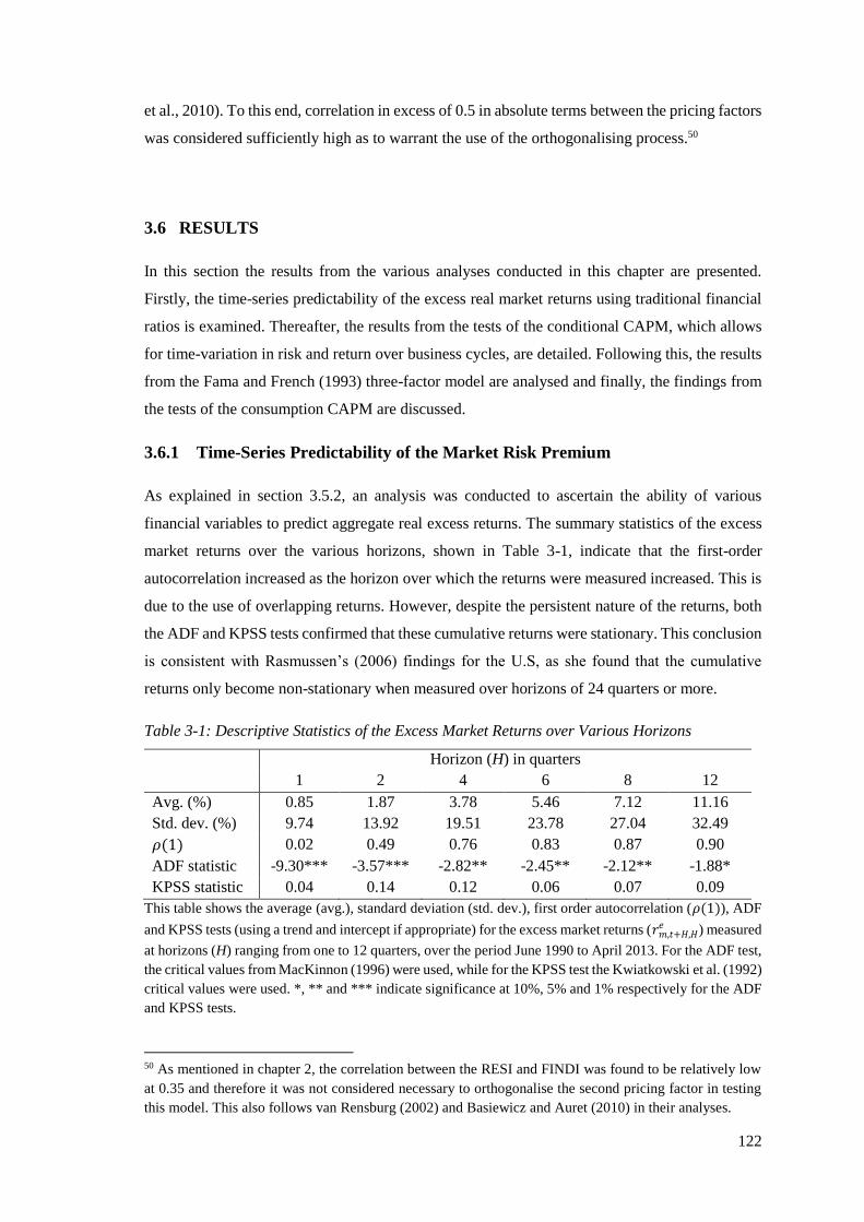
122

et al., 2010). To this end, correlation in excess of 0.5 in absolute terms between the pricing factors

was considered sufficiently high as to warrant the use of the orthogonalising process.50

3.6 RESULTS

In this section the results from the various analyses conducted in this chapter are presented.

Firstly, the time-series predictability of the excess real market returns using traditional financial

ratios is examined. Thereafter, the results from the tests of the conditional CAPM, which allows

for time-variation in risk and return over business cycles, are detailed. Following this, the results

from the Fama and French (1993) three-factor model are analysed and finally, the findings from

the tests of the consumption CAPM are discussed.

3.6.1 Time-Series Predictability of the Market Risk Premium

As explained in section 3.5.2, an analysis was conducted to ascertain the ability of various

financial variables to predict aggregate real excess returns. The summary statistics of the excess

market returns over the various horizons, shown in Table 3-1, indicate that the first-order

autocorrelation increased as the horizon over which the returns were measured increased. This is

due to the use of overlapping returns. However, despite the persistent nature of the returns, both

the ADF and KPSS tests confirmed that these cumulative returns were stationary. This conclusion

is consistent with Rasmussen’s (2006) findings for the U.S, as she found that the cumulative

returns only become non-stationary when measured over horizons of 24 quarters or more.

Table 3-1: Descriptive Statistics of the Excess Market Returns over Various Horizons

Horizon (H) in quarters

1 2 4 6 8 12

Avg. (%) 0.85 1.87 3.78 5.46 7.12 11.16

Std. dev. (%) 9.74 13.92 19.51 23.78 27.04 32.49

𝜌(1) 0.02 0.49 0.76 0.83 0.87 0.90

ADF statistic -9.30*** -3.57*** -2.82** -2.45** -2.12** -1.88*

KPSS statistic 0.04 0.14 0.12 0.06 0.07 0.09

This table shows the average (avg.), standard deviation (std. dev.), first order autocorrelation (𝜌(1)), ADF

and KPSS tests (using a trend and intercept if appropriate) for the excess market returns (𝑟𝑚,𝑡+𝐻,𝐻𝑒 ) measured

at horizons (H) ranging from one to 12 quarters, over the period June 1990 to April 2013. For the ADF test,

the critical values from MacKinnon (1996) were used, while for the KPSS test the Kwiatkowski et al. (1992)

critical values were used. *, ** and *** indicate significance at 10%, 5% and 1% respectively for the ADF

and KPSS tests.

50 As mentioned in chapter 2, the correlation between the RESI and FINDI was found to be relatively low

at 0.35 and therefore it was not considered necessary to orthogonalise the second pricing factor in testing

this model. This also follows van Rensburg (2002) and Basiewicz and Auret (2010) in their analyses.

123

The other four predictor variables exhibited substantial persistence (as shown in Table 3-2),

although the autocorrelation of 𝐷/𝑃 and 𝐸/𝑃 was lower than that documented for the U.S of more

than 0.9 (Lettau & Ludvigon, 2001a; Valkanov, 2003; Ang & Bekaert, 2007). The much shorter

time period examined in this study compared to the U.S research may explain this difference.

Both the ADF and KPSS tests revealed that these two series were stationary despite the reasonably

high level of persistence. 𝐷/𝑃 and 𝐸/𝑃 exhibited little variation over time, as captured by the

standard deviation measures, especially compared to the other two predictor variables as well as

the excess market returns.

Table 3-2: Summary Statistics of the Predictor Variables

𝑟𝑚𝑒 𝑟𝑒𝑙𝑎𝑡𝑖𝑣𝑒 𝑠𝑝𝑟𝑒𝑎𝑑 𝐷/𝑃 𝐸/𝑃

Panel A: Univariate Descriptive Statistics

Avg. 0.85 -0.53 0.98 -3.62 -2.67

Std. Dev. 9.74 2.09 1.69 0.21 0.20

𝜌(1) 0.02 0.83 0.85 0.84 0.84

ADF statistic -9.30*** -4.98*** -3.37** -3.99** -3.10**

KPSS statistic 0.04 0.05 0.11 0.09 0.07

Panel B: Correlation Matrix

𝑟𝑚𝑒 1

𝑟𝑒𝑙𝑎𝑡𝑖𝑣𝑒 -0.34 1

𝑠𝑝𝑟𝑒𝑎𝑑 0.30 -0.48 1

𝐷/𝑃 -0.35 -0.17 -0.31 1

𝐸/𝑃 -0.39 -0.11 -0.41 0.94 1

Panel A of this table shows the average (avg.), standard deviation (std. dev.), first order autocorrelation

(𝜌(1)), ADF and KPSS tests (using a trend and intercept if appropriate) for the five predictor variables -

the lagged excess market returns (𝑟𝑚𝑒 ), relative T-bill (𝑟𝑒𝑙𝑎𝑡𝑖𝑣𝑒), the term spread (𝑠𝑝𝑟𝑒𝑎𝑑), 𝐷/𝑃 and 𝐸/𝑃

- over the period June 1990 to April 2013. For the ADF test, the critical values from MacKinnon (1996)

were used, while for the KPSS test the Kwiatkowski et al. (1992) critical values were used. *, ** and ***

indicate significance at 10%, 5% and 1% respectively for these two tests. In panel B, the correlation

coefficients between the five predictor variables are presented.

Among the predictor variables, a strong positive relationship was evident between 𝐷/𝑃 and 𝐸/𝑃,

which is not surprising given the interconnectedness of dividends and earnings. A reasonably

strong negative relationship was also observed between the term spread and relative T-bill yield.

Again, this is not an unexpected finding given the similar inputs into their computation. The

spread, however, was more closely correlated with 𝐷/𝑃 and 𝐸/𝑃 than the relative T-bill yield.

The strength of some of these relationships certainly suggests that the variables may track

analogous components of the share returns.

The results from the predictive regressions are shown in Table 3-3. The lagged market return had

no ability to forecast future returns irrespective of the time-horizon. This result is consistent with

the low autocorrelation in the series and indicates that there was no evidence of mean reversion

over time. As mentioned in section 3.2.1.3, the U.S evidence is mixed with regards to the

124

Table 3-3: Forecasts of Multiple Quarter Excess Real Market Returns

Regressors Forecast horizon (H) in quarters

1 2 4 6 8 12

𝑟𝑚𝑒 0.02

(0.22)

[-0.01]

{0.00}

-0.06

(-0.04)

[-0.01]

{0.00}

0.51

(0.30)

[-0.01]

{0.00}

-1.09

(-0.51)

[-0.01]

{0.00}

-0.63

(-0.25)

[-0.01]

{0.00}

-1.72

(-0.60)

[-0.00]

{0.00}

𝑟𝑒𝑙𝑎𝑡𝑖𝑣𝑒 -2.06**

(-2.12)

[0.04]

{0.04}

-2.62

(-1.46)

[0.03]

{0.00}

-4.14

(-1.50)

[0.04]

{0.04}

-7.01*

(-1.92)

[0.08]

{0.02}

-10.49**

(-2.47)

[0.15]

{0.04}

-9.79*

(-1.72)

[0.09]

{0.01}

𝑠𝑝𝑟𝑒𝑎𝑑 1.98*

(1.86)

[0.04]

{0.04}

2.26

(1.33)

[0.02]

{0.04}

3.18

(1.10)

[0.02]

{0.00}

4.68

(1.31)

[0.03]

{0.00}

4.09

(1.07)

[0.01]

{0.00}

-3.37

(-0.71)

[-0.00]

{0.01}

𝐷/𝑃 1.41

(1.55)

[0.01]

{0.05}

2.92*

(1.94)

[0.03]

{0.05}

5.59**

(2.47)

[0.07]

{0.07}

8.42**

(2.56)

[0.12]

{0.05}

11.21***

(2.77)

[0.20]

{0.06}

20.86***

(4.87)

[0.44]

{0.03}

𝐸/𝑃 0.99

(1.13)

[-0.00]

{0.01}

2.07

(1.41)

[0.01]

{0.06}

3.60*

(1.74)

[0.02]

{0.07}

5.60*

(1.85)

[0.05]

{0.07}

8.34**

(2.09)

[0.09]

{0.03}

18.73***

(4.37)

[0.35]

{0.02}

𝑟𝑒𝑙𝑎𝑡𝑖𝑣𝑒

𝑠𝑝𝑟𝑒𝑎𝑑

𝐷/𝑃

-0.53

(-0.43)

2.34*

(1.83)

2.05*

(1.81)

[0.06]

{0.06}

-0.29

(-0.11)

3.33

(1.25)

3.91

(1.61)

[0.07]

{0.05}

-0.20

(-0.06)

5.37

(1.50)

7.24**

(2.20)

[0.13]

{0.07}

-1.55

(-0.50)

7.23*

(1.96)

10.43***

(2.68)

[0.22]

{0.06}

-6.18*

(-1.83)

4.57

(1.51)

11.57***

(2.76)

[0.29]

{0.04}

-6.89*

(-1.69)

-1.08

(-0.42)

19.19***

(4.47)

[0.46]

{0.04}

This table shows the coefficients from the predictive regressions of 𝑟𝑚,𝑡+𝐻,𝐻𝑒 = 𝜅𝐻′𝑧𝑡 + 휀1,𝑡+𝐻,𝐻 estimated

over the period June 1990 to April 2013, where 𝑟𝑚,𝑡+𝐻,𝐻𝑒 are the real excess market returns at horizon H

and 𝑧𝑡 is the column vector of predictor variables. The first five regressions were bivariate regressions

where 𝑧𝑡 included only the lagged excess market returns (𝑟𝑚𝑒 ), relative T-bill (𝑟𝑒𝑙𝑎𝑡𝑖𝑣𝑒), the term spread

(𝑠𝑝𝑟𝑒𝑎𝑑), 𝐷/𝑃 and 𝐸/𝑃, while the sixth regression was a multivariate regression where 𝑧𝑡 included 𝐷/𝑃,

𝑟𝑒𝑙𝑎𝑡𝑖𝑣𝑒 and 𝑠𝑝𝑟𝑒𝑎𝑑. Beneath each coefficient in round parentheses is the t-statistic computed using the

Newey and West (1987) standard errors. The regression 𝑅2, adjusted for degrees of freedom, ��2, is shown

in square parentheses, with Hodrick’s (1992) ��2 presented thereunder in curly parentheses. *, ** and ***

indicate significance at 10%, 5% and 1% respectively for the t-tests.

predictive power of the lagged market return, as although the early work of Fama and French

(1988b) and Lettau and Ludvigson (2001a) found significant univariate forecasting power, the

more recent findings of Lettau and Ludvigson (2010) contradict this. The relative T-bill yield was

identified to have predictive power on the JSE for one-quarter ahead and then for horizons longer

than six quarters. In contrast, the term spread only had significant (at 10%) predictive power for

125

one-quarter ahead returns; however, the finding that this variable was more closely related to

short-term rather than long-term business cycles is similar to Fama and French’s (1989) results.

The signs for both variables were consistent with the view that spreads and short-term interest

rates are positively and negatively correlated respectively with future business conditions. As

documented previously, Gupta and Modise (2012b, 2013) found that the term spread and relative

T-bill had predictive power for returns in South Africa and thus the findings from this analysis

are consistent with their results. Moreover, Gupta and Modise (2012b, 2013) also noted that the

term spread’s forecasting ability was limited to short-run horizons, while the relative T-bill was

able to predict returns at both short- and long-horizons (although in this study it was less

successful at two and four quarters ahead). The term spread and relative T-bill yield could explain

approximately 4% of the variation in returns in one-quarter ahead, as measured by ��2, and

Hodrick’s (1992) ��2 confirmed that the explanatory power of these variables was not inflated by

any persistence in these forecasting variables. Although this explanatory power is low, it is

comparable to international studies such as Lettau and Ludvigson (2010), who found that the

relative T-bill yield, for example, could explain 6% of the one-quarter ahead variation in returns,

with this declining as the forecast horizon increased (based on Hodrick’s, 1992 ��2).

𝐷/𝑃 and 𝐸/𝑃 were found to exhibit no forecasting power over a one-quarter horizon; however,

over longer horizons both financial ratios were seen to be significant predictors of returns, with

positive coefficients consistent with the view that these ratios move with future business cycles.

The ��2 values confirmed that for periods longer than four quarters, these two variables could

explain a substantial component of the variation in the future risk premium. However, Hodrick’s

(1992) ��2 values provide contradictory evidence, as they indicate that neither ratio could capture

substantial variation in returns. These results thus reveal that the significance of the coefficients

of the predictive regressions and high ��2 estimates using 𝐷/𝑃 and 𝐸/𝑃 may be a statistical

artefact arising from the persistence of these ratios. The finding of limited forecasting power for

these two ratios mirrors the results of Gupta and Modise (2012a) based on their bootstrapping

procedure. Moreover, this is also broadly consistent with the findings in the U.S after adjusting

for the near unit root processes of 𝐷/𝑃 and 𝐸/𝑃.

The fact that 𝐷/𝑃 does not contain useful information about future share returns on the JSE would

appear inconsistent with the theoretical framework of Campbell and Shiller (1989) outlined in

section 3.2.1.3. However, as Cochrane (2008b) explained, this may be a consequence of not

testing the full null hypothesis that if there is no predictive ability for 𝐷/𝑃, dividend growth must

be forecastable so as to explain variation in the ratio over time. Whether this is true for South

Africa, as Cochrane (2008b) found to be the case for the U.S is not known, as no explicit analysis

thereof has been conducted.

126

As mentioned in section 3.5.2, the joint predictive power of the forecasting variables in this

sample was also assessed, with the results thereof shown in the final row of Table 3-3.51 The

results highlight that the spread, relative T-bill yield and 𝐷/𝑃 contained different information

about future returns as at several horizons more than one variable was significant. A rather

surprising finding was that the 𝐷/𝑃 ratio was insignificant when analysed individually but

significant in the presence of the other variables at one-quarter ahead, while the same was true for

the term spread at six-quarters ahead. This does suggest that the predictor variables do move

together over time and are not completely orthogonal. The relative T-bill became insignificant at

one and six-quarters ahead compared to when analysed individually suggesting that some of the

information about future business cycles contained in this variable is captured in either the term

spread or 𝐷/𝑃 ratio. However, it remained significant at horizons of eight and 12-quarters. Gupta

and Modise (2012b, 2013) found the term spread and relative T-bill contained different

information about future share returns on the JSE, with the findings of this study largely

consistent, even in the presence of the highly persistent 𝐷/𝑃 ratio. Jointly these variables were

able to explain 6% of the variation in the one-quarter ahead returns and 46% over 12 quarters.

However, after accounting for the persistent nature of the 𝐷/𝑃 ratio, the one-quarter ahead

variation was still 6% but the 12 quarter-ahead value fell to only 4%. Accordingly, this

combination of three variables only has limited ability to forecast future share returns in the long-

run, with more success at short horizons.

The results from this analysis thus mirror those of Gupta and Modise (2012a, 2012b, 2013) that

traditional financial variables only have limited ability to forecast South African share returns. At

face value this suggests that South African share returns cannot be predicted. However, as

Cochrane (2008a) documents in analysing similar U.S evidence, this may not be an accurate

conclusion as the results may rather be a function of the unsuitability of these financial ratios as

forecasting variables rather than the absence of predictability in returns. Accordingly, further

research is conducted in chapters 4 and 5 to identify alternative forecasting variables. Given the

relatively limited predictive ability of the financial ratios examined in this section, the conditional

CAPM was examined with all five ratios rather than only the best performing so as to ensure that

any results documented were not sensitive to the choice of the conditioning variable.

51 𝐸/𝑃 and 𝐷/𝑃 were not examined jointly because of their high correlation. Only the regression with 𝐷/𝑃

is shown, in the interests of brevity, as it was found to perform better than 𝐸/𝑃. The lagged market return

was excluded as the combination without this variable yielded higher explanatory power.

127

3.6.2 The Conditional CAPM

3.6.2.1 Cross-Sectional Regression Results

Prior to estimating the conditional CAPM, the correlation between the pricing factors was

assessed for each of the five variables. The correlation between the excess real market returns,

the one-period lagged conditioning variables and the scaled market returns were relatively low in

absolute terms (less than 0.33), as displayed in Table B-1 in the appendix (p. 325), and therefore

none of the factors were orthogonalised.

The cross-sectional explanatory power of the conditional CAPM on the size and value portfolios

varied quite markedly depending on the conditioning variable, as shown in Table 3-4. The lowest

��2 of 29% was obtained using the relative T-bill yield, which was only marginally higher than

the static CAPM on the JSE of 27% (from chapter 2), whereas at the other end of the spectrum,

the model using 𝐷/𝑃 was able to explain 66% of the variation across the portfolios. The same

ranking of models was obtained using AIC. Although Rasmussen (2006) used the consumption

CAPM as the base model for evaluating the role of various conditioning variables in explaining

the returns across size and value portfolios, her results also showed substantial variation in ��2

across the conditioning variables. Moreover, similarly to the results obtained in this study,

Rasmussen (2006) obtained the highest explanatory power of 58% for the model based on the

inverse of the 𝐷/𝑃 but only 15% for the relative T-bill yield. However, before drawing

conclusions about the validity of the model based on the explanatory power, it was necessary to

ascertain whether the estimated risk premia were significant and had signs consistent with theory.

To this end, the results in Table 3-4 indicate that, similarly to the models examined in the

preceding chapter, the intercept was positive and significant in each of the specifications, in

contrast to theory. In results mirroring those for the CAPM, the market risk premium was

significant and negative for four of the five specifications (the model using 𝐸/𝑃 being the

exception). The scaled market risk premium was only significant for the model based on the term

spread, but this coefficient was positive suggesting that the market beta did vary across the

business cycle and, consistent with previous findings, shares whose market risk was more highly

correlated with the business cycle generated a higher risk premium. The fact that this result was

obtained only using the term spread as the predictor of the market risk premium is consistent with

the results from the forecasting analysis, which showed that at the one-quarter ahead horizon this

variable did have some predictive ability for future returns. This finding of limited evidence of

time-variation in market risk may not necessarily indicate that risk does not vary over time but

rather that the predictors of fluctuations in business cycles are poor; a conclusion consistent with

the results from the forecasting analysis in the preceding section.

128

Table 3-4: Cross-Sectional Regression Results for the Conditional CAPM


𝑟𝑚𝑒 𝑠𝑝𝑟𝑒𝑎𝑑 𝑟𝑒𝑙𝑎𝑡𝑖𝑣𝑒 𝐷/𝑃 𝐸/𝑃 𝑟𝑚

𝑒 𝑠𝑝𝑟𝑒𝑎𝑑 𝑟𝑒𝑙𝑎𝑡𝑖𝑣𝑒 𝐷/𝑃 𝐸/𝑃

𝜆0 4.88

(2.91)***

{1.98}*

7.99

(5.13)***

{3.60}***

8.12

(5.38)***

{3.89}***

5.58

(3.86)***

{2.16}**

4.12

(2.76)***

{1.57}

4.85

(3.17)***

{2.81}***

4.60

(3.39)***

{2.80}***

3.40

(2.91)***

{2.54}**

2.62

(1.78)*

{1.70}*

2.58

(1.78)*

{1.71}*

𝜆𝑚 -5.87

(-2.90)***

{-1.97}*

-6.63

(-3.29)***

{-2.30}**

-7.26

(-3.72)***

{-2.67}***

-4.73

(-2.44)**

{-1.63}

-3.20

(-1.57)

{-0.89}

-3.34

(-1.50)

{-0.82}

-3.63

(-1.59)

{-0.85}

-2.48

(-1.24)

{-0.63}

-1.16

(-0.50)

{-0.29}

-1.21

(-0.53)

{-0.30}

𝜆𝑧𝑡 8.50

(3.20)***

{2.18}**

0.60

(1.22)

{0.85}

-0.79

(-1.32)

{-0.95}

-0.27

(-3.78)***

{-2.11}**

-0.29

(-4.23)***

{2.40}**

-3.98

(-0.82)

{-0.62}

-1.09

(-1.41)

(-0.99}

0.87

(0.45)

{0.37}

0.02

(0.40)

{0.24}

0.05

(0.88)

{0.53}

𝜆𝑚𝑡+1,𝑧𝑡 28.46

(1.20)

{0.82}

12.96

(3.58)***

{1.81}*

-6.67

(-1.16)

{-0.84}

0.38

(0.64)

{0.36}

-0.24

(-0.45)

{-0.26}

14.83

(0.69)

{0.36}

2.86

(0.53)

(0.30}

7.68

(0.61)

{0.47}

-0.41

(-0.52)

{-0.41}

0.14

(0.25)

{0.18}

𝑅2

(��2)

0.57

(0.47)

0.59

(0.49)

0.44

(0.29)

0.73

(0.66)

0.67

(0.59)

0.85

(0.75)

0.87

(0.78)

0.70

(0.52)

0.79

(0.66)

0.80

(0.68)

AIC 0.93 0.89 1.21 0.47 0.67 -1.73 -1.85 -1.07 -1.40 -1.48


{9.30}**

19.04***

{9.30}**

16.90***

{8.75**}

20.55***

{6.44}*

20.53***

{6.59*}

3.23

{1.14}

4.79

(1.81}

2.11

{0.75}

0.68

{0.31}

1.12

{0.41}

RMSE 1.20 1.18 1.38 0.95 1.06 0.42 0.51 0.48 0.40 0.42


{71.79}***

25.66**

{52.19}***

38.17***

{73.10}***

39.13***

{124.41}***

33.74***

{104.87}***

2.54

{3.25}

5.59

{6.46}

4.46

{5.89}

2.14

{2.35}

2.44

{2.63}

This table reports the coefficients from the Fama and MacBeth (1973) cross-sectional regression ��𝑖,𝑡+1𝑒 = 𝜆0 + 𝜆𝑓′𝛽

𝑖𝑓+ 𝜂

𝑖, estimated over the period June 1990 to April 2013

across the 16 size and value portfolios and nine industry portfolios, where 𝛽𝑖𝑓

is a column vector of the sensitivity of the portfolio returns (𝑟𝑖,𝑡+1𝑒 ) to the pricing factors obtained

from the time-series regressions. For the conditional CAPM, the factor loading was the sensitivity to the excess real market returns (𝛽𝑖𝑚

), the sensitivity to the conditioning

variable (𝛽𝑖𝑧

) and the sensitivity to the scaled excess market returns (𝛽𝑖𝑚𝑧

). The conditioning variable was measured by the lagged excess market returns (𝑟𝑚𝑒 ), relative T-bill

yield (𝑟𝑒𝑙𝑎𝑡𝑖𝑣𝑒), the term spread (𝑠𝑝𝑟𝑒𝑎𝑑), 𝐷/𝑃 and 𝐸/𝑃 in each of the five models. Beneath each coefficient in round parentheses is the t-statistic computed using the Fama

129

and MacBeth (1973) standard errors, while the second t-statistic in curly parentheses was calculated using the Shanken (1992) standard errors. The Wald statistic provides a test

of the joint significance of the coefficients and the Q-statistic tests the joint significance of the model pricing errors. The values of both of these statistics computed using

Shanken’s (1992) standard errors are shown in curly parentheses. RMSE refers to the root mean squared pricing error across the portfolios. The 𝑅2 is Jagannathan and Wang’s

(1996) cross-sectional measure of explanatory power and ��2 is adjusted for the number of pricing factors. The AIC refers to the Akaike information criteria and was computed

similarly to Jagannathan and Wang’s (1996) 𝑅2. *, ** and *** indicate significance at 10%, 5% and 1% respectively for the various tests conducted.

130

Turning to the conditional risk premium, the coefficients were significant for the lagged market

excess return, 𝐷/𝑃 and 𝐸/𝑃. This coefficient should be identical in sign to that obtained in the

forecasting equation (Li et al., 2011), but unlike the intertemporal CAPM this restriction is not

usually explicitly tested in the conditional CAPM, with several studies obtaining inconsistent

results in this regard (see for example Santos & Veronesi, 2006; Rasmussen, 2006). The lagged

market risk premium was found to exhibit no forecasting power and thus the finding of a positive

and significant coefficient on the lagged market risk premium in the cross-sectional regression is

surprising. This result possibly points to the fact that investors do not respond immediately to

changes in share prices giving rise to an intertemporal relationship between risk and return on the

JSE. This is consistent with the findings from the time-series tests of Basiewicz and Auret (2010)

who found that this factor played an important role in the CAPM.

To examine this relationship further, Figure 3-1 displays the lagged market betas for the 16

portfolios. These betas are much larger for the value portfolios than the growth portfolios,

suggesting that a portion of the value anomaly may be attributable to variation in returns across

the business cycle that may be a function of varying investment opportunities, risk not captured

by the contemporaneous market beta (but captured by the lagged market beta) or related to

smoothing consumption over time. However, as indicated in section 3.2.1.5, this measure does

not indicate which of these possible explanations is appropriate. In contrast there was no

consistent pattern across the size-sorted portfolios.

The significance of 𝐷/𝑃 and 𝐸/𝑃 in the cross-sectional regressions are similar to the finding from

the forecasting analysis52; however, the negative signs are contradictory not only with the

forecasting analysis but also with expectations that the returns to portfolios sorted by 𝐵/𝑀, a

closely related measure of value, are not positively correlated. Interestingly, Rasmussen (2006)

also found that the signs in the cross-sectional regression on these two conditioning variables

differed from those documented in the time-series regression; however, she did not draw attention

to this inconsistency or provide any rationale for it.

To try and understand this surprising relationship, some further analysis was performed. Firstly,

the one-period ahead predictive regression with each of these variables (equation 3.1) was

estimated for all 16 portfolios. Although the factor loadings were largely insignificant (13 for

𝐷/𝑃 and 14 for 𝐸/𝑃), Jagannathan et al. (1998) point out that this may arise not because of the

absence of a relationship but rather because the estimates are imprecise (measured with substantial

52 Their significance in the cross-sectional regression is unlikely to be a function of the near unit root

properties of D/P and 𝐸/𝑃 because this is reflected in the standard errors in the time-series regression and

not the coefficients which are used in this regression.

131

Figure 3-1: Conditional CAPM Betas for the Size and Value Portfolios

This figure plots the conditional beta (𝛽𝑖𝑧

) estimated from the time-series regression of 𝑟𝑖,𝑡+1𝑒 = 𝛼𝑖 +

𝛽𝑖𝑧

z𝑡 + 𝛽𝑖𝑚

𝑟𝑚,𝑡+1𝑒 + 𝛽

𝑖𝑚𝑧𝑟𝑚,𝑡+1

𝑒 z𝑡 + 휀𝑖,𝑡+1 over the period June 1990 to April 2013 for each of the 16 size

and value portfolios, where 𝑟𝑖,𝑡+1𝑒 are the excess portfolio returns, 𝑟𝑚,𝑡+1

𝑒 are the excess real market returns,

z𝑡 is the conditioning variable and 𝑟𝑚,𝑡+1𝑒 z𝑡 refers to the scaled market returns. For this model, the

conditioning variable was the lagged market return (𝑟𝑚,𝑡𝑒 ). S1 refers to the portfolios of large firms and S4

the portfolios of small firms while B1 refers to the portfolios of firms with high 𝐵/𝑀 ratios and B4 the

portfolios of firms with low 𝐵/𝑀 ratios.

error) and this was certainly found to be true with these regressions. Moreover, given that the

variation associated with the factor loadings is not considered in the computation of the cross-

sectional risk premium, it is plausible that although the time-series factor loadings may have been

insignificant for the majority of the portfolios, the risk factor may still be priced in the cross-

section, as was observed to be true here.

The returns on the portfolios comprising large firms exhibited a positive relationship with the

lagged 𝐷/𝑃 ratio which was consistent with the findings from the forecasting regression. This is

to be expected as the market return in that analysis was measured using the ALSI, with this index

dominated by large firms because of the concentration on the JSE. For the portfolios of smaller

firms, the opposite pattern emerged as negative factor loadings were obtained, suggesting that

small shares may act as a hedge against adverse market movements (a decrease in 𝐷/𝑃 signals a

market contraction in the future which is likely to be associated with lower returns). If they do act

as a hedge, then investors would not require a substantial risk premium to induce them to hold

these securities; yet this is precisely the opposite of what is seen as the small firm portfolio earned

more than those holding large firms; thus giving rise to the negative cross-sectional risk premium

estimate. Accordingly, despite the variation in the betas across the different sized portfolios, the

results do not make economic sense. Interestingly to note, when the market factor was added to

132

the regression, the positive relationship observed between the large firm portfolio returns and the

𝐷/𝑃 became negative. This change in sign cannot be attributed to high correlation between the

two factors (as documented previously) and thus speaks to a model with important factors missing

as such changes in sign should not occur in a well-specified model. Thus, this finding of a

significant negative risk premium on 𝐷/𝑃 and 𝐸/𝑃 is difficult to reconcile with theory, thus

bringing the validity of the model as a means of explaining returns across portfolios into question.

The final analysis of the suitability of the conditional CAPM in explaining the variation across

the size- and value-sorted portfolios was based on the pricing errors. As shown in Table 3-4, the

RMSEs for the conditional models were lower than the CAPM of 1.55, with the model including

the 𝐷/𝑃 performing the best with an RMSE of only 0.95. The latter result is thus consistent with

the findings from the goodness of fit statistics but does not reflect the a-theoretical findings from

the coefficient estimates. However, despite these comparatively low estimates, the Q-statistics

confirmed that the pricing errors remained significant under all the conditional specifications. To

examine the patterns in the pricing errors, the errors from the conditional CAPM with the lagged

market return (the model with the most plausible coefficient estimates) are depicted in Figure 3-

2. As can be seen, the portfolios are more closely clustered around the 45-degree line than was

the case for the CAPM (shown in Figure 2-3). However, the portfolios with the largest mispricing

remained the small firm portfolios and those comprising value and growth shares.

The explanatory power of the conditional CAPM for JSE-listed firms does exceed estimates

obtained for the model from U.S studies. For example, in the studies of Kullmann (2003) and

Jagannathan and Wang (1996), the model was only able to explain 25% and 30% of the variation

in portfolio returns respectively. However, there are several possible reasons for the higher

explanatory power observed in this market. Most notable of these is the fact that the market risk

premium was found to be significant in this sample and thus although the sign is inconsistent with

theory, the fact that the risk premium is priced in contrast to the U.S studies contributes to the

higher explanatory power. Different model specifications (Kullmann, 2003; Jagannathan &

Wang, 1996 both only included a time-varying return component whereas both a time-varying

return and market risk parameter were included in this study) and the use of different portfolios

(both the U.S studies tested the model on size and beta-sorted portfolios as opposed to the size-

and value-sorted portfolios used in this study) may also account for the differences observed.

For the industry portfolios, the ��2 estimates ranged between 52% and 78% with the relative T-

bill yield again the least successful conditioning variable, although for this set of portfolios, the

term spread was the most successful compared to the 𝐷/𝑃 ratio for the size- and value-sorted

portfolios. The pricing errors for the model were low and insignificant. However, as with the

CAPM and two-factor model, the slope coefficients were all insignificant indicating that the

133

model did not capture the cross-sectional variation in these portfolio returns. Thus, the high ��2,

low information criteria and insignificant pricing errors are a consequence of the relatively low

variation across the portfolios rather than the good fit of the models.

Figure 3-2: Pricing Errors from the Conditional CAPM for the Size and Value Portfolios

This figure plots the pricing errors from the cross-sectional regression ��𝑖,𝑡+1

𝑒 = 𝜆0 + 𝜆z𝛽𝑖𝑧

+ 𝜆𝑖𝛽𝑖𝑚+

𝜆𝑖𝑚𝑧𝛽𝑖𝑚𝑧

+ 𝜂𝑖 over the period June 1990 to April 2013 across the 16 size and value portfolios, where ��𝑖,𝑡+1

𝑒

are the average excess portfolio returns and 𝛽𝑖𝑚

, 𝛽𝑖𝑧

and 𝛽𝑖𝑚𝑧

measure the sensitivity of the portfolio returns

to the excess real market returns, conditioning variable and the scaled excess market returns respectively.

For this model, the conditioning variable was the lagged market return. S1 refers to the portfolios of large

firms and S4 the portfolios of small firms while B1 refers to the portfolios of firms with high 𝐵/𝑀 ratios

and B4 the portfolios of firms with low 𝐵/𝑀 ratios.

3.6.2.2 GMM Regression Results

The results of the GMM regressions are shown in Table 3-5. The beta on the conditioning variable

and the implied risk premium on this factor loading were significant in the SDF and return-beta

linear equation when the market risk premium, 𝐷/𝑃 and 𝐸/𝑃 ratios were used as the conditioning

variables, showing that these factors help to price securities. The risk premia on 𝐷/𝑃 and 𝐸/𝑃,

however, entered with an incorrect sign. The lagged market risk premium was positive and

significant. These results thus mirror those documented in Table 3-4 and again point to an

important role for the lagged market risk premium. The conditional market risk premium was

again priced when the spread was used to condition the returns, while compared to the cross-

sectional results, the transformed conditional market risk premium was also significant in the

equations for the relative T-bill yield and the 𝐷/𝑃 ratio. The conditioned market risk premium

was also found to help price the securities in the presence of the other variables, as shown by the

significant coefficients in the SDF. The conditional market risk premium on the relative T-bill

entered with the wrong sign but that on the 𝐷/𝑃 ratio did enter with the correct positive sign.

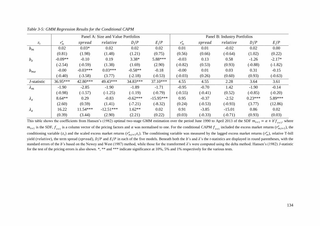
134

Table 3-5: GMM Regression Results for the Conditional CAPM

𝑧𝑡


𝑟𝑚𝑒 𝑠𝑝𝑟𝑒𝑎𝑑 𝑟𝑒𝑙𝑎𝑡𝑖𝑣𝑒 𝐷/𝑃 𝐸/𝑃 𝑟𝑚

𝑒 𝑠𝑝𝑟𝑒𝑎𝑑 𝑟𝑒𝑙𝑎𝑡𝑖𝑣𝑒 𝐷/𝑃 𝐸/𝑃

𝑏𝑚 0.02

(0.81)

0.03*

(1.98)

0.02

(1.48)

0.02

(1.21)

0.02

(0.75)

0.01

(0.56)

0.01

(0.66)

-0.02

(-0.64)

0.02

(1.02)

0.00

(0.22)

𝑏𝑧 -0.09**

(-2.54)

-0.10

(-0.59)

0.19

(1.38)

3.38*

(1.69)

5.88***

(2.90)

-0.03

(-0.82)

0.13

(0.53)

0.58

(0.93)

-1.26

(-0.88)

-2.17*

(-1.82)

𝑏𝑚𝑧 -0.00

(-0.40)

-0.03***

(-3.58)

0.03***

(3.77)

-0.58**

(-2.18)

-0.18

(-0.53)

-0.00

(-0.03)

0.01

(0.26)

0.03

(0.60)

0.31

(0.93)

-0.15

(-0.63)

J-statistic 36.95*** 42.80*** 49.43*** 34.83*** 37.10*** 4.55 4.55 2.28 3.64 3.61

𝜆𝑚 -1.90

(-0.98)

-2.85

(-1.57)

-1.90

(-1.25)

-1.89

(-1.19)

-1.71

(-0.79)

-0.95

(-0.55)

-0.70

(-0.41)

1.42

(0.52)

-1.90

(-0.85)

-0.14

(-0.20)

𝜆𝑧 8.64**

(2.60)

0.29

(0.59)

-0.83

(1.41)

-0.62***

(-7.21)

-15.95***

(-8.32)

0.95

(0.24)

-0.37

(-0.53)

-2.52

(-0.93)

0.23***

(3.77)

5.89***

(12.86)

𝜆𝑧 16.22

(0.39)

11.54***

(3.44)

-12.51***

(2.90)

1.62**

(2.21)

0.02

(0.22)

0.91

(0.03)

-3.85

(-0.33)

-15.01

(-0.71)

0.86

(0.93)

0.02

(0.03)

This table shows the coefficients from Hansen’s (1982) optimal two-stage GMM estimation over the period June 1990 to April 2013 of the SDF 𝑚𝑡+1 = 𝛼 + 𝑏′𝑓𝑡+1

, where

𝑚𝑡+1 is the SDF, 𝑓𝑡+1

is a column vector of the pricing factors and 𝛼 was normalised to one. For the conditional CAPM 𝑓𝑡+1

included the excess market returns (𝑟𝑚,𝑡+1𝑒 ), the

conditioning variable (𝑧𝑡) and the scaled excess market returns (𝑟𝑚,𝑡+1𝑒 𝑧𝑡). The conditioning variable was measured by the lagged excess market returns (𝑟𝑚

𝑒 ), relative T-bill

yield (𝑟𝑒𝑙𝑎𝑡𝑖𝑣𝑒), the term spread (𝑠𝑝𝑟𝑒𝑎𝑑), 𝐷/𝑃 and 𝐸/𝑃 in each of the five models. Beneath both the 𝑏’s and 𝜆’s the t-statistics are displayed in round parentheses, with the

standard errors of the 𝑏’s based on the Newey and West (1987) method, while those for the transformed 𝜆’s were computed using the delta method. Hansen’s (1982) J-statistic

for the test of the pricing errors is also shown. *, ** and *** indicate significance at 10%, 5% and 1% respectively for the various tests.

135

Thus, in contrast to the time-varying return component where 𝐷/𝑃 cannot appropriately explain

differences in returns, the evidence from the GMM output shows that the ratio can capture a

component of the future business cycles when conditioned on market risk, as with the term spread.

Similarly to the cross-sectional results, the pricing errors of each of these models remained

significant, as reflected by the J-statistics.

For the industry-sorted portfolios, the GMM results were identical to those from the cross-

sectional regressions with all the pricing factors insignificant, except for the coefficients on 𝐷/𝑃

and 𝐸/𝑃, as shown in Table 3-5. This is similar to what was found for the size and value

portfolios; however, the notable difference is the fact that the risk premia on these two factors

enter with positive coefficients, in accordance with theory that those portfolios which are highly

correlated with future business cycles should earn higher returns.

With regards to the importance of the time-varying coefficients, the results in this study vary quite

markedly depending on the conditioning variable used, which makes drawing definitive

conclusions difficult. Overall, more evidence exists to suggest that time-varying returns rather

than time-varying market risk are important in explaining the cross-sectional variation in returns

across the size and value portfolios, but as mentioned, this may be a function of the lack of a

suitable forecasting variable. While the model does result in higher explanatory power than the

CAPM, the model still yields risk premia estimates which are inconsistent with theory. However,

the relative success of the conditional CAPM when the lagged market return was used

demonstrates that part of the reason for the poor performance of the CAPM may be a function of

time-varying returns.

3.6.3 The Fama and French (1993) Three-Factor Model

3.6.3.1 Time-Series Regression Results

Prior to estimating the Fama and French (1993) model, the correlation between the three factors

was examined. SMB and HML had a relatively low correlation of -0.27, as shown in Table 3-6,

with the negative sign consistent with most international evidence. Although the magnitude of

this relationship is higher than Fama and French (1993) for the U.S of -0.08 and Nartea et al.

(2009) for New Zealand of -0.12; it is comparable to that documented by Brailsford et al. (2012)

of -0.31 for Australia and indicates that the HML and SMB factors are largely free of the effects

of size and value respectively. HML exhibited little co-movement with the market, whereas SMB

moved in the opposite direction to the market, with a correlation coefficient of -0.44. Fama and

French (1993) found that the relationship of both portfolios with the market was sizable but with

the opposite signs to those observed for the South African series. The strong negative relationship

between SMB and the market risk premium could be explained by the fact that the South African

136

Table 3-6: Correlation Matrix of the Pricing Factors in the CAPM and Two-Factor Model

𝑟𝑚𝑒 𝐻𝑀𝐿 𝑆𝑀𝐵

𝑟𝑚𝑒 1

𝐻𝑀𝐿 0.05 1

𝑆𝑀𝐵 -0.40 -0.27 1

This table shows the correlation coefficients between the excess market return (𝑟𝑚𝑒 ), HML and SMB for the

period June 1990 to April 2013.

market portfolio is more heavily weighted towards large shares because of the degree of

concentration on the JSE (as mentioned in the previous chapter).

The risk premia implied from the time-series averages of the three factors are shown in Table 3-

7. SMB and HML earned positive and significant premia over the period that were much larger

than the market risk premium. These results confirm the patterns identified in chapter 2 of the

presence of strong size and value premia on the JSE.

Table 3-7: Time-Series Estimates of the Factor Risk Premia for the Fama and French (1993)

Model

𝜆𝑚 𝜆𝑆𝑀𝐵 𝜆𝐻𝑀𝐿

𝜆𝑓

t-statistic

0.85

(0.83)

2.13**

(2.19)

2.43***

(2.71)

In this table the factor risk premia (𝜆𝑓) for the market (𝜆𝑚), SMB (𝜆𝑆𝑀𝐵) and HML (𝜆𝐻𝑀𝐿) are shown. These

are estimated as the time-series average, 𝐸𝑡(𝑓), for the period June 1990 to April 2013. Beneath each

coefficient the t-statistic computed using the Newey and West (1987) standard errors is shown in round

parentheses. *, ** and *** indicate significance at 10%, 5% and 1% respectively for the t-tests.

The summary results from the time-series regressions of this model are shown in Table 3-8, with

the full results documented in Tables B-2 and B-3 in the appendix for the size- and value-sorted

and industry-sorted portfolios respectively (p. 325 and p. 326 respectively). The evidence from

the first sample provides a sharp contrast to that obtained for the portfolio-based models examined

previously as none of the intercepts were individually significant at 5% (only one at 10%) and

jointly they were also not significantly different to zero. These size- and value-sorted portfolios

thus earned a return commensurate with their level of risk over time, where risk is measured by

the sensitivity to the market, SMB and HML. This success of the three-factor model in time-series

tests on the JSE is consistent with the international evidence documented previously (Fama &

French, 1993, 1996 for the U.S; Brailsford et al., 2012 for Australia).

As mentioned in section 3.3.2., for South Africa, Basiewicz and Auret (2010) also failed to reject

the joint test of the significance of the pricing errors from the three-factor model. However, they

observed that while the model could explain the value anomaly, it had less success with the size

anomaly. Although there was some evidence of the same pattern in this study (the weakly

significant coefficient was that of a portfolio of small shares, as shown in Table B-2), overall the

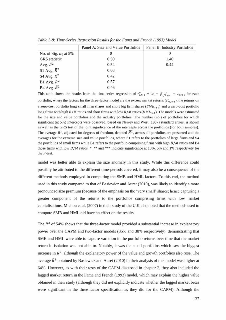
137

Table 3-8: Time-Series Regression Results for the Fama and French (1993) Model


No. of Sig. 𝛼𝑖 at 5% 0 0

GRS statistic 0.50 1.40

Avg. ��2 0.54 0.44

S1 Avg. ��2 0.68

S4 Avg. ��2 0.42

B1 Avg. ��2 0.57

B4 Avg. ��2 0.46

This table shows the results from the time-series regression of 𝑟𝑖,𝑡+1𝑒 = 𝛼𝑖 + 𝛽

𝑖𝑓𝑓

𝑡+1+ 휀𝑖,𝑡+1 for each

portfolio, where the factors for the three-factor model are the excess market returns (𝑟𝑚,𝑡+1𝑒 ), the returns on

a zero-cost portfolio long small firm shares and short big firm shares (𝑆𝑀𝐵𝑡+1) and a zero-cost portfolio

long firms with high 𝐵/𝑀 ratios and short firms with low 𝐵/𝑀 ratios (𝐻𝑀𝐿𝑡+1). The models were estimated

for the size and value portfolios and the industry portfolios. The number (no.) of portfolios for which

significant (at 5%) intercepts were observed, based on Newey and West (1987) standard errors, is shown

as well as the GRS test of the joint significance of the intercepts across the portfolios (for both samples).

The average 𝑅2, adjusted for degrees of freedom, denoted ��2, across all portfolios are presented and the

averages for the extreme size and value portfolios, where S1 refers to the portfolios of large firms and S4

the portfolios of small firms while B1 refers to the portfolio comprising firms with high 𝐵/𝑀 ratios and B4

those firms with low 𝐵/𝑀 ratios. *, ** and *** indicate significance at 10%, 5% and 1% respectively for

the F-test.

model was better able to explain the size anomaly in this study. While this difference could

possibly be attributed to the different time-periods covered, it may also be a consequence of the

different methods employed in computing the SMB and HML factors. To this end, the method

used in this study compared to that of Basiewicz and Auret (2010), was likely to identify a more

pronounced size premium (because of the emphasis on the ‘very small’ shares; hence capturing a

greater component of the returns to the portfolios comprising firms with low market

capitalisations. Michou et al. (2007) in their study of the U.K also noted that the methods used to

compute SMB and HML did have an effect on the results.

The ��2 of 54% shows that the three-factor model provided a substantial increase in explanatory

power over the CAPM and two-factor models (35% and 38% respectively), demonstrating that

SMB and HML were able to capture variation in the portfolio returns over time that the market

return in isolation was not able to. Notably, it was the small portfolios which saw the biggest

increase in ��2, although the explanatory power of the value and growth portfolios also rose. The

average ��2 obtained by Basiewicz and Auret (2010) in their analysis of this model was higher at

64%. However, as with their tests of the CAPM discussed in chapter 2, they also included the

lagged market return in the Fama and French (1993) model, which may explain the higher value

obtained in their study (although they did not explicitly indicate whether the lagged market betas

were significant in the three-factor specification as they did for the CAPM). Although the

138

explanatory power of the model on the South African market was lower than that on the U.S

market where Fama and French (1993, 1996) obtained ��2 values in excess of 90%, it was

equivalent to that obtained on the Australian market, as documented by Brailsford et al. (2012).

With the industry portfolios, the individual and joint significance tests all resulted in the same

conclusion that the pricing errors were equal to zero. This result, however, is similar to that

observed for the other models thus far in this study, but also closely mirrors the findings of Li

(2010) for the Australian market for the three-factor model tested on industry-sorted portfolios.

The average ��2 of 44% was higher than the CAPM (37%), suggesting that SMB and HML were

able to explain a larger proportion of the variation in the industry portfolio returns over time than

the market return alone, but the model was less successful than the two-factor model (��2 of 54%),

as noted in chapter 2.


The results from the second-pass regression for the three-factor model are shown in Table 3-9.

The ��2 of 70% for the model on the size and value portfolios demonstrates that this model was

able to explain a substantial component of the variation across these portfolios. This provides a

substantial improvement to the 27% for the CAPM. This cross-sectional ��2 is almost identical to

that obtained by Basiewicz (2007) in his unpublished study of the model in South Africa;

confirming that the use of quarterly as opposed to monthly data, with the consequent reduction in

the number of time-series observations, did not bias the results obtained. The explanatory power

is also equivalent to that documented by Lettau and Ludvigson (2001b) and Funke et al. (2010)

on the U.S market, who found that the three-factor model was able to explain approximately 75%

of the cross-sectional variation for the size- and value-sorted portfolios, and exceeds the value of

42% obtained by Li et al. (2011) for Australia. The slope coefficients were positive and significant

for HML and SMB, based on the adjusted and unadjusted t-statistics; consistent with the intuition

that portfolios which had higher sensitivities to SMB and HML yielded higher returns. In addition,

it was also found that these risk premia did not differ significantly from the observed premia to

the SMB and HML factors. Basiewicz (2007) only found the value factor to be significant;

however, this difference regarding the importance of size in explaining the cross-sectional

variation may be attributable to the different formulations of the size factor, as highlighted

previously. The fact that SMB is significant in this study again points to the fact that the size

effect on the JSE is concentrated within the ‘very small’ shares. In the U.S, there has been some

evidence to suggest that size is not priced (as the anomaly has attenuated in recent years, as

documented in chapter 2) (see Lettau & Ludvigson, 2001b; Funke et al., 2010), but the evidence

obtained for the JSE in this study that both factors were significant is similar to Australia (Li et

al., 2011).

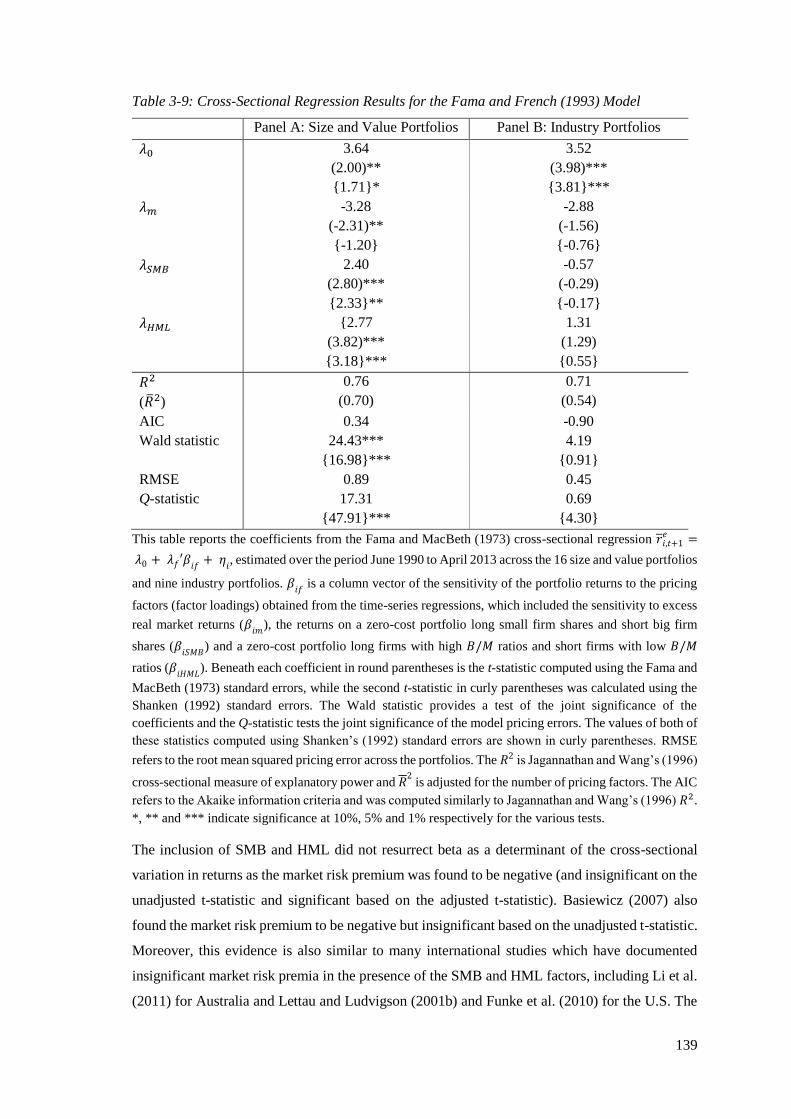
139

Table 3-9: Cross-Sectional Regression Results for the Fama and French (1993) Model


𝜆0 3.64

(2.00)**

{1.71}*

3.52

(3.98)***

{3.81}***

𝜆𝑚 -3.28

(-2.31)**

{-1.20}

-2.88

(-1.56)

{-0.76}

𝜆𝑆𝑀𝐵 2.40

(2.80)***

{2.33}**

-0.57

(-0.29)

{-0.17}

𝜆𝐻𝑀𝐿 {2.77

(3.82)***

{3.18}***

1.31

(1.29)

{0.55}

𝑅2

(��2)

0.76

(0.70)

0.71

(0.54)

AIC 0.34 -0.90


{16.98}***

4.19

{0.91}

RMSE 0.89 0.45

Q-statistic 17.31

{47.91}***

0.69

{4.30}


𝜆0 + 𝜆𝑓′𝛽𝑖𝑓

+ 𝜂𝑖, estimated over the period June 1990 to April 2013 across the 16 size and value portfolios

and nine industry portfolios. 𝛽𝑖𝑓

is a column vector of the sensitivity of the portfolio returns to the pricing

factors (factor loadings) obtained from the time-series regressions, which included the sensitivity to excess

real market returns (𝛽𝑖𝑚

), the returns on a zero-cost portfolio long small firm shares and short big firm

shares (𝛽𝑖𝑆𝑀𝐵

) and a zero-cost portfolio long firms with high 𝐵/𝑀 ratios and short firms with low 𝐵/𝑀

ratios (𝛽𝑖𝐻𝑀𝐿

). Beneath each coefficient in round parentheses is the t-statistic computed using the Fama and

MacBeth (1973) standard errors, while the second t-statistic in curly parentheses was calculated using the

Shanken (1992) standard errors. The Wald statistic provides a test of the joint significance of the

coefficients and the Q-statistic tests the joint significance of the model pricing errors. The values of both of

these statistics computed using Shanken’s (1992) standard errors are shown in curly parentheses. RMSE

refers to the root mean squared pricing error across the portfolios. The 𝑅2 is Jagannathan and Wang’s (1996)

cross-sectional measure of explanatory power and ��2 is adjusted for the number of pricing factors. The AIC

refers to the Akaike information criteria and was computed similarly to Jagannathan and Wang’s (1996) 𝑅2.

*, ** and *** indicate significance at 10%, 5% and 1% respectively for the various tests.

The inclusion of SMB and HML did not resurrect beta as a determinant of the cross-sectional

variation in returns as the market risk premium was found to be negative (and insignificant on the

unadjusted t-statistic and significant based on the adjusted t-statistic). Basiewicz (2007) also

found the market risk premium to be negative but insignificant based on the unadjusted t-statistic.

Moreover, this evidence is also similar to many international studies which have documented

insignificant market risk premia in the presence of the SMB and HML factors, including Li et al.

(2011) for Australia and Lettau and Ludvigson (2001b) and Funke et al. (2010) for the U.S. The

140

Wald test statistic was significant, confirming that the three pricing factors jointly were able to

explain the variation across the portfolios. The intercept of the model, however, remained

significant and positive, in contrast to theory, with the magnitude too high to reconcile with the

argument of the incorrect measure of the risk-free rate. Given that the market portfolio proxy is

included as a pricing factor in this model, the possibility remains that this high intercept may be

a consequence of the use of a proxy that is not mean-variance efficient.

The pricing errors from the model were insignificant based on the unadjusted standard errors but

significant based on the adjusted values, as indicated by the Q-statistics in Table 3-9. Thus, there

was some evidence to suggest that the model was able to explain the differences in returns across

these portfolios. Lettau and Ludvigson (2001b) for the U.S and Li et al. (2011) for Australia found

that the model still yielded substantial pricing errors. The pricing errors for the portfolios, shown

in Figure 3-3, plot substantially closer to the 45-degree line than those obtained for any of the

other models examined thus far in this study. However, this graph also confirms that the three-

factor model still had some difficulty in explaining the returns to the portfolios comprising small

shares (similarly to Lettau & Ludvigson, 2001b), with some discrepancies also evident with the

value and growth shares.

Figure 3-3: Pricing Errors from the Fama and French (1993) Model for the Size and Value

Portfolios

This figure plots the pricing errors from the cross-sectional regression ��𝑖,𝑡+1𝑒 = 𝜆0 + 𝜆𝑚𝛽

𝑖𝑚+

𝜆𝑆𝑀𝐵𝛽𝑖𝑆𝑀𝐵

+ 𝜆𝐻𝑀𝐿𝛽𝑖𝐻𝑀𝐿

+ 𝜂𝑖 over the period June 1990 to April 2013 across the 16 size and value

portfolios, where 𝛽𝑖𝑚

, 𝛽𝑖𝑆𝑀𝐵

and 𝛽𝑖𝐻𝑀𝐿

measure the sensitivity of the portfolio returns to the excess real

market returns, the returns on a zero-cost portfolio long small firm shares and short big firm shares and a

zero-cost portfolio long firms with high 𝐵/𝑀 ratios and short firms with low 𝐵/𝑀 ratios. S1 refers to the

portfolios of large firms and S4 the portfolios of small firms while B1 refers to the portfolios of firms with

high 𝐵/𝑀 ratios and B4 the portfolios of firms with low 𝐵/𝑀 ratios.

141

The three-factor model explained 54% of the variation across the industry-sorted portfolios;

however, as shown in Table 3-9, the pricing factors were all insignificant. The finding of an

insignificant market risk premium is consistent with previous findings on this sample, but those

for SMB and HML suggest that the extent to which these two portfolios were able to explain

variation across portfolios was limited to the size and value groupings. Lewellen et al. (2010)

indicate that a good asset pricing model must be able to explain all patterns in share returns and

thus this evidence of insignificant risk premia calls into question the validity of the three-factor

model. However, the lack of variation across these portfolios makes it extremely difficult to price

them (as discussed previously) and in fact, this evidence is largely consistent with the international

studies on these portfolios. Michou et al. (2007), for example, also found that the risk premia

associated with the market beta, SMB and HML factors were insignificant when tested on industry

portfolios in the U.K and U.S with R2 estimates of approximately 40%. Funke et al. (2010)

obtained similar results for industry, size- and value-sorted portfolios. The study of Li (2010)

provides some contrasting evidence in this regard, as for the industry-sorted portfolios both the

market and value risk premia were significant on the Australian market. The test of the overall

significance of the pricing errors was insignificant. This result is consistent with Phalippou (2007)

and Michou et al. (2007); a result the latter term ‘ironic’ given the insignificant risk premium

estimates on the SMB, HML and market factors.


As a test of the robustness of the results obtained in the second-pass regressions, GMM was also

used to estimate the SDF of the three-factor model, with the output thereof shown in Table 3-10.

The transformed risk premia are also shown. These results reveal that all three factors helped to

price the size and value portfolios, as shown by the significant 𝑏’s. However, the J-test still

indicates that the pricing errors of the model are significant. This conclusion is similar to that

obtained by both Kullmann (2003) and Funke et al. (2010), although the former was based on the

HJ-distance rather than the J-test. The risk premium on the market beta was significant but again

entered with the wrong sign. This result is consistent with that observed in the preceding section

from the cross-sectional regression after adjusting for the fact that the betas in the second-pass

regression are estimated with error. The GMM results also confirmed that the size and value

factors are priced such that shares which were more sensitive to SMB and/or HML earned higher

returns. For the industry-sorted portfolios, none of the factors were priced and thus the three-

factor model had little ability to explain returns on these portfolios. This result suggests that the

success of the three-factor specification may be limited to the size- and value-sorted portfolios.

However, as mentioned previously, drawing this conclusion may be inappropriate as the results

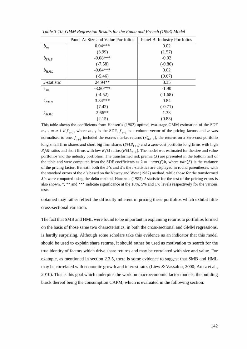
142

Table 3-10: GMM Regression Results for the Fama and French (1993) Model


𝑏𝑚 0.04***

(3.99)

0.02

(1.57)

𝑏𝑆𝑀𝐵 -0.08***

(-7.58)

-0.02

(-0.86)

𝑏𝐻𝑀𝐿 -0.04***

(-5.46)

0.02

(0.67)

J-statistic 24.94** 8.35

𝜆𝑚 -3.80***

(-4.52)

-1.90

(-1.68)

𝜆𝑆𝑀𝐵 3.34***

(7.42)

0.84

(-0.71)

𝜆𝐻𝑀𝐿 2.66**

(2.15)

1.33

(0.83)


𝑚𝑡+1 = 𝛼 + 𝑏′𝑓𝑡+1

, where 𝑚𝑡+1 is the SDF, 𝑓𝑡+1

is a column vector of the pricing factors and 𝛼 was

normalised to one. 𝑓𝑡+1

included the excess market returns (𝑟𝑚,𝑡+1𝑒 ), the returns on a zero-cost portfolio

long small firm shares and short big firm shares (𝑆𝑀𝐵𝑡+1) and a zero-cost portfolio long firms with high

𝐵/𝑀 ratios and short firms with low 𝐵/𝑀 ratios (𝐻𝑀𝐿𝑡+1). The model was estimated for the size and value

portfolios and the industry portfolios. The transformed risk premia (𝜆) are presented in the bottom half of

the table and were computed from the SDF coefficients as 𝜆 = −𝑣𝑎𝑟(𝑓)𝑏, where 𝑣𝑎𝑟(𝑓) is the variance

of the pricing factor. Beneath both the 𝑏’s and 𝜆’s the t-statistics are displayed in round parentheses, with

the standard errors of the 𝑏’s based on the Newey and West (1987) method, while those for the transformed

𝜆’s were computed using the delta method. Hansen’s (1982) J-statistic for the test of the pricing errors is

also shown. *, ** and *** indicate significance at the 10%, 5% and 1% levels respectively for the various

tests.

obtained may rather reflect the difficulty inherent in pricing these portfolios which exhibit little

cross-sectional variation.

The fact that SMB and HML were found to be important in explaining returns to portfolios formed

on the basis of those same two characteristics, in both the cross-sectional and GMM regressions,

is hardly surprising. Although some scholars take this evidence as an indicator that this model

should be used to explain share returns, it should rather be used as motivation to search for the

true identity of factors which drive share returns and may be correlated with size and value. For

example, as mentioned in section 2.3.5, there is some evidence to suggest that SMB and HML

may be correlated with economic growth and interest rates (Liew & Vassalou, 2000; Aretz et al.,

2010). This is this goal which underpins the work on macroeconomic factor models; the building

block thereof being the consumption CAPM, which is evaluated in the following section.

143

3.6.4 The Consumption CAPM


Prior to estimating the consumption CAPM the descriptive statistics of the consumption growth

rates were examined. As shown in Table 3-11, the average one-quarter consumption growth rate

was 0.52%, while that for the three-quarter horizon was much higher at 1.60%. The variation of

both measures (1.53% and 2.80% for the one-quarter and three-quarter growth rates respectively)

was substantially lower than that obtained for the average market returns of 9.74%; consistent

with the point highlighted by Cochrane (1996) that non-traded factors exhibit substantially less

variation and therefore their ability to capture time-series variation in returns is questionable.

There was evidence of mean reversion in the consumption growth series as reflected by the

negative first order autocorrelation, whereas the non-contemporaneous growth rate displayed

substantial positive autocorrelation, which is in keeping with the way the series was computed;

however, the series was still stationary based on both the ADF (at 10%) and KPSS tests.

Table 3-11: Descriptive Statistics of the Growth Rate in Consumption

∆𝑐𝑡+1 ∆𝑐𝑡+3

Avg. (%) 0.52 1.60

Std. Dev. (%) 1.53 2.80

𝜌(1) -0.07 0.68

ADF statistic -5.18*** -3.38*

KPSS statistic 0.05 0.05

This table shows the descriptive statistics of the one-period and three-period growth rates in consumption

(∆𝑐𝑡+1 and ∆𝑐𝑡+3 respectively) over the period July 1990 to April 2013. These include the average (avg.),

standard deviation (std. dev.), first-order autocorrelation (𝜌(1)), ADF and KPSS test statistics (using a trend

and intercept if appropriate). For the ADF test, the critical values from MacKinnon (1996) were used while

for the KPSS test, the Kwiatkowski et al. (1992) critical values were used. *, ** and *** indicate

significance at the 10%, 5% and 1% levels respectively for the ADF and KPSS tests.

The cross-sectional results for the consumption CAPM are displayed in Table 3-12. For the

canonical model the ��2 for the size and value portfolios was -5%, revealing that this model could

not explain any of the variation across the size- and value-sorted portfolios. This estimate was

lower than that for the CAPM documented in the preceding chapter. This finding that the overall

explanatory power of the consumption CAPM was worse than the CAPM is consistent with the

early test of Mankiw and Shapiro (1986) although more recent findings of Lettau and Ludvigson

(2001b) for the U.S and Li et al. (2011) for Australia found the opposite when examining size-

and value-sorted portfolios, albeit that the difference was small. As the results for both the AIC

and R2 in Table 3-12 indicate, measuring consumption growth over a longer horizon to account

for investor’s slow response to changes in consumption did not salvage the explanatory power of

the model. As explained in section 3.4.2, Li et al. (2011) documented a similar finding for the

Australian market but this differed from Parker and Julliard (2005) for the U.S, although the

144

Table 3-12: Cross-Sectional Regression Results for the Consumption CAPM


Consumption

CAPM

Non-

Contemporaneous

Consumption

CAPM

Consumption

CAPM

Non-

Contemporaneous

Consumption

CAPM

𝜆0 2.89

(2.94)***

{2.88}***

2.87

(2.80)***

{2.66}***

1.58

(4.23)***

{4.23}***

1.78

(4.39)***

{4.39}***

𝜆Δ𝑐𝑡+1 0.31

(1.91)*

{0.75}

-0.03

(-0.13)

{-0.05}

𝜆Δ𝑐𝑡+3 0.94

(2.31)**

{1.14}

-0.12

(-0.23)

{-0.11}

𝑅2

(��2)

0.02

(-0.05)

0.06

(-0.01)

0.53

(0.46)

0.62

(0.56)

AIC 1.51 1.51 -0.85 -1.35

Wald statistic 3.65*

{0.56}

5.33**

{1.31}

0.01

{0.00}

0.05

{0.01}

RMSE 1.82 1.82 0.72 0.62


{210.95}***

201.74***

{224.44}***

5.00

{6.29}

4.07

{6.01}


𝜆0 + 𝜆𝑓′𝛽𝑖𝑓

+ 𝜂𝑖, estimated over the period June 1990 to April 2013 across the 16 size and value portfolios

and nine industry portfolios, where 𝛽𝑖𝑓

is a column vector of the sensitivity of the portfolio returns to the

pricing factors (factor loadings) obtained from the time-series regressions. For the consumption CAPM, the

factor loading was the sensitivity to the growth rate in consumption (𝛽𝑖∆𝑐

), while for the non-

contemporaneous model, the factor loading was the sensitivity to the non-contemporaneous growth rate in

consumption (𝛽𝑖∆𝑐𝑡+3

). Beneath each coefficient in round parentheses is the t-statistic computed using the

Fama and MacBeth (1973) standard errors, while the second t-statistic in curly parentheses was calculated

using the Shanken (1992) standard errors. The Wald statistic provides a test of the joint significance of the



refers to the root mean squared pricing error across the portfolios. The 𝑅2 is Jagannathan and Wang’s (1996)

cross-sectional measure of explanatory power and ��2 is adjusted for the number of pricing factors. The AIC

refers to the Akaike information criteria and was computed similarly to Jagannathan and Wang’s (1996) 𝑅2.

*, ** and *** indicate significance at the 10%, 5% and 1% levels respectively for the various tests.

longer horizon over which consumption was measured in the latter study may account for the

differences observed. For the industry-sorted portfolios, the models performed substantially better

as they were able to explain 46% and 56% of the variation. Similarly to the CAPM and two-factor

models, the intercepts from both samples for the two consumption CAPM specifications were

positive and significant; again a finding consistent with international studies such as Lettau and

Ludvigson (2001b) and Li et al. (2011). Although these intercepts were much smaller than with

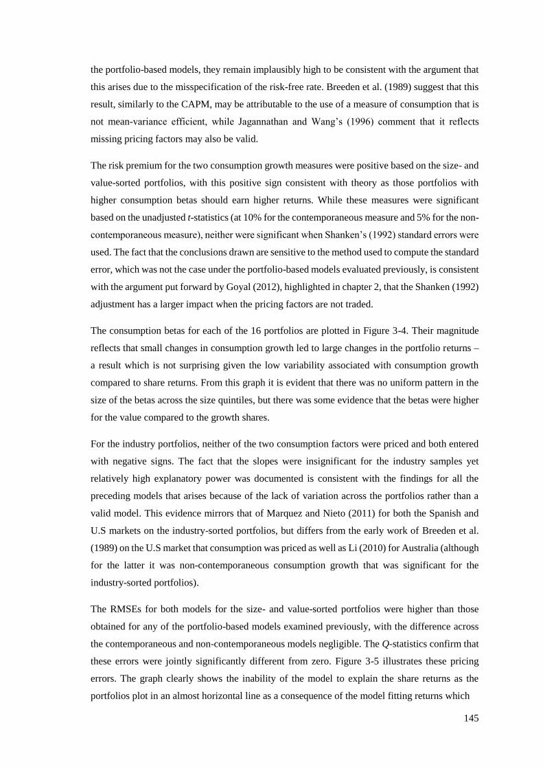
145

the portfolio-based models, they remain implausibly high to be consistent with the argument that

this arises due to the misspecification of the risk-free rate. Breeden et al. (1989) suggest that this

result, similarly to the CAPM, may be attributable to the use of a measure of consumption that is

not mean-variance efficient, while Jagannathan and Wang’s (1996) comment that it reflects

missing pricing factors may also be valid.

The risk premium for the two consumption growth measures were positive based on the size- and

value-sorted portfolios, with this positive sign consistent with theory as those portfolios with

higher consumption betas should earn higher returns. While these measures were significant

based on the unadjusted t-statistics (at 10% for the contemporaneous measure and 5% for the non-

contemporaneous measure), neither were significant when Shanken’s (1992) standard errors were

used. The fact that the conclusions drawn are sensitive to the method used to compute the standard

error, which was not the case under the portfolio-based models evaluated previously, is consistent

with the argument put forward by Goyal (2012), highlighted in chapter 2, that the Shanken (1992)

adjustment has a larger impact when the pricing factors are not traded.

The consumption betas for each of the 16 portfolios are plotted in Figure 3-4. Their magnitude

reflects that small changes in consumption growth led to large changes in the portfolio returns –

a result which is not surprising given the low variability associated with consumption growth

compared to share returns. From this graph it is evident that there was no uniform pattern in the

size of the betas across the size quintiles, but there was some evidence that the betas were higher

for the value compared to the growth shares.

For the industry portfolios, neither of the two consumption factors were priced and both entered

with negative signs. The fact that the slopes were insignificant for the industry samples yet

relatively high explanatory power was documented is consistent with the findings for all the

preceding models that arises because of the lack of variation across the portfolios rather than a

valid model. This evidence mirrors that of Marquez and Nieto (2011) for both the Spanish and

U.S markets on the industry-sorted portfolios, but differs from the early work of Breeden et al.

(1989) on the U.S market that consumption was priced as well as Li (2010) for Australia (although

for the latter it was non-contemporaneous consumption growth that was significant for the

industry-sorted portfolios).

The RMSEs for both models for the size- and value-sorted portfolios were higher than those

obtained for any of the portfolio-based models examined previously, with the difference across

the contemporaneous and non-contemporaneous models negligible. The Q-statistics confirm that

these errors were jointly significantly different from zero. Figure 3-5 illustrates these pricing

errors. The graph clearly shows the inability of the model to explain the share returns as the

portfolios plot in an almost horizontal line as a consequence of the model fitting returns which

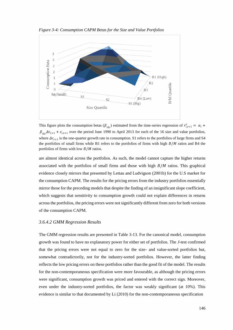
146

Figure 3-4: Consumption CAPM Betas for the Size and Value Portfolios

This figure plots the consumption betas (𝛽𝑖∆𝑐

) estimated from the time-series regression of 𝑟𝑖,𝑡+1𝑒 = 𝛼𝑖 +

𝛽𝑖∆𝑐

𝛥𝑐𝑡+1 + 휀𝑖,𝑡+1 over the period June 1990 to April 2013 for each of the 16 size and value portfolios,

where 𝛥𝑐𝑡+1 is the one-quarter growth rate in consumption. S1 refers to the portfolios of large firms and S4



are almost identical across the portfolios. As such, the model cannot capture the higher returns

associated with the portfolios of small firms and those with high 𝐵/𝑀 ratios. This graphical

evidence closely mirrors that presented by Lettau and Ludvigson (2001b) for the U.S market for

the consumption CAPM. The results for the pricing errors from the industry portfolios essentially

mirror those for the preceding models that despite the finding of an insignificant slope coefficient,

which suggests that sensitivity to consumption growth could not explain differences in returns

across the portfolios, the pricing errors were not significantly different from zero for both versions

of the consumption CAPM.


The GMM regression results are presented in Table 3-13. For the canonical model, consumption

growth was found to have no explanatory power for either set of portfolios. The J-test confirmed

that the pricing errors were not equal to zero for the size- and value-sorted portfolios but,

somewhat contradictorily, not for the industry-sorted portfolios. However, the latter finding

reflects the low pricing errors on these portfolios rather than the good fit of the model. The results

for the non-contemporaneous specification were more favourable, as although the pricing errors

were significant, consumption growth was priced and entered with the correct sign. Moreover,

even under the industry-sorted portfolios, the factor was weakly significant (at 10%). This

evidence is similar to that documented by Li (2010) for the non-contemporaneous specification

147

Figure 3-5: Pricing Errors from the Consumption CAPM for the Size and Value Portfolios


𝑒 = 𝜆0 + 𝜆Δ𝑐𝛽iΔ𝑐

+ 𝜂𝑖 over the

period June 1990 to April 2013 across the 16 size and value portfolios, where 𝛽iΔ𝑐

measures the sensitivity

of the portfolio returns to the one-quarter growth rate in consumption. S1 refers to the portfolios of large

firms and S4 the portfolios of small firms while B1 refers to the portfolios of firms with high 𝐵/𝑀 ratios

and B4 the portfolios of firms with low 𝐵/𝑀 ratios.

on the Australian market when estimated via maximum-likelihood (which was not true when the

cross-sectional OLS approach was used in the study of Li et al., 2011) and thus the differences in

the results observed do reflect the varying estimation methods. Thus, the finding of some role for

consumption growth in the pricing of securities on the JSE is consistent with the more general

view of Faff and Olivier (1998) that relationships between macroeconomic variables and stock

markets may take time to emerge and that of Parker and Julliard (2005) with specific reference to

consumption growth.

As noted previously, the generally poor performance of the consumption CAPM internationally

has been attributed to the low participation rates of consumers in the share market. The same is

arguable true, and potentially even more pronounced, in an emerging market like South Africa

with very high poverty levels and low savings rates and thus may explain the results which largely

point to a very limited role for consumption in the pricing of securities. However, the results may

also speak to the fact that the measure of consumption does not encapsulate all risk and thus,

models which have sought to expand the measure of consumption are considered further in the

following chapters.

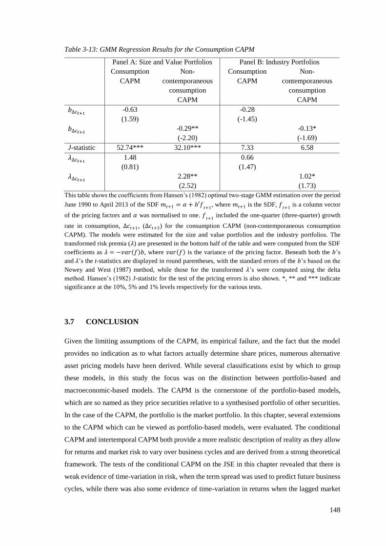
148

Table 3-13: GMM Regression Results for the Consumption CAPM


Consumption

CAPM

Non-

contemporaneous

consumption

CAPM

Consumption

CAPM

Non-

contemporaneous

consumption

CAPM

𝑏∆𝑐𝑡+1 -0.63

(1.59)

-0.28

(-1.45)

𝑏∆𝑐𝑡+3 -0.29**

(-2.20)

-0.13*

(-1.69)

J-statistic 52.74*** 32.10*** 7.33 6.58

𝜆∆𝑐𝑡+1 1.48

(0.81)

0.66

(1.47)

𝜆∆𝑐𝑡+3 2.28**

(2.52)

1.02*

(1.73)

This table shows the coefficients from Hansen’s (1982) optimal two-stage GMM estimation over the period

June 1990 to April 2013 of the SDF 𝑚𝑡+1 = 𝛼 + 𝑏′𝑓𝑡+1

, where 𝑚𝑡+1 is the SDF, 𝑓𝑡+1

is a column vector

of the pricing factors and 𝛼 was normalised to one. 𝑓𝑡+1

included the one-quarter (three-quarter) growth

rate in consumption, ∆𝑐𝑡+1, (∆𝑐𝑡+3) for the consumption CAPM (non-contemporaneous consumption

CAPM). The models were estimated for the size and value portfolios and the industry portfolios. The

transformed risk premia (𝜆) are presented in the bottom half of the table and were computed from the SDF

coefficients as 𝜆 = −𝑣𝑎𝑟(𝑓)𝑏, where 𝑣𝑎𝑟(𝑓) is the variance of the pricing factor. Beneath both the 𝑏’s

and 𝜆’s the t-statistics are displayed in round parentheses, with the standard errors of the 𝑏’s based on the

Newey and West (1987) method, while those for the transformed 𝜆’s were computed using the delta

method. Hansen’s (1982) J-statistic for the test of the pricing errors is also shown. *, ** and *** indicate

significance at the 10%, 5% and 1% levels respectively for the various tests.

3.7 CONCLUSION

Given the limiting assumptions of the CAPM, its empirical failure, and the fact that the model

provides no indication as to what factors actually determine share prices, numerous alternative

asset pricing models have been derived. While several classifications exist by which to group

these models, in this study the focus was on the distinction between portfolio-based and

macroeconomic-based models. The CAPM is the cornerstone of the portfolio-based models,

which are so named as they price securities relative to a synthesised portfolio of other securities.

In the case of the CAPM, the portfolio is the market portfolio. In this chapter, several extensions

to the CAPM which can be viewed as portfolio-based models, were evaluated. The conditional

CAPM and intertemporal CAPM both provide a more realistic description of reality as they allow

for returns and market risk to vary over business cycles and are derived from a strong theoretical

framework. The tests of the conditional CAPM on the JSE in this chapter revealed that there is

weak evidence of time-variation in risk, when the term spread was used to predict future business

cycles, while there was also some evidence of time-variation in returns when the lagged market

149

risk premium was used as the conditioning variable. However, the market risk premium remained

significant and negative in contrast to theory and the pricing errors of the model were significant

such that the models could not adequately explain the size and value anomalies.

Fama and French’s (1993) three-factor model, also a portfolio-based model, was seen to be

entirely empirically motivated with the two additional pricing factors – SMB and HML – having

little theoretical underpinning. However, similarly to international studies, the results of this study

found that the model was able to explain a substantial portion of the cross-sectional variation of

the size and value portfolios on the JSE, with an ��2 of 70%; although the pricing errors were still

significant based on the adjusted test statistic.

While some of these models may be theoretically appealing and/or perform well, none are able to

provide insight as to the fundamental determinants of share returns. This is the central concern of

macroeconomic-based asset pricing. The consumption CAPM is the key building block for these

models as it links the macroeconomy to share returns through the utility individuals derive from

consumption. This model was tested on the JSE and found to perform as poorly, if not worse, than

the CAPM with a negative ��2. Thus, although there was weak evidence that consumption growth

was priced in the cross-section this factor could not explain the differences in returns across

portfolios sorted based on size and value or industry affiliation. This evidence is not, however,

unique to the emerging South African market as similar evidence has been documented on

international markets such as the U.S and Australia. One possible explanation for the poor

performance of the model is that because aggregate consumption cannot be directly observed, the

proxies used may be inadequate and thus not fully capture all risk inherent in consumption

decisions. This line of thinking has spurred considerable research as scholars examine the impact

of other factors on consumption. Most notable in this regard are labour income and housing wealth

which are considered in chapters 4 and 5.

150

Chapter 4 : THE ROLE OF LABOUR INCOME IN ASSET PRICING

4.1 INTRODUCTION

As mentioned in section 3.4, understanding and measuring the macroeconomic risks that drive

asset prices is critical. Considerable research has focused on this issue, spurred in particular by

the attempts to link the size and value factors of Fama and French (1993) to observable risk.

Various macroeconomic variables have been reviewed but in this chapter and chapter 5 the focus

is on human capital (measured by labour income) and housing wealth. Inflation or industrial

production, for example, may influence returns, but this provides the answer to the wrong

question. That is, the question is not whether the selected variables affect returns (as per APT)

but whether they affect the behaviour of investors in their demand for securities. Hence at an

aggregate level these factors may be important but individual investors are more likely to be

concerned about how their labour income or housing wealth moves with share returns.

Accordingly, much of this discussion centres around how the variables in question affect

consumption through the consumption CAPM.

The ability of an investor to consume goods and services is directly tied to their labour income,

as if an individual is likely to lose their job in the future, their consumption will change (Cochrane,

2008a). This will impact on security prices as those investments which pay out when labour

income is low will provide greater marginal utility than those investments which yield high

returns when labour income is high (Fama & French, 2004). This linkage between consumption,

labour income and financial returns has been confirmed by Lettau and Ludvigson (2001a) and

Santos and Veronesi (2006).

The measures of consumption usually used in tests of the consumption CAPM are proxies as

aggregate consumption is not observable. However, these proxies may not accurately capture the

relationship between consumption and labour income. Moreover, the model itself has been

criticised because it does not allow for variation in risk and return over time. Accordingly, the

consumption CAPM has been extended to not only capture the influence of labour income on the

returns of securities through the interaction with consumption but also to allow for time-variation

in the risk measures.

The study of the role of labour income on asset prices originated in the CAPM framework as a

means to provide a more encompassing estimate of the market portfolio rather than that based

solely on the returns from ordinary shares. Studies such as Jagannathan and Wang (1996),

Campbell (1996) and Jagannathan et al. (1998) thus do not directly consider the link between

151

consumption, labour income and share returns, but they do still provide important information

regarding labour income as a risk factor. In this regard, the evidence is somewhat mixed as to

whether the sensitivity of security returns to labour income is priced in the cross-section of share

returns.

The goal of the analysis in this chapter is to ascertain whether these models that include labour

income, either directly in the pricing equation or through the linkage to consumption, can explain

differences in returns across shares listed on the JSE. The remainder of the chapter is laid out as

follows: the difficulties in measuring human capital are reviewed, followed by a discussion of the

models that have been derived to account for labour income in asset pricing and a critique of their

performance. Thereafter, several of these models are tested on the JSE and the results compared

both to the international literature and the success of the other asset pricing specifications tested

in chapters 2 and 3.

4.2 LABOUR INCOME IN ASSET PRICING

4.2.1 The Importance of Human Capital

The ability of an individual to consume goods and services in the current and following periods

is affected by human capital (Mayers, 1973). Consumption patterns will thus vary over time in

response to variations in human capital. This in turn will affect asset prices, because if a security

pays out when returns to human capital are low, the security will provide greater marginal utility

than a security which pays out when returns to human capital are high. For example, individuals

will avoid investing in shares which are likely to perform poorly in conditions when there is

substantial risk of them losing their job (Cochrane, 2008a, pp. 302). Accordingly, there is a

theoretical linkage between consumption, labour income and share returns. Lettau and Ludvigson

(2001a) and Santos and Veronesi (2006) derived measures to examine the relationship between

consumption and labour income in different stages of the business cycle and showed that these

measures are linked to share market returns. In fact, these ratios could explain future returns

because of their variation across business cycles.

Under the consumption CAPM, security prices are assumed to be influenced only by the

consumption of non-durable goods and services and not directly by other potential sources of

utility. Accordingly, any risk associated with human capital should be fully incorporated into the

consumption measure.53 However, not only are the measures used for consumption proxies, but

53 Human capital is assumed to provide utility to an individual through consumption and leisure. Given that

under the consumption CAPM, the representative agent’s utility is measured only over consumption of non-

152

they are also subject to numerous measurement problems, as discussed in section 3.4.2. These

include their focus on expenditure rather than consumption, sampling error and capturing

household consumption as the residual after government and business expenditure. Moreover, the

model has also been criticised because consumption varies very little compared to fluctuations in

the share market which it seeks to explain, while consumption is also measured at an aggregate

level which may not be appropriate because not all consumers are investors. In light of these

problems, the argument has been made that the consumption CAPM may not accurately capture

the risk-return dynamics in the market (Cochrane, 2008a, pp. 302) and, in particular, may not

adequately capture the risk associated with human capital. Given the link between consumption,

labour income and share returns and the success of the composite variables of Lettau and

Ludvigson (2001a) and Santos and Veronesi (2006) in explaining future returns, these ratios have

been proposed as conditioning variables in asset pricing models. In so doing, these ratios can be

used to capture varying risk and return which static models do not allow for, but also incorporate

the consumption risk arising from human capital.

As highlighted in section 2.3.3, Roll (1977) argued that measuring the returns on the market

portfolio in the CAPM using an ordinary share index is inappropriate as it only captures financial

wealth and thus ignores all other components of wealth. Human capital has been shown to be the

largest constituent of the total wealth portfolio in both the U.S (Campbell, 1996; Jagannathan &

Wang, 1996; Zhang, 2006) and Japan (Jagnnathan et al., 1998) and thus investors are likely to be

concerned about how their labour income fluctuates with share returns (Fama & French, 2004).

The inclusion of human capital alongside financial wealth goes some way to providing a more

accurate measure of the total wealth portfolio (Jagannathan & Wang, 1996; Lustig & van

Nieuwerburgh, 2008; Bansal et al., 2014). Thus, several of the initial studies into the effects of

human capital on asset pricing are derived in the context of the CAPM so as to determine whether

the poor performance of the CAPM in empirical tests can be attributed to this use of an

inappropriate market portfolio proxy (Fama & French, 2004). These studies therefore provide

important information about how labour income affects asset prices. Although they do not directly

examine links between consumption, labour income and returns, an indirect link is still considered

as total wealth is the major determinant of consumption (Cochrane, 2008a). Moreover, as

mentioned in section 3.4.1, the extent of this can be seen in that many researchers focus on total

wealth in their models rather than aggregate consumption because the latter is not directly

durable goods and services as it is separate from other sources of utility, any utility from leisure derived

from human capital does not affect the pricing of securities. More recent studies have expanded the

possibility that the utility from consumption and leisure are not separable (such as Favilukus & Lin, 2013;

Dittmar et al., 2015) and the impact thereof on the pricing equation. Such research falls beyond the scope

of this study.

153

observable (see for example Santos & Veronesi, 2006; Lustig & van Nieuwerburgh, 2008).

Accordingly, these initial studies of the role of human capital in pricing securities are reviewed

in this chapter. Prior to this, however, it was necessary to consider the measurement of human

capital and the implications thereof for the asset pricing tests and thus this is reviewed in the

following sub-section.

4.2.2 Measuring Human Capital

The measurement of human capital complicates the ability of scholars to include this factor into

asset pricing models. Mayers (1972) maintained that almost all investors have a substantial

holding of non-marketable human capital, most notably claims to future labour income, social

security payouts or those from a private retirement fund. The model developed by Mayers (1972)

to include human capital was thus founded on the non-marketable nature of this asset. In the tests

of this model by Fama and Schwert (1977) labour income was used as a proxy for human capital.

Jagannathan and Wang (1996) disputed the view that human capital is not tradeable arguing that

insurance markets, such as life assurance, medical aid, and disability insurance, allow individuals

to hedge their human capital risk, while mortgage bonds essentially represent borrowing against

expected future income. Accordingly, Jagannathan and Wang (1996) proposed that human capital

should be viewed in the same manner as any other tradable asset. The major component of human

capital is labour income and thus Jagannathan and Wang (1996) argued that a measure of the

latter should provide a good approximation of human capital. However, it is not possible to

measure the returns to labour income by examining the returns on mortgage-backed securities, as

not all labour income is used to pay these liabilities. Instead, Jagannathan and Wang (1996)

proposed using the growth rate in aggregate labour income as the measure. Interestingly, this was

the same proxy as used by Fama and Schwert (1977) in the testing of the model of Mayers (1972)

where human capital was viewed as non-marketable. Further research such as Hodrick and Zhang

(2001), Lettau and Ludvigson (2001b), Santos and Veronesi (2006) and Lustig and van

Nieuwerburgh (2005, 2008) have used this same measure.

Campbell (1996) also measured the returns to human capital as the returns on labour income.

However, rather than viewing labour income as a proxy for human capital, he deemed it as a

dividend of human capital. Accordingly, he argued that it was necessary to account for the

expected future growth rate in labour income as is done when using dividend payments to value

a share in the dividend discount model (as per that presented in chapter 3). Thus, his measure of

the growth rate in human capital comprised the growth in labour income and a prediction of the

expected future growth rate in labour income.

154

Palacios-Huerta (2003), however, criticised both of these measures arguing that the reliance on

labour income ignores important components of human capital such as capital gains associated

with the stock of human capital, that labour supply is endogenous, the role of worker experience,

the possibility of premiums associated with specific skills, the effect of physical capital on labour

income and the growth rate in labour income. These factors were included in a composite measure

of aggregate human capital by weighting the various components based on factors such as gender,

education and experience. Eiling (2013) also recognised that aggregate labour income may be a

poor measure of human capital as it is likely to be affected by age, education or even the industry

in which the investor is employed. Similarly to Mayers (1972), Eiling (2013) contended that

human capital should be viewed as a non-tradeable asset as although investors may borrow against

future labour income, the majority would be unlikely to trade claims against this income due to

adverse selection and moral hazard problems.54 Thus, rather than devising an aggregate measure

from disaggregated data as per Palacios-Huerta (2003), Eiling (2013) modelled human capital as

heterogeneous but with the industry affiliations of firms providing homogeneity. However, the

implementation of human capital as non-tradeable complicates asset pricing specifications, with

more recent studies by Bansal et al. (2014) and Dittmar et al. (2015) also continuing to favour the

use of aggregate growth in labour income for measuring human capital. Accordingly, in this study,

the focus is on labour income which is used as a measure of human capital.

4.2.3 Asset Pricing Models with Labour Income

As mentioned, Mayers (1972) was the first to recognise the need to incorporate human capital

into the CAPM. Due to the non-tradeable nature of human capital in his model, the specification

proved difficult to test, as it allows for individuals to hold different combinations of portfolios

based on their need to hedge their occupational risks (as opposed to the CAPM where all investors

hold the same two funds – the risk-free rate and market portfolio). However, Fama and Schwert

(1977) did test the model using a measure of aggregate labour income and found that Mayers’s

(1972) model had little ability to explain returns.

Jagannathan and Wang (1996) assumed that the returns to the market portfolio are a linear

function of the returns to the value-weighted share index and the returns to the growth rate in total

labour income. This yields a two-factor model as follows

𝐸(��𝑖,𝑡+1𝑒 ) = 𝜆0 + 𝜆𝑚𝛽𝑖𝑚 + 𝜆Δ𝑦𝛽Δ𝑦, (4.1)

54 Adverse selection refers to the possibility that those individuals exposed to greater human capital risk

will be more likely to purchase insurance than those with lower human capital risk, while moral hazard

refers to the possibility that an individual may change their behaviour because they have insurance against

future labour income.

155

where Δ𝑦 measures the growth rate in labour income and 𝛽𝑦𝑡 is the labour beta which captures

the sensitivity of security returns to labour income growth (Jagannathan & Wang, 1996, p. 15).

This labour beta was estimated similarly to other factor loadings via a time-series regression of

the portfolio returns against the growth rate in labour income. Jagannathan and Wang (1996, p.

15) extended this expansion of the market portfolio to include their time-varying risk measure (as

per equation 3.16) which gave rise a three-factor model as follows

𝐸(��𝑖,𝑡+1𝑒 ) = 𝜆0 + 𝜆𝑚𝛽𝑖𝑚 + 𝜆𝑧𝛽𝑖𝑧 + 𝜆Δ𝑦𝛽Δ𝑦. (4.2)

Jagannathan and Wang (1996) found that the CAPM with labour income (4.1) was able to explain

30% of the variation in returns across size- and beta-sorted portfolios, which represented a

substantial improvement on the 1% of the CAPM. The labour risk premium was positive and

significant signalling that those securities which had a higher correlation with the returns to labour

income required higher returns to compensate investors for the fact that these securities paid out

when labour income was already high. However, as per the CAPM, the estimate of the market

risk premium was insignificant. When the labour beta was included in the conditional CAPM, the

��2 increased to 55%, with the labour risk premium positive and significant. This ��2 was almost

equivalent to that obtained for the Fama and French (1993) three-factor model by Jagannathan

and Wang (1996) for their size- and beta-sorted portfolios. When size and the 𝐵/𝑀 ratio were

included as additional pricing factors in the conditional CAPM with labour income they were not

significant. Jagannathan and Wang (1996) thus suggested that size and value may proxy for the

risk associated with time-variation in beta and labour income in pricing securities. Further tests

by Jagannathan and Wang (1996) revealed that labour income and variability in beta did not proxy

for other macroeconomic variables and in addition, provided greater explanatory power than the

APT using the four macroeconomic variables of Chen et al. (1986).

Palacios-Huerta (2003) noted that the explanatory power of the CAPM with labour income

improved substantially when their expanded measure of human capital was employed, with the

most important component of human capital being the risks associated with capital gains and skill

premia. But, similarly to Jagannathan and Wang (1996), Palacios-Huerta (2003) found that

including a measure of human capital was not sufficient to resurrect the CAPM, as allowing for

time-variation in beta estimates was also necessary.

Consistent with the link between the expected return-beta framework and a linear SDF proposed

by Dybvig and Ingersoll (1982), Lettau and Ludvigson (2001b) specified the linear SDF implied

by the CAPM with labour income of 4.1 as follows

𝑚𝑡+1 = 𝛼0 + 𝑏0𝑟𝑚,𝑡+1𝑒 + 𝑏1Δ𝑦𝑡+1. (4.3)

156

In an examination of the 25 size- and value-sorted portfolios on the U.S market, they obtained

similar results to Jagannathan and Wang (1996) in that the labour risk premium was identified to

be positive and significant, while the market risk premium was insignificant. Lettau and

Ludvigson (2001b) also noted a substantial improvement in ��2 from -0.03% for the CAPM to

54% for the CAPM with labour income. Comparing the explanatory power across the studies of

Jagannathan and Wang (1996) and Lettau and Ludvigson (2001b) suggests that the CAPM with

labour income performed better in explaining patterns across portfolios formed on the basis of

size and value than size and betas; however, Lettau and Ludvigson (2001b) did not conduct any

further tests of the CAPM with labour income to ascertain whether the model was better able to

explain the premia associated with small or value shares. The conditional CAPM with labour

income of Lettau and Ludvigson (2001b) yielded an even higher measure of explanatory power

but this increase over the CAPM with labour income was predominantly due to their choice of

conditioning variable. Labour income is a crucial measure in the explanatory variable derived by

Lettau and Ludvigson (2001b) and is thus analysed in more detail in the following section.

The findings of Santos and Veronesi (2006) contrast with those of Jagannathan and Wang (1996)

and Lettau and Ludvigson (2001b), as in their test of the CAPM with labour income in the U.S,

they found that the labour risk premium was insignificant, with the ��2 lower than that of the

CAPM (0.4% compared to 4%). Santos and Veronesi (2006) did use a longer period (1948 to

2001) compared to the other two studies (1963 to 1998) while they also did not follow the timing

convention of Jagannathan and Wang (1996) (which Lettau & Ludvigson, 2001b did) of lagging

labour income by one month to account for the delay in investor’s obtaining this information. To

assess the impact of these differences in the sample and method on their results, Santos and

Veronesi (2006) re-estimated the CAPM with labour income using the lagged value of labour

income growth over their whole period and the shorter period used in the previous studies. They

found that the use of the lagged value did result in a significant labour risk premium but only for

the shorter sample period. Accordingly, their analysis revealed that the finding that labour income

was a priced factor in returns was germane only to a relatively short horizon in the U.S and was

sensitive to the timing of the labour income measure. The results of Hodrick and Zhang’s (2001)

test of the conditional CAPM with labour income validate Santos and Veronesi’s (2006)

assertions, as over the period 1953 to 1997, they found that the labour beta was not priced in the

cross-section even when following the measurement convention of Jagannathan and Wang

(1996). However, Hodrick and Zhang (2001) did find some support for the existence of a time-

varying component to the labour beta.

Alongside the early work of Mayers (1972) and Jagannathan and Wang (1996), the paper of

Campbell (1996) also made a notable contribution on the role of labour income in asset pricing.

Campbell (1996) utilised the intertemporal framework as the basis for his model. As indicated in

157

equation 3.6 (𝐸(𝑟𝑖,𝑡+1𝑒 ) = 𝛾𝑖𝑚𝑐𝑜𝑣(𝑟𝑖,𝑡+1, 𝑟𝑚,𝑡+1) + 𝛾𝑖𝑧′𝑐𝑜𝑣(𝑟𝑖,𝑡+1, Δ𝑧𝑡+1)), the intertemporal

CAPM shows that the expected return on a security depends on two factors - the covariance

between the security and market returns (similarly to the CAPM) and the covariance between the

security returns and innovations in the state variables. The state variables are those which are able

to explain future share returns and capture how investors hedge against adverse market

movements in the future. Campbell (1996) maintained that future labour income is of importance

to investors as this will affect their ability to consume in the future. Consequently, he proposed

that they will try to hedge against adverse movements in labour income similarly to adverse

movements in the market. Accordingly, Campbell (1996) extended the intertemporal model to

incorporate a term to capture this hedging against labour income risk, with the model as follows

𝐸(𝑟𝑖,𝑡+1𝑒 ) = 𝛾𝑖𝑚𝑐𝑜𝑣(𝑟𝑖,𝑡+1, 𝑟𝑚,𝑡+1) + 𝛾𝑖𝑧 ′𝑐𝑜𝑣(𝑟𝑖,𝑡+1, Δ𝑧𝑡+1) + 𝛾𝑖𝑥 ′𝑐𝑜𝑣(𝑟𝑖,𝑡+1, Δ𝑥𝑡+1)

(4.4)

where Δ𝑥𝑡+1 is the innovation in the variables 𝑥𝑡 that can explain growth in labour income

(Campbell, 1996, p. 309). If investors wish to hedge against future changes in labour income, then

they must be able to explain future labour income. Using the same set of variables as used to

examine the predictability of share returns, Campbell (1996) found that the growth rate in labour

income could be forecasted using the term spread and growth in gross national product. The term

spread was also able to explain future share returns along with the relative T-bill yield and 𝐷/𝑃

ratio.

Campbell (1996) found evidence of a positive risk-return relationship as the covariance of the

portfolio and market returns was highest for those portfolios with the highest average returns for

both the industry- and size-sorted portfolios. In addition, the estimates of the covariances of the

portfolios returns with news about future returns were significant and negative, with the negative

coefficients demonstrating evidence of mean reversion in returns (a positive value of the index

return in the current period was associated with lower expectations of future returns) (Campbell,

1996). The news about labour income growth was found to be positive but insignificant in all

permutations; showing very little role for labour income in the pricing of securities in the

intertemporal framework. However, Campbell’s (1996) tests provided no insight into the value

anomaly because the portfolios were sorted based on size and industry.

Out of sample evidence of the importance of labour income in explaining the returns on size- and

value-sorted portfolio was documented by Jagnnathan et al. (1998) for Japan. They found that the

inclusion of labour income in the CAPM increased the ��2 from 2% to 75%, showing that in the

Japanese market, labour income was even more important in explaining returns than in the U.S.

However, the market risk premium remained insignificant. Further analysis revealed that the

inclusion of labour income was largely able to account for the size effect as the premium

158

associated with small shares could be viewed as compensation for holding shares which moved

closely with labour income while larger shares did not require this premium because they were

not highly correlated with growth in labour income (and effectively represented a hedge against

labour income). However, labour income had little explanatory power for the value premium. Li

et al. (2011), in contrast, found that while labour income was priced for Australian share returns,

it entered with a surprising negative sign and also had little ability to explain the cross-section of

share returns as a negative ��2 was obtained.

Overall, the results of tests of the models augmented with human capital are mixed as they suggest

that the importance of labour income differs across countries and over time. Moreover, the fact

that the inclusion of labour income does not salvage the market risk-return relationship

undermines the theoretical basis on which this specification is built in the framework of the

CAPM. That is, if the CAPM is valid but the empirical shortcomings arise due to the use of an

inappropriate measure of the market portfolio, then the market risk premium should be positive

and significant when the growth rate in labour income is included so as to account for this

shortcoming, which it is not. The same reasoning is also true for when the total wealth portfolio

is used as a proxy for aggregate consumption. The fact that labour income does not necessarily

affect share returns in aggregate does not necessarily mean that this macroeconomic factor does

not play a fundamental role in the demand for securities by investors through its impact on

consumption. As mentioned in section 4.1, there is evidence to suggest that the interaction

between labour income and consumption can forecast future returns due to the changing nature

of the relationship between the two variables in different stages of the business cycles. This

forecasting power of the consumption and labour income composite variables has important

implications for asset pricing where variation in risk and return are associated with fluctuations

in the business cycle. These issues are considered in the following section.

4.2.4 Conditional Models with Scaling Factors that Include Labour Income

4.2.4.1 Lettau and Ludvigson (2001b)

The consumption CAPM shows how an investor’s goal to maximise lifetime consumption

influences their demand for securities. Allied to this, as has been discussed above, the ability of

an investor to consume and invest is also affected by their labour income. In light of the

interconnectedness between consumption, labour income and asset wealth, Lettau and Ludvigson

(2001a) devised a unique composite variable which captures the interaction between these three

variables. The derivation thereof is outlined below.

The standard intertemporal budget constraint of investors for 𝑡 = 1, 2 … 𝑇 is as follows

𝑊𝑡+1 = 𝑅𝑤𝑡(𝑊𝑡 − 𝐶𝑡), (4.5)

159

where 𝑊𝑡 is total wealth, 𝑅𝑤𝑡 is the gross return to total wealth (consistent with the definition in

chapter 2 that 𝑅𝑤𝑡 = 1 + 𝑟𝑤𝑡) and 𝐶𝑡 is consumption (Campbell & Mankiw, 1989, p. 204). This

budget constraint demonstrates that an investor’s total wealth in the following period is

determined by the total wealth invested in the current period (i.e. that which is not consumed)

grown by the total returns from investing the funds. By introducing logs and obtaining a first-

order Taylor series expansion of 4.5 to impose linearity yields

∆𝑤𝑡+1 ≈ (𝑟𝑤𝑡+1) + (1 −1

𝑝𝑤)(𝑐𝑡 − 𝑤𝑡), (4.6)

where ∆𝑤𝑡+1 is the change in the log of wealth, 𝑝𝑤 is the steady-state ratio of invested to total

wealth (𝑊𝑡 − 𝐶𝑡)/𝑊𝑡 and all variables in small letters refer to logged values (Campbell &

Mankiw, 1989, p. 204). By solving this difference equation forward, taking expectations and

imposing a transversality condition ( lim𝑖→∞

𝑝𝑤𝑖 (𝑐𝑡+𝑖 − 𝑤𝑡+𝑖) = 0), Campbell and Mankiw (1989, p.

204) derived a formulation for the log consumption-wealth ratio (𝑐𝑡 − 𝑤𝑡) as55

(𝑐𝑡 − 𝑤𝑡) ≈ 𝐸 ∑ 𝑝𝑤𝑖∞

𝑖=1 (𝑟𝑤𝑡+1 − ∆𝑐𝑡+1). (4.7)

Assuming that the returns to total wealth and the consumption growth rate are stationary on the

right-hand side of 4.7, this equation implies that consumption and wealth, the two non-stationary

variables on the left-hand side of 4.7, must be cointegrated (Lettau & Ludvigson, 2010). This is

similar to the argument presented in explaining share returns using 𝐷/𝑃 in section 3.2.1.3 that

dividends and prices must be cointegrated. Drawing from Granger’s (1986) representation

theorem, equation 4.7 also reveals that any deviations in the long-run relationship between

consumption and wealth in the current period will lead to changes in the returns to total wealth or

consumption growth in the following period. Thus, the consumption-wealth ratio should be able

to explain future values of either the returns to wealth or the consumption growth rate (Lettau &

Ludvigson, 2001a, pp. 820).

The limitation with this specification of the consumption-wealth ratio by Campbell and Mankiw

(1989) is that aggregate wealth is not directly observable. To overcome this limitation, Lettau and

Ludvigson (2001a, pp. 820) decomposed total wealth into asset (𝐴𝑡) and human capital (𝐻𝑡)

wealth such that 𝑊𝑡 = 𝐴𝑡 + 𝐻𝑡, with log aggregate wealth approximated as 𝑤𝑡 ≈ 𝜔𝑎𝑡 + (1 −

𝜔)ℎ𝑡, where 𝜔 represents the share of asset wealth in total wealth (𝐴𝑡/𝑊𝑡). The returns to

aggregate wealth can be decomposed into the return on its two components

𝑅𝑤𝑡 = 𝜔𝑅𝑎𝑡 + (1 − 𝜔)𝑅ℎ𝑡, (4.8)

55 The constant in this equation is excluded from the derivation as it simplifies the analysis.

160

and following Campbell (1996), this can be rewritten into an equation for log returns

𝑟𝑤𝑡 ≈ 𝜔𝑟𝑎𝑡 + (1 − 𝜔)𝑟ℎ𝑡. (4.9)

Substituting 𝑤𝑡 ≈ 𝜔𝑎𝑡 + (1 − 𝜔)ℎ𝑡 into the left-hand side of equation 4.7 and 4.9 into the right-

hand side of 4.7 yields the following specification

𝑐𝑡 − 𝜔𝑎𝑡 − (1 − 𝜔)ℎ𝑡 = 𝐸 ∑ 𝑝𝑤𝑖∞

𝑖=1 (𝜔𝑟𝑎𝑡 + (1 − 𝜔)𝑟ℎ𝑡 − ∆𝑐𝑡+1). (4.10)

Drawing on Jagannathan and Wang’s (1996) assertion that human capital is marketable, Lettau

and Ludvigson (2001a, pp. 820) assumed that human capital is a function of labour income such

that ℎ𝑡 = 𝜅 + 𝑦𝑡 + 𝑧𝑡, where 𝑦𝑡 is the log of labour income and 𝑧𝑡 is assumed to be a zero mean

stochastic stationary variable. Substituting this into 4.10 (ignoring the constant) yields

𝑐𝑡 − 𝜔𝑎𝑡 − (1 − 𝜔)(𝑦𝑡 + 𝑧𝑡) = E ∑ pwi∞

i=1 (𝜔𝑟𝑎𝑡 + (1 − 𝜔)𝑟ℎ𝑡 − ∆ct+1),

and rearranging

𝑐𝑡 − 𝜔𝑎𝑡 − (1 − 𝜔)𝑦𝑡 = E ∑ pwi∞

i=1 (𝜔𝑟𝑎𝑡 + (1 − 𝜔)𝑟ℎ𝑡 − ∆ct+1) + (1 − 𝜔)𝑧𝑡, (4.11)

where 𝑐𝑡 − 𝜔𝑎𝑡 − (1 − 𝜔)𝑦𝑡 is the consumption aggregate wealth ratio (𝑐𝑎𝑦) (Lettau &

Ludvigson, 2001a, p. 820-821). As with Campbell and Mankiw’s (1989) formulation for the

consumption-wealth ratio in 4.7, the fact that the variables on the right-hand side of 4.11 are

stationary implies that the three non-stationary variables on the left-hand side must be

cointegrated. This means that they share a common stochastic trend, with the coefficients 𝜔 and

1 − 𝜔 the parameters of this shared trend. Thus, these three variables may deviate from one

another in the short-run when expectations of future returns change, but they have a long-run

relationship captured in the cointegrating vector. The deviation of the variables from this long-

run relationship is captured by 𝑐𝑎𝑦. The parameters of the cointegrating vector, 𝜔 and 1 − 𝜔,

should sum to one, but this is unlikely to arise in testing this relationship because proxies are used

for the variables. In particular, the use of consumption on non-durable goods and services rather

than total consumption may contribute to the lack of an exact relationship (Lettau & Ludvigson,

2010, pp. 628).

Similarly to equation 4.7, from 4.11, the Granger (1986) representation theorem implies that 𝑐𝑎𝑦

must forecast growth in labour income, consumption growth and/or asset wealth (𝑧𝑡 is not

forecastable because it is a stochastic variable). Given that share returns comprise a major

component of returns to total asset wealth, the returns to aggregate equity are used as an

approximation of the returns to asset wealth in the model (Lettau & Ludvigson, 2005).

Accordingly, 4.11 indicates that 𝑐𝑎𝑦 may be able to predict share returns. This forecasting power

161

will be more pronounced provided consumption growth and returns to human capital in the

following period are not too volatile, which appears to be the case in practice (Lettau &

Ludvigson, 2001a; Brennan & Xia, 2005).

Lettau and Ludvigson (2001a) found that 𝑐𝑎𝑦 was able to explain approximately 9% of the

variation in one-period ahead future returns. The inclusion of traditional forecasting variables

resulted in only a marginal increase in ��2 to 10%, with the relative T-Bill yield significant but

𝐸/𝑃, 𝐷/𝑃 and the term spread insignificant. 𝑐𝑎𝑦 had a significant positive relationship with

expected future returns indicating that if returns are expected to decrease in the future, investors

who desire smooth consumption patterns over time will allow consumption to temporarily

decrease below its long-term relationship with asset wealth and labour income to protect future

consumption from lower returns. The opposite is true if returns are expected to increase in the

future (Lettau & Ludvigson, 2001a). Hodrick and Zhang (2001) also showed that the predictive

power of 𝑐𝑎𝑦 far exceeded that of typical macroeconomic indicators - industrial production and

gross national product.

Rasmussen (2006) confirmed that 𝑐𝑎𝑦’s explanatory power exceeded that of traditional

forecasting variables in the short-run in the U.S; however, over longer periods, 𝐷/𝑃 and 𝐸/𝑃

were still found to yield higher ��2 values. The results of an updated study by Lettau and

Ludvigson (2010) contrast with the latter finding of Rasmussen (2006) as they demonstrated that

𝑐𝑎𝑦 also had predictive power over longer horizons, with very little support for the 𝐷/𝑃 ratio

over their sample period. Out of country evidence in support of this variable as a predictor of

future returns has also been obtained, such as that of Ioannidis, Peel, and Matthews (2006) for

Australia, Canada and the U.K, with Gao and Huang (2008) and Sousa (2012) also confirming

this for the U.K. However, Gao and Huang (2008) found 𝑐𝑎𝑦 to be less successful in predicting

returns in the Japanese market.

In light of the success of 𝑐𝑎𝑦 in predicting returns, in a follow-up study Lettau and Ludvigson

(2001b) used this variable to condition share returns in a test of the conditional CAPM. In addition

to this, they created a time-varying consumption CAPM, which they termed the (C)CAPM, on

the premise that some shares may be more highly correlated with consumption growth in market

troughs, when risk or risk aversion is high, than they are when the market is in a boom, when risk

or risk aversion is low. That is, Lettau and Ludvigson (2001b) argued that one of the reasons for

the poor performance of the consumption CAPM may be due to the fact that it does not consider

the possibility that risk may vary across business cycles. This follows the same premise proposed

by Jagannathan and Wang (1996) pertaining to the CAPM as discussed in section 3.2.3.1. The

formula they used for the (C)CAPM is identical to the conditional CAPM in equation 3.23 except

162

that the market portfolio is replaced by the growth rate in consumption and the conditioning

variable (defined generically as 𝑧𝑡 in chapter 3) is measured as 𝑐𝑎𝑦. This is shown as

𝐸(��𝑖,𝑡+1𝑒 ) = 𝜆0 + 𝜆Δc𝛽𝑖Δc + 𝜆𝑐𝑎𝑦𝛽𝑖𝑐𝑎𝑦𝜆Δccay𝛽𝑖Δccay, (4.12)

where 𝛽𝑖𝑐𝑎𝑦 and 𝛽𝑖Δccay measure the sensitivity of the portfolio returns to future business cycles

as captured by 𝑐𝑎𝑦 and to the interaction between consumption growth and 𝑐𝑎𝑦 respectively

(Lettau & Ludvigson, 2001b, p. 1260). Equation 4.12 can be presented in the SDF framework as

𝑚𝑡+1 = 𝛼0 + 𝛼1𝑐𝑎𝑦𝑡 + 𝑏0∆𝑐𝑡+1 + 𝑏1𝑐𝑎𝑦𝑡∆𝑐𝑡+1. (4.13)

In the conditional CAPM reviewed in section 3.2.3.1, it was noted that while the time-varying

intercept can capture variation in returns across business cycles, the cause of that variation cannot

be identified in the models examined, with Fama’s (1989) assertions that it may be related to

additional risk not incorporated in the market beta which the conditioning variable captures, it

may be related to varying investment opportunities across business cycles or it may be related to

consumption smoothing. The value of this model is that further conclusions can be documented

as to the source of time-varying returns as being related to consumption smoothing through 𝑐𝑎𝑦.

Using the standard 25 size- and value-sorted portfolios, Lettau and Ludvigson (2001b) found that

the inclusion of 𝑐𝑎𝑦 as a conditioning variable in the CAPM improved the ��2 from 1% to 31%.

Only the coefficient on the time-varying beta was significant indicating that market risk did vary

over time, with the coefficient positive in accordance with the theoretical underpinning. As

mentioned in the preceding section, Lettau and Ludvigson (2001b) estimated the CAPM with

labour income and documented an important role for the growth rate in labour income, with the

model able to explain 54% of the variation across the portfolios. When labour income was

included in the conditional CAPM (allowing for variation in both the market and labour betas),

an ��2 of 71% was obtained. Both the coefficients on the labour income betas were significant,

but the factor meant to capture variation in returns over time entered with the wrong sign, while

the time-varying component of the market beta was insignificant. The high explanatory power of

this particular model must therefore be interpreted with some caution, as although labour income

was priced, the fact that the market risk premium remained insignificant undermines the

theoretical value of the specification as labour income should only be priced as a component of

the total wealth portfolio.

Turning to the consumption-based specification, the (C)CAPM was able to explain 66% of the

cross-sectional variation of the size- and value-sorted portfolios, which was lower than the 77%

��2 obtained for the Fama and French (1993) three-factor model. A significant positive coefficient

was noted on the time-varying beta, but not the time-varying intercept (Lettau & Ludvigson,

163

2001b). The consumption risk premium was positive but insignificant, as per the findings for the

consumption CAPM, while the intercept was significant and positive in contrast to theory.

Principally, the success of the model thus arose from the time-varying beta coefficient. Further

investigation revealed that the model provided a good description of the value premium, as value

shares were riskier than growth shares because their returns were more highly correlated with

consumption growth when risk or risk aversion was high (when 𝑐𝑎𝑦 was high) than when risk or

risk aversion was low (𝑐𝑎𝑦 was low) (Lettau & Ludvigson, 2001b). Accordingly, these shares

need to pay investors a high premium because they are the opposite of insurance as they perform

poorly when investors are largely risk averse (in bad states). The converse is true for growth

shares. The model, however, had less success in accounting for the size effect. Despite this, the

inclusion of size as a pricing factor in the model resulted in an insignificant coefficient. The fact

that the (C)CAPM yielded insignificant pricing errors while those from the Fama and French

(1993) model were significant provides additional support in favour of this specification.

Hodrick and Zhang (2001) studied the (C)CAPM over a different period (1953-1997 compared

to period 1963-1998 studied by Lettau & Ludvigson, 2001b) on the U.S market and found some

contrasting results, as the model was rejected under both GMM tests that they conducted.

Rasmussen (2006) also tested this model, utilising data for the period 1952-2005. Similarly to

Hodrick and Zhang (2001), she found that the model was only able to explain between 43% and

59% of the variation across the size- and value-sorted portfolios (based on ��2), depending on the

method used to estimate 𝑐𝑎𝑦. The time-varying intercept rather than the time-varying beta was

significant, however, the coefficient was negative, contrary to the theoretical underpinning of the

model. These differences led Rasmussen (2006) to conclude that the success of the (C)CAPM

was sensitive to the choice of time-period.

Gao and Huang (2008) assessed the robustness of 𝑐𝑎𝑦 as a scaling variable in both the conditional

CAPM and (C)CAPM in the large and developed markets of the U.K and Japan. For the U.K,

Gao and Huang (2008) found that only the time-varying beta was significant in the (C)CAPM but

the risk premium was negative, which is inconsistent both with the rationale proposed by Lettau

and Ludvigson (2001b) and their empirical findings. However, Gao and Huang (2008) did find

support for 𝑐𝑎𝑦 as a conditioning variable in the conditional CAPM with labour income, with this

model yielding the second-highest ��2 of those examined in their sample with 54%, with only the

Fama and French (1993) three-factor model higher at 84%. In this specification, the time-varying

return and labour income were significant and positive; however, the market risk premium was

not priced which led to some doubt over the suitability of the model.

For the Japanese market, the (C)CAPM was only able to explain approximately 13% of the

variation in returns across the size- and value-sorted portfolios, with both the scaled beta and

164

intercept terms insignificant. Similarly to Jagannathan et al. (1998), when the CAPM was

augmented with human capital, labour income was found to be a significant determinant of

returns, but its inclusion did not salvage the market risk-return relationship. In contrast to the U.K

findings, 𝑐𝑎𝑦 added little value to the conditional CAPM with labour income, as an ��2 of 45%

was obtained with or without it. The ��2 figures however, were still low compared to the 72% for

the three-factor model; however, even this model failed the test of the pricing errors from the

cross-sectional regressions being equal to zero. Despite these mixed results concerning the value

of 𝑐𝑎𝑦 in pricing securities in the U.K and Japan, Gao and Huang (2008) concluded that this ratio

did contain useful economic information for these two markets.

Li et al. (2011) examined this model in the Australian market. They found that the use of cay as

a conditioning variable in the CAPM provided little or no improvement on the ability of the

CAPM to explain the cross-section of returns on the 25 size and value portfolios, although the

time-varying intercept term was positive and significant. This conclusion is consistent with the

U.S and Japanese evidence. The (C)CAPM was able to explain 28% (as measured by R2) of the

variation across the size- and value-sorted portfolios, which although substantially lower than that

observed for the U.S, did provide a notable improvement on the consumption CAPM (12%) and

CAPM (-0.04%). Similarly to Lettau and Ludvigson (2001b), Li et al. (2011) found little role for

the time-varying intercept with only the risk premium on the time-varying beta positive and

significant. This model did differ slightly from that tested by the previous authors, as Li et al.

(2011) used a non-contemporaneous measure of consumption growth (following Parker &

Julliard, 2005, as discussed in section 3.4.2) which was positive and significant using the

unadjusted t-statistics. The ��2 for this model was still lower than the three-factor model at 42%;

however, the null hypothesis that the pricing errors were equal to zero was rejected for all models

in this study.

As reviewed in section 3.2.3.3, Lewellen and Nagel (2006) criticised cross-sectional tests of

conditional asset pricing models because they do not explicitly test the restrictions on the slope

terms. To demonstrate the implications of this, Lewellen and Nagel (2006) examined the results

of Lettau and Ludvigson’s (2001b) study and found that the slope coefficient estimates were

inconsistent with the theoretical relationships implied by the conditional asset pricing framework.

Moreover, Lewellen and Nagel (2006) argued that the cross-sectional ��2 estimates were inflated

because the parameters were freely determined rather than being estimated with restrictions, in

accordance with the theory.

The evidence from these studies reveals that while the performance of the conditional CAPM and

(C)CAPM with 𝑐𝑎𝑦 is not necessarily as good as the three-factor specification, the varying forms

of the model appear to capture some of the cross-sectional risk-return dynamics that other models

165

have not been able to, suggesting that these specifications and 𝑐𝑎𝑦 provide valuable information

for the future of asset pricing. Despite some criticism of the tests of this model, texts such as

Cochrane (2005, pp. 445) and Cuthbertson and Nitzsche (2005, pp. 199) consider the (C)CAPM

to be a suitable replacement for the CAPM.

4.2.4.2 Debate Surrounding the Validity of 𝑐𝑎𝑦

In addition to the criticism surrounding the tests of conditional asset pricing models, several

authors (such as Brennan & Xia, 2005; Hahn & Lee, 2006; Rudd & Whelan, 2006) have criticised

𝑐𝑎𝑦 with respect to the estimation procedure, variable measurement as well as assumptions

utilised in its computation. These issues have sparked considerable debate in the literature (Lettau

& Ludvigson, 2005).

One potential limitation of 𝑐𝑎𝑦 is the fact that it is estimated over the full time period of the study

and then used to predict returns during the same period. Thus, unlike 𝐷/𝑃 or the term spread, data

which is not actually in the investor’s information set at the time of the forecast is used which

may bias the forecasting results upwards. Lettau and Ludvigson (2001a) termed this ‘look-ahead’

bias. They considered the impact of this bias by using out-of-sample tests where the parameters

in 𝑐𝑎𝑦 were obtained in each period using only the values of labour income, consumption and

asset wealth that were available at the time of the forecast. However, because the cointegration

technique necessitated a reasonably large number of observations, Lettau and Ludvigson (2001a)

acknowledged that this analysis may have been subject to substantial sampling error during the

earlier periods (when less data was available) which would make it more difficult for 𝑐𝑎𝑦 to

display high forecasting power. Despite this, their conclusions from the tests still indicated that

𝑐𝑎𝑦 provided more information about future returns than any of the other forecasting variables.

Brennan and Xia (2005), however, disagreed with Lettau and Ludvigson’s (2001a) interpretation

of these out-of-sample test results, arguing that the results actually revealed that 𝑐𝑎𝑦 was only

10% to 35% as accurate as the estimate subject to ‘look-ahead’ bias.

In direct response to Brennan and Xia’s (2005) criticism Lettau and Ludvigson (2005) countered

their views in a subsequent paper. They demonstrated through the use of an alternative

methodological approach to estimating 𝑐𝑎𝑦, which did not rely on the prior estimation of the

parameters in the cointegrating regressions, that the variable had as much success in predicting

returns than when the series was computed as per their original paper. Moreover, Lettau and

Ludvigson (2005) argued that the original method of computing 𝑐𝑎𝑦 was actually correct from

an econometric perspective. That is, cointegration requires that the full sample of data is used to

estimate the true long-run relationship between the variables that would have been known to the

investor. In addition, with the use of a large dataset, the parameters in the cointegrating vector are

166

super-consistent and may be considered as known in subsequent estimation (Lettau & Ludvigson,

2005). Accordingly, using sub-samples rather than the full-sample to estimate 𝑐𝑎𝑦 is likely to

lead to sampling error that will give rise to unreliable estimates of the cointegrating parameters.

Thus, Lettau and Ludvigson (2005) contended that the success of 𝑐𝑎𝑦 was not a consequence of

the ‘look ahead’ bias.

Brennan and Xia (2005) also conjectured that the in-sample success of 𝑐𝑎𝑦 was a consequence of

the correct fitting of a trend term to the data ex-post such that 𝑐𝑎𝑦 merely captures a common

trend between the market index, consumption, asset wealth and labour income. To test this

hypothesis, Brennan and Xia (2005) estimated a purely mechanistic variable which did not

involve any forecasting or optimisation (and therefore should not be related to share returns). This

variable, termed 𝑡𝑎𝑦, was computed similarly to 𝑐𝑎𝑦, but with consumption replaced with the

inanimate term time. Brennan and Xia (2005) found that in every specification estimated, 𝑡𝑎𝑦

performed as well as or better than 𝑐𝑎𝑦; however, when out-of-sample tests were conducted,

neither 𝑡𝑎𝑦 nor 𝑐𝑎𝑦 exhibited any predictive power. Given this evidence, Brennan and Xia (2005)

thus concluded that the success of 𝑡𝑎𝑦 in the in-sample tests was entirely spurious as the fitting

of a time trend to the data had no economic intuition. Lettau and Ludvigson (2005) also responded

to this analysis of Brennan and Xia’s (2005), suggesting that 𝑡𝑎𝑦 is not as meaningless as the

authors believe it to be. Lettau and Ludvigson (2005) argued that calendar time, being a purely

deterministic trend, proxies for aggregate consumption, as the latter is known to contain a

deterministic trend. Accordingly, 𝑡𝑎𝑦 is merely a proxy for 𝑐𝑎𝑦, as for investors who only want

to consume the permanent components of wealth and income, consumption should define the

trend in these variables.

Further criticism of 𝑐𝑎𝑦 has centred on the form of the cointegrating relationship. Lettau and

Ludvigson (2001a) imposed the restriction of no deterministic trend in the cointegrating

relationship. The rationale for this is that this trend should be captured with the stochastic trend,

as if it is not, then the budget constraint will be violated as it will imply that either consumption

or total wealth will eventually become an insignificant fraction of the other (Lettau & Ludvigson,

2004). Hahn and Lee (2006), however, questioned the validity of this assumption, arguing that a

trend may arise in 𝑐𝑎𝑦 if households are heterogeneous and this heterogeneity shifts over time.

Thus, they tested for the presence of a deterministic trend in the cointegrating relationship and

found that this hypothesis could not be rejected. Ignoring the trend term yielded incorrect

coefficients for the parameters in 𝑐𝑎𝑦 because these values effectively represent a combination

of the true relationship and the deterministic trend. This error also overstated the forecasting

power of 𝑐𝑎𝑦, as Hahn and Lee (2006) found 𝑐𝑎𝑦 estimated with the trend term had no predictive

power for future returns over both the short- and long-run. Hahn and Lee (2006), however,

167

recognised that their tests were subject to size and power problems. As the true data generating

process can never be known, the inclusion or exclusion of a deterministic trend in the

cointegrating vector must be justified with an appropriate assumption. As such, the choice

between Lettau and Ludvigson’s (2001a) assumption which avoids the violation of the budget

constraint and Hahn and Lee’s (2006) which allows for heterogeneity across households is

subjective. Hoffman (2006) documented some contrasting evidence in this regard, as he found

that 𝑐𝑎𝑦 remained an important predictor of excess returns even when the deterministic trend was

included in the cointegrating vector, although the ��2 was slightly lower.

In a further critique of 𝑐𝑎𝑦, Rudd and Whelan (2006) singled out the measures of the parameters

as being inconsistent with the underlying budget constraint. As explained previously,

consumption is measured as only expenditure on non-durable goods and services. Although the

use of such a proxy may be appropriate for the earlier models which rely on assumptions about

consumer behaviour, Rudd and Whelan (2006) argued that this is not true for 𝑐𝑎𝑦 which is derived

from an intertemporal budget constraint that does not impose any conditions on consumer

behaviour. Assuming that expenditure on non-durable goods and services is a constant proportion

of total consumption provides a means by which to circumvent this problem; however, Rudd and

Whelan (2006) also showed that this assumption was inappropriate over the period 1955 to 2000

for the U.S.

Using their preferred measures of real consumption, asset wealth and labour income, Rudd and

Whelan (2006) found that the null hypothesis of no cointegration between the three variables

could not be rejected; irrespective of whether single- or multiple-equation tests were used.

However, further interrogation of their results revealed that the greatest discrepancy between their

results and those of Lettau and Ludvigson (2001a) arose from the single-equation tests where

differing methods were used. The method employed by Lettau and Ludvigson (2001a) is

considered more robust in this regard (Dhrymes & Thomakos, 1997; Abeysinghe & Boon, 1999)

thus bringing into question the validity of Rudd and Whelan’s (2006) results. Gao and Huang

(2008), discussed previously, used measures of the three parameters of 𝑐𝑎𝑦 consistent with Rudd

and Whelan’s (2006) suggestions. They found cointegration between the three variables in both

the U.K and Japan, with the finding for the U.K consistent with work by Ioannidis et al. (2006)

and Sousa (2012), who used the original definitions. This suggests that 𝑐𝑎𝑦 may not be as

sensitive to the measurement of the variables as documented by Rudd and Whelan (2006).

Although Lettau and Ludvigson have not explicitly responded to this criticism of their work, they

did indirectly comment on this issue in Lettau and Ludvigson (2004), wherein they explained that

including expenditure on durables as a component of total consumption is inappropriate as it

168

ignores the evolution of the asset over time in the form of depreciation.56 Accordingly in more

recent work utilising 𝑐𝑎𝑦, they have continued to use the same definition of the variables (see for

example Lettau & Ludvigson, 2010; Bianchi, Lettau, & Ludvigson, 2014).

It is thus evident that although there has been considerable debate surrounding the veracity of 𝑐𝑎𝑦

it has not been discarded, with Lettau and Ludvigson’s (2005) response and further clarifications

in Lettau and Ludvigson (2010) disputing these criticisms.

4.2.4.3 Santos and Veronesi (2006)

Santos and Veronesi (2006), in a similar manner to Lettau and Ludvigson (2001a), drew on the

interconnectedness of labour income and consumption in their derivation of a forecasting

variable. They assumed individuals receive income from two sources, investment income and

earnings, where the mix of these two sources varies over time. Consumption is funded by these

two sources of income, giving rise to the following ratios

𝑠𝑡𝑦

= 𝑦𝑡/𝐶𝑡 (4.14)

and

𝑠𝑡𝐷 = 𝐷𝑡/𝐶𝑡, (4.15)

where 𝑦𝑡 refers to labour income (as defined in section 4.2.3), 𝐷𝑡 refers to dividends which are

used to capture the proceeds from the investment57 and 𝑠𝑦 and 𝑠𝐷 are the ratios of labour income-

to-consumption and dividends-to-consumption respectively (Santos & Veronesi, 2006:6).

Similarly to Jagannathan and Wang (1996), Santos and Veronesi (2006) assumed that the returns

of the total wealth portfolio can be approximated as a linear sum of the returns on the market

portfolio and the growth in labour income yielding two betas which capture the market and labour

income risk as per the CAPM with labour income in equation 4.1. Further to this, the effect of

labour income and financial assets in financing consumption gives rise to two components to the

market and labour betas for each security. The first is a factor common to all shares, 𝑠𝑦, and the

second is a security specific characteristic, known as the relative share, which captures the share

of the security’s long-run contribution to consumption relative to the security’s current

contribution to consumption (Santos & Veronesi, 2006).

For the representative investor, labour income plays the dominant role in funding consumption

and thus financial assets are unlikely to covary substantially with consumption as they fund only

56 The nature of this adjustment for durable expenditures is discussed in further detail in chapter 5 as it

forms an integral component of the durable CAPM of Yogo (2006). 57 The model does not consider the possibility of capital gains as a source of income to fund consumption.

169

a small fraction of it (Santos & Veronesi, 2006). For this reason investors require a low premium

to hold financial assets. Accordingly, Santos and Veronesi (2006) argued that 𝑠𝑦 should predict

share returns, with this relationship negative as when 𝑠𝑦 is high it means that labour income is

high relative to consumption, yielding low returns because investors do not require a risk premium

to hold financial securities. The opposite is true if 𝑠𝑦 is low as it means that if the proportion of

labour income that funds consumption is low then the role of more risky financial wealth in

funding consumption increases and investors will be more concerned about fluctuations in share

returns and will thus demand a higher premium to hold shares. Given that a financial asset’s

contribution to consumption is captured by its dividend, the relative share can be seen as a proxy

for the dividend growth rate (Santos & Veronesi, 2006). If this relative share is large and it moves

closely with consumption growth, then investors will demand a higher risk premium. However,

Santos and Veronesi (2006) ignored the relative share component of the betas arguing that for

most investors labour income is likely to be the dominant source of funding for consumption as

opposed to dividends from financial assets and secondly, conditioning by the relative share is not

necessary if the sorting procedure of securities into portfolios captures the price of the asset (such

as size or the 𝐵/𝑀 ratio).

Santos and Veronesi (2006) evaluated the success of 𝑠𝑦 in predicting aggregate excess returns

four, eight, 12 and 16 quarters ahead. Their results revealed that 𝑠𝑦 had substantial forecasting

power over the longer three horizons and as expected, the coefficient on 𝑠𝑦 was negative.

Moreover, the ��2 values were higher for 𝑠𝑦 compared to 𝐷/𝑃, which was examined for

comparative purposes. Santos and Veronesi (2006) used three different measures of labour

income in the computation of 𝑠𝑦 and found that the results of the analysis were largely robust to

the definition of labour income. The ��2 estimates were largely equivalent to those documented

by Rasmussen (2006) and Lettau and Ludvigson (2010) for 𝑐𝑎𝑦; suggesting similar predictive

power for these two measures over longer horizons. Santos and Veronesi (2006) did not present

results for the forecasting ability of 𝑠𝑦 for one-quarter ahead, but Rasmussen (2006) and Sousa

(2012) did conduct these tests. The former found that 𝑠𝑦 was significant in explaining one-step

ahead forecasts but only for one of the three definitions of the ratio, although consistent with the

findings of Santos and Veronesi (2006) the performance of the variable improved as the

forecasting period increased. Sousa (2012) noted that this variable had little explanatory power at

horizons of less than one-year in the U.S market while also providing out-of-sample evidence of

the absence of forecasting power of 𝑠𝑦 in the U.K. Overall, therefore there is no agreement as to

whether 𝑠𝑦 does contain important information about future returns; however, if it can forecast

returns, this is concentrated at longer horizons whereas 𝑐𝑎𝑦 is able to predict returns at both long

and short horizons. One advantage that 𝑠𝑦 provides over 𝑐𝑎𝑦 as a predictive variable is that there

is no potential ‘look ahead’ bias, as similarly to the more traditional forecasting variables such as

170

the term spread and 𝐷/𝑃 only information that is in the investor’s information set at the time of

the forecast is used.

The framework established by Santos and Veronesi (2006) linking labour income and financial

assets to the funding of consumption gives rise to an asset pricing model. In this context

consumption is determined by total wealth and as such the model includes the sensitivity of

security returns to this portfolio. This total wealth portfolio is seen as equivalent to the market

portfolio of the CAPM with the returns to an ordinary share index used to measure this

component. Labour income also enters as an explicit pricing factor while time-variation in both

market and labour income risk are captured using 𝑠𝑦. The model is thus given as

𝐸(��𝑖,𝑡+1𝑒 ) = 𝜆0 + 𝜆𝑚𝛽𝑖𝑚 + 𝜆∆𝑦𝛽𝑖Δy + 𝜆𝑚𝑠𝑦𝛽𝑖𝑚𝑠𝑦 + 𝜆∆𝑦𝑠𝑦𝛽𝑖∆𝑦𝑠𝑦, (4.16)

and the SDF as

𝑚𝑡+1 = 𝛼0 + 𝑏0𝑟𝑚,𝑡+1𝑒 + 𝑏1∆𝑦𝑡+1 + 𝑏2𝑟𝑚,𝑡+1

𝑒 𝑠𝑡𝑦

+ 𝑏3∆𝑦𝑡+1𝑠𝑡𝑦

, (4.17)

where 𝛽𝑖𝑚𝑠𝑦 and 𝛽𝑖∆𝑦𝑠𝑦 measure the sensitivity of the portfolio returns to the interaction between

the market return and 𝑠𝑦 and the growth rate in labour income and 𝑠𝑦 respectively (Santos &

Veronesi, 2006, p. 28). Thus, the model only gives rise to time-variation in the market and labour

income betas and not time-variation in returns.

As with the majority of asset pricing tests, Santos and Veronesi (2006) evaluated their model

using the 25 size- and value-sorted portfolios. As mentioned in section 4.2.3, in the study of

Santos and Veronesi (2006) the CAPM with labour income yielded a lower ��2 of 0.04% than the

CAPM of 4% with the risk premium on the labour beta insignificant. However, Santos and

Veronesi (2006) found that the conditional CAPM, with 𝑠𝑦 used to predict business cycles led to

a notable increase in explanatory power to 50%. The market risk premium estimate remained

insignificant but the coefficient on the time-varying market beta was significant with a positive

coefficient. Thus, those securities whose risk was more highly correlated with the business cycle,

as captured by 𝑠𝑦, required a higher risk premium. Expanding the conditional model to also allow

for a time-varying labour income beta, as per 4.15, resulted in a decrease in ��2 to 48%, with the

coefficient on the time-varying component of labour income insignificant (Santos & Veronesi,

2006). The evidence in other studies regarding a time-varying component to the labour beta is

mixed, as although Hodrick and Zhang (2001) (discussed in section 4.2.3) found some support

for this when industrial production was used as the scaling variable, Lettau and Ludvigson

(2001b) noted that although the factor was priced it had the wrong sign when 𝑐𝑎𝑦 when used as

the conditioning variable. Thus, the results of Santos and Veronesi (2006) suggest that the major

influence of labour income on asset returns is captured through the conditioning variable on the

171

time-varying market betas. Further analysis revealed that this model was largely able to explain

the value premium, as value shares were found to be more highly correlated with the future market

risk premium when risk was high (as captured by a low value of 𝑠𝑦) thus warranting a higher

return, with the opposite true for growth shares. The model, however, had less success with the

size effect, although size was not found to be a priced factor in returns when included in the

model.

Santos and Veronesi (2006) also conducted a direct comparison of the performance of their model

with 𝑐𝑎𝑦. However, they used 𝑐𝑎𝑦 only as a conditioning variable on the CAPM and not the

(C)CAPM, where 𝑐𝑎𝑦 was found to be more successful. For the conditional CAPM allowing only

for time-variation in the beta estimates, Santos and Veronesi (2006) obtained an ��2 of 31%, which

was higher than the 25% documented by Lettau and Ludvigson (2001b); with this difference

possibly attributable to the different sample periods used (the latter used 1963 to 2001 while

Santos & Veronesi, 2006 commenced their analysis from 1952). However, this was lower than

the 50% when 𝑠𝑦 was used as the scaling variable. When both the scaling factors were included

in the regression, the ��2 increased to 55% with 𝑠𝑦 significant but 𝑐𝑎𝑦 not, suggesting that the

two variables capture similar components of the future business cycle, but with 𝑠𝑦 being more

successful in this regard than 𝑐𝑎𝑦. As explained previously, Rasmussen (2006) repeated the tests

of Lettau and Ludvigson’s (2001b) (C)CAPM, with the model found to be less successful than in

the original study. When Rasmussen (2006) utilised 𝑠𝑦 as a conditioning variable in the (C)CAPM

she found the model to have similar explanatory power as when 𝑐𝑎𝑦 was used, ranging from 32%

to 62% depending on the measure of the ratio, with only the time-varying intercept significant.

The study of Li et al. (2011) also examined the validity of Santos and Veronesi’s (2006) model

in explaining returns on the Australian market. They used 𝑠𝑦 as a conditioning variable in both

the conditional CAPM and (C)CAPM with time-varying risk and return (even though the model

of Santos & Veronesi, 2006 did not allow for the latter). With the traditional CAPM, the

coefficient on the 𝑠𝑦 betas was significant and negative, but the market risk premium terms were

both insignificant. The finding of a negative coefficient is consistent with the theory proposed by

Santos and Veronesi (2006) of an inverse relationship between expected stock returns and 𝑠𝑦; as

the betas and the corresponding risk premia should be negative such that shares with higher risk

(higher betas in absolute terms) should be compensated with higher returns (Li et al., 2011).

Although the theory of Santos and Veronesi (2006) did not give rise to a specification including

𝑠𝑦 as an explicit pricing factor, they did test the model. The coefficient on this parameter was

significant, but the positive sign observed was inconsistent with theory. However, Santos and

Veronesi (2006) paid little attention to these findings and did not discuss this inconsistency. This

172

model estimated by Li et al. (2011) had an ��2 of 35% which was identified to be the best of the

conditional CAPM specifications that they examined.

For the (C)CAPM, where consumption was measured over three quarters, Li et al. (2011) found

that the model was only able to explain 19% of the cross-sectional variation in returns. However,

both the time-varying intercept and betas were priced factors, with the former entering with a

negative sign and the latter a positive sign, consistent with expectations. While this did provide

an improvement on the consumption CAPM, it did not perform as well as when 𝑐𝑎𝑦 was used as

the conditioning variable. However, further tests by Li et al. (2011) could not distinguish between

the two specifications as the pricing errors of these models were significant and none of the

models were able to outperform the three-factor model in the Australian market.

Overall therefore there is no definitive evidence as to whether 𝑐𝑎𝑦 or 𝑠𝑦 provide a better means

of accounting for varying business cycles in the cross-sectional regressions. However, the results

of the tests certainly reveal that both 𝑐𝑎𝑦 and 𝑠𝑦 provide valuable information but that they may

capture analogous components thereof.

4.3 ANALYSIS


The failure of the CAPM to explain the risk-return relationship for JSE-listed shares was

evidenced in chapter 2, with the extension to this model to allow for time-varying risk and return

in the conditional CAPM reviewed in chapter 3, also having limited success. The consumption

CAPM, while providing a direct link between the macroeconomy and share returns, was also

found to have limited ability to explain the cross-section of share returns. The only model which

has proven to have some success in explaining the returns across the size- and value-sorted

portfolios is the Fama and French (1993) three-factor model. Yet, this model is not beyond

reproach, both empirically (a significant negative market risk premium was still observed and it

could not explain the returns across the industry-sorted portfolios) and because of its lack of a

sound theoretical framework.

Consumption, labour income and financial returns have been found in international markets to be

closely related, which is consistent with the theoretical paradigm explained in sections 4.1 and

4.2.3. Moreover, the review of the empirical evidence suggests that ratios which tie consumption

and labour income together play an important role in the pricing of securities because the latter

affects the behaviour of investors in their demand for securities across business cycles. In light of

the differences in the South African and U.S, U.K, Japanese and Australian markets, where these

173

models have been tested, it is not possible to simply translate the findings of these studies to South

Africa. Thus, despite the strong theoretical underpinning of these models and their empirical

success, to this author’s knowledge, no one has sought to explicitly examine the role of labour

income in driving share prices on the JSE. As outlined in section 4.1, the research objective of

this chapter is to therefore assess whether asset pricing models that include labour income can

explain the cross-section of share returns of JSE-listed shares in a bid to identify an asset pricing

model which performs well and provides insight into the fundamental determinants of South

African shares.

To this end, the CAPM with labour income of Jagannathan and Wang (1996) is first tested because

it provides critical information about whether aggregate labour income is priced in the cross-

section of share returns. Although it does not tie consumption, labour income and share returns

together directly, the fact that its inclusion with the market portfolio provides a more

comprehensive measure of the total wealth portfolio, the primary determinant of consumption,

means that it does provide an indirect test of the underlying theory but it does not fully test the

macroeconomic consumption-based models which are the principle focus of this study.

Thereafter, the conditioning variables of Lettau and Ludvigson (2001a) and Santos and Veronesi

(2006), 𝑐𝑎𝑦 and 𝑠𝑦 respectively, are estimated and tested in the conditional CAPM and (C)CAPM

frameworks on South African data. Although using the non-contemporaneous consumption betas

was not found to provide a notable improvement for the consumption CAPM in the preceding

chapter, following the recommendation of Li et al. (2011), the models built from the consumption

CAPM were also tested with the non-contemporaneous consumption growth rate (measured over

three quarters) and two period lagged value of the conditioning variable (where appropriate).

4.3.2 Computation of the Pricing Factors

4.3.2.1 The CAPM with Labour Income

As highlighted in section 4.2.2, labour income is usually used as a proxy for human capital, but

even identifying an appropriate measure of labour income is difficult. Jagannathan and Wang

(1996) measured labour income as the difference between total personal income and dividend

income. Others, such as Lettau and Ludvigson (2001a), Gao and Huang (2008) and Li et al. (2011)

have used more inclusive measures that account for transfer payments and taxes. Quarterly data

was available from the SARB on labour income and total disposable income, but the latter was

not considered an appropriate measure as it accounts for other income flows more closely

associated with a measure of wealth than labour income such as property income and insurance

claims. The quarterly, seasonally-adjusted current price series compensation of residents

174

(KBP6240L)58 was thus used, but adjustments were necessary to account for transfer payments

and taxes. For this purpose, the following were included: net social benefits to households

(KBP6836J), net other current transfers to households (received (KBP6837J) minus paid

(KBP6841J)), miscellaneous current transfers (received (KBP6839J) minus paid (KBP6843J))

and current taxes on income and wealth (KBP6245J)) (all in current prices). However, only annual

data was available for these series. Accordingly, for the tax series and transfer payments (post

1995 for the latter as this is when the data series commenced), a cubic spline59 was used to

interpolate quarterly observations and a composite labour income measure obtained by summing

the employee compensation, social benefits, net current and miscellaneous transfers less taxes

paid. The series was converted to constant prices on a per capita basis as per the method outlined

in the previous chapter.

As highlighted in section 4.2.3, there has been some contention in the literature about the timing

of the measurement of labour income growth. Jagannathan and Wang (1996) (also followed by

Lettau & Ludvigson, 2001b) lagged labour income by one quarter to account for the delay in the

dissemination of this information, while Santos and Veronesi (2006) did not make this

adjustment. Consistent with the rationale presented in chapter 3 for the measurement of

consumption, although aggregate labour income information is not available until the following

quarter, individuals are likely to use personal information rather than aggregate information with

the former known at the time the decision is made; and thus, labour income growth does not need

to be lagged. However, to ensure that the results obtained regarding the role of labour income in

asset pricing on the JSE were not sensitive to this measure (as was the case in the U.S), both the

contemporaneous and lagged labour growth rates were used.

Consistent with the method outlined in section 3.5.4.3 for the estimation of multi-factor models,

in order to determine whether only the component of the labour income growth rate orthogonal

to the market returns should be used as the pricing factor, the correlation coefficient between the

two series was examined.

58 This series differs from compensation of employees (KBP6000J), which includes income paid to both

residents and non-residents, which was only available annually and therefore was not utilised. The effect

of excluding income to non-residents was considered negligible, as a comparison of the two series revealed

that compensation to non-residents comprised of only a small portion of total income and the correlation

between the annual growth rates was found to be very high (0.98). 59 Both Sun (2003) and Márquez and Nieto (2011) faced similar problems of only having annual data in

evaluating macroeconomic models in the U.K and Spain respectively. Sun (2003) assumed equal growth

across each quarter which was not considered an appropriate assumption for the employee compensation

series (as per Kushnirsky, 2009). Márquez and Nieto (2011) used a disaggregation technique to obtain the

quarterly data. A cubic spline is similar to the disaggregation technique (Casals, Jerez, & Sotoca, 2009) and

was thus considered an appropriate method to use for this analysis.

175

4.2.3.2 𝑐𝑎𝑦

To compute 𝑐𝑎𝑦, data on consumption, asset wealth and labour income were needed. Lettau and

Ludvigson (2001a, 2004) used the same real per capita consumption measure as traditionally used

for the consumption CAPM, namely expenditure on non-durable goods and services. However,

as mentioned, according to Rudd and Whelan (2006), this measure should also include

expenditure on durable goods so as to be consistent with the budget constraint underlying the

derivation of 𝑐𝑎𝑦, with an appropriate adjustment to asset wealth so as to exclude durable goods

from this measure. Lettau and Ludvigson (2004), however, explained that including expenditure

on durables as a component of total consumption is inappropriate as it ignores the evolution of

the asset values over time in the form of depreciation.

Rudd and Whelan (2006) also acknowledged that if expenditure on non-durable goods and

services is a constant proportion of total consumption expenditure, then utilising only the non-

durable component of total consumption can be seen to be a sufficient measure. Figure 4-1 depicts

the ratio of the log of the more inclusive series (total consumption expenditure on non-durable

goods and services, semi-durable goods and durable goods) relative to the log of expenditure on

non-durable goods and services for South Africa over the period of this study. The ratio did exhibit

some variability, but with no obvious long-term trend. A regression of the ratio against calendar

time, including one lag to account for autocorrelation, confirmed the graphical evidence, as the

trend term was not significant (t-statistic of -0.91). This contrasts with the finding of Rudd and

Whelan (2006) for the U.S, but it provides further evidence in support of the use of only

consumption expenditure on non-durable goods and services as the measure of consumption for

this model as the latter can be seen to be a reasonably constant proportion of total consumption.

Thus, in light of the review of the literature and the empirical evidence, consumption was

measured only as the expenditure on non-durable goods and services as per that used for the

consumption CAPM in chapter 3.

For labour income, the measure calculated for the CAPM with labour income was used. For asset

wealth, the SARB series, net household wealth (KBP6931J), the difference between total

household financial and non-financial assets and liabilities, was viewed to most closely resemble

the measures used by Lettau and Ludvigson (2001a) and Li et al. (2011). Only annual estimates

of this series were available. However, the SARB also provides quarterly estimates of the ratio of

net household wealth-to-disposable income (KBP6288L). By making use of the appropriate

disposable income series from the SARB, a quarterly series for net household wealth was

computed by multiplying the ratio by income.60 It was also converted to a per capita real measure.

60 The annual net household wealth-to-disposable income ratio was obtained and using the appropriate

income estimates, the annual value of net household wealth was computed in the same way as the quarterly

176

In contrast to consumption which is a flow that occurs during the quarter, wealth is measured at

a particular point in time and thus a timing convention is needed (Lettau & Ludvigson, 2004).

Following Lettau and Ludvigson (2001a) wealth was measured at the beginning of the period.

Figure 4-1: The Ratio of Total Consumption to Consumption on Non-Durable Goods and Services

.

This figure shows the ratio of total consumption to consumption of only non-durable goods and services in

South Africa over the period July 1990 to April 2013.

As explained in section 4.2.4.1, 𝑐𝑎𝑦 is the cointegrating residual between consumption, asset

wealth and labour income. In order to be able to test for cointegration the three series must all be

non-stationary and integrated of the same order. The natural logs of all three series were thus

tested for a unit root using the ADF and KPSS tests. For the purposes of cointegration, either a

single-equation (residual-based) or multiple-equation (system-based) method can be used. The

approaches of Engle and Granger (1987) and Phillips and Ouliaris (1990) can be classified under

the former category while that of Johansen (1988, 1991) is consistent with the latter

categorisation. Both the single-equation methods rely on the estimation of the long-run

relationship using OLS but the approach of Phillips and Ouliaris (1990) is generally favoured

over that of Engle and Granger (1987) as it is invariant to the normalisation of variables in the

long-run relationship and the non-parametric approach to accounting for serial correlation in the

residual series gives rise to a more powerful test (in large samples) (Dhrymes & Thomakos, 1997;

Abeysinghe & Boon, 1999). The systems-based approach of Johansen (1988) is also invariant to

the normalisation process, but has the added advantages of accounting for regressor endogeneity

values. These annual values for net household wealth were found to be identical (except for rounding

differences) to the original series provided by the SARB and thus validated the approach used to impute

quarterly values. Moreover, this approach was considered to be more accurate than using a cubic spline as

more information was obtainable about movements between quarters given the ratio and disposable income,

whereas the spline relies solely on annual observations to infer the three interim quarterly values.

177

and enabling the identification of more than one cointegrating relationship in a system of more

than two variables (Enders, 2012:392).

Stock and Watson (1993) expanded the framework of single-equation cointegration tests by using

dynamic least squares (DLS). This entails adding leads and lags of the differenced dependent

variable as explanatory variables in the long-run relationship estimated using OLS. This approach

yields more efficient estimates that are asymptotically equivalent to those obtained using the

method of Johansen (1988), because it removes the harmful effects that the short-run dynamics

of the equilibrium process have on the long-run relationship. Moreover, asymptotically valid

standard errors can be computed using the Newey and West (1987) approach, making it a popular

choice in practice, particularly in this field, with Lettau and Ludvigson (2001a), Gao and Huang

(2008) and Li et al. (2011) all using this approach. From the equation estimated, the Engle and

Granger (1987) or the Phillips and Ouliaris (1990) test can be computed. For the purposes of this

study, the DLS method was implemented using the Phillips and Ouliaris (1990) test given the

advantages over the Engle and Granger (1987) test as outlined above.

Following Stock and Watson (1993), the long-run equation was specified as follows

𝑐𝑡 = 𝛼 + 𝛽𝑎𝑎𝑡 + 𝛽𝑦𝑦𝑡 + ∑ 𝑏𝑎𝑗Δ𝑎𝑡−𝑗kj=−k + ∑ 𝑏𝑦𝑗Δ𝑦𝑡−𝑗

kj=−k + 𝑢𝑡, (4.18)

where 𝑐𝑡, 𝑎𝑡 and 𝑦𝑡 measure the natural log of consumption, asset wealth and labour income

respectively and 𝑘 refers to the number of lead/ lag terms of the explanatory variables (Lettau &

Ludvigson, 2001a, p. 822; Camacho-Guiterrez, 2010, p. 8). The value of k was chosen so as to

minimise the AIC. As discussed in section 4.2.4.2, Lettau and Ludvigson (2001a) estimated this

long-run relationship without a deterministic trend; however, there has been some debate as to

the validity of this assumption. While Hahn and Lee’s (2006) results suggest that estimates of

𝑐𝑎𝑦 from the cointegrating vector without a trend are biased upwards, their tests suffer from

power and size problems. Moreover, the fact that the true data generating process can never be

known implies that the validity of such an assumption is always open to debate. Accordingly,

following Lettau and Ludvigson (2001a), Ioannidis et al. (2006), Rasmussen, (2006), Gao and

Huang (2008), Li et al. (2011) and Sousa (2012), equation 4.18 was estimated without a trend.

The computation of the statistic for the Phillips and Ouliaris (1990, p. 171) test is identical to the

standard ADF test as follows

𝜏 = (��∗−1)

𝑠𝑒(��∗) . (4.19)

178

𝜌 is defined as the autocorrelation coefficient and is obtained from the regression of the

differenced residuals of equation 4.18 against the lagged residuals (i.e. Δ𝑢𝑡 = (𝜌 − 1)𝑢𝑡−1) and

is then adjusted for autocorrelation (denoted ��∗) according to the following formula

��∗ = (�� − 1) − 𝑇𝜆𝜔(∑ ��𝑡−12

𝑡 )−1 − 1, (4.20)

where 𝜆𝜔 is the long-run covariance of the residuals (Phillips & Ouliaris, 1990, p. 171). Finally,

the standard error of the autocorrelation coefficient was computed as

𝑠𝑒(��∗) = ��𝜔1/2

(∑ ��𝑡−12

𝑡 )−1/2 (4.21)

where 𝜔𝜔 is the long-run variance of the residuals (Phillips & Ouliaris, 1990, p. 171). The AIC

was used to ascertain the appropriate number of lags of the squared residuals in both 4.20 and

4.21. The null hypothesis of this test is that there is no cointegration in this system, while the

alternative hypothesis is that the system contains one cointegrating relationship (Phillips &

Ouliaris, 1990).

Lettau and Ludvigson (2010) acknowledged that if the two components of wealth, financial and

human capital, were themselves cointegrated, and if labour income captured the trend in the latter,

then it is plausible that a second cointegrating relationship may exist in the sample. If a second

cointegrating relationship exists but only a single-cointegrating relationship has been estimated

(as is the case with DLS), then the estimates of the coefficients of the cointegrating vector will be

incorrect as they will reflect a linear combination of the two relationships. Although very little

evidence of the existence of a second relationship has been documented (Lettau & Ludvigson,

2010)61, to ensure that the results of this test were not sensitive to this possibility, the systems-

based method of Johansen (1988) was also used to test for the presence (and number) of

cointegrating relationships. This also ensures consistency with the majority of studies leading to

greater comparability of the results as Lettau and Ludvigson (2001a), Hoffman (2006),

Rasmussen (2006) and Gao and Huang (2008) all used this method as a test of robustness of the

results based on Stock and Watson’s (1993) DLS approach using the Phillips and Ouliaris (1990)

test.

Johansen’s (1988) approach to testing for cointegration relies on the estimation of the vector error

correction model (VECM)

61 Hoffman (2006) identified two cointegrating relationships in the U.S data (over the period 1952 to 2003)

but only when the deterministic trend was included in the cointegrating relationship and with the allowance

of a structural break. Other studies such as Lettau and Ludvigson (2001a), Hahn and Lee (2006) and

Rasmussen (2006) all concurred that there was only one cointegrating vector in the U.S data. Ioannidis et

al. (2006) found a second cointegrating relationship in the U.K but this observation was not consistent with

the results of Gao and Huang (2008) and Sousa (2012) for the same market.

179

Δ𝑥𝑡 = Π𝑥𝑡−1 + Γ0 + Γ1Δ𝑥𝑡−1 + Γ2Δ𝑥𝑡−2 + ⋯ + Γ𝑘Δ𝑥𝑡−𝑘 + 𝑢𝑡, (4.22)

where Δ𝑥𝑡−𝑖 is the (𝑛 ∗ 1) vector of variables, Γ0 is an (𝑛 ∗ 1) vector of intercept terms, Γ1, Γ2,

Γ3 are (𝑛 ∗ 𝑛) matrices of coefficient terms and 𝑢𝑡 is the (𝑛 ∗ 1) vector of error terms, Π is an

(𝑛 ∗ 𝑛) matrix and 𝑥𝑡−1 is an (𝑛 ∗ 1) vector of variables in their level form (Enders, 2012, p.

297, p. 390). In this equation, k represents only the number of lags of each of the n (three)

variables, with the optimal value determined using the AIC.

The rank of the Π matrix, which captures the long-run relationship between the variables, denotes

the number of co-integrating vectors and forms the basis for the tests of cointegration in

Johansen’s (1988) framework. The two tests are known as the trace and maximum-eigenvalue

(ME) tests and were computed as follows

𝑇𝑟𝑎𝑐𝑒𝑠𝑡𝑎𝑡𝑖𝑠𝑡𝑖𝑐 = −𝑇 ∑ ln(1 − 𝜆𝑟+1)𝑛𝑘=𝑟+1 (4.23)

and

𝑀𝐸𝑠𝑡𝑎𝑡𝑖𝑠𝑡𝑖𝑐 = −𝑇𝑙n (1 − 𝜆𝑟+1), (4.24)

where 𝑟 is the hypothesised number of cointegrating relationships and 𝜆𝑟+1 is the 𝑟 + 1 order

eigenvalue (Enders, 2012, p. 391). These tests work in a sequential manner, initially testing the

null hypothesis that 𝑟 = 0 (against the alternative that 𝑟 > 0 for the trace test and 𝑟 = 1 for the

ME test). If this null is rejected, then a null of 𝑟 = 1 is examined and so on until the null

hypothesis cannot be rejected. Given that there are three variables in this system, there can only

be a maximum of two cointegrating relationships.

From both methods of cointegration, 𝑐𝑎𝑦 was then computed as the deviation from the long-run

relationship as 𝑐𝑎𝑦𝑡 = 𝑐𝑡 − 𝜔𝑎𝑎𝑡 − 𝜔𝑏𝑦𝑡 (Lettau & Ludvigson, 2001a). The ability of this series

to forecast share returns over the short-run and long-run was then examined using the same

methods as outlined in chapter 3 for the traditional predictor variables. 𝑐𝑎𝑦 was standardised to

allow for the ease of interpretation. Although 𝑐𝑎𝑦 is a generated regressor, the standard errors in

the forecasting equations did not have to be adjusted as the estimates of 𝑐𝑎𝑦 are super-consistent

meaning that they converge to their true parameter values at a rate proportional to the sample size

(𝑇), rather than as per the rate of usual applications (1/√𝑇) (Stock, 1987).

Following these tests, the conditional CAPM and (C)CAPM using 𝑐𝑎𝑦 were tested following the

methods used for the conditional specifications in chapter 3. As described in section 3.5.3.1,

consistent with the application of the conditional models, the demeaned value of 𝑐𝑎𝑦 was used,

180

with this series multiplied by 100 so that the coefficients in the regressions were more easily

interpretable.

4.3.2.3 𝑠𝑦

Santos and Veronesi’s (2006) conditioning variable, 𝑠𝑦, was measured as the natural log of labour

income to consumption, with the consumption and labour income series utilised for the estimation

of 𝑐𝑎𝑦 employed for this purpose. The measure of labour income mirrors one of the definitions

used by Santos and Veronesi (2006)62 and is consistent with that employed by Li et al. (2011).

This ratio was tested for stationarity using both the ADF and KPSS tests. Thereafter, the

forecasting power of 𝑠𝑦 was examined and finally the model of Santos and Veronesi (2006) was

tested in the time-series and cross-sectional frameworks.

4.3.3 Methodology

To test the asset pricing models described, consideration was given to the issues raised in chapter

3 regarding the appropriateness of using time-series based tests for conditional models and those

specifications relying on non-tradeable factors. As highlighted in section 4.2.2, the view of several

scholars such as Jagannathan and Wang (1996), Jagannathan et al. (1998) and Lettau and

Ludvigson (2001b) that labour income can be considered a traded factor means that time-series

tests can be validly conducted as was done in this study. However, limited comparable analyses

have been performed, with Lettau and Ludvigson (2001b) focusing explicitly on cross-sectional

regressions while Jagannathan and Wang (1996) and Jagannathan et al. (1998) estimated the

labour and market betas in separate time-series regressions meaning that they did not obtain a

single time-series intercept that could be tested or a single measure of explanatory power. For the

consumption-based model, these tests were not performed as consumption is not a traded factor,

while the same was also true for the two conditioning variables, 𝑐𝑎𝑦 and 𝑠𝑦. Thus, for these

models, only the cross-sectional and GMM tests were performed.

4.4 RESULTS

In this section the results from the various models tested are presented. Firstly, the impact of

labour income on the pricing equation is examined directly in the CAPM with labour income.

Secondly, the results from the estimation of 𝑐𝑎𝑦 are presented with the characteristics of this

South African composite macroeconomic variable reviewed thereafter, including the ability of

𝑐𝑎𝑦 to forecast share returns. Thereafter, the tests of the conditional CAPM and (C)CAPM with

62 Santos and Veronesi’s (2006) results were largely robust to the measurement of labour income.

181

𝑐𝑎𝑦 as the scaling variable are examined. In the final section 𝑠𝑦 is analysed in so far as its ability

to predict future share returns as well as provide a better description of the return generating

process through its use as a conditioning variable in the conditional CAPM and (C)CAPM.

4.4.1 The CAPM with Labour Income


Prior to estimating the time-series regression for the CAPM with labour income, the correlations

between the pricing factors were examined to ascertain whether any orthogonality adjustments

needed to be performed, as high correlation between the pricing factors can yield inaccurate

estimates of the factor loadings (which are then used in the cross-sectional regressions). The

results from this analysis, displayed in Table 4-1, reveal that market returns and growth rates in

labour income (both contemporaneous and lagged) were relatively low. Jagannathan et al. (1998)

did not provide details on the correlation between the market portfolio returns and labour income

growth rate in the Japanese market over the sample period of their study but, as mentioned, they

estimated the labour income betas independently from the market betas to ensure that the true

relationships were identified. However, the low correlation figures indicated that no orthogonality

adjustments needed to be performed.

Table 4-1: Correlation Matrix of the Excess Market Returns and Growth Rate in Labour Income

𝑟𝑚𝑒 Δ𝑦𝑡+1 Δ𝑦𝑡

𝑟𝑚𝑒 1

Δ𝑦𝑡+1 0.17 1

Δ𝑦𝑡 0.22 0.42 1

This table shows the correlation coefficients between the excess market returns (𝑟𝑚𝑒 ) and the

contemporaneous and lagged growth rates in labour income (Δ𝑦𝑡+1 and Δ𝑦𝑡 respectively) for the period

June 1990 to April 2013.

The risk premium on labour income of 0.61% per quarter was positive and significant, as shown

in Table 4-2. This suggests that shares which were more sensitive to the growth rate in labour

income should be associated with a higher risk premium. The same should be true for the market

portfolio, however, the estimate of this risk premium was insignificant albeit that it was positive,

as documented previously (the market risk premium estimate is identical to that under the CAPM

as it is not affected by the introduction of an additional pricing factor because it is only a time-

series average of the excess market portfolio returns). Of the studies which have tested the CAPM

with labour income, only Jagannathan et al. (1998) provided information on the characteristics of

the average growth rate in labour income for Japan but because of the use of nominal data the

values cannot be compared directly.

182

Table 4-2: Time-Series Estimates of the Factor Risk Premia for the CAPM with Labour Income

𝜆𝑚 𝜆Δ𝑦𝑡+1 𝜆Δ𝑦𝑡

𝜆𝑓

t-statistic

0.85

(0.83)

0.60**

(2.50)

0.61**

(2.49)

In this table the factor risk premia (𝜆𝑓) for the market (𝜆𝑚) and contemporaneous and lagged labour income

(𝜆Δ𝑦𝑡+1 and 𝜆Δ𝑦𝑡

respectively). These are estimated as the time-series average, 𝐸𝑡(𝑓), for the period June

1990 to April 2013. Beneath each coefficient the t-statistic computed using the Newey and West (1987)

standard errors is shown in round parentheses. *, ** and *** indicate significance at 10%, 5% and 1%

respectively for the t-tests.

The summary results from the time-series regressions of the CAPM with labour income are

presented in Table 4-3, with the detailed t-tests and ��2 values shown in Tables C-1 and C-2 in the

appendix (p. 327 and p. 328 respectively). Ten of the intercepts were significant at 5% under the

CAPM with labour income and nine when the lagged growth rate in labour income was used. This

was confirmed by the GRS test, where the null hypothesis that the pricing errors were jointly

equal to zero across the portfolios was rejected with 99% confidence across both specifications.

Reviewing the patterns in the pricing errors, it was evident that those portfolios containing small

and value shares resulted in the significant intercepts and thus the models were not able to explain

the size and value anomalies in the time-series. In contrast to these findings, the pricing errors for

the industry portfolios were insignificant. This suggest that the models were able to explain the

variation in returns to these portfolios over time. However, in interpreting this finding, it must be

remembered that similar evidence was documented for all of the other asset pricing models

considered thus far in the study, based on time-series tests, and therefore is not necessarily unique

to the CAPM with labour income.

A comparison of the explanatory power for the CAPM with labour income compared to the

CAPM based on the size- and value-sorted portfolios revealed that the inclusion of the labour

income growth rate added no value, with the CAPM with labour income ��2 marginally lower

than that obtained for the CAPM in chapter 2 (34% compared to 35%). Clearly the movement in

the market portfolio returns over time explains the majority of the variation in the portfolio returns

over time. The same pattern was evident for the industry portfolios. Overall, these results show

little support for a role for labour income in pricing securities in the time-series framework, with

the choice of the timing of the measure of labour income inconsequential.

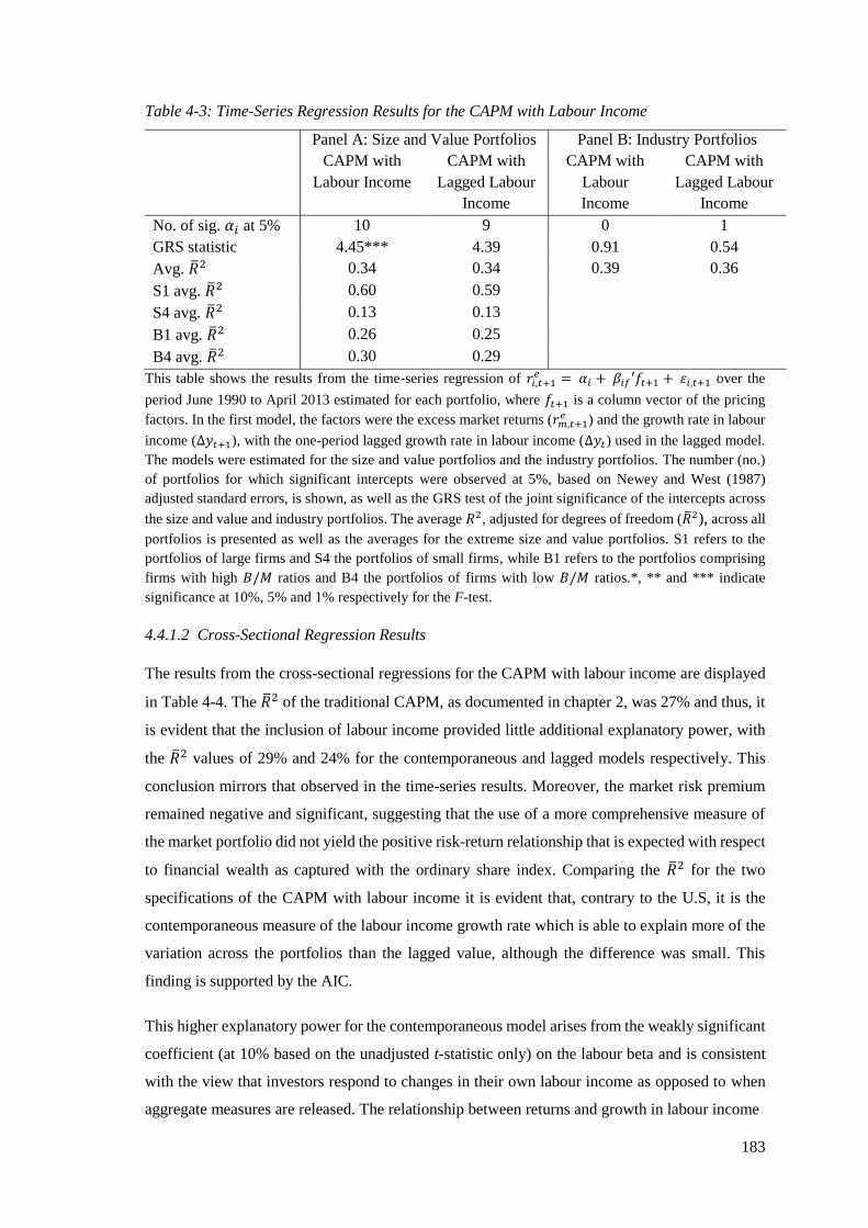
183

Table 4-3: Time-Series Regression Results for the CAPM with Labour Income


CAPM with

Labour Income

CAPM with

Lagged Labour

Income

CAPM with

Labour

Income

CAPM with

Lagged Labour

Income

No. of sig. 𝛼𝑖 at 5% 10 9 0 1

GRS statistic 4.45*** 4.39 0.91 0.54

Avg. ��2 0.34 0.34 0.39 0.36

S1 avg. ��2 0.60 0.59

S4 avg. ��2 0.13 0.13

B1 avg. ��2 0.26 0.25

B4 avg. ��2 0.30 0.29

This table shows the results from the time-series regression of 𝑟𝑖,𝑡+1𝑒 = 𝛼𝑖 + 𝛽𝑖𝑓′𝑓𝑡+1 + 휀𝑖,𝑡+1 over the

period June 1990 to April 2013 estimated for each portfolio, where 𝑓𝑡+1 is a column vector of the pricing

factors. In the first model, the factors were the excess market returns (𝑟𝑚,𝑡+1𝑒 ) and the growth rate in labour

income (Δ𝑦𝑡+1), with the one-period lagged growth rate in labour income (∆𝑦𝑡) used in the lagged model.

The models were estimated for the size and value portfolios and the industry portfolios. The number (no.)

of portfolios for which significant intercepts were observed at 5%, based on Newey and West (1987)

adjusted standard errors, is shown, as well as the GRS test of the joint significance of the intercepts across

the size and value and industry portfolios. The average 𝑅2, adjusted for degrees of freedom (��2), across all

portfolios is presented as well as the averages for the extreme size and value portfolios. S1 refers to the

portfolios of large firms and S4 the portfolios of small firms, while B1 refers to the portfolios comprising

firms with high 𝐵/𝑀 ratios and B4 the portfolios of firms with low 𝐵/𝑀 ratios.*, ** and *** indicate

significance at 10%, 5% and 1% respectively for the F-test.


The results from the cross-sectional regressions for the CAPM with labour income are displayed

in Table 4-4. The ��2 of the traditional CAPM, as documented in chapter 2, was 27% and thus, it

is evident that the inclusion of labour income provided little additional explanatory power, with

the ��2 values of 29% and 24% for the contemporaneous and lagged models respectively. This

conclusion mirrors that observed in the time-series results. Moreover, the market risk premium

remained negative and significant, suggesting that the use of a more comprehensive measure of

the market portfolio did not yield the positive risk-return relationship that is expected with respect

to financial wealth as captured with the ordinary share index. Comparing the ��2 for the two

specifications of the CAPM with labour income it is evident that, contrary to the U.S, it is the

contemporaneous measure of the labour income growth rate which is able to explain more of the

variation across the portfolios than the lagged value, although the difference was small. This

finding is supported by the AIC.

This higher explanatory power for the contemporaneous model arises from the weakly significant

coefficient (at 10% based on the unadjusted t-statistic only) on the labour beta and is consistent

with the view that investors respond to changes in their own labour income as opposed to when

aggregate measures are released. The relationship between returns and growth in labour income

184

Table 4-4: Cross-Sectional Regression Results for the CAPM with Labour Income


CAPM with

Labour Income

CAPM with

Lagged Labour

Income

CAPM with

Labour Income

CAPM with

Lagged Labour

Income

𝜆0 7.97

(5.04)***

{3.65}***

7.78

(4.78)***

{3.80}***

3.870

(4.04)***

{3.84}***

3.82

(2.92)***

(2.69)***

𝜆𝑚

-7.19

(-3.34)***

{-1.87}*

-6.57

(-3.09)***

{-1.82}*

-2.86

(-1.54)

(-0.75)

-2.98

(-1.21)

(-0.71)

𝜆𝑦 -1.25

(-1.87)*

{-1.23}

0.12

(0.60)

(0.21)

𝜆𝑦𝑡−1 0.31

(0.41)

{0.30}

0.37

(0.63)

(0.43)

𝑅2

(��2)

0.38

(0.29)

0.34

(0.24)

0.76

(0.69)

0.66

(0.55)

AIC 1.17 1.24 -1.32 -1.16


{5.02}*

9.70***

{3.41}

2.72

{0.61}

1.87

[0.69]

RMSE 1.44 1.49 0.47 0.45


{79.40}***

36.90***

{58.39}***

(3.83)

{4.23}

(2.61)

{3.09}



and nine industry portfolios, where 𝛽𝑖𝑓 is a column vector of the sensitivity of the portfolio returns to the

pricing factors (factor loadings) obtained from the time-series regressions. For the CAPM with labour

income, the factor loadings included the sensitivity to the excess market returns (𝛽𝑖𝑚) and growth rate in

labour income (𝛽𝑖∆𝑦), while in the lagged model, the sensitivity to the lagged growth rate in labour income

was used. Beneath each coefficient in round parentheses is the t-statistic computed using the Fama and

MacBeth (1973) standard errors, while the second t-statistic in curly parentheses was calculated using the

Shanken (1992) standard errors. The Wald statistic provides a test of the joint significance of the



refers to the root mean squared pricing error across the portfolios. The 𝑅2 is Jagannathan and Wang’s

(1996) cross-sectional measure of explanatory power and ��2 is adjusted for the number of pricing factors.

The AIC refers to the Akaike information criteria and was computed similarly to Jagannathan and Wang’s

(1996) 𝑅2. *, ** and *** indicate significance at 10%, 5% and 1% respectively for the various tests.

should be positive as those shares which have a higher correlation with growth in labour income

require a higher risk premium to compensate investors for the fact that these securities pay out

when labour income is already high. However, in contrast to theory the sign was found to be

negative. To understand this negative risk premium, the labour betas for each portfolio were

plotted in Figure 4-2. Consistent with the findings of Jagannathan and Wang (1996) and

Jagannathan et al. (1998) for the U.S and Japan respectively, very few of the labour betas were

185

significant (only those on S1B1 and S1B2 were significant). Jagannathan et al. (1998) argued that

this finding of insignificant labour betas does not necessarily mean that these factor loadings are

equal to zero but rather that they are measured imprecisely as reflected by high standard errors,

with the same found to be true for the South African data.

As Figure 4-2 shows, eight of the portfolios had negative betas. These negative estimates were

principally associated with the portfolios comprising large firms and those with high B/M ratios

(with the two significant betas associated with these portfolios). The finding of negative labour

betas for the large firm portfolios mirrors Jagannathan et al.’s (1998) observations for the Japanese

market and suggests that these shares represent a hedge against labour income and therefore

effectively penalise the holder in the form of a negative risk premium. At the opposite end of the

spectrum, Jagannathan et al. (1998) found the small firms to be highly positively correlated with

labour income indicating that the higher returns associated with small shares represent

compensation for their close co-movement with labour income. While the betas of the portfolios

comprising mid-sized firms in this sample appear to largely follow the trend of being larger (and

positive) compared to those on the large portfolios thus warranting a risk premium, the same

cannot be said of the small portfolios, where the betas were negative for two of the four small

firm portfolios. Thus, while Jagannathan et al. (1998) found evidence to suggest that the inclusion

of labour income could account for the size anomaly, there is only weak evidence to suggest that

the same is true for South Africa.

As mentioned in section 4.2.3, Jagannathan et al. (1998) also found some evidence to indicate

that the portfolios comprising firms with low B/M ratios were highly negatively correlated with

the growth rate in labour income whereas those with high B/M ratios were either positively

correlated or had low negative correlations, although the patterns were less definitive than across

the size-sorted portfolios. For the JSE, contradictory evidence was observed, as the value shares

(those with high B/M ratios) were those that exhibited the negative correlation with the growth

rate in labour income, as shown in Figure 4-2. Accordingly, this puzzling finding and the mixed

evidence on the size portfolios gave rise to the negative coefficient documented. This negative

risk premium on labour income was thus not only inconsistent with theory, but also failed the test

proposed by Lewellen et al. (2010) that the cross-sectional risk premium should be equal to the

time-series mean value. When the lagged labour income growth rate was used, the risk premium

was also negative, as shown in Table 4-4, but insignificant; however, it was also significantly

different from the time-series average.

186

Figure 4-2: Labour Betas for the Size and Value Portfolios

This figure plots the labour betas (𝛽𝑖∆𝑦) for each of the 16 size- and value-sorted portfolios, where the betas

were computed from the time-series regression of 𝑟𝑖,𝑡+1𝑒 = 𝛼𝑖 + 𝛽𝑖𝑚𝑟𝑚,𝑡+1

𝑒 + 𝛽𝑖∆𝑦∆𝑦𝑡+1 + 휀𝑖,𝑡+1 over the

period June 1990 to April 2013 for each of the 16 size and value portfolios, where 𝑟𝑚,𝑡+1𝑒 are the excess

market returns and ∆𝑦𝑡+1 is the growth rate in labour income. S1 refers to the portfolios of large firms and

S4 the portfolios of small firms while B1 refers to the portfolios of firms with high 𝐵/𝑀 ratios and B4 the


The finding of a significant and negative relationship between growth in labour income and

portfolio returns on the JSE, although disparate with some of the international evidence, is similar

to the results obtained by Li et al. (2011) for Australia, who found a significant negative

coefficient on the labour beta in the pricing equation and a negative R2 for the model. Moreover,

as highlighted in section 4.2.3, although the evidence regarding the importance of the growth rate

in labour income in pricing securities in Japan is strong (Jagannathan et al., 1998; Gao & Huang,

2008), the U.S evidence is mixed (Santos & Veronesi, 2006) and there was also no role for human

capital in pricing securities in the U.K (Gao & Huang, 2008).

The pricing errors from the CAPM with labour income confirmed the conclusion that this model

could not account for the cross-sectional variation in returns across the size and value portfolios,

as reflected by the significant chi-squared statistic for these models in Table-4-4. The graphical

depiction of these pricing errors in Figure 4-3 reveals that the model had substantial difficulty in

explaining the returns to value and growth portfolios, but with smaller errors for the size-sorted

portfolios on average. This serves to confirm the conclusions drawn from the analysis of the

labour betas that labour income may be able to account for some of the low returns associated

with large firms on the JSE.

187

Figure 4-3: Pricing Errors for the CAPM with Labour Income for the Size and Value Portfolios

This figure plots the pricing errors from the cross-sectional regression ��𝑖,𝑡+1𝑒 = 𝜆0 + 𝜆𝑚𝛽𝑖𝑚 + 𝜆∆𝑦𝛽𝑖∆𝑦 +

𝜂𝑖 across the 16 size and value portfolios where 𝛽𝑖𝑚 and 𝛽𝑖∆𝑦 measure the sensitivity of the portfolio returns

to the excess market returns and the growth rate in labour income respectively. S1 refers to the portfolios

of large firms and S4 the portfolios of small firms while B1 refers to the portfolios of firms with high 𝐵/𝑀

ratios and B4 the portfolios of firms with low 𝐵/𝑀 ratios.

For the industry portfolios, the ��2 values for the contemporaneous and lagged CAPM with labour

income were 69% and 55% respectively, with the pricing errors insignificant for both models.

However, none of the pricing factors were significant. These results taken together suggest that

the relatively high explanatory power of the models resulted more from the lack of variation

across the portfolios than from a model which fitted well.


The GMM results in Table 4-5 show that the conclusions drawn from the cross-sectional

regressions of the CAPM with labour income are largely robust to the estimation technique. The

transformed market risk premia were significant but negative, and the risk premium on labour

income also had a puzzling negative sign for both the contemporaneous and lagged measures of

labour income. However, the difference to the cross-sectional results where the risk premium was

only weakly significant in the contemporaneous model, both risk premia were significant based

on the GMM estimates. The J-tests of the pricing errors confirmed that neither model was able to

explain the size and value anomalies as the pricing errors were found to be significant. For the

industry portfolios, the same patterns as have been observed previously with other models were

identified in that none of the explanatory variables were significant yet the pricing errors of the

models were insignificant.

188

Table 4-5: GMM Regression Results for the CAPM with Labour Income


CAPM with

Labour Income

CAPM with

Lagged Labour

Income

CAPM with

Labour Income

CAPM with

Lagged Labour

Income

𝑏𝑚 0.05**

(2.59)

0.05***

(2.99)

0.01

(0.69)

0.00

(0.02)

𝑏∆𝑦𝑡+1 0.55**

(2.42)

0.14

(0.88)

0.29

(1.50)

𝑏∆𝑦𝑡 0.41*

(1.88)

J-statistic 37.22*** 33.21*** 7.28 5.61

𝜆𝑚 -3.91**

(-2.59)

-4.52***

(-2.97)

-0.84

(-0.70)

-0.04

(-0.03)

𝜆∆𝑦𝑡+1 -1.58**

(-2.43)

-0.40

(0.90)

𝜆∆𝑦𝑡 -1.18*

(-1.89)

-0.85

(1.53)



normalised to one. For the CAPM with labour income 𝑓𝑡+1 included the excess market returns (𝑟𝑚,𝑡+1𝑒 ) and

the growth rate in labour income (∆𝑦𝑡+1), with the one-period lagged growth rate in labour income (∆𝑦𝑡)

used in the lagged model. The models were estimated for the size and value portfolios and the industry

portfolios. The transformed risk premia (𝜆) are presented in the bottom half of the table and were computed

from the SDF coefficients as 𝜆 = −𝑣𝑎𝑟(𝑓)𝑏, where 𝑣𝑎𝑟(𝑓) is the variance of the pricing factor. Beneath

both the 𝑏’s and 𝜆’s the t-statistics are displayed in round parentheses, with the standard errors of the

transformed 𝜆’s computed using the delta method. Hansen’s (1982) J-statistic for the test of the pricing

errors is also shown. *, ** and *** indicate significance at 10%, 5% and 1% respectively for the various

tests.

The results from the tests of the CAPM with labour income thus suggest that labour income does

not appear to represent the ‘missing piece’ of the asset pricing puzzle on the JSE (or even part of

it) by providing a more comprehensive measure of total wealth. However, that is not to say that

labour income does not still affect share returns through its influence on the utility an investor

obtains from consumption. To this end, the conditioning variables which seek to capture this

relationship are still evaluated (as per the U.S and Australian studies), with the performance of

𝑐𝑎𝑦, the first of these conditioning variables, examined in the following section.

4.4.2 The Conditional CAPM and (C)CAPM with 𝒄𝒂𝒚

4.4.2.1 Estimates of 𝑐𝑎𝑦

The results for the ADF and KPSS tests on consumption, asset wealth and labour income are

shown in panel A of Table 4-6. The results across both tests indicated that the series were non-

stationary in levels but stationary in first differences. As all the variables were integrated of the

same order, the cointegration tests were undertaken; the results of which are shown in panel B of

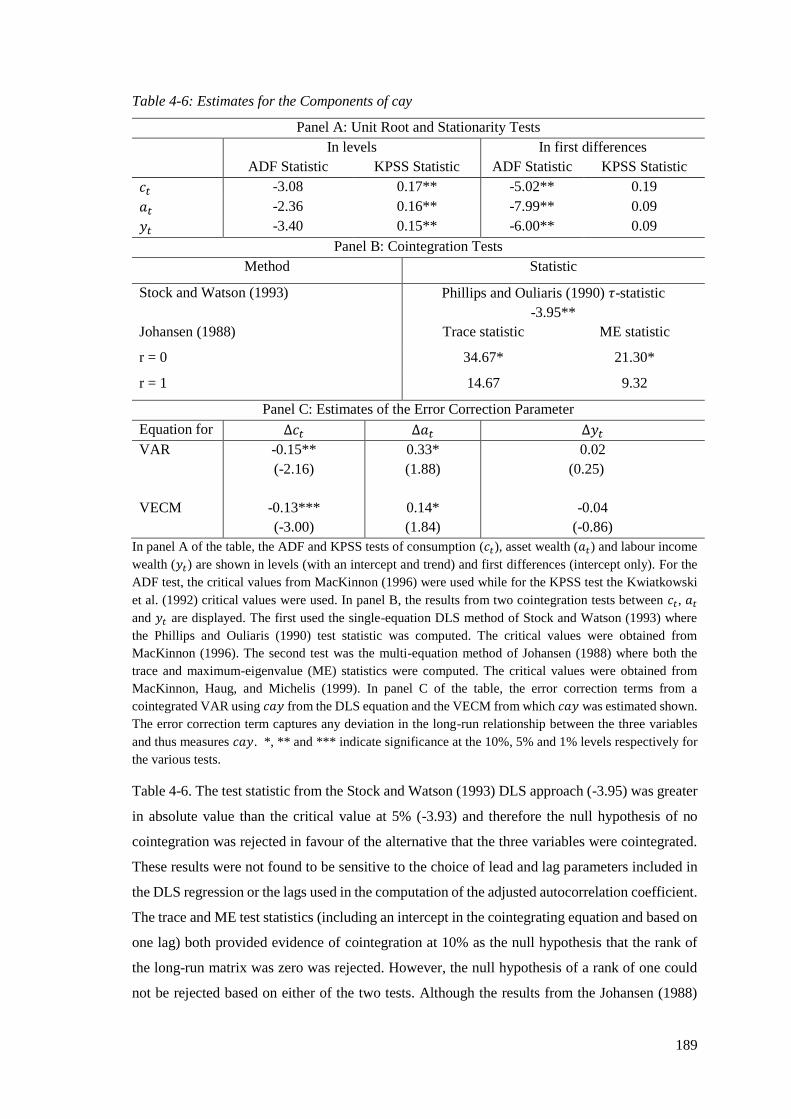
189

Table 4-6: Estimates for the Components of cay

Panel A: Unit Root and Stationarity Tests

In levels In first differences

ADF Statistic KPSS Statistic ADF Statistic KPSS Statistic

𝑐𝑡 -3.08 0.17** -5.02** 0.19

𝑎𝑡 -2.36 0.16** -7.99** 0.09

𝑦𝑡 -3.40 0.15** -6.00** 0.09

Panel B: Cointegration Tests

Method Statistic

Stock and Watson (1993) Phillips and Ouliaris (1990) 𝜏-statistic

-3.95**

Johansen (1988) Trace statistic ME statistic

r = 0 34.67* 21.30*

r = 1 14.67 9.32

Panel C: Estimates of the Error Correction Parameter

Equation for Δ𝑐𝑡 Δ𝑎𝑡 Δ𝑦𝑡

VAR -0.15**

(-2.16)

0.33*

(1.88)

0.02

(0.25)

VECM -0.13***

(-3.00)

0.14*

(1.84)

-0.04

(-0.86)

In panel A of the table, the ADF and KPSS tests of consumption (𝑐𝑡), asset wealth (𝑎𝑡) and labour income

wealth (𝑦𝑡) are shown in levels (with an intercept and trend) and first differences (intercept only). For the

ADF test, the critical values from MacKinnon (1996) were used while for the KPSS test the Kwiatkowski

et al. (1992) critical values were used. In panel B, the results from two cointegration tests between 𝑐𝑡, 𝑎𝑡

and 𝑦𝑡 are displayed. The first used the single-equation DLS method of Stock and Watson (1993) where

the Phillips and Ouliaris (1990) test statistic was computed. The critical values were obtained from

MacKinnon (1996). The second test was the multi-equation method of Johansen (1988) where both the

trace and maximum-eigenvalue (ME) statistics were computed. The critical values were obtained from

MacKinnon, Haug, and Michelis (1999). In panel C of the table, the error correction terms from a

cointegrated VAR using 𝑐𝑎𝑦 from the DLS equation and the VECM from which 𝑐𝑎𝑦 was estimated shown.

The error correction term captures any deviation in the long-run relationship between the three variables

and thus measures 𝑐𝑎𝑦. *, ** and *** indicate significance at the 10%, 5% and 1% levels respectively for

the various tests.

Table 4-6. The test statistic from the Stock and Watson (1993) DLS approach (-3.95) was greater

in absolute value than the critical value at 5% (-3.93) and therefore the null hypothesis of no

cointegration was rejected in favour of the alternative that the three variables were cointegrated.

These results were not found to be sensitive to the choice of lead and lag parameters included in

the DLS regression or the lags used in the computation of the adjusted autocorrelation coefficient.

The trace and ME test statistics (including an intercept in the cointegrating equation and based on

one lag) both provided evidence of cointegration at 10% as the null hypothesis that the rank of

the long-run matrix was zero was rejected. However, the null hypothesis of a rank of one could

not be rejected based on either of the two tests. Although the results from the Johansen (1988)

190

cointegration tests only provide weak evidence of the existence of a long-run relationship between

consumption, asset wealth and labour income, they do confirm the results obtained from the

Phillips and Ouliaris (1990) test on the residuals from the DLS equation. The finding of

cointegration is consistent with the results obtained in the U.S, Australia, the U.K, Canada and

Japan (Lettau & Ludvigson, 2001a; Ioannidis et al., 2006; Gao & Huang, 2008; Li et al., 2011).

The estimates from the long-run relationship based on the DLS method are as follows

𝑐𝑡 = 2.22 + 0.24𝑎𝑡 + 0.51𝑦𝑡, (4.25)

(8.77) (6.10) (9.50)

with the t-statistics based on the Newey and West (1987) standard errors shown in parentheses.

The estimates from the VECM are

𝑐𝑡 = 1.69 + 0.32𝑎𝑡 + 0.48𝑦𝑡. (4.26)

The point estimates of the coefficients are not substantially different across the two methods,

which is consistent with the theoretical similarities between the two approaches, given that only

one cointegrating equation was found under the single-equation test. The coefficients in the

cointegrating vector summed to 0.75 and 0.8 for equations 4.25 and 4.26 respectively. Although

this is less than the theoretical value of one, Lettau and Ludvigson (2010) suggested that such a

finding is to be expected given that proxies for the true variables are used. Asset wealth and labour

income had positive relationships with consumption, with the t-statistics from the DLS equation

confirming that the relationships were significant. The relative magnitudes of the coefficients in

the equations indicate that labour income had a stronger relationship with consumption than asset

wealth. The findings that labour income is a more important driver of consumption than asset

wealth in South Africa mirrors the findings of Lettau and Ludvigson (2001a), Hahn and Lee

(2006) and Rasmussen (2006) for the U.S and Gao and Huang (2008) for the U.K and Japan. In

contrast, for Canada and Australia Ioannidis et al. (2006) and Li et al. (2011) for Australia

identified the relationship between asset wealth and consumption to be stronger than that for

labour income and consumption.

Any deviations in the long-run relationship between the three variables, which is captured by 𝑐𝑎𝑦,

must forecast movements in one of the three variables and thus it was considered of value to

determine whether these deviations represent transitory movements in consumption, asset wealth

and/or income. For this purpose, a cointegrated VAR was estimated using 𝑐𝑎𝑦 from the DLS

equation, while the VECM from Johansen’s (1988) cointegration test was also examined. As

shown in panel C of Table 4-6, the error correction mechanism was significant at 5% and 10% in

the consumption and asset wealth equations respectively under both models. This indicates that

191

short-term deviations in the long-run relationship can be viewed as transitory movements in these

two variables but not in labour income. The positive coefficient in the asset wealth equation is

consistent with the theory that an increase in 𝑐𝑎𝑦 should lead to an increase in asset wealth and

mirrors the findings of Lettau and Ludvigson (2001a) and Hahn and Lee (2006). Assuming asset

wealth and share returns are positively correlated, this result suggests that 𝑐𝑎𝑦 may have power

to explain future returns. The finding of a significant coefficient on consumption does differ from

the results of both Lettau and Ludvigson (2001a) and Hahn and Lee (2006) suggesting that in the

South African market consumption adjusts to restore equilibrium more than asset wealth.

The results for the remaining analyses using 𝑐𝑎𝑦 were found to be robust to the computational

approach used; a finding which is not only consistent with Rasmussen’s (2006) results but also is

logical given the similarity in the long-run relationships in 4.25 and 4.26. Only the results based

on the estimate of 𝑐𝑎𝑦 from the DLS method are shown hereafter in the interest of brevity.

4.4.2.2 Descriptive Statistics and the Predictive Power of 𝑐𝑎𝑦

The descriptive statistics of 𝑐𝑎𝑦 are shown in Table 4-7. The mean of the series is higher than

that observed in the U.S and Australia (Lettau & Ludvigson, 2001a; Li et al., 2011), suggesting

that, on average, the deviation of the variables from the long-run relationship was substantial. 𝑐𝑎𝑦

exhibits similar properties to the 𝐷/𝑃 and 𝐸/𝑃 ratios examined in chapter 3 as it does not vary

substantially over time and is persistent as captured by the autocorrelation coefficient of 0.78.

However, the fact that 𝑐𝑎𝑦 is a residual from a cointegrating relationship means that it is stationary

despite the relatively high persistence. These properties of low variation and high first-order

autocorrelation match those documented for 𝑐𝑎𝑦 in the in the U.S, Australia, U.K and Japan

(Lettau & Ludvigson, 2001a; Li et al., 2011; Gao & Huang, 2008).

𝑐𝑎𝑦 had very low correlations with the excess real market return, term spread and relative T-bill

yield, as shown in panel B of Table 4-7. This suggests that if 𝑐𝑎𝑦 can predict share returns, it

contains different information from the spread and relative T-Bill yield, which had some success

in predicting returns. In contrast, 𝑐𝑎𝑦 had a high negative correlation with both the 𝐷/𝑃 and 𝐸/𝑃

ratios, with these two financial ratios themselves highly correlated, as noted in chapter 3. These

strong relationships with 𝐷/𝑃 and 𝐸/𝑃 suggest that if 𝑐𝑎𝑦 can predict future business cycles, it

may track analogous predictable components of the share returns captured by the financial ratios.

However, the relatively high persistence in these series may also account for the high co-

movement observed.

The forecasting results for 𝑐𝑎𝑦 for the various forecasting periods are documented in Table 4-8.

When 𝑐𝑎𝑦 was the sole explanatory variable a significant coefficient was obtained for the one-

192

Table 4-7: Summary Statistics of cay

𝑐𝑎𝑦


Avg. 2.22

Std. Dev. 0.03

𝜌(1) 0.78

Panel B: Correlation Coefficients

𝑟𝑚𝑒 0.16

𝑟𝑒𝑙𝑎𝑡𝑖𝑣𝑒 -0.30

𝑠𝑝𝑟𝑒𝑎𝑑 0.10

𝐷/𝑃 0.54

𝐸/𝑃 0.57

In panel A of this table the descriptive statistics of the consumption aggregate wealth ratio, 𝑐𝑎𝑦, over the

period July 1990 to April 2013 are shown. These include the average (avg.), standard deviation (std. dev.)

and first-order autocorrelation (𝜌(1)). In panel B, the correlation coefficients between 𝑐𝑎𝑦 and the

traditional forecasting variables – the term spread (𝑠𝑝𝑟𝑒𝑎𝑑), relative T-bill (𝑟𝑒𝑙𝑎𝑡𝑖𝑣𝑒), 𝐷/𝑃, 𝐸/𝑃 and the

lagged excess market returns (𝑟𝑚𝑒 ) are presented.

Table 4-8: Forecasts of Multiple Quarter Excess Real Market Returns using cay

Forecast horizon (H) in quarters

1 2 4 6 8 12

𝑐𝑎𝑦 2.88

(3.38)***

[0.08]

{0.08}

3.98

(2.98)***

[0.07]

{0.09}

6.90

(3.36)***

[0.11]

{0.07}

8.13

(2.21)**

[0.10]

{0.04}

9.89

(2.64)***

[0.12]

{0.03}

15.27

(4.08)***

[0.22]

{0.05}



𝐷/𝑃

𝑐𝑎𝑦

0.19

(0.15)

2.58

(2.05)**

0.73

(0.59)

2.80

(2.36)**

[0.11]

{0.06}

0.54

(0.12)

3.59

(1.69)*

2.41

(0.85)

3.19

(1.78)*

[0.10]

{0.07}

1.28

(0.44)

5.96

(1.79)*

4.86

(1.38)

5.30

(2.09)**

[0.17]

{0.09}

-0.17

(-0.06)

7.97

(2.21)**

8.63

(2.04)**

4.26

(1.15)

[0.23]

{0.08}

-5.24

(-1.57)

5.09

(1.67)*

10.35

(2.19)**

2.89

(0.74)

[0.29]

{0.06}

-5.68

(-1.39)

-0.53

(-0.18)

17.88

(3.29)***

3.10

(0.61)

[0.46]

{0.07}



and 𝑧𝑡 is the column vector of predictor variables. For the first regression 𝑧𝑡 included the consumption

aggregate wealth ratio, 𝑐𝑎𝑦, while for the second regression this was combined with the term spread

(𝑠𝑝𝑟𝑒𝑎𝑑), relative T-bill (𝑟𝑒𝑙𝑎𝑡𝑖𝑣𝑒) and 𝐷/𝑃. Beneath each coefficient in round parentheses is the t-

statistic computed using the Newey and West (1987) standard errors. The regression 𝑅2, adjusted for

degrees of freedom, ��2, is shown in square parentheses, with Hodrick’s (1992) ��2 presented thereunder in

curly parentheses. *, ** and *** indicate significance at the 10%, 5% and 1% levels respectively for the t-

tests.

quarter ahead horizon, consistent with the conclusions drawn from the error correction

mechanism that 𝑐𝑎𝑦 can forecast future returns. The coefficient was positive in accordance with

193

the theoretical relationship that if market returns are forecast to increase in the future, then

investors who desire smooth consumption levels will allow consumption to temporarily increase

above its long-term relationship with asset wealth and labour income on the basis that future

consumption will be supported from higher future returns. The opposite is true if returns are

expected to decrease, with investors reducing consumption below the long-term level with asset

wealth and labour income so as to protect future consumption levels against lower returns (Lettau

& Ludvigson, 2001a). The explanatory power for the one-quarter ahead returns was 8%, as

measured by ��2, which is comparable to the 9% and 8% documented by Lettau and Ludvigson

(2001a, 2010) in their studies of the U.S. Gao and Huang (2008) obtained a lower ��2 for the U.K

of 4%, and a 0% ��2 for Japan where 𝑐𝑎𝑦 had no explanatory power. In chapter 3 the term spread

was the most successful variable for predicting one-period ahead returns and was found to be able

to explain 4% of the variation in one-quarter ahead returns. Thus, it is clearly evident that 𝑐𝑎𝑦 by

itself is a superior predictor of one-quarter ahead returns on the JSE than any of the traditional

variables.

The graph in Figure 4-4 confirms the ability of 𝑐𝑎𝑦 to predict the one-quarter ahead excess real

market returns. For example, during the Asian crisis of 1998/1999, the bursting of the dot-com

bubble in 2001 and the 2008/2009 financial crisis, 𝑐𝑎𝑦 and the market moved together closely.

However, 𝑐𝑎𝑦 appeared to move less closely with the market during the period 2006 to 2007.

These trends indicate that 𝑐𝑎𝑦 had more success in predicting market movements during financial

crises and volatile markets than during bull runs, which mirrors some of the evidence presented

by Lettau and Ludvigson (2001a) for the U.S.

As the results in Table 4-8 confirm, the success of 𝑐𝑎𝑦 in forecasting share returns was not only

limited to the short-run, as it was able to explain 12% and 22% of the variation at eight- and 12-

quarters ahead, although this is not as substantial as the predictive power documented by Lettau

and Ludvigson (2010) for the U.S of 28% and 34% for the same horizons. However, after

accounting for the persistent nature of the measure, the explanatory power was notably reduced

over longer horizons, as captured by Hodrick’s (1992) ��2. This finding does differ from that

documented by both Rasmussen (2006) and Lettau and Ludvigson (2010) who found that 𝑐𝑎𝑦

retained its forecasting power over long-horizons on the U.S market, even after accounting for

the persistence in the series.

The joint predictive power of 𝑐𝑎𝑦 with the traditional forecasting variables in this sample was

also assessed, as shown in Table 4-8 (the reasonably high co-movement between 𝑐𝑎𝑦 and 𝐷/𝑃

was not found to induce multicollinearity in these regressions). As can be seen 𝑐𝑎𝑦 retained its

significance but only for one-, two and four quarters ahead. Lettau and Ludvigson (2010) found

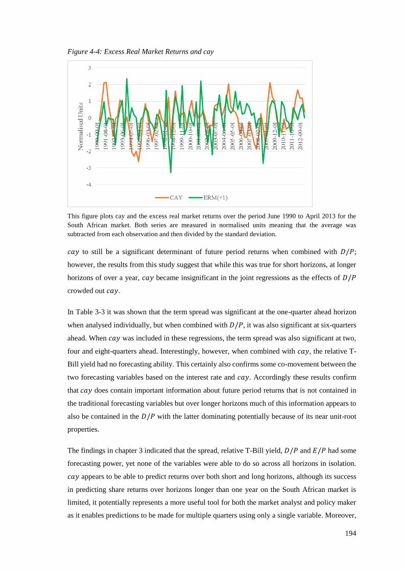
194

Figure 4-4: Excess Real Market Returns and cay

This figure plots cay and the excess real market returns over the period June 1990 to April 2013 for the

South African market. Both series are measured in normalised units meaning that the average was

subtracted from each observation and then divided by the standard deviation.

𝑐𝑎𝑦 to still be a significant determinant of future period returns when combined with 𝐷/𝑃;

however, the results from this study suggest that while this was true for short horizons, at longer

horizons of over a year, 𝑐𝑎𝑦 became insignificant in the joint regressions as the effects of 𝐷/𝑃

crowded out 𝑐𝑎𝑦.

In Table 3-3 it was shown that the term spread was significant at the one-quarter ahead horizon

when analysed individually, but when combined with 𝐷/𝑃, it was also significant at six-quarters

ahead. When 𝑐𝑎𝑦 was included in these regressions, the term spread was also significant at two,

four and eight-quarters ahead. Interestingly, however, when combined with 𝑐𝑎𝑦, the relative T-

Bill yield had no forecasting ability. This certainly also confirms some co-movement between the

two forecasting variables based on the interest rate and 𝑐𝑎𝑦. Accordingly these results confirm

that 𝑐𝑎𝑦 does contain important information about future period returns that is not contained in

the traditional forecasting variables but over longer horizons much of this information appears to

also be contained in the 𝐷/𝑃 with the latter dominating potentially because of its near unit-root

properties.

The findings in chapter 3 indicated that the spread, relative T-Bill yield, 𝐷/𝑃 and 𝐸/𝑃 had some

forecasting power, yet none of the variables were able to do so across all horizons in isolation.

𝑐𝑎𝑦 appears to be able to predict returns over both short and long horizons, although its success

in predicting share returns over horizons longer than one year on the South African market is

limited, it potentially represents a more useful tool for both the market analyst and policy maker

as it enables predictions to be made for multiple quarters using only a single variable. Moreover,

195

in the context of asset pricing a variable which can predict business cycles at varying frequencies

may also be able to more successfully capture changes in risk over the cycles than the conditioning

variables utilised in chapter 3. The extent to which this is true is examined in more detail in the

next section.


Prior to estimating the models, the correlation between the pricing factors in the two models was

examined. As shown in Table C-3 in the appendix (p. 329), there was little co-movement between

the factors and as such multicollinearity was not considered a concern. For the size- and value-

sorted portfolios, the ��2 for the conditional CAPM was 17% and for the (C)CAPM it was 34%,

as shown in Table 4-9. Therefore, the time-varying consumption CAPM, using 𝑐𝑎𝑦 to predict

business cycles, was better able to capture the variation in returns across the portfolios than the

time-varying CAPM. The ranking of the models based on the AIC confirms this conclusion. This

finding is consistent with the empirical results of Lettau and Ludvigson (2001b) for the U.S and

Li et al. (2011) for Australia, but does contrast with Gao and Huang (2008) who found that the

market portfolio was a more important determinant of returns in the U.K and Japanese markets

than was consumption growth. The explanatory power of the (C)CAPM in South Africa was still

lower than that obtained in the U.S, where the model was able to explain approximately 66% of

the variation across the size- and value-sorted portfolios in the tests of Lettau and Ludvigson

(2001b) and between 43% and 59% from the results of Rasmussen (2006), depending on the

period examined. However, the explanatory power is in a similar range to that documented for

Australia of 28% (Li et al., 2011), the U.K of 39% and Japan of 13% (Gao & Huang, 2008).

The explanatory power of the (C)CAPM exceeds that obtained for the consumption CAPM of -

0.05% and traditional CAPM of 27%, but was still lower than the Fama and French (1993) model,

which was able to explain 70% of the variation across the size- and value-sorted portfolios.

However, as noted in section 4.2.4.1, this trend has been documented for most of the countries

where the (C)CAPM with 𝑐𝑎𝑦 has been tested, including the U.S, Australia, the U.K and Japan.

The conditional CAPM, using traditional forecasting variables, tested in chapter 3, had higher

explanatory power on the South African market than the models utilising 𝑐𝑎𝑦 as the conditioning

variables. At face value this appears to indicate that 𝑐𝑎𝑦 is less successful at capturing the time-

variation in risk (and return) across the business cycles; however, as noted in chapter 3, these ��2

measures are not a true reflection of the model’s explanatory power because they reflect a

significant role for the market portfolio in explaining differences in returns across the portfolios;

yet, a negative relationship was observed between risk and return which is entirely inconsistent

with theory. To assess whether the same may be true for the ��2 values from these models, the

signs and significance of the pricing factors in these asset pricing models were evaluated.

196

Table 4-9: Cross-Sectional Regression Results for the Conditional Models with cay


Conditional

CAPM

(C)CAPM (C)CAPM with

Size and Value

Conditional

CAPM

(C)CAPM

𝜆0 7.06

(4.71)***

{4.05}***

4.03

(3.57)***

{2.42}**

3.58

(3.12)***

{2.53}**

2.80

(1.80)*

{1.75}*

0.86

(1.05)

{1.02}

𝜆𝑚 -5.27

(-2.73)***

{-2.33}**

-1.97

(-0.84)

{-0.49}

𝜆𝑐𝑎𝑦 -0.87

(-1.24)

{-1.06}

-1.34

(-1.57)

{-0.96}

-1.06

(-1.15)

{-0.93}

0.10

(0.15)

{0.10}

0.53

(0.84)

{0.54}

𝜆∆𝑐 0.95

(2.20)**

{1.69}*

0.48

(0.97)

{0.78}

-0.03

(-0.12)

{-0.05}

𝜆𝑚𝑐𝑎𝑦 1.22

(0.27)

{0.23}

-2.22

(-0.53)

{-0.29}

𝜆∆𝑐𝑐𝑎𝑦 1.80

(2.34)**

{1.94}*

1.98

(1.68)*

{1.33}

0.24

(0.15)

{0.12}

2.61

(3.65)***

{2.91}***

2.40

(2.76)***

{2.20}**

197

𝑅2

(��2)

0.33

(0.17)

0.47

(0.34)

0.86

(0.78)

0.72

(0.56)

0.65

(0.44)

AIC 1.37 1.14 0.09 -1.14 -0.90

Wald statistic 9.07**

{6.63}*

10.27**

{4.70}

23.40**

{20.90}**

1.00

{0.33}

0.75

{0.31}

RMSE 1.50 1.28 0.70 0.45 0.59


{52.92}***

34.38***

{74.84}***

(8.54)

{6.66}

4.29

{4.53}

4.20

{4.44}

This table reports the coefficients from the Fama and MacBeth (1973) cross-sectional regression ��𝑖,𝑡+1𝑒 = 𝜆0 + 𝜆𝑓′𝛽𝑖𝑓 + 𝜂𝑖, estimated over the period June 1990 to April 2013

across the 16 size and value portfolios and nine industry portfolios, where 𝛽𝑖𝑓 is a column vector of the sensitivity of the portfolio returns to the pricing factors obtained from

the time-series regressions. For the conditional CAPM, the factor loadings were the sensitivity of the portfolio returns to the excess real market returns (𝛽𝑝𝑚), the sensitivity to

the consumption aggregate wealth ratio (𝛽𝑖𝑐𝑎𝑦) and the scaled excess real market returns (𝛽𝑖𝑝𝑚𝑐𝑎𝑦). For the (C)CAPM, the factor loadings were the sensitivity of the portfolio

returns to the growth rate in consumption (𝛽𝑖∆𝑐), 𝛽𝑖𝑐𝑎𝑦 and the sensitivity to the scaled consumption growth rate (𝛽𝑖∆𝑐𝑐𝑎𝑦). Finally, for the (C)CAPM with size and value, the

sensitivity to the two Fama and French (1993) factors - the returns on a zero-cost portfolio long small firm shares and short big firm shares (𝛽𝑖𝑆𝑀𝐵) and a zero-cost portfolio

long firms with high 𝐵/𝑀 ratios and short firms with low 𝐵/𝑀 ratios (𝛽𝑖𝐻𝑀𝐿) – were also included. Beneath each coefficient in round parentheses is the t-statistic computed

using the Fama and MacBeth (1973) standard errors, while the second t-statistic in curly parentheses was calculated using the Shanken (1992) standard errors. The Wald statistic

provides a test of the joint significance of the coefficients and the Q-statistic tests the joint significance of the model pricing errors. The values of both of these statistics computed

using Shanken’s (1992) standard errors are shown in curly parentheses. RMSE refers to the root mean squared pricing error across the portfolios. The 𝑅2 is Jagannathan and

Wang’s (1996) cross-sectional measure of explanatory power and ��2 is adjusted for the number of pricing factors. The AIC refers to the Akaike information criteria and was

computed similarly to Jagannathan and Wang’s (1996) 𝑅2. *, ** and *** indicate significance at 10%, 5% and 1% respectively for the various tests.

198

For the conditional CAPM and (C)CAPM the intercepts were significant; a result which was also

observed by Lettau and Ludvigson (2001b) and Li et al. (2011) and which, as explained

previously, contests the validity of both of these models. Consumption growth was priced

reflecting that shares with higher exposure to the consumption growth rate earned higher returns.

The significant role for consumption growth in explaining the cross-sectional returns does

contrast with the international evidence but is similar to that observed for the static consumption

CAPM in chapter 3, although the evidence in that model was weaker. Similarly, to the findings

of Lettau and Ludvigson (2001b), Rasmussen (2006) and Gao and Huang (2008), the time-

varying beta coefficient was significant suggesting that consumption risk did vary across business

cycles, while there was little evidence of time-varying returns arising from consumption

smoothing.

The conditional consumption betas, computed as the sum of the consumption and scaled

consumption betas from the (C)CAPM, are displayed in Figure 4-5 (in this case both betas were

examined together as they were both found to be priced in the cross-section). As can be seen,

several of the portfolios comprising value shares (denoted B1) exhibited higher conditional

consumption betas than the portfolios of growth shares (denoted B4), which is consistent with the

positive coefficients in the cross-sectional regression. However, there was less evidence to

suggest that the portfolios comprising smaller firms (denoted S4) exhibited greater conditional

consumption betas than larger shares (denoted S1) as would be the case if this model was able to

account for both anomalies.

To explore this dynamic further, the conditional consumption betas were estimated for each

portfolio in a good state and a bad state. Based on the findings from the predictive regressions

𝑐𝑎𝑦 was high when risk aversion/ risk is high, and thus a bad state is one where 𝑐𝑎𝑦 was higher

than average while a ‘good state’ is one where 𝑐𝑎𝑦 was lower than average. Accordingly, the

former were identified when 𝑐𝑎𝑦 was half a standard deviation above the average, and the latter

when 𝑐𝑎𝑦 was half a standard deviation below the average. The betas in each state for the value

and growth portfolios at each size quartile are shown in Figure 4-6 while those for the small and

large firm portfolios at each 𝐵/𝑀 quartile are depicted in Figure 4-7. In the first two graphs of

Figure 4-6, it is evident that the value portfolios exhibited higher betas in bad states compared to

good states, while the opposite was true for the growth shares in the same size quintile. Such

evidence is consistent with the view that value shares earned higher returns to compensate

investors for the greater risk of holding these shares when risk is high (as captured by a high value

of 𝑐𝑎𝑦). That is, these shares need to pay investors a high premium because they are the opposite

of insurance as they perform poorly when investors are largely risk averse (in bad states). The

converse is true for growth shares. However, this relationship does not hold perfectly in the South

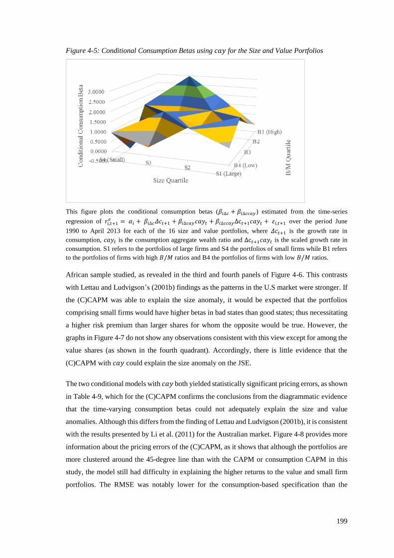
199

Figure 4-5: Conditional Consumption Betas using 𝑐𝑎𝑦 for the Size and Value Portfolios

This figure plots the conditional consumption betas (𝛽𝑖∆𝑐 + 𝛽𝑖∆𝑐𝑐𝑎𝑦) estimated from the time-series

regression of 𝑟𝑖,𝑡+1𝑒 = 𝛼𝑖 + 𝛽𝑖∆𝑐𝛥𝑐𝑡+1 + 𝛽𝑖∆𝑐𝑎𝑦𝑐𝑎𝑦𝑡 + 𝛽𝑖∆𝑐𝑐𝑎𝑦Δc𝑡+1𝑐𝑎𝑦𝑡 + 휀𝑖,𝑡+1 over the period June

1990 to April 2013 for each of the 16 size and value portfolios, where 𝛥𝑐𝑡+1 is the growth rate in

consumption, 𝑐𝑎𝑦𝑡 is the consumption aggregate wealth ratio and Δc𝑡+1𝑐𝑎𝑦𝑡 is the scaled growth rate in

consumption. S1 refers to the portfolios of large firms and S4 the portfolios of small firms while B1 refers


African sample studied, as revealed in the third and fourth panels of Figure 4-6. This contrasts

with Lettau and Ludvigson’s (2001b) findings as the patterns in the U.S market were stronger. If

the (C)CAPM was able to explain the size anomaly, it would be expected that the portfolios

comprising small firms would have higher betas in bad states than good states; thus necessitating

a higher risk premium than larger shares for whom the opposite would be true. However, the

graphs in Figure 4-7 do not show any observations consistent with this view except for among the

value shares (as shown in the fourth quadrant). Accordingly, there is little evidence that the

(C)CAPM with 𝑐𝑎𝑦 could explain the size anomaly on the JSE.

The two conditional models with 𝑐𝑎𝑦 both yielded statistically significant pricing errors, as shown

in Table 4-9, which for the (C)CAPM confirms the conclusions from the diagrammatic evidence

that the time-varying consumption betas could not adequately explain the size and value

anomalies. Although this differs from the finding of Lettau and Ludvigson (2001b), it is consistent

with the results presented by Li et al. (2011) for the Australian market. Figure 4-8 provides more

information about the pricing errors of the (C)CAPM, as it shows that although the portfolios are

more clustered around the 45-degree line than with the CAPM or consumption CAPM in this

study, the model still had difficulty in explaining the higher returns to the value and small firm

portfolios. The RMSE was notably lower for the consumption-based specification than the

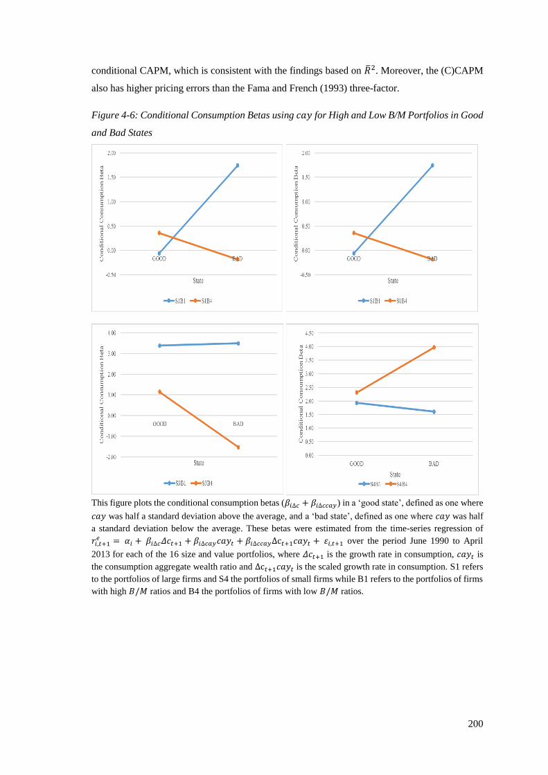
200

conditional CAPM, which is consistent with the findings based on ��2. Moreover, the (C)CAPM

also has higher pricing errors than the Fama and French (1993) three-factor.

Figure 4-6: Conditional Consumption Betas using 𝑐𝑎𝑦 for High and Low B/M Portfolios in Good

and Bad States

This figure plots the conditional consumption betas (𝛽𝑖∆𝑐 + 𝛽𝑖∆𝑐𝑐𝑎𝑦) in a ‘good state’, defined as one where

𝑐𝑎𝑦 was half a standard deviation above the average, and a ‘bad state’, defined as one where 𝑐𝑎𝑦 was half

a standard deviation below the average. These betas were estimated from the time-series regression of

𝑟𝑖,𝑡+1𝑒 = 𝛼𝑖 + 𝛽𝑖∆𝑐𝛥𝑐𝑡+1 + 𝛽𝑖∆𝑐𝑎𝑦𝑐𝑎𝑦𝑡 + 𝛽𝑖∆𝑐𝑐𝑎𝑦Δc𝑡+1𝑐𝑎𝑦𝑡 + 휀𝑖,𝑡+1 over the period June 1990 to April

2013 for each of the 16 size and value portfolios, where 𝛥𝑐𝑡+1 is the growth rate in consumption, 𝑐𝑎𝑦𝑡 is

the consumption aggregate wealth ratio and Δc𝑡+1𝑐𝑎𝑦𝑡 is the scaled growth rate in consumption. S1 refers

to the portfolios of large firms and S4 the portfolios of small firms while B1 refers to the portfolios of firms

with high 𝐵/𝑀 ratios and B4 the portfolios of firms with low 𝐵/𝑀 ratios.

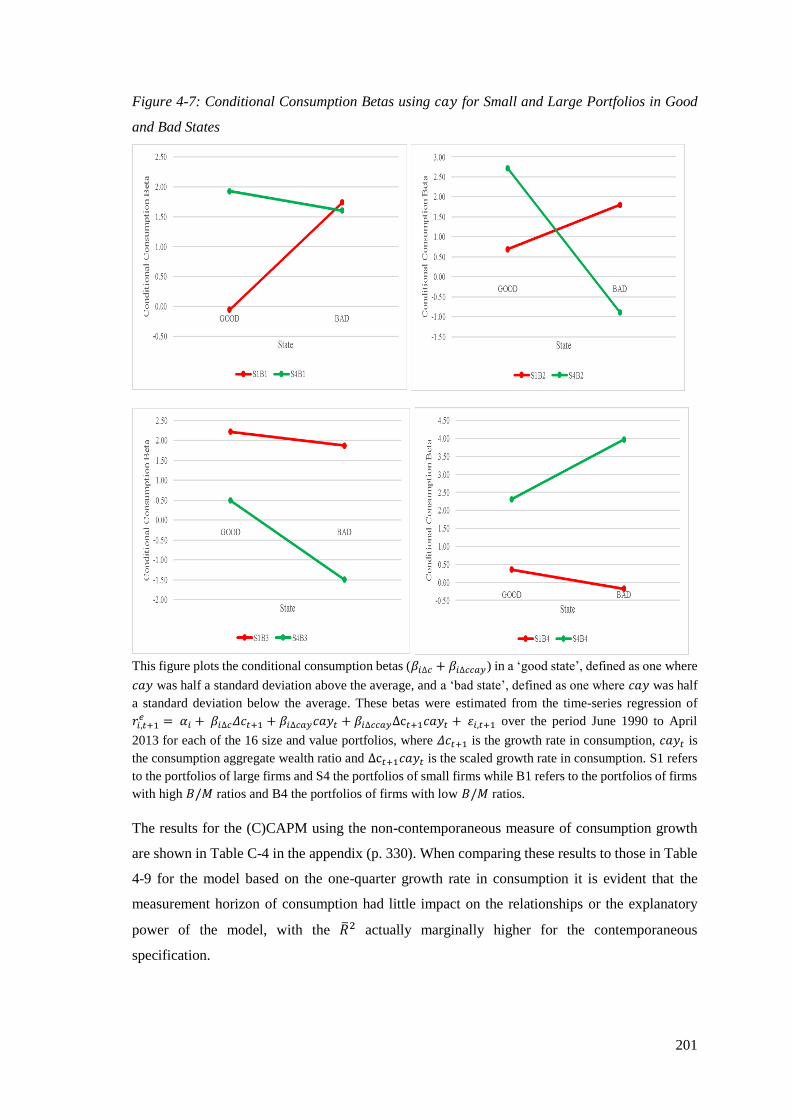
201

Figure 4-7: Conditional Consumption Betas using 𝑐𝑎𝑦 for Small and Large Portfolios in Good

and Bad States

This figure plots the conditional consumption betas (𝛽𝑖∆𝑐 + 𝛽𝑖∆𝑐𝑐𝑎𝑦) in a ‘good state’, defined as one where

𝑐𝑎𝑦 was half a standard deviation above the average, and a ‘bad state’, defined as one where 𝑐𝑎𝑦 was half

a standard deviation below the average. These betas were estimated from the time-series regression of

𝑟𝑖,𝑡+1𝑒 = 𝛼𝑖 + 𝛽𝑖∆𝑐𝛥𝑐𝑡+1 + 𝛽𝑖∆𝑐𝑎𝑦𝑐𝑎𝑦𝑡 + 𝛽𝑖∆𝑐𝑐𝑎𝑦Δc𝑡+1𝑐𝑎𝑦𝑡 + 휀𝑖,𝑡+1 over the period June 1990 to April

2013 for each of the 16 size and value portfolios, where 𝛥𝑐𝑡+1 is the growth rate in consumption, 𝑐𝑎𝑦𝑡 is

the consumption aggregate wealth ratio and Δc𝑡+1𝑐𝑎𝑦𝑡 is the scaled growth rate in consumption. S1 refers



The results for the (C)CAPM using the non-contemporaneous measure of consumption growth

are shown in Table C-4 in the appendix (p. 330). When comparing these results to those in Table

4-9 for the model based on the one-quarter growth rate in consumption it is evident that the

measurement horizon of consumption had little impact on the relationships or the explanatory

power of the model, with the ��2 actually marginally higher for the contemporaneous

specification.

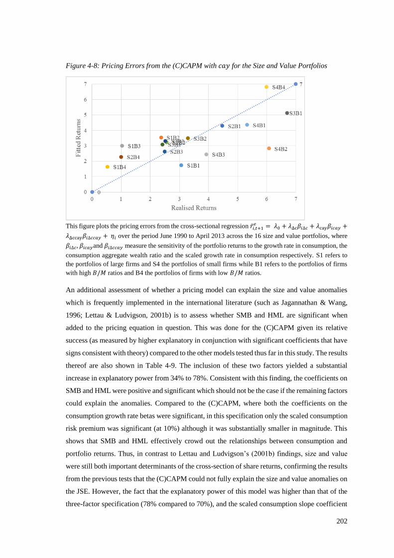
202

Figure 4-8: Pricing Errors from the (C)CAPM with 𝑐𝑎𝑦 for the Size and Value Portfolios


𝑒 = 𝜆0 + 𝜆Δc𝛽𝑖∆𝑐 + 𝜆cay𝛽𝑖𝑐𝑎𝑦 +

𝜆Δccay𝛽𝑖∆𝑐𝑐𝑎𝑦 + 𝜂𝑖 over the period June 1990 to April 2013 across the 16 size and value portfolios, where

𝛽𝑖∆𝑐, 𝛽𝑖𝑐𝑎𝑦and 𝛽𝑖∆𝑐𝑐𝑎𝑦 measure the sensitivity of the portfolio returns to the growth rate in consumption, the

consumption aggregate wealth ratio and the scaled growth rate in consumption respectively. S1 refers to

the portfolios of large firms and S4 the portfolios of small firms while B1 refers to the portfolios of firms


An additional assessment of whether a pricing model can explain the size and value anomalies

which is frequently implemented in the international literature (such as Jagannathan & Wang,

1996; Lettau & Ludvigson, 2001b) is to assess whether SMB and HML are significant when

added to the pricing equation in question. This was done for the (C)CAPM given its relative

success (as measured by higher explanatory in conjunction with significant coefficients that have

signs consistent with theory) compared to the other models tested thus far in this study. The results

thereof are also shown in Table 4-9. The inclusion of these two factors yielded a substantial

increase in explanatory power from 34% to 78%. Consistent with this finding, the coefficients on

SMB and HML were positive and significant which should not be the case if the remaining factors

could explain the anomalies. Compared to the (C)CAPM, where both the coefficients on the

consumption growth rate betas were significant, in this specification only the scaled consumption

risk premium was significant (at 10%) although it was substantially smaller in magnitude. This

shows that SMB and HML effectively crowd out the relationships between consumption and

portfolio returns. Thus, in contrast to Lettau and Ludvigson’s (2001b) findings, size and value

were still both important determinants of the cross-section of share returns, confirming the results

from the previous tests that the (C)CAPM could not fully explain the size and value anomalies on

the JSE. However, the fact that the explanatory power of this model was higher than that of the

three-factor specification (78% compared to 70%), and the scaled consumption slope coefficient

203

was significant and exhibited a sign in accordance with theory, indicates that the other factors in

this model should be accounted for in the pricing of securities in South Africa.

Finally, turning to the industry portfolios, the ��2 measures for the conditional CAPM and

(C)CAPM were 56% and 44% respectively. These estimates were largely comparable to those

obtained for the traditional, conditional and consumption models examined in the preceding

chapters and similarly to these models, none of the coefficients were significant. Thus the use of

𝑐𝑎𝑦 to account for time-variation in risk and returns had no ability to account for the cross-

sectional variation in returns across these industry-sorted portfolios despite the high explanatory

power. As mentioned previously, very few studies test these models on industry-sorted portfolios;

however, the general conclusion of Li et al. (2011) that the conditional and unconditional models

tested in their study on the Australian market were unable to explain the cross-section of industry

returns appears to be consistent with the evidence obtained for the JSE.


As with the other models examined, the conditional CAPM and (C)CAPM were also evaluated

in the GMM framework. The results thereof are presented in Table 4-10 and largely confirm those

obtained from the cross-sectional regressions. For the conditional CAPM, the market beta was an

important determinant of returns and was priced in the presence of the other variables but yielded

an a-theoretical negative coefficient. The time-varying intercept was found to be insignificant. In

one notable difference to the results presented in Table 4-9, the scaled market risk premium with

𝑐𝑎𝑦 was significant and showed that firms whose risk varied more closely with the future business

cycle earned a higher return. Moreover, the positive sign demonstrates that those shares whose

risk was higher when risk in the market was higher (as captured by a high value of 𝑐𝑎𝑦) earned a

higher return. For the (C)CAPM, it was found that consumption growth and scaled consumption

growth were both significant in the SDF as shown in the top panel of Table 4-10 revealing that

they helped to price the portfolio returns. The results in the bottom half of the table confirmed

that both of these parameters were also priced in the cross-section and entered with the correct

sign such that firms which were more highly correlated with consumption growth and whose

returns were more sensitive to business cycle movements yielded higher returns. However,

despite the observation of some significant coefficients with appropriate signs, both models still

gave rise to significant pricing errors on the size and value portfolios as shown by the significant

J-statistics. This result is consistent with that obtained from the Q-tests in the cross-sectional

results. For the industry portfolios none of the coefficients were significant in either the SDF or

return-beta pricing equation and thus although the pricing errors were not distinguishable from

zero, little meaning can be afforded to a model with no significant pricing factors.

204

Table 4-10: GMM Regression Results for the Conditional Models with cay


Conditional CAPM (C)CAPM Conditional CAPM (C)CAPM

𝑏𝑚 0.06***

(3.46)

0.01

(0.37)

𝑏𝑐𝑎𝑦 0.26

(1.62)

0.09

(0.69)

-0.16

(-1.07)

-0.17

(-1.59)

𝑏∆𝑐 -0.62**

(-5.87)

0.12

(0.55)

𝑏𝑚𝑐𝑎𝑦 -0.00**

(-3.27)

-0.01

(-0.60)

𝑏∆𝑐𝑐𝑎𝑦 -0.10**

(-2.10)

-0.07

(0.59)

J-statistic 30.02*** 28.30*** 4.37 4.91

𝜆𝑚 -5.78**

(-3.50)

-0.64

(-0.37)


(-1.50)

-0.43

(-1.76)

0.78

(1.07)

0.85

(1.60)

𝜆∆𝑐 1.46**

(2.37)

-0.29

(-0.55)

𝜆𝑚𝑐𝑎𝑦 1.05**

(2.30)

2.07

(0.60)

𝜆∆𝑐𝑐𝑎𝑦 1.10*

(1.85)

0.83

(0.60)



normalised to one. For the conditional CAPM 𝑓𝑡+1 included the includes the excess market returns (𝑟𝑚,𝑡+1𝑒 ),

the conditioning variable – the consumption aggregate wealth ratio (𝑐𝑎𝑦𝑡) – and the scaled excess market

returns (𝑟𝑚,𝑡+1𝑒 𝑐𝑎𝑦𝑡). For the (C)CAPM the factors included the growth rate in consumption ∆𝑐𝑡+1, 𝑐𝑎𝑦𝑡

and the scaled consumption growth rate ∆𝑐𝑡+1𝑐𝑎𝑦𝑡. The models were estimated for the size and value

portfolios and the industry portfolios. The transformed risk premia (𝜆) are presented in the bottom half of

the table and were computed from the SDF coefficients as 𝜆 = −𝑣𝑎𝑟(𝑓)𝑏, where 𝑣𝑎𝑟(𝑓) is the variance

of the pricing factor. Beneath both the 𝑏’s and 𝜆’s the t-statistics are displayed in round parentheses, with

the standard errors of the 𝑏’s based on the Newey and West (1987) method, while those for the transformed

𝜆’s were computed using the delta method. Hansen’s (1982) J-statistic for the test of the pricing errors is

also shown. *, ** and *** indicate significance at the 10%, 5% and 1% levels respectively for the various

tests.

4.4.3 The Conditional CAPM and (C)CAPM with 𝒔𝒚

4.4.3.1 Descriptive Statistics and the Predictive Power of 𝑠𝑦

The descriptive statistics of 𝑠𝑦 and its correlation with the other forecasting variables are shown

in Table 4-11. The mean of 0.98 indicates that the majority of consumption over the period June

1990 to April 2013 was funded by labour income. This result is similar to that observed for the

205

Australian market with a mean of 1.03 (Li et al., 2011) but differs from that in the U.S of 0.8363,

where a much greater portion of consumption was funded by financial wealth over the period of

Santos and Veronesi’s (2006) study. The finding of a smaller role for financial wealth in funding

consumption in South Africa compared to the U.S is not surprising given high unemployment

rates (and the consequent reliance of many on social grants, which are incorporated in the measure

of labour income) as well as very low savings rates. An autocorrelation coefficient of 0.88 reveals

that 𝑠𝑦 was highly persistent but this is consistent with what was observed for the Australian and

U.S series. Both the ADF and KPSS tests, however, confirmed that the series was stationary which

satisfies economic intuition that neither labour income nor consumption can grow to be infinitely

larger than the other (Santos & Veronesi, 2006).

Table 4-11: Descriptive Statistics of 𝑠𝑦

𝑠𝑦


Avg. 0.98

Std. Dev. 0.04

𝜌(1) 0.88

ADF statistic -3.44**

KPSS statistic 0.08


𝑟𝑚𝑒 0.06

𝑟𝑒𝑙𝑎𝑡𝑖𝑣𝑒 0.02

𝑠𝑝𝑟𝑒𝑎𝑑 -0.35

𝐷/𝑃 -0.14

𝐸/𝑃 -0.01

𝑐𝑎𝑦 -0.17

In panel A of this table the descriptive statistics of the labour income to consumption ratio, 𝑠𝑦, over the

period July 1990 to April 2013 are shown. These include the average (avg.), standard deviation (std. dev.),

first-order autocorrelation (𝜌(1)), ADF and KPSS tests. For the ADF test, the critical values from

MacKinnon (1996) were used while for the KPSS test the Kwiatkowski et al. (1992) critical values were

used. In panel B, the correlation coefficients between 𝑐𝑑𝑎𝑦 and the traditional forecasting variables – the

term spread (𝑠𝑝𝑟𝑒𝑎𝑑), relative T-bill (𝑟𝑒𝑙𝑎𝑡𝑖𝑣𝑒), 𝐷/𝑃, 𝐸/𝑃 and the lagged excess market returns (𝑟𝑚𝑒 ) and

𝑐𝑎𝑦 are presented. *, ** and *** indicate significance at the 10%, 5% and 1% levels respectively for the

ADF and KPSS tests.

Figure 4-9 shows the value of 𝑠𝑦 over the sample period of this study. This ratio reached a low

just prior to the dawn of the democratic South Africa in 1994 but reached a high shortly thereafter.

The ratio also fell during the period 1998 to 2001and again between 2006 and 2009. These trends

largely appear consistent with the idea that 𝑠𝑦 was low during recessions suggesting that because

63 The measure of labour income used in this study most closely resembles the first definition of Santos and

Veronesi (2006) and therefore their results based on this measure are used as a point of comparison.

206

the proportion of labour income that funds consumption was low, investors demanded a higher

risk premium for holding financial securities (Santos & Veronesi, 2006).

Figure 4-9: The Value of 𝑠𝑦 for South Africa

This figure shows the labour income-to-consumption ratio, denoted 𝑠𝑦, in South Africa over the period

June 1990 to April 2013.

𝑠𝑦 was found to have little relationship with the other forecasting variables, with the most notable

co-movement being with the term spread suggesting that these two measures may contain similar

information about future business cycles. This result is surprising as the term spread is largely

viewed to contain information about short-run business cycle fluctuations whereas the evidence

of Santos and Veronesi (2006) pointed to the long-run ability of 𝑠𝑦 to predict returns. Whether

the latter is true for South Africa is examined further below. Given the similarity in the

components of 𝑐𝑎𝑦 and 𝑠𝑦, it was expected that more substantial co-movement between the two

would have been observed, but the finding of a correlation of only 0.17 in absolute terms is similar

to Li et al. (2011).

The results in Table 4-12 indicate that when examined in isolation 𝑠𝑦 had no forecasting ability

for future returns on the JSE, irrespective of the forecast horizon. Thus, although the signs of the

coefficients were negative, in line with the theory, none of the coefficients were significant and

the negative ��2 estimates for all horizons confirm the poor forecasting ability 𝑠𝑦. At face value

these results suggest that South African investors do not consider the relationship between labour

income and consumption when choosing to hold assets. However, an alternative explanation that

can be proffered is that only a small percentage of South African consumers hold shares and

exacerbating this is the fact that these shares are predominantly held by pension funds and as such,

the decisions are driven by pension fund managers who may give little attention to consumption

levels and labour income of individuals. The latter explanation however, did not appear to be true

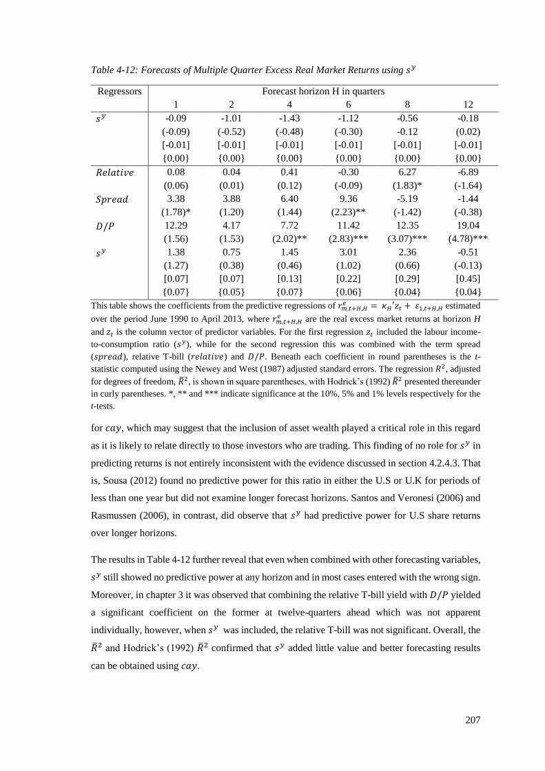
207

Table 4-12: Forecasts of Multiple Quarter Excess Real Market Returns using 𝑠𝑦

Regressors Forecast horizon H in quarters

1 2 4 6 8 12

𝑠𝑦 -0.09

(-0.09)

[-0.01]

{0.00}

-1.01

(-0.52)

[-0.01]

{0.00}

-1.43

(-0.48)

[-0.01]

{0.00}

-1.12

(-0.30)

[-0.01]

{0.00}

-0.56

-0.12

[-0.01]

{0.00}

-0.18

(0.02)

[-0.01]

{0.00}

𝑅𝑒𝑙𝑎𝑡𝑖𝑣𝑒

𝑆𝑝𝑟𝑒𝑎𝑑

𝐷/𝑃

𝑠𝑦

0.08

(0.06)

3.38

(1.78)*

12.29

(1.56)

1.38

(1.27)

[0.07]

{0.07}

0.04

(0.01)

3.88

(1.20)

4.17

(1.53)

0.75

(0.38)

[0.07]

{0.05}

0.41

(0.12)

6.40

(1.44)

7.72

(2.02)**

1.45

(0.46)

[0.13]

{0.07}

-0.30

(-0.09)

9.36

(2.23)**

11.42

(2.83)***

3.01

(1.02)

[0.22]

{0.06}

6.27

(1.83)*

-5.19

(-1.42)

12.35

(3.07)***

2.36

(0.66)

[0.29]

{0.04}

-6.89

(-1.64)

-1.44

(-0.38)

19.04

(4.78)***

-0.51

(-0.13)

[0.45]

{0.04}



and 𝑧𝑡 is the column vector of predictor variables. For the first regression 𝑧𝑡 included the labour income-

to-consumption ratio (𝑠𝑦), while for the second regression this was combined with the term spread

(𝑠𝑝𝑟𝑒𝑎𝑑), relative T-bill (𝑟𝑒𝑙𝑎𝑡𝑖𝑣𝑒) and 𝐷/𝑃. Beneath each coefficient in round parentheses is the t-

statistic computed using the Newey and West (1987) adjusted standard errors. The regression 𝑅2, adjusted

for degrees of freedom, ��2, is shown in square parentheses, with Hodrick’s (1992) ��2 presented thereunder

in curly parentheses. *, ** and *** indicate significance at the 10%, 5% and 1% levels respectively for the

t-tests.

for 𝑐𝑎𝑦, which may suggest that the inclusion of asset wealth played a critical role in this regard

as it is likely to relate directly to those investors who are trading. This finding of no role for 𝑠𝑦 in

predicting returns is not entirely inconsistent with the evidence discussed in section 4.2.4.3. That

is, Sousa (2012) found no predictive power for this ratio in either the U.S or U.K for periods of

less than one year but did not examine longer forecast horizons. Santos and Veronesi (2006) and

Rasmussen (2006), in contrast, did observe that 𝑠𝑦 had predictive power for U.S share returns

over longer horizons.

The results in Table 4-12 further reveal that even when combined with other forecasting variables,

𝑠𝑦 still showed no predictive power at any horizon and in most cases entered with the wrong sign.

Moreover, in chapter 3 it was observed that combining the relative T-bill yield with 𝐷/𝑃 yielded

a significant coefficient on the former at twelve-quarters ahead which was not apparent

individually, however, when 𝑠𝑦 was included, the relative T-bill was not significant. Overall, the

��2 and Hodrick’s (1992) ��2 confirmed that 𝑠𝑦 added little value and better forecasting results

can be obtained using 𝑐𝑎𝑦.

208

4.4.3.2 Cross-sectional Regression Results

The correlation coefficients between the pricing factors in the three conditional models examined

with 𝑠𝑦, as shown in Table C-5 in the appendix (p. 331), were relatively low and thus, it was not

considered necessary to orthogonalise any of the pricing factors. The cross-sectional results for

the three conditional models are depicted in Table 4-13. The ��2 estimate for the conditional

CAPM with labour income of 47% mirrors that documented by Santos and Veronesi (2006) for

the U.S of 48% and exceeds the 35% obtained by Li et al. (2011) for Australia. In Santos and

Veronesi’s (2006) results only the scaled market risk premium was significant whereas Li et al.

(2011) found only the time-varying intercept was significant. In this study however, while the

scaled market risk premium and the market risk premium were priced, they both entered with the

wrong sign (a similar finding to other models in this study); therefore suggesting in fact that

judging the model’s performance based only on R2 is inappropriate. The same is thus true in

comparing this specification to the conditional models using cay in the previous section, with the

latter achieving a lower R2 but the signs of the pricing factors were more consistent with theory

than is the case with these models. Thus, this model had little success in explaining the size and

value anomalies on the JSE. The role of labour income in pricing the cross-section of South

African security returns is clearly not salvaged by allowing for time-variation in the risk measure

as indicated by the insignificant pricing factor. Further proof of this is evident in reviewing the

explanatory power of the conditional CAPM with sy which was actually higher (53% compared

to 47%) when labour income was excluded. The other results pertaining to the significance of the

market risk premium and scaled market risk premium but with the incorrect sign were also true

for the model excluding labour income.

Although the coefficient on the time-varying intercept was insignificant, the sy betas for the 16

size and value portfolios were briefly examined, as shown in Figure 4-10. As Li et al. (2011)

highlighted, these betas should be negative given that sy is expected to have a negative

relationship with future returns. Nine of the portfolios did exhibit negative betas with these

principally occurring on the value portfolios rather than the growth portfolios. This suggests that

value shares necessitated a high risk premium because they moved closely with future movements

in the business cycle, whereas growth shares do not as they effectively act as a hedge. Such a

relationship should therefore give rise to a negative risk premium in the cross-sectional

regressions. However, as the results in Table 4-13 indicate, this is not the case (as was true for the

Australian market) with the principle cause of this being that the small shares exhibited significant

positive 𝑠𝑦 betas while the large shares had negative betas. Thus, although there was anecdotal

evidence that 𝑠𝑦 may be able to explain some of the value anomaly, the relationship observed

across the size portfolios effectively negated this explanatory power. The pricing errors from this

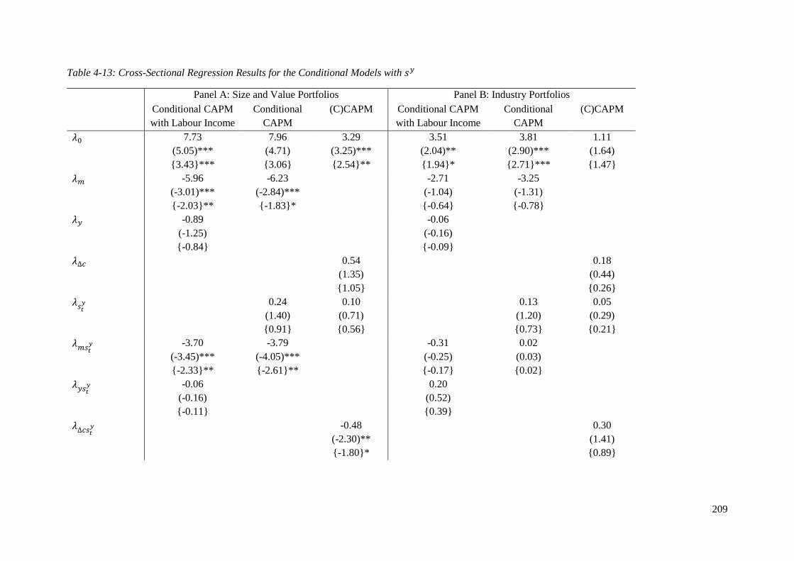
209

Table 4-13: Cross-Sectional Regression Results for the Conditional Models with 𝑠𝑦


Conditional CAPM

with Labour Income

Conditional

CAPM

(C)CAPM Conditional CAPM

with Labour Income

Conditional

CAPM

(C)CAPM

𝜆0 7.73

(5.05)***

{3.43}***

7.96

(4.71)

{3.06}

3.29

(3.25)***

{2.54}**

3.51

(2.04)**

{1.94}*

3.81

(2.90)***

{2.71}***

1.11

(1.64)

{1.47}

𝜆𝑚 -5.96

(-3.01)***

{-2.03}**

-6.23

(-2.84)***

{-1.83}*

-2.71

(-1.04)

{-0.64}

-3.25

(-1.31)

{-0.78}

𝜆𝑦 -0.89

(-1.25)

{-0.84}

-0.06

(-0.16)

{-0.09}

𝜆∆𝑐 0.54

(1.35)

{1.05}

0.18

(0.44)

{0.26}

𝜆𝑠𝑡𝑦 0.24

(1.40)

{0.91}

0.10

(0.71)

{0.56}

0.13

(1.20)

{0.73}

0.05

(0.29)

{0.21}

𝜆𝑚𝑠𝑡𝑦 -3.70

(-3.45)***

{-2.33}**

-3.79

(-4.05)***

{-2.61}**

-0.31

(-0.25)

{-0.17}

0.02

(0.03)

{0.02}

𝜆𝑦𝑠𝑡𝑦 -0.06

(-0.16)

{-0.11}

0.20

(0.52)

{0.39}

𝜆∆𝑐𝑠𝑡𝑦 -0.48

(-2.30)**

{-1.80}*

0.30

(1.41)

{0.89}

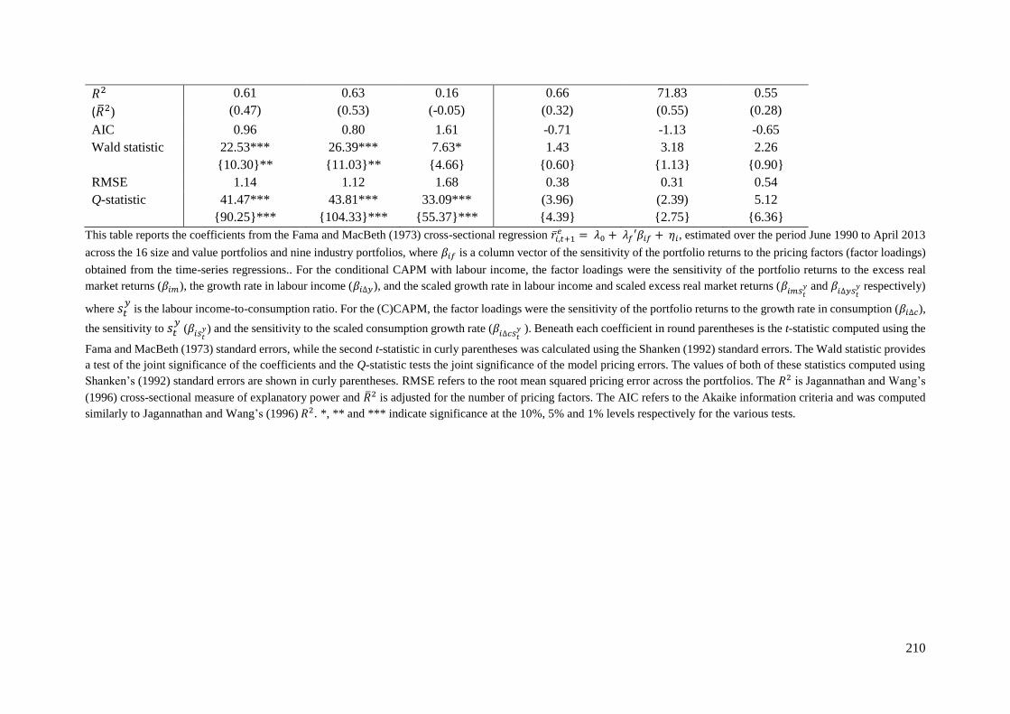
210

𝑅2

(��2)

0.61

(0.47)

0.63

(0.53)

0.16

(-0.05)

0.66

(0.32)

71.83

(0.55)

0.55

(0.28)

AIC 0.96 0.80 1.61 -0.71 -1.13 -0.65


{10.30}**

26.39***

{11.03}**

7.63*

{4.66}

1.43

{0.60}

3.18

{1.13}

2.26

{0.90}

RMSE 1.14 1.12 1.68 0.38 0.31 0.54


{90.25}***

43.81***

{104.33}***

33.09***

{55.37}***

(3.96)

{4.39}

(2.39)

{2.75}

5.12

{6.36}


across the 16 size and value portfolios and nine industry portfolios, where 𝛽𝑖𝑓 is a column vector of the sensitivity of the portfolio returns to the pricing factors (factor loadings)

obtained from the time-series regressions.. For the conditional CAPM with labour income, the factor loadings were the sensitivity of the portfolio returns to the excess real

market returns (𝛽𝑖𝑚), the growth rate in labour income (𝛽𝑖∆𝑦), and the scaled growth rate in labour income and scaled excess real market returns (𝛽𝑖𝑚𝑠𝑡𝑦 and 𝛽𝑖∆𝑦𝑠𝑡

𝑦 respectively)

where 𝑠𝑡𝑦

is the labour income-to-consumption ratio. For the (C)CAPM, the factor loadings were the sensitivity of the portfolio returns to the growth rate in consumption (𝛽𝑖∆𝑐),

the sensitivity to 𝑠𝑡𝑦

(𝛽𝑖𝑠𝑡𝑦) and the sensitivity to the scaled consumption growth rate (𝛽𝑖∆𝑐𝑠𝑡

𝑦 ). Beneath each coefficient in round parentheses is the t-statistic computed using the

Fama and MacBeth (1973) standard errors, while the second t-statistic in curly parentheses was calculated using the Shanken (1992) standard errors. The Wald statistic provides

a test of the joint significance of the coefficients and the Q-statistic tests the joint significance of the model pricing errors. The values of both of these statistics computed using

Shanken’s (1992) standard errors are shown in curly parentheses. RMSE refers to the root mean squared pricing error across the portfolios. The 𝑅2 is Jagannathan and Wang’s

(1996) cross-sectional measure of explanatory power and ��2 is adjusted for the number of pricing factors. The AIC refers to the Akaike information criteria and was computed

similarly to Jagannathan and Wang’s (1996) 𝑅2. *, ** and *** indicate significance at the 10%, 5% and 1% levels respectively for the various tests.

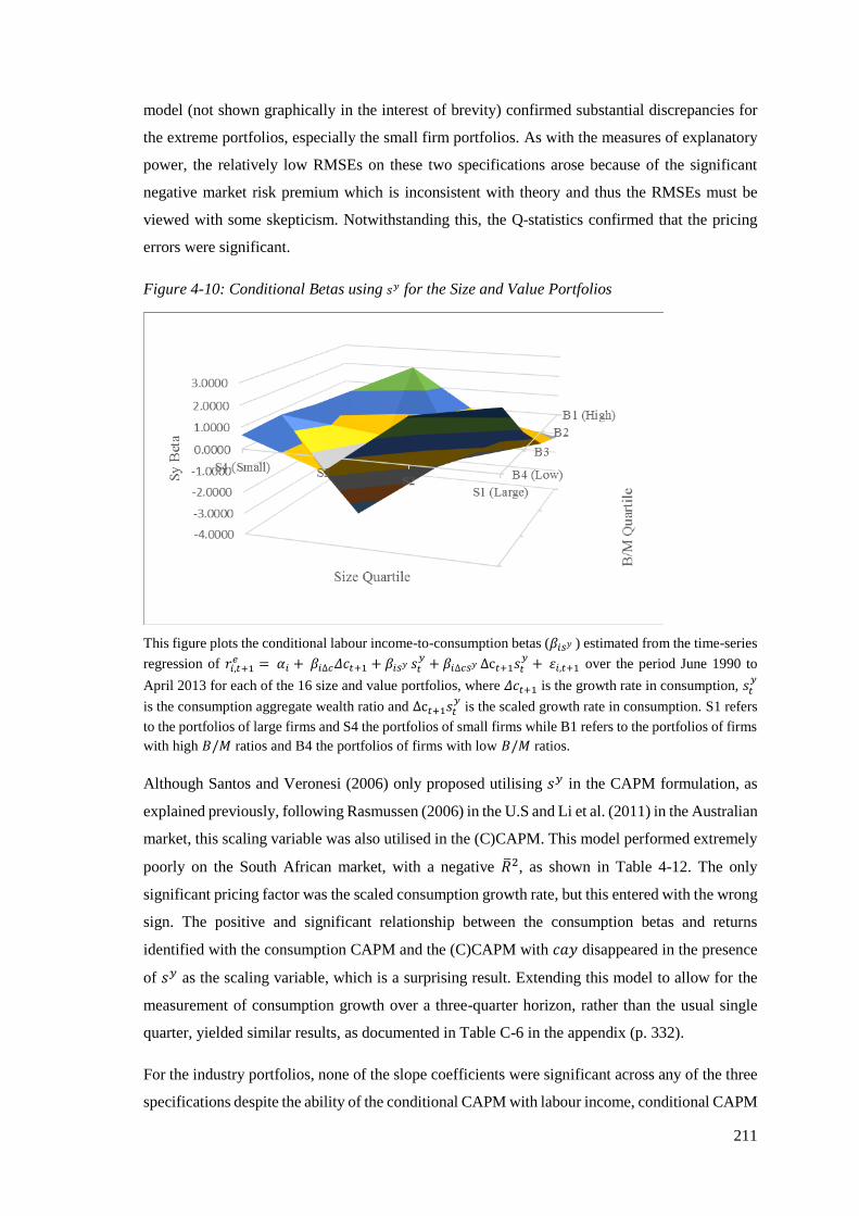
211

model (not shown graphically in the interest of brevity) confirmed substantial discrepancies for

the extreme portfolios, especially the small firm portfolios. As with the measures of explanatory

power, the relatively low RMSEs on these two specifications arose because of the significant

negative market risk premium which is inconsistent with theory and thus the RMSEs must be

viewed with some skepticism. Notwithstanding this, the Q-statistics confirmed that the pricing

errors were significant.

Figure 4-10: Conditional Betas using 𝑠𝑦 for the Size and Value Portfolios

This figure plots the conditional labour income-to-consumption betas (𝛽𝑖𝑠𝑦 ) estimated from the time-series

regression of 𝑟𝑖,𝑡+1𝑒 = 𝛼𝑖 + 𝛽𝑖∆𝑐𝛥𝑐𝑡+1 + 𝛽𝑖𝑠𝑦 𝑠𝑡

𝑦+ 𝛽𝑖∆𝑐𝑠𝑦 Δc𝑡+1𝑠𝑡

𝑦+ 휀𝑖,𝑡+1 over the period June 1990 to

April 2013 for each of the 16 size and value portfolios, where 𝛥𝑐𝑡+1 is the growth rate in consumption, 𝑠𝑡𝑦

is the consumption aggregate wealth ratio and Δc𝑡+1𝑠𝑡𝑦

is the scaled growth rate in consumption. S1 refers



Although Santos and Veronesi (2006) only proposed utilising 𝑠𝑦 in the CAPM formulation, as

explained previously, following Rasmussen (2006) in the U.S and Li et al. (2011) in the Australian

market, this scaling variable was also utilised in the (C)CAPM. This model performed extremely

poorly on the South African market, with a negative ��2, as shown in Table 4-12. The only

significant pricing factor was the scaled consumption growth rate, but this entered with the wrong

sign. The positive and significant relationship between the consumption betas and returns

identified with the consumption CAPM and the (C)CAPM with 𝑐𝑎𝑦 disappeared in the presence

of 𝑠𝑦 as the scaling variable, which is a surprising result. Extending this model to allow for the

measurement of consumption growth over a three-quarter horizon, rather than the usual single

quarter, yielded similar results, as documented in Table C-6 in the appendix (p. 332).

For the industry portfolios, none of the slope coefficients were significant across any of the three

specifications despite the ability of the conditional CAPM with labour income, conditional CAPM

212

and (C)CAPM to explain 32%, 55% and 28% of the variation respectively, and the insignificant

pricing errors. However, as mentioned previously the latter observations appear to be attributable

more to the lack of variation across the industry-allocated portfolios than the goodness of fit of

the models. This conclusion is consistent with Li et al.’s (2011) observations for the Australian

market. This is of particular interest given that they found Santos and Veronesi’s (2006) model to

have some success in explaining returns of the size- and value-sorted portfolios but the model

could not explain patterns in industry-sorted portfolios.


The final analysis of the models of Santos and Veronesi (2006) was conducted in the GMM

framework, with the results shown in Table 4-14. For the conditional CAPM with labour income

on the size and value portfolios, the labour beta was significant but, as was the case with the

CAPM with labour income examined in section 4.4.1.2, the risk premium was negative, which is

inconsistent with the theoretical paradigm. The scaled labour risk premium was insignificant. In

this model and the conditional CAPM without labour income, the scaled market risk premia were

significant, but similarly to the cross-sectional results, the coefficients were negative. The

unscaled market risk premia were also negative in both models, although only significant in the

specification without labour income.

Turning to the (C)CAPM, the risk premium on the consumption beta was positive and significant,

which was not the case in the cross-sectional results, while neither the time-varying intercept or

slope coefficient were significant. Overall, none of these specifications were able to explain the

pricing errors associated with these portfolios, as signalled by the significant J-statistics.

Moreover, given the limitations of the J-statistic, as highlighted in section 2.4.3, it was not

possible to compare the errors under each model based on this statistic because they are model

specific.

The GMM regressions for the industry portfolios yielded no significant pricing factors in either

the SDF or linear factor model; consistent with the results from the cross-sectional regressions

that the conditional CAPM with labour income, conditional CAPM and (C)CAPM with 𝑠𝑦 could

not explain the patterns in returns across these portfolios. The insignificant J-statistics thus simply

indicated that the pricing errors for these portfolios were small rather as a consequence of a good

fitting asset pricing model.

Overall, these results are thus largely identical to those from the cross-sectional tests and point to

the inability of the conditional CAPM, conditional CAPM with labour income and (C)CAPM

with 𝑠𝑦 to explain returns to portfolios sorted both on firm characteristics (size and the 𝐵/𝑀 ratio)

and industry-affiliations.

213

Table 4-14: GMM Regression Results for the Conditional Models with 𝑠𝑦


Conditional CAPM with

Labour Income

Conditional CAPM (C)CAPM Conditional CAPM with

Labour Income

Conditional CAPM (C)CAPM

𝑏𝑚 0.02

(0.87)

0.05**

(2.26)

0.02

(0.94)

0.01

(0.77)

𝑏∆𝑦 0.54**

(2.56)

-0.09

(-0.35)

𝑏∆𝑐 0.60***

(5.77)

0.39

(1.39)

𝑏𝑠𝑡𝑦 0.06

(0.06)

-0.22

(-0.30)

-0.43

(-0.38)

0.20

(0.16)

𝑏𝑚𝑠𝑡𝑦 0.16**

(2.49)

0.23***

(3.07)

0.13

(1.16)

-0.11

(-1.43)

𝑏𝑦𝑠𝑡𝑦 -0.32

(-0.89)

-0.27

(-0.45)

𝑏∆𝑐𝑠𝑡𝑦 0.12

(0.32)

-0.60

(-0.98)

J-Statistic 33.22*** 66.46*** 28.02*** 3.06 3.91 6.19

𝜆𝑚 -1.50

(-0.88)

-4.77**

(-2.29)

-2.09

(-0.95)

-1.04

(-0.76)

𝜆∆𝑦 -1.57**

(-2.62)

0.26

(1.41)

𝜆∆𝑐 1.41***

(5.85)

-0.93

(-1.41)

𝜆𝑠𝑡𝑦 -0.01

(-0.06)

-0.04

(-0.33)

0.07

(0.38)

-0.03

(-0.15)

𝜆𝑚𝑠𝑡𝑦 -2.44** -3.57*** -1.93 1.70

214

(-2.52) (-3.42) (-1.17) (1.42)

𝜆∆𝑦𝑠𝑡𝑦 0.27

(-0.03)

0.23

(0.45)

𝜆∆𝑐𝑠𝑡𝑦 -0.06

(-0.07)

0.31

(1.00)

This table shows the coefficients from Hansen’s (1982) optimal two-stage GMM estimation of the SDF 𝑚𝑡+1 = 𝛼 + 𝑏′𝑓𝑡+1, where 𝑚𝑡+1 is the SDF, 𝑓𝑡+1 is a column vector of

the pricing factors and 𝛼 was normalised to one. For the conditional CAPM with labour income 𝑓𝑡+1 included the includes the excess market returns (𝑟𝑚,𝑡+1𝑒 ), the growth rate in

labour income (∆𝑦𝑡+1), the conditioning variable – the labour income-to-consumption ratio (𝑠𝑡𝑦

) –, the scaled excess market returns (𝑟𝑚,𝑡+1𝑒 𝑠𝑡

𝑦) and the scaled growth rate in

labour income (∆𝑦𝑡+1𝑠𝑡𝑦

). The conditional CAPM included the same factors as the conditional CAPM with labour income but without the two terms capturing the growth rate

in labour income, while for the (C)CAPM, the factors were the growth rate in consumption (∆𝑐𝑡+1), 𝑠𝑡𝑦

and the scaled consumption growth rate (∆𝑐𝑡+1𝑠𝑡𝑦

). The models were

estimated for the size and value portfolios and the industry portfolios. The transformed risk premia (𝜆) are presented in the bottom half of the table and were computed from the

SDF coefficients as 𝜆 = −𝑣𝑎𝑟(𝑓)𝑏, where 𝑣𝑎𝑟(𝑓) is the variance of the pricing factor. Beneath both the 𝑏’s and 𝜆’s the t-statistics are displayed in round parentheses, with the

standard errors of the transformed 𝜆’s computed using the delta method. Hansen’s (1982) J-statistic for the test of the pricing errors is also shown. *, ** and *** indicate

significance at the 10%, 5% and 1% levels respectively.

215

4.4 CONCLUSION

Labour income is closely linked to consumption as it affects the ability of an individual to

consume goods and services in the current and following periods as investors seek to maintain a

constant level of consumption. In turn, this affects the utility investors derive from investments

such that labour income can be seen to play a critical role in linking consumption and asset returns.

The consumption CAPM should incorporate the risk arising from labour income but because

proxies for consumption are used they may not provide an accurate reflection thereof and in

addition, this model does not account for the possibility that risk and returns may vary over

business cycles. The models of Lettau and Ludvigson (2001b) and Santos and Veronesi (2006)

deal with both of these issues by using measures that link consumption and labour income (and

can predict share returns) into the conditional CAPM and consumption CAPM. These models

have been found to have substantial success on international markets in explaining the size and

value anomalies. These models were thus tested on the JSE to assess their ability to explain the

cross-section of share returns.

Directly evaluating the role of labour income as a priced factor in the CAPM provides a more

comprehensive measure of total wealth and thus can be seen as a direct response to Roll’s (1977)

critique of the model. While the CAPM was seen to be a very limited model theoretically in

chapter 2, the premise that total wealth is a key determinant of consumption ties this model to the

consumption framework and is thus frequently seen as a means of practically implementing the

consumption CAPM (Lustig & van Nieuwerburgh, 2008; Bansal et al., 2014). Thus, in addition

to the models of Lettau and Ludvigson (2001b) and Santos and Veronesi (2006), the CAPM

augmented with labour income was also tested.

The CAPM with labour income and (C)CAPM were found to offer no additional insight in pricing

securities as labour income was either not priced in the cross-section, or, where it was, it was

found to have a negative sign inconsistent with intuition that shares which are more highly

correlated with labour income should earn a higher return. When comparing this finding to that

obtained internationally, it was found that the developing market of South Africa was not

noticeably different as labour income was not found to be priced in Australia or the U.K, with

mixed evidence for the U.S as well. The Japanese market, where the premium on small shares

was found to be a consequence of their high correlation with labour income, thus appeared to be

the exception. Similarly poor results were obtained when the labour income-to-consumption ratio

(𝑠𝑦) of Santos and Veronesi (2006) was used to scale returns in the conditional CAPM and

(C)CAPM. However, the model of Lettau and Ludvigson (2001b), which uses the aggregate

wealth ratio (𝑐𝑎𝑦), was found to have some explanatory power for the South African market, with

weak evidence to suggest that value shares earned more because they were riskier during bad

216

states when 𝑐𝑎𝑦 was high. But this model was not able to explain all of the patterns in the returns,

with the pricing errors remaining significant and both SMB and HML still priced in returns.

Although Lettau and Ludvigson (2001b) found the (C)CAPM to be extremely successful in

accounting for the anomalies in the U.S market, the South African evidence is more closely

aligned to that observed for Australia and the U.K, where the model was able to explain some but

not all of the cross-sectional variation. One of the potential reasons for the differences observed

is that labour income and consumption are measured as aggregate values and thus their correlation

with the share market may not be a true reflection of the way investors, who represent only a

small component of the aggregate in South Africa, view labour income and consumption in their

investment decisions. Moreover, on the JSE investment decisions are dominated by institutional

investors, who although represent individuals, may be less concerned about the co-movement in

share returns and aggregate consumption and labour income than individual investors.

Accordingly, while theory predicts a role for labour income in pricing securities, the evidence for

the South African market was relatively weak. In the following chapter, the role of housing wealth

in pricing securities in the South African market is considered to ascertain whether that factor is

able to explain some of the anomalous patterns in returns observed on this market.

217

Chapter 5 : THE ROLE OF HOUSING WEALTH IN ASSET

PRICING

5.1 INTRODUCTION

An accurate asset pricing model is one where assets which perform poorly during bad times earn

a higher return. However, as Cochrane (2008a, pp. 302) maintains, the difficulty is in identifying

the right measure of bad times. As highlighted in section 3.4, there has been a trend in asset pricing

tests to link bad times to macroeconomic fundamentals, with consumption the most obvious

candidate as it provides information about wealth and income prospects. However, as the

international literature and the results from the study of the South African market revealed, as the

sole pricing factor consumption cannot capture differences in returns across assets. As such, the

consumption CAPM does not provide a suitable asset pricing model. In the previous chapter, the

effects of labour income on consumption and share returns were considered, but labour income

may not provide all the missing information in consumption and thus in this chapter, the principle

focus is the interaction between housing wealth and consumption (and labour income) and the

implications for share returns.

The wealth that an investor holds in housing can be used to fund consumption expenditure on

goods and services, especially given the desire of investors to smooth consumption patterns over

time. In turn, this will affect security prices as those investments which pay out when housing

wealth is low will provide greater marginal utility than those investments which yield high returns

when housing wealth is high. Accordingly, consumption, housing wealth and share returns should

be linked; with evidence to support this documented in several studies including Piazzesi et al.

(2003, 2007), Lustig and van Nieuwerburgh (2005), Bostic, Gabriel, and Painter (2009) and

André, Gupta and Kanda (2012).

Given the shortcomings of the measure of consumption used in the consumption CAPM, as

indicated in the previous chapters, it is plausible that the risk arising from the relationship between

consumption and housing wealth may not be fully incorporated into the asset pricing model. As

a consequence, several scholars have sought to expand the consumption CAPM to account for the

risk of housing wealth and in so doing, consider how the various measures of risk in the model

may vary over time with changes in the business cycle (Piazzesi et al., 2003; Lustig & van

Nieuwerburgh, 2005). The work on the effects of housing wealth on asset pricing, similarly to

that on human capital, originated in the CAPM framework (Kullmann, 2003; Funke et al., 2010)

as a means to provide a more encompassing estimate of the market portfolio rather than that based

218

solely on the returns from ordinary shares. As such, these studies do not directly consider the link

between consumption, housing wealth and share returns, but do provide valuable insight

regarding housing wealth as a risk factor which affects aggregate returns (in an APT-type model).

In this regard, the evidence generally indicates that shares which are more highly correlated with

the returns to housing wealth earn higher returns.

The focus of the analysis in this chapter is to examine whether models that link housing wealth

(and labour income) to consumption can explain differences in returns across shares listed on the

JSE. The remainder of the chapter is laid out as follows: the links between housing wealth,

consumption and share returns are briefly discussed, followed by a review of the theory and

performance of asset pricing models that include housing wealth. Thereafter, several of these

models are tested and the results compared to the international literature and the performance of

the other asset pricing models tested in the preceding chapters.

5.2 HOUSING WEALTH IN ASSET PRICING

5.2.1 The Importance of Housing Wealth

As highlighted in chapter 4, the ability of an individual to consume goods and services in the

current and following periods is affected by human capital. The same is arguably true for housing

wealth, as a higher marginal propensity to consume from housing wealth causes investors to

smooth their spending (Carroll, Otsuka, & Slacalek, 2011). This is related to security prices, as if

returns are low, households can use their wealth from property to increase consumption

(stabilising the economy) while the opposite is true when financial assets provide a higher return.

Bostic et al. (2009) confirmed that there is a strong relationship between housing wealth, financial

wealth and consumption, with André et al. (2012) demonstrating that there is a significant and

positive consumption response to a shock in housing in the U.K, Canada, France and Japan. Gan

(2010) showed that changes in consumption patterns of individual households in Hong Kong were

significantly affected by changes in housing wealth, with the most important reason for this

change being the precautionary savings motive as a higher house price reduced the need for such

savings and thus enabled households to increase consumption.

Capturing the impact of changes in housing wealth on consumption and investment decisions is

complicated by the nature of residential real estate. Housing as a savings vehicle is extremely

illiquid compared to other financial securities because of the huge transaction costs associated

with buying and selling. Thus, investors could market their own home, but they are more likely

to view it as a fixed portion of their portfolio and often will not consider changing homes as part

of their optimal investment strategy; not only because of the substantial transaction costs

219

associated with this (Jensen, 1972a), but also for non-monetary reasons (Elton, Gruber, Brown,

& Goetzmann, 2014, pp. 318). However, while investors may not sell their homes so as to release

capital to fund consumption, they could borrow against the value of their homes to do so. In

addition to the capital gain that residential property provides, housing as an investment product

also provides a flow of housing services, as the homeowner is able to live in the house rather than

renting it and it can thus be seen as a consumption good (Klinkowska, 2009). Investors can thus

also substitute consumption of housing services for non-housing goods and services.

Several scholars have derived measures which attempt to model the dynamics of the consumption-

housing wealth relationship and the implications for share returns. The initial work of Piazzesi et

al. (2003) focused on the services that are derived from housing as opposed to its investment value

and considered the composition risk of consumption on non-housing goods and services relative

to total consumption. Lustig and van Nieuwerburgh (2005) expanded the work of Piazzesi et al.

(2003) by not only considering the flow of services from housing but also the collateral value that

housing wealth and labour income provide to support consumption. Their measure thus

incorporated risk arising from both housing wealth and labour income. Sousa (2010) also

considered both labour income and housing wealth in his measure in which he expanded the

model of Lettau and Ludvigson (2001a), which linked consumption, asset wealth and labour

income, by decomposing asset wealth into financial and housing wealth. These measures which

utilise different components of the multifaceted housing wealth have all been found to have

predictive power for future share returns and thus tie together the housing wealth (and labour

income) and consumption effects on share returns.

Any risk arising from housing wealth should be fully incorporated into the consumption CAPM.

However, as was noted when reviewing labour income, aggregate consumption is not observable

and as such the measures used are subject to limitations and may not provide an accurate

description of total consumption risk. In particular, the model may not adequately capture the risk

arising from housing wealth (and labour income). Given these shortcomings of the consumption

CAPM and the success of the measures that link consumption and housing wealth in predicting

future returns (Piazzesi et al., 2003; Lustig & van Nieuwerburgh, 2005; Santos, 2010), these ratios

have been proposed as conditioning variables in asset pricing models. These ratios thus

incorporate the consumption risk arising from housing wealth and labour income and in so doing

also allow risk and return to vary across business cycles.

As early as Jensen (1972b) and Stambaugh (1982), the need to include wealth arising from

housing into a more comprehensive measure of the market portfolio was acknowledged, as

similarly to human capital wealth, it is ignored when an ordinary share index is used as a proxy

for the market portfolio. This is extremely pertinent as statistics indicate that individuals hold

220

more of their total wealth in housing than financial assets; for example, the 2001 Survey of

Consumer Finances in the U.S, revealed that for the median household, 65% of their wealth was

tied up in the family house with investments in cash, bonds and mutual funds (outside of

retirement savings) only accounting for 23% of total wealth for the average American family

(Benjamin, Chinloy, & Jud, 2004, pp. 329). Thus, it is likely that investors will be concerned

about how closely their shares are correlated with their housing wealth. Accordingly, the inclusion

of housing wealth alongside financial wealth goes some way to addressing Roll’s (1977) critique

of the CAPM (Funke et al., 2010) and as such the initial studies (Kullmann, 2003; Funke et al.,

2010) of the effects of housing wealth on asset pricing have been viewed as extensions to the

traditional CAPM. This research not only provides valuable information about whether investors

consider sensitivity to the returns to housing as a source of risk of a security but also because total

wealth is the key determinant of consumption (as highlighted in section 3.4.1), this asset pricing

model also indirectly links housing wealth to consumption.

5.2.2 The CAPM with Real Estate Wealth

The CAPM-based models which have been expanded to include the effects of housing focus on

the broader category of real estate. Kullmann (2003) incorporated both the key components of

real estate wealth in the form of residential and commercial property, with the former likely to

capture the information pertaining to the returns from an investment in housing. Commercial real

estate, while a potentially important source of wealth for some investors, is likely to be a less

important factor in driving consumption than housing wealth. But, because of the difficulty in

measuring returns to residential real estate (with the measure used ignoring the services

component), and because the measure of commercial real estate (indirect property investments)

also includes some residential property, its use helps to provide a more comprehensive measure

of real estate wealth. In fact, Funke et al. (2010) only used the returns to commercial property as

their measure of real estate wealth.

Kullmann (2003) assumed that the returns to the market portfolio are a linear function of the

returns to the value-weighted share index and the returns to both residential and commercial real

estate. This yields a three-factor model as follows

𝐸(𝑟𝑖,𝑡+1𝑒 ) = 𝜆0 + 𝜆𝑚𝛽𝑖𝑚 + 𝜆𝑅𝑅𝐸𝛽𝑅𝑅𝐸 + 𝜆𝐶𝑅𝐸𝛽𝐶𝑅𝐸 (5.1)

where 𝑟𝑅𝑅𝐸,𝑡+1𝑒 and 𝑟𝐶𝑅𝐸,𝑡+1

𝑒 measure the excess returns to residential and commercial real estate

respectively and 𝛽𝑅𝑅𝐸 and 𝛽𝐶𝑅𝐸 are the residential and commercial real estate betas which capture

the sensitivity of the share returns to the two factors (Kullmann, 2003, p. 9). These real estate

betas were estimated via a time-series regression of the portfolio returns against the real estate

returns as with other factor loadings. This model is referred to as the real estate augmented CAPM.

221

Following Dybvig and Ingersoll (1982), the linear SDF implied by the real estate augmented

CAPM can be written as follows

𝑚𝑡+1 = 𝛼0 + 𝑏0𝑟𝑚,𝑡+1𝑒 + 𝑏1𝑟𝑅𝑅𝐸,𝑡+1

𝑒 + 𝑏2𝑟𝐶𝑅𝐸,𝑡+1𝑒 . (5.2)

Kullmann (2003) measured the returns to residential real estate as the monthly percentage change

in the median price of homes sold and the returns to commercial real estate as the percentage

change in the equity REIT index. For the initial tests on size- and beta-sorted portfolios, the ��2

increased from 14% for the CAPM to 48% for the real estate CAPM. The market and commercial

real estate risk premia were insignificant, but a positive and significant risk premium on the

residential real estate beta was observed. This positive coefficient indicates that portfolios which

had a greater sensitivity to residential real estate earned a higher return. This finding that

residential real estate is more important than commercial real estate in the cross-section of returns

is largely consistent with earlier work of Cochrane (1996), who found that his measure of

residential investment, which included real estate as a major component was more important to

investors than non-residential investment (which incorporated commercial real estate).

The finding of an insignificant market risk premium contrasts with the early study of Stambaugh

(1982). As mentioned in section 2.3.3, Stambaugh (1982) identified a positive market risk

premium when the market portfolio returns were computed only using those from an ordinary

share index as well as when the market portfolio returns also included a weighting in real estate.

Thus, his results not only showed no support for the role of real estate in asset pricing but also

that the CAPM provided a reasonably accurate description of the differences in returns. However,

his use of industry-sorted portfolios rather than those sorted based on firm characteristics may

account for some of the differences observed. More recently, however, Klinkowska (2009)

included human capital and housing wealth in the market portfolio and found that the use of a

more representative market portfolio improved the explanatory power of the model substantially,

with the size and value premia smaller, although still present.

Kullmann (2003) also extended the real estate CAPM to allow for time-variation in returns, with

the T-bill used as the conditioning variable, but this yielded only a marginal increase in the ��2

from 45% to 51%, with residential real estate again significant while commercial real estate was

not. Interestingly, in this specification, the market risk premium was priced, but it entered with

the wrong sign. Although Kullmann (2003) found the risk premium on labour income to be

positive and significant in testing the CAPM with labour income, when combined with the real

estate factors it was not priced and added no additional explanatory power. This suggests that real

estate risk subsumes the effects of labour income risk in the cross-section of U.S share returns.

222

In tests of the 25 size and value portfolios, Kullmann (2003) obtained some contrasting results,

as rather than the residential real estate risk premium being significant, that on commercial

property was significant (and positive) showing that the latter appeared to be more important in

accounting for the value effect. When size and value were included in the specification, neither

factor was significant; however, the importance of the real estate factors was reduced.

Funke et al. (2010) also evaluated the ability of the real estate CAPM to explain the returns on

the 25 size- and value-sorted portfolios but, as mentioned, only included the commercial real

estate returns. Similarly to Kullmann’s (2003) findings for these portfolios, the coefficient on the

real estate factor was significant and positive while the market risk premium was not. An analysis

of the portfolio loadings on the real estate factor from the time-series regressions indicated that

they increased monotonically from lower to higher B/M quintiles; with the opposite pattern on

the size portfolios. The model was able to account for 77% of the variation in the returns across

the 25 portfolios, approximately equivalent to the three-factor model with 75% (Funke et al.,

2010). While neither the real estate augmented CAPM nor the three-factor model satisfied the

requirements of zero pricing errors, the former was better able to explain the returns associated

with the large value portfolios than the three-factor model. However, the model was less

successful in accounting for the size anomaly. Finally, Funke et al. (2010) also documented that

real estate risk was a unique risk not captured by other risk factors which have been found to be

able to explain some of the anomalous returns to the size and value portfolios such as the default

and term spreads, GDP growth or distress risk.

The finding that commercial real estate could explain some of the differences in returns across

the value and growth shares in both of these two studies is consistent with the rationale of Hsieh

and Peterson (2000) that if real estate represents a substantial component of the book value of

assets, then a systematic real estate risk measure may capture the value anomaly. Gan (2007a,

2007b) documented similar linkages between real estate risk and returns through collateral and

lending channels. Accordingly, these results speak to the impact of real estate being more closely

influenced by corporate risk than through consumption and as such, provide a link to production-

based asset pricing models rather than the consumption-based models which examine the

relationship between housing wealth and consumption. These models fall beyond the scope of

this study but the link thereof to the findings of this analysis are examined in chapter 6.

223

5.2.3 Conditional Models with Scaling Factors that Include Housing Wealth64

5.2.3.1 Piazzesi et al. (2003, 2007)

As discussed in section 5.2.1, consumption, housing wealth and security returns should be related.

Piazzesi et al. (2007) were amongst the first authors to derive a measure to capture this

relationship. In their model they focused on the services derived from housing as opposed to the

value of the capital. Piazzesi et al. (2007, p. 537) disaggregated total consumption into two non-

separable components - consumption on housing services (ℎ𝑡) and non-housing services (𝑛ℎ𝑡)65

and used the following constant elasticity of consumption utility function

𝑈(𝑛ℎ𝑡, ℎ𝑡) = (𝑛ℎ𝑡(𝜀−1)/𝜀

+ 𝜔ℎ𝑡(𝜀−1)/𝜀

)(𝜀−1)/𝜀, (5.3)

where 휀 is the intratemporal elasticity of substitution between consumption of housing services

and non-housing services. High values of 휀 mean that agents will readily substitute between the

two goods within a period. An important component of the model is the share of total expenditure

on non-housing consumption, denoted 𝛼, which is defined as the proportion of total consumption

spent on non-housing services 𝛼𝑡 = 𝑛ℎ𝑡/𝑐𝑡.

In the consumption CAPM, the SDF was defined as 𝑚𝑡+1 = 𝜃(𝐶𝑡+1

𝐶𝑡)−𝛾, which could be rewritten

as 𝑚𝑡+1 = 𝜃(𝐶𝑡+1

𝐶𝑡)−1/𝜎 so as to reflect the intertemporal elasticity of substitution as opposed to

the parameter of relative risk aversion. Substituting the utility function of 5.3 into this pricing

kernel (and simplifying by including the expenditure share) yields

𝑚𝑡+1 = 𝜃(𝑛ℎ𝑡+1

𝑛ℎ𝑡)−1/𝜎 (

𝛼𝑡+1

𝛼𝑡)

(𝜀−𝜎)/(𝜎(𝜀−1)), (5.4)

(Piazzesi et al., 2007, p. 538). This pricing kernel consists of two components. The first is the

standard one good model with power utility, which measures the uncertainty that the agent faces

regarding future levels of non-housing consumption that will be possible (consumption risk). The

second component captures the agent’s concern with composition risk in so far as the uncertainty

associated with the choice between housing and other goods and services that will be possible

(Piazzesi et al., 2007). If ε > σ then agents are more willing to substitute between housing and

non-housing consumption within a period than they are to substitute total consumption across

periods. This is the condition Piazzesi et al. (2007) impose.

64 The ordering of discussion of the papers in this section reflects the fact that the working paper of Piazzesi

et al. (2003) was published before than of Lustig and van Nieuwerburgh (2005). 65 As Cochrane (2008a, pp. 279) states, an individual cannot watch television without having a roof!

224

The pricing kernel in 5.4 indicates that non-housing consumption is valued when it is expected to

be lower in the following period compared to the current period. In addition, this model shows

that non-housing consumption is also valued when the relative consumption of housing services

is lower in the following period than in the current period (Piazzesi et al., 2007). Accordingly,

non-housing consumption is valued not only in a recession (when consumption levels are low)

but even more so in a severe recession, when the relative quantity of housing consumption is low

(Piazzesi et al., 2007). The marginal utility of an extra unit of non-housing consumption is thus

high for severe recessions, because the agent wants to compensate for the future shortfall in

housing services by substituting non-housing consumption. Thus, a security which pays out a lot

when there is a relative shortfall in housing will be highly valued (Cochrane, 2008a, pp. 278).

This housing collateral model thus not only relies on the first term in the SDF to generate higher

returns, but also includes a positive composition effect which increases the risk premium beyond

that implied by the standard consumption CAPM (Piazzesi et al., 2007). As such, expected returns

are high because investors are concerned that shares will payoff less when there is a relative

shortfall in housing during recessions.

This link between share returns and the composition of consumption raises the possibility that α

may be able to forecast returns, with Piazzesi et al. (2007) conducting a series of predictive

regressions, similar to those outlined in chapter 3, for this purpose. The results confirmed a

significant relationship between 𝛼 and share returns, with the positive coefficient consistent with

the theoretical framework that 𝛼 should be high during a recession when expected returns are

high to compensate investors for the higher risk associated with the composition of their

consumption. The ��2 values from the regressions indicate that 𝛼 was better able to predict returns

over longer horizons of three- to five-years (��2 estimates ranging between 14% to 22%) compared

to returns one- and two-years ahead (��2 values of 2% and 7% respectively). Moreover, this ratio

performed slightly better than 𝐷/𝑃 at all horizons, which was analysed for comparative purposes.

Rasmussen (2006)66 also considered the forecasting power of 𝛼 in her study of the U.S market,

but found little supporting evidence, with the results sensitive to the sample period examined and

the frequency of the data. For those sample periods where predictability was identified, this only

occurred at horizons of over two years using quarterly data and eight years using annual data.

Sousa (2012), however, documented more favourable evidence of the predictive power of 𝛼, as it

was able to forecast returns in the U.S three to four-quarters ahead, and for one- to four-quarters

ahead in the U.K, although the explanatory power of these regressions was relatively low ranging

between 1% and 4%.

66 Rasmussen (2006) utilised the working paper of Piazzesi et al. (2003) as her reference point.

225

Although Piazzesi et al. (2007) did not test the ability of their model to explain cross-sectional

variation in share returns, in their 2003 working paper they did derive a specification for this

purpose, which was used by Lustig and van Nieuwerburgh (2005). For this purpose, Piazzesi et

al. (2003, pp. 20) linearised the pricing kernel in equation 5.4 around the point (𝛥𝑛ℎ𝑡+1, 𝛼𝑡+1) =

(0, 𝛼𝑡), which yields the following approximation

𝑚𝑡+1 ≈ 𝜃exp (1 −1

𝜎(Δ𝑛ℎ𝑡+1) +

𝜀−𝜎

𝜎(𝜀−1)Δ𝛼𝑡+1), (5.5)

where 𝑒𝑥𝑝 refers to the natural exponent 𝑒. Substituting this SDF into the asset pricing framework

and simplifying gives rise to the collateral-housing CAPM (CH-CAPM) in the expected return-

beta framework

𝐸(𝑟𝑖,𝑡+1𝑒 ) = 𝜆0 + 𝜆Δ𝑛ℎ𝛽𝑖Δ𝑛ℎ + 𝜆𝛥𝛼𝛽𝑖Δα, (5.6)

where 𝛽𝑖Δ𝑛ℎ and 𝛽𝑖Δα measure the sensitivity of the portfolio returns to growth in non-housing

consumption and the change in the expenditure share respectively (Piazzesi et al., 2003, p. 30).

Following Dybvig and Ingersoll (1982), the SDF for this equation can be written as67

𝑚𝑡+1 = 𝑏0 + 𝑏1∆𝑛ℎ𝑡+1 + 𝑏2∆𝛼𝑡+1. (5.7)

Piazzesi et al. (2003, p. 30) also presented a (C)CAPM of the form

𝐸(𝑟𝑖,𝑡+1𝑒 ) = 𝜆0 + 𝜆α𝛽iα + 𝜆Δ𝑛ℎ𝛽𝑖Δ𝑛ℎ + 𝜆Δ𝑛ℎ𝛼𝛽𝑖Δ𝑛ℎα, (5.8)

where 𝛼 is the conditioning variable such that 𝛽iα and 𝛽𝑖Δ𝑛ℎα represent the time-varying intercept

and slope coefficients respectively. The SDF implied from this linear factor model is given as

𝑚𝑡+1 = 𝑏0 + 𝑏1𝛼𝑡 + 𝑏2∆𝑛ℎ𝑡+1 + 𝑏3𝛼𝑡∆𝑛ℎ𝑡+1. (5.9)

Finally, Piazzesi et al. (2003, p. 30) combined these two specifications, yielding

𝐸(𝑟𝑖,𝑡+1𝑒 ) = 𝜆0 + 𝜆α𝛽α + 𝜆Δ𝑛ℎ𝛽𝑖Δ𝑛ℎ + 𝜆Δ𝑛ℎ𝛼𝛽𝑖Δ𝑛ℎα + 𝜆𝛥𝛼𝛽𝑖Δα + 𝜆𝛥𝛼𝛼𝛽𝑖Δα𝛼, (5.10)

which they termed the conditional CH-CAPM. The SDF for this model is

𝑚𝑡+1 = 𝑏0 + 𝑏1𝛼𝑡 + 𝑏2∆𝑛ℎ𝑡+1 + 𝑏3𝛼𝑡∆𝑛ℎ𝑡+1 + 𝑏4∆𝛼𝑡+1 + 𝑏5∆𝛼𝑡+1𝛼𝑡. (5.11)

In tests of these models, Piazzesi et al. (2003) found that the models were able to explain 69%,

63% and 78% of the variation across the size- and value-sorted portfolios respectively. This

67 Rather than denoting the static and time-varying intercepts by 𝛼0 and 𝛼1 in the SDF, as was the case in

previous specifications, 𝑏0 and 𝑏1 are used so as to avoid confusion given the definition of 𝛼 as the

expenditure share in these models.

226

explanatory power was only marginally lower than the Fama and French (1993) model achieved

of 84%. The relatively high explanatory power of these models, however, must be interpreted

with some caution, because, as documented in section 3.4.2, the sample period used by Piazzesi

et al. (2003) has been noted to have greater explanatory power for the consumption CAPM than

other periods in U.S history, with the fact that they obtained an ��2 of 56% for the consumption

CAPM compared to the 13% of Lettau and Ludvigson (2001b) evidence of this. This inflation of

the explanatory power of these models as a consequence of the time period chosen was confirmed

by Lustig and van Nieuwerburgh (2005), as when they tested the CH-CAPM, over a longer period

that included the Great Depression, they only obtained an ��2 of 32%. Rasmussen (2006), in a test

of Piazzesi et al.’s (2003) (C)CAPM, also obtained a much lower R2 of between 23 and 28%

depending on the sample period.

Apart from consumption growth, the models of Piazzesi et al. (2003) did reveal a significant role

for 𝛼 in pricing securities. Lustig and van Nieuwerburgh (2005) also found the change in 𝛼 to be

a significant explanatory variable. In the (C)CAPM, the time-varying intercept rather than the

time-varying beta was significant, with the positive coefficient confirming that portfolios which

were more sensitive to a recession (when 𝛼 was high) earned a higher return. However, in the

conditional CH-CAPM, which was able to explain a larger component of the cross-sectional

variation than the (C)CAPM, this time-varying intercept was not significant.

5.2.3.2 Lustig and van Nieuwerburgh (2005)

In the model of Lustig and van Nieuwerburgh (2005) there are two means by which shocks in the

housing market are transmitted to security risk premia. The first follows Piazzesi et al. (2007) in

that consumers wish to hedge against shocks to the composition of their consumption such that,

provided housing services and non-housing services are complements, investors will demand a

higher risk premium if returns and growth in housing services are positively related (Lustig & van

Nieuwerburgh, 2005). Thus securities that are negatively correlated and pay out when housing

services are low are highly valued. Accordingly, Lustig and van Nieuwerburgh (2005) utilised

the utility function given in equation 5.3. However, they contended that the rate of substitution

between current and future consumption is subject to liquidity constraints

𝑚𝑡+1 = 𝑚𝑡+1𝑎 𝑔𝑡+1, (5.12)

where 𝑚𝑡+1𝑎 is the pricing kernel for the representative agent and 𝑔𝑡+1 is the liquidity factor

(Lustig & van Nieuwerburgh, 2005, p. 1172). This liquidity factor can be interpreted as the total

cost of the solvency constraints. If these solvency constraints are not binding, the liquidity factor

will disappear, and the SDF will revert to that for the representative agent.

227

Similarly to the model of Santos and Veronesi (2006) examined in chapter 4, Lustig and van

Nieuwerburgh (2005) assumed that consumption is funded by labour income meaning that shocks

to labour income adversely affect the ability of the investor to consume. However, housing

provides insurance for investors against idiosyncratic shocks to labour income to be able to sustain

levels of consumption. This represents the second means by which shocks to the housing market

are transmitted to security prices in the model. To incorporate this housing insurance element into

the model, Lustig and van Nieuwerburgh (2005) assumed households are able to purchase housing

services in the market (ℎ𝑡(𝑠𝑡)) and non-housing services (𝑛ℎ𝑡(𝑠𝑡)) at a price of 𝜌𝑡(𝑧𝑡). The price

is a function of aggregate events (𝑧𝑡), whereas the availability of housing and non-housing

services are functions of both aggregate events (𝑧𝑡) and idiosyncratic events (𝜂𝑡), together

captured by (𝑠𝑡). Households are not able to sell their claims to their labour income (𝑦𝑡(𝑠𝑡)), but

they are able to trade a set of contingent claims from their housing wealth to insure against the

idiosyncratic component of labour income risk, subject to solvency constraints. Housing,

therefore, provides utility and collateral services. These solvency constraints can be stated as

Π𝑠𝑡[{𝑛ℎ𝑡(𝑠𝑡) + 𝜌𝑡(𝑧𝑡)ℎ𝑡(𝑠𝑡)}] ≥ Π𝑠𝑡[{𝑦𝑡(𝑠𝑡)}], (5.13)

where Π𝑠𝑡[{𝑑𝑡(𝑠𝑡)]} denotes the price of a claim to {𝑑𝑡(𝑠𝑡)} (Lustig & van Nieuwerburgh, 2005,

p. 1173). Equation 5.13 thus shows that the solvency constraints of investors are a function of

restrictions on a household’s consumption claim net of its claim on labour income. The supply of

housing wealth relative to human wealth governs the tightness of this solvency constraint, with

this ratio defined as the housing collateral ratio, 𝑚𝑦, as follows

𝑚𝑦𝑡(𝑧𝑡) = Π

𝑧𝑡[{𝜌ℎ]}

Π𝑧𝑡[{𝑛ℎ]} (5.14)

(Lustig & van Nieuwerburgh, 2005, p. 1173).

The aggregate liquidity factor in equation 5.12 captures the growth in the cross-sectional moments

of the consumption share distribution. When a household moves to a state with a binding

constraint, the household’s share of total consumption increases. If a large fraction of households

face this constraint, the growth rate is high which can be interpreted as a liquidity shock (Lustig

& van Nieuwerburgh, 2005). Shocks to 𝑚𝑦 then give rise to changes in the conditional

distribution of consumption growth across households. For example, when the ratio is high,

households face the binding collateral constraint less frequently resulting in the dispersion of

consumption growth across households being less sensitive to shocks in aggregate consumption

growth, which lowers the market price of risk. Endogenous movements in 𝑚𝑦 thus effectively

turn the liquidity shock in the pricing kernel on and off (Lustig & van Nieuwerburgh, 2005).

Moreover, if the value of housing increases, investors will have more collateral and accordingly

228

more insurance to protect themselves against shocks to their labour income; thus, they will be less

risk-averse and will demand a lower risk premium.

Based on this theoretical framework, housing wealth and labour income should be cointegrated.

If this is true, then 𝑚𝑦 can be measured as the short-run deviation from this long-run relationship

as follows

𝑚𝑦𝑡 = ℎ𝑣𝑡 + 𝜛𝑦𝑡 + 𝜗𝑡 + 𝜒, (5.15)

where ℎ𝑣𝑡 is the real per household value of housing wealth, 𝑦𝑡 is labour income and 𝑡 is a trend

term (Lustig & van Nieuwerburgh, 2005, p. 1181). Thus, real-estate wealth and labour income

may deviate from one another in the short-run on the basis of changing expectations of future

returns, but they have a long-run relationship captured in the co-integrating vector. In contrast to

𝑐𝑎𝑦 where no trend term was included in the cointegrating vector, Lustig and van Nieuwerburgh

(2005) argued in favour of the inclusion thereof so as to remove all deterministic trends. 𝜛 in the

cointegrating vector should be equal to minus one. Lustig and van Nieuwerburgh (2005)

confirmed the existence of a cointegrating relationship between labour income and housing

wealth, with this finding robust to the three measures of housing value that they used.

The housing collateral ratio defined in 5.14 is the ratio of two asset prices and hence is always

positive. However, the measurement of the ratio based on the co-integrating relationship means

the ratio can take on negative values. To ensure consistency with the theoretical model, Lustig

and van Nieuwerburgh (2005, p. 1183) rescaled the ratio as follows

𝑚��𝑡 = 𝑚𝑦𝑡𝑚𝑎𝑥 − 𝑚𝑦𝑡 (5.16)

where 𝑚��𝑡 is the rescaled ratio and 𝑚𝑦𝑡𝑚𝑎𝑥 is the maximum value of the ratio over the sample

period. This rescaled value captures collateral scarcity and is always positive. Thus, when 𝑚�� is

high, risk is high, which is likely to be true during a recession. Accordingly, a high value of 𝑚��

should predict a high future risk premium. To assess whether this theoretical relationship was

true, Lustig and van Nieuwerburgh (2005) undertook a series of forecasting tests. Over horizons

of one to five years, the ��2 estimates ranged between 1% and 3% with the coefficients on 𝑚��

insignificant; however, the model was able to explain between 24% and 33% of the variation in

share returns over horizons of eight to ten years. In these long horizon equations, the coefficients

were significant and positive in accordance with the theoretical framework. However, these

significant results for the predictive power of 𝑚�� were observed only when housing wealth was

measured based on mortgages outstanding and were not robust across the other two measures.

Sousa (2012) confirmed that this ratio had no forecasting ability over short horizons (one to four

quarters ahead) for both the U.S and U.K, with Rasmussen (2006), however, also confirming

229

Lustig and van Nieuwerburgh’s (2005) observations that 𝑚�� had forecasting power over longer

horizons, with the coefficients positive and significant over periods of five to eight years.

Lustig and van Nieuwerburgh’s (2005) framework has implications for the pricing of securities

in the cross-section; however, these implications differ depending on whether preferences for

housing and non-housing services are assumed to be separable or non-separable. If consumption

on housing services is seen as a complement to consumption on non-housing services, then the

model follows that of the conditional CH-CAPM of Piazzesi et al. (2003) – the only difference

being that 𝑚�� is used as the scaling variable rather than 𝛼. This model is as follows

𝐸(𝑟𝑖,𝑡+1𝑒 ) = 𝜆0 + 𝜆my𝛽my + 𝜆Δ𝑛ℎ𝛽𝑖Δ𝑛ℎ + 𝜆Δ𝑛ℎmy𝛽𝑖Δ𝑛ℎmy + 𝜆𝛥𝛼𝛽𝑖Δα + 𝜆𝛥𝛼my𝛽𝑖Δαmy,

(5.17)

and is known as the collateral CAPM (Lustig & van Nieuwerburgh, 2005, p. 1198). The SDF for

this model can be written as

𝑚𝑡+1 = 𝑏0 + 𝑏1𝑚��𝑡 + 𝑏2∆𝑛ℎ𝑡+1 + 𝑏3𝑚��𝑡∆𝑛ℎ𝑡+1 + 𝑏4∆𝛼𝑡+1 + 𝑏5∆𝛼𝑡+1𝑚��𝑡. (5.18)

In contrast, if consumption on housing and non-housing services are seen to be separable, then

the model can be seen as

𝐸(𝑟𝑖,𝑡+1𝑒 ) = 𝜆0 + 𝜆my𝛽my + 𝜆Δ𝑛ℎ𝛽𝑖Δ𝑛ℎ + 𝜆Δ𝑛ℎmy𝛽𝑖Δ𝑛ℎmy, (5.19)

and the linear SDF as

𝑚𝑡+1 = 𝑏0 + 𝑏1𝑚��𝑡 + 𝑏2∆𝑛ℎ𝑡+1 + 𝑏3𝑚��𝑡∆𝑛ℎ𝑡+1. (5.20)

(Lustig & van Nieuwerburgh, 2005, p. 1198). This specification relies only on consumption of

non-housing services, with 𝑚�� utilised to capture time-variation in risk and returns, with no role

for the expenditure share in pricing securities.

Lustig and van Nieuwerburgh (2005) found that their collateral CAPM with separable preferences

was able to explain between 70% and 86% of the cross-sectional variation in the size and value

portfolios, depending on the definition of housing wealth that was used, while for the model with

non-separable preferences the estimates ranged between 82% and 85%. The small differences in

the ��2 across these models demonstrates that the inclusion of the expenditure share added little

explanatory power; a result which is confirmed by the insignificant slope coefficients on this

parameter (and the scaled consumption beta). Therefore, the model with non-separable

preferences was seen to provide a better description than that based on separable preferences.

230

Although the coefficients on the scaled intercept were insignificant in both models, the scaled

consumption growth terms were priced. The majority of the coefficients on non-housing

consumption were insignificant, which contrasts with the findings of Piazzesi et al. (2003);

however, as indicated in the previous section, the differences observed can be explained by the

different time periods reviewed in the two studies. Interestingly, in all of these collateral models,

the intercept was insignificant, in accordance with theory. Further analysis of the collateral model

revealed that the model could explain the value anomaly as portfolios with high 𝐵/𝑀 ratios had

large consumption betas in risky times when housing collateral was scarce and small betas when

housing collateral was in abundance, while the opposite was true for growth firms. Thus, the value

premium could be seen to be compensation for risk (Lustig & van Nieuwerburgh, 2005). Despite

the fact that the model had less success in accounting for the size premium, Lustig and van

Nieuwerburgh (2005) found that the RMSE was lower for the collateral CAPM than the three-

factor model and the joint test of the pricing errors could not be rejected.

5.2.3.3 Sousa (2010)

Similarly to Lustig and van Nieuwerburgh (2005), Sousa (2010) also developed a measure

examining the interaction between two of the most important financial variables for an investor –

their income stream and housing wealth. As explained in section 4.2.4.1, Lettau and Ludvigson

(2001a) decomposed total wealth (𝑊𝑡) into asset wealth (𝐴𝑡) and human capital (𝐻𝑡). Sousa

(2010) decomposed this further by disaggregating asset wealth into financial (𝐹𝑡) and housing

wealth (𝑈𝑡) such that total wealth can be written as 𝑊𝑡 = 𝐹𝑡 + 𝑈𝑡 + 𝐻𝑡. From this, log aggregate

wealth can be approximated as 𝑤𝑡 ≈ 𝛼𝑓𝑓𝑡 + 𝛼𝑢𝑢𝑡 + (1 − 𝛼𝑓 − 𝛼𝑢)ℎ𝑡, where 𝛼𝑓 and 𝛼𝑢

represent the share of financial and housing wealth in total wealth (𝐹𝑡/𝑊𝑡 and 𝑈𝑡/𝑊𝑡)

respectively (Sousa, 2010, p. 608). Following Lettau and Ludvigson (2001a), human capital was

replaced with its approximation based on labour income. Substituting the decomposed wealth and

return to wealth equations into the log consumption-wealth ratio in equation 4.7 ((𝑐𝑡 − 𝑤𝑡) ≈

𝐸 ∑ 𝑝𝑤𝑖∞

𝑖=1 (𝑟𝑤𝑡+1 − ∆𝑐𝑡+1)), the the following budget constraint is obtained

𝑐𝑡 − 𝛼𝑓𝑓𝑡 − 𝛼𝑢𝑢𝑡 − (1 − 𝛼𝑓 − 𝛼𝑢)𝑦𝑡 = E ∑ pwi∞

i=1 {𝛼𝑓𝑟𝑎𝑡 + 𝛼𝑢(1 + 𝑅𝑢𝑡) +

(1 − 𝛼𝑓 − 𝛼𝑢)𝑟ℎ𝑡 − ∆𝑐𝑡+1} + (1 − 𝛼𝑓 − 𝛼𝑢)𝑧𝑡. (5.21)

(Sousa, 2010, p. 609). As all the variables on the right-hand side of this equation are stationary,

the model implies that the four non-stationary variables on the left-hand side must be cointegrated.

The deviation from this long-run relationship, which Sousa (2010, p. 609) termed the

consumption disaggregate wealth ratio (𝑐𝑑𝑎𝑦), can be defined as 𝑐𝑑𝑎𝑦𝑡 = 𝑐𝑡 − 𝛼𝑓𝑓𝑡 − 𝛼𝑢𝑢𝑡 −

𝛼𝑦𝑦𝑡.

231

𝑐𝑑𝑎𝑦 should help forecast share and housing returns provided consumption growth and returns

to labour income in the following period are not too volatile (Sousa, 2010). Moreover, 𝑐𝑑𝑎𝑦

should provide a better forecasting variable than 𝑐𝑎𝑦 because it considers the composition of asset

wealth. As an initial evaluation of 𝑐𝑑𝑎𝑦, Sousa (2010) examined the error correction terms in the

VAR, implied by the existence of the long-run relationship. He found that this term was

significant in the equations for both financial and housing wealth for the U.S and U.K. Consistent

with expectations, the sign was positive for financial wealth suggesting that an increase in 𝑐𝑑𝑎𝑦

resulted in an increase in financial wealth. The error correction term in the equations for housing

wealth differed across the two markets, as it was positive for the U.K, but negative for the U.S.

In light of the findings of Sousa (2010), the results of Lettau and Ludvigson (2001a) that

deviations in the long-run relationship represent transitory movements in asset wealth, can now

be seen to principally arise from transitory changes in financial wealth and to a lesser extent

housing wealth.

Further to this, in predictive regressions, Sousa (2010) found significant and positive coefficients

on 𝑐𝑑𝑎𝑦 for horizons up to one year. This confirms that when returns on securities are expected

to rise, investors temporarily allow consumption to rise above its long-term relationship with

financial and housing wealth and labour income, as consumption in the future will be supported

by higher expected returns. However, Sousa (2010) found that 𝑐𝑑𝑎𝑦 did not provide a notable

improvement 𝑐𝑎𝑦; with both composite variables able to explain a similar proportion of the

variation in one- to four-quarters ahead returns for both the U.S and U.K. However, in a follow-

up study, Sousa (2012) documented an increase in explanatory power when evaluating real rather

than nominal returns, while the variable also outperformed both 𝑚𝑦 and 𝑠𝑦. Despite the relative

success of 𝑐𝑑𝑎𝑦, Sousa (2010, 2012) did not consider its use as a scaling variable in asset pricing

framework; however, Sousa (2012) acknowledged this as a valid avenue for further research.

5.3.3.3 Criticism of these Models

Lewellen and Nagel’s (2006) criticisms of conditional factor models, outlined in chapter 3, are

also pertinent to the conditional models reviewed in this chapter and chapter 4. Moreover, the

estimation of 𝑚�� and 𝑐𝑑𝑎𝑦 are also subject to the same look-ahead bias levelled at 𝑐𝑎𝑦, as they

are based on the cointegration methodology. However, as discussed in section 4.2.4.2, Lettau and

Ludvigson (2005) argued that the results obtained in the forecasting analysis of 𝑐𝑎𝑦 were not

sensitive to the measurement approach of the variable and that the method employed was actually

consistent with econometric theory. Accordingly, the same can be considered true for 𝑚�� and

𝑐𝑑𝑎𝑦 such that the forecasting results are not spurious.

232

5.2.4 The Durable CAPM

Yogo (2006) extended the consumption CAPM, where consumption is measured only as

consumption on non-durable goods and services, to also include non-durable goods. The latter

includes items such as cars and furniture that provide service flows for more than one period. But

the value of durable goods does depreciate over time with use. Housing is similar to durable goods

in that it provides service flows for more than one period, but it does not depreciate with use as

durable goods are seen to do and in fact, the value of housing is expected to appreciate over time

such that it provides the owners with capital gains. Hence, housing is better described as a capital

good. As such, although the model of Yogo (2006) does differ from the work on housing wealth

evaluated in this chapter, it is related as it looks at the impact of goods which provide service

flows for more than one period and the link to consumption and utility. Hence it is considered in

this chapter.

In this model, the household is assumed to purchase 𝐶𝑡 units of a non-durable consumption good

in each period, which is entirely consumed during the period, and 𝐸𝑡 units of a durable

consumption good, which provides service flows for more than one period. The stock of the

durable good, 𝐷𝑡, is related to its expenditure as follows

𝐷𝑡 = (1 − 𝛿)𝐷𝑡−1 + 𝐸𝑡, (5.22)

where 𝛿 measures the rate of depreciation and lies between 0 and 1 (Yogo, 2006, p. 542). Any

remaining funds from the household’s wealth after consumption spending is invested in assets as

follows

∑ 𝐵𝑖𝑡 = 𝑊𝑡 − 𝐶𝑡 − 𝑃𝑡𝐸𝑡𝑁𝑖=0 , (5.23)

where 𝐵𝑖𝑡 represents the units of wealth the household invests in financial securities and the price

of the durable good, 𝑃𝑡, is measured in units of the non-durable good (Yogo, 2006, p. 542). The

household’s wealth in the subsequent period is given by the intertemporal budget constraint

𝑊𝑡+1 = ∑ 𝑅𝑖𝑡+1𝑁𝑖=0 , (5.24)

where 𝑅𝑖𝑡+1 is the gross rate of return from security i (Yogo, 2006, p. 542).

For the intratemporal substitution between non-separable durable and non-durable consumption,

Yogo (2006) assumed the standard power utility function; however, to model the intertemporal

utility function, he utilised the recursive utility function (Epstein & Zin, 1989, 1991). Using these

two utility functions yielded the following pricing kernel

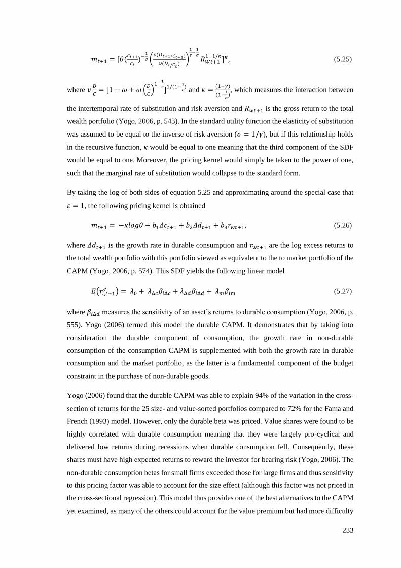
233

𝑚𝑡+1 = [𝜃(𝑐𝑡+1

𝑐𝑡)−

1

𝜎 (𝑣(𝐷𝑡+1/𝐶𝑡+1)

𝑣(𝐷𝑡/𝐶𝑡)

)

1

𝜀−

1

𝜎𝑅𝑊𝑡+1

1−1/𝜅]𝜅, (5.25)

where 𝑣𝐷

𝐶= [1 − 𝜔 + 𝜔 (

𝐷

𝐶)

1−1

𝜀]1/(1−

1

𝜀) and 𝜅 =

(1−𝛾)

(1−1

𝜎), which measures the interaction between

the intertemporal rate of substitution and risk aversion and 𝑅𝑤𝑡+1 is the gross return to the total

wealth portfolio (Yogo, 2006, p. 543). In the standard utility function the elasticity of substitution

was assumed to be equal to the inverse of risk aversion (𝜎 = 1/𝛾), but if this relationship holds

in the recursive function, 𝜅 would be equal to one meaning that the third component of the SDF

would be equal to one. Moreover, the pricing kernel would simply be taken to the power of one,

such that the marginal rate of substitution would collapse to the standard form.

By taking the log of both sides of equation 5.25 and approximating around the special case that

휀 = 1, the following pricing kernel is obtained

𝑚𝑡+1 = −𝜅𝑙𝑜𝑔𝜃 + 𝑏1𝛥𝑐𝑡+1 + 𝑏2𝛥𝑑𝑡+1 + 𝑏3𝑟𝑤𝑡+1, (5.26)

where 𝛥𝑑𝑡+1 is the growth rate in durable consumption and 𝑟𝑤𝑡+1 are the log excess returns to

the total wealth portfolio with this portfolio viewed as equivalent to the to market portfolio of the

CAPM (Yogo, 2006, p. 574). This SDF yields the following linear model

𝐸(𝑟𝑖,𝑡+1𝑒 ) = 𝜆0 + 𝜆Δ𝑐𝛽𝑖Δ𝑐 + 𝜆Δ𝑑𝛽𝑖Δ𝑑 + 𝜆𝑚𝛽𝑖m (5.27)

where 𝛽𝑖Δ𝑑 measures the sensitivity of an asset’s returns to durable consumption (Yogo, 2006, p.

555). Yogo (2006) termed this model the durable CAPM. It demonstrates that by taking into

consideration the durable component of consumption, the growth rate in non-durable

consumption of the consumption CAPM is supplemented with both the growth rate in durable

consumption and the market portfolio, as the latter is a fundamental component of the budget

constraint in the purchase of non-durable goods.

Yogo (2006) found that the durable CAPM was able to explain 94% of the variation in the cross-

section of returns for the 25 size- and value-sorted portfolios compared to 72% for the Fama and

French (1993) model. However, only the durable beta was priced. Value shares were found to be

highly correlated with durable consumption meaning that they were largely pro-cyclical and

delivered low returns during recessions when durable consumption fell. Consequently, these

shares must have high expected returns to reward the investor for bearing risk (Yogo, 2006). The

non-durable consumption betas for small firms exceeded those for large firms and thus sensitivity

to this pricing factor was able to account for the size effect (although this factor was not priced in

the cross-sectional regression). This model thus provides one of the best alternatives to the CAPM

yet examined, as many of the others could account for the value premium but had more difficulty

234

in explaining the size premium. The success of the durable CAPM was further enunciated by

Yogo (2006) as he showed that his model was the only one that passed the J-test of over-

identifying restrictions, achieved a higher ��2 than the Fama and French (1993) three-factor model

and yielded an insignificant intercept in the cross-sectional regression when compared to the

models of Lettau and Ludvigson (2001b), Piazzesi et al. (2003), Lustig and van Nieuwerburgh

(2005) and Parker and Julliard (2005).

Márquez and Nieto (2011) conducted an analysis of the durable CAPM for the U.S and Spanish

markets. For the U.S, some contrasting results to Yogo’s (2006) were obtained, as Márquez and

Nieto (2011) found that the model had little or no explanatory power irrespective of whether

consumption risk was modelled over a one quarter or three-year horizon (as per Parker & Julliard,

2005 discussed in chapter 3), with none of the three factors significant. One possible difference

for these results lies in the different test portfolios as Márquez and Nieto (2011) used size- and

industry-sorted portfolios compared to the size and value portfolios of Yogo (2006). These

contrasting results may therefore suggest that while the model has some ability to explain the

value (and to a lesser extent the size) anomaly, it could not explain all patterns in share returns.

When the model was tested in the form proposed by Yogo (2006) on the Spanish market, Márquez

and Nieto (2011) found that the model was able to explain a substantial portion of the cross-

sectional variation in size-sorted portfolios (53%), but yielded a negative risk premium on the

non-durable beta, which is inconsistent with economic intuition that shares with greater

correlation to non-durable consumption should earn higher returns. However, when consumption

risk was measured over a three-year horizon, both the durable and non-durable consumption betas

were priced with positive coefficients (the market portfolio was insignificant), with the model

able to explain 52% of the cross-sectional variation in the size portfolios. Despite this, the model

was still unable to fully account for the greater returns associated with the portfolio of small firms.

5.3 ANALYSIS


As indicated previously, finding a model that performs well empirically and also sheds light on

the factors which determine share returns is of critical importance. Macroeconomic variables are

seen as candidate determinants of share returns as they affect investor behaviour in their demand

for securities. In the previous chapter the role of labour income in the pricing of securities was

explored, while in this chapter, the relationship between housing wealth (and labour income) and

share prices is examined. A review of the theory and empirical evidence revealed that housing

wealth is inextricably linked to the stock market through consumption. Several asset pricing

235

models have been developed to account for this dynamic in the pricing of securities on the premise

that the consumption CAPM does not fully incorporate the risk arising from residential property.

These models had success in explaining the size and value anomalies. However, the models of

Piazzesi et al. (2003) and Lustig and van Nieuwerburgh (2005) have principally been tested in the

U.S with limited out-of-sample evidence, especially in emerging markets. To this author’s

knowledge, no one has sought to test these models that incorporate the risks arising from housing

wealth on the JSE. As outlined in section 5.1, the research objective of this chapter therefore is to

assess whether asset pricing models that include housing wealth can explain the cross-section of

South African share returns.

The real estate augmented CAPM of Kullmann (2003) and Funke et al (2010) is tested as this

provides initial information about the importance of real estate wealth in asset pricing. Labour

income is also included as a pricing factor in this model to consider the dual influence of these

two potentially important factors. Although these specifications do not tie consumption, labour

income, housing wealth and share returns together directly, the fact that their inclusion with the

market portfolio provides a more comprehensive measure of the total wealth portfolio, the

primary determinant of consumption, means that it does provide an indirect test of the

consumption theory. Thereafter, the conditioning variables of Piazzesi et al. (2003) and Lustig

and van Nieuwerburgh (2005) 𝛼 and 𝑚�� respectively, are computed and tested for their ability to

predict returns. The models which are derived from these composite variables, the CH-CAPM

and collateral CAPM based on Piazzesi et al. (2003) and Lustig and van Nieuwerburgh (2005)

respectively are then evaluated to assess their ability to explain returns. The composite variable

of Sousa (2010), 𝑐𝑑𝑎𝑦, was not examined as a result of the international findings that it provided

little or no additional explanatory power compared to 𝑐𝑎𝑦, while its ability to explain the cross-

sectional variation in share returns has yet to be tested. Finally, the model of Yogo (2006), which

uses the more generic measure of durable goods, is analysed. The details associated with the

computation of the pricing factors for each of these models are detailed in the following sections.

5.3.2 Computation of the Pricing Factors

5.3.2.1 The Real Estate CAPM

To measure the returns to real estate, it was necessary to distinguish commercial and residential

property as the two components reflect different fundamentals and are influenced by varying

economic forces. As highlighted in section 5.2.1, residential property is an investment, but also

generates a service flow and as such, the total return to home ownership should include price

appreciation and the value of the consumption services (Kullmann, 2003). Using an aggregate

house price index captures the former but is not able to quantify the service flow from housing

and this is exacerbated by the location specificity of real estate which creates additional

236

idiosyncratic risk for each individual which is impossible to capture. To employ an aggregate

price index thus necessitates the assumption that the implicit consumption benefit of housing is a

constant proportion of the return to home ownership (Fama & Schwert, 1977; Stambaugh, 1982).

Kullmann (2003) assessed the suitability of this assumption and found that the variance and

covariance (with the market) of the house price series principally materialised from the capital

gain component and not from the service flow. The use of an aggregate price index is therefore a

suitable proxy for returns to residential real estate and was thus utilised in this study to measure

the returns to residential property.

For this purpose, the ABSA house price index was used as it covered the entire sample period

whereas the indices published by other banks (such as First National Bank and Standard Bank)

have not been in existence for the entire period of the study. Moreover, given that these indices

rely on information determined from mortgage loan applications which were made and approved

by the individual banks (i.e. in-house data), the fact that ABSA has historically had the biggest

share of the domestic mortgage bond market (Luüs, 2003; Kloppers, 2008) means that it is likely

to provide more accurate information.68 The ABSA index based on the middle-class segment, for

all sized houses, both new and old (including improvements), was selected as this series is the

one predominantly reviewed by analysts in the market (Kloppers, 2008). The prices in this series

are already smoothed in order to limit the distortion caused by seasonality and outliers in the data.

The quarterly data was converted from nominal to real using CPI.

Although including commercial real estate in the model provides a broader measure of real estate

than the explicit focus on housing wealth in this study, it follows the method of Kullmann (2003)

and Funke et al. (2010) and thus allows for greater comparability in the results. Moreover, it also

provides some indication as to whether the effects of real estate wealth may be more closely

aligned to consumption (as is assumed to be the case in this study) or corporate risk. To measure

commercial real estate in the U.S, the index of REITs has been used (although REITs may also

include some investment in residential real estate, they are principally invested in commercial real

estate). REITs were only introduced in South Africa in May 2013 (Boshoff & Bredell, 2013) (post

the study period). However, as indicated in section 2.4.3.2, PUTs and PLSs have been listed on

the JSE for many years. According to Ernest and Young’s global REIT review, South African

PUTs have been considered equivalent to REITs (Lamprecht, 2013), whereas PLSs have a quite

68 To test the robustness of the results using the ABSA house price index, an attempt was made to obtain

data on the index maintained by Rode Property (which has been in existence for the entire sample period).

This index makes use of records of sales registered at the deeds office and thus, despite the time lag

involved, provides a more general overview of the market. However, this information was not obtainable.

237

different structure (Boshoff & Bredell, 2013).69 Accordingly, the FTSE/JSE PUT index (J255)

was used as the measure of commercial property in this study (this index was known as the IX48

under the previous JSE Actuaries Series). As mentioned in section 2.4.3.2, PUTs and PLSs were

excluded from the shares included in the portfolios and thus there was no risk of biasing the results

because of interaction between the test assets and pricing factors.

As mentioned, the real estate CAPM was also estimated with labour income as an additional factor

to examine the joint impact of these two measures of wealth. For this purpose, the

contemporaneous growth rate in labour income was used as it was found to perform slightly better

than the lagged growth rate in the analysis in the previous chapter.

5.3.2.2 CH-CAPM

The models proposed by Piazzesi et al. (2003) comprise two pricing factors – the growth in non-

housing consumption and α. Piazzesi et al. (2007) measured the former by subtracting housing

services from the conventional measure of aggregate consumption on non-durable goods and

services. The measure of housing services from the U.S Bureau of Economic Analysis (BEA) in

includes the cost of rental for both tenants and owners. The latter is imputed by assuming that the

owner rents the property to themselves based on rents charged for similar tenant-occupied housing

(Meyerhauser & Reinsdorf, 2007). Similar calculations are performed by the SARB for the

computation of total consumption expenditure in South Africa and this is reflected in the rent

series (KBP6069J) (SARB, 2013, pp. S112). This series, however, was only available annually.

A quarterly rental series was interpolated by using a cubic spline, as explained in chapter 3 and

then subtracted from the non-durable goods and services series to obtain non-housing

consumption.70 𝛼 was computed as the natural log of expenditure on non-housing consumption

divided by total consumption on non-durable goods and services.

5.3.2.3 𝑚��

In order to estimate the collateral CAPM, it was necessary to compute 𝑚𝑦, with this ratio

comprising two components - labour income and housing value. For the former, the series used

in the previous models was employed. To measure housing value, Lustig and van Nieuwerburgh

69 The FTSE/JSE introduced a REIT index which was backdated but only to 2009 and therefore was of

limited use for this study given the 1990 to 2013 sample period. They used the PUTs as the components

thereof which thus validates the use of the PUT index in this study. 70 A second housing services series was computed by assuming that rent was a constant percentage of total

consumption on non-durable goods and services throughout the year. The correlation between the two

quarterly measures of housing services was high (0.98). The series from the cubic spline was favoured,

however, because using that based on the assumption of rent being a constant proportion of consumption

per annum would yield values for the expenditure share that were constant throughout the year.

238

(2005) used three different series - the value of outstanding home mortgages, the market value of

residential real estate wealth and the current cost of the net stock of owner- and tenant-occupied

residential fixed assets. The SARB monthly series of the value of home mortgages outstanding

(KBP1480M) was used to measure housing value, as it was considered an equivalent measure to

Lustig and van Nieuwerburgh’s (2005) first series, with the observation at the end of each quarter

used. To ensure that the results from this analysis were not sensitive to the measure of housing

wealth, an alternative proxy was sought. The SARB provides a series documenting annual

household wealth in residential buildings (KBP6921J).71 To obtain quarterly observations, the

wealth in residential building was assumed to be a constant proportion of total wealth per annum

and then applied to the quarterly wealth figures used in chapter 4.72

As explained in section 5.2.3.2, 𝑚𝑦 is measured in a similar manner to 𝑐𝑎𝑦 and thus, the Johansen

(1988) and Stock and Watson (1993) methods used to estimate 𝑐𝑎𝑦 (as explained in chapter 4)

were also used to compute this ratio, with both an intercept and trend included in the cointegrating

relation. However, for 𝑚𝑦, the approach of Johansen (1988) is particularly useful, as it allows the

restriction that the coefficient on labour income is equal to minus one (𝜛 = −1) to be imposed.

To assess the appropriateness of this restriction, Lustig and van Nieuwerburgh (2005) compared

the correlation of the estimates of 𝑚𝑦 based on the restricted and unrestricted models. However,

in the Johansen (1988) approach it is possible to test whether the restriction holds using a chi-

squared test of binding restrictions, and thus this test was implemented. If the restriction was

found to be supported by the data, then the values of 𝑚𝑦 from the restricted regression were used.

Finally, to ensure that 𝑚𝑦 was positive, the method followed by Lustig and van Nieuwerburgh

(2005), outlined in equation 5.16, of rescaling the ratio to yield the collateral scarcity ratio 𝑚��

was followed (𝑚��𝑡 = 𝑚𝑦𝑡𝑚𝑎𝑥 − 𝑚𝑦𝑡).

5.3.2.4 The Durable CAPM

The new pricing factor introduced in the model of Yogo (2006) is the growth rate in durable

consumption. Durable goods have a longer life than one quarter and therefore the growth rate in

the stock of durable goods rather than the growth rate in expenditure on durable goods needs to

be computed. To this end, Yogo (2006) obtained annual data from the BEA that captured the net

stock of consumer durable goods. Using this information, and a quarterly depreciation rate of

71 This series was computed by Aron and Muellbauer (2006); the details of which are provided in their

study. Although they did create a quarterly series thereof, this was not available from the SARB. Several

efforts to obtain this directly from Dr. Aron were unsuccessful. 72 This was considered to be more accurate than using a cubic spline especially considering that this series

was used as an input into cointegration tests, as more information was obtainable about movements between

quarters given the ratio and quarterly wealth than the cubic spline provides.

239

6%73, Yogo (2006) constructed a series for the stock of durable goods accounting for expenditure

each quarter, as per equation 5.22 (𝐷𝑡 = (1 − 𝛿)𝐷𝑡−1 + 𝐸𝑡). Márquez and Nieto (2011), in testing

Yogo’s (2006) model, were unable to access similar information on the stock of durable goods

for Spain, with only quarterly expenditure information available. Consequently, they used

historical data from prior to the commencement of their study period to devise an estimate of the

total stock of durable goods at the beginning of the sample period. For depreciation, Márquez and

Nieto (2011) used a rate of 4.7% per quarter, a rate applicable only for motor vehicles, on the

basis that the largest proportion of durable consumption expenditure in Spain was on vehicles.

The SARB does not avail information on the net stock of durable goods for the country. However,

as a memo item to the balance sheet of households, they do provide an annual measure of the net

wealth of households including durable consumer goods (KBP6933J). An approximation of the

durable consumer goods portion was thus calculated by subtracting the net wealth of households

from this series to use as the starting point in equation 5.22. This was combined with the quarterly

expenditure on durable goods (KBP6050K)74. No information was available from the SARB

about the depreciation rate; however, using the annual information, it was ascertained that an

average depreciation rate of 6% per quarter is used. The fact that this depreciation rate is

equivalent to that used in the US is not surprising as the lifespan of a good should not be country

dependent; provided that quality is similar. Accordingly, this rate was applied to obtain the

quarterly durable stock series as per equation 5.22.

This computation of durable stock may be limited because it does not include semi-durable goods

and the starting point was implied from the data and not computed directly. Therefore, a broader

series of durable consumption was computed, principally following the methodology of Márquez

and Nieto (2011). Data was obtained for the expenditure on durable goods for 48 quarters75 prior

to the starting date of the regressions so as to be able to compute an appropriate value for the stock

of durable goods at the start of quarter three of 1990. The largest component of semi-durable

73 The depreciation rate of 6% per quarter equates to approximately 22% per annum. This value represents

the average of the depreciation rates associated with all durable goods. For example, tyres and other car

accessories have a depreciation rate of 62% per year while at the other end, household furniture has a

depreciation rate of only 12% per annum. Given the aggregate estimates of durable consumption, it is not

possible to ascertain what portion is comprised of each of these components to apply the individual

depreciation rates; thus justifying Yogo’s (2006) application of the average. Bernanke (1985) and Baxter

(1996) also use this average annual rate of 22% in their analyses. 74 For the quarterly expenditure series on durable (and semi-durable) goods, the series not adjusted for

seasonality were utilised as the actual amount of the expenditure per quarter was needed which is not

captured when the smoothing process is applied, as this reflects an annualised expenditure estimate. 75 48 quarters were used as with a depreciation rate of 6% after twelve years the good would be worth only

approximately 5% of its original value due to depreciation and therefore would have little impact on the

value of the stock of durable goods.

240

expenditure (KBP6055K) by South Africans is on clothing and footwear, followed by motorcar

tyres, parts and accessories, and household textiles (SARB, 2013, pp. S112). The BEA depreciates

tyres and accessories in the U.S by 15.5% per quarter implying that after approximately two to

three years, the goods will have little value. This rate was considered appropriate for the semi-

durable series in this study. Accordingly, for this series, information for the 20 quarters76 prior to

the commencement of the study period was obtained to be able to compute the stock of semi-

durable goods as at quarter three 1990. With this information and the quarterly expenditure on

both series, the stocks of durable and semi-durable goods were computed as per equation 5.22

and then added together to provide a comprehensive measure of the total stock of durable goods.

5.3.3 Methodology

To test the asset pricing models described above, the approaches outlined in the preceding

chapters were used, with the principle attention on the cross-sectional regression results, with

GMM used as a test of robustness thereof. As outlined in chapter 3, the estimates of the cross-

sectional risk premia from the time-series data and the tests of the significance of the pricing

errors from the time-series regressions on each portfolio are only appropriate for tests of static

models with traded factors. In this chapter, the majority of models did not satisfy these criteria

such that the time-series tests were only conducted for the real estate CAPM and the real estate

CAPM with labour income.

As is evident, most of the models examined that incorporate the effects of real estate into the

pricing equation, either directly or indirectly, are built from the foundation of the consumption

CAPM. To ensure that the results of these models were not sensitive to the measurement period

of consumption, as investors may not react immediately to changes in consumption (Parker &

Julliard, 2005), the non-contemporaneous measure over a three-quarter horizon was also tested.

Márquez and Nieto (2011) also used non-contemporaneous measures in their tests of the durable

CAPM, and in fact, they tested the model with the long-run growth rates in both durable and non-

durable consumption, which was also implemented in this study. Where the models examined

utilised conditioning variables, these were lagged appropriately by an additional two periods.

5.4 RESULTS

In this section the results from the various models tested are presented. Firstly, the real estate

CAPM is examined so as to assess the direct role real estate wealth has on pricing size- and value-

sorted portfolios and industry-sorted portfolios. Secondly, the results from the forecasting

76 After 20 quarters the good will only be worth approximately 4% of its original value.

241

analysis of Piazzesi et al.’s (2007) conditioning variable, 𝛼, are presented, with the results from

the asset pricing models built around this factor examined thereafter. Following this, the findings

from the tests of Lustig and van Nieuwerburgh’s (2005) 𝑚�� factor are presented and finally, the

tests of the durable CAPM are presented and discussed.

5.4.1 The Real Estate CAPM and Real Estate CAPM with Labour Income


As with the multi-factor models examined in chapters 3 and 4, prior to estimating any regressions,

the correlations between the pricing factors were examined to ascertain whether any of the factors

moved closely together. Highly correlated pricing factors would bias the coefficient estimates

obtained in the time-series regressions, which are then used as inputs into the cross-sectional

regressions leading to potentially incorrect inferences being made. Only limited co-movement

between the two components of real estate (0.38) was observed, as shown in Table 5-1, suggesting

that commercial and residential real estate are driven by different factors.

Table 5-1: Correlation Matrix of the Pricing Factors in the Real Estate CAPM and Real Estate

CAPM with Labour Income

𝑟𝑚𝑒 𝑟𝐶𝑅𝐸

𝑒 𝑟𝑅𝑅𝐸𝑒 ∆𝑦

𝑟𝑚𝑒 1

𝑟𝐶𝑅𝐸𝑒 0.35 1

𝑟𝑅𝑅𝐸𝑒 0.19 0.38 1

∆𝑦 0.17 0.47 0.48 1

This table shows the correlation coefficients between the excess market returns (𝑟𝑚𝑒 ), commercial (𝑟𝐶𝑅𝐸

𝑒 )

and residential real estate returns (𝑟𝑅𝑅𝐸𝑒 ) and the growth rate in labour income (∆𝑦) for the period June 1990

to April 2013.

Commercial real estate moved more closely with the market than residential real estate. It has

been noted in the literature that the returns on REITs often exhibit the properties of the market

returns rather than the direct real estate returns (Westerheid, 2006) which appears to be true for

South Africa. Kullmann (2003) also noted very little co-movement (correlation of 0.12) between

the returns to the U.S market index and residential real estate over the period of her study. The

relatively high co-movement between both commercial and real estate returns and labour income

of 0.47 and 0.48 respectively was a surprising finding, as it suggests that these two important

components of the total wealth portfolio are closely related. However, these correlation measures

were still less than 0.5 (the cut-off identified in chapter 3) and therefore it was not considered

necessary to orthogonalise any of the pricing factors in these real estate models.

The risk premium estimates from the two models are shown in Table 5-2. The average excess

returns from residential real estate (𝑟𝑅𝑅𝐸𝑒 ) were positive over the period 1990 to 2013, consistent

with the housing price boom in South Africa during the period reviewed. The risk premium was

242

found to be weakly significant at 10% compared to the insignificant market risk premium. In

contrast to the good performance of residential real estate over the period, the returns to

commercial real (𝑟𝐶𝑅𝐸𝑒 ) estate were negative. This poor performance confirms that the drivers of

residential and commercial real estate differ in that a substantial portion of the returns to

commercial real estate arise from rental income as opposed to capital appreciation as is the case

with residential real estate. However, although negative, the risk premium estimate was

insignificant. If the theory is appropriate, then the risk premia should be positive and significant

suggesting that higher risk, as captured by a greater sensitivity to the factors, should be rewarded

with higher returns. Based on the sample averages, only residential real estate and labour income

(as noted in chapter 4) satisfy this requirement. However, as indicated previously, these risk

premia do not take into consideration other important information from the test portfolios and do

not account for possible pricing errors and as such the risk premia estimates from the cross-

sectional regressions are usually favoured. These are examined in the following section.

Table 5-2: Time-Series Estimates of the Factor Risk Premia for the Real Estate CAPM and Real

Estate CAPM with Labour Income

𝜆𝑚 𝜆𝐶𝑅𝐸 𝜆𝑅𝑅𝐸 𝜆Δ𝑦

𝜆𝑓

t-statistic

0.85

(0.83)

-0.36

(0.40)

0.78*

(1.68)

0.60**

(2.50)

In this table the factor risk premia (𝜆𝑓) for the market (𝜆𝑚), commercial (𝜆𝐶𝑅𝐸) and residential real estate

(𝜆𝑅𝑅𝐸) and labour income (𝜆Δ𝑦) are shown. These are estimated as the time-series average, 𝐸𝑡(𝑓), for the

period June 1990 to April 2013. Beneath each coefficient the t-statistic computed using the Newey and

West (1987) standard errors is shown in round parentheses. *, ** and *** indicate significance at 10%, 5%

and 1% respectively for the t-tests.

Other useful information about the role of real estate in pricing securities can, however, still be

obtained from the time-series analysis, with the focus in this regard on the regressions on each of

the test portfolios. The summary results thereof are shown in Table 5-3, with the full information

for the 16 size and value and industry portfolio shown in Tables D-1 and D-2 in the appendix (p.

333 and p. 334 respectively). In the CAPM and CAPM with labour income, the majority of the

intercepts were significant, with the same also true for the models augmented with real estate.

This conclusion was confirmed by the GRS test of the joint pricing errors. Moreover, as shown

in Tables D-1 and D-2, these significant pricing errors were associated with the portfolios

comprising small and value shares suggesting that the anomalies remain even after adjusting for

risk associated with residential and commercial real estate. Funke et al. (2010) also found that the

majority of the intercepts for the 25 size- and value-sorted portfolios were significant when

evaluating the real estate augmented CAPM (with only commercial real estate) in the U.S.

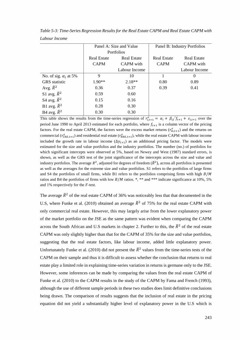
243

Table 5-3: Time-Series Regression Results for the Real Estate CAPM and Real Estate CAPM with

Labour Income

Panel A: Size and Value

Portfolios

Panel B: Industry Portfolios

Real Estate

CAPM

Real Estate

CAPM with

Labour Income

Real Estate

CAPM

Real Estate

CAPM with

Labour Income

No. of sig. 𝛼𝑖 at 5% 9 10 1 0

GRS statistic 1.90** 2.18** 0.80 0.89

Avg. ��2 0.36 0.37 0.39 0.41

S1 avg. ��2 0.59 0.60

S4 avg. ��2 0.15 0.16

B1 avg. ��2 0.28 0.30

B4 avg. ��2 0.30 0.30

This table shows the results from the time-series regression of 𝑟𝑖,𝑡+1𝑒 = 𝛼𝑖 + 𝛽𝑖𝑓′𝑓𝑡+1 + 휀𝑖,𝑡+1 over the

period June 1990 to April 2013 estimated for each portfolio, where 𝑓𝑡+1 is a column vector of the pricing

factors. For the real estate CAPM, the factors were the excess market returns (𝑟𝑚,𝑡+1𝑒 ) and the returns on

commercial (𝑟𝐶𝑅𝐸,𝑡+1𝑒 ) and residential real estate (𝑟𝑅𝑅𝐸,𝑡+1

𝑒 ), while the real estate CAPM with labour income

included the growth rate in labour income (∆𝑦𝑡+1) as an additional pricing factor. The models were

estimated for the size and value portfolios and the industry portfolios. The number (no.) of portfolios for

which significant intercepts were observed at 5%, based on Newey and West (1987) standard errors, is

shown, as well as the GRS test of the joint significance of the intercepts across the size and value and

industry portfolios. The average 𝑅2, adjusted for degrees of freedom (��2), across all portfolios is presented

as well as the averages for the extreme size and value portfolios. S1 refers to the portfolios of large firms

and S4 the portfolios of small firms, while B1 refers to the portfolios comprising firms with high 𝐵/𝑀

ratios and B4 the portfolios of firms with low 𝐵/𝑀 ratios. *, ** and *** indicate significance at 10%, 5%

and 1% respectively for the F-test.

The average ��2 of the real estate CAPM of 36% was noticeably less that that documented in the

U.S, where Funke et al. (2010) obtained an average ��2 of 75% for the real estate CAPM with

only commercial real estate. However, this may largely arise from the lower explanatory power

of the market portfolio on the JSE as the same pattern was evident when comparing the CAPM

across the South African and U.S markets in chapter 2. Further to this, the ��2 of the real estate

CAPM was only slightly higher than that for the CAPM of 35% for the size and value portfolios,

suggesting that the real estate factors, like labour income, added little explanatory power.

Unfortunately Funke et al. (2010) did not present the ��2 values from the time-series tests of the

CAPM on their sample and thus it is difficult to assess whether the conclusion that returns to real

estate play a limited role in explaining time-series variation in returns is germane only to the JSE.

However, some inferences can be made by comparing the values from the real estate CAPM of

Funke et al. (2010) to the CAPM results in the study of the CAPM by Fama and French (1993),

although the use of different sample periods in these two studies does limit definitive conclusions

being drawn. The comparison of results suggests that the inclusion of real estate in the pricing

equation did not yield a substantially higher level of explanatory power in the U.S which is

244

consistent with the results on the JSE. Moreover, the real estate augmented CAPM also failed to

match the 54% explanatory power of the Fama and French (1993) three-factor model on the JSE,

as observed in chapter 3.

As with the size- and value-sorted portfolios, the results for the industry portfolios confirmed that

the market portfolio was the principle factor in capturing time-series variation in returns as the

inclusion of residential and commercial real estate into the pricing equations yielded little change

in the explanatory power. Although the pricing errors were insignificant, this pattern has arisen

with these portfolios under all models evaluated in this study, which is attributable to the lack of

variation in portfolio returns as opposed to a good fitting specification.


The cross-sectional results for the real estate models are shown in Table 5-4. The measures of the

explanatory power indicate that the inclusion of real estate yielded a substantial increase in ��2

from 27% for the CAPM to 56% for the size and value portfolios, although this is still lower than

the Fama and French (1993) model on the JSE of 70%. Funke et al. (2010) found that the real

estate CAPM (albeit only with commercial real estate) was able to explain a greater portion (77%)

of the variation across equivalent portfolios in the U.S. Although the R2 of 48% obtained by

Kullmann (2003) for the U.S., using both residential and commercial real estate, was closer to

that obtained for the South African market, the use of different portfolios as the test assets makes

direct comparisons difficult.

The market and commercial real estate risk premia entered with the wrong signs in the real estate

augmented CAPM, but they were insignificant. The residential real estate risk premium, in

contrast, was positive and significant. This finding is consistent with the estimate of the time-

series risk premium, as shown in Table 5-2, however, the cross-sectional estimate did not satisfy

the test proposed by Lewellen et al. (2010) that it should be equal to the time-series average. The

finding of the significant role of residential real estate in the pricing of the cross-section of returns

on the JSE is similar to Kullmann’s (2003) findings for the size and beta-sorted portfolios on the

U.S and the conclusion drawn by Cochrane (1996) that residential real estate is more important

to investors than commercial real estate. However, these finding are different to those of

Kullmann (2003) and Funke et al. (2010) with respect to the size- and value-sorted portfolios,

where they both found commercial real estate returns to be priced. The commercial property

sector in South Africa has historically been quite small – in fact in 2000, this sector was worth

only R5 billion compared to the R270 billion in May 2013 (Lamprecht, 2013b, para. 5). Despite

this growth, it still comprises only 3.5% of the total market capitalisation of the JSE with

companies such as SABMiller 3.3 times larger than this sector (Lloyd, 2013, para. 4).

245

Table 5-4: Cross-Sectional Regression Results for the Real Estate CAPM and Real Estate CAPM with Labour Income


Real Estate CAPM Real Estate CAPM

with Labour Income

Real Estate CAPM with

SMB and HML

Real Estate CAPM Real Estate CAPM

with Labour Income

𝜆0 3.99

(2.25)**

{1.51}

3.97

(2.23)**

{1.28}

4.24

(2.27)**

{1.86}*

3.24

(3.57)***

{3.28}***

3.13

(3.24)***

{2.96}***

𝜆𝑚 -2.55

(-1.12)

{-0.75}

-3.32

(-1.45)

{-0.83}

-3.65

(-1.52)

{-1.24}

-2.41

(-1.39)

{-0.64}

-2.32

(-1.38)

{-0.62}

𝜆𝐶𝑅𝐸 -0.26

(-0.12)

{-0.08}

-1.31

(-0.61)

{-0.35}

-1.26

(-0.58)

{-0.48}

0.03

(0.03)

{0.01}

0.34

(0.17)

{0.10}

𝜆𝑅𝑅𝐸 2.55

(3.23)***

{2.17}**

2.22

(2.80)***

{1.60}

1.93

1.90*

{1.73}*

0.79

(1.10)

{0.67}

0.82

(1.26)

{0.73}

𝜆∆𝑦 -1.13

(-1.51)

{-0.98}

0.05

(0.10)

{0.06}

𝜆∆𝑐

𝜆𝑆𝑀𝐵 2.62

(3.76)***

{3.01}***

𝜆𝐻𝑀𝐿 2.45

(2.86)***

{2.29}**

𝑅2

(��2)

0.65

(0.56)

0.71

(0.60)

0.77

(0.66)

0.72

(0.55)

0.73

(0.46)

246



obtained from the time-series regressions. For the real estate CAPM, the factor loadings included the sensitivity to the excess market returns (𝛽𝑖𝑚) and the returns on commercial

(𝛽𝑖𝑐𝑟𝑒) and residential real estate (𝛽𝑖𝑟𝑟𝑒), while the real estate CAPM with labour income also included a factor loading on the growth rate in labour income (𝛽𝑖∆𝑦). Finally, for

the real estate CAPM with size and value, the sensitivity to the two Fama and French (1993) factors - the returns on a zero-cost portfolio long small firm shares and short big

firm shares (𝛽𝑖𝑆𝑀𝐵) and a zero-cost portfolio long firms with high 𝐵/𝑀 ratios and short firms with low 𝐵/𝑀 ratios (𝛽𝑖𝐻𝑀𝐿) – were also included. Beneath each coefficient in

round parentheses is the t-statistic computed using the Fama and MacBeth (1973) standard errors, while the second t-statistic in curly parentheses was calculated using the

Shanken (1992) standard errors. The Wald statistic provides a test of the joint significance of the coefficients and the Q-statistic tests the joint significance of the model pricing

errors. The values of both of these statistics computed using Shanken’s (1992) standard errors are shown in curly parentheses. RMSE refers to the root mean squared pricing

error across the portfolios. The 𝑅2 is Jagannathan and Wang’s (1996) cross-sectional measure of explanatory power and ��2 is adjusted for the number of pricing factors. The

AIC refers to the Akaike information criteria and was computed similarly to Jagannathan and Wang’s (1996) 𝑅2. *, ** and *** indicate significance at the 10%, 5% and 1%

levels respectively for the various tests.

AIC 0.82 0.79 0.53 -0.92 -1.26


{5.26}*

13.19***

{4.33}

25.81***

{16.66)**

3.14

{0.86}

3.52

{0.92}

RMSE 0.97 1.08 0.86 0.37 0.37


{65.51}***

31.01***

{94.31}***

14.73

{41.16}**

(3.73)

{4.43}

(3.91)

{4.67}

247

Accordingly, the results obtained may reflect the relative insignificance of this sector in the risk-

return relationship (especially when compared to the U.S), or the fact that the impact of real estate

on share returns is more closely correlated with the consumption channel than the lending or

collateral channels of companies.

A plot of the residential real estate betas from the real estate CAPM in Figure 5-1 shows that these

betas are higher for the portfolios comprising small firms compared to those comprising large

firms. This graph also reveals some evidence that the value portfolios had greater risk, although

the difference between the risk measures for high and low value shares was less monotonic than

amongst the size quartiles. Funke et al. (2010) found that the commercial real estate betas were

positively related to the 𝐵/𝑀 ratio, and while the opposite was true across the size quintiles, the

relationship was less definitive. Thus, their results seemed to suggest a stronger link between the

𝐵/𝑀 ratio and commercial real estate factor whereas there appears to be a stronger link between

size and the residential real estate measure in this South African sample. The negative betas for

some of the large and growth portfolios suggests that these shares do not offer investors a risk

premium (and in effect penalise investors in terms of returns earned) as they effectively hedge

against adverse movements in property prices. This indicates that individuals prefer to avoid

holding shares that are highly correlated with their residential properties.

Figure 5-1: Residential Real Estate Betas from the Real Estate CAPM for the Size and Value

Portfolios

This figure plots the residential real estate betas (𝛽𝑖𝑅𝑅𝐸) estimated from the time-series regression of 𝑟𝑖,𝑡+1𝑒 =

𝛼𝑖 + 𝛽𝑖𝑚𝑟𝑚,𝑡+1𝑒 + 𝛽𝑖𝐶𝑅𝐸𝑟𝐶𝑅𝐸,𝑡+1

𝑒 + 𝛽𝑖𝑅𝑅𝐸𝑟𝑅𝑅𝐸,𝑡+1𝑒 + 휀𝑖,𝑡+1 over the period June 1990 to April 2013 for each

of the 16 size and value portfolios, where 𝑟𝑚,𝑡+1𝑒 are the excess market returns and 𝑟𝐶𝑅𝐸,𝑡+1

𝑒 and 𝑟𝑅𝑅𝐸,𝑡+1𝑒 are

the excess returns on commercial and residential real estate. S1 refers to the portfolios of large firms and

S4 the portfolios of small firms while B1 refers to the portfolios of firms with high 𝐵/𝑀 ratios and B4 the


248

The inclusion of labour income resulted in only a small rise in explanatory power and, consistent

with the evidence obtained in the tests of the CAPM with labour income, this factor entered with

an a-theoretical sign, although it was not significant. Thus, there was no evidence to suggest that

these two factors jointly determined returns, with real estate subsuming the effects of labour

income in the U.S (Kullmann, 2003), while in South Africa no role was found for labour income.

As can be seen in the final row of Table 5-3, the null hypothesis that the pricing errors were equal

to zero was rejected for both models despite the evidence that the inclusion of the residential beta

appeared to be able to account for some of the higher returns associated with small and value

firms. However, the same was also found to be true for the three-factor model of Fama and French

(1993) in chapter 3. The evidence in Figure 5-2, which shows the pricing errors from the real

estate CAPM, confirms that the inclusion of the real estate factors helped to explain the size

anomaly but had less success with the value phenomenon as the portfolios which lie furthest away

from the 45-degree line are principally those with high and low 𝐵/𝑀 ratios.

Figure 5-2: Pricing Errors from the Real Estate CAPM for the Size and Value Portfolios


𝑒 = 𝜆0 + 𝜆𝑚𝛽𝑖𝑚 + 𝜆𝐶𝑅𝐸𝛽𝑖𝐶𝑅𝐸 +

𝜆𝑅𝑅𝐸𝛽𝑖𝑅𝑅𝐸 + 𝜂𝑖 over the period June 1990 to April 2013 across the 16 size and value portfolios, where 𝛽𝑖𝑚,

𝛽𝑖𝑐𝑟𝑒 and 𝛽𝑖𝑟𝑟𝑒 measure the sensitivity of the portfolio returns to the excess market returns and the returns

on commercial and residential real estate respectively. S1 refers to the portfolios of large firms and S4 the

portfolios of small firms while B1 refers to the portfolios of firms with high 𝐵/𝑀 ratios and B4 the


The inclusion of the two real estate factors in the pricing equations yielded no significant

coefficients in the tests on the industry portfolios, as is evident in Table 5-4. In addition, none of

the other slope coefficients were priced. In light of this, it is of limited value evaluating the

explanatory power of the models and the size of the pricing errors because they are likely to only

249

reflect the limited variation across the industry portfolios as opposed to the ability of the models

to explain patterns in returns.

Given that the real estate CAPM performed reasonably well in the tests conducted on the size and

value portfolios, an additional test of the model was conducted by adding the SMB and HML

factors to the pricing equation to assess whether they remained priced in the presence of real

estate. The results from this model are also shown in Table 5-4. An ��2 of 66% was obtained

which exceeded that of the real estate CAPM indicating that size and value still contain substantial

information that is not captured in the real estate factors. The residential beta remained significant,

although the risk premium was smaller. Similarly to the additional test of the (C)CAPM with 𝑐𝑎𝑦

in chapter 4, SMB and HML were both found to be priced suggesting that residential real estate

cannot capture the size and value anomalies. This differs from the finding of Funke et al. (2010)

for the U.S who found that they were insignificant in the real estate augmented CAPM. However,

the results do suggest that part of the anomalous returns on the JSE can be attributed to the

sensitivity of small and value shares to residential real estate.


The results from the GMM regressions, displayed in Table 5-5, were identical to those obtained

in the cross-sectional regressions. That is, the most striking finding was the significance of the

residential real estate returns in the SDF and the significant risk premium on residential real estate

in the beta-return equations for the size and value portfolios across both specifications. As is

evident in panel B of the table, the signs were also consistent with the view that the portfolios that

were more highly correlated with residential real estate yielded higher returns. None of the other

coefficients were found to be important in pricing securities or were priced in the cross-section.

Thus, even the inclusion of residential real estate as a pricing factor could not salvage the market

risk-return relationship and in addition, the pricing errors for each model were still found to differ

significantly from zero, as captured by the J-statistics. Despite the clear role for residential real

estate in the pricing of the size and value portfolios, the same was not found to be true for the

industry portfolios.

The results from the real estate models thus reveal that residential real estate does play a role in

explaining differences in returns across the size and value portfolios and thus potentially shows a

link between the returns from housing wealth and consumption, given that total wealth is the key

driver of consumption patterns. The fact that commercial real estate was found to be insignificant

may suggest that the risk of real estate in the company’s assets is not a key determinant of

investment returns but, given the very small size of this sector on the JSE such conclusions may

be inappropriate. Further consideration of the link between real estate and corporate risk is

250

presented in chapter 6. The analysis of other models which account for the impact of housing

wealth on consumption are reviewed in the following sections.

Table 5-5: GMM Regression Results for the Real Estate CAPM and Real Estate CAPM with

Labour Income


Real Estate

CAPM

Real Estate CAPM

with Labour

Income

Real Estate

CAPM

Real Estate

CAPM with

Labour Income

𝑏𝑚 -0.00

(-0.27)

-0.00

(-0.18)

0.01

(-0.95)

0.01

(0.79)

𝑏𝐶𝑅𝐸 0.04

(-1.35)

0.05

(-1.49)

0.03

(-0.78)

0.03

(0.79)

𝑏𝑅𝑅𝐸 -0.40***

(-5.43)

-0.38***

(-3.72)

-0.20

(-1.54)

-0.21

(-1.47)

𝑏∆𝑦 -0.13

(-0.44)

-0.05

(-0.23)

𝑏∆𝑐

J-statistic 32.40*** 21.84** 5.32 4.732

𝜆𝑚 0.40

(0.27)

0.30

(0.18)

-1.21

(-0.97)

-1.07

(-0.80)

𝜆𝐶𝑅𝐸 -2.47

(-1.37)

-2.37

(-1.22)

-1.70

(-0.79)

-1.96

(-0.80)

𝜆𝑅𝑅𝐸 2.75***

(5.52)

2.60***

(3.76)

1.35

(1.56)

1.46

(1.49)

𝜆∆𝑦 0.37

(0.45)

0.14

(0.22)

𝜆∆𝑐

This table shows the coefficients from Hansen’s (1982) optimal two-stage GMM estimation over the period

June 1990 to April 2013 of the SDF 𝑚𝑡+1 = 𝛼 + 𝑏′𝑓𝑡+1, where 𝑚𝑡+1 is the SDF, 𝑓𝑡+1 is a column vector

of the pricing factors and 𝛼 was normalised to one. For the real estate CAPM 𝑓𝑡+1 included the excess

market returns (𝑟𝑚,𝑡+1𝑒 ) and the returns on commercial (𝑟𝐶𝑅𝐸,𝑡+1

𝑒 ) and residential real estate (𝑟𝑅𝑅𝐸,𝑡+1𝑒 ), while

the real estate CAPM with labour income also included the growth rate in labour income (∆𝑦𝑡+1). The

models were estimated for the size and value portfolios and the industry portfolios. The transformed risk

premia (𝜆) are presented in the bottom half of the table and were computed from the SDF coefficients as

𝜆 = −𝑣𝑎𝑟(𝑓)𝑏, where 𝑣𝑎𝑟(𝑓) is the variance of the pricing factor. Beneath both the 𝑏’s and 𝜆’s the t-

statistics are displayed in round parentheses, with the standard errors of the transformed 𝜆’s computed using

the delta method. *, ** and *** indicate significance at the 10%, 5% and 1% levels respectively for the

various tests.

5.4.2 The CH-CAPM

5.4.2.1 Descriptive Statistics and the Predictive Power of 𝛼

The properties of Piazzesi et al.’s (2007) 𝛼 for South Africa are displayed in Table 5-6. On average

87% (𝑒−0.14) of total consumption of households was on non-housing services, which is slightly

higher than that observed in the U.S of approximately 82% by Piazzasi et al. (2007) and

251

Table 5-6: Summary Statistics of α

𝛼


Avg. -0.14

Std Dev. 0.02

𝜌(1) 0.94

ADF statistic -1.56

KPSS statistic 0.14


𝑟𝑚𝑒 -0.18

𝑟𝑒𝑙𝑎𝑡𝑖𝑣𝑒 0.03


𝐷/𝑃 -0.08

𝐸/𝑃 -0.09

𝑐𝑎𝑦 0.07

𝑠𝑦 0.55

In panel A of this table the descriptive statistics of the expenditure share on non-housing consumption

relative to total consumption, 𝛼, over the period July 1990 to April 2013 are shown. These include the

average (avg.), standard deviation (std. dev.), first-order autocorrelation (𝜌(1)), ADF and KPSS test

statistics (using a trend and intercept). For the ADF test, the critical values from MacKinnon (1996) were

used while for the KPSS test, the Kwiatkowski et al. (1992) critical values were used. In panel B, the

correlation coefficients between 𝛼 and the traditional forecasting variables – the term spread (𝑠𝑝𝑟𝑒𝑎𝑑),

relative T-bill (𝑟𝑒𝑙𝑎𝑡𝑖𝑣𝑒), 𝐷/𝑃, 𝐸/𝑃 and the lagged excess market returns (𝑟𝑚𝑒 ) are presented, as well the

correlation with the measures introduced in chapter 4 - 𝑐𝑎𝑦 and 𝑠𝑦. *, ** and *** indicate significance at

the 10%, 5% and 1% levels respectively for the ADF and KPSS tests.

Rasmussen (2006). Although these U.S studies covered much longer periods, the fact that a

smaller portion of South African household’s expenditure is utilised for housing services than in

the U.S may reflect lower rental (both imputed and actual) costs. This may be attributable to both

lower standards of living in South African as well as the greater reliance on government provided

housing which lowers the average rental costs. The ADF test demonstrates that this series is non-

stationary, with the KPSS test presenting a contrasting conclusion that the series is stationary.

Given the previous discussions regarding the advantage of the KPSS test when the series has a

root close to the unit boundary (as the autocorrelation measure confirms is the case for 𝛼), the

conclusion from the KPSS test that the ratio was stationary was relied upon. Moreover, similarly

to 𝑠𝑦, this conclusion is consistent with intuition that neither expenditure on non-housing services

nor total consumption can grow to dominate the other.

Unlike the measures derived from labour income analysed in chapter 4, 𝛼 does not have

particularly strong relationships with the traditional forecasting variables, with the highest

correlation of 0.21 being with the term spread. A negative relationship with the excess real market

returns was evident, which supports the theoretical paradigm of Piazzesi et al. (2007), as it implies

that shares have low payoffs in severe recessions when housing consumption is relatively low

252

(and 𝛼 is high). The high correlation between 𝛼 and 𝑠𝑦 arises due to the reliance of both measures

on total consumption expenditure.

The non-logged expenditure share is depicted in Figure 5-3. During the first half of the period,

the expenditure share was reasonably constant although it did increase from 1990 through to 1994.

This relatively smooth pattern however contrasts with the substantial movements in the series

observed in the second half of the period, where for example, the expenditure share declined from

approximately 88% in 2002 to less than 85% in 2005. The fall in the expenditure share during the

financial crisis of 2008 and 2009 is opposite to what is predicted by Piazzesi et al.’s (2007) model

that the expenditure share should be high during a recession as the consumption of non-housing

services relative to total consumption is high.

Figure 5-3: The Value of α in South Africa

This figure shows the share of total consumption spent on non-housing consumption goods and services,

denoted 𝛼, in South Africa over the period June 1990 to April 2013.

The regression coefficients and ��2 values from the forecasting regressions using 𝛼 are displayed

in Table 5-7. 𝛼 had no ability to predict share returns at longer horizons, but there was weak

evidence (at 10%) of predictive power for returns on the JSE for one- and two-quarters ahead.

However, the explanatory power of 2% and 4% respectively for these two horizons was also much

lower than the equivalent values when 𝑐𝑎𝑦 was used as the forecasting variable of 8% and 7%

respectively. A higher value of 𝛼 should predict higher returns as a higher expenditure share of

non-housing consumption is associated with recessions; however, a negative coefficient was

obtained in these regressions. This result, while inconsistent with Piazzesi et al.’s (2007) results

for the U.S, matches what was observed in the graphical evidence.

253

Table 5-7: Forecasts of Multiple Quarter Excess Real Market Returns using α

𝑧𝑡

Forecast horizon (H) in quarters

1 2 4 6 8 12

𝛼 -1.69*

(-1.88)

[0.02]

{0.02}

-3.01*

(-1.69)

[0.04]

{0.03}

-5.35

(-1.58)

[0.07]

{0.05}

-7.24

(-1.57)

[0.09]

{0.04}

-8.45

(-1.57)

[0.09]

{0.04}

-9.24

(-1.48)

[0.07]

{0.00}

𝐷/𝑃



𝛼

1.48

(1.21)

0.94

(0.76)

3.73***

(2.88)

-2.58**

(-2.59)

[0.17]

{0.08}

3.72

(1.60)

1.85

(0.78)

5.60***

(2.71)

-4.51***

(-2.66)

[0.19]

{0.07}

7.21***

(3.09)

9.70***

(3.54)

3.78

(1.44)

-8.10***

(-3.14)

[0.32]

{0.07}

11.85***

(4.61)

3.70

(1.63)

13.61***

(3.59)

-11.32***

(-3.36)

[0.44]

{0.06}

13.83***

(3.89)

-0.92

(-0.31)

11.45***

(3.22)

-12.16***

(-3.00)

[0.47]

{0.05}

20.24***

(4.08)

4.90

(1.50)

-2.31

(-0.68)

-10.76**

(-2.48)

[0.56]

{0.04}


over the period June 1990 to April 2013, where 𝑧𝑡 is the column vector of predictor variables and H is the

forecast horizon. For the first regression 𝑧𝑡 included the expenditure share on non-housing consumption as

a proportion of total consumption (𝛼), while for the second regression this was combined with the term

spread (𝑠𝑝𝑟𝑒𝑎𝑑), relative T-bill (𝑟𝑒𝑙𝑎𝑡𝑖𝑣𝑒) and 𝐷/𝑃. Beneath each coefficient in round parentheses is the

t-statistic computed using the Newey and West (1987) standard errors. The regression 𝑅2, adjusted for

degrees of freedom, ��2, is shown in square parentheses, with Hodrick’s (1992) ��2 presented thereunder in

curly parentheses. *, ** and *** indicate significance at 10%, 5% and 1% respectively for the t-tests.

When combined with 𝐷/𝑃, the term spread and relative T-Bill yield, 𝛼 was significant at every

horizon; however, in all circumstances the coefficient was negative. The fact that 𝛼 was found to

be significant in the joint regressions, at horizons greater than two quarters ahead, which was not

the case when the variable was analysed individually, suggests either that the forecasting equation

is not well-specified or that the explanatory variables are highly correlated. The latter was not

found to be true in Table 5-6 and thus points to important missing variables from the forecasting

equation. After adjusting for the persistent nature of the 𝐷/𝑃 ratio (using Hodrick’s, 1992 ��2),

the differences in explanatory power between the identical regression without 𝛼 in Table 3-3 were

small suggesting that the contribution of 𝛼 was relatively minor.

As highlighted in section 5.2.3.1, although there was some mixed evidence internationally

regarding the predictability of 𝛼, with some studies showing short-run and others long-run

forecasting power, all studies found that this ratio contained useful information about future

business cycles at some frequency and the coefficients were positive. Thus, the South African

market appears to be notably different from the U.S and U.K where these studies were performed,

as 𝛼 predicted a negative relationship with future returns. The negative sign reflects that levels of

non-housing consumption declined further than consumption on housing services during

254

recessions. Such a pattern is not inconceivable in the emerging South African market where the

relatively low income levels of the country mean that housing services are not accessible to the

majority (which these aggregate figures reflect). Consumption on housing services is thus already

low, and in many instances, housing services are provided by government, such that during

recessions, consumers drop off non-housing consumption more than housing services. Further

examination of this ratio is thus warranted to ascertain whether this observation is unique to South

Africa or whether the same applies in other emerging markets.


The one-quarter growth rate in non-housing consumption (shown in Table 5-8) was identical to

the growth rate in consumption on non-durable goods and services over the period 1990 to 2013,

but did exhibit slightly more volatility (standard deviation of 1.67% compared to 1.53%). The

latter trend suggests that consumption on housing services is less volatile than consumption on

non-housing services and non-durable goods, which is similar to Piazzesi et al.’s (2007) finding

for the U.S. The growth rate computed over three-quarters exhibited almost identical properties

to the growth rate on consumption of non-durable goods and services, as shown in Table 3-11.

The correlations between the pricing factors in the various collateral housing models were found

to be reasonably small in magnitude, as shown in Table D-3 in the appendix (p. 335) and thus it

was not necessary to orthogonalise any of these explanatory variables before estimating the

regressions. The cross-sectional results from the collateral models are displayed in Table 5-9. For

the size- and value-sorted portfolios, the consumption CAPM with non-housing consumption

performed as poorly as when total consumption on non-durable goods and services was used

(examined in chapter 3), as the negative R2 shows. However, whereas the total consumption

growth rate was a priced factor, the same was not true for the non-housing consumption growth

rate. Accordingly, the pricing errors of this model were large, as reflected both by the RMSE of

1.83 and the significant chi-squared statistic. Lustig and van Nieuwerburgh (2005) also found this

consumption growth rate to be insignificant and although Piazzesi et al. (2003) documented the

opposite, this may be attributable to the differing sample periods used across these two U.S

studies. Measuring consumption growth over a three quarter horizon, in the spirit of Parker and

Julliard’s (2005) recommendations, did not salvage the model, as the consumption risk premium

remained insignificant, as shown in Table D-4 in the appendix (p. 336).

Turning to the three models proposed by Piazzesi et al. (2003), the results indicate that the

conditional CH-CAPM and the (C)CAPM were able to explain 48% and 45% of the cross-

sectional variation in the size and value portfolios respectively, with the AIC suggesting that the

latter was marginally superior. The two non-contemporaneous conditional models also performed

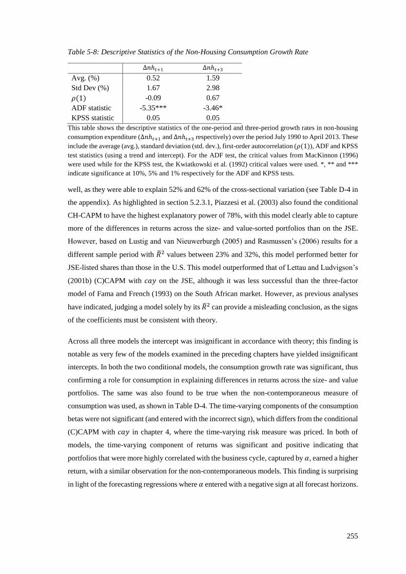
255

Table 5-8: Descriptive Statistics of the Non-Housing Consumption Growth Rate

∆𝑛ℎ𝑡+1 ∆𝑛ℎ𝑡+3

Avg. (%) 0.52 1.59

Std Dev (%) 1.67 2.98

𝜌(1) -0.09 0.67

ADF statistic -5.35*** -3.46*

KPSS statistic 0.05 0.05

This table shows the descriptive statistics of the one-period and three-period growth rates in non-housing

consumption expenditure (∆𝑛ℎ𝑡+1 and ∆𝑛ℎ𝑡+3 respectively) over the period July 1990 to April 2013. These

include the average (avg.), standard deviation (std. dev.), first-order autocorrelation (𝜌(1)), ADF and KPSS

test statistics (using a trend and intercept). For the ADF test, the critical values from MacKinnon (1996)

were used while for the KPSS test, the Kwiatkowski et al. (1992) critical values were used. *, ** and ***

indicate significance at 10%, 5% and 1% respectively for the ADF and KPSS tests.

well, as they were able to explain 52% and 62% of the cross-sectional variation (see Table D-4 in

the appendix). As highlighted in section 5.2.3.1, Piazzesi et al. (2003) also found the conditional

CH-CAPM to have the highest explanatory power of 78%, with this model clearly able to capture

more of the differences in returns across the size- and value-sorted portfolios than on the JSE.

However, based on Lustig and van Nieuwerburgh (2005) and Rasmussen’s (2006) results for a

different sample period with ��2 values between 23% and 32%, this model performed better for

JSE-listed shares than those in the U.S. This model outperformed that of Lettau and Ludvigson’s

(2001b) (C)CAPM with 𝑐𝑎𝑦 on the JSE, although it was less successful than the three-factor

model of Fama and French (1993) on the South African market. However, as previous analyses

have indicated, judging a model solely by its ��2 can provide a misleading conclusion, as the signs

of the coefficients must be consistent with theory.

Across all three models the intercept was insignificant in accordance with theory; this finding is

notable as very few of the models examined in the preceding chapters have yielded insignificant

intercepts. In both the two conditional models, the consumption growth rate was significant, thus

confirming a role for consumption in explaining differences in returns across the size- and value

portfolios. The same was also found to be true when the non-contemporaneous measure of

consumption was used, as shown in Table D-4. The time-varying components of the consumption

betas were not significant (and entered with the incorrect sign), which differs from the conditional

(C)CAPM with 𝑐𝑎𝑦 in chapter 4, where the time-varying risk measure was priced. In both of

models, the time-varying component of returns was significant and positive indicating that

portfolios that were more highly correlated with the business cycle, captured by 𝛼, earned a higher

return, with a similar observation for the non-contemporaneous models. This finding is surprising

in light of the forecasting regressions where 𝛼 entered with a negative sign at all forecast horizons.

256

Table 5-9: Cross-Sectional Regression Results for the Collateral Housing Models


Consumption

CAPM with

non-housing

consumption

CH-CAPM (C)CAPM

with non-

housing

consumption

Conditional

CH-CAPM

(C)CAPM with

non-housing

consumption with

size and value

Consumption

CAPM with

non-housing

consumption

CH-CAPM (C)CAPM

with non-

housing

consumption

Conditional

CH-CAPM

𝜆0 3.08

(3.16)**

{3.14}**

1.06

(1.05)

{0.62}

1.62

(1.51)

{0.81}

1.12

(1.03)

{0.66}

2.21

(1.95)*

{1.50}

1.64

(4.47)**

{4.47}**

1.42

(3.96)**

{1.90}*

1.56

(1.77)*

{1.77}*

2.37

(2.08)**

{1.64}

𝜆Δ𝑛ℎ 0.19

(0.88)

{0.40}

-0.72

(-1.26)

{-0.68}

1.56

(3.00)**

{1.68}*

1.14

(1.72)*

{0.97}

0.69

(1.13)

{0.86}

-0.08

(-0.27)

{-0.12}

-0.74

(-1.60)

{-0.66}

-0.01

(-0.04)

{-0.02}

-1.00

(-1.56)

{-1.01}

𝜆Δ𝛼

-0.40

(-1.05)

{-0.78}

0.04

(0.21)

{0.13}

-0.21

(-1.49)

{-0.78}

-0.17

(-1.45)

{-1.00}

𝜆𝛼 0.99

(2.20)**

{1.18}

0.84

(1.89)*

{1.20}

0.71

(1.68)*

{1.24}

-0.13

(-0.12)

{-0.10}

0.40

(0.40)

{0.29}

𝜆Δnh𝛼 -1.18

(-0.99)

{-0.53}

-0.43

(-0.33)

{-0.21}

-0.21

(-0.17)

{-0.13}

-0.14

(-0.10)

{-0.08}

0.53

(0.45)

{0.30}

𝜆Δ𝛼𝛼 0.02

(0.14)

{0.09}

-0.04

(-0.15)

{-0.16}

𝜆SMB 2.49

(3.56)***

{2.69}***

𝜆HML 2.36

257

(2.72)***

{2.06}**

𝑅2

(��2)

0.00

(-0.07)

0.45

0.36

0.56

(0.45)

0.65

(0.48)

0.82

(0.73)

0.57

(0.51)

0.86

(0.82)

0.55

(0.27)

0.95

(0.49)

AIC 1.52 1.06 0.95 0.98 0.31 -0.96 -1.86 -0.65 -2.47

Wald

statistic

0.77

{0.16}

10.89

{3.62}

14.82**

{4.27}

6.07

{2.45}

24.00***

{13.77}**

0.07

{0.02}

6.16

{1.21}

0.03

{0.02}

4.93

{2.22}

RMSE 1.83 1.36 1.09 1.21 0.78 0.71 0.29 0.65 0.14

Q-statistic 210.12**

{212.86}**

29.75**

{84.79}**

44.79**

{110.62}**

54.87**

{189.92}**

13.85*

{45.68}***

4.86

{5.91}

1.12

{4.88}

4.10

{4.13}

0.28

{0.45}



obtained from the time-series regressions. For the non-housing consumption CAPM, the factor loading was the sensitivity to the growth rate in non-housing consumption

(𝛽𝑖∆𝑛ℎ), while for the CH-CAPM, the factor loadings included 𝛽𝑖∆𝑛ℎ and the sensitivity to changes in the expenditure share of non-housing consumption to total consumption

(𝛽𝑖∆𝛼). For the (C)CAPM, the factor loadings were 𝛽𝑖∆𝑛ℎ, the sensitivity to the conditioning variable, 𝛽𝑖𝛼 and the sensitivity to the scaled non-housing consumption growth rate

(𝛽𝑖∆𝑛ℎ𝛼), while for the conditional CH-CAPM, the factor loadings included 𝛽𝑖∆𝑛ℎ, 𝛽𝑖𝛼 , 𝛽𝑖∆𝛼, 𝛽𝑖∆𝑛ℎ𝛼 and the sensitivity to the scaled change in the expenditure share (𝛽𝑝∆𝛼𝛼).

Finally, for the (C)CAPM with size and value, the sensitivity to the two Fama and French (1993) factors - the returns on a zero-cost portfolio long small firm shares and short

big firm shares (𝛽𝑖𝑆𝑀𝐵) and a zero-cost portfolio long firms with high 𝐵/𝑀 ratios and short firms with low 𝐵/𝑀 ratios (𝛽𝑖𝐻𝑀𝐿) – were also included. Beneath each coefficient

in round parentheses is the t-statistic computed using the Fama and MacBeth (1973) standard errors, while the second t-statistic in curly parentheses was calculated using the

Shanken (1992) standard errors. The Wald statistic provides a test of the joint significance of the coefficients and the Q-statistic tests the joint significance of the model pricing

errors. The values of both of these statistics computed using Shanken’s (1992) standard errors are shown in curly parentheses. RMSE refers to the root mean squared pricing

error across the portfolios. The 𝑅2 is Jagannathan and Wang’s (1996) cross-sectional measure of explanatory power and ��2 is adjusted for the number of pricing factors. The

AIC refers to the Akaike information criteria and was computed similarly to Jagannathan and Wang’s (1996) 𝑅2. *, ** and *** indicate significance at 10%, 5% and 1%


258

To make sense of this apparent contradiction, an analysis of the expenditure share betas was

conducted, with the results shown in Figure 5-4. As can be seen, the portfolios comprising ‘very

small’ and small firms had positive expenditure share betas while the majority of the betas for the

other quartiles were negative. Thus, these results suggest that the high returns associated with the

small and ‘very small’ shares on the JSE may be a consequence of their sensitivity to the

composition risk of consumption, whereas larger shares effectively act as a hedge against this

risk. There was also some evidence that those portfolios comprising shares with high 𝐵/𝑀 ratios

had higher betas than those portfolios of low 𝐵/𝑀 ratios, but this pattern was less monotonic than

across the size quintiles.

Figure 5-4: Conditional Betas using α for the Size and Value Portfolios

This figure plots the expenditure share betas (𝛽𝑖𝛼) estimated from the time-series regression of 𝑟𝑖,𝑡+1𝑒 =

𝛼𝑖 + 𝛽𝑖∆𝑛ℎ𝛥𝑛ℎ𝑡+1 + 𝛽𝑖𝛼𝛼𝑡 + 𝛽𝑖∆𝑛ℎ𝛼Δnh𝑡+1𝛼𝑡 + 휀𝑖,𝑡+1 over the period June 1990 to April 2013 for each

of the 16 size and value portfolios, where 𝛥𝑛ℎ𝑡+1 is the growth rate in non-housing consumption

expenditure, 𝛼𝑡 is the expenditure share on non-housing consumption relative to total consumption and

Δnh𝑡+1𝛼𝑡 is the scaled growth rate in consumption expenditure. S1 refers to the portfolios of large firms

and S4 the portfolios of small firms while B1 refers to the portfolios of firms with high 𝐵/𝑀 ratios and B4

the portfolios of firms with low 𝐵/𝑀 ratios.

This pattern can also be reconciled with the results from the predictive regressions. As mentioned

in chapter 3, the excess market returns which were used as the dependent variable in the

forecasting regression are generated from the ALSI, an index which is heavily-weighted towards

the large shares, with the largest five shares accounting for approximately 42% of the total market

value as at February 2009, for example. Accordingly, if the excess market returns effectively

represent the movement of large shares and large shares act as a hedge against composition risk

compared to very small shares which pay out when 𝛼 is high, then this may explain the negative

coefficients observed in the forecasting regressions.

259

The differenced 𝛼 added little explanatory power in the two collateral models, as in both cases

the coefficient on this parameter was insignificant. In fact, as the Wald tests indicate, only the

(C)CAPM yielded jointly significant coefficients. Accordingly, the analysis of the coefficients

supports Piazzesi et al.’s (2003) conditional CH-CAPM on the JSE. Further analysis of the pricing

errors of this model, as shown in Figure 5-5, confirmed that it was able to account for some of the

size anomaly but was not able to explain the differences in returns to value and growth shares,

with substantial pricing errors still associated with the extreme portfolios. Consistent with the

other models examined in the preceding chapters, the pricing errors remained significant,

although the RMSE of 1.09 was lower than many of the other models.

Figure 5-5: Pricing Errors from the Conditional CH-CAPM for the Size and Value Portfolios

This figure plots the pricing errors from the cross-sectional regression ��𝑖,𝑡+1𝑒 = 𝜆0 + 𝜆Δ𝑛ℎ𝛽𝑖∆𝑛ℎ + 𝜆α𝛽𝑖𝛼 +

𝜆Δ𝛼𝛽𝑖∆𝛼 + 𝜆Δ𝑛ℎ𝛼𝛽𝑖∆𝑛ℎ𝛼 + 𝜆Δ𝛼𝛼𝛽𝑖∆𝛼𝛼 + 𝜂𝑖 over the period June 1990 to April 2013 across the 16 size and

value portfolios, where 𝛽𝑖∆𝑛ℎ, 𝛽𝑖𝛼 , 𝛽𝑖∆𝛼, 𝛽𝑖∆𝑛ℎ𝛼 and 𝛽𝑖∆𝛼𝛼 measure the sensitivity of the portfolio returns to

the growth rate in non-housing consumption, the expenditure share on non-housing consumption relative

to total consumption, the change in the expenditure share, and the scaled growth rate in non-housing

consumption and change in expenditure share respectively. S1 refers to the portfolios of large firms and S4



As with the real estate CAPM in the preceding section, an additional test of the suitability of these

collateral housing models was conducted by including the SMB and HML factors into the pricing

equation to ascertain whether they are still priced in the presence of the other explanatory

variables. For this purpose, the (C)CAPM with non-housing consumption was used rather than

the conditional CH-CAPM as the additional parameters in the latter model were not found to add

substantial value given that they were insignificant. The results from this model are also presented

in Table 5-9 and showed that both the Fama and French (1993) two factors remained significant

and effectively crowded out the effects of the other pricing factors suggesting that the static and

S1B1

S1B2

S1B3

S1B4

S2B1S2B2S2B3S2B4

S3B1

S3B2

S3B3

S3B4

S4B1

S4B2S4B3

S4B4

0

7

0

1

2

3

4

5

6

7

0 1 2 3 4 5 6 7

Fit

ted

Ret

urn

s

Realised Returns

260

conditional non-housing consumption betas and the sensitivity of the portfolio returns to future

business cycles as predicted by the expenditure ratio were not sufficient to explain the two well-

known anomalies. However, the risk premium on the 𝛼 beta retained its significance

demonstrating that some of the information contained in this ratio that explains returns is not

captured by the ad hoc size and value measures.

For the industry portfolios, the results in Table 5-9 mirror those obtained for all previous

specifications as the slope coefficients were all insignificant. This demonstrates that neither

growth in the consumption of non-housing services nor 𝛼 could explain patterns across these

portfolios, even after accounting for time-variation in risk and return.


To ensure the robustness of the results of the tests of these collateral models based on the cross-

sectional approach, the discount factors for these models were also estimated using GMM, with

the results thereof and the transformed risk premia presented in Table 5-10. For the industry

portfolios, one of the pricing factors in the CH-CAPM was significant in the SDF, with the

transformed risk premium also indicating that the factor was priced. Accordingly, portfolios

which were more highly correlated with changes in the composition risk of consumption earned

a higher return; consistent with intuition. Interestingly, however, this factor was not found to be

important in explaining differences in returns across the size- and value-sorted portfolios, but, at

the very least, indicates that some pricing factors can still account for differences in returns across

the industry portfolios despite their relatively low cross-sectional variation which makes them

difficult to price.

The growth rate in non-housing consumption was an important variable in helping to explain

differences in returns across the size- and value-sorted portfolios for all three models of Piazzesi

et al. (2003), which is similar to the results observed in the cross-sectional regressions. Again, in

the two CH-CAPM specifications, the sensitivity to composition risk was not found to be priced.

Turning to the conditional models, the time-varying intercept was significant in the SDF and the

transformed risk premia were positive and significant, similarly to the cross-sectional results. The

only notable difference was the fact that the time-varying non-housing consumption beta was

significant in the SDF and priced in the return-beta framework, however, it entered with the wrong

sign. Despite the relatively good performance of some of these collateral models in identifying

significant pricing factors, the J-statistics still indicated that the null hypothesis that the pricing

errors were equal to zero was rejected.

261

Table 5-10: GMM Regression Results for the Collateral Housing Models


Consumption CAPM

with non-housing

consumption

CH-CAPM (C)CAPM with

non-housing

consumption

Conditional

CH-CAPM

Consumption CAPM

with non-housing

consumption


non-housing

consumption

Conditional

CH-CAPM

𝑏Δ𝑛ℎ -0.61

(-1.48)

-0.45***

(-3.22)

-0.59***

(-5.86)

-0.53***

(-3.85)

-0.25

(1.30)

0.21

(1.10)

0.01

(0.05)

0.17

(0.69)

𝑏Δ𝛼 -6.27

(-1.03)

3.55

(1.13)

-3.76**

(-2.36)

2.65

(1.31)

𝑏𝛼 -0.55***

(-5.02)

-0.39***

(-2.89)

0.51

(1.24)

0.22

(0.49)

𝑏Δ𝑛ℎ𝛼 0.47

(1.01)

0.43**

(2.24)

0.01

(0.06)

0.11

(0.34)

𝑏Δ𝛼𝛼 -0.89

(-1.03)

-0.46

(-0.24)

J-statistic 31.72*** 33.59*** 39.01*** 33.82*** 5.05 4.69 2.57 1.07

𝜆Δ𝑛ℎ 1.69

(1.06)

1.26***

(3.25)

1.63***

(5.91)

1.46***

(3.87)

0.71

(1.32)

-0.59

(1.00)

-0.03

(0.04)

-0.47

(-0.69)

𝜆Δ𝛼 0.40

(1.05)

-0.23

(-0.68)

0.24**

(2.38)

-0.17

(0.14)

𝜆𝛼 1.45***

(5.07)

1.03*

(1.67)

-1.36

(-1.26)

1.20

(0.45)

𝜆Δ𝑛ℎ𝛼 -4.13

(1.06)

-3.74***

(-3.62)

-0.10

(-0.05)

0.92

(7.24)

𝜆Δ𝛼𝛼 0.15

(0.52)

0.08

(1.95)

This table shows the coefficients from Hansen’s (1982) optimal two-stage GMM estimation over the period June 1990 to April 2013 of the SDF 𝑚𝑡+1 = 𝛼 + 𝑏′𝑓𝑡+1, where

𝑚𝑡+1 is the SDF, 𝑓𝑡+1 is a column vector of the pricing factors and 𝛼 was normalised to one. For the consumption CAPM with non-housing consumption, 𝑓𝑡+1 included the

262

growth rate in non-housing consumption (∆𝑛ℎ𝑡+1), while ∆𝑛ℎ𝑡+1 was also a factor in the CH-CAPM coupled with the change in the expenditure share of non-housing

consumption to total consumption (∆𝛼). For the (C)CAPM, the factors included ∆𝑛ℎ𝑡+1, the conditioning variable – 𝛼 – and the scaled non-housing consumption growth rate

∆𝑛ℎ𝑡+1𝛼, while for the conditional CH-CAPM, the pricing factors included ∆𝑛ℎ𝑡+1, 𝛼, ∆𝛼, ∆𝑛ℎ𝑡+1𝛼 and the scaled change in the expenditure share ((∆𝛼𝛼). The transformed

risk premia (𝜆) are presented in the bottom half of the table and were computed from the SDF coefficients as 𝜆 = −𝑣𝑎𝑟(𝑓)𝑏, where 𝑣𝑎𝑟(𝑓) is the variance of the pricing factor.

Beneath both the 𝑏’s and 𝜆’s the t-statistics are displayed in round parentheses, with the standard errors of the transformed 𝜆’s computed using the delta method. Hansen’s

(1982) J-statistic for the test of the pricing errors is also shown. *, ** and *** indicate significance at 10%, 5% and 1% respectively for the various tests.

263

The results from the collateral housing models thus provide some insights into the size and value

anomalies. In particular, these models point to the importance of time-varying returns when

business cycles are forecast with 𝛼, with small shares being more sensitive to this factor and hence

necessitating a higher risk premium to induce investors to hold these securities. However, the

model was not able to explain all of this anomaly and did not capture the variation across the

value and growth portfolios. Nevertheless, it did indicate that composition risk is an important

factor in measuring bad states of the economy.

5.4.3 The Collateral CAPM

5.4.3.1 Estimates of my

The ADF and KPSS tests conducted on the value of mortgages outstanding (𝑚𝑜𝑡) and household

wealth in residential buildings (𝑏𝑢𝑖𝑙𝑑𝑡), the two proxies used for housing wealth, confirm that the

series are integrated of order one, as shown in panel A of Table 5-11. Thus, these series were used

in cointegration tests with labour income, which was found to be integrated of the same order in

chapter 4. These cointegration test results are documented in panel B of Table 5-11. For the DLS

method using the value of outstanding mortgages, there was evidence of a long-run relationship

between housing wealth and labour income at 10%, and this conclusion was robust to the number

of lead and lag parameters used in the specification. Johansen’s (1988) approach yielded a similar

conclusion of the existence of a cointegrating relationship as the null hypothesis of no relationship

was rejected at 5% for both the trace and ME tests. When the housing value was measured based

on residential buildings, only the trace and ME tests showed evidence of a long-run relationship,

as the Phillips and Ouliaris (1990) test statistic was insignificant. Overall the finding of a

relationship between labour income and housing wealth was largely robust to the measurement

of the latter, which is consistent with the findings of Lustig and van Nieuwerburgh (2005) and

Rasmussen (2006) for the U.S. The results for the tests of the parameters and asset pricing models

were not found to differ substantially across these two measures and thus in the interest of brevity

only those based on the value of outstanding mortgages are presented as this definition most

closely resembles that employed in the seminal study.77

The restriction that the coefficient on labour income was equal to minus one was tested under

Johansen’s (1988) approach, with the insignificant chi-squared statistic (0.13) confirming that this

restriction was supported by the data. Accordingly, the estimate of 𝑚𝑦 from this particular

equation was used for the remainder of the analysis as it enabled the restriction to be imposed.

The cointegrating vector was thus given as follows

77 Unlike 𝑐𝑎𝑦, the error correction model was not examined as the estimates from the estimation of 𝑚𝑦 do

not directly tie in to share return predictability because asset wealth is not a component of the model.

264

𝑚𝑜𝑡 = 𝑦𝑡 + 0.01𝑡 + 2.73. (5.28)

Table 5-11: Estimates for the Components of my

Panel A: Unit Root and Stationarity Tests

In levels In first differences

ADF Statistic KPSS Statistic ADF Statistic KPSS Statistic

𝑚𝑜𝑡 -1.44 0.13* -3.43*** 0.17

𝑏𝑢𝑖𝑙𝑑𝑡 -2.06 0.18** -8.99*** 0.28

Panel B: Cointegration Tests

Method Statistic

Stock and Watson (1993) Phillips and Ouliaris (1990) 𝜏-statistic

𝑦𝑡 and 𝑚𝑜𝑡 -3.64*

𝑦𝑡 and 𝑏𝑢𝑖𝑙𝑑𝑡 -1.34

Johansen (1988)

(r = 0 only)

Trace statistic ME statistic

𝑦𝑡 and 𝑚𝑜𝑡 26.03** 20.41**

𝑦𝑡 and 𝑏𝑢𝑖𝑙𝑑𝑡 24.56** 14.42*

In panel A of the table, the ADF and KPSS tests of the two measures of housing wealth – mortgages

outstanding (𝑚𝑜𝑡) and residential buildings (𝑏𝑢𝑖𝑙𝑑𝑡) are shown for the variables in levels (with an intercept

and trend) and first differences (intercept only). For the ADF test, the critical values from MacKinnon

(1996) were used while for the KPSS test the Kwiatkowski et al. (1992) critical values were used. In panel

B, the results from two cointegration tests between the measures of housing wealth and labour income (𝑦𝑡)

(identified to be integrated of order one in tests conducted in chapter 4) are displayed. The first used the

single-equation DLS method of Stock and Watson (1993) where the Phillips and Ouliaris (1990) test

statistic was computed. The critical values were obtained from MacKinnon (1996). The second test was the

multi-equation method of Johansen (1988) where both the trace and maximum-eigenvalue (ME) statistics

were computed. The critical values were obtained from MacKinnon et al. (1999). *, ** and *** indicate

significance at 10%, 5% and 1% respectively for the various tests.

5.4.3.2 Descriptive Statistics and the Predictive Power of 𝑚��

Figure 5-6 depicts 𝑚𝑦 over the sample period. The ratio increased during the early years as well

as from the end of 2003 to mid-2009 with both of these timeframes coinciding with growth

periods in the South African economy. Accordingly, this graph indicates that a high value of this

ratio arose during good business periods. Moreover, the falls in 𝑚𝑦 from 1998 to 2000 and again

at the onset of the 2008/2009 financial crisis suggests that investors had less collateral during

these periods to protect their labour income; thus making investors more risk-averse. Therefore,

there does appear to be evidence to suggest that 𝑚𝑦 was correlated with business conditions.

The descriptive statistics of the collateral scarcity ratio (𝑚��) are shown in Table 5-12. The mean

of 0.32 was similar to the U.S series of 0.30 computed by Rasmussen (2006), although the South

African series exhibited less volatility and greater persistence than the U.S ratio. The South

265

Figure 5-6: The Value of 𝑚𝑦 for South Africa

This figure shows the housing collateral ratio, denoted 𝑚𝑦, in South Africa over the period June 1990 to

April 2013.

Table 5-12: Summary Statistics of 𝑚��

𝑚��


Avg. 0.32

Std. Dev. 0.15

𝜌(1) 0.92


𝑟𝑚𝑒 -0.02

𝑟𝑒𝑙𝑎𝑡𝑖𝑣𝑒 -0.30


𝐷/𝑃 -0.25

𝐸/𝑃 -0.23

𝑐𝑎𝑦 0.00

𝑠𝑦 -0.54

𝛼 0.75

In panel A of this table the descriptive statistics of the housing scarcity ratio, 𝑚��, over the period July 1990

to April 2013 are shown. These include the average (avg.), standard deviation (std. dev.) and first-order

autocorrelation (𝜌(1)). In panel B, the correlation coefficients between 𝑚�� and the traditional forecasting

variables – the term spread (𝑠𝑝𝑟𝑒𝑎𝑑), relative T-bill (𝑟𝑒𝑙𝑎𝑡𝑖𝑣𝑒), 𝐷/𝑃, 𝐸/𝑃 and the lagged excess market

returns (𝑟𝑚𝑒 ) are presented, as well the correlation with the measures introduced in chapters 4 and 5 – 𝑐𝑎𝑦,

𝑠𝑦 and 𝛼.

African series did exhibit higher autocorrelation but was stationary by construction as it is the

cointegrating residual. 𝑚�� moved quite closely with the term spread and relative T-Bill yield,

which is not surprising given that the value of housing wealth, as measured by the value of

mortgages outstanding, is likely to be correlated with the interest rate. 𝑚�� was even more strongly

correlated, in absolute terms, with 𝛼 and 𝑠𝑦, which confirms the important role of labour income

266

in these measures. The negative relationship with 𝑠𝑦 simply reflects their differing computations

which gives rise to movement in opposite directions during different stages of the business cycle

Although 𝑚�� and 𝛼 frame the impact of housing on the consumption decision of an investor

differently (composition risk versus hedging shocks to labour income) the two measures do move

closely together.

The results for the forecasting tests of 𝑚�� are shown in Table 5-13. The coefficients are positive

in accordance with the supposition that a low housing collateral ratio (a high value of 𝑚��) predicts

a high future risk premium. However, none of the coefficients were significant at any horizon and

this is confirmed by low and negative ��2 estimates. Moreover, despite the high persistence of this

ratio, it did not give rise to inflated explanatory power measures (as shown by Hodrick’s ��2)

confirming that this variable had little power to predict future period market returns. Moreover,

when combined with other forecasting variables, 𝑚�� remained insignificant and had little impact

on the significance of the other explanatory variables.

Table 5-13: Forecasts of Multiple Quarter Excess Real Market Returns using 𝑚��

Regressors Forecast horizon (H) in quarters

1 2 4 6 8 12

𝑚�� 0.14

(0.12)

[-0.01]

{0.00}

0.53

(0.24)

[-0.01]

{0.00}

1.24

(0.34)

[-0.01]

{0.00}

2.15

(0.50)

[-0.00]

{0.00}

3.03

(0.71)

[0.00]

{0.00}

4.65

(1.11)

[0.01]

{0.00}

𝐷/𝑃



𝑚��

1.61

(1.23)

0.49

(0.40)

3.79***

(2.71)

2.12

(1.68)

[0.14]

{0.06}

3.53

(1.30)

0.92

(0.40)

5.13**

(2.14)

2.70

(1.21)

[0.12]

{0.05}

6.53**

(2.17)

1.88

(0.67)

8.28**

(2.65)

4.03

(1.29)

[0.19]

{0.07}

10.84***

(2.80)

0.79

(0.29)

11.26***

(2.80)

5.42

(1.57)

[0.26]

{0.05}

12.31***

(2.68)

-4.35

(-1.40)

8.07**

(2.02)

4.76

(1.18)

[0.30]

{0.04}

18.47***

(3.22)

-5.42

(-1.31)

0.43

(0.10)

1.56

(033)

[0.45]

{0.03}



and 𝑧𝑡 is the column vector of predictor variables. For the first regression 𝑧𝑡 included the housing scarcity

ratio (𝑚��), while for the second regression this was combined with the term spread (𝑠𝑝𝑟𝑒𝑎𝑑), relative T-

bill (𝑟𝑒𝑙𝑎𝑡𝑖𝑣𝑒) and 𝐷/𝑃. Beneath each coefficient in round parentheses is the t-statistic computed using the

Newey and West (1987) adjusted standard errors. The regression 𝑅2, adjusted for degrees of freedom, ��2,

is shown in square parentheses, with Hodrick’s (1992) ��2 presented thereunder in curly parentheses. *, **

and *** indicate significance at 10%, 5% and 1% respectively for the t-tests.

The finding that 𝑚�� had no forecasting power at short-run horizons is consistent with the evidence

for the U.S market, as Lustig and van Nieuwerburgh (2005), Rasmussen (2006) and Sousa (2012)

267

all obtained positive but insignificant coefficients and ��2 estimates close to zero. Sousa’s (2012)

findings for the U.K market contradict this, as he found 𝑚�� to have significant forecasting ability

for one- to four-quarters ahead. However, as described in section 5.2.3.2, Lustig and van

Nieuwerburgh (2005) and Rasmussen (2006) both documented evidence of predictability after

five-years suggesting that the three-year forecast horizon examined in this study may be

insufficient to capture the predictive power of this variable. To assess this, the forecasting ability

of the ratio was examined over to 24-, 32- and 40-quarters ahead and, although these results were

analysed cautiously given the much smaller sample (because of the computation of cumulative

returns), they still revealed no evidence of forecasting power (these results are omitted in the

interests of brevity).


Prior to estimating the regressions, the correlation between the pricing factors was examined. As

shown in table D-5 in the appendix (p. 338), the correlation coefficients were found to be low and

thus it was not considered necessary to orthogonalise any of the pricing factors. The cross-

sectional results from the two collateral models are presented in Table 5-14. The ��2 estimates

based on the size and value portfolios of 18% and 52% for the separable and non-separable

preferences respectively suggest that the latter provides a more accurate description of returns.

However, as mentioned previously, while ��2 does impose a penalty for the addition of pricing

factors, it still tends to be a ‘soft rule’ that favours larger specifications, although the AIC also

supports this conclusion. The explanatory power of the model based on non-separable preferences

exceeds that of the collateral housing models examined in the preceding section and the labour-

income based specifications analysed in chapter 4, although the ��2 estimate remains lower than

for the Fama and French (1993) model on the JSE. Moreover, this is still relatively low compared

to Lustig and van Nieuwerburgh (2005), who found that both of their specifications had

explanatory power in excess of 80%. As mentioned in section 5.3.3, the collateral consumption

models were extended to allow for the possibility that investors do not respond immediately to

changes in non-housing consumption, as per the non-contemporaneous consumption CAPM. For

this purpose, the non-housing consumption growth rate was measured over three quarters. The

results from these models are shown in Table D-6 in the appendix (p. 339), with ��2 values of

48% obtained for both.

In accordance with theory and the findings of Lustig and van Niewerburgh (2005), the intercepts

were insignificant in both models – a finding consistent with the collateral housing models

examined in the previous section. In both specifications the time-varying intercept term was

significant and positive; thus, portfolios which were more sensitive to a recession (as captured

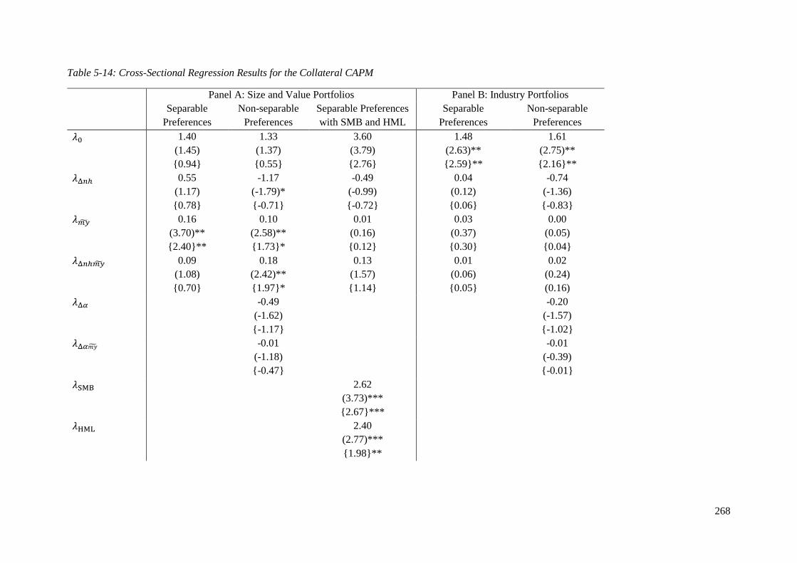
268

Table 5-14: Cross-Sectional Regression Results for the Collateral CAPM


Separable

Preferences

Non-separable

Preferences

Separable Preferences

with SMB and HML

Separable

Preferences

Non-separable

Preferences

𝜆0 1.40

(1.45)

{0.94}

1.33

(1.37)

{0.55}

3.60

(3.79)

{2.76}

1.48

(2.63)**

{2.59}**

1.61

(2.75)**

{2.16}**

𝜆Δ𝑛ℎ 0.55

(1.17)

{0.78}

-1.17

(-1.79)*

{-0.71}

-0.49

(-0.99)

{-0.72}

0.04

(0.12)

{0.06}

-0.74

(-1.36)

{-0.83}

𝜆𝑚�� 0.16

(3.70)**

{2.40}**

0.10

(2.58)**

{1.73}*

0.01

(0.16)

{0.12}

0.03

(0.37)

{0.30}

0.00

(0.05)

{0.04}

𝜆Δ𝑛ℎ𝑚�� 0.09

(1.08)

{0.70}

0.18

(2.42)**

{1.97}*

0.13

(1.57)

{1.14}

0.01

(0.06)

{0.05}

0.02

(0.24)

(0.16)

𝜆Δ𝛼 -0.49

(-1.62)

{-1.17}

-0.20

(-1.57)

{-1.02}

𝜆Δ𝛼𝑚�� -0.01

(-1.18)

{-0.47}

-0.01

(-0.39)

{-0.01}

𝜆SMB 2.62

(3.73)***

{2.67}***

𝜆HML 2.40

(2.77)***

{1.98}**

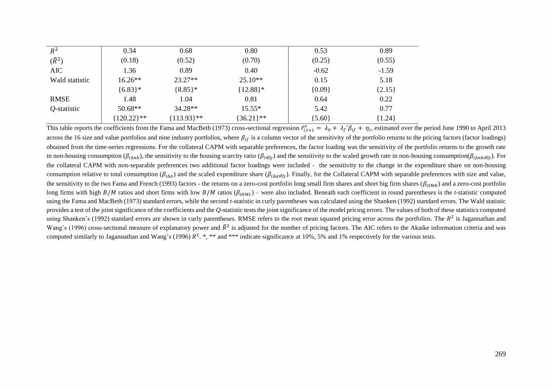
269

𝑅2

(��2)

0.34

(0.18)

0.68

(0.52)

0.80

(0.70)

0.53

(0.25)

0.89

(0.55)

AIC 1.36 0.89 0.40 -0.62 -1.59

Wald statistic 16.26**

{6.83}*

23.27**

{8.85}*

25.10**

{12.88}*

0.15

{0.09}

5.18

{2.15}

RMSE 1.48 1.04 0.81 0.64 0.22

Q-statistic 50.68**

{120.22}**

34.28**

{113.93}**

15.55*

{36.21}**

5.42

{5.60}

0.77

{1.24}



obtained from the time-series regressions. For the collateral CAPM with separable preferences, the factor loading was the sensitivity of the portfolio returns to the growth rate

in non-housing consumption (𝛽𝑖∆𝑛ℎ), the sensitivity to the housing scarcity ratio (𝛽𝑖𝑚��) and the sensitivity to the scaled growth rate in non-housing consumption(𝛽𝑖∆𝑛ℎ𝑚��). For

the collateral CAPM with non-separable preferences two additional factor loadings were included - the sensitivity to the change in the expenditure share on non-housing

consumption relative to total consumption (𝛽𝑖∆𝛼) and the scaled expenditure share (𝛽𝑖∆𝛼𝑚��). Finally, for the Collateral CAPM with separable preferences with size and value,

the sensitivity to the two Fama and French (1993) factors - the returns on a zero-cost portfolio long small firm shares and short big firm shares (𝛽𝑖𝑆𝑀𝐵) and a zero-cost portfolio

long firms with high 𝐵/𝑀 ratios and short firms with low 𝐵/𝑀 ratios (𝛽𝑖𝐻𝑀𝐿) – were also included. Beneath each coefficient in round parentheses is the t-statistic computed

using the Fama and MacBeth (1973) standard errors, while the second t-statistic in curly parentheses was calculated using the Shanken (1992) standard errors. The Wald statistic

provides a test of the joint significance of the coefficients and the Q-statistic tests the joint significance of the model pricing errors. The values of both of these statistics computed

using Shanken’s (1992) standard errors are shown in curly parentheses. RMSE refers to the root mean squared pricing error across the portfolios. The 𝑅2 is Jagannathan and

Wang’s (1996) cross-sectional measure of explanatory power and ��2 is adjusted for the number of pricing factors. The AIC refers to the Akaike information criteria and was

computed similarly to Jagannathan and Wang’s (1996) 𝑅2. *, ** and *** indicate significance at 10%, 5% and 1% respectively for the various tests.

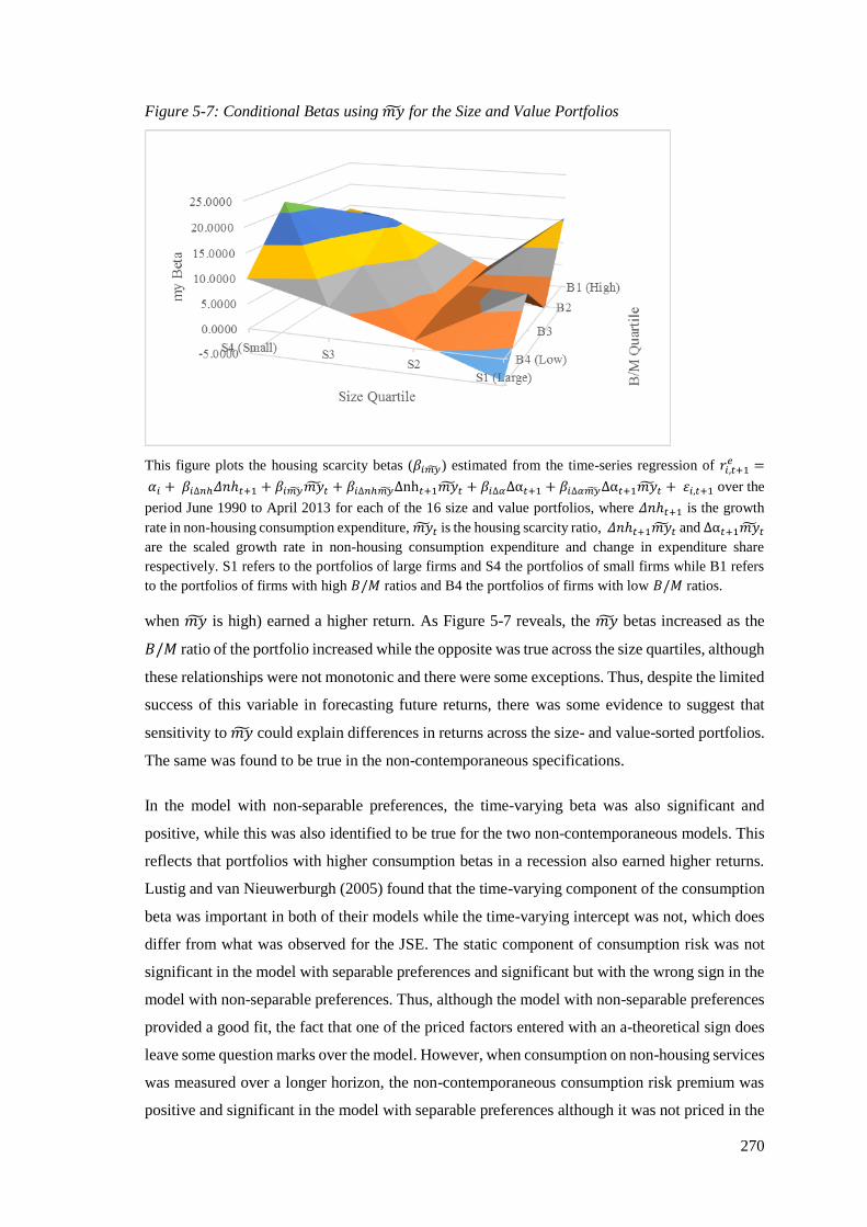
270

Figure 5-7: Conditional Betas using 𝑚�� for the Size and Value Portfolios

This figure plots the housing scarcity betas (𝛽𝑖𝑚��) estimated from the time-series regression of 𝑟𝑖,𝑡+1𝑒 =

𝛼𝑖 + 𝛽𝑖∆𝑛ℎ𝛥𝑛ℎ𝑡+1 + 𝛽𝑖𝑚��𝑚��𝑡 + 𝛽𝑖∆𝑛ℎ𝑚��Δnh𝑡+1𝑚��𝑡 + 𝛽𝑖∆𝛼Δα𝑡+1 + 𝛽𝑖∆𝛼𝑚��Δα𝑡+1𝑚��𝑡 + 휀𝑖,𝑡+1 over the

period June 1990 to April 2013 for each of the 16 size and value portfolios, where 𝛥𝑛ℎ𝑡+1 is the growth

rate in non-housing consumption expenditure, 𝑚��𝑡 is the housing scarcity ratio, 𝛥𝑛ℎ𝑡+1𝑚��𝑡 and Δα𝑡+1𝑚��𝑡

are the scaled growth rate in non-housing consumption expenditure and change in expenditure share

respectively. S1 refers to the portfolios of large firms and S4 the portfolios of small firms while B1 refers


when 𝑚�� is high) earned a higher return. As Figure 5-7 reveals, the 𝑚�� betas increased as the

𝐵/𝑀 ratio of the portfolio increased while the opposite was true across the size quartiles, although

these relationships were not monotonic and there were some exceptions. Thus, despite the limited

success of this variable in forecasting future returns, there was some evidence to suggest that

sensitivity to 𝑚�� could explain differences in returns across the size- and value-sorted portfolios.

The same was found to be true in the non-contemporaneous specifications.

In the model with non-separable preferences, the time-varying beta was also significant and

positive, while this was also identified to be true for the two non-contemporaneous models. This

reflects that portfolios with higher consumption betas in a recession also earned higher returns.

Lustig and van Nieuwerburgh (2005) found that the time-varying component of the consumption

beta was important in both of their models while the time-varying intercept was not, which does

differ from what was observed for the JSE. The static component of consumption risk was not

significant in the model with separable preferences and significant but with the wrong sign in the

model with non-separable preferences. Thus, although the model with non-separable preferences

provided a good fit, the fact that one of the priced factors entered with an a-theoretical sign does

leave some question marks over the model. However, when consumption on non-housing services

was measured over a longer horizon, the non-contemporaneous consumption risk premium was

positive and significant in the model with separable preferences although it was not priced in the

271

model with non-separable preferences, as shown in Table D-6 in the appendix. Similarly to those

collateral housing specifications analysed in the preceding section, in the collateral consumption

CAPM with non-separable preferences, the expenditure share was insignificant; thus favouring

the model with separable preferences albeit that the model with non-separable preferences had

higher explanatory power. This mirrors Lustig and van Nieuwerburgh’s (2005) findings, as

documented in section 5.2.3.2.

The Q-statistics showed that the pricing errors were significant across the size and value portfolios

for both models; however, consistent with the measures of explanatory power, the RMSE was

much lower for the model with non-separable preferences than that with separable preferences.

Lustig and van Nieuwerburgh (2005) also found that the pricing errors were significant for the

collateral consumption specifications but in contrast to this study, in their models, the RMSE was

lower on these models than the three-factor model. Figure 5-8 reveals that the portfolios with high

and low 𝐵/𝑀 ratios plotted further away from the 45-degree line indicating that the collateral

CAPM with non-separable preferences had some difficulty in explaining the returns to these

extreme shares.

Figure 5-8: Pricing Errors from the Collateral CAPM with Non-Separable Preferences for the

Size and Value Portfolios

This figure plots the pricing errors from the cross-sectional regression ��𝑖,𝑡+1𝑒 = 𝜆0 + 𝜆Δ𝑛ℎ𝛽𝑖∆𝑛ℎ +

𝜆𝑚��𝛽𝑖𝑚�� + 𝜆Δ𝑛ℎ𝑚��𝛽𝑖∆𝑛ℎ𝑚�� + 𝜆Δ𝛼𝛽𝑖∆𝛼 + 𝜆Δ𝛼𝑚��𝛽𝑖∆𝛼𝑚�� + 𝜂𝑖 over the period June 1990 to April 2013

across the 16 size and value portfolios, where 𝛽𝑖∆𝑛ℎ, 𝛽𝑖𝑚�� , 𝛽𝑖∆𝑛ℎ𝑚��, 𝛽𝑖∆𝛼and 𝛽𝑖∆𝛼𝑚�� measure the sensitivity

of the portfolio returns to the growth rate in non-housing consumption, the housing scarcity ratio, the scaled

growth rate in non-housing consumption, the change in the expenditure share on non-housing consumption

relative to total consumption, and the scaled change in expenditure share respectively. S1 refers to the

portfolios of large firms and S4 the portfolios of small firms while B1 refers to the portfolios of firms with

high 𝐵/𝑀 ratios and B4 the portfolios of firms with low 𝐵/𝑀 ratios.

272

Given that these collateral models appeared to be able to explain some of the pricing anomalies,

an additional test of the validity of the model with separable preferences was evaluated by

including SMB and HML as factors in the pricing equation. The results, also shown in Table 5-

14, indicate that the two Fama and French (1993) factors retained their significance and crowded

out the effects of the time-varying intercept and slope coefficient. Thus, although the pricing

factors in Lustig and van Nieuwerburgh’s (2005) model did have some explanatory power on the

JSE, SMB and HML still contain more information about the size- and value-sorted portfolios.

The ��2 measure of 70% is largely equivalent to that obtained in chapter 3 for the three-factor

model on the JSE, showing that the additional parameters added little value.

The findings for the industry portfolios reflect much the same patterns as noted under previous

specifications as none of the explanatory variables were significant. Therefore, although the

collateral CAPM had some success in explaining the returns across the size- and value-sorted

portfolios, the same was not true for the industry portfolios.


The final tests of the collateral CAPM was conducted in the GMM framework, with the results

thereof documented in Table 5-15. These results are largely identical to those obtained in the

cross-sectional regressions, as has largely been the case with the other models examined using

both approaches, but some small differences were noted. For example, for the industry-sorted

portfolios, the change in the expenditure share was priced in the cross-section; a result which is

identical to that observed in the CH-CAPM in the previous section. For the size- and value-sorted

portfolios, the time-varying intercept and time-varying slope coefficients were both found to be

significant in both the models with separable and non-separable preferences. This suggests that

returns on these portfolios and their measures of risk (their non-housing consumption betas) vary

across business cycles, with business cycles captured by 𝑚��. The expenditure share was found to

be significant in both the SDF and return-beta equation but the negative risk premium was

inconsistent with theory and the finding for the industry-sorted portfolios. But, this was similar to

that observed in testing the model of Piazzesi et al. (2003) in the previous section. The non-

housing consumption beta, although identified to be important in pricing securities in the presence

of the other factors in the SDFs, were priced with the incorrect sign. Despite some success with

identifying important pricing factors, the pricing errors of these models were significant.

The significance of 𝑚�� in the collateral consumption models confirms that housing wealth does

play an important role in business cycle risk for South African investors. Furthermore, the fact

that this ratio also considers labour income confirms some of the observations in chapter 4 that

labour income influences how individuals respond to consumption and investments.

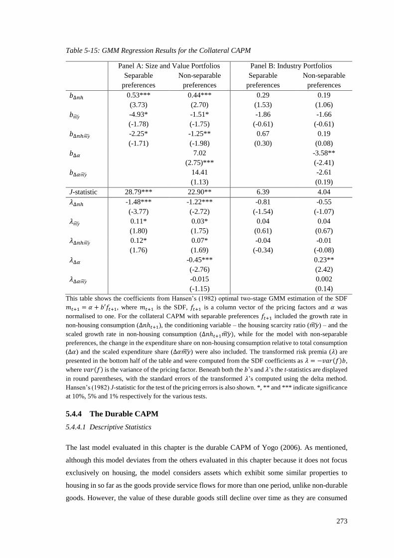
273

Table 5-15: GMM Regression Results for the Collateral CAPM


Separable

preferences

Non-separable

preferences

Separable

preferences

Non-separable

preferences

𝑏Δ𝑛ℎ 0.53***

(3.73)

0.44***

(2.70)

0.29

(1.53)

0.19

(1.06)

𝑏𝑚�� -4.93*

(-1.78)

-1.51*

(-1.75)

-1.86

(-0.61)

-1.66

(-0.61)

𝑏Δ𝑛ℎ𝑚�� -2.25*

(-1.71)

-1.25**

(-1.98)

0.67

(0.30)

0.19

(0.08)

𝑏Δ𝛼 7.02

(2.75)***

-3.58**

(-2.41)

𝑏Δ𝛼𝑚�� 14.41

(1.13)

-2.61

(0.19)

J-statistic 28.79*** 22.90** 6.39 4.04

𝜆Δ𝑛ℎ -1.48***

(-3.77)

-1.22***

(-2.72)

-0.81

(-1.54)

-0.55

(-1.07)

𝜆𝑚�� 0.11*

(1.80)

0.03*

(1.75)

0.04

(0.61)

0.04

(0.67)

𝜆Δ𝑛ℎ𝑚�� 0.12*

(1.76)

0.07*

(1.69)

-0.04

(-0.34)

-0.01

(-0.08)

𝜆Δ𝛼 -0.45***

(-2.76)

0.23**

(2.42)

𝜆Δ𝛼𝑚�� -0.015

(-1.15)

0.002

(0.14)



normalised to one. For the collateral CAPM with separable preferences 𝑓𝑡+1 included the growth rate in

non-housing consumption (∆𝑛ℎ𝑡+1), the conditioning variable – the housing scarcity ratio (𝑚��) – and the

scaled growth rate in non-housing consumption (∆𝑛ℎ𝑡+1𝑚��), while for the model with non-separable

preferences, the change in the expenditure share on non-housing consumption relative to total consumption

(Δ𝛼) and the scaled expenditure share (Δ𝛼𝑚��) were also included. The transformed risk premia (𝜆) are



in round parentheses, with the standard errors of the transformed 𝜆’s computed using the delta method.

Hansen’s (1982) J-statistic for the test of the pricing errors is also shown. *, ** and *** indicate significance

at 10%, 5% and 1% respectively for the various tests.

5.4.4 The Durable CAPM

5.4.4.1 Descriptive Statistics

The last model evaluated in this chapter is the durable CAPM of Yogo (2006). As mentioned,

although this model deviates from the others evaluated in this chapter because it does not focus

exclusively on housing, the model considers assets which exhibit some similar properties to

housing in so far as the goods provide service flows for more than one period, unlike non-durable

goods. However, the value of these durable goods still decline over time as they are consumed

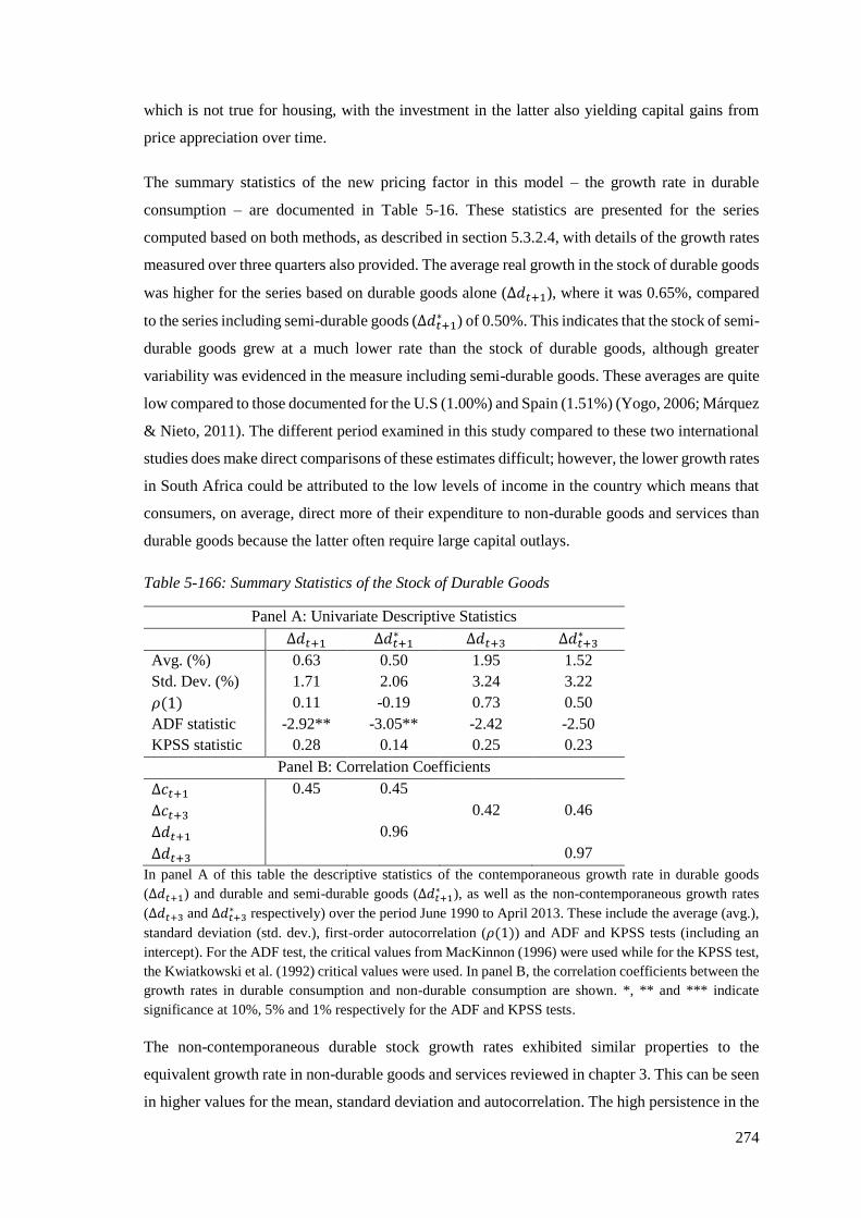
274

which is not true for housing, with the investment in the latter also yielding capital gains from

price appreciation over time.

The summary statistics of the new pricing factor in this model – the growth rate in durable

consumption – are documented in Table 5-16. These statistics are presented for the series

computed based on both methods, as described in section 5.3.2.4, with details of the growth rates

measured over three quarters also provided. The average real growth in the stock of durable goods

was higher for the series based on durable goods alone (∆𝑑𝑡+1), where it was 0.65%, compared

to the series including semi-durable goods (∆𝑑𝑡+1∗ ) of 0.50%. This indicates that the stock of semi-

durable goods grew at a much lower rate than the stock of durable goods, although greater

variability was evidenced in the measure including semi-durable goods. These averages are quite

low compared to those documented for the U.S (1.00%) and Spain (1.51%) (Yogo, 2006; Márquez

& Nieto, 2011). The different period examined in this study compared to these two international

studies does make direct comparisons of these estimates difficult; however, the lower growth rates

in South Africa could be attributed to the low levels of income in the country which means that

consumers, on average, direct more of their expenditure to non-durable goods and services than

durable goods because the latter often require large capital outlays.

Table 5-166: Summary Statistics of the Stock of Durable Goods


∆𝑑𝑡+1 ∆𝑑𝑡+1∗ ∆𝑑𝑡+3 ∆𝑑𝑡+3

∗

Avg. (%) 0.63 0.50 1.95 1.52

Std. Dev. (%) 1.71 2.06 3.24 3.22

𝜌(1) 0.11 -0.19 0.73 0.50

ADF statistic -2.92** -3.05** -2.42 -2.50

KPSS statistic 0.28 0.14 0.25 0.23


∆𝑐𝑡+1 0.45 0.45

∆𝑐𝑡+3 0.42 0.46

∆𝑑𝑡+1 0.96

∆𝑑𝑡+3 0.97

In panel A of this table the descriptive statistics of the contemporaneous growth rate in durable goods

(∆𝑑𝑡+1) and durable and semi-durable goods (∆𝑑𝑡+1∗ ), as well as the non-contemporaneous growth rates

(∆𝑑𝑡+3 and ∆𝑑𝑡+3∗ respectively) over the period June 1990 to April 2013. These include the average (avg.),

standard deviation (std. dev.), first-order autocorrelation (𝜌(1)) and ADF and KPSS tests (including an

intercept). For the ADF test, the critical values from MacKinnon (1996) were used while for the KPSS test,

the Kwiatkowski et al. (1992) critical values were used. In panel B, the correlation coefficients between the

growth rates in durable consumption and non-durable consumption are shown. *, ** and *** indicate

significance at 10%, 5% and 1% respectively for the ADF and KPSS tests.

The non-contemporaneous durable stock growth rates exhibited similar properties to the

equivalent growth rate in non-durable goods and services reviewed in chapter 3. This can be seen

in higher values for the mean, standard deviation and autocorrelation. The high persistence in the

275

series was confirmed in the ADF tests which indicated that the null hypothesis of a unit root could

not be rejected. However, the results from the KPSS tests yielded a contradictory conclusion that

both measures could be considered stationary. Such inconsistencies between the ADF and KPSS

tests are likely to arise when the root of the characteristic equation likes close to one (which was

the case with these two growth rates) in which case the ADF test is seen to have low power. This

frequently results in the failure to reject the null hypothesis. Accordingly, the conclusions

provided by the KPSS tests were relied upon for this purpose as they do not have the same low

power problem. As such, these growth rates were viewed as stationary and could be used as

pricing factors in the durable CAPM.


Although minor differences were evident in the properties of the growth rates in durable stock

based on the two methods used, the two series were highly correlated with a coefficient of 0.96,

as shown in Table 5-16. Semi-durable goods thus moved closely over time with durable goods

and in addition to this, the method used to obtain a starting point for the stock of durable

consumption provided a good approximation of the implied durable stock value obtained from

the SARB memo item. Only the results for the models using the measure including semi-durable

goods, ∆𝑑∗, are reported, with those based on the growth rate in durable goods alone, ∆𝑑,

presented in Table D-7 in the appendix (p. 340), as the two methods yielded largely identical

results. Although the results in panel B of Table 5-16 also indicate that consumption on durable

goods and non-durable goods and services were quite closely correlated, it was not considered

necessary to orthogonalise the durable growth rate as the correlation was less than the cut-off of

0.5.

The two durable CAPM specifications were able to explain 27% and 42% of the cross-sectional

variation of the size and value portfolios, as shown in Table 5-17, with the non-contemporaneous

model yielding the higher ��2as well as the lower AIC. The explanatory power of the non-

contemporaneous durable CAPM is slightly lower than the collateral CAPM based on non-

separable preferences (52%) obtained previously but exceeds that of many of the labour-income

based specifications analysed in chapter 4. Although Yogo (2006) found that the model was able

to explain 94% of the variation in the cross-section of size and value portfolio returns; when using

portfolios of U.S shares sorted based on size and industry, Márquez and Nieto (2011) documented

much lower ��2 values of 53% and 58% for the contemporaneous and non-contemporaneous

models respectively. For the Spanish market, these authors found that both models were able to

explain approximately 50% of the variation across size-sorted portfolios. Thus, the durable

CAPM does not appear to be able to explain as much of the variation in the cross-section of South

African share returns as for the U.S and Spain.

276

Table 5-17: Cross-Sectional Regression Results for the Durable CAPM with ∆𝑑∗


Durable CAPM Non-contemporaneous

Durable CAPM

Non-contemporaneous

Durable CAPM with

Size and Value


Durable CAPM

𝜆0 7.04

(4.51)**

{3.07}**

5.98

(3.83)**

{2.94}**

3.65

(1.98)*

{1.66}

3.86

(4.36)**

{4.11}**

2.94

(2.00)**

{1.91}**

𝜆𝑚 -6.70

(-3.17)**

{-2.15}**

-4.77

(-2.29)**

{-1.75}*

-3.01

-1.27

-1.07

-2.97

(-1.31)

{-0.74}

-1.75

(-0.71)

{-0.42}

𝜆∆𝑐𝑡+1 0.84

(1.81)*

{1.22}

0.03

(0.09)

{0.05}

𝜆Δ𝑑 -0.61

(-0.94)

{-0.64}

0.20

(0.35)

{0.21}

𝜆Δ𝑐𝑡+3 0.13

(0.19)

{0.15}

0.51

(0.78)

{0.65}

0.11

(0.21)

{0.10}

𝜆Δ𝑑𝑡+3 1.21

(2.53)**

{1.92}*

0.17

(0.24)

{0.20}

0.49

(0.51)

{0.33}

𝜆SMB 2.83

(3.87)***

{3.19}***

𝜆HML 2.43

(2.80)***

277

{2.31}**

��2 0.41

(0.27)

0.53

(0.42)

0.74

(0.61)

0.75

(0.60)

0.68

(0.49)

AIC 1.24 1.06 0.72 -1.08 -1.08


{6.52}*

11.68***

{6.80}*

25.11***

{17.10}**

1.90

{0.60}

0.81

{0.30}

RMSE 1.40 1.28 0.95 0.44 0.42

Q-statistic 40.83**

{88.54}**

38.25**

{64.85}**

16.23*

{38.95}**

3.90

{4.39}

3.74

{4.11}



obtained from the time-series regressions. For the durable CAPM, the factor loadings were the sensitivity to the growth rate in non-durable consumption (𝛽𝑖∆𝑐), durable

consumption (𝛽𝑖∆𝑑∗) (where growth in durable goods also included semi-durable goods, denoted ∆𝑑∗) and the excess real market returns (𝛽𝑖𝑚). For the non-contemporaneous

specification, the factor loadings are identical but are measured relative to the non-contemporaneous growth rates (measured over three quarters) on durable and non-durable

consumption respectively. Finally, for the non-contemporaneous model with size and value, the sensitivity to the two Fama and French (1993) factors - the returns on a zero-

cost portfolio long small firm shares and short big firm shares (𝛽𝑖𝑆𝑀𝐵) and a zero-cost portfolio long firms with high 𝐵/𝑀 ratios and short firms with low 𝐵/𝑀 ratios (𝛽𝑖𝐻𝑀𝐿) –

were also included. Beneath each coefficient in round parentheses is the t-statistic computed using the Fama and MacBeth (1973) standard errors, while the second t-statistic in

curly parentheses was calculated using the Shanken (1992) standard errors. The Wald statistic provides a test of the joint significance of the coefficients and the Q-statistic tests

the joint significance of the model pricing errors. The values of both of these statistics computed using Shanken’s (1992) standard errors are shown in curly parentheses. RMSE

refers to the root mean squared pricing error across the portfolios. The 𝑅2 is Jagannathan and Wang’s (1996) cross-sectional measure of explanatory power and ��2 is adjusted

for the number of pricing factors. The AIC refers to the Akaike information criteria and was computed similarly to Jagannathan and Wang’s (1996) 𝑅2. *, ** and *** indicate

significance at the 10%, 5% and 1% levels respectively for the various tests.

278

Similarly to most specifications examined in this study, the intercepts were significant and the

estimated market risk premium was significant but with a negative coefficient. The inclusion of

the two consumption factors in the pricing equation therefore did not salvage the market beta as

a pricing factor in explaining the cross-section of share returns. The results of the durable CAPM

on the South African market differ from the international findings, as although Yogo (2006)

obtained an insignificant market risk premium for the U.S, Márquez and Nieto (2011) found the

premium to be positive and significant for Spanish shares.

The risk premium associated with consumption on non-durable goods and services was significant

but only at 10% and was insignificant in the non-contemporaneous model when the betas were

measured relative to a three-quarter rather than a single quarter growth rate. The finding of only

a limited role for consumption in the pricing of the cross-section of securities on the JSE is broadly

consistent with the results obtained for other models in this study, especially in the presence of

other significant pricing factors. Yogo (2006) and Márquez and Nieto (2011) found that the non-

durable consumption beta was insignificant in their tests on the U.S and Spanish markets,

although for the latter there was some evidence that this factor was important when consumption

was measured over a longer horizon.

When durable consumption was measured over a one-quarter horizon, the risk premium on the

durable beta was insignificant (and entered with the wrong sign). But, as indicated in Table 5-17,

when the growth rate was measured over a three-quarter horizon, the durable beta was priced with

a positive risk premium. This finding that it is the non-contemporaneous durable beta that plays

an important role in the pricing specification mirrors that of Márquez and Nieto (2011) for the

Spanish market. To examine the role of this factor in explaining returns across the size and value

portfolios more closely, a graph of the non-contemporaneous durable betas is shown in Figure 5-

9. These betas appear to capture the size premium quite well as portfolios comprising small firms

were those with higher durable betas. As mentioned in section 5.2.4, growth in durable goods is

likely to be low when the market is low and thus firms which are highly correlated with the growth

rate in durable goods are pro-cyclical meaning that they deliver low returns when the market is

already low. As such, investors demand a high premium for holding these shares. In some cases,

the portfolios of larger firms exhibited negative durable betas showing that these firms represented

a hedge as they moved counter-cyclically. Márquez and Nieto (2011) also found that the durable

betas could explain some of the size premium on the Spanish market. Turning to the patterns

across the 𝐵/𝑀 groupings, the durable betas were higher for the value portfolios but only in the

two smallest quartiles and thus this factor had less success in explaining the value premium

compared to the size premium. This conclusion differs from Yogo (2006) who found substantive

evidence that the value shares were more sensitive to durable consumption growth.

279

Figure 5-9: Non-Contemporaneous Durable Consumption Betas Based on ∆𝑑∗for the Size and

Value Portfolios

This figure plots non-contemporaneous durable betas (𝛽𝑖∆𝑑) estimated from the time-series regression of

𝑟𝑖,𝑡+1𝑒 = 𝛼𝑖 + 𝛽𝑖∆𝑐𝛥𝑐𝑡+3 + 𝛽𝑖∆𝑐𝛥𝑑𝑡+3 + 𝛽𝑖𝑚𝑟𝑚,𝑡+1

𝑒 + 휀𝑖,𝑡+1 over the period June 1990 to April 2013 for

each of the 16 size and value portfolios, where 𝛥𝑐𝑡+3 is the non-contemporaneous growth rate in

consumption on non-durable goods and services, 𝛥𝑑𝑡+3 is the non-contemporaneous growth rate in durable

consumption (both measured over three quarters) and 𝑟𝑚,𝑡+1𝑒 is the excess real market returns. S1 refers to

the portfolios of large firms and S4 the portfolios of small firms while B1 refers to the portfolios of firms


Examining the pricing errors of the model, the non-contemporaneous model yielded lower errors,

on average, than the contemporaneous model; but, similarly to the other models examined in this

study, the pricing errors were significant. This is confirmed in Figure 5-10, which shows the

pricing errors from the non-contemporaneous durable CAPM for the 16 size and value portfolios.

Consistent with the patterns observed in Figure 5-10, the model had particular difficulty in

explaining the returns to the portfolios comprising high 𝐵/𝑀 ratios (where the fitted returns were

too low compared to the actual returns) and low 𝐵/𝑀 ratios (where the fitted returns were too

high compared to the actual returns). Although the model was able to capture some of the size

premium, it had difficulty in explaining the returns to the portfolios of the ‘very small’ shares.

For the industry-sorted portfolios, again, none of the slope coefficients were significant. As

mentioned, Márquez and Nieto (2011) did utilise industry-sorted portfolios in their tests but

because they combined these with their size-sorted specifications, it makes it difficult to directly

compare their results to those obtained here which rely only on sorting shares according to

industry classifications.

280

Figure 5-10: Pricing Errors from the Non-Contemporaneous Durable CAPM with ∆𝑑∗for the

Size and Value Portfolios

This figure plots the pricing errors from the cross-sectional regression ��𝑖,𝑡+1𝑒 = 𝜆0 + 𝜆Δ𝑐𝛽𝑖∆𝑐 + 𝜆Δ𝑑𝛽𝑖∆𝑑 +

𝜆𝑚𝛽𝑖𝑚 over the period June 1990 to April 2013 across the 16 size and value portfolios, where 𝛽𝑖∆𝑐, 𝛽𝑖∆𝑑

and 𝛽𝑖𝑚 measure the sensitivity of the portfolio returns to the growth rate in non-contemporaneous non-

durable and durable consumption and the excess real market returns respectively. S1 refers to the portfolios

of large firms and S4 the portfolios of small firms while B1 refers to the portfolios of firms with high 𝐵/𝑀

ratios and B4 the portfolios of firms with low 𝐵/𝑀 ratios.

Given that the non-contemporaneous durable CAPM had some success in explaining the size

anomaly, this model was evaluated further by examining whether the two Fama and French (1993)

factors – size and value – were still priced when combined with the other pricing factors in this

model. The results, shown in Table 5-17, indicate that size and value still give rise to positive and

significant risk premia while that associated with non-durable consumption becomes

insignificant. Accordingly, although correlation with durable goods can account for some of the

size anomaly on the JSE, it does not entirely explain why small firms earned higher returns than

large firms such that the size factor is still an important term in pricing the cross-section of size

and value portfolios.


As a final test of the durable CAPM, the model was estimated using GMM. The results thereof,

presented in Table 5-18, provide conclusions which are largely consistent with those obtained

from the cross-sectional regressions, although some minor differences were noted. The market

risk premium in both the contemporaneous and non-contemporaneous specifications was negative

281

Table 5-18: GMM Regression Results for the Durable CAPM with ∆𝑑∗


Durable CAPM Non-

contemporaneous

Durable CAPM

Durable CAPM Non-

contemporaneous

Durable CAPM

𝑏𝑚 0.01

(0.61)

0.01

(0.64)

0.01

(0.71)

-0.00

(-0.03)

𝑏∆𝑐 -0.81***

(-2.67)

0.20

(0.49)

𝑏Δ𝑑 0.19

(0.76)

-0.19

(-0.74)

𝑏Δ𝑐𝑡+3 -0.06

(-0.69)

0.02

(0.21)

𝑏Δ𝑑𝑡+3 -0.20**

(-2.45)

-0.13

(-1.28)

J-statistic 40.29*** 30.77*** 8.24 4.85

𝜆𝑚 -0.76

(-0.66)

-0.82

(-0.65)

-1.19

(-0.72)

0.05

(0.03)

𝜆∆𝑐 1.92***

(2.70)

-0.47

(-0.50)

𝜆Δ𝑑 -0.79

(-0.77)

-0.80

(-0.75)

𝜆Δ𝑐𝑡+3 0.49

(0.70)

-0.19

(-0.21)

𝜆Δ𝑑𝑡+3 2.10**

(2.48)

1.39

(1.29)



normalised to one. For the durable CAPM, 𝑓𝑡+1 included the one quarter growth rates in non-durable

(∆𝑐𝑡+1) and durable (Δ𝑑𝑡+1∗ ) consumption with ∆𝑑∗ referring to the measure which included both durable

and semi-durable goods. For the non-contemporaneous durable CAPM both the non-durable (∆𝑐𝑡+1) and

durable (Δ𝑑𝑡+3∗ ) growth rates were computed over three-quarters. The transformed risk premia (𝜆) are



in round parentheses, with the standard errors of the transformed 𝜆’s computed using the delta method.

Hansen’s (1982) J-statistic for the test of the pricing errors is also shown. *, ** and *** indicate significance

at the 10%, 5% and 1% levels respectively for the various tests.

but insignificant contrary to the cross-sectional regression results where it had the same sign but

was significant. Consumption on non-durable goods and services was insignificant in the cross-

sectional regression whereas for the GMM results this factor was important in helping to price

securities in the SDF and it was priced in the return-beta model. The non-contemporaneous

growth rate in the second model, however, was still insignificant based on the GMM results.

Similarly to the results presented in the previous section, a significant role for durable

282

consumption in pricing securities was only identified when measured over the three-quarter

horizon and not over the single quarter horizon. Despite some factors in these two models being

priced, both yielded pricing errors which were significant, as captured by the J-statistics. For the

industry portfolios, none of the coefficients were significant in either the SDF or return-beta

equation as shown in panels A and B of Table 5-18.

Overall, the results suggest that the durable CAPM can explain some patterns in share returns,

but certainly not all. While the durable growth rate is priced in the cross-section, the negative

market risk premium calls into question the suitability of this model. Thus, while Yogo (2006)

contended that his model provided a superior specification to previous models such as Lettau and

Ludvigson (2001b), Lustig and van Nieuwerburgh (2005) and Parker and Julliard (2005), the

evidence for South Africa, consistent with that documented by Márquez and Nieto (2011) for both

the Spanish and U.S markets, indicates that this model is not the solution to the asset pricing

puzzle.

5.5 CONCLUSION

The wealth arising from housing is multifaceted as it includes the capital gain component

associated with other investment assets, but also provides consumption in the form of housing

services. Both of these components of housing wealth are likely to be correlated with consumption

patterns over time as the returns from the investment in housing can be used to finance

expenditure on goods and services, while investors can substitute consumption of housing

services for non-housing goods and services. Housing wealth thus directly feeds into the

association between share returns and consumption, as human capital was also observed to do.

Piazzesi et al. (2007), Lustig and van Nieuwerburgh (2005) and Sousa’s (2010) derived measures,

which capture this interrelationship, have been found to predict share returns in the U.S.

The consumption CAPM should reflect any risk arising from housing wealth but because proxies

for consumption are used they may not provide an accurate reflection of this relationship. Using

the composite variables that link consumption and housing wealth as conditioning variables in

the conditional CAPM and (C)CAPM, Piazzesi et al. (2003) and Lustig and Van Nieuwerburgh

(2005) showed that these models could explain some of the premia associated with small firms

and those with low 𝐵/𝑀 ratios. Yogo’s (2006) durable CAPM focuses on goods that provide

services for more than one period, but which still depreciate in value with usage, unlike housing,

had similar success. These models were tested on the JSE to assess their ability to explain the

283

cross-section of share returns in an emerging market along with a simple real estate augmented

CAPM.

In the real estate CAPM, residential real estate returns were found to be priced with the positive

risk premium confirming that securities which were more closely correlated with the returns from

residential real estate yielding higher returns. In particular, small firms were found to have large

factor loadings suggesting that because these securities moved closely with the real estate wealth

of investors they did not provide as much utility as large shares which moved less closely (or even

negatively) with real estate wealth. Turning to the models which used composite measures to

consider the impact of housing wealth with consumption (and in some cases labour income as

well), some success was observed, most notably in the collateral CAPM and conditional CH-

CAPM, where the coefficients on the time-varying intercepts were positive and significant. Thus,

𝛼 and 𝑚�� were both able to document how returns for the size- and value-sorted portfolios varied

over business cycles as the composition risk of consumption (consumption of non-housing

services relative to housing services) and the housing collateral ratio (the amount of housing

wealth and labour income used to support consumption expenditure) varied. Moreover, the former

was found to have greater explanatory power for the size anomaly and the latter for the value

anomaly. The durable CAPM of Yogo (2006) also yielded a substantial role for durable

consumption (allied to the size anomaly), when measured over a three-quarter horizon. This

confirms that expenditure on goods which provide service flows for more than one period is an

important determinant of share returns.

Some of the evidence documented was found to be consistent with the patterns identified in the

U.S, but in many instances differences were evident; such as the time-varying returns being

significant for the South African sample rather than the time-varying risk measures in the U.S.

Several notable differences, however, were observed including the fact that despite some success

in identifying significant pricing factors, the pricing errors remained significant across all the

specifications examined, the explanatory power of the models was lower than the Fama and

French (1993) three-factor model, and SMB and HML were priced and largely crowded out the

effects of the other variables when added into these models. The latter highlights the dominance

of these pricing factors in explaining the returns across the size and value portfolios. None of the

models had any ability to account for the industry-sorted portfolios.

Although the models of Piazzesi et al. (2003), Lustig and van Nieuwerburgh (2005) and Yogo

(2006) were found to be successful in accounting for the anomalies on the U.S market, the South

African evidence was less convincing as the models were able to explain some, but not all, of the

284

cross-sectional variation. The use of an aggregate measure for consumption which incorporates

the expenditure of a large component of non-investors may explain the differences across the U.S

and South African markets, while the measures of housing value may also be subject to some

limitations given the data constraints that were faced. Certainly, however, there is sufficient

evidence to suggest that the relationship between consumption and share returns is affected by

both housing and human capital wealth but that none of the models examined provides a

comprehensive asset pricing model for the emerging South African market.

In the following chapter, a summary of the key findings of this study are reported in the context

of the research objectives outlined in chapter one. Thereafter, recommendations for future

research are provided in light of the findings of the various analyses conducted.

285

Chapter 6 : CONCLUSIONS AND RECOMMENDATIONS

6.1 INTRODUCTION

This chapter draws this study to completion. A review of the background to the study is provided,

including the research question, which was the subject of attention. Thereafter the findings

pertaining to each research objective are briefly examined and conclusions drawn. The limitations

of the study are highlighted and, finally, recommendations for future research are provided.

6.2 A REVIEW OF THE PROBLEM STATEMENT

It is a well-established fact that some shares earn higher returns than others, with the higher returns

seen as compensation for greater risk. What is less clear, however, is what factors determine risk.

The CAPM of Sharpe (1964) and Lintner (1965a), building from Markowitz’s (1952) MPT,

dramatically changed the face of risk measurement by providing an intuitive and simple measure

of risk, known as beta. Beta only captures systematic risk as investors need not be compensated

for the part of firm risk that can be eliminated through the construction of a diversified portfolio.

But the assumptions underlying the model are regarded as limiting because they do not represent

the realities of investing. Moreover, a plethora of evidence has been documented which reveals

that the positive risk-return relationship postulated by the CAPM does not hold in practice (the

relationship is, at best, flat), while the model also cannot explain numerous anomalous patterns

in returns – most notably the higher risk-adjusted returns earned by small firms and firms with

high 𝐵/𝑀 ratios compared to large firms and firms with low 𝐵/𝑀 ratios respectively. Further

criticism of the model lies in the fact that the CAPM reveals little about what actually determines

share prices because risk is measured relative to the returns on a portfolio of securities, with no

indication as to what determines the returns of the securities in the portfolio used to price other

securities!

In response to these weaknesses of the CAPM, numerous other asset pricing models have been

developed. They can largely be grouped into two categories – portfolio-based models and

macroeconomic-based models. Models which fit into the former category can be seen as

extensions to the CAPM, as they focus on measuring risk by the sensitivity of share returns to a

set of synthesised portfolios. In contrast, macroeconomic-based models seek to identify what

macroeconomic variables determine share prices, given that share prices are affected by external

286

forces. This distinction is less than clear-cut, of course, as new research continually challenges

the boundaries between the groupings.

Several theoretical and empirical portfolio-based models have been developed. One theoretical

model which has made a substantial contribution to the literature is the conditional CAPM of

Jagannathan and Wang (1996) and Lettau and Ludvigson (2001b). This model relaxes the one-

period time horizon of the CAPM and yields a framework that allows for both risk and returns to

vary over time, with this time-variation linked to forecasted changes in the business cycle.

Although the success of the model in explaining the size and value anomalies has been limited,

and it does not directly provide information about what factors drive share returns, the conditional

CAPM does provide a link to the macroeconomy through variations in business cycles. Moreover,

the time-varying nature of the model is considered substantially more realistic than the original

static framework. At the other end of the spectrum of portfolio-based models is the three-factor

model of Fama and French (1993), which was derived directly as a consequence of the empirical

evidence on the size and value anomalies. This model expands the CAPM by measuring the risk

of a security not only relative to the market portfolio but also to two synthesised portfolios created

so as to capture the higher returns associated with small compared to large firms and value

compared to growth firms. This model has achieved notable success empirically, to the extent

that its performance is viewed as the benchmark against which other asset pricing models are

compared. However, the three-factor model provides no information about what factors truly

drive share returns, with the size and value portfolios simply proxying for risks not identified.

At the heart of the macroeconomic approach to asset pricing is the consumption CAPM, which

links the utility derived from consumption to share returns. The APT, by contrast, not only leaves

the macroeconomic factors ‘unidentified’ but also only looks at the direct impact of the

macroeconomic variables on share returns as opposed to how it influences the behaviour of

investors. However, the consumption CAPM has performed as poorly, if not worse, than the

standard CAPM in empirical tests. One explanation that has been proposed to account for this

poor performance is that aggregate consumption is not observable and thus the proxies used may

not fully capture all risks inherent in consumption. Human capital and housing wealth have both

been shown to influence consumption patterns over time, which in turn affects the rewards

investors demand from investing. Several asset pricing models (such as Lettau & Ludvigson,

2001b; Lustig & van Nieuwerburgh, 2005) have been developed to account for these relationships

that may not be fully captured in the consumption measure used in the consumption CAPM. This

is achieved by taking into consideration how these variables interact across different business

287

cycles and thus the models also allow for time-varying risk and return (as per the conditional

CAPM). The empirical tests of these models have shown that when such dynamics between labour

income, consumption and housing wealth are accounted for in the asset pricing models, the size

and value premia are notably reduced. These results thus point to a substantial role for both labour

income and housing wealth in the pricing of securities.

As mentioned in chapter 1, Cochrane (2005, pp. xiv) noted that the task of identifying

macroeconomic factors that drive share returns was unfinished. Although progress has been made

on this front over the past ten years, Cochrane’s (2005) comment is arguably still appropriate.

This can be seen in that not only has no single comprehensive model yet been identified that can

fully account for differences in returns across securities, but also because there is still very little

evidence of whether the determinants of share returns that have been identified in the U.S are as

important in other markets, especially those less developed and with differing institutions. The

goal of this research was thus to attempt to fill part of this gap and, in so doing, advance the work

on macroeconomic asset pricing. In particular, the focus was on ascertaining whether

macroeconomic models which link labour income and housing wealth to the consumption patterns

of investors, and thus their demand for securities, can help to explain share returns on the

emerging market of South Africa. Thus the attention was on identifying a model which performs

well and, in so doing, sheds light on the fundamental determinants of share returns.

6.3 SUMMARY OF FINDINGS

6.3.1 The CAPM, the Two-Factor Model and the Three-Factor Model

The time-series tests of the CAPM and van Rensburg’s (2002) two-factor model confirmed the

presence of the size and value anomalies on the JSE as the pricing errors associated with the

portfolios comprising small firms and firms with high 𝐵/𝑀 ratios were significant and positive.

The GRS joint test of significance validated this conclusion as the pricing errors were significant

for both models, with these results mirroring those of Basiewicz and Auret (2010). However,

when the Fama and French (1993) three-factor model was examined, the majority of the intercepts

were insignificant; a result confirmed by the GRS test. This latter finding did differ from that of

Basiewicz and Auret (2010), who found that the null hypothesis of the GRS test could be rejected

at 10%, as although the model could explain the value anomaly it had greater difficulty with the

high returns to small firms. The fact that the same was not true for this study was attributed to the

different methods employed in computing the SMB and HML factors. The method used in this

288

study compared to that of Basiewicz and Auret (2010) was likely to identify a more pronounced

size premium which is concentrated in the ‘very’ small shares on the JSE.

Although previous cross-sectional analyses of the CAPM on the JSE had revealed evidence of a

negative relationship between risk and return across portfolios sorted on the basis of size and

𝐵/𝑀, the results from this analysis not only confirmed this finding but identified that the

relationship was significant. Thus the results seemed to suggest that those shares which were more

highly correlated with the market earned lower returns - in complete contrast to the key principle

that higher risk should be compensated with higher returns. Negative and significant coefficients

were also observed on the two market proxies in the tests of van Rensburg’s (2002) model, which

was not surprising as these two factors simply represent a disaggregated market portfolio. Thus

although these two models were able to explain a larger proportion of the cross-sectional variation

(27% and 35% respectively) than has been observed for the CAPM in many international

countries, this explanatory power was driven by pricing factors with atheoretical coefficients.

Neither model produced significant pricing factors in the sample of industry-sorted portfolios.

The Fama and French (1993) three-factor model was able to explain 70% of the variation across

the size and value portfolios on the JSE, with both the SMB and HML factors carrying a

significant positive risk premium. However, the market risk premium, similarly to the CAPM,

was negative and significant. As Lewellen et al. (2010) pointed out, a model should be able to

explain all patterns in share returns, and on this front the three-factor model failed: although it

was able to explain 54% of the cross-sectional variation in the industry-sorted portfolios, none of

the pricing factors were significant. Moreover, although the model was able to explain a

substantial portion (but not all) of the size and value premia, the model has no way of detailing

exactly what factors drive share returns as SMB and HML are merely synthesised portfolios.

6.3.2 A Test of the Conditional CAPM on the JSE

Prior to testing the conditional CAPM, a review of the time-series predictability of the market

portfolio returns was conducted using several traditional forecasting variables. The results showed

that the relative T-bill yield and term spread had some predictive power but this was concentrated

at medium-term and short-term horizons respectively. The 𝐷/𝑃 and 𝐸/𝑃 ratios were found to

have limited forecasting power for future share returns, after adjusting for their persistent nature,

with the lagged market returns also containing no information about future share returns. The

findings regarding the term spread and relative T-bill were largely consistent with those of Gupta

and Modise (2012a, 2012b, 2013) for the South African market as were those observed for 𝐷/𝑃

289

and 𝐸/𝑃 despite differing methods of analysis, different frequencies of data and the differing time

periods reviewed.

Turning to the conditional CAPM, the models tested yielded relatively high ��2 values on the size

and value portfolios ranging between 29% and 66%. However, as with the CAPM, in four of the

five models, the market risk premium was significant and negative. The coefficient on the time-

varying beta was only significant for the model based on the term spread but this did yield a

positive coefficient consistent with the view that risk is higher during recessions. The coefficient

on the time-varying intercept was significant for 𝐷/𝑃, 𝐸/𝑃 and the lagged market risk premium,

but only the latter entered with the correct sign. The fact that the lagged market risk premium was

an important determinant of the cross-section of share returns initially appeared inconsistent with

the time-series forecasting regressions but, rather than capturing risk arising from variation in

returns across business cycles, this result appears to reflect that returns are a function of risk in

the previous period (i.e. there is a delayed positive risk-return relationship). This result is

consistent with the time-series findings of Basiewicz and Auret (2010). Although some surprising

results were obtained in the tests of the conditional CAPM on the JSE there was sufficient

evidence to indicate that the relationship between risk and return is dynamic and varies over

business cycles.

6.3.3 A Test of the Consumption CAPM on the JSE

The consumption CAPM performed as poorly on the JSE as internationally, with the ��2 from

both specifications estimated (a second specification was estimated with a three-period growth

rate in consumption rather than only a one-period rate) negative. Despite this negative explanatory

power, there was some weak evidence that the estimated positive risk premia were significant,

but an analysis of the consumption betas confirmed that there were few consistent patterns with

only a weak positive relationship between the measure of value and consumption. Largely,

however, these findings were consistent with the international evidence. As indicated in chapter

3, one limitation of the consumption CAPM is the fact that not all consumers are investors and

thus using total consumption measures may not be an appropriate means of capturing the

behaviour of investors. This may be exacerbated in South Africa as participation rates are likely

to be even lower given low income levels. Moreover, the fact that the market is dominated by

institutional investors also suggests that the utility derived by individual investors from their

investments may not necessarily be a driving force in share returns over time.

290

6.3.4 The Role of Labour Income in Explaining South African Share Returns

An initial analysis of the CAPM augmented with labour income yielded a negative relationship

between returns and labour income (which was significant in some instances). This finding does

differ from some of the international evidence as labour income carried a positive risk premium

in the Japanese market. Although the same was true for some periods in the U.S, the results from

the U.K and Australia of a limited or even negative role for labour income suggest that the

emerging market of South Africa is not necessarily unique.

The consumption aggregate wealth ratio, 𝑐𝑎𝑦, of Lettau and Ludvigson (2001b) was found to

have substantial forecasting power for JSE-listed shares over both short- and medium-term

horizons whereas the labour income-to-consumption measure, 𝑠𝑦, of Santos and Veronesi (2006)

contained no information about future share returns. The fact that both of these measures rely on

the interaction between labour income and consumption and yet give rise to contrasting results in

the forecasting regressions is surprising. However, 𝑐𝑎𝑦 also incorporates asset wealth which

suggests that this may be an important dynamic in examining the relationship on the South African

market. Aggregate measures of labour income and consumption reflect the activities of the

population and not exclusively investors and in South Africa, investors are likely to constitute

only a small component of the total population. However, through the introduction of asset wealth

into the measure the dynamics between labour income and consumption may be better captured

because asset wealth, although again an aggregate estimate, reflects changes to the wealthier

individuals’ positions. The same may also be true of institutional investors who may consider the

interaction between labour income, consumption and asset wealth as a more representative

measure than only the interaction between labour income and consumption.

For the tests of the conditional models using these two ratios, the results were broadly consistent

with the forecasting regressions, as the use of 𝑠𝑦 yielded some insignificant coefficients while

those that were significant - the market risk premium and the scaled market risk premium - were

negative. In contrast, the model of Lettau and Ludvigson (2001b) was found to have some

explanatory power for the South African market, with evidence to suggest that value shares earned

more because they were riskier during bad states when 𝑐𝑎𝑦 was high. But this model was not able

to explain all of the patterns in the returns, with the pricing errors significant and both SMB and

HML still priced in returns. This differed from the U.S market, but is similar to the findings for

Australia, suggesting that factors other than the interaction between labour income, consumption

and aggregate wealth explain share returns on the JSE. At the very least, however, this model

provided information to suggest that some of these macroeconomic variables that have been found

291

to be able to explain returns on developed markets are also applicable to developing markets –

which was one of the founding objectives of this study.

6.3.5 The Role of Housing Wealth in Explaining South African Share Returns

In chapter 5, the role of housing wealth in asset pricing was examined. As a starting point for this

analysis, the real estate CAPM, which examines the direct effect of the returns to real estate (not

only housing) on share returns, was tested. The risk premium on residential real estate (which can

be seen as a proxy for the returns to housing) was positive and significant, with the returns of

small shares more closely correlated with the returns from residential real estate; thus suggesting

some role for not only real estate, but more specifically, housing, in determining share returns on

the JSE.

At the heart of the analysis was the examination of the relationship between housing wealth,

consumption (as well as labour income in some cases) and share returns and the implications for

asset pricing. The ratios capturing this relationship were less successful than has been observed

in the U.S: the housing scarcity ratio, 𝑚��, of Lustig and van Nieuwerburgh (2005) had no

predictive power, while the expenditure share of total consumption on non-housing goods and

services, 𝛼, of Piazzesi et al. (2003) had some predictive power at short-horizons but the sign was

negative which was inconsistent with theory. However, in many cases, the U.S evidence points

to the forecasting power of these measures in the long-run whereas this analysis did not consider

as long horizons due to data constraints. But these results may point to a less substantive role for

housing in the funding of consumption in South Africa. This may reflect the differing dynamics

of the South African market where housing ownership is concentrated in the hands of the minority

as opposed to the U.S where home ownership is more widespread among the population.

Despite the limited success in forecasting future share returns, these ratios did capture some of

the cross-sectional variation in the size and value portfolios on the JSE, most notably 𝛼 and 𝑚��

in the conditional CH-CAPM and collateral CAPM respectively, where the coefficients on the

time-varying intercepts were positive and significant. Thus, 𝛼 and 𝑚�� were both able to capture

how returns for the size and value-sorted portfolios varied over business cycles as the composition

risk of consumption (the consumption of non-housing goods and services relative to total

consumption) and the housing scarcity ratio (the amount of housing wealth and labour income

used to support consumption expenditure) varied. Moreover, the former was found to have greater

explanatory power for the size anomaly and the latter for the value anomaly. Although not directly

linked to the interaction between housing wealth and consumption, the durable CAPM of Yogo

292

(2006) was tested as it examines consumption goods which exhibit similar properties to housing

in that they provide a service flow for more than one period. However, such goods do differ from

housing in that their value depreciates over time through use. In this model, durable consumption

was found to be priced when measured over a three-quarter horizon, and could account for some

of the size anomaly.

6.4 CONCLUSION

As mentioned, the goal of this research was to identify an asset pricing model which performs

well and provides insight as to what factors actually drive share returns on the JSE. From the

analysis undertaken, it was evident that factors which are important in explaining returns on the

U.S market are not necessarily as successful on the South African market. Where priced factors

were identified, different aspects of the relationships were significant compared to the

international evidence, such as time-varying returns rather than time-varying risk. Differences are

not surprising given the varying levels of development of the South African and U.S markets, the

level of sophistication of investors, the wealth of investors, the number of investors relative to the

aggregate population, unemployment levels and many other factors. The period of analysis is also

notably shorter than that of the typical developed country study. There is also a higher frequency

of market crashes, the impact of which is likely to differ between emerging and developed

markets.

Given these differences and the less successful results from the model, it is tempting to conclude

that none of these models do a good job, especially when comparing the ��2 of the various models

to those documented in the U.S studies. But such a conclusion overlooks the fact that some

significant relationships were identified – the interaction between labour income, housing wealth

and consumption does capture some of the dynamics on the South African market and provides

insight as to why small firms and firms with high 𝐵/𝑀 ratios earned more than large firms and

firms with low 𝐵/𝑀 ratios respectively. At the same time, however, the results showed that the

models cannot necessarily be universally applied and there is a lot more that needs to be examined

before being able to draw more definitive conclusions about macroeconomic factors that drive

share returns on the JSE.

Ultimately in evaluating the suitability of an asset pricing model, it must be remembered that all

of the models tested are ex-ante models meaning that they should be used to provide a forecast of

returns before events occur. However, despite the fact that they are based on forecasts, they are

293

tested using ex-post data; that is, using realised returns. As such, it is to be expected that realised

data may not fit the ex-ante models perfectly and cannot fully describe all of the risk-return

dynamics.

6.5 LIMITATIONS OF THE STUDY

Asset pricing studies on the JSE are subject to sample limitations, which are often beyond the

researcher’s control. As detailed in chapter 2, the most recent studies which attempt to use as

comprehensive a sample as possible commence the analysis post 1990 due to the difficulty in

accessing reliable share price data (Basiewicz & Auret, 2010; Strugnell et al., 2011; Ward &

Muller, 2012 – although the latter did start their analysis in 1985). Thus, in comparison to U.S

studies which frequently cover periods in excess of 50 years, the 24 years of this study is short.

Moreover, the fact that quarterly data had to be used because of the reliance on macroeconomic

variables rather than monthly observations as is common in asset pricing tests, reduced the

number of time-series observations substantially. The consequence of the limited number of time-

series observations is that the cross-sectional tests have low power (Affleck-Graves & Bradfield,

1993). A test with low power means that there is less chance of rejecting the null hypothesis even

when it is false and thus, in the context of asset pricing tests, this could potentially lead to the

conclusion that a pricing factor is unimportant when it is actually important. However, the fact

that similar results were obtained for the CAPM, two-factor and three-factor models for the JSE

compared to Basiewicz and Auret (2007) who relied on monthly data confirms that the use of

quarterly data did not bias the results of the analysis.

Allied closely to the short time period examined is the fact that the period includes three major

market downturns. Although the U.S samples do not include the most recent global financial

crisis, they do cover the 1998 Asian crisis and the bursting of the dot-com bubble in 2001

(included in this study period) and also account for many other dramatic downturns such as the

1970s oil crisis, with some even going as far back as to include the Great Depression. The fact,

however, is not that the time periods studied in the U.S literature are immune to dramatic market

collapses but rather that they are more dispersed as a longer time period is examined and they are

spread between one of the longest bull runs in history. Thus, the effects of the market downfalls

may be more heavily felt in such a short time period used in this study.

Although the period of study was chosen to cover a period where the JSE was more liquid, the

market remains relatively illiquid compared to the U.S and other developed markets, with trading

294

in smaller shares particularly thin over the early periods of the study. A liquidity filter was used

to remove those illiquid shares as thin trading can contribute to inaccurate beta estimates.

However, this had the effect of not only removing shares from an already small cross-section (as

is discussed below), but also leaving some residual problem of thin trading. Adjusting for stale

prices in the computation of beta is one alternative approach that has been documented but

Strugnell et al. (2011) and Ward and Muller (2012) have shown that this does not impact upon

the results obtained.

Small sample problems are not only limited to the time-series, as the number of shares listed on

the JSE is also small in comparison to many developed markets, a problem exacerbated by the

removal of shares due to thin trading. Although the number of portfolios formed was reduced so

as to account for the small cross-section, many of the portfolios formed contained only a few

shares meaning that the portfolios were unlikely to be fully-diversified; an implicit requirement

in asset pricing tests. Moreover, as mentioned previously, the concentrated nature of the South

African market, where the largest five shares on the JSE account for at least 35% of the total

market capitalisation, means that creating diversified portfolios is difficult even with a large

number of shares included (Raubenheimer, 2010). The lack of diversification can lead to

inappropriate risk measures, which lies at the heart of all the tests conducted.

An additional goal of this study was to examine whether the asset pricing models tested could

explain returns to portfolios sorted on criteria other than size and value – as a good asset pricing

should be able to do. However, the industry portfolios which were formed did not exhibit

sufficient variation in returns - they were too clustered - making it difficult for any risk measure

to accurately capture the minimal differences in returns across the portfolios. This gave rise to

insignificant pricing factors. Li et al. (2011) documented similar findings for their industry

portfolios of Australian shares. Other studies have combined industry-sorted portfolios with size

(Márquez & Nieto, 2011) and size and value (Lewellen et al., 2010) groupings suggesting that

this may be one possible solution to achieving greater dispersion which warrants further

investigation on the JSE.

As documented in chapters 4 and 5, some difficulty was experienced in identifying appropriate

measures for labour income, asset wealth, housing wealth and housing services. In many

instances, when variables with definitions similar to those identified in the theory were found, the

data was only available annually such that an alternative, less theoretically-defensible, proxy had

to be used or quarterly values had to be imputed either through a cubic spline or some other

adjustment using data that was available. Thus, the measures used for certain variables may not

295

have fully captured trends over time or relationships with other variables. In addition, the implied

quarterly data may not have accurately reflected changes in the series over time and thus may

have been out of sync with changes in the share prices leading to inaccurate risk measures.

6.6 RECOMMENDATIONS FOR FUTURE RESEARCH

Numerous opportunities for further research that fall beyond the scope of this study arise, both

directly from the fundamental research question as well as smaller issues from the results of some

of the tests conducted. The details of some of these avenues that I intend to pursue in subsequent

research are outlined below.

6.6.1 Further Research on Macroeconomic Factors

The goal of this study was to contribute to the literature on macroeconomic asset pricing by

attempting to ascertain whether models which have been found to be successful in explaining

returns on the U.S and other developed markets can explain returns on the JSE and in so doing,

shed light on what macroeconomic factors determine share returns. The findings thereof indicate

that these models are not necessarily universal as many of them had limited success in explaining

returns on the JSE, but some factors within the pricing specifications did give rise to significant

positive risk premia. However, the solution to the asset pricing quandary on the JSE is, as these

results indicate, far from resolved and thus certainly warrants further attention. As has been

clearly established external forces influence share prices and thus macroeconomic-based asset

pricing remains the framework in which future asset pricing research should be conducted. The

consumption-based models examined in this study provide the link to the macroeconomy through

the consumption behaviour of individuals. But, this appears to be a weak relationship, not least

because consumption varies little over time (Cochrane, 2008a, pp. 290), but also because

aggregate measures of consumption may not reflect the patterns of consumer investors who

comprise only a small portion of the population.

As such, an alternative link between share returns and the macroeconomy has been proposed

through production, as shocks to the macroeconomy affect output, investment and employment.

One of the founding principles of these production-based models is Tobin’s (1969) Q-theory,

which examines the market value of a firm’s assets and liabilities relative to the corresponding

book value (the replacement cost of the firm) (Tobin, 1969). While Tobin (1969) acknowledged

the usefulness of this ratio as a linkage between financial markets and the real economy, it was

296

not until the seminal study of Cochrane (1991) that this relationship was explored in the context

of asset pricing. Cochrane (1991) focused on the nature and activities of the company that may

warrant higher investment returns (which will be equal to share returns after adjusting for

leverage). Although further research in this framework has not been as widespread as that on

consumption-based models, the recent success of the alternative three-factor model of Chen,

Novy-Marx, and Zhang (2011), which draws heavily from Tobin’s Q-theory, has reignited

interest in this area of asset pricing. Recent studies of Croce (2014) and Balvers, Gu, and Huang

(2014), as well as the earlier work of Belo (2008), have also achieved notable success on the U.S

market in linking returns to the macroeconomy through production. Such models are certainly

worthy of investigation on the South African market as to my knowledge there is little evidence

of this type of asset pricing model being examined. What makes this an even more intriguing line

of research is the fact that Chen et al.’s (2011) model has been documented to be more successful

on developed markets rather than emerging markets (Walkshäusl & Lobe, 2014) which again

suggests that many of these factors that drive share returns may not be universal.

It is also important to recognise that the measures which were the focus of this study – labour

income and housing wealth – can also be linked to asset pricing through the production-based

models. As intimated above, macroeconomic shocks effect employment levels and in turn labour

income. The same is also true for real estate; that is, while the focus in this study was on how the

wealth and services derived from housing affected consumption, the importance of real estate as

a component of the firm’s capital is likely to affect both the firm’s financing and investment

decisions (Gan, 2007a, 2007b; Tuzel, 2009; Ling, Naranjo, & Ryngaert, 2012). This issue was

briefly mentioned in chapter 5 in examining the impact of commercial property in the real estate

CAPM. Some firms will evidently have greater exposure to changes in the real estate market

through financing constraints, reliance on bank financing, the use of collateral, high sensitivity to

business cycle fluctuations (Gan, 2007a, 2007b) and their composition of capital (Tuzel, 2009)

leading to greater risk. Small firms, for example, are likely to be more sensitive to shocks in the

real estate market as these firms tend to be those which are more financially constrained (Chan &

Chen, 1991), more dependent on banking finance and are more vulnerable to variation in credit

market conditions (Hahn & Lee, 2006). The same is true for value firms as they tend to be more

susceptible to changes in business market conditions than are growth firms (Lakonishok et al.,

1994; Aretz et al., 2010), possibly due to higher leverage and lower earnings (Hsieh & Peterson,

2000).

297

This work on production-based asset pricing thus provides a natural extension to this study given

the limited success documented for the consumption-based models. Thus, the conclusion is not

that macroeconomic factors may only have a limited affect in driving share returns but rather that

this research may be looking in the wrong place for the link between share returns and the real

economy by focusing on consumption rather than on production.

6.6.2 Additional Opportunities for Further Research

In chapter 3, Lewellen and Nagel’s (2006) criticism of the tests of conditional factor models was

examined. They argued that the traditional cross-sectional tests do not provide a true test of the

model as they do not examine the restrictions on the risk premia that the model imposes.

Accordingly, they are likely to overstate the success of the model in explaining returns. As

highlighted in chapter 4, this criticism also applied to the (C)CAPM, with the model of Lettau

and Ludvigson (2001b) coming under particular scrutiny. Using an alternative time-series

approach to testing the conditional model, Lewellen and Nagel (2006) found that while there was

some evidence that betas very over time, it was not sufficient to explain the value anomaly (they

found no evidence of the size anomaly in their sample). Conducting these time-series tests of the

conditional models is thus of importance to ascertain whether the conclusions drawn that risk and

return do vary over time may be overstated by the nature of the tests conducted. However, the

tests proposed by Lewellen and Nagel (2006) and more recently, Ang and Kristensen (2012), use

high frequency data so as to capture changes in the parameters over time rather than relying on

conditioning variables. Despite the difficulties associated with obtaining this type of share price

data, it is an important avenue to explore so that more information can be gathered on the

reliability of the conditional models and accordingly, the role of the macroeconomic variables in

determining share returns.

The analysis of the forecasting power of several macroeconomic composite variables did produce

some results that were contrary to the U.S evidence but when examining the results from the

cross-sectional tests, patterns emerged which mirrored the international studies more closely, such

as with 𝛼. This contradictory finding was attributed to the fact that in the forecasting analysis the

ALSI was used as the measure of the market portfolio, yet this index, despite providing a

comprehensive measure of the South African market, is heavily concentrated and as such provides

a reflection of the behaviour of large shares. Small shares respond differently to large shares and

earn notably different returns and as such drawing conclusions about the forecasting power of a

ratio only by examining its predictive power for large shares may be inaccurate. Accordingly, the

forecasting analysis should be repeated with both a measure of mid-capitalisation shares and small

298

shares so as to provide a more comprehensive examination of the forecasting power of these ratios

as they may contain more information about small firms compared to large firms.

The significant negative market risk premium which emerged in many of the asset pricing models

tested is difficult to reconcile with the theory of a positive risk-return relationship. As mentioned

in chapter 2, studies such as Pettengill et al. (1995) have attributed the finding of a flat-slope in

the U.S to the use of realised rather than expected returns. However, while the average South

African market risk premium was not significant over the period studied it was positive and thus

the use of realised rather than expected returns cannot account for the findings observed. Although

this pricing factor in the portfolio-based models does not provide notable insight as to the factors

that drive share returns, in the context of consumption-based asset pricing, the market portfolio

can be seen as a proxy for the total wealth portfolio – the key determinant of consumption.

Accordingly, understanding the possible causes of this negative risk-return relationship is

important for the application of both portfolio- and macroeconomic-based asset pricing and

warrants further research. Such research may include behavioural explanations such as the effects

of investor sentiment on asset prices.

299

REFERENCES

Abeysinghe, T. & Boon, T. (1999). Small sample estimation of a cointegrating vector: An

empirical valuation of size estimation techniques. Applied Economic Letters, 6(10), 645-648.

Affleck-Graves, J. & Bradfield, D. (1993). An examination of the power of univariate tests of the

CAPM: A simulation approach. Journal of Economics and Business, 45(1), 17-33.

Ahn, S. & Gadarowski, C. (2004). Small sample properties of the GMM specification test based

on the Hansen–Jagannathan distance. Journal of Empirical Finance, 11(1), 109-132.

Amihud, Y. (2002). Illiquidity and stock returns: Cross-section and time-series effects. Journal

of Financial Markets, 5(1), 31-56.

Amihud, Y. & Mendelson, H. (1986). Asset pricing and the bid-ask spread. Journal of Financial

Economics, 17(2), 223-249.

André, C., Gupta, R., & Kanda, P. (2012). Do house prices impact consumption and interest rates?

Evidence from OECD countries using an agnostic identification procedure. Applied Economics

Quarterly, 58(1), 19-70.

Andrews, D. & Monahan, J. (1992). An improved heteroscedasticity and autocorrelation

consistent covariance matrix estimator. Econometrica, 60(4), 953-966.

Ang, A. & Bekaert, G. (2007). Stock return predictability: Is it there? Review of Financial Studies,

20(3), 651-707.

Ang, A. & Chan, J. (2007). CAPM over the long-run, 1926-2001. Journal of Empirical Finance,

14(1), 1-40.

Ang, A. & Kristensen, D. (2012). Testing conditional factors models. Journal of Financial

Economics, 106(1), 132-156.

Ang, A., Liu, J., & Schwarz, K. (2010). Using stocks or portfolios in tests of factor models.

Working paper, The Wharton School, University of Pennsylvania.

Ang, A., Piazzesi, M., & Wei, M. (2004). What does the yield curve tell us about GDP growth?

Journal of Econometrics, 131(1-2), 359-403.

Annaert, J., Crombez, J., Spinel, B., & Van Holle, F. (2002). Value and size effect: Now you see

it, now you don’t. Conference paper, EFA 2002 (February), Berlin.

Antoniou, A., Garrett, I., & Priestley, R. (1998). Macroeconomic variables as common pervasive

risk factors and the empirical content of the arbitrage pricing theory. Journal of Empirical

Finance, 5(3), 221-240.

300

Aretz, K., Bartram, S., & Pope, P. (2010). Macroeconomic risks and characteristic-based factor

models. Journal of Banking and Finance, 34(6), 1383-1399.

Aron, J. & Muellbauer, J. (2006). Estimates of household sector wealth for South Africa, 1970-

2003. Review of Income and Wealth, 52(2), 285-307.

Arrow, K. (1951). An extension of the basic theorems of classical welfare economics. In: Neyman

(editor) (1951). Proceedings of the Second Berkeley Symposium on Mathematical Statistics and

Probability, Berkeley: University of California Press, chapter 37, 507-532.

Asparouhova, E., Bessembinder, H., & Kalcheva, I. (2013). Noisy prices and inference regarding

returns. Journal of Finance, 68(2), 665-714.

Auret, C. & Sinclaire, R. (2006). Book-to-market ratio and returns on the JSE. Investment

Analysts Journal, 63, 31-38.

Bagella, M., Becchetti, L., & Carpentieri, A. (2000). The first shall be last. Size and value strategy

premia at the London Stock Exchange. Journal of Banking and Finance, 24(6), 893-919.

Balduzzi, P. & Robotti, C. (2010). Asset pricing models and economic risk premia: A

decomposition. Journal of Empirical Finance, 17(1), 54-80.

Balvers, R., Gu, L., & Huang, D. (2014). Profitability and stock returns in production-based asset

pricing with decreasing returns to scale

Bansal, R., Kiku, D., Shaliastovich, I., & Yaron, A. (2014). Volatility, the macroeconomy and

asset prices. Journal of Finance, 69(6), 2471-2511.

Banz, R. (1981). The relationship between returns and market value of common stocks. Journal

of Financial Economics, 9(1), 3-18.

Barber, B. & Lyon, J. (1997). Firm size, book‐to‐market ratio, and security returns: A holdout

sample of financial firms. Journal of Finance, 52(2), 875-883.

Barberis, N., Shleifer, A., & Vishny, R. (1998). A model of investor sentiment. Journal of

Financial Economics, 49(3): 307-343.

Barberis, N., & Thaler, R. (2003). A survey of behavioral finance. In: Constantinides, G., Harris,

M. & Stulz, R. (editors) (2003). Handbook of the Economics of Finance, Volume 1 (Part B).

Amsterdam: North-Holland, chapter 18, 1053-1128.

Basiewicz, P. (2007). Motivating, constructing and testing the Fama-French three factor model

on the Johannesburg Stock Exchange. Unpublished Masters thesis, University of the

Witwatersrand.

Basiewicz, P. & Auret, C. (2009). Another look at the cross-section of average returns on the JSE.

Investment Analysts Journal, 69, 23-38.

Basiewicz, P. & Auret, C. (2010). Feasibility of the Fama and French three factor model in

explaining returns on the JSE. Investment Analysts Journal, 71, 13-25.

301

Basu, S. (1977). Investment performance of common stocks in relation to their price-earnings

ratios: A test of the efficient market hypothesis. Journal of Finance, 32(3), 663-682.

Basu, S. (1983). The relationship between earnings’ yield, market value and return for NYSE

common stocks: Further evidence. Journal of Financial Economics, 12(1), 129-156.

Baxter, M. (1996). Are consumer durables important for business cycles? Review of Economics

and Statistics, 78(1), 147-155.

BDO. (2010). Directors' responsibilities in terms of the JSE listings requirements. Retrieved from

www.bdo.co.za/documents/JSE-Requirements-brochure.pdf.

Belo, F. (2008) A pure production-based asset pricing model. Working paper, University of

Chicago.

Benjamin, J., Chinloy, P., & Jud, G. (2004). Why do households concentrate their wealth in

housing? Journal of Real Estate Research, 26(4), 329-343.

Bernanke, B. (1985). Adjustment costs, durables and aggregate consumption. Journal of

Monetary Economics, 15(1), 41-58.

Bhandari, L. (1988). Debt/equity ratio and expected common stock returns: Empirical evidence.

Journal of Finance, 43(2), 507-528.

Bianchi, F., Lettau, M., & Ludvigson, S. (2014). A Markov-switching cay. Working paper, New

York University.

Black, F. (1972). Capital market equilibrium with restricted borrowing. Journal of Business,

45(3), 444-455.

Black, F. (1993). Beta and return. Journal of Portfolio Management, 20(1), 8-18.

Black, F., Jensen, M., & Scholes, M. (1972). The capital asset pricing model: Some empirical

tests. In: Jensen, M. (editor) (1972). Studies in the Theory of Capital Markets. New York:

Praegar Publishers, chapter 4, 79-124.

Black, F. & Scholes, M. (1974). The effects of dividend yield and dividend policy on common

stock prices and returns. Journal of Financial Economics, 1(1), 1-22.

Blume, M., & Friend, I. (1973). A new look at the capital asset pricing model. Journal of Finance,

28(1), 19-33.

Bollerslev, T., Chou, R., & Kroner, K. (1992). ARCH modelling in finance: A review of the

theory and empirical evidence. Journal of Econometrics, 52(1), 5-59.

Bollerslev, T., Engle, R., & Wooldridge, J. (1988). A capital asset pricing model with time-

varying covariances. Journal of Political Economy, 96(1), 116-131.

Boshoff, D. & Bredell, E. (2013). Introduction of REITs in South Africa. Advanced Research in

Scientific Areas, 2(1), 38-47

http://www.bdo.co.za/documents/JSE-Requirements-brochure.pdf

302

Bostic, R., Gabriel, S., & Painter, G. (2009). Housing wealth, financial wealth and consumption:

New evidence from micro data. Regional Science and Urban Economics, 39(1), 79-89.

Boudoukh, J. & Richardson, M. (1993). Stock returns and inflation: A long-horizon perspective.

American Economic Review, 83(5), 1346–1355.

Boudoukh, J., Richardson, M., & Whitelaw, R. (2008). The myth of long-horizon predictability.

Review of Financial Studies, 21(4), 1577-1605.

Bowie, D. & Bradfield, D. (1993a). A review of systematic risk estimation on the JSE. De

Ratione, 7(1), 6-22.

Bowie, D. & Bradfield, D. (1993b). Improved beta estimation on the Johannesburg Stock

Exchange: A simulation study. South African Journal of Business Management, 24(4), 118-123.

Bradfield, D. (1990). A note on the estimation problems caused by thin trading on the

Johannesburg Stock Exchange. De Ratione, 3(2), 22-25.

Bradfield, D. & Barr, G. (1989). Risk estimation in the thinly traded JSE environment. South

African Journal of Business Management, 20(4), 169-173.

Bradfield, D., Barr, G., & Affleck-Graves, J. (1988). Asset pricing in small markets – the South

African case. South African Journal of Business Management, 19(1), 11-21.

Bradfield, D. & Munro, B. (2009). Financial risk services on the Johannesburg Stock Exchange,

Fourth Quarter 2009. Econometrics and Financial Analysis Unit (University of Cape Town),

20(4).

Brailsford, T., Gaunt, C., & O’Brien, M. (2012). Size and book-to-market factors in Australia.

Australian Journal of Management, 37(2), 261-281.

Breeden, D. (1979). An intertemporal asset pricing model with stochastic consumption and

investment opportunities. Journal of Financial Economics, 7(3), 265-296.

Breeden, D., Gibbons, M., & Litzenberger, R. (1989). Empirical test of the consumption-

orientated CAPM. Journal of Finance, 44(2), 231-262.

Breen, W. & Korajczyk, R. (1995). On selection biases in book-to-market based tests of asset

pricing models. Working paper, Kellogg Graduate School of Management, Northwestern

University.

Brennan, M., Wang, A., & Xia, Y. (2004). Estimation and test of a simple model of intertemporal

capital asset pricing. Journal of Finance, 59(4), 1743-1775.

Brennan, M. & Xia, Y. (2005). Tay’s as good as cay. Finance Research Letters, 2(1), 1-14.

Britten-Jones, M., Neuberger, A., & Nolte, I. (2011). Improved inference in regression with

overlapping observations. Journal of Business Finance and Accounting, 38(5-6), 657-683.

303

Brooks, C. (2014). Introductory Econometric for Finance, 3rd edition. Cambridge: Cambridge

University Press.

Camacho-Gutierrez, P. (2010). Dynamic OLS estimation of the U.S import demand for Mexican

crude oil. Working paper, Texas A&M International University.

Campbell, G. (1979). Risk and return on the Johannesburg Stock Exchange. Unpublished MBA

thesis, Graduate School of Business Administration, University of the Witwatersrand.

Campbell, J. (1991). A variance decomposition for stock returns. Economic Journal, 101(405),

157–179.

Campbell, J. (1996). Understanding risk and return. Journal of Political Economy, 104(2), 298-

345.

Campbell, J. (2000). Asset pricing at the millennium. Journal of Finance, 55(4), 1515-1567.

Campbell, J. (2003). Consumption based asset pricing. In: Constantinides, G., Harris, M., & Stulz,

R. (editors) (2003). Handbook of the Economics of Finance, Volume 2 (Part A). Amsterdam:

North-Holland, chapter 13, 801-885.

Campbell, J. (2014). Empirical asset pricing: Eugene Fama, Lars Peter Hansen, and Robert

Shiller. Scandinavian Journal of Economics, 116(3), 593-634.

Campbell, J. & Cochrane, J. (1999). By force of habit: A consumption-based explanation of

aggregate stock market behaviour. Journal of Political Economy, 107(2), 205-251

Campbell, J., Giglio, S., Polk, C., & Turley, R. (2012). An intertemporal CAPM with stochastic

volatility. Working paper no. 18411, National Bureau of Economic Research.

Campbell, J., Lo, A., & MacKinlay, A. (1997). The Econometrics of Financial Markets. New

Jersey: Princetown University Press.

Campbell, J. & Mankiw, N. (1989). Consumption, income and interest rates: Reinterpreting the

time series evidence. In: Blanchard, O. & Fischer, S. (1989). NBER Macroeconomics Annual,

Volume 4. Massachusetts: MIT Press, 185-246.

Campbell, J. & Shiller, R. (1989). The dividend-price ratio and expectations of future dividends

and discount factors. Review of Financial Studies, 1(3), 195–228.

Campbell, J. & Yogo, M. (2006). Efficient tests of stock return predictability. Journal of

Financial Economics, 81(1), 27-60.

Carhart, M. (1997). On persistence in mutual fund performance. Journal of Finance, 52(1), 57-

82.

Carroll. C., Otsuka, M., & Slacalek, J. (2011). How large is the housing wealth effect? A new

approach. Journal of Money, Credit and Banking, 43(1), 55-79.

304

Casals, J., Jerez, M., & Sotoca, S. (2009). Modelling and forecasting time series sampled at

different frequencies. Journal of Forecasting, 28(4), 316-342.

Cederburg, S. (2011). Essays in cross-sectional asset pricing. Unpublished PhD thesis, University

of Iowa.

Chalmers, J. & Kadlec, G. (1998). An empirical examination of the amortized spread. Journal of


Chan, K. & Chen, N. (1988). An unconditional asset pricing test and the role of firm size as an

instrumental variable for risk. Journal of Finance, 43(2), 309-325.

Chan, K. & Chen, N. (1991). Structural and return characteristics of small and large firms. Journal

of Finance, 46(4), 1467-1484.

Chan, L., Hamao, Y., & Lakonishok, J. (1991). Fundamentals and stock returns in Japan. Journal

of Finance, 46(5), 1739-1764.

Charteris, A. (2014). Another look at the CAPM in South Africa: The influence of bull and bear

markets. Journal of Economic and Financial Sciences, 7(2), 341-360.

Chen, L., Novy-Marx, R., & Zhang, L. (2011). An alternative three-factor model. Working paper,

Washington University.

Chen, N., Roll, R. & Ross, S. (1986). Economics forces and the stock market. Journal of Business,

59(3), 383-403.

Chen, S. & Jordan, B. (1993). Some empirical tests in the arbitrage pricing theory: Macro

variables vs. derived factors. Journal of Banking and Finance, 17(1), 65-89.

Chen, Z., Stanzl, W., & Watanabe, M. (2006). Price impact costs and the limit of arbitrage.

Working paper no. 251, School of Management, Yale University.

Cochrane, J. (1991). Production-based asset pricing and the link between stock returns and

economic fluctuations. Journal of Finance, 46(1), 209-237.

Cochrane, J. (1992). Explaining the variance of price-dividend ratios. Review of Financial

Studies, 5(2), 243–280.

Cochrane, J. (1996). A cross-sectional test of an investment-based asset pricing model. Journal

of Political Economy, 104(3), 572-621.

Cochrane, J. (2005). Asset Pricing, revised edition. New Jersey: Princeton University Press.

Cochrane, J. (2008a). Financial markets and the real economy. In: Mehra, R. (editor) (2008).

Handbook of the Equity Risk Premium. Amsterdam: North-Holland, chapter 7, 237-325.

Cochrane, J. (2008b). The dog that did not bark: A defense of return predictability. Review of

Financial Studies, 21(4), 1533-1575.

305

Cochrane, J. & Culp, C. (2003). Equilibrium asset pricing and discount factors: Overview and

implications for derivatives valuation and risk management. In: Field, P. (editor) (2003).

Modern Risk Management: A History. London: Risk Books, chapter 5, 57-92.

Connor, G. & Korajczyk, R. (1988). Risk and return in an equilibrium APT: Application of a new

test methodology. Journal of Financial Economics, 21(2), 255-289.

Constantinides, G. & Duffie, D. (1996). Asset pricing with heterogeneous consumers. Journal of

Political Economy, 104(2), 219-240.

Cooper, I. & Priestley, R. (2009). Time-varying risk premiums and the output gap. Review of


Correia, C. & Uliana, E. (2004). Market segmentation and the cost of equity of companies listed

on the Johannesburg Stock Exchange. South African Journal of Accounting Research, 18(1),

65-81.

Croce, M. (2014). Long-run productivity risk: A new hope for production-based asset pricing?

Journal of Monetary Economics, 66, 13-31.

Cubbin, E., Eidne, M., Firer, C., & Gilbert, E. (2006). Mean reversion on the JSE. Investment

Analysts Journal, 63, 39-48.

Cuthbertson, K. & Nitzsche, D. (2005). Quantitative Financial Economics. West Sussex: John

Wiley & Sons.

Damodaran, A. (2001). Estimating risk-free rates. Working paper, Stern School of Business, New

York University.

Daniel, D., Hirshleifer, D., & Subrahmanyam, A. (1998). Investor psychology and security

market under and overreactions. Journal of Finance, 53(6), 1839-1885.

Daniel, D. & Torous, W. (1995). Common stock returns and the business cycle. Working paper,

Kellogg School of Business, Northwestern University.

Danthine, J. & Donaldson, J. (2005). Intermediate Financial Theory, 2nd edition. California:

Elsevier Academic Press.

Datar, V., Naik, N., & Radcliffe, R. (1998). Liquidity and stock returns: An alternative test.

Journal of Financial Markets, 1(2), 203-219.

Davidson, R. & MacKinnon, J. (2004). Econometric Theory and Methods. New York: Oxford

University Press.

Davis, J. (1994). The cross-section of realized stock returns: The pre-COMPUSTAT evidence.


Davis, J., Fama, E., & French, K. (2000). Characteristics, covariances, and average returns: 1929

to 1997. Journal of Finance, 55(1), 389-406.

306

De Bondt, W. & Thaler, R. (1985). Does the stock market overreact? Journal of Finance, 40(3),

793-805.

De Villiers, P., Lowlings, A., Pettit, T., & Affleck-Graves, J. (1986). An investigation into the

small firm effect on the JSE. South African Journal of Business Management, 17(4), 191-195.

Debreu, G. (1959). Theory of Value. New York: John Wiley & Sons.

den Haan, W. & Levin, A. (1997). A practitioner’s guide to robust covariance matric estimation.

In: Maddala, G. & Rao, C. (editors) (1997). Handbook of Statistics, 15. Amsterdam: Elsevier,

chapter 12, 299-342.

Dhrymes, P. & Thomakos, D. (1997). Small sample properties of certain cointegration test

statistics: A Monte Carlo study. Working paper no. 9798-08, Department of Economics,

Columbia University.

Dichev, I. (1998). Is the risk of bankruptcy a systematic risk? Journal of Finance, 53(3), 1131-

1147.

Dickey, D. & Fuller, W. (1979). Distribution of the estimators for autoregressive time series with

a unit root. Journal of the American Statistical Association, 74(366a), 427-431.

Dimson, E., Nagel, S., & Quigley, G. (2003). Capturing the value premium in the United

Kingdom. Financial Analysts Journal, 59(6), 35-45.

Dittmar, R., Palomino, F., & Yang, W. (2014). Leisure preferences, long-run risks and human

capital returns. Working paper, University of Michigan.

Douglas, G. (1969). Risk in the equity markets: An empirical appraisal of market efficiency. Yale

Economic Essays, 9(1), 3-45.

Drake, P. & Fabozzi, F. (2012). Dividend discount models. Encyclopedia of Financial Markets.

John Wiley & Sons.

Drew, M., Naughton, T., & Veeraraghavan, M. (2003). Firm size, book-to-market equity and

security returns: Evidence from the Shanghai stock exchange. Australian Journal of

Management, 28(2), 119-140.

Dybvig, P. & Ingersoll Jr, J. (1982). Mean-variance theory in complete markets. Journal of

Business, 55(2), 233-251.

Dybvig, P. & Ross, S. (1985). Differential information and performance measurement using a

security market line. Journal of Finance, 40(2), 383-399.

Eiling, E. (2013). Industry‐specific human capital, idiosyncratic risk, and the cross‐section of

expected stock returns. Journal of Finance, 68(1), 43-84.

Eliasz, P. (2005). Optimal median unbiased estimation of coefficients on highly persistent

regressors. Working paper, Princeton University.

307

Elsas, R., El-Shaer, M., & Theissen, E. (2003). Beta and returns revisited: Evidence from the

German stock market. Journal of International Financial Markets, Institutions and Money,

13(1), 1-18.

Elton, E., Gruber, M., Brown, S., & Goetzmann, W. (2014). Modern Portfolio Theory and

Investment Analysis, 9th edition. New Jersey: John Wiley & Sons.

Enders, W. (2012). Applied Econometric Time-Series, 3rd edition. New Jersey: John Wiley &

Sons.

Engle, R. & Granger, C. (1987). Co-integration and error correction: Representation, estimation,

and testing. Econometrica, 55(2): 251-276.

Epstein, L. & Zin, S. (1989). Substitution, risk aversion, and the temporal behaviour of

consumption and asset returns: A theoretical framework. Econometrica, 57(4), 937-969.

Epstein, L. & Zin, S. (1991). Substitution, risk aversion, and the temporal behaviour of

consumption and asset returns: An empirical analysis. Journal of Political Economy, 99(2), 263-

286.

Faff, R. (2001). An examination of the Fama and French three-factor model using commercially

available factors. Australian Journal of Management, 26(1), 1-17.

Faff, R. (2004). A simple test of the Fama and French model using daily data: Australian evidence.

Applied Financial Economics, 14(2), 83-92.

Faff, R. & Oliver, B. (1998). Consumption versus market betas of Australian industry portfolios.

Applied Economics Letters, 5(8), 513-517.

Fama, E. (1970a). Efficient capital markets: A review of theory and empirical work. Journal of

Finance, 25(2), 383-417.

Fama, E. (1970b). Multiperiod consumption-investment decisions. American Economic Review,

60(1), 163-174.

Fama, E. (1976). Foundations of Finance: Portfolio Decisions and Securities’ Prices. New York:

Basic Books.

Fama, E. (1991). Efficient capital markets: II. Journal of Finance, 46(5), 1575-1617.

Fama, E. (1996). Multifactor portfolio efficiency and multifactor asset pricing. Journal of

Financial and Quantitative Analysis, 31(4), 441-465.

Fama, E. (1998). Market efficiency, long-term returns and behavioural finance. Journal of

Financial, 49(3), 283-306.

Fama, E. & French, K. (1988a). Dividend yields and expected stock returns. Journal of Financial

Economics, 22(1), 3-25.

308

Fama, E. & French, K. (1988b). Permanent and temporary components of stock prices. Journal

of Political Economy, 96(2), 246-273.

Fama, E. & French, K. (1989). Business conditions and expected returns on stocks and bonds.

Journal of Financial Economics, 25(1), 23-49.

Fama, E. & French, K. (1992). The cross-section of expected stock returns. Journal of Finance,

47(2), 427-465.

Fama, E. & French, K. (1993). Common risk factors in the returns on stocks and bonds. Journal


Fama, E. & French, K. (1995). Size and book-to-market factors in earnings and returns. Journal

of Finance, 50(1), 131-155.

Fama, E. & French, K. (1996). Multifactor explanations of asset pricing anomalies. Journal of

Finance, 51(1), 55-84.

Fama, E. & French, K. (1997). Industry costs of equity. Journal of Financial Economics, 43(2),

153-193.

Fama, E. & French, K. (1998). Value versus growth: The international evidence. Journal of


Fama, E. & French, K. (2004). The capital asset pricing model: Theory and evidence. Journal of

Economic Perspectives, 18(3), 25-46.

Fama, E. & French, K. (2006). The value premium and the CAPM. Journal of Finance, 61(5),

2163-2185.

Fama, E. & French, K. (2008). Dissecting anomalies. Journal of Finance, 63(4), 1653-1678.

Fama, E. & MacBeth, J. (1973). Risk, return and equilibrium: Empirical tests. Journal of Political

Economy, 81(3), 607-636.

Fama, E. & Schwert, G. (1977). Human capital and capital market equilibrium. Journal of


Farnsworth, H., Ferson, H., Jackson, D., & Todd, S. (2000). Performance evaluation with

stochastic discount factors. Journal of Business, 75(3), 473-503.

Favilukis, J. & Lin, X. (2013). Infrequent renegotiation of wages: A solution to several asset

pricing puzzles. Working paper, Ohio State University.

Ferson, W. & Foerster, S. (1994). Finite sample properties of the generalized method of moments

in tests of conditional asset pricing models. Journal of Financial Economics, 36(1), 29-55.

Ferson, W. & Harvey, C. (1991). The variation of economic risk premiums. Journal of Political

Economy, 99(2), 385-415.

309

Ferson, W. & Harvey, C. (1993). The risk and predictability of international equity returns.


Ferson, W. & Harvey, C. (1999). Conditioning variables and the cross-section of stock returns.


Ferson, W., Sarkissian, S., & Simin, T. (1999). The alpha factor asset pricing model: A parable.

Journal of Financial Markets, 2(February), 49-68.

Firer, C., Ross, S., Westerfield, R., & Jordan, B. (2009). Fundamentals of Corporate Finance, 4th

South African edition, Berkshire: McGraw-Hill.

Fisher, I. (1933). The debt deflation theory of great depressions. Econometrica, 1(4), 337-357.

Fraser, E. & Page, M. (2000). Value and momentum strategies: Evidence from the Johannesburg

Stock Exchange. Investment Analysts Journal, 51, 25-35.

Frazzini, A., Israel, R., & Moskowitz, T. (2012). Trading costs of asset pricing anomalies.

Working paper, Department of Economics, Yale University.

Friend, I. & Blume, M. (1970). Measurement of portfolio performance under uncertainty.

American Economic Review, 60(4), 561-575.

Fuhrer, J., Moore, G., & Schuh, S. (1995). Estimating the linear-quadratic inventory model:

Maximum-likelihood versus generalized method of moments. Journal of Monetary Economics,

35(1), 115-157.

Funke, C., Gebken, T., Johanning, L., & Michel, G. (2010). Real estate risk in equity returns.

Working paper no. 1343911, Social sciences research network (SSRN).

Gan, J. (2007a). Collateral, debt capacity, and corporate investment: Evidence from a natural

experiment. Journal of Financial Economics, 85(3), 709-734.

Gan, J. (2007b). The real effects of asset market bubbles: Loan- and firm-level evidence of a

lending channel. Review of Financial Studies, 20(6), 1941-1973.

Gan, J. (2010). Housing wealth and consumption growth: Evidence from a large panel of

households. Review of Financial Studies, 23(6), 2229-2267.

Gao, P. & Huang, K. (2008). Aggregate consumption-wealth ratio and the cross-section of stock

returns: Some international evidence. Annals of Economics and Finance, 9(1), 1-37.

Gaunt, C. (2004). Size and book-to-market effects and the Fama and French three-factor asset

pricing model: Evidence from the Australian stock market. Accounting and Finance, 44(1), 27-

44.

Gharghori, P., Chan, H., & Faff, R. (2007). Are the Fama-French factors proxying default risk?

Australian Journal of Management, 32(2), 223-250.

310

Ghysels, E., Santa-Clara, P., & Valkanov, R. (2005). There is a risk-return trade-off after all.


Gibbons, M., Ross, S., & Shanken, J. (1989). A test of the efficiency of a given portfolio.

Econometrica, 57(5), 1121-1152.

Gilbert, E. & Smith, G. (2011). Are momentum strategies profitable for large asset managers on

the JSE securities exchange? Paper presented at the Biennial Conference of the Economics

Association of South Africa (ESSA), 5th – 7th September 2011, Stellenbosch, South Africa.

Gilbertson, B. & Goldberg, M. (1981). The market model and the Johannesburg Stock Exchange.


Goetzmann, W. & Jorion, P. (1993). Testing the predictive power of dividend yields. Journal of

Finance, 48(2), 663-679.

Goltz, F. & Le Sourd, V. (2011). Does finance theory make the case for capitalisation-weighted

indexing? Journal of Index Investing, 2(2), 59-75.

Gompers, P. & Metrick, A. (2001). Institutional investors and equity prices. Quarterly Journal of

Economics, 116(1), 229-259.

Gordon, M. (1962). The Investment, Financing and Valuation of the Corporation. Illinois: Irwin.

Goyal, A. (2012). Empirical cross-sectional asset pricing: A survey. Financial Markets and

Portfolio Management, 26(1), 3-38.

Goyal, A. & Welch, I. (2007). A comprehensive look at the empirical performance of equity

premium prediction. Review of Financial Studies, 21(4), 1455-1509.

Graham, M. & Uliana, E. (2001). Evidence of a value-growth phenomenon on the Johannesburg

Stock Exchange. Investment Analysts Journal, 53, 7-18.

Granger, C. (1986). Developments in the study of cointegrated economic variables. Oxford

Bulletin of Economics and Statistics, 48(3), 213-228.

Grauer, R. & Janmaat, J. (2004). The unintended consequences of grouping in tests of asset

pricing models. Journal of Banking and Finance, 28(12), 2889-2914.

Griffin, J., Ji, S., & Martin, J. (2003). Momentum investing and business cycle risk: Evidence

from pole to pole. Journal of Finance, 58(6), 2515-2547.

Gupta, R. & Modise, M. (2012a). Valuation ratios and stock return predictability in South Africa:

Is it there? Emerging Markets Finance and Trade, 48(1), 70-82.

Gupta, R. & Modise, M. (2012b). South African stock return predictability in the context of data

mining: The role of financial variables and international stock returns. Economic Modelling,

29(3), 908-916.

311

Gupta, R. & Modise, M. (2013). Macroeconomic variables and South African stock return

predictability. Economic Modelling, 30(January), 612-622.

Hahn, J. & Lee, H. (2006). Yield spreads as alternative risk factors for size and book-to-market.

Journal of Financial and Quantitative Analysis, 41(2), 245-269.

Hamao, Y. (1988). An empirical investigation of the arbitrage pricing theory. Japan and the

World Economy, 1(1), 45-61.

Hansen, L. (1982). Large sample properties of generalized method of moments estimators.

Econometrica, 50(4), 1029-1054.

Hansen, L., Heaton, J., & Yaron, A. (1996). Finite sample properties of some alternative GMM

estimators. Journal of Business and Economic Statistics, 14(3), 262-280.

Hansen, L. & Jagannathan, R. (1997). Assessing specification errors in stochastic discount factor

models. Journal of Finance, 52(2), 557-590.

Hansen, L. & Singleton, K. (1982). Generalized instrumental variables estimation of nonlinear

rational expectations models. Econometrica, 50(5), 1269-1288.

Hansen, L. & Singleton, K. (1983). Stochastic consumption, risk aversion, and the temporal

behavior of asset returns. The Journal of Political Economy, 91(2), 249-265.

Hassan, S. & van Biljon, A. (2010). The equity premium and risk-free rate puzzles in a turbulent

economy: Evidence from 105 years of data in South Africa. South African Journal of

Economics, 78(1), 23-39.

Haugen, R. & Baker, N. (1996). Commonality in the determinants of expected stock returns.


Heston, S., Rouwenhorst, K., & Wessels, R. (1999). The role of beta and size in the cross-section

of European stock returns. European Financial Management, 5(1), 9-27.

Hjarlmarsson, E. (2012). Some curious power properties of long-horizon tests. Finance Research

Letters, 9(2), 81-91.

Hodrick, R. (1992). Dividend yields and expected stock returns: Alterative procedures for

inference and measurement. Review of Financial Studies, 5(3), 357-386.

Hodrick, R. & Zhang, X. (2001). Evaluating the specification errors of asset pricing models.

Review Journal of Financial Economics, 62(2), 327-376.

Hoffman, A. (2012). Stock return anomalies: Evidence from the Johannesburg Stock Exchange.


Hoffman, M. (2006). Balanced growth and empirical proxies of the consumption-wealth ratio.

Working paper, University of Zurich.

312

Hong, H. & Stein, J. (1999). A unified theory of underreaction, momentum trading, and

overreaction in asset markets. Journal of Finance, 54(6), 2143-2184.

Hsieh, C. & Peterson, J. (2000). Book assets, real estate, and returns on common stock. Journal

of Real Estate Finance and Economics, 21(3), 221-233.

Inoue, A. & Kilian, L. (2005). In-sample or out-of-sample tests of predictability: Which one

should we use? Econometric Reviews, 23(4), 371-402.

International Classification Benchmark (ICB) (2013). ICB structure: A comprehensive structure

for company classification. Retrieved from http://www.icbenchmark.com/Site/ICB_Structure.

Ioannidis, C., Peel, D., & Matthews, K. (2006). Expected stock returns, aggregate consumption

and wealth: Some further empirical evidence. Journal of Macroeconomics, 28(2), 439-445.

Jagannathan, R., Kubota, K., & Takehara, H. (1998). Relationship between labour income risk

and average return: Empirical evidence from the Japanese stock market. Journal of Business,

71(3), 319-347.

Jagannathan, R., Skoulakis, G., & Wang, Z. (2002). Generalized methods of moments:

Applications in finance. Journal of Business and Economic Statistics, 20(4), 470-481.

Jagannathan, R. & Wang, Z. (1996). The conditional CAPM and the cross-section of expected


Jagannathan, R. & Wang, Z. (2002). Empirical evaluation of asset-pricing models: A comparison

of the SDF and beta methods. Journal of Finance, 57(5), 2337-2367.

Jagannathan, R. & Wang, Z. (2007). Lazy investors, discretionary consumption, and the cross-

section of stock returns. Journal of Finance, 62(4), 1623-1661.

Jegadeesh, N. & Titman, S. (1993). Returns to buying winners and selling losers: Implications for

stock market efficiency. Journal of Finance, 48(1), 65-91.

Jensen, M. (1968). The performance of mutual funds in the period 1945–1968. Journal of

Finance, 23(2), 389–416.

Jensen, M. (1972a). Capital markets: Theory and evidence. Bell Journal of Economic and

Management, 3(2), 357-398.

Jensen, M. (1972b). The foundations and current state of capital market theory. In: Jensen, M.

(editor) (1972). Studies in the Theory of Capital Markets. New York: Praegar Publishers,

chapter 1, 3-46.

Johannesburg Stock Exchange (JSE). (2014). For local investors – A world more connected.

Retrieved from https://www.jse.co.za/content/JSEBrochureItems/22%20-%20FTSE-

JSE%20International%20Benchmark%20Index%20-%20April%202014.pdf.

http://www.icbenchmark.com/Site/ICB_Structure

https://www.jse.co.za/content/JSEBrochureItems/22%20-%20FTSE-JSE%20International%20Benchmark%20Index%20-%20April%202014.pdf

https://www.jse.co.za/content/JSEBrochureItems/22%20-%20FTSE-JSE%20International%20Benchmark%20Index%20-%20April%202014.pdf

313

Johansen, S. (1988). Statistical analysis of cointegration vectors. Journal of Economic Dynamics

and Control, 12(2), 231-254.

Johansen, S. (1991). Estimation and hypothesis testing of cointegration vectors in Gaussian vector

autoregressive models. Econometrica, 59(6), 1551-1580.

Jones, C., Pearce, D., & Wilson, J. (1987). Can tax-loss selling explain the January effect? A note.


Kan, R. (1999). On the explanatory power of asset pricing models across and within portfolios.

Working paper, University of Toronto.

Kan, R. & Zhang, C. (1999). Two-pass tests of asset pricing models with useless factors. Journal

of Finance, 54(1), 203-235.

Keim, D. (1983). Size-related anomalies and stock return seasonality: Further empirical evidence.


Keim, D. & Stambaugh, R. (1986). Predicting returns in the stock and bond markets. Journal of


Klinkowska, O. (2009). Conditional tests of factor augmented asset pricing models with human

capital and housing: Some new results. Ekonomia, 24, 112-152.

Kloppers, E. (2008). House price indices: Which to use? (The property circle). Retrieved from

http://www.thepropertycircle.co.za/news_item.aspx?news_ref=221917&news_item=House%2

0price%20indices:%20Which%20to%20use?.

Knez, P. & Ready, M. (1996). Estimating the profits from trading strategies. Review of Financial

Studies, 9(4), 1121-1163.

Kothari, S., Shanken, J., & Sloan, R. (1995). Another look at the cross-section of expected stock


Krause, A. (2001). An overview of asset pricing models. Working paper, School of Management,

University of Bath.

Kullmann, C. (2003). Real estate and its role in asset pricing. Working paper, Graduate School of

Business, University of British Columbia.

Kushnirsky, F. (2009). Using data and models at mixed frequencies in computation and

forecasting. In: Klein, L. (editor) (2009). The making of national economic forecasts.

Cheltenham: Edward Elgar Publishing, chapter 11, 294-317.

Kwiatkowski, D., Phillips, P., Schmidt, P., & Shin, Y. (1992). Testing the null hypothesis of

stationarity against the alternative of a unit root. Journal of Econometrics, 54(1), 159–178.

La Porta, R., Lakonishok, J., Shleifer, A., & Vishny, R. (1997). Good news for value stocks:

Further evidence on market efficiency. Journal of Finance, 52(2), 859-874.

http://www.thepropertycircle.co.za/news_item.aspx?news_ref=221917&news_item=House%20price%20indices:%20Which%20to%20use

http://www.thepropertycircle.co.za/news_item.aspx?news_ref=221917&news_item=House%20price%20indices:%20Which%20to%20use

314

Lakonishok, J., Shleifer, A., & Vishny, R. (1994). Contrarian investment, extrapolation and risk.


Lamont, O. (1998). Earnings and expected returns. Journal of Finance, 53(5), 1563-1587.

Lamprecht, I. (2013). Listed property sector could double in size (Moneyweb). Retrieved from

http://www.moneyweb.co.za/archive/listed-property-sector-could-double-in-size-2/.

Lehmann, B. & Modest, D. (1988). The empirical foundations of the arbitrage pricing theory.


LeRoy, S. & Porter, R. (1981). The present value relation: Tests based on variance bounds.

Econometrica, 49(3), 555–557.

Lettau, M. & Ludvigson, S. (2001a). Consumption, aggregate wealth, and expected stock returns.


Lettau, M. & Ludvigson, S. (2001b). Resurrecting the (C) CAPM: A cross-sectional test when

risk-premia are time-varying. Journal of Political Economy, 109(6), 1238-1287.

Lettau, M. & Ludvigson, S. (2004). Understanding trend and cycle in asset values: Reevaluating

the wealth effect on consumption. American Economic Review, 94(1), 279-299.

Lettau, M. & Ludvigson, S. (2005). Tay’s as good as cay: Reply. Finance Research Letters, 2(1),

15-22.

Lettau, M. & Ludvigson, S. (2010). Measuring and modelling variation in the risk-return trade-

off. In: Ait-Sahalia, Y. & Hansen, L. (editors) (2010). Handbook of Financial Econometrics:

Tools and Techniques, 1. Amsterdam: North-Holland, chapter 11, 617-690.

Levy, H. (2012). The Capital Asset Pricing Model in the 21st Century: Analytical, Empirical and

Behavioural Perspectives. Cambridge: Cambridge University Press.

Lewellen, J. (2004). Predicting returns with financial ratios. Journal of Financial Economics,

74(2), 209-235.

Lewellen, J. & Nagel, S. (2006). The conditional CAPM does not explain asset-pricing anomalies.


Lewellen, J., Nagel, S., & Shanken, J. (2010). A sceptical appraisal of asset pricing tests. Journal


Li, B. (2010). Consumption and stock returns in Australia: A revisit. International Research

Journal of Finance and Economics, 50, 26-44.

Li, B., Liu, B., & Roca, E. (2011). Stock returns and consumption factors in the Australian market:

Cross-sectional tests. Australian Journal of Management, 36(2), 247-266.

Liew, J. & Vassalou, M. (2000). Can book-to-market, size and momentum be risk factors that

predict economic growth? Journal of Financial Economics, 57(2), 221-245.

http://www.moneyweb.co.za/archive/listed-property-sector-could-double-in-size-2/

315

Ling, D., Naranjo, A., & Ryngaert, M. (2012). Real estate ownership, leasing intensity and value:

Do stock returns reflect a firm’s real estate holdings? Journal of Real Estate Finance and

Economics, 44(1-2), 184-202.

Lintner, J. (1965a). The valuation of risky assets and the selection of risky investments in stock

portfolios and capital budgets. Review of Economics and Statistics, 47(1), 13-37.

Lintner, J. (1965b). Security prices and risk: The theory and comparative analysis of A.T. & T

and leading industrials. Conference paper, The Economics of Regulated Public Utilities 1965

(June), University of Chicago Business School.

Litzenberger, R. & Ramaswamy, K. (1979). The effects of personal taxes and dividends on capital

asset prices: Theory and empirical evidence. Journal of Financial Economics 7(2), 163-195.

Lloyd, M. (2013). SA listed property: Does size matter? (Fin24). Retrieved from

http://www.fin24.com/Property-Issue/PropertyInvestment/SA-listed-property-Does-size-

matter-20131107.

Lo, A. & MacKinlay, C. (1990). Data-snooping biases in tests of financial asset pricing models.


Lucas, R. (1978). Asset prices in an exchange economy. Econometrica, 46(6), 1429-1446.

Lustig, H. & van Nieuwerburgh, S. (2005). Housing collateral, consumption insurance, and risk

premia: An empirical perspective. Journal of Finance, 60(3), 1167-1219.

Lustig, H. & van Nieuwerburgh, S. (2008). The return on human capital: Good news on Wall

street is bad news on main street. Review of Financial Studies, 21(5), 2097-2137.

Luüs, C. (2003). The ABSA residential property market database for South Africa – Key data

trends and implications. Conference paper, IMF/ BIS conference on real estate indicators and

financial stability, Washington.

MacDonald, R. & Power, D. (1995). Stock prices, dividends and retention: Long-run relationships

and short-run dynamics. Journal of Empirical Finance, 2(2), 135-151.

MacKinlay, A. (1995). Multifactor models do not explain deviations from the CAPM. Journal of


MacKinlay, A. & Richardson, M. (1991). Using generalized method of moments to test mean‐

variance efficiency. Journal of Finance, 46(2), 511-527.

MacKinnon, J. (1996). Numerical distribution functions for unit root and cointegration tests.

Journal of Applied Econometrics, 11(6), 601-618.

MacKinnon, J., Haug, A., & Michelis, L. (1999). Numerical distribution functions of likelihood

ratio tests for cointegration. Journal of Applied Econometrics, 14(5), 563-577.

Maio, P. & Santa-Clara, P. (2012). Multifactor models and their consistency with the ICAPM.


http://www.fin24.com/Property-Issue/PropertyInvestment/SA-listed-property-Does-size-matter-20131107

http://www.fin24.com/Property-Issue/PropertyInvestment/SA-listed-property-Does-size-matter-20131107

316

Malkiel, B. (1992). Efficient market hypothesis. In: Newman, P., Milgate, M. & Eatwell, J.

(editors) (1992). New Palgrave Dictionary of Money and Finance. London: MacMillan.

Mankiw, N. & Shapiro, M. (1986). Risk and return: Consumption beta versus market beta. Review

of Economics and Statistics, 68(3), 452-459.

Markowitz, H. (1952). Portfolio selection. Journal of Finance, 7(1), 77-91.

Markowitz, H. (1959). Portfolio Selection: Efficient Diversification of Investments. New York:

John Wiley & Sons.

Maroney, N. & Protopapadakis, A. (2002). The book-to-market and size effects in a general asset

pricing model: Evidence from seven national markets. European Finance Review, 6(2), 189-

221.

Márquez, E. & Nieto, B. (2011). Further international evidence on durable consumption growth

and long-run consumption risk. Quantitative Finance, 11(2), 195-217.

Mayers, D. (1972). Non-marketable assets and capital market equilibrium under uncertainty. In:

Jensen, M. (editor) (1972). Studies in the Theory of Capital Markets. New York: Praegar

Publishers, chapter 10, 223-248.

Mayers, D. (1973). Nonmarketable assets and the determination of capital asset prices in the

absence of a riskless asset. Journal of Business, 46(2), 258-267.

Mehra, R. & Prescott, E. (1985). The equity premium: A puzzle. Journal of Monetary Economics,

15(2), 145-161.

Merton, R. (1973). An intertemporal capital asset pricing model. Econometrica, 41(5), 867-887.

Meyerhauser, N. & Reinsdorf, M. (2007). Housing services in the national accounts. Bureau of

Economic Analysis. Retrieved from: http://www.bea.gov/papers/pdf/RIPfactsheet.pdf.

Michou, M., Mouselli, S., & Stark, A. (2007). Estimating the Fama and French factors in the UK

– An empirical review. Working paper, Manchester Business School, University of Manchester.

Miller, M. & Scholes, M. (1972). Rates of return in relation to risk: A re-examination of some

recent findings. In: Jensen, M. (editor) (1972). Studies in the Theory of Capital Markets. New

York: Praegar Publishers, chapter 3, 47-78.

Moon, H. & Perron, B. (2006). Seemingly unrelated regressions. The New Palgrave Dictionary

of Economics. 1-9.

Mutooni, R. & Muller, C. (2007). Equity style timing. Investment Analysts Journal, 65, 15-24.

Nartea, G., Ward, B., & Djajadikerta, H. (2009). Size, BM, and momentum effects and the

robustness of the Fama-French three-factor model: Evidence from New Zealand. International

Journal of Managerial Finance, 5(2), 179 – 200.

317

Nelson, C. & Kim, M. (1993). Predictable stock returns: The role of small sample bias. Journal

of Finance, 48(2), 641-661.

Newey, W. & West, K. (1987). A simple, positive semi-definite, heteroskedasticity and

autocorrelation consistent covariance matrix. Econometrica, 55(3), 703–708.

Oehlert, G. (1992). A note on the delta method. American Statistician, 46(1), 27-29.

Page, D., Britten, J., & Auret, C. (2015). A share-by-share aggregation of factor premia on the

JSE. Conference paper, Southern African Finance Association 24th Annual Conference

(January), Cape Town.

Page, M. (1996). Further evidence of firm size and earnings anomalies on the Johannesburg stock

exchange. De Ratione, 10(1), 27–44.

Page, M. & Palmer, F. (1993). The relationship between excess returns, firm size and earnings on

the Johannesburg Stock Exchange. South African Journal of Business Management, 22(3), 63-

73.

Palacios-Huerta, I. (2003). The robustness of the conditional CAPM with human capital. Journal

of Financial Econometrics, 1(2), 272-289.

Parker, J. & Julliard, C. (2005). Consumption risk and the cross-section of expected returns.

Journal of Political Economy, 113(1), 185-222.

Pastor, L. & Stambaugh, R. (2003). Liquidity risk and expected stock returns. Journal of Political

Economy, 111(3), 642-685.

Petkova, R. (2006). Do the Fama–French factors proxy for innovations in predictive variables?


Petkova, R. & Zhang, L. (2005). Is value riskier than growth? Journal of Financial Economics,

78(1), 187-202.

Pettengill, G., Sundaram, S., & Mathur, I. (1995). The conditional relation between beta and

returns. Journal of Financial and Quantitative Analysis, 30(1), 101-116.

Phalippou, L. (2007). Can risk-based theories explain the value premium? Review of Finance,

11(2), 143-166.

Phillips, P. & Ouliaris, S. (1990). Asymptotic properties of residual based tests for cointegration.

Econometrica, 58(1), 165-193.

Piazzesi, M., Schneider, M., & Tuzel, S. (2003). Housing, consumption and asset pricing.

Working paper, Anderson School and Economics Department, University of California Los

Angeles.

Piazzesi, M., Schneider, M., & Tuzel, S. (2007). Housing, consumption and asset pricing. Journal


318

Plyakha, Y., Uppal, R., & Vilkov, G. (2014). Equal or value weighting? Implications for asset-

pricing tests. Working paper, EDHEC Business School.

Poon, S. & Taylor, S. (1991). Macroeconomic factors and the UK stock market. Journal of

Business Finance and Accounting, 18(5), 619-636.

Rapach, D. & Wohar, M. (2006). In-sample vs. out-of-sample tests of stock return predictability

in the context of data mining. Journal of Empirical Finance, 13(2), 231-247.

Rapach, D., Wohar, M. & Rangvid, J. (2005). Macro variables and international stock return

predictability. International Journal of Forecasting, 21(1), 137-166.

Raubenheimer, H. (2010). Concentration in the South African equity market and its implied

restrictions on the long only equity fund manager’s opportunity set. South African Journal of

Business Management, 41(4), 1-10.

Rasmussen, A. (2006). How well do financial and macroeconomic variables predict stock returns:

Time-series and cross-sectional evidence. Working paper, Aarhus Business School.

Reilly, F. & Brown, K. (2006). Investment Analysis and Portfolio Management, 8th edition. Ohio:

Thomson South-Western.

Reinganum, M. (1981). Misspecification of capital asset pricing: Empirical anomalies based on

earnings’ yields and market values. Journal of Financial Economics, 9(1), 19-46.

Reisinger, A. & Van Heerden, J. (2014). Is liquidity a pricing factor on the JSE? Studies in

Economics and Econometrics, 38(1), 17-34.

Roberts, H. (1967). Statistical versus clinical prediction of the stock market. Unpublished

manuscript, Center for Research in Security Prices, University of Chicago.

Rogalski, R. & Tinic, S. (1986). The January size effect: Anomaly or risk mismeasurement?

Financial Analysts Journal, 42(6), 63-70.

Roll, R. (1977). A critique of the asset pricing theory’s tests. Journal of Financial Economics,

4(4), 129-176.

Roll, R. (1981). A possible explanation of the small firm effect. Journal of Finance, 36(4), 879-

888.

Roll, R. (1985). A note on the geometry of Shanken’s CSR T2 test for mean/variance efficiency.


Roll, R. & Ross, S. (1980). An empirical investigation of the arbitrage pricing theory. Journal of

Finance, 35(5), 1073-1103.

Roll, R. & Ross, S. (1994). On the cross-sectional relation between expected returns and betas.


319

Rosenberg, B., Reid, K., & Lanstein, R. (1985). Persuasive evidence of market inefficiency.

Journal of Portfolio Management, 11(3), 9-17.

Ross, S. (1976). The arbitrage theory of capital asset pricing. Journal of Economic Theory, 13(3),

341-360.

Ross, S. (1993). Is beta useful? In: Harrington, D. & Korajczyk, R. (editors) (1993). The CAPM

Controversy: Policy and Strategy Implications for Investment Management. New York: Association

for Investment Management and Research, chapter 2, 11-15.

Ross, S. (2005). Neoclassical Finance. New Jersey: Princeton University Press.

Rouwenhorst, K. (1999). Local return factors and turnover in emerging stock markets. Journal of

Finance, 54(4), 1439-1464.

Rubinstein, M. (1976). The valuation of uncertain income streams and the pricing of options. Bell

Journal of Economics and Management Science, 7(2), 407-425.

Rudd, J. & Whelan, K. (2006). Empirical proxies for the consumption–wealth ratio. Review of

Economic Dynamics, 9(1), 34-51.

Santos, T. & Veronesi, P. (2006). Labour income and predictable stock returns. Review of


Savov, A. (2009). Asset pricing with garbage. Journal of Finance, 66(1), 177-201.

Schultz, P. (1983). Transaction costs and the small firm effect: A comment. Journal of Financial

Economics, 12(1), 81-88.

Schwert, G. (2003). Anomalies and market efficiency. In: Constantinides, G., Harris, M. & Stulz,

R. (editors) (2003). Handbook of the Economics of Finance, Volume 1 (Part B). Amsterdam:

North-Holland, chapter 15, 939-960.

Shanken, J. (1985). Multivariate tests of the zero-beta CAPM. Journal of Financial Economics,

14(3), 327-348.

Shanken, J. (1992). On the estimation of beta pricing models. Review of Financial Studies, 5(1),

1-33.

Shanken, J. & Zhou, G. (2007). Estimating and testing beta pricing models: Alternative methods

and their performance in simulations. Journal of Financial Economics, 84(1), 327-348

Sharpe, W. (1963). A simplified model for portfolio analysis. Management Science, 9(2), 277-

293.

Sharpe, W. (1964). Capital asset prices: A theory of market equilibrium under conditions of risk.


320

Sharpe, W. & Cooper, G. (1972). Risk-return classes of New York stock exchange common

stocks, 1931-1967. Financial Analysts Journal, 28(2), 46-55.

Shiller, R. (1981). Do stock prices move too much to be justified by subsequent changes in

dividends? American Economic Review, 71(3), 421–436.

Slaney, K. (1995). An investigation into the share indices that proxy the macroeconomic forces

underlying equity returns on the Johannesburg Stock Exchange. Unpublished Masters thesis,

Department of Accounting and Finance, University of Natal.

Sousa, R. (2010). Consumption, (dis) aggregate wealth and asset returns. Journal of Empirical

Finance, 17(4), 606-622.

Sousa, R. (2012). Time-varying expected returns: Evidence from the United States and the United

Kingdom. Applied Economics Letters, 19(5), 413-416.

South African Reserve Bank (SARB) (2013). Quarterly Bulletin June 2013. Retrieved from

https://www.resbank.co.za/Publications/Detail-Item-

View/Pages/Publications.aspx?sarbweb=3b6aa07d-92ab-441f-b7bf-

bb7dfb1bedb4&sarblist=21b5222e-7125-4e55-bb65-56fd3333371e&sarbitem=5772.

Stambaugh, R. (1982). On the exclusion of assets from tests of the two parameter model. Journal


Stambaugh, R. (1999). Predictive regressions. Journal of Financial Economics, 54(3), 375-421.

Stattman, D. (1980). Book values and stock returns. The Chicago MBA: A Journal of Selected

Papers, 4, 25-45.

Stock, J. (1987). Asymptotic properties of least squares estimators of cointegrating vectors.

Econometrica, 55(5), 1035-1056.

Stock, J. & Watson, M. (1993). A simple estimator of cointegrating vectors in higher order

integrated systems. Econometrica, 61(4), 783-820.

Stoll, H. & Whaley, R. (1983). Transaction costs and the small firm effect. Journal of Financial

Economics, 12(1), 57-79.

Strugnell, D., Gilbert, E., & Kruger, R. (2011). Beta, size and value effects on the JSE, 1994-

2007. Investment Analysts Journal, 74, 1-17.

Sul, D., Phillips, P., & Choi, C-Y. (2005). Prewhitening bias in HAC estimation. Oxford Bulletin

of Economics and Statistics, 67(4), 517-546.

Sun, Q. (2003). Consumption CAPM and cross-section of expected returns. Unpublished Masters

thesis, School of Business and Economics, Humboldt University of Berlin.

Thomsen, M. (2010). Predictability of long-term stock returns: In-sample and out-of-sample

evidence for the UK. Unpublished Masters thesis, Aarhus University.

https://www.resbank.co.za/Publications/Detail-Item-View/Pages/Publications.aspx?sarbweb=3b6aa07d-92ab-441f-b7bf-bb7dfb1bedb4&sarblist=21b5222e-7125-4e55-bb65-56fd3333371e&sarbitem=5772



321

Tobin, J. (1958). Liquidity preference as behaviour towards risk. Review of Economic Studies¸

25(1), 65-86.

Tobin, J. (1969). A general equilibrium approach to monetary theory. Journal of Money, Credit

and Banking, 1(1), 15-29.

Triplett, J. (1997). Measuring consumption: The post-1973 slowdown and research issues.

Federal Reserve Bank of St. Louis, 79, 9-42.

Tsay, R. (2005). Analysis of Financial Time-Series, 2nd edition. New Jersey: John Wiley & Sons.

Tuzel, S. (2009). Corporate real estate holdings and the cross-section of stock returns.

Unpublished PhD thesis, University of California Los Angeles.

Valkanov, R. (2003). Long horizon regressions: Theoretical results and applications. Journal of


van der Wijst, N. (2013). Finance: A Quantitative Introduction. Cambridge: Cambridge

University Press.

van Dijk, M. (2011). Is size dead? A review of the size effect in equity returns. Journal of Banking

and Finance, 35(12), 3263-3274.

van Rensburg, P. (1996). Macroeconomic identification of the priced APT factors on the

Johannesburg Stock Exchange. South African Journal of Business Management, 27(4), 104-

112.

van Rensburg, P. (1997). Employing the pre-specified variable approach to APT factor

identification on the segmented JSE. South African Journal of Accounting Research, 11(1), 57-

74.

van Rensburg, P. (1998). Unifying the factor analytic and the pre-specified variable approaches

to priced APT factor identification on the JSE. South African Journal of Accounting Research,

12(1), 15-45.

van Rensburg, P. (1999). Macroeconomic identification of candidate APT factors on the

Johannesburg Stock Exchange. Journal of Studies in Economics and Econometrics, 23(2), 27-

53.

van Rensburg, P. (2000). Macroeconomic variables and the cross-section of Johannesburg stock

exchange returns. South African Journal of Business Management, 31(1), 31-43.

van Rensburg, P. (2001). A decomposition of style-based risk on the JSE. Investment Analysts

Journal, 54, 1-14.

van Rensburg, P. (2002). Market segmentation on the Johannesburg Stock Exchange II. Journal

of Studies in Economics and Econometrics, 26(1), 83-100.

322

van Rensburg, P. & Janari, E. (2008). Firm-specific characteristics and the cross-section of

Australian stock exchange returns. Journal of Asset Management, 9(3), 193-214.

van Rensburg, P. & Robertson, M. (2003a). Style variables and the cross-section of JSE returns.


van Rensburg, P. & Robertson, M. (2003b). Size, price-to-earnings and beta on the JSE securities

exchange. Investment Analysts Journal, 58, 7-16.

van Rensburg, P. & Slaney, K. (1997). Market segmentation on the Johannesburg Stock

Exchange. Journal of Studies in Economics and Econometrics, 23(3), 1-23.

Venter, J., Bowie, D., & Bradfield, D. (1992). An analysis of market related risk factors.

Unpublished technical report, University of Cape Town.

Vila-Wetherwilt, A. & Wells, S. (2004). Long-horizon equity return predictability: Some new

evidence for the United Kingdom. Working paper no. 244, Bank of England.

Walkshäusl, C. & Lobe, S. (2014). The alternative three‐factor model: An Alternative beyond US

Markets? European Financial Management, 20(1), 33-70.

Ward, M. (1994). Risk on the Johannesburg Stock Exchange. De Ratione, 8(2), 99-114.

Ward, M. & Muller, C. (2012). Empirical testing of the CAPM on the JSE. Investment Analysts

Journal, 76, 1-12.

Westerheid, P. (2006). Cointegration of real estate stocks and REITS with common stocks, bonds

and consumer price inflation – an international comparison. ZEW Centre for European

Economic Research, Discussion Paper No. 06-057.

White, H. (2000). A reality check for data snooping. Econometrica, 68(5), 1097-1126.

Yogo, M. (2006). A consumption-based explanation of expected stock returns. Journal of

Finance, 61(2), 539-580.

Zhang, Q. (2006). Human capital, weak identification, and asset pricing. Journal of Money,

Credit, and Banking, 38(4), 873-899.

323

APPENDIX

Appendix A

Table A-1: Time Series Regression Results for the CAPM and Two-Factor Model on the Size and Value Portfolios

Panel A: CAPM Panel B: Two-Factor Model S1 (Big) S2 S3 S4 (Small) S1 (Big) S2 S3 S4 (Small)

𝛼𝑖 𝛼𝑖

B1 (High) 2.36

(1.65)

3.85***

(3.89)

5.91***

(3.63)

4.76***

(4.05)

3.08**

(2.24)

4.43***

(4.72)

6.54***

(3.97)

5.12***

(4.33)

B2 1.45**

(2.40)

2.07**

(2.67)

2.68

(2.54**)

5.40***

(4.22)

2.22***

(4.84)

2.42***

(3.37)

3.06***

(2.92)

5.73***

(4.44)

B3 0.17

(0.30)

1.79***

(3.10)

1.76

(1.60)

3.32*

(1.89)

0.89

(1.75)

2.13***

(3.59)

2.24**

(2.07)

3.75**

(2.02)

B4 (Low) -0.40

(-0.72)

0.23

(0.27)

1.87

(1.48)

5.61***

(2.95)

0.32

(0.58)

0.61

(0.76)

2.08*

(1.81)

5.99***

(3.36) ��2 ��2

B1 (High) 0.28 0.28 0.27 0.23 0.30 0.32 0.26 0.25

B2 0.71 0.40 0.32 0.17 0.76 0.45 0.34 0.19

B3 0.72 0.42 0.40 0.11 0.72 0.54 0.44 0.09

B4 (Low) 0.67 0.34 0.17 0.03 0.64 0.41 0.26 0.05

This table shows the key results from the time-series regression of 𝑟𝑖,𝑡+1𝑒 = 𝛼𝑖 + 𝛽𝑖𝑓′𝑓𝑡+1 + 휀𝑖,𝑡+1 for each of the 16 size and value portfolios over the period July 1990 to April

2013, where the pricing factor (𝑓𝑡+1) for the CAPM is the excess market return (𝑟𝑚𝑡+1𝑒 ) and those for the two-factor model are the excess returns on the FINDI (𝑟𝐹𝐼𝑁𝐷𝐼,𝑡+1

𝑒 ) and

RESI (𝑟𝑅𝐸𝑆𝐼,𝑡+1𝑒 ). From each regression, the 𝑅2, adjusted for degrees of freedom (��2) is shown as well as the intercept, with the t-statistics thereof in parentheses computed using

Newey and West (1987) standard errors. S1 refers to the portfolios of large firms and S4 the portfolios of small firms while B1 refers to the portfolio comprising firms with high

𝐵/𝑀 ratios and B4 those firms with low 𝐵/𝑀 ratios. *, ** and *** indicate significance at 10%, 5% and 1% respectively for the t-test.

324

Table A-2: Time Series Regression Results for the CAPM and Two-Factor Model on the Industry

Portfolios

Panel A: CAPM Panel B: Two-Factor Model

Portfolio 𝛼𝑖 ��2 𝛼𝑖 ��2

Basic Materials 0.06

(0.06)

0.52 1.22**

(2.99)

0.84

Consumer Goods 0.62

(1.03)

0.66 1.10**

(1.98)

0.71

Consumer Services 1.57

(1.03)

0.32 1.81

(1.72)

0.60

Financials 0.32

(0.51)

0.53 0.67

(1.48)

076

Health Care 2.10

(1.52)

0.11 2.29

(1.59)

0.17

Industrials 0.36

(0.55)

0.49 0.73

(1.20)

0.65

Oil and Gas 1.23

(0.99)

0.17 1.98*

(1.70)

0.36

Technology 2.14

(-0.17)

0.32 0.06

(0.03)

0.47

Telecommunications 1.74

(1.2)

0.17 2.15

(1.39)

0.32

This table shows the key results from the time-series regression of 𝑟𝑖,𝑡+1𝑒 = 𝛼𝑖 + 𝛽𝑖𝑓′𝑓𝑡+1 + 휀𝑖,𝑡+1 for each

of the nine industry portfolios over the period July 1990 to April 2013, where the pricing factor for the

CAPM is the excess market return (𝑟𝑚,𝑡+1𝑒 ) and those for the two-factor model are the excess returns on the

FINDI (𝑟𝐹𝐼𝑁𝐷𝐼,𝑡+1𝑒 ) and RESI (𝑟𝑅𝐸𝑆𝐼,𝑡+1

𝑒 ). From each regression, the 𝑅2, adjusted for degrees of freedom

(��2) is shown, as well as the intercept, with the t-statistics thereof in parentheses computed using Newey

and West (1987) standard errors. *, ** and *** indicate significance at 10%, 5% and 1% respectively for

the t-test.

325

Appendix B

Table B-1: Correlation between the Pricing Factors in the Conditional CAPM

𝑧𝑡 𝑟𝑚,𝑡+1𝑒 and 𝑧𝑡 𝑟𝑚,𝑡+1

𝑒 and 𝑟𝑚,𝑡+1𝑒 𝑧𝑡 𝑧𝑡 and 𝑟𝑚,𝑡+1

𝑒 𝑧𝑡

𝑟𝑚,𝑡𝑒 0.02 0.03 -0.32

𝑠𝑝𝑟𝑒𝑎𝑑𝑡 0.21 -0.18 -0.25

𝑟𝑒𝑙𝑎𝑡𝑖𝑣𝑒𝑡 -0.21 0.04 0.07

𝐷/𝑃𝑡 0.15 0.25 0.14

𝐸/𝑃𝑡 0.10 0.25 0.23 This table shows the correlation coefficients between the pricing factors in the conditional CAPM over the

period June 1990 to April 2013. The pricing factors in the model were the excess real market returns

(𝑟𝑚,𝑡+1𝑒 ), the conditioning variable (𝑧𝑡) and the scaled excess real market returns (𝑟𝑚,𝑡+1

𝑒 𝑧𝑡). Five measures

of 𝑧𝑡 were used - the lagged excess market returns (𝑟𝑚𝑒 ), relative T-bill yield (𝑟𝑒𝑙𝑎𝑡𝑖𝑣𝑒), the term spread

(𝑠𝑝𝑟𝑒𝑎𝑑), 𝐷/𝑃 and 𝐸/𝑃.

Table B-2: Time Series Regression Results for the Fama and French (1993) Three-Factor Model

for the Size and Value Portfolios

S1 (Big) S2 S3 S4 (Small)

𝛼𝑖

B1 (High) 0.70

(0.52)

0.56

(0.59)

0.87

(0.93)

1.21

(1.36)

B2 0.92

(1.46)

0.12

(0.17)

-0.09

(-0.10)

1.40*

(1.71)

B3 -0.08

(-0.11)

0.22

(0.31)

-0.95

(-1.00)

-0.30

(-0.18)

B4 (Low) 0.44

(0.85)

-1.13

(-1.38)

0.50

(-0.46)

3.54

(1.44) ��2

B1 (High) 0.54 0.57 0.60 0.57

B2 0.75 0.55 0.56 0.51

B3 0.72 0.56 0.57 0.31

B4 (Low) 0.70 0.47 0.40 0.28


of the 16 size and value portfolios over the period July 1990 to April 2013, where the pricing factors for

the three-factor model are the excess market returns (𝑟𝑚,𝑡+1𝑒 ), the returns on a zero-cost portfolio long small

firm shares and short big firm shares (𝑆𝑀𝐵𝑡+1) and a zero-cost portfolio long firms with high 𝐵/𝑀 ratios

and short firms with low 𝐵/𝑀 ratios (𝐻𝑀𝐿𝑡+1). From each regression, the 𝑅2, adjusted for degrees of

freedom (��2) is shown, as well as the intercept, with the t-statistics thereof shown in parentheses computed

using Newey and West (1987) standard errors. S1 refers to the portfolios of large firms and S4 the portfolios

of small firms while B1 refers to the portfolio comprising firms with high 𝐵/𝑀 ratios and B4 those firms

with low 𝐵/𝑀 ratios. *, ** and *** indicate significance at 10%, 5% and 1% respectively for the t-test.

326

Table B-3: Time Series Regression Results for the Fama and French (1993) Three-Factor Model

on the Industry Portfolios

Portfolio 𝛼𝑖 ��2


(0.06)

0.60

Consumer Goods 0.89

(1.10)

0.67


(0.15)

0.42

Financials -0.75

(-0.92)

0.58

Health Care 1.14

(0.72)

0.19

Industrials -0.80

(-0.89)

0.53

Oil and Gas 2.18

(1.44)

0.18

Technology -1.58

(-0.80)

0.47


(0.41)

0.35


of the nine industry portfolios over the period July 1990 to April 2013, where the pricing factors for the

three-factor model are the excess market returns (𝑟𝑚,𝑡+1𝑒 ) and the returns on a zero-cost portfolio long small

firm shares and short large firm shares (𝑆𝑀𝐵𝑡+1) and a zero-cost portfolio long firms with high 𝐵/𝑀 ratios

and short firms with low 𝐵/𝑀 ratios (𝐻𝑀𝐿𝑡+1). From each regression, the 𝑅2, adjusted for degrees of

freedom (��2) is shown, as well as the intercept, with the t-statistics thereof shown in parentheses computed

using Newey and West (1987) standard errors. *, ** and *** indicate significance at 10%, 5% and 1%

respectively for the t-test.

327

Appendix C

Table C-1: Time Series Regression Results for the CAPM with Labour Income for the Size and Value Portfolios

Panel A: CAPM with Labour Income Panel B: CAPM with Lagged Labour Income S1 (Big) S2 S3 S4 (Small) S1 (Big) S2 S3 S4 (Small)

𝛼𝑖 𝛼𝑖

B1 (High) 3.04**

(1.96)

4.04***

(3.79)

6.16***

(3.60)

5.01***

(3.63)

2.26

(1.42)

3.67***

(3.24)

5.58***

(3.47)

5.00***

(3.79)

B2 1.91***

(2.81)

1.99**

(2.08)

2.56**

(2.11)

5.06***

(3.85)

1.46

(2.18)

2.05**

(2.30)

2.54**

(2.14)

5.47***

(3.82)

B3 0.40

(0.83)

0.54**

(2.29)

1.58

(1.34)

3.27*

(1.68)

0.17

(0.34)

2.03***

(3.25)

1.56

(1.26)

2.72

(1.53)

B4 (Low) -0.05

(-0.09)

-0.01

(-0.01)

1.78

(1.24)

5.97***

(2.75)

-0.59

(-1.03)

-0.02

(-0.02)

2.04

(1.39)

6.07**

(2.62) ��2 ��2

B1 (High) 0.29 0.27 0.26 0.23 0.28 0.27 0.26 0.22

B2 0.72 0.40 0.31 0.17 0.69 0.41 0.30 0.15

B3 0.72 0.42 0.40 0.10 0.72 0.41 0.39 0.11

B4 (Low) 0.68 0.33 0.16 0.03 0.67 0.33 0.16 0.03

This table shows the key results from the time-series regression of 𝑟𝑖,𝑡+1𝑒 = 𝛼𝑖 + 𝛽𝑖𝑓′𝑓𝑡+1 + 휀𝑖,𝑡+1 for each of the 16 size and value portfolios over the period July 1990 to April

2013, where the pricing factors for the CAPM with labour income are the excess returns on the market (𝑟𝑚,𝑡+1𝑒 ) and the growth rate in labour income (∆𝑦𝑡+1), with the one-

period lagged growth rate in labour income (∆𝑦𝑡) used in the lagged model. From each regression, the 𝑅2, adjusted for degrees of freedom (��2) is shown as well as the intercept,

with the t-statistics thereof in parentheses computed using Newey and West (1987) standard errors. S1 refers to the portfolios of large firms and S4 the portfolios of small firms

while B1 refers to the portfolio comprising firms with high 𝐵/𝑀 ratios and B4 those firms with low 𝐵/𝑀 ratios. *, ** and *** indicate significance at 10%, 5% and 1%

respectively for the t-test.

328

Table C-2: Time Series Regression Results for the CAPM with Labour Income on the Industry

Portfolios

Panel B: CAPM with Labour

Income

Panel B: CAPM with Lagged

Labour Income



(1.11)

0.58 -0.24

(-0.22)

0.52

Consumer Goods 0.50

(0.80)

0.66 0.69

(0.42)

0.65


(0.38)

0.35 1.43

(2.15)

0.32

Financials -0.19

(-0.24)

0.54 0.38

(0.54)

0.52

Health Care 1.80

(1.19)

0.10 1.86

(1.21)

0.10

Industrials 0.25

(0.37)

0.48 0.70

(1.06)

0.48

Oil and Gas 2.44*

(1.78)

0.24 1.21

(0.98)

0.17

Technology -1.00

(-0.44)

0.32 -1.06

(-0.46)

0.32


(0.69)

0.18 1.25

(0.71)

0.18


of the nine industry portfolios over the period July 1990 to April 2013, where the pricing factors for the

CAPM with labour income are the excess returns on the market (𝑟𝑚,𝑡+1𝑒 ) and the growth rate in labour

income (∆𝑦𝑡+1), with the one-period lagged growth rate in labour income (∆𝑦𝑡) used in the lagged model.

From each regression, the 𝑅2, adjusted for degrees of freedom (��2) is shown as well as the intercept, with

the t-statistics thereof in parentheses computed using Newey and West (1987) standard errors. *, ** and

*** indicate significance at 10%, 5% and 1% respectively for the t-test.

329

Table C-3: Correlation Matrix between the Pricing Factors in the Conditional Models with 𝑐𝑎𝑦

Panel A: Conditional CAPM

𝑟𝑚,𝑡+1𝑒 𝑐𝑎𝑦𝑡 𝑟𝑚,𝑡+1

𝑒 𝑐𝑎𝑦𝑡

𝑟𝑚,𝑡+1𝑒 1

𝑐𝑎𝑦𝑡 0.30 1

𝑟𝑚,𝑡+1𝑒 𝑐𝑎𝑦𝑡 -0.18 0.12 1

Panel B: (C)CAPM

∆𝑐𝑡+1 𝑐𝑎𝑦𝑡 ∆𝑐𝑡+1 𝑐𝑎𝑦𝑡

∆𝑐𝑡+1 1

𝑐𝑎𝑦𝑡 -0.09 1 ∆𝑐𝑡+1 𝑐𝑎𝑦𝑡 0.00 0.32 1

This table shows the correlation coefficients between the pricing factors in the conditional CAPM and

(C)CAPM over the period June 1990 to April 2013. Two models were estimated – the conditional CAPM

where the pricing factor was the excess real market returns (𝑟𝑚,𝑡+1𝑒 ), the consumption disaggregate wealth

ratio (𝑐𝑎𝑦𝑡) and the scaled market returns (𝑟𝑚,𝑡+1𝑒 𝑐𝑎𝑦𝑡) and the (C)CAPM where the pricing factors were

the consumption growth rate (∆𝑐𝑡+1), 𝑐𝑎𝑦𝑡 and the scaled non-housing consumption growth rate

(∆𝑐𝑡+1𝑐𝑎𝑦𝑡).

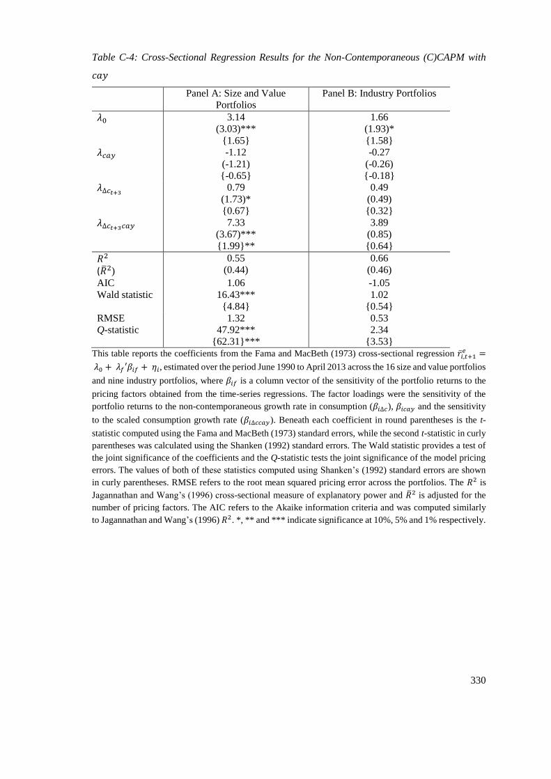
330

Table C-4: Cross-Sectional Regression Results for the Non-Contemporaneous (C)CAPM with

𝑐𝑎𝑦


Portfolios


𝜆0 3.14

(3.03)***

{1.65}

1.66

(1.93)*

{1.58}


(-1.21)

{-0.65}

-0.27

(-0.26)

{-0.18} 𝜆∆𝑐𝑡+3

0.79

(1.73)*

{0.67}

0.49

(0.49)

{0.32}

𝜆∆𝑐𝑡+3𝑐𝑎𝑦 7.33

(3.67)***

{1.99}**

3.89

(0.85)

{0.64}

𝑅2 (��2)

0.55

(0.44)

0.66

(0.46)

AIC 1.06 -1.05


{4.84}

1.02

{0.54}

RMSE 1.32 0.53


{62.31}***

2.34

{3.53}




pricing factors obtained from the time-series regressions. The factor loadings were the sensitivity of the

portfolio returns to the non-contemporaneous growth rate in consumption (𝛽𝑖∆𝑐), 𝛽𝑖𝑐𝑎𝑦 and the sensitivity

to the scaled consumption growth rate (𝛽𝑖∆𝑐𝑐𝑎𝑦). Beneath each coefficient in round parentheses is the t-

statistic computed using the Fama and MacBeth (1973) standard errors, while the second t-statistic in curly

parentheses was calculated using the Shanken (1992) standard errors. The Wald statistic provides a test of

the joint significance of the coefficients and the Q-statistic tests the joint significance of the model pricing

errors. The values of both of these statistics computed using Shanken’s (1992) standard errors are shown

in curly parentheses. RMSE refers to the root mean squared pricing error across the portfolios. The 𝑅2 is

Jagannathan and Wang’s (1996) cross-sectional measure of explanatory power and ��2 is adjusted for the

number of pricing factors. The AIC refers to the Akaike information criteria and was computed similarly

to Jagannathan and Wang’s (1996) 𝑅2. *, ** and *** indicate significance at 10%, 5% and 1% respectively.

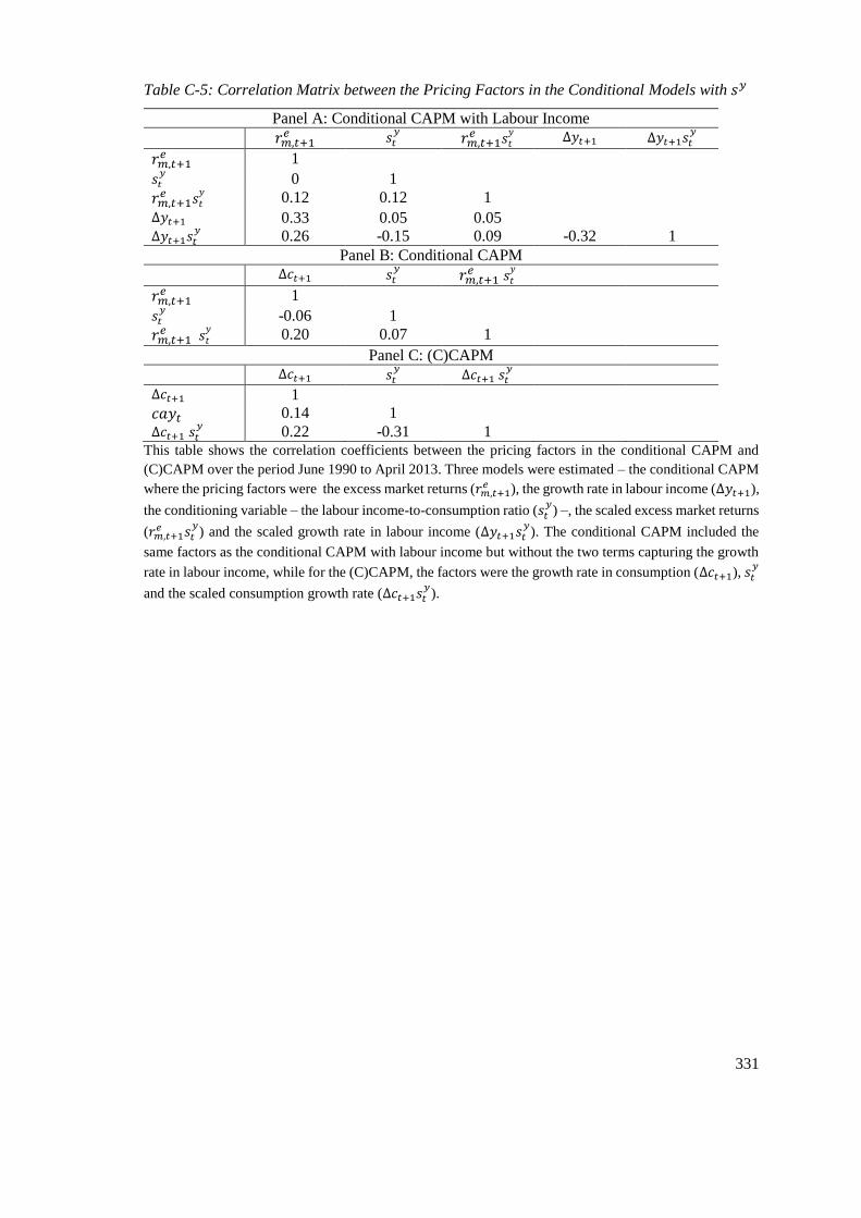
331

Table C-5: Correlation Matrix between the Pricing Factors in the Conditional Models with 𝑠𝑦

Panel A: Conditional CAPM with Labour Income

𝑟𝑚,𝑡+1𝑒 𝑠𝑡

𝑦 𝑟𝑚,𝑡+1

𝑒 𝑠𝑡𝑦 ∆𝑦𝑡+1 ∆𝑦𝑡+1𝑠𝑡

𝑦


𝑠𝑡𝑦

0 1


𝑦 0.12 0.12 1

∆𝑦𝑡+1 0.33 0.05 0.05 ∆𝑦𝑡+1𝑠𝑡

𝑦 0.26 -0.15 0.09 -0.32 1

Panel B: Conditional CAPM

∆𝑐𝑡+1 𝑠𝑡𝑦 𝑟𝑚,𝑡+1

𝑒 𝑠𝑡𝑦


𝑠𝑡𝑦

-0.06 1


𝑦 0.20 0.07 1

Panel C: (C)CAPM

∆𝑐𝑡+1 𝑠𝑡𝑦 ∆𝑐𝑡+1 𝑠𝑡

𝑦

∆𝑐𝑡+1 1

𝑐𝑎𝑦𝑡 0.14 1

∆𝑐𝑡+1 𝑠𝑡𝑦 0.22 -0.31 1

This table shows the correlation coefficients between the pricing factors in the conditional CAPM and

(C)CAPM over the period June 1990 to April 2013. Three models were estimated – the conditional CAPM

where the pricing factors were the excess market returns (𝑟𝑚,𝑡+1𝑒 ), the growth rate in labour income (∆𝑦𝑡+1),

the conditioning variable – the labour income-to-consumption ratio (𝑠𝑡𝑦

) –, the scaled excess market returns

(𝑟𝑚,𝑡+1𝑒 𝑠𝑡

𝑦) and the scaled growth rate in labour income (∆𝑦𝑡+1𝑠𝑡

𝑦). The conditional CAPM included the

same factors as the conditional CAPM with labour income but without the two terms capturing the growth

rate in labour income, while for the (C)CAPM, the factors were the growth rate in consumption (∆𝑐𝑡+1), 𝑠𝑡𝑦

and the scaled consumption growth rate (∆𝑐𝑡+1𝑠𝑡𝑦

).

332

Table C-6: Cross-Sectional Regression Results for the Non-Contemporaneous (C)CAPM with 𝑠𝑦


Portfolios


𝜆0 4.24

(4.03)***

{2.99}***

3.80

(3.00)***

{1.74}*

𝜆𝑠𝑦 -0.04

(-0.25)

{-0.19}

0.43

(1.71)*

{0.95}

𝜆∆𝑐𝑡+3 -0.61

(-0.81)

{-0.60}

-1.84

(-1.19)

{-0.65}

𝜆∆𝑐𝑡+3𝑠𝑦 -1.01

(-1.94)*

{-1.43}

0.51

(1.13)

{0.57}

𝑅2

(��2)

0.24

(0.05)

0.62

(0.39)

AIC 1.59 -0.92

Wald statistic 4.49

{2.46}

5.63

{1.65}

RMSE 1.67 0.42


{75.43}***

2.46

{0.29}




pricing factors obtained from the time-series regressions. The factor loadings were the sensitivity of the

portfolio returns to the growth rate in consumption (𝛽𝑖∆𝑐), the sensitivity to the labour income-to-

consumption ratio, 𝑠𝑡𝑦

, (𝛽𝑖𝑠𝑡𝑦) and the sensitivity to the scaled consumption growth rate (𝛽𝑖∆𝑐𝑠𝑡

𝑦). Beneath

each coefficient in round parentheses is the t-statistic computed using the Fama and MacBeth (1973)

standard errors, while the second t-statistic in curly parentheses was calculated using the Shanken (1992)

standard errors. The Wald statistic provides a test of the joint significance of the coefficients and the Q-

statistic tests the joint significance of the model pricing errors. The values of both of these statistics

computed using Shanken’s (1992) standard errors are shown in curly parentheses. RMSE refers to the root

mean squared pricing error across the portfolios. The 𝑅2 is Jagannathan and Wang’s (1996) cross-sectional

measure of explanatory power and ��2 is adjusted for the number of pricing factors. The AIC refers to the

Akaike information criteria and was computed similarly to Jagannathan and Wang’s (1996) 𝑅2.

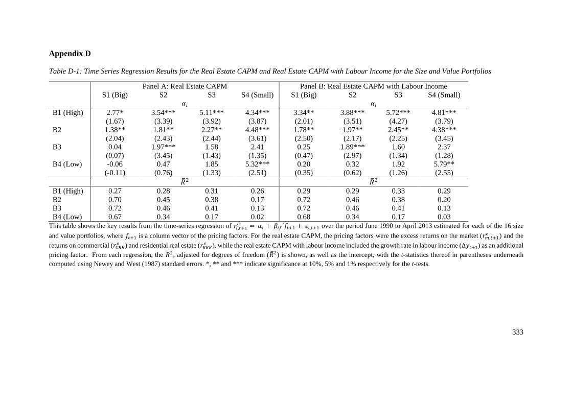
333

Appendix D

Table D-1: Time Series Regression Results for the Real Estate CAPM and Real Estate CAPM with Labour Income for the Size and Value Portfolios

Panel A: Real Estate CAPM Panel B: Real Estate CAPM with Labour Income S1 (Big) S2 S3 S4 (Small) S1 (Big) S2 S3 S4 (Small)

𝛼𝑖 𝛼𝑖

B1 (High) 2.77*

(1.67)

3.54***

(3.39)

5.11***

(3.92)

4.34***

(3.87)

3.34**

(2.01)

3.88***

(3.51)

5.72***

(4.27)

4.81***

(3.79)

B2 1.38**

(2.04)

1.81**

(2.43)

2.27**

(2.44)

4.48***

(3.61)

1.78**

(2.50)

1.97**

(2.17)

2.45**

(2.25)

4.38***

(3.45)

B3 0.04

(0.07)

1.97***

(3.45)

1.58

(1.43)

2.41

(1.35)

0.25

(0.47)

1.89***

(2.97)

1.60

(1.34)

2.37

(1.28)

B4 (Low) -0.06

(-0.11)

0.47

(0.76)

1.85

(1.33)

5.32***

(2.51)

0.20

(0.35)

0.32

(0.62)

1.92

(1.26)

5.79**

(2.55) ��2 ��2

B1 (High) 0.27 0.28 0.31 0.26 0.29 0.29 0.33 0.29

B2 0.70 0.45 0.38 0.17 0.72 0.46 0.38 0.20

B3 0.72 0.46 0.41 0.13 0.72 0.46 0.41 0.13

B4 (Low) 0.67 0.34 0.17 0.02 0.68 0.34 0.17 0.03

This table shows the key results from the time-series regression of 𝑟𝑖,𝑡+1𝑒 = 𝛼𝑖 + 𝛽𝑖𝑓′𝑓𝑡+1 + 휀𝑖,𝑡+1 over the period June 1990 to April 2013 estimated for each of the 16 size

and value portfolios, where 𝑓𝑡+1 is a column vector of the pricing factors. For the real estate CAPM, the pricing factors were the excess returns on the market (𝑟𝑚,𝑡+1𝑒 ) and the

returns on commercial (𝑟𝐶𝑅𝐸𝑒 ) and residential real estate (𝑟𝑅𝑅𝐸

𝑒 ), while the real estate CAPM with labour income included the growth rate in labour income (∆𝑦𝑡+1) as an additional

pricing factor. From each regression, the 𝑅2, adjusted for degrees of freedom (��2) is shown, as well as the intercept, with the t-statistics thereof in parentheses underneath

computed using Newey and West (1987) standard errors. *, ** and *** indicate significance at 10%, 5% and 1% respectively for the t-tests.

334

Table D-2: Time Series Regression Results for the Real Estate CAPM and Real Estate CAPM

with Labour Income on the Industry Portfolios

Real Estate CAPM Real Estate CAPM with Labour

Income


Basic Materials -0.09

(-0.08)

0.55 0.76

(0.68)

0.60

Consumer Goods 0.61

(0.94)

0.66 0.52

(0.79)

0.66


(1.53)

0.40 1.48

(0.95)

0.42

Financials 0.68

(1.07)

0.57 0.35

(0.51)

0.59

Health Care 2.17***

(5.24)

0.10 2.02

(1.31)

0.10

Industrials 0.57

(0.84)

0.52 0.62

(0.92)

0.52

Oil and Gas 1.07

(0.82)

0.20 1.95

(1.42)

0.26

Technology -0.22

(-0.11)

0.31 -0.73

(-0.36)

0.32


(0.94)

0.20 1.09

(0.68)

0.20

This table shows the key results from the time-series regression of 𝑟𝑖,𝑡+1𝑒 = 𝛼𝑖 + 𝛽𝑖𝑓′𝑓𝑡+1 + 휀𝑖,𝑡+1 over the

period June 1990 to April 2013 estimated for each of the nine industry portfolios, where 𝑓𝑡+1 is a column

vector of the pricing factors. For the real estate CAPM, the pricing factors were the excess returns on the

market (𝑟𝑚,𝑡+1𝑒 ) and the returns on commercial (𝑟𝐶𝑅𝐸

𝑒 ) and residential real estate (𝑟𝑅𝑅𝐸𝑒 ), while the real estate

CAPM with labour income included the growth rate in labour income (∆𝑦𝑡+1) as an additional pricing

factor. From each regression, the 𝑅2, adjusted for degrees of freedom (��2) is shown, as well as the intercept,

with the t-statistics thereof in parentheses underneath computed using Newey and West (1987) standard

errors. *, ** and *** indicate significance at 10%, 5% and 1% respectively for the t-tests.

335

Table D-3: Correlation Matrix between the Pricing Factors in the Collateral Housing Models

∆𝑛ℎ𝑡+1 𝛼𝑡 ∆𝑛ℎ𝑡+1𝛼𝑡 𝛥𝛼𝑡+1 𝛥𝛼𝑡+1𝛼𝑡

∆𝑛ℎ𝑡+1 1

𝛼𝑡 -0.14 1

∆𝑛ℎ𝑡+1𝛼𝑡 0.25 0.23 1

𝛥𝛼𝑡+1 0.48 -0.09 0.27 1

𝛥𝛼𝑡+1𝛼𝑡 0.25 -0.03 0.37 -0.15 1 This table shows the correlation coefficients between the pricing factors in the collateral housing models

of Piazzesi et al. (2003) over the period June 1990 to April 2013. Four models were estimated – the non-

housing consumption CAPM where the pricing factor was the non-housing consumption growth rate

(∆𝑛ℎ𝑡+1); the CH-CAPM where the pricing factors were ∆𝑛ℎ𝑡+1 and the change in the expenditure share

of non-housing consumption to total consumption (𝛥𝛼𝑡+1); the (C)CAPM where the factors included

∆𝑛ℎ𝑡+1, the conditioning variable, 𝛼𝑡, and the scaled non-housing consumption growth rate ∆𝑛ℎ𝑡+1𝛼𝑡;

while for the conditional CH-CAPM, the pricing factors included ∆𝑛ℎ𝑡+1, 𝛼𝑡, 𝛥𝛼𝑡+1, ∆𝑛ℎ𝑡+1𝛼𝑡 and the

scaled change in the expenditure share (𝛥𝛼𝑡+1𝛼𝑡, ).

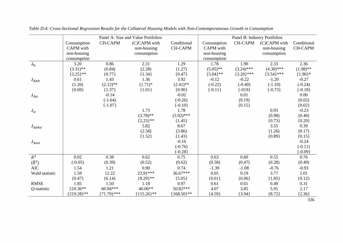
336

Table D-4: Cross-Sectional Regression Results for the Collateral Housing Models with Non-Contemporaneous Growth in Consumption


Consumption

CAPM with

non-housing

consumption


non-housing

consumption

Conditional

CH-CAPM

Consumption

CAPM with

non-housing

consumption


non-housing

consumption

Conditional

CH-CAPM

𝜆0 3.20

(3.31)**

{3.25}**

0.86

(0.84)

{0.77}

2.31

(2.28)

{1.34}

1.29

(1.27)

{0.47}

1.78

(5.05)**

{5.04}**

1.90

(3.24)***

{3.20}***

2.33

(4.30)***

{3.54}***

2.36

(1.98)**

{1.90}*

𝜆Δ𝑛ℎ 0.61

(1.26)

{0.69}

1.43

(2.12)**

{1.37}

1.36

(1.71)*

{1.01}

3.92

(2.41)**

{0.90}

-0.12

(-0.22)

{-0.11}

-0.22

(-0.40)

{-019}

-1.20

(-1.10)

{-0.73}

-0.27

(-0.24)

{-0.18}

𝜆Δ𝛼 -0.14

(-1.64)

{-1.07}

-0.02

(-0.26)

{-0.10}

0.01

(0.19)

{0.15}

0.00

(0.02)

{0.02} 𝜆𝛼 1.73

(3.78)**

{2.23}**

1.78

(3.92)***

{1.45}

0.93

(0.98)

{0.73}

-0.23

(0.40)

{0.29}

𝜆Δnh𝛼 5.82

(2.58)

{1.52}

8.67

(3.86)

{1.43}

3.55

(1.26)

{0.89}

0.39

(0.17)

{0.15}

𝜆Δ𝛼𝛼 -0.16

(-0.76)

{-0.28}

-0.24

(-0.11)

{-0.09}

𝑅2 (��2)

0.02

(-0.05)

0.38

(0.39)

0.62

(0.52)

0.75

(0.62)

0.63

(0.58)

0.60

(0.47)

0.55

(0.28)

0.76

(0.49)

AIC 1.54 1.21 0.90 0.74 -1.39 -1.08 -0.76 -0.93

Wald statistic 1.59

{0.47}

12.22

{6.14}

23.91***

{8.29}**

36.67***

{5.05}

0.05

{0.01}

0.19

{0.06}

3.77

{1.85}

1.01

{0.12}

RMSE 1.85 1.50 1.18 0.97 0.61 0.61 0.49 0.31

Q-statistic 210.36**

{219.28}** 60.94***

{71.79}*** 40.06**

{115.26}**

50.82***

{168.50}** 4.07

{4.59} 3.85

{3.94} 5.91

{8.72}

2.17

{2.36}

337



obtained from the time-series regressions. For the non-housing consumption CAPM, the factor loading was the sensitivity to the growth rate in non-housing consumption

(𝛽𝑖∆𝑛ℎ), while for the CH-CAPM, the factor loadings included 𝛽𝑖∆𝑛ℎ and the sensitivity to changes in the expenditure share of non-housing consumption to total consumption

(𝛽𝑖∆𝛼). For the (C)CAPM, the factor loadings were 𝛽𝑖∆𝑛ℎ, the sensitivity to the conditioning variable, 𝛽𝑖𝛼 and the sensitivity to the scaled non-housing consumption growth rate

(𝛽𝑖∆𝑛ℎ𝛼), while for the conditional CH-CAPM, the factor loadings included 𝛽𝑖∆𝑛ℎ, 𝛽𝑖𝛼 , 𝛽𝑖∆𝛼, 𝛽𝑖∆𝑛ℎ𝛼 and the sensitivity to the scaled change in the expenditure share (𝛽𝑖∆𝛼𝛼). All

consumption growth rates were measured over three-quarters. Beneath each coefficient in round parentheses is the t-statistic computed using the Fama and MacBeth (1973)

standard errors, while the second t-statistic in curly parentheses was calculated using the Shanken (1992) standard errors. The Wald statistic provides a test of the joint

significance of the coefficients and the Q-statistic tests the joint significance of the model pricing errors. The values of both of these statistics computed using Shanken’s (1992)

standard errors are shown in curly parentheses. RMSE refers to the root mean squared pricing error across the portfolios. The 𝑅2 is Jagannathan and Wang’s (1996) cross-

sectional measure of explanatory power and ��2 is adjusted for the number of pricing factors. The AIC computed follows the approach proposed by Jagannathan and Wang

(1996). *, ** and *** indicate significance at 10%, 5% and 1% respectively for the various tests.

338

Table D-5: Correlation Matrix between the Pricing Factors in the Collateral CAPM

∆𝑛ℎ𝑡+1 𝑚��𝑡 ∆𝑛ℎ𝑡+1𝑚��𝑡 𝛥𝛼𝑡+1 𝛥𝛼𝑡+1𝑚��𝑡

∆𝑛ℎ𝑡+1 1

𝑚��𝑡 -0.07 1

∆𝑛ℎ𝑡+1𝑚��𝑡 0.13 0.19 1

𝛥𝛼𝑡+1 0.46 -0.11 0.05 1

𝛥𝛼𝑡+1𝑚��𝑡 0.08 0.38 0.38 0.11 1

This table shows the correlation coefficients between the pricing factors in the collateral CAPM of Lustig and van

Nieuwerburgh (2005) over the period June 1990 to April 2013. Four models were estimated – the non-housing

consumption CAPM where the pricing factor was the non-housing consumption growth rate (∆𝑛ℎ𝑡+1); the CH-

CAPM where the pricing factors were ∆𝑛ℎ𝑡+1 and the change in the expenditure share

of non-housing consumption to total consumption (𝛥𝛼𝑡+1); the (C)CAPM where the factors included ∆𝑛ℎ𝑡+1, the

conditioning variable, 𝛼𝑡, and the scaled non-housing consumption growth rate ∆𝑛ℎ𝑡+1𝛼𝑡; while for the

conditional CH-CAPM, the pricing factors included ∆𝑛ℎ𝑡+1, 𝛼𝑡, 𝛥𝛼𝑡+1, ∆𝑛ℎ𝑡+1𝛼𝑡 and the scaled change in the

expenditure share (𝛥𝛼𝑡+1𝛼𝑡).

339

Table D-6: Cross-Sectional Results for the Non-Contemporaneous Collateral CAPM


Separable

preferences

Non-separable

preferences

Separable

preferences

Non-separable

preferences

𝜆0 0.70

(0.71)

{0.45}

2.31

(2.06)**

{0.88}

1.67

(3.01)***

{2.96}***

1.94

(2.19)**

{2.15}**

𝜆∆𝑛ℎ𝑡+3 0.97

(1.72)**

{0.90}

1.77

(2.35)**

{1.00}

-0.34

(-0.52)

{-0.28}

0.11

(0.17)

{0.09}

𝜆𝑚𝑦 0.14

(3.70)***

{2.30}**

0.08

(1.80)*

{0.77}

0.01

(0.15)

{0.13}

-0.02

(-0.25)

{-0.21}

𝜆∆𝑛ℎ𝑚𝑦 0.39

(3.09)***

{1.94}*

0.55

(4.35)***

{1.85}*

0.06

(0.37)

{0.28}

0.07

(0.34)

{0.27}

𝜆∆𝛼 -0.05

(-0.84)

{-0.35}

-0.05

(-0.34)

{-0.29}

𝜆∆𝛼𝑚𝑦 -0.04

(-1.51)

{-1.07}

-0.02

(-1.42)

{-0.01}

𝑅2

(��2)

0.58

(0.48)

0.65

(0.48)

0.65

(0.45)

0.83

(0.58)

AIC 0.94 1.01 -1.02 -1.29


{9.31}**

34.68***

{6.71}

1.78

{0.73}

4.24

{1.74}

RMSE 1.05 1.10 0.59 0.21


{89.97}***

36.72***

{126.36}***

4.31

{4.46}

1.46

{1.50} This table reports the coefficients from the Fama and MacBeth (1973) cross-sectional regression ��𝑖,𝑡+1

𝑒 = 𝜆0 +

𝜆𝑓′𝛽𝑖𝑓 + 𝜂𝑖, estimated over the period June 1990 to April 2013 across the 16 size and value portfolios and nine

industry portfolios, where 𝛽𝑖𝑓 is a column vector of the sensitivity of the portfolio returns to the pricing factors

(factor loadings) obtained from the time-series regressions. For the collateral CAPM with separable preferences,

the factor loading was the sensitivity of the portfolio returns to the growth rate in non-contemporaneous non-

housing consumption (𝛽𝑖∆𝑛ℎ) (measured over three quarters) the sensitivity to the housing scarcity ratio (𝛽𝑖𝑚��)

and the sensitivity to the scaled growth rate in non-contemporaneous non-housing consumption (𝛽𝑖∆𝑛ℎ𝑚��). For

the collateral CAPM with non-separable preferences two additional factor loadings were included - the sensitivity

to the change in the expenditure share on non-housing consumption relative to total consumption (𝛽𝑖∆𝛼) and the

scaled expenditure share (𝛽𝑖∆𝛼𝑚��). Beneath each coefficient in round parentheses is the t-statistic computed using

the Fama and MacBeth (1973) standard errors, while the second t-statistic in curly parentheses was calculated

using the Shanken (1992) standard errors. The Wald statistic provides a test of the joint significance of the

coefficients and the Q-statistic tests the joint significance of the model pricing errors. The values of both of these

statistics computed using Shanken’s (1992) standard errors are shown in curly parentheses. RMSE refers to the

root mean squared pricing error across the portfolios. The 𝑅2 is Jagannathan and Wang’s (1996) cross-sectional

measure of explanatory power and ��2 is adjusted for the number of pricing factors. The AIC refers to the Akaike

information criteria and was computed similarly to Jagannathan and Wang’s (1996) 𝑅2. *, ** and *** indicate

significance at 10%, 5% and 1% respectively for the various tests.

340

Table D-7: Cross-sectional Regression Results for the Durable CAPM with ∆𝑑



Durable CAPM


Durable CAPM

𝜆0 7.30

(4.61)***

{3.41}***

5.74

(3.68)***

{2.72}***

3.46

(3.13)***

{2.93}***

3.09

(2.13)**

{2.06}** 𝜆𝑚 -6.50

(-3.10)***

{-2.22}***

-4.63

(-2.23)**

{-1.67}*

-2.31

(-0.93)

{-0.55}

-1.96

(-0.79)

{-0.48} 𝜆∆𝑐𝑡+1

0.65

(1.68)*

{0.98}

-0.04

(-0.10)

{-0.06}

𝜆Δ𝑑 -0.23

(-0.38)

{-0.28}

0.34

(0.68)

{0.44}

𝜆Δ𝑐𝑡+3 0.11

(0.17)

{0.12}

0.19

(0.37)

{0.18} 𝜆Δ𝑑𝑡+3

1.56

(2.24)**

{1.68}*

0.31

(0.33)

{0.21}

𝑅2 (��2)

0.39

(0.24) 0.58

(0.47) 0.78

(0.65) 0.63

(0.41)

AIC 1.27 1.15 -1.14 -0.85 Wald statistic 10.77**

{5.84} 10.02**

{6.80}*

1.33

{0.50} 0.87

{0.30} RMSE 1.42 5.44 0.42 0.45


{72.15}*** 38.25***

{64.85}*** 3.25

{3.71} 4.10

{4.41} This table reports the coefficients from the Fama and MacBeth (1973) cross-sectional regression ��𝑖,𝑡+1

𝑒 = 𝜆0 +

𝜆𝑓′𝛽𝑖𝑓 + 𝜂𝑖, estimated over the period June 1990 to April 2013 across the 16 size and value portfolios and nine

industry portfolios, where 𝛽𝑖𝑓 is a column vector of the sensitivity of the portfolio returns to the pricing factors

(factor loadings) obtained from the time-series regressions. For the durable CAPM, the factor loadings were the

sensitivity to the growth rate in non-durable consumption (𝛽𝑖∆𝑐), durable consumption (𝛽𝑖∆𝑑) (where growth in

durable goods only included durable goods and not semi-durable goods, denoted ∆𝑑) and the excess real market

returns (𝛽𝑖𝑚). For the non-contemporaneous specification, the factor loadings are identical but are measured

relative to the non-contemporaneous growth rates (measured over three quarters) on durable and non-durable

consumption respectively. Beneath each coefficient in round parentheses is the t-statistic computed using the

Fama and MacBeth (1973) standard errors, while the second t-statistic in curly parentheses was calculated using

the Shanken (1992) standard errors. The Wald statistic provides a test of the joint significance of the coefficients

and the Q-statistic tests the joint significance of the model pricing errors. The values of both of these statistics

computed using Shanken’s (1992) standard errors are shown in curly parentheses. RMSE refers to the root mean

squared pricing error across the portfolios. The 𝑅2 is Jagannathan and Wang’s (1996) cross-sectional measure of

explanatory power and ��2 is adjusted for the number of pricing factors. The AIC refers to the Akaike information

criteria and was computed similarly to Jagannathan and Wang’s (1996) 𝑅2. *, ** and *** indicate significance at

10%, 5% and 1% respectively for the various tests.

341

ETHICAL CLEARANCE

explaining the cross-section of share returns in …

Documents