Experiments in Robotic Boat Localization

Amit Dhariwal and Gaurav S. SukhatmeDepartment of Computer Science, University of Southern California,

Los Angeles, California, USA{dhariwal, gaurav}@usc.edu

Abstract—We are motivated by the prospect of automatingmicrobial observing systems. To this end we have designedand built a robotic boat as part of a sensor network formonitoring aquatic environments. In this paper, we describea dynamic model of the boat, an algorithm for estimatingits location by integrating various sensor inputs, a controllerfor waypoint following and extensive field experiments (over10 km aggregate) to validate each of these. We test thelocalization accuracy in different sensing regimes as a preludeto accommodating sensing failures.

I. INTRODUCTION

The microbiology of aquatic environments is of scientificinterest [1]. Its characterization affects our understandingof aquatic food webs, and the impact of urbanization andpollution. It also ultimately plays a role in setting publicpolicy (e.g. regulations on dumping), and other decisionmaking (e.g. when is a beach closure necessary because thewater is contaminated?).Aquatic environmental monitoring has traditionally been

done by a human operator performing the sampling man-ually. This process is inherently slow, tedious, and expen-sive. To alleviate this, our work is aimed at developinga sensor network to monitor aquatic environments. Ournetwork is composed of static, anchored buoys, and arobotic boat (henceforth ’the boat’) all of which commu-nicate with each other. Simply put, the static nodes pro-vide excellent temporal sampling resolution but a limitedspatial resolution. The boat is able to traverse the watersurface providing high spatial resolution of the data col-lected but limited temporal resolution. The overall systemNAMOS (Networked Aquatic Microbial Observing System)is described in [2], [3] and is extensively documentedat http://robotics.usc.edu/namos. The projectwebsite also contains the biological data collected over thecourse of several weeks of field experiments during which theboat traveled in excess of 10 km aggregate. The focus of thispaper is on the development of a dynamic model of the boat,an algorithm for estimating its location by integrating sensorinputs, a controller for waypoint following and extensive fieldexperiments to validate each of these.The interplay of ocean currents, waves and wind and

their combined effect on watercraft is difficult to model andcompensate. Even a seemingly simple action, like stationkeeping for a boat, can be very difficult. Navigation in suchan environment is equally difficult. Imagine driving a bicycleon a suspended rope bridge, with the bridge swaying due

to wind as well as moving due to your changing position.Inherent in their nature, both waves and wind vary over timeboth in speed and direction in a complex manner. This makesit difficult to compensate for them without having accurateand reliable sensors on board the boat. Marine vessel controlis a extensively deliberated problem [4]–[6]. Most researchin this area has been driven by the requirements of marineapplications including off-shore drilling, fisheries and trans-portation of goods and people. Work on off shore drillingplatforms and ships require sea keeping or maintaining po-sition in the presence of wind and water disturbances. Mostmarine systems use underwater propulsion. The requirementsof application warrant the use of an air propeller so as tominimize the disturbance to surface water (which we aretrying to sample). Thus our prototype boat is the air-boatshown in Figure 1.Surface aquatic applications like the one considered here,

require only three degrees of freedom to be considered.These are: the motion along the longitudinal axis (surge),translational axis (sway) and rotation along the z axis (yawor heading) as shown in Figure 4. It is sufficient to accuratelyand reliably estimate the position (latitude and longitude) andorientation (heading or yaw) of the boat to keep it on trackand reach its target locations.Mobile robot localization is a widely studied problem.

However a majority of the work has been focused onland-based robots [7]–[11] and more recently on aerialvehicles [12], [13] and underwater systems [14], [15]. Forwatercraft, most prior work is for large marine vessels [4]–[6]which mostly deals with dynamic positioning (sea keeping)and steering or maneuvering i.e., ship motion without waveaction.Contributions:We describe a dynamic model of the boat,

an algorithm for estimating its location by integrating sensorinputs, a controller for waypoint following and extensivefield experiments (over 10 km aggregate) to validate eachof these. Specifically, we test the localization accuracy indifferent sensing regimes as a prelude to accommodatingsensing failures.

II. SYSTEM DESCRIPTIONThe boat used for testing is a modified radio controlled

airboat designed to perform surface sampling (chlorophylland temperature) at locations of interest. An airboat was cho-sen as it provides minimal disturbance to the water surfacewhile moving by reducing surface water mixing. We chose a

Fig. 1. Robotic Boat

split hull boat design since two pontoons make for a stableconfiguration. The boat is equipped with a commercial off-the-shelf GPS (Garmin 16A) and compass (Honeywell HMR3000) (Figure 2). Both the GPS and compass output NMEAstrings at configurable data rates making them ideal for usein our application. We use wind direction and speed sensorsfrom Texas Electronics. See Table I for details on typicalsensor characteristics. An Intel X-Scale Stargate processor(PXA 255, 400MHz), is the main processor on the boat. Itwas selected because of its relatively small form factor, goodperformance and low power consumption characteristics. Itssmall size makes it easy to fit it inside the relatively smallspace available on the boat. It also provides an 802.11b-based wireless link which is used by the boat to transmit andreceive data in real time. The navigation hardware on the boatconsists of an air propeller and a custom-built rudder whichare controlled by a basic stamp module (Parallax BS2sx).

Fig. 2. Sensors. (a) GPS, (b) Compass, (c) Wind direction and (d) Windspeed

The boat monitors two aspects of its environment - thetemperature (via a thermistor) and the relative chlorophyll-A concentration (via a CYCLOPS-7 submersible fluorometerfrom Turner Designs Inc.). The output from these is digitizedonboard via a 16 bit ADC. These two sensors are suspended

TABLE ITYPICAL SENSOR CHARACTERISTICS. FROM INSTRUMENT MANUALS

PROVIDED BY MANUFACTURER

Method Sensor Obs. Accuracy UpdateRate

Positioning Garmin x,y < 15m (Raw) 1Hz16A GPS 3− 5m

(with DGPSCorrection)

Heading Honeywell(Compass) HMR 3000 ψ 0.5◦ 13.75Hz

Texas ElectronicsWind speed TV-4 Sensor vw ±0.89m/s 1HzWind direction TD-4 Sensor γw ±3◦ 1Hz

into the water from the side of the boat (Figure 3). The boatalso has a custom built 6 port water sampling system whichcan collect water samples for lab analysis at specified GPSlocations. The boat is powered using rechargeable NiMHbatteries and can run for 4-6 hours without recharging.

Fig. 3. Environmental sensors on the boat. (a) Water sampler, and (b)fluorometer and thermistor

III. SYSTEM MODELFor aquatic applications involving boats and ships, only

three degrees of freedom are practically important [5], [16].These lie in the plane parallel to the surface of the water,namely surge, sway and yaw (Figure 4). It is based uponthe fact that the boat only moves in a plane parallel to thesurface of water (will not go above or below water (z-axis))and turn only along the z axis (without tilting or tippingover). For a relatively stable surface craft, this turns out tobe a safe assumption and helps simplify the boat model.It is also common to separate the analysis into two parts,namely the low frequency model (in 3D, described above)and a wave-frequency model which is generally added as anoutput disturbance.While there are several ways to represent the coordinate

system and associated nomenclature, we adopt the widely

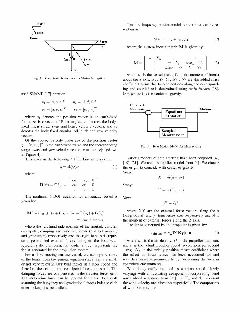
Fig. 4. Coordinate System used in Marine Navigation

used SNAME [17] notation:

η1 = [x, y, z]T η2 = [φ, θ, ψ]

T

ν1 = [u, v, w]T ν2 = [p, q, r]

T

where η1 denotes the position vector in an earth-fixedframe, η2 is a vector of Euler angles, ν1 denotes the body-fixed linear surge, sway and heave velocity vectors, and ν2denotes the body fixed angular roll, pitch and yaw velocityvectors.Of the above, we only make use of the position vector

η = [x, y, ψ]T in the earth-fixed frame and the correspondingsurge, sway and yaw velocity vectors ν = [u, v, r]T (shownin Figure 4).This gives us the following 3 DOF kinematic system:

η = R(ψ)ν (1)

where

R(ψ) = CTz,ψ =

⎡⎣ cψ −sψ 0sψ cψ 00 0 1

⎤⎦The nonlinear 6 DOF equation for an aquatic vessel is

given by:

Mν +CRB(ν)ν +CA(νr)νr +D(νr) +G(η)

= τenv + τthrust

where the left hand side consists of the inertial, coriolis,centripetal, damping and restoring forces (due to buoyancyand gravitation) respectively and the right hand side repre-sents generalized external forces acting on the boat, τenvrepresents the environmental loads, τthrust represents thethrust generated by the propulsion system.For a slow moving surface vessel, we can ignore some

of the terms from the general equation since they are smallor not very relevant. Our boat moves at a slow speed andtherefore the coriolis and centripetal forces are small. Thedamping forces are compensated in the thruster force term.The restoration force can be ignored for the surface craftassuming the buoyancy and gravitational forces balance eachother to keep the boat afloat.

The low frequency motion model for the boat can be re-written as:

Mν = τenv + τthrust (2)

where the system inertia matrix M is given by:

M =

⎡⎣ m−Xu 0 00 m− Yv mxG − Yr0 mxG − Yr Iz −Nr

⎤⎦ (3)

where m is the vessel mass, Iz is the moment of inertiaabout the z axis. Xu, Yv , Yr, Nv , Nr are the added masscoefficient terms due to accelerations along the correspond-ing and coupled axis determined using strip theory [18].(xG, yG, zG) is the center of gravity.

Fig. 5. Boat Motion Model for Maneuvering

Various models of ship steering have been proposed [4],[19]–[21]. We use a simplified model from [4]. We choosethe origin to coincide with center of gravity.Surge:

X =m(u− vr)

Sway:Y = m(v + ur)

Yaw:N = Iz r

where X,Y are the external force vectors along the x(longitudinal) and y (transverse) axes respectively and N isthe moment of external forces along the Z axis.The thrust generated by the propeller is given by:

τthrust = ρwD4KT|n|n (4)

where ρw is the air density, D is the propeller diameter,and n is the actual propeller speed (revolutions per second- rps). KT is the strictly positive thrust coefficient wherethe effect of thrust losses has been accounted for andwas determined experimentally by performing the tests incontrolled environments.Wind is generally modeled as a mean speed (slowly

varying) with a fluctuating component incorporating windgusts added as a noise term [22]. Let Vw and βw representthe wind velocity and direction respectively. The componentsof wind velocity are:

uw = Vw cos(βw − ψ) vw = Vw sin(βw − ψ) (5)

and the relative wind velocity vector is given by:

νrw = [u− uw, v − vw, r]T

The total relative wind velocity is:

Urw =p(u− uw)2 + (v − vw)2 (6)

The relative wind angle can be found by:

γw = atan2(−(v − vw),−(u− uw)) (7)

The wind load vector is then given by:

τwind = 0.5ρa

⎡⎣ AxCwx(γw)|Urw|Urw

AyCwy(γw)|Urw|Urw

AyLCwψ(γw)|Urw|Urw

⎤⎦ (8)

Here ρa is the density of air, L is the overall length of theboat, Ax and Ay are the lateral and longitudinal areas of thenon-submerged part of the boat projected on the xz-plane andyz-plane respectively, Cwx(γw), Cwy(γw) andCwψ(γw) arethe non-dimensional wind coefficients in surge, sway andyaw respectively. These are determined experimentally.

IV. LOCALIZATIONWe implement an extended Kalman filter to which sensor

inputs are provided as and when they arrive. The global po-sitioning system (GPS) provides position measurements, thecompass provides the heading (orientation) measurementsand the wind sensors provide the measurements related towind speed and direction. Each of the sensors has its ownupdate rate and error characteristics. In the absence of anysensor measurements arriving, the filter proceeds by deadreckoning using the dynamic model of the boat. If some ofthe sensors are not available, the filter localizes the boat usingthe ones that are available.The state vector consists of the position [x, y, ψ] and ve-

locity [u, v, r] vectors in the 3 DOF discussed in Section III.The system model is:

xk = f(xk−1, uk) + τwk;wk ∼ N(0, Qk)

The measurement model is:

zk = h(xk) + v(k); vk ∼ N(0,Rk)

We start from a known fixed location and provide itsinformation to the filter:

x0 = x0; P0 = P0

The filter operates in two phases. During the first phase(propagation phase), we propagate the state estimate anderror covariance using the following equations:

x−k = f(xk−1, uk)

P−k = φkPk−1φTk + τkQk−1τTk

During the second phase (update phase), whenever wereceive a measurement update, the gain matrix, state esti-mate and error covariance are updated using the followingequations:

Kk = P−k HTk [HkP

−k HT

k +Rk]−1

xk = x−k +Kk[zk − h(x−k )]

Pk = [I −KkHk]P−k

whereφk = ∂f(.)/∂xk|xk=xk

Hk = ∂h(.)/∂xk|xk=xkThe filter was implemented offline and its performance

was analyzed using data gathered from real boat experiments.These are described in Section VI.

V. CONTROL

In field experiments the boat can either be used in manualmode where the operator can specify the speed and headingof the boat via a joystick or in autonomous (waypointfollowing) mode where the operator uploads a sequenceof GPS locations designating the path to be followed bythe boat. Our waypoint following control is the commonlyused follow − the − carrot/goal method. The navigationalgorithm on the boat uses the current location estimate fromthe localization process and computes the distance to the nextwaypoint and the desired heading and generates the controlcommands for the boat (rudder angle and propeller speed)so as to minimize the heading and distance errors using PIDcontrol.The PI control equation for propeller speed control is

shown in Equation 9, where vcmd is the command sent tothe propeller control servo on the boat, vcur is the currentvelocity, vdes is the desired velocity, Kp is the proportionalgain and Ki is the integral gain. The gain terms weredetermined and tuned empirically based on experimentaldata.

vcmd = Kp(vdes − vcur) +Ki

Z(vdes − vcur)dt (9)

The PID control equation for rudder angle control is shownin Equation 10, where ψcmd is the command sent to therudder control servo on the boat, ψdes is the desired heading,ψcur is the current heading, Kphead is the proportional gain,Kdhead is the derivative gain and Kihead is the integral gain.

ψcmd = Kphead(ψdes − ψcur) +Kdhead(ψdes −−ψcur) +Kihead

Z(ψdes − ψcur)dt (10)

VI. EXPERIMENTS

A. Localization Experiments1) Setup and Data Collection: The data for the experi-

ments was gathered by performing several runs spanning aset of target points with the robotic boat. A specified pathwas chosen for the boat and visual markers were placed atlocations along this path. The exact location of these markerswas surveyed using differential GPS to provide ground truthinformation and this was used for comparing the results weobtained. We did not use the raw GPS data for comparisonof our results as it had large errors (between 7.5m and 11m).The boat was made to move along the path under human

guidance while the computer on the boat logged sensormeasurements from the GPS, compass and also the controlinputs sent to the motor controllers for the propeller andrudder. All the gathered data was time-stamped for offlineanalysis.Due to the limited payload capacity of the boat, we

could not mount the wind sensors on the boat. We madethe assumption that wind conditions (direction and speed)in a small open region on the surface of the lake arehomogeneous. This simplified the data gathering since itallowed us to gather wind direction and speed data by placinga weather station buoy along the actual path of the boat(rather than on the boat itself). We validated our assumptionof homogeneity by comparing the wind data reported by theweather buoy at points close to the start and end of the pathtaken by the boat. The clock on the boat and weather stationwere synchronized at the start of the experiment.2) Data Processing: Typical position accuracy achievable

by Garmin 16A GPS is less than 15m with a 95% confidencelevel (See Table I). Depending on the location of the exper-iment, we obtained accuracies between 7.5m and 11m. Theneed for better localization warrants us to use an extendedKalman filter.We use the model we developed in Section III. The

measurements from the GPS, compass and wind sensorswere made available to the extended Kalman filter at thesame rate and in the same order in which they were gatheredand were used in the update phase of the filter.The measurements from all the sensors do not arrive

simultaneously. They are processed in the order of arrival. Tohandle the problem of missing sensor measurements duringthe update phase, the corresponding columns in theH matrixare set to zero for the missing measurements.The GPS measurements provide the position of the boat

(latitude and longitude) in the earth-fixed frame which areconverted to northing’s and easting’s and provided to thefilter to update the estimate of the position of the boat (x, y).The compass measurements provide the heading of the

boat relative to the Earth’s geographic north. These mea-surements are provided to the filter to update the estimate ofthe orientation of the boat (ψ).The wind direction and speed measurements are provided

to the filter to update its estimate of the surge and swayvelocities (u, v).

TABLE IIFILTER INPUTS VS. ACCURACY (ECHO PARK)

Control Measurement Error Error ErrorInputs Inputs @40m @100m @160mYes None 28.14m 69.52m 117.57mYes Compass 7.98m 13.68m 19.63mYes Compass 4.23m 4.39m 6.31m

WindYes Compass 1.67m 1.41m 2.80m

GPS

z1 = xgps + v1 (surge-position)z2 = ygps + v2 (sway-position)z3 = ψcompass + v3 (yaw-angle)z4 = Vw + v4 (wind-speed)z5 = βw + v5 (wind-direction)where the measurement noise vi (i=1..5) is modeled as

zero-mean Gaussian white noise.We did not have measurements available to update the

velocity vector (u, v, r). These were in turn determined basedon the control inputs that were provided to the boat. We de-termined the conversion parameters for different commandedinputs into equivalent thruster force and conversion efficiencyparameters needed to determine the boat speed using theStraight-Line Test [5]. We also determined the turn ratecharacteristic and its coupling to the boat speed and rudderangle by carrying out these tests in still water.3) Results: We had two goals in mind while performing

these tests. We wanted to determine the performance of thefilter in the presence of selected sensors being available.To analyze this, the same measurement set was used butdifferent sensor measurement combinations were provided tothe filter. The combinations we tried and the correspondingresults for our two field sites are summarized in Tables II, III.The results presented in these tables are average valuesfrom 10 runs each over the same path. The data obtainedfrom differential GPS was used as ground truth for theseexperiments. In the table an average error of 1.67m at 40mfrom the start location using compass and GPS sensor asinput means that the location estimate from the extendedKalman filter was off by about 1.67m from the DGPSreported location (available ground truth). Figures 6, 7 showvisualizations depicting the predicted trajectory by the stateestimator in the presence of control inputs and differentsensor measurements.Our results indicate that a very accurate dynamic system

model is not required to perform good localization giventhe availability of a few sensors. Availability of a relativelysimple sensor like a compass which can provide headingmeasurements can greatly help in providing good localiza-tion. The availability of more sensor measurements of variouskinds (wind measurements, GPS etc.) helps improve thelocalization accuracy significantly. The results indicate thatin the absence of any measurement data, we need a veryeffective model of the boat to be able to localize it.

0 5 10 15 20 25 30 35 400

20

40

60

80

100

120

140

160

180

Easting (in m.)

Nor

thin

g (in

m.)

Effect of availability of measurements for State Estimation

No measurementsw/ Compassw/ Compass & Windw/ Compass & GPSStartEnd

Fig. 6. Result of localization on Echo Park data

0 2 4 6 8 10 12 14 16 18 200

5

10

15

20

25

30

35

40

Easting (in m.)

Nor

thin

g (in

m.)

Effect of availability of measurements for State Estimation

No measurementsw/ Compassw/ Compass & GPSStartEnd

Fig. 7. Result of localization on James Reserve data

B. Autonomous Navigation ExperimentsWe performed fifteen field tests with the boat to evaluate

its navigation performance. Our experiments were performedat Lake Fulmor, James Reserve, CA and Echo Park Lake inLos Angeles, CA.The boat was provided with a set of waypoints to be

traversed in the given order. A GPS and compass wereavailable on the boat to provide position and heading mea-surements. Wind measurements were not available duringthese experiments. The algorithm running on the boat usedthe measurements provided by the GPS and compass tocompute the control commands for the propeller and therudder.Figures 8, 9 show results from our autonomous runs with

the boat. The scale along x-axis for Figure 9 has beenscaled to give the reader a better feel for typical accuraciesachievable in the field by the GPS. The results indicatethat the boat follows the specified path (in terms of GPSway-points) closely and reaches the specified target locationswithin the specified acceptable range. Typical GPS accuracyachieved during these runs was between 7.5m and 11m (Notethat the errors are similar irrespective of the direction oftravel of the boat, i.e., going between north and south vs.

TABLE IIIFILTER INPUTS VS. ACCURACY (JAMES RESERVE)

Control Measurement Error Error ErrorInputs Inputs @35m @55m @93mYes None 33.76m 43.62m 46.88mYes Compass 9.64m 16.32m 18.07mYes Compass 7.63m 12.34m 14.32m

WindYes Compass 2.07m 2.19m 2.11m

GPS

east and west).The results demonstrate the very high dependence on

position measurements from GPS. This can be observed bycomparing the results presented in Figures 8, 9. Better GPSmeasurements were available at the Echo Park site comparedto the James Reserve site.

0 50 100 150 200 250 3000

50

100

150

200

250

300

Autonomous Navigation Results(James Reserve)

Easting (in m.)

Nor

thin

g (in

m.)

Specified way−point PathActual Path FollowedStart

Fig. 8. Result of autonomous navigation at James Reserve, CA

VII. CONCLUSIONS AND FUTURE WORKWe described a dynamic model of a robotic boat, an

algorithm for estimating its location by integrating sensorinputs, a controller for waypoint following and extensivefield experiments (over 10 km aggregate) to validate each ofthese. We tested the localization accuracy in different sensingregimes as a prelude to accommodating sensing failures.We are in the process of refining our boat model, as well as

implementing a framework for fault detection and recoveryas a prelude to using the boat as part of a measurementcampaign in the field.

VIII. ACKNOWLEDGEMENTSThe authors thank David Caron, Arvind Pereira, Steffi

Moorthi, Carl Oberg, and Beth Stauffer for their commentsand help with the experiments. This work is supported bythe National Science Foundation under grant CCF-0120778.

REFERENCES[1] D. A. Caron, “Marine microbial ecology in a molecular world: what

does the future hold?” Scientia Marina, no. 69, pp. 97–110 Suppl. 1,2005.

0 5 10 15 20 25 30 35 40 45 500

50

100

150

200

250

300

Easting (in m.)

Nor

thin

g (in

m.)

Autonomous Navigation Results (Echo Park)Specified way−point PathActual Path FollowedStart

Fig. 9. Result of autonomous navigation at Echo Park

[2] A. Dhariwal, B. Zhang, B. Stauffer, C. Oberg, G. S. Sukhatme,D. A. Caron, and A. A. Requicha, “Networked aquatic microbialobserving system,” in IEEE International Conference on Robotics andAutomation. Orlando, FL: IEEE, May 2006, pp. 4285–4287.

[3] G. S. Sukhatme, A. Dhariwal, B. Zhang, C. Oberg, B. Stauffer, andD. A. Caron, “The design and development of a wireless roboticnetworked aquatic microbial observing system,” Environmental En-gineering Science, 2006.

[4] T. Fossen,Marine Control Systems: Guidance, Navigation and Controlof Ships, Rigs and Underwater Vehicles. Marine Cybernetics AS,Trondheim. ISBN 82-92356-00-2, 2002, 1st. Ed., 3rd. Printing, 586pages.

[5] T. Perez, T. I. Fossen, and A. J. Sorensen, “A discussion aboutseakeeping and manoeuvring models for surface vessels,” NTNU,TechReport MSS-TR-001, 2004.

[6] J. Ebken, M. Bruch, and J. Lum, “Applying unmanned ground vehicletechnologies to unmanned surface vehicles,” 2005, Space and NavalWarfare Systems Center, San Diego, CA.

[7] A. Kelly, “A 3d space formulation of a navigation kalman filter forautonomous vehicles,” Robotics Institute, Carnegie Melon University,Pittsburgh, PA, Tech. Rep. CMU-RI-TR-94-19, May 1994.

[8] G. Dissanayake, P. Newman, H. F. Durrant-Whyte, S. Clark, andM. Csorba, “A solution to the simultaneous localization and mapbuilding (slam) problem,” IEEE Trans. on Robotics and Automation,no. 17(3), pp. 229–241, 2001.

[9] S. Thrun, D. Fox, and W. Burgard, “A probabilistic approach to

concurrent mapping and localization for mobile robots,” MachineLearning, vol. 31, pp. 29–53, 1998, also appeared in AutonomousRobots 5, 253–271 (joint issue).

[10] J. J. Leonard and H. F. Durrant-Whyte, “Simultaneous map buildingand localization for an autonomous mobile robot.” in IEEE Int.Workshop on Intelligent Robots and Systems, Osaka, Japan, Nov 1991,pp. 1442–1447, also presented at the 2nd IARP Int. Conf. on Multi-Sensor Fusion and Environment Modelling, Oxford, UK, September1991.

[11] F. Lu and E. Milios, “Robot pose estimation in unknown environmentsby matching 2d range scans,” in CVPR94, 1994, pp. 935–938.

[12] S. Saripalli, J. M. Roberts, P. I. Corke, G. Buskey, and G. S. Sukhatme,“A tale of two helicopters,” in IEEE/RSJ International Conference onIntelligent Robots and Systems, Oct 2003, pp. 805–810.

[13] R. van der Merwe and E. Wan, “Sigma-point kalman filters forintegrated navigation,” in Proceedings of the 60th Annual Meeting ofThe Institute of Navigation (ION), Dayton, OH, June 2004. [Online].Available: http://cslu.cse.ogi.edu/publications/ps/merwe04a.pdf

[14] M. Benjamin, J. Curcio, J. Leonard, and P. Newman., “Navigation ofunmanned marine vehicles in accordance with the rules of the road,”in IEEE International Conference on Robotics and Automation, May2006.

[15] S. B. Williams, P. Newman, M. W. M. G. Dissanayake, and H. Durrant-Whyte, “Autonomous underwater simultaneous localisation and mapbuilding,” in IEEE International Conference on Robotics and Automa-tion, San Francisco, CA, USA, Apr 2000.

[16] A. J. Sorensen, Marine Cybernetics: Modelling and Control. LectureNotes, Fifth Edition, UK-05-76, Department of Marine Technology,the Norwegian University of Secience and Technology, Trondheim,Norway, 2005.

[17] Nomenclature for Treating the Motion of a Submerged Body Througha Fluid. SNAME. The Society of Naval Architects and MarineEngineers, 1950, no. 1-5.

[18] C. J.P., Principles of naval architecture. New York: The Society ofNaval Architects and Marine Engineers, 1967.

[19] K. Davidson and L. Schiff, “Turning and course keeping qualities,”Transactions of SNAME, vol. 54, 1946.

[20] K. Nomoto, T. Taguchi, K. Honda, and S. Hirano, “On the steeringqualities of ships,” International Shipbuilding Progress, Tech. Rep.,1957, vol. 4.

[21] A. A. Gelb, Applied Optimal Estimation. Cambridge, MA: MIT Press,1974.

[22] M. Isherwood, “Wind resistance of merchant ships,” Transactions ofthe Royal Institution of Naval Architects, vol. 115, pp. 327–338, 1972.