National Aeronautics and Space AdministrationLangley Research Center • Hampton, Virginia 23681-0001

NASA Technical Memorandum 4645

Experimental Surface Pressure Data Obtainedon 65° Delta Wing Across Reynolds Numberand Mach Number Ranges

Volume 4—Large-Radius Leading Edge

Julio Chu and James M. LuckringLangley Research Center • Hampton, Virginia

February 1996

Printed copies available from the following:

NASA Center for AeroSpace Information National Technical Information Service (NTIS)800 Elkridge Landing Road 5285 Port Royal RoadLinthicum Heights, MD 21090-2934 Springfield, VA 22161-2171(301) 621-0390 (703) 487-4650

The use of trademarks or names of manufacturers in this report is foraccurate reporting and does not constitute an official endorsement,either expressed or implied, of such products or manufacturers by theNational Aeronautics and Space Administration.

Available electronically at the following URL address: http://techreports.larc.nasa.gov/ltrs/ltrs.html

Summary

An experimental wind tunnel test of a 65° delta wingmodel with interchangeable leading edges was conductedin the Langley National Transonic Facility (NTF). Theobjective was to investigate the effects of Reynolds andMach numbers on slender-wing leading-edge vortex flowwith four values of wing leading-edge bluntness. Thedata presented in volume 4 of this report are for thelarge-radius leading edge equivalent to 0.30 percent ofthe mean aerodynamic chord. The data for the sharpleading edge and the small- and medium-radius leadingedges are presented in volumes 1, 2, and 3, respectively,of this report. Experimentally obtained pressure data forthe large-radius leading edge are presented withoutanalysis in tabulated and graphical formats across aReynolds number range of 6× 106 to 120× 106 at aMach number of 0.85 and across a Mach number rangeof 0.4 to 0.9 at Reynolds numbers of 6× 106 and60 × 106. Normal-force and pitching-moment coeffi-cient plots for theseReynolds number and Mach numberranges are also presented.

Introduction

Wing leading-edge vortex flow on slender wingshas been a subject of study at aeronautical research labo-ratories (refs. 1–6) for many years. The wing upper sur-face pressure loading induced by the leading-edge vortexhas been shown to provide a significant vortex-lift incre-ment at moderate to high angles of attack for slenderwings. (See ref. 7.) Application of vortical flow benefitshas been primarily directed toward military use for whichdesigns have been investigated that enhance transonicmaneuverability for tactical supercruisers using vortexlift (refs. 8 and 9) or that suppress the vortex flow forthose conditions where it is undesirable. (See ref. 10.)However, commercial application of vortex flow is evi-dent in the ability of theConcorde to achieve high liftduring takeoff and landing.

The majority of previous leading-edge vortex flowstudies have been conducted on sharp leading-edgewings, where the primary separation line may beassumed to be located at the leading edge. This assump-tion permits inviscid vortex sheet approximations in ana-lytical modeling and should minimize the dependencyof the experimental data on Reynolds number. (Seerefs.3–6, and 8.) However, vortical flow investigationson blunt leading-edge wings have been less comprehen-sive. (See refs. 2, 3, and 11.) The flow around blunt lead-ing edges is inherently dominated by viscous effects andpresents a significant challenge for empirical, analytical,or computational analysis. The primary separation linelocation and the vortex strength for a blunt leading edgeare known to be dependent on Reynolds number. This

sensitivity to Reynolds number also occurs with flowreattachments and subsequent development of secondaryvortices regardless of leading-edge bluntness. (Seerefs. 10 and 12.)

Accordingly, the National Aeronautics and SpaceAdministration (NASA) Langley Research Center(LaRC) has attempted to augment the existing database(refs. 11 and 13) for the effects of leading-edge bluntnessacross a broad Reynolds number range and to facilitatethe development of suitable scaling techniques in charac-terizing the complex leading-edge flows. The approachwas to investigate the basic nature of the surface pressureon a slender wing with various values of the leading-edgeradius. The experiment was conducted on a planar deltawing with a leading-edge sweep of 65° across broadReynolds number and Mach number ranges at theLangley National Transonic Facility (NTF). The modelwas fabricated with removable leading edges to permittesting of four leading-edge sets. The sets were desig-nated as sharp, small, medium, and large, which corre-sponded to values of leading-edge radii normalizedby the mean aerodynamic chord of 0, 0.05, 0.15, and0.30 percent, respectively.

The experimental data for the large-radius leadingedge are presented in volume 4 of this report. The datafor the sharp leading edge and for the small- andmedium-radius leading edges are presented in volumes 1,2, and 3, respectively, of this report. Wing pressure dataare presented along with normal-force and pitching-moment coefficient data. Note that the primary objectiveof the force measurements was to monitor the safety ofthe model support system during the experiment; hence,the accuracy of the force measurements was of secondaryimportance.

Symbols

a, b, c, d coefficients in first-blending functionϕ(appendix A)

b wing span, 24 in.

Cm pitching-moment coefficient about moment

reference point,

CN normal-force coefficient,

Cp pressure coefficient,

cR root chord, 25.734 in.

mean aerodynamic chord, 17.156 in.

Pitching momentq∞Sc

-----------------------------------------

Normal forceq∞S

--------------------------------

p p∞–

q∞----------------

c

2

FN normal force, lbf

l, m, n coefficients in second-blending functionψ(appendix A)

MY pitching moment, in-lbf

M∞ free-stream Mach number

p local pressure, psia

p∞ free-stream static pressure, psia

pT free-stream total pressure, psia

q∞ free-stream dynamic pressure, psf

R Reynolds number

r local radius

S wing area, 2.145 ft2

tT total temperature,°FU uncertainty

x distance from apex, positive downstream, in.

x0 initial longitudinal coordinate of blendingfunctionϕ, in. (appendix A)

x1 endpoint longitudinal coordinate of blendingfunctionϕ, in. (appendix A)

y spanwise distance from apex, positiveright, in.

z distance aboveX-Y plane, positive upward, in.

α angle of attack, deg

γ ratio of specific heats

η

ξ nondimensional distance parameter

ϕ first-blending function (appendix A)

ψ second-blending function (appendix A)

Abbreviations:

ESP electronically scanned pressure

l lower

L.E., le leading edge

mac mean aerodynamic chord

NTF National Transonic Facility

starb’d starboard

u upper

ι local

Facility

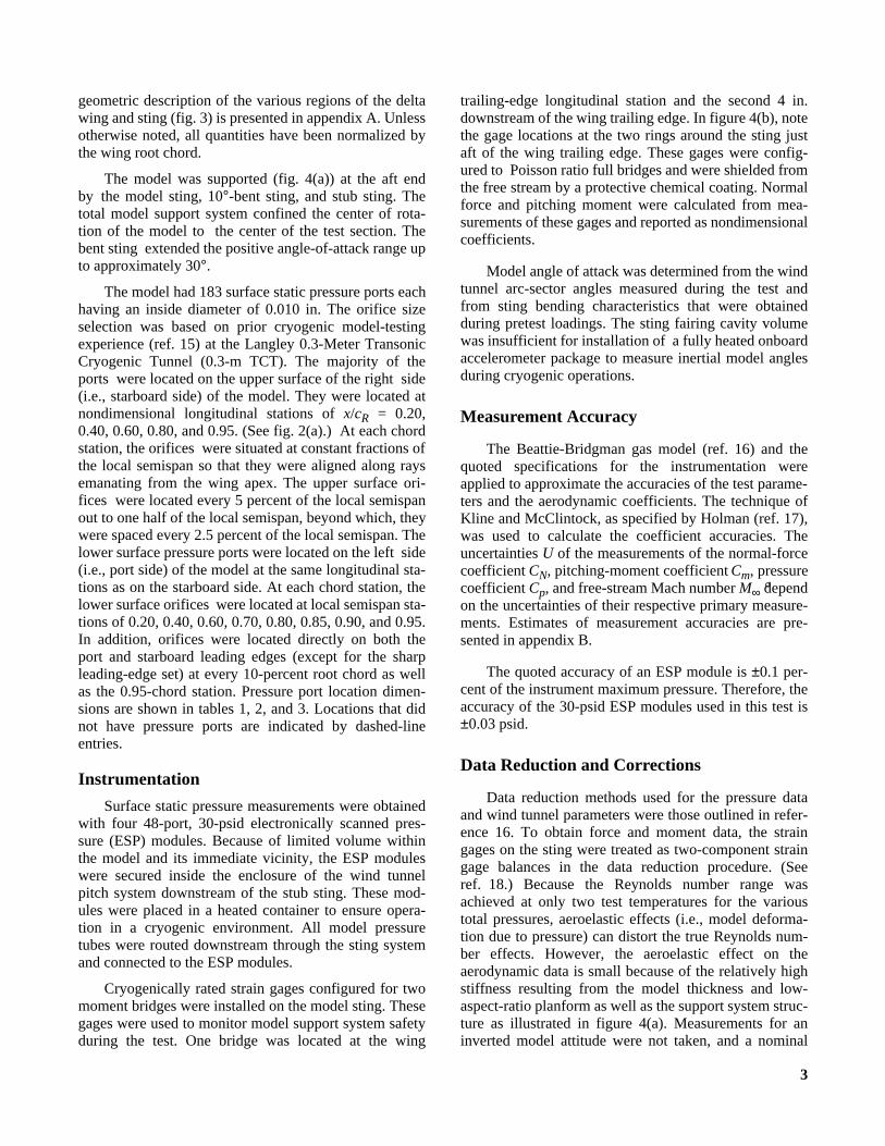
The test was conducted in the Langley NationalTransonic Facility (NTF). The facility is a fan-driven,closed-circuit, cryogenic transonic pressure wind tunnel.

(See fig. 1.) The test section is 8.2 ft high by 8.2 ft wideby 25 ft long with a slotted ceiling and floor.

The NTF operating capability has a nominal Machnumber range of 0.2 to 1.2, total pressure range of 15 to120 psia, and total temperature range of−260°F to150°F. The test gas may be dry air or nitrogen. A maxi-mum unit Reynolds number of 146× 106 ft−1 is achievedat a Mach number of 1.0. Independent control of pres-sure, temperature, fan speed, and inlet guide vane anglepermits Mach number, Reynolds number, and dynamicpressure to be varied independently within the wind tun-nel operational envelope.

To reduce turbulence, four antiturbulence screenswere installed in the settling chamber, and a 15:1 con-traction from settling chamber to nozzle throat was pro-vided. To minimize wall interference, the test sectionfloor and ceiling were set at 0°, model support walls at−1.76°, and reentry flaps at 0°. Acoustic treatmentupstream and downstream of the fan was incorporatedto reduce fan noise. More details of the wind tunnelphysical characteristics and operations can be found inreference 14.

Model Description and Test Apparatus

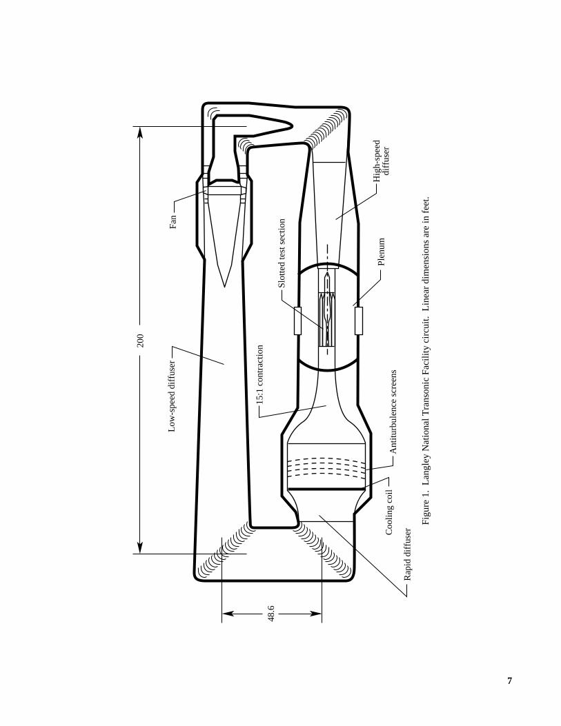
The basic layout of the delta wing model is shown infigure 2(a). The wing has a leading-edge sweep of 65°,no twist or camber, and four sets of interchangeable lead-ing edges, which attach to the flat plate part of the wing.The four leading-edge streamwise contours are illus-trated in figure 2(b). The model root chord is 25.734 in.,the wing span is 24 in., and the maximum wing thicknessis 0.875 in. The wing was fabricated from VascoMaxC-200,1 which is suitable for cryogenic operation, andhad a surface finish specification of 8 microinches.Figure2(c) is a photograph of three of the leading-edgesets; one set is attached to the flat plate part of the model.With the exception of the seam at the plane of symmetry,where the left and right side leading edges are joined,each interchangeable leading-edge set (which includespart of the outboard trailing edge) was fabricated as onecontinuous piece of hardware. This eliminated the sur-face discontinuity typically associated with an upper andlower leading-edge surface parting line.

The wing and sting surfaces are represented by afully analytical function with continuity through the sec-ond derivative and, hence, curvature. However, the wing-sting intersection line exhibits a discontinuity in slopeacross it. The leading- and trailing-edge cross-sectionalshapes are constant spanwise except for a region near thewingtip where the two shapes intersect. A detailed

1Trademark of Teledyne Vasco.

2ybι------

3

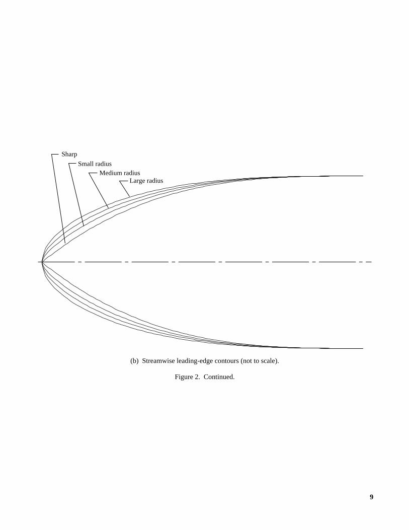
geometric description of the various regions of the deltawing and sting (fig. 3) is presented in appendix A. Unlessotherwise noted, all quantities have been normalized bythe wing root chord.

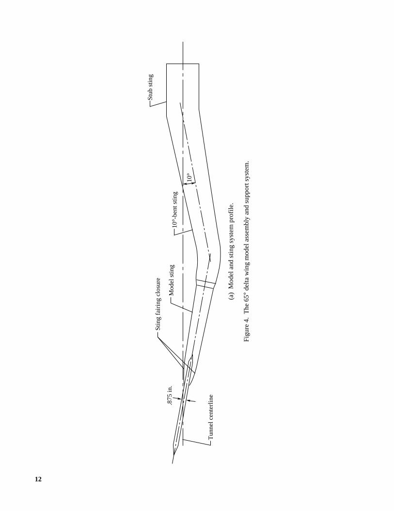
The model was supported (fig. 4(a)) at the aft endby the model sting, 10°-bent sting, and stub sting. Thetotal model support system confined the center of rota-tion of the model to the center of the test section. Thebent sting extended the positive angle-of-attack range upto approximately 30°.

The model had 183 surface static pressure ports eachhaving an inside diameter of 0.010 in. The orifice sizeselection was based on prior cryogenic model-testingexperience (ref. 15) at the Langley 0.3-Meter TransonicCryogenic Tunnel (0.3-m TCT). The majority of theports were located on the upper surface of the right side(i.e., starboard side) of the model. They were located atnondimensional longitudinal stations ofx/cR = 0.20,0.40, 0.60, 0.80, and 0.95. (See fig. 2(a).) At each chordstation, the orifices were situated at constant fractions ofthe local semispan so that they were aligned along raysemanating from the wing apex. The upper surface ori-fices were located every 5 percent of the local semispanout to one half of the local semispan, beyond which, theywere spaced every 2.5 percent of the local semispan. Thelower surface pressure ports were located on the left side(i.e., port side) of the model at the same longitudinal sta-tions as on the starboard side. At each chord station, thelower surface orifices were located at local semispan sta-tions of 0.20, 0.40, 0.60, 0.70, 0.80, 0.85, 0.90, and 0.95.In addition, orifices were located directly on both theport and starboard leading edges (except for the sharpleading-edge set) at every 10-percent root chord as wellas the 0.95-chord station. Pressure port location dimen-sions are shown in tables 1, 2, and 3. Locations that didnot have pressure ports are indicated by dashed-lineentries.

Instrumentation

Surface static pressure measurements were obtainedwith four 48-port, 30-psid electronically scanned pres-sure (ESP) modules. Because of limited volume withinthe model and its immediate vicinity, the ESP moduleswere secured inside the enclosure of the wind tunnelpitch system downstream of the stub sting. These mod-ules were placed in a heated container to ensure opera-tion in a cryogenic environment. All model pressuretubes were routed downstream through the sting systemand connected to the ESP modules.

Cryogenically rated strain gages configured for twomoment bridges were installed on the model sting. Thesegages were used to monitor model support system safetyduring the test. One bridge was located at the wing

trailing-edge longitudinal station and the second 4 in.downstream of the wing trailing edge. In figure 4(b), notethe gage locations at the two rings around the sting justaft of the wing trailing edge. These gages were config-ured to Poisson ratio full bridges and were shielded fromthe free stream by a protective chemical coating. Normalforce and pitching moment were calculated from mea-surements of these gages and reported as nondimensionalcoefficients.

Model angle of attack was determined from the windtunnel arc-sector angles measured during the test andfrom sting bending characteristics that were obtainedduring pretest loadings. The sting fairing cavity volumewas insufficient for installation of a fully heated onboardaccelerometer package to measure inertial model anglesduring cryogenic operations.

Measurement Accuracy

The Beattie-Bridgman gas model (ref. 16) and thequoted specifications for the instrumentation wereapplied to approximate the accuracies of the test parame-ters and the aerodynamic coefficients. The technique ofKline and McClintock, as specified by Holman (ref. 17),was used to calculate the coefficient accuracies. TheuncertaintiesU of the measurements of the normal-forcecoefficientCN, pitching-moment coefficientCm, pressurecoefficientCp, and free-stream Mach numberM∞ °dependon the uncertainties of their respective primary measure-ments. Estimates of measurement accuracies are pre-sented in appendix B.

The quoted accuracy of an ESP module is±0.1 per-cent of the instrument maximum pressure. Therefore, theaccuracy of the 30-psid ESP modules used in this test is±0.03 psid.

Data Reduction and Corrections

Data reduction methods used for the pressure dataand wind tunnel parameters were those outlined in refer-ence 16. To obtain force and moment data, the straingages on the sting were treated as two-component straingage balances in the data reduction procedure. (Seeref. 18.) Because the Reynolds number range wasachieved at only two test temperatures for the varioustotal pressures, aeroelastic effects (i.e., model deforma-tion due to pressure) can distort the true Reynolds num-ber effects. However, the aeroelastic effect on theaerodynamic data is small because of the relatively highstiffness resulting from the model thickness and low-aspect-ratio planform as well as the support system struc-ture as illustrated in figure 4(a). Measurements for aninverted model attitude were not taken, and a nominal

4

flow angularity correction of +0.13° (upflow) wasapplied to the reported angles of attack.

Test Program

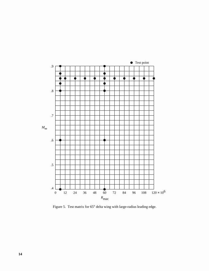
Figure 5 shows the combinations of Reynolds num-bers and free-stream Mach numbers used for the test. Thetest matrix shows that a Mach number of 0.85 wasselected for the study of the Reynolds number effects andthat Reynolds numbers of 6× 106 and 60× 106 wereselected for the study of the Mach number effects. Alldata were obtained with free boundary layer transition.

Data Presentation

Pressure data measured on the delta wing are pre-sented for each data point in tabular and graphical for-mats in appendixes C–E. Normal-force and pitching-moment data for each angle of attack are presented infigures 6–8. The moment reference point was located attwo thirds of the root chord aft of the wing apex. Theangle of attack ranged nominally from−1° to 27°.

Wing pressure coefficients are tabulated for eachdata point and accompanied by a surface pressure distri-bution plot and a leading-edge pressure plot. The degreeof similarity between the port and starboard leading-edgepressure plots indicates the extent of flow symmetry.Note that a coefficient value represented by a seriesof asterisks in tables C1–C11, D1–D6, and E1–E6 iseither anunrecorded or an apparently erroneous pressureport measurement.

The pressure coefficient data test matrix is presentedin table 4. The test breakdown is as follows: datafor Reynolds numbers from 6× 106 to 120× 106 atM∞ = 0.85 are given in appendix C, data for a Reynoldsnumber of 6× 106 at M∞ = 0.40 to 0.90 are given inappendix D, and data for a Reynolds number of 60× 106

atM∞ = 0.40 to 0.90 are given in appendix E.

Summary Remarks

Pressure data obtained from a 65° delta wing withthe large-radius leading edge (i.e., 0.30 percent of mac)are presented in the form of surface pressure plots andleading-edge pressure plots for a Reynolds number rangeat a Mach number of 0.85 and a Mach number range atReynolds numbers of 6× 106 and 60× 106. Althoughupper and lower surface pressures were measured onopposite sides of the model, model symmetry permittedpressure distribution plots to be superimposed on asketch of the half wing. The plots of the leading-edgepressures indicate the extent of flow symmetry by com-paring port and starboard leading-edge pressures.Normal-force and pitching-moment coefficient plots forReynolds number and Mach number ranges are alsopresented.

NASA Langley Research CenterHampton, VA 23681-0001August 11, 1995

5

Table 1. Wing Upper Surface Pressure Port Locations on Starboard Side

x/cR of—0.20 0.40 0.60 0.80 0.95

η x, in. y, in. x, in. y, in. x, in. y, in. x, in. y, in. x, in. y, in.0.050 5.147 0.120 10.294 0.240 15.440 0.360 ------ ------ ------ ------.100 .240 .480 .720 ------ ------ ------ ------.150 .360 .720 1.080 ------ ------ ------ ------.200 .480 .960 1.440 ------ ------ 24.447 2.280.250 ------ ------ 1.200 1.800 20.587 2.400 2.850.300 5.147 0.720 1.440 2.160 2.880 3.420.350 .840 1.680 2.520 3.360 3.990.400 .960 1.920 2.880 3.840 4.560.450 1.080 2.160 3.240 4.320 5.130.500 1.200 2.400 3.600 4.800 5.700.525 ------ ------ 2.520 3.780 5.040 5.985.550 5.147 1.320 2.640 3.960 5.280 6.270.575 ------ ------ 2.760 4.140 5.520 6.550.600 5.147 1.440 2.880 4.320 5.760 6.840.625 ------ ------ ------ ------ 4.500 6.000 7.125.650 5.147 1.560 10.294 3.120 4.680 6.240 7.410.675 ------ ------ 3.240 4.860 6.480 7.695.700 5.147 1.680 3.360 5.040 6.720 7.980.725 ------ ------ 3.480 5.220 6.960 8.265.750 5.147 1.800 3.600 ------ ------ 7.200 8.550.775 ------ ------ 3.720 15.440 5.580 7.440 8.835.800 5.147 1.920 3.840 5.760 7.680 9.120.825 ------ ------ 3.960 5.940 7.920 9.405.850 5.147 2.040 4.080 6.120 8.160 9.690.875 ------ ------ 4.200 6.300 8.400 9.975.900 5.147 2.160 4.320 6.480 8.640 10.260.925 ------ ------ 4.440 6.660 8.880 10.545.950 5.147 2.280 4.560 6.840 9.120 10.830.975 ------ ------ 4.680 7.020 9.360 11.115

1.000 5.147 2.280 4.800 7.200 9.600 11.400

6

Table 2. Wing Lower Surface Pressure Port Locations on Port Side

x/cR of—0.20 0.40 0.60 0.80 0.95

η x, in. y, in. x, in. y, in. x, in. y, in. x, in. y, in. x, in. y, in.−0.200 5.147 −0.480 10.294 −0.960 15.440 −1.440 ------ ------ 24.447 −2.280−.400 −.960 −1.920 −2.880 20.587 −3.840 −4.560−.600 −1.440 −2.880 −4.320 −5.760 −6.840−.700 −1.680 −3.360 −5.040 −6.720 −7.980−.800 −1.920 −3.840 −5.760 −7.680 −9.120−.850 −2.040 −4.080 −6.120 −8.160 −9.690−.900 −2.160 −4.320 −6.480 −8.640 −10.260−.950 −2.280 −4.560 −6.840 −9.120 −10.830−.975 ------ ------ −4.680 −7.020 −9.360 −11.115

−1.000 5.147 −2.400 −4.800 −7.200 −9.600 −11.400

Table 3. Wing Leading-Edge Pressure Port Locations on Starboard Side

x/cR of—0.10 0.30 0.50 0.70 0.90

η x, in. y, in. x, in. y, in. x, in. y, in. x, in. y, in. x, in. y, in.1.000 2.573 1.200 7.720 3.600 12.867 6.000 18.014 8.400 23.161 10.800

Table 4. Pressure Coefficient Data Test Matrix for Large-Radius Leading Edge

Appendix table Run Mach Rmac q∞, psf tT, °FC1 80 0.85 6× 106 722 120C2 57 12 1444 120C3 63 24 690 −250C4 64 36 1035C5 65 48 1380C6 66 60 1725C7 67 72 2068C8 78 84 2413C9 70 96 2756C10 69 108 3099C11 68 120 3442D1 58 0.40 6 387 120D2 59 .60 555D3 60 .80 692D4 79 .83 710D5 81 .87 733D6 82 .90 750E1 77 .40 60 950 −250E2 76 .60 1344E3 75 .80 1659E4 72 .83 1699E5 73 .87 1749E6 74 .90 1785

7

Fig

ure

1. L

angl

ey N

atio

nal T

rans

onic

Fac

ility

circ

uit.

Lin

ear

dim

ensi

ons

are

in fe

et.

200

Fan

Low

-spe

ed d

iffu

ser

15:1

con

trac

tion

Slot

ted

test

sec

tion

Hig

h-sp

eed

diff

user

Plen

umA

ntitu

rbul

ence

scr

eens

Coo

ling

coil

Rap

id d

iffu

ser

48.6

8

(a) Model configuration.

Figure 2. Delta wing model.

0

.2

.4

.6

.8

1.0

.2 .4 .6y/cR

x/cR

65°

Interchangeable leading edge

Pressure station (5 places)

Flat plate

Sting fairing

Trailing-edge closure region

y/cR = 0.466

9

(b) Streamwise leading-edge contours (not to scale).

Figure 2. Continued.

Sharp

Small radiusMedium radius

Large radius

10

L-88

-991

1(c

) M

odel

with

thre

e le

adin

g-ed

ge s

ets.

Fig

ure

2. C

oncl

uded

.

11

Figure 3. Delta wing model fore-sting detail.

0

.6

.8

1.0

1.2

1.4

.2 .4 .6y/cR

x/cR

1.6

1.8

0.9797

1.175

1.253

1.684

1.7580° taper

2.25° taper

0° taper Region 1

Region 2

Region 3

Region 4

r/cR = 1.979

y/cR = 0.466

12

(a)

Mod

el a

nd s

ting

syst

em p

rofil

e.

Fig

ure

4. T

he 6

5° de

lta w

ing

mod

el a

ssem

bly

and

supp

ort s

yste

m.

Stin

g fa

irin

g cl

osur

e

Mod

el s

ting

10°-

bent

stin

g

Stub

stin

g

10°

.875

in.

Tun

nel c

ente

rlin

e

13

L-91

-696

3(b

) In

stal

latio

n in

Lan

gley

Nat

iona

l Tra

nson

ic F

acili

ty.

Fig

ure

4. C

oncl

uded

.

14

Figure 5. Test matrix for 65° delta wing with large-radius leading edge.

0 12 24 36 48 60 72 84 96 108 120 × 106

Rmac

.4

.5

.6

.7

.8

.9

M∞

Test point

15

(a) CN versusα.

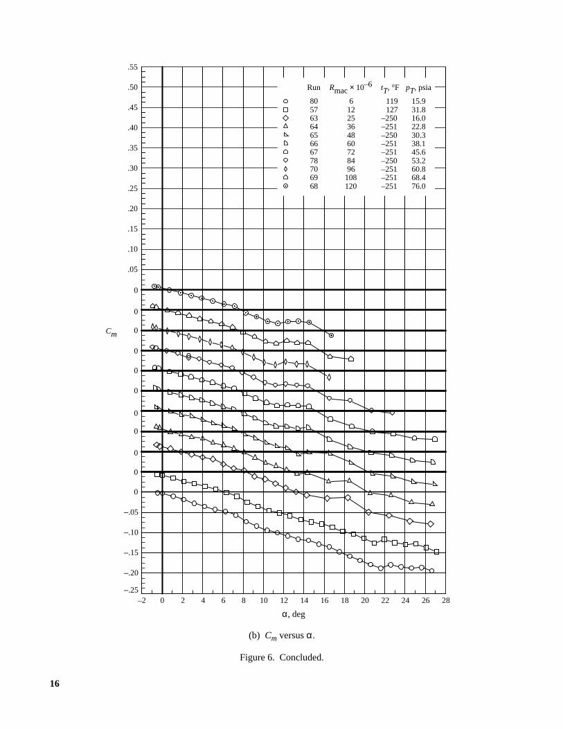
Figure 6. Normal-force and pitching-moment coefficients at angles of attack for wing with large-radius leading edge.M∞ ≈ 0.85.

–.2

0

.2

.4

.6

.8

1.0

1.2

1.4

1.6

1.8

2.0

2.2

2.4

2.6

2.8

–2 0 2 4 6 8 10 12 14 16 18 20 22 24 26 28

α, deg

CN

0

0

0

0

0

0

0

0

0

0

80 57 63 64 65 66 67 78 70 69 68

6 12 25 36 48 60 72 84 96

108 120

119 127

–250 –251 –250 –251 –251 –250 –251 –251 –251

15.9 31.816.0 22.830.3 38.1 45.653.2 60.8 68.476.0

Run Rmac × 10–6 tT, °F pT, psia

16

(b) Cm versusα.

Figure 6. Concluded.

–.25

–.20

–.15

–.10

–.05

0

.05

.10

.15

.20

.25

.30

.35

.40

.45

.50

.55

–2 0 2 4 6 8 10 12 14 16 18 20 22 24 26 28

α, deg

Cm

0

0

0

0

0

0

0

0

0

0

80 57 63 64 65 66 67 78 70 69 68

6 12 25 36 48 60 72 84 96

108 120

119 127

–250 –251 –250 –251 –251 –250 –251 –251 –251

15.9 31.816.0 22.830.3 38.1 45.653.2 60.8 68.476.0

Run Rmac × 10–6 tT, °F pT, psia

17

(a) CN versusα.

Figure 7. Normal-force and pitching-moment coefficients at angles of attack for wing with large-radius leading edge.Rmac≈ 6 × 106.

–.2

0

.2

.4

.6

.8

1.0

1.2

1.4

1.6

1.8

2.0

2.2

2.4

2.6

2.8

–2 0 2 4 6 8 10 12 14 16 18 20 22 24 26 28

α, deg

CN

0

0

0

0

0

0

58 59 60 79 80 81 82

0.40 .60 .80 .83 .85 .87 .90

118 119 121 121 119 120 120

26.8 19.516.3 16.115.9 15.7 15.5

Run tT, °F pT, psiaM∞

18

(b) Cm versusα.

Figure 7. Concluded.

–.25

–.20

–.15

–.10

–.05

0

.05

.10

.15

.20

.25

.30

.35

.40

.45

.50

.55

–2 0 2 4 6 8 10 12 14 16 18 20 22 24 26 28

α, deg

Cm

0

0

0

0

0

0

58 59 60 79 80 81 82

0.40 .60 .80 .83 .85 .87 .90

118 119 121 121 119 120 120

26.8 19.516.3 16.115.9 15.7 15.5

Run tT, °F pT, psiaM∞

19

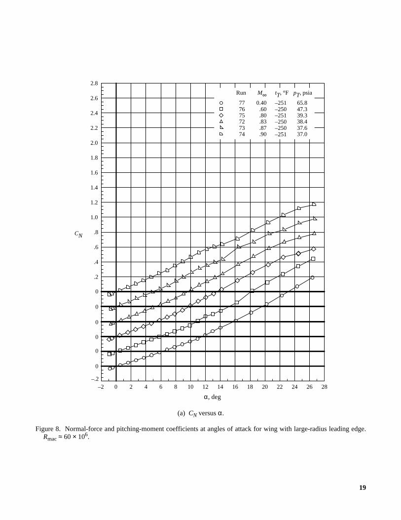
(a) CN versusα.

Figure 8. Normal-force and pitching-moment coefficients at angles of attack for wing with large-radius leading edge.Rmac≈ 60 × 106.

–.2

0

.2

.4

.6

.8

1.0

1.2

1.4

1.6

1.8

2.0

2.2

2.4

2.6

2.8

–2 0 2 4 6 8 10 12 14 16 18 20 22 24 26 28

α, deg

CN

0

0

0

0

0

77 76 75 72 73 74

0.40 .60 .80 .83 .87 .90

–251 –250 –251 –250 –250 –251

65.8 47.339.3 38.437.6 37.0

Run tT, °F pT, psiaM∞

20

(b) Cm versusα.

Figure 8. Concluded.

–.25

–.20

–.15

–.10

–.05

0

.05

.10

.15

.20

.25

.30

.35

.40

.45

.50

.55

–2 0 2 4 6 8 10 12 14 16 18 20 22 24 26 28

α, deg

Cm

0

0

0

0

0

77 76 75 72 73 74

0.40 .60 .80 .83 .87 .90

–251 –250 –251 –250 –250 –251

65.8 47.339.3 38.437.6 37.0

Run tT, °F pT, psiaM∞

21

Appendix A

Delta Wing and Near-Field Sting AnalyticalDefinition

General equations were used to define the leading-edge semithickness, the flat plate semithickness, thetrailing-edge closure semithickness, and the transverseradius of the sting fairing. The equationϕ defines theparticular shape of interest (e.g., the leading-edge con-tour) and the equationψ defines the boundary conditions(at ξ = 1) forϕ. Details are as follows:

(A1)

(A2)

(A3)

The second-blending functionψ is defined such that

The two functionsϕ and ψ are illustrated in figure A1 forthe leading-edge semithickness case wherex0 = xle.

The general analytical expressions for the coeffi-cients in equation (A2) follow:

With these expressions

and the leading-edge radius atξ = 0 is r. Curvature isalso continuous atξ = 1.

For the delta wing model of this study, the flat platepart represented byψ results in bothm andn being zero.The reduced coefficients are

For a sharp leading edge, the radiusr = 0 and thecoefficients further reduce to

Specific numerical values follow for the delta wing insubsequent discussions.

Leading Edges

The streamwise leading-edge contours are designedto give leading-edge radii of 0, 0.05, 0.15, and 0.30 per-cent of the mean aerodynamic chord and to match the flatplate wing at a streamwise distance of 15 percent of theroot chord aft of the leading edge with continuity throughthe second derivative. The longitudinal coordinate ofthe leading edge isxle and the leading-edge contour isdescribed by equation (A2), the coefficients in table A1,and the following definitions:

Flat Plate

The flat plate center part of the wing has a uniformthickness. The equation for the semithickness is asfollows:

ξ x x0–( ) x1⁄=

ϕ ξ( ) x1 a ξ bξ cξ2dξ3

+ + + ±= 0 ξ 1≤ ≤( )

ψ ξ( ) x1± lx1----- m ξ 1–( )

nx1

2-------- ξ 1–( )2

+ += 1 ξ≤( )

ψ ξ 1=l= dψ

dx-------

ξ 1=

m= d2ψ

dx2

----------

ξ 1=

n=

a2rx1-----=

b158------a 3

lx1----- 2m–

nx1

2--------++–=

c54---a 3

lx1-----– 3m nx1–+=

d38---a– l

x1----- m–

nx1

2--------++=

ϕ 1( ) ψ 1( )= ϕ′ 1( ) ψ′ 1( )= ϕ′′ 1( ) ψ′′ 1( )=

a2rx1-----=

b158------a 3

lx1-----+–=

c54---a 3

lx1-----–=

d38---a– l

x1-----+=

a 0=

b 3l

x1-----=

c 3l

x1-----–=

dl

x1-----=

x0 xle=

x1 0.15=

x0 xle 0.15+=

x1 0.9 x0–=

ϕ ξ( ) 0.0170008±= 0 ξ 1≤ ≤( )

22

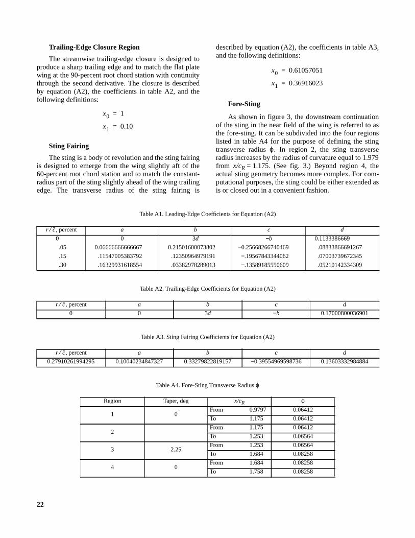
Trailing-Edge Closure Region

The streamwise trailing-edge closure is designed toproduce a sharp trailing edge and to match the flat platewing at the 90-percent root chord station with continuitythrough the second derivative. The closure is describedby equation (A2), the coefficients in table A2, and thefollowing definitions:

Sting Fairing

The sting is a body of revolution and the sting fairingis designed to emerge from the wing slightly aft of the60-percent root chord station and to match the constant-radius part of the sting slightly ahead of the wing trailingedge. The transverse radius of the sting fairing is

described by equation(A2), the coefficients in table A3,and the following definitions:

Fore-Sting

As shown in figure 3, the downstream continuationof the sting in the near field of the wing is referred to asthe fore-sting. It can be subdivided into the four regionslisted in table A4 for the purpose of defining the stingtransverse radiusϕ. In region 2, the sting transverseradius increases by the radius of curvature equal to 1.979from x/cR = 1.175. (See fig. 3.) Beyond region 4, theactual sting geometry becomes more complex. For com-putational purposes, the sting could be either extended asis or closed out in a convenient fashion.

x0 1=

x1 0.10=

x0 0.61057051=

x1 0.36916023=

Table A1. Leading-Edge Coefficients for Equation (A2)

, percent a b c d

0 0 3d −b 0.1133386669

.05 0.06666666666667 0.21501600073802 −0.25668266740469 .08833866691267

.15 .11547005383792 .12350964979191 −.19567843344062 .07003739672345

.30 .16329931618554 .03382978289013 −.13589185550609 .05210142334309

Table A2. Trailing-Edge Coefficients for Equation (A2)

, percent a b c d

0 0 3d −b 0.17000800036901

Table A3. Sting Fairing Coefficients for Equation (A2)

, percent a b c d

0.27910261994295 0.10040234847327 0.33279822819157 −0.39554969598736 0.13603332984884

Table A4. Fore-Sting Transverse Radiusϕ

Region Taper, deg x/cR ϕ

1 0From 0.9797 0.06412

To 1.175 0.06412

2From 1.175 0.06412

To 1.253 0.06564

3 2.25From 1.253 0.06564

To 1.684 0.08258

4 0From 1.684 0.08258

To 1.758 0.08258

r c⁄

r c⁄

r c⁄

23

Fig

ure

A1.

Del

ta w

ing

sem

ithic

knes

s fu

nctio

ns.

Z

X

ϕ (ξ

)

ψ (ξ

)

x 1

x 0 = x

le

r le

ξ =

1ξ

= 0

ξ =

(x–

x 0)/x 1

24

Appendix B

Data Uncertainty

The uncertaintiesU of the measurements of thenormal-force coefficientCN, pitching-moment coeffi-cient Cm, pressure coefficientCp, and free-stream MachnumberM∞ depend on the uncertainties of their respec-tive primary measurements.

The coefficientsCN, Cm, andCp (Mach number isdiscussed separately) are derived by

(B1)

(B2)

(B3)

The primary measurements used to define thesecoefficients are the normal forceFN, pitching momentMY, surface local static pressurep, free-stream staticpressurep∞, and free-stream total pressurepT. The free-stream static pressure and the free-stream total pressureare used to compute the free-stream Mach number,which, in turn, is used to compute the free-streamdynamic pressureq∞.

The free-stream dynamic pressure that accounts forthe compressibility effect in high-speed flow is definedas

(B4)

whereγ denotes the ratio of specific heats. Substitutionsfor the dynamic pressure in the normal-force, pitching-moment, and pressure coefficient equations (B1), (B2),and (B3), respectively, give

(B5)

(B6)

(B7)

The Mach number, which is not a primary measurement,is derived from the free-stream static and total pressuresand the ratio of specific heats. Thus,

(B8)

The coefficients are then functions of the followingmeasured variables: the normal force, the pitchingmoment, the local pressure, the free-stream static pres-sure, and the free-stream Mach number; the Mach num-ber is a function of the free-stream static pressure and thefree-stream total pressure (i.e., stagnation pressure). TheuncertaintiesU( ) of these primary measured variablesare presented in table B1.

The probability of the value of each uncertaintybeing correct is assumed to be the same. From refer-ence17, the uncertainty for each of the coefficients ofequations (B5)–(B8) with the same probability is

(B9)

(B10)

(B11)

(B12)

CN

FN

q∞S----------=

Cm

MY

q∞Sc-------------=

Cp

p p∞–

q∞----------------=

q∞12---γ p∞M∞

2=

CN

FN

12---γ p∞M∞

2S

--------------------------=

Cm

MY

12---γ p∞M∞

2Sc

-----------------------------=

Cp

p p∞–

12---γ p∞M∞

2-----------------------=

Table B1. Data Uncertainties

Variable Uncertainty

U(FN), lbf . . . . . . . . . . . . . . . <24.0

U(MY), in-lbf . . . . . . . . . . . . <46.8

U(p), lbf/in2 . . . . . . . . . . . . . <0.03

U(pT), lbf/in2 . . . . . . . . . . . . <0.01

U(p∞), lbf/in2 . . . . . . . . . . . . <0.02

M∞2

γ 1–-----------

p∞pT-------

γ 1–( )– γ⁄

1– 1 2⁄

=

U CN( )CN∂FN∂

---------- U FN( )2

CN∂p∞∂

---------- U p∞( )2

+

=

CN∂M∞∂

----------- U M∞( )2

1 2⁄

+

U Cm( )Cm∂MY∂

----------- U MY( )2

Cm∂p∞∂

---------- U p∞( )2

+

=

Cm∂M∞∂

----------- U M∞( )2

1 2⁄

+

U Cp( )Cp∂p∂

---------- U p( )2

Cp∂p∞∂

---------- U p∞( )2

+

=

Cp∂M∞∂

----------- U M∞( )2

1 2⁄

+

U M∞( )M∞∂p∞∂

----------- U p∞( )2

M∞∂pT∂

----------- U pT( )2

+

1 2⁄

=

25

Equations (B5)–(B8) are used to obtain the sensitivity ofthe derived quantity with respect to each of the primarymeasurements. The uncertainty in Mach number is firstdetermined with the nominal wind tunnel static and totalpressures for representative Reynolds and Mach num-bers. The sensitivity factors (i.e., quantities in partialderivatives) change as the values of the primary measure-

ments change based on test Reynolds and Mach num-bers. The contributions of the static pressure and totalpressure measurement to the calculated uncertainty inMach number, normal-force coefficient, pitching-moment coefficient, and pressure coefficient are listed intables B2–B5.

Table B2. Contribution of Primary Measurements to Mach Number Uncertainty

M∞ Rmac pT, psia tT, °F U (M∞)

0.40 6× 106 66 120 −0.0004 0.0002 0.0005

.60 6 19.5 120 −.0003 .0002 .0003

.85 120 76 −250 −.0002 .0001 .0003

.90 6 15.5 120 −.0003 .0001 .0003

Table B3. Contribution of Primary Measurements to Normal-Force Coefficient Uncertainty

M∞ Rmac pT, psia tT, °F α, deg U (CN)

0.40 6× 106 66.0 120

4.84 0.01187 −0.00003 0.00037 0.0119

9.95 0.01189 −0.00008 −0.00080 0.0119

20.17 0.01189 −0.00019 −0.00202 0.0121

0.60 6× 106 19.5 120

4.99 0.02020 −0.00004 −0.00019 0.0202

10.14 0.02020 −0.00009 −0.00045 0.0202

20.26 0.02021 −0.00022 −0.00106 0.0202

0.85 120× 106 76.0 −250

4.95 0.00323 −0.00005 −0.00012 0.0032

10.34 0.00322 −0.00012 −0.00030 0.0032

14.57 0.00323 −0.00017 −0.00044 0.0033

0.90 6× 106 15.5 120

5.06 0.01501 −0.00007 −0.00015 0.0150

10.20 0.01500 −0.00016 −0.00034 0.0150

20.33 0.01503 −0.00034 −0.00074 0.0150

M∞∂p∞∂

----------- U p∞( )M∞∂pT∂

----------- U pT( )

CN∂FN∂

---------- U FN( )CN∂p∞∂

---------- U p∞( )CN∂M∞∂

----------- U M∞( )

26

Table B4. Contribution of Primary Measurements to Pitching-Moment Coefficient Uncertainty

M∞ Rmac pT, psia tT, °F α, deg U (Cm)

0.40 6× 106 66.0 120

4.84 0.00000 0.00000 0.00005 0.0000

9.95 0.00000 0.00001 0.00012 0.0001

20.17 0.00000 0.00003 0.00027 0.0003

0.60 6× 106 19.5 120

4.99 0.00000 0.00001 0.00003 0.0000

10.14 0.00000 0.00001 0.00007 0.0001

20.26 0.00000 0.00003 0.00014 0.0001

0.85 120× 106 76.0 −250

4.95 0.00000 0.00001 0.00002 0.0000

10.34 0.00000 0.00002 0.00005 0.0001

14.57 0.00000 0.00003 0.00006 0.0001

0.90 6× 106 15.5 120

5.06 0.00000 0.00001 0.00003 0.0000

10.20 0.00000 0.00003 0.00007 0.0001

20.33 0.00000 0.00007 0.00015 0.0002

Table B5. Contribution of Primary Measurements to Pressure Coefficient Uncertainty

M∞ Rmac pT, psia tT, °F α, deg U (Cp)

0.40 6× 106 66.0 120

4.84 0.00458 0.00001 0.01066 0.0116

9.95 0.00459 0.00002 0.01077 0.0117

20.17 0.00459 0.00007 0.01101 0.0119

0.60 6× 106 19.5 120

4.99 0.00780 0.00002 0.00231 0.0081

10.14 0.00780 0.00005 0.00238 0.0082

20.26 0.00780 0.00010 0.00249 0.0082

0.85 120× 106 76.0 −250

4.95 0.00125 0.00000 0.00062 0.0014

10.34 0.00124 0.00001 0.00062 0.0014

14.57 0.00125 0.00001 0.00063 0.0014

0.90 6× 106 15.5 120

5.06 0.00580 0.00002 0.00064 0.0058

10.20 0.00579 0.00006 0.00068 0.0058

20.33 0.00580 0.00007 0.00070 0.0058

Cm∂MY∂

----------- U MY( )Cm∂p∞∂

---------- U p∞( )Cm∂M∞∂

----------- U M∞( )

Cp∂p∂

---------- U p( )Cp∂p∞∂

---------- U p∞( )Cp∂M∞∂

----------- U M∞( )

27

Appendix C

Experimental Surface Pressure Data for 65° Delta Wing, M∞ = 0.85

The experimental surface pressure data for the 65° delta wing at constantM∞ = 0.85 are summarized in tables C1–C11. Because of the extensive data contained in these tables, they have not been included in the printed copy of thepaper but are available electeonically from the Langley Technical Report Server (LTRS). Open the files with the follow-ing Uniform Resource Locator (URL):

ftp://techreports.larc.nasa.gov/pub/techreports/larc/96/NASA-96-tm4645vol4appC.ps.Z

28

Appendix D

Experimental Surface Pressure Data for 65° Delta Wing, Rmac = 6 × 106

The experimental surface pressure data for the 65° delta wing at constantRmac= 6 × 106 are summarized intablesD1–D6. Because of the extensive data contained in these tables, they have not been included in the printed copyof the paper but are available electronically from the Langley Technical Report Server (LTRS). Open the files with thefollowing Uniform Resource Locator (URL):

ftp://techreports.larc.nasa.gov/pub/techreports/larc/96/NASA-96-tm4645vol4appD.ps.Z

29

Appendix E

Experimental Surface Pressure Data for 65° Delta Wing, Rmac = 60× 106

The experimental surface pressure data for the 65° delta wing at constantRmac= 60× 106 are summarized intablesE1–E6. Because of the extensive data contained in these tables, they have not been included in the printed copy ofthe paper but are available electronically from the Langley Technical Report Server (LTRS). Open the files with the fol-lowing Uniform Resource Locator (URL):

ftp://techreports.larc.nasa.gov/pub/techreports/larc/96/NASA-96-tm4645vol4appE.ps.Z

30

References1. Winter, H.: Flow Phenomena on Plates and Airfoils of Short

Span. NACA TM-798, 1936.

2. Wilson, Herbert A.; and Lovell, J. Calvin:Full-Scale Investi-gation of the Maximum Lift and Flow Characteristics ofan Airplane Having Approximately Triangular Plan Form.NACA RM L6K20, 1947.

3. Örnberg, Torsten:A Note On the Flow Around Delta Wings.KTH-Aero TN 38, Div. of Aeronautics, R. Inst. of Technology(Stockholm), 1954.

4. Lawford, J. A.: Low-Speed Wind Tunnel Experiments on aSeries of Sharp-Edged Delta Wings—Part II. Surface FlowPatterns and Boundary Layer Transition Measurements. Tech.Note Aero. 2954, R. Aircr. Establ., Mar. 1964.

5. Hummel, Ing. Dietrich: On the Vortex Formation Over a Slen-der Wing at Large Angles of Incidence.High Angle of AttackAerodynamics, AGARD-CP-247, Jan. 1979, pp. 15-1–15-17.

6. Vorropoulos, G.; and Wendt, J. F.: Laser Velocimetry Study ofCompressibility Effects on the Flow Field of a Delta Wing.Aerodynamics of Vortical Type Flows in Three Dimensions,AGARD-CP-342, July 1983, pp. 9-1–9-13. (Available fromDTIC as AD A135 157.)

7. Poisson-Quinton, P.: Slender Wings for Civil and Military Air-craft. Israel J. Technol. , vol. 16, no. 3, 1978, pp. 97–131.

8. Skow, A. M.; and Erickson, G. E.: Modern Fighter Air-craft Design for High-Angle-of-Attack Maneuvering. HighAngle-of-Attack Aerodynamics, AGARD-LS-121, Dec. 1982,pp. 4-1–4-59.

9. Polhamus, E. C.: Applying Slender Wing Benefits to MilitaryAircraft. J. Aircr., vol. 21, no. 8, Aug. 1984, pp. 545–559.

10. Polhamus, E. C.; and Gloss, B. B.: Configuration Aerodynam-ics. High Reynolds Number Research, NASA CP-2183, 1980,pp. 217–234.

11. Henderson, William P.: Effects of Wing Leading-Edge Radiusand Reynolds Number on Longitudinal Aerodynamic Charac-teristics of Highly Swept Wing-Body Configurations at Sub-sonic Speeds. NASA TN D-8361, 1976.

12. Howe, J. T.:Some Fluid Mechanical Problems Related to Sub-sonic and Supersonic Aircraft. NASA SP-183, 1969.

13. Henderson, William P.: Studies of Various Factors AffectingDrag Due to Lift at Subsonic Speeds. NASA TN D-3584,1966.

14. Fuller, Dennis E.:Guide for Users of the National TransonicFacility. NASA TM-83124, 1981.

15. Plentovich, E. B.:The Application to Airfoils of a Techniquefor Reducing Orifice-Induced Pressure Error at High ReynoldsNumbers. NASA TP-2537, 1986.

16. Hall, Robert M.; and Adcock, Jerry B.:Simulation of Ideal-Gas Flow by Nitrogen and Other Selected Gases at CryogenicTemperatures. NASA TP-1901, 1981.

17. Holman, Jack Philip:Experimental Methods for Engineers.4th ed., McGraw-Hill Book Co., 1984, pp. 46–99.

18. Foster, Jean M.; and Adcock, Jerry B.:User’s Guide for theNational Transonic Facility Data System. NASA TM-100511,1987.

Form ApprovedOMB No. 0704-0188

Public reporting burden for this collection of information is estimated to average 1 hour per response, including the time for reviewing instructions, searching existing data sources,gathering and maintaining the data needed, and completing and reviewing the collection of information. Send comments regarding this burden estimate or any other aspect of thiscollection of information, including suggestions for reducing this burden, to Washington Headquarters Services, Directorate for Information Operations and Reports, 1215 JeffersonDavis Highway, Suite 1204, Arlington, VA 22202-4302, and to the Office of Management and Budget, Paperwork Reduction Project (0704-0188), Washington, DC 20503.

1. AGENCY USE ONLY (Leave blank) 2. REPORT DATE 3. REPORT TYPE AND DATES COVERED

4. TITLE AND SUBTITLE 5. FUNDING NUMBERS

6. AUTHOR(S)

7. PERFORMING ORGANIZATION NAME(S) AND ADDRESS(ES)

9. SPONSORING/MONITORING AGENCY NAME(S) AND ADDRESS(ES)

11. SUPPLEMENTARY NOTES

8. PERFORMING ORGANIZATIONREPORT NUMBER

10. SPONSORING/MONITORINGAGENCY REPORT NUMBER

12a. DISTRIBUTION/AVAILABILITY STATEMENT 12b. DISTRIBUTION CODE

13. ABSTRACT (Maximum 200 words)

14. SUBJECT TERMS

17. SECURITY CLASSIFICATIONOF REPORT

18. SECURITY CLASSIFICATIONOF THIS PAGE

19. SECURITY CLASSIFICATIONOF ABSTRACT

20. LIMITATIONOF ABSTRACT

15. NUMBER OF PAGES

16. PRICE CODE

NSN 7540-01-280-5500 Standard Form 298 (Rev. 2-89)Prescribed by ANSI Std. Z39-18298-102

REPORT DOCUMENTATION PAGE

February 1996 Technical Memorandum

Experimental Surface Pressure Data Obtained on 65° Delta Wing AcrossReynolds Number and Mach Number RangesVolume 4—Large-Radius Leading Edge

WU 505-59-54-01

Julio Chu and James M. Luckring

L-17411D

NASA TM-4645, Vol. 4

An experimental wind tunnel test of a 65° delta wing model with interchangeable leading edges was conducted inthe Langley National Transonic Facility (NTF). The objective was to investigate the effects of Reynolds and Machnumbers on slender-wing leading-edge vortex flows with four values of wing leading-edge bluntness. Experimen-tally obtained pressure data are presented without analysis in tabulated and graphical formats across a Reynoldsnumber range of 6× 106 to 120× 106 at a Mach number of 0.85 and across a Mach number range of 0.4 to 0.9 atReynolds numbers of 6× 106 and 60× 106. Normal-force and pitching-moment coefficient plots for these Rey-nolds number and Mach number ranges are also presented.

Aerodynamics; Delta wing; Reynolds number; Leading-edge bluntness; Vortex flow;Cryogenic testing

31

A03

NASA Langley Research CenterHampton, VA 23681-0001

National Aeronautics and Space AdministrationWashington, DC 20546-0001

Unclassified–UnlimitedSubject Category 02Availability: NASA CASI (301) 621-0390

Unclassified Unclassified Unclassified