experimental study of water droplet flows in a model pem

Experimental Study of Water Droplet Flows in a Model PEM Fuel Cell Gas

Microchannel

by

Grant Minor

B. Eng. Mgmt., McMaster University, 2005

A Thesis Submitted in Partial Fulfillment of the

Requirements for the Degree of

MASTER OF APPLIED SCIENCE

in the Department of Mechanical Engineering

© Grant F. Minor, 2007

University of Victoria

All rights reserved. This thesis may not be reproduced in whole or in part,

by photocopy or other means, without permission of the author.

ii

Supervisory Committee

Experimental Study of Water Droplet Flows in a Model PEM Fuel Cell Gas

Microchannel

by

Grant Minor

B. Eng. Mgmt., McMaster University, 2005

Dr. Peter Oshkai, Co-Supervisor

(Department of Mechanical Engineering)

Dr. Ned Djilali, Co-Supervisor

(Department of Mechanical Engineering).

Dr. David Sinton, Co-Supervisor

(Department of Mechanical Engineering).

iii

Dr. Peter Oshkai, (Co-Supervisor, Mechanical Engineering).

Dr. Ned Djilali, (Co-Supervisor, Mechanical Engineering).

Dr. David Sinton, (Departmental Committee Member, Mechanical Engineering).

Abstract

Liquid water formation and flooding in PEM fuel cell gas distribution channels

can significantly degrade fuel cell performance by causing substantial pressure drop in

the channels and by inhibiting the transport of reactants to the reaction sites at the catalyst

layer. A better understanding of the mechanisms of discrete water droplet transport by

air flow in such small channels may be developed through the application of quantitative

flow visualization techniques. This improved knowledge could contribute to improved

gas channel design and higher fuel cell efficiencies. An experimental investigation was

undertaken to gain better understanding of the relationships between air velocity in the

channel, secondary rotational flows inside a droplet, droplet deformation, and threshold

shear, drag, and pressure forces required for droplet removal. Micro-digital-particle-

image-velocimetry (micro-DPIV) techniques were used to provide quantitative

visualizations of the flow inside the liquid phase for the case of air flow around a droplet

adhered to the wall of a 1 mm x 3 mm rectangular gas channel model. The sidewall

against which the droplet was adhered was composed of PTFE treated carbon paper to

simulate the porous GDL surface of a fuel cell gas channel. Visualization of droplet

shape, internal flow patterns and Velocity measurements at the central cross-sectional

plane of symmetry in the droplet were obtained for different air flow rates. A variety of

rotational secondary flow patterns within the droplet were observed. The nature of these

iv

flows depended primarily on the air flow rate. The peak velocities of these secondary

flow fields were observed to be around two orders of magnitude below the calculated

channel-averaged driving air velocities. The resulting flow fields show in particular that

the velocity at the air-droplet interface is finite. The experimental data collected from

this study may be used for validation of numerical simulations of such droplet flows.

Further study of such flow scenarios using the techniques developed in this experiment,

including the general optical distortion correction algorithm developed as part of this

work, may provide insight into an improved force balance model for a droplet exposed to

an air flow in a gas channel.

v

TABLE OF CONTENTS

SUPERVISORY COMMITTEE................................................................................................................ II

ABSTRACT .........................................................................................................................................III

TABLE OF CONTENTS ............................................................................................................................ V

LIST OF FIGURES.................................................................................................................................. VII

LIST OF TABLES......................................................................................................................................XI

ACKNOWLEDGEMENTS ..................................................................................................................... XII

DEDICATION ......................................................................................................................................XIII

CHAPTER 1 INTRODUCTION................................................................................................................. 1

1.1 BACKGROUND AND MOTIVATION................................................................................................. 1 1.1.1 Water Management in PEM Fuel Cells .................................................................................. 1 1.1.2 Droplet Behaviour in Gas Transport Channels ...................................................................... 6

1.2 MICRO-DPIV FUNDAMENTALS .................................................................................................. 16 1.3 RESEARCH OBJECTIVES .............................................................................................................. 18

CHAPTER 2 EXPERIMENTAL SYSTEM AND TECHNIQUES........................................................ 20

2.1 THE MICRO-DPIV SYSTEM AND FLOW APPARATUS .................................................................. 20 2.2 CHANNEL MODEL DESIGN AND FABRICATION ........................................................................... 24

2.2.1 Working Materials and Fabrication Techniques .................................................................. 25 2.2.2 Preliminary Design Iterations and Results ........................................................................... 27

2.2.2.1 Preliminary Design 1: Epoxy-Sealed 1mm Square Glass Channel............................................27 2.2.2.2 Preliminary Design 2: Sealed 1mm PDMS Channel With Micro-pore......................................31

2.2.3 Final Design Iteration: 1 mm x 3 mm Peel-Back Cover Channel......................................... 36 2.3 EXPERIMENTAL SETUP, CALIBRATION, AND PROCEDURE........................................................... 40

2.3.1 Summary of Experimental Procedure ................................................................................... 41 2.3.2 Droplet Dispensing, Position Measurement, and Size Measurement ................................... 42 2.3.3 Droplet Seeding and ∆t Tuning............................................................................................. 45 2.3.4 Experimental Operating Conditions and Controlled Parameters ........................................ 47

2.4 DPIV DATA PROCESSING ........................................................................................................... 51 2.4.1 LaVision DaVis PIV Vector Processing Procedure and Settings ......................................... 51 2.4.2 Optical Distortion Correction............................................................................................... 55

CHAPTER 3 RESULTS AND DISCUSSION.......................................................................................... 56

3.1 SIDE-VIEW CENTER-PLANE FLOW PATTERNS ............................................................................ 56 3.2 SIDE-VIEW CENTER PLANE PARAMETRIC STUDIES .................................................................... 65

3.2.1 Droplet Geometry ................................................................................................................. 65 3.2.2 Contact Angle Hysteresis ...................................................................................................... 66 3.2.3 Peak Velocity ........................................................................................................................ 67 3.2.4 U-Component Vertical Velocity Profiles .............................................................................. 68 3.2.5 Distribution of Highest Magnitude Velocity Vectors ............................................................ 72

3.3 DISCUSSION OF MICRO-DPIV RESULTS ..................................................................................... 75

CHAPTER 4 CONCLUSIONS AND RECOMMENDATIONS ............................................................ 77

REFERENCES ......................................................................................................................................... 80

APPENDIX A DROPLET EVAPORATION STUDY ............................................................................ 83

APPENDIX B CRITICAL SHEDDING AIR FLOW RATE STUDY................................................... 91

vi

APPENDIX C FLOWMETER CORRELATION TABLE..................................................................... 95

APPENDIX D OPTICAL DISTORTION CORRECTION ALGORITHM ......................................... 96

APPENDIX E CONTACT ANGLE MEASUREMENTS ..................................................................... 113

APPENDIX F TOP-VIEW PIV MEASUREMENT EXAMPLE ......................................................... 117

PERMISSION LETTERS FOR COPYRIGHTED MATERIAL .............. ERROR! BOOKMARK NOT

DEFINED.

vii

List of Figures

Figure 1.1 (a) Cross sectional view of a PEMFC parallel to gas flow channels, showing the arrangement of

the primary fuel cell components. Depending on the gas channel orientation in the bipolar plates,

flow may move into or out of the page as denoted by the arrows. (b) Cross sectional view

perpendicular to gas flow channels as denoted by Section A in (a). Reactant flows and

electrochemical reactions are labeled [2]. The relative sizes of the bipolar plates, membrane, catalyst

layers and GDLs are not to scale........................................................................................................... 2 Figure 1.2 Top-view snapshots of the dynamic process of water droplet formation and expulsion in a

transparent PEMFC gas channel at 0.82 A/cm2 and 70°°°°C [3]............................................................... 4

Figure 1.3 A gas flow channel completely blocked by a water plug [3]......................................................... 5 Figure 1.4 Water droplet emergence into a cathode gas channel [9]. ............................................................. 7 Figure 1.5 Sketch of 2-dimensional cross-section of a water droplet sitting on a surface in a small gas

channel exposed to an air flow moving right to left. (a) The droplet is deforming due to the air flow.

The downstream contact angle θA is termed the advancing contact angle, whereas the upstream

contact angle θR is termed the receding contact angle. Droplet height H and chord length c are

shown. (b) Shear (FShear), pressure (FP), and drag (FDrag) forces acting on the control volume A’ABB’

drawn in the channel over the droplet. The surface tension force (Fst) acts to pin the droplet to the

bottom surface. The x-component velocity profile for the simplified parallel-plate Poiseuille flow

assumption made by Kumbur et al. is shown over the smaller rectangle A’A”B”B’ drawn around the

droplet. (c) A more realistic sketch of the expected velocity profile for the same droplet. The shear

from the air flow induces a secondary rotational flow inside the droplet, shown by the streamlines.

The velocity at the interface of the liquid and air phases is non-zero. .................................................. 9 Figure 1.6 Relationship between Reynolds number and droplet aspect ratio at the onset of droplet shedding

from the GDL surface, as predicted by the force balance model developed in [7]. Experimental

measurements from stable droplets are plotted using the small triangles. Note that the curve tends to

underpredict droplet stability at low Reynolds numbers, and overpredict it at high Reynolds numbers.

............................................................................................................................................................. 12 Figure 1.7 Theoretically predicted droplet stability zone from Chen’s force balance model for two different

flow rates, compared to experimental measurements of stable droplets. Note that the force balance

model consistently overpredicts droplet stability for the higher flow rate [12]................................... 14 Figure 1.8 Digital particle image velocimetry using cross-correlation [15]. ................................................ 17 Figure 2.1 Apparatus used in this experiment. The internal microscope workings are taken from the

LaVision DaVis micro-PIV manual. 1: Nd:YAG laser head. 2: beam expander. 3: Hg vapour lamp.

4: New Wave Solo PIV ™ laser power supply. 5: test section with droplet. 6: green ~542 nm light

from laser (up arrow). 7: red ~ 612 nm light from fluorescent microspheres (down arrow). 8:

microscope objective, high NA. 9: filter cube with epi-fluorescent prism. 10: beam splitter. 11:

ocular. 12: relay lens. 13: cooled CCD camera. 14: computer with LaVision DaVis ™ PIV software

suite. 15: wall regulator and valve to dry air supply. 16: direction of air flow. 17: check valve. 18:

ball rotameter flowmeter w/ flow control valve. 19: bubbler humidifier. Components 3, 8, 9, 10, 11,

and 12 are all part of a Zeiss Axiovert 200 inverted microscope. ....................................................... 20 Figure 2.2 The manufacturing process for Preliminary Chip Design 1. (a) Begin with a clean, 1 mm thick,

double-wide glass microscope slide. Spin-coat one surface of this slide with a layer of semi-cured

liquid PDMS. (b) Cut another double-wide glass slide into three pieces. Align the smooth un-cut

edges on the first slide to make a T-juncion and set them into the wet PDMS. 1.3 mm o.d. brass rods

to space these pieces. (c) Fully cure the PDMS, then remove the brass rods and cut out the PDMS

that has set in between the cut pieces. (d) Using epoxy, affix a 300-micron-thick carbon paper strip

to lower-inside surface of the top of the “T” such that it covers the junction. (e) Spread epoxy onto

the three seams created at the junction. (f) Place another glass slide coated with semi-cured tacky

PDMS over the junction and cure to create the 4th

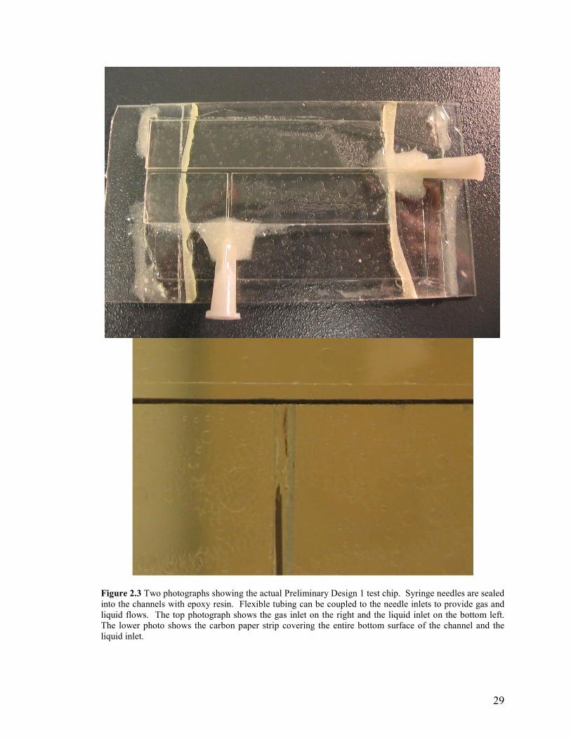
wall and seal the channel. .................................... 28 Figure 2.3 Two photographs showing the actual Preliminary Design 1 test chip. Syringe needles are sealed

into the channels with epoxy resin. Flexible tubing can be coupled to the needle inlets to provide gas

and liquid flows. The top photograph shows the gas inlet on the right and the liquid inlet on the

viii

bottom left. The lower photo shows the carbon paper strip covering the entire bottom surface of the

channel and the liquid inlet. ................................................................................................................ 29 Figure 2.4 Example of conventional visualization of droplet growth, emergence, and expulsion using

Preliminary Design 1. Gas velocity is on the order of 8x10-2

m/s, and is from right to left. .............. 30 Figure 2.5 Example plot of droplet height vs. time from a photograph series of a repeatable droplet

emergence and expulsion event similar to that shown in Figure 2.6, created using Preliminary Design

1. Gas velocity is about 0.083 m/s...................................................................................................... 30 Figure 2.6 The fabrication process for a 250-micron pore imbedded in a rectangular slab of PDMS with

square edges. (a) Make a mould using three 1mm-thick glass microscope slides stacked into a Petri

dish in a staggered fashion as shown. Attach a 250 micron diameter wire to the side surface of the

middle slide using a small dab of epoxy applied to the tip of the wire. Stretch the dab across the gap

so that it is narrow at the center. Secure the wire to the bottom slide with spacers and another dab of

epoxy. (b) Pour wet PDMS base mixed with curing agent into the mould. Cure the PDMS and allow

to set. (c) Cut the PDMS along the edge of the top glass slide and remove all excess from the mould,

leaving the PDMS slab sandwiched between the slides. (d) Pull the wire out of the PDMS slab,

breaking the epoxy dab and leaving a pore behind. (e) Pull the glass slides apart and remove the

PDMS slab with embedded 250 micron pore...................................................................................... 32 Figure 2.7 Two photographs showing the second chip design. The second photograph clearly shows the

250 micron pore and its intersection into the channel via the PDMS bottom wall of the channel. Flow

is injected into the pore via a syringe needle....................................................................................... 33 Figure 2.8 Several images of reciculating flow in a seeded water droplet being fed liquid from a 250 micron

pore in the center of the bottom wall of a 1mm square gas channel. The droplet is exposed to an air

flow from left to right of approximately 8x10-2

m/s. Illumination is provided by an arc lamp as

opposed to the laser. Images (a) and (b) show a droplet at the center of the channel at two different

stages of growth. Images (c) and (d) show the same droplet after it has wet the glass sidewall closest

to the observer. Particle streaks are clearer in (c) and (d) since the curved interface between the

droplet and the air has been eliminated due to this wetting................................................................. 34 Figure 2.9 Close-up sequence of particle flow patterns observed in a very large water droplet which is

about to block the entire channel. Gas flow is from right to left. Evidence of a strong clockwise

counter-rotation in the top right corner of (d) can be observed........................................................... 35 Figure 2.10 The completed test section with labeled components. 1: standard double-width glass

microscope slide. 2: cast rectangular polydimethylsiloxane (PDMS) strips 3 mm thick form top and

bottom channel walls. 3: flexible PDMS cover strip. 4: Toray PTFE treated carbon paper strip, 3

mm wide x ~ 300 microns thick. 5: syringe needle to couple gas flow from Tygon tube into channel.

6: PDMS sealant. 7: the gas channel, 1 mm high x 3 mm wide. ........................................................ 36 Figure 2.11 The test section. The flexible PDMS cover strip is being pulled back in order to allow access

to the channel so that a droplet may be pipetted onto the carbon paper surface.................................. 37 Figure 2.12 Cross sectional views of the two test section chip designs. Gas flow into the channel would be

directed into the page. ......................................................................................................................... 38 Figure 2.13 Sketch of droplet in an air flow (blue streamlines). Two cross sectional planes are illustrated.

The turquoise and green plane is the central plane of symmetry parallel to the x- and y- axes. The red

and yellow plane is a horizontal plane parallel to the x- and z- axes. The vectors in the planes are

sketched for illustrative purposes only and are not indicative of any real physical measurements. .... 40 Figure 2.14 Orientation of the droplet in the channel relative to the objective and the gas inlet. The carbon

paper surface is in the same plane as the page. The droplet is sitting on this surface. Drawing not to

scale..................................................................................................................................................... 42 Figure 2.15 Experimental apparatus. (1) Zeiss inverted microscope. (2) Cooled CCD camera. (3) Test

section set into the stage of the microscope, coupled to the air flow line. (4) Beam expander (black).

(5) Laser head. (6) Laser power supply and controller. (7) Bubbler humidifier. (8) Rotameter flow

meter and control valve. (9) Fluorescent lamp. ................................................................................... 44 Figure 2.16 Cross sectional view of the gas channel with droplet. m is the distance between the wall closest

to the microscope objective and the point on the droplet closest to the objective. k is the half-width of

the droplet. H is the height of the droplet. a is the central plane bisecting the droplet, parallel to the

field of view of the objective, and represented by the dotted line. Drawing not to scale. .................. 45 Figure 2.17 (a) Side view of a droplet sitting on the carbon paper surface of the gas channel in the test

section. This is what the microscope objective in Figs. 6 and 7 would see. (b) Side-view of a seeded

ix

droplet under quiescent conditions with camera exposure adjusted to brighten particles. (c) The same

droplet from (b) exposed to an air flow from right to left. The exposure has been set very long to

exaggerate the streak lines. The air velocity is not sufficient here to noticeably deform the droplet

shape. Image in (a) is not at the same scale as in (b) and (c)............................................................... 46 Figure 2.18 The left image shows a raw particle image of a droplet in the channel. The right image shows

the result of a mask drawn around the droplet. The blacked out area is not included in the micro-

DPIV processing calculations. ............................................................................................................ 51 Figure 3.1 (a) Example of raw particle image for mean air velocity of 2.2 m/s. (b) Vector field

corresponding to raw image. (c) Uncorrected vector field as imported into Matlab. Both axes are in

meters. (d) Vector field corrected for optical distortion, showing original vector field outline (thick

red line), and idealized droplet shape used for distortion correction (contour plot)............................ 58 Figure 3.2 (a) Example of raw particle image for mean air velocity of 4.2 m/s. (b) Vector field









red line), and idealized droplet shape used for distortion correction (contour plot)............................ 64 Figure 3.5 Maximum, minimum, and average peak velocity from each of the four sets of distortion-

corrected vector fields acquired. The error bars on the average peak velocity data points come from

the standard deviation of the peak velocity data at those air velocities. .............................................. 67 Figure 3.6 (a) Group A averaged u-component velocity profiles passing through the centre of rotation of

each droplet. Corrected vector fields in this group had heights ranging between 570 and 610 microns.

(b) Group B averaged u-component velocity profiles passing through the centre of rotation of each

droplet. Corrected vector fields in this group had heights ranging between 530 and 570 microns. ... 69 Figure 3.7 (a) Liquid u-Velocity vs. Air Velocity for group A at two specific y-positions from the carbon

paper surface, 138 microns and 512 microns. (b) Liquid u-Velocity vs. Air Velocity for group B at

two specific y-positions from the carbon paper surface, 140 microns and 510 microns. Liquid

velocity error bars come from the standard deviation of the subset of velocity profiles at each air flow

rate, at the given y-position. ................................................................................................................ 71 Figure 3.8 Physical distribution of the top 30% of the velocity vectors from all trials at each air flow rate.73 Figure 3.9 Physical distribution of the top 30% of the velocity vectors from the last 25 trials and the first 35

trials acquired for the air flow rate of 6.0 m/s. .................................................................................... 74 Figure A.1 The geometry of a droplet with a height H much greater than its contact line radius R, where H

= R + b.. A point P sitting on the surface of the droplet is defined in polar co-ordinates by radius r

polar angle θ, and azimuthal angle φ. The droplet profile in any r-θ plane (including the x-y plane) is

defined by the shape function ζ(θ). ..................................................................................................... 84 Figure A.2 Droplet height lost vs. time for the seven droplets used for this evaporation experiment. ......... 88 Figure A.3 Droplet volume lost vs. time for the seven droplets used for this evaporation experiment. ....... 89 Figure B.1 Chritical shedding air flow rate statistics for a 1 mm x 3 mm air flow channel with a GDL

sidewall. Droplet volume is 0.35 mm. Count percentage refers a percentage of the 50 trials acquired

for each chip. One count constitutes one observed shedding event.................................................... 92 Figure D.1 Radial and polar components of the normal vector shown in the plane φ = π/2, with respect to

the x- and y- axes indicated by the unit vectors i and j respectively. .................................................. 97 Figure D.2 Incident and refracted light beams A and B respectively, at the surface of the droplet. Vector B

is equal to the sum of vectors A and C. Vectors A, B, C and surface normal N all lie in plane S. .... 99 Figure D.3 Tracing a ray of light, depicted with red lines, as it passes between a point Po in the object plane

and a point Pi in the image plane....................................................................................................... 101 Figure D.4 Uncorrected micro-DPIV vector field from the center plane of a droplet in an air flow. Notice

that the x and y co-ordinate system has been centered at the middle of the droplet chord in order to

felicitate modelling of the droplet shape using the ideal model from Figure A.1. ............................ 104

x

Figure D.5 The corrected micro-DPIV vector field of Figure A8. The thick red curve shows the original

droplet boundary drawn by the Matlab program around the un-masked portion of the un-corrected

vector field. The contour plot represents the idealized 3-D droplet surface defining zs(x, y) used to

perform the correction. The corrected vector field has been truncated so that it only extends outwards

from the origin to 80% of the radius r of the shape, where the radius of the shape is defined as in

Figure A.1. ........................................................................................................................................ 106 Figure D.6 (a) Computer simulation of a regular grid bisecting an idealized water droplet. The grid lines

are distorted due to the refraction of the light passing through the interface of the droplet and the air.

(b) The same image after processing by a distortion correction algorithm. Notice that the original

grid can only be restored within about eighty percent of the radius of the droplet, due to the loss of

information around the far edge of the droplet from the distortion in (a). ........................................ 107 Figure E.1 Original raw PIV image example.............................................................................................. 114 Figure E.2 Colour-inverted image mirrored along the contact line in order to simulate a reflection. ........ 114 Figure E.3 Colour-inverted image mirrored along the contact line in order to simulate a reflection. ........ 116 Figure F.1 A droplet sitting on the carbon paper surface of the channel in the top view chip. The focal

plane has been aligned with the carbon paper surface as a as a y-axis zero reference point. ............ 117 Figure F.2 A droplet sitting on the carbon paper surface of the channel in the top view chip. The focal

plane has been advanced 0.35 mm in the posititive y-direction to focus on the approximate vertical

center plane of the droplet. ................................................................................................................ 118 Figure F.3 A raw particle image from the droplet in Figures A14 and A15. .............................................. 119 Figure F.4 The vector result from 30 pairs of raw images similar to that shown in Figure A18. ............... 119

xi

List of Tables Table 2.1 Air flow rates used in this experiment and corresponding ∆t settings in the DaVis PIV software.

............................................................................................................................................................. 48 Table 2.2 Number of trials acquired and ∆t setting used for each flow rate number. ................................. 50 Table 3.1 Average droplet dimensions and estimated volume...................................................................... 65 Table 3.2 Results from contact angle measurements performed on the droplet image sub-samples. ........... 66 Table 3.3 Raw data from Figure 3.5. ............................................................................................................ 67 Table A.1 Measurements of R, b, and k from an actual droplet photograph, and the droplet volume

approximation results from equation (A8) compared to the perfect sphere assumption. .................... 86 Table A.2 Droplet position q and approximated starting volume. ................................................................ 87 Table B.1 Droplet position and size statistics. .............................................................................................. 92 Table C.1 Correlation table for Omega FL-3804G for dry air at 23°°°°C......................................................... 95

xii

Acknowledgements

First, I would like to extend my sincere thanks to my supervisors, Dr. Peter Oshkai and

Dr. Ned Djilali, for their unending guidance during the course of my Masters project at

UVic. This work simply would not have been possible without their technical, financial,

and emotional support.

Second, I would like to thank Dr. David Sinton, who was not one of my official

supervisors, but could easily have acted as one. The learning experiences I gained by

working with his microfluidics group, and the laboratory resources made available to me

by him were absolutely invaluable to my project.

Third, I would like to acknowledge the generous financial support provided for this

project by Ballard Power Systems Inc., Canada Research Chairs, NSERC, and Western

Economic Development Canada.

xiii

Dedication

For all my friends and family who helped me get to this point in one piece.

Chapter 1 Introduction

1.1 Background and Motivation

Proton exchange membrane fuel cells (PEMFC’s) together with hydrogen have

the potential to significantly reduce our dependence on fossil fuels for transportation.

However, their successful commercial implementation is contingent on the demonstration

of an automotive fuel cell system that is both technically and economically competitive

with current internal combustion technologies. Fuel cell operating efficiencies must be

improved [1]. Water management and two-phase flow in fuel cell gas channels are major

areas of concern. The following background literature review will highlight the

importance of water management in PEMFC’s, and then examines some experimental,

analytical, and numerical works done to date that relate to the visualization, modeling,

and analysis of water accumulation and two-phase flows in PEMFC flow channels.

1.1.1 Water Management in PEM Fuel Cells

A schematic of the operation of a PEMFC is shown in Figure 1.1. Reactant gases

are pumped through flow channels that recess into two electrically conductive ‘bipolar’

plates. Oxygen (or air) is pumped through the flow channels in the cathode plate, and

hydrogen is pumped through the channels in the anode plate. These plates sandwich the

membrane-electrode assembly (MEA).

2

Figure 1.1 (a) Cross sectional view of a PEMFC parallel to gas flow channels, showing the arrangement of

the primary fuel cell components. Depending on the gas channel orientation in the bipolar plates, flow may

move into or out of the page as denoted by the arrows. (b) Cross sectional view perpendicular to gas flow

channels as denoted by Section A in (a). Reactant flows and electrochemical reactions are labeled [2]. The

relative sizes of the bipolar plates, membrane, catalyst layers and GDLs are not to scale.

3

The MEA consists of the assembly of a polymeric proton exchange membrane,

catalyst layers and gas diffusions layers (GDLs) as shown in Figure 1.1(a). The

membrane is coated on each side with a thin catalyst layer and then sandwiched between

the porous anode and cathode gas diffusion layer electrodes (anode and cathode GDL

respectively), which are both electrically conductive.. The bipolar plates contact the

GDL electrodes at the land area, shown in Figure 1.1 (a).

Hydrogen gas diffuses from the anode flow channel through the anode GDL and

dissociates into two protons and two electrons at the anode-side catalyst layer of the

membrane. The electrons are conducted from the anode layer through the load and into

the cathode layer, while the protons pass through the membrane itself. At the cathode

catalyst layer, the protons combine with oxygen that has diffused through the cathode

GDL from the cathode flow channel, and electrons that have passed through the load.

This produces water in the cathode GDL [2].

The proton conductivity of the membrane is highly dependent on its level of

hydration. The result of electro-osmotic drag within the membrane and electrochemical

water formation at the cathode is a net accumulation of excess water at the cathode side

of the MEA, and dehydration at the anode side. Back diffusion from the cathode to the

anode due to the water concentration gradient has been shown to be insufficient for

keeping the anode side hydrated at high current densities [2]. Moreover, if water content

throughout the MEA increases to sufficiently high levels, then the cathode GDL floods

and liquid water accumulation in the form of droplets can occur in the cathode gas

channels.

4

Figure 1.2 below is taken from an experiment by Wang et al. and shows a

sequence of photographs looking through the top of transparent PEMFC cathode gas

channel onto the GDL surface. Between 0 and 180 seconds two discrete water droplets

that have formed in the channel on the GDL can be seen growing continuously. By 480

seconds the droplets have grown to the point where their surfaces have contacted, causing

them to merge and then coalesce with the more hydrophilic channel sidewall. Between

480 and 540 seconds the drop on the sidewall is expelled in an annular flow regime and a

new droplet begins to form close to the same preferential locations as the first two.

Figure 1.2 Top-view snapshots of the dynamic process of water droplet formation and expulsion in a

transparent PEMFC gas channel at 0.82 A/cm2 and 70°C [3].

Under certain operating conditions, water droplets forming in the gas channels

may bridge between the walls of the channels, causing partial or complete gas flow

5

blockage. A photograph of a complete gas flow channel blockage is show in Figure 1.3

[3].

Figure 1.3 A gas flow channel completely blocked by a water plug [3].

Such blockages can significantly affect cell performance, as reactant supply to the

membrane is then partially or entirely inhibited [4]. Tüber et al. performed an experiment

with a fuel cell having a simple bipolar plates with two gas channels [5]. A current

density plot in time for this fuel cell operating in constant voltage discharge mode under

3 different gas flow rate conditions was generated. It was observed that if the gas flow

rate was not sufficient to keep droplets out of the channels either by evaporation or forced

convection, a blockage occurred, causing a 25% slump in current density.

Due to the intricate balance of conditions that must be maintained during fuel cell

operation, removing liquid water droplets from gas flow channels to improve

performance is not a simple matter of increasing the temperature in the gas channels or

increasing the gas flow [6].

6

1.1.2 Droplet Behaviour in Gas Transport Channels

An increased understanding of the fluid dynamics and interaction between two-

phase droplet-and-air flows in gas transport channels at the fundamental level may help

in the development of mechanisms for droplet removal, and may also provide crucial

validation for numerical simulations of such droplet flows. A growing body of

experimental, computational, and analytical work devoted to this study has already

highlighted some of the fundamental issues. Some attention has been drawn specifically

to single droplet removal from porous hydrophobic surfaces in such channels by air flow.

Notable experimental works by Kumbur et al. [7] and Theodorakakos et al. [8]

concentrate on the relationship between gas flow rates, the degree of droplet deformation

characterized by contact angle hysteresis, and the force balance acting on the droplet [7,

8]. Although these works have set a solid foundation in the field, they are certainly not

comprehensive. There is still a lack of empirical information available about the details

of the interaction between the air and liquid phases during droplet shedding from GDL-

type surfaces. The most significant works will be reviewed here, and potential areas for

future study will be highlighted.

7

Figure 1.4 Water droplet emergence into a cathode gas channel [9].

It has been observed by a number of authors in the literature that water emerges

through the surface of the GDL into the cathode gas flow channels in an eruptive process

and forms discrete droplets, as shown in Figure 1.4. Air is forced to flow around these

droplets, sometimes creating substantial pressure drops across the gas channels. The

exact mechanisms inside the GDL that trigger water eruption are not completely known,

but the event is intimately tied to GDL structure and the operating conditions of the fuel

cell. In some cases water will emerge away from the land area near the center of the gas

flow channels, while in other cases it will emerge closer to the channel sidewalls, or even

in contact with them [6]. Water emergence from the GDL is a field of study within itself,

and is beyond the scope of this work.

droplet

8

Clearly, there are countless permutations of the physical orientation of the droplet

inside the channel in such flows. In order to simplify this review, the scope will be

narrowed to include only the case of a single droplet sitting at the center of the GDL

surface of a PEMFC cathode flow channel, not adhered to any side walls, and exposed to

an air flow as shown in Figure 1.4. Additionally, depending on the interaction between

the preferential pathways for liquid flow inside the GDL pore network, and the rate of

liquid water production, the droplet may grow to a certain fixed volume, continue to

grow, or actually shrink in size, in some cases shrinking while a neighbouring droplet

begins to grow [9, 10]. This thesis will consider both static and dynamic shapes and

volumes for single droplets, but the main focus will be static shapes.

Once a droplet begins to emerge into the channel, it will be exposed to shear and

pressure forces from the air flow. The droplet will deform as a result of these forces and

exhibit a contact angle hysteresis ∆, defined as the difference between the advancing and

receding contact angles, θA and θR respectively, as illustrated in Figure 1.5 (a). If the

shear and pressure forces are stronger that the interfacial forces that pin the droplet to the

GDL, the droplet will shed from the surface and advance down the channel in the

direction of the air flow.

9

Figure 1.5 Sketch of 2-dimensional cross-section of a water droplet sitting on a surface in a small gas

channel exposed to an air flow moving right to left. (a) The droplet is deforming due to the air flow. The

downstream contact angle θA is termed the advancing contact angle, whereas the upstream contact angle θR

is termed the receding contact angle. Droplet height H and chord length c are shown. (b) Shear (FShear),

pressure (FP), and drag (FDrag) forces acting on the control volume A’ABB’ drawn in the channel over the

droplet. The surface tension force (Fst) acts to pin the droplet to the bottom surface. The x-component

velocity profile for the simplified parallel-plate Poiseuille flow assumption made by Kumbur et al. is shown

over the smaller rectangle A’A”B”B’ drawn around the droplet. (c) A more realistic sketch of the expected

velocity profile for the same droplet. The shear from the air flow induces a secondary rotational flow

inside the droplet, shown by the streamlines. The velocity at the interface of the liquid and air phases is

non-zero.

A recent experimental and analytical study by Kumbur, Sharp, and Mench

focuses specifically on this droplet-in-air-flow force balance [7]. In this work, an

equation for the force balance on a static droplet is achieved by considering the horizontal

components of the pressure force (FP), drag force (FDrag), and shear force (FShear) acting

on a rectangular control volume drawn around the droplet in the channel, shown as

rectangle A’ABB’ in Figure 1.5 (b). The sum of these forces is equated to zero using

Newton’s second law.

The horizontal component of the drag force is solved, and then balanced with the

horizontal component of the interfacial surface tension force (Fst) that pins the droplet to

the GDL. This force balance is represented by the following inequality [7]

10

)(xShearxPDragst xx

FFFF +−=≥ (1)

This inequality is the condition for droplet stability. If the drag force on the droplet from

the air flow exceeds the surface tension force, then the droplet will shed on the GDL

surface and move down the channel in the direction of the air flow. Kumbur et al do not

determine the drag force explicitly. Rather, analytical expressions for the x-components

of Fst, FP and FShear are obtained and substituted into (1) to form an equation containing

engineering parameters, including average channel velocity U, contact angle hysteresis ∆,

advancing contact angle θA, air viscosity, channel and droplet geometry, and surface

tension. FDrag is found implicitly from FP and FShear.

The treatment of the air phase model for flow around the droplet is critical in

determining correct analytical expressions for these forces. In their approach, Kumbur et

al. [7] model the air flowing over the droplet as a simplified Poiseuille pressure driven

flow between two infinite parallel plates within the rectangle A”ABB” sketched in Figure

1.5 (b). Although the force balance model derived from this treatment is an excellent

first attempt and does show some agreement with experimental data, the simplified

approach sheds little light on the actual interaction between the air and liquid phases.

Intuitively, one can guess that the shear forces from the air flow induce a

secondary flow in the liquid phase inside the droplet, as sketched in Figure 1.5 (c). Thus,

the fluid motion at the droplet surface is non-zero and perhaps quite significant. In

addition, the deformation of the droplet due to the flow, characterized by the advancing

and receding contact angles shown in Figure 1.5 (a), creates an asymmetry in the flow

field upstream and downstream from the droplet. These factors both cause the drag and

pressure forces acting on a real droplet to deviate substantially from those seen by a

11

rectangular box, or for that matter a rigid droplet. Moreover, Horton (1965) points out

that several previous works dating back as far as 1959 have demonstrated that the drag

coefficient for a fluid sphere is considerably lower than that of an equivalent rigid sphere

moving in the same medium [11].

A 5 mm x 4 mm channel gas channel model was built by Kumbur et al. [7] with

aluminium sidewalls and a Lexan ceiling in order to perform experiments for validation

of the analytical model. The bottom wall is a carbon paper GDL with varying degrees of

PTFE treatment. Liquid is pumped through the GDL into the channel to create droplets

on the surface of the GDL. Air is pumped through the gas channel in order to simulate

PEMFC operation. Several measurements are made on this system and compared to

results predicted by the force balance model. First, scatter plots of contact angle

hysteresis vs. droplet height-to-chord-length aspect ratio were generated for a range of

Reynolds numbers, where Reynolds number is calculated using average channel air

velocity and channel hydraulic diameter. From these scatter plots, a functionality is

obtained relating contact angle hysteresis to Reynolds number, height, and chord length.

This functionality was then incorporated into the force balance model to obtain a

relationship between droplet aspect ratio (height to chord length) and Reynolds number at

the onset of droplet separation from the GDL. A plot comparing experimental

measurements of stable droplets with certain aspect ratios at a variety of Reynolds

numbers is obtained and compared to the force balance curve. This plot is shown in

Figure 1.6.

12

Figure 1.6 Relationship between Reynolds number and droplet aspect ratio at the onset of droplet shedding

from the GDL surface, as predicted by the force balance model developed in [7]. Experimental

measurements from stable droplets are plotted using the small triangles. Note that the curve tends to

underpredict droplet stability at low Reynolds numbers, and overpredict it at high Reynolds numbers.

81% of the measured points from the experiment performed by Kumbur et al. fall

into the predicted stable zone. Of particular note is that their model tends to underpredict

droplet stability at lower air-phase Reynolds numbers below approximately 700, and

overpredict stability at higher Reynolds above 700. A detachment test was also

performed, with all points landing in the predicted detachment zone. Droplet chord

length is 2.3 mm. Air flow Reynolds number varied from 0 to 1800. PTFE

concentrations used were 5 and 20%.

Chen, et al. [12] performed a concurrent, independent, and nearly identical study

to Kumbur et al. Again, they built a force balance model for a droplet in an channel air

13

flow using a control volume approach, and predicted droplet instability by balancing the

surface tension force pinning the droplet to the GDL with the shear and pressure forces

fighting to remove the droplet from the surface. The treatment of the force expressions

differs somewhat between the two works, but the simplifying assumption of fully

developed flow between two parallel plates over the top of the droplet is notably the

same. Like the work of Kumbur et al., a plot of the critical droplet height in the channel

vs. the contact angle hysteresis predicted by the model is generated to show a divide

between unstable and stable droplet regions. An experiment is constructed to generate

water droplets by pumping water through a GDL into a channel with humidified air flow,

allowing photographic visualization from a side view. Snapshots of droplets in various

stages of growth before detachment are taken. Droplet height and contact angle

hysteresis are recorded from these snapshots, and plotted on the stability map described

above. An example plot from the work is shown in Figure 1.7.

The force balance model developed by Chen et al. consistently overpredicts

droplet stability at flow rates of about 0.4 m/s and higher, as demonstrated by the gap

between experimental data and the theoretical stability threshold indicated in Figure 1.7.

It is suspected in the work that this is due to the over-simplified treatment of the air phase

flow.

14

Figure 1.7 Theoretically predicted droplet stability zone from Chen’s force balance model for two different

flow rates, compared to experimental measurements of stable droplets. Note that the force balance model

consistently overpredicts droplet stability for the higher flow rate [12].

Theodorakakos et al. performed an investigation into a similar droplet flow

scenario, combining computational work with experimental validation [8]. In their paper,

a force balance on a droplet in a gas channel is discussed. The critical air flow rate

sufficient to initiate droplet movement on the GDL is said to correspond to the critical

advancing and receding contact angles of the droplet when deformed by the air flow, as

well as a critical droplet diameter. An experimental gas channel of dimensions 2.7 mm x

7 mm with a GDL surface made from carbon paper was built to simulate the droplet

shedding event, into which droplets were placed via a pipette. The advancing and

receding contact angles that occur just before droplet movement were recorded via digital

photography, along with the droplet diameter. In house CFD software was then used to

reproduce the experiment numerically, which incorporated equations developed in the

15

force balance model. The software applies the Volume of Fluid (VOF) method to track

the liquid and gas phases. The critical advancing and receding contact angles for droplet

shedding, which were derived from the experiments, were set in the code. The calculated

droplet diameter corresponding to the shedding event is then extracted from the

numerical simulations and compared to the experimentally measured diameters for the

same flow conditions. Air velocity in both the numerical and experimental cases is

varied between 4 and 16 m/s. Droplet diameter is varied between 0.4 and 2 mm. Good

agreement was found between experiment and numerical study, suggesting that the VOF

method is indeed useful for simulating droplet shedding events. However, the study

failed to go into the details of the air and liquid phase interaction at the interface, which is

not only critical to the understanding of the dynamics, but also presents another avenue

for validation of numerical approaches.

16

1.2 Micro-DPIV Fundamentals

Digital particle image velocimetry (DPIV) is a fluid flow visualization and

velocity measurement technique that can be applied to a broad range of flow scenarios, as

described by Westerwheel (1997) and Sinton (2004) [13, 14]. Micro-DPIV is the micro-

scale complement to macro-DPIV. Both techniques are based on tracking the motion of

illuminated tracer particles in the fluid via digital photography.

The main steps of DPIV using cross-correlation are illustrated in Figure 1.8. In

conventional macro-DPIV, a plane of reflective particles in the flow is illuminated,

usually by means of a laser sheet. During the measurement procedure, the laser fires

twice with a known time difference ∆t between firings. A digital camera, which is timed

with the laser, acquires a pair of images of the illuminated particles separated by ∆t.

Within ∆t the particles in the image plane will have displaced a small amount based on

the velocity of the fluid in the immediate vicinity of each of the particles. PIV processing

software will divide these two sequential particle images into equally sized interrogation

zones of X by X pixels. Two corresponding interrogation zones, one from each image in

the pair, are cross-correlated using a software algorithm to obtain a displacement vector,

from which a velocity vector can be inferred using the known ∆t. One velocity vector is

assigned in this way to each interrogation zone to produce a complete velocity field for

the flow. Laser light is used in DPIV primarily because of its sharply defined

wavelength, which allows background light of different wavelengths to be easily filtered

out during image capture.

17

Figure 1.8 Digital particle image velocimetry using cross-correlation [15].

In micro-DPIV applications, the characteristic length scales of the flow systems

being measured generally approach the thickness of a typical laser sheet, and in many

cases the alignment of sheet optics with a small-scale, complex apparatus can become an

arduous task. Thus, volume illumination is used instead, often by means of a laser beam

passing through a beam expander. All tracer particles in the test section are thus

illuminated. Image planes in the flow are acquired by relying on the focal properties of

microscope optics. Consequently, a lower particle seeding density must be used to

reduce noise from out-of-plane particles, and there is also some unavoidable depth-based

volume averaging of the flow field.

18

The diameter of micro-DPIV particles is on the same order as the wavelength of

the laser light used, and the physics of light scattering changes at that limit. Fluorescent

particles are used instead of reflective ones, which absorb the laser light rather than

scatter it, and emit light of a different wavelength after an energy shift [15]. A filter is

often used to pass only light of the latter wavelength to the camera, thus further helping

to eliminate unwanted noise and reflections from the incident light.

1.3 Research Objectives

It is clear from the literature that there is a need for further investigation into the

underlying physics behind the interaction between the air and liquid phases in such

droplet-in-air-flow scenarios. In particular, the three primary experimental works

discussed above by Kumbur et al., Chen et al., and Theodorakakos et al. all neglect to

illustrate the secondary swirling motion induced inside the liquid droplet due to shear

from the air flow, while Kumbur et al. and Chen et al. neglect to incorporate the effects of

this motion into their force balance models at all. Again, much older experimental

studies point towards the significance of these secondary effects on the forces

experienced by the droplets [11].

The experimental project around which this thesis is based was designed to

improve understanding in this area with the following goals in mind:

Develop a method for applying 2-D micro-digital-particle-image-velocimetry (micro-

DPIV) techniques towards the qualitative and quantitative visualization of the secondary

flows induced inside the liquid phase for the case of air flow around a droplet adhered to

the porous bottom wall of a PEMFC gas channel model.

19

Acquire a relevant set of data from the experimental technique that could be

compared to results from a computational simulation of the same flow scenario.

Investigate and/or suggest further avenues of study possible by using or modifying

the methods developed for the experiment, including an improved force balance model.

Micro-DPIV was chosen for this experiment because of its reputation as a pre-

eminent technique in micro-scale flow analysis. Resolution and accuracy for micro-

DPIV derived velocity fields are said to be superior to other particle based velocity field

measurement techniques, including Laser Doppler Velocimetry (LDV), which provides

less information per interrogation window than DPIV [14].

20

Chapter 2 Experimental System and Techniques

2.1 The Micro-DPIV System and Flow Apparatus

Figure 2.1 Apparatus used in this experiment. The internal microscope workings are taken from the

LaVision DaVis micro-PIV manual. 1: Nd:YAG laser head. 2: beam expander. 3: Hg vapour lamp. 4:

New Wave Solo PIV ™ laser power supply. 5: test section with droplet. 6: green ~542 nm light from

laser (up arrow). 7: red ~ 612 nm light from fluorescent microspheres (down arrow). 8: microscope

objective, high NA. 9: filter cube with epi-fluorescent prism. 10: beam splitter. 11: ocular. 12: relay lens.

13: cooled CCD camera. 14: computer with LaVision DaVis ™ PIV software suite. 15: wall regulator and

valve to dry air supply. 16: direction of air flow. 17: check valve. 18: ball rotameter flowmeter w/ flow

control valve. 19: bubbler humidifier. Components 3, 8, 9, 10, 11, and 12 are all part of a Zeiss Axiovert

200 inverted microscope.

The apparatus used in this experiment is shown in detail in Figure 2.1. The test

section (item 5) consists of a straight, optically accessible, rectangular gas channel into

21

which a droplet seeded with tracer particles is placed. The test section will be discussed

in further detail later. Dry air from the wall regulator (item 15) passes through a

rotameter flowmeter (item 18), a humidifier (item 19), and into the test section in order to

reproduce the scenario inside the channel sketched in Figure 1.5 (a). The flowmeter has a

range between 0 and 2.3 L/min, and a valve for controlling the flow rate. The humidifier

allows the dry air to bubble through a water column approximately 7 cm high. The

purpose of the humidifier is simply to curb evaporation and extend the lifetime of a

droplet placed in the test section. Preliminary tests performed prior to the actual PIV

experiment, to be discussed in subsequent sections, showed that the humidifier helps to

extend the droplet lifetime in the channel by a factor of about seven. The Zeiss Axiovert

200 inverted microscope with a Zeiss 5x EC Plan-Neofluar objective was used to view

the test section. A Nd:YAG laser head (item 1) fires green light pulses with a wavelength

of approximately ~ 542 nm, which pass through the beam expander and microscope

optics and fall incident on the test section.

The tracer particles used in this experiment are polystyrene microspheres with a

diameter of 1 micron, purchased from Duke Scientific, which are dyed throughout with a

red fluorescent dye that has absorption and emission peaks at 542 nm (green) and 612 nm

(red) respectively. An epi-fluorescent cube inside the microscope housing filters out any

green light reflected from the test section and passes only the red light to the cooled CCD

camera (item 13). This camera captures the images of the particles with a resolution of

1024 by 1376 pixels, and sends them to a computer (item 14) for processing.

The depth of field is the distance along the optical axis of the microscope in the

object plane in which items will appear to be in focus in the image plane. This distance is

22

important since it represents the volume averaging depth for in-focus particles using the

micro-DPIV method. The microscope objective has a depth of field that can be

approximated using the following equation [16]

,NAMNA

dd

2

d0tot e

nnd

⋅+=

λ (2)

λ0 is the wavelength of the light magnified by the objective, which is 612 nm for the red

light emitted by the tracer particles. nd is the index of refraction of the medium in which

the focal plane lies. Although the light must pass through both water and air in the case

of this experiment, the index of refraction of water, 1.33, will be used, since it is slightly

larger than that of air and will provide a coarser, more conservative estimate for the depth

of field. M is the degree of magnification of the objective, which is 5x in the case of this

experiment. ed is the smallest distance resolved by a detector placed in the image plane

of the microscope objective. In this experiment, the detector is the charge coupled device

(CCD) of the digital camera used to capture the light from the particles. This CCD

translates the captured light into a 1024 x 1376 pixel digital photograph with a pixel

dimension of approximately 9.97x10-7

m/pixel at 5x magnification. This pixel length

scale will be used as the smallest resolvable distance in the depth of field calculation.

NA is the numerical aperture of the lens, which is 0.16 for the Zeiss 5x EC Plan Neofluar.

Using these parameter values, the calculated value for depth of field dtot is approximately

34 microns. Thus, all tracer particles falling within the 34 micron depth of field will

contribute to the depth-averaged velocity measurement.

The Stokes number of a particle, given by

c

o

d

USt

τ= , (3)

23

is a dimensionless number that quantifies the ability of a tracer particle to follow the

streamlines of a flowing fluid [17, 18]. Particles having St << 1 will follow the flow very

well, whereas particles having St >> 1 will not follow the flow at all. Here, τ is the

relaxation time equal to βσ2/18ν, where β is the particle to fluid density ratio, σ is the

tracer particle diameter equal to 1 micron, and ν is the kinematic viscosity for deionized

water at 20°C equal to 1.004 x 10-6

m2/s [19]. The density of the polystyrene spheres is

1060 kg/m3, whereas the density of deinonized water at room temperature is 998 kg/m

3.

Thus β ≈ 1.06. Uo is the flow velocity in the fluid, assumed to be 0.1 m/s, which is on

the same order as the maximum flow velocity measured thus far. dc is the characteristic

dimension, which is assumed to be the mean width of a water droplet, or 770 microns.

Thus we have a Stokes number of 1.2 x 10-5

, which indicates that the polystyrene

particles follow the water flow very well and are a good choice as a tracer particle for this

application.

During this experiment, the PIV sum-of-correlation method was used in the

LaVision DaVis software package to calculate the vector fields. The sum-of-correlation

method, to be outlined in greater detail in later sections, is an averaging technique that is

used when individual PIV image pairs from a flow produce vector fields with a large

proportion of bad vector regions due to low seeding density, high image noise, poor

particle visibility, or high out-of-plane particle noise, which are all factors present in this

experiment. In this case, for each velocity field measurement, 30 consecutive image pairs

of the steady-state flow were acquired at approximately 5 pairs per second. To perform

the sum-of-correlation method on these 30 images, DaVis cross-correlates each pair of

interrogation zones for the 30 image pairs and then adds the results from each. A single

24

displacement vector for each interrogation zone is then acquired from the sum of the

cross-correlation results [15].

2.2 Channel Model Design and Fabrication

The design and fabrication of the test section, shown as item 5 in Figure 2.1, which

contains the model for the PEMFC gas channel to be used in the experiment, formed a

crucial component of this project. The test section had to conform to the following

design constraints:

(a) It had to be built in the format of a conveniently sized, transportable chip that

would fit into the stage of the Zeiss inverted microscope.

(b) It had to be optically accessible (transparent).

(c) It had to contain a model of a straight, rectangular PEMFC gas channel with three

smooth sidewalls and a forth sidewall composed of a porous GDL surface, and of

a sufficient length to allow fully developed flow in the air phase downstream

from the air inlet.

(d) It had to permit a side view or top view of the interior of the gas channel with

respect to the microscope stage.

(e) It had to have a sealed air inlet for the gas channel that can be easily coupled to a

pressurized air system to provide an air flow.

(f) It had to incorporate a system to permit the introduction of water droplets of a

reasonably repeatable size onto the GDL surface in the channel, at a reasonably

repeatable position near or about the center of the channel, which would not touch

the other sidewalls.

25

(g) It had to be manufactured in a cheap and repeatable manner, so that many clean

copies of the test section could be reproduced to avoid the effects of material

degradation, dust contamination, and pollution with fluorescent polystyrene

spheres.

The dimensions of the gas channel were not constrained at the beginning of the design

phase, since these could be tuned to suit either the type of flow measurement desired, or

additional constraints imposed on the design due to the choice of fabrication technique.

2.2.1 Working Materials and Fabrication Techniques

A variety of fabrication methods had to be reviewed in order to choose a method

for building a device to meet the design constraints listed above. After the review, it was

decided that the techniques commonly used for manufacturing microfluidic devices

would be best suited to this purpose. Microfluidic devices take advantage of the changes

in the dominant governing force terms that arise in fluid flow systems operating in very

low Reynolds numbers regimes in order perform a wide range of tasks. These dominant

force term changes often occur when the characteristic length scale of a flow system

moves into the micro-range. Fields of application for microfluidic devices include

membraneless bio-fuel cells, and on-chip systems for chemical and biological analysis

[20].

Microfluidic devices of a variety of sorts are commonly made out of a transparent,

flexible organic polymer called polydimethylsiloxane, or PDMS, which has the chemical

formula (H3C)[SiO(CH3)2]nSi(CH3)3. This elastomer base is often supplied commercially

in a viscous liquid state at room temperature. It can be mixed with a curing agent, which

26

introduces cross-links that solidify the base into a rubbery, transparent material that

bonds very well to glass via reversible van der Walls forces. Cured PDMS is optically

transparent down to 280 nm, which makes it ideal for supporting a variety of

fluorescence-based flow visualization techniques. This curing process can be performed

within a range of temperatures in order to tune the mechanical and surface properties of

the thermoset. PDMS is easily molded, taking the shape of its surroundings extremely

well. It is often used to reproduce networks of microscopic flow channels having

characteristic length scales on the order of 50 microns, accurately capturing the details of

the surface imperfections in the master, which may be on the order of microns or less.

The surface of PDMS that is cured while mated to a smooth piece of glass is generally

hydrophobic, but does not have the same degree of hydrophobicity as a 40 % wt. PTFE

treated carbon paper due to the higher degree of surface roughness intrinsic to the carbon

paper, which contributes to instability at the three phase line. PDMS can be semi-cured

into a very viscous, tacky, glue-like state that can be used to seal seams and bond pieces

of glass and PDMS together. Further curing of this semi-cured PDMS will result in a

tight, rigid seal.

Additionally, PDMS has the advantage of being much cheaper than glass or

silicon, and the casting and curing technique used for forming PDMS components is

simpler and less expensive than, for example, the micro-machining of Plexiglas, or clean

room fabrication of silicon, which often includes ion etching or chemical wet-etching.

This allows PDMS-based device structures to be fabricated in-lab in large, repeatable

quantities, without relying on time-consuming and expensive outsourcing. By exercising

27

some creativity in manufacturing, PDMS can be used to create almost any micro-scale

structure, and so it was seen to be ideally suited for the purposes of this project.

2.2.2 Preliminary Design Iterations and Results

The scope of this experimental project was not intuitively obvious during its

initial stages. As a result, several different attempts were made to produce a useful test

section, with slightly loftier goals than those actually settled on in the end. Initially, the

idea was to produce a test section that would allow water to be pumped through the GDL

side wall, simulating the growth of actual water droplets on the surface of the GDL

during fuel cell operation. Out of a number of failed trial-and-error design approaches in

the lab, two particular designs actually produced interesting visualizations that could be

pursued as extrapolations to the current project. These designs will be discussed briefly

in this section.

2.2.2.1 Preliminary Design 1: Epoxy-Sealed 1mm Square Glass Channel

The first preliminary design is a 1mm x 1mm square gas transport channel with a

PTFE-treated carbon paper bottom wall. The sidewall through which the microscope

objective looks is made from glass, the ceiling is made from glass, and the opposite

sidewall is made from PDMS. A liquid flow channel of dimensions approximately

similar to the 1mm x 1mm gas channel intersects the gas channel to form a T-junction.

The carbon paper covers the liquid inlet at this junction and all four seams at the junction

are sealed. The fabrication process used to make this chip is summarized in Figure 2.2.

Photographs of the completed chip are provided in Figure 2.3.

28

Figure 2.2 The manufacturing process for Preliminary Chip Design 1. (a) Begin with a clean, 1 mm thick,

double-wide glass microscope slide. Spin-coat one surface of this slide with a layer of semi-cured liquid

PDMS. (b) Cut another double-wide glass slide into three pieces. Align the smooth un-cut edges on the

first slide to make a T-juncion and set them into the wet PDMS. 1.3 mm o.d. brass rods to space these

pieces. (c) Fully cure the PDMS, then remove the brass rods and cut out the PDMS that has set in between

the cut pieces. (d) Using epoxy, affix a 300-micron-thick carbon paper strip to lower-inside surface of the

top of the “T” such that it covers the junction. (e) Spread epoxy onto the three seams created at the

junction. (f) Place another glass slide coated with semi-cured tacky PDMS over the junction and cure to

create the 4th

wall and seal the channel.

29

Figure 2.3 Two photographs showing the actual Preliminary Design 1 test chip. Syringe needles are sealed

into the channels with epoxy resin. Flexible tubing can be coupled to the needle inlets to provide gas and

liquid flows. The top photograph shows the gas inlet on the right and the liquid inlet on the bottom left.

The lower photo shows the carbon paper strip covering the entire bottom surface of the channel and the

liquid inlet.

30

Figure 2.4 Example of conventional visualization of droplet growth, emergence, and expulsion using

Preliminary Design 1. Gas velocity is on the order of 8x10-2

m/s, and is from right to left.

Figure 2.5 Example plot of droplet height vs. time from a photograph series of a repeatable droplet

emergence and expulsion event similar to that shown in Figure 2.6, created using Preliminary Design 1.

Gas velocity is about 0.083 m/s.

31

Figure 2.4 shows a series of photographs taken by the inverted microscope

looking though the bottom glass slide into the channel, while liquid water is being

pumped though the carbon paper into the channel at the T-junction using a syringe pump.

Gas is being pumped from right to left by another syringe pump. The water droplet in

this case is expelled after it completely fills the channel and blocks air flow. Depending

on the air and liquid flow rates set, droplet emergence and expulsion in this manner can

be made into a reasonably repeatable event.

Sets of photographs of droplet emergence and expulsion events created using

Preliminary Design 1, taken at 3 Hz, were acquired for a variety of flow rate

combinations. Using an edge detection algorithm in Matlab to analyze these droplet

photos, the height of the droplet can be plotted in time. An example plot is shown in

Figure 2.5, where the event seems to have a period of about 11-12 seconds.

2.2.2.2 Preliminary Design 2: Sealed 1mm PDMS Channel With Micro-

pore

The second successful chip was designed with a different experimental approach

in mind. Instead of having a liquid inlet covered by a strip of carbon paper, a small pore

with a diameter of 250 microns was cast directly into a PDMS bottom wall. Thus, a

single droplet can be introduced into the channel by injecting water through this pore.

This chip was built on top of a glass microscope substrate as with Preliminary Design 1.

However, the top and bottom walls and cover strip were constructed out of 1mm-thick

cast slabs of PDMS instead of glass microscope slides. The casting procedure for the

bottom wall slab with the imbedded 250 micron pore is outlined in Figure 2.6. The

32

completed channel with a close up of the pore inlet to the gas channel is shown in Figure

2.7.

Figure 2.6 The fabrication process for a 250-micron pore imbedded in a rectangular slab of PDMS with

square edges. (a) Make a mould using three 1mm-thick glass microscope slides stacked into a Petri dish in

a staggered fashion as shown. Attach a 250 micron diameter wire to the side surface of the middle slide

using a small dab of epoxy applied to the tip of the wire. Stretch the dab across the gap so that it is narrow

at the center. Secure the wire to the bottom slide with spacers and another dab of epoxy. (b) Pour wet

PDMS base mixed with curing agent into the mould. Cure the PDMS and allow to set. (c) Cut the PDMS

along the edge of the top glass slide and remove all excess from the mould, leaving the PDMS slab

sandwiched between the slides. (d) Pull the wire out of the PDMS slab, breaking the epoxy dab and

leaving a pore behind. (e) Pull the glass slides apart and remove the PDMS slab with embedded 250

micron pore.

33

Figure 2.7 Two photographs showing the second chip design. The second photograph clearly shows the

250 micron pore and its intersection into the channel via the PDMS bottom wall of the channel. Flow is

injected into the pore via a syringe needle.

A number of attempts were made to inject water into the channel and then stop

the flow in order to make a stable droplet of a constant size connected to a liquid ‘thread’

inside the pore. Due to the meniscus instability, this proved to be a very difficult task to

34

accomplish with a syringe pump alone. Some qualitative streak images were obtained

instead by slowly pumping liquid into the channel through the pore with an air flow of

about 0.08 m/s being pumped though the channel itself. Sample visualization results

obtained, showing a number of interesting flow patterns in the liquid phase, are presented

in Figures 2.8 and 2.9.

Figure 2.8 Several images of reciculating flow in a seeded water droplet being fed liquid from a 250

micron pore in the center of the bottom wall of a 1mm square gas channel. The droplet is exposed to an air

flow from left to right of approximately 8x10-2

m/s. Illumination is provided by an arc lamp as opposed to

the laser. Images (a) and (b) show a droplet at the center of the channel at two different stages of growth.

Images (c) and (d) show the same droplet after it has wet the glass sidewall closest to the observer. Particle

streaks are clearer in (c) and (d) since the curved interface between the droplet and the air has been

eliminated due to this wetting.

The plane of focus in Figures 2.8 and 2.9 is roughly at the center of the pore, +/-

30 microns, which is the approximate depth of focus of the objective. The 5 Hz LaVision

35

PIV system proved to be too slow to effectively acquire useful PIV image pairs capturing

the dynamics of a droplet growing into a channel and being expelled by the air flow.

Since it was practically impossible to get a stable droplet of constant size in the channel

at the pore with the techniques used, Preliminary Design 2 was temporarily abandoned

and a simpler approach pursued which would be used to focus some of the more

fundamental, steady-state dynamics. This final design will be illustrated in the next

section.

Figure 2.9 Close-up sequence of particle flow patterns observed in a very large water droplet which is

about to block the entire channel. Gas flow is from right to left. Evidence of a strong clockwise counter-

rotation in the top right corner of (d) can be observed.

36

2.2.3 Final Design Iteration: 1 mm x 3 mm Peel-Back Cover Channel

The final design for the test section is shown in detail in Figure 2.10. The gas

channel is visible running across the length of the chip, roughly at the center (item 7).

The test section is fabricated in pieces and assembled in a step-by-step procedure. The

main working materials are glass and PDMS.

Figure 2.10 The completed test section with labeled components. 1: standard double-width glass

microscope slide. 2: cast rectangular polydimethylsiloxane (PDMS) strips 3 mm thick form top and bottom

channel walls. 3: flexible PDMS cover strip. 4: Toray PTFE treated carbon paper strip, 3 mm wide x ~

300 microns thick. 5: syringe needle to couple gas flow from Tygon tube into channel. 6: PDMS sealant.

7: the gas channel, 1 mm high x 3 mm wide.

First, the top and bottom walls of the channel (item 2) are formed out of PDMS

using a casting technique similar to that shown in Figure 2.6. These wall strips have a

thickness of 3 mm. One of these cast wall strips is pressed onto a clean glass microscope

slide (item 1). A 3 mm wide strip of E-TEK 40 % wt. PTFE treated Toray carbon paper,

37

approximately 300 microns thick, is then bonded to this wall strip using a small amount

of semi-baked PDMS (item 4). This new carbon paper surface is intended to simulate the

GDL surface inside a cathode gas channel, and is the surface onto which droplets are

placed during the experiment. Next, the second PDMS wall strip is positioned in line

with the first on the glass slide, leaving a gap of 1mm from the carbon paper surface on

the first PDMS strip.

Figure 2.11 The test section. The flexible PDMS cover strip is being pulled back in order to allow access

to the channel so that a droplet may be pipetted onto the carbon paper surface.

A 19 gauge syringe needle is clipped short and pressed into the gap at one end

(item 5 in Figure 2.10). This syringe needle provides coupling to the air flow tubes. A

third flat cover strip of PDMS (item 3) is then placed over the gap. This creates a fourth

wall, forming a gas channel 3 mm wide by 1 mm high (item 7). The end of the chip

38

closest to the syringe needle is then covered with semi-cured PDMS (item 6) which is

then fully cured. The purpose of this is to hold the needle in place, to seal the channel,

and to bind the components together to provide some structural rigidity. The cover strip

may be bent backwards with one finger while clasping the glass base of the chip with on

hand, as shown in Figure 2.11. This allows the experimenter to pipette a droplet onto the

carbon paper surface inside the gas channel.

Figure 2.12 Cross sectional views of the two test section chip designs. Gas flow into the channel would be

directed into the page.

The chip described above is placed in the stage of the inverted microscope with

the glass base facing down towards the objective, permitting a side view of the droplet.

Another style of chip was constructed with similar components of different dimensions to

allow for a top view of the droplet on the GDL rather than a side view. The gas channel

of the top view chip has identical dimensions to the side view gas channel. The two chip

orientations are shown in Figure 2.12.

39

Since the chips shown in Figure 2.12 would hold the droplet in different

orientations with respect to the downwards direction of the gravitational force, it is

prudent to examine the Bond number of a typically sized water droplet situated in the

channel to see if the orientation of the channel has any effect on the force balance on the

droplet. The Bond number is defined as [21]

.forces tension surface

forces nalgravitatio 2

σρgL

Bo == (4)

ρ is the density of the water in the droplet, taken as 1000 kg/m3. g is the gravitational

acceleration, 9.8 m/s2. L is the characteristic length scale of the system, taken as the

diameter of a typical droplet, which will be approximated as 0.6 mm for the purposes of

this study. Finally, σ is the surface tension between water and air, taken as 72.88x10-3

N/m. The Bond number for this system thus works out to be approximately 0.05,

indicating that the surface tension forces are dominant over the gravitational forces.

Bond numbers that are much less than 1 indicate that gravitational forces can be

neglected. The Bond number here is approximately 1 order of magnitude below 1, which

indicates that gravity is not highly significant, but should not be completely ignored

during the analysis of the results.

40

2.3 Experimental Setup, Calibration, and Procedure

As stated in Section 1.3, the primary experimental goal is to use the apparatus to

measure the liquid velocity field in several cross sectional planes within a water droplet

placed in the center of a channel and exposed to an air flow. The primary plane of

interest is the plane of symmetry at the center of the droplet, parallel to the x-y plane as

shown in Figure 2.13.

Figure 2.13 Sketch of droplet in an air flow (blue streamlines). Two cross sectional planes are illustrated.

The turquoise and green plane is the central plane of symmetry parallel to the x- and y- axes. The red and

yellow plane is a horizontal plane parallel to the x- and z- axes. The vectors in the planes are sketched for

illustrative purposes only and are not indicative of any real physical measurements.

Due to inconsistencies between the parameters defining the geometry of each

individual droplet placed in the test section, droplet evaporation, and random droplet

movement by air flow, the velocity field in each plane of interest must be an average

41

from many trials. Each trial involves measuring the velocity field in one specific plane of

interest inside an independent droplet.

2.3.1 Summary of Experimental Procedure

The experimental procedure for a 2-D micro-DPIV velocity field measurement

on a droplet will be summarized here first in order to provide context to the details of

each step in the setup, calibration, and execution. The procedure for one trial was

executed as follows:

1) A droplet was placed into the test section and positioned by hand on the GDL

surface,

2) The test section was closed and sealed,

3) The first of two co-ordinates defining the position of the droplet in the channel

was measured and recorded by hand,

4) The test section was coupled to the air flow system, which was turned off, and

then placed onto the microscope stage,

5) The second co-ordinate defining the position of the droplet in the channel was

measured and recorded using the microscope,

6) The microscope objective position was adjusted until the focal plane was at the

plane of interest in the droplet for the PIV measurement,

7) The PIV laser was turned on,

8) The rotameter valve was opened and air is blown through the channel over the

droplet at a predetermined flow rate,

9) The PIV measurement cycle was initiated in the DaVis software,

42

10) The laser and air flow were turned off, and the droplet was blown out of the

channel with some compressed air to prepare the test section for another trial.

The following subsections will explain some of the steps in the experimental

setup and calibration in more detail.

2.3.2 Droplet Dispensing, Position Measurement, and Size Measurement

The procedure followed for each trial began with the placement of a 0.35

microlitre seeded deionized water droplet on the carbon paper surface using a micro-

pipette, as shown in Fig 2.11. This droplet volume was accurate to +/- 0.06 microliters.

Figure 2.14 Orientation of the droplet in the channel relative to the objective and the gas inlet. The carbon

paper surface is in the same plane as the page. The droplet is sitting on this surface. Drawing not to scale.

In some cases, repositioning of the droplet was necessary to move the droplet

closer to the center of the channel. This was performed by pushing the droplet on the

carbon paper surface using a syringe needle. Alignment was performed by eye under a

2.5x magnifying glass. Next, the position of the droplet relative to the air inlet was

43

measured with a ruler and recorded. This position is indicated by dimension p in Figure

2.14.

Dimension p was chosen such that it was long enough to allow for the flow in the

channel to become fully developed before it interacted with the droplet. This distance,

called the entrance length Le, was approximated by applying the following equation from

Nguyen and Wereley (2002) [22]

hD

h

e

D

LRe06.0≈ , (5)

where Dh is the hydraulic diameter, and hDRe is the Reynolds number of the air flow.

The hydraulic diameter of the channel is calculated using Dh = 4Acs/Pcs, where Acs and Pcs

are the area and perimeter of the channel cross-section respectively. Re is calculated

using UDh/ν, where U is the mean velocity of the air in the channel, and ν is the

kinematic viscosity of the air phase taken as 1.56x10-5

m2/s at room temperature. A

preliminary test, to be highlighted in a subsequent section, showed that the droplet will

shed at mean air velocities around or under 10 m/s in the channel, and so U will be taken

as 10 m/s in order to calculate the upper limit of the entrance length. Thus, for a 1 mm x

3 mm channel, we have Dh = 1.5 mm, Re = 961, and Le ≈ 9 mm. Dimension p in Figure

2.14 must then be greater than 9 mm.

The air flow hose was coupled into the syringe needle at the back of the chip, and

the chip with droplet was then secured, glass side down, in the stage of the inverted

microscope, as shown in Figure 2.15. The air flow was off at this time. The chip was

illuminated from above with regular ambient room light. This was a cool diffuse light

source that prevented the droplet from being evaporated too quickly, and also made the

44

fluorescent tracer particles slightly visible. The stage was oriented such that the droplet

was visible in the ocular through the objective.

Figure 2.15 Experimental apparatus. (1) Zeiss inverted microscope. (2) Cooled CCD camera. (3) Test

section set into the stage of the microscope, coupled to the air flow line. (4) Beam expander (black). (5)

Laser head. (6) Laser power supply and controller. (7) Bubbler humidifier. (8) Rotameter flow meter and

control valve. (9) Fluorescent lamp.

Figure 2.16 presents a sketch of the droplet in the channel, looking along the

positive x-axis. The channel wall closest to the microscope objective was found by

adjusting the focal plane backwards until the cleaved surface of the carbon paper strip

was in focus. This was set as a reference point for the z-axis. The fine focus knob was

rotated to advance the objective until the outer edge of the droplet, corresponding to

plane a in Figure 2.16, becomes sharply defined. This plane of focus was assumed to

correspond to the central pane of symmetry of the droplet, +/- 30 microns. The distance

advanced by the objective to reach this plane corresponds to distance m plus distance b in

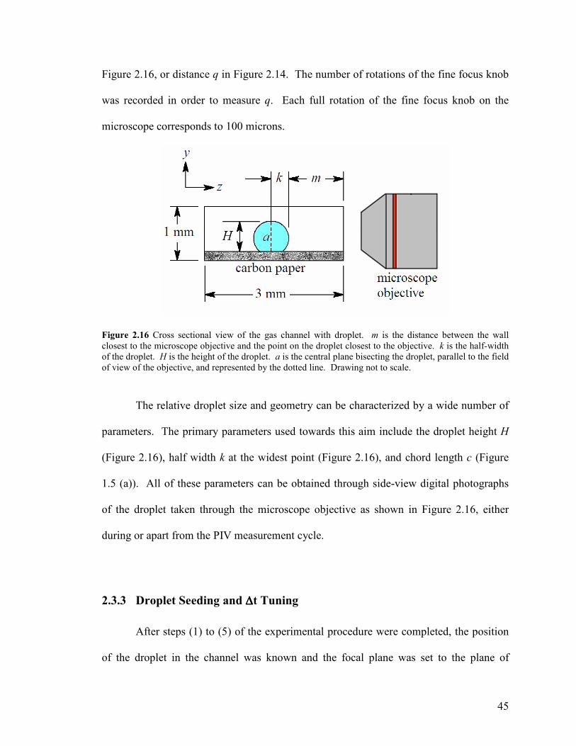
45

Figure 2.16, or distance q in Figure 2.14. The number of rotations of the fine focus knob

was recorded in order to measure q. Each full rotation of the fine focus knob on the

microscope corresponds to 100 microns.

Figure 2.16 Cross sectional view of the gas channel with droplet. m is the distance between the wall

closest to the microscope objective and the point on the droplet closest to the objective. k is the half-width

of the droplet. H is the height of the droplet. a is the central plane bisecting the droplet, parallel to the field

of view of the objective, and represented by the dotted line. Drawing not to scale.

The relative droplet size and geometry can be characterized by a wide number of

parameters. The primary parameters used towards this aim include the droplet height H

(Figure 2.16), half width k at the widest point (Figure 2.16), and chord length c (Figure

1.5 (a)). All of these parameters can be obtained through side-view digital photographs

of the droplet taken through the microscope objective as shown in Figure 2.16, either

during or apart from the PIV measurement cycle.

2.3.3 Droplet Seeding and ∆∆∆∆t Tuning

After steps (1) to (5) of the experimental procedure were completed, the position

of the droplet in the channel was known and the focal plane was set to the plane of

46

interest. If the plane of interest corresponded to central plane a in Figure 2.16, under the

fluorescent light the droplet would be visible in the test section through the objective as

shown in Figure 2.17 (a). For a 0.35 microlitre droplet, the mean height measured from

over 166 independent droplets is approximately 0.7 mm. This dimension is shown in

Figure 2.17 (a) for a scale reference.

Figure 2.17 (a) Side view of a droplet sitting on the carbon paper surface of the gas channel in the test

section. This is what the microscope objective in Figs. 6 and 7 would see. (b) Side-view of a seeded

droplet under quiescent conditions with camera exposure adjusted to brighten particles. (c) The same

droplet from (b) exposed to an air flow from right to left. The exposure has been set very long to

exaggerate the streak lines. The air velocity is not sufficient here to noticeably deform the droplet shape.

Image in (a) is not at the same scale as in (b) and (c).

The water used to generate the droplets was seeded with the fluorescent tracer

particles, before the PIV experiment begins. Seeding is more of an art than a science.

For any given fluid velocity, a range of seeding densities can be used, each accurately

capturing the flow dynamics. For micro-DPIV, to avoid excess out-of-plane noise, it is

desirable to use the lowest seeding density possible before the vector calculation

algorithm in the software starts to produce regions of bad vectors. After a trial and error

process, it was found that the ideal seeding density for the conditions used in this

experiment was 0.0002 % by volume. A 0.35 microlitre droplet seeded at this density

under bright green halogen lighting conditions is shown in Figure 2.17 (b). In this case,

47

ambient lighting has been eliminated so that only light fluoresced by the tracer particles is

captured. The camera exposure and resolution has been adjusted to accentuate the

particles. Notice in Figure 2.17 (b) that some particles appear smudged, blurred, or

streaked due to optical distortion, interference, or out-of-plane noise. Moreover, seeding

particles should be sized so that they correspond to 2 pixels in the raw digital

photographs, but it is clear from Figure 2.17 (b) that this criteria is not met very well.

This would typically be considered poor quality seeding by conventional cross-

correlation standards, which is why the sum-of-correlation algorithm outlined in Section

2.1 will be used for the vector calculation.

Once air flow is initiated in the channel, shear forces from the air induced a

secondary flow in the droplet, causing the particles to move with the flow as illustrated

by the streaklines in Figure 2.17 (c). Before acquiring a set of PIV image pairs of this

flow, the ∆t parameter used for the vector field calculation had to be set in the DaVis PIV

software. The choice of ∆t depended on the speed of the fluid inside the droplet. For a

32 x 32 pixel interrogation window, it is preferable to have the shortest particle

displacement be on the order of 5 pixels and the longest on the order of 15 pixels. The ∆t

must be adjusted such that this condition is met for a given air flow rate.

2.3.4 Experimental Operating Conditions and Controlled Parameters

The primary controlled variable in this experiment was the air flow rate. After

steps (1) through (7) of the experimental procedure had been completed, the air flow was

ramped up from zero to the desired rate over a period of 3 to 5 seconds by hand using the

flow control valve (step (8)). Theodorakakos et al. resolved from their experiments that

48

increasing the flow from quiescent conditions to the desired rate over a period of 30 ms

or higher resulted in no significant effects on the droplet dynamics due specifically to the

air flow increase. Their experiments were conducted using flow velocities within the

same range as those used for this work [8].

Once the desired flow rate was reached, the laser was activated and the PIV image

capture sequence was initiated in the LaVision DaVis software. The camera captures

image pairs at a rate of about 5 Hz. The user may set the number of image pairs

acquired. For this work, 30 image pairs from the steady-state flow inside the droplet

were acquired per capture sequence for processing. These 30 pairs were used to calculate

a single average vector field based on the sum-of-correlation method described in Section

2.1. 30 pairs were chosen since after 30 pairs a perceptible, significant decrease in

droplet volume due to evaporation was observable. Droplet evaporation in the channel

was studied in an independent experiment, described in Appendix B.

A preliminary droplet shedding study was performed with the apparatus prior to

this micro-PIV work. Observation of 100 independent droplets shedding on the carbon

paper surface of two separate flow channels resulted in an average critical air velocity

sufficient for shedding of about 8.5 m/s. The details of this study are presented in

Appendix B. The correlation table for the rotameter flowmeter used can be found in

Appendix C.

Table 2.1 Air flow rates used in this experiment and corresponding ∆t settings in the DaVis PIV software.

Flow

rate

number

Flowmeter

setting ±±±± Air volume

flow rate

(mL/min)

±±±± (mL

/min)

Mean channel

air velocity

Uair (m/s)

±±±± (m/s)

Mean air

Reynolds

number

Reair

±±±±

1 20 3 400 50 2.2 0.3 210 30

2 40 3 760 50 4.2 0.3 410 30

3 50 3 930 50 5.2 0.3 500 30

4 60 3 1090 50 6.0 0.3 580 30

49

For the primary experiment, four different flow rates translating to mean channel

velocities below 8.5 m/s were used to generate secondary flows inside the droplets. The

air used in this experiment was at room temperature, approximately 23°C. Velocity field

measurements from the vertical central plane of symmetry (Figure 2.13) were acquired at

each of these flow rates. These flow rates are listed in Table 2.1, and have been

translated into mean channel air velocities based on the channel area of 1 mm x 3 mm.

These channel air velocities have also been translated into a Reynolds number defined as

in Section 2.3.2, based on the channel hydraulic diameter of 1.5 mm and the dynamic

viscosity ν = 1.56x10-5

m2/s for air at 25°C. The rotameter flowmeter readings are

accurate to ± 2% of full scale. Full scale is 150 marks on the scale, or 2300 mL/min.

Thus, flowmeter readings are accurate to ± 3 marks on the scale, or approximately ± 50

mL/min. This uncertainty is translated into a channel velocity uncertainty and a

Reynolds number uncertainty in Table 2.1 using standard error propagation methods.

Table 2.2 provides the number of trials acquired (i.e. the number of independent

droplets analyzed) for each flow rate in Table 2.1. The corresponding ∆t setting used to

capture image pairs at each flow rate is also provided in Table 2.2. In some cases, this

parameter was adjusted slightly throughout the course of repeating the experimental trials

in order to more finely tune the pixel displacement of the particle images in each

interrogation zone. This fine tuning of ∆t is not expected to have a significant impact on

the accuracy of the measurements.

50

Table 2.2 Number of trials acquired and ∆t setting used for each flow rate number.

Flow rate

number

Flowmeter setting Number of trials

acquired ∆∆∆∆t setting (µµµµs)

1 20 36 425

2 40 35 350-375

3 50 35 310-325

4 60 60 275-300

51

2.4 DPIV Data Processing

2.4.1 LaVision DaVis PIV Vector Processing Procedure and Settings

The first step taken in the processing of the raw particle image pairs was the

construction of a mask to filter out all information outside of the droplet. Masks were

drawn using a series of linear splines drawn by hand in the DaVis mask definition

module. Since each droplet analyzed had a different shape, a different mask had to be

drawn for every one. Figure 2.18 shows an example of an un-masked and masked raw

droplet image.

Figure 2.18 The left image shows a raw particle image of a droplet in the channel. The right image shows

the result of a mask drawn around the droplet. The blacked out area is not included in the micro-DPIV

processing calculations.

After the mask was defined for a droplet, the set of 30 particle image pairs were

sent to the batch pocessing module in the DaVis software. This module executes a set

number of operations on the raw image pairs. There were two operations executed on the

droplet images acquired for this experiment: 1) PIV sum-of-correlation, and 2) vector

52

post-processing. Each of these operations has a number of options, settings, and

parameters in the software that must be selected or adjusted before the batch processing is

executed.

The following options were selected for the PIV sum-of-correlation operation:

1) Adaptive multipass: This is a technique pioneered by Westerweel et al. [23] and

Scarano & Reithmuller [24]. Its purpose is to reduce the effect of velocity bias on

the calculated vector fields. Velocity bias is a well understood source of error for

the cross-correlation method. Particles residing in a particular interrogation

window in the first image of a PIV image pair are more likely to exit the

interrogation window by the time the second image is acquired if they are moving

at higher relative speeds. Thus, there is a bias towards lower magnitude

displacement measurements for the regular two-frame cross-correlation method.

The adaptive multipass method corrects for this velocity bias by performing several

passes, or iterations, of the cross correlation algorithm, while shifting and resizing

the correlation window between passes in order to reduce the number of particles

that may exit a given interrogation window. By using an adaptive multipass

method, Scarano et al. were able to decrease the minimum measurable displacement

by one third while increasing the maximum measurable displacement by a factor of

four. For this experiment, two passes were made. The first pass is performed with

an interrogation window size of 64x64 pixels. A displacement vector called a

‘predictor’ is acquired from this 64x64 window via cross-correlation. Each 64x64

pixel window is then divided into four 32x32 pixel windows. The second pass is

53

performed by shifting each group of four 32x32 pixel windows by an amount

corresponding to the predictor calculated in the first pass, and then performing the

cross correlation in those shifted windows. The predictor is added to each of the

four vectors acquired from the second pass to arrive at one final vector for each

32x32 pixel window. Restrictions on the degree of variation between the predictor

and the vectors from the second pass were imposed in the software. A relative

restriction of reference ± window size/2 and an absolute restriction of reference ± 5

pixels were imposed.

2) Interrogation window overlap: Hart [25] described a technique, which is

commonly called the second-order method, for reducing the impact of false

correlation peaks in noisy data by overlapping two neighbouring interrogation

windows by 50%. The two overlapping regions are multiplied. This has the effect

of amplifying any correlation peaks that are common to both windows while

dampening any peaks that are not. The method reduces the likelihood of acquiring

a false vector, but delivers a single averaged displacement vector between the two

correlations. It has been shown to be most appropriate when processing noisy data,

such as that acquired in this experiment. In this work, the interrogation window

overlap was set to 50% in the DaVis software, resulting in a final resolution of

16x16 pixels, or approximately 16x16 microns.

54

3) Standard FFT cross-correlation: The standard Fast Fourier Transform was selected

for performing the cross-correlation calculation for each interrogation window pair.

This transform is defined as

,2

,2

),,(),(),(,

0,0

21

ndydx

ndyydxxIyxIyxC

nymx

yx

<<−++⋅= ∑<<

==

(6)

where I1 and I2 are the intensities of the first and second interrogation windows in

an image pair respectively, C is the correlation strength for all integer displacements

between the two images, and n is the dimension of the interrogation window [26].

The other cross-correlation function available in the software is a normalized

version of the FFT, which is described as being most useful when there are high

degrees of varying background intensity, a characteristic not present in this

experiment. The standard version in equation (6) correlates approximately 5 times

faster than the normalized version.

4) Multipass vector filtering: After each pass of the adaptive multipass process, a

median filter was applied to the resultant displacement vector calculations. First a

low-pass filter was imposed to remove displacements that were greater than 2 times

the root-mean-square (rms) value of all of their immediate neighbours. Then, a re-

insertion of displacements less than 3 times the rms value of their immediate

neighbours was performed. All vector groups composed of less than 5 vectors were

then removed entirely. All empty spaces were re-filled by interpolation. Finally, a

3x3 window smoothing function was applied to each vector. Smoothing is

automatically performed during adaptive multipass, and the minimum amount of

smoothing was selected for this experiment.

55

After the PIV sum-of-correlation operation was completed, and a complete vector

field was achieved, the vector postprocessing operation was initiated utilizing the

following options:

1) Filtering: Vectors in the final vector field that were greater than 3 times the rms

value of their neighbours were removed.

2) Interpolation: All empty spots in the vector field were filled by interpolation.

2.4.2 Optical Distortion Correction

Since the light from the fluorescent particles had to pass through the curved

interface between the water droplet and the air, some optical distortion was present in the

raw captured images due to the difference in index of refraction between the two media.

An optical distortion correction scheme was written in Matlab for this work, based on the

work of Kang et al. and Minor et al. [27, 28]. The details behind the derivation of the

algorithm and its implementation in Matlab are presented in Appendix D. The algorithm

is based on optical ray-tracing principles. It works by pulling information from each

pixel in the distorted droplet image inwards to another pixel closer to the center of the

droplet to compensate for the bending of light outwards by the curved droplet surface.

The algorithm was modified to correct the resultant vector fields calculated by the DaVis

software directly.

56

Chapter 3 Results and Discussion

3.1 Side-View Center-Plane Flow Patterns

Figures 3.1 through 3.4 present examples of raw particle images, uncorrected

vector field results formatted for both DaVis and Matlab, and final vector field results

corrected for optical distortion from Matlab. The corrected images also show the original

vector field outline, and the idealized droplet shape used to perform the optical distortion

correction, as outlined in Appendix D. One set of examples is provided for each of the

four flow rates in Table 2.1. Note that for each flow rate, the fluid is moving in a quasi-

elliptical, circulating pattern around a low velocity point near the centroid of the droplet

shape. This point will be termed the ‘center of rotation’ for the purposes of this work.

The velocity vectors tend to increase in magnitude outwards from this point, such that the

highest magnitude vectors exist somewhere near or along the outer edge of the vector

field.

The position scales on the (a) and (b) components of Figures 3.1 through 3.4 are

not calibrated to any specific zero point and are provided for a size comparison only. The

position scales on the (c) and (d) Matlab components are zeroed at the center of the

droplet chord, which is the two-dimensional projection of the three phase contact line.

In Figure 3.3, some spurious vectors can be seen at the upper-left corner of the

field. These bad vectors are due to deviation of the actual droplet profile away from the

idealized shape. Adaptive droplet shape approximations would thus be required to

correct the vector fields to a higher degree of accuracy.

57

(a)

(b)

58

(c)

(d)

Figure 3.1 (a) Example of raw particle image for mean air velocity of 2.2 m/s. (b) Vector field

corresponding to raw image. (c) Uncorrected vector field as imported into Matlab. Both axes are in meters.

(d) Vector field corrected for optical distortion, showing original vector field outline (thick red line), and

idealized droplet shape used for distortion correction (contour plot).

59

(a)

(b)

60

(c)

(d)





61

(a)

(b)

62

(c)

(d)





63

(a)

(b)

64

(c)

(d)





65

3.2 Side-View Center Plane Parametric Studies

3.2.1 Droplet Geometry

Due to the uncertainty of the micropipette, unavoidable droplet evaporation

during each trial setup, and the irregular nature of the carbon paper surface onto which

the droplets were placed, the droplet size and geometry was not constant between each

trial. This fact also becomes obvious when comparing the droplet in Figure 3.4 to the

droplet in Figure 3.1. The former droplet is shorter in height and has a longer contact line

than the latter. The droplet geometry and volume statistics extracted from the raw

particle images from all of the trials are presented in Table 3.1. The volume was

estimated from the height and chord length using the ideal droplet approximation

discussed in Appendix A.

Table 3.1 Average droplet dimensions and estimated volume.

Flow

Rate

Average

height (mm)

Std. dev.

(mm)

Average chord

length (mm)

Std. dev.

(mm)

Average

volume* (µµµµL) Std. dev.

(µµµµL) 1 0.72 0.04 0.71 0.09 0.37 0.04

2 0.69 0.05 0.69 0.09 0.33 0.06

3 0.69 0.05 0.63 0.10 0.31 0.05

4 0.72 0.05 0.69 0.10 0.34** 0.06** * See Appendix A for volume approximation method.

**These values were acquired from a sub-sample of 34 trials from the total sample population of 60 trials.

Notice in Table 3.1 that the average droplet height is fairly repeatable and close to

700 microns, but there is quite a wide deviation in the measured chord lengths. Chords as

wide as 970 microns and as narrow as 500 microns have been observed. There is a

degree of variation in the mean droplet volume between the trials, but it does tend to

hover around the 0.35 microlitre setting on the micropipette. This variation in droplet

geometry stresses the importance of approaching two-phase droplet and air flow studies

66

in small channels using a statistical averaging approach, since exact droplet geometries

are hardly ever repeatable.

3.2.2 Contact Angle Hysteresis

Notice in Figure 3.1 (d) that the actual droplet profile is fairly close to the

idealized shape used to perform the distortion correction, but as the air flow is increased,

the droplet begins to deform away from the idealized shape, as evidenced especially in

Figure 3.3 (d). Table 3.2 presents results from contact angle measurements performed on

a sub-sample of the droplets photographed for the primary micro-PIV measurements.

The contact angle measurement technique is outlined in Appendix E. The sub-sample

size is presented for each flow rate.

Table 3.2 Results from contact angle measurements performed on the droplet image sub-samples.

Flow

Rate

Sub-

sample

size (#)

Average

advancing

contact angle

(deg)

Std.

dev.

(deg)

Average

receding

contact angle

(deg)

Std.

dev.

(deg)

Average

contact angle

hysteresis

(deg)

Std.

dev.

(deg)

1 18 121 10 114 11 8 7

2 16 116 14 100 14 19 12

3 15 125 11 103 6 22 13

4 20 126 15 98 14 28 14

Again, the uneven nature of the carbon paper surface contributes to a wide

distribution of observed contact angles. However, it is clear that the average contact

angle hysteresis, or the difference between the advancing and receding contact angles,

increases with increasing air flow rate, indicating that the droplets in general experience a

higher degree of deformation when exposed to stronger forces from the air flow.

67

3.2.3 Peak Velocity

Intuitively, it makes sense that a higher air flow rate should induce a higher peak

velocity in the center plane of the droplet, as shear forces from the air phase pull the fluid

inside the droplet along at a faster rate. Figure 3.5 presents the maximum, minimum, and

average peak velocity, from each set of distortion-corrected vector fields acquired at the

four air flow rates. The data from Figure 3.5 is also presented in Table 3.3.

Vector Field Peak Velocity vs. Air Velocity

0.000

0.020

0.040

0.060

0.080

0.100

0.120

1.0 2.0 3.0 4.0 5.0 6.0 7.0

Air Velocity (m/s)

Peak Liquid

Velocity (m/s)

Max Peak Velocity

Min Peak Velocity

Average Peak Velocity

Figure 3.5 Maximum, minimum, and average peak velocity from each of the four sets of distortion-

corrected vector fields acquired. The error bars on the average peak velocity data points come from the

standard deviation of the peak velocity data at those air velocities.

Table 3.3 Raw data from Figure 3.5.

Flow

Rate

Air velocity

(m/s)

Maximum peak

liquid velocity

(m/s)

Minimum peak

liquid velocity

(m/s)

Average peak

liquid velocity

(m/s)

Std.

dev.

(m/s)

1 2.2 0.049 0.026 0.034 0.005

2 4.2 0.071 0.029 0.049 0.008

3 5.2 0.088 0.034 0.058 0.014

4 6.0 0.105 0.034 0.059 0.014

68

Note from Figure 3.5 that both the maximum observed peak liquid velocity, the

standard deviation about the average, and the range of peak velocities (difference

between max and min) increase continuously with increasing air flow. The wider

distribution in the observed peaks might be indicative of a flow regime change or an

increased degree of instability in the flow inside the droplet due to the increasing stress

applied to the droplet from the air flow. Moreover, note that degree of increase in the

average velocity tends to taper at the highest two air flow rates.

3.2.4 U-Component Vertical Velocity Profiles

The u-component velocity profile, parallel to the y-axis and passing through the

‘center of rotation’ of each droplet, as shown in the sketch of Figure 1.5 (c), was

extracted from each vector field result. A subset of these velocity profiles was created by

removing any profiles originating from vector fields with obvious bad regions and high

bad vector counts. The remaining subset of good u-component profiles was binned into

two groups, based on the physical height of the top of the corrected vector field from

which the profile was extracted. The first group, which will be called group ‘A’ came

from droplets with heights ranging between 570 and 610 microns. The second group,

called group ‘B’ came from vector fields with heights ranging between 530 and 570

microns. The velocity profiles from each of these groups were averaged for each of the

four flow rates used in the experiment, and are presented in Figure 3.6. The subset size

for each flow rate is provided in the legend of the graphs.

69

Average Vertical u-Velocity Profile at Center of Rotation

Group A (570 to 610 microns)

0

100

200

300

400

500

600

700

-0.04 -0.03 -0.02 -0.01 0 0.01 0.02 0.03 0.04

Liquid u-velocity (m/s)

y-position (microns)

2.2 m/s air flow - 13 Trials




(a)

Average Vertical u-Velocity Profile at Center of Rotation

Group B (530 to 570 microns)

0

100

200

300

400

500

600

-0.04 -0.03 -0.02 -0.01 0 0.01 0.02 0.03 0.04

Liquid u-velocity (m/s)

y-position (microns)





(b)

Figure 3.6 (a) Group A averaged u-component velocity profiles passing through the centre of rotation of

each droplet. Corrected vector fields in this group had heights ranging between 570 and 610 microns. (b)

Group B averaged u-component velocity profiles passing through the centre of rotation of each droplet.

Corrected vector fields in this group had heights ranging between 530 and 570 microns.

70

Notice first that the general shape of all of the plots very closely resembles the

hypothesized truncated “S”-shaped inside the droplet sketched in Figure 1.5 (c).

However, there seems to be some degree of “bend-back” in the velocity profile that

occurs systematically for each profile near the top of the vector field. This decrease in u-

component velocity is highly counterintuitive and might be due to a number of factors.

Firstly, the u-component profiles are extracted from velocity fields of varying

heights, as explained above. Thus, there may not be enough data points in the top region

of the profiles to accurately represent the true velocity. Second, the velocity

measurements from the top of the vector fields come from a highly distorted region of the

droplet very close to the gas-liquid interface, which then has an additional uncertainty

imposed on it due to the distortion correction algorithm, which assumes an ideal droplet

shape. There are too many factors at play preventing a scientific conclusion from the

bend-back trend in the velocity profile. As such, data in this region will not be

considered further in this study.

Another very important trend to observe is the fact that, for both Group A and B,

the slope of the velocity profile does not change as drastically between the last two air

flow rates (5.2 and 6.0 m/s) as it does between the first three. Intuitively, one would

expect the slope of the profile to continue to increase with increasing air flow rate, as the

shear forces from the air flow drive the liquid along at an increasing rate in the center

plane. This does not seem to be the case, however.

71

Liquid u-Velocity vs. Air Velocity

Group A (570 to 610 microns)

at specified y-position in droplet center plane

-0.06

-0.04

-0.02

0

0.02

0.04

0.06

0.0 1.0 2.0 3.0 4.0 5.0 6.0 7.0

Air Velocity (m/s)

Liquid u-Velocity (m/s)

y-position = 510 microns


(a)

Liquid u-Velocity vs. Air Velocity

Group B (530 to 570 microns)

at specified y-position in droplet center plane

-0.06

-0.04

-0.02

0

0.02

0.04

0.06

0.0 1.0 2.0 3.0 4.0 5.0 6.0 7.0

Air Velocity (m/s)

Liquid u-Velocity (m/s)



(b)

Figure 3.7 (a) Liquid u-Velocity vs. Air Velocity for group A at two specific y-positions from the carbon

paper surface, 138 microns and 512 microns. (b) Liquid u-Velocity vs. Air Velocity for group B at two

specific y-positions from the carbon paper surface, 140 microns and 510 microns. Liquid velocity error

bars come from the standard deviation of the subset of velocity profiles at each air flow rate, at the given y-

position.

72

The u-component velocity at heights of 140 and 510 microns from the carbon

paper surface were plotted against air velocity for the two groups of results. 140 microns

was chosen for the lower height because it corresponds roughly with the bulge in the

lower part of the “S” shape in the velocity profile, while 510 microns was chosen for the

upper height because it corresponds roughly to the highest common point between all

profiles before the “bend-back” phenomenon occurs. These plots are shown in Figure

3.7.

These plots clearly illustrate the decrease in the acceleration of the fluid as air

velocity is ramped up between 5.2 and 6.0 m/s. In some cases, the velocity at these

heights actually decreases with increasing air flow rate. The error bars in Figure 3.7 and

47 come from the standard deviation of the subset of trials used to produce each velocity

profile, at the particular y-position under study. It is especially interesting to note that

this taper in the fluid acceleration is also mirrored in the plot of average peak velocity in

Figure 3.5.

3.2.5 Distribution of Highest Magnitude Velocity Vectors

In order to better determine if there is, in fact, a general flow regime change

causing this taper in the acceleration of the fluid in the central plane with increasing air

flow rate, a study was performed on the physical distribution of the highest velocity

vectors in each vector field. A binary image was produced from each individual vector

field, at the same resolution as the vector field. A white ‘1’ was placed at each location

in the field where a velocity vector in the top 30% of the scale is discovered, while a

73

black ‘0’ is placed at all other locations. All of the binary images for each air flow rate

were superimposed to create four binary maps showing the physical distribution of the

top 30% of the vectors.

Figure 3.8 Physical distribution of the top 30% of the velocity vectors from all trials at each air flow rate.

For the highest flow rate, 6.0 m/s, a sub-sample of 35 trials was used to produce

the map; for all other flow rates, all available trials were used. The four maps are shown

74

in Figure 3.8. The average idealized droplet profile used to perform the distortion

correction for each air flow rate is included in the background of each velocity

distribution map for a reference.

It is clear from Figure 3.8 that the highest velocity regions from each vector field

are much more widely distributed at increasing air velocities. This may be indicative of a

flow regime change. In order to confirm that the results are repeatable, a similar map was

created from the remaining 25 trials available at the air flow rate of 6.0 m/s. The two

maps are compared in Figure 3.9. Although no formal pattern matching was performed

on the two images in Figure 3.9, its clear that the velocity vectors are distributed in

almost the same physical pattern at the air flow rate of 6.0 m/s.

Figure 3.9 Physical distribution of the top 30% of the velocity vectors from the last 25 trials and the first

35 trials acquired for the air flow rate of 6.0 m/s.

75

3.3 Discussion of Micro-DPIV Results

The micro-DPIV results have shown, in general, that the air flow induces a

rotational motion inside the droplet at the central plane of symmetry. A widening

physical distribution of the top 30% of the velocity vectors in the measured vector fields,

as well as a general taper of the liquid acceleration, has been observed while increasing

air flow rate. This is coupled with a general increase in standard deviation in the velocity

results at higher air flow rates. All of these factors could potentially point to a flow

regime change inside the droplet at increasing air flow rates, with changing contributions

to and from out-of-plane flow fields.

In the initial stages of the experiment, an increased degree of physical vibration

was observed at the air-liquid interface when it was exposed to higher air flow rates.

This induced physical instability may have caused an increased degree of uncertainty due

to measurements in undesired planes of flow offset from the central plane. Alternatively,

it is possible that the increased pressures inside the gas channel may have caused some

outwards deflection of the channel walls, marginally increasing cross sectional channel

area, but decreasing average channel velocity relative to a rigid wall channel. The author

of this work considers this to be highly unlikely, since no noticeable deflections were

ever observed from the raw PIV images.

Regardless, the increasing liquid velocity observed at increasing air flow rates,

and the increased degree of instability in the results, are caused by energy being added to

the droplet from the air flow. This energy can only be added by interaction between the

liquid and air phases at the interface. The induced liquid velocities measured in this

study are, in general, about 2 orders of magnitude lower than the channel-averaged air

76

phase velocity. It is impossible to comment on the impact of this secondary flow on the

forces experienced by the droplet without knowing the air phase velocity field, and

without performing an identical experiment using a solid droplet rather than a liquid. The

above factors stress the importance of continuing study on both the gas and liquid phases,

and the interactions at the interface, in order to better characterize the dynamics of such

droplet-in-air-flow systems.

Due to the methods used in this experiment, the velocity of the liquid in the

central plane of symmetry very near the interface between the droplet and the air was not

obtained. In future studies, this may be accomplished by performing single-point

velocity measurements of particles at the interface using a top-view rather than side-view

orientation. An example of a preliminary top-view measurement is demonstrated in

Appendix F.

77

Chapter 4 Conclusions and Recommendations

The three primary goals of the experiment will be addressed here, one at a time,

with a summary of how these goals were fulfilled.

1) Develop a method for applying 2-D micro-digital-particle-image-velocimetry (micro-

DPIV) techniques towards the qualitative and quantitative visualization of the

secondary flows induced inside the liquid phase for the case of air flow around a

droplet adhered to the porous bottom wall of a PEMFC gas channel model.

As outlined in this thesis, a method was developed for fabricating a model of an

optically transparent PEMFC gas channel, using relatively cheap materials and in-lab

fabrication techniques. This channel model was effectively designed for integration with

a micro-DPIV system that included an inverted microscope for flow visualization. A

method for performing a repeatable raw PIV image collection trial using this apparatus

was devised. The apparatus developed also proved to be useful for qualitative particle

streak imaging of the flows. The PIV sum-of-correlation algorithm was chosen, and

proved to produce, on the average, readable, repeatable, and physically intuitive vector

fields of the flow in the central plane of the droplets analyzed from the raw images. One

important contribution that arose from this work was the derivation of an optical

distortion algorithm with broader generality that the method available to date; this

algorithm accounts in particular for situations when the droplet is quasi-hemispherical as

is the case for hydrophobic surfaces. The algorithm was implemented in Matlab and

78

validates prior to its application to the processed vector fields. The combination of all of

the elements discussed above comprised a technique that proved to be adequate for

meeting the first goal of this work.

2) Acquire a relevant set of data from the experimental technique that could be

compared to results from a computational simulation of the same flow scenario.

As mentioned above, micro-DPIV was used to investigate the velocity field inside

the central plane of symmetry of a droplet adhering to a hydrophobic porous wall of a

rectangular gas channel, and exposed to an air flow. Various relationships between liquid

velocity, contact angle hysteresis, and the probability of a droplet shedding event with

respect to the air flow rate in the channel were derived from the measurements. Two-

phase CFD simulations of the same event can be compared to these results in order to

determine inconsistencies between the computational and experimental approaches.

Recent work by Zhu et al. highlights a method for applying the VOF (Volume of Fluid)

method in FLUENT towards a near identical droplet-in-channel flow scenario. Only a

few parameters in this study, such as the air velocity, droplet volume, channel dimensions

and surface properties, would need to be tweaked in order to make the results directly

comparable [29].

3) Investigate and/or suggest further avenues of study possible by using or modifying

the methods developed for the experiment, including an improved force balance

model.

79

As mentioned, it was not possible to make any velocity measurements very close

to the interface between the liquid and the air, and it is highly recommended that further

research be conducted in this avenue. Any discontinuity or ‘slip’ at the interface will

have a significant effect on the approach to modelling the drag forces on the droplet. In

order to improve the force balance model, it will be necessary to perform micro-DPIV

not only at more flow planes inside the droplet, but also ultimately in the air phase. This

work may yield additional terms or correction factors that may be used to modify the

original control volume force balance suggested by Kumbur et al. and Chen et al. to

account for the motion of the fluid inside the droplet.

80

References

[1] Eikerling, M., Kornyshev, A., and Kulikovsky, A., 2005, Can theory help us to

improve fuel cells?, The Fuel Cell Review, Dec. 2004 / Jan. 2005, pp. 15-23.

[2] Nguyen, T. and White, R., 1993, A water and heat management model for proton-

exchange-membrane fuel cells, Journal of the Electrochemical Society, vol.

140, pp. 2178-2186.

[3] Yang, X. G., Zhang, F. Y., Lubawy, A. L., and Wang, C. Y., 2004, Visualization of

liquid water transport in a PEFC, Electrochemical and Solid-State Letters, vol.

7, pp. A408-A411.

[4] Liu, X., Guo, H., and Ma, C., 2005, Water flooding and two phase flow in cathode

channels of proton exchange membrane fuel cells, Journal of Power Sources,

vol. 156, pp. 267-280.

[5] Tuber, K., Pocza, D., and Hebling, C., 2003, Visualization of water buildup in the

cathode of a transparent PEM fuel cell, Journal of Power Sources, vol. 124, pp.

403-414.

[6] Barbir, F., PEM Fuel Cells: Theory and Practice. San Diego: Elsevier, 2005.

[7] Kumbur, E. C., Sharp, K. V., and Mench, M. M., 2006, Liquid droplet behaviour

and instability in a polymer electrolyte fuel cell flow channel, Journal of Power

Sources, vol. 161, pp. 333-345.

[8] Theodorakakos, A., Ous, T., Gavaises, M., Nouri, J. M., Nikolopoulos, N.,

Yanagihara, H., 2006, Dynamics of water droplets detached from porous

surfaces of relevance to PEM fuel cells, Journal of Colloid and Interface

Science, vol. 300, pp. 673-687.

[9] Litster, S., Sinton, D., and Djilali, N., 2006, Ex situ visualization of liquid water

transport in PEM fuel cell gas diffusion layers, Journal of Power Sources, vol.

154, pp. 95-105.

[10] Bazylak, A., Sinton, D., and Djilali, N., Dynamics water transport and water

emergence in PEMFC gas diffusion layers, Journal of Power Sources, In Press

[11] Horton, T. J., Fritsch, T. R., and Kintner, R. C., 1965, Experimental determination

of circulation velocities inside drops, Canadian Journal of Chemical

Engineering vol. 43, pp. 143-146.

81

[12] Chen, K. S., Hickner, M. A., and Noble, D. R., 2005, Simplified models for

predicting the onset of liquid water droplet instability at the gas diffusion layer /

gas flow channel interface, International Journal of Energy Research, vol. 29,

pp. 1113-1132.

[13] Westerweel, J., 1997, Fundamentals of digital particle image velocimetry.

Measurement Science and Technology, vol. 8, pp. 1379-1392.

[14] Sinton, D., 2004, Microscale flow visualization, Microfluidics and Nanofluidics,

vol. 1, pp. 2-21.

[15] LaVision, Device-Manual for Davis 7.0: Micro PIV. Göttingen: GmbH, 2004.

[16] Spring, K. R., and Davidson, M. W., Nikon, Depth of field and depth of focus,

2000, http://www.microscopyu.com/articles/formulas/formulasfielddepth.html.

[17] Fuchs, N. A., The Mechanics of Aerosols. Oxford: Pergamon Press, Ltd., 1964.

[18] Hinds, W. C., Aerosol Technology: Properties, Behavior and Measurement of

Airborne Particles, Second Edition. New York: John Wiley & Sons, Inc., 1998.

[19] Collins, L. R., Keswani, A., 2004, Reynolds number scaling of particle clustering in

turbulent aerosols, New Journal of Physics, vol. 6, p. 119.

[20] McDonald, J. C., Duffy, D. C., Anderson, J. R., Chiu, D. T., Wu, H., Schueller, O.

J. A., Whitesides, G. M., 2000, Fabrication of microfluidic systems in

poly(dimethylsiloxane), Electrophoresis, vol . 21, pp. 27-40.

[21] Reznik, S. N., Yarin, A. L., 2001, Spreading of a viscous drop due to gravity and

capillarity on a horizontal or an inclined dry wall, Physics of Fluids, vol. 14,

pp. 118-132.

[22] Nguyen, N. T. and Wereley, S. T., Fundamentals and applications of microfluidics.

Boston: Artech House, 2002.

[23] Westerweel, J., Dabiri, D., and Gharib, M., 1997, The effect of a discrete window

offset on the accuracy of cross correlation analysis of digital PIV recordings,

Experiments in Fluids, vol. 23, pp. 20-28.

[24] Scarano, F. and Reithmuller, M. L., 1999, Iterative multigrid approach in PIV

image processing with discrete window offset, Experiments in Fluids, vol. 26,

pp. 513-523.

[25] Hart, D. P., 2000, PIV error correction, Experiments in Fluids, vol. 29, pp. 13-22.

82

[26] Martin, J., P. Oshkai and N. Djilali, 2005, Flow structures in a u-shaped fuel cell

flow channel: quantitative visualization using particle image velocimetry, ASME

J. Fuel Cell Science & Technology, vol. 2, pp. 70-80.

[27] Kang, K. H., Lee, S. J., Lee, C. M., and Kang, I. S., Quantitative visualization of

flow inside an evaporating droplet using the ray tracing method, Measurement

Science and Technology, vol. 15, pp. 1104-1112, 2004.

[28] Minor, G., Oshkai, P., and Djiali, N., 2007 Optical distortion correction for liquid

droplet visualisation using the ray tracing method: further considerations,

Measurement Science and Technology, (in print).

[29] Zhu, X., Sui, P. C., and Djilali, N., 2007, Numerical simulation of emergence of a

water droplet from a pore into a microchannel gas stream, Micro Nanofluidics

(in print).

[30] Stalder, A. F., Kulik, G., Sage, D., Barbieri, L., and Hoffmann, P., 2006, A Snake-

Based Approach to Accurate Determination of Both Contact Points and Contact

Angles, Colloids And Surfaces A: Physicochemical And Engineering Aspects,

vol. 286, pp. 92-103.

83

Appendix A Droplet Evaporation Study

Prior to the primary micro-DPIV experiment, a short preliminary study was

performed in order to approximate the rate of evaporation of a liquid water drop under

conditions similar to those from the primary experiment, described in Section 2.3. It was

necessary to know how quickly a water droplet would evaporate, since, in the ideal case,

a constant-volume droplet was desired for the micro-DPIV imaging. A significant loss in

droplet volume would change the geometry of the flow and may have resulted in a

fundamental flow regime change either in the liquid phase or the gas phase.

For this evaporation experiment, a time series of photographs of an evaporating

droplet were acquired, and droplet dimensions were extracted from the photographs.

From these dimensions, the droplet volume could be estimated, and plotted in time

according to the photographic series. Since a water droplet adhering to the GDL bottom

wall in the channel has a shape that deviates from that of a perfect sphere, it was first

necessary to derive an approximation of the droplet volume based on dimensions that

were extractable from the photographic time series.

Figure A.1 depicts the geometry of an idealized droplet adhered to a hydrophobic

surface. The Cartesian axes, and the spherical polar co-ordinates for a point P on the

droplet surface are both shown.

84

Figure A.1 The geometry of a droplet with a height H much greater than its contact line radius R, where H

= R + b.. A point P sitting on the surface of the droplet is defined in polar co-ordinates by radius r polar

angle θ, and azimuthal angle φ. The droplet profile in any r-θ plane (including the x-y plane) is defined by

the shape function ζ(θ).

Consider the parametric equation for the profile of the droplet in Figure A.1, in

spherical polar co-ordinates, as defined in [27]:

0)(),( =−= θζθ rrF (A1)

F(r, θ) is a function containing the radial polar co-ordinate r and a shape function ζ(θ). It

defines the surface of the droplet in any r-θ plane when set equal to 0.

The shape function ζ(θ) is represented by a sum of the cosine series:

.coscos)(1

θθθζ bRkbRN

k

k +≅+= ∑=

(A2)

Note that the same convention for radius r, polar angle θ, and azimuthal angle φ used in

[27] will be used here. R is the contact line radius, as shown in Figure A.1. According to

[27], most droplet surfaces can be well represented using ζ(θ) = R + bcosθ. b is a factor

in the shape function ζ(θ) that determines the degree of deviation in the droplet away

from that of a hemisphere. Along the y-axis, the droplet height H is equal to R + b

according to equation (A1). This is illustrated graphically in Figure A.1. Dimensions H

85

and R can be acquired directly from side-view digital photographs of a droplet, as seen by

the microscope objective in Figure 2.16. These digital photographs are similar to those

shown in Figure 2.17 (a), and pixel-to-pixel distances can be extracted from them using

the DaVis PIV software.

To derive an equation for the volume of the droplet in Figure A.1, we start by

defining an infinitesimal volume element dV based on the shape function ζ(θ) in the r-

θ plane:

( )( ) .sincossin

sin)(

2

2

2

dybR

dy

dyrdV

θθθπ

θθζπ

π

+=

=

=

(A3)

y can be defined using the shape function as

θθζ cos)(=y (A4)

dy can be acquired implicitly by performing the following derivative

( )

.)cossin2sin(

cossin2sin

coscos 2

θθθθθθθ

θθθθ

dbRdy

bR

bRd

d

d

dy

−−=

−−=

+=

(A5)

Thus,

( ) ,)cossin2sin(sincossin2 θθθθθθθπ dbRbRdV −−+= (A6)

and

( ) .)cossin2sin(sincossin2

0

2

∫ −−+=

π

θθθθθθθπ dbRbRV (A7)

86

The absolute brackets were added to equation (A7) since it is nonsensical to have a

negative value for a volume. Finally, we arrive at

.6

1

3

2

3

2 3223 bRbbRRV ππππ +++= (A8)

Equation (A8) can be validated intuitively by considering the case of a perfectly

hemispherical droplet, defined as such when b = 0. In this case, (A8) would reduce to

,3

4

2

1

3

2 33

== RRV ππ (A9)

which, is exactly half of the volume of a perfect sphere of radius equal to half the chord

length R. For further validation, consider dimension measurements taken from an actual

droplet photograph similar to that in Figure 2.17 (a). The volume of the droplet will be

approximated using equation (A8), and then, for comparison, approximated again using

the equation of a perfect sphere. The half-width of the droplet, defined as k in Figure

2.16, will be used to approximate the radius of the perfect sphere approximation for the

droplet. This comparison is made in Table A.1.

Table A.1 Measurements of R, b, and k from an actual droplet photograph, and the droplet volume

approximation results from equation (A8) compared to the perfect sphere assumption.

Parameter Value

R (Figure A1) 311 microns (measured)

B (Figure A1) 527 microns (measured)

k (Figure 2.16) 467 microns (measured)

3223

6

1

3

2

3

2bRbbRRV ππππ +++≅ (equation (A8)) 0.481 µL

≅ 3

3

4kV π (2 x equation (A9)) 0.426 µL

It’s clear from Table A.1 that the spherical approximation result differs from the

equation (A8) result by over 11%, which is quite significant. Thus, it is prudent to

87

employ the more detailed approximation to the droplet volume in (A8) instead of the

simpler spherical approximation.

Table A.2 Droplet position q and approximated starting volume.

Trial Measured Droplet Position q

(Figure 2.14) (mm)

Approximated Droplet

Starting Volume (µL)

1 1.45 ± 0.03 0.35

2 1.85 ± 0.03 0.45

3 1.50 ± 0.03 0.35

4 1.90 ± 0.03 0.40

5 1.85 ± 0.03 0.52

6 1.70 ± 0.03 0.58

7 1.10 ± 0.03 0.43

For the evaporation experiment, seven different droplets were placed by

micropipette into the side-view channel outlined in Section 2.2.3, one per evaporation

trial. The droplets were all placed beyond 3 cm from the air inlet (see dimension q in

Figure 2.14), where the air flow would be fully developed as demonstrated in Section

2.3.2. Table A.2 provides the droplet position q (Figure 2.14) and starting volume

approximated with equation (A8). The starting volume was difficult to control due to the

nature of the micropipetting process. For each trial, an air flow of about 2.5 m/s (channel

average) was initiated over the droplets in the channel. The droplets were photographed

in a time series using the CCD camera and microscope optics shown in Figure 2.1. The

first six droplets were photographed under light from the mercury arc lamp shown in

Figure 2.1. The first three of these were evaporated with dry air from the wall regulator.

The second three were evaporated with air that had passed through the bubbler humidifier

shown in Figure 2.1. The seventh droplet was evaporated with humidified air, and under

ambient room lighting conditions, with the mercury arc lamp turned off. The normalized

time series plots of the height and volume loss of the droplets are shown in Figures A.2

and A.3.

88

It’s clear from these plots that droplet lifetime in the channel is greatly enhanced

by adding the bubbler humidifier. Note that the evaporation rate demonstrated by Trial 4,

the first trial with the humidifier turned on, differs from Trials 5 and 6 in both figures.

This could be due to a discrepancy in the set flow rate. Regardless, it’s clear that the total

lifetime of the droplet in the channel is enhanced by a factor of about seven when the

humidifier is added.

Droplet Height Lost vs. Time

0%

20%

40%

60%

80%

100%

120%

0:00:00 0:02:53 0:05:46 0:08:38 0:11:31 0:14:24 0:17:17 0:20:10

Elapsed Time (h:m:s)

Height Lost (%)

Trial 1 - No HumidifierTrial 2 - No HumidifierTrial 3 - No HumidifierTrial 4 - HumidifierTrial 5 - HumidifierTrial 6 - HumidifierTrial 7 - Humidifier - No Arc Lamp

Figure A.2 Droplet height lost vs. time for the seven droplets used for this evaporation experiment.

89

Droplet Volume Lost vs. Time

0%

20%

40%

60%

80%

100%

120%

0:00:00 0:02:53 0:05:46 0:08:38 0:11:31 0:14:24 0:17:17 0:20:10

Elapsed Time (h:m:s)

Volume Lost (%)

Trial 1 - No HumidifierTrial 2 - No HumidifierTrial 3 - No HumidifierTrail 4 - HumidifierTrial 5 - HumidifierTrial 6 - HumidifierTrial 7 - Humidifier - No Arc Lamp

Figure A.3 Droplet volume lost vs. time for the seven droplets used for this evaporation experiment.

The mercury arc lamp, although useful for providing bright light for visualization,

does add a significant amount of heat to the test section. By turning off this lamp, and

using the lower intensity, cooler ambient fluorescent light of the room, the droplet

lifetime is again extended by a factor of about three during Trial 7. Since all ambient

lights in the room are turned off during the micro-DPIV experiment, it is fair to use this

trial to approximate the loss in droplet volume during a 30-image micro-DPIV capture

sequence, which runs for approximately 7 seconds.

According to the data from Trial 7, there is approximately a 2% height loss and a

4% volume loss during the first 17 seconds of exposure to the 2.5 m/s air flow. This rate

of volume loss would likely be increased at higher air flow rates. However, during the

actual PIV experiment, the acquisition sequence is only 7 seconds, and from the raw

90

images, a significant height loss greater than 4% was never observed at any air flow rate.

Moreover, the velocity field acquired from one such droplet is averaged over the 30

image pairs from the capture sequence using the sum-of-correlation algorithm outlined in

Section 2.1. Thus, it was deemed that droplet evaporation was not considered to be a

significant issue for the capture sequence lengths used in the primary experiment.

91

Appendix B Critical Shedding Air Flow Rate Study

Prior to the micro-DPIV experiment outlined in Section 2.3, a preliminary test

was performed in order to approximate the critical air flow rate at which a droplet

adhered to the GDL sidewall of the 1 mm x 3 mm gas channel would shed from the

surface of the GDL and advance in the direction of the air flow. Two different chips

were used to perform this test: (a) the primary chip outlined in Section 2.2.3 that permits

a side view of the droplet, and (b) a second chip of a different design, permitting a top

view of the droplet, as shown in the right-side image of Figure 2.12. These two chips

will herby be referred to as the ‘side-view’ and ‘top-view’ chips, respectively.

The procedure followed for one trial of this preliminary test is as follows: (1) A

single 0.35 microlitre droplets is pipetted into the gas channel of the chosen chip, (2) the

diameter and position of the droplet in the channel (Figure 2.14) are measured and

recorded, (3) the chip is coupled to the air flow tube and placed in the stage of the

inverted microscope, (4) the droplet in the channel is viewed in real time on the computed

screen (either from the side or the top depending on the chip used) via the CCD camera

and microscope optics, (5) the air flow is ramped up slowly from zero by hand using the

flow control valve of the rotameter, (6) when the droplet shedding event is observed on

the computer screen, the critical air flow rate on the rotameter is recorded, (7) the channel

is opened and blown clean with compressed air to prepare it for the next trial.

For the side-view chip, the droplet position in the channel, denoted by variables p

and q in Figure 2.14, were measured as described in Section 2.3.2. However, for the top-

view chip, the dimension q in Figure 2.14 was measured using scaled digital photographs

92

of the droplet in the channel. The z co-ordinate at the common channel sidewall (i.e.

closest to the objective in Figure 2.14) was recorded, and then the point of maximum

projected droplet width along the z-axis was recorded. The difference between these two

z co-ordinates was taken as the dimension q.

Critical Shed Flow Rate 1x3 Channel w/ GDL

100 Measurements (50 side view, 50 top view)

0%

5%

10%

15%

20%

25%

30%

35%

5.2 - 6.0

6.0 - 6.9

6.9 - 7.7

7.7 - 8.5

8.5 - 9.3

9.3 - 10.0

10.0 - 10.7

10.7 - 11.4

11.4 - 12.1

12.1 - 12.9

Air Velocity Range (m/s)

Count Percentage

Top View

Side View

Figure B.1 Chritical shedding air flow rate statistics for a 1 mm x 3 mm air flow channel with a GDL

sidewall. Droplet volume is 0.35 mm. Count percentage refers a percentage of the 50 trials acquired for

each chip. One count constitutes one observed shedding event.

Table B.1 Droplet position and size statistics.

Chip Number

of trials

Mean

droplet

diameter*

(mm)

Std.

dev.

(mm)

Mean

droplet

position

p** (cm)

Std.

dev.

(cm)

Mean

droplet

position

q** (mm)

Std.

dev.

(mm)

Mean critical

shed velocity

range (m/s)

(Figure B.2)

Top

view

50 0.73

± 0.005

0.07 4.1

± 0.1

0.3 1.58

± 0.03

0.08 9.3-10.0 m/s

Side

view

50 0.77

± 0.005

0.03 4.0

± 0.1

0.3 1.46

± 0.03

0.13 8.5-9.3 m/s

* Equivalent to 2b from Figure 2.16 (for an ideal, symmetric droplet), measured at the widest point of the

droplet.

** See Figure 2.14.

93

50 trials were performed for the side view chip and 50 were performed for the top

view chip. The critical air flow rates observed over the 100 trials were translated into

mean channel air velocities and statistically binned into velocity ranges that correspond to

the major divisions on the rotameter. The results of the shedding study are presented in

Figure B.1 and Table B.1. The uncertainty in measurement for mean droplet diameter

comes from an assumption that the measurement can be made accurately on screen

within 5 pixels, which equates approximately to 5 microns based on the scaling of the

images. The droplet position p measurement uncertainty is based on the 1 mm division

on the ruler used. The droplet position q uncertainty comes from the 30 micron depth of

field of the microscope objective.

Figure B.2 clearly shows a statistical distribution in the critical shedding velocity

range observed for each chip. If Normal distributions are assumed, it appears that the

peaks of these distributions are slightly offset. This could be due to a number of factors,

including some marginal differences in gravitational forces due to the change in droplet

orientation between the two chips, slight differences in channel cross section due to

manufacturing tolerances, local variations in GDL structure that change the forces

pinning the droplet to the GDL, and the fact that the number of trials acquired may not be

statistically significant. The 120-micron discrepancy between the mean q positions of the

chips demonstrated in Table B.1 could be attributed to the fact that the droplets were

placed in the channel and positioned by hand, or the fact that the technique for measuring

this dimension differed between the two chips.

94

Since the side view chip presents a lower mean critical shedding velocity range,

8.5-9.3 m/s, the lower limit of this range, 8.5 m/s was used to approximate the mean

critical shedding velocity for the purposes of the primary micro-DPIV experiment.

95

Appendix C Flowmeter Correlation Table

The rotameter flowmeter used for this experiment is the Omega FL-3804G. Table

C.1 presents the correlation table for this flowmeter, for dry air at 21°C and 101 kPa.

Table C.1 Correlation table for Omega FL-3804G for dry air at 23°C.

Flowmeter Scale Flow Rate (mL/min)

10 185

20 395

30 590

40 763

50 928

60 1085

70 1240

80 1392

90 1535

100 1674

110 1807

120 1932

130 2050

140 2170

150 2313

96

Appendix D Optical Distortion Correction Algorithm

In order to correct the optical distortion of particle light passing through the

curved interface between a water droplet surface and the surrounding air, it was first

necessary to perform some ray tracing to determine the angles of incidence and refraction

to be expected at the droplet surface. This ray tracing method will be outlined first in this

section, and then the image correction algorithm will be reviewed.

The first step in the ray tracing method is to determine the normal vector to the

surface of the droplet everywhere on the surface. A normal vector to the surface of the

idealized droplet in Figure A.1 may be derived from equations (A1) and (A2) in two

dimensions only, since (A1) and (A2) have no dependence on φ. We can derive an

expression for the normal vector N which will lie in the r-θ plane at any given azimuthal

angle φ as

F

F

∇∇

=N (A10)

where

θθθ

θeeee

r

bF

rr

FF rr

sin1+=

∂∂

+∂∂

=∇ , (A11)

and

r

brF

θ222 sin+=∇ . (A12)

Thus

θθ

θ

θeeN

222222 sin

sin

sin br

b

br

rr

++

+= . (A13)

97

Figure D.1 Radial and polar components of the normal vector shown in the plane φ = π/2, with respect to

the x- and y- axes indicated by the unit vectors i and j respectively.

The next step is to translate the normal vector in (A13) into Cartesian co-

ordinates, keeping in mind that our choices for φ will affect the respective magnitudes of

the individual components of the vector. If we choose our reference plane at φ = π/2 (or

z = 0), we can write the r- and θ -components of N in terms of Cartesian coordinates by

projecting them onto the x- and y- axes:

222

πφπφπφ ===+= θr NNN (A14)

j

iN

θθ

θθ

πφ

cossin

sinsin

222

2222

br

r

br

rr

++

+=

=

(A15)

.sinsin

sin

cossin

sin

222

2222

j

iN

θθ

θ

θθ

θπφθ

br

b

br

b

+−

+=

=

(A16)

Thus, using (A15) and (A16) to express (A14) in Cartesian coordinates we get

98

.sin

sincossin

sin

cos

222

2

2222

jiNθ

θθθ

θ

θπφ

br

br

br

br

+

−+

+

+=

= (A17)

The next step is to determine an expression for N at any angle 0 ≤ φ ≤ π/2. This will be

done by assuming that the i-component of (A17) retains the same magnitude but now

points in the direction of i*, which is a unit vector in the x-z plane pointing at an angle φ

from the z-axis. The j-component of (A17) doesn’t change with φ. Thus,

.sin

sincossin

sin

cos

222

2

22220

j*iNθ

θθθ

θ

θπφ

br

br

br

br

+

−+

+

+=

≤≤ (A18)

The i*-component of (A18) can then be broken up into i- and k-components to obtain

.cossinsin

cos

sin

sincos

sinsinsin

cos

222

222

2

22220

k

j

iNN

φθθ

θθ

θθ

φθθ

θπφ

br

br

br

br

br

br

+

++

+

−+

+

+==

≤≤

(A19)

Now that we have arrived at an equation for the normal vector to the surface of

the droplet, N, we can move on to derive the relationship between incident and refracted

rays of light at the surface of the droplet.

99

Figure D.2 Incident and refracted light beams A and B respectively, at the surface of the droplet. Vector

B is equal to the sum of vectors A and C. Vectors A, B, C and surface normal N all lie in plane S.

Figure D.2 shows the geometric relationship between the direction of an incident

light beam from the image plane, defined by the vector A, and the direction of the

refracted light beam inside the droplet which moves towards the corresponding point in

the object plane, defined by the vector B. To obtain the angle of incidence ψa of light

travelling from the image plane in the negative z-direction to the droplet surface, we

simply take the dot-product of the normal vector N in (A19) with A = –k

a222coscossin

sin

cosψφθ

θ

θ=

+

+−=⋅

br

brNA . (A20)

Thus,

.cossinsin

coscos

222

1

a

+

+= − φθ

θ

θψ

br

br (A21)

The angle of refraction ψd can then be obtained using Snell’s law [27], such that

.cos1cos 21

d

−= −

a

d

a

n

nψψ (A22)

100

The incident light beam on the droplet points in the direction of vector A. We

will now determine the components of the vector B which points in the direction of the

refracted light beam in the droplet after it has crossed the air-liquid interface. In order to

do this, we define a vector C perpendicular to A in the plane S of figure 3, such that B =

A + C. Next, we will determine a unit vector ec that points in the direction of C, such

that

.AAN

AANA

eA

CAB

da

da

××××

−+=

−+=

+=

)(

)()tan(

)tan(

ψψ

ψψ c (A23)

Allowing Ni, Nj and Nk to represent the scalar values of the i-, j-, and k-components of

(A19) respectfully, we have

.NN

N

NN

N

)(

)(

2

j

2

i

j

2

j

2

i

i ji

AAN

AANe

+

−+

+

−=

××××

=c

(A24)

Thus,

.NN

)Ntan(

NN

)Ntan(

2

j

2

i

jda

2

j

2

i

ida kj iB ++

−−+

+

−−=

ψψψψ (A25)

The common factor between the i and j terms of equation (A25), after substitution of Ni,

Nj and Nk and some simplification, will be defined as

.)sincos(sinsin)cos(

1

222222M

θθφθθ brbrf

−++= (A26)

Thus we have

101

.)sincos)(tan(

sinsin)cos)(tan(

2

daM

daM

kj

iB

+−−−

+−−=

θθψψ

φθθψψ

brf

brf (A27)

Knowing the relationship between the direction of incident light, -k, and refracted

light, B (equation (A26)) for all r, θ, and φ values, an algorithm can then be constructed

to correct distorted images.

Figure D.3 Tracing a ray of light, depicted with red lines, as it passes between a point Po in the object

plane and a point Pi in the image plane.

Consider fluorescent particles inside the droplet existing in the plane of focus, or

the object plane, which in the case of this experiment would be the central cross-sectional

plane of symmetry, or the vertical green plane in Figure D.3. This plane will be used as

the zero reference point along the z-axis. A particle existing at point Po = (xo, yo, 0) in the

object plane would emit light that would refract through the droplet-air interface, causing

the particle to appear to be at the point Pi = (xi, yi, zi) in the image plane of the camera.

102

The next step is to trace the path of light from this particle backwards from the

image plane to the object plane. We know that the light moves straight backwards from

Pi in the negative z-direction towards the interface, and intersects the interface at a point

Ps = (xi, yi, zs(xi, yi)) on the surface of the droplet, where zs(x, y) is a function defining the

surface of the droplet in Cartesian co-ordinates. The light then bends in the direction of,

B = (Bx, By, Bz), calculated using equation (A27) at the point Ps = (xi, yi, zs(xi, yi)) (after

converting this point to spherical polar co-ordinates). The distance travelled by the ray

inside the droplet as it moves towards the object plane would have three Cartesian

components, one of which would be zs(xi, yi) in the negative z-direction, since it must

travel from the point Ps = (xi, yi, zs(xi, yi)) back to the point Po = (xo, yo, 0). The remaining

two components can be found by applying the ratios of the vector components of B, such

that the x-component is ∆x = (Bx / Bz) zs(xi, yi) and the y-component is ∆y = (By / Bz) zs(xi,

yi). Notice in equation (A27) that the z-component of B, Bz, is actually 1, thus

),(),( iisiix yxzyxBx ⋅=Λ (A28)

),(),( iisiiy yxzyxBy ⋅=Λ (A29)

Thus, the algorithm to translate a point in the image plane to a point in the object

plane becomes quite simple:

),(),( iisiixi

io

yxzyxBx

xxx

⋅+=

Λ+= (A30)

),(),( iisiiyi

io

yxzyxBy

yyy

⋅+=

Λ+= (A31)

Moreover, by differentiating equations (A30) and (A31) with respect to time, we can

perform velocity mapping rather than image mapping:

103

i

iisiixi

i

iisiixii

i

o

o

)),(),(()),(),((

d

)d(

d

d

y

yxzyxBv

x

yxzyxBuu

t

xu

t

xu

∂

⋅∂+

∂

⋅∂+=

Λ+==

(A32)

i

iisiiy

i

i

iisiiy

ii

i

o

o

)),(),(()),(),((

d

)d(

d

d

y

yxzyxBv

x

yxzyxBuv

t

xv

t

xv

∂

⋅∂+

∂

⋅∂+=

Λ+==

(A33)

where uo and vo are the x- and y- velocities of the fluid in the plane, respectfully.

In order to perform the velocity mapping technique characterized by equations

(A32) and (A33) on a velocity field acquired by conducting micro-DPIV on a liquid

droplet as outlined in this work, it was necessary to know the surface function zs(x, y) of

the particular droplet under study. Based on the techniques developed for this work, it is

practically impossible to measure, with any degree of accuracy, the exact shape of the

interface of a liquid droplet sitting inside the gas channel model in three dimensions. In

order to simplify the process, the surface function zs(x, y) for each droplet was

approximated using the ideal droplet model characterized by equations (A1) and (A2) and

Figure A.1.

The distortion correction process used for the primary micro-DPIV experiment

begins with the vector field data exported from the DaVis software, after the image

capture sequence, sum-of-correlation vector field processing, and vector post processing

have been performed. This vector field data consists of u- and v-component velocity

information for each interrogation window inside the frame of acquisition. Interrogation

windows that are masked out during vector field processing contain zeroes for both of the

vector components. This vector field data is imported into Matlab.

104

Next, the outer profile of the non-masked region, which contains the vector field,

is found, and a boundary line is drawn around this region. This boundary line is used to

approximate the outer profile of the droplet in the channel, and thus provides the height H

and chord radius R necessary to create an idealized 3-D droplet model, as shown in

Figure A.1, for the droplet under study. An example of an un-corrected micro-DPIV

vector field imported into Matlab, with the boundary curve drawn around it, is shown in

Figure D.4. Notice in this Figure that the x and y co-ordinate system used to perform the

distortion correction is centered about the middle of the droplet chord, in order to

felicitate the modelling of the 3-D droplet shape with the ideal model of Figure A.1.

Figure D.4 Uncorrected micro-DPIV vector field from the center plane of a droplet in an air flow. Notice

that the x and y co-ordinate system has been centered at the middle of the droplet chord in order to felicitate

modelling of the droplet shape using the ideal model from Figure A.1.

105

The height H and chord radius R are then measured from the boundary line. At

higher air flow rates, the droplet deformation may be quite significant, and the x-

component symmetry of the droplet will be destroyed. The height of the droplet in this

case is approximated by the highest point in y of the drawn boundary, and the chord. The

chord radius R can be measured as normal, regardless of the degree of droplet distortion.

Equations (A1) and (A2) are then used to define the surface function zs(x, y) of the

droplet.

Next, the values for Bx and By are calculated at all points inside the bounded

region illustrated in Figure D.4, and the results are stored in separate matrices. A

corrected vector field is then generated by applying equations (A32) and (A33) to each

cell in the vector field matrix, within the bounded region. In the Matlab code

implementation of the correction algorithm, the partial derivatives in (A32) and (A33) are

approximated using a central difference. For example:

),(2

),(),(),(),(

)),(),((

2iisiixiis

i

iisiix

hOh

yhxzyhxByhxzyhxB

x

yxzyxB

iix +−⋅−−+⋅+

=

∂

⋅∂

(A34)

where h is the grid spacing, or the dimension of the square interrogation zones. The

corrected vector field corresponding to Figure D.4 is shown in Figure D.5.

The thick red curve in Figure D.5 shows the original droplet boundary drawn by

the Matlab program around the un-masked portion of the un-corrected vector field. The

contour plot represents the idealized 3-D droplet surface defining zs(x, y) used to perform

the correction. The corrected vector field has been truncated so that it only extends

outwards from the origin to 80% of the radius r of the shape, defined as in Figure A.1.

This truncation is performed because previous work by Kang et al. showed that the

106

correction scheme is only valid within about 80% of the droplet radius due to the high

degree of optical distortion and information loss very close to the edge of the

droplet.

Figure D.5 The corrected micro-DPIV vector field of Figure A8. The thick red curve shows the original

droplet boundary drawn by the Matlab program around the un-masked portion of the un-corrected vector

field. The contour plot represents the idealized 3-D droplet surface defining zs(x, y) used to perform the

correction. The corrected vector field has been truncated so that it only extends outwards from the origin to

80% of the radius r of the shape, where the radius of the shape is defined as in Figure A.1.

Another similar Matlab code was written to verify the vector correction code.

This verification code distorts a regular grid by applying the reverse of the image

mapping algorithm, characterized by equations (A30) and (A31). This distorted grid is

then corrected by applying the regular algorithm again. The results of this test are shown

107

in Figure D.6. Indeed, it is clear from the results that the information loss is too great

near the edges of the droplet, and thatonly about 80% of the distorted grid can be

reproduced.

Figure D.6 (a) Computer simulation of a regular grid bisecting an idealized water droplet. The grid lines

are distorted due to the refraction of the light passing through the interface of the droplet and the air. (b)

The same image after processing by a distortion correction algorithm. Notice that the original grid can only

be restored within about eighty percent of the radius of the droplet, due to the loss of information around

the far edge of the droplet from the distortion in (a).

The Matlab code for the correction program with comments is presented below:

BEGINNING OF MATLAB CODE %% Vector Field Processing for Center Plane Droplet Field %% %% Grant Minor 0528890 %% clc; clear; %% Code for determining droplet shape function %% % import vector field data in xls file % rawdata = xlsread('C:\Documents and Settings\minorgf\My Documents\Thesis Project\Vector Processing\April 5 Vector Results\053557.xls'); x = rawdata(:,1); y = rawdata(:,2); ui = rawdata(:,3); vi = rawdata(:,4); % create a new array for vector field domain with outline of droplet % % find x-width of domain in grid-points % i = 1; flag1 = 0;

108

while flag1 == 0 i = i + 1; if x(i) == x(1) flag1 = 1; end; end; xwidth = i - 1; % find y-width of domain in grid-points % ywidth = length(y)/xwidth; % make array uim, vim, and V of velocity magnitudes % for j = 1:ywidth for i = 1:xwidth uim(j,i) = ui(i + (j-1)*xwidth); vim(j,i) = vi(i + (j-1)*xwidth); V(j,i) = sqrt(uim(j,i)^2 + vim(j,i)^2); end; end; % find bottom of droplet and truncate matrix % heightcount = 0; for j = 0:(ywidth-1); if V(ywidth-j,xwidth/2) > 0; break; else heightcount = heightcount + 1; end; end; V = V(1:(ywidth-heightcount),:); ywidth = ywidth - heightcount; % find center of droplet chord % flag1 = 0; for i = 1:xwidth if V(ywidth, i) > 0 if flag1 == 0; flag1 = 1; chordfront = i; end; else if flag1 == 1; chordback = i-1; break; end; end; end; center = round((chordback - chordfront)/2); % create matrix of ones and zeroes defining droplet boundary with a 1 and % everywhere else with a zero outline = zeros(ywidth,xwidth); for j = 1:ywidth flag1 = 0; for i = 1:xwidth if V(j, i) > 0 outline(j,i) = 1; break; end; end; end; for i = 1:xwidth flag1 = 0; for j = 1:ywidth

109

if V(j, i) > 0 outline(j,i) = 1; break; end; end; end; for j = 1:ywidth flag1 = 0; for i = 1:xwidth if V(j, xwidth+1-i) > 0 outline(j,xwidth+1-i) = 1; break; end; end; end; for i = 1:xwidth flag1 = 0; for j = 1:ywidth if V(ywidth-j+1, i) > 0 if j == 1 break; else outline(ywidth-j+1, i) = 1; break; end; end; end; end; % find droplet height at center % height = 1; flag1 = 0; while flag1 == 0 if outline(height,round(chordfront+center)) == 1 flag1 = 1; else height = height + 1; end; end; dropheight = ywidth - (height - 1); R = round(abs(chordback - chordfront)/2); b = dropheight - R; % define ideal droplet shape function theta = 0:(2*pi/360):(pi/2); phi = R + b*cos(theta); %% End of Code for Determining Droplet Shape Function %% %% calculate all distances, radii, angles and trigonometric functions required for %% image correction algorithm % index of refraction of water = 1.33, for air = 1 % ls = 1.97e-5; % length scale % make a smaller matrix that includes only the droplet shape % % find leftmost and rightmost point on droplet % bottommark = ywidth; both_outlines = outline_sf + outline; topmark = bottommark;

110

for i = 1:xwidth for j = 1:ywidth if both_outlines(j,i) > 0 if j < topmark topmark = j; end; break; end; end; end; leftpoint = xwidth; for j = topmark:bottommark for i = 1:xwidth if both_outlines(j,i) > 0 if i < leftpoint leftpoint = i; end; break; end; end; end; leftpoint = leftpoint - 2; rightpoint = 0; for j = topmark:bottommark for i = 1:xwidth if both_outlines(j,xwidth+1-i) > 0 if (xwidth+1-i) > rightpoint rightpoint = xwidth+1-i; end; break; end; end; end; rightpoint = rightpoint + 2; outline2 = both_outlines(topmark:bottommark,leftpoint:rightpoint); figure(5); imshow(outline2); xwidth2 = length(outline2(1,:)); ywidth2 = length(outline2(:,1)); x_s = 0; y_s = 0; for i = 1:xwidth2 x_s(1:ywidth2,i) = i-((chordfront-leftpoint)+center); end; for j = 1:ywidth2 y_s(j,1:xwidth2) = ywidth2+1-j; end; z_s = 0; r_s = 0; %%%%%%%%%%%%%%%%%%%%%%%%%%%%%%%%%%%%%%%%%%% %% calculate image correction parameters %% r_s = (R + sqrt(R^2 + 4*b*y_s))/2; z_s = sqrt(r_s.^2 - x_s.^2 - y_s.^2); theta_s = acos(y_s./r_s); phi_s = asin(x_s./(sqrt(x_s.^2 + z_s.^2))); psi_a = acos((sin(theta_s).*cos(phi_s).*(r_s + b*cos(theta_s)))./sqrt(r_s.^2 + (b^2)*sin(theta_s).^2)); psi_d = asin((1/1.33)*sin(psi_a)); f = 1./sqrt((ls*r_s + b*ls*cos(theta_s)).^2.*sin(theta_s).^2.*sin(phi_s).^2 + (ls*r_s.*cos(theta_s)-ls*b*sin(theta_s).^2).^2); %

111

B_x = -f.*tan(psi_a - psi_d).*(ls*r_s + ls*b*cos(theta_s)).*sin(theta_s).*sin(phi_s); B_y = -f.*tan(psi_a - psi_d).*(ls*r_s.*cos(theta_s) - ls*b*(sin(theta_s)).^2); %%%%%%%%%%%%%%%%%%%%%%%%%%%%%%%%%%%%%%%%%%% %% PERFORM DROPLET CORRECTION ALGORITHM %% % Can only correct vectors to 0.75 percent of the radius of the droplet % u_trans = zeros(ywidth2+1,xwidth2); v_trans = zeros(ywidth2+1,xwidth2); x_move_back = zeros(ywidth2+1,xwidth2); y_move_back = zeros(ywidth2+1,xwidth2); %%%%%%%%%%% uim2 = uim(topmark:bottommark,leftpoint:rightpoint); vim2 = vim(topmark:bottommark,leftpoint:rightpoint); %%%%%%%%%%% for i = 1:length(zeta) row = 0; col = 0; x_sf = round(zeta(i)*sin(theta(i))); y_s2 = round(zeta(i)*cos(theta(i))); row = ywidth2 - y_s2; if row < (ywidth2 - 1) for x_s2 = -x_sf:x_sf col = (chordfront-leftpoint) + center + x_s2; if col > 0 & row > 1 x_move_back(row,col) = col + round(real(z_s(row,col)*B_x(row,col))); y_move_back(row,col) = row - round(real(z_s(row,col)*B_y(row,col))); if x_move_back(row,col) > 0 && y_move_back(row,col) > 0 u_trans(y_move_back(row,col),x_move_back(row,col)) = uim2(row,col) + uim2(row,col)*((B_x(row,col+1)*ls*z_s(row,col+1) - B_x(row,col-1)*ls*z_s(row,col-1))/(2*ls)) + vim2(row,col)*((B_x(row-1,col)*ls*z_s(row-1,col) - B_x(row+1,col)*ls*z_s(row+1,col))/(2*ls)); v_trans(y_move_back(row,col),x_move_back(row,col)) = vim2(row,col) + uim2(row,col)*((B_y(row,col+1)*ls*z_s(row,col+1) - B_y(row,col-1)*ls*z_s(row,col-1))/(2*ls)) + vim2(row,col)*((B_y(row-1,col)*ls*z_s(row-1,col) - B_y(row+1,col)*ls*z_s(row+1,col))/(2*ls)); end; end; end; else for x_s2 = -x_sf:x_sf col = (chordfront-leftpoint) + center + x_s2; if col > 0 & row > 0 x_move_back(row,col) = col + round(real(z_s(row,col)*B_x(row,col))); y_move_back(row,col) = row - round(real(z_s(row,col)*B_y(row,col))); if x_move_back(row,col) > 0 && y_move_back(row,col) > 0 && x_move_back(row,col) < (xwidth2 + 1) && y_move_back(row,col) < (ywidth2 + 1) u_trans(y_move_back(row,col),x_move_back(row,col)) = uim2(row,col) + uim2(row,col)*((B_x(row,col+1)*ls*z_s(row,col+1) - B_x(row,col-1)*ls*z_s(row,col-1))/(2*ls)) + vim2(row,col)*((B_x(row-1,col)*ls*z_s(row-1,col) - B_x(row,col)*ls*z_s(row,col))/(ls)); v_trans(y_move_back(row,col),x_move_back(row,col)) = vim2(row,col) + uim2(row,col)*((B_y(row,col+1)*ls*z_s(row,col+1) - B_y(row,col-1)*ls*z_s(row,col-1))/(2*ls)) + vim2(row,col)*((B_y(row-1,col)*ls*z_s(row-1,col) - B_y(row,col)*ls*z_s(row,col))/(ls)); end; end; end; end; end; % make a mask to filter out the erroneous edge vectors %

112

mask_zon = zeros(ywidth2,xwidth2); corr_zon = xlsread('C:\Documents and Settings\minorgf\My Documents\Thesis Project\Vector Processing\distorted and corrected grids\radii_percentages.xls'); theta_zon = 0:(pi/(6*360)):(pi/2); flag3 = 0; for i = 1:length(shape(1,:)) shapetrack = 1000; flag3 = 0; for m = 1:length(theta_zon) if abs(abs(shape(1,i)) - theta_zon(m)) < shapetrack shapetrack = abs(abs(shape(1,i)) - theta_zon(m)); flag3 = m; end; end; if flag3 < length(corr_zon(:,1))+1 top_perc = corr_zon(flag3,1); bottom_perc = corr_zon(flag3,2); for m = 1:100 rat = (100-m)/100; if rat < top_perc & rat > bottom_perc x_sf = round((shape(2,i))*rat*sin(shape(1,i))); y_s2 = round((shape(2,i))*rat*cos(shape(1,i))); row = ywidth2 - y_s2; col = (chordfront-leftpoint) + center + 1 + x_sf; mask_zon(row,col) = 1; end; end; end; end; u_trans = u_trans(1:ywidth2,1:xwidth2).*mask_zon; v_trans = v_trans(1:ywidth2,1:xwidth2).*mask_zon; END OF MATLAB CODE

113

Appendix E Contact Angle Measurements

A plugin to the ImageJ image processing freeware called dropsnake was

developed in 2006 by Stalder et al. for measuring contact points and contact angles from

droplet photographs [30]. This plugin was chosen to perform the contact angle

measurements because of its simplicity of use and robustness compared to other currently

existing contact angle measurement methods. The recommended methods for measuring

contact angle using this software were modified slightly for this work.

The software requires the experimenter to start with a clear, noise free image of a

droplet on smooth, perfectly reflective prepared surface, such that both the droplet and its

reflection are visible. The experimenter then uses tools in the software to place a series

of nodes around the circumference of the droplet image. The software connects the

nodes with a rough series of B-splines, and then executes a set of edge-detecting

‘snaking’ algorithms to refine the B-splines such that they best match the detected droplet

profile in the image. Two iterations of this algorithm are generally performed. The

software uses the inflection point at the reflection of the droplet on the prepared surface

to find the contact points so that it can calculate the contact angles.

The raw PIV images from the current work contain noise, which is especially

common at the contact points due to the irregularity of the three phase line on the porous

carbon paper surface. In addition, no droplet reflection is visible in any of the images.

An example of a raw PIV image is shown below in Figure E.1. In order to use this raw

image with the dropsnake plugin, it first had to be colour-inverted in order to make the

droplet darker than the background.

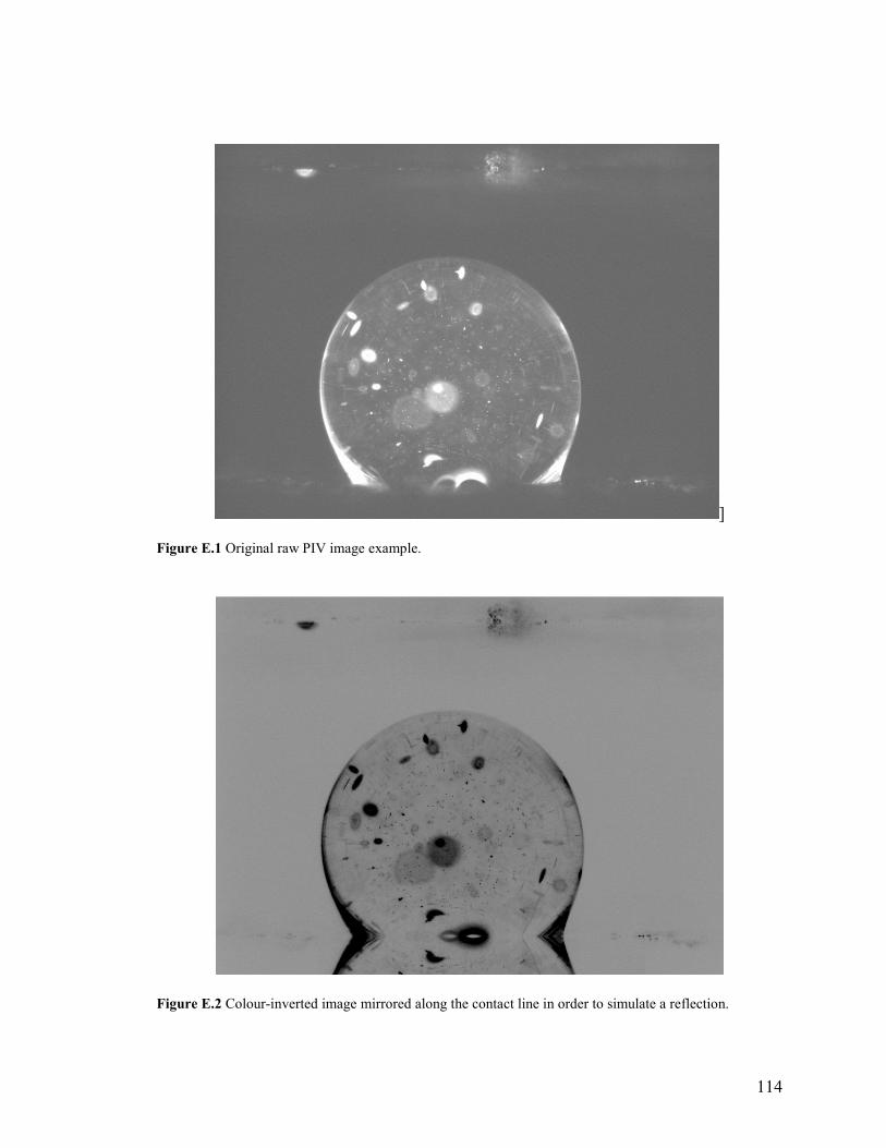
114

]

Figure E.1 Original raw PIV image example.

Figure E.2 Colour-inverted image mirrored along the contact line in order to simulate a reflection.

115

A horizontal line was then drawn across the image such that it intersected both

contact points. The positioning of this line relative to the contact points was performed

by eye to the best of the experimenter’s abilities. In most cases, the contact points were

blurred due to the physical distortion of the droplet shape near the carbon paper, so their

positions had to be approximated. The droplet image was then copied above this line,

flipped vertically, and pasted below the line in order to simulate a perfect reflection of the

droplet. The completed image after these touch ups is shown in Figure E.2.

In some cases, large dark blotches inside the droplet had to be removed as they

would have interfered with the dropsnake plugin’s B-spline algorithms. Also,

occasionally the inflection point at the contact line had to be touched up using Microsoft

Paint in order to eliminate noise or distortions that would have caused an obvious

incorrect reading of the contact angle. These touch ups were performed by eye to the

best of the experimenter’s ability.

The result of the dropsnake plugin on the touched-up image from Figure E.2 is

shown in Figure E.3. Two B-spline curves are shown, one lower resolution blue curve

from the first iteration with less anchor points, and one higher resolution curve from the

second iteration with more nodes. The calculated contact angles are represented with

tangent lines drawn at the contact points, and are printed in the top left corner of the

image.

116

Figure E.3 Colour-inverted image mirrored along the contact line in order to simulate a reflection.

During this experiment, there was often some degree of disagreement in the

calculated contact angles between the results from the first and second iterations, as

demonstrated in Figure E.3. In those cases, the experimenter used his discretion to

decide whether the first result or the second result was a more physically representative

approximation of the contact angle. If it was too difficult to determine this, then the

results from both iterations would simply be averaged.

117

Appendix F Top-View PIV Measurement Example

Although a top-view chip was developed for this experiment, the acquisition of a

set of data using this chip, and the development of modified optical distortion correction

algorithms to correct the images, proved to be beyond the time scope of this Masters

project. A few proof-of-concept vector fields were acquired however, and will be

presented in this appendix.

Figure F.1 shows a photograph of a droplet sitting on the carbon paper surface

from a top view. The focal plane has been aligned with the carbon paper, in order to

make a y-axis zero reference (see Figure 2.16).

Figure F.1 A droplet sitting on the carbon paper surface of the channel in the top view chip. The focal

plane has been aligned with the carbon paper surface as a as a y-axis zero reference point.

118

Figure F.2 A droplet sitting on the carbon paper surface of the channel in the top view chip. The focal

plane has been advanced 0.35 mm in the posititive y-direction to focus on the approximate vertical center

plane of the droplet.

Figure F.2 shows the same droplet, but the focal plane has been advanced 0.35

mm in the positive y-direction in order to perform a measurement in the approximate

vertical center plane of the droplet. 0.35 is approximately half the average height of the

droplets measured in the primary side-view experiments. The droplet is seeded with

fluorescent particles as in the primary experiment.

An air flow of 2.2 m/s was induced in the channel and the same micro-DPIV

measurement process was followed as described in Section 2.3. A raw particle image and

the calculated vector field result, uncorrected for optical distortion, are shown below in

Figures F.3 and F.4 respectfully.

119

Figure F.3 A raw particle image from the droplet in Figures A14 and A15.

Figure F.4 The vector result from 30 pairs of raw images similar to that shown in Figure A18.

120

The top view scenario obviously presents a different set of unique challenges for

PIV image processing than those presented by the side view. For instance, the droplet

profile is almost circular in Figure F.3, and so the three dimensional shape approximation

discussed in Appendix D would have to be modified to account for the change in

perspective.

The vector field results shows an interesting set of nearly symmetrical, counter-

rotating regions in the fluid flow. The counter-rotating regions are intuitive. However,

the air flow is from right to left, but the vectors at the edge of the droplet appear to be

moving against the air flow, which is highly counterintuitive.

This proof-of-concept vector field can only be commented on generally and in a

qualitative sense, since a significant set of data was not obtained, processed, and analyzed

from the top view chip. However, if the focal plane could be moved such that it is in line

with the very peak of the droplet closest to the observer, then it is possible that point-wise

velocity measurements could be made very close to the air-liquid interface that are free of

optical distortion. This is another suggested avenue of pursuit for future work.